Embed Size (px)
Citation preview

Patterns and Variability of Projected Bioclimatic Habitatfor Pinus albicaulis in the Greater Yellowstone AreaTony Chang*, Andrew J. Hansen, Nathan Piekielek
Department of Ecology, Montana State University, Bozeman, Montana, United States of America
Abstract
Projected climate change at a regional level is expected to shift vegetation habitat distributions over the next century. Forthe sub-alpine species whitebark pine (Pinus albicaulis), warming temperatures may indirectly result in loss of suitablebioclimatic habitat, reducing its distribution within its historic range. This research focuses on understanding the patterns ofspatiotemporal variability for future projected P.albicaulis suitable habitat in the Greater Yellowstone Area (GYA) through abioclimatic envelope approach. Since intermodel variability from General Circulation Models (GCMs) lead to differingpredictions regarding the magnitude and direction of modeled suitable habitat area, nine bias-corrected statistically down-scaled GCMs were utilized to understand the uncertainty associated with modeled projections. P.albicaulis was modeledusing a Random Forests algorithm for the 1980–2010 climate period and showed strong presence/absence separations bysummer maximum temperatures and springtime snowpack. Patterns of projected habitat change by the end of the centurysuggested a constant decrease in suitable climate area from the 2010 baseline for both Representative ConcentrationPathways (RCPs) 8.5 and 4.5 climate forcing scenarios. Percent suitable climate area estimates ranged from 2–29% and 0.04–10% by 2099 for RCP 8.5 and 4.5 respectively. Habitat projections between GCMs displayed a decrease of variability over the2010–2099 time period related to consistent warming above the 1910–2010 temperature normal after 2070 for all GCMs. Adecreasing pattern of projected P.albicaulis suitable habitat area change was consistent across GCMs, despite strongdifferences in magnitude. Future ecological research in species distribution modeling should consider a full suite of GCMprojections in the analysis to reduce extreme range contractions/expansions predictions. The results suggest thatrestoration strageties such as planting of seedlings and controlling competing vegetation may be necessary to maintainP.albicaulis in the GYA under the more extreme future climate scenarios.
Citation: Chang T, Hansen AJ, Piekielek N (2014) Patterns and Variability of Projected Bioclimatic Habitat for Pinus albicaulis in the Greater Yellowstone Area. PLoSONE 9(11): e111669. doi:10.1371/journal.pone.0111669
Editor: Ben Bond-Lamberty, DOE Pacific Northwest National Laboratory, United States of America
Received May 30, 2014; Accepted August 20, 2014; Published November 5, 2014
Copyright: � 2014 Chang et al. This is an open-access article distributed under the terms of the Creative Commons Attribution License, which permitsunrestricted use, distribution, and reproduction in any medium, provided the original author and source are credited.
Data Availability: The authors confirm that all data underlying the findings are fully available without restriction. All relevant data are deposited with theKnowledge Network for Biocomplexity: https://knb.ecoinformatics.org/#view/doi:10.5063/F1DZ067F.
Funding: This work was supported by the National Aeronautics and Space Administration Applied Sciences Program (Grant 10-BIOCLIM10-0034); Funder URL:http://www.nasa.gov (AJH TC). It also received support from the National Science Foundation Experimental Program to Stimulate Competitive Research (EPSCoR)Track-I EPS-1101342 (INSTEP 3); Funder URL: http://www.nsf.gov/div/index.jsp?div = EPSC (NBP TC); and the North Central Climate Science Center (G13AC00392-G-8829-1); Funder URL: http://www.doi.gov/csc/northcentral/index.cfm (AJH NBP). The funders had no role in study design, data collection and analysis, decision topublish, or preparation of the manuscript.
Competing Interests: The authors have declared that no competing interests exist.
* Email: [email protected]
Introduction
Over the next century, it is expected that most of North
America will experience climate changes related to increased
concentrations of anthropogenic greenhouse gas emissions and
natural variability [1]. At regional scales these changes are highly
variable and can result in areas of increased mesic, xeric, or even
hydric habitat conditions relative to present day. These shifting
climates in turn also transform the suitable habitat for individual
species that may result in changes in species composition and
dominant vegetation types.
Whitebark pine (Pinus albicaulis) is a native conifer of the
Western U.S. that is considered a keystone species in the sub-
alpine environment. It provides a food source for animals such as
the grizzly bear (Ursus arctos), red squirrel (Tamiasciurushudsonicus), and Clark’s nutcracker (Nucifraga columbiana) [2].
It also serves the ecosystem functions of stabilizing soil, moderating
snow melt and runoff, and facilitating establishment for other
species [2,3]. Whitebark pine has experienced a notable decline in
the past two decades within the U.S. Northern Rockies due to high
rates of infestation from the mountain pine beetle (Dendroctonusponderosae) and infections from white pine blister rust (Cronartiumribicola), resulting in an 80% mortality rate within the adult
population [4–7]. Given the potential loss of important ecosystem
functions that whitebark pine contribute to the landscape under
this mortality event, there is an emphasis to understand the climate
characteristics of its habitat to identify the restoration strategies
and locations that may aid the persistence of the species under
future climates.
One method of understanding species response to climate
change is through bioclimate niche modeling, which has become a
common practice for assessing potential vegetation shifts under
new environmental conditions [8–13]. Ecological niche theory
proposes there exists some range of bioclimatic conditions within
which a species can persist [14]. In bioclimatic niche modeling, the
realized niche is modeled by empirical relationships between the
presence or absence of a species and the associated abiotic, and
PLOS ONE | www.plosone.org 1 November 2014 | Volume 9 | Issue 11 | e111669

sometimes biotic, variables that describe the niche space.
Bioclimatic models assume that species are in equilibrium with
their environment and that the current abiotic relationships reflect
a species environmental preferences which may be retained into
the future [15,16]. At macro scales, bioclimatic approaches have
demonstrated success at predicting current distributions of species
[17,18]. Most bioclimatic models do not explicitly consider the
many additional ecological factors that ultimately influence a
species distribution such as dispersal, disturbance, or biotic
interaction. Thus the approach does not predict where a species
will actually occur in the future, but rather it predicts locations
where climatic conditions will be suitable for the species.
Bioclimatic niche methodology has demonstrated utility in
modeling historic ranges of species for conservation and manage-
ment applications. By modeling the present day suitable habitat
and then projecting those habitats into the future, bioclimatic
Figure 1. Historic and projected climates variables for the GYA from 1895–2099 under RCP 4.5 and 8.5 scenarios. Light shaded orangeand red lines represent individual GCMs for RCP 4.5 and 8.5 respectively. Bold lines represent GCM ensemble average. (a) Mean annual temperature(b) Mean annual precipitation.doi:10.1371/journal.pone.0111669.g001
Figure 2. The Greater Yellowstone Area, representing an area of 150,700 km2 with an elevational gradient from 522–4,206 m.doi:10.1371/journal.pone.0111669.g002
Projected Bioclimate Habitat for Pinus albicaulis in the GYA
PLOS ONE | www.plosone.org 2 November 2014 | Volume 9 | Issue 11 | e111669
niche models can serve as the first step filter for conservation
action plans, such as mapping suitable species reintroduction sites
or habitat reserve selection [19–21]. For P.albicaulis, McLane and
Aitken [22] utilized bioclimate niche models to successfully
implement experimental assisted migration on persisting climate
habitat in British Columbia. Additionally, models of Pinus flexis, a
closely related species of five needle pine, have been used to
evaluate management options in Rocky Mountain National Park
[23]. Given these examples, an effort to model and projected
suitable climate habitat for P.albicaulis within a regional domain
can provide valuable insight to land resource managers.
In this study, we present a bioclimatic habitat model for
P.albicaulis within the Greater Yellowstone Area (GYA). Al-
though P. albicaulis has a range-wide distribution that is split into
two broad sections, one along Western North America: the British
Columbia Coast Range, the Cascade Range, and the Sierra
Nevada; and the other section in the Intermountain West that
covers the Rocky Mountains from Wyoming to Alberta [2,24]; the
GYA was selected as the primary geographic modeling domain for
three reasons: 1) evidence that the P. albicaulis sub-population in
the GYA is genetically distinct from other regional populations
with different climate tolerances [25]; 2) the high regional
investment in P. albicaulis conservation in the area [6]; 3) the
high density of climate stations within the region. Climate within
the GYA is highly heterogenous due to complex topography, and
sharp elevational gradients. Current knowledge of the region
expects climate to shift towards increased mean annual temper-
atures and earlier spring snowmelt [26,27]. This shift is expected
to have an impact on the total suitable habitat area for P.albicaulis. Modeling at a regional scale can provide a finer
resolution spatially explicit description of the bioclimatic envelope
of P. albicaulis in the GYA.
Here we also present an opportunity to investigate the effect of
future climate variability on projected species distributions. In
2013, the World Climate Research Programme Coupled Model
released the new generation General Circulation Model (GCM)
projections through the Coupled Model Intercomparison Project
Phase 5 (CMIP5) [28]. These new GCM projections also include
four possible climate futures are modeled with each GCM under
the Representative Concentration Pathways (RCP) of greenhouse
gas/aerosol. These RCP scenarios designate four different levels of
radiative forcing (2.6, 4.5, 6.0 and 8.5 W/m2) that may occur by
the year 2099 [29]. In practice, research of future species suitable
climate generally use a small suite of GCM/RCP combinations to
project future climate [8,11,30]. However, internal variability in
these GCMs that arise from modeled coupled interactions among
the atmosphere, oceans, land, and cryosphere can result in
atmospheric circulation fluctuations that are characteristic of a
stochastic process [31]. Such intrinsic atmospheric circulation
variations from model structure induce regional changes in air
temperature and precipitation on the multi-decadal time scale
[31]. For the GYA specifically, this GCM variability has be
observed with mean annual temperatures projected to increase by
2{9uC and mean annual precipitation to change by 250 to +225 mm (Fig. 1). This suggests that magnitude and direction of
projected species distributions at a regional scale can vary
depending on the GCM selected and the modeled species
response to more xeric or mesic future climate conditions [32].
To summarize, this study presents a bioclimate niche model for
P. albicaulis based on historic climate observations and field
sampling of P. albicaulis presence and absence. Using this
modeled bioclimate envelope, projections of future total climate
suitable habitat area under nine GCMs and two RCP scenarios
will be measured. Since different GCMs may project a diverging
spectrum of climates, it is expected that measures of total suitable
habitat will reduce with varying degrees of area loss. It is also
expect that number and size of continous patches of P. albicaulishabitat will reduce due to the limited available number of sub-
alpine areas distributed within the landscape. This research
provides an analysis of the variability of biotic response under a
large suite of GCMs to provide managers/researchers with a
measure of the uncertainty associated with future species
distribution models. Furthermore, this analysis explicitly describes
the spatial patterns of bioclimatic niches for P. albicaulis to gain a
better understanding of topographic characteristics, such as
elevation, on suitable habitat. Changes in these spatial patterns
are examined through quantifying landscape patch dynamic that
may result from GCM projections to understand the species trends
for persistence on the landscape.
Methods
Study areaThe GYA, which includes Yellowstone National Park, Grand
Teton National Park, and a number of state and federally
managed forests, is a mid- to high-latitude region in the Northern
Rocky Mountains of western North America. Conifers are
dominant in the range, with forest types composed of Pinuscontorta, Abies lasiocarpa, Pseudotsuga menziesii, Pinus albicaulis,Juniperus scopulorum, Pinus flexis and Picea engelmannii,
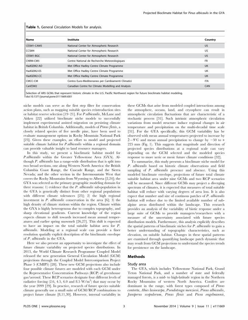
Table 1. General Circulation Models for analysis.
Name Institute Country
CESM1-CAM5 National Center for Atmospheric Research US
CCSM4 National Center for Atmospheric Research US
CESM1-BGC National Center for Atmospheric Research US
CNRM-CM5 Centre National de Recherche Meteorologiques FR
HadGEM2-AO Met Office Hadley Centre Climate Programme UK
HadGEM2-ES Met Office Hadley Centre Climate Programme UK
HadGEM2-CC Met Office Hadley Centre Climate Programme UK
CMCC-CM Centro Euro-Mediterraneo per Cambiamenti Climatici ITA
CanESM2 Canadian Centre for Climate Modelling and Analysis CAN
Selection of AR5 GCMs that represent historic climate in the U.S. Pacific Northwest region for future bioclimate habitat modeling.doi:10.1371/journal.pone.0111669.t001
Projected Bioclimate Habitat for Pinus albicaulis in the GYA
PLOS ONE | www.plosone.org 3 November 2014 | Volume 9 | Issue 11 | e111669

although the deciduous hardwood Populus tremuloides, is also
wide spread. Plateaus and lowlands are dominated by species of
Artemisia tridentata and open grasslands of mixed composition.
The GYA study area encompasses 150,700 km2 with an
elevational gradient from 522–4,206 m that represents 14
surrounding mountain ranges (Fig. 2).
DataBiological data. Field observations of P. albicaulis adult
presences and absences were compiled from three data sources.
First, 2,545 observations from the Forest Inventory and Analysis
(FIA) program were assembled. FIA plots are located on a regular
gridded sampling design with one plot at approximately every
2,500 forested hectares, with swapped and fuzzed exact plot
locations within 1.6 km to protect privacy [33]. Gibson et al. [34]
found that model accuracy to not be dramatically affected by data
fuzzing, but to provide the most spatial accuracy, this study culled
FIA field points where measured elevation were w300 m different
from a 30 m USGS DEM [35]. To capitalize on additional field
observations of P. albicaulis within the study area, and because
false absences are one of the most problematic data issues in
constructing bioclimatic niche models [36]; supplementary points
were drawn from the Whitebark/Limber Pine Information System
(WLIS) [37], and long-term monitoring plots established by the
Figure 3. Selected predictor variables based on Principal Component Analysis and a maximum correlation filter of ƒ0.75. Scatterplots represent one-to-one covariate plots where red points represent P. albicaulis presence, and blue points represent absence from field data. Far-left columns display logistic-regression of covariates from Generalized Additive Modeling using the Software for Assisted Habitat Modeling (SAHM[59]).doi:10.1371/journal.pone.0111669.g003
Projected Bioclimate Habitat for Pinus albicaulis in the GYA
PLOS ONE | www.plosone.org 4 November 2014 | Volume 9 | Issue 11 | e111669

National Park Service Greater Yellowstone Inventory and
Monitoring Network (GYRN) [38]. The presences in these two
additional datasets were collocated within predictor pixels of FIA
absence to correct for false absences. In doing so, only one P.albicaulis presence or absence record was associated per predictor
pixel, thereby avoiding issues associated with sampling bias that
are common when building bioclimate niche models with data
from targeted surveys [39]. This compilation of data represents an
effort for ‘‘completeness’’ as described by Kadmon et al. [40] and
Franklin [36], to capture all climate conditions where a species
does exist. New data sources added 119 P. albicaulis presences
that would have been missed by using FIA data alone, for a total of
938 presences and 1,633 absences.
‘‘Adult’’ class P. albicaulis were selected for modeling based on
a recorded diameter at breast height (DBH) w20 cm. P. albicauliswithin the Central Montana are reported to reach 100 years of age
at approximately 8–12 m in height with DBHs between 15–20 cm
[41]. Given previous silvicultural studies, it was assumed that
20 cm DBH P. albicaulis represent adult class individuals for the
GYA, with potential to reproduce [24]. Furthermore, this study
focused on adult size class due to difficulties distinguishing younger
age class P. albicilus from P. flexis.Historic climate data. Climate inputs for modeling were
acquired from the 30-arc-second (*800 m) monthly Parameter-
elevation Regressions on Independent Slopes Model (PRISM), a
derived product that interpolates local station measurements
across a continuous grid [42]. PRISM data includes monthly
average minimum temperatures (Tmin), maximum temperature
(Tmax), mean temperature (Tmean), and mean precipitation (Ppt).
All monthly data were averaged for the temporal extent of 1950–
1980 for bioclimatic niche model fitting. The 1950–1980 temporal
extent was selected for modeling since: 1) a sufficient density of
weather stations were operating by 1950 to provide a reasonable
network; 2) evidence of anthropogenic warming that begins in the
Table 2. Bioclimatic predictor variable list.
Code Predictor Variable
tmin1 Minimum Temperature January
vpd3 Vapor Pressure Deficit March
ppt4 Precipitation April
pack4 Snow Water Equivalent April
tmax7 Maximum Temperature July
aet7 Actual Evapotranspiration July
pet8 Potential Evapotranspiration August
ppt9 Precipitation September
Final predictor variable set for Random Forest modeling. All variables were calculated as a 30-year climate mean from 1950–1980.doi:10.1371/journal.pone.0111669.t002
Figure 4. Area under curve for the receiver operating characteristic plot suggests adequate performance from the Random Forestmodeling.doi:10.1371/journal.pone.0111669.g004
Projected Bioclimate Habitat for Pinus albicaulis in the GYA
PLOS ONE | www.plosone.org 5 November 2014 | Volume 9 | Issue 11 | e111669

late 1980s; 3) trees old enough to bear seeds today likely
established under a similar climates to the 1950–1980 period.
Water balance. A Thornthwaite-based dynamic water bal-
ance model was used to estimate a number of variables that
include actual evapotranspiration (AET) and potential evapo-
transpiration (PET) [43–45]. The model required only monthly
mean temperatures, dew point temperatures, and precipitation
(see Text S1). Water was stored as soil moisture or in surface
snowpack, with the excess taking the form of evaporated vapor or
loss through seepage/runoff. In addition to the climatic variables,
latitude and physical characteristics of the soil were required to
define water holding capacity. Soil attributes assigned by the Soil
Survey Geographic (STATSGO) datasets were allocated from the
Natural Resource Conservation Service at a 30-arc-second
resolution to determine soil water holding capacity and estimates
for soil depth [46]. All water balance variables, which include
PET, AET, soil moisture, vapor pressure deficit (vpd), and snow
water equivalent (pack), were averaged by month over 1950–1980
to match with historic climate data for bioclimate model fitting.
GCM data. The general circulation model (GCM) experi-
ments conducted under CMIP5 for the Intergovernmental Panel
on Climate Change Fifth Assessment Report provided future
projected climate data sets for assessing the effects of global climate
change. Using a Bias-Correction Spatial Disaggregation (BCSD)
approach, an archive of statistically down-scaled CMIP5 climate
projections for the conterminous United States at 30-arc-second
spatial resolution was assembled by the NASA Center for Climate
Simulation NEX-DCP30 [47]. For this analysis, a subset of the
Figure 5. Threshold for probability of presence of 0.421 determined at the intersection of true positive rate (TPR) and true negativerate (TNR). Equivalent TPR and TNR, displayed a compromise between the maximum true skill statistic (TSS : 0:345) and maximum Kappa statistic(k : 0:538).doi:10.1371/journal.pone.0111669.g005
Table 3. Confusion matrix from out-of-bag analysis.
Validation data set
Presence Absence
Model Presence 763 (81.9%) 169 (13.1%)
Absence 176 (10.9%) 1437 (89.1%)
Random Forest tree estimators displays higher OOB specificity than sensitivity. Area Under Curve (AUC) value of 0.94 suggests model has high predictive capacity forprojecting future suitable bioclimate habitat.doi:10.1371/journal.pone.0111669.t003
Projected Bioclimate Habitat for Pinus albicaulis in the GYA
PLOS ONE | www.plosone.org 6 November 2014 | Volume 9 | Issue 11 | e111669
total GCM models available from NASA were selected that best
represent the Northwestern US. Rupp et al. [48] recently
presented an analysis of GCM performance versus the observed
historic climate in the U.S. Pacific Northwest under 18 specified
climate metrics. In their analysis, Rupp et al. ranked GCMs for
accuracy using an empirical orthogonal function (EOF) analysis of
the total normalized error compared to reference data. This
analysis selected models with a normalized error score v0:5 as a
threshold to cull the full suite of GCMs to the top nine models.
These GCMs were used to project modeled P. albicaulis
distributions into the future (Table 1). Two RCP scenarios were
selected to understand effects of differing carbon futures under
climate change from 2010 to 2099. RCP 4.5 was the first,
representing increased radiative forcing until stabilization of
greenhouse emissions between 2040–2050 and total radiative
forcing of 4.5 W/m2 by 2099. RCP 8.5 was the second,
representing the ‘‘business as usual’’ scenario, with uncontrolled
radiative forcing increasing with stabilization of 8.5 W/m2 by
2099 [49,50].
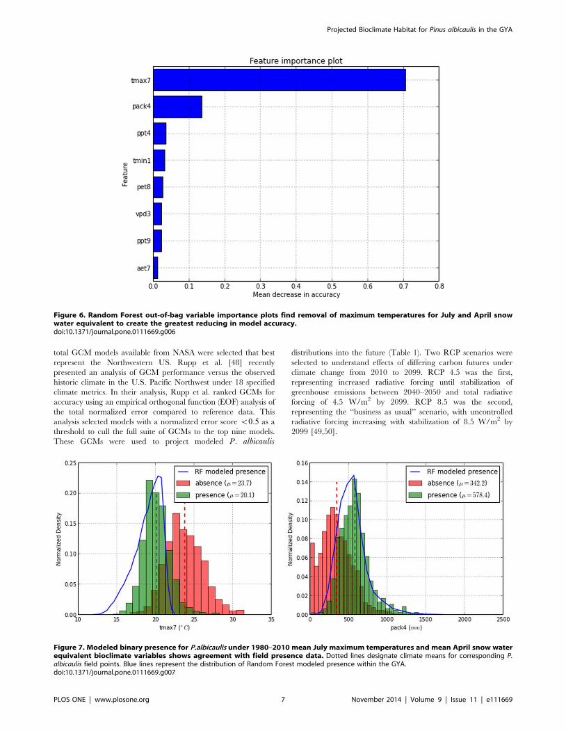
Figure 6. Random Forest out-of-bag variable importance plots find removal of maximum temperatures for July and April snowwater equivalent to create the greatest reducing in model accuracy.doi:10.1371/journal.pone.0111669.g006
Figure 7. Modeled binary presence for P.albicaulis under 1980–2010 mean July maximum temperatures and mean April snow waterequivalent bioclimate variables shows agreement with field presence data. Dotted lines designate climate means for corresponding P.albicaulis field points. Blue lines represent the distribution of Random Forest modeled presence within the GYA.doi:10.1371/journal.pone.0111669.g007
Projected Bioclimate Habitat for Pinus albicaulis in the GYA
PLOS ONE | www.plosone.org 7 November 2014 | Volume 9 | Issue 11 | e111669
Modeling methodsA random forest (RF) [51] algorithm was used to create a
bioclimate niche model of P. albicaulis in the GYA. Random
forest is an ensemble learning technique that generates indepen-
dent random classification trees using a subset of the total
predictor variables and classifies a bootstrap random subsample of
the data. These trees are aggregated and a majority vote over all
trees in the random forest defines the resulting response class. This
method of random trees with subsampling ensures a robust
ensemble classification reducing overfitting and collinearity issues,
especially with a large number of trees [9,51–53]. The python
programming language (Python 3.3) and the Scikit-Learn library
was used to fit the random forest model and predict current
habitat niche, with parameters for number of trees
(nestimators~1000), number of variables (maxfeatures~4), and node
size (minsamplesleaf ~20) [54].
First pass filtering of environmental covariates was performed
using Principal Component Analysis (PCA) to generate proxy sets
[55–57]. After initial list was constructed, an additional filter was
imposed on the variables with a 0.75 maximum correlation
threshold to avoid collinearity issues (Fig. 3) [55]. Physiologically
relevant variables to P. albicaulis presence were given precidence
in final culling in cases of correlation above the specified
maximum threshold. The final variable list selected were tmin1,
vpd3, ppt4, pack4, tmax7, aet7, pet8, ppt9 (Table 2). The
Software for Assisted Habitat Modeling (SAHM) was used to
visualize correlations with the pairs function embeded in the
VisTrails scientific workflow management system [58,59].
Model evaluation was performed under a variety of methods.
An out-of-bag (OOB) error estimate was calculated by comparing
the modeled probability of presence using approximately two-
thirds of the field data, while withholding a subset of the
remainder. Accuracy was evaluated by calculating: 1) the
sensitivity, representing the true positive rate (TPR), 2) the
specificity, representing the true negative rate (TNR), 3) the
receiver operator characteristic curve (AUC). Importance of a
specific predictor variable was calculated by examination of the
increase in prediction error within the OOB sample when the
predictor variable was permuted while others were held constant
[54,60]. The rate of prediction error with permutation of a
specified variable can be interpreted as the level of dependence of
presence or absence response to that variable [61].
Projections for P. albicaulis were computed using 30 year
moving climate averages for the period from 2010–2099 for both
RCP 4.5 and 8.5 climate scenarios. Changes of suitable habitat
area were determined using a binary classification of expected
presence and absence. Binary class assignment was made under a
probability of presence threshold where the ratio of sensitivity and
specificity equalled 1. This method ensured an equal ability of the
model to detect presence and absence. The Kappa and True Skill
Statistic (TSS) were also calculated to observe how sensitivity and
specificity responded under differing probability thresholds [62].
Survey plots predicted as suitable under climatic conditions in
2010 served as a reference for projections. The presence
classifications were evaluated as the amount of suitable habitat
changed over time, confined within specified elevational limits. To
account for the need for a minimum patch size, total number of
patches and median sizes using the an eight-neighbor rule (see
Text S1) for patch identification were tracked over time [63].
Results
Model evaluationThe random forest model displayed an out-of-bag (OOB) error
rate of 16.1% with greater errors of commission (13.1%) than
omission (10.9%) (Table 3). The AUC was 0.94, displaying high
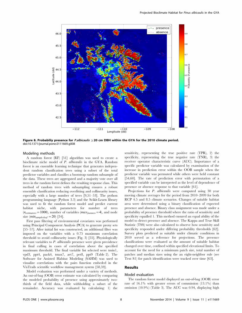
Figure 8. Probabiliy presence for P.albicaulis §20 cm DBH within the GYA for the 2010 climate period.doi:10.1371/journal.pone.0111669.g008
Projected Bioclimate Habitat for Pinus albicaulis in the GYA
PLOS ONE | www.plosone.org 8 November 2014 | Volume 9 | Issue 11 | e111669

specificity and sensitivity (Fig. 4). Threshold probability of
presence for a binary classification was selected at 0.421 (i.e
where sensitivity = specificity). A probability threshold where
TPR and TNR were equal was compared to the maximum Kappa
statistic (0.538) and the maximum True Skill Statistic (TSS) (0.345)
and found to be a compromise between the diagnostics (Fig. 5).
Estimates of variable importance plots revealed that permuta-
tion of maximum temperatures of summer months from all
random trees resulted in a large drop in mean accuracy for
distinguishing presence and absence of P. albicaulis (0:706decrease in mean accuracy). This was followed by spring time
snowpack (0:137 decrease in mean accuracy) (Fig. 6). Histogram
plots of July maximum temperatures and April snowpack provided
evidence of discrimination for presence and absence that are
consistent with the modeled probability of presence for the year of
calibration (Fig. 7).
Spatially explicit probability plots for the 2010 climate displayed
highest probability of presence values within the §2500 m
mountain ranges of the GYA in agreement with studies employing
aerial imagery and remote sensing [4,5] (Fig. 8). Assuming that the
modeled suitable bioclimate for P. albicaulis remains similar in the
next century, the model demonstrated capacity to predict probable
future P. albicaulis suitable habitat under projected climate
conditions.
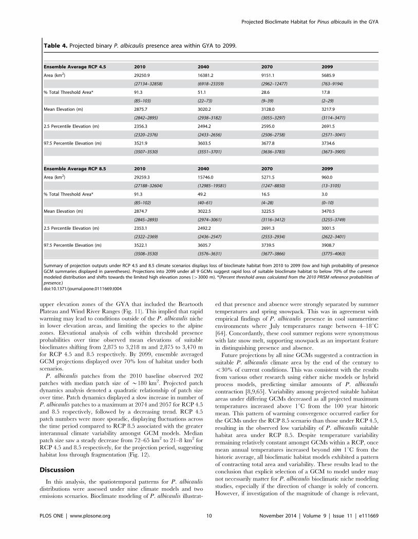
Model projectionsUnder both RCP 4.5 and 8.5, there was a predicted steady
reduction of suitable bioclimate habitat for P. albicaulis over the
course of this century, with RCP 8.5 displaying steeper declines
than RCP 4.5 (Fig. 9). Under the RCP 4.5 and 8.5 scenarios,
suitable habitat shifts from 100–85% to 2–29% by 2099, and 100–
85% to 0.04–10% by 2099 respectively (Table 4).
CNRM-CM5, CMCC-CM, and CESM1-BGC projections
showed the highest probabilities for suitable habitat area at the
end of the century, while HadGEM2-AO, HadGEM2-ES, and
HadGEM2-CC indicated the lowest probabilities. The standard
deviations per year for both RCPs progressively decreased over
time (Fig. 10). Among climate scenarios, standard deviations for
both RCPs display low variability for the first five projection years
and a rapid increase of variability peaking at 2043. For RCP 4.5,
high variability existed primarily due to differing climate
projections by models HadGEM2-AO and HadGEM2-CC,
resulting in uncertainties in probabilities of presence fluctuating
between 8 and 15% until 2068, after which variability was
between 6–8%. Under RCP 8.5, standard deviations between
GCMs were consistently lower than RCP 4.5. Regardless of the
GCM, by 2079 the areas of suitable habitat converged to similar
values.
Spatially explicit mapping of probability surfaces presented
similar contractions of P. albicaulis habitat suitability toward the
Figure 9. Bioclimate projections for P.albicaulis for 2010 to 2099 under 30-year moving averaged climates.doi:10.1371/journal.pone.0111669.g009
Projected Bioclimate Habitat for Pinus albicaulis in the GYA
PLOS ONE | www.plosone.org 9 November 2014 | Volume 9 | Issue 11 | e111669
upper elevation zones of the GYA that included the Beartooth
Plateau and Wind River Ranges (Fig. 11). This implied that rapid
warming may lead to conditions outside of the P. albicaulis niche
in lower elevation areas, and limiting the species to the alpine
zones. Elevational analysis of cells within threshold presence
probabilities over time observed mean elevations of suitable
bioclimates shifting from 2,875 to 3,218 m and 2,875 to 3,470 m
for RCP 4.5 and 8.5 respectively. By 2099, ensemble averaged
GCM projections displayed over 70% loss of habitat under both
scenarios.
P. albicaulis patches from the 2010 baseline observed 202
patches with median patch size of *180 km2. Projected patch
dynamics analysis denoted a quadratic relationship of patch size
over time. Patch dynamics displayed a slow increase in number of
P. albicaulis patches to a maximum at 2074 and 2057 for RCP 4.5
and 8.5 respectively, followed by a decreasing trend. RCP 4.5
patch numbers were more sporadic, displaying fluctuations across
the time period compared to RCP 8.5 associated with the greater
interannual climate variability amongst GCM models. Median
patch size saw a steady decrease from 72–65 km2 to 21–8 km2 for
RCP 4.5 and 8.5 respectively, for the projection period, suggesting
habitat loss through fragmentation (Fig. 12).
Discussion
In this analysis, the spatiotemporal patterns for P. albicaulisdistributions were assessed under nine climate models and two
emissions scenarios. Bioclimate modeling of P. albicaulis illustrat-
ed that presence and absence were strongly separated by summer
temperatures and spring snowpack. This was in agreement with
empirical findings of P. albicaulis presence in cool summertime
environments where July temperatures range between 4–18uC[64]. Concordantly, these cool summer regions were synonymous
with late snow melt, supporting snowpack as an important feature
in distinguishing presence and absence.
Future projections by all nine GCMs suggested a contraction in
suitable P. albicaulis climate area by the end of the century to
v30% of current conditions. This was consistent with the results
from various other research using either niche models or hybrid
process models, predicting similar amounts of P. albicauliscontraction [8,9,65]. Variability among projected suitable habitat
areas under differing GCMs decreased as all projected maximum
temperatures increased above 1uC from the 100 year historic
mean. This pattern of warming convergence occurred earlier for
the GCMs under the RCP 8.5 scenario than those under RCP 4.5,
resulting in the observed low variability of P. albicaulis suitable
habitat area under RCP 8.5. Despite temperature variability
remaining relatively constant amongst GCMs within a RCP, once
mean annual temperatures increased beyond sim 1uC from the
historic average, all bioclimatic habitat models exhibited a pattern
of contracting total area and variability. These results lead to the
conclusion that explicit selection of a GCM to model under may
not necessarily matter for P. albicaulis bioclimatic niche modeling
studies, especially if the direction of change is solely of concern.
However, if investigation of the magnitude of change is relevant,
Table 4. Projected binary P. albicaulis presence area within GYA to 2099.
Ensemble Average RCP 4.5 2010 2040 2070 2099
Area (km2) 29250.9 16381.2 9151.1 5685.9
(27134–32858) (6918–23359) (2962–12477) (763–9194)
% Total Threshold Area* 91.3 51.1 28.6 17.8
(85–103) (22–73) (9–39) (2–29)
Mean Elevation (m) 2875.7 3020.2 3128.0 3217.9
(2842–2895) (2938–3182) (3055–3297) (3114–3471)
2.5 Percentile Elevation (m) 2356.3 2494.2 2595.0 2691.5
(2320–2376) (2433–2656) (2506–2758) (2571–3041)
97.5 Percentile Elevation (m) 3521.9 3603.5 3677.8 3734.6
(3507–3530) (3551–3701) (3636–3783) (3673–3905)
Ensemble Average RCP 8.5 2010 2040 2070 2099
Area (km2) 29259.3 15746.0 5271.5 960.0
(27188–32604) (12985–19581) (1247–8850) (13–3105)
% Total Threshold Area* 91.3 49.2 16.5 3.0
(85–102) (40–61) (4–28) (0–10)
Mean Elevation (m) 2874.7 3022.5 3225.5 3470.5
(2845–2893) (2974–3061) (3116–3412) (3255–3749)
2.5 Percentile Elevation (m) 2353.1 2492.2 2691.3 3001.5
(2322–2369) (2436–2547) (2553–2934) (2622–3401)
97.5 Percentile Elevation (m) 3522.1 3605.7 3739.5 3908.7
(3508–3530) (3576–3631) (3677–3866) (3775–4063)
Summary of projection outputs under RCP 4.5 and 8.5 climate scenarios displays loss of bioclimate habitat from 2010 to 2099 (low and high probability of presenceGCM summaries displayed in parentheses). Projections into 2099 under all 9 GCMs suggest rapid loss of suitable bioclimate habitat to below 70% of the currentmodeled distribution and shifts towards the limited high elevation zones (w3000 m). *(Percent threshold areas calculated from the 2010 PRISM reference probabilities ofpresence.)doi:10.1371/journal.pone.0111669.t004
Projected Bioclimate Habitat for Pinus albicaulis in the GYA
PLOS ONE | www.plosone.org 10 November 2014 | Volume 9 | Issue 11 | e111669
Figure 10. Evaluation of the standard deviation s for percent suitable habitat area by RCP scenario.doi:10.1371/journal.pone.0111669.g010
Figure 11. Spatially explicit probabilty surfaces for 2040 to 2099 suggest contraction of suitable bioclimatic habiatat for P.albicaulisinto the §2500 m elevation zones.doi:10.1371/journal.pone.0111669.g011
Projected Bioclimate Habitat for Pinus albicaulis in the GYA
PLOS ONE | www.plosone.org 11 November 2014 | Volume 9 | Issue 11 | e111669
then GCM selection may directly influence the projected total
suitable habitat area. This can be observed with RCP 4.5 habitat
projection models differing by as much as 27% total suitable
habitat area by the year 2099. Therefore arbitrary selection of a
GCM for future projection modeling is likely inappropriate since it
could lead to overly optimistic/pessimistic results for the species of
concern.
Temporal patch dynamic analysis present an increase in
fragmentation of the larger P. albicaulis suitable habitats over
the next five decades, suggested through an increase in the total
number of continuous patches but decreases in median size. This
was followed by a contraction of small patches until they were
almost absent from the system. Remaining habitat patches were
smaller and less prevalent on the landscape by the end of the
century. Reduced habitat patch size and density may reduce the
likelihood for N. columbiana to disperse successful germinating
seed caches, due to the limited size and area of suitable patch
space. If changing climate habitats result in mortality within adult
patches, genetic diversity may be lost resulting in a population
bottleneck, thus reducing the robustness of the species to adapt to
future disturbances. Experimental trials of P. albicaulis survival
and fecundity under warmer and drier conditions outside the
currently known range would provide greater confidence of the
species ability to persist under future change. Limited analysis on
seedling environmental conditions would also elucidate spatially
explicit dispersal ranges and greater understanding of probable
ranges for future establishment and survivorship.
Projected distributions of persistent P. albicaulis patches
displayed a strong trend towards contraction into high elevation
zones. Physiologically, there does not appear to be any upper
elevation limit for P. albicaulis in the GYA. P. albicaulis in the
region has been reported to survive in absolute temperatures as
low as 236uC [64]. Lab experiments performed on Pinus cembra,
a related five-needle pine residing in similar climates, were able to
endure cold temperature extremes as low at 270uC without
cellular tissue damage [66]. Considering the current absolute
minimum temperatures the species resides in and cold tolerance of
its relatives suggests that P. albicaulis treeline in the GYA are not
limited by lower temperatures. Controlled laboratory experimen-
tation on P. albicaulis tolerances to temperatures would greatly
improve this physiological understanding of cold tolerance.
Elevational habitat constriction do not imply that P. albicauliswill be completely gone from the region, but merely the loss of
suitable climate habitat. Currently pre-established adult age class
individuals will likely persist, since projected conditions of
increased temperatures and CO2 concentrations physiologically
indicate increased growth rates of P. albicaulis [67]. Furthermore,
micro-refugia sites may exist in the GYA that support P. albicaulissurvival into the future, but were failed to have been modeled due
to the coarseness of 30-arc-second climate data resolution. Since
this bioclimatic envelope modeling approach was parameterized
by the realized niche from in-situ data, it was difficult to determine
if lower elevation limits are driven by warmer climate conditions
or competition for light, water, or nutrients [15,17]. For example,
lower treeline limits for P. albicaulis maybe driven primarily by
competitive exclusion from late seral species A.lasiocarpa,P.contorta, and P.engelmannii. This follows from paleoecological
pollen records of competitor migration during the Early Holocene
(9000–5000 yr B.P), when climate conditions were warmer and
drier. Longer growing seasons allowing competitors to invade
likely drove P. albicaulis communities +500 m in elevation [68–
70]. If future climate conditions become analogous to this Early
Figure 12. Patch dynamics of modeled P.albicaulis. Time series of P.albicaulis patch projections for number of patches and median patch size to2099.doi:10.1371/journal.pone.0111669.g012
Projected Bioclimate Habitat for Pinus albicaulis in the GYA
PLOS ONE | www.plosone.org 12 November 2014 | Volume 9 | Issue 11 | e111669
Holocene period, invasion of competitor species will likely contract
P. albicaulis habitat to the limited high elevation zones of the
GYA, specifically the Beartooth Plateau region and Wind River
range [71].
Conclusion
This analysis examined the future of P. albicaulis suitable
climate in the GYA and explicitly addressed the question of
distribution variability under 9 representative GCMs and 2
emission scenarios. Increases in temperature within the GYA will
likely result in a high level of contraction of suitable climate habitat
for P. albicaulis over the next century. This contraction was
consistent for all GCM projections, with approximately 20%
uncertainty in total probable area. This analysis recommends that
care be taken for species distribution modeling in future studies
during the selection of GCMs due to their relevance for
magnitudes of change. GCM ensemble averaging may be a
solution to this issue, however it should be noted that averaging
should take place after an individual GCM is projected in order to
maintain interannual variability.
Although other studies have examined P. albicaulis species
distribution models [8,65,72], this study is a step forward through
its focus on relevant regional scale design, expansive local datasets,
inclusion of high resolution climate and dynamic water balance
variables, and selective projection under the latest AR5 GCMs. It
is reiterated that the bioclimate niche model approach has high
utility for understanding habitat conditions through correlative
relationships with environmental variables, however, it may fail to
explicitly model competitive exclusion, disturbance, phenotypic
plasticity, and other complex interactions that are vital in
determining a species’ actual presence as it experiences changes
in climate [15,17,73,74]. These unmodeled factors create uncer-
tainties suggesting that this modeling effort does not identify the
full potential climatic range of P. albicaulis in the future.
Uncertainties also exist regarding new suitable climates that may
occur outside the current species range. Despite most rangewide
studies confirming our results of total suitable habitat area
reduction, there is potential for previously unsuitable habitat to
become available under future climate change in the Northern
regions [8,22,65]. Caution is therefore advised to individuals
interpreting these findings. Changing climate will inevitably result
in impacts on biomes and community structures. As such,
mitigation and adaptation for potential futures are vital to
conservation of climate sensitive species [75]. Future research
that combines bioclimatic niche modeling with a mechanistic
based disturbance, dispersal, and competition model will likely
provide greater insight to the potential range of P. albicaulis in a
climate changing world [76,77]. It would furthermore provide
insight towards informing management options for restoration that
may include controlled fire, selected thinning of competitor
species, or assisted migration.
Supporting Information
Text S1 Description of water balance model and 8-neighbor rule
(PDF)
Acknowledgments
We are indebted for the insightful reviews from Richard Waring, William
Monahan, and Tom Olliff. Many thanks to Marian and Colin Talbert, and
Mark Greenwood for the software and statistical consultation.
Author Contributions
Conceived and designed the experiments: TC AJH NBP. Performed the
experiments: TC NBP. Analyzed the data: TC. Contributed reagents/
materials/analysis tools: TC AJH NBP. Wrote the paper: TC AJH NBP.
References
1. Intergovernmental Panel on Climate Change (2007) Fourth Assessment Report:
Climate Change 2007: The AR4 Synthesis Report. Geneva: IPCC.
2. Tomback DF, Arno SF, Keane RE (2001) Whitebark pine communities: ecology
and restoration. Island Press.
3. Callaway RM (1998) Competition and facilitation on elevation gradients in
subalpine forests of the Northern Rocky Mountains, USA. Oikos 82: pp. 561–
573.
4. Macfarlane WW, Logan JA, Kern W (2012) An innovative aerial assessment of
greater yellowstone ecosystem mountain pine beetle-caused whitebark pine
mortality. Ecological Applications.
5. Jewett JT, Lawrence RL, Marshall LA, Gessler PE, Powell SL, et al. (2011)
Spatiotemporal relationships between climate and whitebark pine mortality in
the greater yellowstone ecosystem. Forest Science 57: 320–335.
6. Logan JA, Macfarlane WW, Willcox L (2010) Whitebark pine vulnerability to
climate-driven mountain pine beetle disturbance in the greater yellowstone
ecosystem. Ecological Applications 20: 895–902.
7. Logan JA, Bentz BJ (1999) Model analysis of mountain pine beetle (coleoptera:
Scolytidae) seasonality. Environmental Entomology 28: 924–934.
8. Rehfeldt GE, Crookston NL, Saenz-Romero C, Campbell EM (2012) North
American vegetation model for land-use planning in a changing climate: a
solution to large classification problems. Ecological Applications 22: 119–141.
9. Rehfeldt GE, Crookston NL, Warwell MV, Evans JS (2006) Empirical analyses
of plant-climate relationships for the western United States. International
Journal of Plant Sciences 167: 1123–1150.
10. Thuiller W (2004) Patterns and uncertainties of species’ range shifts under
climate change. Global Change Biology 10: 2020–2027.
11. Iverson LR, Prasad AM, Matthews SN, Peters M (2008) Estimating potential
habitat for 134 eastern US tree species under six climate scenarios. Forest
Ecology and Management 254: 390–406.
12. Guisan A, Theurillat JP, Kienast F (1998) Predicting the potential distribution of
plant species in an alpine environment. Journal of Vegetation Science 9: 65–74.
13. Busby J (1988) Potential impacts of climate change on Australias flora and fauna.
Commonwealth Scientific and Industrial Research Organisation, Melbourne,
FL, USA.
14. Hutchinson GE (1957) Concluding remarks. Cold Spring Harbor Symposia on
Quantitative Biology 22: 415–427.
15. Austin M (2007) Species distribution models and ecological theory: a critical
assessment and some possible new approaches. Ecological Modelling 200: 1–19.
16. Austin M (2002) Spatial prediction of species distribution: an interface betweenecological theory and statistical modelling. Ecological Modelling 157: 101–118.
17. Pearson RG, Dawson TP (2003) Predicting the impacts of climate change on thedistribution of species: are bioclimate envelope models useful? Global Ecology
and Biogeography 12.
18. Willis KJ, Whittaker RJ (2002) Species diversity–scale matters. Science 295:
1245–1248.
19. Araujo MB, Cabeza M, Thuiller W, Hannah L, Williams PH (2004) Wouldclimate change drive species out of reserves? an assessment of existing reserve-
selection methods. Global Change Biology 10: 1618–1626.
20. Ferrier S (2002) Mapping spatial pattern in biodiversity for regional conservation
planning: where to from here? Systematic Biology 51: 331–363.
21. Pearce J, Lindenmayer D (1998) Bioclimatic analysis to enhance reintroductionbiology of the endangered helmeted honeyeater (lichenostomus melanops
cassidix) in Southeastern Australia. Restoration Ecology 6: 238–243.
22. McLane SC, Aitken SN (2012) Whitebark pine (pinus albicaulis) assisted
migration potential: testing establishment north of the species range. EcologicalApplications 22: 142–153.
23. Monahan WB, Cook T, Melton F, Connor J, Bobowski B (2013) Forecastingdistributional responses of limber pine to climate change at management-
relevant scales in Rocky Mountain National Park. PloS ONE 8: e83163.
24. Arno SF, Hoff RJ (1989) Silvics of whitebark pine (pinus albicaulis).
Intermountain Research Station GTR-INT-253.
25. Mahalovich MF, Hipkins VD (2011) Molecular genetic variation in whitebarkpine (pinus albicaulis engelm.) in the inland west. In: Keane RE, Tomback DF,
Murray MP, Smith CM, editors, The future of high-elevation, five-needle white
pines in Western North America: Proceedings of the High Five Symposium. 28–30 June 2010; Missoula, MT. Proceedings RMRS.
26. Pederson GT, Gray ST, Ault T, Marsh W, Fagre DB, et al. (2011) Climatic
controls on the snowmelt hydrology of the Northern Rocky Mountains. Journal
of Climate 24: 1666–1687.
Projected Bioclimate Habitat for Pinus albicaulis in the GYA
PLOS ONE | www.plosone.org 13 November 2014 | Volume 9 | Issue 11 | e111669

27. Westerling AL, Hidalgo HG, Cayan DR, Swetnam TW (2006) Warming and
earlier spring increase western US forest wildfire activity. Science 313: 940–943.28. Taylor KE, Stouffer RJ, Meehl GA (2012) An overview of CMIP5 and the
experiment design. Bulletin of the American Meteorological Society 93.
29. Hibbard KA, van Vuuren DP, Edmonds J (2011) A primer on representativeconcentration pathways (RCPs) and the coordination between the climate and
integrated assessment modeling communities. CLIVAR Exchanges 16: 12–13.30. Lutz JA, van Wagtendonk JW, Franklin JF (2010) Climatic water deficit, tree
species ranges, and climate change in Yosemite National Park. Journal of
Biogeography 37: 936–950.31. Deser C, Phillips AS, Alexander MA, Smoliak BV (2014) Projecting North
American climate over the next 50 years: Uncertainty due to internal variability.Journal of Climate 27: 2271–2296.
32. Beaumont LJ, Hughes L, Pitman A (2008) Why is the choice of future climatescenarios for species distribution modelling important? Ecology Letters 11:
1135–1146.
33. Smith WB (2002) Forest inventory and analysis: a national inventory andmonitoring program. Environmental Pollution 116: S233–S242.
34. Gibson J, Moisen G, Frescino T, Edwards Jr TC (2014) Using publicly availableforest inventory data in climate-based models of tree species distribution:
Examining effects of true versus altered location coordinates. Ecosystems 17: 43–
53.35. Gesch D, Oimoen M, Greenlee S, Nelson C, Steuck M, et al. (2002) The
national elevation dataset. Photogrammetric engineering and remote sensing 68:5–32.
36. Franklin J (2009) Mapping species distributions: spatial inference and prediction.Cambridge University Press.
37. Lockman IB, DeNitto GA, Courter A, Koski R (2007) WLIS: The whitebark-
limber pine information system and what it can do for you. In: Proceedings ofthe conference whitebark pine: a Pacific Coast perspective. US Department of
Agriculture, Forest Service, Pacific Northwest Region, Ashland, OR. Citeseer,pp. 146–147.
38. Jean C, Shanahan E, Daley R, DeNitto G, Reinhart D, et al. (2010) Monitoring
white pine blister rust infection and mortality in whitebark pine in the GreaterYellowstone Ecosystem. Proceedings of the future of high-elevation five-needle
white pines in Western North America: 28–30.39. Edwards Jr TC, Cutler DR, Zimmermann NE, Geiser L, Moisen GG (2006)
Effects of sample survey design on the accuracy of classification tree models inspecies distribution models. Ecological Modelling 199: 132–141.
40. Kadmon R, Farber O, Danin A (2003) A systematic analysis of factors affecting
the performance of climatic envelope models. Ecological Applications 13: 853–867.
41. Weaver T, Dale D (1974) Pinus albicaulis in central Montana: environment,vegetation and production. American Midland Naturalist: 222–230.
42. Daly C, Gibson WP, Taylor GH, Johnson GL, Pasteris P (2002) A knowledge-
based approach to the statistical mapping of climate. Climate Research 22: 99–113.
43. Thornthwaite C (1948) An approach toward a rational classification of climate.Geographical Review 38: 55–94.
44. Thornthwaite C, Mather J (1955) The water balance. Publication of Climatology8.
45. Dingman S (2002) Physical hydrology. Prentice Hall.
46. National Resources Conservation Service (2014) Available: http://soildatamart.nrcs.usda.gov. Accessed 2013 Apr 3.
47. Thrasher B, Xiong J, Wang W, Melton F, Michaelis A, et al. (2013) Downscaledclimate projections suitable for resource management. Eos, Transactions
American Geophysical Union 94: 321–323.
48. Rupp DE, Abatzoglou JT, Hegewisch KC, Mote PW (2013) Evaluation ofCMIP5 20th century climate simulations for the Pacific Northwest USA. Journal
of Geophysical Research: Atmospheres 118: 10–884.49. Gent PR, Danabasoglu G, Donner LJ, Holland MM, Hunke EC, et al. (2011)
The community climate system model version 4. Journal of Climate 24: 4973–
4991.50. Moss RH, Babiker M, Brinkman S, Calvo E, Carter T, et al. (2008) Towards
new scenarios for analysis of emissions, climate change, impacts, and responsestrategies.
51. Breiman L (2001) Random forests. Machine Learning 45: 5–32.52. Roberts DR, Hamann A (2012) Method selection for species distribution
modelling: are temporally or spatially independent evaluations necessary?
Ecography 35: 792–802.
53. Lawrence RL, Wood SD, Sheley RL (2006) Mapping invasive plants using
hyperspectral imagery and breiman cutler classifications (randomforest). RemoteSensing of Environment 100: 356–362.
54. Pedregosa F, Varoquaux G, Gramfort A, Michel V, Thirion B, et al. (2011)Scikit-learn: Machine learning in Python. Journal of Machine Learning
Research 12: 2825–2830.
55. Dormann CF, Elith J, Bacher S, Buchmann C, Carl G, et al. (2013) Collinearity:
a review of methods to deal with it and a simulation study evaluating theirperformance. Ecography 36: 027–046.
56. Booth GD, Niccolucci MJ, Schuster EG (1994) Identifying proxy sets in multiplelinear regression: an aid to better coefficient interpretation. Research paper INT.
57. Tabachnick B, Fidell LS (1989) Using multivariate statistics, 1989. Harper
Collins Tuan, PD A comment from the viewpoint of time series analysis Journal
of Psychophysiology 3: 46–48.
58. Freire J (2012) Making computations and publications reproducible with
vistrails. Computing in Science & Engineering 14: 18–25.
59. Morisette JT, Jarnevich CS, Holcombe TR, Talbert CB, Ignizio D, et al. (2013)Vistrails SAHM: visualization and workflow management for species habitat
modeling. Ecography 36: 129–135.
60. Liaw A, Wiener M (2002) Classification and regression by randomforest. R news
2: 18–22.
61. Cutler DR, Edwards Jr TC, Beard KH, Cutler A, Hess KT, et al. (2007)
Random forests for classification in ecology. Ecology 88: 2783–2792.
62. Allouche O, Tsoar A, Kadmon R (2006) Assessing the accuracy of species
distribution models: prevalence, kappa and the true skill statistic (tss). Journal ofApplied Ecology 43: 1223–1232.
63. Turner MG, Gardner RH, O’Neill RV (2001) Landscape ecology in theory andpractice: pattern and process. Springer.
64. Weaver T (2001) Whitebark pine and its environment. In: Tomback DF, ArnoSF, Keane RE, editors, Whitebark pine communities: ecology and restoration,
Washington D.C, USA: Island Press.
65. Waring RH, Coops NC, Running SW (2011) Predicting satellite-derived
patterns of large-scale disturbances in forests of the pacific northwest region inresponse to recent climatic variation. Remote Sensing of Environment 115:
3554–3566.
66. Sakai A, Larcher W (1987) Frost survival of plants. Responses and adaptation to
freezing stress. Springer-Verlag.
67. Chapin III FS, Chapin MC, Matson PA, Vitousek P (2011) Principles of
terrestrial ecosystem ecology. Springer.
68. Whitlock C, Shafer SL, Marlon J (2003) The role of climate and vegetationchange in shaping past and future fire regimes in the Northwestern US and the
implications for ecosystem management. Forest Ecology and Management 178:
5–21.
69. Whitlock C (1993) Postglacial vegetation and climate of Grand Teton and
southern Yellowstone national parks. Ecological Monographs: 173–198.
70. Bartlein PJ, Whitlock C, Shafer SL (1997) Future climate in the Yellowstonenational park region and its potential impact on vegetation. Conservation
Biology 11: 782–792.
71. Tausch RJ, Wigand PE, Burkhardt JW (1993) Viewpoint: plant community
thresholds, multiple steady states, and multiple successional pathways: legacy of
the quaternary? Journal of Range Management: 439–447.
72. Bell DM, Bradford JB, Lauenroth WK (2014) Early indicators of change:divergent climate envelopes between tree life stages imply range shifts in the
western united states. Global Ecology and Biogeography 23: 168–180.
73. Keane B, Tomback D, Davy L, Jenkins M, Applegate V (2013) Climate change
and whitebark pine: Compelling reasons for restoration. Whitebark PineEcosystem Foundation Whitepaper.
74. Guisan A, Thuiller W (2005) Predicting species distribution: offering more thansimple habitat models. Ecology Letters 8: 993–1009.
75. Keane RE, Tomback DF, Aubry CA, Bower EM, Campbell CL, et al. (2012) Arange-wide restoration strategy for whitebark pine (pinus albicaulis): General
technical report. USDA FS, Rocky Mountain Research Station RMRS-GTR-279: 108.
76. Mathys A, Coops NC, Waring RH (2014) Soil water availability effects on thedistribution of 20 tree species in Western North America. Forest Ecology and
Management 313: 144–152.
77. Morin X, Thuiller W (2009) Comparing niche-and process-based models to
reduce prediction uncertainty in species range shifts under climate change.Ecology 90: 1301–1313.
Projected Bioclimate Habitat for Pinus albicaulis in the GYA
PLOS ONE | www.plosone.org 14 November 2014 | Volume 9 | Issue 11 | e111669