RESEARCH ARTICLE

Patterns and scale relations among urbanization measuresin Stockholm, Sweden

Erik Andersson Æ Karin Ahrne Æ Markku Pyykonen ÆThomas Elmqvist

Received: 7 December 2007 / Accepted: 16 July 2009 / Published online: 6 August 2009

� Springer Science+Business Media B.V. 2009

Abstract In this study we measure urbanization

based on a diverse set of 21 variables ranging from

landscape indices to demographic factors such as

income and land ownership using data from Stock-

holm, Sweden. The primary aims were to test how the

variables behaved in relation to each other and if

these patterns were consistent across scales. The

variables were mostly identified from the literature

and limited to the kind of data that was readily

accessible. We used GIS to sample the variables and

then principal component analyses to search for

patterns among them, repeating the sampling and

analysis at four different scales (250 9 250,

750 9 750, 1,250 9 1,250 and 1,750 9 1,750, all

in meters). At the smallest scale most variables

seemed to be roughly structured along two axes, one

with landscape indices and one mainly with demo-

graphic factors but also impervious surface and

coniferous forest. The other land-cover types did

not align very well with these two axes. When

increasing the scale this pattern was not as obvious,

instead the variables separated into several smaller

bundles of highly correlated variables. Some pairs or

bundles of variables were correlated on all scales and

thus interchangeable while other associations chan-

ged with scale. This is important to keep in mind

when one chooses measures of urbanization, espe-

cially if the measures are indices based on several

variables. Comparing our results with the findings

from other cities, we argue that universal gradients

will be difficult to find since city shape and size, as

well as available information, differ greatly. We also

believe that a multivariate gradient is needed if you

wish not only to compare cities but also ask questions

about how urbanization influences the ecological

character in different parts of a city.

Keywords Urban gradient � Scale � Landscape

metrics � Land-cover � Demographic variables

Electronic supplementary material The online version ofthis article (doi:10.1007/s10980-009-9385-1) containssupplementary material, which is available to authorized users.

E. Andersson (&)

Southern Swedish Forest Research Centre, Swedish

University of Agricultural Sciences, 230 53 Alnarp,

Sweden

e-mail: erik.andersson@ess.slu.se

E. Andersson � M. Pyykonen � T. Elmqvist

Department of Systems Ecology, Stockholm University,

106 91 Stockholm, Sweden

K. Ahrne

Department of Ecology, Swedish University of

Agricultural Sciences, 750 07 Uppsala, Sweden

M. Pyykonen � T. Elmqvist

Stockholm Resilience Centre, Stockholm University,

106 91 Stockholm, Sweden

123

Landscape Ecol (2009) 24:1331–1339

DOI 10.1007/s10980-009-9385-1

Introduction

Urban centers may be viewed as one end of a gradient

of human impact on ecosystems. Toward the urban

centre, there is a change in several processes, for

example altered disturbance regimes, changed preda-

tion rates, and suppressed disturbance events (Collins

et al. 2000). Gradient analyses (cf. Whittaker 1967)

have been promoted as a suitable tool for studies of

urban landscapes and analyses of rural–urban gradi-

ents have been commonly used to investigate how

urbanization changes ecological patterns and pro-

cesses across landscapes (e.g. McDonnell and Pickett

1990). A multitude of definitions of urbanization has

been used, for example, relatively subjectively based

on land-use (Blair 1996), transects of distance from

urban core or land cover changes (Carreiro et al. 1999;

Burton et al. 2005), population density (Bowers and

Breland 1996), or housing/building density (Germaine

and Wakeling 2001). This makes comparison of the

results from different urban gradient studies some-

what complicated. Further, since urban landscapes

represent complex socio-ecological systems, it has

been suggested that a more comprehensive descrip-

tion of the degree of urbanization should include not

only physical geography, demography, and rates of

ecological processes (McIntyre et al. 2000), but also

history of land-use, management patterns (Dow 2000)

and characteristics of the human population occupy-

ing a particular area (Kinzig et al. 2005).

Not all effects of urbanization decrease in intensity

in a simple linear or concentric pattern from a single

centre, nor will all the variables that are relevant

measures of urbanization covary (see e.g. Luck and Wu

2002). To capture these nuances of urbanization you

need to measure a wide range of variables (Cadenasso

et al. 2007). The result will not be a straight-forward

gradient ranging from rural to urban, but rather a multi-

layered characterization of the cityscape and its parts.

Furthermore, the level of urbanization has normally

been measured at one spatial scale only, but since the

importance of different variables and their relationships

vary with scale and question asked, analysis should be

done on several scales (e.g. Wiens 1989; Levin 1992;

Steffan-Dewenter et al. 2002).

We argue that an urban gradient should include

broad measures for comparing different cities, as

suggested by McDonnell and Hahs (2008), and

provide a basis for assessing and investigating

ecological conditions. We analyzed an urban landscape

in the Stockholm metropolitan region and measured 21

variables including demographic variables, physical

variables and landscape metrics, measured at four

different scales, to construct a multi-layered represen-

tation of urbanization. Based on the results we discuss

the value of using a multivariate instead of a simple

gradient. Our main questions were:

1. How do the variables behave in relation to each

other?

2. Do correlations between variables change when

moving from a small local scale to a larger scale?

Materials and methods

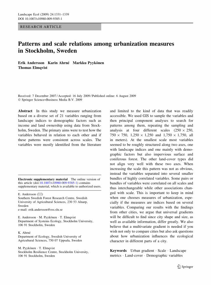
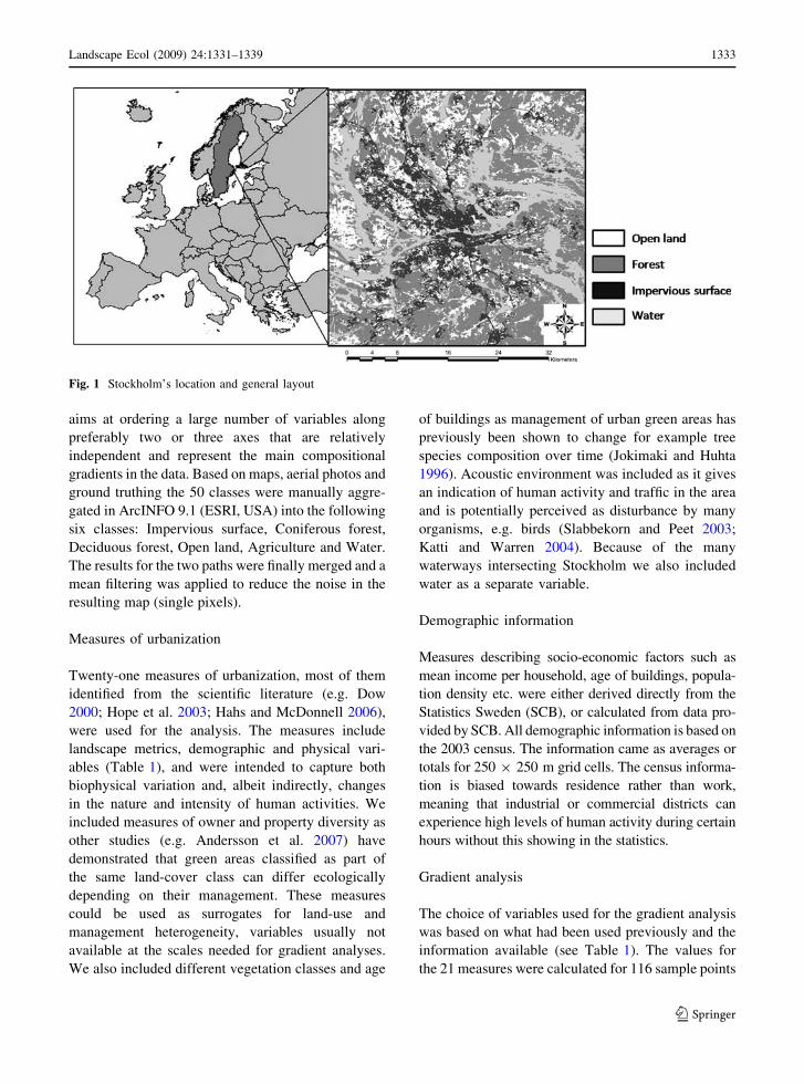
Our study was carried out in the city of Stockholm,

Sweden’s capital and largest urbanized area, located at

59�200N latitude and 18�050E longitude on the eastern

coast (Fig. 1). The city core straddles Lake Malaren’s

outlet into the Baltic Sea, and the city is characterized

by many waterways and a relatively high proportion of

green areas. The Stockholm County today houses

approximately 1.8 million people (SCB 2006), a figure

expected to increase by 200,000 over the next 10 years

(RTK 2005). Development has followed several

different planning paradigms over time, thus adding

to the overall heterogeneity (cf. Elmqvist et al. 2004;

Barthel et al. 2005).

Creating a land-cover map based on satellite

images

Due to lack of a uniform land-cover map over the

whole Stockholm Metropolitan area, satellite imagery

was used to create a map containing the six dominating

land-cover types within the study area. The classifica-

tion was based on three SPOT 5 satellite images with

10 m resolution. The images are from 3 August and 12

August 2004 with GRS IDs K/J 061/228, 058/228 and

061/229 respectively (Metria 2006). Since the two

paths are from different dates the images from each

path were classified independently. A principal com-

ponent analysis (PCA) was performed, followed by an

unsupervised classification in ERDAS 9.0 (Leica

Geosystems Geospatial Imaging, USA) generating

50 classes based on the digital numbers (Lillesand

et al. 2003). The PCA is a linear ordination method that

1332 Landscape Ecol (2009) 24:1331–1339

123

aims at ordering a large number of variables along

preferably two or three axes that are relatively

independent and represent the main compositional

gradients in the data. Based on maps, aerial photos and

ground truthing the 50 classes were manually aggre-

gated in ArcINFO 9.1 (ESRI, USA) into the following

six classes: Impervious surface, Coniferous forest,

Deciduous forest, Open land, Agriculture and Water.

The results for the two paths were finally merged and a

mean filtering was applied to reduce the noise in the

resulting map (single pixels).

Measures of urbanization

Twenty-one measures of urbanization, most of them

identified from the scientific literature (e.g. Dow

2000; Hope et al. 2003; Hahs and McDonnell 2006),

were used for the analysis. The measures include

landscape metrics, demographic and physical vari-

ables (Table 1), and were intended to capture both

biophysical variation and, albeit indirectly, changes

in the nature and intensity of human activities. We

included measures of owner and property diversity as

other studies (e.g. Andersson et al. 2007) have

demonstrated that green areas classified as part of

the same land-cover class can differ ecologically

depending on their management. These measures

could be used as surrogates for land-use and

management heterogeneity, variables usually not

available at the scales needed for gradient analyses.

We also included different vegetation classes and age

of buildings as management of urban green areas has

previously been shown to change for example tree

species composition over time (Jokimaki and Huhta

1996). Acoustic environment was included as it gives

an indication of human activity and traffic in the area

and is potentially perceived as disturbance by many

organisms, e.g. birds (Slabbekorn and Peet 2003;

Katti and Warren 2004). Because of the many

waterways intersecting Stockholm we also included

water as a separate variable.

Demographic information

Measures describing socio-economic factors such as

mean income per household, age of buildings, popula-

tion density etc. were either derived directly from the

Statistics Sweden (SCB), or calculated from data pro-

vided by SCB. All demographic information is based on

the 2003 census. The information came as averages or

totals for 250 9 250 m grid cells. The census informa-

tion is biased towards residence rather than work,

meaning that industrial or commercial districts can

experience high levels of human activity during certain

hours without this showing in the statistics.

Gradient analysis

The choice of variables used for the gradient analysis

was based on what had been used previously and the

information available (see Table 1). The values for

the 21 measures were calculated for 116 sample points

Fig. 1 Stockholm’s location and general layout

Landscape Ecol (2009) 24:1331–1339 1333

123

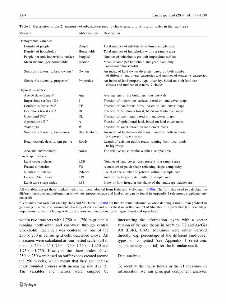
within two transects with 1,750 9 1,750 m grid cells

running north-south and east-west through central

Stockholm. Each cell was centered on one of the

250 9 250 m census grid cells described above. All

measures were calculated at four nested scales (all in

meters), 250 9 250, 750 9 750, 1,250 9 1,250 and

1,750 9 1,750. However, the three scales above

250 9 250 were based on buffer zones created around

the 250 m cells, which meant that they got increas-

ingly rounded corners with increasing size (Fig. 2).

The variables and metrics were sampled by

intersecting the information layers with a vector

version of the grid theme in ArcView 3.2 and ArcGis

9.0 (ESRI, USA). Measures were either derived

directly, e.g. percentage of the different land-cover

types, or computed (see Appendix 1 (electronic

supplementary material) for the formulae used).

Data analysis

To identify the major trends in the 21 measures of

urbanization we ran principal component analyses

Table 1 Description of the 21 measures of urbanization used to characterize grid cells at all scales in the study area

Measure Abbreviations Description

Demographic variables

Density of people People Total number of inhabitants within a sample area

Density of households Households Total number of households within a sample area

People per unit impervious surface People/I Number of inhabitants per unit impervious surface

Mean income (per household)a Income Mean income per household and year, excluding

no-income households

Simpson’s diversity, land ownersa Owners An index of land owner diversity, based on both number

of different land owner categories and number of estates, 8 categories

Simpson’s diversity, propertiesa Properties An index of land property type diversity, based on both land-use

classes and number of estates, 7 classes

Physical variables

Age of developmenta Age Average age of the buildings, four intervals

Impervious surface (%) I Fraction of impervious surface, based on land-cover maps

Coniferous forest (%)a CF Fraction of coniferous forest, based on land-cover maps

Deciduous forest (%)a DF Fraction of deciduous forest, based on land-cover maps

Open land (%)a OL Fraction of open land, based on land-cover maps

Agriculture (%)a A Fraction of agricultural land, based on land-cover maps

Water (%) W Fraction of water, based on land-cover maps

Simpson’s diversity, land-cover Div. land-cov. An index of land-cover diversity, based on both richness

and proportion, 6 classes

Road network density, km per ha Roads Length of existing public roads, ranging from local roads

to highways

Acoustic environmenta Noise The relative noise profile within a sample area

Landscape metrics

Land-cover richness LCR Number of land-cover types present in a sample area

Fractal dimension FD A measure of patch shape reflecting shape complexity

Number of patches Patches Count of the number of patches within a sample area

Largest Patch Index LPI Area of the largest patch within a sample area

Landscape shape index LSI Index of how irregular the shape of the landscape patches are

All variables except those marked with a star were adopted from Hahs and McDonnell (2006). The formulae used to calculate the

different measures and information on owners, properties, age and land-cover can be found in Appendix 1 (electronic supplementary

material)a Variables that were not used by Hahs and McDonnell (2006) but that we found informative when defining a rural-urban gradient in

general (i.e. acoustic environment, diversity of owners and properties) or in the context of Stockholm in particular (i.e. percentage

impervious surface including water, deciduous and coniferous forest, agricultural and open land)

1334 Landscape Ecol (2009) 24:1331–1339

123

(PCA) at each scale. The data was first standardized

using ‘center and standardize by species’, which is an

option suitable for variables that are measured in

different units (ter Braak and Smilauer 2002). By

standardizing, we gave all variables the same varia-

tion, i.e. a standard deviation of 1. The data for the

four different scales were analyzed separately to find

out how the relation between variables would change

with increasing spatial scale.

Results

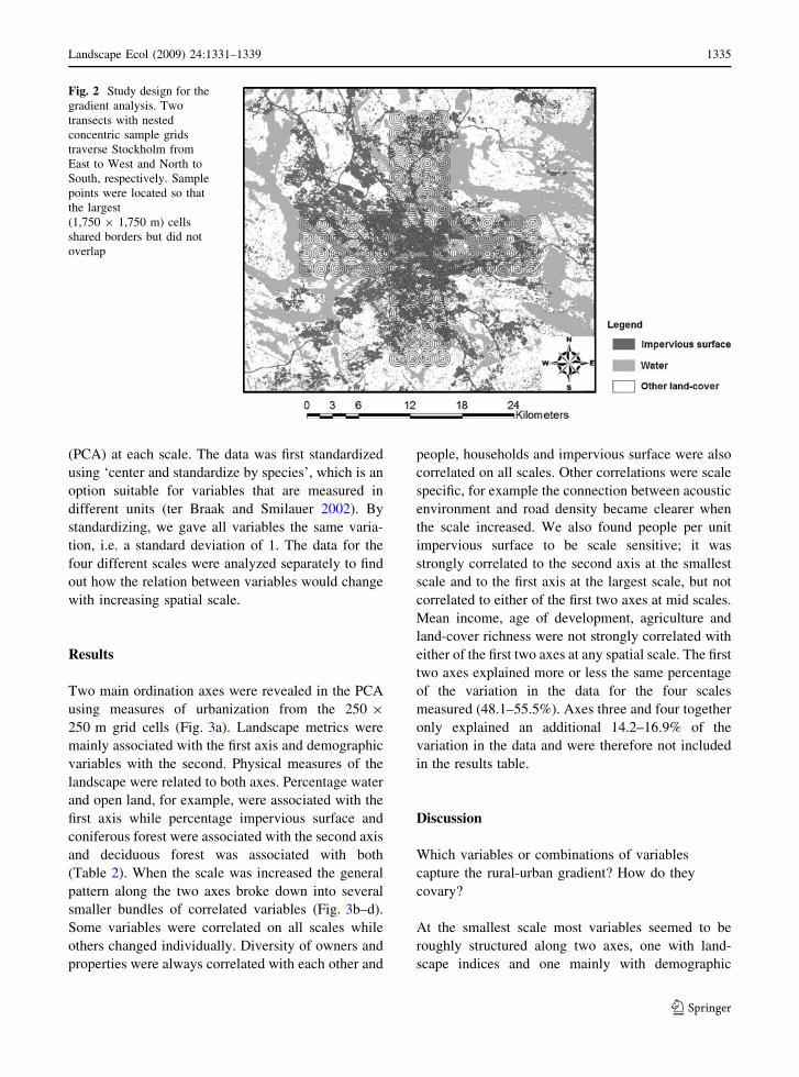
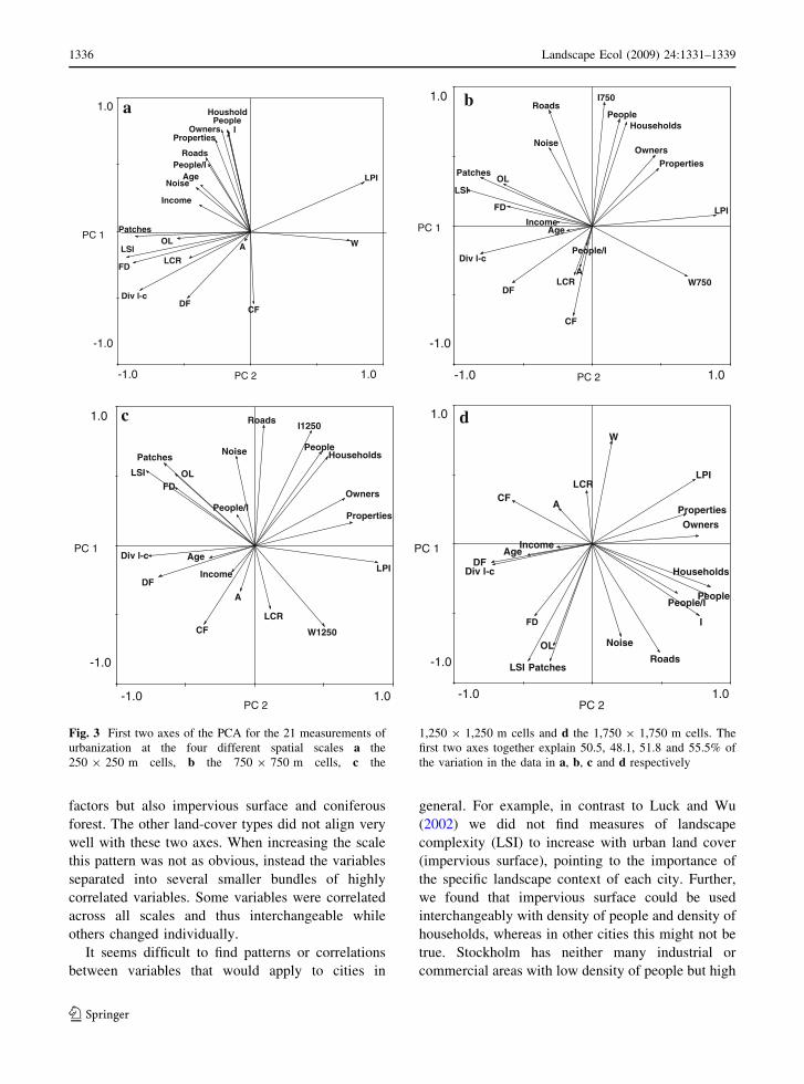
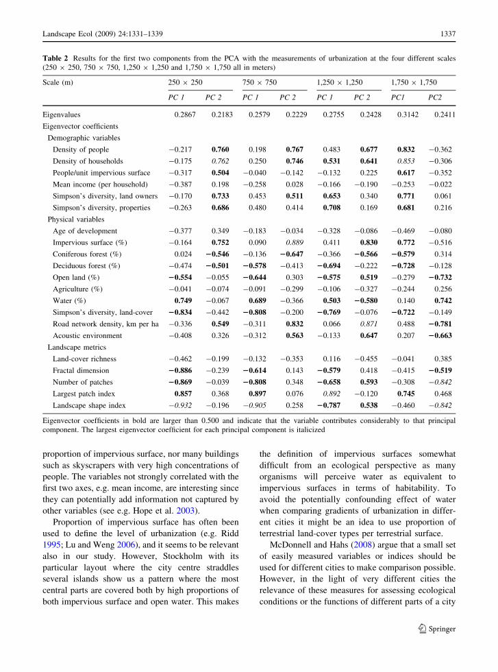
Two main ordination axes were revealed in the PCA

using measures of urbanization from the 250 9

250 m grid cells (Fig. 3a). Landscape metrics were

mainly associated with the first axis and demographic

variables with the second. Physical measures of the

landscape were related to both axes. Percentage water

and open land, for example, were associated with the

first axis while percentage impervious surface and

coniferous forest were associated with the second axis

and deciduous forest was associated with both

(Table 2). When the scale was increased the general

pattern along the two axes broke down into several

smaller bundles of correlated variables (Fig. 3b–d).

Some variables were correlated on all scales while

others changed individually. Diversity of owners and

properties were always correlated with each other and

people, households and impervious surface were also

correlated on all scales. Other correlations were scale

specific, for example the connection between acoustic

environment and road density became clearer when

the scale increased. We also found people per unit

impervious surface to be scale sensitive; it was

strongly correlated to the second axis at the smallest

scale and to the first axis at the largest scale, but not

correlated to either of the first two axes at mid scales.

Mean income, age of development, agriculture and

land-cover richness were not strongly correlated with

either of the first two axes at any spatial scale. The first

two axes explained more or less the same percentage

of the variation in the data for the four scales

measured (48.1–55.5%). Axes three and four together

only explained an additional 14.2–16.9% of the

variation in the data and were therefore not included

in the results table.

Discussion

Which variables or combinations of variables

capture the rural-urban gradient? How do they

covary?

At the smallest scale most variables seemed to be

roughly structured along two axes, one with land-

scape indices and one mainly with demographic

Fig. 2 Study design for the

gradient analysis. Two

transects with nested

concentric sample grids

traverse Stockholm from

East to West and North to

South, respectively. Sample

points were located so that

the largest

(1,750 9 1,750 m) cells

shared borders but did not

overlap

Landscape Ecol (2009) 24:1331–1339 1335

123

factors but also impervious surface and coniferous

forest. The other land-cover types did not align very

well with these two axes. When increasing the scale

this pattern was not as obvious, instead the variables

separated into several smaller bundles of highly

correlated variables. Some variables were correlated

across all scales and thus interchangeable while

others changed individually.

It seems difficult to find patterns or correlations

between variables that would apply to cities in

general. For example, in contrast to Luck and Wu

(2002) we did not find measures of landscape

complexity (LSI) to increase with urban land cover

(impervious surface), pointing to the importance of

the specific landscape context of each city. Further,

we found that impervious surface could be used

interchangeably with density of people and density of

households, whereas in other cities this might not be

true. Stockholm has neither many industrial or

commercial areas with low density of people but high

-1.0 1.0

-1.0

1.0

I

W

Div l-c

LCR

PeopleHoushold

People/I

Income

OwnersProperties

Roads

Noise

FD

Patches

LPI

LSI

Age

OLA

DFCF

PC 2

PC 1

0.10.1-

-1.0

1.0 I750

W750

Div l-c

LCR

PeopleHouseholds

People/I

Income

OwnersProperties

Roads

Noise

FD

Patches

LPI

LSI

Age

OL

A

DF

CF

PC 2

PC 1

-1.0 1.0

-1.0

1.0I1250

W1250

Div l-c

LCR

PeopleHouseholds

People/I

Income

Owners

Properties

Roads

Noise

FD

Patches

LPI

LSI

Age

OL

A

DF

CF

PC 2

PC 1

0.10.1-

-1.0

1.0

I

W

Div l-c

LCR

People

Households

People/I

Income

OwnersProperties

Roads

Noise

FD

Patches

LPI

LSI

Age

OL

A

DF

CF

PC 2

PC 1

a b

dc

Fig. 3 First two axes of the PCA for the 21 measurements of

urbanization at the four different spatial scales a the

250 9 250 m cells, b the 750 9 750 m cells, c the

1,250 9 1,250 m cells and d the 1,750 9 1,750 m cells. The

first two axes together explain 50.5, 48.1, 51.8 and 55.5% of

the variation in the data in a, b, c and d respectively

1336 Landscape Ecol (2009) 24:1331–1339

123

proportion of impervious surface, nor many buildings

such as skyscrapers with very high concentrations of

people. The variables not strongly correlated with the

first two axes, e.g. mean income, are interesting since

they can potentially add information not captured by

other variables (see e.g. Hope et al. 2003).

Proportion of impervious surface has often been

used to define the level of urbanization (e.g. Ridd

1995; Lu and Weng 2006), and it seems to be relevant

also in our study. However, Stockholm with its

particular layout where the city centre straddles

several islands show us a pattern where the most

central parts are covered both by high proportions of

both impervious surface and open water. This makes

the definition of impervious surfaces somewhat

difficult from an ecological perspective as many

organisms will perceive water as equivalent to

impervious surfaces in terms of habitability. To

avoid the potentially confounding effect of water

when comparing gradients of urbanization in differ-

ent cities it might be an idea to use proportion of

terrestrial land-cover types per terrestrial surface.

McDonnell and Hahs (2008) argue that a small set

of easily measured variables or indices should be

used for different cities to make comparison possible.

However, in the light of very different cities the

relevance of these measures for assessing ecological

conditions or the functions of different parts of a city

Table 2 Results for the first two components from the PCA with the measurements of urbanization at the four different scales

(250 9 250, 750 9 750, 1,250 9 1,250 and 1,750 9 1,750 all in meters)

Scale (m) 250 9 250 750 9 750 1,250 9 1,250 1,750 9 1,750

PC 1 PC 2 PC 1 PC 2 PC 1 PC 2 PC1 PC2

Eigenvalues 0.2867 0.2183 0.2579 0.2229 0.2755 0.2428 0.3142 0.2411

Eigenvector coefficients

Demographic variables

Density of people -0.217 0.760 0.198 0.767 0.483 0.677 0.832 -0.362

Density of households -0.175 0.762 0.250 0.746 0.531 0.641 0.853 -0.306

People/unit impervious surface -0.317 0.504 -0.040 -0.142 -0.132 0.225 0.617 -0.352

Mean income (per household) -0.387 0.198 -0.258 0.028 -0.166 -0.190 -0.253 -0.022

Simpson’s diversity, land owners -0.170 0.733 0.453 0.511 0.653 0.340 0.771 0.061

Simpson’s diversity, properties -0.263 0.686 0.480 0.414 0.708 0.169 0.681 0.216

Physical variables

Age of development -0.377 0.349 -0.183 -0.034 -0.328 -0.086 -0.469 -0.080

Impervious surface (%) -0.164 0.752 0.090 0.889 0.411 0.830 0.772 -0.516

Coniferous forest (%) 0.024 20.546 -0.136 20.647 -0.366 20.566 20.579 0.314

Deciduous forest (%) -0.474 20.501 20.578 -0.413 20.694 -0.222 20.728 -0.128

Open land (%) 20.554 -0.055 20.644 0.303 20.575 0.519 -0.279 20.732

Agriculture (%) -0.041 -0.074 -0.091 -0.299 -0.106 -0.327 -0.244 0.256

Water (%) 0.749 -0.067 0.689 -0.366 0.503 20.580 0.140 0.742

Simpson’s diversity, land-cover 20.834 -0.442 20.808 -0.200 20.769 -0.076 20.722 -0.149

Road network density, km per ha -0.336 0.549 -0.311 0.832 0.066 0.871 0.488 20.781

Acoustic environment -0.408 0.326 -0.312 0.563 -0.133 0.647 0.207 20.663

Landscape metrics

Land-cover richness -0.462 -0.199 -0.132 -0.353 0.116 -0.455 -0.041 0.385

Fractal dimension 20.886 -0.239 20.614 0.143 20.579 0.418 -0.415 20.519

Number of patches 20.869 -0.039 20.808 0.348 20.658 0.593 -0.308 -0.842

Largest patch index 0.857 0.368 0.897 0.076 0.892 -0.120 0.745 0.468

Landscape shape index -0.932 -0.196 -0.905 0.258 20.787 0.538 -0.460 -0.842

Eigenvector coefficients in bold are larger than 0.500 and indicate that the variable contributes considerably to that principal

component. The largest eigenvector coefficient for each principal component is italicized

Landscape Ecol (2009) 24:1331–1339 1337

123

seems rather dubious (cf. ibid). Finding these broad

measures, e.g. different indices (Hahs and McDonnell

2006), can be difficult for several reasons. First,

combining demographic and landscape information

can be problematic. We did not have access to data

with the same resolution for all our measurements

and data availability and quality are likely to vary a

great deal between cities and countries. For some of

the variables we have detailed information while for

others, e.g. for acoustic environment and mean

income, we have used average values. Second,

finding a generic classification of land-cover seems

unlikely, especially when there are problems with

measuring even a class as well-defined as impervious

surface (Lu and Weng 2006). We divided the land-

cover data into six classes and even though we

distinguished between deciduous and coniferous

forest it would have been interesting to divide the

urban green areas even further, according to man-

agement. Third, the availability of data will differ

substantially between cities. For example, included

among the measures proposed by McDonnell and

Hahs (2008) was an index based on information that,

at least for Stockholm, was not readily available (e.g.

number of males in non-agricultural jobs). One of the

ideas with our study was to find variables that were

both relevant as measures of urbanization and

relatively easy to find information about. Therefore

some of the social variables such as local green area

management, a variable truly important for many

organisms (e.g. Andersson et al. 2007), were not

possible to include. Nevertheless, we believe that a

diverse set of variables would allow comparisons as

well as practical use in planning.

Spatial scales

The importance and effect of scale will vary between

cities; Stockholm is rather small and has through its

system of green wedges access to large green areas

even close to the city center. The grain and extent on

different patterns is generally accepted to influence

the analysis (e.g. Wiens 1989; Gustafson 1998; Wu

2004). However, within the growing literature on

urban gradients few articles address the variables of

urbanization (McDonnell and Hahs 2008), and fewer

still test the importance of the analytical scale (Wu

et al. 2002). Our set-up explicitly tested the effect of

scale and whether the relationship between variables

changed with scale. The results suggest that correla-

tions change with scale; some variables can be used

interchangeably across scales while other display

similar behavior only on certain scales. Thus, scale

dependence both in variable behavior and potentially

in relative importance call for multi-scaled gradients.

McDonnell and Hahs (2008) argue for the use of

indices to define urbanization. From looking at our

results we see a potential problem in the interpreta-

tion of the indices if the variables used for calculation

would prove to have scale specific behavior. Also, it

is interesting to see that the landscape metrics

strongly correlated with axis 1 at the smallest scale

change their affiliation to axis 2 at the largest scale,

and vice versa for some of the demographic variables.

While measuring several variables we measured

all of them across all scales. In our choice of

commonly used variables we might have missed

variables that are only relevant at certain scales.

Landscape studies aimed at understanding patterns of

species occurrence in cities have frequently showed

that qualitatively different sets of variables are

relevant at different scales (e.g. Whited et al. 2000;

Melles et al. 2003). However, considering the lack of

city wide information on local conditions in terms of

e.g. vegetation structure and management activities

we see such information as a necessary complement

to but not part of future gradient analyses.

Conclusions

Differences between measures used to characterize

urbanization were in our case clearest at a small

scale, where variable behavior could largely be

explained by two general axes. We found that

variables covary, but not consistently across scales.

This is important to keep in mind when one chooses

measures of urbanization, especially if the measures

are indices based on several variables. We believe

that a multivariate gradient is needed if you wish not

only to compare cities but also ask questions about

how urbanization influences the ecological character

in different parts of a city.

Acknowledgment We thank Jan Bengtsson and Asa

Berggren for valuable comments on earlier versions of the

manuscript. Funding was provided by the Swedish Research

Council and Formas.

1338 Landscape Ecol (2009) 24:1331–1339

123

References

Andersson E, Barthel S, Ahrne K (2007) Measuring social-

ecological dynamics behind the generation of ecosystem

services. Ecol Appl 17:1267–1278

Barthel S, Colding J, Elmqvist T, Folke C (2005) History and

local management of a biodiversity-rich, urban, cultural

landscape. Ecol Soc 10:10

Blair RB (1996) Land use and avian species diversity along an

urban gradient. Ecol Appl 6:506–519

Bowers MA, Breland B (1996) Foraging of gray squirrels on an

urban—rural gradient: use of the GUD to assess anthro-

pogenic impact. Ecol Appl 6:1135–1142

Burton E, Weich S, Blanchard M, Prince M (2005) Measuring

physical characteristics of housing: the Built Environment

Site Survey Checklist (BESSC). Environ Plann B Plann

Des 32:265–280

Cadenasso ML, Pickett STA, Schwarz K (2007) Spatial het-

erogeneity in urban ecosystems: reconceptualizing land

cover and a framework for classification. Frontiers Ecol

Environ 5:80–88

Carreiro MM, Howe K, Parkhurst DF, Pouyat RV (1999)

Variation in quality and decomposability of red oak leaf

litter along an urban–rural gradient. Biol Fertil Soils

30:258–268

Collins JP, Kinzig A, Grimm NB, Fagan WF, Hope D, Wu J,

Borer ET (2000) A new urban ecology—modeling human

communities as integral parts of ecosystems poses special

problems for the development and testing of ecological

theory. American Sci 88:416–425

Dow K (2000) Social dimensions of gradients in urban eco-

systems. Urban Ecosyst 4:255–275

Elmqvist T, Colding J, Barthel S, Borgstrom S, Duit A,

Lundberg J, Andersson E, Ahrne K, Ernstson H, Folke C,

Bengtsson J (2004) The dynamics of social-ecological

systems in urban landscapes—Stockholm and the

National Urban Park, Sweden. In: Alfsen-Norodom C,

Lane BD, Corry M (eds) Urban biosphere and society:

partnership of cities. Annals of the New York Academy of

Sciences, New York, pp 308–322

Germaine SS, Wakeling BF (2001) Lizard species distributions

and habitat occupation along an urban gradient in Tucson,

Arizona, USA. Biol Conserv 97:229–237

Gustafson EJ (1998) Quantifying landscape spatial pattern:

what is the state of the art? Ecosystems 1:143–156

Hahs AK, McDonnell MJ (2006) Selecting independent mea-

sures to quantify Melbourne’s urban–rural gradient.

Landsc Urban Plann 78:435–448

Hope D, Gries C, Zhu WX, Fagan WF, Redman CL, Grimm

NB, Nelson AL, Martin C, Kinzig A (2003) Socioeco-

nomics drive urban plant diversity. Proc Natl Acad Sci

USA 100:8788–8792

Jokimaki J, Huhta E (1996) Effects of landscape matrix and

habitat structure on a bird community in northern Finland:

a multi-scale approach. Ornis Fennica 73:97–113

Katti M, Warren PS (2004) Tits, noise and urban bioacoustics.

Trends Ecol Evol 19:109–110

Kinzig AP, Warren P, Martin C, Hope D, Katti M (2005) The

effects of human socioeconomic status and cultural

characteristics on urban patterns of biodiversity. Ecol Soc

10:23

Levin SA (1992) The problem of pattern and scale in ecology.

Ecology 73:1943–1967

Lillesand TM, Kiefer RW, Chipman JW (2003) Remote

sensing and image interpretation. Wiley, New York

Lu D, Weng Q (2006) Use of impervious surface in urban land-

use classification. Remote Sens Environ 102:146–160

Luck M, Wu JG (2002) A gradient analysis of urban landscape

pattern: a case study from the Phoenix metropolitan

region, Arizona, USA. Landscape Ecol 17:327–339

McDonnell MJ, Hahs AK (2008) The use of gradient analysis

studies in advancing our understanding of the ecology of

urbanizing landscapes: current status and future direc-

tions. Landscape Ecol 23:1143–1155

McDonnell MJ, Pickett STA (1990) Ecosystem structure and

function along urban rural gradients—an unexploited

opportunity for ecology. Ecology 71:1232–1237

McIntyre NE, Knowles-Yanez K, Hope D (2000) Urban

ecology as an interdisciplinary field: differences in the use

of ‘‘urban’’ between the social and natural sciences. Urban

Ecosyst 4:5–24

Melles S, Glenn S, Martin K (2003) Urban bird diversity and

landscape complexity: species-environment associations

along a multiscale habitat gradient. Conserv Ecol 7:5

Metria (2006) Spot CNES 2006. Swedish Land Survey,

Sweden

Ridd MK (1995) Exploring a V-I-S (vegetation-impervious

surface-soil) model for urban ecosystem analysis through

remote sensing: comparative anatomy for cities. Int J

Remote Sens 16:2165–2185

RTK (2005) Befolkningsprognos 2005 for perioden 2005–2014,

Stockholm, p 69

SCB (2006) Statistical yearbook of Sweden. Statistics Sweden

Slabbekorn H, Peet M (2003) Birds sing at a higher pitch in

urban noise. Nature 424:267

Steffan-Dewenter I, Munzenberg U, Burger C, Thies C,

Tscharntke T (2002) Scale-dependent effects of landscape

context on three pollinator guilds. Ecology 83:1421–1432

ter Braak CJF, Smilauer P (2002) CANOCO reference manual

and CanoDraw for Windows User’s guide: software for

Canonical Community Ordination (version 4.5). Micro-

computer Power. Ithaca, NY

Whited D, Galatowitsch S, Tester JR, Schik K, Lehtinen R,

Husveth J (2000) The importance of local and regional

factors in predicting effective conservation—planning

strategies for wetland bird communities in agricultural

and urban landscapes. Landsc Urban Plann 49:49–65

Whittaker RH (1967) Gradient analysis of vegetation. Biol Rev

42:207–264

Wiens JA (1989) Spatial scaling in ecology. Funct Ecol 3:

385–397

Wu J (2004) Effects of changing scale on landscape pattern

analysis: scaling relations. Landscape Ecol 19:125–138

Wu J, Shen W, Sun W, Tueller PT (2002) Empirical patterns of

the effects of changing scale on landscape metrics.

Landscape Ecol 17:761–782

Landscape Ecol (2009) 24:1331–1339 1339

123