Embed Size (px)
Citation preview
Pattern Matching and Detection in
Extremely Resource Constrained
Wireless Sensor Networks
Michael Zoumboulakis
May 2011
A Dissertation Submitted to
Birkbeck College, University of London
in Partial Fulfillment of the Requirements
for the Degree of Doctor of Philosophy
School of Computer Science & Information Systems
Birkbeck College
University of London

Declaration
This thesis is the result of my own work, except where explicitly acknowledged
in the text.
Michael Zoumboulakis
May 8, 2011
Abstract
This thesis investigates the problem of pattern matching and detection in ex-
tremely resource constrained Wireless Sensor Networks (WSNs). Specifically, it
introduces a collection of in-network methods and algorithms which exploit the
observation that processing data inside the network, instead of transmitting it off-
network, offers a distinct advantage for sensor node longevity through reduction
of network communication.
Operating on windowed sensor observations, we develop temporal domain
algorithms that apply symbolic conversion and examine the resulting strings
for interesting or unusual patterns with a choice of exact, approximate, non-
parametric, probabilistic and multiple pattern matching and detection methods.
Precise implementation of the algorithms with integer-only arithmetic, results
into a computationally efficient execution profile and modest RAM requirements.
Furthermore, we develop a spatial pattern event location estimation algorithm
that combines a geometric method with the application of the Kalman filter to
iteratively compute an estimate of the pattern event source location and intensity.
This algorithm is decentralised and operates by tasking WSN nodes to collaborate
by exchanging information with local neighbours in order to improve estimate
accuracy with respect to location and intensity of the spatial pattern event source.
We provide evidence that the proposed algorithms are competitive against
alternative methods and validate their operational performance through deploy-
ment on WSN nodes and simulations. Overall, we find the proposed algorithms
support reactive behaviour in the case of WSNs and align well with the generic
goal of preserving resources.
3

To my parents
4

Acknowledgements
I owe my deepest gratitude to my supervisor Dr. George Roussos whose en-
couragement, guidance and support enabled me to gain a deep understanding
of Wireless Sensor Networks and Ubiquitous Computing. I am also indebted
to my second supervisor Prof. Alexandra Poulovassilis for steering my research
and providing valuable feedback. Dr. Eleftheria Katsiri deserves special thanks
and credit for the idea of an efficient Integer-only Complex Event Detection im-
plementation. I am grateful to Prof. Eamonn Keogh for patiently answering
questions about Symbolic Aggregate Approximation and providing relevant test
data. I would like to extend my gratitude to Dr. Nigel Martin who provided the
valuable support for this research.
On a personal level, my warmest thanks go to my parents and my two sisters
whose unconditional love and support made this thesis possible. I am grateful
to my Knowledge Lab colleagues Dimitrios Airantzis, Lucas Zamboulis, Rajesh
Pampapathi and Jenson Taylor for their help and friendship. Marco Luchini
deserves special thanks for financing part of my research in return for (sometimes
frightening) work on critical systems. Finally, I am indebted to my friends Vassili,
Vasso, Michael, Jack and Helge for their friendship and support throughout the
process.
5
Contents
Abstract 3
Acknowledgements 5
1 Introduction 14
1.1 Overview and Motivation . . . . . . . . . . . . . . . . . . . . . . . 14
1.1.1 WSN Constraints and Challenges . . . . . . . . . . . . . . 15
1.1.2 Definitions . . . . . . . . . . . . . . . . . . . . . . . . . . . 17
1.2 Research Methodology . . . . . . . . . . . . . . . . . . . . . . . . 18
1.2.1 Requirements and Research Questions . . . . . . . . . . . 18
1.2.2 Research Methods . . . . . . . . . . . . . . . . . . . . . . 19
1.3 Contributions . . . . . . . . . . . . . . . . . . . . . . . . . . . . . 20
1.4 Assumptions and Limitations . . . . . . . . . . . . . . . . . . . . 21
1.5 Outline of the Thesis . . . . . . . . . . . . . . . . . . . . . . . . . 22
2 Pattern Matching and Detection in WSNs and Sensor Data 23
2.1 Environmental Monitoring . . . . . . . . . . . . . . . . . . . . . . 24
2.2 Data Centre and Structural Monitoring . . . . . . . . . . . . . . . 25
2.3 Body Sensor Networks and Context Aware Systems . . . . . . . . 26
2.4 Network Monitoring and Security . . . . . . . . . . . . . . . . . . 28
2.5 Spacecraft and Telemetry Pattern Classification . . . . . . . . . . 30
2.6 Spatial Pattern Location Estimation . . . . . . . . . . . . . . . . 30
2.7 Generic Approaches and Additional Applications . . . . . . . . . 32
2.8 Summary . . . . . . . . . . . . . . . . . . . . . . . . . . . . . . . 34
6
3 Pattern Matching and Detection in the Temporal Domain 37
3.1 The Basis for Pattern Matching and Detection . . . . . . . . . . . 37
3.1.1 Advantages of Symbolic Transformation . . . . . . . . . . 38
3.1.2 An Overview of Symbolic Aggregate Approximation . . . . 40
3.1.3 Assessing Pattern Similarity and Probability . . . . . . . . 42
3.2 Exact and Approximate Pattern Matching . . . . . . . . . . . . . 43
3.3 Multiple Pattern Matching . . . . . . . . . . . . . . . . . . . . . . 44
3.4 Non-Parametric Pattern Detection . . . . . . . . . . . . . . . . . 46
3.5 Probabilistic Pattern Detection . . . . . . . . . . . . . . . . . . . 46
3.6 Summary . . . . . . . . . . . . . . . . . . . . . . . . . . . . . . . 48
4 Temporal Algorithms: Evaluation through Emulation 50
4.1 Methodology and Experimental Setup . . . . . . . . . . . . . . . . 50
4.2 Case Study 1: Indoor Deployment . . . . . . . . . . . . . . . . . . 52
4.2.1 Evaluation of Exact and Approximate Matching . . . . . . 52
4.3 Case Study 2: Seismic and Acoustic Data . . . . . . . . . . . . . 58
4.3.1 Evaluation of Non-Parametric Pattern Detection . . . . . . 58
4.3.2 The Effect of Measurement Noise to NPPD . . . . . . . . 64
4.4 Case Study 3: Physiological Data . . . . . . . . . . . . . . . . . . 66
4.4.1 Evaluation of NPPD and PPD . . . . . . . . . . . . . . . . 67
4.5 Summary of Findings . . . . . . . . . . . . . . . . . . . . . . . . . 72
5 Temporal Algorithms: Evaluation through Deployment 73
5.1 Execution Profile of Temporal Domain Algorithms . . . . . . . . . 73
5.1.1 Refactoring of Pattern Matching and Detection Algorithms 74
5.2 Dynamic Sampling Frequency Management (DSFM) Algorithm . 81
5.2.1 Data Centre WSN Deployment . . . . . . . . . . . . . . . 83
5.3 Integration with Publish/Subscribe . . . . . . . . . . . . . . . . . 90
5.4 Observations from Further Deployments . . . . . . . . . . . . . . 91
5.5 Summary of Findings . . . . . . . . . . . . . . . . . . . . . . . . . 92
7

6 Pattern Location Estimation in the Spatial Domain 94
6.1 The Location Estimation Problem . . . . . . . . . . . . . . . . . . 94
6.2 Kalman Filter Properties . . . . . . . . . . . . . . . . . . . . . . . 95
6.3 Spatial Pattern Location Estimation (SPLE) Algorithm . . . . . . 98
6.4 Summary . . . . . . . . . . . . . . . . . . . . . . . . . . . . . . . 103
7 Spatial Algorithm: Evaluation through Simulation 104
7.1 Methodology and Simulation Set-up . . . . . . . . . . . . . . . . . 104
7.1.1 Maximum Selection Algorithm . . . . . . . . . . . . . . . . 105
7.1.2 Dispersion Model . . . . . . . . . . . . . . . . . . . . . . . 105
7.1.3 Kalman Filter Initial Parameters . . . . . . . . . . . . . . 106
7.1.4 Topology Generation . . . . . . . . . . . . . . . . . . . . . 107
7.2 Evaluation of Spatial Pattern Location Estimation . . . . . . . . . 108
7.2.1 Metrics . . . . . . . . . . . . . . . . . . . . . . . . . . . . 108
7.2.2 Grid Topology . . . . . . . . . . . . . . . . . . . . . . . . . 108
7.2.3 Random Topology . . . . . . . . . . . . . . . . . . . . . . 110
7.3 Summary of Findings . . . . . . . . . . . . . . . . . . . . . . . . . 114
8 Conclusions and Future Work 118
8.1 Summary of the Thesis . . . . . . . . . . . . . . . . . . . . . . . . 118
8.2 Summary of Contributions . . . . . . . . . . . . . . . . . . . . . . 121
8.3 Critical Appraisal . . . . . . . . . . . . . . . . . . . . . . . . . . . 122
8.4 Directions for Future Research . . . . . . . . . . . . . . . . . . . . 122
Bibliography 129
A Publications 147
B Example of Multiple Pattern Matching 149
C Software Development Timing Model 152
D Maximum Selection Spatial Location Algorithm 154
8
List of Figures
1.1 Typical WSN nodes: TMote Sky and TI ez430-rf2500 . . . . . . . 16
1.2 Power draw of a TMote Sky . . . . . . . . . . . . . . . . . . . . . 17
3.1 Scale-independent pattern matching example . . . . . . . . . . . . 39
3.2 Symbolic conversion example . . . . . . . . . . . . . . . . . . . . . 41
4.1 Emulating data acquisition in MATLAB . . . . . . . . . . . . . . 51
4.2 Case study 1: APM example . . . . . . . . . . . . . . . . . . . . . 57
4.3 Case study 2: NPPD example . . . . . . . . . . . . . . . . . . . . 62
4.4 Case study 2: NPPD compared to EWMA . . . . . . . . . . . . . 63
4.4 Case study 2: NPPD compared to RSAM . . . . . . . . . . . . . 64
4.5 Case study 2: Impact of signal noise to NPPD . . . . . . . . . . . 66
4.6 Case study 3: NPPD example on ECG data . . . . . . . . . . . . 70
4.7 Case study 3: PPD example on EMG data . . . . . . . . . . . . . 71
5.1 APM/EPM Runtime comparison . . . . . . . . . . . . . . . . . . 79
5.2 Runtime comparison of MPM and Linear Search. . . . . . . . . . 80
5.3 Node locations from data centre deployment . . . . . . . . . . . . 85
5.4 DC deployment: detected patterns . . . . . . . . . . . . . . . . . 89
6.1 The Kalman filter loop . . . . . . . . . . . . . . . . . . . . . . . . 96
6.2 Estimate propagation example . . . . . . . . . . . . . . . . . . . . 101
6.3 Example of the SPLE geometric computation . . . . . . . . . . . 102
7.1 Dispersion plume and concentration intensities . . . . . . . . . . . 110
9

7.2 Geometric computation example (a) . . . . . . . . . . . . . . . . . 115
7.2 Geometric computation example (b) . . . . . . . . . . . . . . . . 116
7.2 Geometric computation example (c) . . . . . . . . . . . . . . . . . 117
10

List of Tables
2.1 Comparison of alternative event detection methods . . . . . . . . 35
2.1 Comparison of alternative event detection methods (cont’d) . . . 36
3.1 Sample distance lookup table for 10-letter alphabet . . . . . . . . 42
4.1 Mean number of false positives for APM Algorithm . . . . . . . . 55
4.2 Mean number of false positives for EPM Algorithm . . . . . . . . 56
4.3 NPPD performance compared to EWMA and RSAM . . . . . . . 61
4.4 The effect of noise to NPPD performance . . . . . . . . . . . . . . 65
4.5 Detection latency on ECG data . . . . . . . . . . . . . . . . . . . 69
5.1 Floating Point runtime for EPM and APM Algorithms . . . . . . 77
5.2 Integer-only runtime for EPM and APM Algorithms . . . . . . . . 78
5.3 Integer-only runtime for NPPD Algorithm . . . . . . . . . . . . . 79
5.4 Runtime comparison of MPM and Linear Search . . . . . . . . . . 80
5.5 Detection summary from data centre deployment . . . . . . . . . 88
7.1 Parameter values for gas dispersion model . . . . . . . . . . . . . 106
7.2 Kalman filter initial parameters . . . . . . . . . . . . . . . . . . . 107
7.3 SPLE performance (4,900-node WSN, grid placement) . . . . . . 111
7.4 SPLE performance (1,024-node WSN, grid placement) . . . . . . 112
7.5 SPLE performance (5,000-node WSN, random placement) . . . . 113
7.6 SPLE performance (1,000-node WSN, random placement) . . . . 113
A.1 Publications related to this thesis . . . . . . . . . . . . . . . . . . 148
11

B.1 Outline of merging and pruning of the array structures . . . . . . 150
B.2 Example of Binary Search over a (Pruned) Suffix Array . . . . . . 151
C.1 A timing model as a WSN development guide . . . . . . . . . . . 153
12

List of Algorithms
3.1 Exact Pattern Matching (EPM) Algorithm . . . . . . . . . . . . . 44
3.2 Approximate Pattern Matching (APM) Algorithm . . . . . . . . . 45
3.3 Multiple Pattern Matching (MPM) Algorithm . . . . . . . . . . . 46
3.4 Non-Parametric Pattern Detection (NPPD) Algorithm . . . . . . 47
3.5 Probabilistic Pattern Detection (PPD) Algorithm . . . . . . . . . 48
5.1 Dynamic Sampling Frequency Management (DSFM) Algorithm . 82
6.1 Spatial Pattern Location Estimation (SPLE) Algorithm . . . . . . 99
D.1 Maximum Location Estimation Algorithm . . . . . . . . . . . . . 155
13

Chapter 1
Introduction
In this thesis, we introduce methods and algorithms that provide pattern match-
ing and detection functionality in Wireless Sensor Networks (WSNs). The context
for this work is set by reactive applications which have to respond to interesting
or unusual changes in the underlying monitored process, phenomenon or struc-
ture. This chapter provides an outline of the problem together with the research
framework and the contributions of the proposed solution.
Section 1.1 offers a brief overview and motivation for the selected problem and
specifically presents characteristics and constraining factors of WSNs. Section 1.2
identifies requirements and research questions and outlines methods employed in
addressing those questions. Section 1.3 presents contributions made in this thesis,
Section 1.4 states the assumptions and limitations of the proposed solution and
Section 1.5 outlines the structure of the thesis.
1.1 Overview and Motivation
Wireless Sensor Networks (WSNs) are often deployed for the purpose of detecting
significant events or anomalies in the monitored phenomenon, process or structure
(henceforth, monitored object) [BPC+07, AK04, ASSC02]. Such reactive systems
typically collect and process sensor observations to programmatically classify the
real world state of the monitored object into one or more classes and take the
14

1. Introduction 15
necessary actions accordingly. For example, in a structural health monitoring sys-
tem, a building is monitored for structural faults by comparing a seismic response
signal to known stress patterns.
Matching or detecting patterns in sensor observations is a common require-
ment in a number of domains (reviewed in Chapter 2) yet the problem of com-
putationally efficient approaches has attracted less attention in comparison with
research in network layer protocols. Moreover, solutions are often based on trans-
mitting observations outside the network or to a tier of high capability devices
for processing.
In this thesis, we assume a homogeneous WSN comprised of resource lim-
ited devices (henceforth, nodes) and we attempt to solve the problem of pattern
matching and detection inside the network. Apart from the ubiquity of the prob-
lem, we are motivated by the benefit of an in-network solution, namely prolonged
lifetime resulting from reduction of radio communication [MGH09, ZG09, TE07,
CES04, GKW+02].
1.1.1 WSN Constraints and Challenges
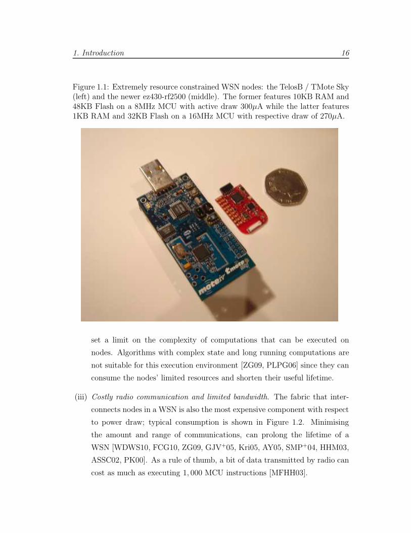
We target the extremely resource constrained end of the Wireless Sensor Network
(WSN) spectrum that comprises nodes such as those shown in Figure 1.1. The
constraining factors that differentiate such nodes from other distributed systems
are:
(i) Limited power resources. Typically, nodes are powered by batteries which
limit their useful lifetime and specify an energy budget that, in most ap-
plications, must be extended as much as possible. Radio communication,
sensing and processing share this budget and pose a challenge to developers
who must serve the application’s purpose and, at the same time, maximise
node lifetime.
(ii) Restricted functionality. Embedded microcontrollers (MCUs), limited RAM
and — in the vast majority of cases — lack of Floating Point Units (FPUs)
1. Introduction 16
Figure 1.1: Extremely resource constrained WSN nodes: the TelosB / TMote Sky(left) and the newer ez430-rf2500 (middle). The former features 10KB RAM and48KB Flash on a 8MHz MCU with active draw 300µA while the latter features1KB RAM and 32KB Flash on a 16MHz MCU with respective draw of 270µA.
set a limit on the complexity of computations that can be executed on
nodes. Algorithms with complex state and long running computations are
not suitable for this execution environment [ZG09, PLPG06] since they can
consume the nodes’ limited resources and shorten their useful lifetime.
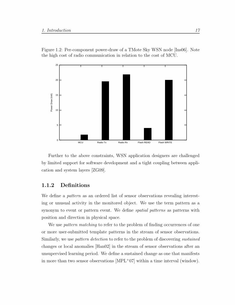
(iii) Costly radio communication and limited bandwidth. The fabric that inter-
connects nodes in a WSN is also the most expensive component with respect
to power draw; typical consumption is shown in Figure 1.2. Minimising
the amount and range of communications, can prolong the lifetime of a
WSN [WDWS10, FCG10, ZG09, GJV+05, Kri05, AY05, SMP+04, HHM03,
ASSC02, PK00]. As a rule of thumb, a bit of data transmitted by radio can
cost as much as executing 1, 000 MCU instructions [MFHH03].
1. Introduction 17
Figure 1.2: Per-component power-draw of a TMote Sky WSN node [Ins06]. Notethe high cost of radio communication in relation to the cost of MCU.
0
5
10
15
20
25
MCU Radio Tx Radio Rx Flash READ Flash WRITE
Pow
er D
raw
(m
A)
Further to the above constraints, WSN application designers are challenged
by limited support for software development and a tight coupling between appli-
cation and system layers [ZG09].
1.1.2 Definitions
We define a pattern as an ordered list of sensor observations revealing interest-
ing or unusual activity in the monitored object. We use the term pattern as a
synonym to event or pattern event. We define spatial patterns as patterns with
position and direction in physical space.
We use pattern matching to refer to the problem of finding occurrences of one
or more user-submitted template patterns in the stream of sensor observations.
Similarly, we use pattern detection to refer to the problem of discovering sustained
changes or local anomalies [Han02] in the stream of sensor observations after an
unsupervised learning period. We define a sustained change as one that manifests
in more than two sensor observations [MPL+07] within a time interval (window).

1. Introduction 18
1.2 Research Methodology
We propose pattern matching and detection algorithms and conduct experimental
evaluation to assess their accuracy and operational profile. Evaluation through
deployment demonstrates suitability of our algorithms for the target platform.
Evaluation through simulation investigates the performance of the proposed al-
gorithms under varying parameters and compares their pattern matching and
detection accuracy against competitive techniques.
The following sections state the goals of this thesis and discuss methods em-
ployed in addressing the research questions.
1.2.1 Requirements and Research Questions
We identify the following requirements for a solution that addresses the problem
of in-network pattern matching and detection:
(i) It should cater for a variety of usage scenarios such as matching user submit-
ted template patterns and also detecting unusual patterns without relying
on prior user information.
(ii) It should reduce network communication for pattern matching and detec-
tion, and only engage in localised communication when required.
(iii) It should execute efficiently on extremely resource constrained WSN nodes.
(iv) It should be compatible with existing WSN paradigms and not require
change of underlying communication protocols to accommodate pattern
matching and detection functionality.
(v) It should accommodate WSN applications with different sampling frequency
requirements performing pattern matching and detection in a timely man-
ner, as close to real time as possible.
The thesis addresses the following questions:
1. Introduction 19
(R1.) Is there a class of algorithms that make in-network pattern matching and
detection feasible for extremely resource constrained nodes?
(R2.) How is the algorithms’ matching/detection performance affected by differ-
ent choice of algorithm parameters?
(R3.) Is this class of algorithms a viable alternative in comparison to other event
detection methods?
(R4.) Are the requirements, as stated above, satisfied by such pattern matching
and detection algorithms?
Question R1 is addressed with the algorithms of Chapter 3 and answered
through deployment in Section 5.1. Question R2 is answered initially through
emulation (Section 4.2) and findings are validated through deployment (Sec-
tion 5.2.1). Question R3 is answered through emulating sensor node streaming
data acquisition in software, and specifically by comparing the temporal domain
pattern detection algorithm against two competitive techniques (Section 4.3.1).
Lastly, R4 is answered with the algorithms of Chapters 3 and 6 which are evalu-
ated with a combination of deployment and simulation.
1.2.2 Research Methods
After reviewing literature related to the problem of pattern matching and detec-
tion, evaluation of the proposed solution was conducted through implementation
and deployment on WSN nodes to assess suitability for the extremely resource
constrained execution environment and compatibility with existing WSN com-
munication protocols.
Simulation experiments were conducted to evaluate the performance of the
algorithms with respect to the rate of true and false positives in the temporal
domain, and pattern event location estimation accuracy in the spatial domain.
Data and tools used in evaluation of the proposed algorithms are widely avail-
able, and our experimental setup is described — Sections 4.1, 5.1 and 7.1 — to
encourage peer review of our findings from the WSN community. The software
1. Introduction 20
developed in this thesis is used by fellow researchers and is publicly available
together with data collected from our deployments to encourage reproducibility
of experiments.
1.3 Contributions
The work described in this thesis makes contributions that address the WSN
application issue of pattern matching and detection, and offers a computation-
ally efficient implementation of reactive functionality. Moreover, it limits radio
communication and MCU active time in order to complement the generic goal of
prolonged WSN lifetime. Specifically, we make the following contributions:
(i) Develop temporal domain in-network pattern matching and detection al-
gorithms that reduce network communication. Described in Chapter 3,
the algorithms cater for exact, approximate, multiple, non-parametric and
probabilistic pattern matching and detection.
(ii) Provide evidence that the proposed algorithms produce consistently good
results in three case studies (Chapter 4) with respect to matching/detection
accuracy. The case studies evaluate different aspects of the algorithms such
as the impact of different parameters to false positives and accuracy in
comparison with other event detection techniques.
(iii) Demonstrate that the algorithms are suitable for extremely resource con-
strained nodes by integer arithmetic refactoring and deployment (Chapter
5). Suitability is further demonstrated by incorporating dynamic sampling
frequency adjustments to reduce MCU active time, and integrate the pro-
posed algorithms with a Publish/Subscribe (Pub/Sub) interface that em-
ploys standard TinyOS communication protocols.
(iv) Introduce an iterative algorithm, based on a geometric computation and
a Kalman filter (Chapter 6), that engages in localised communication to

1. Introduction 21
estimate the location of a spatial event inside the network in a collaborative
manner.
(v) Evaluate the estimation performance of the spatial algorithm and, in par-
ticular, investigate the impact of WSN topology and node placement to the
estimation performance in comparison with a competitive approach (Chap-
ter 7).
We believe that the above contributions provide a competitive pattern match-
ing and detection family of algorithms that can be used in a variety of reactive
WSN applications.
1.4 Assumptions and Limitations
The work proposed in this thesis makes the following assumptions:
• Homogeneous network comprised of extremely resource constrained nodes
with characteristics outlined in Section 1.1.1.
• For location estimation, the single pollutant source and WSN nodes are
stationary. The nodes are aware of their location coordinates which are
accurate and error-free.
The first assumption means that the proposed algorithms are not dependent on
a base station, high capability nodes or centralised coordination.
We recognise the following limitations with respect to the proposed algo-
rithms:
• They do not cater for cross correlated matching and detection of patterns
in multiple dimensions (sensed modalities).
• They operate on windowed observations and are not designed to detect
outliers or single data point events.
• They do not provide historic pattern matching and detection for past events
since nodes, by default, do not store sensor observations.
1. Introduction 22
• They do not take into account dynamic metadata that can change the
interpretation of observations and consequently the outcome of matching
and detection.
• The spatial domain algorithm cannot, in its present form, cater for multiple,
mobile sources and dynamic environmental conditions.
A subset of the above limitations is addressed in directions for future work ex-
plored in Section 8.4.
1.5 Outline of the Thesis
Chapter 2 offers a literature review of event detection and pattern classification
methods for WSNs and sensor data. Temporal pattern matching and detec-
tion algorithms are introduced in Chapter 3 and evaluation through emulation
is conducted in Chapter 4. The latter work can be divided in two categories:
investigation of the effect of algorithm parameter selection to pattern matching
and detection and comparison against competitive methods. Chapter 5 describes
the practical work undertaken for the evaluation of the temporal domain algo-
rithms through full implementation and deployment. Specifically, it presents
the refactoring of our algorithms and associated timing measurements obtained
from WSN nodes that demonstrate suitability for extremely resource constrained
nodes. Furthermore, it presents the dynamic sampling frequency extension to
non-parametric pattern detection, and discusses field validation through a data
centre deployment. Chapter 6 introduces the spatial domain algorithm that tar-
gets location estimation of a pollutant-emitting source and Chapter 7 presents
related findings obtained from simulation experiments that include a comparison
to a competitive maximum selection algorithm. Finally, the thesis concludes in
Chapter 8 with a critical appraisal and a detailed plan for future work.
Chapter 2
Pattern Matching and Detection
in WSNs and Sensor Data
Pattern matching and detection can be addressed with a variety of techniques
such as clustering, density estimation, probabilistic matching, Kalman filtering,
expert systems and string matching. In this chapter, we review techniques that
target WSNs or sensor data and present approaches categorised per application
domain.
Techniques for event detection in environmental monitoring applications are
reviewed in Section 2.1, and Section 2.2 presents approaches for data centre and
structural health monitoring. Section 2.3 reviews pattern matching and detection
in body sensor networks and context aware computing. Network monitoring
and security applications are reviewed in Section 2.4. Approaches for pattern
matching and detection in spacecraft image and telemetry data are discussed
in Section 2.5. Spatial pattern location estimation approaches are reviewed in
Section 2.6 and generic approaches are presented in Section 2.7. Finally, we
summarise our findings in Section 2.8.
23
2. Pattern Matching and Detection in WSNs and Sensor Data 24
2.1 Environmental Monitoring
Lance [WADHW08] addresses resource prioritisation and bandwidth allocation
in WSNs. It is a volcano monitoring application where an unusual pattern is
a signal segment denoting activity that may lead to an eruption. Lance caters
for correlated pattern event detection and it employs an Exponentially Weighted
Moving Average (EWMA) method to detect patterns that trigger data upload to
a base station. In Section 4.3, we conduct a comparison between the proposed
Non-Parametric Pattern Detection algorithm and EWMA with data from the
deployment of Lance.
The approach described in [BRR08] presents a model-based system that aims
to detect and predict river flood pattern events in developing countries. The
suggested model is based on statistical methods such as linear regression. This
approach assumes a tiered architecture where resource-constrained sensor nodes
transmit summaries and statistics of raw observations to a set of high capability
computation nodes. The latter determine data correctness, feed it to the model
for event detection/prediction and possibly request additional data from sensors
to reduce uncertainty. PRESTO [DGL+05] is another tiered system based on
an ARIMA (Auto Regressive Integrated Moving Average) forecasting model that
detects unusual patterns by comparing predicted values to sensor observations.
The work described in [KSW+08] employs the symbolic conversion algorithm
SAX [LKLC03], also used by temporal domain algorithms proposed in this thesis,
to obtain a discretised version of Electrical Penetration Graph (EPG) data relat-
ing to the behaviour of insects. Specifically, the authors developed a constant-time
version of the Time Series Bitmap (TSB) [KLK+05] algorithm that can be used on
constrained devices for real-time EPG classification. Their aim is to improve un-
supervised classification of insects’ lifecycle data in experimental conditions. The
work does not provide implementation details but a deployment is mentioned in
their future plans.
The approach described in [BHL07] presents a distributed algorithm for de-
tecting ecological anomalies as well as estimating erroneous or missing data. The
2. Pattern Matching and Detection in WSNs and Sensor Data 25
proposed method performs automatic inference and prediction based on statisti-
cal distributions of differences in observations between a node and its neighbours.
Nodes compute the distribution of differences to perform a p-test that determines
the likelihood of an observation exceeding a significance level. One drawback of
this approach is the radio communication overhead required to compute the dis-
tribution of spatial differences.
2.2 Data Centre and Structural Monitoring
Research described in [PMSR09] proposes a temporal data mining solution to
optimise the performance of data centre chillers. Sensor nodes deployed in data
centres observe temperature and humidity data that varies according to the load
of individual servers, storage and networking equipment. This system illustrates
the operation a Wireless Sensor Actuator Network (WSAN): depending on ob-
served patterns, a decision must be made to turn on/off chillers, select a utili-
sation range and react to cooling demands. The authors focus on motif mining,
which is the identification of frequently occurring temporal patterns. First, a
string representation of the sensor observations is generated with the symbolic
aggregate approximation (SAX) [LKLC03] algorithm. A Run-Length Encoding
(RLE) of the symbolic sequence records transitions from one symbol to another.
Frequent episode mining is conducted over the sequence of transitions to identify
the underlying efficiency profile of the data centre under different environmental
circumstances.
The work described in [XLCL06] employs contour map matching to determine
whether a user-supplied pattern matches sensor produced observations. The ap-
plication scenario is event detection in coal mines, monitoring gas, dust and water
leakage events as well as high/low oxygen density regions. A limitation is that
it assumes users capable of describing the pattern of interest as distributions of
an attribute over space and variations of this distribution over time. A related
approach [LLC07], targeting gas leakage events in mines, tasks nodes to construct
3-dimensional gradient data maps which are transmitted to a sink and compared
2. Pattern Matching and Detection in WSNs and Sensor Data 26
to predefined patterns.
Wisden [XRC+04] is a system that employs a wavelet integer lifting transform
to detect patterns in structural health monitoring applications. It uses wavelet
compression to store vibration data locally and transmits a lossy version to the
base station. Its pattern detection component operates as follows: if samples
within a window are comparable in value and of low magnitude then the structure
is perceived to be in a quiescent state. Such windows are considered normal
and compressed using RLE, in contrast to pattern events which are transmitted
uncompressed. One strength of this approach is that the computational efficiency
of the event detection mechanism is verified through deployment.
The system presented in [LKQ+03], aims to detect patterns in order to di-
agnose potential damages that could affect the integrity of filament wound com-
posite structures such as solid rocket motors and liquid fuel containers. It uses
actuator nodes either embedded in the structure or placed on its surface, to emit
a diagnostic stress wave signal. A neighbouring sensor node captures the signal
and compares it to a baseline normal signal. If a difference is observed, it indi-
cates change in the surface of the structure that can be attributed to damage.
One challenge with this described method is difficulty of generalisation — for
instance, stress layers’ placement had a significant impact to detection accuracy
— although there is mention of expanding the work such that it applies on other
structures and different materials.
2.3 Body Sensor Networks and Context Aware
Systems
The approach described in [HJCX08] introduces wavelet-based ECG data mining
for Body Sensor Networks (BSNs). The system targets remote patient monitor-
ing through a combination of resource constrained nodes and offline processing.
Nodes are responsible for ECG noise filtering and periodic transmission of ECG
2. Pattern Matching and Detection in WSNs and Sensor Data 27
waveforms to a central server for processing. The server employs feature extrac-
tion with wavelet transforms and the Local Holder Exponent (LHE) function.
Support Vector Machines (SVMs) are used for classification of ECG signal frag-
ments. In contrast to our methods that process data inside the network, this
approach incurs the communication cost of transmitting observations to a base
station.
BiosensorNET [KHW+07] is a BSN comprising resource constrained nodes
for near real-time heart rate variability analysis of ECG signals. It is based on
two algorithmic layers: a real-time layer extracts the QRS complex which is the
significant part of the ECG signal. It passes the QRS to a near real-time layer
that performs variability analysis on the frequency domain and invokes further
processing only if it determines that the QRS is significant. To our knowledge, this
is one of the first efforts to address both pattern detection and implementation
for extremely resource constrained nodes in the field of BSNs.
The work described in [SRT07] employs the symbolic aggregate approxima-
tion SAX [LKLC03] algorithm for string conversion of gesture data obtained
by accelerometers and gyroscopes worn by human subjects. Gestures are char-
acterised by the movement of limbs in Cartesian space and their identification
and classification through wearable sensors can assist in determining the context
and activity of persons. The proposed approach, similar to our work, offers ap-
proximate pattern matching with a different distance metric, the edit distance.
Although they target real-time gesture classification in constrained sensor nodes,
the work lacks WSN deployment evidence and performance results are collected
in a desktop-class machine. A related system [WYC+06] targets human activity
recognition from sensor accelerometer observations using decision trees, neural
networks and Support Vector Machines (SVMs).
A method aimed at pattern matching over trajectory data is described in
[BCFL09] where authors propose a distance metric to determine similarity be-
tween trajectory subsequences. Recognising patterns in trajectory data has appli-
cations ranging from remote monitoring of elderly patients to military detection
of enemy movements. Pattern detection is performed by testing whether a time
2. Pattern Matching and Detection in WSNs and Sensor Data 28
window has fewer than a predetermined number of neighbours in its left and right
sliding windows. Experimental results show efficiency with respect to processing
time measurements, however evaluation is conducted offline lacking validation on
WSN nodes.
The approach of [HMBE06] targets context-aware computing and specifically
mining for unusual patterns in observations representing human interactions with
their environment. The authors propose the use of a Suffix Tree data structure
to encode the structural information of activities and their event statistics at dif-
ferent temporal resolutions. The method aims to identify unusual patterns that
either consist of structural differences to normal behaviour or differences based
on the frequency of occurrence of motifs. The approach relies on training data
to construct the dictionary of legitimate behaviour and sequences are classified
as unusual using a match statistic computed over the suffix tree. The strength of
the approach is that suffix tree traversal requires linear time, however dynamic
suffix tree construction and update is not always suitable to platforms with se-
vere resource constraints due to dynamic memory allocation demands of such
operations.
2.4 Network Monitoring and Security
The approach described in [WDWS10] presents a system for distributed pattern
event detection using training data or statistical means. The system is based
on feature extraction by discretisation in time intervals and computation of the
difference between minimal and maximal observations for each interval. The
output is a feature vector that is compared in terms of Euclidean distance against
a number of prototype vectors. One strength of this approach is that is has been
evaluated through a deployment in a security application detecting trespassing at
a construction site. However, unlike our approach, training requires considerable
memory and processing resources and is performed on a desktop-class machine
rather than on WSN nodes.
The work described in [DSS07] introduces Artificial Immune Systems (AIS)
2. Pattern Matching and Detection in WSNs and Sensor Data 29
for misbehaviour detection. AIS are inspired from the human immune system and
its ability to detect harmful agents such as viruses and infections. The method
facilitates local learning and detection with a gene-based approach. Each node
maintains a local set of detectors produced by negative selection from a larger set
of randomly generated detectors tested on a set of self strings. The detectors test
new strings that represent local network behaviour, and detect non-self strings
denoting unusual patterns. The approach has been evaluated using MAC layer
messages and targets detection of local patterns that indicate misbehaviour over
a layer of the OSI reference model stack.
The approach described in [HGH+06], proposes a Principal Component Anal-
ysis (PCA) method for detecting unusual patterns with complex thresholds in
a distributed manner. Nodes transmit observations to a coordinator responsible
for firing a trigger based on the aggregate behaviour of a subset of nodes. The
individual nodes perform filtering such that they transmit only when observations
deviate significantly from the last transmitted data. Detection is accomplished
with two window triggers that fire on persistent threshold violations over a fixed
or varying window of observations. Although the approach is aimed at detecting
unusual network traffic patterns, it can generalise to other WSN applications.
The main criticism is that coordinator nodes introduce single points of failure in
the detection scheme.
A related approach [LNLP06], considers intrusion detection in WSNs from
samples of routing traffic. First, feature selection of traffic and non-traffic related
data is performed in order to learn the distribution of values affecting routing
conditions and traffic flows. Second, pattern detection is performed locally by
comparing a window of observations to previously collected normal data. This
window contains samples mapped to points in a feature space and are analysed
together with their surrounding region. If a point lies in a sparse region of space
is classified as unusual using a fixed-width clustering algorithm. The method is
capable of locally detecting novel patterns, but it is limited by the number of
modelled attacks.
2. Pattern Matching and Detection in WSNs and Sensor Data 30
2.5 Spacecraft and Telemetry Pattern Classifi-
cation
In [CWC+07], the authors describe mining scientific data on-board a spacecraft in
order to react to dynamic patterns of interest as well as to provide data summaries
and prioritisation. Three image pattern recognition algorithms are presented that
were employed on board the Mars Odyssey spacecraft to detect polar cap edges
and atmospheric opacity events.
The approach described in [SOM07] presents three unsupervised pattern recog-
nition algorithms evaluated offline using historical data obtained from a space
shuttle main engine, comprising up to 90 sensors, for the objective of future in-
clusion in the Ares I and Ares V launch systems. The algorithms employ Support
Vector Machines (SVMs), clustering and nearest neighbour for pattern classifica-
tion.
A system aimed at automatic satellite reliability monitoring is described in
[DTP91]. The diagnosis of faults from, sometimes limited, sensor data is per-
formed by an expert system. The authors describe how the expert system was
built even with limited knowledge and its ability to perform inexact reasoning to
accommodate sparse sensors. A disadvantage is inherited from expert systems
and is attributed to the supervised learning required to describe possible fault
states.
2.6 Spatial Pattern Location Estimation
The approach described in [CYR+08] addresses an instance of the spatial loca-
tion estimation problem considered in Chapter 6. The authors address spatial
pattern location estimation of a radioactive source using an iterative pruning
data fusion algorithm tolerant of measurement noise. The system is based on the
ratio-of-square-distance (RoSD) location estimation algorithm that uses observa-
tions from three nodes and improves estimation accuracy as more nodes become
2. Pattern Matching and Detection in WSNs and Sensor Data 31
available. The outcome of RoSD algorithm is fed into an iterative pruning clus-
tering algorithm that provides a geometric solution to the location estimation
problem. Two strengths of this approach is the evaluation of realistic noise and
error conditions, and the implementation on WSN nodes.
The work described in [GJV+05] proposes VigilNet, a hierarchical system for
in-network detection and classification of vehicles and persons. Using a combina-
tion of magnetometers, motion sensors, and microphones, lower tier nodes apply
a moving average aggregation scheme and forward their summaries to dynamic
cluster heads. The cluster heads examine spatio-temporal correlations, compute
confidence scores over the aggregate data and forward the outcome to a base
station. The base station finalises classification results with linear regression
and estimates metadata such as target location and velocity. One strength of
this system is that it validates spatial pattern detection through deployment on
extremely resource constrained nodes.
The distributed Kalman filter proposed in [SOSM05] targets location estima-
tion in WSNs with imperfect communication links based on an iterative spatial
averaging algorithm. It introduces a transfer function that describes the error
behaviour of the distributed Kalman filter in the case of stationary noise pro-
cesses. The authors focus on location estimation of sonic sources using acoustic
sensors and claim that their method generalises to other domains. Evaluation
is conducted through simulation and the description lacks WSN implementation
details.
We adopt the gas distribution and sensor response model of Ishida [INM97],
described in Section 7.1. In this work, the authors deploy a mobile robot that
detects the concentration of gas in the atmosphere and moves to appropriate
locations in an attempt to estimate the source location. Achieved through fitting
the gas distribution model to the sensor response at each location, they provide
a sensing algorithm that is also capable of estimating the release rate of the gas
pollutant.
Generic coarse grained location estimation techniques include the Centroid
Calculation or Point-in-Triangle (PIT) methods [Kri05]. A variation of the former
2. Pattern Matching and Detection in WSNs and Sensor Data 32
is employed in the geometric computation described in Section 6.3 and used by
our spatial location estimation algorithm. A refinement of the PIT technique is
the Approximate Point in Triangle (APIT) described in [HHB+03]. A geometric
approach based on the circles of Apollonius is described in [CP07]. A family
of methods based on Time Difference of Arrival (TDOA) with geometric and
numerical solutions, can be found in [MPR03], [Rao06], and [XRS07].
2.7 Generic Approaches and Additional Appli-
cations
In [RBLP09] the authors propose a pattern detection system based on elliptical
anomalies which are defined by the ellipsoid or hyperellipsoid caused by the region
of distance around the mean of two or more monitored variables. Given a set of
column vectors representing sensor observations, the aim is to partition the set
into normal and unusual observations. The algorithms for first and second order
elliptical anomaly detection can be fully distributed in the network. A drawback
is that computational cost on WSN nodes is not evaluated, although the authors
assume resource constrained nodes.
The approach presented in [SWJR07] targets the problem of pattern detection
using a density test for distributional changes. Possibly multidimensional sensor
observations are tested against a baseline data set with a statistical test that
determines whether data points in the set of observations were sampled from the
same underlying distribution that produced the baseline set. The test statistic
is distribution-free and based on kernel density estimation and Gaussian kernels.
The baseline distribution is inferred using a combination of the kernel density
estimator with an Expectation Maximisation (EM) algorithm. The capability
of recognising patterns occurring at multiple data dimensions simultaneously is
a strength of this approach. However it lacks implementation details for WSN
nodes and is only evaluated through simulation.
2. Pattern Matching and Detection in WSNs and Sensor Data 33
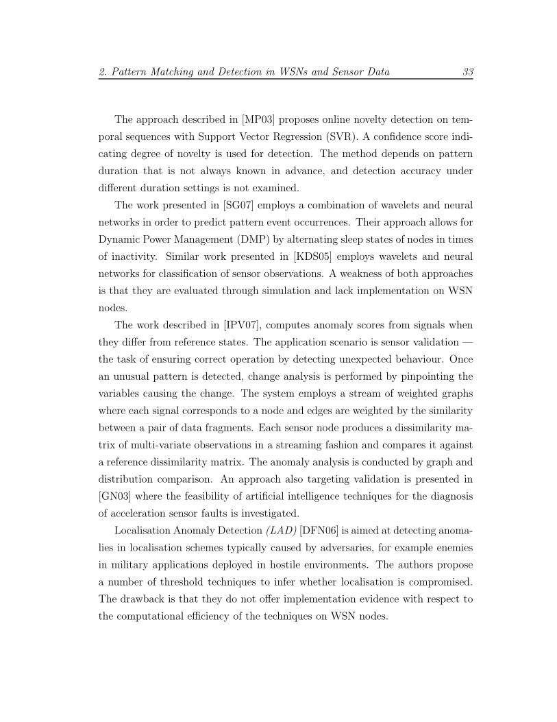
The approach described in [MP03] proposes online novelty detection on tem-
poral sequences with Support Vector Regression (SVR). A confidence score indi-
cating degree of novelty is used for detection. The method depends on pattern
duration that is not always known in advance, and detection accuracy under
different duration settings is not examined.
The work presented in [SG07] employs a combination of wavelets and neural
networks in order to predict pattern event occurrences. Their approach allows for
Dynamic Power Management (DMP) by alternating sleep states of nodes in times
of inactivity. Similar work presented in [KDS05] employs wavelets and neural
networks for classification of sensor observations. A weakness of both approaches
is that they are evaluated through simulation and lack implementation on WSN
nodes.
The work described in [IPV07], computes anomaly scores from signals when
they differ from reference states. The application scenario is sensor validation —
the task of ensuring correct operation by detecting unexpected behaviour. Once
an unusual pattern is detected, change analysis is performed by pinpointing the
variables causing the change. The system employs a stream of weighted graphs
where each signal corresponds to a node and edges are weighted by the similarity
between a pair of data fragments. Each sensor node produces a dissimilarity ma-
trix of multi-variate observations in a streaming fashion and compares it against
a reference dissimilarity matrix. The anomaly analysis is conducted by graph and
distribution comparison. An approach also targeting validation is presented in
[GN03] where the feasibility of artificial intelligence techniques for the diagnosis
of acceleration sensor faults is investigated.
Localisation Anomaly Detection (LAD) [DFN06] is aimed at detecting anoma-
lies in localisation schemes typically caused by adversaries, for example enemies
in military applications deployed in hostile environments. The authors propose
a number of threshold techniques to infer whether localisation is compromised.
The drawback is that they do not offer implementation evidence with respect to
the computational efficiency of the techniques on WSN nodes.
2. Pattern Matching and Detection in WSNs and Sensor Data 34
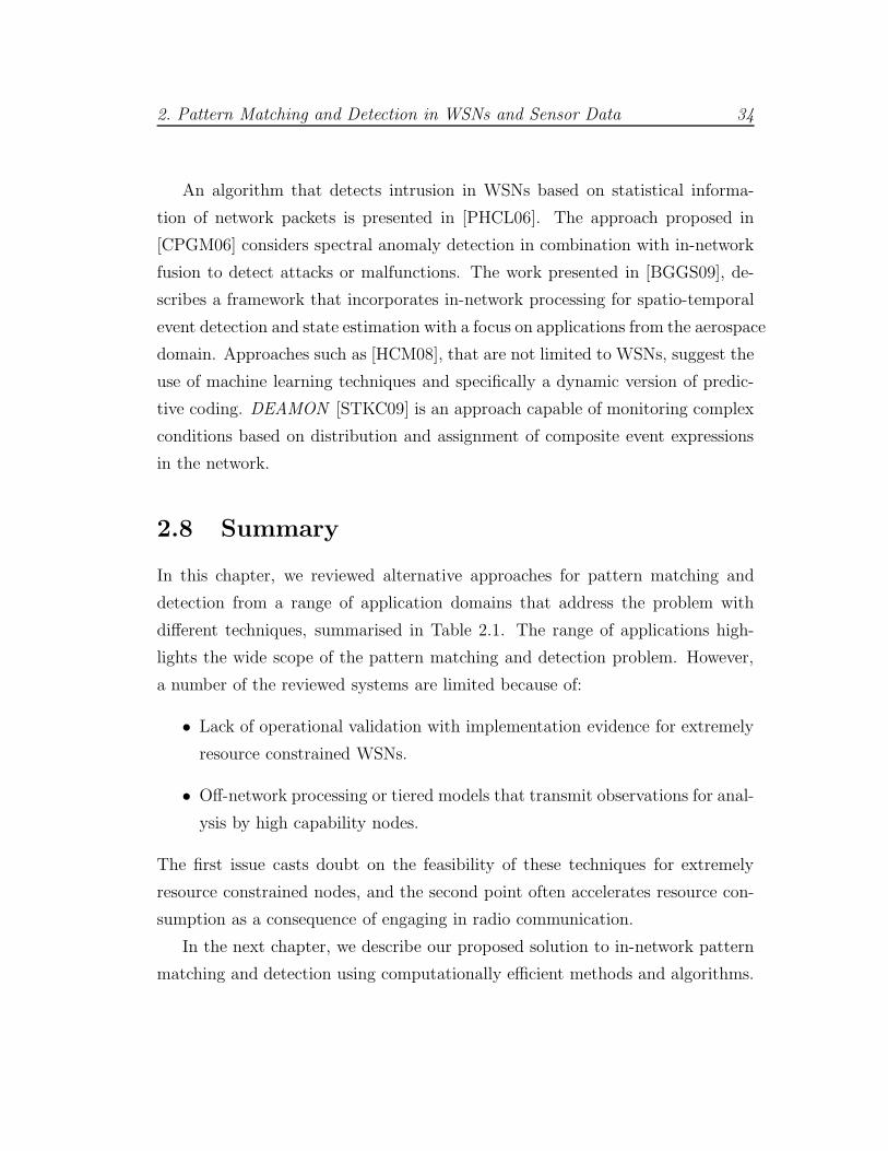
An algorithm that detects intrusion in WSNs based on statistical informa-
tion of network packets is presented in [PHCL06]. The approach proposed in
[CPGM06] considers spectral anomaly detection in combination with in-network
fusion to detect attacks or malfunctions. The work presented in [BGGS09], de-
scribes a framework that incorporates in-network processing for spatio-temporal
event detection and state estimation with a focus on applications from the aerospace
domain. Approaches such as [HCM08], that are not limited to WSNs, suggest the
use of machine learning techniques and specifically a dynamic version of predic-
tive coding. DEAMON [STKC09] is an approach capable of monitoring complex
conditions based on distribution and assignment of composite event expressions
in the network.
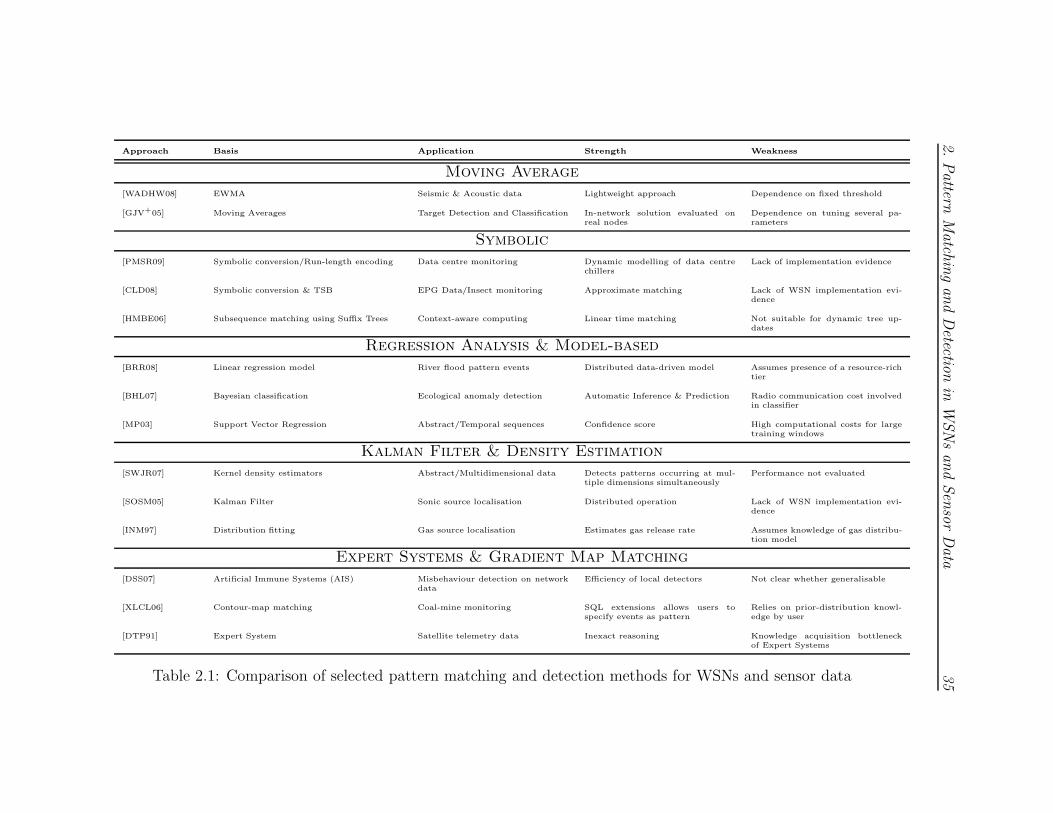
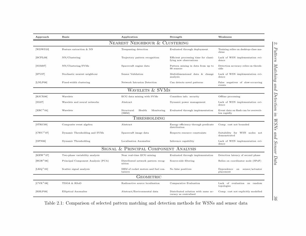
2.8 Summary
In this chapter, we reviewed alternative approaches for pattern matching and
detection from a range of application domains that address the problem with
different techniques, summarised in Table 2.1. The range of applications high-
lights the wide scope of the pattern matching and detection problem. However,
a number of the reviewed systems are limited because of:
• Lack of operational validation with implementation evidence for extremely
resource constrained WSNs.
• Off-network processing or tiered models that transmit observations for anal-
ysis by high capability nodes.
The first issue casts doubt on the feasibility of these techniques for extremely
resource constrained nodes, and the second point often accelerates resource con-
sumption as a consequence of engaging in radio communication.
In the next chapter, we describe our proposed solution to in-network pattern
matching and detection using computationally efficient methods and algorithms.
2.Pattern
Match
ingandDetectio
nin
WSNsandSen
sorData
35
Approach Basis Application Strength Weakness
Moving Average
[WADHW08] EWMA Seismic & Acoustic data Lightweight approach Dependence on fixed threshold
[GJV+05] Moving Averages Target Detection and Classification In-network solution evaluated onreal nodes
Dependence on tuning several pa-rameters
Symbolic
[PMSR09] Symbolic conversion/Run-length encoding Data centre monitoring Dynamic modelling of data centrechillers
Lack of implementation evidence
[CLD08] Symbolic conversion & TSB EPG Data/Insect monitoring Approximate matching Lack of WSN implementation evi-dence
[HMBE06] Subsequence matching using Suffix Trees Context-aware computing Linear time matching Not suitable for dynamic tree up-dates
Regression Analysis & Model-based
[BRR08] Linear regression model River flood pattern events Distributed data-driven model Assumes presence of a resource-richtier
[BHL07] Bayesian classification Ecological anomaly detection Automatic Inference & Prediction Radio communication cost involvedin classifier
[MP03] Support Vector Regression Abstract/Temporal sequences Confidence score High computational costs for largetraining windows
Kalman Filter & Density Estimation
[SWJR07] Kernel density estimators Abstract/Multidimensional data Detects patterns occurring at mul-tiple dimensions simultaneously
Performance not evaluated
[SOSM05] Kalman Filter Sonic source localisation Distributed operation Lack of WSN implementation evi-dence
[INM97] Distribution fitting Gas source localisation Estimates gas release rate Assumes knowledge of gas distribu-tion model
Expert Systems & Gradient Map Matching
[DSS07] Artificial Immune Systems (AIS) Misbehaviour detection on networkdata
Efficiency of local detectors Not clear whether generalisable
[XLCL06] Contour-map matching Coal-mine monitoring SQL extensions allows users tospecify events as pattern
Relies on prior-distribution knowl-edge by user
[DTP91] Expert System Satellite telemetry data Inexact reasoning Knowledge acquisition bottleneckof Expert Systems
Table 2.1: Comparison of selected pattern matching and detection methods for WSNs and sensor data
2.Pattern
Match
ingandDetectio
nin
WSNsandSen
sorData
36
Approach Basis Application Strength Weakness
Nearest Neighbour & Clustering
[WDWS10] Feature extraction & NN Trespassing detection Evaluated through deployment Training relies on desktop-class ma-chine
[BCFL09] NN/Clustering Trajectory pattern recognition Efficient processing time for classi-fying new observations
Lack of WSN implementation evi-dence
[SOM07] NN/Clustering/SVMs Spacecraft engine data Pattern mining in data from up to90 sensors
Detection accuracy relies on thresh-olds
[IPV07] Stochastic nearest neighbour Sensor Validation Multidimensional data & changeanalysis
Lack of WSN implementation evi-dence
[LNLP06] Fixed-width clustering Network Intrusion Detection Can detects novel patterns False negatives of slow-occurringevents
Wavelets & SVMs
[HJCX08] Wavelets ECG data mining with SVMs Considers info. security Offline processing
[SG07] Wavelets and neural networks Abstract Dynamic power management Lack of WSN implementation evi-dence
[XRC+04] Wavelets Structural Health Monitoring(SHM)
Evaluated through implementation Event data on flash can be overwrit-ten rapidly
Thresholding
[STKC09] Composite event algebra Abstract Energy efficiency through predicatedistribution
Comp. cost not bounded
[CWC+07] Dynamic Thresholding and SVMs Spacecraft image data Respects resource constraints Suitability for WSN nodes notdemonstrated
[DFN06] Dynamic Thresholding Localisation Anomalies Inference capability Lack of WSN implementation evi-dence
Signal & Principal Component Analysis
[KHW+07] Two-phase variability analysis Near real-time ECG mining Evaluated through implementation Detection latency of second phase
[HGH+06] Principal Component Analysis (PCA) Distributed network pattern recog-nition
Source-side filtering Relies on coordinator node (SPoF)
[LKQ+03] Scatter signal analysis SHM of rocket motors and fuel con-tainers
No false positives Dependence on sensor/actuatorplacement
Geometric
[CYR+08] TDOA & RSoD Radioactive source localisation Comparative Evaluation Lack of evaluation on randomtopologies
[RBLP09] Elliptical Anomalies Abstract/Environmental data Distributed solution with same ac-curacy as centralised
Comp. cost not explicitly modelled
Table 2.1: Comparison of selected pattern matching and detection methods for WSNs and sensor data
Chapter 3
Pattern Matching and Detection
in the Temporal Domain
This chapter introduces algorithms for in-network pattern matching and detection
in the temporal domain. The algorithms process incoming sequences of streaming
sensor observations, transform them to a symbolic representation and determine
whether the resulting string matches one or more user-submitted template pat-
terns or, in lieu of the latter, classify it as normal or unusual. All the algorithms
presented in this chapter are autonomous by design and do not rely on network
communication for pattern matching and detection.
We first provide an overview of symbolic conversion, in Section 3.1, which
forms the basis for our algorithms. The pattern matching and detection algo-
rithms are presented in Sections 3.2 to 3.5, and a summary of their characteristics
is presented in Section 3.6.
3.1 The Basis for Pattern Matching and Detec-
tion
The algorithms proposed in this chapter employ an in-network transformation
phase where numeric sensor observations are discretised to produce a symbolic
37
3. Pattern Matching and Detection in the Temporal Domain 38
representation. A sliding window is applied to transform numeric observations to
strings with the Symbolic Aggregate Approximation algorithm (SAX) [LKLC03].
Pattern matching and detection is performed in-the-network by operating on the
symbolic representation alone.
Two broad usage scenarios are considered: first, a matching case where a
sensor-produced string (henceforth, sensor string) is compared to one or more
user submitted template patterns (henceforth templates) and, second, a detection
case where templates for comparison are unavailable and nodes must classify
incoming sensor strings following an unsupervised learning phase.
3.1.1 Advantages of Symbolic Transformation
Transforming numeric sensor observations to sequences of symbols offers the fol-
lowing advantages:
• It fixes the computational cost of pattern matching and detection to a
value known at compile-time (explored further in Chapter 5). This type of
operational predictability is desirable in WSNs since it makes application
behaviour deterministic [LGH+05].
• It allows the application of well-known techniques, from the fields of bioin-
formatics, probability theory and data mining, that can be combined to
meet the requirements of pattern matching and detection.
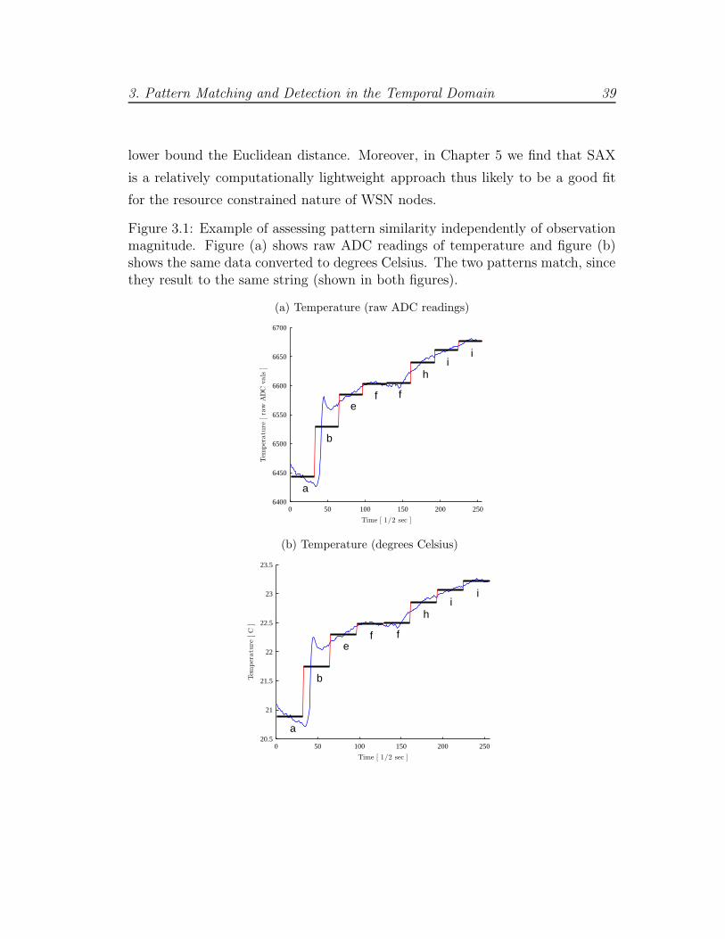
• It allows pattern similarity to be assessed independently of magnitude of
numeric observations, since it converts numeric sequences to strings of a
finite, and typically small (under 15 characters), alphabet. An example of
scale independence is shown in Figure 3.1.
Further to the above advantages, we specifically considered variants of the SAX
algorithm because it has a proven track record in data mining across a number of
related domains ranging from biometric recognition [CMY05] to anticipating the
formation of tornadoes [MRK+07]. It has desirable properties such as dimension-
ality and numerosity reduction as well as a distance metric that is guaranteed to
3. Pattern Matching and Detection in the Temporal Domain 39
lower bound the Euclidean distance. Moreover, in Chapter 5 we find that SAX
is a relatively computationally lightweight approach thus likely to be a good fit
for the resource constrained nature of WSN nodes.
Figure 3.1: Example of assessing pattern similarity independently of observationmagnitude. Figure (a) shows raw ADC readings of temperature and figure (b)shows the same data converted to degrees Celsius. The two patterns match, sincethey result to the same string (shown in both figures).
(a) Temperature (raw ADC readings)
0 50 100 150 200 2506400
6450
6500
6550
6600
6650
6700
Time [ 1/2 sec ]
Tem
per
atu
re[ra
wA
DC
vals
]
a
b
ef f
hi
i
(b) Temperature (degrees Celsius)
0 50 100 150 200 25020.5
21
21.5
22
22.5
23
23.5
Time [ 1/2 sec ]
Tem
per
atu
re[C
]
a
b
ef f
hi
i
3. Pattern Matching and Detection in the Temporal Domain 40
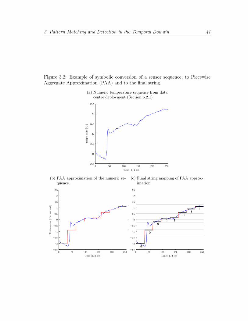
3.1.2 An Overview of Symbolic Aggregate Approximation
The proposed algorithms treat SAX as a black box that takes a numeric sensor
sequence of observations as input and returns a reduced string representation as
output. Symbolic conversion takes place in three phases:
(i) Normalise the sequence u of numeric sensor observations to a centred, scaled
version where the i element is given by:
ui − µ
σ, (3.1)
where µ is the mean of u and σ is the standard deviation.
(ii) Transform the normalised sequence to a Piecewise Aggregate Approxima-
tion (PAA) representation. PAA reduces the length of the sequence using
piecewise polynomial approximation which is compression with a numeros-
ity reduction technique that divides the sequence into w equal-sized frames.
The mean value of data falling within a frame is computed and a vector of
these values comprises the data-reduced PAA representation.
(iii) The final step of the conversion process is a table lookup operation. The
lookup table is a two-dimensional tiling of a sorted list of numbers B =
β1, β2, . . . , βα−1 such that the area under a N(0, 1) Gaussian curve from βi
to βi+1 is equal to 1αwhere α is the size of the alphabet Σ. It is assumed
that β0 and βα are −∞ and +∞ respectively. A sample table for a 10-letter
alphabet is shown in Table 3.1.
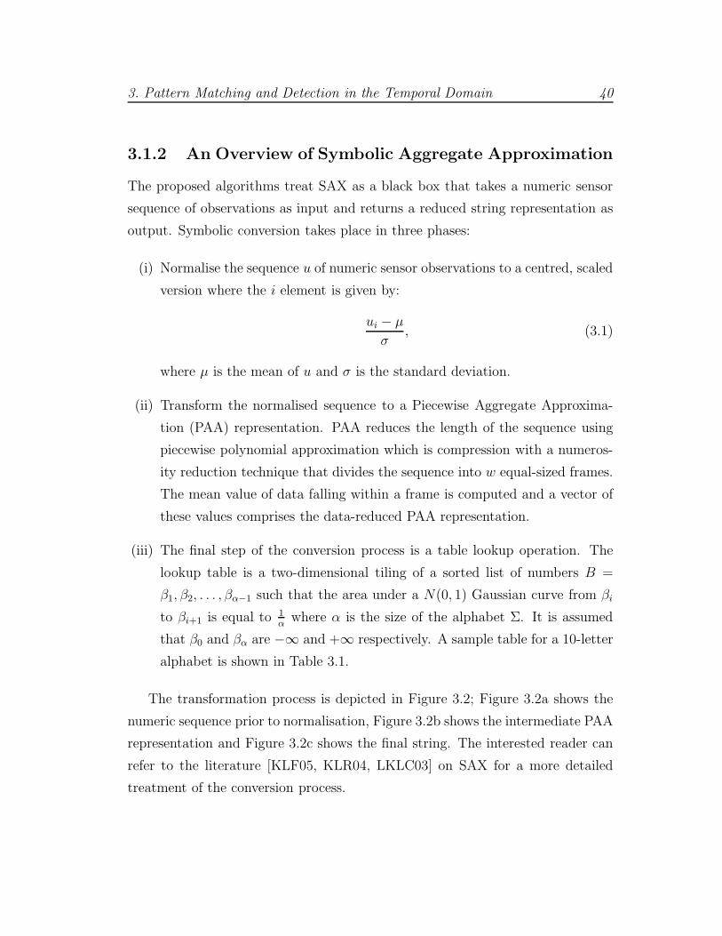
The transformation process is depicted in Figure 3.2; Figure 3.2a shows the
numeric sequence prior to normalisation, Figure 3.2b shows the intermediate PAA
representation and Figure 3.2c shows the final string. The interested reader can
refer to the literature [KLF05, KLR04, LKLC03] on SAX for a more detailed
treatment of the conversion process.
3. Pattern Matching and Detection in the Temporal Domain 41
Figure 3.2: Example of symbolic conversion of a sensor sequence, to PiecewiseAggregate Approximation (PAA) and to the final string.
(a) Numeric temperature sequence from datacentre deployment (Section 5.2.1)
0 50 100 150 200 25020.5
21
21.5
22
22.5
23
23.5
Time [ 1/2 sec ]
Tem
per
atu
re[C
]
(b) PAA approximation of the numeric se-quence.
0 50 100 150 200 250−2.5
−2
−1.5
−1
−0.5
0
0.5
1
1.5
2
2.5
Time [1/2 sec]
Tem
per
atu
re[N
orm
alise
d]
(c) Final string mapping of PAA approx-imation.
0 50 100 150 200 250−2.5
−2
−1.5
−1
−0.5
0
0.5
1
1.5
2
2.5
a
b
ef f
hi
i
Time [ 1/2 sec ]
Tem
per
atu
re[N
orm
alise
d]

3. Pattern Matching and Detection in the Temporal Domain 42
3.1.3 Assessing Pattern Similarity and Probability
With the exception of the probabilistic detection and multiple matching algo-
rithms (Sections 3.3 and 3.5), we employ a distance function to quantify the
difference between two string representations u and r. Assuming u is the sensor
string and r is the template, the calculation depends on a lookup table (Table
3.1) and the below equation:
‖u− r‖S =
√
|u||u|
√
√
√
√
|u|∑
i=1
(dist(ui, ri))2, (3.2)
where |u| denotes the length of the input window representing the length of the
numeric sensor sequence, |u| denotes the length of its corresponding string repre-
sentation, and dist(ui, ri) denotes a lookup to the table (Table 3.1) for characters
i of strings u and r, for instance dist(a, c) = 0.1936.
The two mutually exclusive labels assigned in classification of incoming strings
with the matching algorithms are interesting and normal. Similarly, the pattern
detection algorithms classify a sensor string as either unusual or normal. The
matching and detection outcomes depend on which of the proposed algorithms is
chosen, and are obtained in the following manner:
(i) In the case of matching, a sensor string u is accepted as a pattern event
and classified as interesting if ‖u− r‖S = 0 (exact match) or ‖u− r‖S ≤ θ
(approximate match) or u is a substring of r (multiple match), where θ
stands for a user-supplied distance threshold.
(ii) In the case of inverted matching, a sensor string is rejected (not pattern
a b c d e f g h i k
a 0 0 0.1936 0.5776 1.0609 1.6384 2.3409 3.24 4.4944 6.5536b 0 0 0 0.1024 0.3481 0.7056 1.1881 1.8496 2.8224 4.4944c 0.1936 0 0 0 0.0729 0.2704 0.5929 1.0816 1.8496 3.24d 0.5776 0.1024 0 0 0 0.0625 0.25 0.5929 1.1881 2.3409e 1.0609 0.3481 0.0729 0 0 0 0.0625 0.2704 0.7056 1.6384f 1.6384 0.7056 0.2704 0.0625 0 0 0 0.0729 0.3481 1.0609g 2.3409 1.1881 0.5929 0.25 0.0625 0 0 0 0.1024 0.5776h 3.24 1.8496 1.0816 0.5929 0.2704 0.0729 0 0 0 0.1936i 4.4944 2.8224 1.8496 1.1881 0.7056 0.3481 0.1024 0 0 0k 6.5536 4.4944 3.24 2.3409 1.6384 1.0609 0.5776 0.1936 0 0
Table 3.1: Sample Distance Lookup Table for a 10-letter Alphabet.
3. Pattern Matching and Detection in the Temporal Domain 43
event) and classified as normal if ‖u − r‖S 6= 0 (inverted exact match)
or ‖u − r‖S > θ (inverted approximate match) or u is not a substring
of r (inverted multiple match). For inverted detection, the most recent
sensor string ut is rejected (not pattern event) and classified as normal if
‖ut−ut−1‖S ≤ θ (inverted non-parametric detection) or P (ut) 6= 0 (inverted
probabilistic detection), where ut is the string obtained at time t (similar
for t− 1), θ is obtained as a maximum learnt distance between temporally
adjacent strings, and P (ut) is the path probability of string ut.
(iii) In the case of detection, the most recent sensor string ut is accepted as a
pattern event and classified as unusual if ‖ut− ut−1‖S > θ (non-parametric
detection) or P (ut) = 0 (probabilistic detection).
In summary, a sensor string is classified as interesting if it matches a template
exactly or approximately, otherwise it is classified as normal. Multiple pattern
matching assumes |r| ≫ |u|, where |r| is the cumulative length of the templates
(henceforth, the text) and |u| is the length of the sensor string. In this case,
classification reduces to an exact string matching problem that classifies the string
as interesting, if u is a substring of r. Non-parametric pattern detection compares
temporally adjacent sensor strings and classifies the most recent as unusual if it
exceeds a maximum distance learnt during a training phase. Probabilistic pattern
detection computes the path probability of P (ut), given some learning data, and
classifies a sensor string as normal if it has a non-zero probability of occurrence,
or otherwise unusual.
3.2 Exact and Approximate Pattern Matching
Exact and approximate pattern matching assumes that users are able to de-
scribe patterns of interest. An example is a user with observations from past or
related deployments, submitting one or more ordered subsets of observations as
templates. A WSN node receives a template, stores it and attempts matching
against incoming sensor strings. However, due to node storage access costs and

3. Pattern Matching and Detection in the Temporal Domain 44
Algorithm 3.1 Exact Pattern Matching (EPM) Algorithm
Require: template 6= ε1: if template is numeric then2: r ← int sax(template)3: else4: r ← template
5: end if6: repeat7: ur ← int sax(sensor-values[])8: δ ← ‖ut − r‖S9: until δ == 010: call Notify and goto line 6
limitations, historic searches are not supported — a node cannot match a user-
submitted template against past sensor strings as the nodes do not, by default,
store past strings. Instead, they apply a sliding window over the stream of obser-
vations, convert them to a string and attempt to match against user-submitted
templates, close to real-time.
Matching, shown in lines 8-9 of Algorithms 3.1 and 3.2, is performed as a
distance calculation between two strings: the user-submitted template and the
sensor string. The distance is calculated using a character look up table and the
SAX distance metric, both discussed in Section 3.1.3. Matching is not tightly-
coupled with the specific distance metric and alternative metrics are possible.
The approximate matching algorithm is a variation on exact pattern matching.
In order to determine whether the sensor string matches a template, the output
of the distance calculation ‖u − r‖S is compared to a threshold θ (line 9 of the
algorithms) as described previously (Section 3.1.3). The threshold value depends
on desired matching sensitivity and is application dependent.
3.3 Multiple Pattern Matching
The scenarios for multiple pattern matching are: (a.) one or more users
interested in exact occurrences of smaller substrings in much longer text, and

3. Pattern Matching and Detection in the Temporal Domain 45
Algorithm 3.2 Approximate Pattern Matching (APM) Algorithm
Require: template 6= εRequire: theta 6= ε1: if template is numeric then2: r ← int sax(template)3: else4: r ← template
5: end if6: repeat7: ut ← int sax(sensor-values[])8: δ ← ‖ut − r‖S9: until δ ≤ θ10: call Notify and goto line 6
(b.) a number of users submitting numerous templates of arbitrary length for
matching. Both cases are accommodated in a computationally space and time
efficient manner, owing to the use of a Suffix Array [Gus97] data structure.
The Suffix Array is defined as an array of integers in the range 0 to |r| −1, specifying the lexicographic order of the |r| suffixes of text (user-submitted
templates). The array requires O(|r|) space and can be searched in O(|u| log |r|)time [MM90], where |u| is the length of the sensor string and |r| is the length of
the text. The array enables sensor nodes to determine whether their produced
string matches stored user-submitted templates, maintaining theoretical search
efficiency as the size of stored templates grows. A sensor string that is a substring
of the text is classified as interesting.
The procedural steps for MPM are outlined in Algorithm 3.3. Although the
listed algorithm does not show how the suffix array can be updated — for instance,
if a user submits a new pattern at runtime — this can be achieved using the
procedure described in [SLLM09]. An extended example that highlights the array
construction and search process can be found in Appendix B, Tables B.1 and B.2,
respectively.
3. Pattern Matching and Detection in the Temporal Domain 46
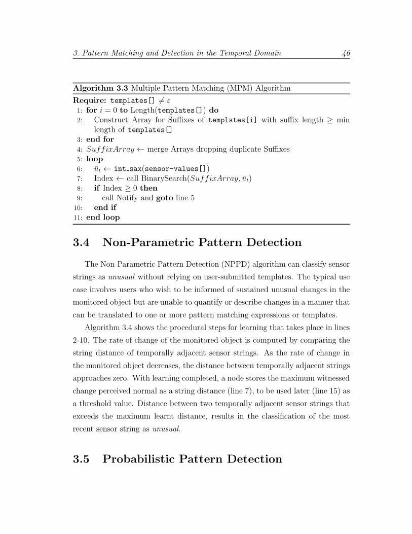
Algorithm 3.3 Multiple Pattern Matching (MPM) Algorithm
Require: templates[] 6= ε1: for i = 0 to Length(templates[]) do2: Construct Array for Suffixes of templates[i] with suffix length ≥ min
length of templates[]3: end for4: SuffixArray ← merge Arrays dropping duplicate Suffixes5: loop6: ut ← int sax(sensor-values[])7: Index ← call BinarySearch(SuffixArray, ut)8: if Index ≥ 0 then9: call Notify and goto line 510: end if11: end loop
3.4 Non-Parametric Pattern Detection
The Non-Parametric Pattern Detection (NPPD) algorithm can classify sensor
strings as unusual without relying on user-submitted templates. The typical use
case involves users who wish to be informed of sustained unusual changes in the
monitored object but are unable to quantify or describe changes in a manner that
can be translated to one or more pattern matching expressions or templates.
Algorithm 3.4 shows the procedural steps for learning that takes place in lines
2-10. The rate of change of the monitored object is computed by comparing the
string distance of temporally adjacent sensor strings. As the rate of change in
the monitored object decreases, the distance between temporally adjacent strings
approaches zero. With learning completed, a node stores the maximum witnessed
change perceived normal as a string distance (line 7), to be used later (line 15) as
a threshold value. Distance between two temporally adjacent sensor strings that
exceeds the maximum learnt distance, results in the classification of the most
recent sensor string as unusual.
3.5 Probabilistic Pattern Detection

3. Pattern Matching and Detection in the Temporal Domain 47
Algorithm 3.4 Non-Parametric Pattern Detection (NPPD) Algorithm
Require: learnPeriod 6= ε1: maxδ, learnCounter← 02: while learnCounter ≤ learnPeriod do3: ut ← int sax(sensor-valuest[])
{sensor-valuest is a window with the most recent observations}4: ut−1 ← int sax(sensor-valuest−1[])
{sensor-valuest−1 is a window temporally shifted by one time unit}5: δ ← ‖ut − ut−1‖S6: if δ > maxδ then7: maxδ ← δ8: end if9: Increment learnCounter by 110: end while11: loop12: ut ← int sax(sensor-valuest[])13: ut−1 ← int sax(sensor-valuest−1[])14: δ ← ‖ut − ut−1‖S15: if δ > maxδ then16: call Notify and goto line 11 {Current distance is greater than max dis-
tance learnt}17: end if18: end loop
Probabilistic Pattern Detection (PPD) (Algorithm 3.5) is procedurally similar
to non-parametric detection, in that it also undergoes a learning phase. The
difference is that PPD does not employ the distance metric of Equation 3.2 to
determine similarity between strings. Instead, it relies on a Markov model to
compute the probability of occurrence of a sensor string, given symbol transitions
observed during training.
PPD handles symbolic conversion as a Markov process where the set of states
equals the size of the alphabet. If the process outputs ui at time t and then moves
to uj at time t + 1, the probability for this transition is represented by pij and
a state transition from state i to j is observed. To encode symbol transitions, a
square matrix called the transition matrix is populated. For simplicity, we employ
a Markov chain of order one, however higher order (memory) Markov chains can

3. Pattern Matching and Detection in the Temporal Domain 48
Algorithm 3.5 Probabilistic Pattern Detection (PPD) Algorithm
Require: learnPeriod, θ 6= ε1: learnCounter← 02: TransitionMatrix[][]← 03: while learnCounter ≤ learnPeriod do4: u← int sax(sensor-values[])5: for i = 0 to |u| do6: Update TransitionMatrix[][] {Update state transition probabilities}7: end for8: Increment learnCounter by 19: end while10: loop11: ut ← int sax(sensor-values[])12: if P (ut) ≤ θ then13: call Notify and goto line 1014: end if15: end loop
be used.
Path probabilities are computed using the Markov model built during the
learning phase (line 12). A path probability is a realisation of a Markov chain
as a path in time through its state space [Nor97]. Such a probability for path
(u1, u2 . . . ut) is given by:
P (ut) = pu1u2pu2u3 . . . put−1ut
A zero probability for a sensor string results in its classification as unusual
since the individual transitions in the string were improbable, given the learning
data that populated the transition matrix.
3.6 Summary
In this chapter we introduced a collection of algorithms that provide pattern
matching and detection functionality. The basis for the algorithms is SAX, a
symbolic conversion method employed to transform sliding windows of sensor

3. Pattern Matching and Detection in the Temporal Domain 49
observations to strings such that pattern matching and detection can be accom-
plished using the strings alone.
The proposed algorithms cater for the following situations:
(i) Exact pattern matching, that matches a sensor string against a user sub-
mitted template.
(ii) Approximate pattern matching, that offers similarity searches between sen-
sor strings and templates.
(iii) Multiple pattern matching, that implements exact pattern matching with
theoretical search efficiency when the cumulative length of templates is much
larger than the sensor string.
(iv) Non-parametric pattern detection, that learns the normal rate of change be-
tween temporally adjacent sensor strings, and uses it to classify new strings
as normal or unusual.
(v) Probabilistic pattern detection, similar to the above, classifies a sensor string
according to the path probability of the string given a transition matrix
populated during learning.
In the next chapter we evaluate the performance of our algorithms, with re-
spect to true and false positives, in real world sensor data sets.
Chapter 4
Temporal Algorithms: Evaluation
through Emulation
In this chapter, we initiate the performance evaluation of the pattern matching
and detection algorithms introduced in Chapter 3. The aim is twofold: first,
to assess matching and detection accuracy across a selection of real-world sen-
sor data and different choice of algorithm parameters, and second, to compare
the algorithms with competitive methods for event detection. Evaluation is per-
formed by emulation, a type of simulation where a computer program imitates
functions of another device [Jai91], in our case a WSN node — we defer discussion
of practical evaluation through deployment to Chapter 5.
We begin with a discussion of methodology and experimental setup in Section
4.1 which is common across all the experiments described in this chapter. We
categorise experiments in three broad case studies (Sections 4.2 to 4.4) examining
data from different sensors and summarise findings in Section 4.5.
4.1 Methodology and Experimental Setup
We emulate the data acquisition process as it would be typically implemented in
a WSN setting: sensors are sampled at a specific (configurable) frequency and
observations are processed by our algorithms. The sequence, shown in Figure 4.1,
50
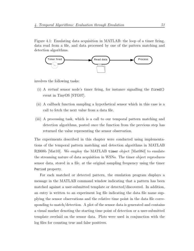
4. Temporal Algorithms: Evaluation through Emulation 51
Figure 4.1: Emulating data acquisition in MATLAB: the loop of a timer firing,data read from a file, and data processed by one of the pattern matching anddetection algorithms.
Timer fired Read data Process
involves the following tasks:
(i) A virtual sensor node’s timer firing, for instance signalling the fired()
event in TinyOS [STG07].
(ii) A callback function sampling a hypothetical sensor which in this case is a
call to fetch the next value from a data file.
(iii) A processing task, which is a call to our temporal pattern matching and
detection algorithms, posted once the function from the previous step has
returned the value representing the sensor observation.
The experiments described in this chapter were conducted using implementa-
tions of the temporal pattern matching and detection algorithms in MATLAB
R2008b [Mat10]. We employ the MATLAB timer object [Mat08d] to emulate
the streaming nature of data acquisition in WSNs. The timer object reproduces
sensor data, stored in a file, at the original sampling frequency using the timer
Period property.
For each matched or detected pattern, the emulation program displays a
message in the MATLAB command window indicating that a pattern has been
matched against a user-submitted template or detected/discovered. In addition,
an entry is written to an experiment log file indicating the data file name sup-
plying the sensor observations and the relative time point in the data file corre-
sponding to match/detection. A plot of the sensor data is generated and contains
a visual marker denoting the starting time point of detection or a user-submitted
template overlaid on the sensor data. Plots were used in conjunction with the
log files for counting true and false positives.
4. Temporal Algorithms: Evaluation through Emulation 52
To validate the emulated implementation in MATLAB, experiments were re-
produced on the WSN-specific TOSSIM [LLWC03] simulator. Verification was
performed by tasking a TOSSIM-simulated node to execute the same steps as the
MATLAB program and confirm pattern classification by displaying the relative
timestamp (in timer ticks) of match/detection on the command window. This
process confirmed that the relative time point of match/detection by MATLAB
emulation was identical with that reported by TOSSIM.
4.2 Case Study 1: Indoor Deployment
The experiments of this case study were conducted on data from the indoor
deployment [Int04] of 54 nodes at the Intel Lab, Berkeley. This data set was
selected for the following reasons:
• It is representative of the class of applications we are targeting with char-
acteristics specific to indoor deployments.
• It contains imperfections, in the form of outliers and missing values, that
were not corrected to assess detection performance under realistic data char-
acteristics.
The data set contains approximately 2.3 million observations of temperature,
humidity, light, and voltage sampled at a frequency of 0.031Hz. The data is
made available as a single file with timestamped observations.
4.2.1 Evaluation of Exact and Approximate Matching
In this section we evaluate Algorithms 3.1 and 3.2 which require the input of
a specific template pattern by a user for matching against strings obtained by
symbolic conversion of the sensor stream.
4. Temporal Algorithms: Evaluation through Emulation 53
Metric
We employ the mean number of false positives per node to characterise the impact
of symbolic conversion parameters to the number of incorrect pattern matches
reported by the exact and approximate matching algorithms of Chapter 3.
Hypothesis
There are values of symbolic conversion parameters — alphabet size, window
length and compression ratio — that reduce false positives reported by the exact
and approximate pattern matching algorithms, on data from different sensors.
Experiments
For this series of experiments, the data set was divided to observations per node
in order to emulate data acquisition in MATLAB in the manner described pre-
viously. To simulate users interested in pattern events, template patterns were
supplied by extracting sequences of data and providing them as input to the algo-
rithms for matching. An example of a user-submitted template pattern employed
in the experiments is the sustained increase in temperature observed between
7.00 am and 7.20 am, possibly due to the effect of sunrise or automated heating
system.
The expected behaviour of exact pattern matching is to identify an occurrence
of the user-submitted template pattern. As described in Section 3.2, the algorithm
positively matches a sensor string to the template pattern when the distance
between the two strings is zero. False positives are counted when the exact pattern
matching algorithm produces a zero distance between the template pattern and
a sensor string that does not correspond to the template pattern. Using the early
morning sustained increase in temperature as a template pattern example, a false
positive is counted if the algorithm matches with zero distance this template to
a sensor string from a different time of day.
4. Temporal Algorithms: Evaluation through Emulation 54
The expected behaviour of approximate matching is to identify similarities be-
tween user supplied template patterns and sensor strings. This translates to pos-
itively matching a sensor string to a template pattern when the distance between
them is zero or below a user-supplied threshold. This user-supplied threshold
determines the desired similarity between the template and the sensor strings.
For the purpose of the experiment, appropriate values for thresholds were se-
lected by specifying that the template pattern and the sensor string can have
up to 10% of their symbols at most 2 characters apart. For instance, in this
experiments the template pattern “aabbccddee“ would approximately match the
sensor string “abbbccddde“, with their character differences highlighted in bold
typeface. A false positive is counted when the algorithm matches with distance
below the threshold a pattern template to a sensor string from a different time
of day. Figures 4.2a and 4.2b show examples of approximate pattern matching
with windows of varying sizes.
The experiment was conducted over temperature, humidity, light, and voltage
sensor data and different symbolic conversion parameter values were explored.
Specifically, input window lengths of 28, 40, 160, 496, 836 and 1260 were tested
as these values represent a choice likely to cater for a variety of both short and
long duration pattern events. Finally, a range of symbolic conversion compression
ratios (1/1, 2/1, 4/1, and 6/1) and alphabets (5, 10, 15 and 20 characters) were
tested to explore the effect of string approximation information content to false
positives.
Findings
The main finding of this experiment is that the number of false positives reported
by the exact and approximate pattern matching algorithms depend on symbolic
conversion parameters such as compression ratio, input window length and type
of sensor data. For instance, Table 4.1 shows that increasing the window length
from 40 sensor readings to 160 sensor readings with a symbolic compression ratio
of 2/1, reduces false positives from 13 to 3. We believe that this is a positive
result as three false positive reports in a 30-day deployment period incurs only a

4. Temporal Algorithms: Evaluation through Emulation 55
Window length Comp. Ratio40 160 486 836
Mean False Positives
Alphabet Size 511 6 2 0 None17 8 4 2 2/134 29 26 23 4/1
Alphabet Size 102 1 0 0 None13 3 3 1 2/122 16 15 9 4/1
Alphabet Size 151 1 0 0 None13 3 3 1 2/121 16 16 9 4/1
Table 4.1: Relationship of alphabet size, window length and compression ratiowith the mean number of false positives (per node) reported by the ApproximatePattern Matching (APM) algorithm on the temperature attribute over a data setspanning a period of 30 days.
moderate use of the radio, for instance only three notifications transmitted.
We find that longer windows are necessary in order to reduce false positives for
data with less smooth changes such as light. The average values of false positives
over the light attribute are shown on Table 4.2 and their relationship to window
length is in agreement with the observations made in [KLF05], in particular the
view that larger windows are necessary for data with a high degree of variability.
Moreover, increasing the alphabet size above 10 characters does not significantly
reduce the number of false positives.
Overall, our hypothesis was confirmed as there are certain symbolic conversion
parameter values that reduce the number of false positives. Specifically, we settle
on an alphabet size of 10 characters, compression ratio of 2/1 or 4/1 and input
window lengths of 40 and above. Although the pattern matching algorithms can
use default values for these parameters, there is some benefit for users who choose
to fine tune compression ratio and window length — either at pre-deployment or
at runtime — according to characteristics of the sensed data such as variability
and sampling frequency.

4. Temporal Algorithms: Evaluation through Emulation 56
Window length Comp. Ratio40 160 486 836
Mean False Positives
Alphabet Size 567 55 32 6 None113 98 67 29 2/1119 101 74 34 4/1
Alphabet Size 1044 37 16 5 None87 66 41 18 2/191 72 50 28 4/1
Alphabet Size 1544 37 16 3 None79 64 41 18 2/190 72 49 28 4/1
Table 4.2: Relationship of alphabet size, window length and compression ratiowith the mean number of false positives (per node) reported by the Exact PatternMatching (EPM) algorithm on the light attribute over a data set spanning aperiod of 30 days.
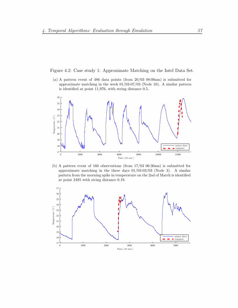
4. Temporal Algorithms: Evaluation through Emulation 57
Figure 4.2: Case study 1: Approximate Matching on the Intel Data Set.
(a) A pattern event of 486 data points (from 20/03 08:00am) is submitted forapproximate matching in the week 01/03-07/03 (Node 10). A similar patternis identified at point 11,976, with string distance 0.5.
0 2000 4000 6000 8000 10000 1200017
18
19
20
21
22
23
24
25
26
Time [ 32 secs ]
Tem
per
atu
re[C
]
sensor datatemplate
(b) A pattern event of 160 observations (from 17/03 06:30am) is submitted forapproximate matching in the three days 01/03-03/03 (Node 3). A similarpattern from the morning spike in temperature on the 2nd of March is identifiedat point 2485 with string distance 0.19.
0 1000 2000 3000 4000 500017
18
19
20
21
22
23
24
25
26
27
Time [ 32 secs ]
Tem
per
atu
re[C
]
sensor datatemplate
4. Temporal Algorithms: Evaluation through Emulation 58
4.3 Case Study 2: Seismic and Acoustic Data
The purpose of this case study is to conduct an accuracy comparison of the
Non-Parametric Pattern Detection (NPPD) algorithm with two alternative tech-
niques, and to perform a preliminary study of the effects of measurement noise
to detection accuracy.
The experiments were carried out on data from the volcanic monitoring de-
ployment [WALJ+06] at Reventador, an active volcano in Ecuador. The data set
was selected for the following reasons:
• It is also representative of a class of reactive environmental applications
aimed at detecting unusual activity, which is a good fit with our research
goals.
• It contains a large number of pattern events recorded in two sensing modal-
ities: seismic and acoustic.
According to [WALJ+06], the deployment comprised 16 sensor nodes that sam-
pled seismic and acoustic data at a frequency of 100Hz for a 19-day period in
2005. The data is made available as a collection of 1, 209 files out of which we
identified 947 contained pattern events while the rest were either data segments
without unusual patterns or noise possibly due to faulty sensors. Each file in-
cludes a header section with the timestamps of the data sample including the
time length of the pattern event.
4.3.1 Evaluation of Non-Parametric Pattern Detection
The experiments of this section compare the accuracy of the Non-Parametric
Pattern Detection (NPPD) algorithm (Section 3.4) against two competitive tech-
niques:
• Exponentially Weighted Moving Average (EWMA) according to the imple-
mentation details described in [WALJ+06].
4. Temporal Algorithms: Evaluation through Emulation 59
• Real-time Seismic Amplitude Measurement (RSAM), which is an alternative
method for detecting unusual volcanic activity [EM91].
The first technique was employed by the researchers who carried out the data
collection while the second technique is an alternative method for measuring
volcanic activity.
Metrics
To characterise the accuracy of the pattern detection algorithm with respect to
true positives, we employ the sensitivity [WF05] metric given by:
S =TP
TP + FN, (4.1)
where TP is the total number of true positives classified by a pattern matching
and detection method and FN is the total number of false negatives. In addition,
we use the false positive rate which is given by:
FPR =FP
TP + FN, (4.2)
where FP is the total number of false positives or patterns misclassified as unusual
by our algorithm.
Hypothesis
The Non-Parametric Pattern Detection (NPPD) algorithm (Section 3.4) can per-
form competitively against EWMA and RSAM.
Experiments
The process followed measures the accuracy of NPPD by counting the number of
true and false pattern event occurrences reported by the algorithm and comparing
it against the corresponding figures for EWMA and RSAM. To investigate the
impact of algorithmic parameters to pattern detection accuracy we conduct the
4. Temporal Algorithms: Evaluation through Emulation 60
experiments using two settings: high sensitivity aiming to make pattern detection
more sensitive to seismic events of relatively small magnitude and low sensitivity
for detecting seismic disturbances of relatively higher magnitude. For NPPD
the choice of high/low sensitivity was represented by the symbolic conversion
compression ratios of 2/1 and 4/1. In the case of EWMA and RSAM, high/low
sensitivity was implemented by selecting different values for the thresholds.
For this case study, NPPD uses a window length of 128 readings and a 10-
letter alphabet. The values for these parameters relate to the symbolic conversion
component of the NPPD algorithm and were obtained during earlier empirical
studies, discussed in Section 4.2.1. The NPPD algorithm was trained on a subse-
quence of 1, 024 data points that did not contain any pattern events. Distances
were computed using Equation 3.2 for the comparison of adjacent strings ob-
tained by transforming temporally adjacent numeric sensor observations using
the algorithm of Section 3.4.
Both EWMA and RSAM rely on a threshold to determine whether the un-
derlying activity of the monitored process is unusual. In the case of EWMA, the
ratio of two exponentially-weighted moving averages (EWMAs) over the input
signal is compared to the threshold. The short-term average (STA) contained 30
observations, the long-term average (LTA) contained 300 observations and the
threshold was set to 0.3 and to 0.25 to represent low and high sensitivity respec-
tively. We obtained values for STA/LTA window lengths, weights and thresholds
empirically after testing numerous alternatives on a 1/4 of the data 1.
RSAM [EM91] is similar to EWMA, but instead of operating on ratios of
averages it sums the mean amplitude of the signal during a given interval to
provide a measure of the level of activity. When the RSAM amplitude exceeds a
threshold an event is triggered. We employed an interval of 3, 000 observations
and thresholds of 0.02 and 0.01 to represent low and high sensitivity respectively.
1We attempted to communicate with the authors of the original work [WALJ+06,WADHW08] to enquire about their choice of parameter values but unfortunately we did notreceive a reply.
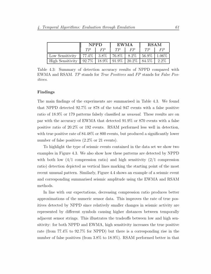
4. Temporal Algorithms: Evaluation through Emulation 61
NPPD EWMA RSAMTP FP TP FP TP FP
Low Sensitivity 77.4% 3.8% 76.8% 8.2% 56.9% 1.06%High Sensitivity 92.7% 18.9% 91.9% 20.2% 84.5% 2.2%
Table 4.3: Summary of detection accuracy results of NPPD compared withEWMA and RSAM. TP stands for True Positives and FP stands for False Pos-itives.
Findings
The main findings of the experiments are summarised in Table 4.3. We found
that NPPD detected 92.7% or 878 of the total 947 events with a false positive
ratio of 18.9% or 179 patterns falsely classified as unusual. These results are on
par with the accuracy of EWMA that detected 91.9% or 870 events with a false
positive ratio of 20.2% or 192 events. RSAM performed less well in detection,
with true positive rate of 84.48% or 800 events, but produced a significantly lower
number of false positives (2.2% or 21 events).
To highlight the type of seismic events contained in the data set we show two
examples in Figure 4.3. We also show how these patterns are detected by NPPD
with both low (4/1 compression ratio) and high sensitivity (2/1 compression
ratio) detection depicted as vertical lines marking the starting point of the most
recent unusual pattern. Similarly, Figure 4.4 shows an example of a seismic event
and corresponding summarised seismic amplitude using the EWMA and RSAM
methods.
In line with our expectations, decreasing compression ratio produces better
approximations of the numeric sensor data. This improves the rate of true pos-
itives detected by NPPD since relatively smaller changes in seismic activity are
represented by different symbols causing higher distances between temporally
adjacent sensor strings. This illustrates the tradeoffs between low and high sen-
sitivity: for both NPPD and EWMA, high sensitivity increases the true positive
rate (from 77.4% to 92.7% for NPPD) but there is a corresponding rise in the
number of false positives (from 3.8% to 18.9%). RSAM performed better in that
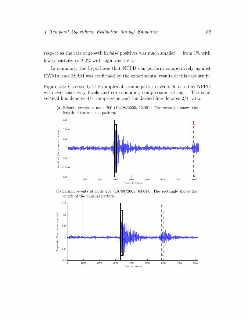
4. Temporal Algorithms: Evaluation through Emulation 62
respect as the rate of growth in false positives was much smaller — from 1% with
low sensitivity to 2.2% with high sensitivity.
In summary, the hypothesis that NPPD can perform competitively against
EWMA and RSAM was confirmed by the experimental results of this case study.
Figure 4.3: Case study 2: Examples of seismic pattern events detected by NPPDwith two sensitivity levels and corresponding compression settings. The solidvertical line denotes 4/1 compression and the dashed line denotes 2/1 ratio.
(a) Seismic events at node 200 (13/08/2005, 12.29). The rectangle shows thelength of the unusual pattern.
0 1000 2000 3000 4000 5000 6000 7000 8000−0.06
−0.04
−0.02
0
0.02
0.04
0.06
Time [ 1/100 sec]
Am
plitu
de
[N
orm
.se
nso
rre
sponse
]
(b) Seismic events at node 209 (16/08/2005, 04.04). The rectangle shows thelength of the unusual pattern.
0 1000 2000 3000 4000 5000 6000 7000 8000−0.1
−0.05
0
0.05
0.1
0.15
Time [ 1/100 sec]
Am
plitu
de
[N
orm
.se
nso
rre
sponse
]
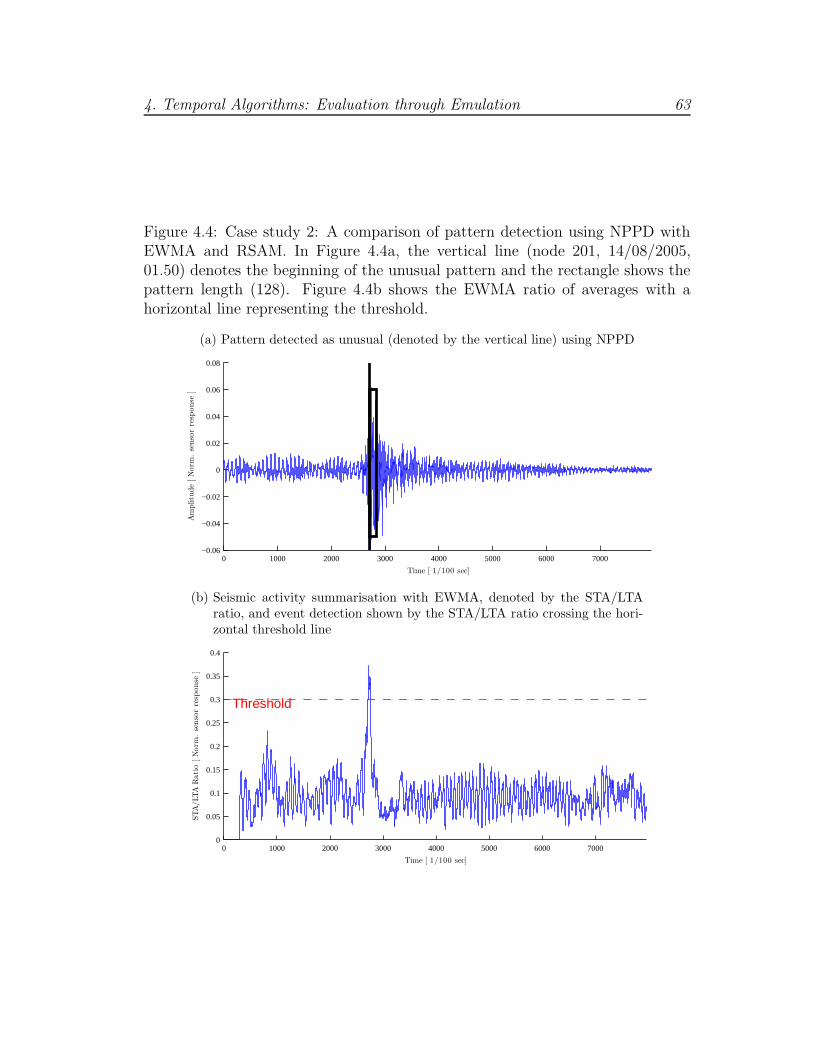
4. Temporal Algorithms: Evaluation through Emulation 63
Figure 4.4: Case study 2: A comparison of pattern detection using NPPD withEWMA and RSAM. In Figure 4.4a, the vertical line (node 201, 14/08/2005,01.50) denotes the beginning of the unusual pattern and the rectangle shows thepattern length (128). Figure 4.4b shows the EWMA ratio of averages with ahorizontal line representing the threshold.
(a) Pattern detected as unusual (denoted by the vertical line) using NPPD
0 1000 2000 3000 4000 5000 6000 7000−0.06
−0.04
−0.02
0
0.02
0.04
0.06
0.08
Time [ 1/100 sec]
Am
plitu
de
[N
orm
.se
nso
rre
sponse
]
(b) Seismic activity summarisation with EWMA, denoted by the STA/LTAratio, and event detection shown by the STA/LTA ratio crossing the hori-zontal threshold line
0 1000 2000 3000 4000 5000 6000 70000
0.05
0.1
0.15
0.2
0.25
0.3
0.35
0.4
Time [ 1/100 sec]
STA
/LT
AR
ati
o[N
orm
.se
nso
rre
sponse
]
Threshold
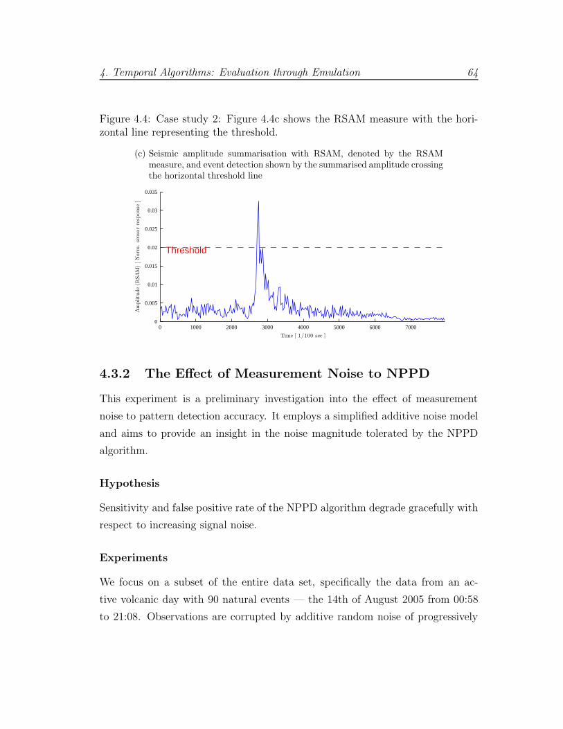
4. Temporal Algorithms: Evaluation through Emulation 64
Figure 4.4: Case study 2: Figure 4.4c shows the RSAM measure with the hori-zontal line representing the threshold.
(c) Seismic amplitude summarisation with RSAM, denoted by the RSAMmeasure, and event detection shown by the summarised amplitude crossingthe horizontal threshold line
0 1000 2000 3000 4000 5000 6000 70000
0.005
0.01
0.015
0.02
0.025
0.03
0.035
Time [ 1/100 sec ]
Am
plitu
de
(RSA
M)
[N
orm
.se
nso
rre
sponse
]
Threshold
4.3.2 The Effect of Measurement Noise to NPPD
This experiment is a preliminary investigation into the effect of measurement
noise to pattern detection accuracy. It employs a simplified additive noise model
and aims to provide an insight in the noise magnitude tolerated by the NPPD
algorithm.
Hypothesis
Sensitivity and false positive rate of the NPPD algorithm degrade gracefully with
respect to increasing signal noise.
Experiments
We focus on a subset of the entire data set, specifically the data from an ac-
tive volcanic day with 90 natural events — the 14th of August 2005 from 00:58
to 21:08. Observations are corrupted by additive random noise of progressively
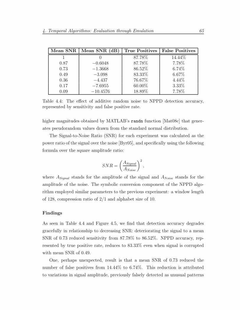
4. Temporal Algorithms: Evaluation through Emulation 65
Mean SNR Mean SNR (dB) True Positives False Positives
1 0 87.78% 14.44%0.87 −0.6048 87.78% 7.78%0.73 −1.3668 86.52% 6.74%0.49 −3.098 83.33% 6.67%0.36 −4.437 76.67% 4.44%0.17 −7.6955 60.00% 3.33%0.09 −10.4576 18.89% 7.78%
Table 4.4: The effect of additive random noise to NPPD detection accuracy,represented by sensitivity and false positive rate.
higher magnitudes obtained by MATLAB’s randn function [Mat08c] that gener-
ates pseudorandom values drawn from the standard normal distribution.
The Signal-to-Noise Ratio (SNR) for each experiment was calculated as the
power ratio of the signal over the noise [Byr05], and specifically using the following
formula over the square amplitude ratio:
SNR =
(
ASignal
ANoise
)2
,
where ASignal stands for the amplitude of the signal and ANoise stands for the
amplitude of the noise. The symbolic conversion component of the NPPD algo-
rithm employed similar parameters to the previous experiment: a window length
of 128, compression ratio of 2/1 and alphabet size of 10.
Findings
As seen in Table 4.4 and Figure 4.5, we find that detection accuracy degrades
gracefully in relationship to decreasing SNR: deteriorating the signal to a mean
SNR of 0.73 reduced sensitivity from 87.78% to 86.52%. NPPD accuracy, rep-
resented by true positive rate, reduces to 83.33% even when signal is corrupted
with mean SNR of 0.49.
One, perhaps unexpected, result is that a mean SNR of 0.73 reduced the
number of false positives from 14.44% to 6.74%. This reduction is attributed
to variations in signal amplitude, previously falsely detected as unusual patterns
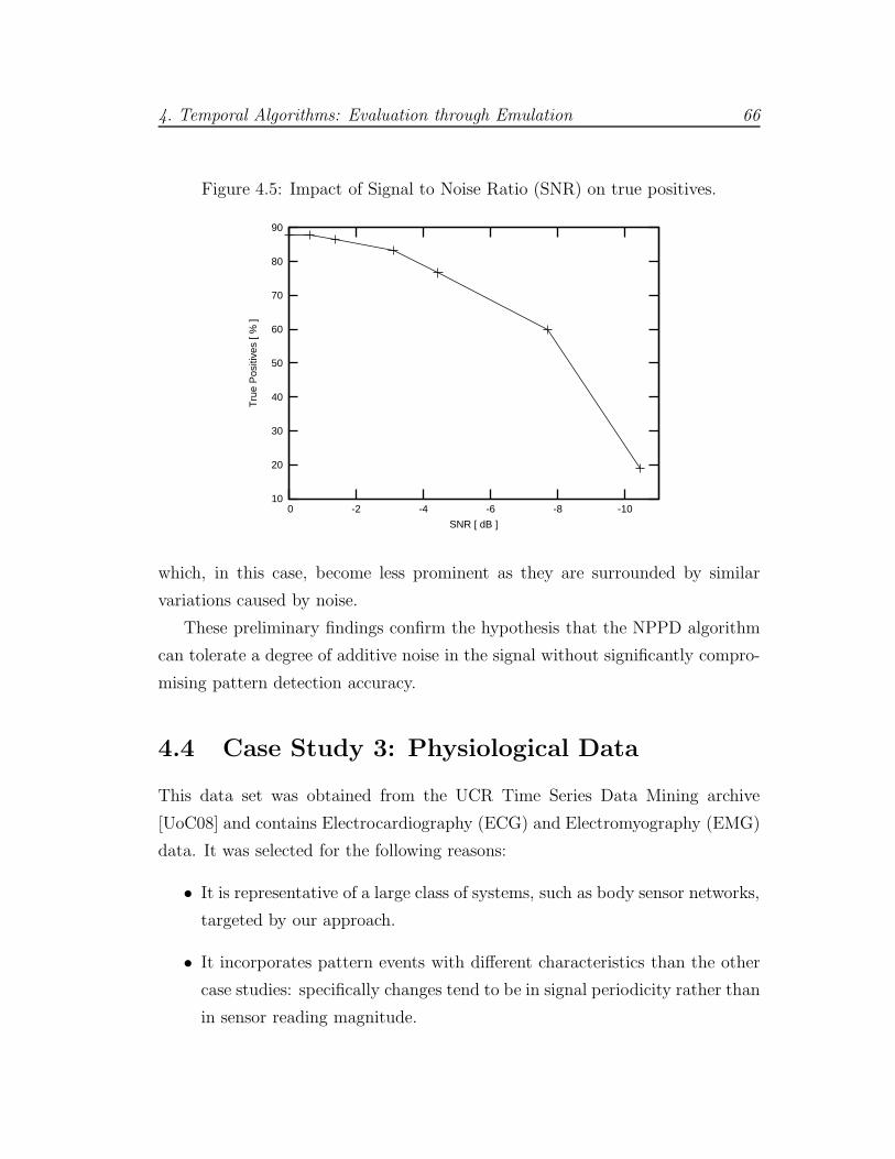
4. Temporal Algorithms: Evaluation through Emulation 66
Figure 4.5: Impact of Signal to Noise Ratio (SNR) on true positives.
10
20
30
40
50
60
70
80
90
-10-8-6-4-2 0
Tru
e P
ositi
ves
[ % ]
SNR [ dB ]
which, in this case, become less prominent as they are surrounded by similar
variations caused by noise.
These preliminary findings confirm the hypothesis that the NPPD algorithm
can tolerate a degree of additive noise in the signal without significantly compro-
mising pattern detection accuracy.
4.4 Case Study 3: Physiological Data
This data set was obtained from the UCR Time Series Data Mining archive
[UoC08] and contains Electrocardiography (ECG) and Electromyography (EMG)
data. It was selected for the following reasons:
• It is representative of a large class of systems, such as body sensor networks,
targeted by our approach.
• It incorporates pattern events with different characteristics than the other
case studies: specifically changes tend to be in signal periodicity rather than
in sensor reading magnitude.
4. Temporal Algorithms: Evaluation through Emulation 67
The ECG data contains segments of 512 normal observations sampled at 128Hz
that change to supraventricular and malignant ventricular — both different types
of arrythmias — for the remaining 512 observations. The EMG data contains two
sets of 30, 000 observations sampled at 1KHz of an athlete’s Gluteus Maximus
activity during the last 30 seconds of a 3 min exercise on a treadmill at 3.72 m/s
for the first set and 4.56 m/s for the second set.
4.4.1 Evaluation of Non-Parametric and Probabilistic Pat-
tern Detection
The purpose of this experiment is to evaluate the detection latency of non-
parametric and probabilistic pattern detection, Algorithms 3.4 and 3.5 of the
previous chapter respectively.
Metric
To characterise the delay in pattern detection, we employ detection latency as
the time elapsed, in seconds, between the starting point of a pattern event and
the time point that the pattern was classified as unusual by the algorithms. This
metric is important in the context of medical applications since timely notifica-
tion of pattern events concerning the health status of a patient can be critical
[MFjWM04].
Hypothesis
Non-parametric and probabilistic algorithms are capable of detecting patterns in
high frequency physiological data with relatively low detection latency.
Experiments
To simulate an ECG pattern event, we append segments from supraventricular
and malignant ventricular ECG data to normal ECG data. There are 18 ECG
segments of normal data, 30 segments of supraventricular and 22 segments of
4. Temporal Algorithms: Evaluation through Emulation 68
malignant ventricular. The experiment tests 52 combinations of normal ECG
changing to either supraventricular or malignant ventricular. For EMG data we
append two sets recording muscular activity from the same athlete on a treadmill
workout with different speed settings.
For NPPD, a window length of 128 observations was used with compression
ratio of 2/1, alphabet size of 10 and training data set to a 1/4 of each data set.
The PPD algorithm does not require any parameters apart from a learn
counter which was set to a 1/4 of each data set or 128 and 7, 500 observations, for
ECG and EMG respectively. Recall that detection occurs when distance between
temporally adjacent strings exceeds the maximum learnt distance in the case of
NPPD, and for PPD, when the path probability for observed strings obtained
from symbolic conversion of numeric observations is equal to zero.
Findings
Table 4.5 summarises the minimum, maximum and average latencies over the
52 ECG experiments. These findings confirm the hypothesis and show relatively
low NPPD mean latency: 0.086 seconds for normal ECG turning to malignant
ventricular and 0.102 seconds for normal ECG turning to supraventricular. Cor-
responding times for the detection latency of the PPD algorithm, were 0.047 and
0.109 seconds. We believe that the worst-case scenario with maximum detection
latency of 0.797 seconds shows a delay that could satisfy bounds of time critical
medical applications.
Examples of pattern detection for ECG data and the NPPD algorithm are
shown in Figures 4.6a (malignant ventricular) and 4.6b (supraventricular).
Due to lack of additional data, the EMG evaluation consisted of only one
experiment where the PPD algorithm flagged a string of length 512 with 0-
probability at time 30.412 shown in Figure 4.7 — a latency of 0.412 seconds.

4. Temporal Algorithms: Evaluation through Emulation 69
Pattern Detection Latency (secs)Min Max Mean
Non Parametric Pattern DetectionNormal ECG chang-ing to Malignant Ven-tricular
0.055 0.492 0.086
Normal ECG chang-ing to Supraventricu-lar
0.062 0.797 0.102
Probabilistic Pattern DetectionNormal ECG chang-ing to Malignant Ven-tricular
0.039 0.156 0.047
Normal ECG chang-ing to Supraventricu-lar
0.07 0.359 0.109
Table 4.5: Minimum, maximum and mean detection latency (in seconds) over 52experiments of NPPD and PPD algorithms on ECG data. Learning counter wasset to 1/4 of the data set, or exactly 1 second. Latency is the elapsed number ofseconds from the time of the pattern event (exactly at 4 seconds) to the time ofdetection.
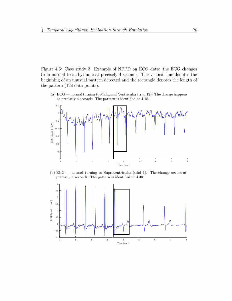
4. Temporal Algorithms: Evaluation through Emulation 70
Figure 4.6: Case study 3: Example of NPPD on ECG data: the ECG changesfrom normal to arrhythmic at precisely 4 seconds. The vertical line denotes thebeginning of an unusual pattern detected and the rectangle denotes the length ofthe pattern (128 data points).
(a) ECG— normal turning to Malignant Ventricular (trial 12). The change happensat precisely 4 seconds. The pattern is identified at 4.18.
0 1 2 3 4 5 6 7 8
−1
−0.8
−0.6
−0.4
−0.2
0
0.2
Time [ sec ]
EC
GSig
nal2
[m
V]
(b) ECG — normal turning to Supraventricular (trial 1). The change occurs atprecisely 4 seconds. The pattern is identified at 4.38.
0 1 2 3 4 5 6 7 8−1
−0.5
0
0.5
1
1.5
2
2.5
3
Time [ sec ]
EC
GSig
nal1
[m
V]
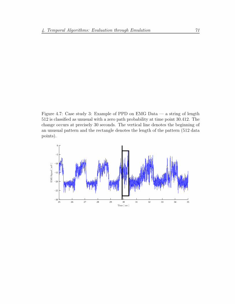
4. Temporal Algorithms: Evaluation through Emulation 71
Figure 4.7: Case study 3: Example of PPD on EMG Data — a string of length512 is classified as unusual with a zero path probability at time point 30.412. Thechange occurs at precisely 30 seconds. The vertical line denotes the beginning ofan unusual pattern and the rectangle denotes the length of the pattern (512 datapoints).
25 26 27 28 29 30 31 32 33 34 35−30
−25
−20
−15
−10
−5
0
Time [ sec ]
EM
GSig
nal[m
V]

4. Temporal Algorithms: Evaluation through Emulation 72
4.5 Summary of Findings
We conducted evaluation of the temporal pattern matching and detection algo-
rithms on three data sets and the following eight sensing modalities: seismic,
acoustic, temperature, humidity, voltage, light, ECG and EMG. The data sets
were selected to represent target reactive applications that can benefit from pat-
tern matching and detection functionality.
We found the following:
(i) Symbolic conversion parameter values play a role in the number of false pos-
itives reported by the exact and approximate pattern matching algorithms.
Longer input windows reduce false positives especially on data with a high
degree of variability.
(ii) The non-parametric pattern detection algorithm is competitive with other
techniques such as EWMA and RSAM. NPPD provides higher detection
sensitivity (true positive rate) than both EWMA and RSAM.
(iii) NPPD sensitivity degrades gracefully with respect to increasing signal noise:
detection accuracy remains over 80% even with a mean SNR of 0.49.
(iv) Both NPPD and PPD algorithms show relatively low detection latency —
approximately a tenth of a second on average — on physiological data such
as ECG and EMG.
We continue the evaluation of the temporal algorithms in the next chapter with
a discussion of findings obtained through deployment.
Chapter 5
Temporal Algorithms: Evaluation
through Deployment
This chapter analyses the runtime behaviour and operational profile of the pro-
posed temporal domain algorithms, and shows their suitability for the extremely
resource constrained execution platform through deployment on real WSNs.
First, Section 5.1 demonstrates execution efficiency through measurement of
the algorithms’ runtime on WSN nodes. Second, Section 5.2 introduces a dynamic
sampling frequency management method that allows nodes to reduce MCU work-
load during periods of inactivity. Third, Section 5.3 describes integration with a
Publish/Subscribe system that provides the user interface to the pattern match-
ing and detection algorithms. Finally, Section 5.4 illustrates suitability for a
novel type of node that lacks on-board power source and Section 5.5 summarises
findings from deployments.
5.1 Execution Profile of Temporal Domain Al-
gorithms
The vast majority of extremely resource constrained WSN nodes lack floating
point units (FPUs) forcing floating point operations to be executed in software
73
5. Temporal Algorithms: Evaluation through Deployment 74
penalising performance and accuracy of arithmetic results [Gol91, Hig02]. The
floating point arithmetic impact identified in conventional computing as capable
of reducing system performance by half [OF02], is magnified in WSNs since apart
from affecting performance it can consequently reduce useful node lifetime.
Motivated by the dependence of symbolic conversion and distance calculation
components of the temporal algorithms on floating-point operations, we initiated
a study into their execution profile. We identify the cost of floating point oper-
ations involved in the temporal algorithms, and we refactor such that they use
exclusively integer arithmetic. To this effect, we employ a combination of scal-
ing, fixed-point arithmetic, bitwise techniques and related optimisations such as
loop unrolling. In the following sections, we show the runtime savings achieved
through the application of these techniques. A detailed discussion of methods
and techniques employed can be found in [ZR09d].
Timing measurements reported in this chapter are collected on TMote Sky/
TelosB [Sen08] nodes running TinyOS 2 [LBC+08] applications compiled with
msp430-gcc 3.2.3. Execution times are measured at entry and exit points of
functions with the Timer [STG07] component of TinyOS and specifically the
startOneShot and stop commands. Elapsed execution times for blocks of code
under investigation are reported using the TinyOS printf library.
5.1.1 Refactoring of Pattern Matching and Detection Al-
gorithms
The purpose of this experiment is to profile the pattern matching and detection
algorithms in order to show that they are suitable for extremely resource con-
strained WSN nodes. For reference, we first identify (Appendix C) the relative
cost of different arithmetic operations on the target platform. The outcome is a
timing model (cf. Table C.1) used as a guide in the software development process
of the integer-only pattern matching and detection algorithms.
5. Temporal Algorithms: Evaluation through Deployment 75
Metrics
The execution profile of the pattern matching and detection algorithms is char-
acterised by:
• Total processing runtime (in milliseconds) required by the pattern matching
and detection algorithms.
• Total RAM usage (in bytes) occupied by the program image.
Hypothesis
There are significant runtime savings to be gained from the application of inte-
ger arithmetic combined with related optimisations to the pattern matching and
detection algorithms.
Experiments
We compare the execution time required for our temporal algorithms between
floating point and integer arithmetic implementations. We use an alphabet of 10
characters and compression ratio of 2/1, as these are typical parameter choices
established in the last chapter. Time requirements for exact and approximate
matching are identical since they involve the same procedural steps.
For the Multiple Pattern Matching (MPM) algorithm, we implement a lin-
ear search algorithm (cf. [Gus97] for a description of linear search algorithms
on strings) as a basis for comparison with respect to search costs, for example
searching whether a sensor string exists among a collection of user submitted
templates. We collect timing measurements for MPM from nodes that produce
strings of length 20 from numeric sensor observations of length 40.
We begin our analysis by profiling operations, through execution time mea-
surement, involved in a floating-point implementation of the pattern matching
algorithm. The execution profile shows that the larger share of processing time
is attributed to normalisation of numeric sensor values according to the formula:
5. Temporal Algorithms: Evaluation through Deployment 76
ui − µ
σ
where µ is the mean and σ is the standard deviation of the sequence of numeric
sensor values u. To reduce this cost attributed to floating point division and
subtraction, we replace floats with integers and eliminate division altogether. In-
stead, we scale1 the row of breakpoints — (Table 3.1, in Chapter 3) corresponding
to alphabet size — by integer σ. To operate on numbers of the same magnitude,
we multiply the intermediate Piecewise Aggregate Approximation (PAA) repre-
sentation by the same scaling factor. The number of multiplications required,
is equal to the length of the resulting string representation. Scaling the break-
points involves 10 — the length of breakpoints and typical size of alphabet —
multiplications compared to 40 or more — the length of the numeric sequence —
divisions previously required to standardise u.
We introduce an integer square root is for computation of standard deviation
σ. Substituting integer square root for operating on numbers of higher magnitude
requiring 64-bit types is a costly decision according to Table C.1 (Appendix C)
which shows 64-bit division requiring almost as much MCU time as floating point
division. With integer square root and the maximum value produced by the
Analog-to-Digital Converter (ADC), 32-bit numbers are sufficient for representing
the maximum values of scaled results.
Findings
The main finding of this experiment is the improved execution time of the in-
teger pattern matching algorithm, shown in Figure 5.1, in comparison with a
floating point implementation. Table 5.1 shows a more detailed account of the
timing measurements for operations involved in a floating-point implementation
of pattern matching. The corresponding timing measurements for the integer-only
implementation of the exact and approximate algorithms are shown in Table 5.2:
1We use binary scaling with a scaling factor of 2048.
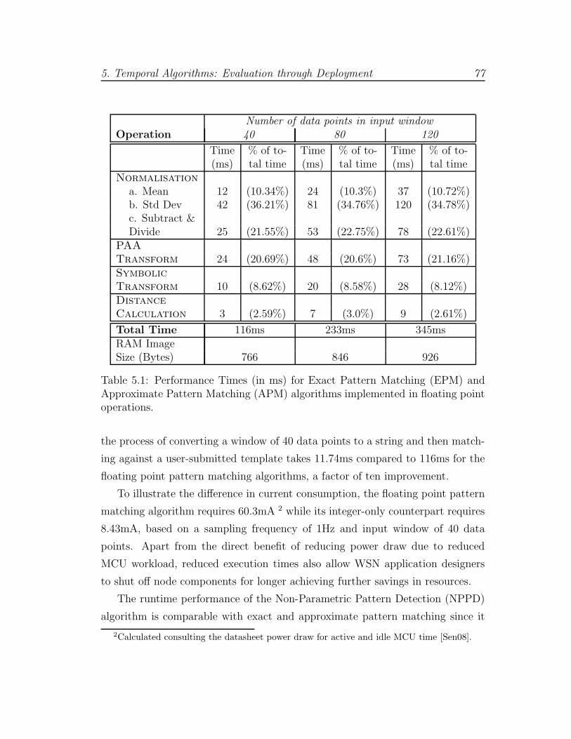
5. Temporal Algorithms: Evaluation through Deployment 77
Number of data points in input windowOperation 40 80 120
Time % of to- Time % of to- Time % of to-(ms) tal time (ms) tal time (ms) tal time
Normalisation
a. Mean 12 (10.34%) 24 (10.3%) 37 (10.72%)b. Std Dev 42 (36.21%) 81 (34.76%) 120 (34.78%)c. Subtract &Divide 25 (21.55%) 53 (22.75%) 78 (22.61%)
PAA
Transform 24 (20.69%) 48 (20.6%) 73 (21.16%)Symbolic
Transform 10 (8.62%) 20 (8.58%) 28 (8.12%)Distance
Calculation 3 (2.59%) 7 (3.0%) 9 (2.61%)
Total Time 116ms 233ms 345msRAM ImageSize (Bytes) 766 846 926
Table 5.1: Performance Times (in ms) for Exact Pattern Matching (EPM) andApproximate Pattern Matching (APM) algorithms implemented in floating pointoperations.
the process of converting a window of 40 data points to a string and then match-
ing against a user-submitted template takes 11.74ms compared to 116ms for the
floating point pattern matching algorithms, a factor of ten improvement.
To illustrate the difference in current consumption, the floating point pattern
matching algorithm requires 60.3mA 2 while its integer-only counterpart requires
8.43mA, based on a sampling frequency of 1Hz and input window of 40 data
points. Apart from the direct benefit of reducing power draw due to reduced
MCU workload, reduced execution times also allow WSN application designers
to shut off node components for longer achieving further savings in resources.
The runtime performance of the Non-Parametric Pattern Detection (NPPD)
algorithm is comparable with exact and approximate pattern matching since it
2Calculated consulting the datasheet power draw for active and idle MCU time [Sen08].
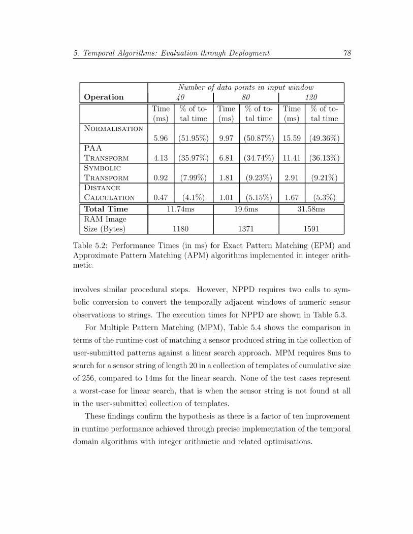
5. Temporal Algorithms: Evaluation through Deployment 78
Number of data points in input windowOperation 40 80 120
Time % of to- Time % of to- Time % of to-(ms) tal time (ms) tal time (ms) tal time
Normalisation
5.96 (51.95%) 9.97 (50.87%) 15.59 (49.36%)PAA
Transform 4.13 (35.97%) 6.81 (34.74%) 11.41 (36.13%)Symbolic
Transform 0.92 (7.99%) 1.81 (9.23%) 2.91 (9.21%)Distance
Calculation 0.47 (4.1%) 1.01 (5.15%) 1.67 (5.3%)
Total Time 11.74ms 19.6ms 31.58msRAM ImageSize (Bytes) 1180 1371 1591
Table 5.2: Performance Times (in ms) for Exact Pattern Matching (EPM) andApproximate Pattern Matching (APM) algorithms implemented in integer arith-metic.
involves similar procedural steps. However, NPPD requires two calls to sym-
bolic conversion to convert the temporally adjacent windows of numeric sensor
observations to strings. The execution times for NPPD are shown in Table 5.3.
For Multiple Pattern Matching (MPM), Table 5.4 shows the comparison in
terms of the runtime cost of matching a sensor produced string in the collection of
user-submitted patterns against a linear search approach. MPM requires 8ms to
search for a sensor string of length 20 in a collection of templates of cumulative size
of 256, compared to 14ms for the linear search. None of the test cases represent
a worst-case for linear search, that is when the sensor string is not found at all
in the user-submitted collection of templates.
These findings confirm the hypothesis as there is a factor of ten improvement
in runtime performance achieved through precise implementation of the temporal
domain algorithms with integer arithmetic and related optimisations.
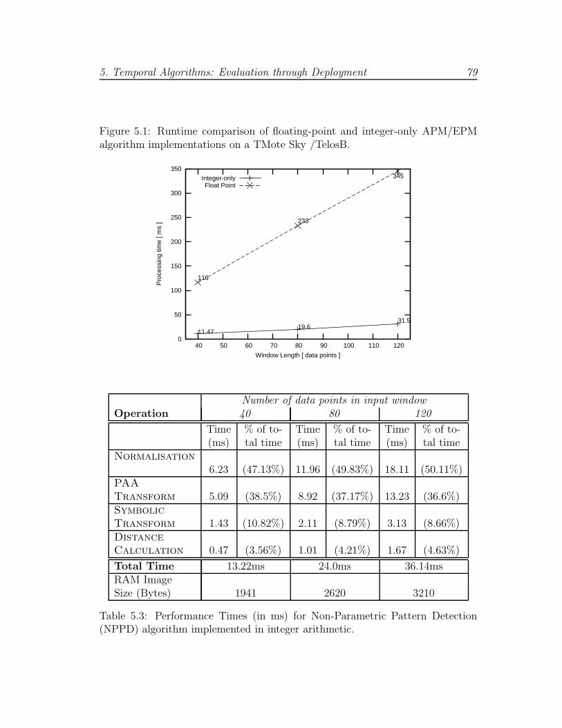
5. Temporal Algorithms: Evaluation through Deployment 79
Figure 5.1: Runtime comparison of floating-point and integer-only APM/EPMalgorithm implementations on a TMote Sky /TelosB.
0
50
100
150
200
250
300
350
40 50 60 70 80 90 100 110 120
Pro
cess
ing
time
[ ms
]
Window Length [ data points ]
11.47
116
19.6
233
31.5
345Integer-onlyFloat Point
Number of data points in input windowOperation 40 80 120
Time % of to- Time % of to- Time % of to-(ms) tal time (ms) tal time (ms) tal time
Normalisation
6.23 (47.13%) 11.96 (49.83%) 18.11 (50.11%)PAA
Transform 5.09 (38.5%) 8.92 (37.17%) 13.23 (36.6%)Symbolic
Transform 1.43 (10.82%) 2.11 (8.79%) 3.13 (8.66%)Distance
Calculation 0.47 (3.56%) 1.01 (4.21%) 1.67 (4.63%)
Total Time 13.22ms 24.0ms 36.14msRAM ImageSize (Bytes) 1941 2620 3210
Table 5.3: Performance Times (in ms) for Non-Parametric Pattern Detection(NPPD) algorithm implemented in integer arithmetic.
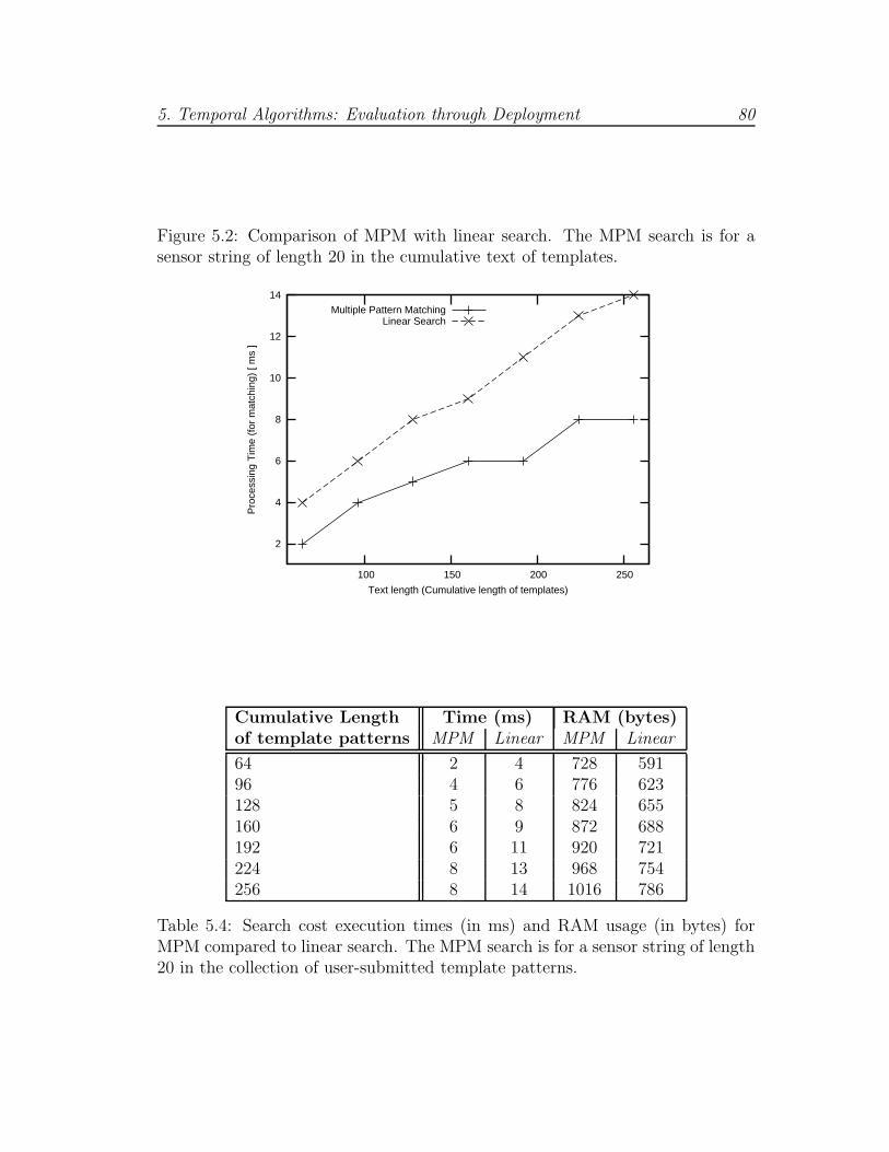
5. Temporal Algorithms: Evaluation through Deployment 80
Figure 5.2: Comparison of MPM with linear search. The MPM search is for asensor string of length 20 in the cumulative text of templates.
2
4
6
8
10
12
14
100 150 200 250
Pro
cess
ing
Tim
e (f
or m
atch
ing)
[ m
s ]
Text length (Cumulative length of templates)
Multiple Pattern MatchingLinear Search
Cumulative Length Time (ms) RAM (bytes)of template patterns MPM Linear MPM Linear
64 2 4 728 59196 4 6 776 623128 5 8 824 655160 6 9 872 688192 6 11 920 721224 8 13 968 754256 8 14 1016 786
Table 5.4: Search cost execution times (in ms) and RAM usage (in bytes) forMPM compared to linear search. The MPM search is for a sensor string of length20 in the collection of user-submitted template patterns.
5. Temporal Algorithms: Evaluation through Deployment 81
5.2 Dynamic Sampling Frequency Management
(DSFM) Algorithm
Dynamic Sampling Frequency Management (DSFM) extends Non-Parametric
Pattern Detection (NPPD) by allowing WSN nodes to automatically adjust their
sampling frequency according to the rate of change of the monitored object. The
aim of DSFM is to reduce resource expenditure attributed to MCU and sensor
acquisition during periods of relative stability of the monitored object.
The procedural steps for DSFM are listed in Algorithm 5.1 and are similar to
Non-Parametric Pattern Detection (cf. Section 3.4) involving an identical learn-
ing phase. When learning completes, a node progressively reduces its sampling
frequency until the minimum allowed sampling frequency is achieved. If a node
observes a distance greater than the maximum distance learnt caused by a pattern
classified as unusual, the maximum allowed sampling frequency is restored.
We recognise that certain WSN applications have strict sampling frequency
requirements dictated by signal periodicity. If these requirements can be specified
as a sampling frequency interval, DSFM selects and adjusts sampling frequency
within the interval relaxing the need for pre-deployment signal analysis.

5. Temporal Algorithms: Evaluation through Deployment 82
Algorithm 5.1 Dynamic Sampling Frequency Management (DSFM) Algorithm
Require: learnPeriod 6= εRequire: min-sampling-frequency, max-sampling-frequency
1: maxδ, learnCounter← 02: while learnCounter ≤ learnPeriod do3: ut ← int sax(sensor-valuest[])
{sensor-valuest is a window with the most recent observations}4: ut−1 ← int sax(sensor-valuest−1[])
{sensor-valuest−1 is a window temporally shifted by one time unit}5: δ ← ‖ut − ut−1‖6: if δ > maxδ then7: maxδ ← δ8: end if9: Increment learnCounter by 110: end while11: loop12: ut ← int sax(sensor-valuest[])13: ut−1 ← int sax(sensor-valuest−1[])14: δ ← ‖ut − ut−1‖15: if δ ≥ maxδ then16: Call Notify17: if sampling-frequency < max-sampling-frequency then18: sampling-frequency ← max-sampling-frequency
{Set sampling frequency to maximum allowed}19: end if20: else21: if sampling-frequency > min-sampling-frequency then22: if sampling-frequency ×.9 > min-sampling-frequency then23: sampling-frequency ← sampling-frequency ×.9
{Reduce sampling frequency by 10%}24: else25: sampling-frequency ← min-sampling-frequency
26: end if27: end if28: end if29: end loop

5. Temporal Algorithms: Evaluation through Deployment 83
5.2.1 Data Centre WSN Deployment
To assess the operation of Dynamic Sampling Frequency Management (DSFM),
we deploy the algorithm on a network of seven TMote Sky/TelosB nodes in a
commercial data centre.
Context and Deployment Details
The deployment was commissioned by a global telecommunications company as
a proof of concept for a data centre monitoring solution. It was carried out at
the company’s London headquarters in a data centre hosting over 200 servers and
associated storage and networking equipment.
The most common type of failures observed by this company are due to cooling
problems that cause, sometimes unrecoverable, hardware failures. These cooling
failures are usually attended by a dedicated team of four facilities employees.
A Building Management System (BMS) with wired sensors is responsible for
detecting increases in temperature and notifying the facilities team. However,
in the last two years technical employees noticed a large number of BMS false
negatives where sustained high temperature events were not identified. A number
of servers equipped with built-in sensors and management agents periodically
alert on high inlet or ambient temperature observations without a corresponding
alert from the BMS.
On the 2nd of May 2010, the company experienced a substantial failure of
one of the two air conditioning units in its London data centre. The failure re-
duced the cooling capacity to half and caused concern for critical systems hosted
in the data centre. The facilities team investigated the problem and found that
the failed cooling unit was in need of complete replacement. While waiting for
the purchase, delivery and replacement of the faulty unit, the facilities team
decided to temporarily reduce rising temperatures by opening windows, to facil-
itate cold air circulation, and deploying several portable air-conditioning units.
In hindsight, the open windows adversely affected the operation of computing
equipment and caused latent failures, due to dust particles gathering on air ducts
5. Temporal Algorithms: Evaluation through Deployment 84
of sensitive hardware.
Metric
In order to assess the benefit of the DSFM algorithm the metric of MCU work-
load saving is introduced as the number of timer ticks saved due to DSFM in
comparison with operating under constant sampling frequency.
Hypothesis
The DSFM algorithm can reduce MCU workload, expressed as total number of
timer ticks, by autonomously adjusting node sampling frequency without com-
promising detection of pattern events.
Experiments
During the time of the cooling failure, we were asked to deploy a WSN for a
week with an application objective of alerting upon any significant and sustained
changes in temperature or humidity. This offered us the opportunity to validate
the operation of DSFM.
The floor plan and deployed nodes are shown in Figure 5.3 with the circled
numbers representing node IDs and locations. Nodes 1, 3 and 4 were located
on top of equipment racks at a height of 215cm, nodes 5 and 6 were placed on
the middle of racks at approximate height of 110cm and nodes 2 and 7 were
placed on workbench surfaces at a height of 105cm. Node 1 is the base station,
running the TinyOS BaseStation utility, and the only node powered by a USB/
serial connection to a computer, with the latter used to log notification packets
received from nodes 2 − 7 via node 1. Instead of running DSFM, it passively
collects temperature and relative humidity at a constant frequency of 0.5Hz.
Nodes 2−7 run the DSFM algorithm and employ an alphabet of 10 characters
for pattern detection and a compression ratio of 2/1. DSFM requires a sampling
frequency interval with minimum and maximum sampling frequencies acceptable
by the user. The interval is specified as [0.5, 0.125]Hz (or [2048, 8192] sampling
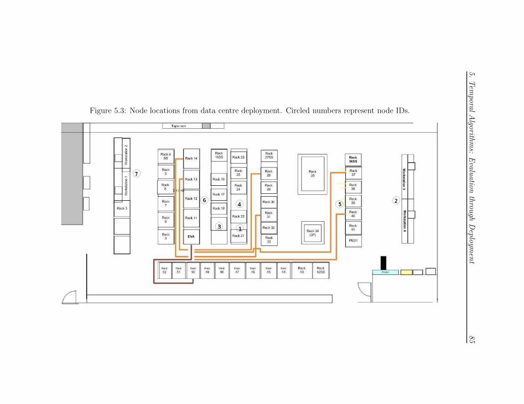
5.Tem
poralAlgo
rithms:
Evaluatio
nthrough
Deploym
ent
85
Figure 5.3: Node locations from data centre deployment. Circled numbers represent node IDs.
5. Temporal Algorithms: Evaluation through Deployment 86
period using TinyOS Timers’ binary milliseconds [STG07]). WSN nodes were
tasked with different symbolic input window lengths, specifically: 128 data points
for nodes 3 and 6, 256 data points for nodes 4 and 5 and 512 data points for nodes
2 and 7.
Nodes 2−7 initiate learning the normal rate of change by monitoring distances
between temporally adjacent strings as described in Section 3.4. Learning dura-
tion was set to the first day of deployment or (approximately) 43, 200 timer ticks.
When learning completes, nodes let DSFM manage the sampling frequency using
the TinyOS stop and startPeriodic timer commands. There are two separate
independent timers for each monitored attribute (temperature and humidity).
Whenever DSFM adjusts the frequency, it sends a packet to the base station to
notify the relative time of adjustment (in timer ticks), the string distance caus-
ing the adjustment, the name of the timer monitored attribute and old and new
sampling frequencies. In practice, transmission is not necessary and was used for
experiment verification purposes.
During the deployment, there was one natural pattern event caused by a
thunderstorm that triggered a rise in relative humidity spanning a period of over
12 hours. Such external events do not usually impact ambient temperature and
indoor humidity, however this was not the case during the deployment since data
centre windows were ajar.
The DSFM algorithm detected two and five pattern events over relative hu-
midity and temperature attributes respectively. Except one, all patterns detected
on the relative humidity attribute were during and after the thunderstorm which
caused an approximately 7% increase of relative humidity. Nine pattern events
were triggered during the drop in relative humidity after the thunderstorm. There
was one false positive triggered by node 3. In line with the emulation results of
Section 4.2.1, the number of patterns classified as unusual reduced as the window
length increased. Although all the detected patterns refer to the same physi-
cal event that spanned several hours, the algorithms detected 22 patterns that
represent changes in the signal spanning, at most, a few minutes.
On the temperature attribute, there was a total of five pattern events, out
5. Temporal Algorithms: Evaluation through Deployment 87
of which two were false positives. Nodes with input window lengths above 128
did not report false positives, in line with expectations from results described in
Section 4.2.1. The remaining three unusual patterns coincided with increases and
sustained high observations. True and false positives were confirmed by technical
engineers of the company, and the three true temperature pattern events were
matched with notifications by the BMS3 and alerts sent from server management
agents. An example of the data, as recorded by the base station, with markers
of patterns detected by nodes 2− 7 is shown in Figure 5.4.
Findings
The main finding of this experiment is that savings in node workload attributed
to DSFM amount to 64% fewer timer ticks and related sensor data acquisition.
Taking into account that WSN nodes typically execute tasks in a constant loop
dictated by their timers, reducing the frequency of task execution can conse-
quently conserve resources.
Per-node results including the number of true and false positives reported are
shown in Table 5.5. If we use node 4 as an example, without DSFM its timers
would have fired 604, 800 times, assuming a constant sampling frequency of 0.5Hz.
With DSFM, its timers fired 216, 059 times. There was a total of 495 sampling
frequency adjustments by DSFM that were verified correct, as they would either
follow the end of the learning phase or a detected pattern event.
Overall the hypothesis that DSFM can reduce the MCU workload was con-
firmed in this deployment. The majority of reported patterns coincided with the
thunderstorm event, suggesting that pattern detection is not adversely affected
by automatic sampling frequency adjustments.
3The BMS cannot monitor relative humidity.
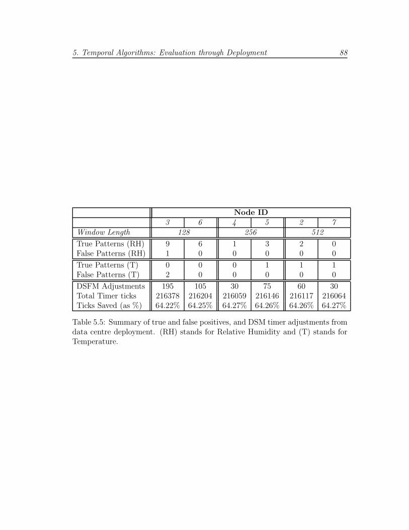
5. Temporal Algorithms: Evaluation through Deployment 88
Node ID3 6 4 5 2 7
Window Length 128 256 512
True Patterns (RH) 9 6 1 3 2 0False Patterns (RH) 1 0 0 0 0 0
True Patterns (T) 0 0 0 1 1 1False Patterns (T) 2 0 0 0 0 0
DSFM Adjustments 195 105 30 75 60 30Total Timer ticks 216378 216204 216059 216146 216117 216064Ticks Saved (as %) 64.22% 64.25% 64.27% 64.26% 64.26% 64.27%
Table 5.5: Summary of true and false positives, and DSM timer adjustments fromdata centre deployment. (RH) stands for Relative Humidity and (T) stands forTemperature.
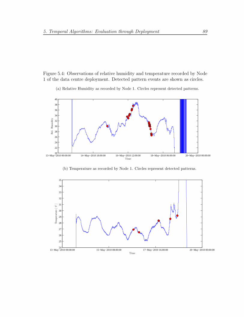
5. Temporal Algorithms: Evaluation through Deployment 89
Figure 5.4: Observations of relative humidity and temperature recorded by Node1 of the data centre deployment. Detected pattern events are shown as circles.
(a) Relative Humidity as recorded by Node 1. Circles represent detected patterns.
13−May−2010 00:00:00 14−May−2010 18:00:00 16−May−2010 12:00:00 18−May−2010 06:00:00 20−May−2010 00:00:0020
22
24
26
28
30
32
34
36
38
40
Time
Rel
.H
um
idit
y
(b) Temperature as recorded by Node 1. Circles represent detected patterns.
13−May−2010 00:00:00 15−May−2010 08:00:00 17−May−2010 16:00:00 20−May−2010 00:00:0024
25
26
27
28
29
30
31
32
33
34
35
Time
Tem
per
atu
re[C
]
5. Temporal Algorithms: Evaluation through Deployment 90
5.3 Integration with Publish/Subscribe
The proposed pattern matching and detection algorithms are accessible via a
Publish/Subscribe (Pub/Sub) interface that serves two purposes:
• It allows users to express interests in events as subscriptions [EFGK03].
• It allows nodes to notify users upon pattern event occurrences.
A subscription for a pattern of interest is disseminated in the WSN, stored by
nodes and compared against sensor produced strings according to matching oper-
ators described in Section 3.1.3. A notification is a message destined for the sub-
scriber when a pattern event is detected or matched against a template by a WSN
node. We refer the reader to the Pub/Sub literature [DGH+06, HGM04, EFGK03,
CJ02] for a detailed discussion of the Pub/Sub communication paradigm.
The pattern matching and detection algorithms are integrated with a Publish/
Subscribe (Pub/Sub) interface by extending the TinyCOPS [HHK+08] framework
which provides a content-based Pub/Sub service for WSN nodes. This integra-
tion of pattern matching and detection with Publish/Subscribe was tested in the
data centre deployment of Section 5.2.1 where the notification delivery protocol
[HHK+08] was responsible for delivering pattern event notifications from nodes
to the base station.
TinyCOPS allows additional functionality to be introduced into the framework
with Service Extension Components (SECs) without modification of the existing
Pub/Sub core. The temporal pattern matching and detection algorithms fol-
low this mechanism and provide their functionality through an Attribute Service
Extension Component (ASEC) that processes WSN observations in the manner
described in the algorithms of Chapter 3.
The pattern matching and detection algorithms employ default initialisation
values for alphabet size, compression ratio and numeric sensor window length,
however users can override these values by sending subscription metadata mes-
sages to WSN nodes. Such messages are widely used in TinyCOPS and interact
5. Temporal Algorithms: Evaluation through Deployment 91
with our algorithms via the developed ASEC. Subscription metadata is repre-
sented as attribute-value pairs, for example 〈CompRatio, 4〉 instructs one or more
nodes to set their symbolic conversion compression ratio to 4/1.
TinyCOPS employs TinyOS protocols such as Trickle [LPCS04] for dissem-
ination of subscriptions and Collection Tree Protocol (CTP) for collection of
notifications. The integration of our pattern matching and detection algorithms
through the developed ASEC with the communication mechanisms of TinyCOPS,
confirms that our algorithms are compatible with standard TinyOS protocols and
do not require any code modifications in the underlying networking layers. This
means that pattern matching and detection algorithms are agnostic of lower layer
protocols and decoupled from both the WSN naming/addressing schemes and the
choice of subscription/notification delivery protocols.
5.4 Observations from Further Deployments
In order to show that our algorithms can operate in a new class of extremely
resource constrained devices, we select the Wireless Identification and Sensing
Platform (WISP) node developed by Intel Research [Res08]. The WISP is a
node that combines the capabilities of RFID tags with those of WSN nodes.
Its distinctive feature is that it lacks on-board power supply. Instead, it harvests
power from an off-the-shelf RFID reader to operate its MSP430 MCU and sensors.
This execution environment poses the challenge of achieving a computational goal
with intermittently powered hardware resources.
To verify operation in this battery-free platform, we ported the NPPD algo-
rithm and demonstrated4 pattern detection during a 2009 Knowledge Transfer
Network (KTN) event. The demonstration [ZR09c] tasked the algorithm to clas-
sify accelerometer patterns in a system used for teaching primary education pupils
the basic laws of motion (cf. [PSFR08] for more information on the project).
We found the NPPD algorithm suited this challenging environment as it does
not require prior configuration and takes approximately 13ms to classify new
4This demonstration won the Best R&D award [ZR09e].
5. Temporal Algorithms: Evaluation through Deployment 92
patterns. The algorithm spent 10 seconds to learn normal motions from on-board
accelerometer observations and subsequently classified other motions — induced
by users shaking and moving the WISP — as unusual. For this demonstration, a
window of 80 data points was employed with a sampling frequency of 20Hz and
a compression ratio of 2/1.
To alleviate the effects of intermittent and unpredictable power resources,
we installed a supercapacitor that stores accumulated power and prolongs the
lifetime of the WISP, by up to 30 seconds, when it is not within the range of the
RFID reader.
Other past deployments include a small testbed of four nodes installed in
one of our laboratory buildings for five weeks during December 2008. Having
processed over one million temperature observations, two nodes were running
probabilistic pattern detection and the other two were running non-parametric
pattern detection with the first day of deployment used as learning period.
Nodes converted numeric sequences of 40 observations to strings using a 4/1
compression ratio and a 10 letter alphabet. Neither true nor false positives were
detected, in line with expectations as temperature observations were normal in
comparison with the first day of deployment that was used as training period.
5.5 Summary of Findings
We described practical work and findings from implementing our temporal pat-
tern matching and detection algorithms and deploying on real resource con-
strained sensor networks. We found the following:
(i) The precise implementation of pattern matching and detection algorithms
incorporating integer arithmetic and related optimisations showed a factor
of ten runtime improvement in comparison with a floating point implemen-
tation.
(ii) The Dynamic Sampling Frequency Management (DSFM) algorithm was as-
sessed in a data centre deployment where it resulted in 64% fewer timer

5. Temporal Algorithms: Evaluation through Deployment 93
ticks in comparison with constant sampling frequency. The company that
commissioned the work decided to deploy a further WSN (scheduled for
summer 2011) comprised of Zolertia Z1 [Zol10] nodes.
(iii) Integration with a Publish/Subscribe framework shows that the proposed
pattern matching and detection algorithms are compatible with standard
TinyOS communication protocols and do not require modifications of lower
networking layers.
(iv) NPPD execution profile was sufficiently low to support use in a new class
of energy harvesting nodes powered from RFID readers.
These findings provide evidence that the family of algorithms introduced in Chap-
ter 3 are well-suited to extremely resource constrained nodes since they require
minimal processing time and modest RAM for the task of pattern matching and
detection.
Chapter 6
Pattern Location Estimation in
the Spatial Domain
We introduce an algorithm that operates on the spatial domain and computes
a coarse estimate of a spatial pattern event location. We focus on a particular
type of pattern event, the dispersion of a plume from a pollutant-emitting point
source in space. In contrast to the temporal algorithms of Chapter 3 that operate
autonomously without radio communication, the spatial algorithm relies on ex-
changing information with local neighbours in order to collaboratively solve the
location estimation problem.
Section 6.1 provides a more detailed description of the problem and Section
6.2 reviews the Kalman filter which forms the statistical foundation for the solu-
tion. The proposed algorithm, presented in Section 6.3, introduces a geometric
computation which is combined with the Kalman filter to estimate the location
and intensity of the source.
6.1 The Location Estimation Problem
As sensor technologies mature, costs are reduced and wireless connectivity be-
comes ubiquitous, it is possible to have dense in-situ networks of sensor nodes
in urban centres for people protection from terrorists detonating “dirty bombs”
94
6. Pattern Location Estimation in the Spatial Domain 95
[CYR+08]. WSN nodes can sense the presence of pollutants in the atmosphere
and collaborate to estimate the location, intensity and type of threat. Notifica-
tions can be sent to emergency personnel that use the information to evacuate
citizens from the affected area and neutralise the threat to the general public.
The focus of this chapter is the problem of estimating the location and inten-
sity of the “dirty bomb” inside the network. This is an instance of the Inverse
Problem [ATB05] where dispersion parameters must be estimated from sensor-
observed data.
Specifically, the problem is characterised by the following parameters: a sin-
gle static point source emits a pollutant of chemical or radiological nature. The
source is located at the unknown coordinates (xs, ys) in two dimensional space.
The presence and intensity of the pollutant in the atmosphere is sensed by N sen-
sor nodes located at (xi, yi) coordinates with i = 1, 2, . . . , N . The problem is the
distributed, collaborative and iterative estimation of the pollutant source coordi-
nates (xs, ys) and intensity I from zi sensor observations collected at coordinates
(xi, yi).
Coarse-grained estimation is chosen on the basis that it requires lower resource
consumption [Kri05], at the expense of reduced estimate accuracy, in comparison
with fine-grained approaches such as Time Difference of Arrival (TDOA) that
usually rely on strict time synchronisation. We limit the scope to an in-network
solution, in order to avoid the high energy costs associated with transmitting
observations across multihop paths to far located sinks [WDWS10, FCG10, ZG09,
GJV+05].
6.2 Kalman Filter Properties
The foundation for the pattern location estimation algorithm of this chapter is a
Kalman Filter which is an optimal estimator of the true state of a dynamic linear
system whose observations may be corrupted by noise [Sim06].
The operation of a Kalman filter is based on a Predict-Correct cycle shown
in Figure 6.1. In its simplest form, it incorporates five equations, with the first
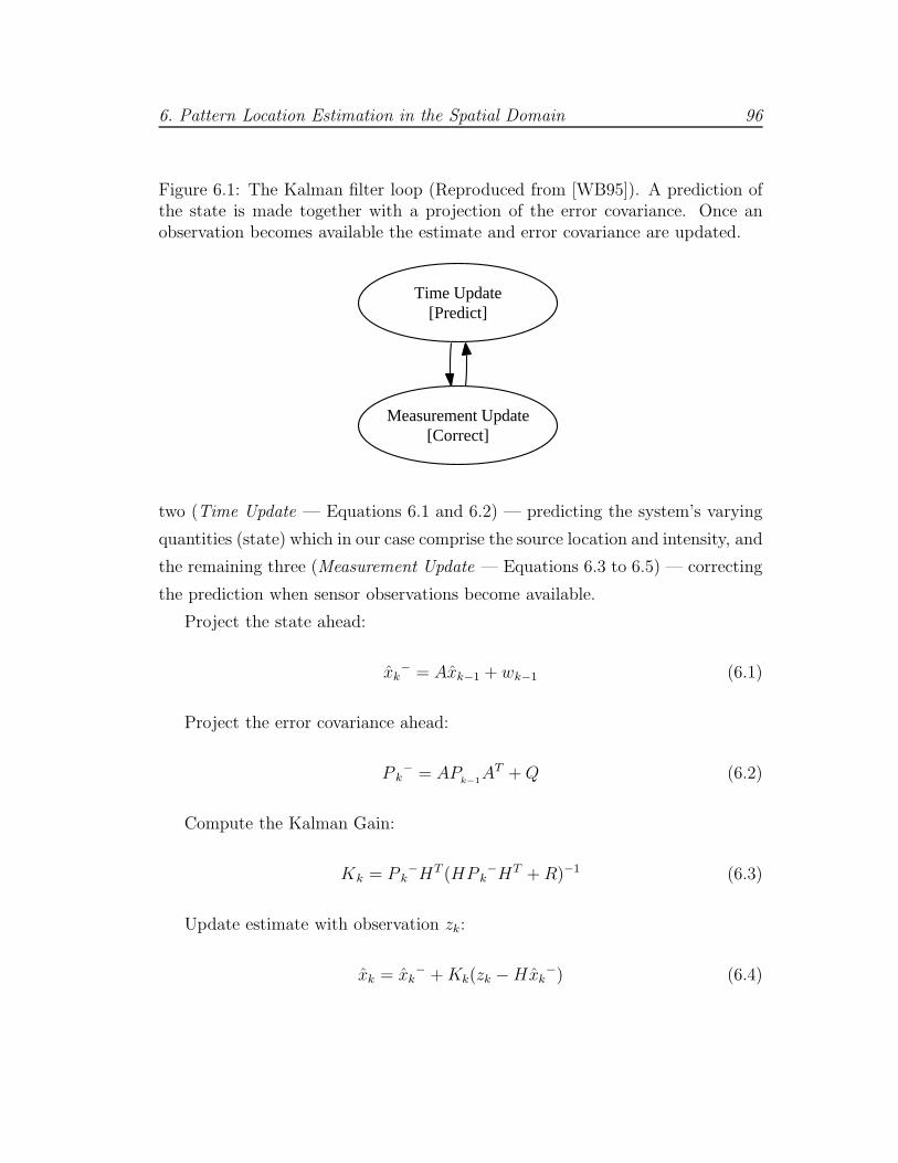
6. Pattern Location Estimation in the Spatial Domain 96
Figure 6.1: The Kalman filter loop (Reproduced from [WB95]). A prediction ofthe state is made together with a projection of the error covariance. Once anobservation becomes available the estimate and error covariance are updated.
Time Update[Predict]
Measurement Update[Correct]
two (Time Update — Equations 6.1 and 6.2) — predicting the system’s varying
quantities (state) which in our case comprise the source location and intensity, and
the remaining three (Measurement Update — Equations 6.3 to 6.5) — correcting
the prediction when sensor observations become available.
Project the state ahead:
xk− = Axk−1 + wk−1 (6.1)
Project the error covariance ahead:
P k− = AP
k−1AT +Q (6.2)
Compute the Kalman Gain:
Kk = P k−HT (HP k
−HT +R)−1 (6.3)
Update estimate with observation zk:
xk = xk− +Kk(zk −Hxk
−) (6.4)

6. Pattern Location Estimation in the Spatial Domain 97
Update the error covariance:
Pk = (I −KkH)P k− (6.5)
Where:
xk− is the a priori state estimate.
xk is the a posteriori state estimate.
A is the state transition matrix.
w is the white, zero-mean, uncorrelated noise.
P k− is the a priori error covariance.
P k is the a posteriori error covariance.
Q is the process covariance.
R is the observation (measurement) noise covariance.
H is the observation (measurement) matrix.
zk is the observation taken at time k.
K is the Kalman Gain.
The goal of the Kalman filter is to formulate an a posteriori estimate xk
as a linear combination of an a priori estimate xk− and a weighted difference
between an actual observation zk and a predicted observation Hxk−, as shown in
Equation 6.4 [WB95]. The optimal nature of the filter stems from the fact that
as the observation noise covariance R approaches zero the matrix (or scalar) K
weighs the innovation (the term (zk −Hxk−) — also referred to as the residual
or the error) more heavily. Conversely, as the a priori estimate error covariance
P k− approaches zero, the gain K weighs the residual less heavily.
The Kalman filter has several advantages that make it a suitable estimator
for our context:
• It is an optimal estimator, under the least square errors criterion.
• It is designed to tolerate measurement noise and process errors, both com-
mon properties of chemical and radiological sensors [CYR+08].
• There exist efficient integer-only implementations from the DSP community
[TK88] that can be adapted for WSN nodes.
6. Pattern Location Estimation in the Spatial Domain 98
Lastly, the Kalman filter operates in a recursive manner suitable for in-network
implementation since it only requires the last estimate instead of the entire esti-
mate history to produce the next estimate.
6.3 Spatial Pattern Location Estimation (SPLE)
Algorithm
Assuming a WSN deployed in an urban area, the estimation process initiates
independently at nodes that detect the presence of pollutant in the atmosphere
using the algorithms of Chapter 3. To avoid congestion effects from having all the
nodes in a WSN transmitting simultaneously upon detection, we assume that the
WSN is clustered with an approach such as LEACH [HCB02] or HEED [YF04].
Nodes that are assigned the role of cluster head at detection time initiate the
estimation process.
An initiating node that detects the event, estimates the state of the pattern
event as it would be observed by the neighbours of its immediate vicinity (line 2,
Algorithm 6.1). This estimate is a linear transformation of the local observation
(Equation 6.1). Next, the node tasks its nearest unvisited neighbours to report
their observations (line 4). This is shown in Figure 6.2a and is achieved by a local
broadcast. At each information exchange, the objective of the sender node is to
select a receiver located closer to the source than itself.
Neighbours receiving the message, take a current observation of the gas con-
centration and transmit is as a response to the initiating node. This is shown
in Figure 6.2b. For each response received, the Kalman filter innovation Zn =
(zk(i) − Hxk
−) is calculated (lines 5-7). Note that x is the estimate of the ini-
tiating node and each observation zk(i) has a superscript i to indicate which
neighbour reported it. The initiating node calculates the minimum innova-
tion argminz
(zk(i) − Hxk
−) and selects the neighbour i who reported the error-
minimising observation as the next hop (line 8). This is shown in Figure 6.2c.
During node selection, the selecting node changes its state to visited and
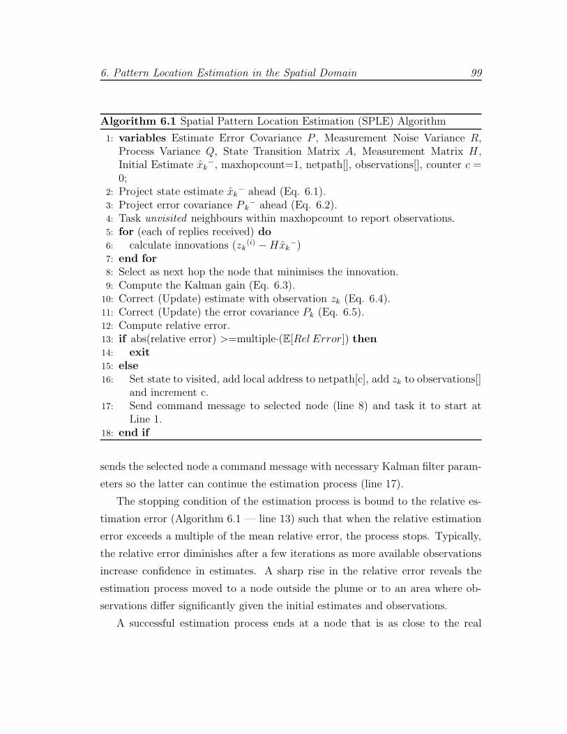
6. Pattern Location Estimation in the Spatial Domain 99
Algorithm 6.1 Spatial Pattern Location Estimation (SPLE) Algorithm
1: variables Estimate Error Covariance P , Measurement Noise Variance R,Process Variance Q, State Transition Matrix A, Measurement Matrix H ,Initial Estimate xk
−, maxhopcount=1, netpath[], observations[], counter c =0;
2: Project state estimate xk− ahead (Eq. 6.1).
3: Project error covariance P k− ahead (Eq. 6.2).
4: Task unvisited neighbours within maxhopcount to report observations.5: for (each of replies received) do6: calculate innovations (zk
(i) −Hxk−)
7: end for8: Select as next hop the node that minimises the innovation.9: Compute the Kalman gain (Eq. 6.3).10: Correct (Update) estimate with observation zk (Eq. 6.4).11: Correct (Update) the error covariance Pk (Eq. 6.5).12: Compute relative error.13: if abs(relative error) >=multiple·(E[Rel Error]) then14: exit15: else16: Set state to visited, add local address to netpath[c], add zk to observations[]
and increment c.17: Send command message to selected node (line 8) and task it to start at
Line 1.18: end if
sends the selected node a command message with necessary Kalman filter param-
eters so the latter can continue the estimation process (line 17).
The stopping condition of the estimation process is bound to the relative es-
timation error (Algorithm 6.1 — line 13) such that when the relative estimation
error exceeds a multiple of the mean relative error, the process stops. Typically,
the relative error diminishes after a few iterations as more available observations
increase confidence in estimates. A sharp rise in the relative error reveals the
estimation process moved to a node outside the plume or to an area where ob-
servations differ significantly given the initial estimates and observations.
A successful estimation process ends at a node that is as close to the real

6. Pattern Location Estimation in the Spatial Domain 100
pollutant source as possible. The coordinates and observation of that node, be-
come the final estimate and are transmitted to the application user together with
the netpath and observations arrays. The former is a trajectory sequence of
coordinates that indicate the path of the estimation process and the latter is a
sequence of observations taken by nodes participating in the estimation process.
The enhance the quality of the estimates we introduce a geometric computa-
tion that operates in the following manner: at initiation of the estimation process,
the cluster heads (or initiating nodes) communicate with each other to establish
the centroid of the Convex Hull formed by their coordinates. The convex hull
is the boundary of the minimal convex set containing a finite set of points, rep-
resenting WSN nodes. This is shown in Figure 6.3a. The coordinates of the
centroid are stored for later use.
After four1 hops nodes carrying out the estimation task re-evaluate the cen-
troid of the convex hull formed by their current coordinates. By differencing
the coordinates of the previously evaluated convex hull centroid with those of
the current centroid, a quadrant direction is established. This is one of the four
Cartesian space regions in which the majority of nodes participating in the pro-
cess estimate the source location. This region becomes the consensus and is used
to directionally propagate estimates. If a node does not have neighbours in the
mean direction of movement quadrant, it aborts the estimation run. An exam-
ple of the geometric computation is shown in Figure 6.3b: the mean direction of
movement has been established as the top-right quadrant, therefore estimates are
only propagated towards that direction.
The following chapter evaluates the geometric computation and finds that
estimation accuracy of the algorithm is improved as minority errors made by
individual nodes cannot affect the overall estimation decision.
1This parameter is configurable, but we empirically found that four hops represents a goodchoice for re-evaluating the mean direction of movement.
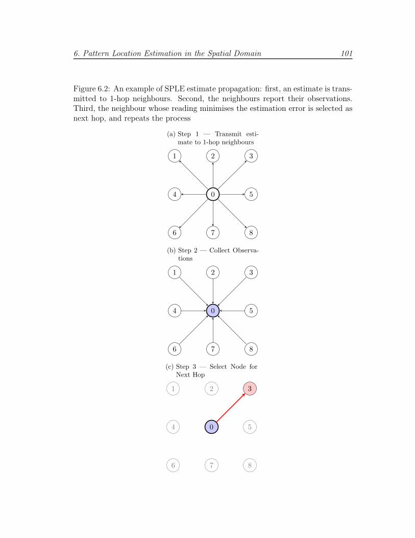
6. Pattern Location Estimation in the Spatial Domain 101
Figure 6.2: An example of SPLE estimate propagation: first, an estimate is trans-mitted to 1-hop neighbours. Second, the neighbours report their observations.Third, the neighbour whose reading minimises the estimation error is selected asnext hop, and repeats the process
(a) Step 1 — Transmit esti-mate to 1-hop neighbours
3
0 5
2
4
6 7 8
1
(b) Step 2 — Collect Observa-tions
3
0 5
2
4
6 7 8
1
(c) Step 3 — Select Node forNext Hop
3
0 5
2
4
6 7 8
1
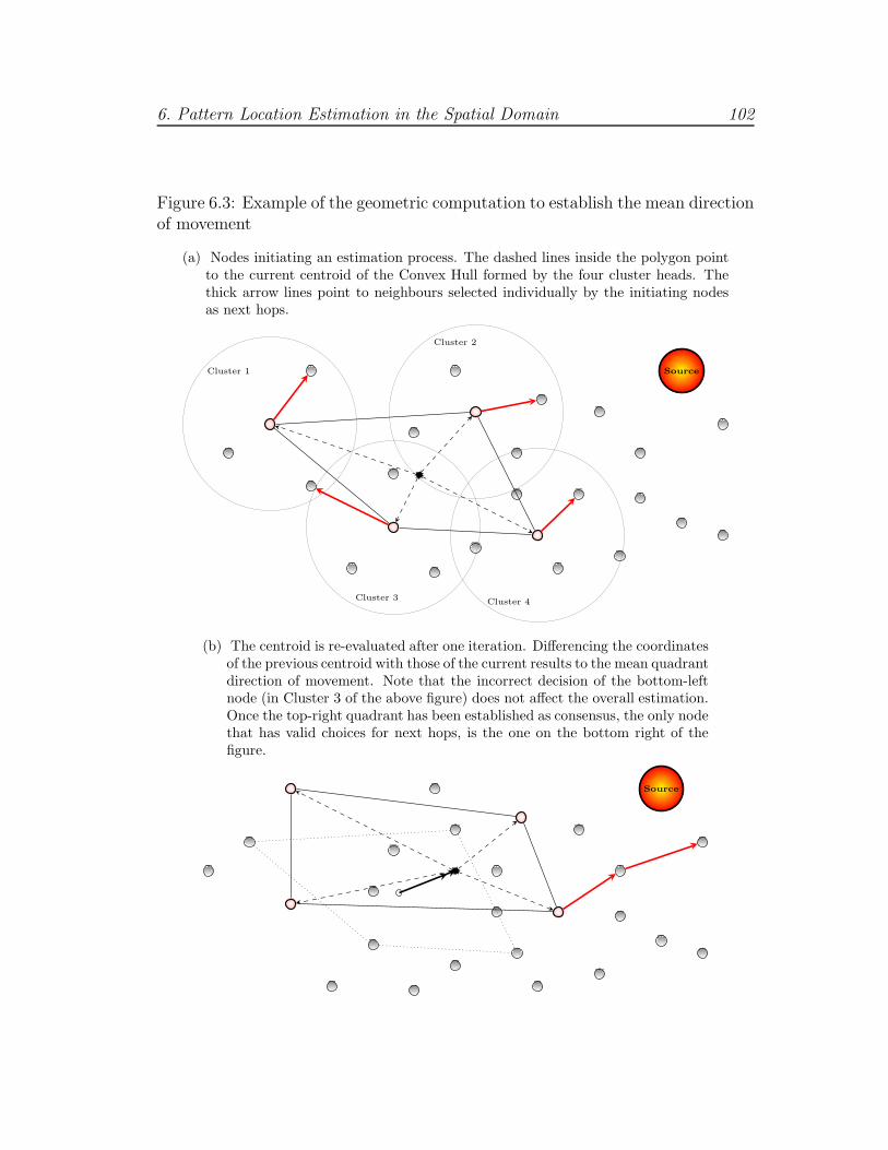
6. Pattern Location Estimation in the Spatial Domain 102
Figure 6.3: Example of the geometric computation to establish the mean directionof movement
(a) Nodes initiating an estimation process. The dashed lines inside the polygon pointto the current centroid of the Convex Hull formed by the four cluster heads. Thethick arrow lines point to neighbours selected individually by the initiating nodesas next hops.
SourceCluster 1
Cluster 2
Cluster 3 Cluster 4
(b) The centroid is re-evaluated after one iteration. Differencing the coordinatesof the previous centroid with those of the current results to the mean quadrantdirection of movement. Note that the incorrect decision of the bottom-leftnode (in Cluster 3 of the above figure) does not affect the overall estimation.Once the top-right quadrant has been established as consensus, the only nodethat has valid choices for next hops, is the one on the bottom right of thefigure.
Source

6. Pattern Location Estimation in the Spatial Domain 103
6.4 Summary
We presented an iterative coarse-grained location estimation algorithm of a point
source emitting a pollutant plume. The algorithm operates in-the-network and
provides an alternative to techniques that rely on network-wide observation har-
vesting and offline processing. A Kalman filter supplies the optimal estimation
functionality and an in-network localised information exchange builds a collabo-
rative solution to the problem.
In addition, we described a geometric computation employed to augment the
estimation accuracy by adding a consensus or majority rule to the estimation
proceedings. The consensus assumes that a group of collaborating nodes establish
mean direction of movement in order to preclude estimation deviations made by
incorrect individual node decisions.

Chapter 7
Spatial Algorithm: Evaluation
through Simulation
The purpose of this chapter is to evaluate the estimation accuracy, with respect
to varying parameters such as WSN density and node placement, of the proposed
Spatial Pattern Location Estimation (SPLE) algorithm through simulation.
Section 7.1 outlines the evaluation methodology and the setup of the simu-
lation environment including the gas dispersion model. The evaluation study of
Section 7.2 is categorised according to WSN topology of both grid and random
node placements. A summary of findings is presented in Section 7.3.
7.1 Methodology and Simulation Set-up
The experiments described in this chapter were conducted using a MATLAB
[Mat10] implementation of the SPLE algorithm. MATLAB is selected on the
basis that it offers an environment where the behaviour of the SPLE algorithm
can be tested and compared against a baseline algorithm in relatively large WSNs
fields of varying densities.
104
7. Spatial Algorithm: Evaluation through Simulation 105
7.1.1 Maximum Selection Algorithm
In order to compare the estimation accuracy of SPLE against a competitive
approach, we use the Maximum Selection algorithm. The choice of this algo-
rithm as a baseline for comparison was made on the basis of its application
[HMG03, SLV93] in contexts similar to ours and its relative simplicity. It is in-
spired from the biological approach chemotaxis [ZSST04, Ate96] where animals
and insects iteratively locate odours by moving to spatial regions where their
receptors sense a higher intensity odour than their previous position.
Similar to SPLE, the maximum selection algorithm is iterative and operates in
the following manner: the estimation process starts when one or more initiating
nodes sense the spatial pattern event. The assumptions made in Section 6.3
hold, in particular that WSN nodes participate in a cluster scheme with the
cluster heads initiating the estimation process. Upon sensing the spatial pattern
event using the algorithms of Chapter 3, nodes send a message to their local
neighbours tasking them to report their observations. The initiating node collects
the observations of its neighbours and selects the neighbour with the maximum
observation as the next hop, as it represents a node closer to the source. The
selected node changes its state to visited and repeats the process until it runs
out of unvisited local neighbours with higher intensity observations than itself.
The procedural steps for maximum selection are shown in Appendix D, Algo-
rithm D.1.
7.1.2 Dispersion Model
We use the gas dispersion and sensor response model proposed in [INM97] due
to the similarity of the investigated problem, namely a sensing system with the
capacity to locate a gas or odour source.
The model assumes one-directional wind field, constant wind speed, homoge-
neous turbulence and single pollutant source emitting gas at a constant rate. The
dimensionality of the problem is reduced by not taking height into account and
assuming that the source is placed on the floor. The resultant gas distribution

7. Spatial Algorithm: Evaluation through Simulation 106
C0 and sensor response r0 are governed by the following two equations:
C0(x, y) = p11
dsexp[−p2(ds −∆x)] (7.1)
r0(x, y) = [1 + 0.2309C0(x, y)]−0.6705 (7.2)
where:
C0(x, y) is the time-averaged gas concentration at coordinates (x, y)
p1 is given by p1 =q
2πK
q is the gas emission rate (in g/sec)
K is the turbulent diffusion coefficient
p2 is given by p2 =U2K
U is the wind speed (in m/sec)
ds is given by ds =√
(xs − x)2 + (ys − y)2
(xs, ys) are the true coordinates of the source
∆x is given by (xs − x) cos θ + (ys − y) sin θ
θ is the angle from the x-axis to the upwind directionThe experiments of Section 7.2, use the parameter values shown in Table 7.1.
7.1.3 Kalman Filter Initial Parameters
As described in the previous chapter, the estimation functionality of the SPLE al-
gorithm is realised by the combination of a geometric computation with a Kalman
filter. The filter was optimised using the functions fminsearch [Mat08b] and
Parameter Description Value
q Gas-emission rate 45, 000K Turbulent diffusion coefficient 17.463U Wind speed 3.1θ Upwind direction angle 1(xs, ys) True source coordinates) (95, 95)
Table 7.1: Parameter values for gas dispersion model
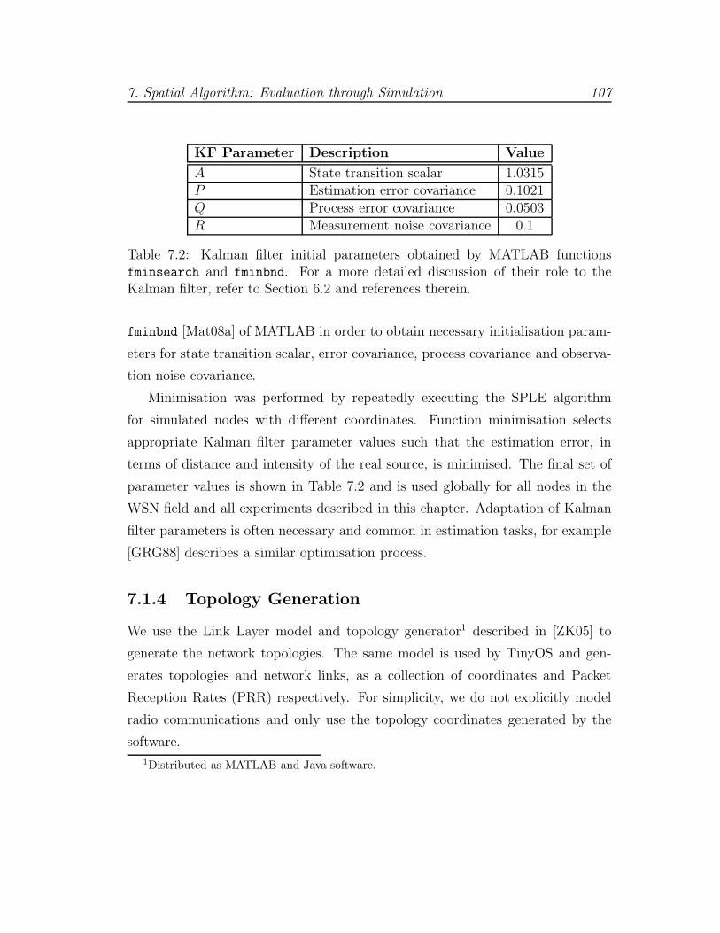
7. Spatial Algorithm: Evaluation through Simulation 107
KF Parameter Description Value
A State transition scalar 1.0315P Estimation error covariance 0.1021Q Process error covariance 0.0503R Measurement noise covariance 0.1
Table 7.2: Kalman filter initial parameters obtained by MATLAB functionsfminsearch and fminbnd. For a more detailed discussion of their role to theKalman filter, refer to Section 6.2 and references therein.
fminbnd [Mat08a] of MATLAB in order to obtain necessary initialisation param-
eters for state transition scalar, error covariance, process covariance and observa-
tion noise covariance.
Minimisation was performed by repeatedly executing the SPLE algorithm
for simulated nodes with different coordinates. Function minimisation selects
appropriate Kalman filter parameter values such that the estimation error, in
terms of distance and intensity of the real source, is minimised. The final set of
parameter values is shown in Table 7.2 and is used globally for all nodes in the
WSN field and all experiments described in this chapter. Adaptation of Kalman
filter parameters is often necessary and common in estimation tasks, for example
[GRG88] describes a similar optimisation process.
7.1.4 Topology Generation
We use the Link Layer model and topology generator1 described in [ZK05] to
generate the network topologies. The same model is used by TinyOS and gen-
erates topologies and network links, as a collection of coordinates and Packet
Reception Rates (PRR) respectively. For simplicity, we do not explicitly model
radio communications and only use the topology coordinates generated by the
software.
1Distributed as MATLAB and Java software.

7. Spatial Algorithm: Evaluation through Simulation 108
7.2 Evaluation of Spatial Pattern Location Es-
timation
For this study, we classify an estimation run as accurate if it terminates at a
WSN node located no farther than six meters from the true source. We refer to
this measure as proximity accuracy and impose the limit of six meters (Euclidean
distance) because we are targeting a coarse-grained estimation technique.
An estimation run is the estimation process of Section 6.3, from the starting
point where a node first senses the pattern event until one (or more) of its neigh-
bours, tasked with continuing the estimation process, decide to terminate because
either the terminating condition has been met or there are no more unvisited local
neighbours to continue the estimation process.
The topology terrain is a plane of 100-by-100 meters with the true source
located at coordinates (95, 95).
7.2.1 Metrics
To evaluate the estimation accuracy of SPLE, we use the following metrics:
• The Euclidean distance, in meters, between the estimated source coordi-
nates and the true source coordinates.
• The error, in relative terms, between the final intensity estimate and the
true intensity of the source.
• The length of the path, in hops, followed from beginning to end of an
estimation run.
The first two parameters determine estimation accuracy and the third parameter
offers a coarse indication of communication cost and detection latency.
7.2.2 Grid Topology
To conduct an initial investigation on the impact of WSN density to the perfor-
mance of the SPLE algorithm, we consider two grid topologies of 4, 900 and 1, 024
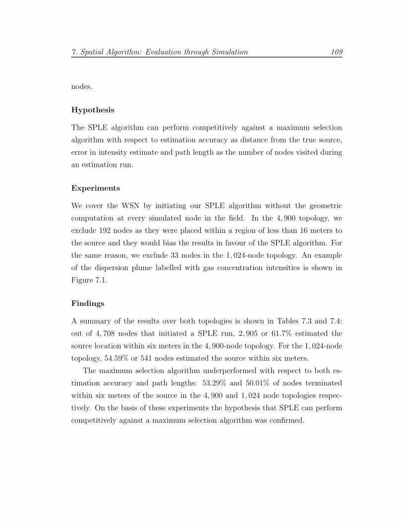
7. Spatial Algorithm: Evaluation through Simulation 109
nodes.
Hypothesis
The SPLE algorithm can perform competitively against a maximum selection
algorithm with respect to estimation accuracy as distance from the true source,
error in intensity estimate and path length as the number of nodes visited during
an estimation run.
Experiments
We cover the WSN by initiating our SPLE algorithm without the geometric
computation at every simulated node in the field. In the 4, 900 topology, we
exclude 192 nodes as they were placed within a region of less than 16 meters to
the source and they would bias the results in favour of the SPLE algorithm. For
the same reason, we exclude 33 nodes in the 1, 024-node topology. An example
of the dispersion plume labelled with gas concentration intensities is shown in
Figure 7.1.
Findings
A summary of the results over both topologies is shown in Tables 7.3 and 7.4:
out of 4, 708 nodes that initiated a SPLE run, 2, 905 or 61.7% estimated the
source location within six meters in the 4, 900-node topology. For the 1, 024-node
topology, 54.59% or 541 nodes estimated the source within six meters.
The maximum selection algorithm underperformed with respect to both es-
timation accuracy and path lengths: 53.29% and 50.01% of nodes terminated
within six meters of the source in the 4, 900 and 1, 024 node topologies respec-
tively. On the basis of these experiments the hypothesis that SPLE can perform
competitively against a maximum selection algorithm was confirmed.
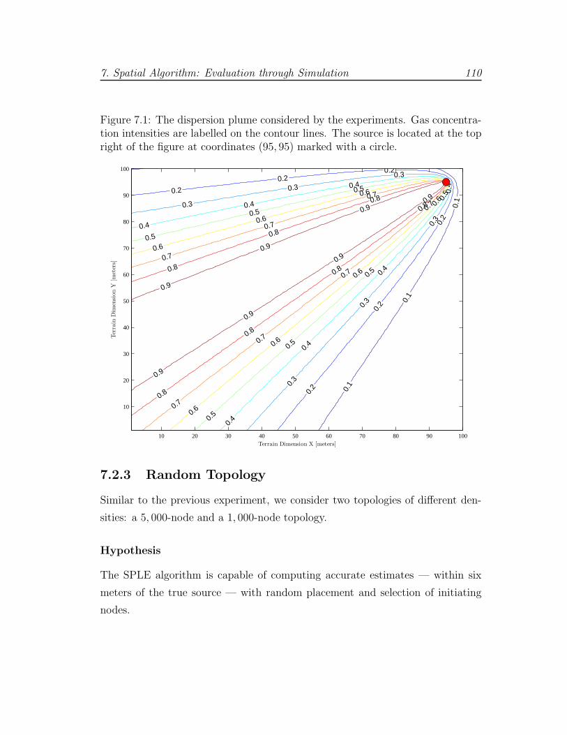
7. Spatial Algorithm: Evaluation through Simulation 110
Figure 7.1: The dispersion plume considered by the experiments. Gas concentra-tion intensities are labelled on the contour lines. The source is located at the topright of the figure at coordinates (95, 95) marked with a circle.
0.1
0.1
0.1
0.2
0.2
0.2
0.20.2
0.2
0.3
0.3
0.3
0.3
0.3
0.3
0.4
0.4
0.4
0.40.4
0.4
0.4
0.5
0.5
0.5
0.50.5
0.5
0.5
0.6
0.6
0.6
0.6
0.6
0.6
0.6
0.7
0.7
0.7
0.70.7
0.7
0.7
0.8
0.8
0.80.8
0.8
0.8
0.8
0.9
0.9
0.90.9
0.9
0.9
0.9
Terrain Dimension X [meters]
Ter
rain
Dim
ensi
on
Y[m
eter
s]
10 20 30 40 50 60 70 80 90 100
10
20
30
40
50
60
70
80
90
100
7.2.3 Random Topology
Similar to the previous experiment, we consider two topologies of different den-
sities: a 5, 000-node and a 1, 000-node topology.
Hypothesis
The SPLE algorithm is capable of computing accurate estimates — within six
meters of the true source — with random placement and selection of initiating
nodes.

7. Spatial Algorithm: Evaluation through Simulation 111
SPLE Max Selection
Proximity Accuracy(% of nodes ending an estimationrun within six meters of the source) 61.7 % 53.29 %Mean Distance 3.26 2.87Median Distance 3 3Intensity Accuracy(Mean Relative Error) 6.73 % 8.17%Mean Path Length (hops) 72.16 77.01Median Path Length (hops) 74 79
Table 7.3: Baseline comparison of our SPLE algorithm with the Maximum Se-lection algorithm over 4, 900-node grid topology. 4, 708 WSN nodes initiate theestimation run and their results are summarised.
Experiments
We assume a WSN that arranges nodes in clusters using a method like LEACH
[HCB02] or HEED [YF04]. As described in Section 6.3, the role of a cluster head
is to initiate an estimation run and to collaborate with neighbouring cluster heads
in order to compute the geometric mean direction of movement.
Similar to the previous experiments, to avoid bias of results in favour of the
SPLE algorithm nodes placed within 16 meters of the true source are not consid-
ered as candidates for initiating an estimation run.
The experiments are divided into eight trials testing 1, 000 possible clusters
with 4 and 5 nodes per cluster.
Findings
For reference, we perform an initial evaluation of the SPLE algorithm without its
geometric computation component. The results were comparable with those of
the grid topologies: 50.74% and 46.09% of nodes computed an accurate proximity
estimate, for the 5, 000 and 1, 000 topologies respectively.
The strength of the geometric computation is demonstrated by achieving im-
proved mean proximity accuracy of 87.24% and 90.91% with four and five cluster
7. Spatial Algorithm: Evaluation through Simulation 112
SPLE Max Selection
Proximity Accuracy(% of nodes ending an estimationrun within six meters of the source) 54.59 % 50.01 %Mean Distance 4.13 3.99Median Distance 4 4Intensity Accuracy(Mean Relative Error) 9.11 % 10.33%Mean Path Length (hops) 39.52 41.91Median Path Length (hops) 38 43
Table 7.4: Baseline comparison of our SPLE algorithm with the Maximum Se-lection algorithm over 1, 024-node grid topology. 991 WSN nodes initiate theestimation run and their results are summarised.
heads participating in the geometric computation respectively. This means that
over eight trials, the geometric computation with SPLE maintained estimation
accuracy over 85%; that is over 85% of nodes were successful in estimating the
true source coordinates within six meters. In addition, mean distance to the
source and path lengths also improve with results for the 5, 000-node topology
summarised in Table 7.5.
The experiments were repeated on five 1, 000-node topologies and the results
are shown in Table 7.6. It can be seen that proximity accuracy is affected by
topology with a worst case of 86.53% of nodes successfully estimating the true
source coordinates within six meters. Results for five cluster heads participating
in the geometric computation (not shown on the table for clarity) are slightly
higher with a maximum of 98.21% of nodes successfully estimating the true source
within six meters of its actual location.
An example of the geometric computation with multiple evaluations of the
convex hull centroids is shown in Figure 7.2. Overall the hypothesis that SPLE
can compute estimates accurate within six meters of the true source location with-
out relying on particular initiating node selection or placement was confirmed.
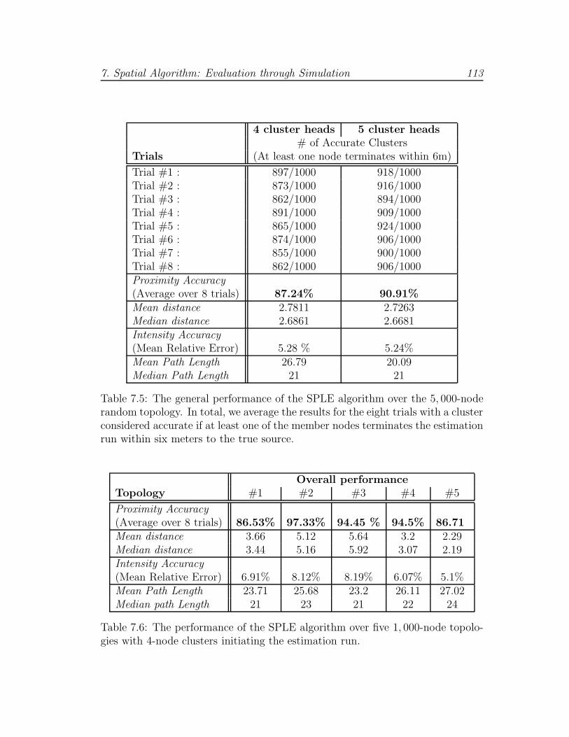
7. Spatial Algorithm: Evaluation through Simulation 113
4 cluster heads 5 cluster heads# of Accurate Clusters
Trials (At least one node terminates within 6m)
Trial #1 : 897/1000 918/1000Trial #2 : 873/1000 916/1000Trial #3 : 862/1000 894/1000Trial #4 : 891/1000 909/1000Trial #5 : 865/1000 924/1000Trial #6 : 874/1000 906/1000Trial #7 : 855/1000 900/1000Trial #8 : 862/1000 906/1000Proximity Accuracy(Average over 8 trials) 87.24% 90.91%Mean distance 2.7811 2.7263Median distance 2.6861 2.6681Intensity Accuracy(Mean Relative Error) 5.28 % 5.24%Mean Path Length 26.79 20.09Median Path Length 21 21
Table 7.5: The general performance of the SPLE algorithm over the 5, 000-noderandom topology. In total, we average the results for the eight trials with a clusterconsidered accurate if at least one of the member nodes terminates the estimationrun within six meters to the true source.
Overall performanceTopology #1 #2 #3 #4 #5
Proximity Accuracy(Average over 8 trials) 86.53% 97.33% 94.45 % 94.5% 86.71Mean distance 3.66 5.12 5.64 3.2 2.29Median distance 3.44 5.16 5.92 3.07 2.19Intensity Accuracy(Mean Relative Error) 6.91% 8.12% 8.19% 6.07% 5.1%Mean Path Length 23.71 25.68 23.2 26.11 27.02Median path Length 21 23 21 22 24
Table 7.6: The performance of the SPLE algorithm over five 1, 000-node topolo-gies with 4-node clusters initiating the estimation run.

7. Spatial Algorithm: Evaluation through Simulation 114
7.3 Summary of Findings
We conducted evaluation through simulation of the Spatial Pattern Location Esti-
mation (SPLE) algorithm. We found that, under certain assumptions, the SPLE
algorithm is accurate at the task of locating the pollutant source coordinates
within six meters. Specifically we found the following:
(i) The SPLE algorithm is competitive against a maximum selection algorithm.
The latter follows the maximum sensor observations in an attempt to locate
the pollutant source.
(ii) Four cluster heads collaborating in the geometric computation improve the
proximity accuracy of SPLE with 86%-97% of nodes estimating the source
location within six meters of its actual coordinates on the random topologies.
(iii) The overall performance of the SPLE algorithm is not significantly affected
by placement and selection of initiating nodes with a worst-case accuracy
of over 85% across the random topologies.
Finally, the study described in this chapter opens several directions for future
work further explored in Section 8.4.
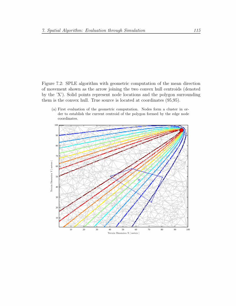
7. Spatial Algorithm: Evaluation through Simulation 115
Figure 7.2: SPLE algorithm with geometric computation of the mean directionof movement shown as the arrow joining the two convex hull centroids (denotedby the ’X’). Solid points represent node locations and the polygon surroundingthem is the convex hull. True source is located at coordinates (95,95).
(a) First evaluation of the geometric computation. Nodes form a cluster in or-der to establish the current centroid of the polygon formed by the edge nodecoordinates.
Terrain Dimension X [ meters ]
Ter
rain
Dim
ensi
on
Y[m
eter
s]
10 20 30 40 50 60 70 80 90 100
10
20
30
40
50
60
70
80
90
100
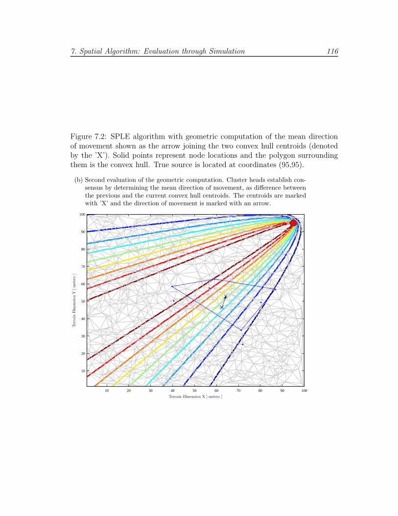
7. Spatial Algorithm: Evaluation through Simulation 116
Figure 7.2: SPLE algorithm with geometric computation of the mean directionof movement shown as the arrow joining the two convex hull centroids (denotedby the ’X’). Solid points represent node locations and the polygon surroundingthem is the convex hull. True source is located at coordinates (95,95).
(b) Second evaluation of the geometric computation. Cluster heads establish con-sensus by determining the mean direction of movement, as difference betweenthe previous and the current convex hull centroids. The centroids are markedwith ’X’ and the direction of movement is marked with an arrow.
Terrain Dimension X [ meters ]
Ter
rain
Dim
ensi
on
Y[m
eter
s]
10 20 30 40 50 60 70 80 90 100
10
20
30
40
50
60
70
80
90
100
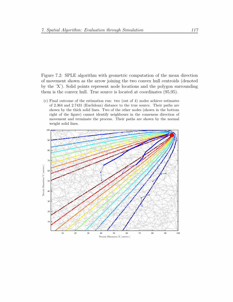
7. Spatial Algorithm: Evaluation through Simulation 117
Figure 7.2: SPLE algorithm with geometric computation of the mean directionof movement shown as the arrow joining the two convex hull centroids (denotedby the ’X’). Solid points represent node locations and the polygon surroundingthem is the convex hull. True source is located at coordinates (95,95).
(c) Final outcome of the estimation run: two (out of 4) nodes achieve estimatesof 2.364 and 2.7431 (Euclidean) distance to the true source. Their paths areshown by the thick solid lines. Two of the other nodes (shown in the bottomright of the figure) cannot identify neighbours in the consensus direction ofmovement and terminate the process. Their paths are shown by the normalweight solid lines.
Terrain Dimension X [ meters ]
Ter
rain
Dim
ensi
on
Y[m
eter
s]
10 20 30 40 50 60 70 80 90 100
10
20
30
40
50
60
70
80
90
100
Chapter 8
Conclusions and Future Work
In this thesis, we introduced methods and algorithms that provide pattern match-
ing and detection in extremely resource constrained Wireless Sensor Networks
(WSNs). Specifically, we presented temporal domain algorithms that process
streaming sensor observations to classify patterns that reveal interesting or un-
usual activity in the monitored process, phenomenon or structure (monitored
object). Moreover, we designed a spatial domain iterative algorithm, based on a
geometric computation and a Kalman filter that estimates the location of a gas
emitting source.
This final chapter, summarises the thesis in Section 8.1 and reviews the con-
tributions in Section 8.2. A critical appraisal of the thesis is presented in Section
8.3 and directions for future work are explored in Section 8.4.
8.1 Summary of the Thesis
Target Platform Constraints As discussed in Chapter 1, this thesis intro-
duces methods and algorithms that target extremely resource constrained WSN
nodes. A characteristic of such devices is that they are limited in power resources
and computational capabilities. In particular, Section 1.1.1 identified the high
power draw of radio in relation to other components in agreement with the view
[ZG09, MGH09, TE07, CES04, GKW+02] that locally processing sensor data to
118

8. Conclusions and Future Work 119
determine the presence of interesting or unusual activity can reduce the number
of unnecessary transmissions and, as a consequence, prolong node lifetime.
Problem Formulation The problem investigated is the provision of compu-
tationally efficient in-network pattern matching and detection algorithms that
involve solely local processing for temporal patterns and localised communica-
tion for location estimation of spatial patterns.
A pattern was defined as an ordered list of potentially non-unique sensor
observations revealing interesting or unusual activity in the monitored object.
Interesting and unusual are class labels [CBK09] defined in terms of distance,
probability or string searching.
Rationale Motivation for selecting this problem was twofold: first, pattern
matching and detection can benefit a number of reactive applications from differ-
ent domains reviewed in Chapter 2. Second, after examining related literature,
we found a number of approaches either lacked evidence of implementation for
resource constrained WSNs or assumed an out-of-network processing model that
relies on radio communication for transmitting observations to base stations.
Temporal domain patterns Chapter 3 introduced temporal domain pattern
matching and detection algorithms. The basis for the algorithms is symbolic
aggregate approximation (SAX [LKLC03]) that converts windows of streaming
sensor observations to strings. Pattern matching is performed by computing the
distance between a sensor produced pattern (sensor string) with a user submitted
template pattern (template), or by determining whether the sensor string appears
in the collection of templates. Non-parametric detection compares two temporally
adjacent sensor strings to a maximum learnt distance and probabilistic detection
computes the path probability of a sensor string, given learning data.
Evaluation was conducted in two parts: the first part (Chapter 4) emulated
the timer, sensor and ADC components of a node to simulate sensor data acqui-
sition. Experiments investigated the impact of symbolic conversion parameters
8. Conclusions and Future Work 120
— such as alphabet size, window length and compression ratio — to false posi-
tives. Further experiments compared Non-Parametric Pattern Detection against
two alternative event detection techniques. Findings confirmed that our approach
was competitive with 92.7% sensitivity (cf. Section 4.3.1). In addition, findings
from a preliminary study into the effects of measurement noise were encouraging:
detection accuracy degraded gracefully in relationship to increasing signal noise
(cf. Section 4.3.2).
The second part (Chapter 5) of evaluation validated the operational profile
of the algorithms through deployments and full implementation. The algorithms
were refactored to ensure computationally efficient pattern matching and detec-
tion runtime (cf. Section 5.1). The runtime cost is known at compile-time and
depends only on the window length of sensor observations. To achieve a re-
duction of MCU active time, an algorithm that automatically adjusts sampling
frequency according to the perceived activity level of the monitored object was
introduced (cf. Section 5.2). For validation, a WSN was deployed in a data centre
and findings showed that both automatic sampling frequency management and
non-parametric detection are feasible (cf. Section 5.2.1).
The temporal algorithms are made available to users of a reactive system
via a Publish/Subscribe (Pub/Sub) interface. Integration with Pub/Sub through
implementation (cf. Section 5.3) shows that the proposed methods and algo-
rithms are compatible with standard TinyOS communication protocols and do
not require modifications in the underlying networking layers.
Spatial Domain Patterns Spatial patterns are events with position and direc-
tion in physical space. Chapter 6 introduces a localised communication algorithm
that combines a geometric computation with a Kalman filter to solve the problem
of estimating the location and intensity of a pollutant emitting source. The mo-
tivating scenario is urban deployment of WSNs for in-network detection of dirty
bombs as an alternative to transmitting observations across multihop paths to
base stations.
Initial evaluation of the spatial pattern location estimation algorithm, shows

8. Conclusions and Future Work 121
it is competitive (cf. Section 7.2.2) compared to a maximum selection algorithm.
Furthermore, evaluation of estimation performance on a number of random WSN
topologies provides evidence that the collaborative geometric computation com-
ponent of the algorithm improves location estimation accuracy (cf. Section 7.2.3).
8.2 Summary of Contributions
This thesis makes the following contributions:
(i) Introduces five temporal domain in-network pattern matching and detection
algorithms (Chapter 3).
(ii) Provides evidence (Chapter 4) that the algorithms produce consistent results
across three case studies and are competitive against other pattern event
detection methods.
(iii) Demonstrates suitability for extremely resource constrained WSN nodes by
verifying the modest runtime requirements through implementation (Chap-
ter 5).
(iv) Introduces a geometric computation combined with a Kalman filter into a
collaborative algorithm (Chapter 6) that iteratively estimates the location
of a spatial pattern event inside-the-network.
(v) Provides evidence (Chapter 7) that the spatial algorithm is competitive
against a maximum selection approach without relying on node placement.
Overall, we believe our findings contribute towards WSN-related research in the
field of reactive systems by proposing computationally efficient algorithms for
in-network pattern matching and detection.

8. Conclusions and Future Work 122
8.3 Critical Appraisal
Despite the findings from evaluation of the proposed algorithms through deploy-
ments and simulation, further work is required to establish their general appli-
cability and competitiveness with other approaches across a number of domains.
There are several directions for improving the findings and extending the work,
explored in the next section.
8.4 Directions for Future Research
Temporal Algorithms In order to demonstrate that the algorithms can gen-
eralise beyond the range of domains already tested, that are resilient to signal
noise and competitive against a number of other event detection approaches, we
propose the following actions:
(i) Conduct a comparative evaluation of all five temporal algorithms of Chapter
3 against additional competitive techniques on a range of data sets with
varying characteristics.
(ii) Investigate the noise model of different hardware sensors and extend the
preliminary study of Section 4.3.2 with respect to accuracy of temporal
domain algorithms under varying magnitudes and types of noise.
(iii) Perform a matching and detection accuracy comparison between the pro-
posed algorithms and a straightforward thresholding technique. The latter
will require adaptation to data sets and specification of threshold values and
predicates, nevertheless shortcomings of such a technique can be quantified,
for instance with an investigation into the effect of outliers on false positives.
(iv) Compare the execution profile of the proposed algorithms to competitive
techniques and evaluate the runtime of the probabilistic pattern detection
algorithm.

8. Conclusions and Future Work 123
(v) Conduct a study into the effects of dynamic sampling frequency manage-
ment (Section 5.2) with respect to false negatives that may occur as a side
effect of reduced sensor data acquisition frequency.
Spatial Algorithm The plume dispersion scenario of Chapter 6 makes a num-
ber of simplifying assumptions to study and understand the problem parameters,
common with related research by others [GRG88, INM97, CYR+08]. To address
properties of the real world problem and extend evaluation of the proposed solu-
tion, the following directions can be pursued:
(vi) Alter the gas dispersion model assumptions and investigate the performance
of the algorithm with respect to multiple sources, variations in wind speed
and atmospheric turbulence and irregular topologies with sparse or discon-
nected regions.
(vii) Evaluate against competitive techniques such as TDOA and comparatively
investigate the communication cost and estimation latency of the algorithm.
(viii) Implement the proposed spatial algorithm for resource constrained WSN
nodes and conduct a processing measurement evaluation to verify execution
efficiency. Moreover, consider and evaluate the operational cost of a range of
filters to cater for different situations. Runtime cost analysis will contribute
towards operational predictability of the spatial algorithm.
Additional opportunities Further to the above directions that extend the
findings of this thesis in the short term, we aim to explore the following longer
term issues:
(ix) Extension of pattern matching and detection to automated diagnosis sys-
tems. In the past, we conducted data analysis from breath samples of cystic
fibrosis patients collected using a Cyranose 320 [Det07] electronic nose com-
prising an array of 32 sensors, each one responding to a particular gas. The
objective was to aid diagnosis of bacterial lung infections using samples from
8. Conclusions and Future Work 124
the electronic nose. Although the device is accompanied by classification
algorithms such as PCA and nearest neighbour, other classification algo-
rithms can be applied in vertical applications designed with a particular
objective. Research in the use of the electronic nose for classification (cf.
[DD06, SMD+04, ATH03]), indicates this is an application area where the
algorithms of Chapter 3 can apply.
(x) Development of an integer-only library comprising functions defined in the
math.h C header specification [KR78], such as sqrt, sin, cos, tan. A
software library with fixed-point implementation of varying precision for
these functions can be a valuable tool to applications that perform target
tracking or data analysis. The temporal domain algorithms rely on square
root and an integer version has already been implemented, however extend-
ing the implementation to functions outside the scope of this thesis can
benefit practitioners in the wider WSN community.
(xi) Continue to adapt the algorithms to devices with intermittent power such
as the battery-free Intel WISP [Res08] that has been used as a target plat-
form for deployment (cf. Section 5.4). A related platform [Alb08], combines
RFID tags with chemically or biologically sensitive films capable of detect-
ing chemical vapours in scenarios similar to the one considered by spatial
pattern location estimation. These devices introduce a new paradigm where
computation is intermittent and dictated by the presence of power sources
such as RFID readers. Scavenged energy is usually available in short bursts
and fluctuations can cause abrupt changes in power levels, interrupting on-
going operations. We intend to investigate the possibility and associated
cost of intermittent checkpoints to save pattern matching and detection
state in case of power failures.
Overall, we will continue to pursue deployment of WSNs targeting reactive
applications since the practical work involved often uncovers issues deeply inter-
twined with the restricted functionality of nodes and extend empirical application-
level research in WSNs.

Glossary
ADC An Analog-to-Digital Converter is a hardware component responsible for
converting continuous analog signals to discrete digital numbers. It is typi-
cally found as the interfacing component between the sensors and the pro-
cessor in a wireless sensor node. 76, 119
AIS An Artificial Immune System (AIS) is a biologically inspired system that
mimics the human immune system to solve a problem. 28, 35
BMS A Building Management System (BMS) is a computer-based system that
aims to monitor a building’s mechanical and electrical equipment such as
cooling, heating, lighting and power. 83
BSN A more specific type of WSN that employs various sensors to provide con-
tinuous monitoring and analysis of physiological parameters of human sub-
jects. 26, 27
Convex Hull A Convex Hull for a set of points P in a real vector space V is
the minimal convex set containing P . It represents the boundary of the
minimal convex set containing the set of points P in the plane. 100
EWMA An Exponentially Weighted Moving Average (EWMA) is a statistical
technique used to analyse a set of data points by creating an average of one
subset of the full data set at a time, with each number in the subset given
a weighting factor that decreases exponentially giving more importance to
125
Glossary 126
recent observations while still not discarding older observations entirely. 24,
35, 58–60
FPU The floating point unit (FPU) is a computer chip that has been designed to
carry out arithmetic operations involving floating point numbers. Modern
desktop and server-class processors integrate the FPU in the main CPU,
however a number of embedded devices lack an FPU altogether and op-
erations involving floating-point numbers must be carried out in software.
15
MAC The Medium (or Media) Access Control sublayer provides access control
mechanisms that make it possible for nodes to communicate in a network.
It is responsible for framing, medium access, reliability, flow control and
error detection. 29
MCU A Microcontroller Unit (MCU) is a small computer on a single integrated
circuit consisting of a relatively simple CPU combined with support func-
tions such as a crystal oscillator, timers, watchdog, serial and analog I/O
and so on. 15, 20, 73, 76, 77, 81, 84, 91, 120, 152
OSI The Open Systems Interconnection (OSI) is a joint effort to standardise
networking protocols started by the International Organisation for Stan-
dardisation. 29
PCA Principal Component Analysis (PCA) aims to reduce dimensionality of a
data set consisting of a large number of interrelated variables while retaining
as much information as possible on the variations present in the data set
[Jol02]. 29, 36, 124
PRR The Packet Reception Rate (PRR) is the ratio of packets received by
a receiving node to packets sent by a transmitting node. A PRR of 1
indicates a perfect link while a PRR of 0 indicates no path between source
and destination. 107
Glossary 127
Pub/Sub Publish/Subscribe (Pub/Sub) is a loosely-coupled communication paradigm
that is primarily used to deliver interests in events (subscriptions) to event
producers and to disseminate event notifications from producers (publish-
ers) to interested parties (event consumers). 20, 90, 120
RAM Random-Access Memory (RAM) is a form of computer data storage with
constant access time regardless of the location of the data. 15
RFID Radio-frequency identification (RFID) is an automatic identification method,
relying on storing and remotely retrieving data using devices called RFID
tags or transponders. 91, 93
RLE Run Length Encoding (RLE) is a technique that reduces the the size of
a repeating string of characters by replacing one long string of consecutive
characters with a single data value and count. 25, 26
RSAM Real-time Seismic Amplitude Measurement (RSAM) sums the average
amplitude of a seismic signal during an interval to output a measure of the
overall level of seismic activity. 59
SHM Structural Health Monitoring (SHM) is the process of implementing a
damage detection strategy for aerospace, civil and mechanical engineering
infrastructure. 36
SNR The Signal-to-Noise Ratio (SNR or S/N) is the ratio of the signal power
to the noise corrupting this signal. In the context of WSNs it is sometimes
used as a Link Estimation metric. 65, 70
SPoF A Single Point of Failure (SPoF) is a network node whose failure compro-
mises or even stops the operation of the entire system. 36
SVM The original Support Vector Machine (SVM) is a non-probabilistic linear
classifier that aims to predict one of two appropriate classes for given input
data. SVMs are collections of related classifiers used, among other purposes,
for pattern classification. 27, 30, 36

Glossary 128
TDOA Time Difference Of Arrival (TDOA) is a localisation method based on
combining the time of arrival of a signal emitted from a source and received
by three, or more, receivers. 32, 36, 123
WSAN A Wireless Sensor Actuator Network (WSAN) is a kind of control sys-
tem in which sensing, actuation and decision making are distributed while
resource-constrained system components communicate with each other [KC08].
25
WSN A Wireless Sensor Network (WSN) is a wireless network consisting of spa-
tially distributed autonomous devices using sensors to cooperatively mon-
itor physical or environmental conditions, such as temperature, sound, vi-
bration, pressure, motion or pollutants, at different locations. 14, 15, 50,
118

Bibliography
[AK04] Ian F. Akyildiz and Ismail H. Kasimoglu. Wireless sensor and
actor networks: research challenges. Ad Hoc Networks, 2(4):351–
367, 2004.
[Alb08] Brian Albright. RFID Sensor Platform from GE Breaks New
Ground. http://www.rfidupdate.com/articles/index.php?
id=1691, October 2008.
[ASSC02] I. F. Akyildiz, W. Su, Y. Sankarasubramaniam, and E. Cayirci.
Wireless sensor networks: a survey. Computer Networks,
38(4):393–422, 2002.
[ATB05] R. C. Aster, C. H. Thurber, and B. Borchers. Parameter estimation
and inverse problems. Academic Press, 2005.
[Ate96] J. Atema. Eddy chemotaxis and odor landscapes: exploration of
nature with animal sensors. Biological Bulletin, 191(1):129–138,
1996.
[ATH03] Anna Aronzon, Erica R. Thaler, and C. William Hanson. Differen-
tiation between cerebrospinal fluid and serum with electronic nose.
Otolaryngology - Head and Neck Surgery, 129(2):–204, 2003. An-
nual Meeting of the American Academy of Otolaryngology-Head
and Neck Surgery Foundation, Inc.
129
BIBLIOGRAPHY 130
[AY05] Kemal Akkaya and Mohamed Younis. A survey on routing proto-
cols for wireless sensor networks. Ad Hoc Networks, 3(3):325–349,
2005.
[BCFL09] Yingyi Bu, Lei Chen, Ada Wai-Chee Fu, and Dawei Liu. Efficient
anomaly monitoring over moving object trajectory streams. In
KDD ’09: Proceedings of the 15th ACM SIGKDD international
conference on Knowledge discovery and data mining, pages 159–
168, 2009.
[Ben99] Jon Bentley. Programming Pearls (2nd Edition). Addison-Wesley
, 1999.
[BGGS09] J. Brusey, E. Gaura, D. Goldsmith, and J. Shuttleworth.
FieldMAP: A Spatio-Temporal Field Monitoring Application Pro-
totyping Framework. IEEE Sensors Journal, 9(11):1378–1390,
2009.
[BHL07] L. M. A. Bettencourt, A. A. Hagberg, and L. B. Larkey. Separating
the wheat from the chaff: practical anomaly detection schemes
in ecological applications of distributed sensor networks. Lecture
Notes in Computer Science, 4549:223–239, 2007.
[BPC+07] Paolo Barontib, Prashant Pillaia, Vince W. C. Chooka, Stefano
Chessab, Alberto Gottab, and Y. Fun Hu. Wireless Sensor Net-
works: A Survey on the State of the Art and the 802.15.4 and
ZigBee Standards. Computer Communications, 30(7):1655–1695,
2007.
[BRR08] Elizabeth A. Basha, Sai Ravela, and Daniela Rus. Model-based
monitoring for early warning flood detection. In SenSys ’08: Pro-
ceedings of the 6th ACM conference on Embedded network sensor
systems, pages 295–308, New York, NY, USA, 2008. ACM.
BIBLIOGRAPHY 131
[Byr05] C. L. Byrne. Signal Processing: a mathematical approach. AK
Peters Ltd, 2005.
[CBK09] Varun Chandola, Arindam Banerjee, and Vipin Kumar. Anomaly
Detection: A Survey. ACM Computing Surveys, 2009.
[CES04] David E. Culler, Deborah Estrin, and Mani B. Srivastava. Guest
Editors’ Introduction: Overview of Sensor Networks. IEEE Com-
puter, 37(8):41–49, 2004.
[CJ02] Gianpaolo Cugola and H. Arno Jacobsen. Using publish/subscribe
middleware for mobile systems. SIGMOBILE Mob. Comput. Com-
mun. Rev., 6(4):25–33, 2002.
[CLD08] Kenan Casey, Alvin Lim, and Gerry Dozier. A Sensor Network
Architecture for Tsunami Detection and Response. International
Journal of Distributed Sensor Networks, 4(1):28–43, 2008.
[CMY05] Jiansheng Chen, Yiu Sang Moon, and Hoi-Wo Yeung. Palmprint
Authentication Using Time Series. In Takeo Kanade, Anil K. Jain,
and Nalini K. Ratha, editors, AVBPA, pages 376–385. Springer,
2005.
[CP07] Joseph Cox and Michael Partensky. Spatial Localization Problem
and the Circle of Apollonius. http://arxiv.org/abs/physics/
0701146, January 2007.
[CPGM06] V. Chatzigiannakis, S. Papavassiliou, M. Grammatikou, and
B. Maglaris. Hierarchical Anomaly Detection in Distributed Large-
Scale Sensor Networks. In ISCC ’06: Proceedings of the 11th IEEE
Symposium on Computers and Communications, pages 761–767,
Washington, DC, USA, 2006. IEEE Computer Society.
[CWC+07] Rebecca Castano, Kiri L. Wagstaff, Steve Chien, Timothy M.
Stough, and Benyang Tang. On-board analysis of uncalibrated
BIBLIOGRAPHY 132
data for a spacecraft at mars. In KDD ’07: Proceedings of the 13th
ACM SIGKDD international conference on Knowledge discovery
and data mining, pages 922–930, 2007.
[CYR+08] Jren-Chit Chin, David K. Y. Yau, Nageswara S. V. Rao, Yong
Yang, Chris Y. T. Ma, and Mallikarjun Shankar. Accurate local-
ization of low-level radioactive source under noise and measurement
errors. In SenSys ’08: Proceedings of the 6th ACM conference on
Embedded network sensor systems, pages 183–196, New York, NY,
USA, 2008. ACM.
[DD06] Ritabrata Dutta and Ritaban Dutta. ”Maximum Probability
Rule” based classification of MRSA infections in hospital environ-
ment: Using electronic nose. Sensors and Actuators B: Chemical,
120(1):156–165, 2006.
[Det07] Smiths Detection. Cyranose 320 Electronic Nose. http://www.
smithsdetection.com/eng/Cyranose_320.php, 2007.
[DFN06] Wenliang Du, Lei Fang, and Peng Ning. LAD: localization anomaly
detection for wireless sensor networks. Journal of Parallel and
Distributed Computing, 66(7):874–886, 2006.
[DGH+06] Alan J. Demers, Johannes Gehrke, Mingsheng Hong, Mirek Riede-
wald, and Walker M. White. Towards Expressive Publish/Sub-
scribe Systems. In EDBT, pages 627–644. Springer, 2006.
[DGL+05] P. Desnoyers, D. Ganesan, H. Li, M. Li, and P. Shenoy. PRESTO:
A predictive storage architecture for sensor networks. In Tenth
Workshop on Hot Topics in Operating Systems (HotOS X), 2005.
[DSS07] M. Drozda, S. Schaust, and H. Szczerbicka. Is AIS based misbehav-
ior detection suitable for wireless sensor networks. In Proc. IEEE
Wireless Communications and Networking Conference (WCNC).
Citeseer, 2007.
BIBLIOGRAPHY 133
[DTP91] J. Durkin, D. Tallo, and E. J. Petrik. FIDEX: An expert system for
satellite diagnostics. In In its Space Communications Technology
Conference: Onboard Processing and Switching p 143-152 (SEE
N92-14202 05-32), pages 143–152, 1991.
[EFGK03] Patrick Th. Eugster, Pascal A. Felber, Rachid Guerraoui, and
Anne-Marie Kermarrec. The many faces of publish/subscribe.
ACM Comput. Surv., 35(2):114–131, 2003.
[EM91] E. T. Endo and T. Murray. Real-time seismic amplitude measure-
ment (RSAM): a volcano monitoring and prediction tool. Bulletin
of Volcanology, 53(7):533–545, 1991.
[FCG10] P. A. Forero, A. Cano, and G. B. Giannakis. Consensus-based
distributed support vector machines. Journal of Machine Learning
Research, 11:1663–1707, 2010.
[GJV+05] L. Gu, D. Jia, P. Vicaire, T. Yan, L. Luo, A. Tirumala, Q. Cao,
T. He, J. A. Stankovic, and T. Abdelzaher. Lightweight detection
and classification for wireless sensor networks in realistic environ-
ments. In SenSys’ 05, pages 205–217. Citeseer, 2005.
[GKW+02] D. Ganesan, B. Krishnamachari, A. Woo, D. Culler, D. Estrin, and
S. Wicker. Complex Behavior at Scale: An Experimental Study of
Low-Power Wireless Sensor Networks. Technical report, 2002.
[GN03] E. Gaura and R. M. Newman. Microsensors, arrays and auto-
matic diagnosis of sensor faults. In IEEE International Conference
on Advanced Intelligent Mechatronic (AIM2003), pages 360–366,
2003.
[Gol91] D. Goldberg. What every computer scientist should know about
floating-point arithmetic. ACM Computing Surveys (CSUR),
23(1):5–48, 1991.
BIBLIOGRAPHY 134
[GRG88] Ajith Gunatilaka, Branko Ristic, and Ralph Gailis. Radiological
Source Localisation, 1988. DSTO-TR-1988.
[Gus97] Dan Gusfield. Algorithms on Strings, Trees and Sequences: Com-
puter Science and Computational Biology. Cambridge University
Press, 1997.
[Han02] D. Hand. Pattern detection and discovery. Pattern Detection and
Discovery, pages 161–173, 2002.
[HCB02] W. B. Heinzelman, A. P. Chandrakasan, and H. Balakrishnan.
An application-specific protocol architecture for wireless microsen-
sor networks. Wireless Communications, IEEE Transactions on,
1(4):660–670, Oct 2002.
[HCM08] Simon J. Haggett, Dominique F. Chu, and Ian W. Marshall. Evolv-
ing a dynamic predictive coding mechanism for novelty detection.
Knowledge-Based Systems, 21(3):217–224, 2008.
[HGH+06] Ling Huang, Minos Garofalakis, Joseph Hellerstein, Anthony
Joseph, and Nina Taft. Toward sophisticated detection with dis-
tributed triggers. In MineNet ’06: Proceedings of the 2006 SIG-
COMM workshop on Mining network data, pages 311–316, New
York, NY, USA, 2006. ACM.
[HGM04] Yongqiang Huang and Hector Garcia-Molina. Publish/Subscribe
in a Mobile Environment. Wireless Networks, 10(6):643–652, 2004.
[HHB+03] Tian He, Chengdu Huang, Brian M. Blum, John A. Stankovic,
and Tarek Abdelzaher. Range-free localization schemes for large
scale sensor networks. In MobiCom ’03: Proceedings of the 9th an-
nual international conference on Mobile computing and networking,
pages 81–95, New York, NY, USA, 2003. ACM.
BIBLIOGRAPHY 135
[HHK+08] Jan-Hinrich Hauer, Vlado Handziski, Andreas Kopke, Andreas
Willig, and Adam Wolisz. A Component Framework for Content-
Based Publish/Subscribe in Sensor Networks. In EWSN, pages
369–385. Springer, 2008.
[HHM03] Joseph M. Hellerstein, Wei Hong, and Samuel Madden. The sensor
spectrum: technology, trends, and requirements. SIGMOD Record,
32(4):22–27, 2003.
[Hig02] N. J. Higham. Accuracy and stability of numerical algorithms. So-
ciety for Industrial Mathematics, 2002.
[HJCX08] Fei Hu, Meng Jiang, Laura Celentano, and Yang Xiao. Robust
medical ad hoc sensor networks (MASN) with wavelet-based ECG
data mining. Ad Hoc Netw., 6(7):986–1012, 2008.
[HMBE06] Raffay Hamid, Siddhartha Maddi, Aaron Bobick, and Irfan Essa.
Unsupervised analysis of activity sequences using event-motifs. In
VSSN ’06: Proceedings of the 4th ACM international workshop on
Video surveillance and sensor networks, pages 71–78, 2006.
[HMG03] Adam T. Hayes, Alcherio Martinoli, and Rodney M. Goodman.
Swarm robotic odor localization: Off-line optimization and valida-
tion with real robots. Robotica, 21(4):427–441, 2003.
[INM97] Hiroshi Ishida, Takamichi Nakamoto, and Toyosaka Moriizumi. Re-
mote sensing of gas/odor source location and concentration distri-
bution using mobile system. Solid State Sensors and Actuators,
1(16):559–562, 1997.
[Ins06] Texas Instruments. MSP430x2xx Family: User’s guide, 2006.
[Int04] Intel. Lab Data (Berkeley). http://db.csail.mit.edu/labdata/
labdata.html, 2004.
BIBLIOGRAPHY 136
[IPV07] Tsuyoshi Ide, Spiros Papadimitriou, and Michail Vlachos. Comput-
ing Correlation Anomaly Scores Using Stochastic Nearest Neigh-
bors. In ICDM, pages 523–528. IEEE Computer Society, 2007.
[Jai91] R. Jain. The art of computer systems performance analysis. Wiley
New York, 1991.
[Jol02] I. Jolliffe. Principal component analysis. Springer Series in Statis-
tics. Springer-Verlag, 2002.
[KC08] Marcin Karpi´nski and Vinny Cahill. Stream-based macro-
programming of wireless sensor, actuator network applications with
SOSNA. In DMSN ’08: Proceedings of the 5th workshop on Data
management for sensor networks, pages 49–55, New York, NY,
USA, 2008. ACM.
[KDS05] Andrea Kulakov, Danco Davcev, and Georgi Stojanov. Learning
patterns in wireless sensor networks based on wavelet neural net-
works. In ICPADS ’05: Proceedings of the 11th International Con-
ference on Parallel and Distributed Systems - Workshops, pages
373–377, Washington, DC, USA, 2005. IEEE Computer Society.
[KHW+07] Eleftheria Katsiri, Mel Ho, Lei Wang, Benny Lo, and Chris Touma-
zou. Embedded Real-Time Heart Variability Analysis . In 4th In-
ternational Workshop on Wearable and Implantable Body Sensor
Networks (BSN 2007), pages 128–132, 2007.
[KLF05] Eamonn Keogh, Jessica Lin, and Ada Fu. HOT SAX: Efficiently
Finding the Most Unusual Time Series Subsequence. Data Mining,
IEEE International Conference on, pages 226–233, 2005.
[KLK+05] N. Kumar, N. Lolla, E. Keogh, S. Lonardi, C. Ratanamahatana,
and L. Wei. Time-series bitmaps: A practical visualization tool
for working with large time series databases. In SIAM 2005 Data
Mining Conference, pages 531–535. Citeseer, 2005.
BIBLIOGRAPHY 137
[KLR04] Eamonn Keogh, Stefano Lonardi, and Chotirat Ann Ratanama-
hatana. Towards parameter-free data mining. In KDD ’04: Pro-
ceedings of the tenth ACM SIGKDD international conference on
Knowledge discovery and data mining, pages 206–215, New York,
NY, USA, 2004. ACM.
[KR78] B. W. Kerningham and D. M. Ritchie. Programming in C. Prentice
Hall, 1978.
[Kri05] Bhaskar Krishnamachari. Networking Wireless Sensors. Cam-
bridge University Press, 2005.
[KSW+08] S. Kasetty, C. Stafford, G. P. Walker, X. Wang, and E. Keogh.
Real-time classification of streaming sensor data. In Tools with
Artificial Intelligence, 2008. ICTAI’08. 20th IEEE International
Conference on, volume 1, pages 149–156, 2008.
[LBC+08] Philip Levis, Eric Brewer, David Culler, David Gay, Samuel Mad-
den, Neil Patel, Joe Polastre, Scott Shenker, Robert Szewczyk,
and Alec Woo. The Emergence of a Networking Primitive in Wire-
less Sensor Networks. Communications of the ACM, 51(7):99–106,
2008.
[LGH+05] P. Levis, D. Gay, V. Handziski, J. H. Hauer, B. Greenstein,
M. Turon, J. Hui, K. Klues, C. Sharp, and R. Szewczyk. T2: A
second generation os for embedded sensor networks. Telecommuni-
cation Networks Group, Technische Universitat Berlin, Technical
Report TKN-05-007, 2005.
[LKLC03] Jessica Lin, Eamonn Keogh, Stefano Lonardi, and Bill Chiu.
A symbolic representation of time series, with implications for
streaming algorithms. In DMKD ’03: Proceedings of the 8th ACM
SIGMOD workshop on Research issues in data mining and knowl-
edge discovery, pages 2–11, New York, NY, USA, 2003. ACM.
BIBLIOGRAPHY 138
[LKQ+03] M. Lin, A. Kumar, X. Qing, S. J. Beard, S. S. Russell, J. L. Walker,
and T. K. Delay. Monitoring the integrity of filament-wound struc-
tures using built-in sensor networks. In Society of Photo-Optical In-
strumentation Engineers (SPIE) Conference Series, volume 5054,
pages 222–229, 2003.
[LLC07] Mo Li, Yunhao Liu, and Lei Chen. Non-Threshold based Event
Detection for 3D Environment Monitoring in Sensor Networks. In
ICDCS ’07: Proceedings of the 27th International Conference on
Distributed Computing Systems , page 9. IEEE Computer Society,
2007.
[LLWC03] P. Levis, N. Lee, M. Welsh, and D. Culler. TOSSIM: Accurate and
scalable simulation of entire TinyOS applications. In Proceedings
of the 1st international conference on Embedded networked sensor
systems, pages 126–137. ACM New York, NY, USA, 2003.
[LNLP06] C. E. Loo, M. Y. Ng, C. Leckie, and M. Palaniswami. Intrusion de-
tection for routing attacks in sensor networks. International Jour-
nal of Distributed Sensor Networks, 2(4):313–332, 2006.
[LPCS04] Philip Levis, Neil Patel, David Culler, and Scott Shenker. Trickle:
a self-regulating algorithm for code propagation and maintenance
in wireless sensor networks. In NSDI’04: Proceedings of the 1st
conference on Symposium on Networked Systems Design and Im-
plementation, pages 2–2, Berkeley, CA, USA, 2004. USENIX As-
sociation.
[Mat08a] Mathworks. fminbnd — Find minimum of single-variable function
on fixed interval. Matlab R2008b Function Reference, 2008.
[Mat08b] Mathworks. fminsearch — Find minimum of unconstrained mul-
tivariable function using derivative-free method. Matlab R2008b
Function Reference, 2008.
BIBLIOGRAPHY 139
[Mat08c] Mathworks. randn — Normally distributed pseudorandom num-
bers. MATLAB R2008b Function Reference, 2008.
[Mat08d] Mathworks. Timer — Function Reference. MATLAB 2008b Doc-
umentation, 2008.
[Mat10] Mathworks. MATLAB — The Language Of Technical Computing.
http://www.mathworks.com/products/matlab/, 2010.
[MFHH03] Samuel Madden, Michael J. Franklin, Joseph M. Hellerstein, and
Wei Hong. The design of an acquisitional query processor for sen-
sor networks. In SIGMOD ’03: Proceedings of the 2003 ACM SIG-
MOD international conference on Management of data, pages 491–
502, New York, NY, USA, 2003. ACM.
[MFjWM04] David Malan, Thaddeus Fulford-jones, Matt Welsh, and Steve
Moulton. CodeBlue: An ad hoc sensor network infrastructure for
emergency medical care. In International Workshop on Wearable
and Implantable Body Sensor Networks, 2004.
[MGH09] Alexandra Meliou, Carlos Guestrin, and Joseph Hellerstein. Ap-
proximating Sensor Network Queries Using In-Network Summaries.
In IPSN, 2009.
[MM90] Udi Manber and Gene Myers. Suffix arrays: a new method for
on-line string searches. In SODA ’90: Proceedings of the first an-
nual ACM-SIAM symposium on Discrete algorithms, pages 319–
327, Philadelphia, PA, USA, 1990. Society for Industrial and Ap-
plied Mathematics.
[MP03] Junshui Ma and Simon Perkins. Online novelty detection on tempo-
ral sequences. In KDD ’03: Proceedings of the ninth ACM SIGKDD
international conference on Knowledge discovery and data mining,
pages 613–618, New York, NY, USA, 2003. ACM.
BIBLIOGRAPHY 140
[MPL+07] Ian W. Marshall, Mark C. Price, Hai Li, N. Boyd, and Steve Boult.
Multi-sensor Cross Correlation for Alarm Generation in a Deployed
Sensor Network. In EuroSSC, pages 286–299. Springer, 2007.
[MPR03] G Mellen, M Pachter, and J Raquet. Closed-form solution for de-
termining emitter location using time difference of arrival measure-
ments. IEEE Transactions on Aerospace and Electronic Systems,
39(3):1056–1058, 2003.
[MRK+07] Amy McGovern, D. H. Rosendahl, A. Kruger, M. G. Beaton, R. A.
Brown, and K. K. Droegemeier. Anticipating the formation of
tornadoes through data mining. In Fifth Conference on Artificial
Intelligence Applications to Environmental Science, 2007.
[Nor97] James R. Norris. Markov Chains. Cambridge University Press,
1997.
[OF02] S. F. Oberman and M. J. Flynn. Design issues in division and
other floating-point operations. Computers, IEEE Transactions
on, 46(2):154–161, 2002.
[PHCL06] Tran Van Phuong, Le Xuan Hung, Seong Jin Cho, and Young-
Koo Leeand Sungyoung Lee. An Anomaly Detection Algorithm
for Detecting Attacks in Wireless Sensor Networks . In Intelligence
and Security Informatics, pages 735–736, 2006.
[PK00] G. J. Pottie and W. J. Kaiser. Wireless integrated network sensors.
Communications of the ACM, 43(5):51–58, 2000.
[PLPG06] S. Phoha, T. F. La Porta, and C. Griffin. Sensor network opera-
tions. Wiley-IEEE Press, 2006.
[PMSR09] Debprakash Patnaik, Manish Marwah, Ratnesh Sharma, and
Naren Ramakrishnan. Sustainable operation and management of
BIBLIOGRAPHY 141
data center chillers using temporal data mining. In KDD ’09: Pro-
ceedings of the 15th ACM SIGKDD international conference on
Knowledge discovery and data mining, pages 1305–1314, 2009.
[PSFR08] S. Price, J. G. Sheridan, T. P. Falcao, and G. Roussos. Towards
a framework for investigating tangible environments for learning.
International Journal of Arts and Technology, 1(3):351–368, 2008.
[Rao06] Nageswara Rao. Identification of simple product-form plumes using
networks of sensors with random errors. 9th International Confer-
ence on Information Fusion, pages 1–8, 2006.
[RBLP09] Sutharshan Rajasegarar, James C. Bezdek, Christopher Leckie,
and Marimuthu Palaniswami. Elliptical anomalies in wireless sen-
sor networks. ACM Trans. Sen. Netw., 6(1):1–28, 2009.
[Res08] Intel Research. WISP: Wireless Identification and Sensing Plat-
form. http://seattle.intel-research.net/wisp/, 2008.
[Sen08] MoteIV (later renamed to Sentilla). TMote Sky Datasheets
and Downloads. http://www.sentilla.com/pdf/eol/
tmote-sky-datasheet.pdf, 2008.
[Sen10] Sensirion. Datasheet SHT1x — Temperature and Hu-
midity Sensor. http://www.sensirion.com/en/pdf/product_
information/Datasheet-humidity-sensor-SHT1x.pdf, 2010.
[SG07] Yan Shen and Bing Guo. Dynamic Power Management based on
Wavelet Neural Network in Wireless Sensor Networks. In NPC ’07:
Proceedings of the 2007 IFIP International Conference on Network
and Parallel Computing Workshops, pages 431–436, Washington,
DC, USA, 2007. IEEE Computer Society.
[Sim06] Dan Simon. Optimal State Estimation: Kalman, H Infinity, and
Nonlinear Approaches. WileyBlackwell, 2006.

BIBLIOGRAPHY 142
[SLLM09] M. Salson, T. Lecroq, M. Leonard, and L. Mouchard. Dynamic
extended suffix arrays. Journal of Discrete Algorithms, 2009.
[SLV93] G. Sandini, G. Lucarini, and M. Varoli. Gradient driven self-
organizing systems. In Intelligent Robots and Systems’ 93,
IROS’93. Proceedings of the 1993 IEEE/RSJ International Con-
ference on, volume 1, pages 429–432. IEEE, 1993.
[SMD+04] M. E. Shykhon, D. W. Morgan, R. Dutta, E. L. Hines, and J. W.
Gardner. Clinical evaluation of the electronic nose in the diagnosis
of ear, nose and throat infection: a preliminary study. The Journal
of Laryngology & Otology, 118(09):706–709, 2004.
[SMP+04] R. Szewczyk, A. Mainwaring, J. Polastre, J. Anderson, and
D. Culler. An analysis of a large scale habitat monitoring ap-
plication. In Proceedings of the 2nd international conference on
Embedded networked sensor systems, pages 214–226. ACM, 2004.
[SOM07] M Schwabacher, N Oza, and B Matthews. Unsupervised Anomaly
Detection for Liquid-Fueled Rocket Propulsion Health Monitoring.
Journal of Aerospace Computing, Information, and Communica-
tion, 6(7):464–482, 2007.
[SOSM05] Demetri P. Spanos, Reza Olfati-Saber, and Richard M. Murray.
Approximate distributed Kalman filtering in sensor networks with
quantifiable performance. In IPSN ’05: Proceedings of the 4th
international symposium on Information processing in sensor net-
works, page 18, Piscataway, NJ, USA, 2005. IEEE Press.
[SRT07] Thomas Stiefmeier, Daniel Roggen, and Gerhard Troster. Gestures
are strings: efficient online gesture spotting and classification using
string matching. In BodyNets ’07: Proceedings of the ICST 2nd
international conference on Body area networks, pages 1–8, 2007.
BIBLIOGRAPHY 143
[STG07] Cory Sharp, Martin Turon, and David Gay. TinyOS Enhancement
Proposal (TEP) 102: Timers. http://tinyos.cvs.sourceforge.
net/tinyos/tinyos-2.x/doc/html/tep102.html, 2007.
[STKC09] Minho Shin, Patrick Tsang, David Kotz, and Cory Cornelius.
DEAMON: Energy-efficient Sensor Monitoring. In Sensor, Mesh
and Ad Hoc Communications and Networks, 2009. SECON ’09.
6th Annual IEEE Communications Society Conference on, pages
1–9, June 2009.
[SWJR07] Xiuyao Song, Mingxi Wu, Christopher Jermaine, and Sanjay
Ranka. Statistical change detection for multi-dimensional data.
In KDD ’07: Proceedings of the 13th ACM SIGKDD international
conference on Knowledge discovery and data mining, pages 667–
676, New York, NY, USA, 2007. ACM.
[TE07] Y. Tian and E. Ekici. Cross-layer collaborative in-network process-
ing in multihop wireless sensor networks. IEEE Transactions on
Mobile Computing, pages 297–310, 2007.
[TK88] Jimfron Tan and Nicholas Kyfuakopoulos. Implementation of a
Tracking Kalman Filter on a Digital Signal Processor. IEEE Trans-
actions on Industrial Electronics, 35(1):126–134, 1988.
[UoC08] Riverside University of California. The UCR Time Series Data
Mining Archive. http://www.cs.ucr.edu/~eamonn/TSDMA, 2008.
[WADHW08] Geoffrey Werner-Allen, Stephen Dawson-Haggerty, and Matt
Welsh. Lance: optimizing high-resolution signal collection in wire-
less sensor networks. In SenSys ’08: Proceedings of the 6th ACM
conference on Embedded network sensor systems, pages 169–182,
New York, NY, USA, 2008.
[WALJ+06] Geoffrey Werner-Allen, Konrad Lorincz, Jeff Johnson, Jonathan
Lees, and Matt Welsh. Fidelity and Yield in a Volcano Monitoring
BIBLIOGRAPHY 144
Sensor Network. In OSDI, pages 381–396. USENIX Association,
2006.
[WB95] Greg Welch and Gary Bishop. An Introduction to the Kalman
Filter. Technical Report 95-041, Chapel Hill, NC, USA, 1995.
[WDWS10] GeorgWittenburg, Norman Dziengel, Christian Wartenburger, and
Jochen Schiller. A system for distributed event detection in wireless
sensor networks. In Proceedings of the 9th ACM/IEEE Interna-
tional Conference on Information Processing in Sensor Networks,
pages 94–104, New York, NY, USA, 2010.
[WF05] I. H. Witten and E. Frank. Data Mining: Practical machine learn-
ing tools and techniques. Morgan Kaufmann Pub, 2005.
[WYC+06] S. Wang, J. Yang, N. Chen, X. Chen, and Q. Zhang. Human activ-
ity recognition with user-free accelerometers in the sensor networks.
In Neural Networks and Brain, 2005. ICNN&B’05. International
Conference on, volume 2, pages 1212–1217. IEEE, 2006.
[XLCL06] Wenwei Xue, Qiong Luo, Lei Chen, and Yunhao Liu. Contour map
matching for event detection in sensor networks. In SIGMOD ’06:
Proceedings of the 2006 ACM SIGMOD international conference on
Management of data, pages 145–156, New York, NY, USA, 2006.
ACM.
[XRC+04] Ning Xu, Sumit Rangwala, Krishna Kant Chintalapudi, Deepak
Ganesan, Alan Broad, Ramesh Govindan, and Deborah Estrin.
A wireless sensor network For structural monitoring. In SenSys
’04: Proceedings of the 2nd international conference on Embedded
networked sensor systems, pages 13–24, New York, NY, USA, 2004.
ACM.
BIBLIOGRAPHY 145
[XRS07] Xiaochun Xu, Nageswara Rao, and Sartaj Sahni. A computational
geometry method for DTOA triangulation. In 10th International
Conference on Information Fusion, pages 1–7, 2007.
[YF04] O. Younis and S. Fahmy. HEED: a hybrid, energy-efficient, dis-
tributed clustering approach for ad hoc sensor networks. Mobile
Computing, IEEE Transactions on, 3(4):366–379, Oct.-Dec. 2004.
[ZG09] F. Zhao and L. Guibas. Wireless sensor networks. Communications
Engineering Desk Reference, page 247, 2009.
[ZK05] Marco Zuniga and Bhaskar Krishnamachari. Link Layer Mod-
els for Wireless Sensor Networks. http://ceng.usc.edu/~anrg/
downloads/LinkModellingTutorial.pdf, December 2005.
[Zol10] Zolertia. Z1 WSN Module. http://www.zolertia.com/
products/Z1, 2010.
[ZR] M. Zoumboulakis and G. Roussos. Complex Event Detection in
Extremely Resource-Constrained Wireless Sensor Networks. Mo-
bile Networks and Applications, pages 1–20.
[ZR07] Michael Zoumboulakis and George Roussos. Escalation: Complex
Event Detection in Wireless Sensor Networks. In Gerd Kortuem,
Joe Finney, Rodger Lea, and Vasughi Sundramoorthy, editors, Eu-
roSSC, pages 270–285. Springer, 2007.
[ZR09a] Michael Zoumboulakis and George Roussos. Efficient pattern de-
tection in extremely resource-constrained devices. In SECON’09:
Proceedings of the 6th Annual IEEE communications society con-
ference on Sensor, Mesh and Ad Hoc Communications and Net-
works, pages 10–18, 2009.
[ZR09b] Michael Zoumboulakis and George Roussos. Estimation of
Pollutant-Emitting Point-Sources Using Resource-Constrained
BIBLIOGRAPHY 146
Sensor Networks. In GSN ’09: Proceedings of the 3rd International
Conference on GeoSensor Networks, pages 21–30, 2009.
[ZR09c] Michael Zoumboulakis and George Roussos. In-network Pattern
Detection on Intel WISPs. (Demo Abstract) in Proceedings of
Wireless Sensing Showcase, 2009.
[ZR09d] Michael Zoumboulakis and George Roussos. Integer-Based Opti-
misations for Resource-Constrained Sensor Platforms . In First In-
ternational ICST Conference, S-CUBE 2009, pages 144–157, 2009.
[ZR09e] Michael Zoumboulakis and George Roussos. SIKTN 2009 wireless
sensing winners, 2009.
[ZR11] Michael Zoumboulakis and Geoge Roussos. Pattern Recognition
in Extremely Resource Constrained Devices. Reasoning in Event-
based Distributed Systems. Springer, 2011.
[ZRP04a] M. Zoumboulakis, G. Roussos, and A. Poulovassilis. Active rules
for sensor databases. In Proceeedings of the 1st international work-
shop on Data management for sensor networks: in conjunction
with VLDB 2004, pages 98–103. ACM, 2004.
[ZRP04b] M. Zoumboulakis, G. Roussos, and A. Poulovassilis. Active rules
for wireless networks of sensors & actuators. In Proceedings of
the 2nd international conference on Embedded networked sensor
systems, pages 263–264. ACM, 2004.
[ZSST04] Dimitri Zarzhitsky, Diana F. Spears, William M. Spears, and
David R. Thayer. A Fluid Dynamics Approach to Multi-Robot
Chemical Plume Tracing. In AAMAS ’04: Proceedings of the Third
International Joint Conference on Autonomous Agents and Mul-
tiagent Systems, pages 1476–1477, Washington, DC, USA, 2004.
IEEE Computer Society.

Appendix A
Publications
Our peer reviewed publications related to this thesis are shown in reverse chrono-
logical order in Table A.1. Publication [ZR11] is a critical review of recent
advances in the fields of anomaly and novelty detection in extremely resource
constrained systems (related to Chapter 2), together with a presentation of the
spatial pattern location estimation algorithm of Chapter 6. Publication [ZR]
presents the temporal domain algorithms of Chapter 3. [ZR09d] describes the
implementation and deployment work (Chapter 5) involved in refactoring the
temporal domain algorithm. The spatial algorithm of Chapter 6 are described in
[ZR09b]. An implementation and demonstration of the non-parametric pattern
detection algorithm on the battery-free Intel WISP nodes is described in [ZR09c].
Publications [ZR09a] and [ZR07] describe the temporal domain algorithms and
related findings. Finally, publications [ZRP04a] and [ZRP04b] cover earlier work
and involve adapting active database technologies to reactive WSNs; a direction
not pursued further in this thesis.
147

A.Publica
tions
148
Ref. Key Title Appeared in: Year
[ZR11] Pattern Detection in Extremely Resource Constrained Devices Book chapter in: Reasoning in Event-based Distributed Sys-tems
2011 (to appear)
[ZR] Complex Event Detection in Extremely Resource-ConstrainedWireless Sensor Networks
Article in: ACM Mobile Networks and Applications 2010
[ZR09d] Integer-based Optimisations for Resource-constrained SensorPlatforms
in Proceedings of: First International Conference on Sensor,Systems and Software (S-CUBE)
2009
[ZR09b] Estimation of Pollutant Emitting Point-Sources using Re-source Constrained Sensor Networks
in Proceedings of: Third International Conference on Geosen-sor Networks (GSN3)
2009
[ZR09c] In-network Pattern Detection on Intel WISPs (Demo Abstract) in Proceedings of: Wireless Sensing Showcase(KTN)
2009
[ZR09a] Efficient Pattern Detection in Extremely Resource ConstrainedDevices
in Proceedings of: Sixth Annual IEEE Communications Soci-ety Conference on Sensor, Mesh and Ad Hoc Communicationsand Networks (SECON)
2009
[ZR07] Escalation: Complex Event Detection in Wireless Sensor Net-works
in Proceedings of 2nd European Conference on Smart Sensingand Context (EuroSSC)
2007
[ZRP04a] Active Rules for Sensor Databases Proceedings of: 1st international workshop on Data manage-ment for sensor networks: in conjunction with VLDB
2004
[ZRP04b] Active rules for wireless networks of sensors & actuators (Demo abstract) Proceedings of the 2nd international confer-ence on Embedded networked sensor systems, ACM SenSys
2004
Table A.1: Publications related to this thesis

Appendix B
Example of Multiple Pattern
Matching
This is a simplified example of a suffix array construction for the three user
submitted templates abbbcdbb, eeeghaahe, hgaaiaab. In practice, we anticipate
longer templates to be supplied by users. The first step involves the construction
of the individual arrays. Although for the sake of the example all the suffixes
are shown in the table, in practice we prune the Suffix Array as we construct it.
Pruning involves the removal of suffixes with length smaller than the minimum
length of the user submitted template. This examples assumes that the smaller
template has a length of 5, therefore any suffixes smaller than 5 characters are
removed.
The resulting Suffix Array is shown in table B.2 with an example of the binary
search positions. In this instance the binary search identifies the suffix with two
comparisons.
149

B. Example of Multiple Pattern Matching 150
String 1: abbbcdbb String 2: eeeghaahe String 3: hgaaiaabStep 1 (Build Individual Arrays)
Suffix Array 1 Suffix Array 2 Suffix Array 3
abbbcdbb aahe aab
b ahe aaiaab
bb e ab
bbbcdbb eeeghaahe aiaab
bbcdbb eeghaahe b
bcdbb eghaahe gaaiaab
cdbb ghaahe hgaaiaab
dbb haahe iaab
he
Step 3 (Prune Structure)Pos Index Suffix
0 (19) aaiaab
1 (00) abbbcdbb
2 (20) aiaab
3 (01) bbbcdbb
4 (02) bbcdbb
5 (03) bcdbb
6 (08) eeeghaahe
7 (09) eeghaahe
8 (10) eghaahe
9 (18) gaaiaab
10 (11) ghaahe
11 (12) haahe
12 (17) hgaaiaab
Table B.1: Outline of merging and pruning of the array structures involved inMultiple Pattern Matching.

B. Example of Multiple Pattern Matching 151
Pos Index Suffix Search Order Match0 (19) aaiaab
1 (00) abbbcdbb
2 (20) aiaab (2) (√)
3 (01) bbbcdbb
4 (02) bbcdbb
5 (03) bcdbb
6 (08) eeeghaahe (1) (X)7 (09) eeghaahe
8 (10) eghaahe
9 (18) gaaiaab
10 (11) ghaahe
11 (12) haahe
12 (17) hgaaiaab
Table B.2: Example of Binary Search over a (Pruned) Suffix Array. The templateof interest is “aiaab”.
Appendix C
Software Development Timing
Model
We construct a timing model for WSN nodes, analogous to the one introduced
by Bentley [Ben99] for guiding software development, by investigating program
performance according to implementation choices of data types and operations.
Timing measurements in milliseconds per 5, 000 trials are presented in Table
C.1 and the impact of floating point arithmetic is illustrated by a factor of 432
slow-down for addition in comparison with integer addition. Integer arithmetic
operations larger than the MCU word size require more time than their 16-bit
counterparts. 64-bit integer division is almost as slow as floating point division,
while other 64-bit operations require less time than floating point operations.
Bitwise operations are slower than addition and subtraction but bitwise shifts
are faster than division and multiplication. TinyOS tasks, which are placed in
separate FIFO queues, are slower — almost by a factor of 2 — than C or TinyOS
functions. Hardware-specific results show sampling light and internal voltage
sensors slower than sampling temperature and humidity; the similarity between
temperature and humidity access times is attributed to sensors located on the
same chip (Sensirion SHT1x — [Sen10]).
152

C. Software Development Timing Model 153
Arithmetic (Integer)
Operation 16-bit 32-bit 64-bit
Increment 6,734 12,824 67,271Addition 7,955 15,319 88,301Subtraction 7,969 15,310 87,985Multiplication 145,020 159,060 316,755Division 226,265 709,720 3,519,055Remainder 225,375 706,875 3,540,080
Bitwise
AND 7,965 15,285 88,095OR 7,985 15,325 88,360XOR 7,955 15,315 88,310SHIFT 56,735 62,880 573,665
Floating Point Arithmetic
Assignment & Cast 2,687,535Addition 3,438,530Subtraction 3,499,920Multiplication 4,841,490Division 4,041,785
Array Comparisons & Swaps
Straight Comp 104,095Comp C Fcn 83,315Comp TOS Fcn 83,335Comp TOS task 159,055Swap C Macro 93,085Swap C Function 83,320
Max Function
Straight Max 137,565Max C Macro 137,075Max C Function 79,110
Built-in Sensors
ReadLight 327,510ReadTemperature 154,125ReadHumidity 154,175ReadIVoltage 321,635
External Flash Chip IO
Reads (4-bytes) 158,750Writes (4-bytes) 191,280
Table C.1: Performance Times (in ms) for various operations executed by theTMote Sky (measured using TinyOS 2.x and msp430-gcc 3.2.3).

Appendix D
Maximum Selection Spatial
Location Algorithm
The procedural steps of the Maximum Selection Spatial Location Estimation
Algorithm, used as a baseline comparison in the evaluation of Chapter 6 are
shown in Algorithm D.1.
154

D. Maximum Selection Spatial Location Algorithm 155
Algorithm D.1 Maximum Location Estimation Algorithm
1: variables maxhopcount=1, maxpathlength, netpath[], observations[],counter c = 0;
2: if c >= maxpathlength then3: exit4: end if5: Task unvisited neighbours within maxhopcount to report measurement.6: for (each of replies received) do7: calculate maximum observation max(zk
(i))8: break and exit if remote observation max(zk
(i)) is less than local observa-tion.
9: end for10: Select as next hop the node that maximises the observation.11: Set state to visited, add local address to netpath[c], add zk to observations[]
and increment c.12: Send command message to selected node (line 8) and task it to start at Line
1.


![[PPT]Analysis of Algorithms - Utah State Universitydigital.cs.usu.edu/~allanv/cs5050/Goodrich/Chap9.ppt · Web viewPattern Matching Pattern Matching * Pattern Matching * Our algorithm](https://img.pdfslide.us/doc/110x75/5abed1fe7f8b9a5d718d8042/pptanalysis-of-algorithms-utah-state-allanvcs5050goodrichchap9pptweb-viewpattern.jpg)