Pattern Formation in Spatially Extended Systems Lecture 4mcc/MiniCourse/NI_lecture4_slides.pdf · Back Forward Newton Institute, 2005: Pattern Formation in Spatially Extended Systems

Back Forward

Newton Institute, 2005:Pattern Formation in Spatially Extended Systems - Lecture 4 1

Pattern Formation in Spatially Extended Systems

Lecture 4

Chaos

Back Forward


Pattern Formation in Spatially Extended Systems

Lecture 4

Chaoswith emphasis on Rayleigh-Bénard convection

Back Forward


Outline

• Small system chaos

� Introduction

� Ideas of chaos apply to continuum systems

• Large system chaos: spatiotemporal chaos

� Definition and characterization

� Transitions to spatiotemporal chaos and between different

chaotic states

� Coarse grained descriptions

Back Forward


Some Theoretical Highlights

Landau (1944) Turbulence develops by infinite sequence of transitions

adding additional temporal modes and spatial complexity

Lorenz (1963) Discovered chaos in simple model of convection

Ruelle and Takens (1971)Suggested the onset of aperiodic dynamics

from a low dimensional torus (quasiperiodic motion with a small

numberN frequencies)

Feigenbaum (1978)Quantitative universality for period doubling route

to chaos

…

Back Forward


Lorenz Chaos

H o t

C o l d

x

z

T (x, z, t) ' −rz+ 9π3√

3Y (t) cos(πz) cos

(π√2x

)+ 27π3

4Z(t) sin(2πz)

ψ(x, z, t) = 2√

6X(t) cos(πz) sin

(π√2x

)

(u = −∂ψ/∂z, v = ∂ψ/∂x, r = R/Rc)

Back Forward


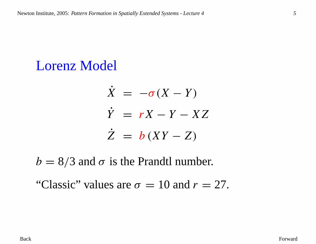
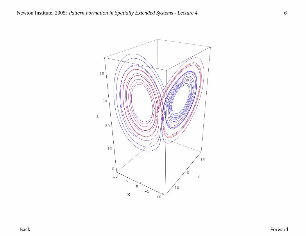
Lorenz Model

X = −σ(X − Y )Y = rX − Y −XZZ = b (XY − Z)

b = 8/3 andσ is the Prandtl number.

“Classic” values areσ = 10 andr = 27.

Back Forward


-10-5

05

10

X

-10

0

10

Y

0

10

20

30

40

Z

-50

510

X

Back Forward


The Butterfly Effect

The “sensitive dependence on initial conditions” found by Lorenz is often

called the “butterfly effect”.

In fact Lorenz first said (Transactions of the New York Academy of

Sciences, 1963)

One meteorologist remarked that if the theory were correct, one flap of the

sea gull’s wings would be enough to alter the course of the weather

forever.

By the time of Lorenz’s talk at the December 1972 meeting of the

American Association for the Advancement of Science in Washington,

D.C. the sea gull had evolved into the more poetic butterfly - the title of

his talk was

Predictability: Does the Flap of a Butterfly’s Wings in Brazil set off a

Tornado in Texas?

Back Forward


Lyapunov Exponents and Eigenvectors

Quantifying the sensitive dependence on initial conditions

t0

t1 t2

t3

tf

δu0

δufX

Y

Z

exponent:λ = lim tf→∞ 1tf−t0 ln

∣∣∣ δufδu0

∣∣∣ ; δuf → eigenvector

Back Forward


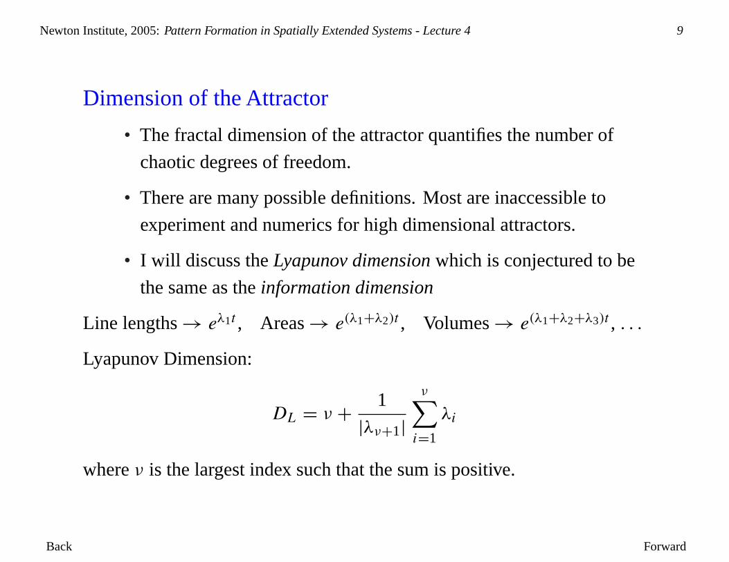
Dimension of the Attractor

• The fractal dimension of the attractor quantifies the number of

chaotic degrees of freedom.

• There are many possible definitions. Most are inaccessible to

experiment and numerics for high dimensional attractors.

• I will discuss theLyapunov dimensionwhich is conjectured to be

the same as theinformation dimension

Line lengths→ eλ1t , Areas→ e(λ1+λ2)t , Volumes→ e(λ1+λ2+λ3)t , . . .

Lyapunov Dimension:

DL = ν + 1

|λν+1|ν∑i=1

λi

whereν is the largest index such that the sum is positive.

Back Forward


Lyapunov dimension

Defineµ(n) =∑ni=1 λi (λ1 ≥ λ2 · · · ) with λi theith Lyapunov

exponent.

DL is the interpolated value ofn givingµ = 0 (the dimension of the

volume that neither grows nor shrinks under the evolution)

Back Forward


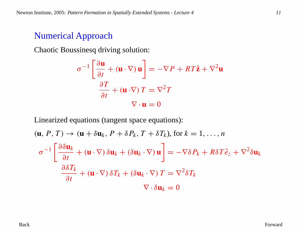
Numerical Approach

Chaotic Boussinesq driving solution:

σ−1[∂u∂t+ (u · ∇)u

]= −∇P + RT z+∇2u

∂T

∂t+ (u ·∇) T = ∇2T

∇ ·u = 0

Linearized equations (tangent space equations):

(u, P , T )→ (u+ δuk, P + δPk, T + δTk), for k = 1, . . . , n

σ−1[∂δuk∂t+ (u · ∇) δuk + (δuk · ∇)u

]= −∇δPk + RδT ez +∇2δuk

∂δTk

∂t+ (u · ∇) δTk + (δuk · ∇) T = ∇2δTk

∇ · δuk = 0

Back Forward


Small system chaos: some experimental highlights

The Lorenz model does not describe Rayleigh-Bénard convection.

However the ideas of low dimensional modelsdoapply to convection,

fluids and other continuum systems.

Ahlers (1974) Transition from time independent flow to aperiodic flow at

R/Rc ∼ 2 (aspect ratio 5)

Gollub and Swinney (1975)Onset of aperiodic flow from time-periodic

flow in Taylor-Couette

Maurer and Libchaber, Ahlers and Behringer (1978) Transition from

quasiperiodic flow to aperiodic flow in small aspect ratio convection

Lichaber, Laroche, and Fauve (1982)Quantitative demonstration of the

Fiegenbaum period doubling route to chaos

Back Forward


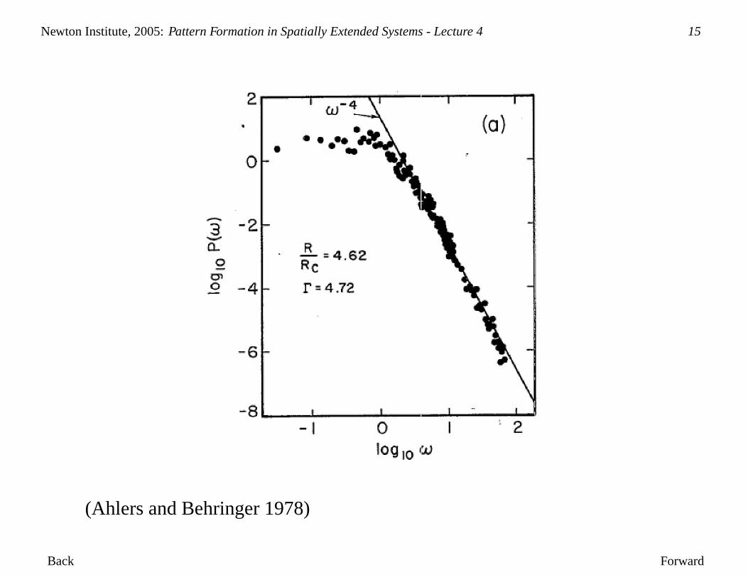
Revisit Ahlers (1974), Ahlers and Behringer (1978)

• First experiments:0 = 5.27 cell, cryogenic (normal) liquidHe4 as

fluid. High precision heat flow measurements (no flow visualization).

• Onset of aperiodic time dependence in low Reynolds number flow:

relevance of chaos to “real” (continuum) systems.

• Power law decrease of power spectrumP(f ) ∼ f−4

• Aspect ratio dependence of the onset of time dependence (Ahlers and

Behringer, 1978)

0 2 5 57

Rt 10Rc 2Rc 1.1Rc

Back Forward


(Ahlers 1974)

Back Forward


(Ahlers and Behringer 1978)

Back Forward


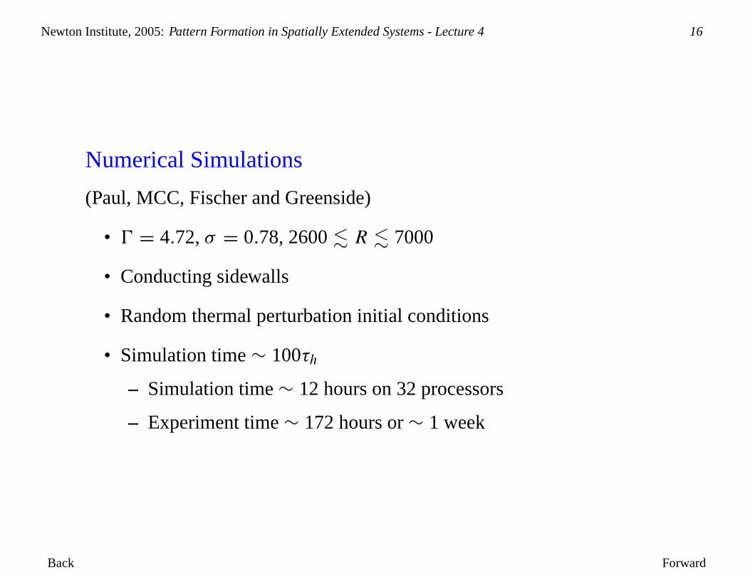
Numerical Simulations

(Paul, MCC, Fischer and Greenside)

• 0 = 4.72,σ = 0.78, 2600. R . 7000

• Conducting sidewalls

• Random thermal perturbation initial conditions

• Simulation time∼ 100τh

– Simulation time∼ 12 hours on 32 processors

– Experiment time∼ 172 hours or∼ 1 week

Back Forward


0 500 1000 1500 2000time

1.4

1.5

1.6

1.7

1.8

1.9

2

Nu

R = 6949R = 4343R = 3474R = 3127R = 2804R = 2606

50 τh

Γ = 4.72σ = 0.78 (Helium)Random Initial Conditions

Back Forward


R = 3127 R = 6949

Back Forward


Power Spectrum

• Simulations oflow dimensional chaos(e.g. Lorenz model) show

exponential decaying power spectrum

• Power law power spectrum easily obtained fromstochasticmodels

(white-noise driven oscillator, etc.)

Deterministic Chaos ?⇒? Exponential decay

Stochastic Noise ?⇒? Power law decay

Back Forward


Simulation yields a power law over the range accessible to experiment

10-2 10-1 100 101 102

ω10-12

10-11

10-10

10-9

10-8

10-7

10-6

P(ω

)

R = 6949ω-4

Γ = 4.72, σ = 0.78, R = 6949Conducting sidewalls

R/Rc = 4.0

Back Forward


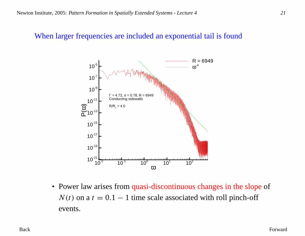
When larger frequencies are included an exponential tail is found

10-2 10-1 100 101 102

ω10-21

10-19

10-17

10-15

10-13

10-11

10-9

10-7

10-5

P(ω

)

R = 6949ω-4

Γ = 4.72, σ = 0.78, R = 6949Conducting sidewalls

R/Rc = 4.0

• Power law arises fromquasi-discontinuous changes in the slopeofN(t) on at = 0.1− 1 time scale associated with roll pinch-offevents.

Back Forward


Lyapunov Exponent

10 20 30 40 500

10

20

30

t

log

|Nor

m|

dataλ = 0.6

Back Forward


Lyapunov eigenvector

Back Forward


Spatiotemporal chaos

Rough definition: the dynamics, disordered in time and space, of a large

aspect ratio system (i.e. one that is large compared to the size of a basic

chaotic element)

• Natural examples

� The atmosphere and ocean (weather, climate etc.)

� Heart fibrillation

• Examples from convection

� Spiral Defect Chaos ( experiment , simulations )

� Domain Chaos (model simulations: stripes , orientations ,

walls ; convection simulations )

Back Forward


Spatiotemporal chaos

Rough definition: the dynamics, disordered in time and space, of a large

aspect ratio system (i.e. one that is large compared to the size of a basic

chaotic element)

• Natural examples

� The atmosphere and ocean (weather, climate etc.)

� Heart fibrillation

• Examples from convection

� Spiral Defect Chaos ( experiment , simulations )

� Domain Chaos (model simulations: stripes , orientations ,

walls ; convection simulations )

Spatiotemporal chaos is a new paradigm of unpredictable dynamics.

(What effect does the butterfly really have?)

Back Forward


Challenges

• System-specific questions

• Definition and characterization

• Transitions to spatiotemporal chaos and between different chaotic

states

• Coarse grained descriptions

• Control

Back Forward


Challenges




states


• Control

Ideas and methods from dynamical systems, statistical mechanics, phase

transition theory …

Back Forward


Systems

• Coupled Maps

x(n+1)i = f (x(n)i )+D × 1

n

∑δ=n.n.

[f (x(n)i+δ)− f (x(n)i )]

with e.g.f (x) = ax(1− x)• PDE simulations

� Kuramoto-Sivashinsky equation

∂tu = −∂2xu− ∂4

xu− u∂xu

� Amplitude equations, e.g. Complex Ginzburg-LandauEquation

∂tA = εA+ (1+ ic1)∇2A− (1− ic3) |A|2A

• Physical systems (experiment and numerics)

Back Forward


Definition and characterization

• Narrow the phenomena

• Decide if theory, simulation, and experiment match

Back Forward


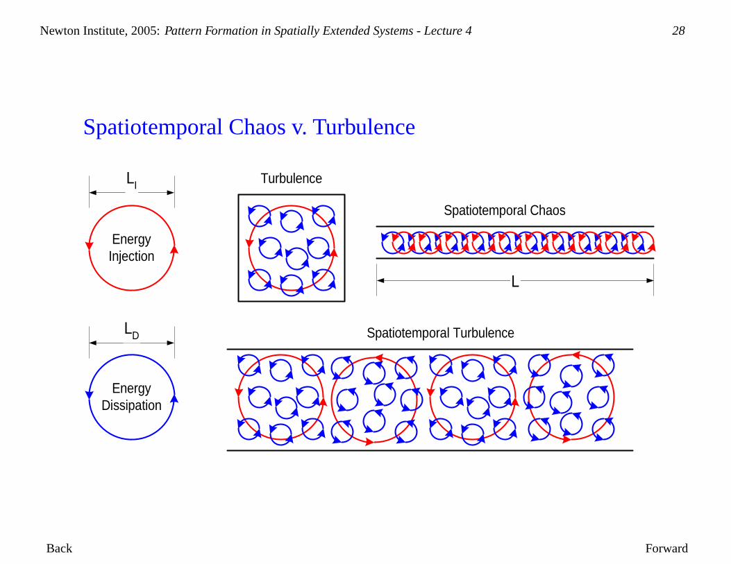
Spatiotemporal Chaos v. Turbulence

EnergyInjection

EnergyDissipation

LI

LD

Turbulence

Spatiotemporal Chaos

Spatiotemporal Turbulence

L

Back Forward


Characterizing spatiotemporal chaos

Methods from statistical physics: Correlation lengths and times, etc.

• Easy to measure, but perhaps not very insightful

Methods from dynamical systems:Lyapunov exponents and attractor

dimensions.

• Inaccessible in experiment, but can be measured in simulations

• Ruelle suggested that Lyapunov exponents should beintensive,

and the dimension should beextensive∝ Ld

Back Forward


Lyapunov spectrum and dimension for spiral defect chaos

(Egolf et al. 2000)

Back Forward


Microextensivity for the 1d Kuramoto-Sivashinsky equation

78 83 88 93L

15

16

17

18

Lyap

unov

Dim

ensi

on

(from Tajima and Greenside 2000)

Back Forward


Microextensivity

Interesting questions:

• Are there (tiny) windows of periodic orbits or chaotic orbits of

non-scaling dimension so that smooth variation is only in theL→∞limit, or is the variation smooth at finiteL?

• Can we use this to define spatiotemporal chaos for finiteL?

• Does spatiotemporal chaos in Rayleigh-Bénard Convection show

microextensive scaling of the Lyapunov dimension?

Back Forward


Lyapunov vector for spiral defect chaos

(from Keng-Hwee Chiam, Caltech thesis 2003)

Back Forward


Challenges




states


• Control

Back Forward


Transitions

In thermodynamic equilibrium systems the behavior may be simpler near

phase transitions.

Is there universal behavior near transitions in spatiotemporal chaos

(transition to STC, transitions within STC)?

If so, is the universality the same as in corresponding equilibrium systems?

Examples:

• Chaotic Ising map

• Rotating convection

Back Forward


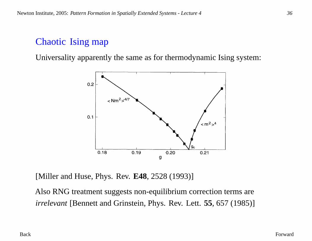
Chaotic Ising map

Universality apparently the same as for thermodynamic Ising system:

[Miller and Huse, Phys. Rev.E48, 2528 (1993)]

Also RNG treatment suggests non-equilibrium correction terms are

irrelevant [Bennett and Grinstein, Phys. Rev. Lett.55, 657 (1985)]

Back Forward


Scaling near onset of domain chaos

Rotat ion Rate

Ray

leig

h N

umbe

r

no pattern(conduction)

stripes(convect ion)

KL

spiralchaos

lockeddomainchaos

(?)

domainchaos

R C

Back Forward


Amplitude equation description(Tu and MCC, 1992)]

Amplitudes of rolls at 3 orientationsAi(r , t), i = 1 . . .3

∂tA1 = εA1+ ∂2x1A1− A1(A

21+ g+A2

2+ g−A23)

∂tA2 = εA2+ ∂2x2A2− A2(A

22+ g+A2

3+ g−A21)

∂tA3 = εA3+ ∂2x3A3− A3(A

23+ g+A2

1+ g−A22)

whereε = (R − Rc(�)/Rc(�)Rescale space, time, and amplitudes:

Back Forward


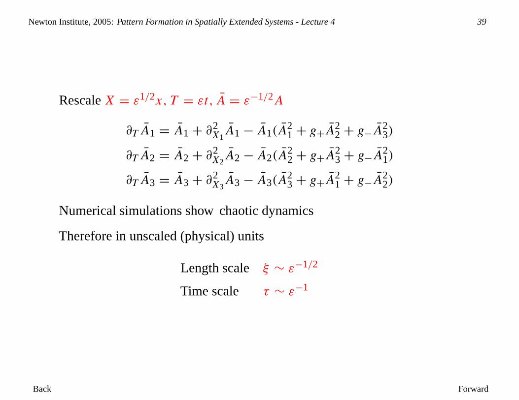
RescaleX = ε1/2x, T = εt, A = ε−1/2A

∂T A1 = A1+ ∂2X1A1− A1(A

21+ g+A2

2+ g−A23)

∂T A2 = A2+ ∂2X2A2− A2(A

22+ g+A2

3+ g−A21)

∂T A3 = A3+ ∂2X3A3− A3(A

23+ g+A2

1+ g−A22)

Numerical simulations show chaotic dynamics

Therefore in unscaled (physical) units

Length scale ξ ∼ ε−1/2

Time scale τ ∼ ε−1

Back Forward


Summary of Tests

• Simulations [MCC and Meiron (1994)] of generalized Swift-Hohenberg

equations in periodic geometries show results consistent with predictions

• [Hu et al. (1995) + others] Experiments give results that are consistent either

with finite values ofξ, τ at onset, of much smaller power laws

ξ ∼ ε−0.2, τ ∼ ε−0.6

• [MCC, Louie, and Meiron (2001)] Simulations of generalized Swift-Hohenberg

equations in circular geometries of radius0 gave results consistent with finite

size scaling

ξM = ξf (0/ξ) with ξ ∼ ε−1/2

• [Scheel and MCC, preprint (2005)] Simulations of Rayleigh-Bénard convection

with Coriolis forces giveτ ∼ ε−1 for small enoughε. For largerε a slower

growth is seen consistent withτ ∼ ε−0.7.

Back Forward


Possible explanations for discrepancies?

• Finite size effects?

• Dislocation glide important (not in Tu-Cross model)?

• Centrifugal force important in experimental geometry?

• … or critical-like fluctuation effects important?

Back Forward


Challenges




states


• Control

Back Forward


Coarse grained description

• Can we find simplified descriptions of spatiotemporal chaotic

systems atlarge length scales?

� conserved quantity (cf. hydrodynamics)

� near continuous transition

� collective motion such as defects

• Is the simplified description analogous to a thermodynamic

equilibrium system?

Back Forward


Rough argument

Back Forward


Rough argument

Expect a Langevin description at large scales

∂ty = D(y)+ η

y is vector of large length scale variables,D is some effective deterministic dynamics,

andη is noise coming from small scale chaotic dynamics.

Back Forward


Rough argument


∂ty = D(y)+ η



Sinceη represents the effect of many small scale fast chaotic degrees of freedom acting

on the large scales we might expect it to be Gaussian and white⟨ηi(r , t)ηj (r ′, t ′)

⟩ = �ij δ(r − r ′)δ(t − t ′)

Back Forward


Rough argument


∂ty = D(y)+ η





⟩ = �ij δ(r − r ′)δ(t − t ′)

In systems deriving from a microscopicHamiltoniandynamicsconstraintsrelate the

noise�ij and the deterministic termsD (the fluctuation-dissipation theorem).

Back Forward


Rough argument


∂ty = D(y)+ η





⟩ = �ij δ(r − r ′)δ(t − t ′)

In systems deriving from a microscopicHamiltoniandynamicsconstraintsrelate the

noise�ij and the deterministic termsD (the fluctuation-dissipation theorem).

In systems based on adissipativesmall scale dynamics,if the dominant macroscopic

dynamics is sufficiently simple, or sufficiently constrained by symmetries, these

relationships mayhappento occur.

Back Forward


Examples

• Chaotic Kuramoto-Sivashinsky dynamics reduces to noisy

Burgers equation [Zaleski (1989)]

• Chaotic Ising map model near the transition

� Langevin equation for dynamics of domain walls same as in

equilibrium system [Miller and Huse, (1993)]

� Coarse grained configurations satisfy detailed balance and

have a distribution given by an effective free energy [Egolf,

Science287, 101 (2000)]

• Defect dynamics description of 2D Complex Ginzburg Landau

chaos [Brito et al., Phys. Rev. Lett.90, 063801 (2003)]

Back Forward


Conclusions

In this lecture I introduced some of the basic ideas of chaos, and discussed

the application of these ideas to continuum systems.

I reviewed some old experiments on chaos in continuum systems, together

with recent numerical results on these systems.

I then introduced spatiotemporal chaos, which remains a poorly

characterized and understood phenomenon. The careful comparison

between experiment, theory, and numerics has been and will continue to

be important in increasing our understanding.

Documents

Pattern Formation in Spatially Extended Systems Lecture 4mcc/MiniCourse/NI_lecture4_slides.pdf · Back Forward Newton Institute, 2005: Pattern Formation in Spatially Extended Systems