PATTERN FORMATION FINITE ELEMENT MODELING …congress.cimne.com/iacm-eccomas2014/admin/files/filePaper/p909.pdf · FAN XU∗,†, SALIM BELOUETTAR∗ AND MICHEL POTIER-FERRY ... the

11th World Congress on Computational Mechanics (WCCM XI)5th European Conference on Computational Mechanics (ECCM V)

6th European Conference on Computational Fluid Dynamics (ECFD VI)E. Onate, J. Oliver and A. Huerta (Eds)

PATTERN FORMATION FINITE ELEMENT MODELINGFOR THIN FILMS ON SOFT SUBSTRATES

FAN XU∗,†, SALIM BELOUETTAR∗ AND MICHEL POTIER-FERRY†

∗ Centre de Recherche Public Henri Tudor29 Avenue John F. Kennedy, L-1855 Luxembourg-Kirchberg, Luxembourg

e-mail: [email protected], [email protected]

† Laboratoire d’Etude des Microstructures et de Mecanique des MateriauxLEM3, UMR CNRS 7239, Universite de Lorraine

Ile du Saulcy, 57045 Metz Cedex 01, Francee-mail: [email protected], [email protected]

Key words: Wrinkling, Post-buckling, Bifurcation, Path-following Perturbation Tech-nique, Herringbone Pattern, Finite Element Method.

Abstract. Spatial pattern formation of stiff thin films on compliant substrates is inves-tigated based on a nonlinear 3D finite element model. The resulting nonlinear equationsare then solved by the Asymptotic Numerical Method (ANM) that gives interactive accessto semi-analytical equilibrium branches, which offers considerable advantages in terms ofcomputation time and reliability compared with classical iterative algorithms. Bifurcationpoints on nonlinear response curves are detected through computing bifurcation indica-tors well adapted to the ANM. The occurrence and post-buckling evolution of sinusoidaland herringbone patterns will be highlighted.

1 INTRODUCTION

Wrinkles of stiff thin layers attached on soft substrates have been widely observed innature and these phenomena have raised considerable interests over the last decade. Thepioneering work of Bowden et al. [1] leads to several theoretical and numerical works interms of stability study devoted to linear perturbation analysis and nonlinear bucklinganalysis [2, 3, 4]. Nevertheless, most previous studies have been mainly constrained todetermine the critical conditions of instability and corresponding wrinkling patterns nearthe instability threshold in 2D cases. The post-buckling evolution and mode transitionof surface wrinkles in 3D cases are only recently being pursued [5]. However, the 3Dfilm/substrate systems with real boundary conditions but not periodic cells are rarelystudied, especially through numerical ways that can provide the overall view and insightinto the formation and evolution of wrinkle patterns.

1

Fan Xu, Salim Belouettar and Michel Potier-Ferry

This study aims at applying advanced numerical methods for bifurcation analysis totypical film/substrate models and focuses on the post-bifurcation evolution involving sec-ondary bifurcations and advanced modes, for the first time with a particular attentionon the effect of boundary conditions. For this purpose, a 2D finite element (FE) mod-el was previously developed for multiperiodic bifurcation analysis of wrinkle formation[6]. In this model, the film undergoing moderate deflections is described by Foppl-vonKarman nonlinear elastic theory, while the substrate is considered to be a linear elasticsolid. Following the same strategy, we extend the work to 3D cases by coupling shellelements representing the film and block elements describing the substrate. Therefore,large rotations and deformations in the film can be considered and the spatial distributionof wrinkling modes like stripe, checkerboard or herringbone could be investigated.

The morphological post-buckling evolution and mode shape transition beyond the criti-cal load are incredibly complicated, especially in 3D cases, and the conventional numericalmethods have difficulties in detecting all the bifurcation points and associated instabilitymodes on their evolution paths. To solve the resulting nonlinear equations, we adoptedthe Asymptotic Numerical Method (ANM) [7, 8] which appears as a significantly efficientcontinuation technique without any corrector iteration. The underlying principle of theANM is to build up the nonlinear solution branch in the form of relatively high ordertruncated power series. Since few global stiffness matrix inversions are required (only oneper step), the performance in terms of computing time is quite attractive. Moreover, un-like incremental-iterative methods, the arc-length step size in the ANM is fully adaptivesince it is determined a posteriori by the algorithm. A small radius of convergence andstep accumulation appear around the bifurcation and imply its presence. Furthermore, abifurcation indicator [9, 10] well adapted to the ANM, is computed to detect the exactbifurcation points. This indicator measures the intensity of the system response to per-turbation forces. By evaluating it through an equilibrium branch, all the critical pointsexisting on this branch and the associated bifurcation modes can be determined.

2 3D MODEL

We consider an elastic thin film bonded to an elastic substrate, which can buckle undercompressions. Upon wrinkling, the film elastically buckles to relax the compressive stressand the substrate concurrently deforms to maintain perfect bonding at the interface. Inthe following, the elastic potential energy of the system, is considered in the frameworkof Hookean elasticity. The film/substrate system is considered to be three-dimensionaland the geometry is as shown in Fig. 1a. Let x and y be in-plane coordinates, while zis the direction perpendicular to the mean plane of the film/substrate. The width andlength of the system are denoted by Lx and Ly, respectively. The parameters hf , hs andht represent, respectively, the thickness of the film, the substrate and the total thicknessof the system. Young’s modulus and Poisson’s ratio of the film are denoted by Ef andνf , while Es and νs are the corresponding material properties for the substrate.

2


(a) (b)

Figure 1: (a) Geometry of film/substrate system. (b) Geometry and kinematics of shell.

2.1 Nonlinear shell formulation for the film

Challenges in the numerical modeling of such film/substrate systems come from theextremely large ratio of Young’s modulus (Ef/Es ≈ O(105)) as well as the big thicknessdifference (hs/hf > O(102)), which requires very fine mesh if using 3D block elementsboth for the film and for the substrate. Since finite rotations of middle surface and smallstrains are considered in the thin film, the nonlinear shell formulation is quite suitable andefficient for modeling. Hereby, a three-dimensional shell formulation proposed by Buchteret al. [11] is applied. It is based on a 7-parameter theory including a linear varyingthickness stretch as extra variable, which permits to apply a complete 3D constitutive lawwithout condensation. It is also incorporated via the Enhanced Assumed Strain (EAS)concept proposed by Simo and Rifai [12] to improve the element performance and to avoidlocking phenomena such as Poisson thickness locking, shear locking or volume locking.Since there is no required inter element continuity, the extra variable is eliminated at theelement level and then it preserves the formal structure of a 6-parameter shell theory. Thishybrid shell formulation can describe large deformation problems with hyperelasticity andhas been successively applied to nonlinear elastic thin-walled structures such as cantileverbeam, square plate, cylindrical roof and circular deep arch [13, 10].

Geometry and kinematics of this shell element are illustrated in Fig. 1b, where the posi-tion vectors are described by curvilinear coordinates (θ1, θ2, θ3). The geometry descriptionrelies on the middle surface θ1 and θ2 of the shell, while θ3 represents the coordinate in thethickness direction. The current configuration is defined by the middle surface displace-ment and the relative displacement between the middle and the upper surfaces. The largerotations are taken into account without any rotation matrix since the current directionvector is obtained by adding a simple vector to one of the initial configurations.

In the initial undeformed configuration, the position vector x representing any pointin the shell can be defined as

x(θα, θ3) = r(θα) + θ3a3(θα), (1)

where r(θα)(α = 1, 2) denotes the projection of x in the middle surface and θ3 describesits perpendicular direction with θ3 ∈ [−hf/2, hf/2] in which hf is the reference thickness

3


of shell. The normal vector of middle surface is represented by a3 = a1×a2. The covariantbase vectors defined by middle surface are derived as

gα = x,α = aα + θ3a3,α with aα = r,α,g3 = x,3 = a3.

(2)

Similarly, in the current deformed configuration, we define the position of point x bythe vector x:

x(θα, θ3) = r(θα) + θ3a3(θα), (3)

where r = r+ v,a3 = a3 +w.

(4)

Therefore, the displacement vector that linearly varies along the thickness direction reads

u(θα, θ3) = x− x = v(θα) + θ3w(θα). (5)

Analogous to the definition in (2), the covariant base vectors in the current deformedconfiguration can be defined as

gα = x,α = aα + θ3a3,α with aα = r,α,g3 = x,3 = a3.

(6)

The nonlinear Green−Lagrange strain tensor in the covariant base reads

γ =1

2

(gij − gij

)gi ⊗ gj with i, j = 1, 2, 3, (7)

where gi are the contravariant base vectors, while gij = gi ·gj and gij = gi ·gj respectivelyrepresent the components of covariant metric tensor in the initial configuration and thedeformed one [11].

The hybrid shell formulation is derived from a three-field variational principle basedon the Hu−Washizu functional [13]. The stationary condition can be written as

ΠEAS (u, γ,S) =

∫

Ω

tS : (γu + γ)−

1

2tS : D−1 : S

dΩ− λPe(u), (8)

where D is the elastic stiffness tensor. The unknowns are, respectively, the displacementfield u, the second Piola−Kirchhoff stress tensor S and the compatible Green−Lagrangestrain γu that can be decomposed into a linear part and a quadratic one (γu = γl(u) +γnl(u,u)). The enhanced assumed strain, γ, is orthogonal to the stress field. The workof external load is denoted by Pe(u), while λ is a scalar load parameter.

The variational problem of (8) reads

δΠEAS (u, γ,S) =

∫

Ω

tδS :

[(γu + γ)−D−1 : S

]+ tS : [δγu + δγ]

dΩ− λPe(δu) = 0.

(9)

4


The above equation can be rewritten in a general nonlinear problem form:

R (U, λ) = L (U) +Q (U,U)− λF = 0, (10)

where U = (u, γ,S) is a mixed vector of unknowns, L(·) a linear operator, Q(·, ·) aquadratic one, F the external load vector and R the residual vector. The introducedoperators are linked to the following variables:

〈L (U) , δU〉 =

∫

Ω

tδS :

[γl(u) + γ −D−1 : S

]+ tS : [γl (δu) + δγ]

dΩ,

〈Q (U,U) , δU〉 =

∫

Ω

tδS : γnl (u,u) +

tS : 2γnl (u, δu)dΩ,

〈F, δU〉 = Pe(δu).

(11)

The above quadratic forms are well suitable for asymptotic expansions that will be intro-duced in Section 3.

2.2 Linear elasticity for the substrate

Since the displacement, rotation and strain remain relatively small in the substrate,the linear isotropic elasticity theory with updated geometry can accurately describe thesubstrate. The nonlinear strain-displacement behavior has essentially no influence on theresults of interest [2].

2.3 Connection between the film and the substrate

As the film is bonded to the substrate, the displacement should be continuous at theinterface. However, the shell elements for the film and 3D block elements for the substratecan not be simply joined directly since they belong to dissimilar elements. Therefore,additional incorporating constraint equations have to be employed. Hereby, Lagrangemultipliers, ℓ, are applied to couple the corresponding node displacements in compatiblemeshes between the film and the substrate. The stationary function of film/substratesystem is given in a Lagrangian form as

L (uf ,us, ℓ) = ΠEAS +Πs +∑

node i

ℓi

[u

−f (i)− us(i)

], (12)

where

u−f (i) = v(i)−

hf

2w(i). (13)

From (12), three equations are obtained according to δuf , δus and δℓ:

δΠEAS +∑

node i

ℓiδu−f (i) = 0,

δΠs −∑

node i

ℓiδus(i) = 0,

∑

node i

δℓiu−f (i)−

∑

node i

δℓius(i) = 0.

(14)

5


3 RESOLUTION TECHNIQUE AND BIFURCATION ANALYSIS

The ANM [7, 8] is used to solve the resulting nonlinear equations, which is a path-following technique based on the succession of high order power series expansions (pertur-bation technique) with respect to a well chosen path parameter. It appears as an efficientcontinuation predictor without any corrector iteration. One can get approximations of thesolution path that are very accurate inside the radius of convergence. In this paper, themain interest of the ANM is its ability to detect bifurcation points. First, small steps areoften associated with the occurrence of a bifurcation. Then, a bifurcation indicator willbe defined, which permits to exactly detect the bifurcation load and the correspondingnonlinear mode.

3.1 Path-following technique

Let us recall the generalized nonlinear problem defined in (10). The principle of theANM continuation consists in describing the solution path by computing a succession oftruncated power series expansions. From a known solution point (U0, λ0), the solution(U, λ) is expanded into truncated power series of a perturbation parameter a:

U(a) = U0 + aU1 + a2U2 + . . .+ anUn, (15)

λ(a) = λ0 + aλ1 + a2λ2 + . . .+ anλn, (16)

a = 〈u− u0,u1〉+ (λ− λ0)λ1, (17)

where n is the truncation order of the series. The equation (17) defines the path parametera that can be identified to an arc-length parameter. By introducing (15) and (16) into(10) and (17), then equating the terms at the same power of a, one can obtain a set oflinear problems:

Order 1 :L0

t (U1) = λ1F, (18)

〈u1,u1〉+ λ21 = 1. (19)

Order p > 2 :

L0t (Up) = λpF−

p−1∑

r=1

Q (Ur,Up−r) , (20)

〈up,u1〉+ λpλ1 = 0, (21)

where L0t (·) = L(·) + 2Q(U0, ·) is the linear tangent operator. Note that this operator

depends only on the initial solution and takes the same value for every order p, whichleads to only one matrix inversion at each step. These linear problems are solved by FEmethod. Once the value of Up is calculated, the path solution at the step (j + 1) can beobtained through (15).

6


The maximum value of the path parameter a is automatically defined by analyzing theconvergence of the power series at each step. The amax can be based on the differenceof displacements at two successive orders that must be smaller than a given precisionparameter ǫ:

V alidity range : amax =

(ǫ‖u1‖

‖un‖

) 1

n−1

, (22)

where the notation ‖·‖ stands for the Euclidean norm. Unlike incremental-iterative meth-ods, the arc-length step size amax is adaptive since it is determined a posteriori by thealgorithm. When there is a bifurcation point on the solution path, the radius of conver-gence is defined by the distance to the bifurcation. Thus, the step length defined in (22)becomes smaller and smaller, which looks as if the continuation process ‘knocks’ againstthe bifurcation [14]. This accumulation of small steps is a very good indicator of thepresence of a singularity on the path. All the bifurcations can be easily identified in thisway by the user without any special tool.

3.2 Detection of bifurcation points

The detection of exact bifurcation points is really a challenge. It takes much computa-tion time in the bisection sequence and in many Newton−Raphson iterations due to smallsteps close to the bifurcation. In the framework of the ANM, a bifurcation indicator hasbeen proposed to capture exact bifurcation points in an efficient and reliable algorithm[9, 10].

Let ∆µf be a fictitious perturbation force applied to the structure at a given deformedstate (U, λ), where ∆µ is the intensity of the force f and ∆U is the associated response.Through superposing the applied load and perturbation, the fictitious perturbed equilib-rium can be described by

L (U+∆U) +Q (U +∆U,U+∆U) = λF+∆µf . (23)

Considering the equilibrium state and neglecting the quadratic terms, one can obtain thefollowing auxiliary problem:

Lt (∆U) = ∆µf , (24)

where Lt(·) = L(·) + 2Q(U, ·) is the tangent operator at the equilibrium point (U, λ). If∆µ is imposed, this leads to a displacement tending to infinity in the vicinity of the criticalpoints. To avoid this problem, the following displacement based condition is imposed:

⟨L0

t (∆U−∆U0) ,∆U0

⟩= 0, (25)

where L0t (·) is the tangent operator at the starting point (U0, λ0) and the direction ∆U0

is the solution of L0t (∆U0) = f . Consequently, ∆µ is deduced from the linear system (24)

and (25):

∆µ =〈∆U0, f〉

〈L−1t (f), f〉

. (26)

7


Since the scalar function ∆µ represents a measure of the stiffness of structure and be-comes zero at the singular points, it can define a bifurcation indicator. It can be directlycomputed from (26) but it requires to decompose the tangent operator at each pointthroughout the solution path. For this reason, the system (24) and (25) can be moreefficiently resolved by the ANM, which is detailed in [6].

4 NUMERICAL RESULTS

Two types of wrinkling patterns, sinusoidal and herringbone mode, will be investigatedunder different loading and boundary conditions. On the bottom surface of the substrate,the deflection uz and the tangential traction are taken to be zero. The material andgeometric parameters of film/substrate system are similar to those in [1, 6], which is shownin Table 1. The huge ratio of Young’s modulus, Ef/Es, determines the critical wavelengthλc that remains practically unchanged as the amplitude of the wrinkles increases [3, 6].Poisson’s ratio is a dimensionless measure of the degree of compressibility. Compliantmaterials in the substrate, such as elastomers, are nearly incompressible with νs = 0.48.A relative thin film has been chosen so that an isotropic and homogeneous system is notparameter dependent [6]. In order to trigger a transition from the fundamental branch tothe bifurcated one, small perturbation forces, fz = 10−8, are imposed in the film. Criticalloads can be detected by bifurcation points in the load-displacement curve. The numberof elements required for a convergent solution was carefully examined.

Table 1: Material and geometric parameters of film/substrate systems

Ef Es νf νs Lx Ly hf hs

(MPa) (MPa) (mm) (mm) (mm) (mm)Film/Sub I 1.3× 105 1.8 0.3 0.48 1.5 1.5 10−3 0.1Film/Sub II 1.3× 105 1.8 0.3 0.48 0.75 1.5 10−3 0.1

4.1 Sinusoidal patterns

First, we study the sinusoidal pattern formation and evolution via Film/Sub I. Thefilm/substrate is under uniaxial compression along the x direction, where the displace-ments, uy and uz on loading sides Ly, are taken to be zero (uy = uz = 0).

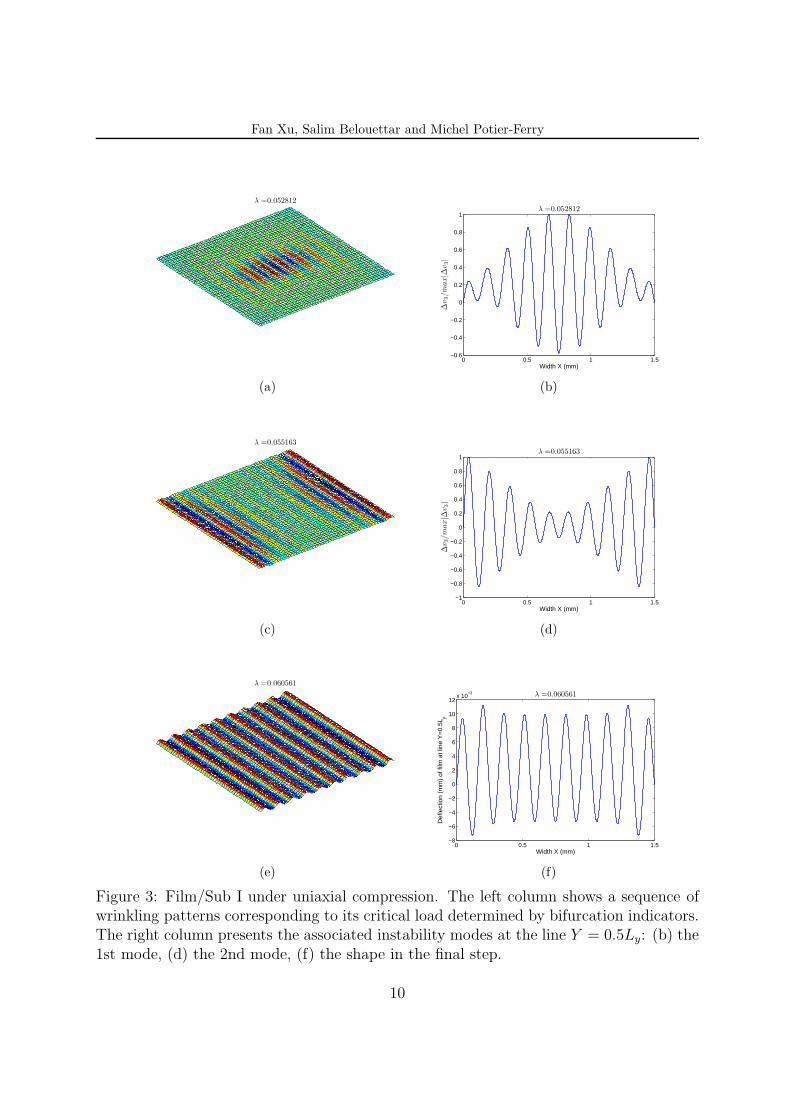
Although the small step accumulation is a good indicator of the occurrence of bifurca-tion, the exact bifurcation points may locate between the neighbouring two steps, whichcan not be captured directly. Therefore, bifurcation indicators are computed to detect theexact position of bifurcation points. By evaluating this indicator through an equilibriumbranch, all the critical points existing on this branch (see Fig. 2a) and the associatedbifurcation modes (see Fig. 3) can be determined. The first two modes correspond tomodulated oscillations, the first one with a sinusoidal envelope and the second one with ahyperbolic tangent shape due to boundary effects. When the loads increase, the pattern

8


tends to be a uniform sinusoidal shape in the bulk in the final step.

0 0.01 0.02 0.03 0.04 0.05 0.06−6

−5

−4

−3

−2

−1

0

1x 10

−3

Def

lect

ion

(mm

) in

the

film

cen

ter

Load (N/mm)

0.052 0.053 0.054 0.055 0.056

−3

−2

−1

0

1x 10

−4

2nd bifurcation

1st bifurcation

(a)

0 0.01 0.02 0.03 0.04 0.05 0.06 0.07 0.08 0.09 0.18.2

8.3

8.4

8.5

8.6

8.7

8.8

8.9

9

9.1x 10

−3

Def

lect

ion

(mm

) in

the

film

cen

ter

Load (N/mm)

1st bifurcation

2nd bifurcation

(b)

Figure 2: (a) Bifurcation curve of Film/Sub I under uniaxial compression. (b) Bifurcationcurve of Film/Sub II under the second step compression along the y direction.

4.2 Herringbone patterns

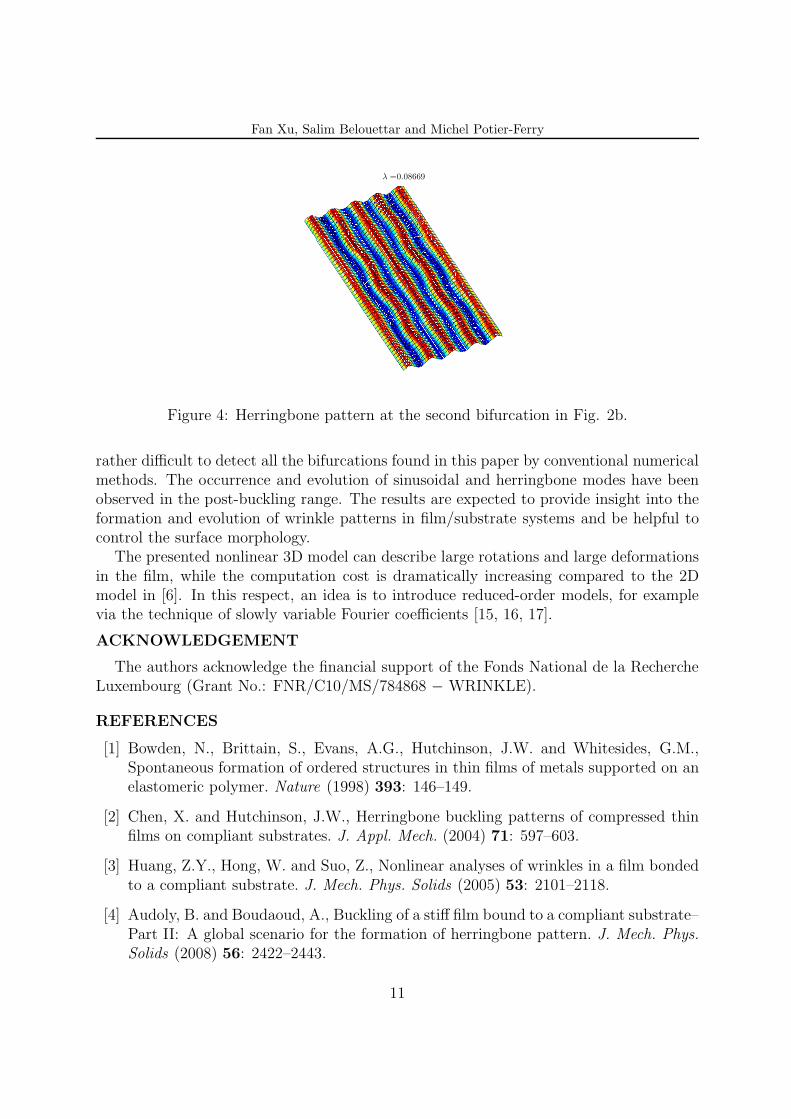
Herringbone modes are investigated via Film/Sub II with a rectangular surface (Lx/Ly =0.5) so as to more clearly observe the patterns, since the wavelength λx and λy are notidentical. The film/substrate system is under biaxial step loading. More precisely, thesystem is uniaxially compressed along the x direction at the first step. Then, ux alongthe two sides Ly, are locked at the beginning of the second step. Compressions are thenimposed along the y direction.

The fist step loading generates the same type of sinusoidal wrinkles as in Section 4.1. Atthe second step loading, two bifurcations (see Fig. 2b) have been captured by computingbifurcation indicators. The herringbone mode (see Fig. 4) appears around the secondbifurcation. More details on pattern evolution and further discussions will be presentedelsewhere in our forthcoming papers.

5 CONCLUSION

Pattern formation and evolution of stiff films bound to compliant substrates were in-vestigated, by accounting for boundary conditions in 3D cases, which was rarely studiedpreviously. A classical model was applied associating linear elasticity in the substrate andgeometrically nonlinear shell formulation for the film. Then the shell elements and blockelements were coupled by Lagrange multipliers. The presented results rely heavily on ro-bust solution techniques based on the ANM that is able to detect secondary bifurcationsand to compute bifurcation modes on a nonlinear response curve. Probably, it would be

9


λ =0.052812

(a)

0 0.5 1 1.5−0.6

−0.4

−0.2

0

0.2

0.4

0.6

0.8

1

Width X (mm)

∆v3/m

ax|∆

v3|

λ =0.052812

(b)

λ =0.055163

(c)

0 0.5 1 1.5−1

−0.8

−0.6

−0.4

−0.2

0

0.2

0.4

0.6

0.8

1

Width X (mm)

∆v3/m

ax|∆

v3|

λ =0.055163

(d)

λ =0.060561

(e)

0 0.5 1 1.5−8

−6

−4

−2

0

2

4

6

8

10

12x 10

−3

Width X (mm)

Def

lect

ion

(mm

) of

film

at l

ine

Y=

0.5L

y

λ =0.060561

(f)

Figure 3: Film/Sub I under uniaxial compression. The left column shows a sequence ofwrinkling patterns corresponding to its critical load determined by bifurcation indicators.The right column presents the associated instability modes at the line Y = 0.5Ly: (b) the1st mode, (d) the 2nd mode, (f) the shape in the final step.

10


λ =0.08669

Figure 4: Herringbone pattern at the second bifurcation in Fig. 2b.

rather difficult to detect all the bifurcations found in this paper by conventional numericalmethods. The occurrence and evolution of sinusoidal and herringbone modes have beenobserved in the post-buckling range. The results are expected to provide insight into theformation and evolution of wrinkle patterns in film/substrate systems and be helpful tocontrol the surface morphology.

The presented nonlinear 3D model can describe large rotations and large deformationsin the film, while the computation cost is dramatically increasing compared to the 2Dmodel in [6]. In this respect, an idea is to introduce reduced-order models, for examplevia the technique of slowly variable Fourier coefficients [15, 16, 17].

ACKNOWLEDGEMENT

The authors acknowledge the financial support of the Fonds National de la RechercheLuxembourg (Grant No.: FNR/C10/MS/784868 − WRINKLE).

REFERENCES

[1] Bowden, N., Brittain, S., Evans, A.G., Hutchinson, J.W. and Whitesides, G.M.,Spontaneous formation of ordered structures in thin films of metals supported on anelastomeric polymer. Nature (1998) 393: 146–149.

[2] Chen, X. and Hutchinson, J.W., Herringbone buckling patterns of compressed thinfilms on compliant substrates. J. Appl. Mech. (2004) 71: 597–603.

[3] Huang, Z.Y., Hong, W. and Suo, Z., Nonlinear analyses of wrinkles in a film bondedto a compliant substrate. J. Mech. Phys. Solids (2005) 53: 2101–2118.

[4] Audoly, B. and Boudaoud, A., Buckling of a stiff film bound to a compliant substrate–Part II: A global scenario for the formation of herringbone pattern. J. Mech. Phys.

Solids (2008) 56: 2422–2443.

11


[5] Cai, S., Breid, D., Crosby, A.J., Suo, Z. and Hutchinson, J.W., Periodic patterns andenergy states of buckled films on compliant substrates. J. Mech. Phys. Solids (2011)59: 1094–1114.

[6] Xu, F., Potier-Ferry, M., Belouettar, S. and Hu, H., Multiple bifurcations in wrinklinganalysis of thin films on compliant substrates. Submitted, 2014.

[7] Cochelin, B., Damil, N. and Potier-Ferry, M., Asymptotic-numerical methods andPade approximants for non-linear elastic structures. Int. J. Numer. Meth. Eng. (1994)37: 1187–1213.

[8] Cochelin, B., Damil, N. and Potier-Ferry, M., Methode asymptotique numerique.Hermes Science Publications, 2007.

[9] Vannucci, P., Cochelin, B., Damil, N. and Potier-Ferry, M., An asymptotic-numericalmethod to compute bifurcating branches. Int. J. Numer. Meth. Eng. (1998) 41: 1365–1389.

[10] Boutyour, E.H., Zahrouni, H., Potier-Ferry, M. and Boudi, M., Bifurcation points andbifurcated branches by an asymptotic numerical method and Pade approximants. Int.J. Numer. Meth. Eng. (2004) 60: 1987–2012.

[11] Buchter, N., Ramm, E. and Roehl, D., Three-dimensional extension of non-linearshell formulation based on the Enchanced Assumed Strain concept. Int. J. Numer.

Meth. Eng. (1994) 37: 2551–2568.

[12] Simo, J.C. and Rifai, M.S., A class of mixed assumed strain methods and method ofincompatible modes. Int. J. Numer. Meth. Eng. (1990) 37: 1595–1636.

[13] Zahrouni, H., Cochelin, B. and Potier-Ferry, M., Computing finite rotations of shellsby an asymptotic-numerical method. Comput. Methods Appl. Mech. Engrg. (1999)175: 71–85.

[14] Baguet, S. and Cochelin, B., On the behaviour of the ANM continuation in thepresence of bifurcations. Commun. Numer. Meth. Eng. (2003) 19: 459–471.

[15] Damil, N. and Potier-Ferry, M., Influence of local wrinkling on membrane behaviour:A new approach by the technique of slowly variable Fourier coefficients. J. Mech.

Phys. Solids (2010) 58: 1139–1153.

[16] Mhada, K., Braikat, B., Hu, H., Damil, N. and Potier-Ferry, M., About macroscopicmodels of instability pattern formation. Int. J. Solids Struct. (2012) 49: 2978–2989.

[17] Damil, N., Potier-Ferry, M. and Hu, H., Membrane wrinkling revisited from a multi-scale point of view. Adv. Model. Simul. Eng. Sci. (2014) 1: 6.

12

Documents

PATTERN FORMATION FINITE ELEMENT MODELING …congress.cimne.com/iacm-eccomas2014/admin/files/filePaper/p909.pdf · FAN XU∗,†, SALIM BELOUETTAR∗ AND MICHEL POTIER-FERRY ... the