Submitted 30 November 2012Accepted 28 May 2013Published 25 June 2013

Corresponding authorAlice C. McHardy,alice.mchardy@uni-duesseldorf.de

Academic editorKeith Crandall

Additional Information andDeclarations can be found onpage 14

DOI 10.7717/peerj.89

Copyright2013 Gregor et al.

Distributed underCreative Commons CC-BY 3.0

OPEN ACCESS

PTree: pattern-based, stochastic searchfor maximum parsimony phylogeniesIvan Gregor1, Lars Steinbruck2 and Alice C. McHardy1,2

1 Max-Planck Research Group for Computational Genomics and Epidemiology, Max-PlanckInstitute for Informatics, Saarbrucken, Germany

2 Department of Algorithmic Bioinformatics, Heinrich-Heine-University Dusseldorf,Dusseldorf, Germany

ABSTRACTPhylogenetic reconstruction is vital to analyzing the evolutionary relationship ofgenes within and across populations of different species. Nowadays, with next gen-eration sequencing technologies producing sets comprising thousands of sequences,robust identification of the tree topology, which is optimal according to standardcriteria such as maximum parsimony, maximum likelihood or posterior probability,with phylogenetic inference methods is a computationally very demanding task.Here, we describe a stochastic search method for a maximum parsimony tree, im-plemented in a software package we named PTree. Our method is based on a newpattern-based technique that enables us to infer intermediate sequences efficientlywhere the incorporation of these sequences in the current tree topology yields a phy-logenetic tree with a lower cost. Evaluation across multiple datasets showed that ourmethod is comparable to the algorithms implemented in PAUP* or TNT, which arewidely used by the bioinformatics community, in terms of topological accuracy andruntime. We show that our method can process large-scale datasets of 1,000–8,000sequences. We believe that our novel pattern-based method enriches the current setof tools and methods for phylogenetic tree inference. The software is available under:http://algbio.cs.uni-duesseldorf.de/webapps/wa-download/.

Subjects Bioinformatics, Computational Biology, Evolutionary StudiesKeywords Phylogeny reconstruction, Maximum parsimony, Local search, Stochastic search

INTRODUCTIONPhylogenetic analysis infers the evolutionary relationships among genes from within

or across distinct populations of different species. As input, we are often given a set

of aligned genetic sequences for which we wish to work out the pattern of ancestry.

This analysis plays an important role in, for example, drug or vaccine development

(McHardy & Adams, 2009; Russell et al., 2008). With the cost of sequencing decreasing

rapidly due to next generation sequencing technologies (Metzker, 2010), more and more

sequences are becoming available and deposited in sequence repositories such as GenBank

(Benson et al., 2011). Therefore, new, fast and accurate methods capable of handling

large-scale datasets are required (Sanderson, 2007).

Commonly used methods for phylogenetic inference fall into four categories:

distance-based methods, maximum parsimony, maximum likelihood and Bayesian

How to cite this article Gregor et al. (2013), PTree: pattern-based, stochastic search for maximum parsimony phylogenies. PeerJ 1:e89;DOI 10.7717/peerj.89

methods. Distance-based methods are data clustering methods that consider only the

pairwise measure of evolutionary distances among sequences. Maximum parsimony

assumes that the correct phylogenetic tree is the one requiring the smallest number of

evolutionary events to explain the input sequences. A maximum likelihood method

requires a substitution model to assess the probability of particular phylogenetic trees,

where it aims to find a tree with the highest likelihood with respect to the given substitution

model. Bayesian methods rely on probabilistic models of sequence evolution, like

maximum likelihood tree inference. Different from maximum likelihood estimates,

however, trees are constructed for instance based on the consensus of a set of trees sampled

from the highest probability regions of the posterior distribution over evolutionary model

parameters and trees. There are several software packages that implement variants of these

methods: PHYLIP (Felsenstein, 2005), PAUP* (Swofford, 2002), TNT (Goloboff, Farris &

Nixon, 2008), PSODA (Carroll et al., 2009), POY (Varon, Vinh & Wheeler, 2010), MEGA5

(Tamura et al., 2011) and MRBAYES (Huelsenbeck & Ronquist, 2001).

Maximum likelihood and Bayesian methods are considered to be the most accurate,

and are nowadays relatively fast due to the computational capacity of modern computers

and methodological advances (Guindon & Gascuel, 2003; Huelsenbeck & Ronquist, 2001;

Stamatakis, Ludwig & Meier, 2005; Zwickl, 2006). However, these methods depend on large

numbers of parameters that have to be estimated, such as branch lengths, tree topology,

parameters of the substitution model and site-specific rate variations, which make them

even more computationally demanding. Although maximum likelihood methods are

widely used, Kuck et al. (2012) showed that the high confidence in maximum likelihood

trees is not always justified for certain tree shapes. Distance-based methods, such as the

unweighted pair group method with arithmetic mean (UPGMA) and the neighbor-joining

(NJ) algorithm, are quite fast, with runtime depending only quadratically and cubically,

respectively, on the number of input sequences (Saitou & Nei, 1987; Sokal & Michener,

1958). However, distance-based methods are less accurate than all other techniques. We

here have focused on the maximum parsimony criterion for tree inference, since this

approach has a reasonable trade-off between speed and accuracy and is still considered as

an important optimality criterion for the evaluation of phylogenetic trees (Steel & Penny,

2000), especially for datasets at lower evolutionary divergence (Guindon & Gascuel, 2003).

Moreover, Goloboff, Catalano & Farris (2009) showed that maximum parsimony can be

successfully employed in the analysis of a large-scale dataset of 73,060 taxa. Additionally,

they found that long branch attraction (Felsenstein, 1978), which can cause problems

when using maximum parsimony, does not play an important role in determining the

general structure of the tree when the taxonomic space is sufficiently covered by the

sample. Furthermore, a tree computed by a maximum parsimony method can be used

as a good starting solution for a subsequent run of a maximum likelihood method

(Sundberg et al., 2008).

Finding the optimal solution to the maximum parsimony problem is NP-hard

(Graham, 1982). The research on exact maximum parsimony searches has resulted in

two methods (Kasap & Benkrid, 2011; White & Holland, 2011). Although these methods

Gregor et al. (2013), PeerJ, DOI 10.7717/peerj.89 2/16

make use of parallel hardware, they are applicable only on small datasets (<40 taxa). A

conjecture as to whether it would be possible to build exact maximum parsimony trees

from several trees on fewer taxa turned out to be invalid in general. Fischer (2012) showed

that maximum parsimony trees are not hereditary, i.e., an instance of the maximum

parsimony problem cannot, in general, be reduced to the same problem on fewer taxa.

Therefore, approximation algorithms have been designed to identify good, near optimal

solutions. In a commonly used approach, tree rearrangement operators such as nearest

neighbor interchange (NNI), subtree pruning and regrafting (SPR), or tree bisection and

reconnection (TBR) are applied to define a state space of tree topologies, which is then

traversed in local searches with strategies such as best first, best first with backtracking,

simulated annealing or genetic algorithms (Felsenstein, 2003). Operators introducing more

extensive tree rearrangements such as TBR and SPR usually yield a better solution than less

extensive tree rearrangement operators such as NNI; however, this comes with the cost of

longer runtimes. Some work has also been devoted to exploring how to modify the size of

a neighborhood of a tree that is being explored during one step of a local search algorithm

to ensure that the algorithm converges to a near optimal solution and avoids local minima.

Goeffon, Richer & Hao (2008) showed that the progressive neighborhood, where the size of

the neighborhood is shrinking towards the end of a local search algorithm, results in faster

convergence to a near optimal solution.

Genetic algorithms, methods that mimic the process of natural evolution, can be also

employed for the maximum parsimony problem (Hill et al., 2005). Genetic algorithms

can be also combined with local search methods such that each tree resulting from a

recombination operation is subsequently subjected to a local search method that tries to

improve its cost. Such algorithms are called memetic algorithms. One implementation of a

memetic algorithm is described in Richer, Goeffon & Hao (2009).

Greedy algorithms, which build a solution step by step, can be also employed to

reconstruct a phylogenetic tree; such algorithms add one sequence at a time. However,

the performance of these algorithms strongly depends on the order in which individual

sequences are added. They are thus often combined with other strategies (e.g., local

searches). One such an implementation is described in Ribeiro & Vianna (2005).

Here, we describe PTree, a pattern-based, stochastic search method for the maximum

parsimony problem that can be applied for large datasets (∼8,000 taxa). The method is

based on our pattern-based tree reconstruction method which is a new technique that can

be used to reconstruct phylogenetic trees from genetic sequences; it also suggests how to

explore the neighborhood of a tree in the local search. To investigate the performance of

the method, we have compared it with the local search techniques implemented in the two

widely used software packages PAUP* and TNT.

DESIGN AND METHODSMethod overviewIn this section, we will describe our method in a bottom-up fashion. First, we will describe

the key idea of our method, which is the Repeated Substitution Pattern (RSP). Given a

Gregor et al. (2013), PeerJ, DOI 10.7717/peerj.89 3/16

local tree topology, i.e., a particular internal node of a tree, its parent and children, the

RSP defines how the sequences of potential new intermediate nodes, which improve

the parsimony cost of the respective local tree topology, can be inferred. As a lot of

intermediate nodes may be inferred for an internal node of a tree, we define how this

number can be restricted in the subsection Intermediates Sampling. In particular, we

aim to choose, primarily, intermediate nodes with the highest potential to lower the

parsimony cost of a particular local tree topology. Then, we describe the Pattern-Based

Tree Reconstruction method that reconstructs a phylogenetic tree topology from a sequence

alignment, employing the RSP and Intermediates Sampling. In our software PTree the

Pattern-Based Tree Reconstruction method is employed as an operation in a local search

algorithm to identify the most parsimonious tree topology. The Randomization of several

steps in PTree for further performance improvement is described in the last subsection. In

the following, we will use terms node and sequence interchangeably, as in our method, each

node of a tree represents one DNA sequence.

Repeated substitution patternThe RSP defines how new intermediate sequences are inferred at an internal node of

the tree, considering only a particular local tree topology. Let us consider the local tree

topology depicted in Fig. 1, where A is an internal node, V0 its parent and V1 ...VN are its

children, and let Si be the substitution set of node Vi consisting of the differences between

sequences of Vi and A (as seen from A to Vi). Note that the arrow that goes from node A

to its parent V0 does not represent the direction in which the local tree topology is rooted

but it serves only for the purpose of the definition of the RSP. A repeated substitution set is

defined as the non-empty intersection (Yk = Si ∩ Sj) between two distinct substitution sets

Si,Sj for i,j ∈ [0...N] and i 6= j. Based on this, we infer a new intermediate sequence Ik for

all distinct non-empty repeated substitution sets Yk at internal node A. A new intermediate

node Ik originates from the sequence of A and subsequent application of the substitutions

contained in the corresponding repeated substitution set Yk. We say that a RSP was found

at internal node A, if there is at least one non-empty repeated substitution set Yk (i.e., the

intersection between at least two distinct substitution sets is non-empty). If the RSP was

found at a particular internal node, the output of the application of the RSP to the internal

node of the tree is a non-empty list that contains all new intermediate nodes that can be

inferred at this internal node. In the following, we will denote the application of the RSP

to internal node A as a call of function rPattern(A) that returns a list of new intermediate

nodes (Ik).

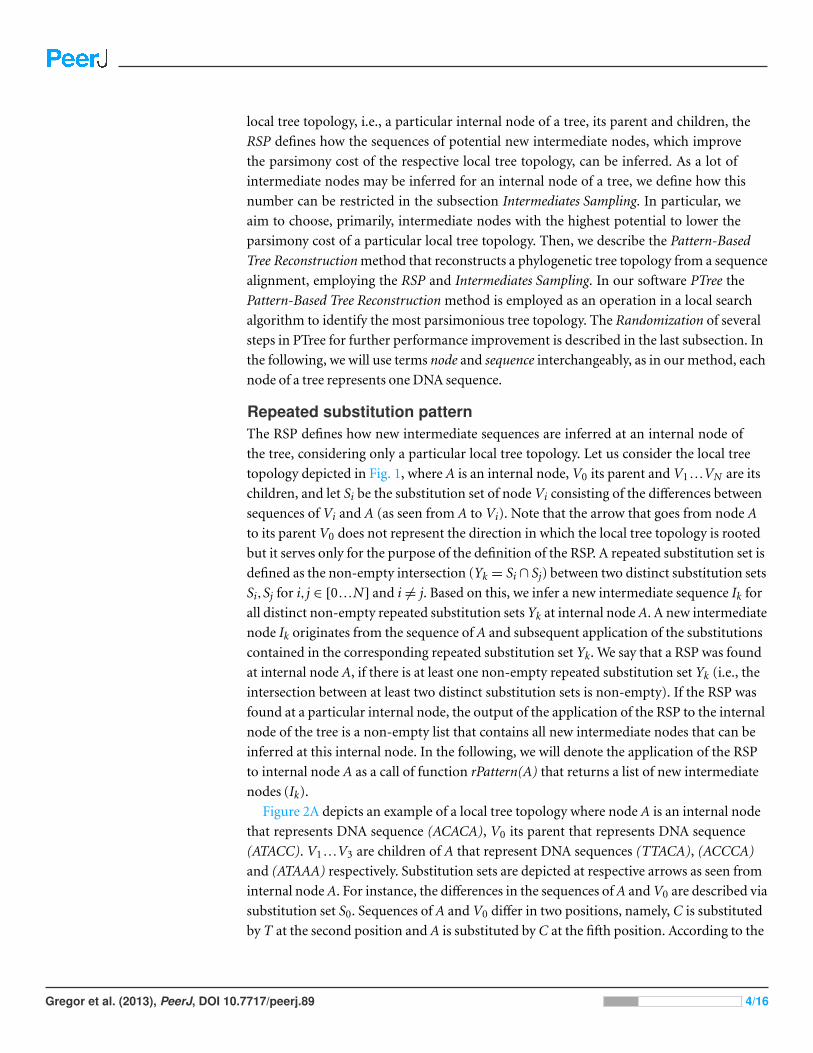
Figure 2A depicts an example of a local tree topology where node A is an internal node

that represents DNA sequence (ACACA), V0 its parent that represents DNA sequence

(ATACC). V1 ...V3 are children of A that represent DNA sequences (TTACA), (ACCCA)

and (ATAAA) respectively. Substitution sets are depicted at respective arrows as seen from

internal node A. For instance, the differences in the sequences of A and V0 are described via

substitution set S0. Sequences of A and V0 differ in two positions, namely, C is substituted

by T at the second position and A is substituted by C at the fifth position. According to the

Gregor et al. (2013), PeerJ, DOI 10.7717/peerj.89 4/16

Figure 1 Local tree topology. A is an internal node, V0 its parent, V1 ...VN are its children, and Sirepresents the corresponding substitution sets.

definition of the RSP, we can see that the intersection of at least two substitution sets (with

distinct indices) is non-empty, namely S0∩ S1 = S0∩ S3 = S1∩ S3 = {C2T} = Y1. Thus, we

can create a sequence of intermediate node I1, such that we apply the mutations in the in-

tersection set Y1 = {C2T} to the DNA sequence of node A(ACACA), which results in inter-

mediate sequence I1(ATACA), i.e., rPattern(A) returns a list of length one that contains I1.

Figure 2B depicts an expected local tree topology after node I1 is added. After the new

internal node I1 is added to the local tree topology, its cost decreases from 7 to 5. Thus, the

application of the RSP enables the inference of new intermediate nodes that can refine the

overall tree topology.

Intermediates samplingAs the application of the RSP, i.e., application of the function rPattern(A) to an internal

node A of degree n may produce up to n(n− 1)/2 intermediate nodes, we restrict the

number of intermediate nodes that can be inferred for a particular internal node with a

two-step procedure.

Step 1. We define the maximum number of intermediate nodes that can be in-

ferred at some internal node as a function of the degree of an internal node: F(n) =

max(round(c1 n),c2) where c1 and c2 are fixed coefficients (e.g., c1 = 4.0 and c2 = 1).

The purpose of this function is to allow the inference of more intermediate nodes at

internal nodes of higher degree. Let IA be the set of intermediate nodes that can be

inferred at internal node A (i.e., IA := rPattern(A)) and M := F(degree of A). To restrict

|IA| (i.e., the number of intermediate nodes that will be inferred at A), we choose at

Gregor et al. (2013), PeerJ, DOI 10.7717/peerj.89 5/16

Figure 2 Repeated substitution pattern example. (A) depicts a local tree topology where node A is aninternal node that represents DNA sequence (ACACA), V0 its parent, V1 ...V3 its children, and S0 ...S3are corresponding substitution sets. The repeated substitution pattern is found at node A since the inter-section of at least two substitution sets is non-empty, namely: S0∩ S1 = S0∩ S3 = S1∩ S3= {C2T} = Y1.Thus, new candidate intermediate node I1 (ATACA) originates from A (ACACA) by applying mutationsin Y1= {C2T}. Note that the arrow that goes from node A to its parent V0 does not represent the directionin which the local tree topology is rooted but it serves only for the purpose of the definition of the repeatedsubstitution pattern. (B) depicts an expected local tree topology after intermediate node I1 is added tothe tree topology. After I1 is added, the cost of the local tree topology (i.e., the number of substitutions)decreases from 7 to 5.

most M intermediate nodes out of IA with the biggest cost decrease, i.e., we compute

for each intermediate node from IA the cost decrease if a node was included in the local tree

topology regardless of the other candidate intermediate sequences. For instance, the cost

decrease after node I1 is included in the local tree topology in Fig. 2 is two. Note that we

perform the choice of intermediate nodes at random if we have more options for how to

choose intermediate nodes with the biggest cost decrease. Given IA, let us denote the set of

at most M intermediate nodes with the biggest cost decrease selected in this step as IA s1.

Gregor et al. (2013), PeerJ, DOI 10.7717/peerj.89 6/16

Step 2. Given IA s1, the intermediate nodes selected in the first step, the corresponding

internal node A, and its parent and children, we apply the following procedure:

(1) Compute the distance matrix (DM) based on pairwise evolutionary distances among

the sequences.

(2) Compute the minimum spanning tree (MST) based on the DM.

(3) Remove intermediate nodes of degree one or two.

(4) Repeat steps (1) to (4) until no intermediate nodes can be removed in step (3).

(5) Return the list of intermediate nodes that remain in the MST; let us denote this list as

IA s2.

In the following, we will denote the application of intermediates sampling as a call

of function iSample with a list of intermediate nodes and a respective internal node as

its arguments. Thus, iSample(rPattern(A), A) is a list of restricted size IA s2 that contains

intermediate nodes with the highest potential to lower the parsimony cost of the local tree

topology defined at internal node A.

Pattern-based tree reconstructionThis method reconstructs a tree topology from a given sequence alignment that can

represent both original input sequences that represent, for example, species, and the

corresponding inferred intermediate ancestral sequences, where the latter are auxiliary

and optional. Let seqSet be the set of the aligned input sequences. The method comprises

seven steps:

(1) Initialize the distance matrix (DM), i.e., compute a neighbor-joining (NJ) tree based

on pairwise evolutionary distances among the given input sequences seqSet. Set the

DM to the path metric representing the distances in the inferred NJ tree, such that

for each pair of the input sequences (i.e., leaf nodes of the NJ tree), the DM contains

an entry that specifies their distance in the NJ tree. Here, we initialize the DM for

the consequent minimum spanning tree (MST) computation in this way, since we

observed that our method yields better results than if we computed the MST only

based on the pairwise number of differences among the input sequences.

(2) Compute an MST from the DM. The MST represents a tree with the lowest cost

considering only the given input sequences seqSet. The MST is an approximation

of a minimum Steiner tree (Hwang, Richards & Winter, 1992); therefore it is a good

starting point for the intermediate inference, in which we further improve the tree

topology (i.e., lower its overall parsimony cost) by adding new intermediate nodes.

(3) Infer new candidate intermediate sequences based on the RSPs. Note that a candidate

intermediate sequence denotes a sequence that can be added to the tree topology,

while an intermediate sequence refers to a sequence that has been added to the current

tree topology. All candidate intermediate sequences, inferred at this step, are collected

by the depth-first search (DFS) algorithm, which efficiently traverses the whole tree

and visits all internal nodes to identify RSPs. Thus, we get the list of all candidate

Gregor et al. (2013), PeerJ, DOI 10.7717/peerj.89 7/16

intermediate sequences cSeq by calling function iSample(rPattern(A), A) for each

internal node A of the tree and by concatenating the resulting lists. More precisely,

new candidate intermediate sequences are inferred under consideration of a particular

local tree topology, consisting of an arbitrary internal node, its parent, and its children.

New candidate intermediate sequences are inferred if a RSP can be found for this local

tree topology. Intermediates sampling, the two-step approach, is then employed to

get only a restricted number of candidate intermediate nodes at a particular internal

node. After all new candidate intermediate sequences have been collected, we remove

duplicate candidate intermediate sequences from cSeq (duplicates to each other, or

to sequences represented by nodes in the current tree, i.e., in seqSet). Note that

inferred intermediate sequences are subsequently added to the sequence set for the

tree inference, and can be placed as either internal or leaf nodes in the subsequent

tree inference steps. Therefore, the inference of new intermediate sequences plays an

important role.

(4) Merge the new candidate intermediate sequences cSeq, inferred in the previous step,

with all sequences from the current tree seqSet. Let seqSet be the merged set. Iteratively

recompute the distance matrix (DM), i.e., set the entries of the DM to specify the

number of different characters between each pair of sequences from seqSet, recompute

the MST according to the DM and remove intermediate nodes of degree one (i.e., leaf

nodes) or two (superfluous internal nodes), as they are uninformative, until no

(candidate) intermediate sequence can be removed. Note that the corresponding

sequences are also removed from seqSet. The candidate intermediate sequences that

remain in the current tree after this step become intermediate sequences and seqSet

contains all sequences of the nodes of the current tree.

(5) Repeat steps (2) to (5) until no new candidate intermediate sequences can be found in

step (3).

(6) For each internal node that represents an original input sequence (e.g., existing

species), create a copy of the node and place it as a child node of the respective

internal node that represents the same sequence, so that all original input sequences are

represented by leaf nodes of the resulting tree.

(7) Return the resulting phylogenetic tree topology.

Let us denote the application of this pattern-based tree reconstruction method to the set

of input sequences seqSet as a call of function pbTree(seqSet) that returns a tree topology.

PTreeOur software PTree employs the pattern-based tree reconstruction method as an operation

in a local search for the most parsimonious tree topology. PTree searches for an optimal

solution to the maximum parsimony problem by traversing the tree space of feasible

solutions and keeping only the last feasible solution with the lowest parsimony cost that has

been found so far.

In addition to the set of aligned input genetic sequences seqSet, PTree requires

specification of the parameters d, b and k: The parameter d denotes the percentages of

Gregor et al. (2013), PeerJ, DOI 10.7717/peerj.89 8/16

internal nodes to be deleted from the tree. To allow refinement of the tree topology, the

search for the most parsimonious tree topology cannot terminate before b iterations

overall (the burn-in phase) and before k iterations where no more parsimonious tree

relative to the best tree found so far has been observed. For our experiments, we set d to

10%, b to 100 and k to 10.

PTree operates in three steps:

(1) The algorithm initializes the search with a neighbor-joining (NJ) tree inferred from

the input sequence alignment seqSet. We set the currentTree to be this NJ tree. In

PTree, we have incorporated a relaxed neighbor-joining algorithm with computational

complexity O(N2logN) (Sheneman, Evans & Foster, 2006). Distance corrections based

on the Jukes–Cantor (Jukes & Cantor, 1969) or the Kimura two-parameter model

(Kimura, 1980) that are available in this implementation can optionally be performed,

however, in our experiments we found no notable differences in results with different

evolutionary models.

(2) Updating the current tree topology, i.e., delete d% of randomly chosen internal

nodes from the currentTree and return rSeq, the set of sequences associated with

remaining nodes (internal and leaf nodes). The set rSeq is passed to our pattern-based

tree reconstruction method, i.e., the function pbTree(rSeq) returns a newTree. If the

newTree has a lower parsimony cost than the currentTree, the newTree becomes the

currentTree; else, the currentTree remains the same as it was.

(3) Repeat steps (2) and (3) until the number of iterations is larger than b and no update

of the currentTree has been performed for the last k iterations. Then, return the

currentTree as the final phylogenetic tree.

RandomizationRandomization of some steps of our method substantially improves its accuracy. The

MST algorithm, the NJ algorithm and the intermediates sampling are randomized. Since

some edges of a graph can have the same weights and any of these edges can be added at

a particular step of an MST algorithm, the MST is not unequivocally defined. Standard

implementations of the MST algorithm usually return the same tree after two consecutive

runs with the same input. Thus, we have modified the MST algorithm so that it is likely

that two consecutive runs produce two different tree topologies with the same cost, using

the same input sequences. At the point where the MST algorithm can add several distinct

edges with the same cost (weight) to the current graph, it decides at random which edge

will be added. There can be more options for choosing two clusters that will be merged at a

particular step of an NJ algorithm, and thus the resulting NJ tree is also not unequivocally

defined; therefore, we have employed a randomized version of the relaxed NJ algorithm

(Sheneman, Evans & Foster, 2006). Different MST topologies facilitate inference of more

various candidate intermediate sequences, which leads to better accuracy of the resulting

phylogenetic trees, since we also explore the larger neighborhood of the current trees in the

local search.

Gregor et al. (2013), PeerJ, DOI 10.7717/peerj.89 9/16

RESULTSTo validate the performance of PTree, we compared it with widely used methods on

reference datasets of PhyML (Guindon & Gascuel, 2003) and RAxML (Stamatakis, Ludwig

& Meier, 2005), as well as on alignments of concatenated Human Immunodeficiency

Virus (HIV) reverse transcriptase and polymerase sequences from EuResist (2010). We

tested for topological accuracy, cost optimality and runtime. All computations were done

on a machine with 2.8 GHz Dual-Core AMD Opteron Processor 8820. The Java Virtual

Machine was given 4GB of the main memory for the datasets up to 4,000 taxa and 8GB for

the datasets of 8,000 taxa, and all programs were run in a single thread.

Topological accuracyTests for topological accuracy were done in accordance to PhyML (Guindon & Gascuel,

2003) on 5,000 datasets with known topology where each dataset contained 40 taxa of

500bp length each. To compare the true and the reconstructed tree topologies, we used

the Robinson-Foulds distance (Robinson & Foulds, 1981), although this measure is more

conservative than other measures such as SPR or TBR, we chose it to allow a comparison

with results shown for PhyML in Guindon & Gascuel (2003). Reference methods were

PAUP* NJ, PAUP* maximum parsimony (with the TBR branch swapping option used in

the heuristic search), PAUP* maximum likelihood (with the NNI branch swapping option

used in the heuristic search), PhyML and TNT (with the SPR branch swapping option used

in the heuristic search). The results are depicted in Fig. 3. As expected, the best results in

terms of the Robinson–Foulds distance (Robinson & Foulds, 1981) between the inferred

and true tree topology were achieved by the maximum likelihood methods, followed

by the parsimony methods (including PTree). The worst results were yielded by NJ, the

representative of a distance-based method. Furthermore, within the parsimony methods,

PTree outperforms PAUP* used with the tree bisection and reconnection (TBR) heuristic,

which is the most extensive and accurate search heuristic.

Cost optimality and runtimeTo assess the performance of PTree in terms of parsimony costs and runtime, we compared

it with PAUP* NNI, SPR, TBR and TNT SPR heuristics on the reference datasets of

RAxML, as well as on a dataset of HIV reverse transcriptase and polymerase sequences. For

each dataset, we created seven subsets of different size (125–8,000 sequences). Sequences

of the HIV datasets were ∼1,600bp in length and the sequences of the RAxML datasets

were∼1,200bp. For the RAxML subsets, we took the arb 10000 dataset, selected the first

8,000 sequences and then subsequently selected the first half of the remaining sequences

for a new dataset. The HIV subsets were created in a similar fashion: we downloaded

∼8,000 reverse transcriptase and polymerase sequences from EuResist (2010), aligned

them and repeatedly selected the first half of the remaining sequences as a new dataset.

As two consecutive runs of PAUP* (NNI, SPR, or TBR) or PTree can result in different

results, we identified the mean (average over multiple runs), minimum, and maximum

parsimony costs and runtimes. Thus, PAUP* was run six times (except for the tests with

the SPR and TBR heuristics with the RAxML dataset with 4,000 sequences that were run

Gregor et al. (2013), PeerJ, DOI 10.7717/peerj.89 10/16

Figure 3 Topological accuracy. Comparison of topological accuracies of selected tree building methodsas a function of sequence divergence using 5,000 datasets of 40 taxa with 500 bases each from Guindon &Gascuel (2003). PTree was run with 50 iterations and Jukes–Cantor correction enabled. PAUP* was runwith the following settings: Neighbor Joining (NJ), maximum parsimony (MP; with the tree bisectionand reconnection (TBR) branch swapping option used in the heuristic search), and maximum likelihood(ML; with the nearest neighbor interchange (NNI) branch swapping option used in the heuristic search).TNT was run with the subtree pruning and regrafting (SPR) branch swapping option used in the heuristicsearch.

just once; the test with the TBR heuristic with the RAxML dataset with 2,000 sequences

that was run twice; and the test with the TBR heuristic with the HIV dataset with 4,000

sequences that was run twice as well); PTree (run with 100 iterations and without distance

correction) was run 10 times for all datasets. Some tests were done with lower number of

runs due to the limited computational resources. The comparison of the resulting average

parsimony costs is shown in Tables 1 and 3, and the comparison of the corresponding

average runtimes is shown in Tables 2 and 4. The comparisons of the corresponding

minimum and maximum parsimony costs, as well as the comparison of the minimum and

maximum runtimes are shown in Tables S1–S8. Furthermore, to enable the comparison

of different methods proportionally to the resulting parsimony costs and runtimes of

PTree, Tables S9–S20 show the results of Tables 1–4 and Tables S1–S8, respectively, in terms

of percentages. In terms of the average values, PTree outperforms PAUP* with the NNI

Gregor et al. (2013), PeerJ, DOI 10.7717/peerj.89 11/16

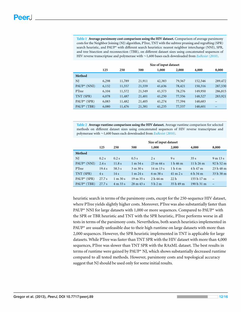
Table 1 Average parsimony cost comparison using the HIV dataset. Comparison of average parsimonycosts for the Neighbor Joining (NJ) algorithm, PTree, TNT with the subtree pruning and regrafting (SPR)search heuristic, and PAUP* with different search heuristics: nearest neighbor interchange (NNI), SPR,and tree bisection and reconnection (TBR), on different dataset sizes using concatenated sequences ofHIV reverse transcriptase and polymerase with∼1,600 bases each downloaded from EuResist (2010).

Size of input dataset

125 250 500 1,000 2,000 4,000 8,000

Method

NJ 6,298 11,789 21,911 42,383 79,567 152,546 289,472

PAUP* (NNI) 6,132 11,557 21,559 41,636 78,421 150,316 287,530

PTree 6,104 11,572 21,549 41,573 78,276 149,950 286,815

TNT (SPR) 6,078 11,487 21,401 41,250 77,556 148,527 283,921

PAUP* (SPR) 6,083 11,482 21,405 41,274 77,594 148,683 –

PAUP* (TBR) 6,080 11,476 21,381 41,235 77,537 148,601 –

Table 2 Average runtime comparison using the HIV dataset. Average runtime comparison for selectedmethods on different dataset sizes using concatenated sequences of HIV reverse transcriptase andpolymerase with∼1,600 bases each downloaded from EuResist (2010).

Size of input dataset

125 250 500 1,000 2,000 4,000 8,000

Method

NJ 0.2 s 0.2 s 0.5 s 2 s 9 s 35 s 9 m 13 s

PAUP* (NNI) 2.4 s 11.8 s 1 m 54 s 23 m 44 s 1 h 46 m 11 h 26 m 92 h 52 m

PTree 19.4 s 58.5 s 3 m 30 s 14 m 13 s 1 h 4 m 4 h 47 m 23 h 48 m

TNT (SPR) 4 s 14 s 1 m 24 s 6 m 38 s 41 m 2 s 6 h 34 m 33 h 38 m

PAUP* (SPR) 27.7 s 1 m 30 s 19 m 35 s 2 h 44 m 22 h 155 h 17 m –

PAUP* (TBR) 27.7 s 4 m 33 s 28 m 43 s 5 h 2 m 35 h 49 m 190 h 31 m –

heuristic search in terms of the parsimony costs, except for the 250-sequence HIV dataset,

where PTree yields slightly higher costs. Moreover, PTree was also substantially faster than

PAUP* NNI for large datasets with 1,000 or more sequences. Compared to PAUP* with

the SPR or TBR heuristic and TNT with the SPR heuristic, PTree performs worse in all

tests in terms of the parsimony costs. Nevertheless, both search heuristics implemented in

PAUP* are usually unfeasible due to their high runtime on large datasets with more than

2,000 sequences. However, the SPR heuristic implemented in TNT is applicable for large

datasets. While PTree was faster than TNT SPR with the HIV dataset with more than 4,000

sequences, PTree was slower than TNT SPR with the RAxML dataset. The best results in

terms of runtime were gained by PAUP* NJ, which shows substantially decreased runtime

compared to all tested methods. However, parsimony costs and topological accuracy

suggest that NJ should be used only for some initial results.

Gregor et al. (2013), PeerJ, DOI 10.7717/peerj.89 12/16

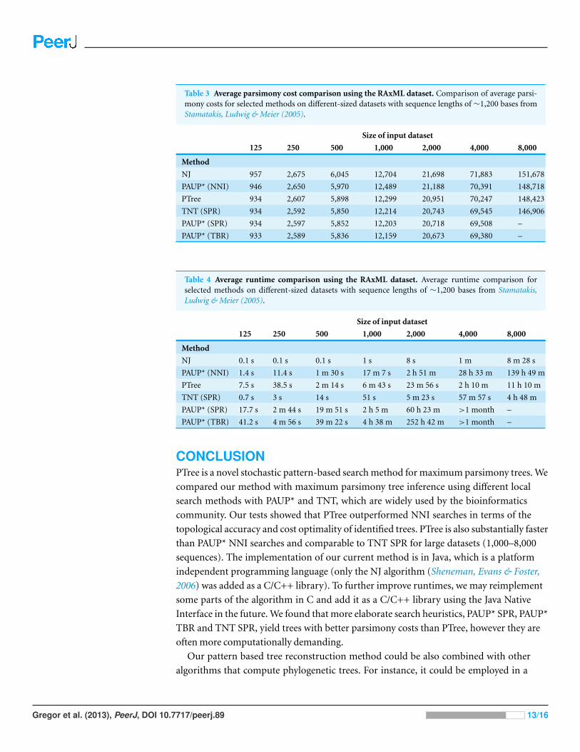
Table 3 Average parsimony cost comparison using the RAxML dataset. Comparison of average parsi-mony costs for selected methods on different-sized datasets with sequence lengths of ∼1,200 bases fromStamatakis, Ludwig & Meier (2005).

Size of input dataset

125 250 500 1,000 2,000 4,000 8,000

Method

NJ 957 2,675 6,045 12,704 21,698 71,883 151,678

PAUP* (NNI) 946 2,650 5,970 12,489 21,188 70,391 148,718

PTree 934 2,607 5,898 12,299 20,951 70,247 148,423

TNT (SPR) 934 2,592 5,850 12,214 20,743 69,545 146,906

PAUP* (SPR) 934 2,597 5,852 12,203 20,718 69,508 –

PAUP* (TBR) 933 2,589 5,836 12,159 20,673 69,380 –

Table 4 Average runtime comparison using the RAxML dataset. Average runtime comparison forselected methods on different-sized datasets with sequence lengths of ∼1,200 bases from Stamatakis,Ludwig & Meier (2005).

Size of input dataset

125 250 500 1,000 2,000 4,000 8,000

Method

NJ 0.1 s 0.1 s 0.1 s 1 s 8 s 1 m 8 m 28 s

PAUP* (NNI) 1.4 s 11.4 s 1 m 30 s 17 m 7 s 2 h 51 m 28 h 33 m 139 h 49 m

PTree 7.5 s 38.5 s 2 m 14 s 6 m 43 s 23 m 56 s 2 h 10 m 11 h 10 m

TNT (SPR) 0.7 s 3 s 14 s 51 s 5 m 23 s 57 m 57 s 4 h 48 m

PAUP* (SPR) 17.7 s 2 m 44 s 19 m 51 s 2 h 5 m 60 h 23 m >1 month –

PAUP* (TBR) 41.2 s 4 m 56 s 39 m 22 s 4 h 38 m 252 h 42 m >1 month –

CONCLUSIONPTree is a novel stochastic pattern-based search method for maximum parsimony trees. We

compared our method with maximum parsimony tree inference using different local

search methods with PAUP* and TNT, which are widely used by the bioinformatics

community. Our tests showed that PTree outperformed NNI searches in terms of the

topological accuracy and cost optimality of identified trees. PTree is also substantially faster

than PAUP* NNI searches and comparable to TNT SPR for large datasets (1,000–8,000

sequences). The implementation of our current method is in Java, which is a platform

independent programming language (only the NJ algorithm (Sheneman, Evans & Foster,

2006) was added as a C/C++ library). To further improve runtimes, we may reimplement

some parts of the algorithm in C and add it as a C/C++ library using the Java Native

Interface in the future. We found that more elaborate search heuristics, PAUP* SPR, PAUP*

TBR and TNT SPR, yield trees with better parsimony costs than PTree, however they are

often more computationally demanding.

Our pattern based tree reconstruction method could be also combined with other

algorithms that compute phylogenetic trees. For instance, it could be employed in a

Gregor et al. (2013), PeerJ, DOI 10.7717/peerj.89 13/16

memetic algorithm in several ways: as an operation in a local search algorithm, as

a mutation operator or as a recombination operator. To recombine two trees, the

pattern-based tree reconstruction method can be given all previously inferred internal

nodes of both trees and all original input sequences as an input, which results in a new tree.

Thus, our new pattern-based method enriches the set of current phylogeny reconstruction

tools and methods.

ADDITIONAL INFORMATION AND DECLARATIONS

FundingI.G., L.S. and A.C.M were funded by the Max-Planck Society and Heinrich-Heine

University Dusseldorf. The funders had no role in study design, data collection and

analysis, decision to publish, or preparation of the manuscript.

Grant DisclosuresThe following grant information was disclosed by the authors:

Max-Planck Society.

Heinrich-Heine-University Dusseldorf.

Competing InterestsAlice C. McHardy is an Academic Editor for PeerJ. All the authors declare no other

competing interests.

Author Contributions• Ivan Gregor and Lars Steinbruck performed the experiments, analyzed the data, wrote

the paper.

• Alice C. McHardy conceived and designed the experiments, analyzed the data, wrote the

paper.

Supplemental InformationSupplemental information for this article can be found online at http://dx.doi.org/

10.7717/peerj.89.

REFERENCESBenson DA, Karsch-Mizrachi I, Lipman DJ, Ostell J, Sayers EW. 2011. GenBank. Nucleic Acids

Research 39:32–37 DOI 10.1093/nar/gkq1079.

Carroll H, Teichert AR, Krein J, Sundberg K, Snell Q, Clement M. 2009. An open sourcephylogenetic search and alignment package. International Journal of Bioinformatics Researchand Applications 5:349–364 DOI 10.1504/IJBRA.2009.026424.

EuResist. 2010. HIV reverse transcriptase and polymerase sequences. Available athttp://www.euresist.org/web/guest (accessed 12 April 2010).

Felsenstein J. 1978. Cases in which parsimony or compatibility methods will be positivelymisleading. Systematic Zoology 27:401–410 DOI 10.2307/2412923.

Felsenstein J. 2003. Inferring phylogenies, 2nd ed. Sunderland: Sinauer Associates.

Gregor et al. (2013), PeerJ, DOI 10.7717/peerj.89 14/16

Felsenstein J. 2005. PHYLIP (phylogeny inference package) version 3.6. Seattle: Department ofGenome Sciences, University of Washington.

Fischer M. 2012. Non-hereditary maximum parsimony trees. Journal of Mathematical Biology65(2):293–308 DOI 10.1007/s00285-011-0458-9.

Goeffon A, Richer JM, Hao JK. 2008. Progressive tree neighborhood applied to the maximumparsimony problem. Transactions on Computational Biology and Bioinformatics 5:136–145DOI 10.1109/TCBB.2007.1065.

Goloboff PA, Catalano SA, Farris JS. 2009. Phylogenetic analysis of 73 060 taxa corroboratesmajor eukaryotic groups. Cladistics 25:211–230 DOI 10.1111/j.1096-0031.2009.00255.x.

Goloboff PA, Farris JS, Nixon KC. 2008. TNT, a free program for phylogenetic analysis. Cladistics24:774–786 DOI 10.1111/j.1096-0031.2008.00217.x.

Graham RL. 1982. The Steiner problem in phylogeny is NP-complete. Advances in AppliedMathematics 3:43–49 DOI 10.1016/S0196-8858(82)80004-3.

Guindon S, Gascuel O. 2003. A simple, fast, and accurate algorithm to estimate large phylogeniesby maximum likelihood. Systematic Biology 52:696–704 DOI 10.1080/10635150390235520.

Hill T, Lundgren A, Fredriksson R, Schioth HB. 2005. Genetic algorithm for large-scalemaximum parsimony phylogenetic analysis of proteins. Biochimica et Biophysica Acta1725:19–29 DOI 10.1016/j.bbagen.2005.04.027.

Huelsenbeck JP, Ronquist F. 2001. MRBAYES: bayesian inference of phylogenetic trees.Bioinformatics 17:754–755 DOI 10.1093/bioinformatics/17.8.754.

Hwang FK, Richards DS, Winter P. 1992. The Steiner tree problem, Annals of Discrete Mathematics53. North-Holland: Elsevier.

Jukes TH, Cantor CR. 1969. Evolution of protein molecules. In: Munro HN, ed. Mammalianprotein metabolism 3. NY: Academic Press, 21–132.

Kasap S, Benkrid K. 2011. High performance phylogenetic analysis with maximumparsimony on reconfigurable hardware. Very Large Scale Integration Systems 19:796–808DOI 10.1109/TVLSI.2009.2039588.

Kimura M. 1980. A simple method for estimating evolutionary rates of base substitutionsthrough comparative studies of nucleotide sequences. Journal of Molecular Evolution 16:111–120DOI 10.1007/BF01731581.

Kuck P, Mayer C, Wagele JW, Misof B. 2012. Long branch effects distort maximum likelihoodphylogenies in simulations despite selection of the correct model. PLoS ONE 7(5):e36593DOI 10.1371/journal.pone.0036593.

McHardy AC, Adams B. 2009. The role of genomics in tracking the evolution of influenza A virus.PLoS Pathogens 5:1–6 DOI 10.1371/journal.ppat.1000566.

Metzker ML. 2010. Sequencing technologies — the next generation. Nature Reviews: Genetics11:31–46 DOI 10.1038/nrg2626.

Ribeiro CC, Vianna DS. 2005. A GRASP/VND heuristic for the phylogeny problem using anew neighborhood structure. International Transactions in Operational Research 12:325–338DOI 10.1111/j.1475-3995.2005.498 1.x.

Richer JM, Goeffon A, Hao JK. 2009. A memetic algorithm for phylogenetic reconstructionwith maximum parsimony. In: EvoBIO ’09 proceedings of the 7th European conference onevolutionary computation. Machine Learning and Data Mining in Bioinformatics 164–175DOI 10.1007/978-3-642-01184-9 15.

Gregor et al. (2013), PeerJ, DOI 10.7717/peerj.89 15/16

Robinson DF, Foulds LR. 1981. Comparison of phylogenetic trees. Mathematical Biosciences53:131–147 DOI 10.1016/0025-5564(81)90043-2.

Russell CA, Jones TC, Barr IG, Cox NJ, Garten RJ, Gregory V, Gust ID, Hampson AW, Hay AJ,Hurt AC, de Jong JC, Kelso A, Klimov AI, Kageyama T, Komadina N, Lapedes AS, Lin YP,Mosterin A, Obuchi M, Odagiri T, Osterhaus ADME, Rimmelzwaan GF, Shaw MW,Skepner E, Stohr K, Tashiro M, Fouchier RAM, Smith DJ. 2008. Influenza vaccine strainselection and recent studies on the global migration of seasonal influenza viruses. Vaccine26:31–34 DOI 10.1016/j.vaccine.2008.07.078.

Saitou N, Nei M. 1987. The neighbor-joining method: a new method for reconstructingphylogenetic trees. Molecular Biology and Evolution 4:406–425.

Sanderson MJ. 2007. Construction and annotation of large phylogenetic trees. AustralianSystematic Botany 20:287–301 DOI 10.1071/SB07006.

Sheneman L, Evans J, Foster JA. 2006. Clearcut: a fast implementation of relaxed neighbor joining.Bioinformatics 22:2823–2824 DOI 10.1093/bioinformatics/btl478.

Sokal RR, Michener CD. 1958. A statistical method for evaluating systematic relationships. TheUniversity of Kansas Science Bulletin 38:1409–1438.

Stamatakis A, Ludwig T, Meier H. 2005. RAxML-III: a fast program for maximumlikelihood-based inference of large phylogenetic trees. Bioinformatics 21:456–463DOI 10.1093/bioinformatics/bti191.

Steel M, Penny D. 2000. Parsimony, likelihood, and the role of models in molecular phylogenetics.Molecular Biology and Evolution 17:839–850 DOI 10.1093/oxfordjournals.molbev.a026364.

Sundberg K, O’Connor T, Carroll H, Clement M, Snell Q. 2008. Parsimony acceleratedmaximum likelihood searches. International Journal of Computational Biology and Drug Design1:74–87 DOI 10.1504/IJCBDD.2008.018711.

Swofford DL. 2002. PAUP*: phylogenetic analysis using parsimony (* and other methods), version 4.Sunderland: Sinauer Associates.

Tamura K, Peterson D, Peterson N, Stecher G, Nei M, Kumar S. 2011. MEGA5: molecularevolutionary genetics analysis using maximum likelihood, evolutionary distance,and maximum parsimony methods. Molecular Biology and Evolution 28:2731–2739DOI 10.1093/molbev/msr121.

Varon A, Vinh LS, Wheeler WC. 2010. POY version 4: phylogenetic analysis using dynamichomologies. Cladistics 26:72–85 DOI 10.1111/j.1096-0031.2009.00282.x.

White WTJ, Holland BR. 2011. Faster exact maximum parsimony search with XMP.Bioinformatics 27:1359–1367 DOI 10.1093/bioinformatics/btr147.

Zwickl DJ. 2006. Genetic algorithm approaches for the phylogenetic analysis of large biologicalsequence datasets under the maximum likelihood criterion. D. Phil. Thesis, University of Texas.

Gregor et al. (2013), PeerJ, DOI 10.7717/peerj.89 16/16