Embed Size (px)
Citation preview

PATH PLANNINGPATH PLANNING
Presented by : Mohamadreza NegahdarPresented by : Mohamadreza Negahdar
Supervisor : Dr. AhmadianSupervisor : Dr. Ahmadian
Co-Supervisor : Prof. NavabCo-Supervisor : Prof. Navab
Tehran University of Medical SciencesTehran University of Medical Sciences
October 5 , 2005October 5 , 2005
OUTLINEOUTLINE
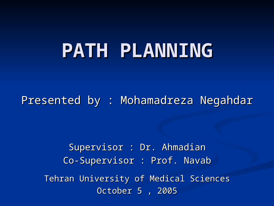
IntroductionIntroduction Path planning in medicinePath planning in medicine Automatic path generationAutomatic path generation Skeleton & skeletonizationSkeleton & skeletonization Skeletonization techniquesSkeletonization techniques Medical applicationsMedical applications Path planningPath planning
RoadmapRoadmap Cell decompositionCell decomposition Potential fieldPotential field
Virtual endoscopyVirtual endoscopy NavigationNavigation ApplicationsApplications Our workOur work
IntroductionIntroduction
How can “see” inside the body to screen and How can “see” inside the body to screen and cure?cure?
Centerline extraction is the basis to understand Centerline extraction is the basis to understand three dimensional structure of the organthree dimensional structure of the organ
Given a map and goal location, identify Given a map and goal location, identify trajectory to reach goal locationtrajectory to reach goal location
Strategic competenceStrategic competence
How do we combine these two competencies, How do we combine these two competencies, along with localization, and mapping, into a along with localization, and mapping, into a coherent framework?coherent framework?
Path Planning in medicinePath Planning in medicine
Fly-through and navigationFly-through and navigation
General idea of the shape of the organ wallsGeneral idea of the shape of the organ walls
Detect an abnormal shapeDetect an abnormal shape
Making measurements for locating Making measurements for locating abnormalitiesabnormalities
Computing local distension and lengthComputing local distension and length
Risk of infection or perforation of the Risk of infection or perforation of the anatomy being examined will be eliminated anatomy being examined will be eliminated
Path Planning in medicinePath Planning in medicine
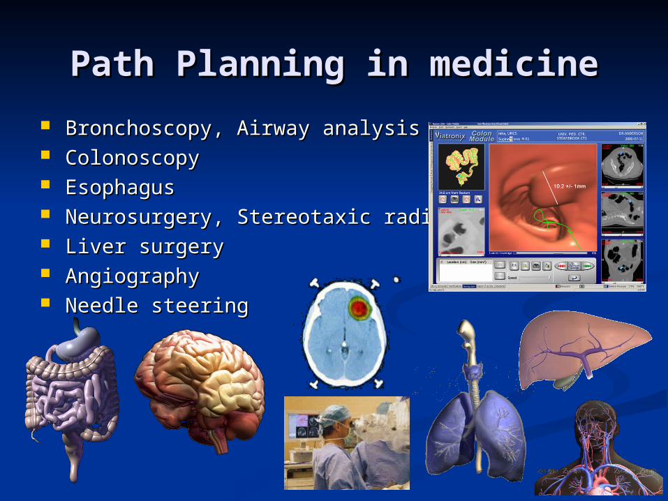
Bronchoscopy, Airway analysisBronchoscopy, Airway analysis ColonoscopyColonoscopy EsophagusEsophagus Neurosurgery, Stereotaxic radiosurgeryNeurosurgery, Stereotaxic radiosurgery Liver surgeryLiver surgery AngiographyAngiography Needle steeringNeedle steering
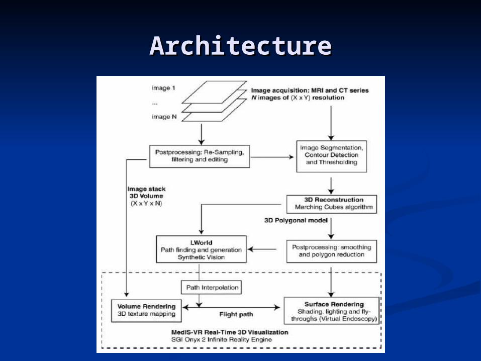
ArchitectureArchitecture
Restrictions of manually path Restrictions of manually path planningplanning
Very time consumingVery time consuming
Frustrating for a novice userFrustrating for a novice user
Need to improve the performance and Need to improve the performance and lower the costlower the cost
For this reason, we provide the surgeon For this reason, we provide the surgeon with an with an automatic path generationautomatic path generation..
Automatic Path GenerationAutomatic Path Generation
Surgeon loads a 3D modelSurgeon loads a 3D model
Defines a start and an end pointDefines a start and an end point
Program returns an optimal path centered Program returns an optimal path centered inside the modelinside the model
The user can fly-through the path and/or The user can fly-through the path and/or edit it manuallyedit it manually
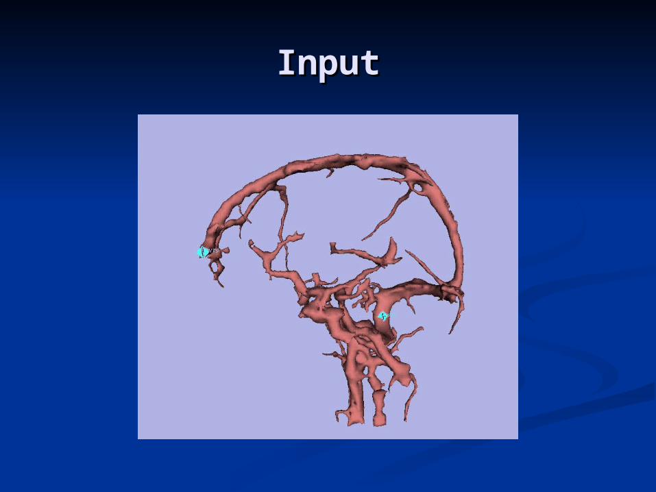
InputInput
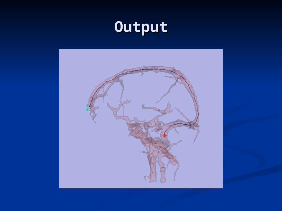
OutputOutput
Automatic Path Planning for Automatic Path Planning for VEVE
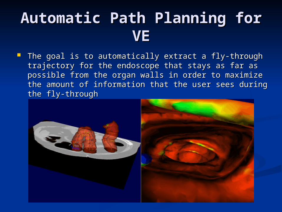
The goal is to automatically extract a fly-through trajectory The goal is to automatically extract a fly-through trajectory for the endoscope that stays as far as possible from the for the endoscope that stays as far as possible from the organ walls in order to maximize the amount of information organ walls in order to maximize the amount of information that the user sees during the fly-throughthat the user sees during the fly-through
SkeletonizationSkeletonization
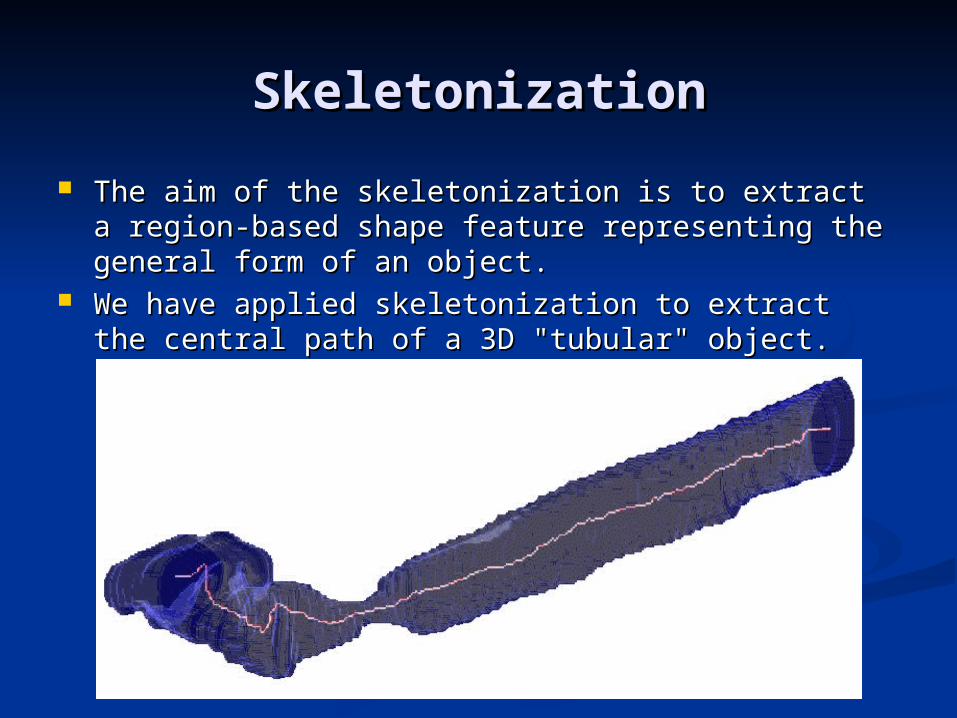
The aim of the skeletonization is to extract a region-The aim of the skeletonization is to extract a region-based shape feature representing the general form of based shape feature representing the general form of an object. an object.
We have applied skeletonization to extract the central We have applied skeletonization to extract the central path of a 3D "tubular" object.path of a 3D "tubular" object.
Skeleton of objectSkeleton of object
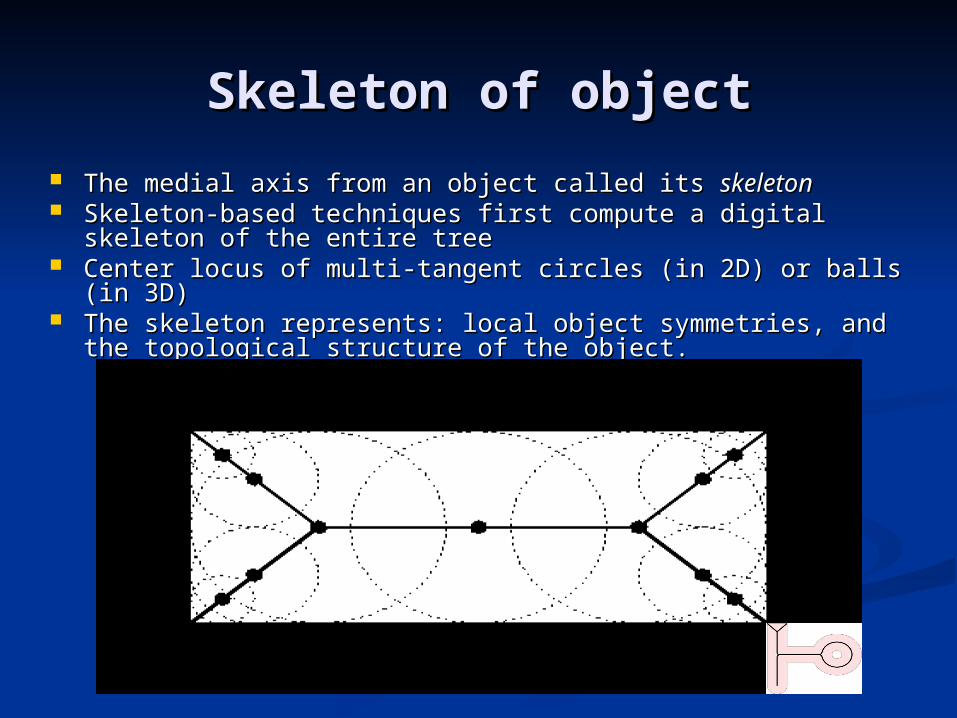
The medial axis from an object called its The medial axis from an object called its skeletonskeleton Skeleton-based techniques first compute a digital skeleton of Skeleton-based techniques first compute a digital skeleton of
the entire tree the entire tree Center locus of multi-tangent circles (in 2D) or balls (in 3D) Center locus of multi-tangent circles (in 2D) or balls (in 3D) The skeleton represents: local object symmetries, and the The skeleton represents: local object symmetries, and the
topological structure of the object. topological structure of the object.
Skeletonization techniquesSkeletonization techniques
detecting ridges in distance map of the detecting ridges in distance map of the boundary pointsboundary points
calculating the Voronoi diagram generated calculating the Voronoi diagram generated by the boundary pointsby the boundary points
the layer by layer erosion called thinningthe layer by layer erosion called thinning
Comparison of Skeletonization Comparison of Skeletonization TechniquesTechniques
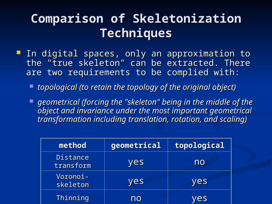
In digital spaces, only an approximation to the In digital spaces, only an approximation to the "true skeleton" can be extracted. There are two "true skeleton" can be extracted. There are two requirements to be complied with:requirements to be complied with:
topological (to retain the topology of the original topological (to retain the topology of the original object)object)
geometrical (forcing the "skeleton" being in the geometrical (forcing the "skeleton" being in the middle of the object and invariance under the most middle of the object and invariance under the most important geometrical transformation including important geometrical transformation including translation, rotation, and scaling)translation, rotation, and scaling)
methodmethod geometricalgeometrical topologicaltopological
Distance Distance transformtransform yesyes nono
Voronoi-skeletonVoronoi-skeleton yesyes yesyes
ThinningThinning nono yesyes
Distance TransformationDistance Transformation
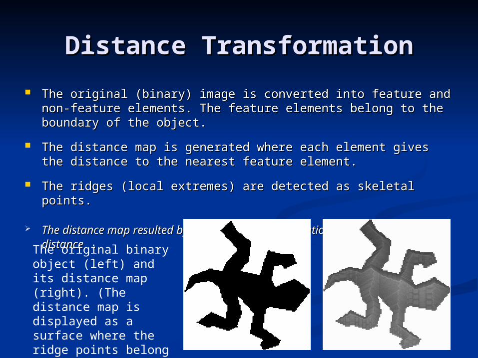
The original (binary) image is converted into feature and non-The original (binary) image is converted into feature and non-feature elements. The feature elements belong to the boundary feature elements. The feature elements belong to the boundary of the object.of the object.
The distance map is generated where each element gives the The distance map is generated where each element gives the distance to the nearest feature element.distance to the nearest feature element.
The ridges (local extremes) are detected as skeletal points. The ridges (local extremes) are detected as skeletal points.
The distance map resulted by the distance transformation depends The distance map resulted by the distance transformation depends on the chosen distanceon the chosen distance . .
The original binary object (left) and its distance map (right). (The distance map is displayed as a surface where the ridge points belong to the skeleton.)
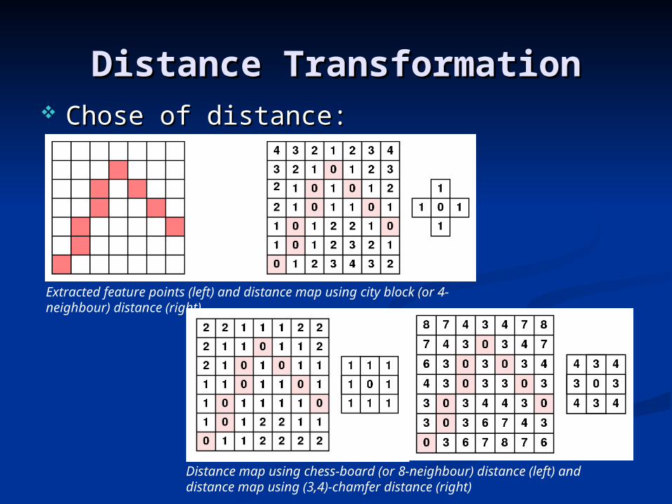
Distance TransformationDistance Transformation Chose of distance:Chose of distance:
Extracted feature points (left) and distance map using city block (or 4-neighbour) distance (right)
Distance map using chess-board (or 8-neighbour) distance (left) and distance map using (3,4)-chamfer distance (right)
Voronoi DiagramVoronoi Diagram
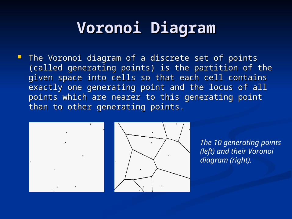
The Voronoi diagram of a discrete set of points (called The Voronoi diagram of a discrete set of points (called generating points) is the partition of the given space into generating points) is the partition of the given space into cells so that each cell contains exactly one generating point cells so that each cell contains exactly one generating point and the locus of all points which are nearer to this and the locus of all points which are nearer to this generating point than to other generating points.generating point than to other generating points.
The 10 generating points (left) and their Voronoi diagram (right).
Voronoi DiagramVoronoi Diagram
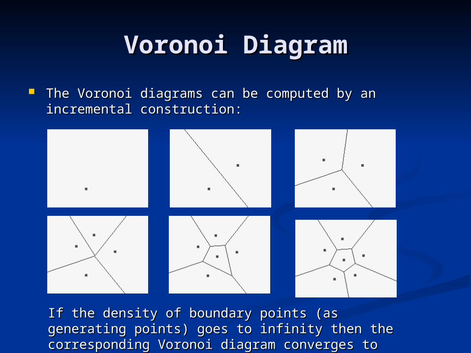
The Voronoi diagrams can be computed by an incremental The Voronoi diagrams can be computed by an incremental construction: construction:
If the density of boundary points (as generating If the density of boundary points (as generating points) goes to infinity then the corresponding points) goes to infinity then the corresponding Voronoi diagram converges to the skeleton.Voronoi diagram converges to the skeleton.
Voronoi SkeletonVoronoi Skeleton
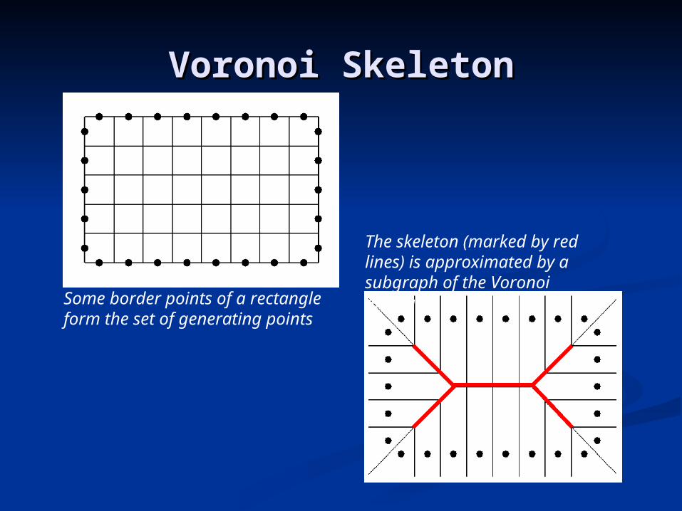
Some border points of a rectangle form the set of generating points
The skeleton (marked by red lines) is approximated by a subgraph of the Voronoi diagram
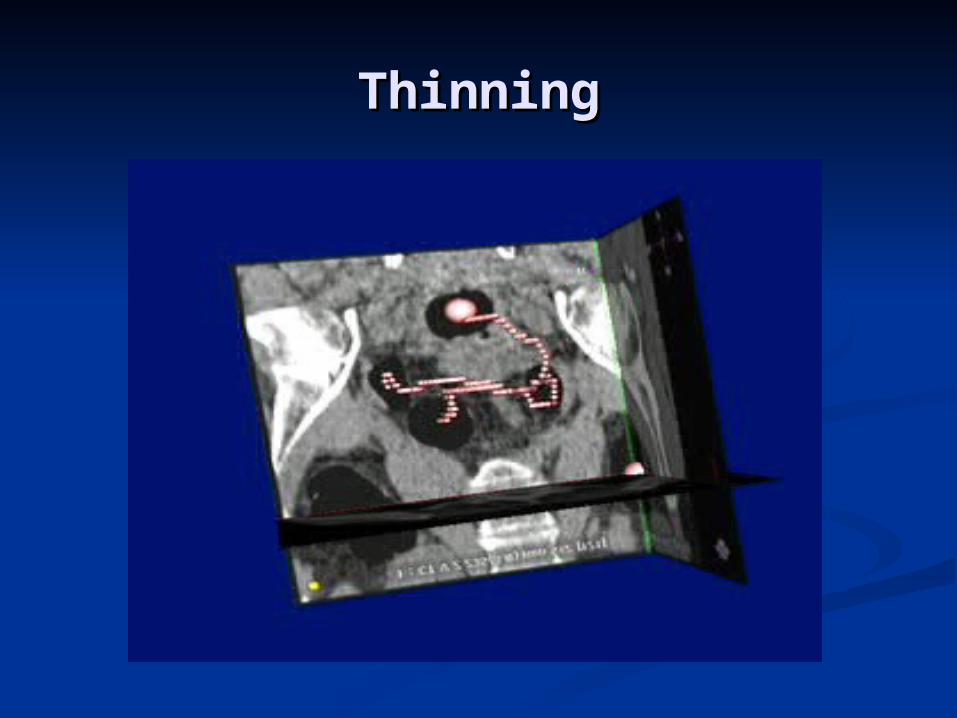
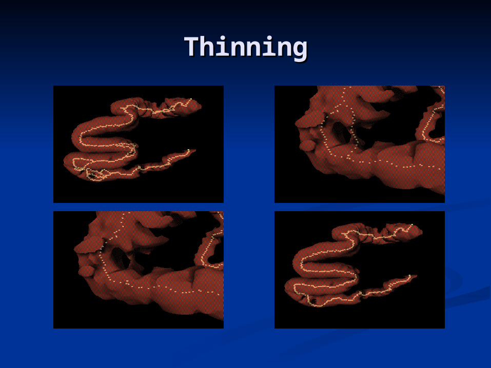
ThinningThinning
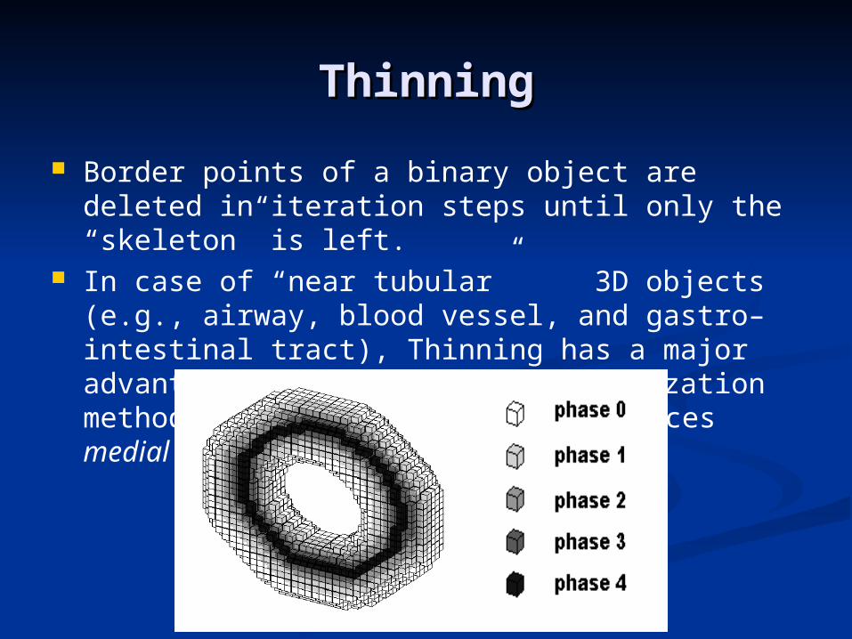
Border points of a binary object are deleted in iteration steps until only the “skeleton” is left.
In case of “near tubular” 3D objects (e.g., airway, blood vessel, and gastro–intestinal tract), Thinning has a major advantage over the other skeletonization methods since curve thinning can produces medial lines easily
ThinningThinning
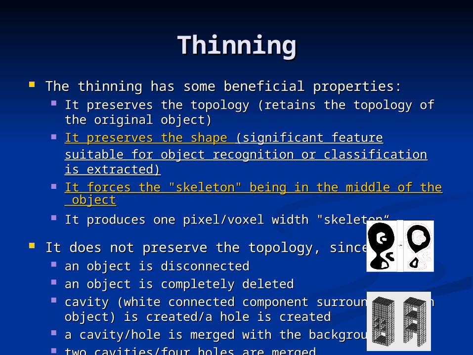
ThinningThinning The thinning has some beneficial properties:The thinning has some beneficial properties:
It preserves the topology (retains the topology of the It preserves the topology (retains the topology of the original object)original object)
It preserves the shape It preserves the shape (significant feature suitable for (significant feature suitable for object recognition or classification is extracted)object recognition or classification is extracted)
It forces the "skeleton" being in the middle of the objectIt forces the "skeleton" being in the middle of the object It produces one pixel/voxel width "skeleton“It produces one pixel/voxel width "skeleton“
It does not preserve the topology, sinceIt does not preserve the topology, since an object is disconnectedan object is disconnected an object is completely deletedan object is completely deleted cavity (white connected component surrounded by an cavity (white connected component surrounded by an
object) is created/a hole is createdobject) is created/a hole is created a cavity/hole is merged with the background a cavity/hole is merged with the background two cavities/four holes are merged two cavities/four holes are merged
ThinningThinning
Medical ApplicationsMedical Applications
assessment of laryngotracheal stenosisassessment of laryngotracheal stenosis
assessment of infrarenal aortic aneurysmassessment of infrarenal aortic aneurysm
unravelling the colonunravelling the colon
Each of the emerged three applications requires Each of the emerged three applications requires the cross-sectional profiles of the investigated the cross-sectional profiles of the investigated tubular organs tubular organs
ProcedureProcedure
image acquisition by Spiral Computed Tomography (S-CT)image acquisition by Spiral Computed Tomography (S-CT)
(semiautomatic snake-based) segmentation (i.e., (semiautomatic snake-based) segmentation (i.e., determining a binary object from the gray-level picturedetermining a binary object from the gray-level picture
morphological filtering of the segmented objectmorphological filtering of the segmented object
curve thinning (by using one of our 3D thinning algorithm)curve thinning (by using one of our 3D thinning algorithm)
raster-to-vector conversionraster-to-vector conversion
pruning the vector structure (i.e., removing the unwanted pruning the vector structure (i.e., removing the unwanted branches)branches)
smoothing the resulted central pathsmoothing the resulted central path
calculation of the cross-sectional profile orthogonal to the calculation of the cross-sectional profile orthogonal to the central pathcentral path
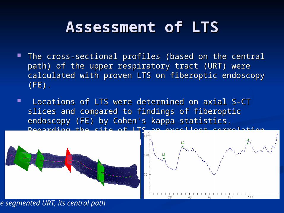
Assessment of LTSAssessment of LTS
The cross-sectional profiles (based on the central path) of The cross-sectional profiles (based on the central path) of the upper respiratory tract (URT) were calculated with the upper respiratory tract (URT) were calculated with proven LTS on fiberoptic endoscopy (FE).proven LTS on fiberoptic endoscopy (FE).
Locations of LTS were determined on axial S-CT slices and Locations of LTS were determined on axial S-CT slices and compared to findings of fiberoptic endoscopy (FE) by compared to findings of fiberoptic endoscopy (FE) by Cohen's kappa statistics. Regarding the site of LTS an Cohen's kappa statistics. Regarding the site of LTS an excellent correlation was found between FE and S-CT excellent correlation was found between FE and S-CT
(z=7.44, p<0.005).(z=7.44, p<0.005).
The segmented URT, its central path
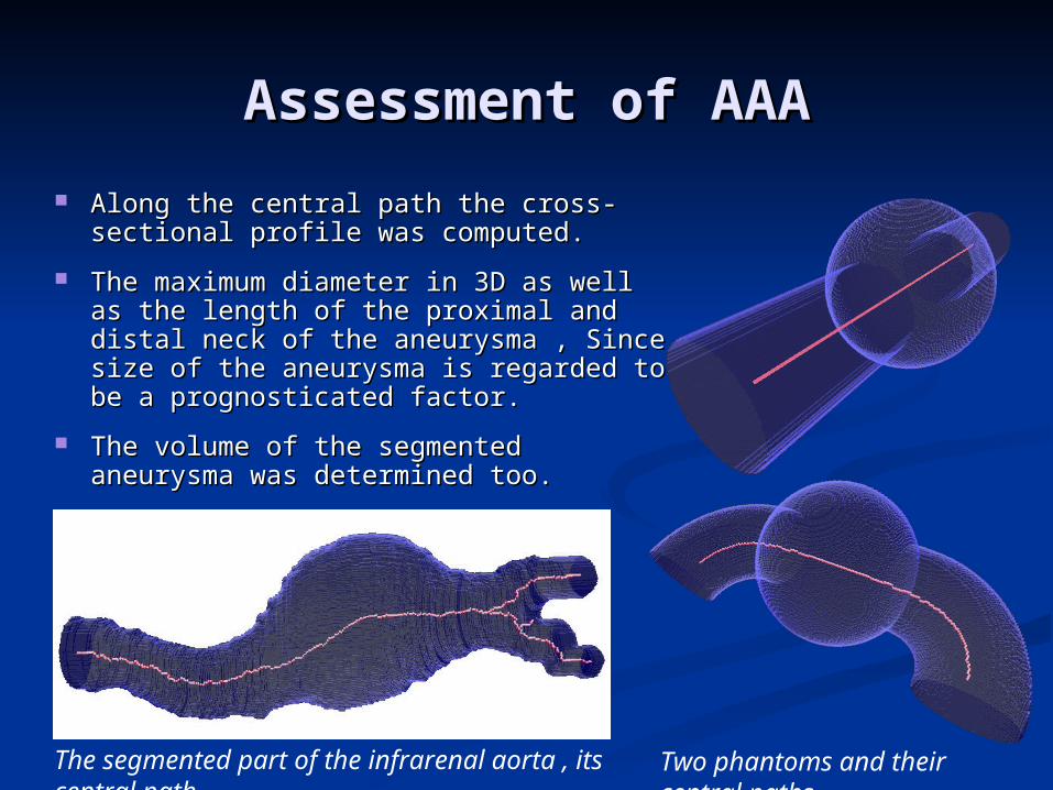
Assessment of AAAAssessment of AAA
Along the central path the cross-Along the central path the cross-sectional profile was computed.sectional profile was computed.
The maximum diameter in 3D as well The maximum diameter in 3D as well as the length of the proximal and as the length of the proximal and distal neck of the aneurysma , Since distal neck of the aneurysma , Since size of the aneurysma is regarded to size of the aneurysma is regarded to be a prognosticated factor.be a prognosticated factor.
The volume of the segmented The volume of the segmented aneurysma was determined too.aneurysma was determined too.
Two phantoms and their central paths
The segmented part of the infrarenal aorta , its central path
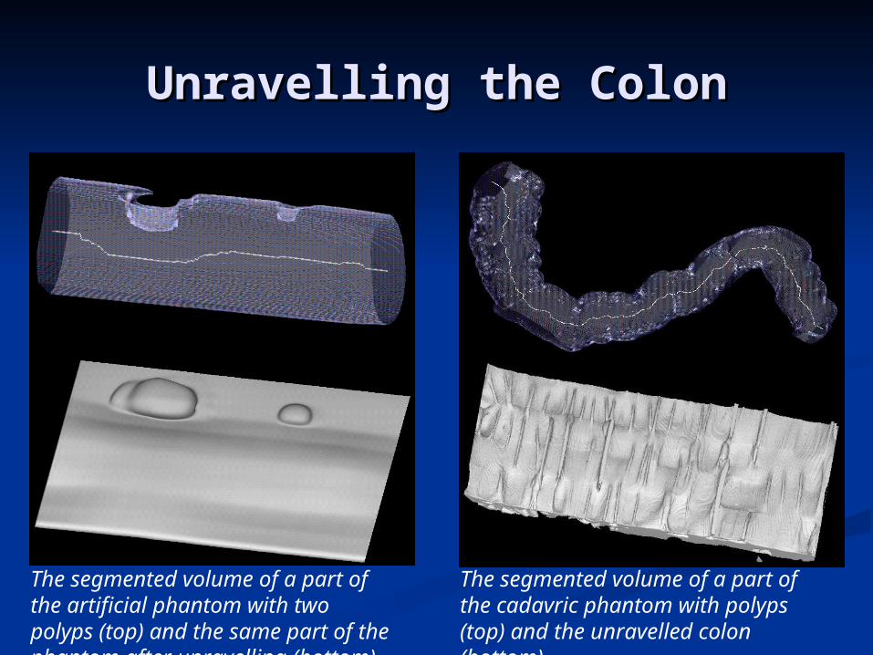
Unravelling the ColonUnravelling the Colon
Unravelling the colon is a new method to visualize Unravelling the colon is a new method to visualize the entire inner surface of the colon without the the entire inner surface of the colon without the need for navigation.need for navigation.
This is a minimally invasive technique that can be This is a minimally invasive technique that can be used for colorectal polyps and cancer detection.used for colorectal polyps and cancer detection.
An algorithm for unravelling the colon which is to An algorithm for unravelling the colon which is to digitally straighten and then flatten using digitally straighten and then flatten using reconstructed spiral/helical computer tomograph reconstructed spiral/helical computer tomograph (CT) images.(CT) images.
Comparing to virtual colonoscopy where polyps Comparing to virtual colonoscopy where polyps may be hidden from view behind the folds, the may be hidden from view behind the folds, the unravelled colon is more suitable for polyp unravelled colon is more suitable for polyp detection, because the entire inner surface is detection, because the entire inner surface is displayed at one view.displayed at one view.
Unravelling the ColonUnravelling the Colon
The segmented volume of a part of the artificial phantom with two polyps (top) and the same part of the phantom after unravelling (bottom).
The segmented volume of a part of the cadavric phantom with polyps (top) and the unravelled colon (bottom).
PATH PLANNINGPATH PLANNING
Approaches;Approaches;
RoadmapRoadmaproad map using Meadow mapsroad map using Meadow mapsroad map using visibility graphroad map using visibility graphroad map using Voronoi diagramroad map using Voronoi diagram
RRTRRT
Cell decompositionCell decompositionexact cell decompositionexact cell decompositionapproximate cell decompositionapproximate cell decompositionadaptive cell decompositionadaptive cell decomposition
Potential fieldPotential field
RoadmapRoadmap
Building a network connection between the Building a network connection between the vertices of polygonsvertices of polygons
Typically represent obstacles as polygons, Typically represent obstacles as polygons, and the camera as a pointand the camera as a point
Appropriate for polygon-based dataset , has Appropriate for polygon-based dataset , has limitation in VClimitation in VC
Path planning: road maps using Path planning: road maps using Meadow mapsMeadow maps
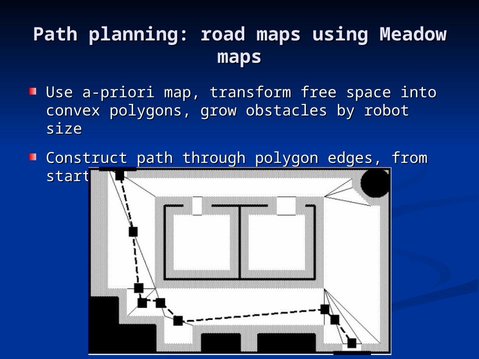
Use a-priori map, transform free space into Use a-priori map, transform free space into convex polygons, grow obstacles by robot sizeconvex polygons, grow obstacles by robot size
Construct path through polygon edges, from start Construct path through polygon edges, from start to goalto goal
Path planning: road maps using Path planning: road maps using Meadow mapsMeadow maps
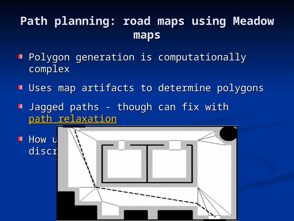
Polygon generation is computationally complexPolygon generation is computationally complex
Uses map artifacts to determine polygonsUses map artifacts to determine polygons
Jagged paths - though can fix with Jagged paths - though can fix with path relaxationpath relaxation
How update map if robot discovers discrepanciesHow update map if robot discovers discrepancies
Path planning: road map using visibility Path planning: road map using visibility graphgraph
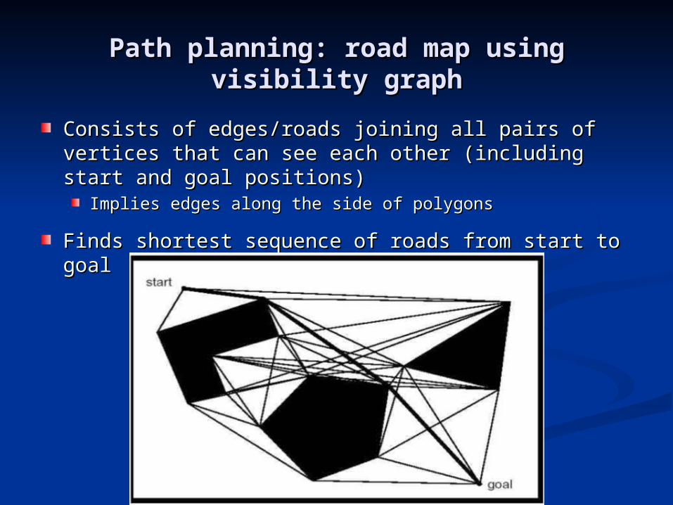
Consists of edges/roads joining all pairs of vertices Consists of edges/roads joining all pairs of vertices that can see each other (including start and goal that can see each other (including start and goal positions)positions)
Implies edges along the side of polygonsImplies edges along the side of polygons
Finds shortest sequence of roads from start to goalFinds shortest sequence of roads from start to goal
Path planning: road map using visibility Path planning: road map using visibility graphgraph
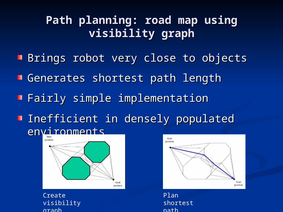
Brings robot very close to objectsBrings robot very close to objects
Generates shortest path lengthGenerates shortest path length
Fairly simple implementationFairly simple implementation
Inefficient in densely populated Inefficient in densely populated environmentsenvironments
Create visibility graph
Plan shortest path
Path planning: road map using Voronoi Path planning: road map using Voronoi diagramdiagram
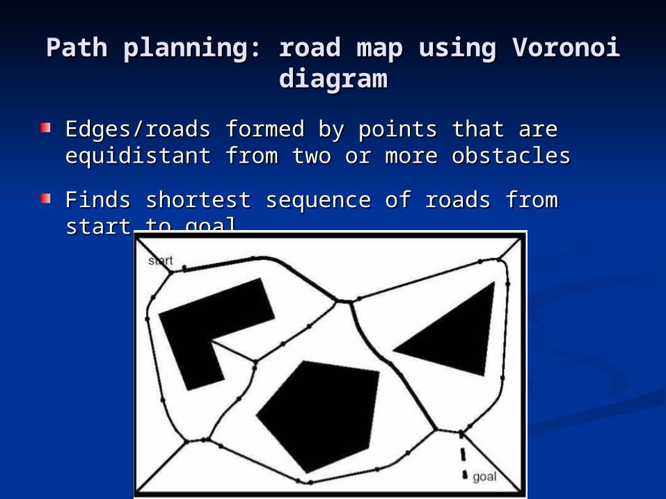
Edges/roads formed by points that are equidistant Edges/roads formed by points that are equidistant from two or more obstaclesfrom two or more obstacles
Finds shortest sequence of roads from start to Finds shortest sequence of roads from start to goalgoal
Path planning: road map using Voronoi Path planning: road map using Voronoi diagramdiagram
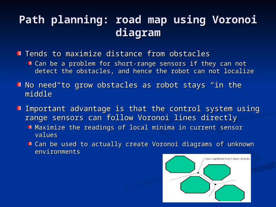
Tends to maximize distance from obstaclesTends to maximize distance from obstaclesCan be a problem for short-range sensors if they can not Can be a problem for short-range sensors if they can not detect the obstacles, and hence the robot can not localizedetect the obstacles, and hence the robot can not localize
No need to grow obstacles as robot stays “in the No need to grow obstacles as robot stays “in the middle”middle”
Important advantage is that the control system using Important advantage is that the control system using range sensors can follow Voronoi lines directlyrange sensors can follow Voronoi lines directly
Maximize the readings of local minima in current sensor valuesMaximize the readings of local minima in current sensor values
Can be used to actually create Voronoi diagrams of unknown Can be used to actually create Voronoi diagrams of unknown environmentsenvironments
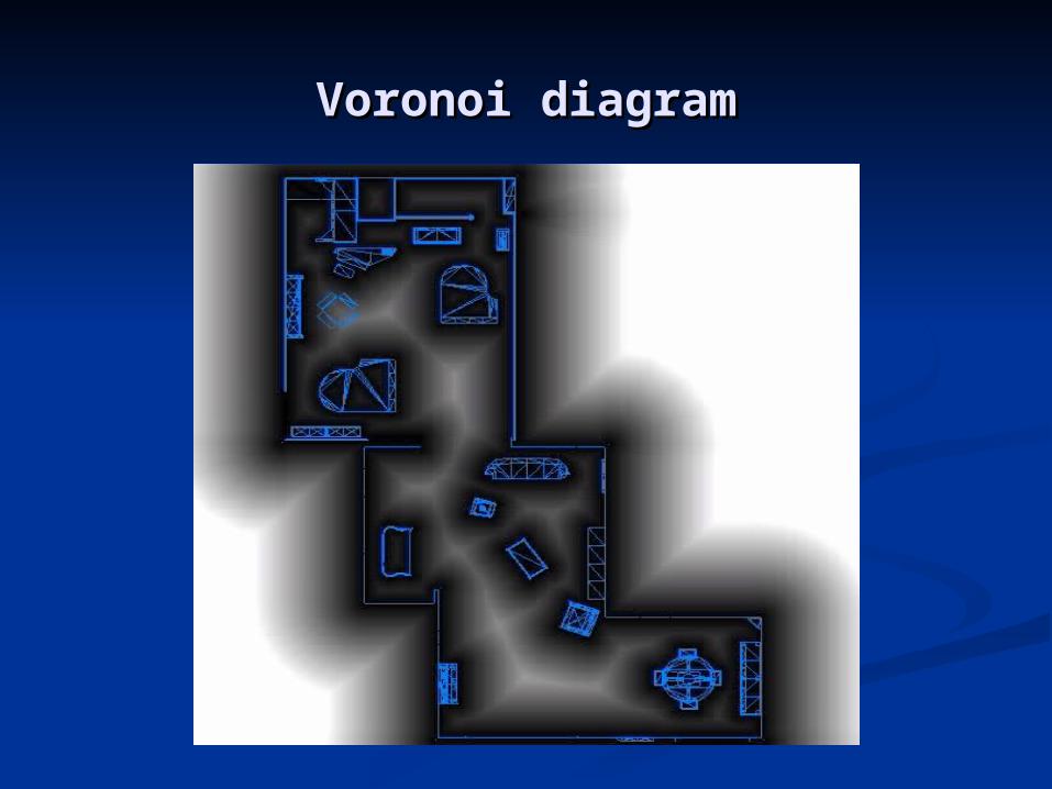
Voronoi diagramVoronoi diagram
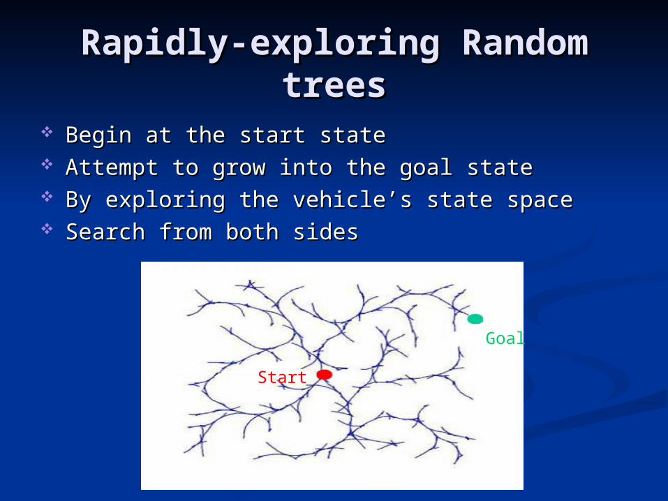
Rapidly-exploring Random Rapidly-exploring Random treestrees
Begin at the start stateBegin at the start state Attempt to grow into the goal stateAttempt to grow into the goal state By exploring the vehicle’s state spaceBy exploring the vehicle’s state space Search from both sidesSearch from both sides
Goal
Start
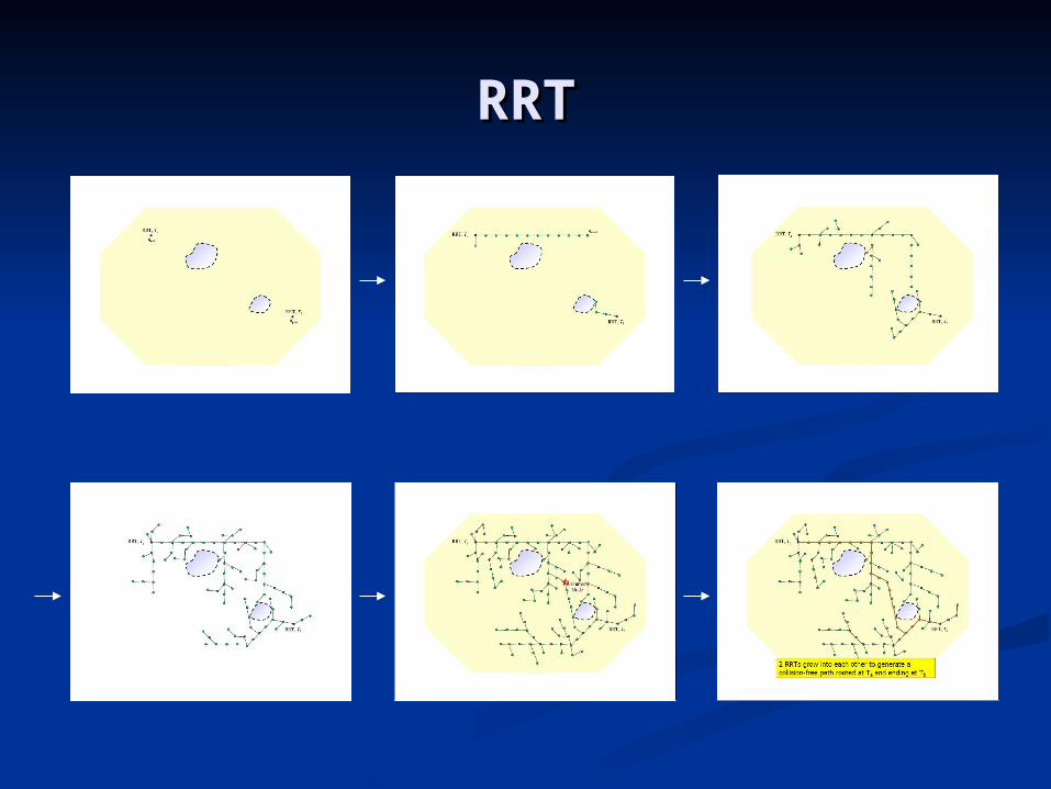
RRTRRT
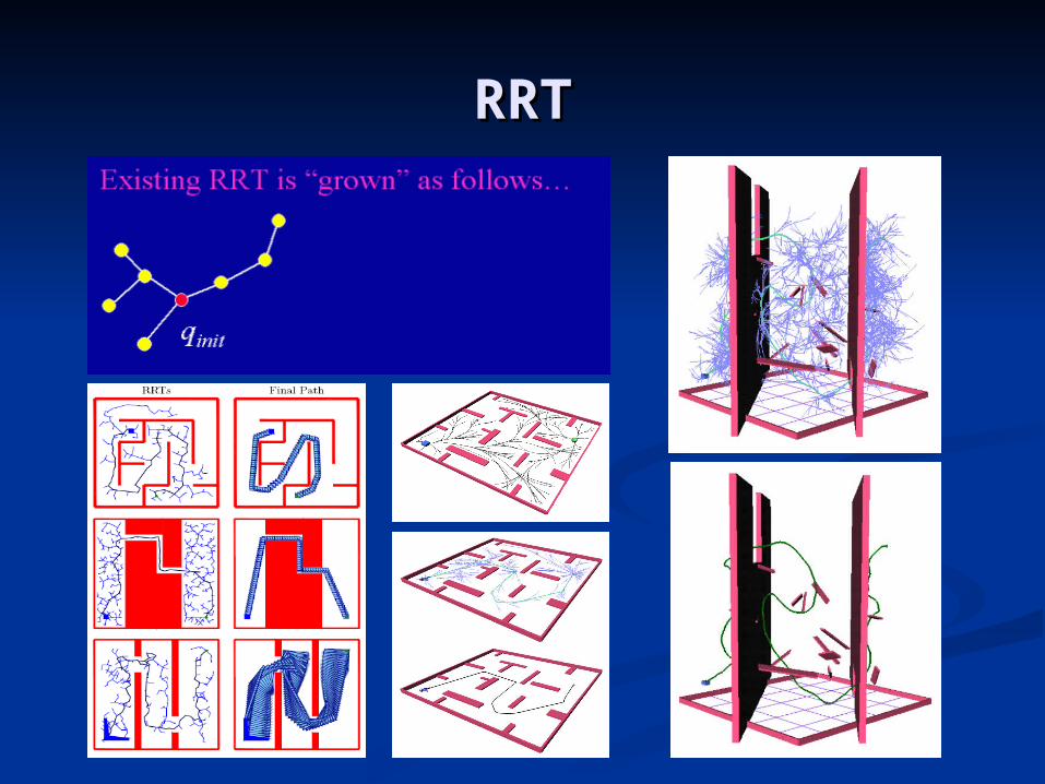
RRTRRT
Cell decompositionCell decomposition
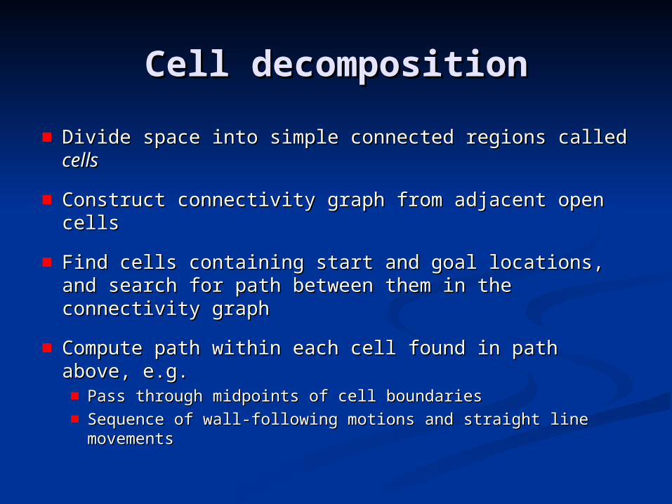
Divide space into simple connected regions called Divide space into simple connected regions called cellscells
Construct connectivity graph from adjacent open cellsConstruct connectivity graph from adjacent open cells
Find cells containing start and goal locations, and Find cells containing start and goal locations, and search for path between them in the connectivity search for path between them in the connectivity graphgraph
Compute path within each cell found in path above, Compute path within each cell found in path above, e.g.e.g.
Pass through midpoints of cell boundariesPass through midpoints of cell boundaries
Sequence of wall-following motions and straight line Sequence of wall-following motions and straight line movementsmovements
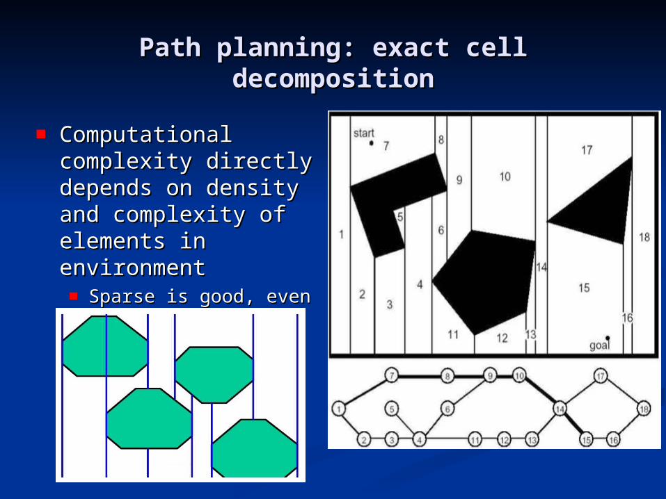
Path planning: exact cell decompositionPath planning: exact cell decomposition
Computational Computational complexity directly complexity directly depends on density depends on density and complexity of and complexity of elements in elements in environmentenvironment
Sparse is good, even for Sparse is good, even for very geometrically large very geometrically large areasareas
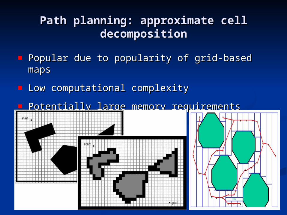
Path planning: approximate cell Path planning: approximate cell decompositiondecomposition
Popular due to popularity of grid-based mapsPopular due to popularity of grid-based maps
Low computational complexityLow computational complexity
Potentially large memory requirementsPotentially large memory requirements

Path planning: approximate cell Path planning: approximate cell decompositiondecomposition
NF1, ‘grassfire’, algorithmNF1, ‘grassfire’, algorithmMinima-freeMinima-free
Wavefront expansion from goal outwardsWavefront expansion from goal outwards
Each cell visited once - computational complexity linear Each cell visited once - computational complexity linear in number of cells, not environment complexityin number of cells, not environment complexity
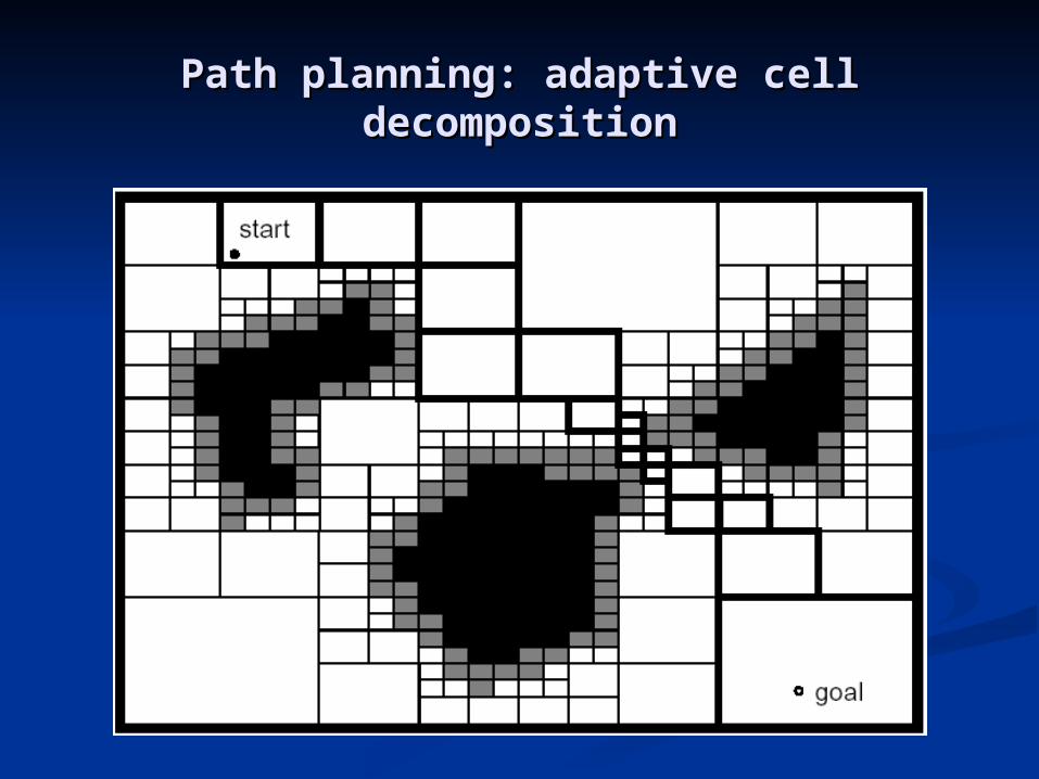
Path planning: adaptive cell Path planning: adaptive cell decompositiondecomposition
Potential fieldPotential field
This approaches is simplified to a point such as a This approaches is simplified to a point such as a camera model in computer graphicscamera model in computer graphics
The camera moves under the influence of a set of The camera moves under the influence of a set of potentials produced by the attraction and potentials produced by the attraction and repulsion potentialsrepulsion potentials
The attraction potential pulls robot toward the The attraction potential pulls robot toward the goal and the repulsion potential pushes it away goal and the repulsion potential pushes it away from the obstaclesfrom the obstacles
The variation of potentials create the attraction The variation of potentials create the attraction and repulsion forcesand repulsion forces
Path planning: potential fieldsPath planning: potential fields
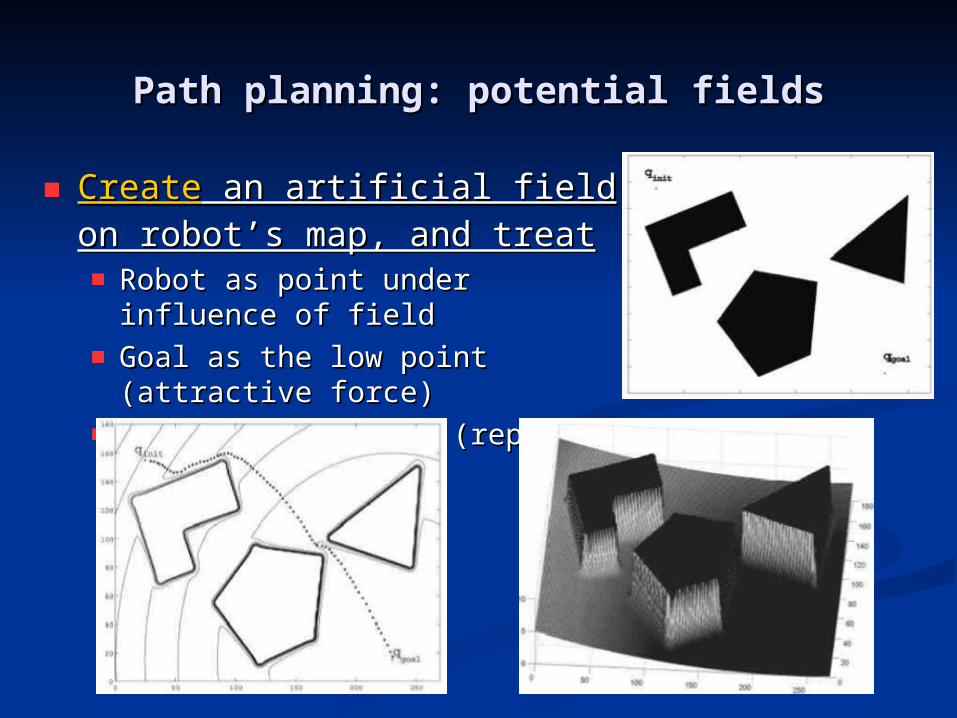
CreateCreate an artificial field on an artificial field on robot’s map, and treatrobot’s map, and treat
Robot as point under influence of Robot as point under influence of fieldfield
Goal as the low point (attractive Goal as the low point (attractive force)force)
Obstacles as peaks (repulsive Obstacles as peaks (repulsive forces)forces)
Path planning: potential fieldsPath planning: potential fields
Fairly easy to implementFairly easy to implement
Set robot speed proportional to forceSet robot speed proportional to force
Field drives robot to the goalField drives robot to the goal
Movement is similar to a ball rolling down a hillMovement is similar to a ball rolling down a hill
Is also a control law as robot can always determine Is also a control law as robot can always determine next required action (assuming robot can localize next required action (assuming robot can localize position with respect to its map and the field)position with respect to its map and the field)
Local minima can be problematicLocal minima can be problematic
Concave objects can generate oscillationsConcave objects can generate oscillations
More complicated if robot is not treated as point More complicated if robot is not treated as point massmass
Path planning: potential field, Path planning: potential field, extensionsextensions
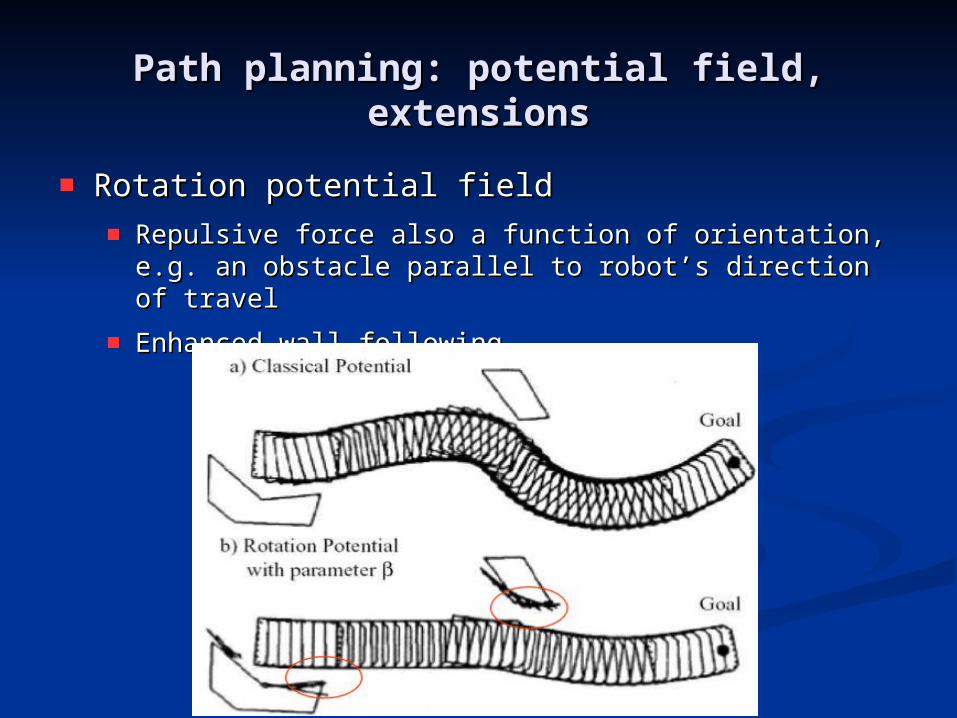
Rotation potential fieldRotation potential field
Repulsive force also a function of orientation, e.g. an Repulsive force also a function of orientation, e.g. an obstacle parallel to robot’s direction of travelobstacle parallel to robot’s direction of travel
Enhanced wall followingEnhanced wall following
Virtual Endoscopy - IdeaVirtual Endoscopy - Idea
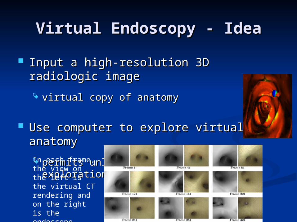
Input a high-resolution 3D radiologic Input a high-resolution 3D radiologic imageimage
virtual copy of anatomyvirtual copy of anatomy
Use computer to explore virtual anatomyUse computer to explore virtual anatomy
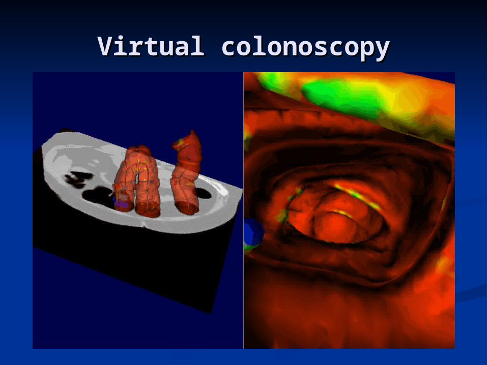
permits unlimited navigation explorationpermits unlimited navigation explorationIn each frame, the view on the left is the virtual CT rendering and on the right is the endoscope image
NavigationNavigation
The camera automatically moves from the The camera automatically moves from the source point towards the target pointsource point towards the target point
User can interactively modified the camera User can interactively modified the camera position and directionposition and direction
The camera stays away from the surfaceThe camera stays away from the surface
The camera should never penetrate through The camera should never penetrate through the surfacethe surface
The physician can change source and target The physician can change source and target positionspositions
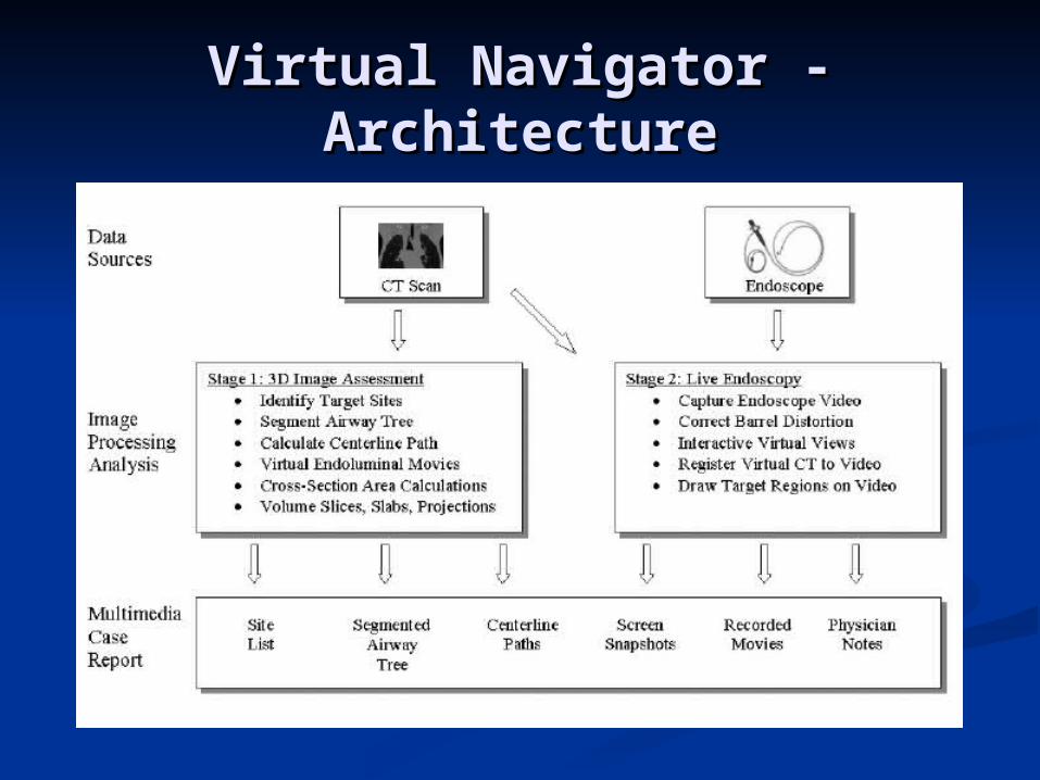
Virtual Navigator - Virtual Navigator - ArchitectureArchitecture

APPLICATIONSAPPLICATIONS
Virtual colonoscopyVirtual colonoscopy
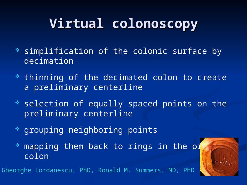
simplification of the colonic surface by decimation
thinning of the decimated colon to create a preliminary centerline
selection of equally spaced points on the preliminary centerline
grouping neighboring points
mapping them back to rings in the original colon
Gheorghe Iordanescu, PhD, Ronald M. Summers, MD, PhD
Virtual colonoscopyVirtual colonoscopy
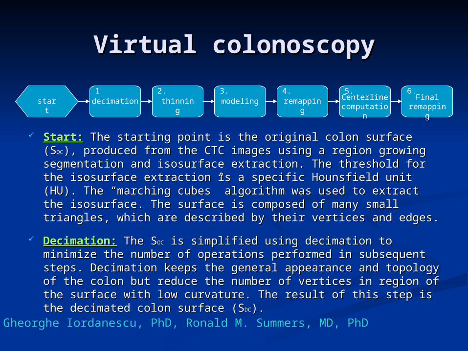
Start:Start: The starting point is the original colon surface (S The starting point is the original colon surface (SOCOC), ), produced from the CTC images using a region growing produced from the CTC images using a region growing segmentation and isosurface extraction. The threshold for the segmentation and isosurface extraction. The threshold for the isosurface extraction is a specific Hounsfield unit (HU). The isosurface extraction is a specific Hounsfield unit (HU). The “marching cubes” algorithm was used to extract the isosurface. “marching cubes” algorithm was used to extract the isosurface. The surface is composed of many small triangles, which are The surface is composed of many small triangles, which are described by their vertices and edges. described by their vertices and edges.
Decimation:Decimation: The S The SOCOC is simplified using decimation to minimize is simplified using decimation to minimize the number of operations performed in subsequent steps. the number of operations performed in subsequent steps. Decimation keeps the general appearance and topology of the Decimation keeps the general appearance and topology of the colon but reduce the number of vertices in region of the surface colon but reduce the number of vertices in region of the surface with low curvature. The result of this step is the decimated colon with low curvature. The result of this step is the decimated colon surface (Ssurface (SDCDC).).Gheorghe Iordanescu, PhD, Ronald M. Summers, MD, PhD
start decimation thinning modeling remapping
Centerline computation
Final remappin
g
1.
3.2. 4. 5. 6.
Virtual colonoscopyVirtual colonoscopy
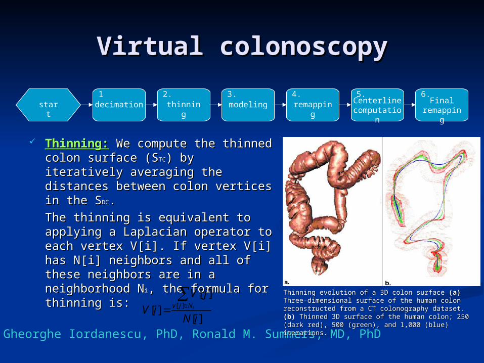
Thinning:Thinning: We compute the We compute the thinned colon surface (Sthinned colon surface (STCTC) by ) by iteratively averaging the iteratively averaging the distances between colon vertices distances between colon vertices in the Sin the SDCDC..
The thinning is equivalent to The thinning is equivalent to applying a Laplacian operator to applying a Laplacian operator to each vertex V[i]. If vertex V[i] has each vertex V[i]. If vertex V[i] has N[i] neighbors and all of these N[i] neighbors and all of these neighbors are in a neighborhood neighbors are in a neighborhood NNii, the formula for thinning is:, the formula for thinning is:
Gheorghe Iordanescu, PhD, Ronald M. Summers, MD, PhD
start decimation thinning modeling remapping
Centerline computation
Final remappin
g
1.
3.2. 4. 5. 6.
Thinning evolution of a 3D colon surface Thinning evolution of a 3D colon surface (a) (a) Three-Three-dimensional surface of the human colon reconstructed dimensional surface of the human colon reconstructed from a CT colonography dataset. from a CT colonography dataset. (b) (b) Thinned 3D surface Thinned 3D surface of the human colon; 250 (dark red), 500 (green), and of the human colon; 250 (dark red), 500 (green), and 1,000 (blue) iterations.1,000 (blue) iterations.
][
][
][ ][
iN
jV
iV iNjv
Virtual colonoscopyVirtual colonoscopy
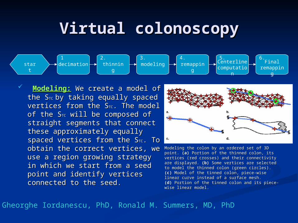
Modeling:Modeling: We create a model We create a model of the Sof the STC TC by taking equally by taking equally spaced vertices from the Sspaced vertices from the STCTC. The . The model of the Smodel of the STCTC will be composed will be composed of straight segments that of straight segments that connect these approximately connect these approximately equally spaced vertices from the equally spaced vertices from the SSTCTC. To obtain the correct . To obtain the correct vertices, we use a region growing vertices, we use a region growing strategy in which we start from a strategy in which we start from a seed point and identify vertices seed point and identify vertices connected to the seed.connected to the seed.
Gheorghe Iordanescu, PhD, Ronald M. Summers, MD, PhD
start decimation thinning modeling remapping
Centerline computation
Final remappin
g
1.
3.2. 4. 5. 6.
Modeling the colon by an ordered set of 3D point. Modeling the colon by an ordered set of 3D point. (a)(a) Portion of the thinned colon, its vertices (red crosses) Portion of the thinned colon, its vertices (red crosses) and their connectivity are displayed. and their connectivity are displayed. (b)(b) Some vertices Some vertices are selected to model the thinned colon (green circles). are selected to model the thinned colon (green circles). (c)(c) Model of the tinned colon, piece-wise linear curve Model of the tinned colon, piece-wise linear curve instead of a surface mesh. instead of a surface mesh. (d)(d) Portion of the tinned Portion of the tinned colon and its piece-wise linear model.colon and its piece-wise linear model.
Virtual colonoscopyVirtual colonoscopy
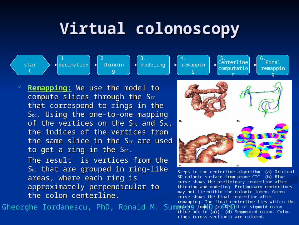
Remapping:Remapping: We use the model to We use the model to compute slices through the Scompute slices through the STCTC that that correspond to rings in the Scorrespond to rings in the SDCDC. Using . Using the one-to-one mapping of the the one-to-one mapping of the vertices on the Svertices on the STCTC and S and SDCDC, the indices , the indices of the vertices from the same slice in of the vertices from the same slice in the Sthe STCTC are used to get a ring in the are used to get a ring in the SSDCDC..
The result is vertices from the SThe result is vertices from the SDCDC that are grouped in ring-like areas, that are grouped in ring-like areas, where each ring is approximately where each ring is approximately perpendicular to the colon centerline.perpendicular to the colon centerline.
Gheorghe Iordanescu, PhD, Ronald M. Summers, MD, PhD
start decimation thinning modeling remapping
Centerline computation
Final remappin
g
1.
3.2. 4. 5. 6.
Steps in the centerline algorithm. (a) Original 3D colonic surface from prone CTC. (b) Blue curve shows the preliminary centerline after thinning and modeling. Preliminary centerlines may not lie within the colonic lumen. Green curve shows the final centerline after remapping. The final centerline lies within the colonic lumen. (c) Detail of sigmoid colon (blue box in (a)). (d) Segmented colon. Colon rings (cross-sections) are colored.
Virtual colonoscopyVirtual colonoscopy
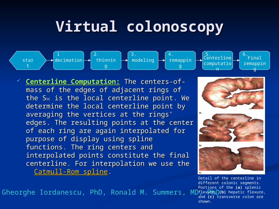
Centerline Computation:Centerline Computation: The centers- The centers-of-mass of the edges of adjacent rings of of-mass of the edges of adjacent rings of the Sthe SDCDC is the local centerline point. We is the local centerline point. We determine the local centerline point by determine the local centerline point by averaging the vertices at the rings’ edges. averaging the vertices at the rings’ edges. The resulting points at the center of each The resulting points at the center of each ring are again interpolated for purpose of ring are again interpolated for purpose of display using spline functions. The ring display using spline functions. The ring centers and interpolated points constitute centers and interpolated points constitute the final centerline. For interpolation we the final centerline. For interpolation we use the use the CatmullCatmull-Rom spline-Rom spline..
Gheorghe Iordanescu, PhD, Ronald M. Summers, MD, PhD
start decimation thinning modeling remapping
Centerline computation
Final remappin
g
1.
3.2. 4. 5. 6.
Detail of the centerline in different colonic segments. Portions of the (a) splenic flexure, (b) hepatic flexure, and (c) transverse colon are shown.
Virtual colonoscopyVirtual colonoscopy
Mapping the SMapping the SDCDC to the S to the SOCOC:: A second mapper associates A second mapper associates vertices in the Svertices in the SDCDC with the vertices in the S with the vertices in the SOCOC based on based on minimum distance criterion between the vertices of the two minimum distance criterion between the vertices of the two surfaces. Based on the correspondence of the vertices on the surfaces. Based on the correspondence of the vertices on the SSDCDC and S and SOCOC we can segment the S we can segment the SOCOC and split the surface into and split the surface into rings. rings.
To limit the search space and improve computational To limit the search space and improve computational efficiency in performing this second mapping , a process called efficiency in performing this second mapping , a process called “vertex classification” is performed, vertices in the S“vertex classification” is performed, vertices in the SDCDC and S and SOCOC are grouped into classes according to their spatial coordinates. are grouped into classes according to their spatial coordinates. Because only vertices in neighboring classes need to be Because only vertices in neighboring classes need to be searched, there is a substantial performance improvement.searched, there is a substantial performance improvement.
Gheorghe Iordanescu, PhD, Ronald M. Summers, MD, PhD
start decimation thinning modeling remapping
Centerline computation
Final remappin
g
1.
3.2. 4. 5. 6.
Virtual colonoscopyVirtual colonoscopy
Virtual Endoscopy Virtual Endoscopy (based on potential (based on potential fields)fields)
The idea is to utilize a hierarchical analysis of The idea is to utilize a hierarchical analysis of attractors to determine principal attractorsattractors to determine principal attractors
We combine potentials derived from the distance We combine potentials derived from the distance between source and target positions and from the between source and target positions and from the distance to the colon surface to guide path search distance to the colon surface to guide path search process, the paths far away from the colon wall and in process, the paths far away from the colon wall and in the direction of target positionthe direction of target position
Advantages:Advantages: Eliminating small-undesired branches during the attractor Eliminating small-undesired branches during the attractor
analysis.analysis. Warranty of connectivity between start and target points.Warranty of connectivity between start and target points. Search of paths just between principal attractors and do not Search of paths just between principal attractors and do not
waste time in connecting the small attractors.waste time in connecting the small attractors.Rui C. H. Chiou, Arie E. Kaufman, Zhengrong Liang, Lichan Hong and Miranda Achniotou
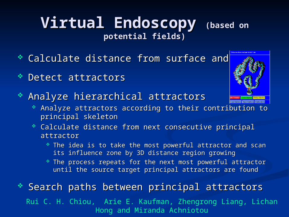
Virtual Endoscopy Virtual Endoscopy (based on potential (based on potential fields)fields)
Calculate distance from surface and targetCalculate distance from surface and target
Detect attractorsDetect attractors
Analyze hierarchical attractorsAnalyze hierarchical attractors Analyze attractors according to their contribution to principal Analyze attractors according to their contribution to principal
skeletonskeleton Calculate distance from next consecutive principal attractorCalculate distance from next consecutive principal attractor
The idea is to take the most powerful attractor and scan its The idea is to take the most powerful attractor and scan its influence zone by 3D distance region growinginfluence zone by 3D distance region growing
The process repeats for the next most powerful attractor until the The process repeats for the next most powerful attractor until the source target principal attractors are foundsource target principal attractors are found
Search paths between principal attractorsSearch paths between principal attractors
Rui C. H. Chiou, Arie E. Kaufman, Zhengrong Liang, Lichan Hong and Miranda Achniotou
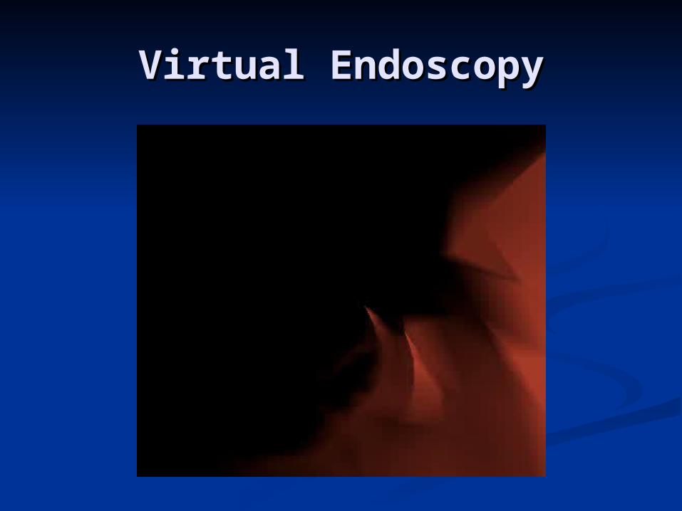
Virtual EndoscopyVirtual Endoscopy
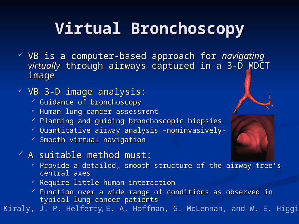
Virtual BronchoscopyVirtual Bronchoscopy
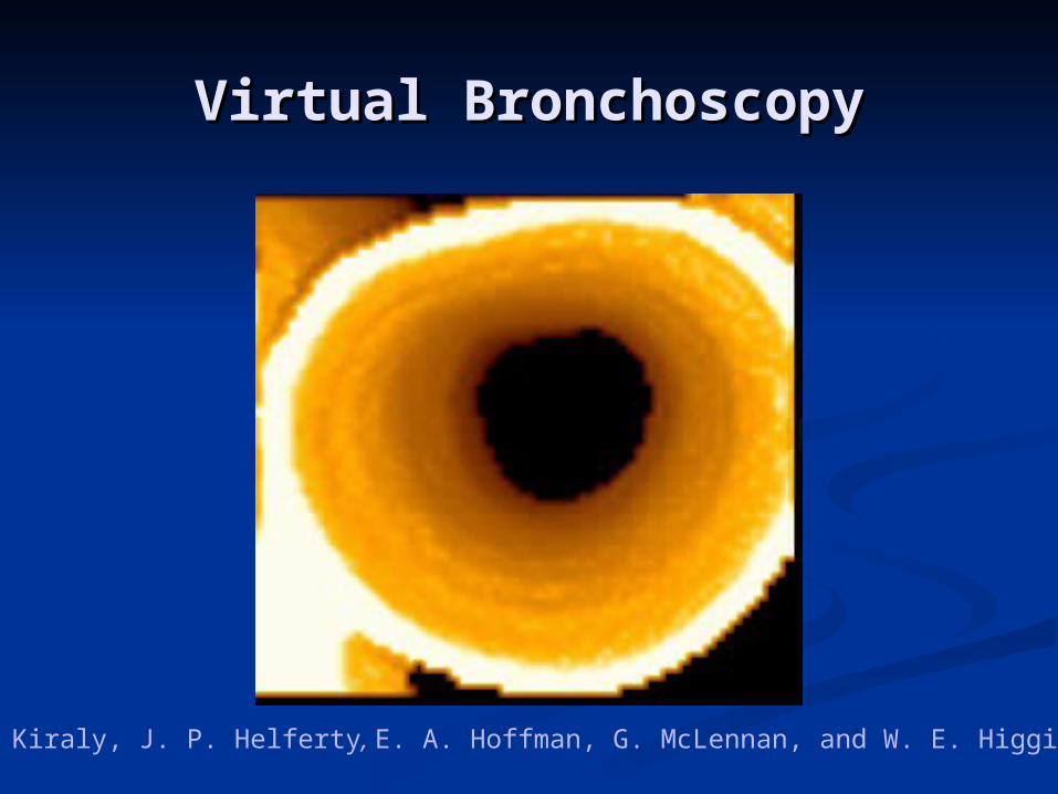
VB is a computer-based approach for VB is a computer-based approach for navigating navigating virtuallyvirtually through airways captured in a 3-D MDCT through airways captured in a 3-D MDCT imageimage
VB 3-D image analysis:VB 3-D image analysis: Guidance of bronchoscopyGuidance of bronchoscopy Human lung-cancer assessment Human lung-cancer assessment Planning and guiding bronchoscopic biopsiesPlanning and guiding bronchoscopic biopsies Quantitative airway analysis –noninvasively-Quantitative airway analysis –noninvasively- Smooth virtual navigationSmooth virtual navigation
A suitable method must:A suitable method must: Provide a detailed, smooth structure of the airway tree’s central Provide a detailed, smooth structure of the airway tree’s central
axesaxes Require little human interactionRequire little human interaction Function over a wide range of conditions as observed in typical Function over a wide range of conditions as observed in typical
lung-cancer patientslung-cancer patientsA. P. Kiraly, J. P. Helferty, E. A. Hoffman, G. McLennan, and W. E. Higgins
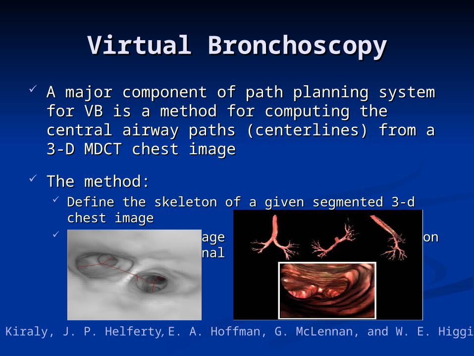
Virtual BronchoscopyVirtual Bronchoscopy
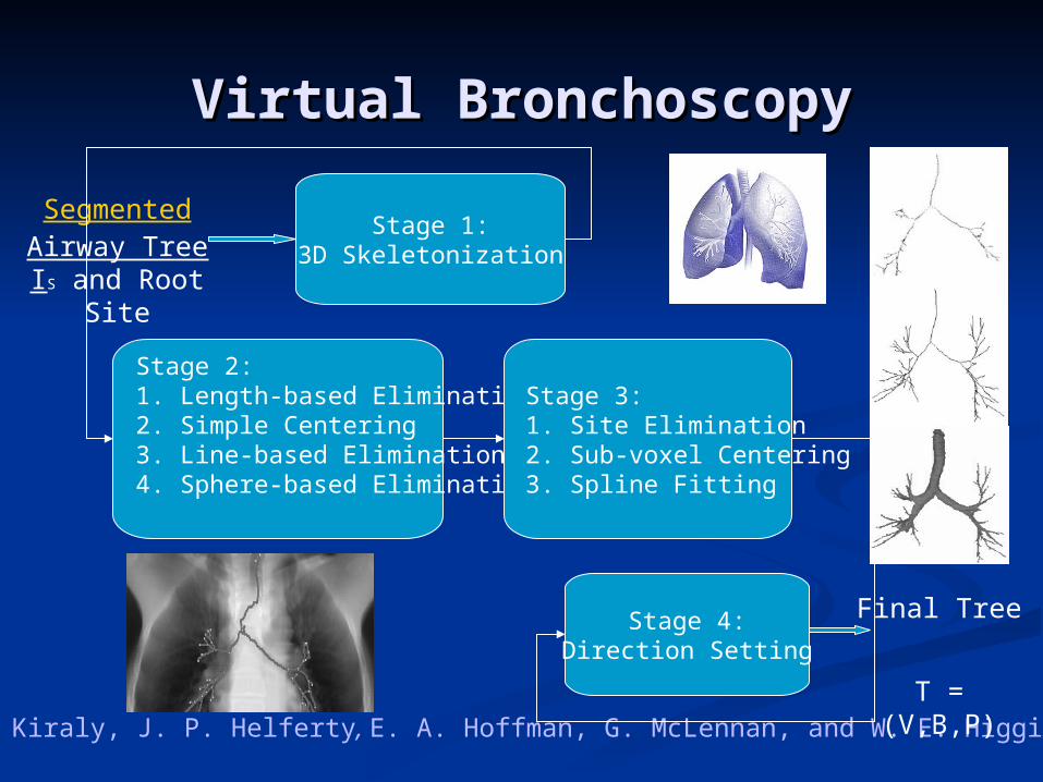
A major component of path planning system for A major component of path planning system for VB is a method for computing the central airway VB is a method for computing the central airway paths (centerlines) from a 3-D MDCT chest imagepaths (centerlines) from a 3-D MDCT chest image
The method:The method: Define the skeleton of a given segmented 3-d chest Define the skeleton of a given segmented 3-d chest
imageimage Perform a multistage refinement of the skeleton to Perform a multistage refinement of the skeleton to
arrive at a final tree structurearrive at a final tree structure
A. P. Kiraly, J. P. Helferty, E. A. Hoffman, G. McLennan, and W. E. Higgins
Virtual BronchoscopyVirtual Bronchoscopy
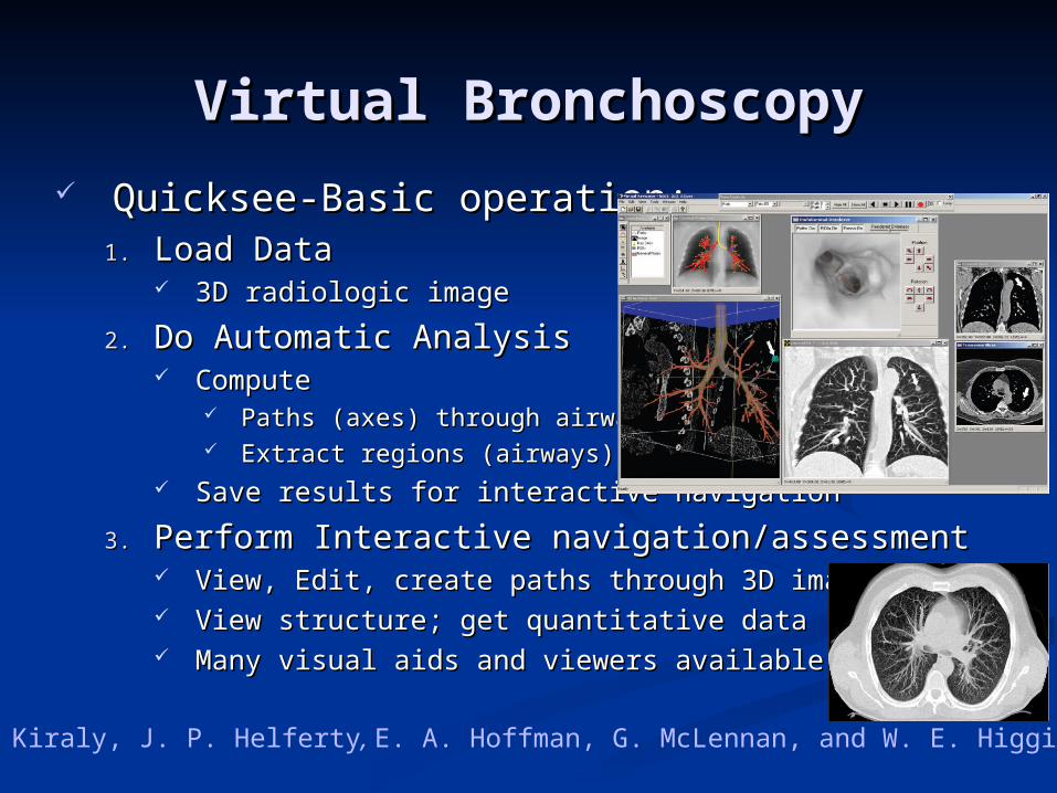
Quicksee-Basic operation:Quicksee-Basic operation:1.1. Load DataLoad Data
3D radiologic image3D radiologic image
2.2. Do Automatic AnalysisDo Automatic Analysis ComputeCompute
Paths (axes) through airwaysPaths (axes) through airways Extract regions (airways)Extract regions (airways)
Save results for interactive navigationSave results for interactive navigation
3.3. Perform Interactive navigation/assessmentPerform Interactive navigation/assessment View, Edit, create paths through 3D imageView, Edit, create paths through 3D image View structure; get quantitative dataView structure; get quantitative data Many visual aids and viewers availableMany visual aids and viewers available
A. P. Kiraly, J. P. Helferty, E. A. Hoffman, G. McLennan, and W. E. Higgins
Virtual BronchoscopyVirtual Bronchoscopy
A. P. Kiraly, J. P. Helferty, E. A. Hoffman, G. McLennan, and W. E. Higgins
Segmented Airway Tree IS and Root Site
Stage 1:3D Skeletonization
Stage 2:1. Length-based Elimination2. Simple Centering3. Line-based Elimination4. Sphere-based Elimination
Stage 3:1. Site Elimination2. Sub-voxel Centering3. Spline Fitting
Stage 4:Direction Setting
Final Tree
T = (V,B,P)
Virtual BronchoscopyVirtual Bronchoscopy
A. P. Kiraly, J. P. Helferty, E. A. Hoffman, G. McLennan, and W. E. Higgins
OUR WORKOUR WORK
Goals:Goals: The aim of our work is to build trajectories for virtual The aim of our work is to build trajectories for virtual
endoscopy inside 3D medical images, using the endoscopy inside 3D medical images, using the most most automatic wayautomatic way..
Virtual endoscopy results are shown in various anatomical Virtual endoscopy results are shown in various anatomical regions (bronchi, colon, brain vessels, arteries) with regions (bronchi, colon, brain vessels, arteries) with different 3D imaging protocols (CT, MR).different 3D imaging protocols (CT, MR).
In my thesis, an automatic centerline determination In my thesis, an automatic centerline determination algorithm for three dimensional virtual bronchoscopy CT algorithm for three dimensional virtual bronchoscopy CT image will be present.image will be present.
We try that our method:We try that our method: Be fasterBe faster
Needs less interactionNeeds less interaction
Be more robust and reproducibleBe more robust and reproducible
OUR WORKOUR WORK
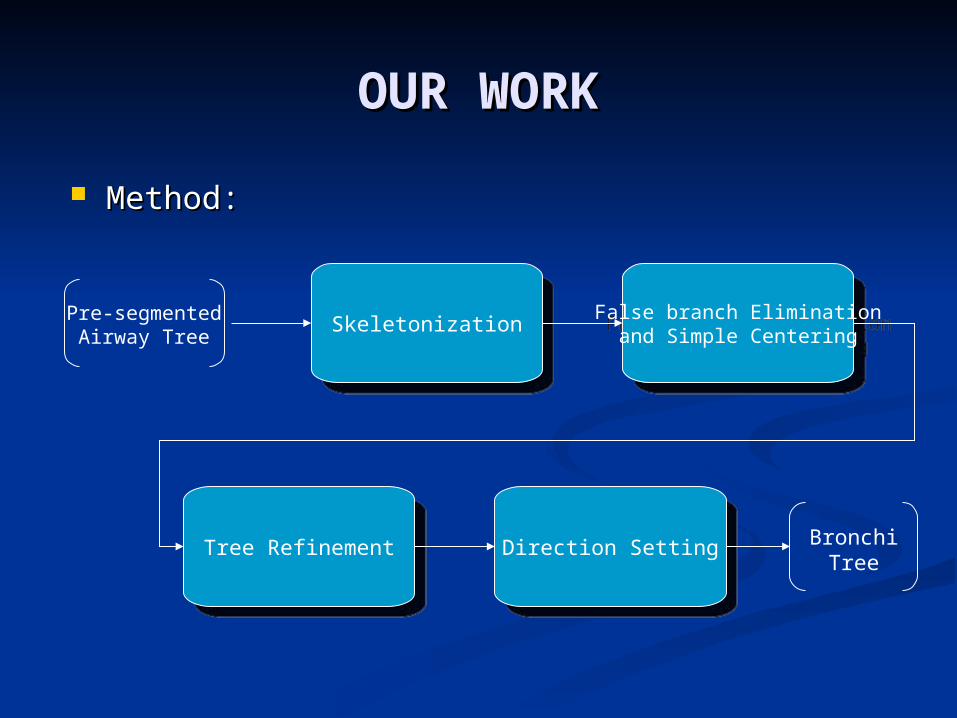
Method:Method:
SkeletonizationSkeletonization False branch Eliminationand Simple Centering
False branch Eliminationand Simple Centering
Tree RefinementTree Refinement Direction SettingDirection Setting
Pre-segmentedAirway Tree
Bronchi Tree
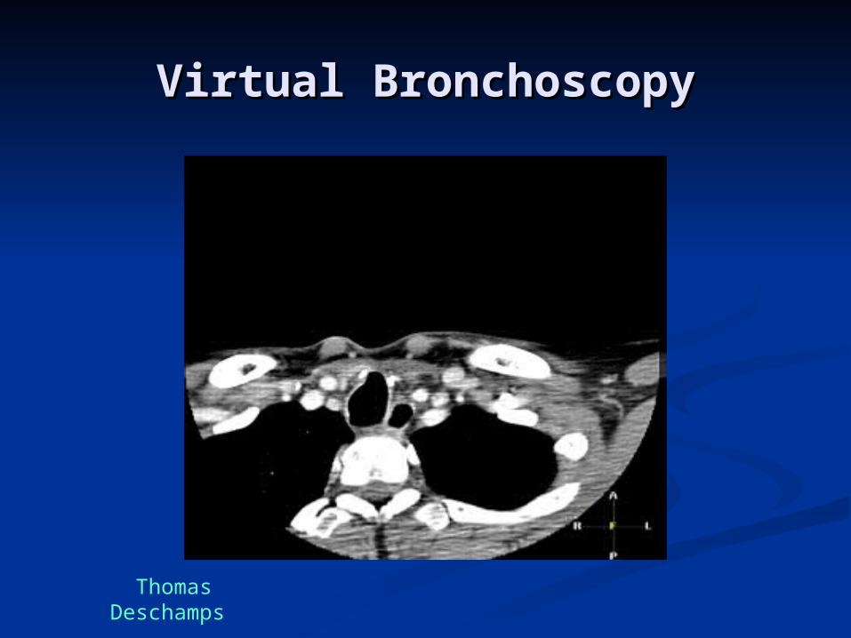
Virtual BronchoscopyVirtual Bronchoscopy
Thomas Deschamps
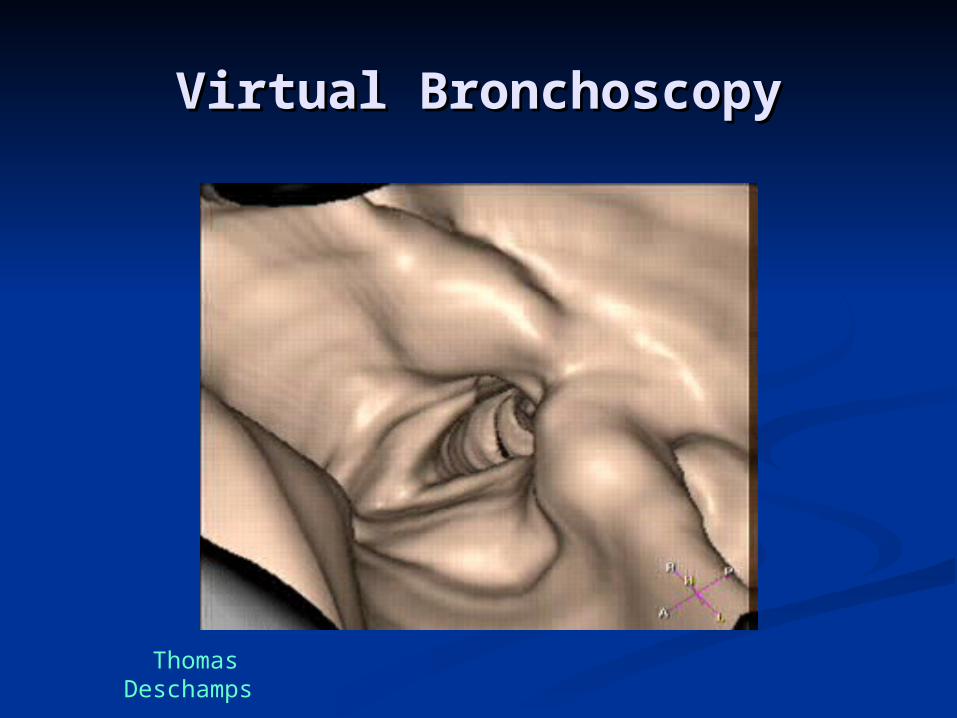
Virtual BronchoscopyVirtual Bronchoscopy
Thomas Deschamps
DiscussionDiscussion
Questions …. Suggestions …. Comments …. Ideas …. ?Questions …. Suggestions …. Comments …. Ideas …. ?
[email protected] [email protected] [email protected] [email protected]