Path Loss - Laboratório de Comunicações e Sinaisablima/grad/tfm/slides/Torlak/...EE4367 Telecom. Switching & Transmission Prof. Murat Torlak Linear Path Loss Suppose s(t) of power

EE4367 Telecom. Switching & Transmission Prof. Murat Torlak

Path LossPath Loss


Radio Wave PropagationRadio Wave Propagation

� The wireless radio channel puts fundamental limitations to

the performance of wireless communications systems

� Radio channels are extremely random, and are not easily

analyzed

� Modeling the radio channel is typically done in statistical

fashion


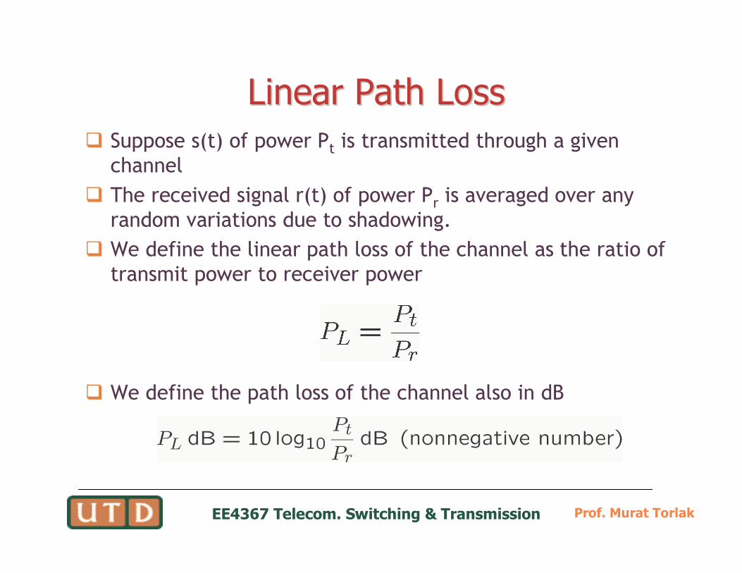
Linear Path LossLinear Path Loss

� Suppose s(t) of power Pt is transmitted through a given

channel

� The received signal r(t) of power Pr is averaged over any

random variations due to shadowing.

� We define the linear path loss of the channel as the ratio of

transmit power to receiver power

� We define the path loss of the channel also in dB


Experimental resultsExperimental results� The measurements and predictions for the receiving van driven

along 19th St./Nash St.

Prediction with distanceAnd transmission frequency


LineLine--ofof--Sight PropagationSight Propagation

� Attenuation

� The strength of a signal falls off with distance

� Free Space Propagation

� The transmitter and receiver have a clear line of sight path

between them. No other sources of impairment!

� Satellite systems and microwave systems undergo free space

propagation

� The free space power received by an antenna which is

separated from a radiating antenna by a distance is given by

Friis free space equation


FriisFriis Free Space EquationFree Space Equation� The relation between the transmit and receive power is given by

Friis free space equations:

� Gt and Gr are the transmit and receive antenna gains

� λ is the wavelength

� d is the T-R separation

� Pt is the transmitted power

� Pr is the received power

� Pt and Pr are in same units

� Gt and Gr are dimensionless quantities.

2

2(4 )r t t rP PG Gd

λπ

=

d GrGt

Pt Pr


Free Space Propagation ExampleFree Space Propagation Example

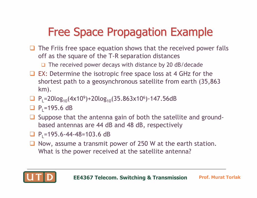
� The Friis free space equation shows that the received power falls

off as the square of the T-R separation distances

� The received power decays with distance by 20 dB/decade

� EX: Determine the isotropic free space loss at 4 GHz for the

shortest path to a geosynchronous satellite from earth (35,863

km).

� PL=20log10(4x109)+20log10(35.863x10

6)-147.56dB

� PL=195.6 dB

� Suppose that the antenna gain of both the satellite and ground-

based antennas are 44 dB and 48 dB, respectively

� PL=195.6-44-48=103.6 dB

� Now, assume a transmit power of 250 W at the earth station.

What is the power received at the satellite antenna?


Basic Propagation MechanismsBasic Propagation Mechanisms

� Reflection, diffraction, and scattering:

� Reflection occurs when a propagating electromagnetic

wave impinges upon an object

� Diffraction occurs when the radio path between the

transmitter and receiver is obstructed by a surface that has

sharp edges

� Scattering occurs when the medium through which the

wave travels

� consists of objects with dimensions that are small compared

to the wavelength, or

� the number of obstacles per unit volume is large.


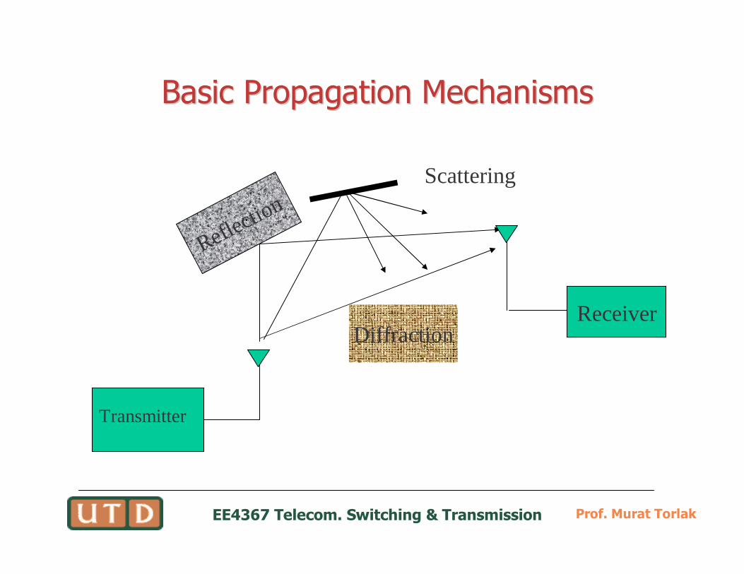
Basic Propagation MechanismsBasic Propagation Mechanisms

Reflection

Transmitter

ReceiverDiffraction

Scattering


Free Space PropagationFree Space Propagation

� Can be also expressed in relation to a reference point, d0

� K is a unitless constant that depends on the antenna

characteristics and free-space path loss up to distance d0

� Typical value for d0:

� Indoor:1m

� Outdoor: 100m to 1 km

2

00( ) d dr t

dP d PK

d = ≥

do

d

P

Reference point


Simplified Path Loss ModelSimplified Path Loss Model

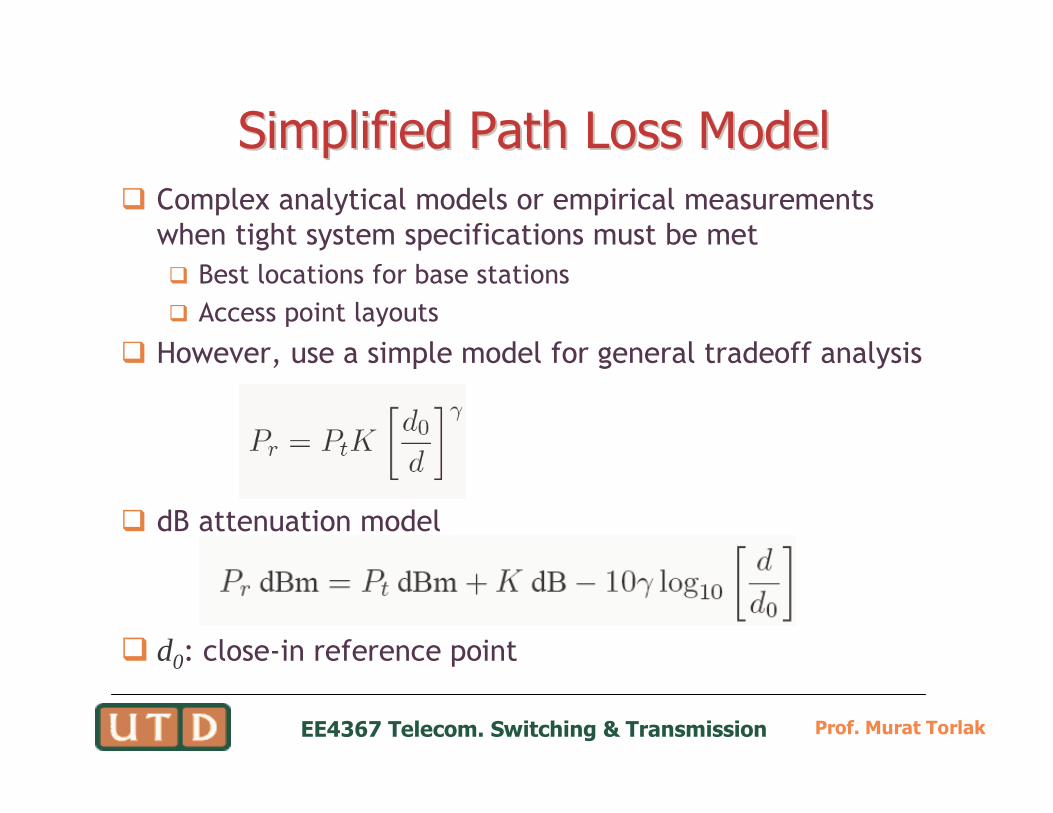
� Complex analytical models or empirical measurements

when tight system specifications must be met

� Best locations for base stations

� Access point layouts

� However, use a simple model for general tradeoff analysis

� dB attenuation model

� d0: close-in reference point


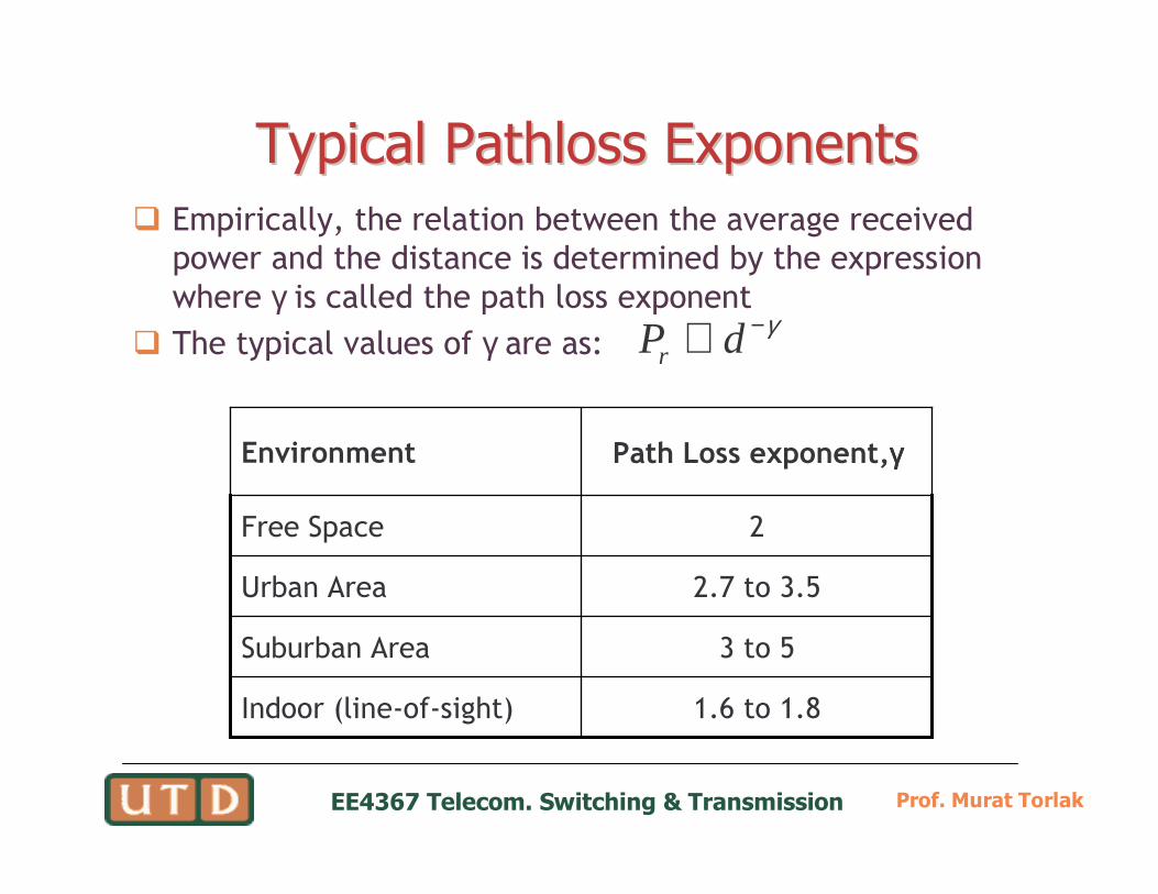
Typical Typical PathlossPathloss ExponentsExponents

� Empirically, the relation between the average received

power and the distance is determined by the expression

where γ is called the path loss exponent

� The typical values of γ are as: rP d γ−∝

1.6 to 1.8Indoor (line-of-sight)

3 to 5Suburban Area

2.7 to 3.5Urban Area

2Free Space

Path Loss exponent,γγγγEnvironment


Cell Radius PredictionCell Radius Prediction

� The signal level is same on a circle centered at the base

station with radius R

� Find the distance R such that the received signal power

cannot be less than Pmin dBm

� The received signal power at a distance d=R is specified by

� Solving the above equation for the radius R, we obtain

� where PT=Pmin-Pt-10log10K


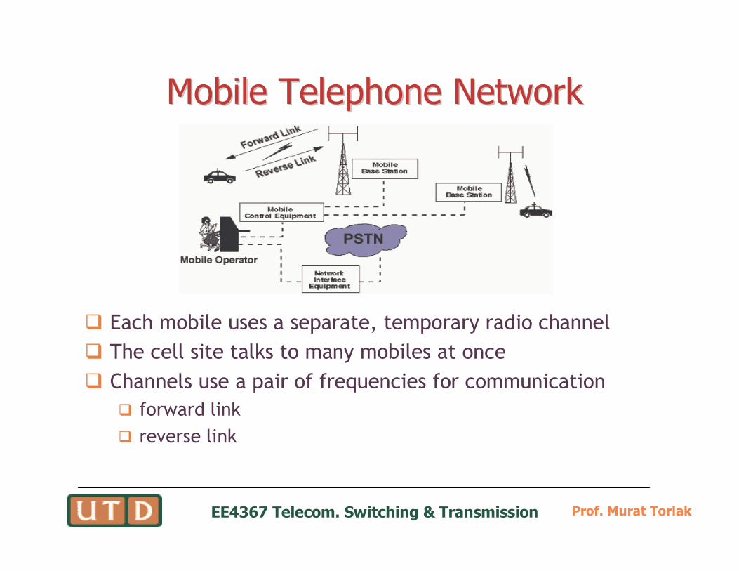
Mobile Telephone NetworkMobile Telephone Network

� Each mobile uses a separate, temporary radio channel

� The cell site talks to many mobiles at once

� Channels use a pair of frequencies for communication

� forward link

� reverse link


Limited Resource Limited Resource �� SpectrumSpectrum

� Wireline communications, i.e., optical, 10-10

� Wireless communications impairments far more severe

� 10-2 and 10-3 are typical operating BER for wireless links

� More bandwidth can improve the BER and complex modulation

and coding schemes

� Everybody wants bandwidth in wireless, more users

� How to share the spectrum for accommodating more users


Early Mobile Telephone SystemEarly Mobile Telephone System

� Traditional mobile service was structured in a fashion similar to television broadcasting

� One very powerful transmitter located at the highest spot in an area would broadcast in a radius of up to 50 kilometers

� This approach achieved very good coverage, but it was impossibleto reuse the frequencies throughout the system because of interference


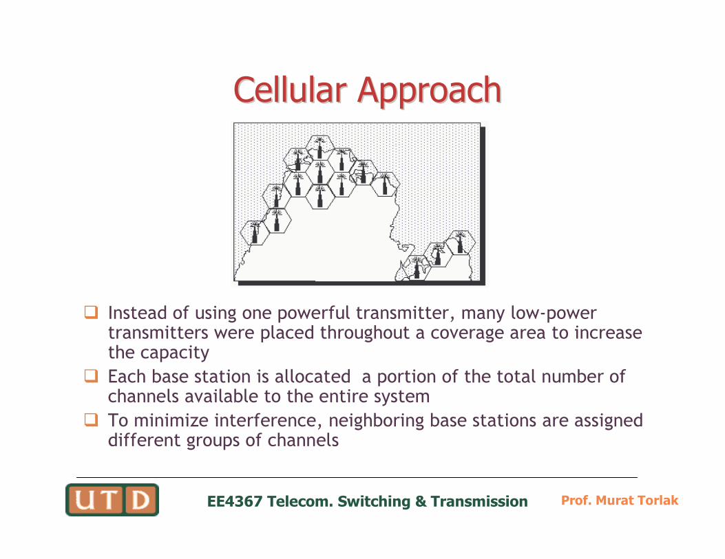
Cellular ApproachCellular Approach

� Instead of using one powerful transmitter, many low-power transmitters were placed throughout a coverage area to increase the capacity

� Each base station is allocated a portion of the total number ofchannels available to the entire system

� To minimize interference, neighboring base stations are assigneddifferent groups of channels


Why Cellular?Why Cellular?

� By systematically spacing base stations and their channel

groups, the available channels are:

� distributed throughout the geographic region

� maybe reused as many times as necessary provided that the

interference level is acceptable

� As the demand for service increases the number of base

stations may be increased thereby providing additional

radio capacity

� This enables a fixed number of channels to serve an

arbitrarily large number of subscribers by reusing the

channel throughout the coverage region


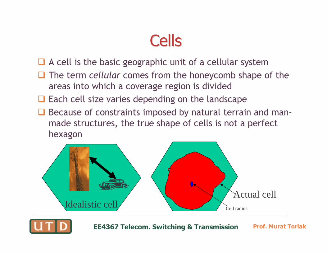
CellsCells

� A cell is the basic geographic unit of a cellular system

� The term cellular comes from the honeycomb shape of the

areas into which a coverage region is divided

� Each cell size varies depending on the landscape

� Because of constraints imposed by natural terrain and man-

made structures, the true shape of cells is not a perfect

hexagon

Idealistic cell Cell radius

Actual cell


Cell Cluster ConceptCell Cluster Concept

� A cluster is a group of cells

� No channels are reused within a cluster


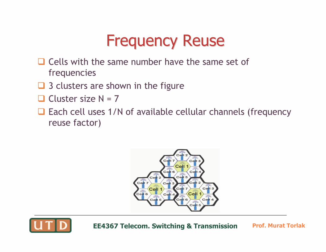
Frequency ReuseFrequency Reuse

� Cells with the same number have the same set of

frequencies

� 3 clusters are shown in the figure

� Cluster size N = 7

� Each cell uses 1/N of available cellular channels (frequency

reuse factor)


Method for finding CoMethod for finding Co--channel Cellschannel Cells� Hexagonal cells: N can only have values which satisfy N = i2 + ij +

j2 where i and j are non-negative integers

� To find the nearest co-channel neighbors of a particular cell one

must do the following

� Move i cells along any chain of hexagons

� Turn 60 degrees counter-clockwise and move j cells

� This method is illustrated for i = 2 and j = 1


Hexagonal Cell ClustersHexagonal Cell Clusters

1

89

10112

3

45

6

712

1314

1516

17

18

19

819

1

89

10112

3

45

6

712

1314

1516

17

18

19

1

89

2

56

7

1617

18

19

1

910

1123

45

6

712

1314

1516

17

181

910

1123

45

12

1314

1

2

3

1

2

3

5

8

11

8

1

2

3

8

11

5

7 7

6

10

9

12

46

7

9

4

5

6

7

9

10

6 4

1

2

3

4

5

6

7

1

2

3

4

5

6

7 1

2

3

4

5

6

7

1

2

3

4

5

6

7

4

3 6

5

2

1

2

3

4

4

2 1

3

1

3

4

2

1

3

4

2

4

3

1

3

(a) i 5 2 and j 5 0 (b) i 5 1 and j 5 2

(c) i 5 2 and j 5 2 (d) i 5 2 and j 5 3


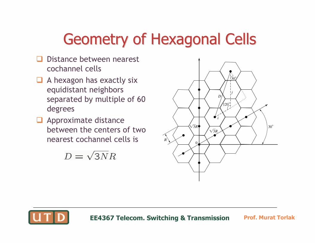
Geometry of Hexagonal CellsGeometry of Hexagonal Cells� Distance between nearest

cochannel cells

� A hexagon has exactly six

equidistant neighbors

separated by multiple of 60

degrees

� Approximate distance

between the centers of two

nearest cochannel cells is R

Ï3R

Ï3R

0

30

120

j

i

D

30


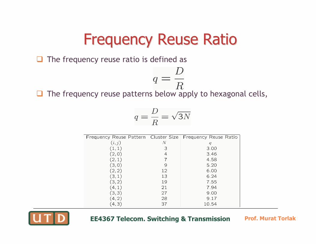
Frequency Reuse RatioFrequency Reuse Ratio� The frequency reuse ratio is defined as

� The frequency reuse patterns below apply to hexagonal cells,


CoCo--channel Interference and System Capacitychannel Interference and System Capacity

� There are several cells that use the same set of frequencies

in a given coverage area

� these cells are called co-channel cells

� the interference between signals from these cells is co-

channel interference

� Co-channel interference cannot be combated by simply

increasing the carrier power of a transmitter

� an increase in carrier transmit power increases the

interference to neighboring co-channel cells

� To reduce co-channel interference

� co-channel cells must be physically separated by a minimum

distance to provide sufficient isolation due to propagation


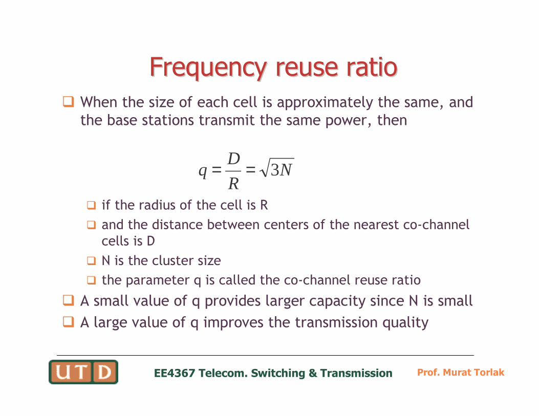
Frequency reuse ratioFrequency reuse ratio

� When the size of each cell is approximately the same, and

the base stations transmit the same power, then

� if the radius of the cell is R

� and the distance between centers of the nearest co-channel

cells is D

� N is the cluster size

� the parameter q is called the co-channel reuse ratio

� A small value of q provides larger capacity since N is small

� A large value of q improves the transmission quality

NR

Dq 3==


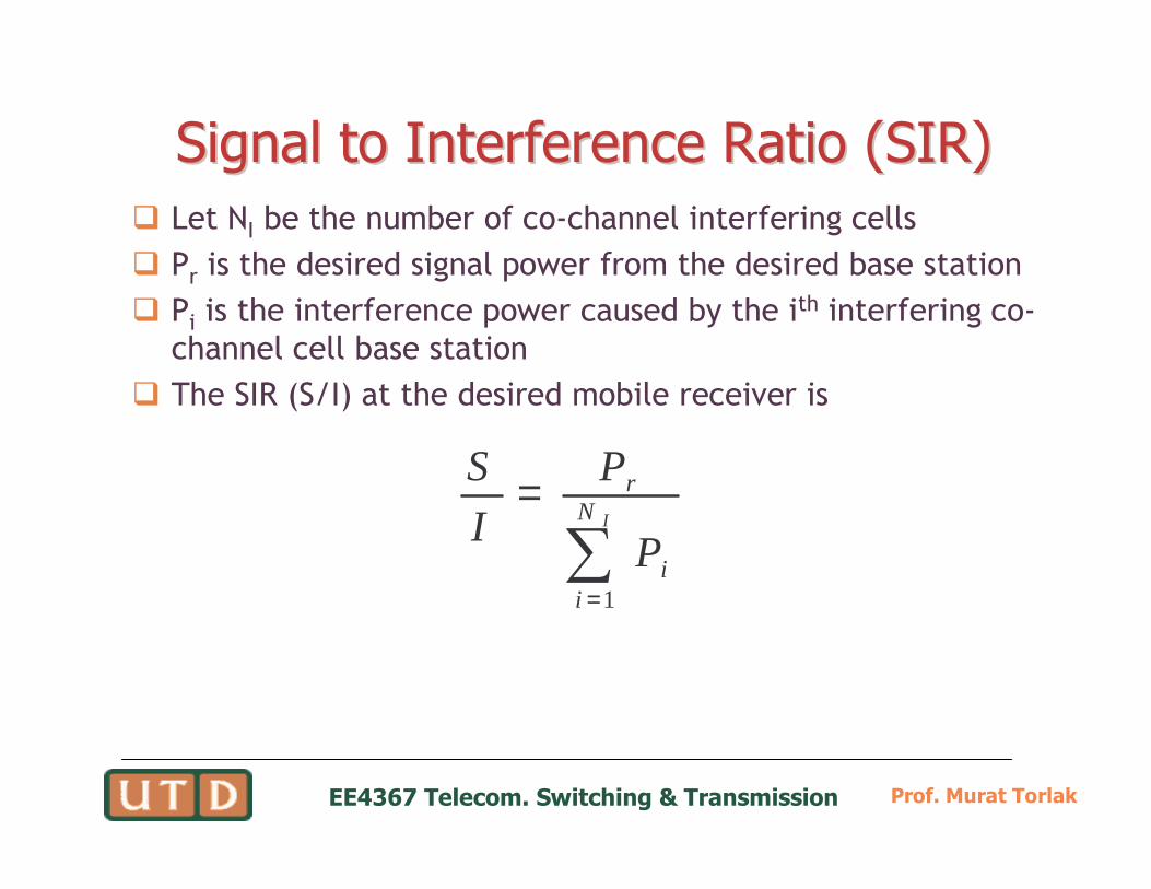
Signal to Interference Ratio (SIR)Signal to Interference Ratio (SIR)

� Let NI be the number of co-channel interfering cells

� Pr is the desired signal power from the desired base station

� Pi is the interference power caused by the ith interfering co-

channel cell base station

� The SIR (S/I) at the desired mobile receiver is

1

I

rN

ii

S P

IP

=

=∑


Recall PowerRecall Power--Distance RelationDistance Relation

� Average received signal strength at any point in a mobile

radio channel is

� If d0 is the close-in reference point in the far field region of

the antenna from the transmitting antenna

� Pt is the transmitter power

� γ is the path loss exponent

� Pr is the received power at a distance d

0r t

dP PK

d

γ−

=


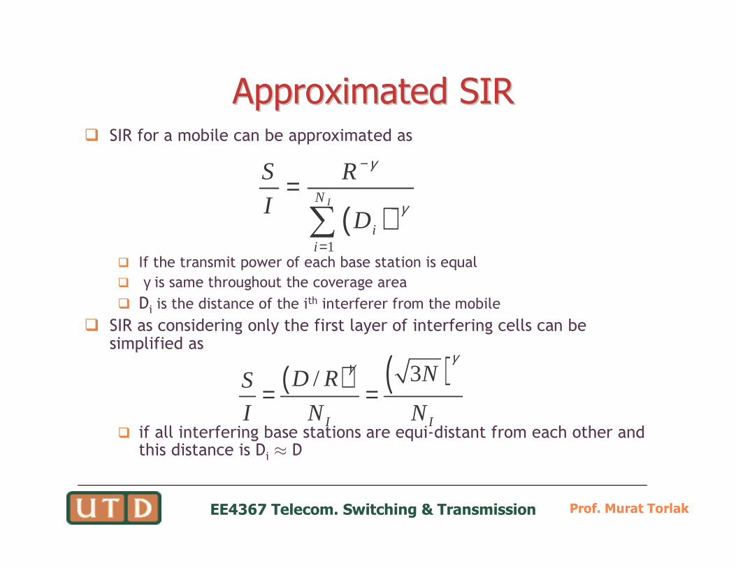
Approximated SIRApproximated SIR� SIR for a mobile can be approximated as

� If the transmit power of each base station is equal

� γ is same throughout the coverage area

� Di is the distance of the ith interferer from the mobile

� SIR as considering only the first layer of interfering cells can be simplified as

� if all interfering base stations are equi-distant from each other and this distance is Di ≈ D

( )1

IN

ii

S R

ID

γ

γ

−

−

=

=∑

( ) ( )3/

I I

ND RS

I N N

γγ

= =


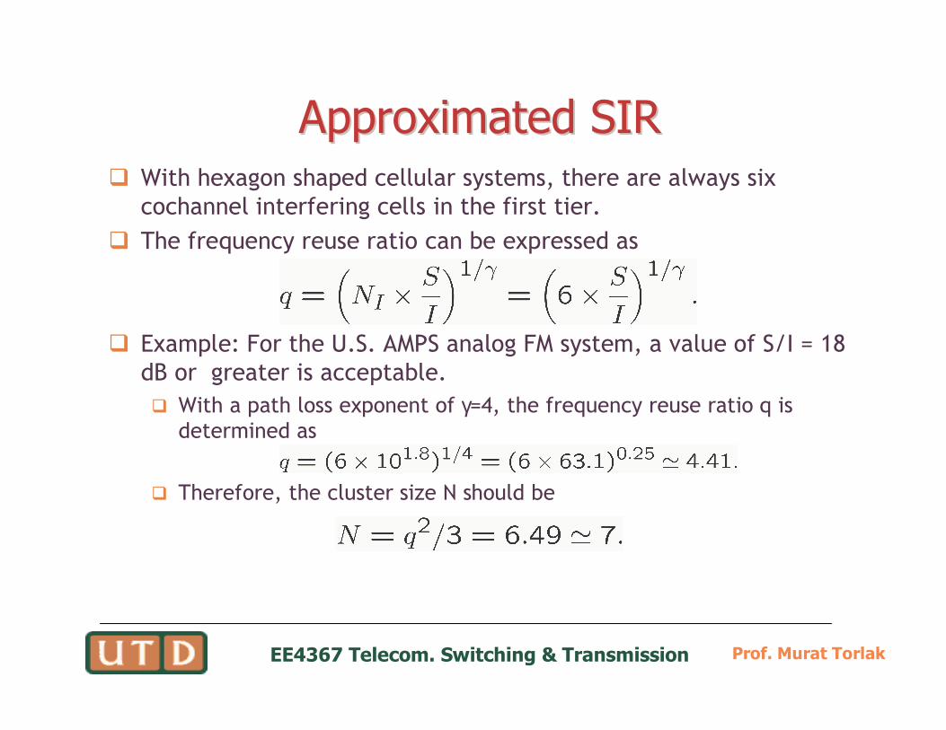
Approximated SIRApproximated SIR� With hexagon shaped cellular systems, there are always six

cochannel interfering cells in the first tier.

� The frequency reuse ratio can be expressed as

� Example: For the U.S. AMPS analog FM system, a value of S/I = 18

dB or greater is acceptable.

� With a path loss exponent of γ=4, the frequency reuse ratio q is

determined as

� Therefore, the cluster size N should be


S/I Ratio S/I Ratio vsvs Cluster SizeCluster Size

� Suppose the acceptable S/I in a cellular system is 20 dB.

� γ=4, what is the minimum cluster size? Consider only the

closest interferers.

Documents

Path Loss - Laboratório de Comunicações e Sinaisablima/grad/tfm/slides/Torlak/...EE4367 Telecom. Switching & Transmission Prof. Murat Torlak Linear Path Loss Suppose s(t) of power