Patch Test Calibration

01/05/2014

with NaviModel

01/05/2014

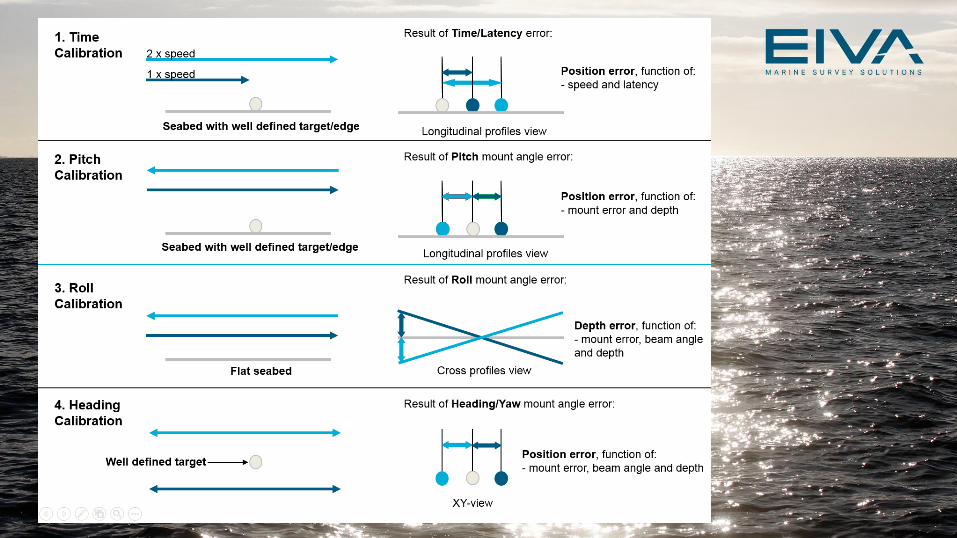
A multibeam Patch Test calibration serves a dual purpose:

a. To determine the mount angles of the multibeam transducer

relative to the three axes of the local coordinate system of the

vessel/ROV. These three figures are often referred to as the roll-,

pitch- and heading mount angles.

b. To confirm the relationship between the time-tagging on the

multibeam data and the time-tagging on the position data. This

figure is often referred to as the latency or as the time value.

Patch Test – Purpose of the Calibration

Bearing in mind the purpose of a Patch Test, it is necessary, prior to the calibration, to:

a. Calibrate relevant sensors (gyro, motion) relative to the local coordinate system of the

vessel/gyro.

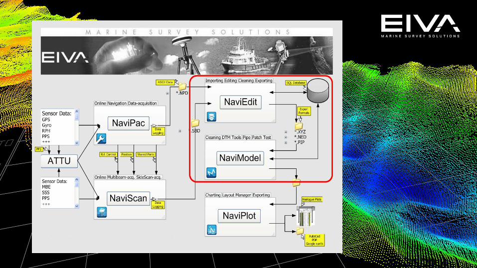
b. Configure NaviPac/NaviScan as well as the multibeam echo-sounder to correctly utilize the

same, accurate time reference for the time-tagging of the various sensor data.

Patch Test – Prior to the Calibration

To enable the values to be isolated and quantified, some pre-defined datasets in specific patterns must first be collected and then processed in a given sequence. The recommended sequence of Patch Test processing is:

• Time.

• Pitch.

• Roll.

• Heading.

Patch Test – Sequence in Processing

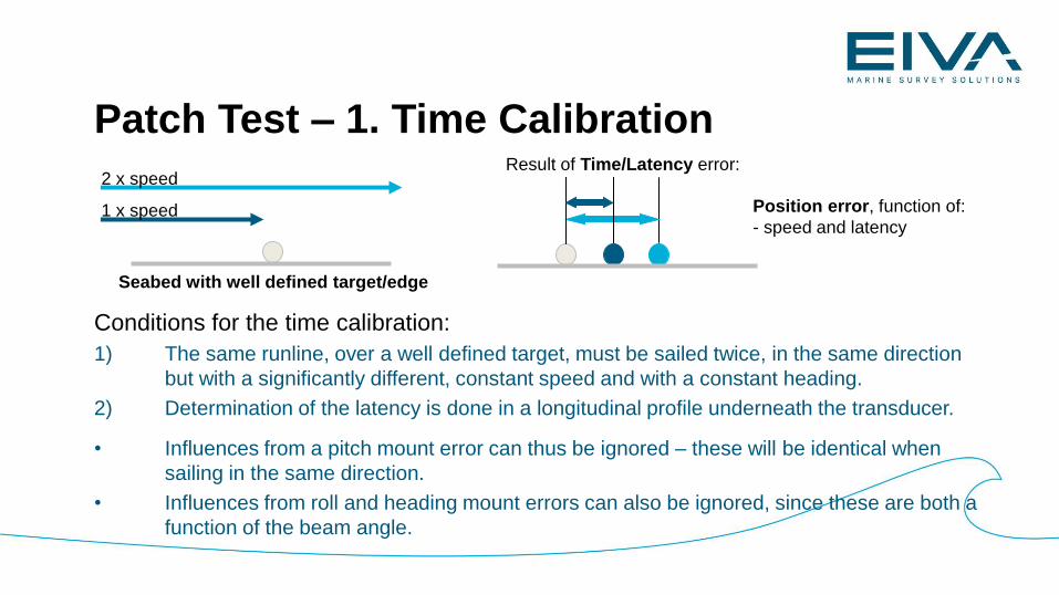
Conditions for the time calibration:

1) The same runline, over a well defined target, must be sailed twice, in the same direction

but with a significantly different, constant speed and with a constant heading.

2) Determination of the latency is done in a longitudinal profile underneath the transducer.

• Influences from a pitch mount error can thus be ignored – these will be identical when

sailing in the same direction.

• Influences from roll and heading mount errors can also be ignored, since these are both a

function of the beam angle.

Patch Test – 1. Time Calibration

Seabed with well defined target/edge

2 x speed

1 x speed

Result of Time/Latency error:

Position error, function of:

- speed and latency

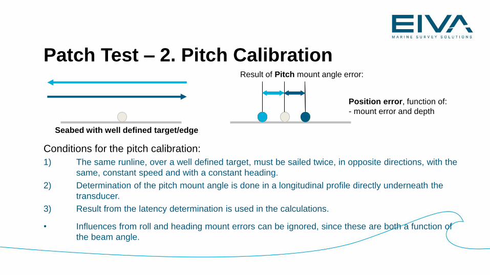
Conditions for the pitch calibration:

1) The same runline, over a well defined target, must be sailed twice, in opposite directions, with the

same, constant speed and with a constant heading.

2) Determination of the pitch mount angle is done in a longitudinal profile directly underneath the

transducer.

3) Result from the latency determination is used in the calculations.

• Influences from roll and heading mount errors can be ignored, since these are both a function of

the beam angle.

Patch Test – 2. Pitch CalibrationResult of Pitch mount angle error:

Seabed with well defined target/edge

Position error, function of:

- mount error and depth

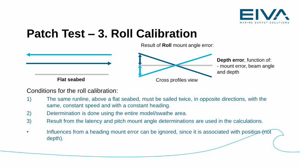
Conditions for the roll calibration:

1) The same runline, above a flat seabed, must be sailed twice, in opposite directions, with the

same, constant speed and with a constant heading.

2) Determination is done using the entire model/swathe area.

3) Result from the latency and pitch mount angle determinations are used in the calculations.

• Influences from a heading mount error can be ignored, since it is associated with position (not

depth).

Patch Test – 3. Roll Calibration Result of Roll mount angle error:

Cross profiles view

Depth error, function of:

- mount error, beam angle

and depth

Flat seabed

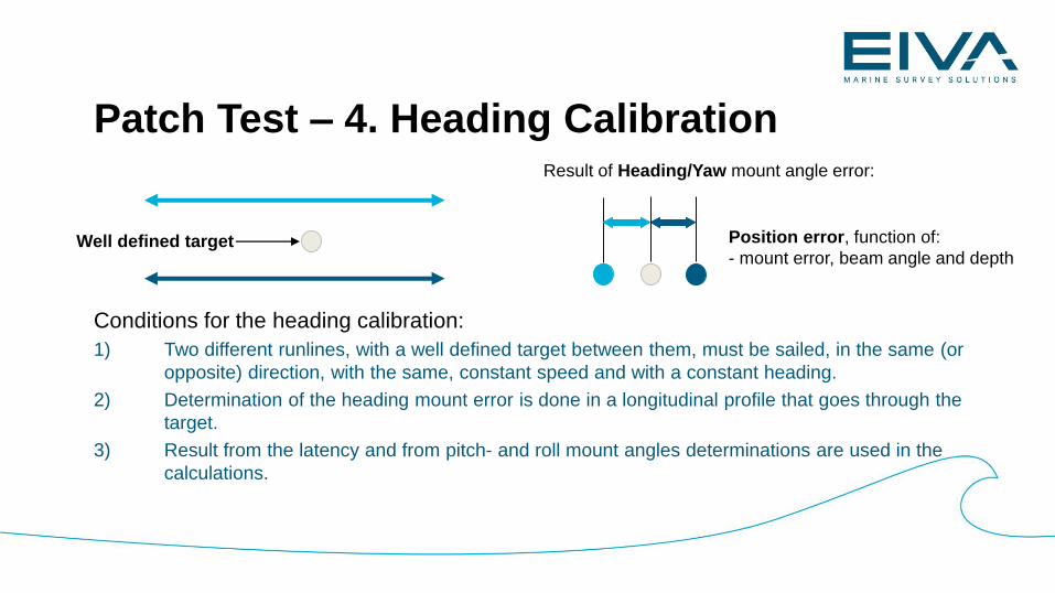
Conditions for the heading calibration:

1) Two different runlines, with a well defined target between them, must be sailed, in the same (or

opposite) direction, with the same, constant speed and with a constant heading.

2) Determination of the heading mount error is done in a longitudinal profile that goes through the

target.

3) Result from the latency and from pitch- and roll mount angles determinations are used in the

calculations.

Patch Test – 4. Heading Calibration

Well defined target

Result of Heading/Yaw mount angle error:

Position error, function of:

- mount error, beam angle and depth

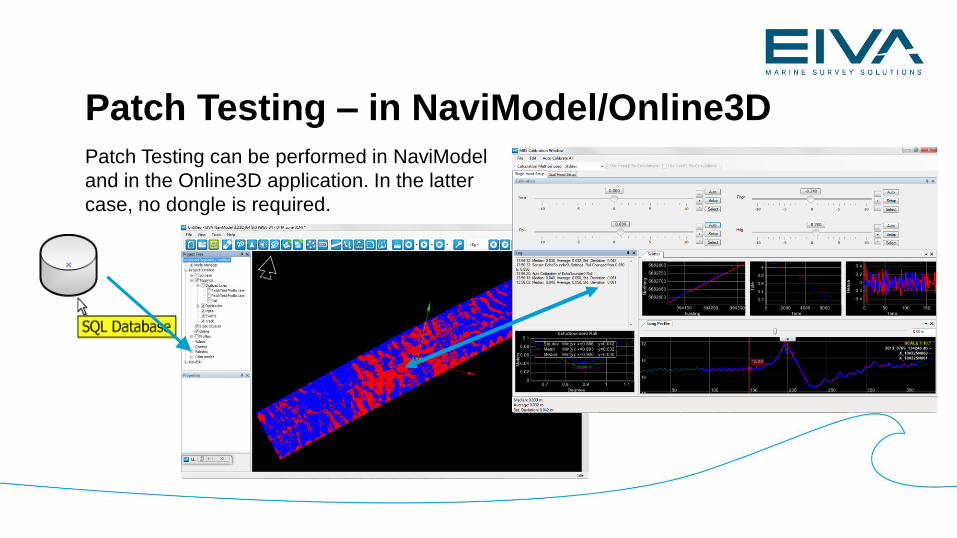
Patch Testing – in NaviModel/Online3DPatch Testing can be performed in NaviModel

and in the Online3D application. In the latter

case, no dongle is required.

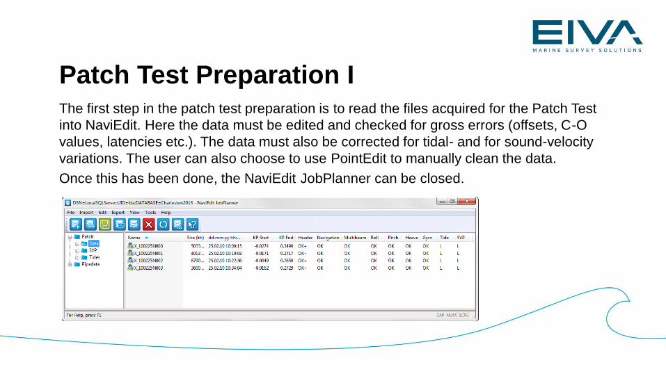
The first step in the patch test preparation is to read the files acquired for the Patch Test

into NaviEdit. Here the data must be edited and checked for gross errors (offsets, C-O

values, latencies etc.). The data must also be corrected for tidal- and for sound-velocity

variations. The user can also choose to use PointEdit to manually clean the data.

Once this has been done, the NaviEdit JobPlanner can be closed.

Patch Test Preparation I

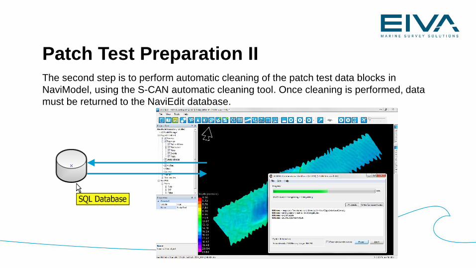
The second step is to perform automatic cleaning of the patch test data blocks in

NaviModel, using the S-CAN automatic cleaning tool. Once cleaning is performed, data

must be returned to the NaviEdit database.

Patch Test Preparation II

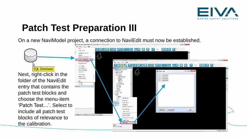
On a new NaviModel project, a connection to NaviEdit must now be established.

Patch Test Preparation III

Next, right-click in the

folder of the NaviEdit

entry that contains the

patch test blocks and

choose the menu-item

‘Patch Test…’. Select to

include all patch test

blocks of relevance to

the calibration.

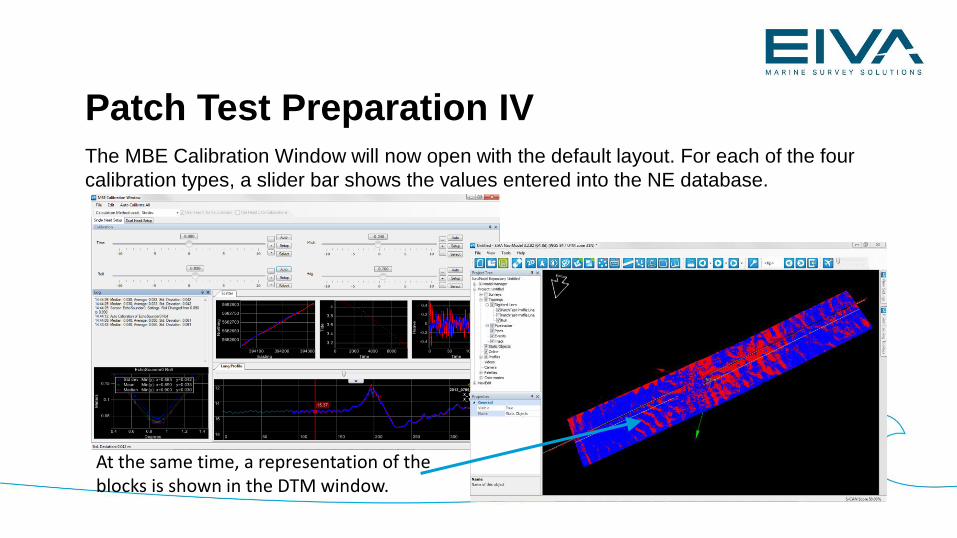
The MBE Calibration Window will now open with the default layout. For each of the four

calibration types, a slider bar shows the values entered into the NE database.

Patch Test Preparation IV

At the same time, a representation of the blocks is shown in the DTM window.

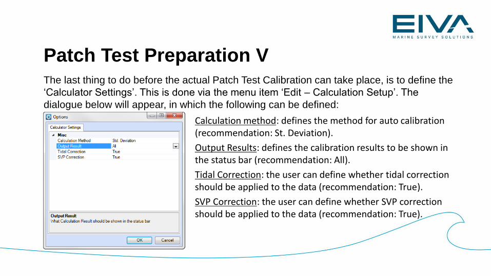
The last thing to do before the actual Patch Test Calibration can take place, is to define the

‘Calculator Settings’. This is done via the menu item ‘Edit – Calculation Setup’. The

dialogue below will appear, in which the following can be defined:

Patch Test Preparation V

Calculation method: defines the method for auto calibration (recommendation: St. Deviation).

Output Results: defines the calibration results to be shown in the status bar (recommendation: All).

Tidal Correction: the user can define whether tidal correction should be applied to the data (recommendation: True).

SVP Correction: the user can define whether SVP correction should be applied to the data (recommendation: True).

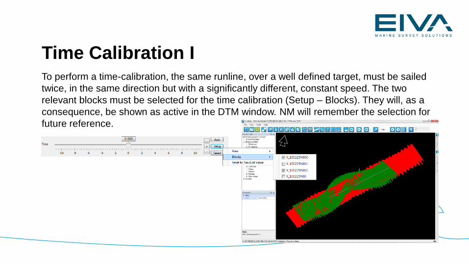
To perform a time-calibration, the same runline, over a well defined target, must be sailed

twice, in the same direction but with a significantly different, constant speed. The two

relevant blocks must be selected for the time calibration (Setup – Blocks). They will, as a

consequence, be shown as active in the DTM window. NM will remember the selection for

future reference.

Time Calibration I

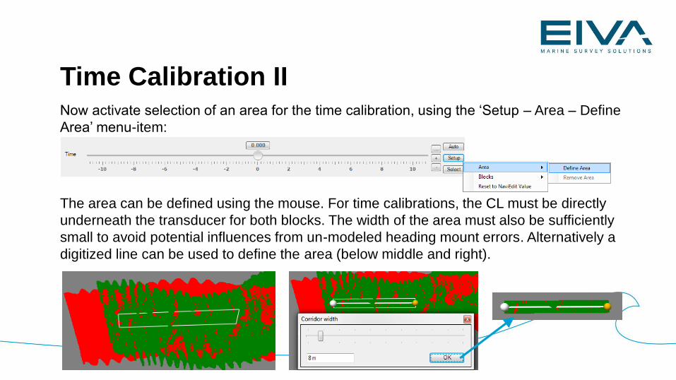
Time Calibration IINow activate selection of an area for the time calibration, using the ‘Setup – Area – Define

Area’ menu-item:

The area can be defined using the mouse. For time calibrations, the CL must be directly

underneath the transducer for both blocks. The width of the area must also be sufficiently

small to avoid potential influences from un-modeled heading mount errors. Alternatively a

digitized line can be used to define the area (below middle and right).

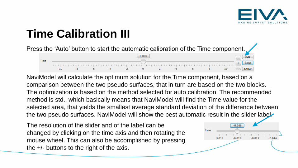
Press the ‘Auto’ button to start the automatic calibration of the Time component.

NaviModel will calculate the optimum solution for the Time component, based on a

comparison between the two pseudo surfaces, that in turn are based on the two blocks.

The optimization is based on the method selected for auto calibration. The recommended

method is std., which basically means that NaviModel will find the Time value for the

selected area, that yields the smallest average standard deviation of the difference between

the two pseudo surfaces. NaviModel will show the best automatic result in the slider label.

The resolution of the slider and of the label can be

changed by clicking on the time axis and then rotating the

mouse wheel. This can also be accomplished by pressing

the +/- buttons to the right of the axis.

Time Calibration III

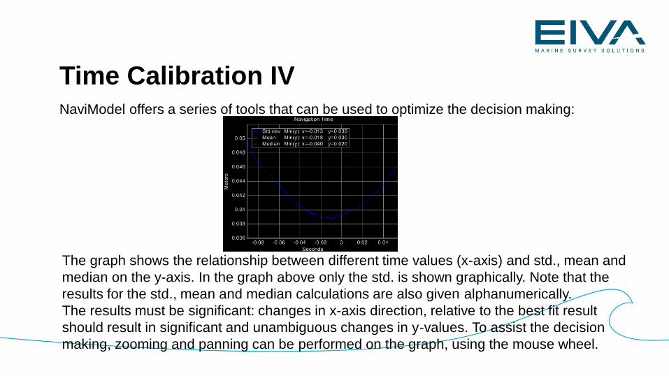
NaviModel offers a series of tools that can be used to optimize the decision making:

Time Calibration IV

The graph shows the relationship between different time values (x-axis) and std., mean and

median on the y-axis. In the graph above only the std. is shown graphically. Note that the

results for the std., mean and median calculations are also given alphanumerically.

The results must be significant: changes in x-axis direction, relative to the best fit result

should result in significant and unambiguous changes in y-values. To assist the decision

making, zooming and panning can be performed on the graph, using the mouse wheel.

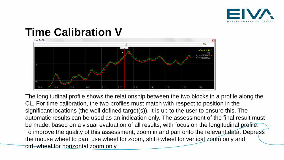
The longitudinal profile shows the relationship between the two blocks in a profile along the

CL. For time calibration, the two profiles must match with respect to position in the

significant locations (the well defined target(s)). It is up to the user to ensure this. The

automatic results can be used as an indication only. The assessment of the final result must

be made, based on a visual evaluation of all results, with focus on the longitudinal profile.

To improve the quality of this assessment, zoom in and pan onto the relevant data. Depress

the mouse wheel to pan, use wheel for zoom, shift+wheel for vertical zoom only and

ctrl+wheel for horizontal zoom only.

Time Calibration V

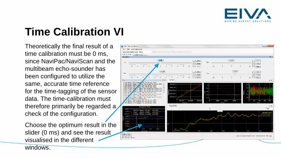
Theoretically the final result of a

time calibration must be 0 ms,

since NaviPac/NaviScan and the

multibeam echo-sounder has

been configured to utilize the

same, accurate time reference

for the time-tagging of the sensor

data. The time-calibration must

therefore primarily be regarded a

check of the configuration.

Choose the optimum result in the

slider (0 ms) and see the result

visualised in the different

windows.

Time Calibration VI

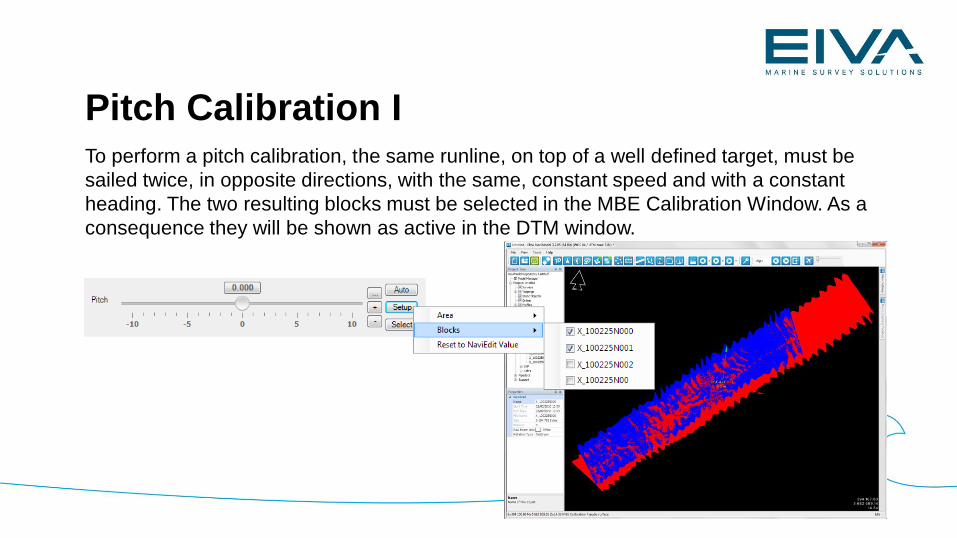
To perform a pitch calibration, the same runline, on top of a well defined target, must be

sailed twice, in opposite directions, with the same, constant speed and with a constant

heading. The two resulting blocks must be selected in the MBE Calibration Window. As a

consequence they will be shown as active in the DTM window.

Pitch Calibration I

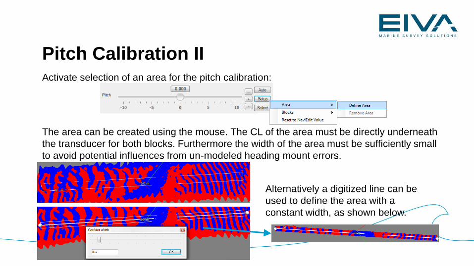
Activate selection of an area for the pitch calibration:

The area can be created using the mouse. The CL of the area must be directly underneath

the transducer for both blocks. Furthermore the width of the area must be sufficiently small

to avoid potential influences from un-modeled heading mount errors.

Pitch Calibration II

Alternatively a digitized line can be

used to define the area with a

constant width, as shown below.

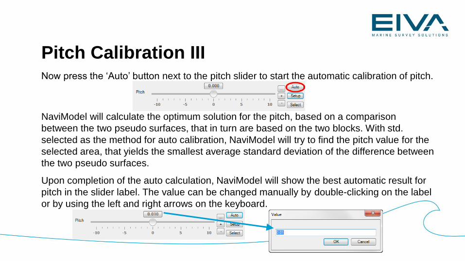
Now press the ‘Auto’ button next to the pitch slider to start the automatic calibration of pitch.

NaviModel will calculate the optimum solution for the pitch, based on a comparison

between the two pseudo surfaces, that in turn are based on the two blocks. With std.

selected as the method for auto calibration, NaviModel will try to find the pitch value for the

selected area, that yields the smallest average standard deviation of the difference between

the two pseudo surfaces.

Upon completion of the auto calculation, NaviModel will show the best automatic result for

pitch in the slider label. The value can be changed manually by double-clicking on the label

or by using the left and right arrows on the keyboard.

Pitch Calibration III

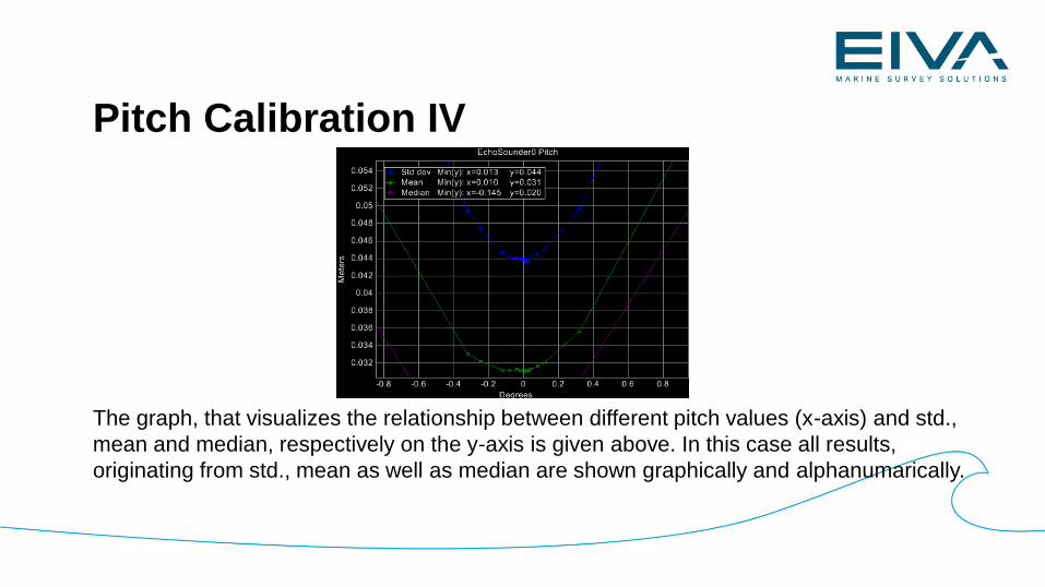
Pitch Calibration IV

The graph, that visualizes the relationship between different pitch values (x-axis) and std.,

mean and median, respectively on the y-axis is given above. In this case all results,

originating from std., mean as well as median are shown graphically and alphanumarically.

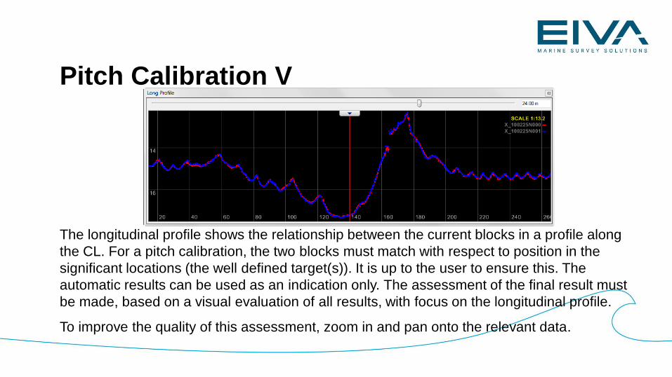
Pitch Calibration V

The longitudinal profile shows the relationship between the current blocks in a profile along

the CL. For a pitch calibration, the two blocks must match with respect to position in the

significant locations (the well defined target(s)). It is up to the user to ensure this. The

automatic results can be used as an indication only. The assessment of the final result must

be made, based on a visual evaluation of all results, with focus on the longitudinal profile.

To improve the quality of this assessment, zoom in and pan onto the relevant data.

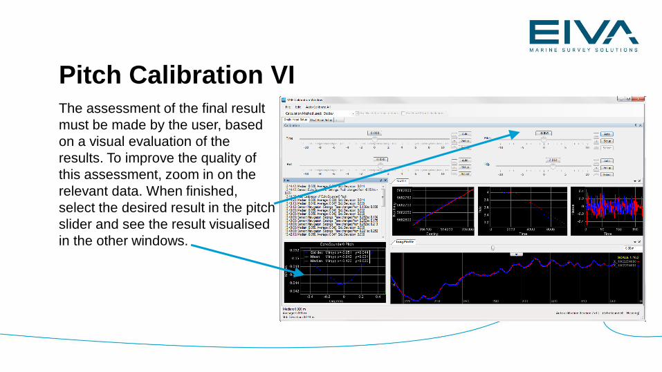
The assessment of the final result

must be made by the user, based

on a visual evaluation of the

results. To improve the quality of

this assessment, zoom in on the

relevant data. When finished,

select the desired result in the pitch

slider and see the result visualised

in the other windows.

Pitch Calibration VI

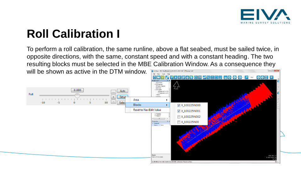
To perform a roll calibration, the same runline, above a flat seabed, must be sailed twice, in

opposite directions, with the same, constant speed and with a constant heading. The two

resulting blocks must be selected in the MBE Calibration Window. As a consequence they

will be shown as active in the DTM window.

Roll Calibration I

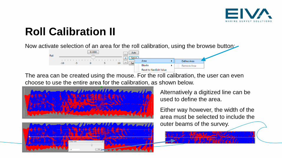
Roll Calibration IINow activate selection of an area for the roll calibration, using the browse button:

The area can be created using the mouse. For the roll calibration, the user can even

choose to use the entire area for the calibration, as shown below.

Alternatively a digitized line can be

used to define the area.

Either way however, the width of the

area must be selected to include the

outer beams of the survey.

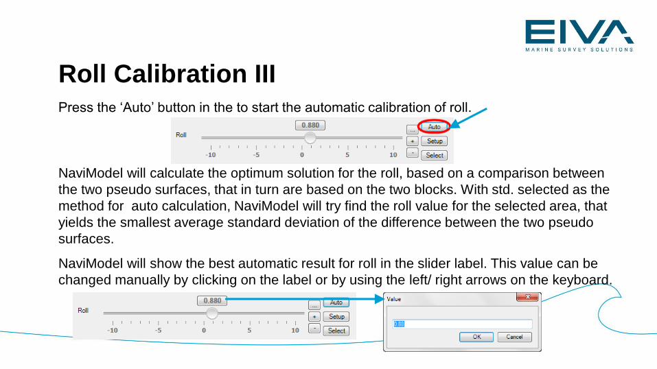
Roll Calibration IIIPress the ‘Auto’ button in the to start the automatic calibration of roll.

NaviModel will calculate the optimum solution for the roll, based on a comparison between

the two pseudo surfaces, that in turn are based on the two blocks. With std. selected as the

method for auto calculation, NaviModel will try find the roll value for the selected area, that

yields the smallest average standard deviation of the difference between the two pseudo

surfaces.

NaviModel will show the best automatic result for roll in the slider label. This value can be

changed manually by clicking on the label or by using the left/ right arrows on the keyboard.

Roll Calibration IV

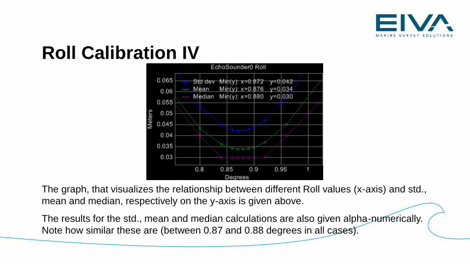
The graph, that visualizes the relationship between different Roll values (x-axis) and std.,

mean and median, respectively on the y-axis is given above.

The results for the std., mean and median calculations are also given alpha-numerically.

Note how similar these are (between 0.87 and 0.88 degrees in all cases).

Roll Calibration V

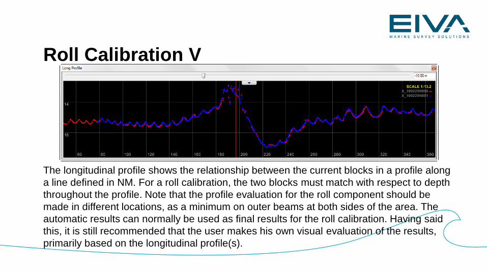
The longitudinal profile shows the relationship between the current blocks in a profile along

a line defined in NM. For a roll calibration, the two blocks must match with respect to depth

throughout the profile. Note that the profile evaluation for the roll component should be

made in different locations, as a minimum on outer beams at both sides of the area. The

automatic results can normally be used as final results for the roll calibration. Having said

this, it is still recommended that the user makes his own visual evaluation of the results,

primarily based on the longitudinal profile(s).

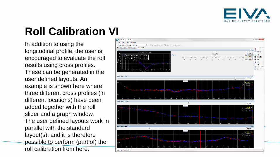
Roll Calibration VIIn addition to using the

longitudinal profile, the user is

encouraged to evaluate the roll

results using cross profiles.

These can be generated in the

user defined layouts. An

example is shown here where

three different cross profiles (in

different locations) have been

added together with the roll

slider and a graph window.

The user defined layouts work in

parallel with the standard

layout(s), and it is therefore

possible to perform (part of) the

roll calibration from here.

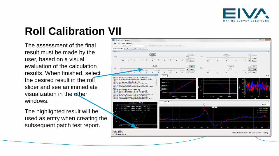
Roll Calibration VIIThe assessment of the final

result must be made by the

user, based on a visual

evaluation of the calculation

results. When finished, select

the desired result in the roll

slider and see an immediate

visualization in the other

windows.

The highlighted result will be

used as entry when creating the

subsequent patch test report.

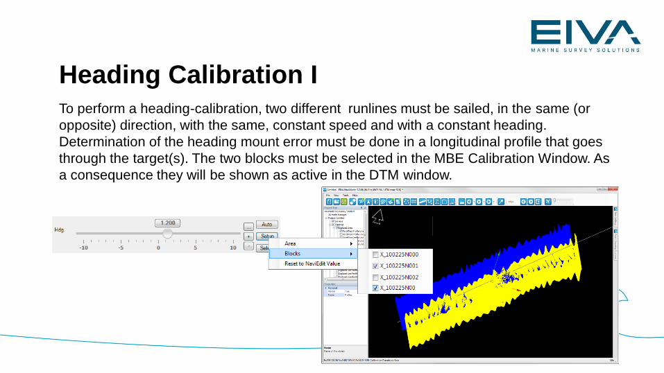
Heading Calibration ITo perform a heading-calibration, two different runlines must be sailed, in the same (or

opposite) direction, with the same, constant speed and with a constant heading.

Determination of the heading mount error must be done in a longitudinal profile that goes

through the target(s). The two blocks must be selected in the MBE Calibration Window. As

a consequence they will be shown as active in the DTM window.

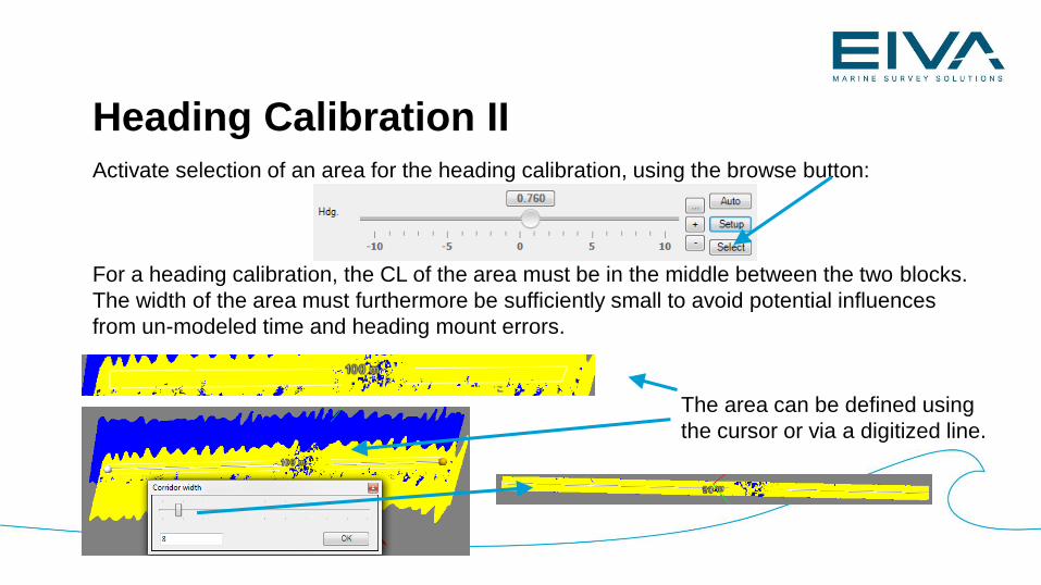
Activate selection of an area for the heading calibration, using the browse button:

For a heading calibration, the CL of the area must be in the middle between the two blocks.

The width of the area must furthermore be sufficiently small to avoid potential influences

from un-modeled time and heading mount errors.

Heading Calibration II

The area can be defined using

the cursor or via a digitized line.

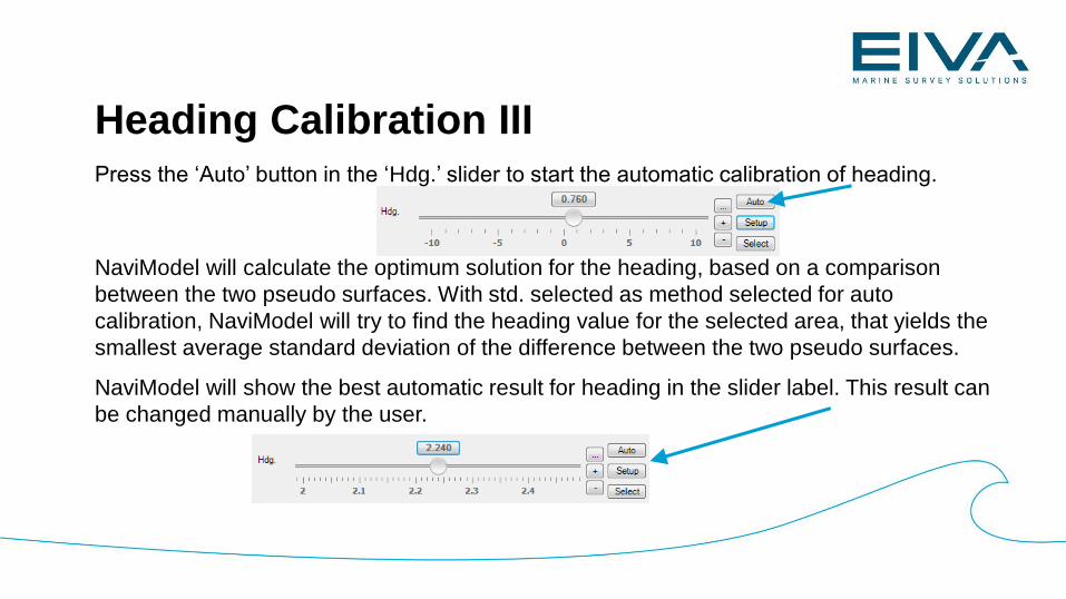
Heading Calibration IIIPress the ‘Auto’ button in the ‘Hdg.’ slider to start the automatic calibration of heading.

NaviModel will calculate the optimum solution for the heading, based on a comparison

between the two pseudo surfaces. With std. selected as method selected for auto

calibration, NaviModel will try to find the heading value for the selected area, that yields the

smallest average standard deviation of the difference between the two pseudo surfaces.

NaviModel will show the best automatic result for heading in the slider label. This result can

be changed manually by the user.

Heading Calibration IV

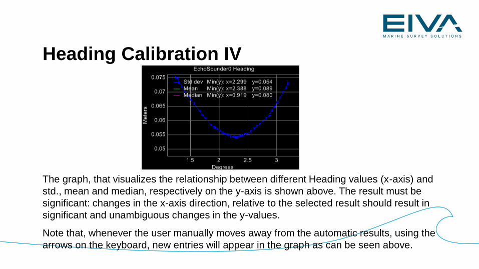
The graph, that visualizes the relationship between different Heading values (x-axis) and

std., mean and median, respectively on the y-axis is shown above. The result must be

significant: changes in the x-axis direction, relative to the selected result should result in

significant and unambiguous changes in the y-values.

Note that, whenever the user manually moves away from the automatic results, using the

arrows on the keyboard, new entries will appear in the graph as can be seen above.

Heading Calibration V

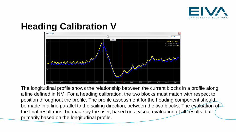
The longitudinal profile shows the relationship between the current blocks in a profile along

a line defined in NM. For a heading calibration, the two blocks must match with respect to

position throughout the profile. The profile assessment for the heading component should

be made in a line parallel to the sailing direction, between the two blocks. The evaluation of

the final result must be made by the user, based on a visual evaluation of all results, but

primarily based on the longitudinal profile.

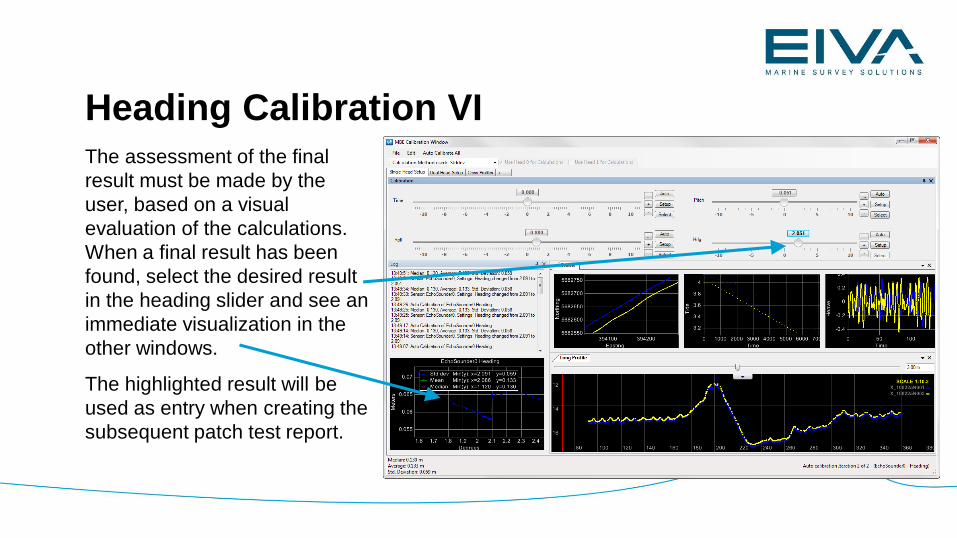
Heading Calibration VIThe assessment of the final

result must be made by the

user, based on a visual

evaluation of the calculations.

When a final result has been

found, select the desired result

in the heading slider and see an

immediate visualization in the

other windows.

The highlighted result will be

used as entry when creating the

subsequent patch test report.

Iterations IIt is often difficult to totally isolate influences from other sources (not constant speed,

varying heading, noisy positioning etc.) when conducting a calculation. So therefore it is

recommended to re-iterate the calibration calculations, with the obtained mount angles and

the latency value from the first iteration, in order to investigate whether an additional fine-

tuning is required.

This is easily accomplished in NaviModel. The Patch Test tool facilitates a function to

perform auto calibration in a number of iterations, the ‘Auto Calibrate All’ function. ‘Auto

Calibrate All’ takes advantage of the fact that once the blocks and areas have been defined,

they will be remembered by the Patch Test tool.

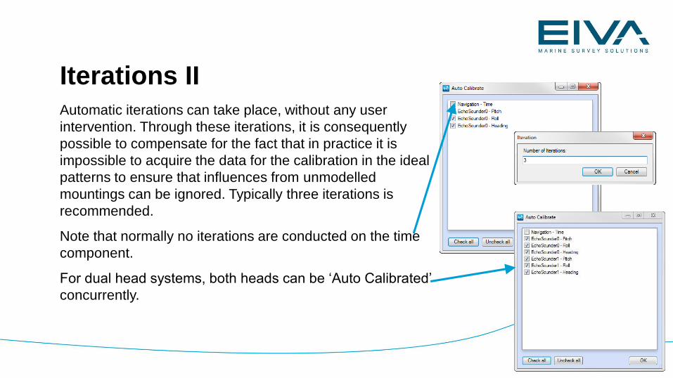
Iterations IIAutomatic iterations can take place, without any user

intervention. Through these iterations, it is consequently

possible to compensate for the fact that in practice it is

impossible to acquire the data for the calibration in the ideal

patterns to ensure that influences from unmodelled

mountings can be ignored. Typically three iterations is

recommended.

Note that normally no iterations are conducted on the time

component.

For dual head systems, both heads can be ‘Auto Calibrated’

concurrently.

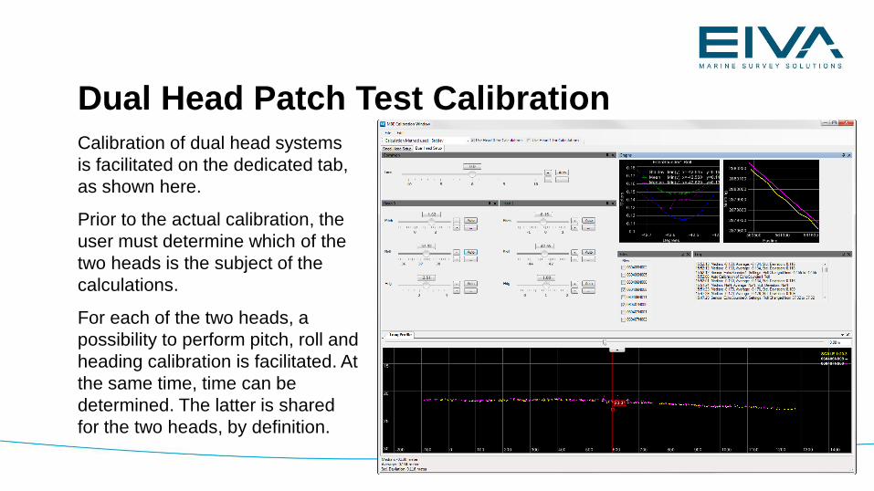
Dual Head Patch Test Calibration Calibration of dual head systems

is facilitated on the dedicated tab,

as shown here.

Prior to the actual calibration, the

user must determine which of the

two heads is the subject of the

calculations.

For each of the two heads, a

possibility to perform pitch, roll and

heading calibration is facilitated. At

the same time, time can be

determined. The latter is shared

for the two heads, by definition.

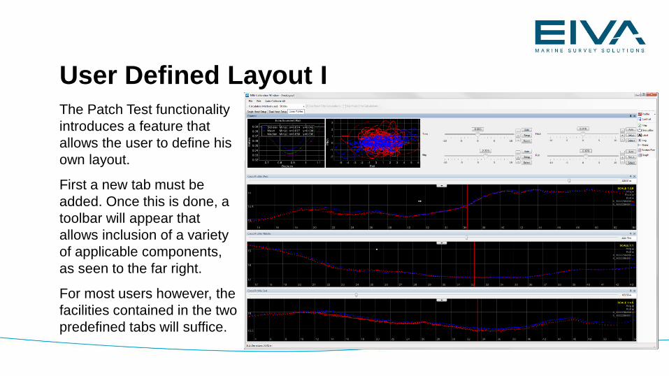
User Defined Layout IThe Patch Test functionality

introduces a feature that

allows the user to define his

own layout.

First a new tab must be

added. Once this is done, a

toolbar will appear that

allows inclusion of a variety

of applicable components,

as seen to the far right.

For most users however, the

facilities contained in the two

predefined tabs will suffice.

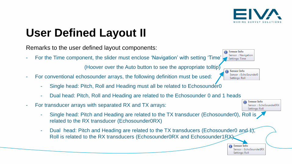
User Defined Layout IIRemarks to the user defined layout components:

- For the Time component, the slider must enclose ‘Navigation’ with setting ‘Time’

(Hoover over the Auto button to see the appropriate tolltip)

- For conventional echosounder arrays, the following definition must be used:

- Single head: Pitch, Roll and Heading must all be related to Echosounder0

- Dual head: Pitch, Roll and Heading are related to the Echosounder 0 and 1 heads

- For transducer arrays with separated RX and TX arrays:

- Single head: Pitch and Heading are related to the TX transducer (Echosounder0), Roll is

related to the RX transducer (Echosounder0RX)

- Dual head: Pitch and Heading are related to the TX transducers (Echosounder0 and 1),

Roll is related to the RX transducers (Echosounder0RX and Echosounder1RX)

Save and Load LayoutThe Layouts can be saved using the ‘File – Save Layout’ menu item. The saved layouts

can be used again thorugh the use of the ‘Load Layout’ menu option.

The saved layout will contain configuration information related to all tabs that were

created at the time of saving.

The ‘Restore Default Layout’ functionality will restore to factory defaults with respect to

layout. As a consequense of this action, any present customer layout tabs will be

removed.

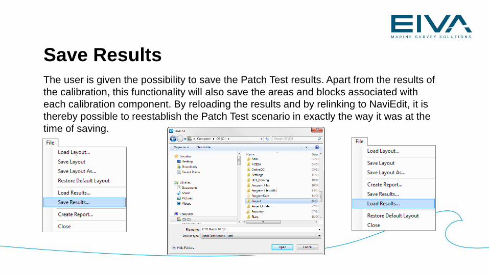
Save ResultsThe user is given the possibility to save the Patch Test results. Apart from the results of

the calibration, this functionality will also save the areas and blocks associated with

each calibration component. By reloading the results and by relinking to NaviEdit, it is

thereby possible to reestablish the Patch Test scenario in exactly the way it was at the

time of saving.

Using the Patch Test results in NaviScan

The saved Patch Test results file can be loaded into the NaviScan Config program. The

parameters will subsequently be used in NaviScan online acquisition and visualization

and consequently saved with the raw SBD-files.

When loading the parameters, the user is instructed that NaviScan will not apply the

time value, even if it differs from 0 in the result file, since it is recommended to use 0 as

time value. If the desire is to use a value that differs from 0, the value must be entered

manually.

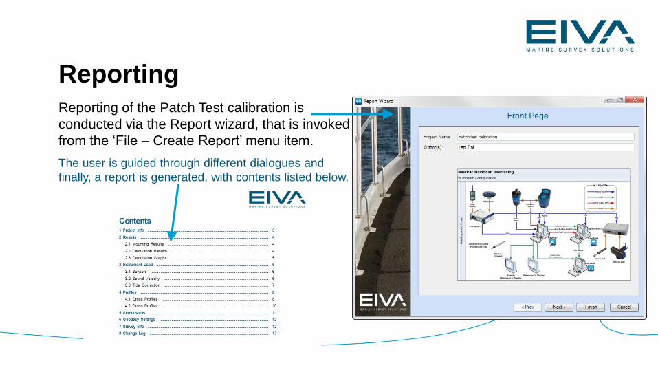
ReportingReporting of the Patch Test calibration is

conducted via the Report wizard, that is invoked

from the ‘File – Create Report’ menu item.

The user is guided through different dialogues and

finally, a report is generated, with contents listed below.

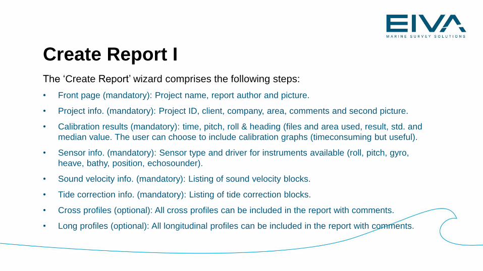
Create Report IThe ‘Create Report’ wizard comprises the following steps:

• Front page (mandatory): Project name, report author and picture.

• Project info. (mandatory): Project ID, client, company, area, comments and second picture.

• Calibration results (mandatory): time, pitch, roll & heading (files and area used, result, std. and

median value. The user can choose to include calibration graphs (timeconsuming but useful).

• Sensor info. (mandatory): Sensor type and driver for instruments available (roll, pitch, gyro,

heave, bathy, position, echosounder).

• Sound velocity info. (mandatory): Listing of sound velocity blocks.

• Tide correction info. (mandatory): Listing of tide correction blocks.

• Cross profiles (optional): All cross profiles can be included in the report with comments.

• Long profiles (optional): All longitudinal profiles can be included in the report with comments.

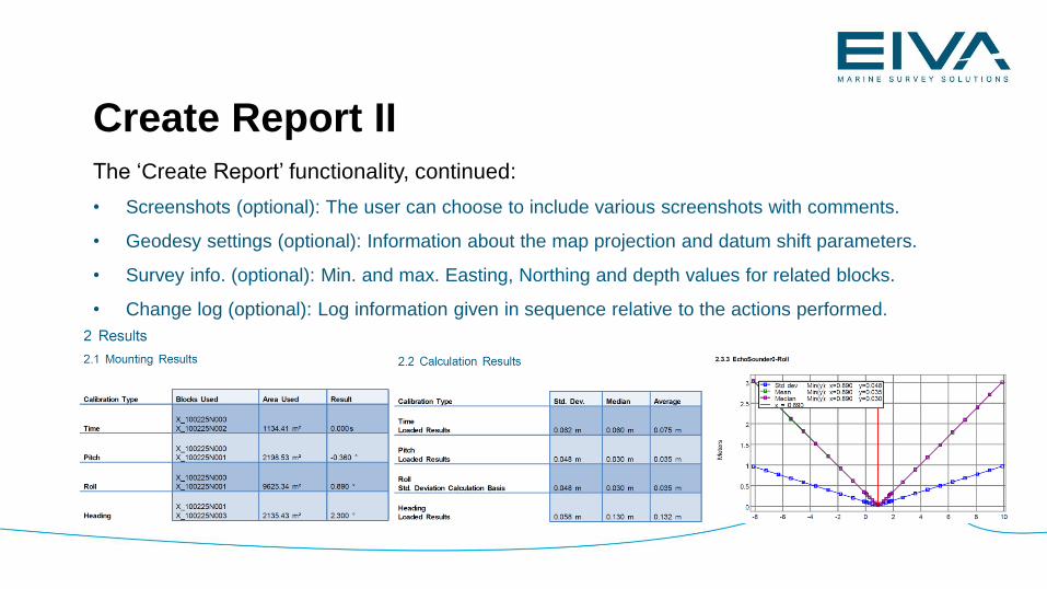
Create Report IIThe ‘Create Report’ functionality, continued:

• Screenshots (optional): The user can choose to include various screenshots with comments.

• Geodesy settings (optional): Information about the map projection and datum shift parameters.

• Survey info. (optional): Min. and max. Easting, Northing and depth values for related blocks.

• Change log (optional): Log information given in sequence relative to the actions performed.