PARTITION OF UNITY ISOGEOMETRIC ANALYSIS FOR SINGULARLYPERTURBED PROBLEMS AND FOURTH ORDER DIFFERENTIAL

EQUATIONS CONTAINING SINGULARITIES

by

Sinae Kim

A dissertation submitted to the faculty ofThe University of North Carolina at Charlotte

in partial fulfillment of the requirementsfor the degree of Doctor of Philosophy in

Applied Mathematics

Charlotte

2016

Approved by:

Dr. Hae-soo Oh

Dr. Joel Avrin

Dr. Shaozhong Deng

Dr. Churlzu Lim

ii

c©2016Sinae Kim

ALL RIGHTS RESERVED

iii

ABSTRACT

SINAE KIM. Partition of Unity Isogeometric Analysis for singularly Perturbedproblems and fourth order differential equations containing singularities. (Under the

direction of DR. HAE-SOO OH)

Our aim in this research is to develop the numerical solutions of singularly per-

turbed convection-diffusion problems and heat equations in a circular domain, and

fourth-order PDEs containing singularities, avoiding fine mesh around the boundary

layer or singular zone. To resolve the oscillations of classical numerical solutions of our

problems, we construct boundary layer elements via boundary layer analysis for the

perturbed problem. We also construct singular functions by the known solution on

the crack domain for the fourth-order equations containing singularities. We modify

the boundary layer elements and singular functions using partition of unity function

with flat-top, which absorb the boundary layer or crack singularities and do not affect

outside the boundary layer zone or singular zone. Using B-spline Isogeometric Finite

element space enriched with the boundary layer elements and singular functions, we

obtain an accurate numerical scheme on the exact geometry, in a circular domain. As

for the perturbed problems, we develop the boundary layer element on the reference

domain through the geometry mapping which can capture the boundary layer sin-

gularity. As for the fourth-order equations containing singularities, since we already

know the singular functions on the physical domain not reference domain, we add

the singular functions directly or introduce the Mapping Method to generate those

singular functions. We obtain an accurate numerical methods in IGA setting, using

partition of unity functions and enrichment functions.

iv

ACKNOWLEDGMENTS

v

TABLE OF CONTENTS

LIST OF FIGURES vii

LIST OF TABLES ix

CHAPTER 1: INTRODUCTION 1

CHAPTER 2: PRELIMINARIES 4

2.1. Isogeometric Analysis 4

2.2. B-splines and NURBS 7

2.3. Refinement 12

2.4. Partition of Unity 17

2.5. Boundary Layer Analysis 25

CHAPTER 3: Partition of Unity Isogeometric Analysis 33

3.1. Error Analysis for PU-IGA 33

3.2. Total cost comparison of PU-IGA to IGA 37

3.3. Galerkin Method of Enriched PU-IGA 41

CHAPTER 4: Singulary perturbed convection-diffusion equations in acircle

44

4.1. Introduction 44

4.2. Geometry Mapping 45

4.3. Boundary Layer Analysis 46

4.4. Approximation via finite elements 49

4.5. Numerical Method 50

4.6. Singulary perturbed convection-diffusion equation on an ellipsedomain

73

vi

CHAPTER 5: Singularly perturbed parabolic equation in a circle 76

5.1. Introduction 76

5.2. Discretization 78

5.3. Boundary Layer Analysis 79

5.4. Error Estimates for fully discrete approximations 81

5.5. Numerical Simulations 82

CHAPTER 6: Fourth Order Elliptic Equations containing singularities 87

6.1. Introduction 87

6.2. Enriched PU-IGA and PU-IGA with Mapping Method 90

6.3. Numerical Results 107

6.4. Two-dimensional fourth order elliptic equations on a crackeddisk

112

CHAPTER 7: Conclusion and future directions 126

REFERENCES 128

vii

LIST OF FIGURES

FIGURE 1: NURBS Object 5

FIGURE 2: B-spline Basis 9

FIGURE 3: Knot Insertion 14

FIGURE 4: Order elevation 16

FIGURE 5: k-refinement 18

FIGURE 6: Reference PU 20

FIGURE 7: PU with flat-top 21

FIGURE 8: G Mapping 46

FIGURE 9: periodic 53

FIGURE 10: Patches on Physical Domain 56

FIGURE 11: Patches on reference domain 56

FIGURE 12: 1D convection diffusion Error 62

FIGURE 13: Graphs of numerical solutions obtained by PU-IGA whenε = 10−3(Left) and ε = 10−5(Right).

63

FIGURE 14: (Left) Relative errors in percent when ε = 10−3, a − δ =0.05, b = 0.5, δ = 0.01. (Right) Relative errors in percent when ε =10−4, a− δ = 0.005, b = 0.5, δ = 0.001.

64

FIGURE 15: Schematic diagram of subdomains in the reference domain.Ω1 = [0, a] × [0, 1], Ω2 = [a, 1] × [0, 1], where a = 0.1 and δ = 0.05.The supports of PU functions with flat-top, Ψ1 and Ψ2, are Ω∗1 =[0, a+ δ]× [0, 1] = supp(Ψ1), and Ω∗2 = [a− δ, 1]× [0, 1] = supp(Ψ2).

67

FIGURE 16: Error comparison for different numerical methods 72

FIGURE 17: Ellipse Mapping 73

viii

FIGURE 18: 1D Parabolic error comparison of IGA and Enriched PU-IGA

85

FIGURE 19: 1D Parabolic error comparison of IGA and Enriched PU-IGA

85

FIGURE 20: Relative Error in the Maximum Norm(Left). Conditionnumbers versus degrees freedom in semi log scale (Right).

108

FIGURE 21: Cracked disk and Patches. Ω = Ωsing ∪ Ωreg. 115

FIGURE 22: Computed solution by Mapping method(Left). Computedsolution without mapping method(Right). True solution(Down cen-ter). Figures are computed solutions when B-spline basis functionsof degree p = 5 are used.

124

ix

LIST OF TABLES

TABLE 1: Upper bound of gradient of reference PU 25

TABLE 2: Dominant Balancing 29

TABLE 3: 1D PU-IGA and IGA comparison p-refinement 62

TABLE 4: 1D PU-IGA and IGA comparison h-refinement 63

TABLE 5: 2D convection diffusion error comparison 67

TABLE 6: 2D convection-diffusion on a square 72

TABLE 7: 1D parabolic error comparison for h-refinement 84

TABLE 8: 1D parabolic error comparison for k-refinement 86

TABLE 9: Space Convergence rate 86

TABLE 10: Time convergence rate 86

TABLE 11: 1D Enriched p-refinement of PU-IGA 109

TABLE 12: 1D Enriched k-refinement of PU-IGA 109

TABLE 13: 1D PU-IGA with Mapping Method 110

TABLE 14: 1D IGA for smooth function 113

TABLE 15: 1D condition numbers of smooth solution 113

TABLE 16: 2D PU-IGA with Mapping method for singular fourth-orderequation

125

CHAPTER 1: INTRODUCTION

By Isogeometric Analasis, we can use the design geometry directly for analysis with-

out modifying the geometry for analysis purpose. By using the geometry mapping,

we could approximate the solution on parametric domain for any physical domain.

In Isogeometric Analysis, we use B-spline as the basis functions that allows us to

construct them with any regularity. However, general Isogeometric Analysis does not

give accurate solutions to perturbed problems or fourth-order equations with singu-

larities. Therefore, we enrich Isogeometric Finite Element Space by adding boundary

layer element or singular functions into boundary layer or singular zone using Partion

of Unity with flat-top. We call this approach Partion of Unity Isogeometric Analysis.

(PU-IGA) See [48] and [49]

Most of the numerical methods to solve the singular perturbed problems are based

on domain decomposition or refined meshes near boundary layer in [35], [50], [51],

and [68], etc. In [27], the authors approximated the problem using a quasi-uniform

triangulation and P1 finite element space enriched with boundary layer correctors in

a rectangle and circle. In this paper, we similarly derive the boundary layer element

via boundary layer analysis [40] and use that element as enriched function in B-

spline based Isogeometric setting. Without using fine mesh and without modification

of geometry, using boundary layer element which absorbs the singularity behavior,

we aim to approximate the solution. We extend the boundary layer analysis to the

2

problem on other geometry, an ellipse to develop boundary layer elements.

This Enriched PU-IGA is extended to solve a singularly perturbed parabolic prob-

lems on a circular domain.One can find numerical results for parabolic perturbed

problems in [9], [12], [33], [39] , and [69] etc. The authors utilized mesh refinement

near boundary and mainly focused on the finite difference method in a rectangular

domain. In [29], the author approximates the perturbed parabolic problem on circular

domain using a quasi-uniform triangulation and P1 finite element space enriched with

boundary layer correctors constructed near the circular boundary. In this paper, we

aim to approximate the problem using B-spline based Isogeometric Finite Element

Space enriched with boundary layer elements via boundary layer analysis. We avoid

the costly mesh refinements at the boundary using the boundary layer element mod-

ified by the partition of unity with flat-top.

As for perturbed problems, we develop the enrichment function on the reference do-

main which can capture the singularity. While, we consider the fourth-order equation

with singularities whose singular solution is known on a physical domain. For exam-

ple, the solution behavior of crack singularity is well known [23] . In [42], the authors

introduced the mapping technique called the Method of Auxiliary Mapping (MAM)

into conventional p−FEM. In the similar way, we introduce a Mapping Method for

fourth-order equations with singularities to generate the known singular functions

on a physical domain. We construct a geometry mapping that generates singular

functions resembling the singularities.

This paper is organized as follows. In Chaper 2, we review definitions, terminologies

and properties of Isogeometric Analysis, B-splines and Partition of Unity. We also

3

briefly review Boundary Layer Analysis. In Chapter 3, we obtain error estimates and

propose construction of basis functions of PU-IGA. In Chapter 4, we solve perturbed

convection-diffusion problem on a circular domain. We define PU-IGA finite element

space which incorporates the boundary layer elements. We present the results of

numerical simulations. In Chapter 5, we solve 1D perturbed parabolic problem on

a circular domain in PU-IGA enriched by the boundary layer elements. We present

error estimates and numerical results. In Chapter 6, we solve fourth-order equations

containing singularities in PU-IGA enriched by singular functions directly or PU-IGA

with a mapping to generates singular functions. We compare the numerical results

with general IGA. The conclusion follows.

CHAPTER 2: PRELIMINARIES

2.1 Isogeometric Analysis

Isogeometric analysis seeks to unify the fields of CAD(Computer-aided design)

and FEA(Finite element Analysis). Analysis-suitable models are not automatically

created or readily meshed from CAD geometry. There are many time consuming,

preparatory steps involved. To break down the barriers between engineering design

and analysis, Isogeometric Analysis focus on only one geometric model(CAD repre-

sentation), which can be utilized directly as an analysis model. We follow notations

and definitions in the books [16], [55] and [56].

NURBS-based isogeometric analysis

There are many computational geometry technologies that could serve as a basis

for isogeometric analysis. The reason for selecting NURBS as our basis is compelling:

It is the most widely used computational geometry technology, the industry standard,

in engineering design.

The major strengths of NURBS are that they convenient for free-form surface mod-

eling, can exactly represent all conic sections, and therefore circles, cylinders, spheres,

ellipsoids, etc., and that there exit many efficient and numerically stable algorithms to

generate NURBS objects. They also possess useful mathematics properties, such as

the ability to be refined through knot insertion, Cp−1-continuity of pth-order NURBS,

5

NURBS Object

Figure 1: Schematic illustration of NURBS object for a one-patch surface model

[16]. Open knot vectorsp=2−−→ quadratic C1-continuous basis functions

Bi−→ geometricalobjects

6

and the variation diminishing and convex hull properties.

NURBS Objects

In NURBS, the basis functions are usually not interpolatory. There are two notions

of meshes, the control mesh and the physical mesh. The control points define the

Control Mesh, and the control mesh interpolates the control points. The control

mesh does not conform to the actual geometry. The control mesh may be severely

distorted and even inverted to an extent, while at the same time for sufficiently smooth

NURBS, the physical geometry may still remain valid.

The Physical mesh is a decomposition of the actual geometry. There are two notions

of elements in the physical mesh, the patch and the knot span. The patch may be

thought of as a macro-element or subdomain. Each patch has two representations,

one in a parameter space and one in physical space.

Each patch can be decomposed into knot spans. Knot spans are bounded by

knots. These define element domains where basis functions are smooth. Across

knots, basis functions will be Cp−m where p is the degree of the polynomial and m is

the multiplicity of the knot. Knot span may be thought of as micro-elements because

they are the smallest entities we deal with. They also have representations in both a

parameter space and physical space.

We have an Index space of a patch. It uniquely identifies each knot and discrimi-

nates among knots.A schematic illustration of the ideas is presented in Figure 2.1 for

a NURBS surface in R3 from[16].

7

2.2 B-splines and NURBS

NURBS are built from B-splines and so a discussion of B-splines is a natural starting

point. The B-spline parameter space is local to patches rather than elements. That

is, the B-spline mapping takes a patch of multiple elements in the parameter space

into the physical space, as seen in Figure 1. Each element in the physical space is the

image of a corresponding element in the parameter space, but the mapping itself is

global to the whole patch.

Knot vectors

A Knot vector in one dimension is a non-decreasing set of coordinates in the param-

eter space, written Ξ = ξ1, ξ2, ..., ξn+p+1 , where ξi ∈ R is the ith knot, i is the knot

index, i = 1, 2, ..., n + p + 1, p is the polynomial order, and n is the number of basis

functions used to construct the B-spline curve. The knots partition the parameter

space into elements. In the case of B-splines, the functions are piecewise polynomials

where the different pieces join along knot lines. In this way the functions are C∞

within an element.

Knot vectors may be uniform if the knots are equally space in the parameter space.

If they are unequally space, the knot vector is non-uniform. Knot values may be

repeated, that is, more than one knot may take on the same value. The multiplicities

of knot values have important implications for the continuity of the basis function

across knots.

A knot vector is said to be open if its first and last knot values appear p + 1

times. Open knot vectors are the standard in the CAD literature. In one dimension,

8

basis functions formed from open knot vectors are interpolatory at the ends of the

parameter space.

Basis functions

With a knot vector, the B-spline basis functions are defined recursively starting

with piecewise constants(p = 0):

Ni,0 =

1 if ξi ≤ ξ < ξi+1

0 otherwise

(1)

For p = 1, 2, 3, ..., they are defined by

Ni,p(ξ) =ξ − ξiξi+p − ξi

Ni,p−1(ξ) +ξi+p+1 − ξξi+p+1 − ξi+1

Ni+1,p−1(ξ) (2)

This is referred to as the Cox-de Boor recursion formula[Cox, 1971; de Boor, 1972].

The results of applying (1) and (2) to a uniform vector are presented in Figure 2

There are several important features of B-spline basis functions.

• Partition of unity, that is,

n∑i=1

Ni,p(ξ) = 1, ∀ξ

• Nonnegative, that is,

Ni,p ≥ 0, ∀ξ

• p−m continuous derivatives of pth order functions across boundary (across the

knot), where m is the multiplicity of the knot value

• p+ 1 span (support) of pth order B-spline functions

9

Figure 2: Basis functions of order 0, 1, and 2 for uniform knot vector Ξ =0, 1, 2, 3, 4, ... [16]

10

• Any given function shares support with 2p+ 1 functions including itself.

B-spline geometries

Given n basis functions, Ni,p, i = 1, 2, ..., n and corresponding control points Bi ∈

Rd, i = 1, 2, ..., n (vector-valued coefficients), a piecewise-polynomial B-spline curve

is given by

C(ξ) =n∑i=1

Ni,p(ξ)Bi

Given a control net Bi,j, i = 1, 2, ..., n, j = 1, 2, ...,m, polynomial order p and q, and

knot vectors Ξ = ξ1, ξ2, ..., ξn+p+1, and = = η1, η2, ..., ηm+q+1, a tensor product

B-spline surface is defined by

S(ξ, η) =n∑i=1

m∑j=1

Ni,p(ξ)Mj,q(η)Bi,j

where Ni,p(ξ) and Mj,q(η) are univariate B-spline basis functions of order p and q, cor-

responding to knot vectors Ξ and =, respectively. Given a control lattice Bi,j,k, i =

1, 2, ..., n, j = 1, 2, ...,m, k = 1, 2, ..., l, polynomial orders p, q, and r, and knot vec-

tors Ξ = ξ1, ξ2, ..., ξn+p+1, = = η1, η2, ..., ηm+q+1, and < = ζ1, ζ2, ..., ζl+r+1, a

B-spline solid is defined by

S(ξ, η, ζ) =n∑i=1

m∑j=1

l∑k=1

Ni,p(ξ)Mj,q(η)Lk,r(ζ)Bi,j,k

B-spline geometries have following properties:

• Affine covariance, the ability to apply an affine transformation to a curve by

applying it directly to the control points

• A curve will have at least as many continuous derivatives across an element

11

boundary boundary as its basis functions have across the corresponding knot

value.

• Moving a single control point can affect the geometry of no more than p + 1

elements of the curve.

• B-spline curve is completely contained within the convex hull defined by its

control points.

• As the polynomial order increases, the curve become smoother and the effect

of each individual control point is diminished.

• B-spline curves also possess a variation diminishing property.(no variation di-

minishing property for surface)

Non-Uniform Rational B-Splines

Non-Uniform Rational B-Splines (NURBS) has the ability to exactly represent a

wide array of objects that cannot be exactly represented by B-splines (polynomials).

Define weighting function

W (ξ) =n∑i=1

Ni,p(ξ)wi

where wi is the ith weight. NURBS basis is given by

Rpi (ξ) =

Ni,p(ξ)wiW (ξ)

=Ni,p(ξ)wi∑ni=1Ni,p(ξ)wi

which is clearly a piecewise rational function. A NURBS curve is defined by

C(ξ) =n∑i=1

Rpi (ξ)Bi

12

This form is identical to that for B-splines.

Rational surfaces and solids are defined analogously in terms of the rational basis

functions

Rp,qi,j (ξ, η) =

Ni,p(ξ)Mj,q(η)wi,j∑ni=1

∑mj=1 Ni,p(ξ)Mj,q(η)wi,j

Rp,q,ri,j,k (ξ, η, ζ) =

Ni,p(ξ)Mj,q(η)Lk,r(ζ)wi,j,k∑ni=1

∑mj=1

∑lk=1Ni,p(ξ)Mj,q(η)Lk,r(ζ)wi,j,k

These rational basis functions bear much in common with their polynomial B-splines

such as the continuity of the functions, their support, a partition of unity, and point-

wise nonnegativity, and convex hull property.

2.3 Refinement

There are many ways in which the basis may be enriched while leaving the under-

lying geometry and its parameterization intact. We have control over the element

size and the order of the basis and the continuity of the basis.

Knot insertion

The first mechanism by which one can enrich the basis is knot insertion. Knots

may be inserted without changing a curve geometrically or parametrically. Given

a knot vector Ξ = ξi, ξ2, ..., ξn+p+1, we have an extended knot vector Ξ = ξ1 =

ξ1, ξ2, ..., ξn+m+p+1 = ξn+p+1, such that Ξ ⊂ Ξ. The new n + m basis functions are

formed by applying the cox-de Boor recursion formula and the new n + m control

points are formed from linear combinations of the original control points by

B = T pB

13

where

T 0ij =

1 ξi ∈ [ξj, ξj+1)

0 otherwise

T q+1ij =

ξi+q − ξjξj+q − ξj

T qij +ξj+q+1 − ξi+qξj+q+1 − ξj+1

T qij+1 for q = 0, 1, 2, ..., p− 1

This process may be repeated to enrich the solution space by adding more basis

functions of the same order while leaving the curve unchanged. Insertion of new knot

values clearly has similarities with the classical h-refinement strategy in finite element

analysis as it splits existing elements into new ones. However, it differs in the number

of new functions that are created, as well as in the continuity of the basis across the

newly created element boundaries. To perfectly replicate h-refinement, one would

need to insert each of the new knot values p times so that the functions will be C0

across the new boundary. See Figure 3.

Order elevation

The second mechanism by which one can enrich the basis is order elevation. This

process involves raising the polynomial order of the basis functions used to represent

the geometry. The basis has p−mi continuous derivatives across element boundaries.

When p is increased, mi must also be increased if we are to preserve the discontinuities

in the various derivatives already existing in the original curve. During order eleva-

tion, the multiplicity of each knot value is increased by one, but no new knot values

are added. As with knot insertion, neither the geometry nor the parameterization are

changed. The process is as followings.

• replicate existing knots until their multiplicity is equal to the polynomial order

14

Figure 3: [16]

15

• elevate the order of the polynomial on each of individual segments

• excess knots are removed to combine the segments into one, order-elevated,

B-spline curve.

Order elevation clearly has much in common with the classical p-refinement strategy

in finite element analysis as it increases the polynomial order of the basis. The major

difference is that p-refinement always begins with a basis that is C0 everywhere, while

order elevation is compatible with any combination of continuities that exist in the

unrefined B-spline mesh. See Figure 4.

k-refinement

We can insert new knot values with multiplicities equal to one to define new ele-

ments across whose boundaries functions will be Cp−1. We can also repeat existing

knot values to lower the continuity of the basis across existing element boundaries.

This makes knot insertion a more flexible process than simple h-refinement, Similarly,

we have a more flexible higher-order refinement as well.

K-refinement procedure is that we elevate the order of the orginal, coarsest curve

to q degree, and then insert the unique knot value ξ. The basis would have q − 1

continuous derivatives at ξ. There is no analogous practice in standard finite element

analysis. See Figure 5.

In summary, Pure k-refinement keeps h fixed but increases the continuity along

with the polynomial order. Pure p-refinement increases the polynomial order while

the basis remains C0. Inserting new knot values with a multiplicity of p results in

classical h-refinement, whereby new elements are introduced that have C0 boundaries.

16

Figure 4: [16]

17

A multitude of refinement options can be obtained beyond simple h, p, k-refinement

by knot insertion and order elevation.

2.4 Partition of Unity

A family Uk : open subsets of Rd | k ∈ D is said to be a point finite open

covering of Ω ⊂ Rd if there is M such that any x ∈ Ω lies in at most M of the open

sets Uk and Ω ⊆⋃k∈D

Uk.

For a point finite open covering Uk | k ∈ D of a domain, suppose there is a family

of Lipschitz functions φk | k ∈ D on Ω satisfying the following conditions:

• For k ∈ D, 0 ≤ φk(x) ≤ 1, x ∈ Rd

• The support of φi is contained in Uk, for each k ∈ D

•∑

k∈D φk(x) = 1 for each x ∈ Ω

Then φk | k ∈ D is called a partition of unity (PU) subordinate to the covering

Uk | k ∈ D. The covering sets Uk are called patches.

A weight function, or window function, is a non-negative continuous function with

compact support and is denoted by w(x). Consider the following conical window

function: For x ∈ R,

w(x) =

(1− x2)l, |x| ≤ 1

0, |x| > 1

where l is an integer. w(x) is z C l−1 function. In Rd the weight function w(x) can

be constructed from a one dimensional weight function as w(x) =∏d

i=1 w(xi), where

18

Figure 5: Three element, higher-order meshes for p- and k-refinement. a) The p-refinement approach results in many functions that are C0 across element boundaries.b) In comparison, k -refinement results in a much smaller number of functions, eachof which is Cp−1 across element boundaries

19

x = (x1, ..., xd). We use the normalized window function defined by

wlδ(x) = Aw(x

δ), A =

(2l + 1)!

22l+1(l!)2δ(3)

where A is the constant such that∫Rwlδ(x)dx = 1; refer to [24].

Partition of Unity functions with flat-top

We first review one dimensional partition of unity with flat-top; refer to [43].

For any positive integer n, Cn−1 piecewise polynomial basic PU functions were

constructed as follows: For integers n ≥ 1, we define a piecewise polynomial function

by

φ(pp)gn (x) =

φLgn(x) = (1 + x)ngn(x), x ∈ [−1, 0]

φRgn(x) = (1− x)ngn(−x), x ∈ [0, 1]

0, |x| ≥ 1

(4)

where gn(x) = a(n)0 + a

(n)1 (−x) + a

(n)2 (−x)2 + ...,+a

(n)n−1(−x)n−1 whose coefficients are

inductively constructed by the following recursion formula:

a(n)k =

1, k = 0

∑kj=0 a

(n−1)j , 0 < k ≤ n− 2

2(a(n)n−2), k = n− 1

φ(pp)gn is depicted in Fig. 6 for various regularities.

The φ(pp)gn has the following properties; refer to [24]

20

x-1 -0.5 0 0.5 1

y0

0.1

0.2

0.3

0.4

0.5

0.6

0.7

0.8

0.9

1

?g

1

(pp)

?g

3

(pp)

?g

12

(pp)

?g

27

(pp)

Figure 6: Reference PU functions φ(pp)gn with respect to various regularities

•

φ(pp)gn (x) + φ(pp)

gn (x− 1) = 1, ∀x ∈ [0, 1] (5)

Hence φ(pp)gn (x− j) | j ∈ Z is a partition of unity on R.

• φ(pp)gn is a Cn−1 function

We can construct Cn−1 PU function with flat-top whose support is [a− δ, b+ δ] with

a+ δ < b− δ by the basic PU function φ(pp)gn .

ψ(δ,n−1)[a,b] (x) =

φLgn(x−(a+δ)2δ

), x ∈ [a− δ, a+ δ]

1, x ∈ [a+ δ, b− δ]

φRgn(x−(b−δ)2δ

), x ∈ [b− δ, b+ δ]

0, x /∈ [a− δ, b+ δ]

(6)

In order to make a PU function a flat-top, we assume δ ≤ b−a3

. See the figure 7.

This flat-top PU function ψ(δ,n−1)[a,b] is the convolution of the characteristic function

21

a

Lgn

x

Rgn

flat-top

ba+ b+

Figure 7: PU with flat-top ψ(δ,n−1)[a,b] (x)

χ[a,b] and the scaled window function wnδ by (2.11), that is,

ψ(δ,n−1)[a,b] = χ[a,b](x) ∗ wnδ (x)

By the first property of PU function φ(pp)gn ,

φRgn(ξ) + φLgn(ξ − 1) = 1, ξ ∈ [0, 1]

If ϕ : [−δ, δ]→ [0, 1] is defined by

ϕ(x) =x+ δ

2δ

then we have

φRgn(ϕ(x)) + φLgn(ϕ(x)− 1) = 1, ξ ∈ [−δ, δ]

Construction of partition of unity functions with flat-top

The PU function with flat-top (6) can be constructed by either convolution or

B-spline functions as follows:

• PU functions constructed by convolutions The PU function with flat-

top (6) can be constructed by convolution, ψ(δ,n−1)[a,b] (x) = χ[a,b](x) ∗ wnδ (x), the

convolution of the characteristic function χ[a,b] and the scaled window function

22

wnδ defined by (3). The characteristic function is defined by

χ[a,b](x) =

1 if x ∈ [a, b],

0 if x /∈ [a, b].

• PU functions constructed by B-splines Using the partition of unity prop-

erty of the B-splines,

the PU function (6) can also be constructed by B-spline functions.

1. For C1-continuous piecewise polynomial PU functions with flat-top, let

Ni,4(x), i = 1, . . . , 12 be B-splines of degree 3 that correspond to the open

knot vector:

0, .., 0︸ ︷︷ ︸

4

, a− δ, a− δ︸ ︷︷ ︸2

, a+ δ, a+ δ︸ ︷︷ ︸2

, b− δ, b− δ︸ ︷︷ ︸2

, b+ δ, b+ δ︸ ︷︷ ︸2

, 1, .., 1︸ ︷︷ ︸4

A polynomial P3(x) of degree 3 defined on [a− δ, a+ δ] is uniquely deter-

mined by four constraints:

P3(a− δ) = 0, P3(a+ δ) = 1

d

dxP3(a− δ) =

d

dxP3(a+ δ) = 0

φLg2(x−(a+δ)

2δ) satisfies the four constraints and also N5,4(x)+N6,4(x) satisfies

the four constraints. Therefore, we have

φLg2(x− (a+ δ)

2δ) = N5,4(x) +N6,4(x), for x ∈ [a− δ, a+ δ].

Similarly, we have

φRg2(x− (b− δ)

2δ) = N7,4(x) +N8,4(x), for x ∈ [b− δ, b+ δ].

23

Using the partition of unity property of B-splines, we have

N5,4(x) +N6,4(x) +N7,4(x) +N8,4(x) = 1, for x ∈ [a+ δ, b− δ].

2. For C2-continuous piecewise polynomial PU functions with flat-top, let

Ni,6(x), i = 1, . . . , 18, be B-splines of degree 5 corresponding to the open

knot vector,

0, .., 0︸ ︷︷ ︸

6

, a− δ, .., a− δ︸ ︷︷ ︸3

, a+ δ, .., a+ δ︸ ︷︷ ︸3

, b− δ, .., b− δ︸ ︷︷ ︸3

, b+ δ, .., b+ δ︸ ︷︷ ︸3

, 1, .., 1︸ ︷︷ ︸6

.

A polynomial P5(x) of degree 5 defined on [a− δ, a+ δ] is uniquely deter-

mined by six constraints: three at a− δ and three at a+ δ,

P5(a− δ) = 0, P5(a+ δ) = 1

d

dxP5(a− δ) =

d

dxP5(a+ δ) = 0

d2

dx2P5(a− δ) =

d2

dx2P5(a+ δ) = 0

φLg3(x−(a+δ)

2δ) satisfies the six constraints and N7,6(x)+N8,6(x)+N9,6(x) also

satisfies the six constraints. Therefore, we have

φLg3(x− (a+ δ)

2δ) = N7,6(x) +N8,6(x) +N9,6(x), for x ∈ [a− δ, a+ δ]

Similarly, we have

φRg3(x− (b− δ)

2δ) = N10,6(x) +N11,6(x) +N12,6, for x ∈ [b− δ, b+ δ]

Moreover, we have

N7,6(x)+N8,6(x)+N9,6(x)+N10,6(x)+N11,6(x)+N12,6 = 1, for x ∈ [a+δ, b−δ].

24

3. In general, for each n, the Cn−1-continuous piecewise polynomial PU func-

tion with flat-top can be constructed by the B-splines of degree 2n − 1,

Ni,2n(x), i = 1, . . . , 6n, corresponding to the open knot vector:

0, .., 0︸ ︷︷ ︸

2n

, a− δ, .., a− δ︸ ︷︷ ︸n

, a+ δ, .., a+ δ︸ ︷︷ ︸n

, b− δ, .., b− δ︸ ︷︷ ︸n

, b+ δ, .., b+ δ︸ ︷︷ ︸n

, 1, .., 1︸ ︷︷ ︸2n

.

We have

ψ(δ,n−1)[a,b] (x) =

∑nk=1N2n+k,2n(x) if x ∈ [a− δ, a+ δ]∑2nk=1N2n+k,2n(x) = 1 if x ∈ [a+ δ, b− δ]∑nk=1N3n+k,2n(x) if x ∈ [b− δ, b+ δ]

0 if x /∈ [a− δ, b+ δ]

(7)

Since the two functions φRgn and φLgn defined by (4), satisfy the following relation:

φRgn(ξ) + φLgn(ξ − 1) = 1, for ξ ∈ [0, 1],

if ϕ : [−δ, δ]→ [0, 1] is defined by

ϕ(x) = (x+ δ)/(2δ),

then we have

φRgn(ϕ(x)) + φLgn(ϕ(x)− 1) = 1, for x ∈ [−δ, δ].

The gradient of the PU function with flat-top ψ(δ,n−1)[a,b] is bounded as follows:

∣∣∣ ddx

[ψ

(δ,n−1)[a,b] (x)

] ∣∣∣ ≤ C

2δ(8)

Here the upper bounds C for various degrees of φ(pp)gn are computed in Table 1 from

[43].

25

Table 1: The upper bound of the gradient of the unscaled piecewise polynomial PUfunction φ

(pp)gn of (4) for various degrees.

degree n = 2 n = 3 n = 5 n = 7 n = 10 n = 15 n = 20 n = 30C 1.5 1.88 2.46 2.93 3.52 4.33 5.01 6.15

2.5 Boundary Layer Analysis

We follow the definitions and terminologies of [40]. Equations arising from mathe-

matical models usually cannot be solved in exact form. Therefore, we often resort to

approximation and numerical methods. Foremost among approximation techniques

are perturbation methods. Perturbation methods lead to an approximate solution, to

a problem when the model equations have terms that are small.

To fix the idea, consider a differential equation

F (x, y, y′, y′′, ε) = 0 (9)

where, x is the independent variable and y is the dependent variable. The appear-

ance of a small parameter ε is shown explicitly, ε 1. (9) is called the perturbed

problem. A perturbation series is a power series in ε of the form

y0(x) + εy1(x) + ε2y2(x)...

The basis of the regular perturbation method is to assume a solution of the differential

equation of this form, where the functions y0, y1, y2... are found by substitution into

the differential equation. The first few terms of such a series form an approximate

solution, called a perturbation solution; usually no more than two or three terms are

26

taken. Generally, the method will be successful if the approximation is uniform.

The term y0 in perturbation series is called the leading order term. The terms

εy1, ε2y2, ... are regarded as higher-order correction terms that are expected to be

small. If the method is successful, y0 will be the solution of the unperturbed problem

F (x, y, y′, y′′, 0) = 0

in which ε is set to zero. A naive regular perturbation expansion does not always

produce an approximate solution. There are several indicators that often suggest its

failure.

• When the small parameter multiplies the highest derivative in the problem.

• When setting the small parameter equal to zero changes the character of the

problem, as in the case of a partial differential equation changing type, or an

algebraic equation changing degree. In other words, the solution for ε = 0 is

fundamentally different in character from the solutions for ε close to zero

• When problems occur on infinite domains, giving secular terms (correction term

that is not small)

• When singular points are present in the interval of interest

• When the equations that model physical processes have multiple time or spatial

scales

Such perturbation problems fall in the general category of singular perturbation

problems. For differential equations, problems involving boundary layers are common.

27

The procedure is to determine whether there is a boundary layer, where the solution

is changing very rapidly in a narrow interval, and where it is located. If there is

a boundary layer, then the leading-order perturbation term found by setting ε = 0

in the equation often provides a valid approximation in a large outer region(outer

layer), away from the boundary layer. The inner approximation in the boundary

layer is found by rescaling, which we must rescale the independent variable x in the

boundary layer by selecting a small spatial scale that will reflect raid and abrupt

changes and will force each term in the equation into its proper form in the rescaled

variables.The inner and outer approximations can be matched to obtain a uniformly

valid approximation over the entire interval of interest. The singular perturbation

method applied in this context is called the method of matched asymptotic expansions

or boundary layer theory.

Consider the boundary value problem

εy′′ + (1 + ε)y′ + y = 0, 0 < x < 1 (10)

y(0) = 0, y(1) = 1

where 0 < ε 1.

Outer Approximation

In the region where x = O(1), the solution could be approximated by setting ε = 0

in the equation to obtain

y′ + y = 0

28

and selecting the boundary condition y(1) = 1. This gives the outer approximation

yo(x) = e1−x

Inner Approximation

To analyze the behavior in the boundary layer, there is significant changes in y

that take place on a very short spatial interval, which suggests a length scale on the

order of a function of ε, say δ(ε). If we change variable via

ξ =x

δ(ε), y(x) = y(δ(ε)ξ) ≡ Y (ξ) (11)

and use the chain rule, the differential equation (10) becomes

ε

δ(ε)2Y ′′(ξ) +

(1 + ε)

δ(ε)Y ′(ξ) + Y (ξ) = 0

where prime denotes derivatives with respect to ξ. Another way of looking at the

rescaling is to regard (11) as a scale transformation that permits examination of the

boundary layer close up, as under a microscope.

The coefficients of the four terms in the differential equation are

ε

δ(ε)2,

1

δ(ε),

ε

δ(ε), 1 (12)

If the scaling is correct, each will reflect the order of magnitude of the term in which

it appears. To determine the scale factor δ(ε) we estimate these magnitudes by

considering all possible dominant balances between pairs of terms in (4.3). (dominant

balancing) In the pairs we include the first term because it was ignored in the outer

layer, and it is known that it plays a significant role in the boundary layer. Because

29

Table 2: Three cases to consider for Dominant Balancing

Same Order Small in comparisoni. ε/δ(ε)2 ∼ 1/δ(ε) ε/δ(ε), 1

ii. ε/δ(ε)2 ∼ 1 1/δ(ε), ε/δ(ε)

iii. ε/δ(ε)2 ∼ ε/δ(ε) 1/δ(ε), 1

the goal is to make a simplification in the problem we do not consider dominant

balancing of three terms. If all four terms are equally important, not simplification

can be made at all. Therefore there are three cases to consider in Table 2.

In case i, ε/δ(ε)2 ∼ 1/δ(ε) forces δ(ε) = O(ε) ; then ε/δ(ε)2 and 1/δ(ε) are both

order 1/ε, which is large compared to ε/δ(ε) and 1. Therefore, a consistent scaling is

possible if we select δ(ε) = O(ε); hence, we take

δ(ε) = ε

Therefore, the scaled differential equation (11) becomes

Y ′′ + Y ′ + εY ′ + εY = 0 (13)

Now, (2.17) is amenable to regular perturbation. Because we are interested only

in the leading-order approximation, which we denote by Yi, we set ε = 0 in (13) to

obtain

Y ′′i + Y ′i = 0

The general solution is

Yi(ξ) = C1 + C2e−ξ

Because the boundary layer is located near x = 0, we apply the boundary condition

30

y(0) = 0, or Yi(0) = 0. This yields C2 = −C1, and so

Yi(ξ) = C1(1− e−ξ)

In terms of y and x,

yi(x) = C1(1− e−x/ε)

This is the inner approximation for x = O(ε).

In summary, we have the approximate solution

yo(x) = e1−x, x = O(1)

yi(x) = C1(1− e−x/ε), x = O(ε)

each valid for an appropriate rage of x. There remains to determine the constant C1,

which is accomplished by the process of matching.

Matching

The inner and outer expansions should agree to some order in an overlap domain

intermediate between the boundary layer and outer region. If x = O(ε), then x is

in the boundary layer, and if x = O(1), then x is in the outer region; therefore,

this overlap domain could be characterized as values of x for which x = O(√ε), for

example, because√ε is between ε and 1 . This intermediate scale suggests a new

scaled independent variable η in the overlap domain defined by

η =x√ε

31

The condition for matching is that the inner approximation, written in terms of the

intermediate variable η, should agree with the outer approximation, written in terms

of the intermediate variable η, in the limit as ε → 0+. In symbols, for matching we

require that for fixed η

limε→0+

yo(√εη) = lim

ε→0+yi(√εη)

For the present problem,

limε→0+

yo(√εη) = lim

ε→0+e1−√εη = e (14)

and

limε→0+

yi(√εη) = lim

ε→0+C1(1− e−η/

√ε) = C1

Therefore, matching requires C1 = e and the inner approximation becomes

yi(x) = e(1− e−x/ε)

We have only introduced approximations of leading order. Higher-order approxi-

mations can be obtained by more elaborate matching schemes.

Uniform Approximations

To obtain a composite expansion that is uniformly valid throughout [0, 1], we add

the outer and inner approximations and then subtract the common limit (14) from the

sum. In the intermediate or overlap region, both the inner and outer approximations

are approximately equal to e. Therefore, in the overlap domain the sum of yo(x) and

ui(x) gives 2e, or twice the contribution. This is why we must subtract the common

limit from the sum. In summary, yu(x) provides a uniform approximate solution

32

throughout the interval [0, 1]

yu(x) = yo(x) + yi(x)− common limit

Substituting yu(x) into the differential equation shows that yu(x) satisfies the differen-

tial equation exactly on (0, 1). Checking the boundary conditions, the left boundary

condition is satisfied exactly and the right boundary condition holds up to O(εn), for

any n > 0, because

limε→0+

e1−1/ε

εn= 0

for any n > 0. Consequently, yu is a uniformly valid approximation on [0, 1].

CHAPTER 3: PARTITION OF UNITY ISOGEOMETRIC ANALYSIS

We us Igogeometric Finite Element Setting in which we divide the domin into

patches using Partion of Unity with flat-top so that we could have necessary basis

functions on each patch. This is called Partion of Unity Isoeometric Analysis (PU-

IGA). We develp error estimate for PU-IGA.

3.1 Error Analysis for PU-IGA

We estimate the error bound of PU-Galerkin method with respect to PU with flat-

top modifying the proofs [2, 43].The proof of the higher dimensional case is similar

to that of one dimensional case.

Let Ω = [α, β] and x0 = α < x1 <, . . . , xN = β be a partition of Ω.

Let ψδi Ni=1 be Partition of Unity with flat-top and 2δ be the size of non flat-top zone.

For each i = 1, . . . , N , let

Qi = [xi−1 − δ, xi + δ]

supp(ψδi ) = Qi andN∑i=1

ψδi (x) = 1 for all x ∈ Ω

Vi = spanf ik(x), k = 1, . . . , ni = local approximation space on patch Qi

V = spanψδi (x)f ik(x) : k = 1, . . . , ni, i = 1, . . . , N = global approximation space on Ω

Let U i be a local approximation of u on the patch Qi. Then Galerkin approximation

of the true solution u on the patch can be expressed as∑ni

k=1 ξikf

ik(x) on the patch.

34

The PU Galerkin approximation with respect to PU functions with flat-top ψδi (x) for

the true solution u(x) on the whole domain can be expressed as

u(x) ≈ U(x) =N∑i=1

ψδi (x)( ni∑k=1

ξikfik(x)

)for some constants ξik, k = 1, . . . , ni, i = 1, . . . , N. The total number of global basis

functions is∑N

i=1 ni.

Suppose for each i, there is U i ∈ Vi such that

‖u− U i‖L2(Qi∩Ω) ≤ ε0(i)

‖ ddx

(u− U i)‖L2(Qi∩Ω) ≤ ε1(i)

‖ d2

dx2(u− U i)‖L2(Qi∩Ω) ≤ ε2(i)

‖u− U i‖L2(Qδi∩Ω) ≤ εδ0(i)

‖ ddx

(u− U i)‖L2(Qδi∩Ω) ≤ εδ1(i)

‖ d2

dx2(u− U i)‖L2(Qδi∩Ω) ≤ εδ2(i) (15)

where Qδi = [xi−1 − δ, xi−1 + δ] ∪ [xi − δ, xi + δ] ⊂ Qi = [xi−1 − δ, xi + δ], and

meas(Qδi ∩ Ω) ≤ 4δ. The first three are local errors on the i-th patch Qi. The last

three are local errors on the i-th non flat-top zone Qδi .

Theorem 1. Under the assumptions (15) we have the following error estimates:

(i) ‖u− U‖L2(Ω) ≤√

2 N∑

i=1

[ε0(i)]21/2

(ii) ‖ ddx

(u− U)‖L2(Ω) ≤ 2 N∑

i=1

[[C1

2δ]2[εδ0(i)]2 + [ε1(i)]2

]1/2

(iii) ‖ d2

dx2(u− U)‖L2(Ω) ≤

6

N∑i=1

([C2

2δ]2[εδ0(i)]2 + 4[

C1

2δ]2[εδ1(i)]2 + [ε2(i)]2

)1/2

35

where C1 = ‖dφ(pp)gn (x)

dx‖∞ , C2 = ‖d

2φ(pp)gn (x)

dx2‖∞, φ

(pp)gn (x) is the unscaled reference

PU function defined by (4), and the size of δ is

min0.05, 0.05 · (h/3) ≤ δ ≤ min0.1, h/3 in [43]

Proof. (i) Consider the following new partition of Ω:

x∗1 = x0, x∗k = (xk−1 + xk)/2, for k = 2, . . . , N − 1, x∗N = xN .

Then, these two PU functions ψδk, ψδk+1 are non zero on the subinterval [x∗k, x

∗k+1], for

k = 1, . . . , N − 1. Thus, we have

∫Ω

(u− U)2 =

∫Ω

[(N∑i=1

ψδi )u−N∑i=1

(ψδi

ni∑k=1

ξikfik)]2

, byN∑i=1

ψδi = 1

=N−1∑k=1

∫[x∗k,x

∗k+1]

[ N∑i=1

ψδi

(u− U i

)]2

, by U i(x) =

ni∑k=1

ξikfik(x)

=N−1∑k=1

∫[x∗k,x

∗k+1]

[ψδk

(u− Uk

)+ ψδk+1

(u− Uk+1

)]2

≤N−1∑k=1

∫[x∗k,x

∗k+1]

2[[ψδk

(u− Uk

)]2 + [ψδk+1

(u− Uk+1

)]2]

= 2N−1∑k=1

∫[x∗k,x

∗k+1]

N∑i=1

[ψδi

(u− U i

)]2= 2

∫Ω

N∑i=1

[ψδi

(u− U i

)]2≤ 2

N∑i=1

∫Qi∩Ω

[u− U i

]2

, by 0 ≤ ψδi ≤ 1

= 2N∑i=1

[ε0(i)]2, by ‖u− U i‖L2(Qi∩Ω) = ε0(i)

(ii) Using a similar argument adopted in (i), we have

36

∫Ω

[d

dx(u− U)]2 =

∫Ω

[ ddx

(N∑i=1

ψδi )u−N∑i=1

(ψδi

ni∑k=1

ξikfik)]2

=

∫Ω

[ N∑i=1

d

dx

[ψδi

(u− U i

)]]2

, by U i =

ni∑k=1

ξikfik

=

∫Ω

[ N∑i=1

[d

dxψδi ](u− U i) +

N∑i=1

ψδi [d

dx(u− U i)]

]2

≤ 2

∫Ω

( N∑i=1

[d

dxψδi ](u− U i)

)2

+ 2

∫Ω

( N∑i=1

ψδi [d

dx(u− U i)]

)2

≤ 4

∫Ω

N∑i=1

([d

dxψδi ](u− U i)

)2

+ 4

∫Ω

N∑i=1

(ψδi [

d

dx(u− U i)]

)2

≤ 4N∑i=1

∫Qi∩Ω

([d

dxψδi ]

2(u− U i)2 + [ψδi ]2[d

dx(u− U i)]2

)≤ 4

N∑i=1

(∫Qi∩Ω

[d

dxψδi ]

2(u− U i)2 +

∫Qi∩Ω

[d

dx(u− U i)]2

), by 0 ≤ ψδi ≤ 1

≤ 4N∑i=1

([C

2δ]2∫Qδi∩Ω

(u− U i)2 +

∫Qi∩Ω

[d

dx(u− U i)]2

)by (16)

≤ 4N∑i=1

([C

2δ]2[εδ0(i)]2 + [ε1(i)]2

)where the constant C is the upper bound in Table 1.

d

dxψδi ≤

d

dxφLgn(x− (a+ δ)

2δ

)≤ 1

2δ

d

dxφLgn(x− (a+ δ)

2δ

)≤ C

2δ(16)

(iii) Using a similar argument adopted in (i) and (ii), we have

37

∫Ω

[d2

dx2(u− U)]2 =

∫Ω

[ d2

dx2

N∑i=1

ψδi u−N∑i=1

ψδiUi]2

=

∫Ω

[ N∑i=1

d2

dx2

[ψδi

(u− U i

)]]2

=N−1∑k=1

∫[x∗k,x

∗k+1]

[ N∑i=1

[d2

dx2ψδi ](u− U i) +

N∑i=1

2d

dxψδi

d

dx(u− U i) +

N∑i=1

ψδi [d2

dx2(u− U i)]

]2

≤ 3N−1∑k=1

∫[x∗k,x

∗k+1]

[ N∑i=1

[d2

dx2ψδi ](u− U i)

]2

+[2

N∑i=1

d

dxψδi

d

dx(u− U i)

]2

+[ N∑i=1

ψδi [d2

dx2(u− U i)]

]2≤ 6

∫Ω

N∑i=1

[[d2

dx2ψδi ](u− U i)

]2

+ 4[ ddxψδi

d

dx(u− U i)

]2

+[ψδi [

d2

dx2(u− U i)]

]2≤ 6

N∑i=1

∫Qi∩Ω

[[d2

dx2ψδi ](u− U i)

]2

+ 4[ ddxψδi

d

dx(u− U i)

]2

+[ψδi [

d2

dx2(u− U i)]

]2≤ 6

N∑i=1

([C2

2δ]2[εδ0(i)]2 + 4[

C1

2δ]2[εδ1(i)]2 + [ε2(i)]2

),

1. In Theorem 1, (ii) and (iii) shows that the error bound in the energy norm

depends on the selection of δ, size of non flat-top zone. With small δ size, we

might have small local errors, εδ0, εδ1, and εδ2, but we could have big constant

C/2δ.

2. In Theorem 1, (i) shows that the error bound in the L2-norm does not depend

on the selection of δ.

3. We choose δ between 0.001 and 0.1. See [31] for the selection of δ

3.2 Total cost comparison of PU-IGA to IGA

The total cost for a numerical method is determined by the number of quadrature

points, the polynomial degrees of the basis functions, the regularity of enrichment

38

functions, the number of elements, and the spatial dimension and etc. Extensive cost

comparisons of IGA-Collocation and IGA-Galerkin with FEA-Galerkin were shown

in [60].

We compare the cost of PU-IGA to that of IGA by bandwidth, operation counts

and number of Gaussian points. When we compare them, we use one dimensional

numerical examples of PU-IGA in later Chapter.

Let Ni,p+1(x), i = 1, . . . ,mpk, be Cp−k-continuous B-spline functions of degree p

corresponding to the open knot vector:

Ξ = 0, . . . , 0︸ ︷︷ ︸p+1

, ξ1, . . . , ξ1︸ ︷︷ ︸k

, ξ2, . . . , ξ2︸ ︷︷ ︸k

, . . . , ξn−1, . . . , ξn−1︸ ︷︷ ︸k

, ξn, . . . , ξn︸ ︷︷ ︸k

, 1, . . . , 1︸ ︷︷ ︸p+1

(17)

where 1 ≤ k ≤ p and mpk = (nk + p+ 1).

Suppose AX = B is the algebraic system for a numerical solution of −u′′ = f using

B-spline basis functions corresponding to (17).

• Bandwidth

For a sparse matrix A = [aij]1≤i,j≤mpk , the smallest integers l1 and l2 such that

aij = 0 for i − j > l1 and aij = 0 for j − i > l2 are called the lower and the

upper bandwidth, respectively. The bandwidth of A is defined by l1 + l2.

The bandwidth of the matrix A is 2p if k = 1 or k = p ; 2p− 1 otherwise. As

for IGA, we use B-spline basis functions of high order, p ≥ 10 in Table 5,

for the numerical example. On the other hand, The author in [27] use the

piecewise linear basis functions for the conventional FEM for the results

in Table 5.

39

In this case, the bandwidth of A by IGA is orders of magnitude larger than

that of A corresponding to piecewise linear basis functions. In PU-IGA, we

choose the polynomial degrees of B-splines in patch-wise manner without

sacrificing the regularity of local approximation functions. For example,

we could choose C9- continuous B-spline basis functions of degree 10 on

a patch Q1, where we need higher order basis functions. Next we could

select C1- continuous B-spline basis functions of degree 2 on another patch

Q2, where higher degree of basis functions are not required. If we use

IGA without dividing the domain, then the bandwidth of A should be 20.

However, if we use PU-IGA dividing patches and putting different degrees

of basis functions into different patches, we could have block matrices of A

with smaller bandwidth, like A1 with bandwidth 4 and A2 with bandwidth

20.

• Operation Counts

Let k, multiplicity of (17) be 1 or p. Since the stiffness matrix A is symmetric,

then operation counts for LU factorization and forward and back substitution

is p2 ·mkp/2 + 2p ·mk

p, where mkp is the number of basis functions and p is the

order of B-splines.

If we choose selectively the order of B-spline functions and a set of B-splines

in a patch-wise manner, then the number of basis functions could be reduced

and also we could have smaller degrees on the different patches. Therefore, the

number of operations can be reduced.

40

• Number of quadrature points

Suppose f il (x), l = 1, . . . , ni, are local approximation polynomials of degree p on

a patch Qi = [xi−1 − δ, xi + δ] and ψδQi(x) is a C1-continuous PU function with

flat-top of degree 3. Then ψδQi(x)f il (x), l = 1, . . . , ni, are polynomials of degree

p+ 3 on the non flat-top parts, Qδi = [xi−1− δ, xi−1 + δ]∪ [xi− δ, xi + δ], and are

polynomials of degree p on the flat-top part, [xi + δ, xi+1 − δ]. The number of

quadrature points for the integral on the non flat-top part is (p+4)/2, while the

number of quadrature points for the integral on the flat-top part is (p + 1)/2.

Hence the total number of quadrature points for the integral of C1-continuous

three piece-polynomial ψδQi(x)f il (x) on Qi is

p+ 1

2+ (p+ 4)

because we have 2 parts of non flat-top parts. While IGA needs the number

of quadrature points, (p+ 1)/2. In PU-IGA, a few extra quadrature points are

required for the integrals of polynomial local approximation functions defined

on non flat-top zones. However, we choose selectively the order of B-spline

functions and sets of B-spline functions in patch-wise manner, then the total

quadrature points also can be reduced because we might use smaller degree on

different patch.

41

3.3 Galerkin Method of Enriched PU-IGA

We use PU-IGA to deal with singularities. In this section, we describes how to

construct basis functions in PU-IGA. Let

Ψij, for i = 1, . . . , N ; j = 1, . . . ,M. (18)

be Cl−1-PU functions with flat-top

We use the following notations for the description of enriched PU-IGA:

1. supp(Ψij) = [ξi − δ, ξi+1 + δ]× [ηj − δ, ηj+1 + δ].

2. ϕij : Ω = [0, 1]× [0, 1] −→ supp(Ψij) is the linear mapping from the parameter

domain onto a patch supp(Ψij) ⊃ Ωij.

3. Bst(ξ, η) = Ns(ξ) ×Mt(η), 1 ≤ s ≤ np and 1 ≤ t ≤ mq, are two-dimensional

B-spline functions defined on [0, 1]× [0, 1], parameter domain.

4. B(ij)st = Bst ϕ−1

ij , for 1 ≤ i ≤ N, 1 ≤ j ≤ M , 1 ≤ s ≤ np, 1 ≤ t ≤ mq, are

two-dimensional B-spline functions defined on each patch.

5. Enriched PU-IGA Let G : Ω −→ Ω be a design mapping. Suppose we know

an enrichment function h(x, y) that resembles either a boundary layer function

or a singularity function on a subdomain Ωi0,j0 = G(Ωi0j0) of physical domain

Ω.

We call h = (hG) the pullback of the enrichment function h into the reference

domain, and h = h G−1 the push-forward of h into the physical domain.

42

The basis functions on the parameter domain are those in V1 ∪ V0 that consist of

B-spline functions and an enrichment function modified by PU functions, where

V1 =

(

Ψij · B(ij)st

): 1 ≤ s ≤ ni; 1 ≤ t ≤ nj, and

i = 1, . . . , N ; j = 1, . . . ,M, ij 6= i0j0

V0 =

h(ξ, η) · Ψi0j0(ξ, η),

(Ψi0j0 · B

(i0j0)st

): 1 ≤ s ≤ ni0 ; 1 ≤ t ≤ nj0

Now the approximation space Vh in the physical domain Ω enriched by h(x, y) is

the vector space spanned by linearly independent basis functions in V1G−1∪V0G−1.

That is,

Vh = span(V1 G−1 ∪ V0 G−1

).

Then, This is the calculation of stiffness matrix by reference element approach. Let

∇x = (∂

∂x,∂

∂y)T , ∇ξ = (

∂

∂ξ,∂

∂η)T , G : ΩG = [0, 1]× [0, 1] −→ Ω.

Suppose B(u, v) =∫

Ω(∇xv)T · (∇xu). Then for two basis functions in Vh we have

B((

Ψij · B(ij)s′t′

)G−1,

(Ψlm · B(lm)

st

)G−1)

=

∫Ω

(∇x

(Ψlm · B(lm)

s′t′

)G−1)T · (∇x

(Ψij · B(ij)

st

)G−1)dxdy

=

∫Ω∗ij;lm

(∇ξ

(Ψlm · B(lm)

s′t′

))T ·

[(J(G)−1)T · J(G)−1|J(G)|

](∇ξ

(Ψij · B(ij)

st

))dξdη

where

Ω∗ij;lm = suppΨij ∩ suppΨlm,

43

Ω∗ij;lm is a slim rectangle with δ width or length if ij 6= lm.

Ω∗ij;lm is a rectangle, the support of Ψij if ij = lm.

Unlike PU-FEM and enriched IGA [48, 49], the intersection of supports of any two

basis functions modified by PU function is always a rectangle on the reference domain

so that we could integrate easily. That’s one of strengths of PU-IGA.

CHAPTER 4: SINGULARY PERTURBED CONVECTION-DIFFUSIONEQUATIONS IN A CIRCLE

4.1 Introduction

we consider singularly perturbed problems of the form, stationary convection-

diffusion equation −ε4u− uy = f(x, y) in Ω

u = 0 on ∂Ω

(19)

where 0 < ε 1, Ω is the unit circle centered at (0, 0), and the function f is as

smooth as needed.

The variational formulation of (19) reads: To find uε ∈ H10 (Ω) such that

a(u, v) := ε(∇u,∇v)− (uy, v) = (f, v) (20)

for every v ∈ H10 (Ω)

The specificity of problem (19) is that there are two characteristic points for the

limit problem when ε = 0, namely (±1, 0), and very complicated phenomena occur

at these points. In [25] and [26], the problem under consideration in this paper was

discussed analytically. It was shown that a boundary layer occurs around the lower

half circle, x2 + y2 = 1, y < 0, and unless f satisfies certain compatibility conditions,

singular behaviors can occur at the characteristic points (±1, 0)

45

Most of the numerical methods to solve the singular perturbation problems like

(19) are based on domain decomposition or refined meshes near boundary layers. See

[35], [50], [51] and [68]. In [25] and [26], the authors have studied convection-diffusion

equations in a rectangle and circular domain using uniform rectangular meshes in-

corporating boundary layer correctors. [27] showed the numerical solutions to the

problem using a P -1 classical finite element space enriched by the boundary layer ele-

ment. In this paper, developing boundary layer elements via boundary layer analysis

in similar way, We approximate (19) in PU-IGA Finite Element Space enriched by

the boundary layer elements multiplied by partition unity function.

We have better numerical results with less degree of freedom than that of [27].

Isogeometric analysis is a new approach that combines engineering design and finite

element analysis, in which NURBS functions employed for the design are utilized as

basis functions for analysis. If we could approximate boundary layer elements on

some other domains through the geometry mapping, we could apply this Enriched

PU-IGA on any other domain. We develop the boundary layer element on other

geomery, ellipse in the last section of this chapter.

4.2 Geometry Mapping

We define the geometry mapping G from parametric domain to physical domain.

The mapping G : Ω −→ Ω is defined by

G(ξ, η) = (x(ξ, η), y(ξ, η) = ((1− η) cos 2πξ, (1− η) sin 2πξ) (21)

46

Figure 8: Parametrization of the mapping in [27]

where η = 1 − r, r is the distance to the origin and 2πξ is the polar angle from

origin of the circle, Ω is the unit circle centered at (0, 0). We define the domains

Ω = [0, 1]× [0, 1] in the parameter space. See Figure 8.

4.3 Boundary Layer Analysis

We analyze the boundary layer approximation on the parameter domain using the

geometric mapping, G(ξ, η) defined in (21). Let

u(ξ, η) = u G(ξ, η)

By chain rule,

∂u

∂ξ=∂u

∂x(G(ξ, η)

∂x

∂ξ+∂u

∂y(G(ξ, η))

∂y

∂ξ

∂u

∂η=∂u

∂x(G(ξ, η)

∂x

∂η+∂u

∂y(G(ξ, η))

∂y

∂η

47

We have

∂u

∂x= − sin 2πξ

2π(1− η)

∂u

∂ξ− cos 2πξ

∂u

∂η

∂u

∂y= − cos 2πξ

2π(1− η)

∂u

∂ξ− sin 2πξ

∂u

∂η

4u =∂2u

∂x2+∂2u

∂y2

=∂2u

∂η2− 1

1− η∂u

∂η+

1

(1− η)2

∂2u

∂ξ2

By this change of variables, the equation (3.1) becomes

−ε4u− uy = −ε∂2u

∂η2− ε

4π2(1− η)2

∂2u

∂ξ2+

ε

1− η∂u

∂η(22)

− cos 2πξ

2π(1− η)

∂u

∂ξ+ sin 2πξ

∂u

∂η= f((1− η) cos 2πξ, (1− η) sin 2πξ)

We analyze the behavior in the boundary layer. There is significant changes in u

taking place on a very short η interval, which suggest a length scale on the order of

a function of ε, say εα. We introduce the stretched variable

η =η

εα

The equation (22) is transformed to

−ε1−2α∂2u

∂η2− ε

4π2(1− εαη)2

∂2u

∂ξ2+

ε1−α

1− εαη∂u

∂η− cos 2πξ

2π(1− εαη)

∂u

∂ξ+ sin 2πξε−α

∂u

∂η= f(G−1)

The coefficients of the terms in the differential equation are

ε1−2α, ε, ε1−α, ε−α

48

To determine α, we estimate these magnitudes by considering all possible dominant

balances between pairs of terms in (4.3). If ε1−2α and ε−α are same order, both of them

are order 1/ε, α = 1, which is large compared to ε and ε1−α. Therefore, a consistent

scaling is possible if we select α = 1. In other words, a reasonable boundary layer

equation is determined by setting α = 1 by dominating balancing. Hence, we have

−ε−1∂2u

∂η2− ε

4π2(1− εαη)2

∂2u

∂ξ2+

1

1− εαη∂u

∂η− cos 2πξ

2π(1− εαη)

∂u

∂ξ+ sin 2πξε−1∂u

∂η= f(G)

−∂2u

∂η2− ε2

4π2(1− εαη)2

∂2u

∂ξ2+

ε

1− εαη∂u

∂η− ε cos 2πξ

2π(1− εαη)

∂u

∂ξ+ sin 2πξ

∂u

∂η= εf(G)

(23)

Now, this is amenable to regular perturbation. Because we are interested only in the

leading-order approximation, we set ε = 0 in (23) to obtain

−∂2u

∂η2

∂u

∂ξ+ sin 2πξ

∂u

∂η= 0

Because we are interested only in the leading-order approximation, we set ε = 0 in

(3.5) to obtain

−∂2u

∂η2+ sin 2πξ

∂u

∂η= 0

The general solution is

u(ξ, η) = C1 + C2e(sin 2πξ)η

Because the boundary layer is located around the lower half circle on the physical

domain, near η = 0 and 1/2 < ξ < 1 on the reference domain, we apply the boundary

condition u = 0 at η = 0 because the boundary condition u = 0 at ∂Ω

C2 = −C1

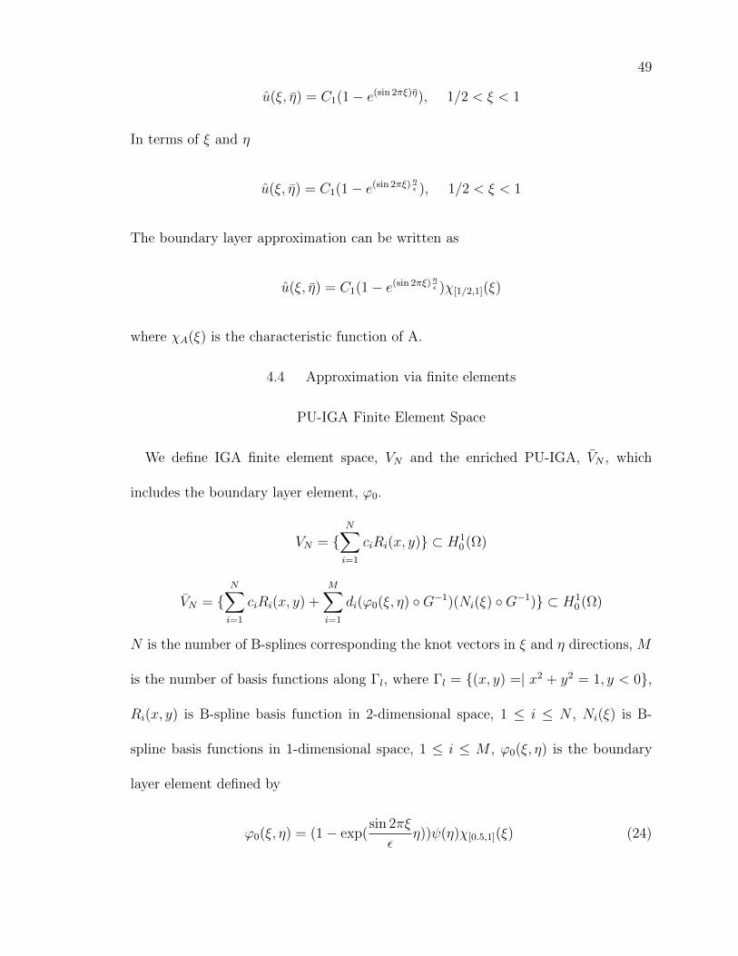
49

u(ξ, η) = C1(1− e(sin 2πξ)η), 1/2 < ξ < 1

In terms of ξ and η

u(ξ, η) = C1(1− e(sin 2πξ) ηε ), 1/2 < ξ < 1

The boundary layer approximation can be written as

u(ξ, η) = C1(1− e(sin 2πξ) ηε )χ[1/2,1](ξ)

where χA(ξ) is the characteristic function of A.

4.4 Approximation via finite elements

PU-IGA Finite Element Space

We define IGA finite element space, VN and the enriched PU-IGA, VN , which

includes the boundary layer element, ϕ0.

VN = N∑i=1

ciRi(x, y) ⊂ H10 (Ω)

VN = N∑i=1

ciRi(x, y) +M∑i=1

di(ϕ0(ξ, η) G−1)(Ni(ξ) G−1) ⊂ H10 (Ω)

N is the number of B-splines corresponding the knot vectors in ξ and η directions, M

is the number of basis functions along Γl, where Γl = (x, y) =| x2 + y2 = 1, y < 0,

Ri(x, y) is B-spline basis function in 2-dimensional space, 1 ≤ i ≤ N , Ni(ξ) is B-

spline basis functions in 1-dimensional space, 1 ≤ i ≤ M , ϕ0(ξ, η) is the boundary

layer element defined by

ϕ0(ξ, η) = (1− exp(sin 2πξ

εη))ψ(η)χ[0.5,1](ξ) (24)

50

: boundary layer approximation multiplied by PU with flat-top, ψ(η) defined by

ψ(η) =

0, if η ∈ [b+ δ, 1]

φRg2(η−(b−δ)

2δ, if η ∈ [b− δ, b+ δ]

1, if η ∈ [0, b− δ]

We can now formulate the following discrete analogues of the problem (3.2) Find

uh ∈ VN and uh ∈ VN , respectively, such that

a(uh, v) = (f, v), ∀v ∈ VN

a(uh, v) = (f, v), ∀v ∈ VN

where a(·, ·) is as in (20).

4.5 Numerical Method

We present the results of numerical simulation of (1.1) using the general IGA

and the enriched PU-IGA, which is enriched by the boundary layer element through

boundary layer analysis.

We consider the finite element space VN spanned by

R1, R2, ..., RN

where N is the number of B-spline basis functions. To treat the boundary layers, we

add the boundary layer elements in VN . There are several ways to augment the basis

of VN by adding different boundary layer elements.

1. ϕ0(ξ1, η)N1(ξ), ϕ0(ξ2, η)N2(ξ), ..., ϕ0(ξM , η)NM(ξ)

51

2. ϕ0(0.75, η)N1(ξ), ϕ0(0.75, η)N2(ξ), ..., ϕ0(0.75, η)NM(ξ)

3. ϕ0(ξ, η)N1(ξ), ϕ0(ξ, η)N2(ξ), ..., ϕ0(ξ, η)NM(ξ)

where M is the number of B-splines in ξ direction on the lower semicircle. Here, ϕ0

is the boundary layer element defined in (24). First, we have M different enrichment

functions by plugging in different values in ξ direction. Second, we have only one

enrichment function by plugging in one value in ξ direction. In the first and second

one, we consider the boundary layer element as a function of η. Lastly, we have a

boundary layer element as a function of ξ and η. For our implementation, we are

going to use the second choice of boundary layer element which is plugging a specific

value in ξ direction into the boundary layer element, namely,

ϕ0(η) = (1− exp(−ηε

))ψ(η)χ[0.5,1](ξ)

Incorporating the boundary layer elements that absorb the singularity behavior in

the finite space, we expect accurate numerical results in the PU-IGA setting. We

do not use costly mesh refinements near the boundary. We also prevent propagation

of the numerical errors along the characteristics inside of the domain Ω due to the

convective term in the problem, by using PU with flat-top.

Basis Functions

We have flexibility of how to design the basis functions. We might divide the

physical domain into several patches to apply different basis function in each patch.

See Figure 10. In the outer region (away from the boundary layer), we could obtain

optimal solution with general IGA. The boundary layer requires more sophisticated

52

basis function. That’s one of reason to divide the patches to increase the flexibility.

First, we only use one patch for the whole domain for simplicity. Next, we divide

the domain into two patches to enrich boundary layer only with boundary layer

approximation and use B-splines in regular zone.

Basis Functions on one patch

Let Ml(η) be the Berstein polynomials(special case of B-spline) of degree q defined

on [0, 1]

Ml(η) =

(q

l

)(1− η)q−lηl, l = 0, 1, 2, ..., q

Let Nk(ξ) be B-splines, corresponding to the open knot vector

0.....0︸ ︷︷ ︸p+1

, 1/4.....1/4︸ ︷︷ ︸p−1

, 1/2.....1/2︸ ︷︷ ︸p−1

, 3/4.....3/4︸ ︷︷ ︸p−1

1.....1︸ ︷︷ ︸p+1

The first and the last B-spline functions are joined together to be one basis function

so that the basis functions after push forward to the physical domain, can be periodic.

N1(ξ) =

(1− 4ξ)p, if ξ ∈ [0, 1/4]

0, if ξ ∈ [1/4, 3/4]

(4ξ − 3)p, if ξ ∈ [3/4, 1]

Namely,

N1(ξ) = N1(ξ) + N4p−2(ξ)

We define the periodic B-spline basis function in 2-dimensional on the parametric

domain as

Nk(ξ)Ml(η) | 1 ≤ k ≤ 4p− 3, 0 ≤ l ≤ q

53

Figure 9: Periodic basis function

Notice that we use 4p−3 of B-splines in ξ direction instead of 4p−2 of them to make

the B-splines periodic.

To prevent the influence of boundary layer element in outer region, we define the

boundary layer element multiplying the PU-function with flat-top, ψ(η).

ϕ0(η) = (1− exp(−ηε

))ψ(η)χ[0.5,1](ξ)

ψ(η) =

0, if η ∈ [b+ δ, 1]

φRg2(η−(b−δ)

2δ, if η ∈ [b− δ, b+ δ]

1, if η ∈ [0, b− δ]

Here, δ will be between 0.01 and 0.1 and 2δ is the width of non flat-top part of the

PU function. φRg2(x) = (1− x)2(1 + 2x) from (2.12).

We introduce the basis function enriched with boundary layer element as following

V := Nk(ξ)ϕ0(η)ψ(η) | 2p+1 ≤ k ≤ 4p−3⋃Nk(ξ)Ml(η) | 1 ≤ k ≤ 4p−3, 0 ≤ l ≤ q

54

Notice that we augment the boundary layer elements along the lower half circle for

k = 2p+ 1, ..., 4p− 3.

The inverse of the geometry mapping G defined in (3.3) is

G−1(x, y) = (ξ(x, y), η(x, y)) = (1

2πtan−1 y

x, 1−

√x2 + y2)

A family of enriched basis functions on the physical domain Ω is defined as V G−1.

Basis functions on two patches

Partition of the Domain

We consider a covering of the physical domain consisting of two patches: one disk

and one annular region shown in Fig. 10, that are defined as follows:

Ω∗1 = (x, y) : 0 ≤ x2 + y2 ≤ (1− (b− δ))2

Ω∗2 = (x, y) : (1− (b+ δ))2 ≤ x2 + y2 ≤ 1

To construct basis functions on these two patches, we need to construct PU functions

with flat-top, Ψ1,Ψ2, defined on two patches Ω∗1,Ω∗2, respectively. For this end, we

consider a covering of the parameter domain Ω consisting of the following two patches:

Ω∗1 = [0, 1]× [b− δ, 1] Ω∗2 = [0, 1]× [0, b+ δ].

55

Construction of PU function

We define PU functions Ψi, i = 1, 2, on rectangular patches Ω∗i , i = 1, 2, respectively,

as follows:

Ψ1(ξ, η) =

φLg2(

η−(b+δ)2δ

) if η ∈ [b− δ, b+ δ]

1 if η ∈ [b+ δ, 1]

0 if η /∈ [b− δ, 1],

Ψ3(ξ, η) =

φRg2(

η−(b−δ)2δ

) if η ∈ [b− δ, b+ δ]

1 if η ∈ [0, b− δ]

0 if η /∈ [0, b+ δ],

where φRg2(x) and φLg2(x) are C1-continuous functions defined by

φRg2(x) = (1− x)2(1 + 2x), and φLg2(x) = (1 + x)2(1− 2x).

Then we use the following parameters, PU functions, and patches.

1. Ω∗1 = G(Ω∗1), Ω∗2 = G(Ω∗2)

2. Ψ1(ξ, η) + Ψ2(ξ, η) = 1 for each (ξ, η) ∈ [0, 1]× [0, 1].

3. Let Ψk ≡ Ψk G−1, k = 1, 2 Then their supports are two patches defined by

(25): that is, supp(Ψk) = Ωk, k = 1, 2 shown in Fig. 10. In this figure, a narrow

annuls is non flat-top part of the PU functions Ψk.

4. We choose different parameters b, and δ for different diffusion coefficients ε: for

56

example,

b = 0.05(0.005), δ = 0.01(0.001) when ε = 10−3(10−4).

Ω∗1

Ω∗2

Figure 10: Diagram of supports of circular PU functions in the physical domain.

Ω∗1

Ω∗2

b− δb+ δ

1

0

Figure 11: Schematic diagram of patches in the reference domain. Ω∗1 = [0, 1]× [b−δ, 1], Ω∗2 = [0, 1]× [0, b+ δ].

57

Basis functions on Ω∗1

Let T1 : [b − δ, 1] −→ [0, 1] be the bijective linear mapping. This is η directional

Berstein polynomial transformed by T1.

MBk+1(η) = qCk(1− T2(η))q−kT2(η)k, k = 0, 1, 2, . . . , q (q ≥ 3).

Let Nk(ξ), k = 1, 2, . . . , 4p − 2, be B-splines, corresponding to an open knot vector

with p ≥ 3

0 . . . 0︸ ︷︷ ︸p+1

, 1/4 . . . 1/4︸ ︷︷ ︸p−1

, 1/2 . . . 1/2︸ ︷︷ ︸p−1

, 3/4 . . . 3/4︸ ︷︷ ︸p−1

, 1 · · · 1︸ ︷︷ ︸p+1

.

Next, N1 and N4p−2, the first and the last B-spline functions, respectively, are joined

together to be one blending function denoted by NB1 (ξ) so that they can be periodic

after push-forwarded to the innder disk Ω∗1 through the mapping G:

NB1 (ξ) =

(1− 4ξ)p if ξ ∈ [0, 1/4] (N1(ξ))

0 if ξ ∈ [1/4, 3/4]

(4ξ − 3)p if ξ ∈ [3/4, 1] (N4p−2(ξ))

NBk (ξ) = Nk(ξ), k = 2, . . . , 4p− 3

Now, the push-forward of the PU function Ψ1 of (25) onto the physical domain Ω

is denoted by

Ψ1(x, y) = (Ψ1 G−1)(x, y) = Ψ1(ξ(x, y), η(x, y)). (25)

58

Then basis functions on the annular region Ω∗1 are the following functions of class C0:

VA =

Ψ1(x, y) ·[(NBk × MB

l

)G−1

](x, y) : 1 ≤ k ≤ 4p− 3, 1 ≤ l ≤ q + 1

For the numerical methods for higher order equations, it is possible to modify the

members of VA to be C1 functions. Indeed, the basis functions in VA are C1 except at

points in (x, 0) : x ∈ (a−δ, b+δ), where(NBk ×MB

l

)G−1(x, y) have discontinuous

derivatives if k = 1. We can modify the joined B-spline (1− 4ξ)p and (4ξ− 3)p, to be

C1- continuous function into (1− 4ξ)p−1(1 + (p− 1)ξ) and (4ξ)p−1(p+ 1− 4pξ) .

Enriched basis functions on Ω∗2

Since the boundary layer occurs along the lower half of the unit circle, we enrich

this region with the boundary layer function (24).

Let T2 : [0, a + δ] −→ [0, 1] be the bijective linear mapping. This is η directional

Berstein polynomials transformed by T2.

MCk+1(η) = qCk(1− T3(η))q−kT2(η)k, k = 0, 1, 2, . . . , q,

NBk (ξ) are same periodic B-spline functions for Ω∗1 corresponding to the knot vector

(25). Then we have this augmented basis functions:

VB1 =NBk (ξ) · ϕ0(η) : k = 2p+ 1, . . . , 4p− 3

VB2 =

Ψ2(ξ, η) ·

(NBk (ξ) · MC

l (η))

: 1 ≤ k ≤ 4p− 3, 2 ≤ l ≤ q + 1

where Ψ2 is defined in (25).

Since MC1 (η) = 1 for η = 0 and the boundary layer problem has the homogeneous

59

boundary condition along ∂Ω, Ψ2(ξ, η) · NBk (ξ) · MC

1 (η) are excluded in VS2 .

We augment the enrichment function φ0(η) along the lower half circle for k =

2p+ 1, . . . , 4p− 3 in VS1 .

A family of enriched basis functions on the boundary layer region Ω∗2 is

VB =(VB1 G−1

)∪(VB2 G−1

). (26)

Then, combining these two sets VA,VB of basis functions constructed in previous

subsections, we have an approximation space V to deal with the boundary layer

effects.

V = span(VA ∪ VB

).

Note that V contains special boundary layer functions modified and scaled by PU

functions with flat-top.

Galerkin method

The finite element method for (3.1) is formulated as Galerkin’s method : Find uh ∈

VN such that

ε(∇u,∇v)− (uy, v) = (f, v), ∀v ∈ VN

where VN = ϕ1, ..., ϕN︸ ︷︷ ︸B-spline

, ϕN+1, ..., ϕN+M︸ ︷︷ ︸enriched

. Since

uh(x, y) =N+M∑i=1

ciϕi(x)

60

We can write

N+M∑i=1

ci[ε(∇ϕi,∇ϕj)− (∂ϕi∂y

, ϕj)] = (f, ϕj), j = 1, ..., N +M

In matrix form, the linear system (3.9) can be written as

Ac = b

where

A =

a11 . . . a1L

......

...

aL1 . . . aLL

, c =

c1

...

cL

, b =

b1

...

bL

where L=M+N, aij = ε(∇ϕi,∇ϕj)− (∂ϕi

∂y, ϕj), and bi = (f, ϕi). The stiffness matrix

consists of four block matrices, A1, A2, A3, A4,

A =

A1 A2

A3 A4

The submatrix A1 is composed of the terms involving only the B-splines whereas the

submatrices A2, A3 and A4 involve the boundary layer elements. For N + 1 ≤ i, j ≤

N +M , the bilinear form in A4 can be calculated as follows

a(∇ϕi,∇ϕj) = ε

∫∫Ω

∇ϕi∇ϕj −∂ϕi∂y

ϕjdxdy

=

∫∫Ω

(J(G)−1∇(Ni(ξ)ϕ0(η))T (J(G)−1∇(Nj(ξ)ϕ0(η))|J(G)|dξdη

−∫∫

Ω

(J(G)−12 ∇(Ni(ξ)ϕ0(η))(Nj(ξ)ϕ0(η))|J(G)|dξdη

61

where

J(G) =

∂x∂ξ ∂y∂ξ

∂x∂η

∂y∂η

=

−2π(1− η) sin 2πξ 2π(1− η) cos 2πη

− cos 2πξ − sin 2πξ

|J(G)| = 2π(1− η), determinant of Jacobian of G(ξ, η), geometry mapping. J(G)−1

2

is the second row of J(G)−1. For 1 ≤ i ≤ N,N + 1 ≤ j ≤ N + M , the bilinear form

in A2 can be calculated as follows

a(∇ϕi,∇ϕj) = ε

∫∫Ω

∇ϕi∇ϕj −∂ϕi∂y

ϕjdxdy

=

∫∫Ω

(J(G)−1∇(Ni(ξ)Mi(η)))T (J(G)−1∇(Nj(ξ)ϕ0(η))|J(G)|dξdη

−∫∫

Ω

(J(G)−12 ∇(Ni(ξ)Mi(η)))(Nj(ξ)ϕ0(η))|J(G)|dξdη

Numerical Simulation

Simulation 1

We consider 1-dimensional convection-diffusion problem.

ε4u+ (1 + ε)∇u+ u = 0, 0 < x < 1 (27)

u(0) = 0, u(1) = 1

Equation (27) can be solved exactly to get

u(x) =1

e−1 − e−1/ε(e−x − e−x/ε)

This u(x) is used to investigate the errors of the proposed schemes.

By the boundary layer analysis, we get the boundary layer approximation.

ui = C(1− e−x/ε), x = O(ε)

62

Table 3: 1D Perturbed Convection-Diffusion equation, Enriched PU-IGA and generalIGA Maximum error comparison, P- refinement, 4h = 0.1 ε = 0.001

Degree DOF NO Enrichment Enrichment

2 22 11843741332993504. 0.186389069746037084 42 1.8064901684905510 6.0128355627853125E-0096 62 1.1829919350432532 5.8175686490358203E-014

Introduce the boundary layer element ϕ0 as

ϕ0 = (1− e−x/ε)ψ1(x)

We compare the numerical results of general IGA and enriched PU-IGA by bound-

ary layer element. See the Figure 12 and Table 3 and 4. General IGA does not

yield reasonable solution to the problem from the table. One can find the oscillations

around boundary layer. With Enriched PU-IGA, we can have accurate solution and

can capture the boundary layer effect.

Figure 12: Comparison between general IGA and enriched PU-IGA, ε = 10−3, N =62,M = 1, 4h = 0.1, h-refinement

Simulation 2

Perturbed Convection-Diffustion Equation in a circle

63

Table 4: 1D Perturbed Convection-Diffusion equation, Enriched PU-IGA and generalIGA Maximum error comparison, H-refinement, p = 6, ε = 0.001

4h DOF NO Enrichment Enrichment

1 8 4.6265488088990887 0.691285472485981930.5 14 5.9244805022950153 0.353858550643678440.1 62 1.1829919350432532 5.8175686490358203E-014

Figure 13: Graphs of numerical solutions obtained by PU-IGA when ε = 10−3(Left)and ε = 10−5(Right).

We approximate the following exact solution u of (3.1)

u(x, y) =

(1− x2)2(−y +

√1− x2 + ε+

√1−x2

(1−x2)3/2), in Ω

0 on ∂Ω

The corresponding f can be found from (3.1) and it turns out that f = (1 − x2)2 +

O(ε). See [27]. With the derived the boundary layer element and basis functions, we

implement the enriched PU-IGA scheme and present the numerical result.

Relative error in percent in the l-norm ‖ · ‖l is defined by

‖err‖l,rel(%) =‖uex − uh‖l‖uex‖l

× 100.

64

Number of Degrees of Freedom

102

103

104

Rela

tive e

rrors

in L

2 n

orm

(%

)

10-1

100

101

102

103

PU-IGA with Adaptive Mesh

PU-IGA with Enrichment

IGA with Radical Mesh

Number of Degrees of Freedom

103

104

Rela

tive e

rrors

in L

2 n

orm

(%

)

10-2

10-1

100

101

102

103

PU-IGA with Adaptive Mesh

PU-IGA with Enrichment

IGA with Radical Mesh

Figure 14: (Left) Relative errors in percent when ε = 10−3, a− δ = 0.05, b = 0.5, δ =0.01. (Right) Relative errors in percent when ε = 10−4, a − δ = 0.005, b = 0.5, δ =0.001.

Results of the enriched PU-IGA using V as a approximation space are shown in

Fig. 13 and Fig. 14, and Table 5, in which we observe the following.

1. The proposed Enriched PU-IGA yields better results with lower degree of free-

dom than the enriched FEM of [27], as shown in Table 5. We compared our

results with those in Table 1 of [27].

2. The authors in [27] used piecewise linear basis functions for enriched FEM,

whereas we use high order B-spline basis functions constructed through either

the p-refinement or the k-refinement . Thus, Enriched PU-IGA requires more

quadrature points than the enriched FEM of [27] for numerical integration. If

no internal knots are repeated in the k-refinement of IGA, the support of a B-

spline function of degree p covers p+ 1 (non-void) knot spans for extreme cases

65

Hence, the integral domain of a B-spline function of degree p can be divided

into p + 1 intervals for accurate integrations. Therefore, we cannot claim that

the total computing time of our method is shorter than that of the enriched

FEM used in [27].

For the results in Table 5, we use the p-refinement of IGA in which internal

knots are repeated (p− 1) times and hence supports of corresponding B-splines

consist of two knot spans. For a comparison of computing time between PU-

FEM and PU-IGA, suppose each piecewise linear basis function consists of four

2-dimensional shape functions in FEM. We use B-splines of degrees p = 10 and

q = 10 in the framework of the p-refinement of IGA. Then we may use one

Gauss point per shape function in FEM, whereas we use six Gauss points per

B-spline function of degree 10 on each knot span. Thus we have the following.

• The number of function evaluations is 9217×4 = 36, 868 in FEM, whereas

the number of function evaluations is 3692× 36× 4 = 531, 468 in the pro-

posed method. Here 9217 and 3692, respectively, are degrees of freedom

shown at the last row of Table 5. That is, since the polynomials of degree

10 have more terms than linear polynomials, the proposed method requires

much more function evaluations than Enriched FEM for numerical integra-

tions. Since both enriched IGA and enriched FEM use a similar boundary

layer function as an enrichment, extra Gauss points used for evaluations

of enrichment functions and PU functions are not counted.

By the same reasons, if we assume that the bandwidths k of IGA and FEM are

66

similar (refer to [60] for detailed discussion of bandwidth), then we have the

following.

• The Cholesky factorization costs 9217(k2 + 3k) flops for the enriched PU-

FEM and 3692(k2 + 3k) flops for the enriched PU-IGA, respectively. That

is, the enriched PU-FEM requires more flops for the factorization than the

proposed method.

3. In both cases where ε = 10−3 as well as ε = 10−4, PU-IGA yields numerical

solutions with relative error 0.00038, which is as small as ε. Since we com-

pare PU-IGA solutions with approximate true solution that satisfies the stiff

convection-diffusion equation only upto ε, it has no meaning to pursue more

accurate solutions than those in the column “enriched PU-IGA” and “ PU-IGA

adaptive” of Table 5.

4. PU-IGA with adaptive k-refinement and Enriched PU-IGA by the boundary

layer function are compared as follows:

• We use B-splines of high order (6 ≤ p ≤ 12) as basis functions for both

approaches. As shown in Table 5, the enriched PU-IGA yields accurate

solution at low cost (dof = 2784).

• For PU-IGA with adaptive mesh shown in Fig. 14, we choose Ω∗3 to be

almost as small as the boundary layer zone and insert knots adaptively

for the k-refinement of the radial direction basis MCl (η), 1 ≤ l ≤ q + 1. In

other words, using the PU function Ψ2, basis functions of high degree are

67

enriched PU-IGA PU-IGA adapt msh Hong et al.[27] IGA with radical mshdof ‖err‖L2,rel(%) dof ‖err‖L2,rel(%) dof ‖err‖L2,rel(%) dof ‖err‖L2,rel(%)

1352 69.56 1332 70.01 1516 5.77 400 4.0672004 3.480 1980 3.516 2347 5.01 1024 1.0312784 0.074 2756 0.113 4130 4.43 1936 0.9293692 0.038 3660 0.041 9217 3.39 3136 0.929

Table 5: Relative error in percent when ε = 10−4. The results in the third columnare relative errors in percent by enriched FEM reported in [27].

constructed inside the boundary layer zone. Relative errors in the last row

of the column “ PU-IGA Adapt msh” of Table 5 show that PU-IGA with

adaptive mesh is as good as Enriched PU-IGA enriched with boundary

layer function.

Ω1 Ω2

a− δ a+ δ

(1, 1)

(1, 0)

Figure 15: Schematic diagram of subdomains in the reference domain. Ω1 = [0, a]×[0, 1], Ω2 = [a, 1] × [0, 1], where a = 0.1 and δ = 0.05. The supports of PU functionswith flat-top, Ψ1 and Ψ2, are Ω∗1 = [0, a+ δ]× [0, 1] = supp(Ψ1), and Ω∗2 = [a− δ, 1]×[0, 1] = supp(Ψ2).

Simulation 3

Perturbed Convection-Diffustion Equation in a square

To present the effectiveness of the proposed enriched PU-IGA, we compare the

68

performance of enriched PU-IGA with other numerical methods. For a simplicity, we

test it with a singularly perturbed convection-diffusion problem with mild boundary

layer effect.

Let us consider a singularly perturbed convection-diffusion problem with an expo-

nential layer at the outflow boundary and two characteristic layers. A problem like

this is given by

−ε∆u− bux + cu = f in Ω = (0, 1)2, (28)

u = 0 on ∂Ω

where b = 2 − x, c = 3/2, ε = 10−2, and f is calculated from the following solution

of (28)

u(x, y) =

(cos

πx

2− e−x/ε − e−1/ε

1− e−1/ε

)(1− e−y/

√ε)(1− e−(1−y)/

√ε)

1− e−1/√ε

The function has an exponential boundary layer at x = 0, two characteristic boundary

layers at y = 0 and y = 1, respectively.

To find the inner approximation, we introduce a boundary-layer coordinate given

as

x =x

εα

When using this boundary-layer coordinate, (28) transforms to

−ε1−2α∂2u

∂x2− ε∂

2u

∂y2− 2ε−α

∂u

∂x+ x

∂u

∂x+ 2/3u(εαx, y) = f(εαx, y)

69

The boundary condition is

u(0, y) = 0

The leading terms are

−ε1−2α∂2u

∂x2, −2ε−α

∂u

∂x= 0

By the dominant balancing, α = 1. With this we have the following problem to solve:

−∂2u

∂x2+ 2

∂u

∂x= 0

The general solution of this problem is

ui(x, y) = C(1− e−2xε )

where C is a constant that we could find by matching condition. We use use ϕ0(x)

as

ϕ0(x) = 1− e−2xε

In this simulation, the parameter domain and the physical domain are both [0, 1]×

[0, 1] and the geometric mapping G is the indentity mapping. For the results in Table

6 and Fig. 16, we use the following parameters and PU-functions:

We divide the reference domain, Ω = [0, 1] × [0, 1] into two subdomains shown in

the Fig. 15:

Ω1 = [0, a]× [0, 1], Ω2 = [a, 1]× [0, 1], where a = 0.1.

Two PU-function with flat-top are defined by

Ψ1(ξ, η) = ψ(δ,1)[0,a] (ξ)× η and Ψ2(ξ, η) = ψ

(δ,1)[a,1] (ξ)× η,

70

where δ = 0.05. Then the supports of Ψ1 and Ψ2, respectively, are [0, a + δ] ×

[0, 1] and [a− δ, 1]× [0, 1].

The refinements, B-splines, and an enrichment function used to get the results in

Fig. 16 are as follows:

1. For the result of “ PU-IGA ”, we use two different sets of basis functions in the

ξ-direction:

(i) the scaled B-splines N[0,a+δ]k,p+1 (ξ) · ψ(δ,1)

[0,a] (ξ), k = 1, . . . , n1 that are B-spline

functions corresponding to an open knot vector on [0, a + δ], scaled by the PU

function ψ(δ,1)[0,a] (ξ).

(ii) the scaled B-splines N[a−δ,1]l,p+1 (ξ) · ψ(δ,1)

[a,1] (ξ), l = 1, . . . , n2, that are another set

of B-splines corresponding to an open knot vector on [a − δ, 1], scaled by the

PU function ψ(δ,1)[a,1] (ξ).

2. For the result of “ Enriched PU-IGA ” of Table 6 and Fig. 16, we use the

following basis functions:

(i) By the boundary layer analysis, we get φ0(ξ) = 1−e−2ξ/ε . On the boundary

layer zone [0, a+ δ]× [0, 1], we use the enrichment functions Hj(ξ, η) defined by

Hj(ξ, η) =(φ0(ξ) · ψ(δ,1)

[0,a] (ξ))×Mj(η), 0 ≤ j ≤ p,

as well as

(N

[0,a+δ]k,p+1 (ξ) · ψ(δ,1)

[0,a] (ξ))×Mj(η), 2 ≤ k ≤ n1, 0 ≤ j ≤ p,

where Mj(η), j = 0, 1, . . . , p, are Bezier functions of degree p.

71

Because of the enrichment function φ(ξ), it is not necessary to use B-splines

corresponding to a fine mesh on the boundary layer zone.

(ii) On [a − δ, 1], we construct B-splines by the k-refinement of IGA in the ξ-

direction. For example, the set of Bezier polynomials, defined on [a − δ, 1], of

degree p is refined by inserting equally spaced p knots and scaled by the PU

function ψ(δ,1)[a,1] (ξ).

3. For the result of ”IGA with radical mesh refinement”, we use B-splines obtained

by the k-refinement by inserting nξ knots:

ri =( i

nξ + 1

)1/3, i = 1, . . . , nξ,

where the number of knots, nξ, is increased as the p-degree is elevated.

4. For the result of “ IGA ”, we use the k-refinement of IGA in both ξ- and

η-directions.

Even though the boundary layer effect is not very strong (since ε = 10−2 ), from

the results shown in Table 6 and Fig. 16, we observe the following:

1. Enriched PU-IGA is superior over any other methods (including streamline

diffusion techniques).

2. One can use only one patch with sufficiently large number of knot insertions in

the k-refinement of IGA to get similar results to enriched PU-IGA. However, in

such case, the degrees of freedom become much lager.

72

Number of Degrees of Freedom

101

102

103

Re

lative

err

ors

(%

) in

L2 n

orm

10-8

10-6

10-4

10-2

100

102

IGA

IGA with Radical Mesh

PU-IGA

PU-IGA with Enrichment

Figure 16: Relative errors in L2-norm in percent from results obtained by IGA, PU-IGA, Enriched PU-IGA, and IGA with radical mesh.

IGA PU-IGA Enrich PU-IGA IGA with Rad mshdof(p-deg) ‖err‖L2,r(%) dof ‖err‖L2,r(%) dof(p-deg) ‖err‖L2,r(%) dof ‖err‖L2,r(%)

121(6) 8.98E-0 119 2.32E-2 65(4) 4.39E-1 121 1.13E-0225(8) 1.52E-0 180 1.02E-2 107(6) 7.47E-2 225 9.93E-2

361(10) 1.35E-1 275 1.38E-3 195 (8) 3.81E-3 361 5.07E-3529(12) 7.84E-3 364 3.10E-4 309 (10) 1.80E-4 529 3.60E-4729(14) 3.12E-3 495 3.08E-5 449 (12) 7.59E-6 729 9.50E-5

612 2.08E-6 615 (14) 6.14E-7

Table 6: Relative errors in L2-norm in percent of numerical solutions obtained byIGA, PU-IGA, Enriched IGA, and IGA with radical mesh refinement when ε = 10−2.

73

Figure 17: Ellipse Geometry Mapping

4.6 Singulary perturbed convection-diffusion equation on an ellipse domain

We consider the same convection-diffusion problem on a different domain, an ellipse

domain. −ε4u− uy = f(x, y) in Ω

u = 0 on ∂Ω

where 0 < ε 1, Ω is an ellipse centered at (0, 0) and one radius along the x-axis is

2r and the other along the y-axis is r.The function f is as smooth as needed.

The geometry mapping G : Ω −→ Ω is defined by

G(ξ, η) = (x(ξ, η), y(ξ, η) = (2(1− η) cos 2πξ, (1− η) sin 2πξ)

where η = 1− r, r is the distance to the origin along the y-axis and 2πξ is the polar

angle from origin of the ellipse. We define the reference domain Ω = [0, 1]× [0, 1] and

divide the domain into two patches, Ω1 = [0, 1]× [0, b+ δ] and Ω2 = [0, 1]× [b− δ, 1].

See Figure 17.

To find the boundary layer element, we pullback the problem (5.1) on to the refer-

ence space. Using the stretched variable, η = ηεα

. we obtain the transformed equation

74

of (5.1).

3ε

4π(1− εαηsin 2πξ cos 2πξ

∂u

∂ξ− ε

4π2(1− εαη2(1

4sin2 2πξ + cos2 2πξ)

∂2u

∂ξ2

+ε1−α

1− εαη(1

4sin2 2πξ + cos2 2πξ)

∂u

∂η+

ε1−α

2π(1− εαη)sin 2πξ cos 2πξ

∂2u

∂η∂ξ

−ε1−2α(1

4sin2 2πξ + cos2 2πξ)

∂2u

∂η2− 1

2π(1− εαη)cos 2πξ

∂u

∂ξ+ ε−α sin 2πξ

∂u

∂η= f

Dominating terms are

−ε1−2α(1

4sin2 2πξ + cos2 2πξ)

∂2u

∂η2, ε−α sin 2πξ

∂u

∂η

Therefore a consistent scaling is possible if we select α = 1. Because we are interested

only in the leading-order approximation, we obtain

−(1

4sin2 2πξ + cos2 2πξ)

∂2u

∂η2+ sin 2πξ

∂u

∂η= 0

The general solution is

ui = C1 + C2esin 2πξ

1/4 cos2 2πξ+sin2 2πξη, 1/2 < ξ < 1

Because the boundary layer is located near η = 0, we apply the boundary condition

u = 0 at η = 0, and so

ui = C1(1− esin 2πξ

1/4 cos2 2πξ+sin2 2πξ

ηε ), 1/2 < ξ < 1

We modify the boundary layer approximation to get our boundary layer element.

Choose ξ = 3/2 for numerical simulation and we can get the boundary layer element

ϕ0 = 1− e−ηε

75

With proposed Enriched PU-IGA, we expect to get an accurate solution on ellipse

domain too.

CHAPTER 5: SINGULARLY PERTURBED PARABOLIC EQUATION IN ACIRCLE

5.1 Introduction

We consider the two-dimensional singularly perturbed heat equation of the form

∂u∂t− ε4u = f, in Ω× (0, T )

u(x, y, t) = 0, on ∂Ω× (0, T )

u(x, y, 0) = u0(x, y), on Ω

(29)

where 0 < ε 1 is the heat conductivity and Ω is the unit circle centered at (0,

0). The functions f and u0 are assumed to be sufficiently regular. We also assume

the compatibility condition

u0 = 0 on ∂Ω

The numerical methods for singularly perturbed problems have been studied in

many articles. [58], [59], [63] and [64] proposed numerical methods for stationary

convection-diffusion equations using finite element methods. One can find numerical

results for parabolic type problems in [9], [12], [33], [39] and [69]. In those articles

the authors utilized mesh refinement near the boundary layer. Furthermore, for the

parabolic type cases, the authors mainly focused on the finite difference methods in a

unit interval or rectangular domains and this did not address the issue of the curved

boundary in the context of time dependent problems. In [29], the author approxi-

77

mates problem (29) using a quasi-uniform triangulation and P1 finite element space

enriched with boundary layer correctors constructed near the circular boundary. In

this paper, we similarly aim to approximate problem (29) using B-spline based Isogeo-

metric Finite Element space enriched with boundary layer approximation constructed

near the boundary layer. We avoid the costly mesh refinements at the boundary by

enriching the Finite Element Space. Boundary layer element multiplied by Partition

of Unity with flat-top does not affect out of boundary layer zone.

We introduce the boundary layer element based on the boundary layer analysis sim-

ilar to that of [29]. Incorporating the boundary layer element, we obtain the proposed

NURBS based enriched Finite Element space to be used in the numerical simulations

with the coarsest mesh. We present the results of our numerical simulations using

B-spline based PU-IGA Finite Element method with the enrichment element.

For the time-dependent problems, the mesh refinement is costly since we need to

solve the linear system at each time step. Avoiding mesh refinement, [29] approached

the problem in classical Finite Element setting. In this paper, we solve the problem

similarly in Enriched PU-IGA setting without mesh refinement. We believe this

Enriched PU-IGA used in this paper should also be applicable to many other types of

time-dependent singularly perturbed problems such as reaction-diffusion equations.

The concept of enriched space and boundary layer element was first introduced in

[26]. The authors of [5] and[6] introduced independently a similar concept for the

one-dimensional equations. Especially in [6], the authors studied the numerical anal-

ysis of the one-dimensional time-dependent problem. In [16, 18], and [19] the authors

presented the numerical methods for the two-dimensional stationary convection dif-

78

fusion equations using the finite element methods and finite volume methods in a

rectangular domain. Lately, in [12, 14] and [20], the time-independent equations were

considered in a circular domain.

5.2 Discretization

The semi-discrete analogue of (29) will be based on the variational formulation :

Find u(t) ∈ V , t ∈ I such that

(u(t), v) + a(u(t), v) = (f(t), v) ∀v ∈ V, t ∈ I (30)

u(0) = u0

Now, let Vh be a finite-dimensional subspace of V with basis ϕ1, ϕ2, ..., ϕN , ϕN+1, ..., ϕN+M.

We get the following semi-discrete analogue of (30): Find uh(t) ∈ Vh, t ∈ I, such

that

(uh(t), v) + a(un(t), v) = (f(t), v) ∀v ∈ Vh, t ∈ I (31)

(uh(0), v) = (u0, v) ∈ Vh

In the classical backward Euler method for the semi-discrete problem (31) we seek

approximations uhn ∈ Vh of u(., tn), n = 0, ..., N , satisfying

(unh − un−1

h

kn, v) + a(unh, v) = (f(tn), v) ∀v ∈ Vh, n = 1, 2, , .., N (32)

(u0h, v) = (u0, v) ∀v ∈ Vh

The classcial time-discretization method, the backward Euler method satisfies sta-

bility condition so is stable regardless of the size of the time steps kn, namely this

79

method is unconditionally stable.

5.3 Boundary Layer Analysis

The formal limit problem(unperturbed problem) of (29), namely when ε −→ 0, is∂u∂t

= f, in Ω× (0, T )

u(x, y, 0) = u0(x, y) on Ω

(33)

We find the explicit solution

uouter(x, y, t) = u0(x, y) +

∫ t

0

f(x, y, s)ds

Define a geometry Mapping G : [0, 1]× [0, 1] −→ Ω by

G(x, y) = ((1− η) cos 2πξ, (1− η) sin 2πξ)

To investigate the boundary layer in the circular domain, we pull back the (29) on to

the parameter space by the geometry mapping, G. Using the change of variables, we

obtain

∂u

∂x= − sin 2πξ

2π(1− η)

∂u

∂ξ− cos 2πξ

∂u

∂η

∂u

∂y= − cos 2πξ

2π(1− η)

∂u

∂ξ− sin 2πξ

∂u

∂η

4u =∂2u

∂x2+∂2u

∂y2

=∂2u

∂η2− 1

1− η∂u

∂η+

1

(1− η)2

∂2u

∂ξ2

80

(29) becomes

∂u

∂t− ε4u =

∂u

∂t− ε∂

2u

∂η2− ε

4π2(1− η)2

∂2u

∂ξ2+

ε

1− η∂u

∂η= f(G(ξ, η))

We look for the expansion of u at fist order:

u ' uouter + uinner

where uouter is the solution of (33) and uinner is the first order boundary layer ap-

proximation. Setting f = 0 in (29), we introduce the stretched variable to find the

boundary layer approximation.

η =η

εα

(4.1) is transformed to

∂u

∂t− ε1−2α∂

2u

∂η2− ε

4π2(1− εαη)2

∂2u

∂ξ2+

ε1−α

1− εαη∂u

∂η= 0

The coefficients of the terms in the differential equation are

1, ε1−2α, ε, ε1−α

To determine α, we estimate these magnitudes by dominant balancing. The domi-

nating terms are

∂u

∂t− ε1−2α∂

2u

∂η2= 0

A consistent scaling is possible if we select α = 12. Thus, the reasonable thickness of

the boundary layer is α = 12. We obtain the equations for boundary layer approxi-

81

mation:

∂u∂t− ∂2u

∂η2= 0, in Ω× (0, T )

u(0, t) = −uouter at η = 0

u(x, 0) = 0

u −→ 0, as η −→∞

(34)

See [29]. The solution of (34) is

ui = −∫ t

0

I(η, t− s)∂uouter∂t

(ξ, 0, s)ds

where

I(x, t) = erfc(x√2εt

)

erfc(z) = 1− erf(z) =

√2

π

∫ ∞z

exp(−y2

2)dy

erf(z) =

√2

π

∫ z

0

exp(−y2

2)dy

See [10]

5.4 Error Estimates for fully discrete approximations

This is an error estimate for the backward Euler scheme with Vh piecewise linear

from [32]

Theorem Let Un be the numerical solution of (32) and u is the solution of (29) for

n = 1, ..., N , then there is a constant C such that

‖u(tn)− Un‖ ≤ C(1 + log(tnkn

)1/2)(maxm≤n

∫Im

‖u(s)‖ds+ maxt≤n

h2‖u(t)‖H2(Ω)) (35)

82

Absorbing the almost bounded logarithmic quantity in the constant C, and using the

trivial fact that ∫In

‖u(s)‖ds ≤ kn‖u‖∞,In

where ‖v‖∞,J = sups∈J ‖v(s)‖ We can write (35) alternatively as follows

maxt∈I‖u(t)− U(t)‖ ≤ C(max

n≤Nkn‖u‖∞,In + max

t∈Ih2‖u(t)‖H2(Ω)) (36)

5.5 Numerical Simulations

We present the results of numerical simulations of (29) using the general IGA and

Enriched PU-IGA.

Modified Boundary Layer Element

We do not use the boundary layer approximation directly since the term I(η, t −

s) is not convenient for the integration. Instead, We modify the boundary layer

approximation for numerical simulation.

uinner ∼∫ t

0

I(x, t− s)ds, f is bounded

=

∫ t

0

1− 1√πεt

e−x2

4εtds

∼ 1− 1√πεt

e−x2

4εt , t is bounded

We simply the boundary layer element ϕ0 for numerical simulation:

ϕ0(x, t) = (1− e−x2

4εt )ψ1(x)

83

where ψ1(x) is PU with flat-top which makes the boundary layer element not affect

the outer zone.

Simulation 1: One-Dimensional Example

We present a simple one-dimensional example To compare the numerical solution

with the exact solution, we consider the following equations:

ut − εuxx = f(x, t), (0, 1)× (0, T )

u(0, t) = u(1, t) = 0, t ∈ (0, T )

u(x, 0) = u0(x), x ∈ (0, 1)

We choose the exact solution u as

u = t(1− e−x√ε cos(

x√ε))(1− cos(

1− x√ε

)e− 1−x√

ε )

Hence, f is computed from the (29).

We have two boundary layers at each boundary. Similarly, we could derive the

boundary layer element at x = 1. Since φ0 depends on time, for each time step,

we need to calculate different boundary layer element. To improve computational

efficiency, we introduce the modified time-independent boundary layer elements φ0

and φ1 such that

φ0(x) = 1− exp(−x2

4ε)ψ1(x) (37)

φ1(x) = 1− exp(−(1− x)2

4ε)ψ3(x) (38)

where ψ1 and ψ3 partition unity functions are used to avoid the singularity of φ at

84

Table 7: Enriched PU-IGA and IGA Maximum errors, H- refinement, p = 12

4h DOF No Enrichment Enrichment

1 13 0.60845711245515210 2.0256926718709600E-0020.5 25 0.35453147267928342 6.8586187221852946E-0030.1 121 2.0443482651402722E-002 6.4348526507274073E-013

x = 0 and x = 1.

ψ1(η) =

0, if η ∈ [a+ δ, 1]

φRg2(η−(a−δ)

2δ, if η ∈ [a− δ, a+ δ]

1, if η ∈ [0, a− δ]

ψ3(η) =

0, if η ∈ [0, b− δ]

φLg2(η−(b+δ)

2δ, if η ∈ [b− δ, b+ δ]

1, if η ∈ [b+ δ, 1]

where φRg2(x) = (1− x)2(1 + 2x)

φLg2(x) = (1 + x)2(1− 2x)

We present the results of numerical simulation of (29) using the general IGA and

Enriched PU-IGA, which is enriched by the boundary layer element by boundary layer

analysis. In Figures 18 and 19, we observe that general IGA produce oscillations near

the boundary, however, with Enriched PU-IGA the boundary layer elements capture

the sharp transition near the boundary. According to Tables 7 and 8, we observe that

the errors of Enriched PU-IGA is much smaller than that of general IGA.

85

Figure 18: Comparison between IGA and Enriched PU-IGA, ε = 10−5, N = 25,M =2, 4h = 0.5, h-refinement

Figure 19: comparison between IGA and Enriched PU-IGA, ε = 10−5, N = 121,M =2, 4h = 0.1, h-refinement

1D Error estimates for IGA

Consider this problem for error estimate

u = e−xt(1− e−x√ε cos(

x√ε))(1− cos(

1− x√ε

)e− 1−x√

ε )

We use the boundary layer elements (37) developed in the last section. We calculate

the convergence rate for h and k, by

log ei+1

ei

log ti+1

ti

86

Table 8: Enriched PU-IGA and IGA Maximum errors, K- refinement, p = 12

4h DOF No Enrichment Enrichment

1 15 0.60845711245515210 2.0256926718709600E-0020.1 24 0.12410087048350116 8.6750421698587044E-0030.01 114 1.3111940128840427E-004 6.2950588269217178E-005

Table 9: H-refinement in space direction, Error and convergence rate with p = 1,4k = 0.001

4h DOF Error Convergence Rate

1 2 0.86719158608753943 0.565776486022907420.5 3 0.58586743917746709 1.27342342292684240.1 11 7.5459621590306891E-002 1.97397473085385620.05 21 1.9208304413022126E-002 1.98259947601550630.01 101 7.9015350227129577E-004 1.96090852093720520.005 201 2.0296407621556156E-004

where ei is error at the time level ti.

The numerical results show that the space convergence rate is about 2 and time

convergence rate is about 1. See the Table 9 and 10. The results support the Theorem

35.

Table 10: H-refinement in time direction, Error and convergence rate with p = 1,4h = 0.01

4k DOF Error Convergence rate

1 101 0.15387596258839775 0.846591736152186300.5 101 8.5569946676072428E-002 0.939839187324702730.1 101 1.8853928667987407E-002 0.978720589356580020.05 101 9.5670403064213039E-003 0.983696936165317390.01 101 1.9642777850752413E-003 0.968731751003142680.005 101 1.0036576763091665E-003

CHAPTER 6: FOURTH ORDER ELLIPTIC EQUATIONS CONTAININGSINGULARITIES

6.1 Introduction

We consider the two-dimensional 4th order equations on cracked disk.

42u = f in Ω

u(1, θ) = ∂u∂n

(1, θ) = 0 on ∂Ω

u(r, 0) = u(r, 2π) = 0

∂u∂y

(r, 0) = ∂u∂y

(r, 2π) = 0

where Ω is the cracked unit disc centered at (0, 0). The equation satisfy clamped

boundary conditions.

The numerical approximation of high order Partial Differential Equations(PDEs)

represents a challenging task for the classical Galerkin Finite Element methods due

to the need to use trail and test functions featuring high degree of continuity. This

issue has been addressed by adapting existing Finite Element schemes or developing

new numerical schemes. Specifically, the Discontinuous Galerkin(DG) [57] and local

Discontinuous Galerkin(LDG) methods in [15] were developed and adapted for solv-

ing high order PDEs. Analogously, non-conforming discretizations have been used

to achieve the needed global regularity [11]. Ad hoc techniques as continuous dis-

continuous finite element approximations for fourth order PDEs have been developed

88

in [19] in order to overcome the issue of defining C1-continuous basis for arbitrary

shaped elements in dimensions greater than one. Currently, the golden standard in

the framework of the standard Galerkin method with Lagrangian basis functions,

consists in resorting to mixed formulations [20]. Spectral or pseudo-spectral domain

decomposition techinigues have also been used to approximate fourth order PDEs

[54]. Isogeometric Analysis(IGA) is a recently developed computational methodology

in [16] aiming at closing the existing gap between Computed Aided Design (CAD)

and Finite Element Analysis (FEA). Based on the isogeometric paradigm, for which

the same basis functions used to present the known geometry are then used to ap-

proximate the unknown solution of the PDEs, IGA has been successfully used for the

numerical approximation of a wide range of problems providing accurate and efficient

solutions. Moreover, IGA provides advantages in the numerical approximation of high

order PDEs within the framework of the standard Galerkin formulation, since in IGA

globally smooth basis functions can be eventually used. Besides the possibility of

offering simplified refinements procedures, IGA allow to exactly represent geometries

in engineering design.

However, NURBS or B-spline functions do not satisfy the boundary conditions for

the fourth order differential equations. Also the standard refinements of IGA do not

yield reasonable solutions to fourth-order equations containing singularities.

In this work, B-splines are modified minimally to satisfy the given boundary con-

ditions using Partition of Unity with flat-top. To handle singularities on the cracked

domain, the modified B-spline functions are enriched by singular functions that re-

semble the singularities of the fourth-order equation.

89

However, these kind of enrichment methods (GFEM or X-FEM) have to deal with

large condition numbers of stiffness matrix and integrals of singular functions. In

other words, the Galerkin method in the framework IGA have a stiffness matrix with

large condition number and standard quadrature rules does not give accurate integrals

of derivatives of enrichment functions.

In this work, we propose a mapping method that overcome these drawbacks of

enriched IGA. This proposed mapping method has same result as the enrichment

methods with minimal condition number and without singular integrals. The map-

ping method is developed for one-dimensional problem and is extended to the second-

dimensional fourth-order equations on a cracked disk. In the frame of FEM, a map-

ping method for the elasticity equations on cracked domain, was introduced in [42].

Also, in the frame of IGA, a mapping method for second order PDEs with singulari-

ties was introduced [48]. We generalize the proposed mapping method introduced in

[48] and apply it to fourth-order equation containing singularities.

The outline of this chapter is as follows. In section 2, we present mapping method

scheme for one-dimensional problem and test this approach to fourth-order equation

with singularity. In section 3, This mapping method scheme is developed and tested

for second dimensional problems on cracked domain. Conclusions follow.

90

6.2 Enriched PU-IGA and PU-IGA with Mapping Method

Consider the following model problem with clamped boundary conditionsu(4)(x) = f(x) in (a, b)

u(a) = u′(a) = 0

u(b) = u′(b) = 0

(39)

Let V = w ∈ H2(a, b) : w,w′ ∈ H10 (a, b)be the function space. Multiplying the

equation by an arbitrary function v ∈ V and integrating over the interval, we have

∫ b

a

u(4)vdx =

∫ b

a

u(2)v(2)dx =

∫ b

a

fvdx ∀v ∈ V

Thus the variational equation is

B(u, v) ≡∫ b

a

u(2)v(2)dx =

∫ b

a

fvdx ≡ F(v), ∀v ∈ V

We construct an example of a fourth-order equation containing singularity of the

type xα. To determine how strong the intensity of singularity α is allowed, we prove

the following lemma.

Lemma 2. Suppose v ∈ H20 (a, b), 0 ≤ a < b. Then

(1) |v(x)| < Cx1.5 (40)

(2) |∫ b

a

xα−4v(x)dx| <∞ if α > 1.5. (41)

Proof. (1)

Since v(x) ∈ H20 (a, b), v′(x) ∈ H1

0 (a, b),

then |v′(x)| < Cx0.5, C ∈ R by Theorem 7.17 in [21]

91

Hence we have

|v(x)| = |∫ x

a

v′(t)dt| ≤ C

∫ x

0

t0.5dt ≤ Cx1.5.

(2) ∣∣∣ ∫ b

a

xα−4v(x)dx∣∣∣ ≤ C

∫ b

0

xα−4x1.5dx

For this to be integrable, α− 4 + 1.5 > −1

Therefore, α > 1.5

We use the Enriched PU-IGA which is developed for the singularly perturbed prob-

lems, to solve the fourth-order equation with singularities. In singularly perturbed

problems, we do not know the boundary layer functions so that we approximate the

boundary layer functions and use the approximation as enrichment function. We

approximate the boundary layer function on the reference domain not on physical

domain. We add the boundary layer approximation and push-forward them to the

physical domain to construct the Finite Element Space.

Here, we consider the problem whose singular solution is already known, like crack

singularities. We propose two ways to solve the fourth-order equations containing

singularities. First, we add singular functions into the Finite Element Space directly.

We call this Enriched PU-IGA. Secondly, to get the singular function on the physi-

cal domain, we construct a particular Mapping from the reference domain onto the

physical domain to generate singular functions on the physical domain. We call this

approach PU-IGA with Mapping Method.

The k-refinement, the p-refinement, the reduced p-refinement of IGA for Enriched

PU-IGA. Since the fourth-order derivative of singular functions are highly singular, a

92

special treatment, substitution method are needed for integrals of singular functions.

Enriched PU-IGA gives accurate solution, but yields large condition numbers.

In PU-IGA with Mapping Method, the singular functions are generated through a

particular mapping. Hence this method does not have a large condition number nor

integrals of singular functions.

Enriched PU-IGA

We present the detail scheme of enriched PU-IGA for fourth-order equation with

singularities. For simplicity, we assume that the physical domain is the same as

the reference domain. Therefore, B-spline functions Ni,p+1(ξ) and its push-forward

Ni,p+1(x) onto the physical domain are same.

Consider a fourth-order equation containing singularities ξα and ξα/2+1 with 1.5 <

α < 2 (due to Lemma 2).

I. Divide the domain

We divide the domain into singular zone [0, 0.4] and non singular zone [0.3, 1].

II. Construct C1-continuous B-spline functions

We compare p-refinement and k-refinement of Enriched PU-IGA. Consider the

following two open knot vectors that correspond to the p-refinement and the k-

refinement, respectively,

Ξp =

0, .., 0︸ ︷︷ ︸p+1

, 0.1, .., 0.1︸ ︷︷ ︸p−1

, 0.2, .., 0.2︸ ︷︷ ︸p−1

, .., 0.8, .., 0.8︸ ︷︷ ︸p−1

, 0.9, .., 0.9︸ ︷︷ ︸p−1

, 1, .., 1︸ ︷︷ ︸p+1

(42)

Ξk =

0, . . . , 0︸ ︷︷ ︸p+1

, 0.1, 0.2, . . . 0.8, 0.9, 1, . . . , 1︸ ︷︷ ︸p+1

. (43)

Then we have at least C1-continuous B-spline functions for p-refinement and kB-

93

refinement, respectively,

Vp = Nk,p+1(x) | k = 1, . . . , 10p− 8 (44)

Vk = Nk,p+1(x) | k = 1, . . . , p+ 10 (45)

III. Boundary Conditions

To satisfy the clamped boundary conditions at both ends with the B-spline func-

tions (44) and (45). We consider the following two approaches.

• Discarded The first two and the last two B-spline functions from (44) and (45)

are discarded.

VpI =Ni(ξ) : 3 ≤ i ≤ 10p− 10

(46)

VkI =Ni(ξ) : 3 ≤ i ≤ p+ 8

(47)

• Modified The first two and the last two B-spline functions from (44) and (45)

modified by PU functions with flat-top as follows:

pN∗i (ξ) =

Ni(ξ)× ψR(ξ + 0.02), if i = 1, 2,

Ni(ξ)× ψL(ξ − 0.45), if i = 10p− 9, 10p− 8

kN∗i (ξ) =

Ni(ξ)× ψR(ξ + 0.02), if i = 1, 2,

Ni(ξ)× ψL(ξ − 0.45), if i = p+ 9, p+ 10

Now modified C1-continuous B-spline approximation functions for the p-refinement

94

and the k-refinement, respectively, are as follows:

VpII = VpI ∪ pN∗1 ,

pN∗2 ,pN∗10p−8,

pN∗10p−9 (48)

VkII = VkI ∪ kN∗1 , kN∗2 , kN∗p+9,kN∗p+10

where

ψR(ξ) =

0 if ξ ≤ 0.02

Npu5 (ξ) +Npu

6 (ξ) if 0.02 ≤ ξ ≤ 0.06

1 if 0.06 ≤ ξ

ψL(ξ) =

1 if ξ ≤ 0.5

Npu7 (ξ) +Npu

8 (ξ) if 0.5 ≤ ξ ≤ 0.55

0 if 0.55 ≤ ξ

where Npuj is B-spline function corresponding to the knot vector:

Ξpu =

0, .., 0︸ ︷︷ ︸4

, 0.02, 0.02︸ ︷︷ ︸2

, 0.06, 0.06︸ ︷︷ ︸2

, 0.5, 0.5︸ ︷︷ ︸2

, 0.55, 0.55︸ ︷︷ ︸2

, 0.8, 0.8︸ ︷︷ ︸2

, 1, .., 1︸ ︷︷ ︸4

IV. Approximation Space

Two singular enrichment functions, ξα and ξα/2+1, are added to the basis functions

listed above. We define a modified and enriched C1−continuous approximation as

union of scaled enrichment functions and the list of basis functions in (48)

Enriched p-refinement of PU-IGA

Construct two PU functions with flat-top ψ2, ψ∗2, by the B-spline functions gener-

ated by the knot vector Ξp. We divide the domain into two patches which are the

95

supports of these two PU functions. The local approximation functions on the two

patches are the same set of B-splines generated by Ξp. Additionally, two enrichment

functions are added. Notice that the two PU functions change as the p-degree varies.

The two PU functions ψ2 and ψ∗2 are constructed by;

ψ2(ξ) =

3p−1∑j=1

Npj (ξ) =

1 if 0 ≤ ξ ≤ 0.3,

Np3p−2(ξ) +Np

3p−1(ξ) if 0.3 ≤ ξ ≤ 0.4,

0 if 0.4 ≤ ξ

ψ∗2(ξ) = 1− ψ2(ξ)

Enrichment functions N si are scaled by PU function ψ2 ;

N si (ξ) =

ξα × ψ2(ξ), if i = 1,

ξα/2+1 × ψ2(ξ), if i = 2.

Now define a modified and enriched C1-continuous approximation space as follows:

Vprich = N s1 , N

s2 ∪ ψ2(ξ)Nk(ξ) : 1 ≤ k ≤ 4p− 2, Nk(ξ) ∈ VpII

∪ ψ∗2(ξ)Nk(ξ) : 3p− 2 ≤ k ≤ 10p− 8, Nk(ξ) ∈ VpII (49)

Note that the number of basis functions used in this approach

card(Vprich) = 11p− 5

This approach yields large matrix condition numbers. Hence, in order to reduce

the size of condition numbers, next consider another approach which reduces a num-

ber of B-spline basis functions in the singular zone, the support of ψ2. Moreover,

since the maximum error occurs over the common non flat-top zone [0.3, 0.4] of two

96

PU functions ψ2 and ψ∗2, choose PU functions that have smaller non flat-top zone

[0.35, 0.4].

Reduced, enriched p-refinement of IGA

Consider

Ξp =

0, . . . , 0︸ ︷︷ ︸p+1

, 0.1, .., 0.1︸ ︷︷ ︸p−1

, 0.2, .., 0.2︸ ︷︷ ︸p−1

, 0.3 + δ∗, .., 0.3 + δ∗︸ ︷︷ ︸p−1

, 0.4, .., 0.4︸ ︷︷ ︸p−1

, . . . , 0.9, .., 0.9︸ ︷︷ ︸p−1

, 1, .., 1︸ ︷︷ ︸p+1

,

Choose δ∗ = 0.05

ψ2(ξ) =

1 if 0 ≤ ξ ≤ 0.3 + δ∗,

N3p−2(ξ) +N3p−1(ξ) if 0.3 + δ∗ ≤ ξ ≤ 0.4,

0 if 0.4 ≤ ξ,

(50)

This C1-continuous PU function varies with p-degree

N si (ξ) =

ξα × ψ2(ξ), if i = 1,

ξα/2+1 × ψ2(ξ), if i = 2,

ξ2 × ψ2(ξ), if i = 3.

(51)

The corresponding approximation space is as follows:

Wprich2 = N s

1 , Ns2 , N

s3 ∪ Nk(ξ) : 3p ≤ k ≤ 10p− 8, Nk(ξ) ∈ VpII.

Let us note the following:

1. card(Wprich2) = 7p− 4 card(Vprich) = 11p− 5.

2. 1 =∑10p−8

k=1 Nk(ξ) =∑3p−1

i=1 Ni(ξ) +∑10p−8

k=3p Nk(ξ) = ψ2(ξ) +∑10p−8

k=3p Nk(ξ) on

[0, 1].

3. Numerical examples, Table 11, show that condition numbers are reduced by

97

half, however accuracy is also decreased by more than two orders of magnitude.

Next, consider the third approach which multiply enrichment functions to all the

B-spline basis functions using the partition of unity property of B-spline functions.

PU-FEM like Enriched p-refinement of IGA

The B-spline functions generated by the open knot vector Ξp become C1-continuous

PU functions that varies with p-degree. Like PU-FEM, include the enrichment func-

tions multiplied by these B-spline PU functions.

Wprich3 = Nk(ξ) : 1 ≤ k ≤ 10p− 8, Nk(ξ) ∈ VpII

⋃ξα ×Nk(ξ), ξα/2+1 ×Nk(ξ), : k = 1, . . . , 3p− 1

We observe the followings from numerical tests:

1. card(Wprich3) = 2(3p− 1) + (10p− 8).

2. The condition numbers are large and the accuracy is not as good as the enriched

p-refinement approaches P1 and P2 above.

Enriched k-refinement of IGA

Since the B-spline functions generated by the knot vector Ξk are highly regular,

consider two C2-continuous PU functions defined as follows:

ψ3(ξ) =

1 if 0 ≤ ξ ≤ 0.3,

(4− 10x)3(600x2 − 330x+ 46) if 0.3 ≤ ξ ≤ 0.4,

0 if 0.4 ≤ ξ

ψ∗3(ξ) = 1− ψ3(ξ).

98

Two enrichment functions are scaled by this PU function with flat-top.

N sj (ξ) =

ξα × ψ3(ξ), if j = 3

ξα/2+1 × ψ3(ξ), if j = 4

The modified and enriched Cp−1 approximation space is as follows:

Vkrich = N s3 , N

s4 ∪ ψ3(ξ)Ni(ξ) : 1 ≤ i ≤ p+ 4, Ni(ξ) ∈ VkII

∪ ψ∗3(ξ)Ni(ξ) : 4 ≤ i ≤ p+ 10, Ni(ξ) ∈ VkII (52)

Note that

1. card(Vkrich) = 2p+ 13 card(Vprich) = 11p− 5

2. Numerical example shows that the condition numbers are about a half of the

enriched p-refinement of IGA (P1 approach) because the degree of freedom is

smaller.

Both enriched p-refinement and k-refinement of IGA yield accurate solutions. How-

ever, their condition numbers are large. Moreover, since enrichment functions and

their derivatives are singular, these methods fail to give reasonable solutions without

special treatment for accurate integrals.

V. Special Treatment for singular integration

We use substitution function to treat singular integration.

1. Let T (x) = xβ be an substitution function, whose mapping size β is determined

by the strongest singular term.

99

∫[a,b]

((ξα)′′)2dξ = C

∫[a,b]

ξ2(α−2)dξ = C

∫T−1([a,b])

x2(α−2)βxβ−1dx

I choose β so that

2(α− 2)β + β − 1 ≥ 0

β ≥ 1

2α− 3

2. Since α = 1.6, I select a substitution function T : [0, 0.41/5] −→ [0, 0.4] defined

by

ξ = T (x) = x5 (53)

Then this substitution function converts a singular integral to a regular integral.

For example,

∫ 0.3

0

[(ξ1.6)′′]dξ =

∫ 0.31/5

0

0.96(T (x)−0.4)5x4dx =

∫ 0.31/5

0

4.8x2dx

3. p-refinement of PU-IGA For Nj, Nsi ∈ V

prich of (49), we compute the bilinear

form as follows:

B(N si , Nj) =

3∑k=0

∫ ak+1

ak

N(2)j (T (x))(N s

i )(2)(T (x))5x4dx

F(N si ) =

3∑k=0

∫ ak+1

ak

f(T (x))(N si (T (x))5x4dx

where ai = T−1(i), i = 0.1, 0.2, 0.3, 0.4

4. k-refinement of PU-IGA For Nj, Nsi ∈ Vkrich of (52), we compute the bilinear

100

form as follows:

B(N si , Nj) =

3∑k=0

∫ ak+1

ak

N(2)j (T (x))(N s

i )(2)(T (x))5x4dx

F(N si ) =

3∑k=0

∫ ak+1

ak

f(T (x))(N si (T (x))5x4dx

where ai = T−1(i), i = 0.1, 0.2, 0.3, 0.4

Enriched PU-IGA with Mapping Method

In the section, we propose a mapping method that overcome large condition num-

ber and singular integration caused by adding enrichment functions directly to the

approximation spaces. The proposed mapping method generates singular functions

through a push forward mapping from the reference domain onto the singular zone.

Hence, it has as small condition number as that of general IGA. Moreover, singular

integrals do not appear in computation of stiffness matrices.

The mapping generating the enrichment functions depends on the singularities of

problems.

Consider a fourth order equation whose true solution is

u(x) = x1.6 − 2x1.8 + x2,

which is singular at the left end of the physical domain Ω = [0, 1]. We assume that

the physical domain is the same as the reference domain.

I. Partition of the physical domain into a singular zone and a regular

zone:

101

We consider two mappings to build singular basis functions on a singular zone

Ωsing = [0, 0.5] and regular basis functions on a regular zone Ωreg = [0.4, 1],

F : Ω = [0, 1] −→ Ωsing, G : Ω = [0, 1] −→ Ωreg,

defined by

x = F (ξ) = 0.5 · ξ5 (54)

x = G(ξ) = 0.6ξ + 0.4 (55)

Then we have

G−1(x) =x− 0.4

0.6, G−1([0.4, 0.5]) = [0, 1/6], F−1([0.4, 0.5]) = [0.80.2, 1]

The selection of F depends on the strength of singularity. The mapping (54)

corresponds to the intensity of singularity α = 1.6. The inverse mapping ξ =

F−1(x) brings

ξ8, ξ9, ξ10, ξ15, ξ20, . . . ξ5k

in the reference domain to

(2x)1.6, (2x)1.8, (2x)2, (2x)3, (2x)4, . . . , (2x)k

in the physical domain. These functions satisfy the clamped boundary condi-

tions at x = 0.

Note that push-forwards ξk, k ≤ 7 through F mapping are not acceptable basis

102

functions in the physical domain.

ξk F−1(x) = (2x)k/5 < (2x)7/5 = (2x)1.4

By Lemma 3.1, this cannot be basis function on the physical domain.

II. C1-continuous PU functions with flat-top

Let us define two PU functions on the physical domain as follows:

ψ4(x) =

1 if 0 ≤ x ≤ 0.4

(5− 10x)2(20x− 7) if 0.4 ≤ x ≤ 0.5

0 if 0.5 ≤ x ≤ 1

(56)

=

1 if x ∈ [0, 0.4]

N5,4(x) +N6,4(x) if x ∈ [0.4, 0.5]

0 if x ∈ [0.5, 1]

ψ∗4(x) = 1− ψ4(x) (57)

ψ4(ξ) = ψ4 F, ψ∗4(ξ) = ψ∗4 G. (58)

where Nk,4(x), 1 ≤ k ≤ 14 are the B-spline functions corresponding to the

following knot vector

0 . . . 0︸ ︷︷ ︸4

, 0.2, 0.2︸ ︷︷ ︸2

, 0.4, 0.4︸ ︷︷ ︸2

, 0.5, 0.5︸ ︷︷ ︸2

, 0.6, 0.6︸ ︷︷ ︸2

, 0.8, 0.8︸ ︷︷ ︸2

, 1 · · · 1︸ ︷︷ ︸4

.

Note that

ψ4(x) + ψ∗4(x) = 1, ∀x ∈ Ω

103

ψ4(ξ) + ψ∗4(ξ) 6= 1, ∀ξ ∈ Ω

These are not PU functions on the reference domain.

The physical and the reference domains are partitioned as follows:

Ω = [0, 0.4] ∪ [0.4, 0.5] ∪ [0.5, 1],

ΩF = [0, 0.80.2] ∪ [0.80.2, 1], ΩG = [0, 1/6] ∪ [1/6, 1]

Non flat-top zones of ψ4 and ψ∗4 are [0.80.2, 1] and [0, 1/6] respectively.

III. Basis functions on the reference domain

VF = ψ4(ξ)× M1 = ξ8, M2 = ξ9, M1+k = ξ5k, k = 2, 3, 4 (59)

VpG = ψ∗4(ξ)× Nk,p+1(ξ) : k = 1, . . . , 2p− 1 (60)

where Nk,p+1(ξ) are B-spline functions corresponding to the following knot vec-

tor:

Ξ = 0 · · · 0︸ ︷︷ ︸p+1

, 1/p+ 1︸ ︷︷ ︸1

, 2/p+ 1︸ ︷︷ ︸1

, · · · , p/p+ 1︸ ︷︷ ︸1

, 1 · · · 1︸ ︷︷ ︸p+1

. (61)

The push-forwards of these basis functions (59) through F resemble the singu-

larities.

The last two B-spline functions were discarded to satisfy the clamped boundary

conditions for VpG . We have

card(VF ∪ VpG) = 2p+ 4

104

IV. Bilinear Form Calculation

We implement this mapping method calculating the bilinear forms and load

vectors as follows.

(F mapping)

Lemma 3. If u(ξ) = (u F )(ξ), then

uxx F = uξξ

((dF

dξ)−1)2

+ uξ

((dF

dξ)−1)ξ(dF

dξ)−1

= (uξξ)(16ξ−8) + (uξ)((−16)ξ−5)(4ξ−4)

= 0.16(uξξξ

−8 − 4uξξ−9)

(G mapping)

Lemma 4. If w(ξ) = (w G)(ξ), then

wxx G = wξξ

((dG

dξ)−1)2

+ wξ

((dG

dξ)−1)ξ(dG

dξ)−1

= wξξ(1

0.36). (62)

Case 1: Bilinear form for two basis functions in VF

Suppose u = u F−1, v = v F−1, where u = ψ4(ξ) · Mk and v = ψ4(ξ) · Ml are

105

in VF . By Lemma 3 , we have

B(u, v) =(∫ 0.82

0

+

∫ 1

0.82

)(uxx F )(vxx F )|J(F )|dξ

= (0.162)(∫ 0.82

0

+

∫ 1

0.82

)(uξξξ

−8 − 4uξξ−9)(vξξξ

−8 − 4vξξ−9)|J(F )|dξ

= (0.162)

∫ 0.82

0

((Mk)ξξξ

−8 − 4(Mk)ξξ−9)(

(Ml)ξξξ−8 − 4(Ml)ξξ

−9)|J(F )|dξ

+(0.162)

∫ 1

0.82

((ψ4 · Mk)ξξξ

−8 − 4(ψ4 · Mk)ξξ−9)

·(

(ψ4 · Ml)ξξξ−8 − 4(ψ4 · Ml)ξξ

−9)|J(F )|dξ

F(v) =(∫ 0.82

0

+

∫ 1

0.82

)(f F )(v F )|J(F )|dξ

=

∫ 0.82

0

(f F )(Ml)|J(F )|dξ +

∫ 1

0.82(f F )(ψ4 · Ml)|J(F )|dξ

where

|J(F )| = 2.5ξ4,

ψ4(ξ) =(

5− 10 · F (ξ))2(

20 · F (ξ)− 7)

= (5− 5ξ5)(10ξ5 − 7), for ξ ∈ [0.82, 1]

Case 2: Bilinear form for two basis functions in VG

Suppose u = uG−1, v = v G−1, where u = ψ∗4(ξ) · Nk(ξ) and v = ψ∗4(ξ) · Nl(ξ)

106

are in VG. By Lemma 4, we have

B(u, v) =

∫ 1

0

uxxvxxdx =(∫ 1/6

0

+

∫ 1

1/6

)(uxx G)(vxx G)|J(G)|dξ

= (1

0.36)2

∫ 1

1/6

(Nk)ξξ(Nl)ξξ|J(G)|dξ

+ (1

0.36)2

∫ 1/6

0

(ψ∗4Nk)ξξ(ψ∗4Nl)ξξ|J(G)|dξ

F(v) =(∫ 1/6

0

+

∫ 1

1/6

)(f G) · (v)|J(G)|dξ

=

∫ 1/6

0

(f G) · Nl · ψ∗4 · |J(G)|dξ +

∫ 1

1/6

(f G) · Nl · |J(G)|dξ

where

|J(G)| = 0.6

ψ∗4 = 1−(

5− 10 ·G(ξ))2(

20 ·G(ξ)− 7)

= 1− (1− 6ξ)2(12ξ + 1), for ξ ∈ [0, 1/6]

Case 3: Bilinear form for mixed type: one in VF and one in VG

For u ∈ VF and v ∈ VG, domains of uF−1 and vG−1 have non-void intersection

[0.4, 0.5]. The product of two basis functions

u = u F−1 = ψ4(x)(M F−1) and v = v G−1 = ψ∗4(x)(N G−1),

vanish except for points in [0.4, 0.5].

107

Let u = ψ4M and v = ψ∗4N . By Lemmas 3 and 4, I have the following:

B(u, v) =

∫ 1

0

((u F−1)xx(v G−1)xx

)dx

=

∫ 0.5

0.4

((u F−1)xx(v G−1)xx

)G G−1dx

=

∫ 0.5

0.4

((ψ4 · M F−1)xx G

)·(

(ψ∗4 · N G−1)xx G)G−1dx

=

∫ 0.5

0.4

((ψ4 · M F−1)xx G

)· 1

0.36(ψ∗4N)ξξ G−1dξ

=

∫ F−1(0.5)

F−1(0.4)

(((ψ4 · M) F−1)xx F

)· 1

0.36

((ψ∗4N)ξξ (G−1 F )

)|J(F )|dξ

=

∫ 1

0.820.16

((ψ4 · M)ξξξ

−8 − 4(ψ4 · M)ξξ−9)·

1

0.36

((ψ∗4N)ξξ (G−1 F )

)|J(F )|dξ

where (G−1 F )(ξ) =5

6(ξ5 − 0.8)

Note that it is necessary to divide integrals over [0.82, 1] whenever knots are

inserted in [0, 1/6] for the knot vector (61).

6.3 Numerical Results

We test enriched PU-IGA and PU-IGA with the Mapping Method introduced in

the previous section to fourth-order equation with singularities. We also test general

IGA with modified B-spline functions to a clamped fourth-order equation with smooth

solution, to compare condition numbers of Enriched PU-IGA and general IGA.

We use relative error in maximum norm and energy norm to measure the accuracy.

The energy norm of u ∈ H2(a, b) is defined by

1

2

∫ b

a

u(2)u(2)dx1/2

=

√1

2B(u, u) = ‖u‖Eng

108

Figure 20: Relative Error in the Maximum Norm(Left). Condition numbers versusdegrees freedom in semi log scale (Right).

The relative error in the energy norm is

‖u− U‖2Eng,rel =

∣∣∣‖u‖2Eng − ‖U‖2

Eng

‖u‖2Eng

∣∣∣Example 5. Fourth-order differential equation containing singularities

Suppose

u(x) =(xα/2 − x

)2

= xα − 2xα/2+1 + x2

is the true solution of the model problem (39) satisfying the clamped boundary con-

ditions at both ends of Ω = (0, 1).

Then we have

u(4)(x) = (α)(α−1)(α−2)(α−3)xα−4−2(α/2+1)(α/2)(α/2−1)(α/2−2)xα/2−3 = f(x)

Suppose we select an intensity of singularity α = 1.6, then

‖u‖2eng = 0.304

By Lemma 2, we have

|∫ 1

0

f(x)v(x)dx| <∞, v ∈ H20 (0, 1)

We test Enriched PU-IGA; p-refinement, reduced p-refinement, k-refinement, and

PU-IGA with Mapping Method. We observe the followings:

1. Table 11 shows that enriched p-refinement of IGA yields highly accurate nu-

109

Table 11: Relative error of numerical solutions of 1D fourth-order equation containingsingularities obtained by Enrcihed p-refinement of PU-IGA.

Enriched p-refinement PU-IGADEG DOF ‖Err‖Max ‖Err‖Eng κ(A)

3 28 1.355E-05 9.727E-05 3.4986E+194 39 4.963E-08 5.737E-06 1.7504E+175 50 3.814E-09 2.750E-06 6.6324E+176 61 3.224E-10 3.917E-06 1.0178E+197 72 9.160E-11 1.314E-06 1.6273E+198 83 1.546E-10 2.949E-05 2.4194E+189 94 5.818E-11 4.083E-06 1.0687E+1910 105 1.018E-09 4.766E-06 9.1598E+18

Reduced, Enriched p-refinement of PU-IGADEG DOF ‖Err‖Max ‖Err‖Eng κ(A)

3 17 8.509E-02 1.882E-02 4.4658E+094 24 5.265E-02 1.212E-02 4.5521E+095 31 1.546E-02 5.160E-03 4.5545E+096 38 9.254E-04 1.244E-03 4.4294E+097 45 3.674E-04 6.800E-04 4.2640E+098 52 1.281E-04 5.002E-04 4.1050E+099 59 2.626E-05 2.766E-04 3.9573E+0910 66 4.297E-06 1.306E-04 3.8204E+09

Table 12: Relative errors of numerical solutions of 1D fourth-order equation contain-ing singularities obtained by Enriched k-refinement of PU-IGA

Enriched k-refinement PU-IGADEG DOF ‖Err‖Max ‖Err‖Eng κ(A)

3 19 1.504E-05 9.903E-05 1.4983E+104 21 2.700E-07 2.197E-06 2.4058E+105 23 6.678E-08 1.315E-06 3.6642E+106 25 1.037E-08 1.558E-06 5.8168E+117 27 1.642E-09 1.738E-06 5.3845E+138 29 2.716E-10 1.015E-06 5.6871E+159 31 5.867E-11 1.278E-06 6.6014E+1710 33 2.618E-11 1.126E-06 7.7665E+16

110

Table 13: Relative errors of numerical solutions of fourth-order equation containingsingularities obtained by PU-IGA with Mapping Method and by k-refinement of IGAwith no enrichment

PU-IGA with Mapping MethodDEG DOF ‖Err‖Max ‖Err‖Eng κ(A)

3 6 7.932E-03 2.510E-03 6.34358E+044 7 2.143E-04 1.621E-04 6.35467E+045 8 6.833E-06 1.133E-04 6.38121E+046 9 1.639E-06 1.137E-04 6.53461E+047 10 9.190E-07 1.137E-04 6.95966E+048 11 8.392E-07 1.137E-04 7.64534E+049 12 6.340E-07 1.137E-04 8.94563E+0410 13 5.630E-07 1.137E-04 1.16090E+05

k-refinement of IGA without enrichmentDEG DOF ‖Err‖Max ‖Err‖Eng κ(A)

3 13 7.339E-02 0.866E-00 5.4460E+034 14 3.144E-02 0.785E-00 7.1718E+035 15 2.395E-02 0.717E-00 1.1849E+046 16 2.035E-02 0.658E-00 1.9012E+047 17 1.679E-02 0.605E-00 2.9001E+048 18 1.584E-02 0.557E-00 4.2240E+049 19 1.433E-02 0.512E-00 5.9166E+0410 20 1.339E-02 0.468E-00 8.0227E+04

111

merical solutions of the fourth-order equation containing singularities, however

condition numbers are unacceptably large. Even for the reduced p-refinement

of IGA in which degree of freedom is much smaller, the condition numbers are

still large. Table ?? listed in appendix A, shows that the p-refinement of IGA

with no enrichment failed to yield any practical solutions.

2. Table 12 shows that enriched k-refinement of IGA is also able to yield highly ac-

curate numerical solutions. However, the condition numbers are still large. The

second half of Table 12 shows that the k-refinement of IGA with no enrichment

can not solve singularity problems.

3. The first half of Table 13 shows that the mapping method is able to yield

accurate numerical solutions and condition numbers of this method are small.

4. The following condition numbers show that the matrix condition number κ(A)

does not depend on the regularity of PU functions that much. For k-refinement

of X-IGA with degree 10 and degree of freedom 24,

κ(A) = 1.9814E + 8, PU: C1-continuous

κ(A) = 2.1041E + 8, PU: C2-continuous

κ(A) = 2.1203E + 8, PU: C3-continuous

κ(A) = 7.0361E + 8, PU: C4-continuous

The mapping method converts a singular problem to a regular problem. To demon-

strate the effectiveness of the mapping method, we show the condition numbers and

112

accuracy of IGA for a smooth problem.

Example 6. Smooth true solution Suppose

u(x) = ex(

(1− x)3x2)

is the true solution of model problem (39) with clamped boundary conditions at both

ends of the domain Ω = (0, 1). Then we have

f(x) =(ex((1− x)3x2)

)(4)

= −ex(x+ 2)(x4 + 15x3 + 45x2 − 31x− 6)

u(2)(x) = ex(x− 1)(x4 + 8x3 + 7x2 − 12x+ 2)

‖u‖2Eng = 0.315697892048689

Relative errors of numerical solutions obtained by IGA using basis functions VpII,

p-refinement, VkII, k-refinement, and VhII, h-refinement with fixed p = 5, respectively,

are shown in Table 14. Their condition numbers are shown in Table 15. The approx-

imation spaces VpII and VkII are defined by (48) and VhII is similarly defined.

The numerical results in Table 14 show that the numerical result from PU-IGA

with mapping method yields that high accuracy and that low condition numbers as

those of IGA for the smooth solution.

6.4 Two-dimensional fourth order elliptic equations on a cracked disk

We extend the proposed PU-IGA with Mapping Method to deal with the fourth

order equation containing singularities to the two dimensional cases.

[23] showed the solution of fourth-order equation in cracked domain with clamped

boundary condition along the crack faces.

113

Table 14: Relative errors of numerical solutions of smooth function without singular-ities) obtained by IGA . For the h-refinement of IGA, p-degree is fixed to be p = 5.

k-refinement p-refinement h-refinement (deg=5)DEG DOF ‖Err‖Max DOF ‖Err‖Max h-size DOF ‖Err‖Max

3 13 8.440E-04 22 6.768E-04 1/10 42 2.034E-074 14 3.230E-05 32 1.253E-05 1/20 82 3.234E-095 15 3.056E-06 42 2.034E-07 1/40 162 1.427E-106 16 1.303E-07 52 1.816E-09 1/100 402 4.428E-097 17 3.886E-09 62 5.881E-118 18 1.793E-10 72 4.208E-119 19 8.994E-11 82 3.120E-1110 20 9.149E-11 92 2.824E-11

k-refinement p-refinement h-refinement (deg=5)DEG DOF ‖Err‖Eng DOF ‖Err‖Eng h-size DOF ‖Err‖Eng

3 13 2.734E-02 22 2.559E-02 1/10 42 4.142E-054 14 2.447E-03 32 1.511E-03 1/20 82 1.548E-065 15 1.674E-04 42 4.142E-05 1/40 162 1.065E-056 16 8.836E-06 52 7.680E-07 1/100 402 6.314E-057 17 3.684E-07 62 5.955E-078 18 7.956E-08 72 1.302E-069 19 9.744E-08 82 1.336E-0610 20 8.795E-08 92 2.880E-06

Table 15: Condition numbers of Stiffness matrix of smooth function

Condition numbersk-refinement p-refinement h-refinement(deg=5)

DEG DOF κ(A) DOF κ(A) h-size DOF κ(A)3 13 5.44E+03 22 5.36E+04 1/10 42 1.67E+054 14 7.17E+03 32 9.54E+04 1/20 82 1.34E+065 15 1.18E+04 42 1.67E+05 1/40 162 1.07E+076 16 1.90E+04 52 2.90E+05 1/100 402 1.68E+087 17 2.90E+04 62 4.52E+058 18 4.22E+04 72 6.68E+059 19 5.91E+04 82 9.52E+0510 20 8.02E+04 92 1.31E+06

114

If f ∈ P k2 (Ω), i.e r−k+|α|Dαf ∈ L2(Ω), |α| ≤ k, then the solution of ∆2u = f

in cracked domain Ω is

u(r, θ) =∑

1≤m<k+5/2

rm+1/2(λms

1m + νms

2m

)+ ureg(r, θ) (63)

where

s1m = sin(m+ 1/2)θ − 2m+ 1

2m− 3sin(m− 3/2)θ,

s2m = cos(m+ 1/2)θ − cos(m− 3/2)θ, ureg ∈ P k+4

2 (Ω).

Here λm, νm are constants. We construct a test problem from this solution.

Example 7. Consider the fourth order equation ∆2u = f in the cracked unit circular

domain Ω with clamped boundary conditions whose solution is

u(r, θ) = (1− r)2r1.5(

sin(1.5θ)− 3 sin(0.5θ) + cos(1.5θ)− cos(0.5θ)).

Then

u(1, θ) =∂u

∂n(1, θ) = 0,

u(r, 0) = u(r, 2π) = 0,∂u

∂y(r, 0) =

∂u

∂y(r, 2π) = 0.

f(r, θ) = ∆2u = −r−3/2(

24r cos(θ/2)− 16√

2 sin(3θ/2 + π/4) + 72r sin(θ/2)),

Energy =1

2

∫∫Ω

∆u∆u = 16.755160678572160.

PU-IGA with Mapping Method

I. Divide the physical domain

We partition the physical domain into two subdomains, Ωsing = (x, y)|0 ≤

115

crack

Ω

Ωreg

Ωsing

Figure 21: Cracked disk and Patches. Ω = Ωsing ∪ Ωreg.

x2 + y2 ≤ 0.52 and Ωreg = (x, y) : 0.42 ≤ x2 + y2 ≤ 1.

II. Geometry Mappings

We construct one geometric mapping onto Ωreg, denoted by G-mapping, and an-

other geometric mapping, denoted by F -mapping, that generate singular func-

tions resembling the singularities.

[G-mapping]

Define a geometric mapping

G : Ω = [0, 1]× [0, 1] −→ Ωreg

G(ξ, η) = (0.4 + 0.6η)(

cos 2π(1− ξ), sin 2π(1− ξ))

(64)

where Ωreg has a crack along the positive x-axis.

Then we have

G−1(x, y) = (ξ(x, y), η(x, y))

116

where

ξ(x, y) =

1

2πcos−1(x

r) if y < 0

1− 12π

cos−1(xr) if 0 ≤ y

, η(x, y) =(r − 0.4)

0.6

r =√x2 + y2, |J(G)| = 1.2π

(0.4 + 0.6η

)

[F-mapping]

Next, define a mapping to deal with singularities

F : Ω = [0, 1]× [0, 1] −→ Ωsing

that maps polynomials to singular functions as follows:

F (ξ, η) = 0.5η2(

cos 2π(1− ξ), sin 2π(1− ξ))

(65)

Then

F−1(x, y) = (ξ(x, y), η(x, y))

where

ξ(x, y) =

1

2πcos−1(x

r) if y < 0

1− 12π

cos−1(xr) if 0 ≤ y

, η(x, y) =r1/2

√0.5

J(F ) =

πη2 sin 2π(1− ξ), −πη2 cos 2π(1− ξ)

η cos 2π(1− ξ), η sin 2π(1− ξ)

, |J(F )| = πη3

117

III. C2-continuous PU functions with flat-top

ψR(r, θ) =

1 if 0 ≤ r ≤ 0.4(

5− 10r)2(

20r − 7)

if 0.4 ≤ r ≤ 0.5

0 if 0.5 ≤ r ≤ 1

(66)

ψL(r, θ) = 1− ψR(r, θ) (67)

ψR(ξ, η) = ψR F

=

1 if 0 ≤ η ≤

√0.8(

5− 5η2)2(

10η2 − 7)

if√

0.8 ≤ η ≤ 1

0 if 1 ≤ η

(68)

ψL(ξ, η) = ψL G

=

0 if η ≤ 0

1−(

6η − 1)2(

1 + 12η)

if 0 ≤ η ≤ 1/6

1 if 1/6 ≤ η

(69)

Note that

1. ψR defined by (66) on the two dimensional physical domain is the same as

ψ4 defined by (56) on the one dimensional physical domain.

2. The choice of non flat-top zone for the PU functions ψR and ψL is flexible.

For a non flat-top zone, one can choose any [a, b] with 0.2 ≤ a < b ≤ 0.5

instead of [0.4, 0.5].

3. ψL(r, θ) + ψR(r, θ) = 1 for all (r, θ) ∈ Ω, but ψL(ξ, η) + ψR(ξ, η) 6= 1.

IV. Construction of C1 basis functions

118

Basis functions on Ωsing

We assume p ≥ 3 and q∗ ≥ 4. Nk,p+1(ξ), k = 1, 2, . . . , p+10, are Cp−1-continuous

B-splines of degree p, corresponding to an open knot vector

Sξ = 0 . . . 0︸ ︷︷ ︸p+1

,1

p+ 1︸ ︷︷ ︸1

,2

p+ 1︸ ︷︷ ︸1

, . . . ,p− 1

p+ 1︸ ︷︷ ︸1

,p

p+ 1︸ ︷︷ ︸1

, 1 · · · 1︸ ︷︷ ︸p+1

. (70)

We modify them so that they satisfy the clamped boundary conditions. Like

the one dimensional case, it can be done by either modifying the the first two

and the last two B-splines or discarding these four functions.

Suppose we removed the first two and the last two B-spline functions among

Ni,p+1(ξ), 1 ≤ i ≤ p+ 10, so that the clamped boundary conditions are satisfied

at both ends. We define basis function on the reference domain for the mapping

F as follows:

VF = Ni,p+1(ξ)(η√

0.5)l : i = 3, . . . , p+ 8; l = 2, 3, 4, 5, 6, 7, 8, . . . , q∗,

where q∗ ≥ 2k+ 5, k determined by (63) that depends on the regularity of the

source function f .

Then the set VF F−1 generates the crack singularity as well as the complete

polynomials of degree [q∗/2] in the radial direction:

r, r1.5, r2, r2.5, r3, r3.5, . . . , rq∗/2, (71)

where r2 = x2 + y2.

Using the PU function ψR, we construct basis functions defined on Ωsing as

119

follows:

VF = (VF F−1) · ψR

=(Ni,p+1(ξ) · (η

√0.5)l · ψR(ξ, η)

) F−1 :

i = 3, . . . , p+ 8; l = 2, 3, 4, 6, 7, . . . , q∗

(72)

Basis functions on Ωreg

Suppose for q ≥ 3, Mk,q+1(η), k = 1, 2, . . . , 2q+ 1, are Cq−1-continuous B-splines

corresponding to an open knot vector

Sη = 0 . . . 0︸ ︷︷ ︸q+1

,1

q + 1︸ ︷︷ ︸1

,2

q + 1︸ ︷︷ ︸1

, . . . ,q − 1

q + 1︸ ︷︷ ︸1

,q

q + 1︸ ︷︷ ︸1

, 1 · · · 1︸ ︷︷ ︸q+1

. (73)

Define basis functions on the reference domain for the mapping G as follows:

VG = Ni,p+1(ξ) · Mj,q+1(η) : i = 3, . . . , 2p− 1; j = 1, · · · , 2q − 1.

Now, using the PU function ψL, we construct basis functions defined on Ωreg as

follows:

VG = (VG G−1) · ψL (74)

=(Ni,p+1(ξ) · Mj,q+1(η) · ψL(ξ, η)

)G−1 : 3 ≤ i ≤ 2p− 1; 1 ≤ j ≤ 2q − 1

Note the following feature of basis functions on the physical subdomains Ωsing

and Ωreg.

1. The first two and the last two among Ni,p+1, 1 ≤ i ≤ 2p+1, were discarded

in the ξ-direction to satisfy the cramped boundary condition on the crack.

120

2. The last two among Mj,q+1, 1 ≤ i ≤ 2q+1, were removed in the η-direction

to satisfy the cramped boundary condition on the boundary.

[IV] Approximation Space on Ω

Our approximation space to deal with fourth order partial differential equation

on a cracked circular domain Ω is

VΩ = VG ∪ VF (75)

We observe the following:

• The total number of the degree of freedom is

card(VΩ) = card(VF ) + card(VG)

= (2p− 3)(

6 + q∗ − 3) + (2q − 1))

• The intersections of basis functions in VF and those in VG occur only in

the annular region

Ωsing ∩ Ωreg = (r, θ) : 0 < θ < 2π, 0.4 ≤ r ≤ 0.5.

V. Bilinear Form We calculate the pullback of the Laplacian on the physical

domain onto the reference domain for the stiffness matrix calculation.

Let Φ : Ω −→ Ω be a mapping from the parameter space to the physical space

defined by

Φ(ξ, η) = (x(ξ, η), y(ξ, η)),

121

and let

u = u Φ, ∇x = (∂x, ∂y)T , ∇ξ = (∂ξ, ∂η)

T ,

where u is a differentiable function defined on Ω. Then we have

(∇xu) Φ = J(Φ)−1∇ξu or (76)

ux Φ

uy Φ

=1

|J(Φ)|

yη −yξ

−xη xξ

uξ

uη

=

J−111 J−1

12

J−121 J−1

22

uξ

uη

.Using (76), we have

(∇xux) Φ = J(Φ)−1∇ξ(ux Φ)

= J(Φ)−1∇ξ(J−111 uξ + J−1

12 uη) (77)

uxx Φ

uxy Φ

= J(Φ)−1

(J−111 uξ + J−1

12 uη)ξ

(J−111 uξ + J−1

12 uη)η

Similarly, we have

(∇xuy) Φ = J(Φ)−1∇ξ(uy Φ)

= J(Φ)−1∇ξ(J−121 uξ + J−1

22 uη) (78)

uyx Φ

uyy Φ

= J(Φ)−1

(J−121 uξ + J−1

22 uη)ξ

(J−121 uξ + J−1

22 uη)η

122

Let ϕ(x, y) = ϕ Φ−1(x, y). Then

(∂xxϕ) Φ = J−111

∂∂ξ

(J−111

∂∂ξϕ+ J−1

12∂∂ηϕ) + J−1

12∂∂η

(J−111

∂∂ξϕ+ J−1

12∂∂ηϕ)

(∂yyϕ) Φ = J−121

∂∂ξ

(J−121

∂∂ξϕ+ J−1

22∂∂ηϕ) + J−1

22∂∂η

(J−121

∂∂ξϕ+ J−1

22∂∂ηϕ)

(∂xyϕ) Φ = J−121

∂∂ξ

(J−111

∂∂ξϕ+ J−1

12∂∂ηϕ) + J−1

22∂∂η

(J−111

∂∂ξϕ+ J−1

12∂∂ηϕ)

(∂yxϕ) Φ = J−111

∂∂ξ

(J−121

∂∂ξϕ+ J−1

22∂∂ηϕ) + J−1

12∂∂η

(J−121

∂∂ξϕ+ J−1

22∂∂ηϕ)

(79)

It is worthwhile to note that ∆ϕΦ of (79) is different from the simplified form

shown in [?] that does not hold for general cases.

For u, v ∈ VΩ, we can calculate the entries in B(u, v) and F(v) in a similar

manner as those in one-dimensional cases. Let 4x = ∂2

∂x2+ ∂2

∂y2

Case 1: ∀u, v ∈ VF

B(u, v) =

∫ 2π

0

∫ 0.5

0

(∆xu)(∆xv)dxdy

=(∫ 1

0

∫ F−1(0.4)

0

+

∫ 1

0

∫ 1

F−1(0.4)

)(∆xu) F · (∆xv) F |J(F )|dξdη

F(v) =(∫ 1

0

∫ F−1(0.4)

0

+

∫ 1

0

∫ 1

F−1(0.4)

)f(F (ξ, η)) · v · |J(F )|dξdη.

Case 2: ∀u, v ∈ VG

B(u, v) =(∫ 1

0

∫ G−1(0.5)

0

+

∫ 1

0

∫ 1

G−1(0.5)

)(∆xu) G · (∆xv) G|J(G)|dξdη

F(v) =(∫ 1

0

∫ G−1(0.5)

0

+

∫ 1

0

∫ 1

G−1(0.5)

)f(G(ξ, η)) · v · |J(G)|dξdη.

Case 3: ∀u ∈ VF and ∀v ∈ VG

This calculation of bilinear form is similar to the 1-dimensional counterpart

shown in the previous section.

123

B(u, v) =

∫ 2π

0

∫ 0.5

0

(∆xu)(∆xv)dxdy

=

∫ 2π

0

∫ 0.5

0.4

∆x(u F−1)∆x(v G−1) G G−1dxdy

=

∫ 2π

0

∫ 0.5

0.4

(∆x(u F−1) G ·∆x(v G−1) G

)G−1dxdy

=

∫ 1

0

∫ 1

F−1(0.4)

((∆x(u F−1) G ·∆x(v G−1) G

) (G−1 F )|J(F )|dξdη

=

∫ 1

0

∫ 1

F−1(0.4)

(∆x(u F−1) F

)·(

∆x(v G−1) G) (G−1 F )|J(F )|dξdη

where

(G−1 F )(ξ, η) = (ξ,0.5η2 − 0.4

0.6)

VI. Numerical Results

Applying the two-dimensional PU-IGA with Mapping Method described above

to Example 7, we have the numerical results in Table 16. We observe the

followings:

1. Since u(r, θ) contains singular terms r1.5, r2.5, r3.5, we must choose q ≥ 7 in

the approximation space VF .

2. An approximation space can be enriched by adding the singular functions

directly(r1.5, r2.5, r2.5

)×(

sin(1.5θ)−3 sin(0.5θ)+cos(1.5θ)−cos(0.5θ))

to get a sim-

ilar spectral accuracy shown in Table 16. However, this directly enriched

124

Figure 22: Computed solution by Mapping method(Left). Computed solution with-out mapping method(Right). True solution(Down center). Figures are computedsolutions when B-spline basis functions of degree p = 5 are used.

IGA in the physical space will face integrations of singular functions as

well as large matrix condition numbers as we observed in the 1-dimensional

counterpart.

3. Since this example does not have a regular part, the G-mapping part is

not necessary. However, if a domain has n corners and cracks, we have to

construct n singular mappings Fi : Ω −→ Ωi, i = 1, · · · , n and a regular

mapping G : Ω −→ Ω \ ∪ni=1Ωi to apply this Mapping Method.

4. [IGA with no enrichment] Consider a smooth physical mapping H :

Ω −→ Ω defined by

H(ξ, η) = η(

cos(2π(1− ξ), sin(2π(1− ξ))

Galerkin method using B-spline basis functions that are push-forwards by

this mapping yields the results shown in the second table of Table 16. An

adaptive Galerkin method using smooth B-spline basis functions without

enrichments, fails to yield any practical solutions.

5. For the cases where condition numbers κ(A) of Table 16 are large, we

solve the corresponding algebraic systems by MATLAB. The MATLAB

solutions are compared with the solutions obtained the direct solver to

find out there are virtually no differences.

125

Table 16: Relative error of numerical solutions of 2D fourth-order equation on a crackdomain obtained by PU-IGA with Mapping Method and IGA without enrichment,respectively. κ(A) stands for the condition numbers of stiffness matrices.

PU-IGA with Mapping MethodDEG DOF ‖Err‖Max ‖Err‖Eng κ(A)

3 169 3.355E-03 2.510E-02 8.7350E+104 196 3.111E-04 3.913E-03 3.9621E+115 225 3.236E-05 6.008E-04 2.1415E+126 256 4.528E-06 7.203E-05 1.0913E+137 289 9.877E-07 8.886E-05 4.4463E+138 324 1.095E-07 9.155E-05 1.3101E+149 361 1.017E-08 9.159E-05 4.5780E+1410 400 1.900E-09 9.160E-05 2.0502E+1511 441 3.868E-10 9.160E-05 9.8982E+1512 484 1.084E-10 9.160E-05 4.8433E+16

IGA without EnrichmentDEG DOF ‖Err‖Max ‖Err‖Eng κ(A)

3 169 9.612E-01 9.402E-01 5.2563E+174 196 9.885E-01 9.837E-01 2.1325E+185 225 9.705E-01 9.598E-01 5.8925E+186 256 1.051E-00 1.008E-00 2.2186E+197 289 9.685E-01 9.606E-01 6.1723E+198 324 1.011E-00 9.917E-01 1.4315E+209 361 9.773E-01 9.776E-01 2.4413E+2110 400 9.849E-01 9.939E-01 1.0948E+22

CHAPTER 7: CONCLUSION AND FUTURE DIRECTIONS

The numerical evidence shows that we found an accurate approximate solution for

the convection-diffusion problems and the heat equation with small convection term

and small thermal conductivity, respectively. One of the novelties of this research is to

compute a non oscillatory numerical solution using Isogeometric analysis combined

with boundary layer analysis and avoiding finer mesh in a curved domain. In the

future we intend to study elasticity equations.

In order to make local refinement and implementation of enrichment functions sim-

ple in the framework of IGA, we introduced partition of unity isogeometric analysis

(PU-IGA). Moreover, to maintain resemblances of enrichment functions to singular-

ities in target areas, we adopt the partition of unity with flat-top. Since we imple-

ment PU functions in the reference domain divided into several rectangular patches,

overlapping parts of the enrichment functions and B-spline basis functions become

rectangles in the reference domain. Thus the integrals for stiffness matrices and load

vectors become easier and more accurate than before. Moreover, the bandwidth of

the stiffness matrix becomes smaller.

In this paper, we tested the proposed method with boundary layer problems on

a disk, a square, and a semi infinite domain. The first example shows that the

k-refinement with carefully designed knot insertion yields similar results to that ob-

tained by using boundary layer enrichments as approximation functions. Thus, in the

127

third example, we employed the k-refinement alone with non-uniformly distributed

knots insertion in the boundary layer zones to obtain practical solutions at low cost.

However, in the second example, comparing enriched PU-IGA with all other methods,

we conclude that enriched PU-IGA is superior over other existing numerical methods

whenever the boundary layer behavior of the given problem is known.

This enriched PU-IGA is extended to the fourth-order equations with singularities.

We encounter some drawbacks of high condition number and singular integrals. We

introduce PU-IGA with Mapping Method to overcome the drawbacks. This approach

gives accurate solutions as well as smaller condition numbers. The proposed Mapping

Method can be extended to handle various types of domain singularities cause by

corners and cracks of physical domain.

128

REFERENCES

REFERENCES

[1] Arnold D.N., Falk R.S.,Edge effects in the Reissner-Mindlin plate theory, Ana-lytic and Computational Models of Shells. Edited by A. K. Noor, T. Belytschko,and J.C. Simo, ASME 1989.

[2] Babuska I. , Banerjee U., Osborn J.E., Survey of meshless and generalized finiteelement methods:A unified approach, Acta Numerica, Cambridge Press (2003)1-125.

[3] Bazilevs Y., Beirao Da Veiga L., Cottrell J. A., Hughes T. J. R., Sangalli G.,Isogeometric analysis: Approximation, stability and error estimates for h-refinedmeshes, Mathematical Models and Methods in Applied Sciences 16 (2006), 1031–1090.

[4] Bazilevs Y., Calo V., Cottrell J., Evans J., Hughes T. J. R., Lipton S., Scott M.,Sederberg T., Isogeometric analysis using T-splines, Comput. Methods Appl.Mech. Engrg. 199 (5-8) (2010) 229-263.

[5] Borden M.J., Scott M.A., Evans J.A., Hughes T.J. R., Isogeometric finite elementdata structures based on Bezer ext ration of NURBS, Int. J. Numer. Meth. Engng87 (2010), 15-47.

[6] Buffa A., Cho D., Sangalli G., Linear independence of the T-spline blendingfunctions associated with some particular T-meshes, Comput. Methods Appl.Mech. Engrg. (2010) 1437-1445.

[7] Branco C., Cho D., Generalized T-splines and VMCR T-meshes, Comput. Meth.App. Mech. Engrg, 280 (2014) 176-196.

[8] Branco C., Berdinsky D., Cho D., Oh M.J., Kim T.W., Trigonometric General-ized T-splines, Compu Meth. App. Mech. Engrg, 268 (2014) 540-556.

[9] Bujanda, B., Clavero, C., Gracia, J.L., Jorge, J.C.: A high order uniformlyconvergent alternating direction scheme for time dependent reaction-diffusionsingularly perturbed problems.. Numer. Math. 107(1), 1-25(2007)

[10] Cannon, J.R: The one-dimensional heat equation

[11] Chen Z. Finite element methods and their applications. Berlin: Springer- Verlag;2005.

129

[12] Clavero, C., Gracia, J.L.: A high order HODIE finite difference scheme for 1Dparabolic singularly perturbed reaction-diffusion problems. Appl.Math. Comput.218(9), 5067-5080(2012)

[13] Cottrell JA, Hughes TJR, Bazilevs Y. Isogeometric Analysis: toward integrationof CAD and FEA. Chichester, UK: John Wiley & Sons; 2009.

[14] Da Veiga L. , Buffa A., Cho D., Sangalli G., Analysis suitable T-splines areDual-compatible, Compu Meth. App. Mech. Engrg, 249-252 (2012) 42-51.

[15] Cockburn B, Shu CW. The local discontinuous Galerkin method for timedepen-dent convectiondiffusion systems. SIAM J Numer Anal 1998;35: 244063.

[16] Cottrell J. A., Hughes T. J. R. and Bazilevs Y., Isogeometric analysis: Towardintegration of CAD and FEM, Wiley, 2009.

[17] Dorfel M. R., Juttler B., Simeon B.: Adaptive isogeometric analysis by localh-refinement with T-splines, Comput. Methods Appl. Mech. Engrg. 199 (5-8)(2010) 264-275.

[18] Duarte C. A., Oden J. T. : An hp adaptive method using clouds, Compu. Meth.App. Mech. Engrg, 139 (1996) 237-262

[19] Engel G, Garikipati K, Hughes TJR, Larson MG, Mazzei L, Taylor RL. Contin-uous/ discontinuous finite element approximations of fourth-order elliptic prob-lems in structural and continuum mechanics with applications to thin beamsand plates, and strain gradient elasticity. Comput Methods Appl Mech Eng2002;191:433352.

[20] Fortin M, Brezzi F. Mixed and hybrid finite element methods. New York:Springer; 1979.

[21] Gilbarg, D, Trudinger, N.;Elliptic partial differential equations of second or-der;Berlin ; New York : Springer-Verlag, [1977]

[22] Griebel M., Schweitzer M.A.:A particle-Partition of Unity Methods Part VII:Adaptivity, Meshfree Methods for partial Differential Equations III, Lect. Notesin Compu. Science and Engr. 57, Springer 2007

[23] Grisvard, P. Elliptic Problems in Nonsmooth domains, SIAM, 2011

[24] Han W., Meng X.:Error analysis of reproducing kernel particle method, Comput.Meth. Appl. Mech. Engrg. 190 (2001) 6157-6181.

[25] Jung C.Y, Temam, R. : Convection-diffusion equations in a circle: The compat-ible case, Journal de mathematiques pures et appliquees, v96 n1 (2011): 88-10

[26] Jung C.-Y.; Temam R. :Singular perturbations and boundary layer theory forconvection-diffusion equations in a circle: the generic noncompatible case, SIAMJournal on Mathematical Analysis, v44 n6 (2012 12 31): 4274-4296

130

[27] Hong Y., Jung C., Temam R. : On Numerical approximation of stiff convection-diffusion equations in a circle, Numer. math. 127(2) (2014) 292-313.

[28] Hong Y., Jung C. , Temam R.: Singular perturbation of time dependentconvection-diffusion equations in a circle, Nonlinear Analysis, 119 (2015) 127-148.

[29] Hong, Y.: Numerical Approximation of the Singularly Perturbed Heat Equationin a Circle, Springer Science+Business Media New York 2014

[30] Hughes T. J. R., Cottrell J. A., and Bazilevs Y., Isogeometric analysis: CAD,finite elements, NURBS, exact geometry and mesh refinement, Comput. MethodsAppl. Mech. Engrg. 194 (2005), 4135–4195.

[31] Jeong J.W., Implementation of reproducing polynomial particle(RPP) shapefunctions in meshless particle methods for two dimensional elliptic partial dif-ferential equations, PhD dissertation, University of North Carolina at Charlotte,2008.

[32] Johnson, Claes: Numerical solution of partial differential equations by the fi-nite element method;Cambridge [England] ; New York : Cambridge UniversityPress(1987)

[33] Kopteva, N., Savescu, S.B.: Pointwise error estimates for a singularly perturbedtime-dependent semilinear reaction-diffusion problem. IMA J. Number. Anal.31(2), 616-639(2011)

[34] De Luycker E., Benson D. J., Belytschko T., Bazilevs Y. and Hsu M. C., X-FEMin isogeometric analysis for linear fracture mechanics, International Journal forNumerical Methethod in Engrg 87 (2011), 541–565.

[35] Lions, J.L.: Perturbations Singulieres dans les Problemses aux Limites et enControle Optimal. In Lecutre Notes in Math., vol. 323, Springer, Berlin(1973)(in French)

[36] Li S., Liu W. K. : Meshfree Particle Methods, Springer-Verlag 2004.

[37] Liu W. K., Han W., Lu H., Li S., Cao J.: Reproducing Kernel Element Method:Part I. Theoretical formulation, Comput. Methods Appl. Mech. Engrg., Vol. 193(2004) 933-951.

[38] Li S., Lu H., Han W., Liu W.K., Simkins D. C. Jr. :Reproducing Kernel ElementMethod: Part II. Globally Conforming Im/Cn hierarchies, Comput. MethodsAppl. Mech. Engrg., Vol. 193 (2004) 953-987.

[39] Linss, T., Madden, N. : Analysis of an alternating direction method applied tosingularly perturbed reaction-diffusion problems.. Int. J. Number. Anal. Model.7(3), 507-519(2010)

131

[40] J David Logan: Applied Mathematics, New York, NY John Wiley & Sons, 2013

[41] Melenk J. M., Babuska I. :The partition of unity finite element method:Theoryand application , Comput. Methods Appl. Mech. Engr. 139 (1996) 239-314.

[42] Oh H.-S., Babuska: The method of auxiliary mapping for the finite element so-lutions of elasticity problems containing singularities; Journal of ComputationalPhysics, v121 n2 (1995): 193-212

[43] Oh H.-S., Kim J. G., Hong W.T. The Piecewise Polynomial Partition of UnityShape Functions for the Generalized Finite Element Methods, Comput. MethodsAppl. Mech. Engrg. 197 (2008) 3702-3711

[44] Oh H.-S., Kim J.G., Jeong J.W. :The Closed Form Reproducing PolynomialParticle Shape Functions for Meshfree Particle Methods, Comput. Methods Appl.Mech. Engrg. 196 (2007) 3435-3461

[45] Oh H.-S., Kim J. G., Jeong J.W. , The smooth piecewise polynomial particleshape functions corresponding to patch-wise non-uniformly spaced particles formeshfree particles methods, Comput Mech 40 (2007) 569-594

[46] Oh H.-S., Jeong J.W. , Hong, W.T. The generalized product partition of unityfor the meshes methods, J Comput Phyics 229 (2010) 100-1620

[47] Oh H.-S. , Jeong J.W. , Kim J. G., The Reproducing Singularity Particle Shapefunction for problems containing singularities, Comput Mech 41 (2007) 135-157

[48] Jeong J. W., Oh H.-S. , Kang S., Kim H., Mapping Techniques in IsogeometricAnalysis for elliptic boundary value problems containing singularities, Comput.Methods Appl. Mech. Engrg. 254 (2013) 334-352.

[49] Oh H.-S., Kim H., Jeong J. W. Enriched isogeometric analysis of elliptic boundaryvalue problems in domains with crackes and/or corners, Int. J. Numer. Meth.Engrg 97 (2014) 149-180.

[50] Oleinik, O.A., Samokhin, V.N.: Mathematical models in boundary layer theory.In: Applied mathematics and mathematical computation. Chapman and Hall,Boca Raton(1999)

[51] O’Malley, R.E.: Singularly perturbed linear two-point boundary value problems.SIAM Rev. 50(3), 459-482(2008)

[52] Ciarlet P. G., Basic error estimates for elliptic problems, Handbook of NumericalAnalysis, Vol. II, North-Holland, 1991.

[53] Hughes T. J. R., The finite element method: linear static and dynamic finiteelement analysis, Dover, 2000.

132

[54] Phillips TN. Pseudospectral domain decomposition techniques for the NavierStokes equations. In: Keyes DE, Chan TF, Meurant G, Scroggs JS, Voigt RG.Fifth international symposium on domain decomposition methods for partialdifferential equations. SIAM proceedings in applied mathematics; 1992. p. 53140.

[55] Rogers D. F., An introduction to NURBS, Academic Press, 2001.

[56] Piegl L. and Tiller W., The NURBS Book, 2nd ed, Springer, 1997.

[57] Quarteroni A. Numerical models for differential problems. Milan: Springer-Verlag; 2013

[58] Roos, ,H., Styness, M., Tobiska, L.: Robust Numerical Methods for SingularlyPerturbed Differential Equations, Volume 24 of Springer Series in ComputationalMathematics, 2nd edition. Springer, Berlin(2008). Convection-diffusion-reactionand flow problems

[59] Roos, H., Uzelac, Z.: The SDFEM for a convection-diffusion problem with twosmall parameters. Comput. Methods Appl. Math. 3(3), 443-458(2003). (elec-tronic) Dedicated to John J. H. Miller on the occasion of his 65th birthday

[60] Schillinger D., Evans J.A., Reali A., Scott M.A., Hughs T.J.R. : IsogeometricCollocation: Cost Comparison with Galerkin methods and Extension to AdaptiveHierarchical NURBS Discretization, Comput. Methods Appl. Mech. Engrg., V.267 (2013) 170-232.

[61] Strouboulis T., Copps K., Babuska I.: Generalized Finite Element method, Com-put. Methods Appl. Mech. Engrg., 190 (2001) 4081-4193.

[62] Strouboulis T., Zhang L., Babuska I.: Generalized Finite Element method us-ing mesh-based handbooks:application to problems in domains with many voids,Comput. Methods Appl. Mech. Engrg., 192 (2003) 3109-3161.

[63] Stynes, M.: Steady-state convection-diffusion problems. Acta Number. 14. 445-508 (2005)

[64] Stynes, M., Tobiska, L.: The SDFEM for a convection-diffusion problem witha bounary layer: optimal error analysis and enhancement of accuracy. SIAM J.Numer. Anal. 41(5), 1620-1642(2003) (electronic)

[65] Szabo B., Babuska I., Finite Element Analysis, John Wiley, 1991.

[66] Thomas, D.C., Scott, M.A., Evans, J.A., Tew, K., Evans, E.J.: Bezier Projec-tion: A unified approach for local projection and quadrature-free refinement andcoarsening of NURBS and T-splines with particular application to isogeometricdesign and analysis, Compt. Methods Appl. Mech. Engrg. 284 (2015) 55-105.

[67] Temme N.M.: Analytical methods for an elliptic singular perturbation problemsin a circle, J. of Computational and applied Math. 207 (2007) 301-322

133

[68] Vishik, M.I., Lyusternik, L.A.: Regular degeneration and boundary layer forlinear differential equations with small parameter. Uspekhi Mat. Nauk. 12, 3-122(1957)

[69] Viscor, M., Stynes, M. : A robust finite difference method for a singularlyperturbed degenerate parabolic problem II. IMA J. NUmer. Anal. 33(2), 460-480(2013)