Partition Maps

Nicolai Meinshausen

Department of Statistics

University of Oxford, UK

meinshausen@stats.ox.ac.uk

June 15, 2010

Abstract

Tree ensembles, notably Random Forests, have been shown to deliver very accurate predic-

tions on a wide range of regression and classification tasks. A common, yet maybe unjustified,

criticism is that they operate as black boxes and provide very little understanding of the data

beyond accurate predictions. We focus on multiclass classification and show that Homogeneity

Analysis, a technique mostly used in psychometrics, can be leveraged to provide interesting

and meaningful visualizations of tree ensemble predictions. Observations and nodes of the tree

ensemble are placed in a bipartite graph, connecting each observation to all nodes it is falling

into. The graph layout is then chosen by minimizing the sum of the squared edge lengths under

certain constraints. We propose a variation of Homogeneity Analysis, called Partition Maps,

and analyze advantages and shortcomings compared with multidimensional scaling of proxim-

ity matrices. Partition Maps has as potential advantages that (a) the influence of the original

nodes and variables is visible in the low-dimensional embedding, similar to biplots, (b) new

observations can be placed very easily and (c) the test error is very similar to the original tree

ensemble when using simple nearest neighbour classification in the two-dimensional Partition

Map embedding. Class boundaries, as found by the original tree ensemble algorithm, are thus

reflected accurately in Partition Maps and the low-dimensional visualizations allow meaningful

exploratory analysis of tree ensembles.

1 Introduction

For multiclass classification with K classes, let (X1, Y1), . . . , (Xn, Yn) be n observations of a pre-

dictor variable X ! X and a class response variable Y ! {1, . . . ,K}. The predictor variable X is

1

assumed to be p-dimensional and can include continuous or factorial variables.

Visualizations and low-dimensional embeddings of data can take many forms, from unsupervised

manifold learning (Roweis and Saul, 2000; Tenenbaum et al., 2000) to supervised dimensionality re-

duction or, used here equivalently, low-dimensional embeddings such as Neighbourhood Component

Analysis (Goldberger et al., 2005) and related methods (Sugiyama, 2007; Weinberger and Saul,

2009). Our goal here is di!erent: we want to start from an existing algorithm, or rather a family of

algorithms that includes Random Forests and bagged classification trees, and provide an e!ective

visualization for members of this family.

Tree ensembles have been shown to deliver very accurate predictions and Random Forests is ar-

guably one of the best o!-the-shelf machine learning algorithm in the sense that predictive accuracy

is very close to optimal in general even without much tuning of parameters. We will mostly be

working with Random Forests (Breiman, 2001), bagged decision trees (Breiman, 1996) and some

recent developments such as Rule Ensembles (Friedman and Popescu, 2008) that aim to keep the

predictive power of Random Forests while reducing the number of final leaf nodes dramatically.

Some existing work on visualizations of trees (Breiman et al., 1984) and tree ensembles has been

nicely summarized in Urbanek (2008) and includes mountain plots and trace plots to assess for

example the stability of trees and which variables have been used as splitting criteria. For low-

dimensional embeddings of observations in a classification setting so-called proximity matrices are

often used (Breiman, 2001; Liaw and Wiener, 2002; Lin and Jeon, 2006). For an application to

unsupervised learning with Random Forests, see Shi and Horvath (2006). Each entry in the n" n-

dimensional proximity matrices measures the fraction of trees in an ensemble for which a pair of

observations are in the same leaf node. A proximity matrix can be turned into a distance matrix

and there has been work on producing meaningful low-dimensional embeddings, mostly using some

form of multidimensional scaling (MDS) (Kruskal, 1964; Borg and Groenen, 1997; De Leeuw, 1988).

A potential shortcoming of MDS for visualization is that the original nodes of the tree are not shown

in the visualization and in fact do not influence the low-dimensional embedding once the proximity

matrix is extracted. Class separation is also often markedly less sharp than for the original tree

ensemble.

Here we extend ideas of Homogeneity Analysis (Meulman, 1982; Michailidis and De Leeuw, 1998;

Tenenhaus and Young, 1985) to visualizations of tree ensembles. While Homogeneity Analysis was

developed in a di!erent context, mainly psychometrics, it is an interesting tool for visualization

of tree ensembles. Observations and nodes or (used here synonymously) rules form then a bipar-

2

tite graph. Minimizing squared edge distances in this graph yields a very useful low-dimensional

embedding of the data.

It has a number of advantages to have nodes (or rules) present in the same plot as the observations,

somewhat similar to biplots (Gower and Hand, 1996): it adds interpretability to the embedding,

allows fast placing of new observations. It also leads generally to sharper class boundaries that

reflect the predictive accuracy of the underlying tree ensemble. If the number of classes is small to

moderate, it will be shown empirically that a simple nearest neighbour classification rule is roughly

equally accurate as the original Random Forest prediction.

2 Homogeneity Analysis

Homogeneity Analysis (Meulman, 1982; Michailidis and De Leeuw, 1998; Tenenhaus and Young,

1985) was developed in the social sciences for analysis and visual representation of datasets with

factorial variables. Suppose there are f factorial variables h = 1, . . . , f , each with !h factor levels.

The data can be written as a binary matrix by encoding each of the h = 1, . . . , f variables as a

n" !h binary indicator matrix G(h), where the k-th column in this matrix contains 1 entries for all

observations that have factor level k in variable h. These matrices can then be summarized by one

n"m-matrix G = (G(1), . . . , G(f)), where m =!

h !h is the total number of dummy variables.

Before giving a short description of Homogeneity Analysis, it is worthwhile to explain how this con-

text ties in with tree ensembles in machine learning and also point out that Homogeneity Analysis

is very similar, indeed sometimes equivalent in terms of computations, to multiple correspondence

analysis and related methods (Tenenhaus and Young, 1985; Greenacre and Hastie, 1987).

Connection to tree ensembles. Each leaf node in a tree can be represented by a binary

indicator variable, with 1 indicating that an observation is falling into the leaf node and 0 indicating

that it is not. Viewing the leaf nodes or ‘rules’ in this light as generalized dummy variables, one can

construct the indicator matrix G in a similar way for tree ensembles. For a given tree ensembles

with in total m leaf nodes, also called ‘rules’ as in Friedman and Popescu (2008), let Pj # X for

j = 1, . . . ,m be the hyperrectangles of the predictor space X that correspond to leaf node j. An

observation falls into a leaf node Pj i! Xi ! Pj . The results of a tree ensemble with m leaf nodes

across all trees can be summarized in a n " m indicator matrix G, where Gij = 1 if the i-th

3

observation falls into the j-th leaf node and 0 otherwise,

Gij =

"#

$1 Xi ! Pj

0 Xi /! Pj

This matrix is now very similar to the indicator matrix in Homogeneity Analysis. The row-sums

of G are identical to the number F of factorial variables in Homogeneity Analysis, while the row-

sums of G for tree ensembles is equal to the number of trees, since each observation is falling into

exactly one final leaf node in each tree. We will be a bit more general in the following, though, and

do not assume that row-sums are constant, which will allow some generalizations without unduly

complicating the notation and computations. It is only assumed that all row- and column sums

of G are strictly positive, such that each observation is falling into at least one rule and each rule

contains at least one observation. We will moreover assume that the root node, containing all

observations, is added to the set of rules. This will ensure that the bipartite graph corresponding

to G is connected.

Bipartite graph and Homogeneity Analysis. In both contexts, Homogeneity Analysis can

be thought of as forming a bipartite graph, where each of the n observations and each of the m rules

or dummy variables is represented by a node in the graph. There is an edge between an observation

and node (or rule) if and only if the observation is contained in the rule, More precisely, there is

an edge between observation i and rule j if and only if Gij = 1. For an example, see Figure 1.

Homogeneity Analysis is now concerned with finding a q-dimensional embedding (with typically

q = 2) of both observations and rules such that the sum of the squared edge lengths is as small as

possible. The goal is that an observation is close to all rules that contain it. And, conversely, a

rule is supposed to be close to all observation it contains.

Let U be the n"q-matrix of the coordinates of the n observations in the q-dimensional embedding.

Let R be the m" q-matrix of projected rules. Let Ui be the i-th row of U and Rj the j-th row of

R. Homogeneity Analysis is choosing a projection by minimizing squared edge lengths

argminU,R

%

i,j:Gij=1

$Ui %Rj$22. (1)

Let en be the n-dimensional column vector with all entries 1 and 1q the q-dimensional identity

matrix. To avoid trivial solutions, typically a constraint of the form

UTWU = 1q (2)

eTnU = 0 (3)

4

is imposed (De Leeuw, 2009) for some positive definite matrix weighting W. In the following, we

weight samples by the number of rules to which they are connected by letting W be the diagonal

matrix with entries Wii =!

j Gij so that W = diag(GGT ) is the diagonal part of GGT . In

standard Homogeneity Analysis, every sample is part of exactly the same number of rules since

they correspond to factor levels and the weighting matrix W = f1n would thus be the identity

matrix multiplied by the number f of factorial variables. For most tree ensembles, it will also hold

true that W = T1n is a diagonal matrix since every observations is falling into the same number

T of leaf nodes if there are T trees in the ensemble.

2.1 Optimization

If the coordinates U of the observations are held constant, the rule positions R in problem (1)

under constraints (2) can easily be found since the constraints do not depend on R. Each projected

rule Rj , j = 1, . . . ,m is at the center of all observations it contains,

Rj =!

i GijUi!i Gij

.

Writing diag(M) for the diagonal part of a matrix M, with all non-diagonal elements set to 0,

R = diag(GTG)!1GTU. (4)

The values of U are either found by alternating least squares or by solving an eigenvalue problem.

Alternating least squares. The optimization problem (1) under constraints (2) can be solved

by alternating between optimizing the positions U of the n samples, and optimizing the positions

R of the m rules, keeping in each case all other parameters constant (Michailidis and De Leeuw,

1998). The optimization over the rule positions R, given fixed positions U of the samples is solved

by (4). The optimization over U under constraints (2) is solved by a least-squares step analogous

to (4),

U = diag(GGT )!1GR, (5)

putting each sample into the center of all rules that contain it. This is followed by an orthogonal-

ization step for U (De Leeuw and Mair, 2008).

Unlike in the following eigenvalue approach, the computations consists only of matrix multipli-

cations. Moreover, G is a very sparse matrix in general and this sparsity can be leveraged for

computational e"ciency.

5

Eigenvalue solution. For the original Homogeneity Analysis, the following eigenvalue approach

to solving (1) is not advisable in practice since the alternating least squares method is much faster

and e"cient in finding an approximate solution (De Leeuw and Mair, 2008). The eigenvalue solution

provides some additional insight into the solution and will be useful for the extension to Partition

Maps.

The objective function (1) can alternatively be written in matrix notation as

%

i,j:Gij=1

$Ui %Rj$22 =%

i

$Ui$22%

j

Gij +%

j

$Rj$22%

i

Gij % 2%

ij

tr(UTi GijRj)

= tr(UT diag(GGT )U) + tr(RT diag(GTG)R)% 2 tr(UTGR),

where tr(M) is the trace of a matrix M . Let

Du = diag(GGT )

Dr = diag(GTG)

Using now (4), the rule positions at the optimal solution are given by R = diag(GTG)!1GTU =

D!1r GTU. It follows that the objective function (1) can be written as

tr(UTDuU + RTDrR% 2UTGR) = tr(UTDuU + UTGD!1r DrD!1

r GTU% 2UTGD!1r GTU)

= tr(UTDuU%UTGD!1r GTU).

Since the onstraint UTDuU = 1q is imposed in (2), the solution to (1) under the constraints (2)

can be obtained as

argmaxU tr(UT (GD!1r GT )U) such that UTDuU = 1q and eT

nU = 0 (6)

Let Sn = 1n % n!1eneTn be the projection onto the space orthogonal to en. Letting U = D1/2

u U,

the problem is equivalent to

argmaxU tr(UTD!1/2u ST

n (GD!1r GT )SnD!1/2

u U) such that UT U = 1q. (7)

Let v1, . . . ,vq be the first q eigenvectors of the symmetric n" n-matrix

A := D!1/2u ST

n (GD!1r GT )SnD!1/2

u (8)

and V be the matrix V = (v1, . . . ,vq). Solving the eigenvalue decomposition of A in (8) can

clearly also be achieved by a SVD of the matrix, D!1/2r GTSnD

!1/2u , keeping the first q right-

singular vectors.

6

The solution to (6) and hence the original problem (1) is then given by setting

U = D!1/2u V (9)

R = D!1r GTU (10)

having used (4) for the position of the rules.

The matrix A is a dense n" n-matrix and computation of V can be computationally challenging

for larger datasets. In contrast, the alternating least squares solution, while computing only an ap-

proximate solution, uses only matrix multiplication with very sparse matrices and is thus preferred

in practice.

2.2 Fixed rule positions and new observations

Having obtained a graph layout, we propose to simplify in a second step and fix the rule positions

R at their solution (10). Homogeneity Analysis then has a beneficial feature: it is trivial to add

new observations to the plot without recomputing the solution. Minimizing the sum of squared

edge lengths (1) when rule positions are kept fixed is simple: an observation is placed into the

center of all rules that apply to it. In matrix notation, in analogy to (5),

U = diag(GGT )!1GR = D!1u GR. (11)

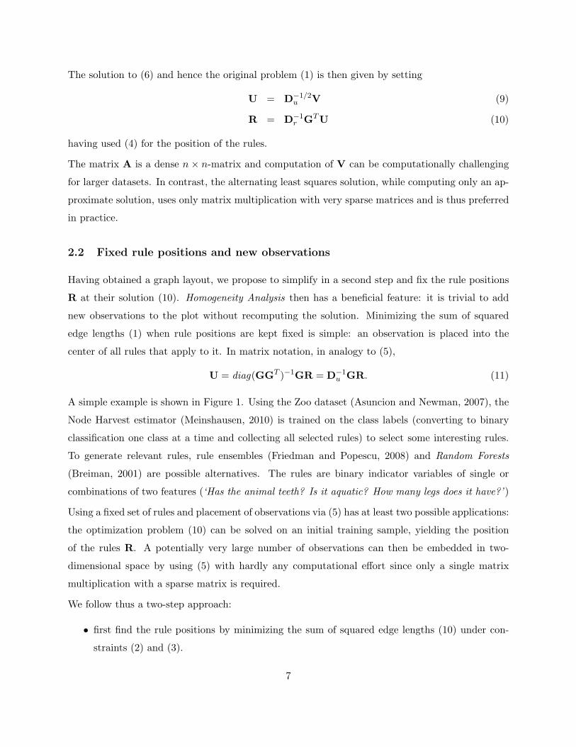
A simple example is shown in Figure 1. Using the Zoo dataset (Asuncion and Newman, 2007), the

Node Harvest estimator (Meinshausen, 2010) is trained on the class labels (converting to binary

classification one class at a time and collecting all selected rules) to select some interesting rules.

To generate relevant rules, rule ensembles (Friedman and Popescu, 2008) and Random Forests

(Breiman, 2001) are possible alternatives. The rules are binary indicator variables of single or

combinations of two features (‘Has the animal teeth? Is it aquatic? How many legs does it have?’ )

Using a fixed set of rules and placement of observations via (5) has at least two possible applications:

the optimization problem (10) can be solved on an initial training sample, yielding the position

of the rules R. A potentially very large number of observations can then be embedded in two-

dimensional space by using (5) with hardly any computational e!ort since only a single matrix

multiplication with a sparse matrix is required.

We follow thus a two-step approach:

• first find the rule positions by minimizing the sum of squared edge lengths (10) under con-

straints (2) and (3).

7

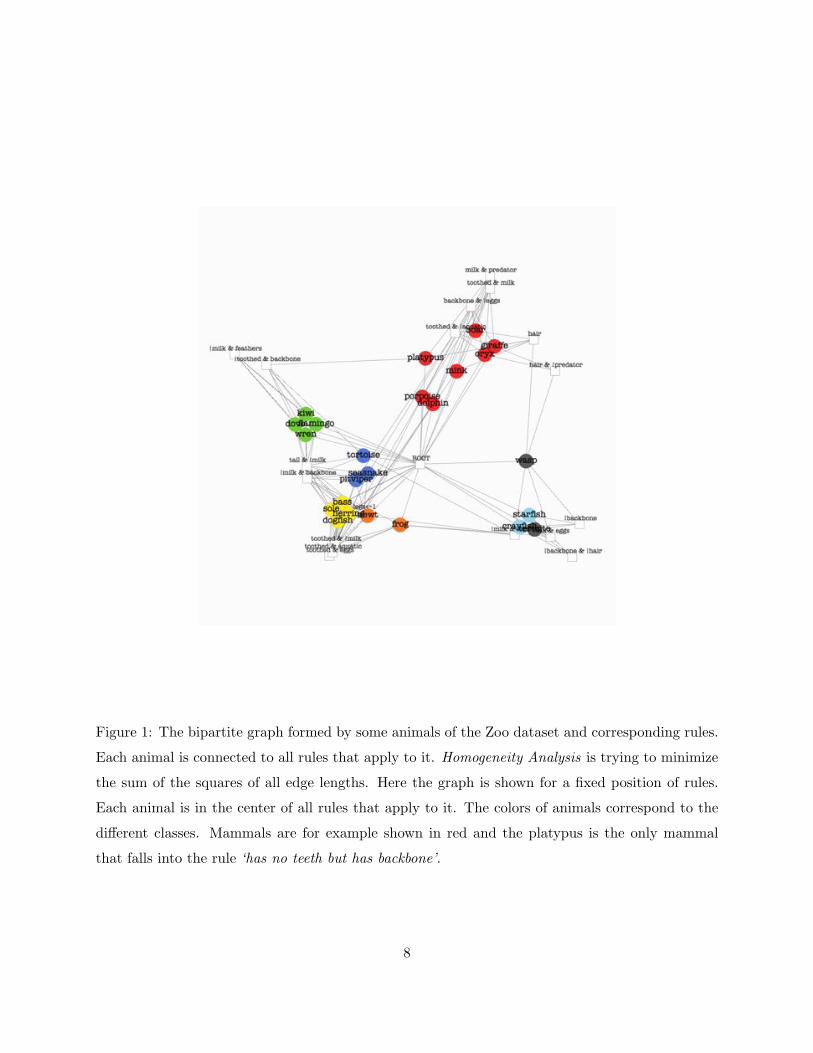
Figure 1: The bipartite graph formed by some animals of the Zoo dataset and corresponding rules.

Each animal is connected to all rules that apply to it. Homogeneity Analysis is trying to minimize

the sum of the squares of all edge lengths. Here the graph is shown for a fixed position of rules.

Each animal is in the center of all rules that apply to it. The colors of animals correspond to the

di!erent classes. Mammals are for example shown in red and the platypus is the only mammal

that falls into the rule ‘has no teeth but has backbone’.

8

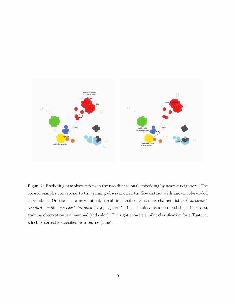
Figure 2: Predicting new observations in the two-dimensional embedding by nearest neighbors. The

colored samples correspond to the training observation in the Zoo dataset with known color-coded

class labels. On the left, a new animal, a seal, is classified which has characteristics {‘backbone’,

‘toothed’, ‘milk’, ‘no eggs’, ‘at most 1 leg’, ‘aquatic’}. It is classified as a mammal since the closest

training observation is a mammal (red color). The right shows a similar classification for a Tuatara,

which is correctly classified as a reptile (blue).

9

• then fix the rule positions and place all observations U by minimizing again the sum of

squared edge lengths (10): each observation is placed into the center of all rules that apply

to it.

A potential alternative would be to minimize directly criterion (10) but putting constraints on the

rules instead of the samples. Then (11) would apply directly to all observations. In practice, both

approaches yield very similar results and we chose the former since it allows an easier generalization

to Partition Maps.

It is of interest to measure, at least crudely, the amount of information that is lost in the two-

dimensional embedding. To be more precise, we want to quantify how much of the predictive

accuracy is lost when embedding observations in a low, typically two-dimensional space, using

Homogeneity Analysis.

This is achieved with the following steps.

Given: a set of training observations (Xi, Yi), i ! Itrain and test observations (Xi, Yi), i ! Itest.

1. Train the initial method such as Random Forests, Rule ensemble or Node Harvest (Breiman,

2001; Friedman and Popescu, 2008; Meinshausen, 2010) on the training observations and

extract all used m rules; these are all leaf nodes in the case of Random Forests and all rules

with non-zero weight for Rule Ensembles and Node Harvest.

2. Construct the sparse binary n"m indicator matrix G. The entry Gij is 1 if observation i is

falling into the j-th rule and 0 otherwise.

3. Compute the q-dimensional embedding of the rules R with the training set of observations

Itrain using (10) or alternating least squares. Fix these positions in the following.

4. Compute the positions U of the observations in both the training and test set via (5). Predict

class labels for all observations in the test set by nearest neighbor with Euclidean distance in

the q-dimensional embedding, using the training data (Ui, Yi), i ! Itrain as training data.

An example is given in Figure 2. The colored observations correspond to the observations in the

training dataset with a very small amount of jitter added for better visualization. Color indicates

the class and the same colors as in Figure 4 are used. The two test examples of seal (mammal)

and tuatara (reptile) can easily be correctly classified by positioning them in the 2-dimensional

embedding.

10

Figure 3: European Parliamentary votes visualization. Left: Training a Random Forests classifier

to distinguish between parties, non-metric multidimensional scaling was applied to the training

data. Right: using the same RF, the Homogenity Analysis solution with all embedded rules is

shown. Colors indicate party membership.

2.3 Example: European parliamentary votes

Data on voting behavior of Members of the European Parliament (MEP) has been collected in

Hix et al. (2006). Looking at the fifth parliament from 1999-2004, there have been 5745 votes. In

each vote, each of the 696 members can do one of the following five possibilities: vote yes, vote no,

abstain, be present but not vote, be absent.

Here, we are interested in the question whether party membership can be inferred from voting

behavior. This allows to answer a range of questions. Is each party showing a distinct voting

pattern? How homogeneous is the voting behavior in each party? Are there MEPs that are clearly

voting like members of another party (outliers)? Are there subgroups within parties? We will also

be looking at whether country of origin of MEPs can be inferred from voting behaviour (it can to

some extent, but cohesion is much weaker). There are 8 main parties: European Peoples Party

(shown as light blue), European Conservatives and Reformists (dark blue), Liberals (yellow), Greens

(green), Progressive Alliance of Socialists and Democrats (red), European United Left (orange) and

Europe for Freedom and Democracy (brown), of which the UK independence party is a member.

There are also non-inscrits (black), including mostly right-wing nationalistic parties.

11

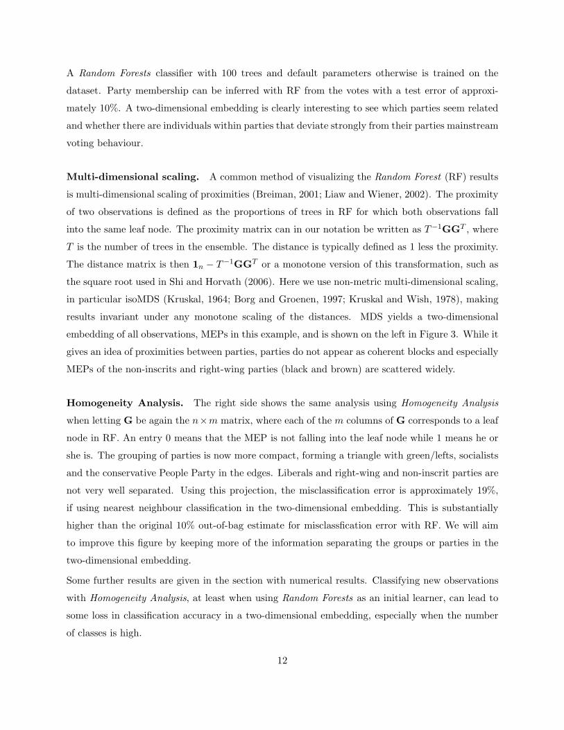
A Random Forests classifier with 100 trees and default parameters otherwise is trained on the

dataset. Party membership can be inferred with RF from the votes with a test error of approxi-

mately 10%. A two-dimensional embedding is clearly interesting to see which parties seem related

and whether there are individuals within parties that deviate strongly from their parties mainstream

voting behaviour.

Multi-dimensional scaling. A common method of visualizing the Random Forest (RF) results

is multi-dimensional scaling of proximities (Breiman, 2001; Liaw and Wiener, 2002). The proximity

of two observations is defined as the proportions of trees in RF for which both observations fall

into the same leaf node. The proximity matrix can in our notation be written as T!1GGT , where

T is the number of trees in the ensemble. The distance is typically defined as 1 less the proximity.

The distance matrix is then 1n % T!1GGT or a monotone version of this transformation, such as

the square root used in Shi and Horvath (2006). Here we use non-metric multi-dimensional scaling,

in particular isoMDS (Kruskal, 1964; Borg and Groenen, 1997; Kruskal and Wish, 1978), making

results invariant under any monotone scaling of the distances. MDS yields a two-dimensional

embedding of all observations, MEPs in this example, and is shown on the left in Figure 3. While it

gives an idea of proximities between parties, parties do not appear as coherent blocks and especially

MEPs of the non-inscrits and right-wing parties (black and brown) are scattered widely.

Homogeneity Analysis. The right side shows the same analysis using Homogeneity Analysis

when letting G be again the n"m matrix, where each of the m columns of G corresponds to a leaf

node in RF. An entry 0 means that the MEP is not falling into the leaf node while 1 means he or

she is. The grouping of parties is now more compact, forming a triangle with green/lefts, socialists

and the conservative People Party in the edges. Liberals and right-wing and non-inscrit parties are

not very well separated. Using this projection, the misclassification error is approximately 19%,

if using nearest neighbour classification in the two-dimensional embedding. This is substantially

higher than the original 10% out-of-bag estimate for misclassfication error with RF. We will aim

to improve this figure by keeping more of the information separating the groups or parties in the

two-dimensional embedding.

Some further results are given in the section with numerical results. Classifying new observations

with Homogeneity Analysis, at least when using Random Forests as an initial learner, can lead to

some loss in classification accuracy in a two-dimensional embedding, especially when the number

of classes is high.

12

3 Partition Map

We believe that Homogeneity Analysis has great potential for e!ective visualizations of tree en-

sembles and similar machine learning algorithms. There are two potential shortcomings of this

approach: computational issues can arise if the number of training observations is very large.

More importantly, the predictive accuracy in a two-dimensional embedding is sometimes notice-

ably worse than with the original tree ensemble, which means that crucial information is lost by

the low-dimensional embedding.

We propose a simple extension of Homogeneity Analysis, called Partition Map, that partially ad-

dresses these two shortcomings for multiclass classification, where Y ! {1, . . . ,K}, and can lead to

noticeable improvements in predictive accuracy.

3.1 Grouping observations across classes

The only di!erence to Homogeneity Analysis as discussed above is that we initially group all

observations of a single class. This yields a di!erent positioning of the rules. Once the rules

are positioned, we proceed just as before. This change will allow for faster computations but,

more importantly, for a better separation between classes in the low-dimensional embedding. A

grouping of the observations for each class in (10) is enforced by requiring that Ui = Ui! for all

i, i" ! {1, . . . , n} for which Yi = Yi! . Let Uk be the position of the k-th class for k = 1, . . . ,K. Let

the K "m indicator matrix G be the aggregate matrix of G, where the aggregation happens over

the K classes,

Gkm =%

i:Yi=k

Gij . (12)

Under this constraint, the corresponding optimization problem to Homogeneity Analysis (1) with

constraints (2) is then

argminU,R

K%

k=1

m%

j=1

Gkm$Uk %Rj$22 (13)

such that UT diag(GGT )U = 1q (14)

and eTKU = 0. (15)

The solution can be conveniently obtained completely analogous to the eigenvalue approach to

Homogeneity Analysis. Let Du = diag(GGT ) and Dr = diag(GT G) and

A := D!1/2u ST

K(GD!1r GT )SKD!1/2

u (16)

13

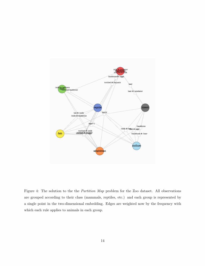
Figure 4: The solution to the the Partition Map problem for the Zoo dataset. All observations

are grouped according to their class (mammals, reptiles, etc.) and each group is represented by

a single point in the two-dimensional embedding. Edges are weighted now by the frequency with

which each rule applies to animals in each group.

14

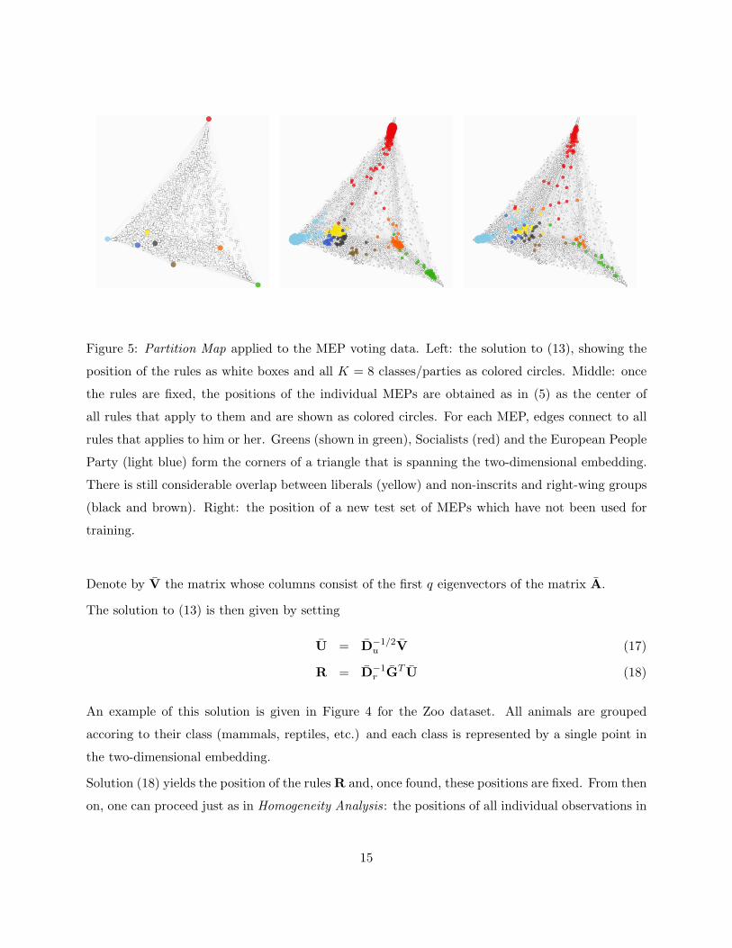
Figure 5: Partition Map applied to the MEP voting data. Left: the solution to (13), showing the

position of the rules as white boxes and all K = 8 classes/parties as colored circles. Middle: once

the rules are fixed, the positions of the individual MEPs are obtained as in (5) as the center of

all rules that apply to them and are shown as colored circles. For each MEP, edges connect to all

rules that applies to him or her. Greens (shown in green), Socialists (red) and the European People

Party (light blue) form the corners of a triangle that is spanning the two-dimensional embedding.

There is still considerable overlap between liberals (yellow) and non-inscrits and right-wing groups

(black and brown). Right: the position of a new test set of MEPs which have not been used for

training.

Denote by V the matrix whose columns consist of the first q eigenvectors of the matrix A.

The solution to (13) is then given by setting

U = D!1/2u V (17)

R = D!1r GT U (18)

An example of this solution is given in Figure 4 for the Zoo dataset. All animals are grouped

accoring to their class (mammals, reptiles, etc.) and each class is represented by a single point in

the two-dimensional embedding.

Solution (18) yields the position of the rules R and, once found, these positions are fixed. From then

on, one can proceed just as in Homogeneity Analysis: the positions of all individual observations in

15

both training and test data are found as in (5) as the center of all rules the observation falls into:

U = diag(GGT )!1GR.

For the Zoo dataset, Figure 1 shows the combined position of rules and observations after this step.

The predictive accuracy can then be evaluated just as for Homogeneity Analysis.

The entire Partition Map algorithm is then as follows.

1. Train the initial method on the training observations and extract all m used rules/leaf nodes

to from the n"m binary indicator matrix G. Aggregate rows by class membership as in (12)

to obtain G.

2. Compute the q-dimensional embedding of the rules R using (18).

3. Compute the positions U of the observations (for either training or test data) as U =

diag(GGT )!1GR.

Results for the European Parliamentary vote data are shown in Figure 5. The predictive accuracy of

nearest neighbours is now 17%, improving slightly upon Homogeneity Analysis. Another advantage

over Homogeneity Analysis is computational: the eigenvalues decomposition has to be performed

only on an K "m matrix with K = 8 instead of a n " n matrix with n = 696. It is also faster

than the alternating least squares for Homogeneity Analysis but the main advantage is the better

quality of the embedding, both measured subjectively by visual inspection as well as in predictive

accuracy.

3.2 Force-based layout

The unique feature of the Partition Map algorithm is that observations of a single class are grouped

together when computing the embedding of the rules. This is yielding computational savings but

is more importantly leading to a layout which gives better separation between classes. Yet class

separation is still not quite as accurate as with the underying Random Forest. The main cause

is the partial overlap between classes when looking for the best positioning of the rules. The

variance-based constraint (14) does not penalize overlap between classes.

For the following, it is worth to attach a geometric interpretation to the objective function (13).

Minimizing the sum of the squared distances between observations and rules can be thought of as

16

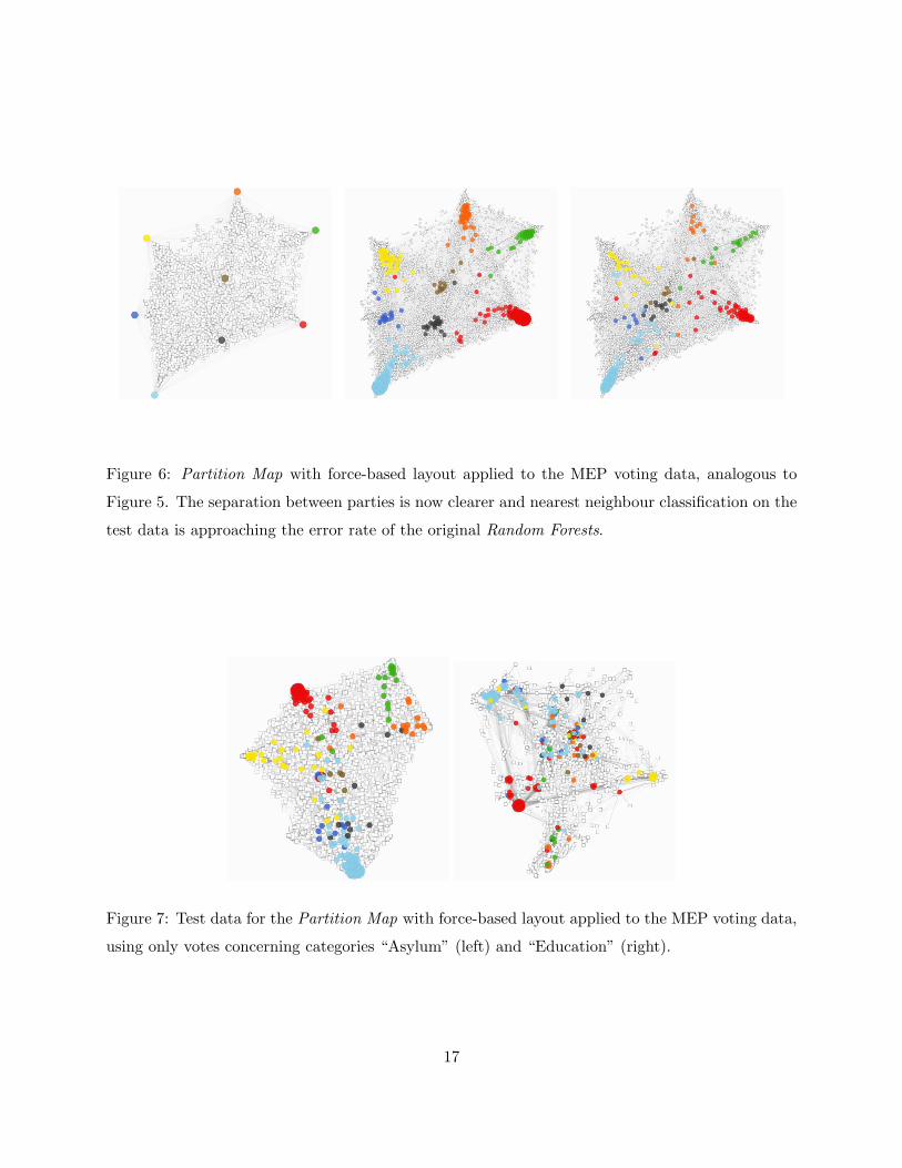
Figure 6: Partition Map with force-based layout applied to the MEP voting data, analogous to

Figure 5. The separation between parties is now clearer and nearest neighbour classification on the

test data is approaching the error rate of the original Random Forests.

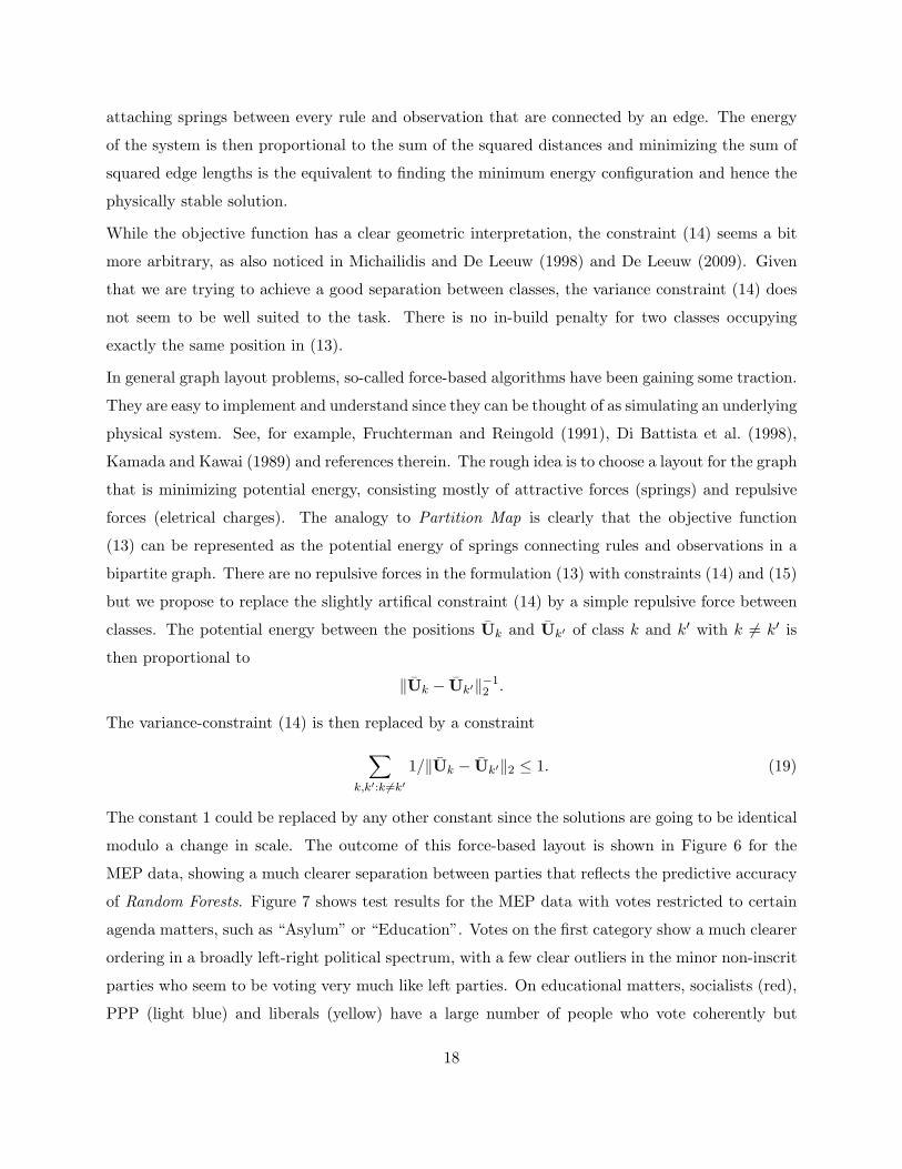
Figure 7: Test data for the Partition Map with force-based layout applied to the MEP voting data,

using only votes concerning categories “Asylum” (left) and “Education” (right).

17

attaching springs between every rule and observation that are connected by an edge. The energy

of the system is then proportional to the sum of the squared distances and minimizing the sum of

squared edge lengths is the equivalent to finding the minimum energy configuration and hence the

physically stable solution.

While the objective function has a clear geometric interpretation, the constraint (14) seems a bit

more arbitrary, as also noticed in Michailidis and De Leeuw (1998) and De Leeuw (2009). Given

that we are trying to achieve a good separation between classes, the variance constraint (14) does

not seem to be well suited to the task. There is no in-build penalty for two classes occupying

exactly the same position in (13).

In general graph layout problems, so-called force-based algorithms have been gaining some traction.

They are easy to implement and understand since they can be thought of as simulating an underlying

physical system. See, for example, Fruchterman and Reingold (1991), Di Battista et al. (1998),

Kamada and Kawai (1989) and references therein. The rough idea is to choose a layout for the graph

that is minimizing potential energy, consisting mostly of attractive forces (springs) and repulsive

forces (eletrical charges). The analogy to Partition Map is clearly that the objective function

(13) can be represented as the potential energy of springs connecting rules and observations in a

bipartite graph. There are no repulsive forces in the formulation (13) with constraints (14) and (15)

but we propose to replace the slightly artifical constraint (14) by a simple repulsive force between

classes. The potential energy between the positions Uk and Uk! of class k and k" with k &= k" is

then proportional to

$Uk % Uk!$!12 .

The variance-constraint (14) is then replaced by a constraint

%

k,k!:k #=k!

1/$Uk % Uk!$2 ' 1. (19)

The constant 1 could be replaced by any other constant since the solutions are going to be identical

modulo a change in scale. The outcome of this force-based layout is shown in Figure 6 for the

MEP data, showing a much clearer separation between parties that reflects the predictive accuracy

of Random Forests. Figure 7 shows test results for the MEP data with votes restricted to certain

agenda matters, such as “Asylum” or “Education”. Votes on the first category show a much clearer

ordering in a broadly left-right political spectrum, with a few clear outliers in the minor non-inscrit

parties who seem to be voting very much like left parties. On educational matters, socialists (red),

PPP (light blue) and liberals (yellow) have a large number of people who vote coherently but

18

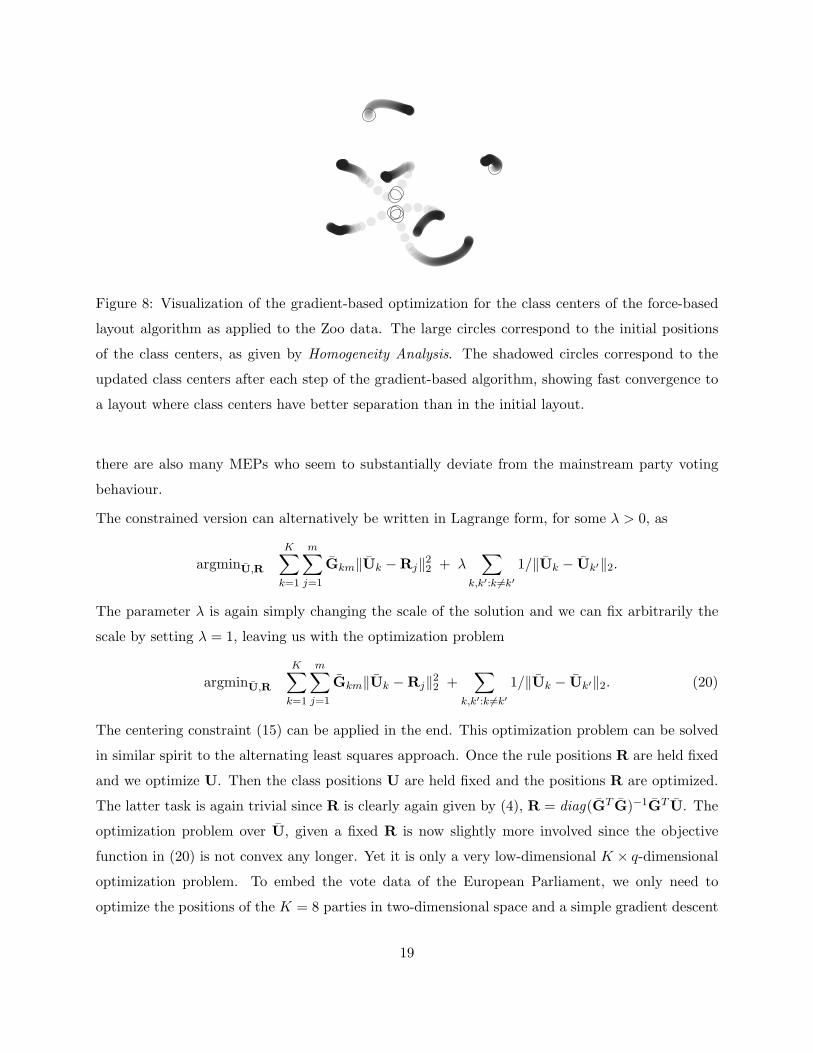
Figure 8: Visualization of the gradient-based optimization for the class centers of the force-based

layout algorithm as applied to the Zoo data. The large circles correspond to the initial positions

of the class centers, as given by Homogeneity Analysis. The shadowed circles correspond to the

updated class centers after each step of the gradient-based algorithm, showing fast convergence to

a layout where class centers have better separation than in the initial layout.

there are also many MEPs who seem to substantially deviate from the mainstream party voting

behaviour.

The constrained version can alternatively be written in Lagrange form, for some " > 0, as

argminU,R

K%

k=1

m%

j=1

Gkm$Uk %Rj$22 + "%

k,k!:k #=k!

1/$Uk % Uk!$2.

The parameter " is again simply changing the scale of the solution and we can fix arbitrarily the

scale by setting " = 1, leaving us with the optimization problem

argminU,R

K%

k=1

m%

j=1

Gkm$Uk %Rj$22 +%

k,k!:k #=k!

1/$Uk % Uk!$2. (20)

The centering constraint (15) can be applied in the end. This optimization problem can be solved

in similar spirit to the alternating least squares approach. Once the rule positions R are held fixed

and we optimize U. Then the class positions U are held fixed and the positions R are optimized.

The latter task is again trivial since R is clearly again given by (4), R = diag(GT G)!1GT U. The

optimization problem over U, given a fixed R is now slightly more involved since the objective

function in (20) is not convex any longer. Yet it is only a very low-dimensional K " q-dimensional

optimization problem. To embed the vote data of the European Parliament, we only need to

optimize the positions of the K = 8 parties in two-dimensional space and a simple gradient descent

19

algorithm is su"cient. There could potentially be several local minima, although it is not very

common as long as the number of classes is low enough. However, we always start from the

Partition Map solution to (13) given in (18) and search for the nearest local minimum by gradient

descent.

Convergence is defined in our simulations as being achieved in iteration l ! N i! the relative change

in Euclidean distance between the position U in iteration l and l + 1 is less than a tolerance value

of 10!6. Convergence is typically very fast since, as mentioned above, the optimization is only

over the K " q-matrix of the positions of the K classes in q-dimensional space, so typically a

K " 2-dimensional optimization problem. Here, a very simple gradient-descent based algorithms

is employed. Starting from the solution to the Partition Map solution (13), the positions U of the

class centers are updated in the direction of the gradient of (20), using a step-length that starts

as 1/10th the square root of the mean squared distance between class centers in (13) and decays

geometrically with a decay of 0.99 over the number of iterations. After each update of the positions

U, the rule positions R are re-computed using R = diag(GT G)!1GT U.

The force-based Partition Map algorithm.

1. Train the initial method on the training observations and extract all m used rules/leaf nodes

to from the n"m binary indicator matrix G. Aggregate rows by class membership as in (12)

to obtain G.

2. Compute the q-dimensional embedding of the rules R using (18).

3. Iterate the following two steps until convergence.

(a) Optimize the K positions U of the classes by a gradient descent of the objective function

in (20), keeping the positions of the rules R fixed.

(b) Compute the position of the rules as R = diag(GT G)!1GT U.

4. Center the observations by setting U( SKU and let again R = diag(GT G)!1GT U.

5. Compute the positions U of all observations (for either training or test data) as U =

diag(GGT )!1GR.

An example of the gradient-based algorithm is given in Figure 8 for the Zoo data, showing the

convergence of the class centers from an initial layout given by Homogeneity Analysis to a layout

20

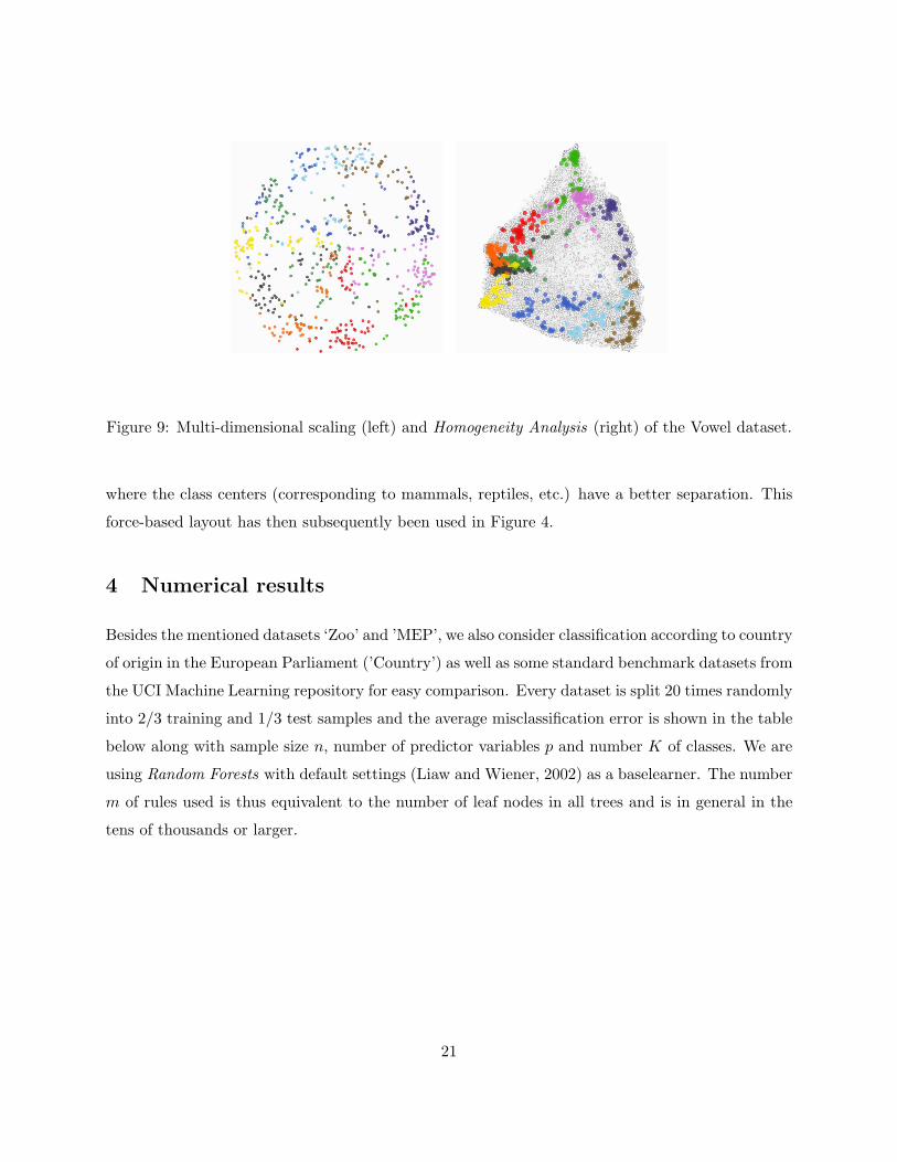
Figure 9: Multi-dimensional scaling (left) and Homogeneity Analysis (right) of the Vowel dataset.

where the class centers (corresponding to mammals, reptiles, etc.) have a better separation. This

force-based layout has then subsequently been used in Figure 4.

4 Numerical results

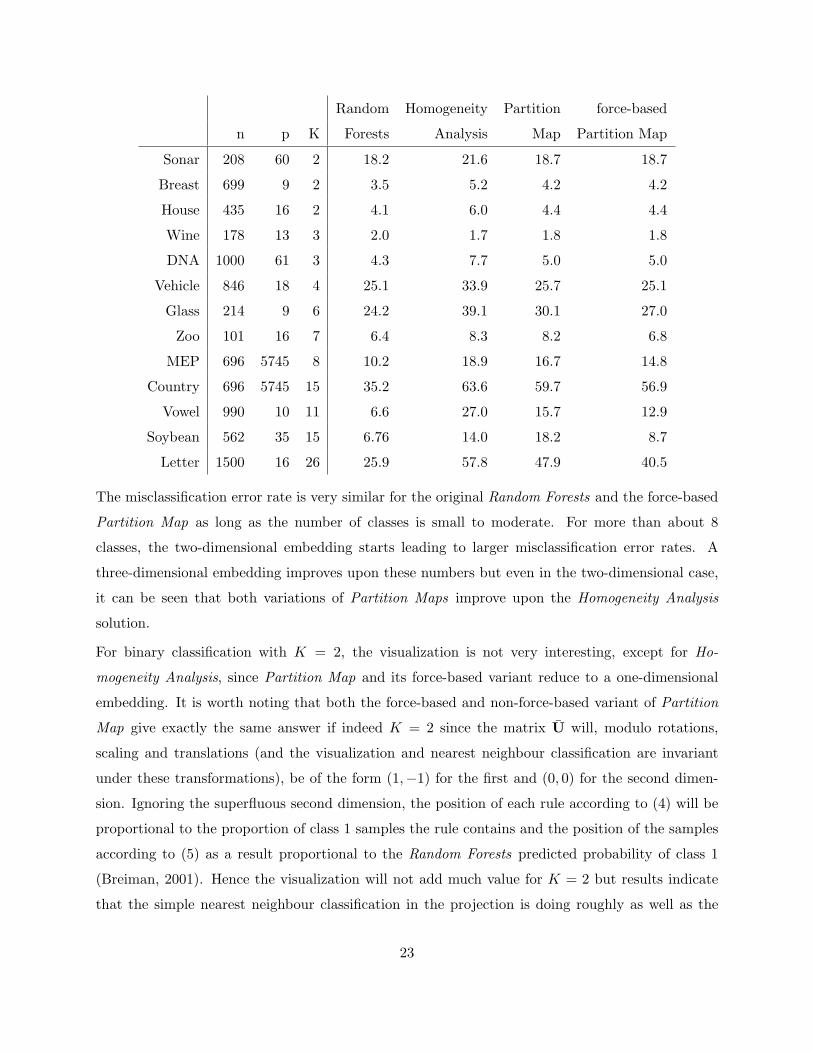
Besides the mentioned datasets ‘Zoo’ and ’MEP’, we also consider classification according to country

of origin in the European Parliament (’Country’) as well as some standard benchmark datasets from

the UCI Machine Learning repository for easy comparison. Every dataset is split 20 times randomly

into 2/3 training and 1/3 test samples and the average misclassification error is shown in the table

below along with sample size n, number of predictor variables p and number K of classes. We are

using Random Forests with default settings (Liaw and Wiener, 2002) as a baselearner. The number

m of rules used is thus equivalent to the number of leaf nodes in all trees and is in general in the

tens of thousands or larger.

21

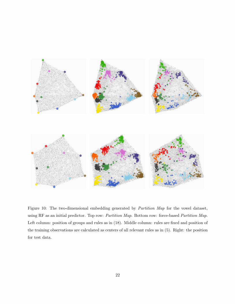
Figure 10: The two-dimensional embedding generated by Partition Map for the vowel dataset,

using RF as an initial predictor. Top row: Partition Map. Bottom row: force-based Partition Map.

Left column: position of groups and rules as in (18). Middle column: rules are fixed and position of

the training observations are calculated as centers of all relevant rules as in (5). Right: the position

for test data.

22

Random Homogeneity Partition force-based

n p K Forests Analysis Map Partition Map

Sonar 208 60 2 18.2 21.6 18.7 18.7

Breast 699 9 2 3.5 5.2 4.2 4.2

House 435 16 2 4.1 6.0 4.4 4.4

Wine 178 13 3 2.0 1.7 1.8 1.8

DNA 1000 61 3 4.3 7.7 5.0 5.0

Vehicle 846 18 4 25.1 33.9 25.7 25.1

Glass 214 9 6 24.2 39.1 30.1 27.0

Zoo 101 16 7 6.4 8.3 8.2 6.8

MEP 696 5745 8 10.2 18.9 16.7 14.8

Country 696 5745 15 35.2 63.6 59.7 56.9

Vowel 990 10 11 6.6 27.0 15.7 12.9

Soybean 562 35 15 6.76 14.0 18.2 8.7

Letter 1500 16 26 25.9 57.8 47.9 40.5

The misclassification error rate is very similar for the original Random Forests and the force-based

Partition Map as long as the number of classes is small to moderate. For more than about 8

classes, the two-dimensional embedding starts leading to larger misclassification error rates. A

three-dimensional embedding improves upon these numbers but even in the two-dimensional case,

it can be seen that both variations of Partition Maps improve upon the Homogeneity Analysis

solution.

For binary classification with K = 2, the visualization is not very interesting, except for Ho-

mogeneity Analysis, since Partition Map and its force-based variant reduce to a one-dimensional

embedding. It is worth noting that both the force-based and non-force-based variant of Partition

Map give exactly the same answer if indeed K = 2 since the matrix U will, modulo rotations,

scaling and translations (and the visualization and nearest neighbour classification are invariant

under these transformations), be of the form (1,%1) for the first and (0, 0) for the second dimen-

sion. Ignoring the superfluous second dimension, the position of each rule according to (4) will be

proportional to the proportion of class 1 samples the rule contains and the position of the samples

according to (5) as a result proportional to the Random Forests predicted probability of class 1

(Breiman, 2001). Hence the visualization will not add much value for K = 2 but results indicate

that the simple nearest neighbour classification in the projection is doing roughly as well as the

23

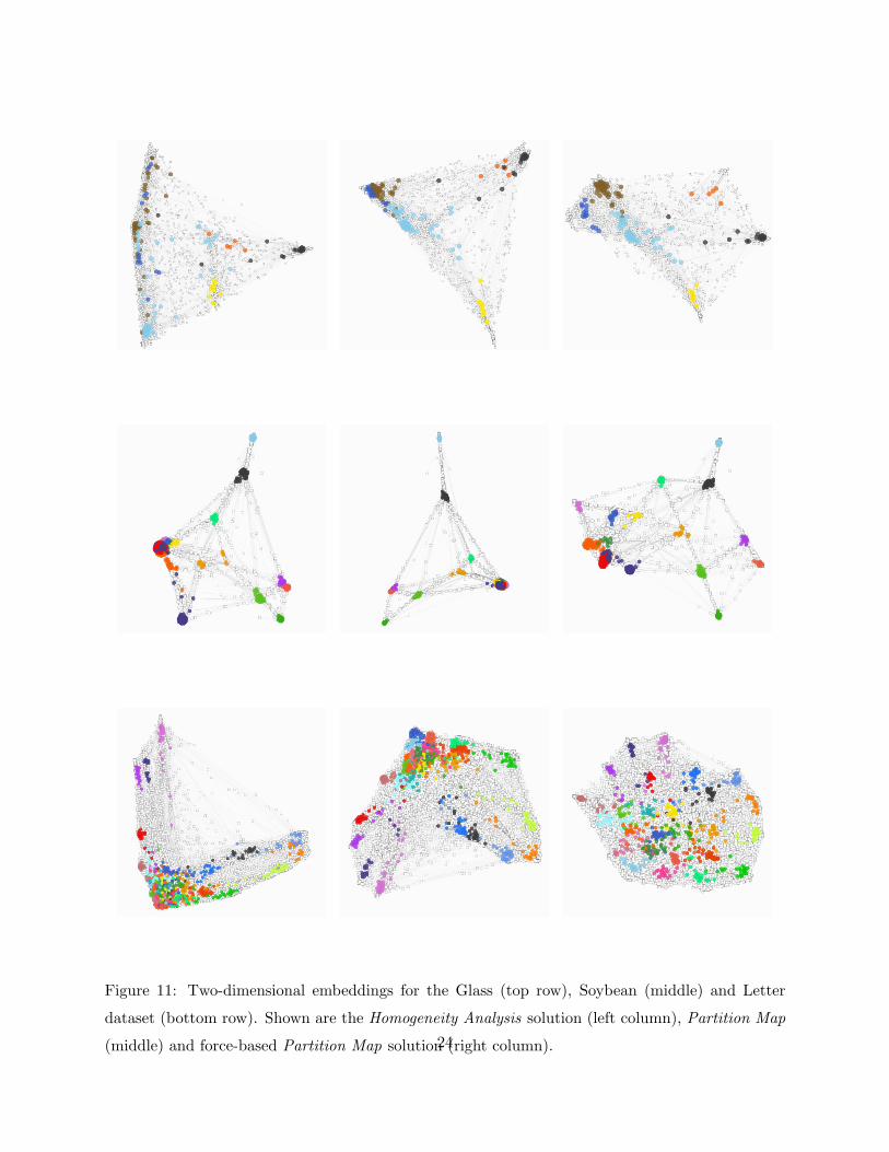
Figure 11: Two-dimensional embeddings for the Glass (top row), Soybean (middle) and Letter

dataset (bottom row). Shown are the Homogeneity Analysis solution (left column), Partition Map

(middle) and force-based Partition Map solution (right column).24

original RF procedure for all datasets with K = 2.

The more interesting datasets contain at least three classes. In general, the nearest neighbour pre-

diction accuracy with forced-based Prediction Map is close to the accuracy of the original Random

Forests, at least as long as the number of classes is less or equal to 7. For more classes, it seems

increasingly hard to find a two-dimensional embedding that preserves all information of Random

Forests and the misclassification error rate is dropping as a result.

To show another example, Figure 9 contains the MDS and Homogeneity Analysis solutions for the

11-class vowel dataset (Asuncion and Newman, 2007). The non-metric MDS solution shows again

large overlap of classes and Homogeneity Analysis, when using Random Forests as an initial learner,

is improving upon it. The Partition Map solutions are shown in Figure 10 and the separation

between classes is improved again, both for training as well as test data. Between the two variations

of Partition Map, the force-based algorithm is again showing the best performance. It allows

exploratory analysis of predicttion results, helps in the search for outliers and potential sub-groups

and helps to discover potentially interesting relations between classes.

5 Discussion

Tree ensembles and related procedures provide typically very accurate predictions. Sometimes,

these predictions are su"cient. Often, however, a researcher or practitioner might be interest in

questions that go beyond accurate prediction. Visualization of tree ensembles, especially Random

Forests, can aid in interpreting the results of multiclass classification problems and helps to answer

questions such as: which classes are related and similar to each other? Are there subgroups within

classes? Are there outlying observations?

Partition Maps is leveraging ideas from Homogeneity Analysis to give a low-dimensional embedding

of all observations together with all rules or leaf nodes of the original tree ensemble. A bipartite

graph is first formed, where each observation is connected to each rule that applied to it and the

layout is minimizing the sum of the squared distances in this bipartite graph.

The optimization problem is very fast to compute and results are encouraging: class separation is

very accurate and very similar to the accuracy of the underlying Random Forests procedure, at

least as long as the number of classes is not exceedingly large. While not covered, it is conceivable

that similar ideas also apply to regression and unsupervised learning with Random Forests (Shi

and Horvath, 2006).

25

Partition Maps can thus be potentially useful by providing a fast and intuitive way to achieve a

low-dimensional embedding of the data and answer queries about subgroups, proximities between

classes and outlying observations.

References

Asuncion, A. and D. Newman (2007). UCI machine learning repository.

Borg, I. and P. Groenen (1997). Modern multidimensional scaling: Theory and applications.

Springer Verlag.

Breiman, L. (1996). Bagging predictors. Machine Learning 24, 123–140.

Breiman, L. (2001). Random Forests. Machine Learning 45, 5–32.

Breiman, L., J. Friedman, R. Olshen, and C. Stone (1984). Classification and Regression Trees.

Wadsworth, Belmont.

De Leeuw, J. (1988). Convergence of the majorization method for multidimensional scaling. Journal

of classification 5, 163–180.

De Leeuw, J. (2009). Beyond homogeneity analysis. Technical report, UCLA.

De Leeuw, J. and P. Mair (2008). Homogeneity Analysis in R: The package homals. Journal of

Statistical Software.

Di Battista, G., P. Eades, R. Tamassia, and I. Tollis (1998). Graph drawing: algorithms for the

visualization of graphs. Prentice Hall, NJ, USA.

Friedman, J. and B. Popescu (2008). Predictive learning via rule ensembles. Annals of Applied

Statistics 2, 916–954.

Fruchterman, T. and E. Reingold (1991). Graph drawing by force-directed placement. Software-

Practice and Experience 21, 1129–1164.

Goldberger, J., S. Roweis, G. Hinton, and R. Salakhutdinov (2005). Neighbourhood components

analysis. Advances in neural information processing systems 17, 513–520.

Gower, J. and D. Hand (1996). Biplots. Chapman & Hall/CRC.

26

Greenacre, M. and T. Hastie (1987). The geometric interpretation of correspondence analysis.

Journal of the American Statistical Association 82, 437–447.

Hix, S., A. Noury, and G. Roland (2006). Dimensions of politics in the European Parliament.

American Journal of Political Science 50, 494–511.

Kamada, T. and S. Kawai (1989). An algorithm for drawing general undirected graphs. Information

processing letters 31, 7–15.

Kruskal, J. (1964). Nonmetric multidimensional scaling: a numerical method. Psychometrika 29,

115–129.

Kruskal, J. and M. Wish (1978). Multidimensional scaling. Sage Publications, Inc.

Liaw, A. and M. Wiener (2002). Classication and regression by randomForest. R News 2, 18–22.

Lin, Y. and Y. Jeon (2006). Random forests and adaptive nearest neighbors. Journal of the

American Statistical Association 101, 578–590.

Meinshausen, N. (2010). Node harvest. Arxiv preprint arXiv:0910.2145, to appear in Annals of

Applied Statistics.

Meulman, J. (1982). Homogeneity analysis of incomplete data. DSWO Press.

Michailidis, G. and J. De Leeuw (1998). The Gifi system of descriptive multivariate analysis.

Statistical Science, 307–336.

Roweis, S. and L. Saul (2000). Nonlinear dimensionality reduction by locally linear embedding.

Science 290, 2323.

Shi, T. and S. Horvath (2006). Unsupervised learning with random forest predictors. Journal of

Computational and Graphical Statistics 15, 118–138.

Sugiyama, M. (2007). Dimensionality reduction of multimodal labeled data by local Fisher dis-

criminant analysis. The Journal of Machine Learning Research 8, 1061.

Tenenbaum, J., V. Silva, and J. Langford (2000). A global geometric framework for nonlinear

dimensionality reduction. Science 290, 2319.

27

Tenenhaus, M. and F. Young (1985). An analysis and synthesis of multiple correspondence analysis,

optimal scaling, dual scaling, homogeneity analysis and other methods for quantifying categorical

multivariate data. Psychometrika 50, 91–119.

Urbanek, S. (2008). Visualizing Trees and Forests. Handbook of Data Visualization, 243–264.

Weinberger, K. and L. Saul (2009). Distance metric learning for large margin nearest neighbor

classification. The Journal of Machine Learning Research 10, 207–244.

28