Embed Size (px)
Citation preview


PARTITION COEFFICIENTS FOR METALSIN SURFACE WATER, SOIL, AND WASTE
DRAFT
Work Assignment Manager Robert B. Ambrose, Jr., P.E.and Technical Direction: U.S. Environmental Protection Agency
Office of Research and DevelopmentAthens, GA 30605
Prepared by: HydroGeoLogic, Inc1155 Herndon Parkway, Suite 900Herndon, VA 20170
and
Allison Geoscience Consultants, Inc.3920 Perry LaneFlowery Branch, GA 30542
Under Contract No. 68-C6-0020
U.S. Environmental Protection AgencyOffice of Solid Waste
Washington, DC 20460
June 22, 1999

TABLE OF CONTENTS
page
1.0 INTRODUCTION AND BACKGROUND . . . . . . . . . . . . . . . . . . . . . . . . 1-1
2.0 LITERATURE SURVEY FOR METAL PARTITION COEFFICIENTS . . . . . 2-1
3.0 ANALYSIS OF RETRIEVED DATA AND DEVELOPMENT OF PARTITION COEFFICIENT VALUES . . . . . . . . . . . . . . . . . . . . . . . . . . 3-13.1 DEVELOPMENT OF PARTITIONING COEFFICIENTS IN
NATURAL MEDIA . . . . . . . . . . . . . . . . . . . . . . . . . . . . . . . . . . 3-13.1.1 Estimation from Regression Equations Based on Literature Data . 3-23.1.2 Estimation From Geochemical Speciation Modeling . . . . . . . . . 3-33.1.3 Estimation from Expert Judgement . . . . . . . . . . . . . . . . . . . . 3-6
3.2 DEVELOPMENT OF PARTITIONING COEFFICIENTS FOR WASTE SYSTEMS . . . . . . . . . . . . . . . . . . . . . . . . . . . . . . . 3-153.2.1 Estimation from Analysis of Data Presented in the Literature . . . 3-163.2.2 Estimation from Geochemical Speciation Modeling . . . . . . . . . . 3-18
4.0 REFERENCES . . . . . . . . . . . . . . . . . . . . . . . . . . . . . . . . . . . . . . . . . 4-1
APPENDICES
APPENDIX A METAL PARTITION COEFFICIENTS USED IN SOME PREVIOUSU.S. EPA RISK ASSESSMENTS
APPENDIX B EXAMPLE INPUT FILE FOR THE MINTEQA2 MODEL USED TOESTIMATE PARTITIONING IN SOIL
APPENDIX C EXAMPLE INPUT FILE FOR THE MINTEQA2 MODEL USED TOESTIMATE PARTITIONING WITH DOC
APPENDIX D EXAMPLE INPUT FILE FOR THE MINTEQA2 MODEL USED TOESTIMATE PARTITIONING WITH WASTE SYSTEMS
LIST OF TABLES
page
Table 1 Median, range, and number of samples (N) for partition coefficients (log Kd in L/kg) from the literature search . . . . . . . . . . . . . . . . . . . . 2-3
Table 2 Linear Regression Equations used to Estimate Mean log Kd Values (L/kg) in Natural media . . . . . . . . . . . . . . . . . . . . . . . . . . . . . . . . 3-3
Table 3 Metal partition coefficients (log Kd) in kg/L for soil/soil water . . . . . . . 3-7Table 4 Metal partition coefficients (log Kd) in kg/L for sediment/porewater . . . . 3-9Table 5 Metal partition coefficients (log Kd) in kg/L for suspended matter/water . 3-11Table 6 Metal partition coefficients (log Kd) in kg/L for partitioning between
DOC and inorganic solution species . . . . . . . . . . . . . . . . . . . . . . . . 3-13Table 7 Effective partition coefficients based on reported solid phase and
solution phase metals concentrations from leach tests reported in the literature . . . . . . . . . . . . . . . . . . . . . . . . . . . . . . . . . . . . . . . 3-17
Table 8 Important parameters and constituent concentrations used in MINTEQA2 modeling of landfills in the acetogenic and methanogenic stages and MSWI and CKD monofills . . . . . . . . . . . . . . . . . . . . . . . . . . . . . . 3-19
Table 9 Estimated range in log partition coefficients (L/kg) for selected metals determined from MINTEQA2 modeling . . . . . . . . . . . . . . . . . . . . . . 3-20

1-1
1.0 INTRODUCTION AND BACKGROUND
The purpose of this study was to develop contaminant partition coefficients for the surfacewater pathway and for the source model used in the multimedia approach for the HazardousWaste Identification Rule (HWIR). Partition coefficients for certain metal contaminants inenvironmental media are needed to perform multimedia exposure and risk assessmentmodeling for HWIR. The multimedia model includes a surface water pathway model thatrequires partition coefficients to account for removal of contaminant from the solution phaseand retardation of contaminant movement. The contaminants of interest are the metals:antimony (Sb), arsenic (As), barium (Ba), beryllium (Be), cadmium (Cd), chromium (Cr),cobalt (Co), copper (Cu), lead (Pb), molybdenum (Mo), mercury (Hg), nickel (Ni), selenium(Se), silver (Ag), thallium (Tl), tin (Sn), vanadium (V), and zinc (Zn). Methylated mercury(CH3Hg+) and cyanide (CN) are also of interest. In the surface water pathway, the HWIRmodeling scenario includes several transport processes that require metal partitioncoefficients: (1) The overland transport of metal contaminants in runoff water in thewatershed and the consequent partitioning between soil and water; (2) partitioning betweenthe suspended load and the water in streams, rivers, and lakes; (3) partitioning betweenriverine or lacustrine sediment and its porewater; and (4) partitioning between dissolvedorganic carbon (DOC) and the inorganic solution species in the water of streams, rivers, andlakes.
The HWIR modeling scenario includes a source model for various types of waste managementunits that also requires partition coefficients. For the source model, the partition coefficientsare used to represent the ratio of contaminant mass in the solid phase to that in the leachate(water) phase. There are five types of waste management units for which the source modelrequires partition coefficients: land application units, waste piles, landfills, treatment lagoons(surface impoundments), and aerated tanks.
This report describes the two-phase approach used in developing the needed partitioncoefficients. In the preferred method of obtaining the coefficients, a literature survey wasperformed to determine the range and statistical distribution of values that have beenobserved in field scenarios. This includes the collection of published partition coefficientsfor any of the metals in any of the environmental media of interest, or the estimation ofpartition coefficients from reported metal concentration data when feasible. The dataretrieved in the literature search were recorded in a spreadsheet along with associatedgeochemical parameters (such as pH, sorbent content, etc.) when these were reported. It wasanticipated that the literature search would not supply partition coefficients for all of themetals in all of the environmental media of interest. In the second-phase effort, statisticalmethods, geochemical speciation modeling, and expert judgement were used to providereasonable estimates of partition coefficients not available from the literature.

2-1
2.0 LITERATURE SURVEY FOR METAL PARTITION COEFFICIENTS
A literature survey was conducted to obtain partition coefficients to describe the partitioningof metals between soil and soil-water, between suspended particulate matter (SPM) andsurface water, between sediment and sediment-porewater, and between DOC and thedissolved inorganic phase in natural waters. In addition, partition coefficients were soughtfor equilibrium partitioning of metals between waste matrix material and the associatedaqueous phase in land application units, waste piles, landfills, treatment lagoons, and aeratedtanks. The literature survey encompassed periodical scientific and engineering materials andsome non-periodicals including books and technical reports published by the U.S. EPA andother government agencies. Electronic searches of the following databases were included aspart of the literature survey:
• Academic Press Journals (1995 - present)• AGRICOLA (1970 - present)• Analytical Abstracts (1980 - present)• Applied Science and Technology Abstracts • Aquatic Sciences and Fisheries Abstract Set (1981 - present) • CAB Abstracts (1987 - present)• Current Contents (1992 - present)• Dissertation Abstracts (1981 - present)• Ecology Abstracts (1982 - present)• EIS Digest of Environmental Impact Statements (1985 - present)• EI Tech Index (1987 - present)• Environmental Engineering Abstracts (1990 - present)• General Science Abstracts (1984 - present)• GEOBASE (1980 - present)• GEOREF (1785 - present)• National Technical Information Service • PapersFirst (1993 - present)• Periodical Abstracts (1986 - present)• Toxicology Abstracts (1982 - present)• Water Resources Abstracts (1987 - present)
Two search strings were used in the electronic searches: ”distribution coefficient” and“partition coefficient”. Use of such general strings has the advantage of generating manycitations, decreasing the probability that relevant articles will be missed, but also carrying ahigh labor burden because each citation returned must be examined for useful data. Formetals that are not as well represented in the published literature, even more general searchstrings were used, sometimes with boolean operators (e.g., “barium” and “soil”, “selenium”and “partitioning”). The work of identifying articles containing useful data from among allthose retrieved was made easier by first reviewing the titles to eliminate those of obviousirrelevance, then reviewing the abstracts, which were usually available on-line. Abstracts ofcitations that showed promise for providing partition coefficients were printed and given a

2-2
code consisting of the first two letters of the lead author’s last name and the last two digits ofthe year of publication. The code, along with the first few words of the article title, wasentered in a log book for tracking. Logged articles were quickly reviewed at local universityresearch libraries, and those containing relevant data were copied for a more thorough reviewat the office. Most of the articles were obtained from the University of Georgia ScienceLibrary or the Georgia Institute of Technology Library. As each copied article or report wasreviewed, a summary page containing the assigned code was stapled to the front with notesindicating the type of data found in the paper and the location (page number, table number,etc.) of useful data. Partition coefficients and other data from the articles were then enteredinto an EXCEL 97 spreadsheet for compilation and analysis.
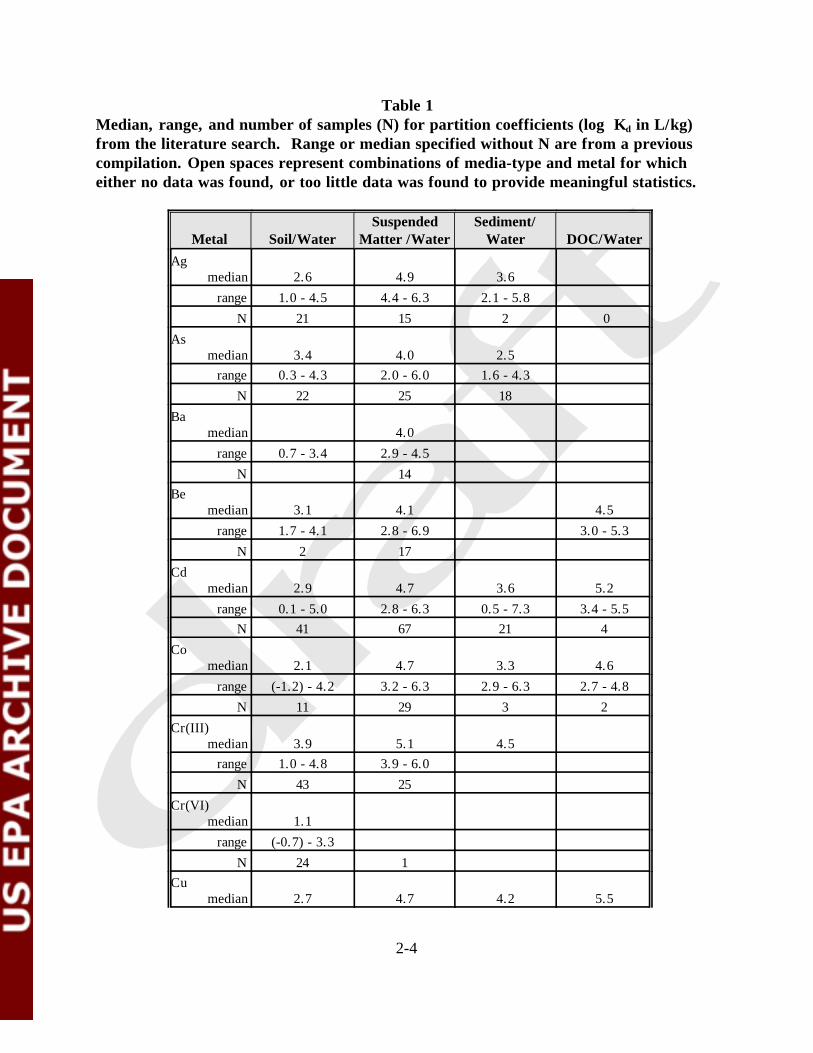
The geochemical parameters most likely to influence the partition coefficient were entered inthe spreadsheet along with reported or calculated coefficients if such were specified in thesource article or report. Examples of these are pH, total concentrations of metal andimportant metal complexing agents including DOC, and weight fraction of particulate organicmatter and other sorbing materials. Physical parameters necessary to convert concentrationratios to partition coefficients in L/kg, including porosity, water content, and bulk densitywere also recorded when reported in the articles. Approximately 245 articles and reports were copied and reviewed. A total of 1170 individualKd values were obtained from these sources directly or calculated from reported mediaconcentrations. This total does not include mean estimated Kd values reported in previouslypublished compilations of Kd values (Baes and Sharp, 1983; Baes et al., 1984; Coughtrey etal., 1985; Thibault et al., 1990). (The data from previous compilations were recorded in thespreadsheet and used in guiding the final estimates of appropriate central tendency values asdescribed in Section 3.1.3.) Approximately 80% of the 1170 values obtained from theliterature pertained to the metals Cd, Co, Cr, Cu, Hg, Ni, Pb, and Zn. More Kd’s wererecovered for Cd than any other metal, followed closely by Zn, Pb, and Cu. The mostfrequently reported type of Kd was that for suspended matter in streams, rivers and lakes. (Data pertaining to marine environments were generally avoided, but some data fromestuaries were included if reported as corresponding to low salinity.) The second mostfrequently reported values pertained to partitioning in soil. Suspended matter and soil Kd’stogether totaled 68% of the reported data. Table 1 below shows the median and range ofliterature Kd values for natural media for each metal and Kd type. (Shown as log Kd values.)
No directly reported partition coefficients for the waste systems of interest were discovered inthe literature survey, and none are included in Table 1. There are many reasons for wishingto understand the behavior of metals in natural systems. The rich literature of soil science,plant nutrition, aquatic chemistry, geology, and toxicology are all examples of investigativeareas of longstanding where metals partition coefficients are frequently encountered. Theimpetus for research with regard to waste systems is significantly different from that ofnatural systems. Moreover, the behavior of metals in waste materials are typically studiedand reported prior to their disposal and consequent mixing with a host of other substances—few studies have focused on the behavior of metals within disposal units containing a (usuallyunknown) mixture of materials. Most studies involving metal concentrations in waste are
2-3
concerned with predicting the metal concentration in leachate by means of a physical test (aleach test). Section 3.2 presents further findings with regard to leach tests and appropriatemetal partition coefficients for waste systems.
2-4
Table 1Median, range, and number of samples (N) for partition coefficients (log Kd in L/kg)from the literature search. Range or median specified without N are from a previouscompilation. Open spaces represent combinations of media-type and metal for whicheither no data was found, or too little data was found to provide meaningful statistics.
Metal Soil/WaterSuspended
Matter /WaterSediment/
Water DOC/WaterAg
median 2.6 4.9 3.6
range 1.0 - 4.5 4.4 - 6.3 2.1 - 5.8
N 21 15 2 0
As median 3.4 4.0 2.5
range 0.3 - 4.3 2.0 - 6.0 1.6 - 4.3
N 22 25 18
Ba median 4.0
range 0.7 - 3.4 2.9 - 4.5
N 14
Be median 3.1 4.1 4.5
range 1.7 - 4.1 2.8 - 6.9 3.0 - 5.3
N 2 17
Cd median 2.9 4.7 3.6 5.2
range 0.1 - 5.0 2.8 - 6.3 0.5 - 7.3 3.4 - 5.5
N 41 67 21 4
Co median 2.1 4.7 3.3 4.6
range (-1.2) - 4.2 3.2 - 6.3 2.9 - 6.3 2.7 - 4.8
N 11 29 3 2
Cr(III) median 3.9 5.1 4.5
range 1.0 - 4.8 3.9 - 6.0
N 43 25
Cr(VI) median 1.1
range (-0.7) - 3.3
N 24 1
Cu median 2.7 4.7 4.2 5.5

Table 1 (continued)Median, range, and number of samples (N) for partition coefficients (log Kd in L/kg) fromthe literature search. Range or median specified without N are from a previouscompilation. Open spaces represent combinations of media-type and metal for which eitherno data was found, or too little data was found to provide meaningful statistics.
Metal Soil/WaterSuspended
Matter /WaterSediment/
Water DOC/Water
2-5
range 0.2 - 3.6 3.1 - 6.1 0.7 - 6.2 2.5 - 7.0
N 20 70 12 17
Hg median 3.8 5.3 4.9
5.4
range 2.2 - 5.8 4.2 - 6.9 3.8 - 6.0 5.3 - 5.6
N 17 35 2 3
CH3Hg median 2.8 5.4 3.9
range 1.3 - 4.8 4.2 - 6.2 2.8 - 5.0
N 11 2 4
Mo median 1.1 2.5
range (-0.2) - 2.7
N 8
Ni median 3.1 4.6 4.0 5.1
range 1.0 - 3.8 3.5 - 5.7 0.4 - 4.7 - 5.4
N 18 30 5 4
Pb median 4.2 5.6 5.1 5.1
range 0.7 - 5.0 3.4 - 6.5 2.0 - 7.0 3.8 - 5.6
N 33 48 24 9
Sb median 2.4 4.0
range 0.1 - 2.7 2.5 - 4.8 2.7 - 4.3
N 6 3
Se median 2.1 4.2 3.6
range -0.3 - 2.4 3.2 - 4.7
N 23 2
Sn median 2.8 5.6 4.7
range 2.1 - 4.0 4.9 - 6.3
N 3

Table 1 (continued)Median, range, and number of samples (N) for partition coefficients (log Kd in L/kg) fromthe literature search. Range or median specified without N are from a previouscompilation. Open spaces represent combinations of media-type and metal for which eitherno data was found, or too little data was found to provide meaningful statistics.
Metal Soil/WaterSuspended
Matter /WaterSediment/
Water DOC/Water
2-6
Tl median
3.2
range 3.0 - 3.5
N 6

Table 1 (continued)Median, range, and number of samples (N) for partition coefficients (log Kd in L/kg) fromthe literature search. Range or median specified without N are from a previouscompilation. Open spaces represent combinations of media-type and metal for which eitherno data was found, or too little data was found to provide meaningful statistics.
Metal Soil/WaterSuspended
Matter /WaterSediment/
Water DOC/Water
2-7
V median
range 0.6 - 2.7
N 1
Zn median 3.1 5.1 3.7 4.9
range (-1.0) - 5.0 3.5 - 6.9 1.5 - 6.2 4.6 - 6.4
N 21 75 18 9
CN median 3.0
range 0.7 - 3.6
N 3
Partition coefficients used in several recent U.S. EPA risk assessments are presented inAppendix A. Because the origin of these data is generally unknown, they were not includedin the collection of Kd values appearing elsewhere in the spreadsheet, nor were they includedin the statistical summary of Kd values obtained from the literature.

3-1
3.0 ANALYSIS OF RETRIEVED DATA AND DEVELOPMENT OFPARTITION COEFFICIENT VALUES
The data gathered from published sources were insufficient to establish a reasonable range forthe partition coefficient for all metals in all media-types. The second part of the effort wasdirected at augmenting the values obtained from the literature so as to provide a reasonablerange and central tendency for each metal in each media-type. Statistical analysis ofretrieved data, geochemical modeling, and expert judgement were all used in developing thepartition coefficients. The nature of the available data for natural media systems and wastesystems was different to the extent that it seemed best to consider these separately.
3.1 DEVELOPMENT OF PARTITIONING COEFFICIENTS IN NATURAL MEDIA
In analyzing the partitioning data collected from the literature for soil and surface watersystems, we attempted to identify the shape of the probability distribution for each metal ineach medium. For a particular metal in a particular medium, the degree to which theliterature sample is truly representative of the population of metal partition coefficients isdependent on the number of sample points, the actual variability of important mediumproperties that influence partitioning (pH, concentration of sorbing phases, etc.), and howwell this variability is represented in the sample. In some cases, it was necessary toeliminate data points from the literature sample to avoid obvious bias. For example, thesample of literature Kd values for Cr(III) in soil included values obtained in a pH titration ofthree soils such that each of the three was represented by 8 different Kd values. Althoughthey provide interesting data on the dependence of Kd on pH in these soils, multiplemeasurements from the same soil and values determined at other than the ambient soil pHintroduce bias in the natural probability distribution of Kd. Therefore, for each of these soils,one of the eight Kd values was picked randomly and the other seven were discarded inderiving the probability distribution. In similar fashion, the sample of literature data for eachmetal and media-type was edited before attempting to identify the underlying distribution.
Statistical tests were performed to determine the shape of the frequency distribution of Kd foreach metal and media-type. The tests employed widely recognized techniques available inthe statistical package Analyze-It (version 1.32), an module add-on for Microsoft EXCEL97. In only a few cases were the data sufficient to identify the underlying distribution withany degree of certainty. Many of the samples, including the most complete samples (largestsample size), gave a positive test for normality after transforming the available data to logspace, suggesting that the frequency distribution of the underlying population of Kd values fora particular metal in a particular medium is most likely log-normal. The Shapiro-Wilk testand the Kolmogorov-Smirnov test were used to test the log transformed samples fornormality. A positive test in Shapiro-Wilk does not ensure a normal distribution. Rather, itprovides a measure of confidence that the sample data are not inconsistent with a normaldistribution. The Shapiro-Wilk test is a general test for normality; it is not necessary toknow the population mean or standard deviation. The Kolmogorov-Smirnov test was usedwhen results from the Shapiro-Wilk test were negative

3-2
In some cases, there were too few representative data points in the sample to have confidencein the descriptive statistics of the data. In these cases, three methods were used to augmentthe available data in estimating the mean, standard deviation, and minimum and maximum Kd
values. The three methods were: estimation from linear regression equations developed fromthe literature samples, estimation from the results of geochemical speciation modeling, andestimation by expert judgement. Each of these is discussed below.
3.1.1 Estimation from Regression Equations Based on Literature Data
Of the 13 metals for which literature data were retrieved characterizing Kd in soil, sediment,and suspended matter, 12 of them exhibited the progression Kd, SPM > Kd,sediment > Kd,soil
(determined by comparison of mean values). In the two other cases where at least two of theKd types could be characterized from the literature data, both conformed to this pattern. Inaddition, consistency was noted in the magnitude of Kd for metals within a specific media. For the best represented metals, the following Kd (affinity) patterns were observed (based onmean Kd):
Soils: Pb > CrIII > Hg > As > Zn = Ni > Cd > Cu > Ag > CoSediment: Pb > Hg > CrIII > Cu > Ni > Zn > Cd > Ag > Co > AsSPM: Pb > Hg > CrIII = Zn > Ag > Cu = Cd = Co > Ni> As There is some shuffling about of the affinity order among these media-types, as might beexpected for a data set that is doubtlessly incomplete. It may be that the As affinity for soilsin our literature sample is too high. Nevertheless, the similarities are worthy of note. Someaspects of the overall trend are in agreement with the hard-soft acid-base (HSAB) concepts ofPearson (1963). Pb and Hg have higher affinity than HSAB predicts. Certainly, there aremultiple adsorbing surfaces present in all of these materials. The consistency of affinityrelationships among these metals suggests that the distribution of Kd is partly due tocharacteristics unique to the metals themselves and partly due to characteristics associatedwith the sorbing surfaces. Regardless of the cause, it appears feasible to exploit theserelationships to provide an estimate of Kd for a metal in one media if its value in anothercould be ascertained. For example, the literature data provided a reasonable number ofsamples of Kd in soils and suspended matter for the nine metals Ag, Cd, Co, Cr(III), Cu, Hg,Ni, Pb, and Zn. For each of these metals, the mean values of Kd in soil was in theneighborhood of two orders of magnitude less than the mean value in suspended matter. Thistrend was characterized more exactly by developing a linear regression equation that wasexploited to estimate mean Kd values for metals for which the literature provided an estimateof mean Kd in soil, but not in suspended matter (or the opposite). In a similar manner, linearregression equations were developed to estimate the mean Kd in sediment from the literatureestimate of mean Kd in soil or suspended matter, or the mean soil Kd from that in sediment orsuspended matter. The regression equations were developed from cases where the literaturesurvey data provided reasonable estimates of the mean Kd for at least two of the three media. The metals used in developing the regression equations included cadmium, copper, zinc, andother metals that were better represented in the literature. The distribution was assumed tobe log-normal so that the regression equations were actually based on mean log Kd and were

3-3
used to predict mean log Kd. The standard deviation was estimated from the mean andminimum values assuming the minimum value represents two standard deviations from themean. It was also estimated in like manner using the mean and maximum values. The largerof the two estimates of standard deviation was retained as the final estimate. The regressionequations used are shown in Table 2 along with the number of observations on which eachequation is based, the correlation coefficient (r2), and the 95% confidence interval for theslope and intercept.
Table 2 Linear Regression Equations used to Estimate Mean log Kd Values (L/kg) in Natural
media.
Used to EstimateDependentVariable
slope( +/- 95% CI)
intercept (+/- 95% CI) r2 N
mean log Kd
sediment mean log Kd
soil1.080
(1.035)0.796
(3.190)0.79 5
mean log Kd
sedimentmean log Kd
suspended matter1.418
(1.923)-3.179(9.868)
0.65 5
mean log Kd
suspended mattermean log Kd
soil0.380
(0.444)3.889
(1.338)0.37 9
mean log Kd
suspended mattermean log Kd
sediment0.457
(0.619)3.257
(2.555)0.65 5
mean log Kd
soilmean log Kd
sediment0.728
(0.697)0.071
(2.878)0.79 5
mean log Kd
soilmean log Kd
suspended matter0.969
(1.136)-1.903(5.703)
0.37 9
The regressions equations were also used to estimate mean Kd values for suspended matterand sediments from an estimate of the mean Kd in soil obtained from geochemical speciationmodeling.
3.1.2 Estimation From Geochemical Speciation Modeling
Geochemical speciation modeling was used to estimate soil/water partitioning if regressionequations could not be used. The partitioning of metal cations between DOC and theinorganic portion of the solution phase was also estimated by speciation modeling. In bothcases, the U.S. EPA geochemical speciation model MINTEQA2 version 4.0 (Allison et al.,1990) was used to estimate the Kd values. The input data for MINTEQA2 was developedfrom various sources.
Modeling details for soil partition coefficients

3-4
The concentrations of major ions were the average concentrations in river water as reportedby Stumm and Morgan (1996). The soil water phosphate concentration was obtained fromBohn et al. (1979). The ionic strength was held constant at 0.005 M after a sensitivity test inthe range 0.01 to 0.001 M revealed that the impact was significantly less than other importantvariables. Model values for several of the most significant variables affecting Kd were variedover reasonable ranges in order to capture the expected range in Kd. These master variablesinclude pH, concentration of dissolved organic carbon (DOC), concentration of particulateorganic carbon (POC), and concentration of metal oxide binding sites. The range for each ofthese was characterized by low, medium, and high values, and the model was executed at allpossible combinations of these settings. The pH range corresponded to that reported from theSTORET database (U.S. EPA, 1996a) with a slight downward adjustment (6.5 for themedium value instead of 6.8, and 4.5 for the low value instead of 4.9) to account for themore acidic environment of surface watershed soils. The concentrations used for DOC were0.5, 5.0, and 50.0 mg/L, taken as a reasonable range in soil water. The POC concentrationswere obtained from analysis of shallow silt-loam soils from a soils database (Carsel et al.,1988 and R. Parrish, personal communication). The low, medium, and high values were ascorresponds to the 10th, 50th, and 90th percentiles, respectively, for particulate organic matter(0.41, 1.07, and 2.12 wt%).
The dominant metal oxide sorbing surface was assumed to be hydrous ferric oxide (HFO). Because we had little reliable information as to the appropriate concentration range, and alsoin consideration of the importance of this variable in determining Kd, the HFO concentrationwas used as a calibrating variable. The low, medium, and high values were first set tocorrespond to the values used in U.S. EPA (1996a). Those values were based on aspecialized extraction of reactive Fe from a set of 12 samples from aquifers and soils. Themean Kd for Cd, Cu, Ni, Pb, and Zn were computed using these values in MINTEQA2. These were compared with mean Kd values for these metals in soil from the literature survey. The low, medium, and high HFO concentrations were scaled in subsequent modeling suchthat the mean Kd value from MINTEQA2 was within the 95% confidence interval of the meanliterature Kd value for each of these metals. (Each MINTEQA2 execution resulted in 81different Kd values due to utilizing all different combinations of low, medium, and high forthe four different master variables. The mean value from MINTEQA2 was taken as theaverage of the three Kd values corresponding to the medium setting of pH, DOC, and HFOand the low POC; the medium settings of pH, DOC, and HFO, and the medium POC; and themedium settings of pH, DOC, and HFO, and the high setting of POC.) Appendix B shows atypical MINTEQA2 input file used in estimating Kd for soil/water.
The minimum and maximum Kd values were established from the available literature data andthe MINTEQA2 results. The distribution was assumed to be log-normal. Once the mean logKd value for a metal was established for soil from the modeling exercise, the regressionequations were used to estimate mean values for sediment and suspended matter if these werelacking in the literature data. The standard deviation was estimated as described above forlinear regression estimates.
Modeling details for DOC partition coefficients

3-5
(1)
(2)
The partitioning of metals between DOC and other inorganic forms in water is not usuallyreported in terms of a partitioning coefficient. In fact, specialized algorithms withinspeciation models are frequently employed to estimate the fraction of metal bound with DOCbased on the pH, major ion composition of the solution, and ionic strength. The developmentof such specialized methods for estimating metal binding with DOC is an ongoing researcharea. MINTEQA2 includes a specialized sub-model for estimating DOC interactions—theGaussian distribution model (Dobbs et al., 1989; Allison and Perdue, 1994). This modelrepresents DOC as a mixture of many types of metal binding sites. The probability ofoccurrence of a binding site with a particular log K is given by a normal probability functiondefined by a mean log K and standard deviation in log K. A limitation of the DOC bindingcalculations in MINTEQA2 and similar models is that the metal-DOC reactions necessary toobtain results are available only for a limited number of metal cations and for none of theanionic metals. MINTEQA2 includes mean log K values for the metal cations Cd, Cu, Ba,Be, Cr(III), Ni, Pb, and Zn. For other metal cations of interest (Ag, Co, Hg(II), Sn(II), andTl(I)) it was necessary to estimate the mean log K for DOC binding for use with the Gaussianmodel. For Hg(II), the estimate of the mean log K was determined from a regression of“known” mean log K values with the binding constants for humic- and fulvic acid (HA andFA, respectively) as given by Tipping (1994). The metals Cd, Cu, Ni, Pb, and Zn wererepresented in the database of HA and FA binding constants, so these were used to developthe regression relationship:
This relationship was derived with a correlation coefficient (r2) of 0.95. It was used toestimate a mean log KDOC,Hg of 9.0 for Hg+2 binding with DOC.
The mean log K for the other cations (Ag+, Co2+, Sn2+, and Tl+) were derived from a linearfree energy relationship using the first hydrolysis constants (log KOH) and the bindingconstant for acetate (log KAcet). The log KOH and log KAcet for the metals Cd, Cu, Fe, Ni, Pb,and Zn were used to derive the following relationship:
The correlation coefficient (r2) for this relationship is 0.98. It was used to estimate the meanlog KDOC for Ag+, Co2+, Sn2+, and Tl+ for use in MINTEQA2 modeling. The mean logKDOC values estimated for these metals were 2.0, 3.3, 6.6, and 1.0, respectively.
The estimation procedures outlined above cannot reliably be extended to anions. However,anions are typically not as strongly bound to organic matter. We therefore have used
3-6
MINTEQA2 to estimate Kd values with DOC for cationic metals only and have includedconservative estimates for the anions based on judgement alone.
The concentrations of major ions used in estimating metal-DOC binding using MINTEQA2were the average concentrations in river water as reported by Stumm and Morgan (1996). The concentration of DOC and the pH were treated as master variables with each assignedthree levels corresponding to low, medium, and high. The medium value was the mean of thereported river and stream samples from the literature survey, and the low and high valueswere selected to encompass the range observed in the literature survey data. Specifically, thelow, medium, and high DOC were 0.89, 8.9, and 89 mg/L, respectively, and the lowmedium, and high pH were 4.9, 7.3, and 8.1, respectively. The binding of each of the metalcations was computed in nine simulations that represented all possible combinations of pHand DOC concentration level. The mean value Kd value for the cations was represented bythe value computed by MINTEQA2 when the pH and DOC concentration were set to theirmean values in surface water. A typical MINTEQA2 input file used to estimate metalpartitioning with DOC is shown in Appendix C.
The results computed using MINTEQA2 for both soils and DOC were used to augment thepartitioning data collected in the literature survey. Although it was considered reasonable touse MINTEQA2 to estimate mean partition coefficients, it is not possible to establish theshape of the distribution from the MINTEQA2 results. However, there is no compellingreason to suppose other than the log-normal distribution suggested by the literature surveydata.
3.1.3 Estimation from Expert Judgement
When neither the regression equations nor MINTEQA2 could reasonably be used to estimatethe mean log Kd, the mean value was estimated subjectively using expert judgement. Factorsconsidered included any values obtained from the literature survey, reported mean values orranges from precious compilations, similarities of behavior among metals, and qualitativestatements from articles and reports. The minimum and maximum Kd values from theliterature were used if reasonable values were available. Otherwise, these were alsoestimated by expert judgement. In either case, the standard deviation was estimated asdescribed above for linear regression.
Finally, a relative confidence level (CL) was subjectively assigned to each of the final valuespresented. The CL values range from 1 to 4 with the highest confidence corresponding to avalue of 1, and the lowest to a value of 4. In general, estimates based on the literaturesurvey for a well-studied metal with a large literature sample was deemed to merit a CL of 1. Data for a metal not represented in the literature for which the final values were purelyestimates from MINTEQA2 or other means with a notable degree of expert judgement wereassigned a CL of 4. Many data were determined in circumstances that warrant a CL betweenthese extremes (e.g., a range was given in the literature, a value was available from aprevious compilation, estimates from combinations of these circumstances could be combined

3-7
with estimates from modeling, etc.). In these cases, a CL of 2 or 3 was assigned as seemedbest.
The metal partition coefficients in soil, sediment, suspended matter, and DOC are presentedin Tables 3, 4, 5, and 6, respectively. The method used to arrive at each estimate isindicated for each metal and media-type, as is the subjectively assigned confidence level.

Table 3 Metal partition coefficients (log Kd) in kg/L for soil/soil water. Values in italics were estimated by regression or fromMINTEQA2 results. An entry of “log-normal” in bold indicates that the sample data gave a positive result in theShapiro-Wilk test for normality of the log-transformed data. An entry of “log-normal” in parentheses means that datawere not sufficient to establish the distribution, but log-normal has been assumed. Relative confidence in the data isindicated by the CL value of 1 to 4 (1=highest, 4=lowest).
MetalDistribution(assumed) Median Mean Std. Dev. Min Max Comments
Ag (I) Log Normal 2.6 2.6 0.8 1.0 4.5 From literature data (raw, n=21); CL=1
Asa (log-normal) 3.4 3.2 0.7 0.3 4.3 From literature data (raw, n=21); oxidation stateusually not specified in literature; CL=2
Ba(II) (log-normal) --- 2.0 0.7 0.7 3.4 Suspended matter Kd regression equation for mean;CL=2
Be(II) (log-normal) --- 2.2 1.0 1.7 4.1 Suspended matter Kd regression equation for mean;CL=3
Cd(II) Log Normal 2.9 2.7 0.8 0.1 5.0 From literature data (edited, n=37); CL=1
Co(II) Log Normal 2.1 2.1 1.2 -1.2 4.1 From literature data (raw, n=11); CL=1
Cr(III) Log Normal 3.9 3.8 0.4 1.0 4.7 From literature data (raw, n=22); CL=2
Cr(VI) (log-normal) 1.1 0.8 0.8 -0.7 3.3 From literature data (raw, n=24); CL=2
Cu(II) Log Normal 2.7 2.5 0.6 0.1 3.6 From literature data (raw, n=20); CL=1
Hg(II) Log Normal 3.8 3.6 0.7 2.2 5.8 From literature data (raw, n=17); CL=1
MeHg Log Normal 2.8 2.7 0.6 1.3 4.8 From literature data (raw, n=11); CL=2
Mo(VI) (log-normal) 1.1 1.3 0.6 -0.4 2.7 From literature data (raw, n=5); oxidation state notalways specified in literature data; CL=3
Ni(II) Log Normal 3.1 2.9 0.5 1.0 3.8 From literature data (raw, n=19); CL=1

Table 3 (continued) Metal partition coefficients (log Kd) in kg/L for soil/soil water. Values in italics were estimated by regression or fromMINTEQA2 results. An entry of “log-normal” in bold indicates that the sample data gave a positive result in the Shapiro-Wilk test for normality of the log-transformed data. An entry of “log-normal” in parentheses means that data were notsufficient to establish the distribution, but log-normal has been assumed. Relative confidence in the data is indicated by theCL value of 1 to 4 (1=highest, 4=lowest).
MetalDistribution(assumed) Median Mean Std. Dev. Min Max Comments
Pb(II) (log-normal) 4.1 3.7 1.2 0.7 5.0 From literature data (edited, n=31); CL=2
Sbb (log-normal) --- 2.3 1.1 0.1 2.7 From literature data (mean is the average of severalreported mean values, n=5); CL=4
Se(IV)c (log-normal) 1.4 1.3 0.4 -0.3 2.4 From literature data (edited, n=11); CL=2
Se(VI) (log-normal) --- -0.2 1.1 -2.0 2.0 Mean estimated from MINTEQA2 result; min, maxare guesses; CL=4
Sn(II) (log-normal) --- 2.7 0.7 2.1 4.0 From literature data, CL=3
Tl(I) (log-normal) --- 0.5 0.9 -1.2 1.5 Estimated from MINTEQA2 result. CL=4
V(V) (log-normal) --- 1.7 1.5 0.5 2.5 Mean, min, max from suspended matter Kd
regression equation; CL=4
Zn(II) (log-normal) 3.1 2.7 1.0 -1.0 5.0 From literature data (raw, n=21); CL=1
CN- (log-normal) --- 0.7 1.6 -2.4 1.3 Estimated from MINTEQA2 result. CL=4
a Published partitioning data for As does not allow differentiation of As(III) and As(V). It is probable that published values representresults involving both oxidation states.
b Published partitioning data for Sb is rare and does not allow differentiation of Sb(III) and Sb(V).c Positive result in Shapiro-Wilk test for normality of data not log-transformed. But sample size is small and data may not be very
representative.

Table 4 Metal partition coefficients (log Kd) in kg/L for sediment/porewater. Values in italics were estimated by regression orfrom MINTEQA2 results. An entry of “log-normal” in bold indicates that the sample data gave a positive result in theShapiro-Wilk test for normality of the log-transformed data. An entry of “log-normal” in parentheses means that datawere not sufficient to establish the distribution, but log-normal has been assumed. Relative confidence in the data isindicated by the CL value of 1 to 4 (1=highest, 4= lowest).
MetalDistribution(assumed) Median Mean Std. Dev. Min Max Comments
Ag(I) (log-normal) --- 3.6 1.1 2.1 5.8 Mean from soil Kd regression equation; min, maxfrom literature data; CL=3
Asa Log-normal 2.2 2.4 0.7 1.6 4.3 From literature data; Oxidation state not specified inliterature data; CL=2
Ba(II) (log-normal) --- 2.5 0.8 0.9 3.2 Mean, min, max from suspended matter Kd regressionequation; CL=3
Be(II) (log-normal) --- 2.8 1.9 0.8 6.5 Mean, min, max from suspended matter Kd regressionequation; CL=3
Cd(II) Log-normal 3.7 3.3 1.8 0.5 7.3 From literature data (n=14, edited); CL=1
Co(II) (log-normal) --- 3.1 1.0 2.9 3.6 Mean from soil Kd regression equation; min, maxfrom literature data; CL=3
Cr(III) (log-normal) --- 4.9 1.5 1.9 5.9 Mean, min, max from soil Kd regression equation;CL=4
Cr(VI) (log-normal) --- 1.7 1.4 0.0 4.4 Mean, min, max from soil Kd regression equation;CL=4
Cu(II) Log-normal 4.1 3.5 1.7 0.7 6.2 From literature data (raw, n = 12); CL=1
Hg(II) (log-normal) --- 4.9 0.6 3.8 6.0 From literature data (raw, n=2); CL=2
MeHg (log-normal) --- 3.9 0.5 2.8 5.0 From literature data (edited, n=2), CL=2
Mo(VI) (log-normal) --- 2.5 0.8 0.4 3.7 Mean from literature data (reported mean value withoxidation state not specified); min, max from soil Kd
regression equation; CL=4

Table 4 (continued) Metal partition coefficients (log Kd) in kg/L for sediment/porewater. Values in italics were estimated by regression or fromMINTEQA2 results. An entry of “log-normal” in bold indicates that the sample data gave a positive result in the Shapiro-Wilk test for normality of the log-transformed data. An entry of “log-normal” in parentheses means that data were notsufficient to establish the distribution, but log-normal has been assumed. Relative confidence in the data is indicated by theCL value of 1 to 4 (1=highest, 4= lowest).
MetalDistribution(assumed) Median Mean Std. Dev. Min Max Comments
Ni(II) (log-normal) --- 3.9 1.8 0.3 4.0 Mean from soil Kd regression equation; min, maxfrom literature data; CL=3
Pb(II) Log-normal 5.1 4.6 1.9 2.0 7.0 From literature data (edited, n=14); CL=1
Sbb (log-normal) --- 3.6 1.8 0.6 4.8 From literature data (reported mean value); CL=4
Se(IV) (log-normal) --- 3.6 1.2 1.0 4.0 Mean from literature data (reported mean value);min, max are guesses; CL=4
Se(VI) (log-normal) --- 0.6 1.2 -1.4 3.0 Mean, min, max from soil Kd regression equation;CL=4
Sn(II) (log-normal) --- 3.7 0.7 3.1 5.1 Mean, min, max from soil Kd regression equation;CL=3
Tl(I) (log-normal) --- 1.3 1.1 -0.5 3.5 Mean, min from soil Kd regression equation; maxfrom literature data; CL=4
V(V) (log-normal) --- 2.1 0.9 0.4 3.2 Mean, min, max from suspended matter Kd regressionequation; CL=4
Zn(II) (log-normal) 4.8 4.1 1.6 1.5 6.2 From literature data (edited, n=13); CL=1
CN- (log-normal) --- 1.6 1.7 -1.8 2.2 Mean, min, max from soil Kd regression equation;CL=4
a Published metal partitioning data does not allow differentiation of As(III) and As(V). It is probable that the data presented includeresults for both oxidation states.
b Published partitioning data for Sb is rare and does not allow differentiation of Sb(III) and Sb(V).
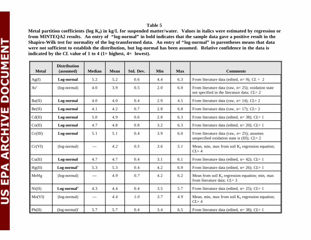
Table 5 Metal partition coefficients (log Kd) in kg/L for suspended matter/water. Values in italics were estimated by regression orfrom MINTEQA2 results. An entry of “log-normal” in bold indicates that the sample data gave a positive result in theShapiro-Wilk test for normality of the log-transformed data. An entry of “log-normal” in parentheses means that datawere not sufficient to establish the distribution, but log-normal has been assumed. Relative confidence in the data isindicated by the CL value of 1 to 4 (1=highest, 4= lowest).
MetalDistribution(assumed) Median Mean Std. Dev. Min Max Comments
Ag(I) Log-normal 5.2 5.2 0.6 4.4 6.3 From literature data (edited, n=9); CL = 2
Asa (log-normal) 4.0 3.9 0.5 2.0 6.0 From literature data (raw, n=25); oxidation statenot specified in the literature data; CL=2
Ba(II) Log-normal 4.0 4.0 0.4 2.9 4.5 From literature data (raw, n=14); CL=2
Be(II) Log-normal 4.1 4.2 0.7 2.8 6.8 From literature data (raw, n=17); CL=2
Cd(II) Log-normal 5.0 4.9 0.6 2.8 6.3 From literature data (edited, n=38); CL=1
Co(II) Log-normal 4.7 4.8 0.8 3.2 6.3 From literature data (edited, n=20); CL=1
Cr(III) Log-normal 5.1 5.1 0.4 3.9 6.0 From literature data (raw, n=25); assumesunspecified oxidation state is (III); CL=2
Cr(VI) (log-normal) --- 4.2 0.5 3.6 5.1 Mean, min, max from soil Kd regression equation;CL=4
Cu(II) Log-normal 4.7 4.7 0.4 3.1 6.1 From literature data (edited, n=42); CL=1
Hg(II) Log-normalb 5.3 5.3 0.4 4.2 6.9 From literature data (edited, n=26); CL=1
MeHg (log-normal) --- 4.9 0.7 4.2 6.2 Mean from soil Kd regression equation; min, maxfrom literature data; CL=3
Ni(II) Log-normalb 4.3 4.4 0.4 3.5 5.7 From literature data (edited, n=25); CL=1
Mo(VI) (log-normal) --- 4.4 1.0 3.7 4.9 Mean, min, max from soil Kd regression equation;CL=4
Pb(II) (log-normal)c 5.7 5.7 0.4 3.4 6.5 From literature data (edited, n=38); CL=1

Table 5 (continued) Metal partition coefficients (log Kd) in kg/L for suspended matter/water. Values in italics were estimated by regression orfrom MINTEQA2 results. An entry of “log-normal” in bold indicates that the sample data gave a positive result in theShapiro-Wilk test for normality of the log-transformed data. An entry of “log-normal” in parentheses means that datawere not sufficient to establish the distribution, but log-normal has been assumed. Relative confidence in the data isindicated by the CL value of 1 to 4 (1=highest, 4= lowest).
MetalDistribution(assumed) Median Mean Std. Dev. Min Max Comments
Sbd (log-normal) --- 4.8 0.5 3.9 4.9 Mean, min, max from soil Kd regression equation;CL=4
Se(IV) (log-normal) --- 4.4 0.4 3.8 4.8 Mean, min, max from soil Kd regression equation;CL=4
Se(VI) (log-normal) --- 3.8 1.0 3.1 4.6 Mean, min, max from soil Kd regression equation;CL=4
Sn(II) (log-normal) --- 4.9 0.8 4.7 6.3 Mean, min from soil Kd regression equation; maxfrom literature data; CL=4
Tl(I) (log-normal) --- 4.1 1.0 3.0 4.5 Mean from soil Kd regression equation; otherparameters are guesses; CL=4
V(V) (log-normal) --- 3.7 0.6 2.5 4.5 Mean from literature data (raw, n=5); min, max areguesses; oxidation state not always specified inliterature; CL=3
Zn(II) Log-normal 5.1 5.0 0.5 3.5 6.9 From literature data (edited, n=47); CL=1
CN- (log-normal) --- 4.2 0.6 3.0 4.4 Mean, min, max from soil Kd regression equation;CL=4
a Positive result for Shapiro-Wilk test for normality of data not log-transformed. But published metal partitioning data does not allowdifferentiation of As(III) and As(V). It is probable that the data represented include results for both oxidation states.
b Failed Shapiro-Wilk test for normality of log-transformed data, but passed the Kolmogorov-Smirnov test and histogram exhibits log-normal character
c Failed Shapiro-Wilk and the Kolmogorov-Smirnov test for normality of log-transformed data, but histogram exhibits log-normal characterd Published partitioning data for Sb is rare and does not allow differentiation of Sb(III) and Sb(V).

Table 6 Metal partition coefficients (log Kd) in kg/L for partitioning between DOC and inorganic solution species. Values in italicswere estimated by regression or from MINTEQA2 results. Log-normal distributions are assumed. Relative confidence inthe data is indicated by the CL value of 1 to 4 (1=highest, 4=lowest).
MetalDistribution(assumed) Mean Std. Dev. Min Max Comment
A g(I) (log-normal) 2.5 1.0 1.5 4.5 Mean estimated from MINTEQA2 results;other parameters are guesses; CL = 3
As (log-normal) 2.0 1.0 0.0 3.0 No data, values are conservative guesses; CL=4
Ba(II) (log-normal) 3.6 1.0 2.5 4.0 Mean estimated from MINTEQA2 results, values for otherparameters are guesses; CL=3
Be(II) (log-normal) 2.1 1.0 1.1 3.8 All parameters estimated from MINTEQA2 results; CL=3
Cd(II) (log-normal) 3.8 0.9 2.0 5.5 Mean estimated from MINTEQA2 results; min, max areguesses; CL=3
Co(II) (log-normal) 3.8 0.9 2.0 5.5 Mean estimated from MINTEQA2 results; min, max areguesses; CL=3
Cr(III) (log-normal) 1.1 1.6 -0.6 4.3 Mean estimated from MINTEQA2 results; min, max areguesses; CL=4
Cr(VI) (log-normal) 2.0 1.0 0.0 3.0 No data, values are conservative guesses; CL=4
Cu(II) (log-normal) 5.4 1.1 2.5 7.0 From literature data (raw, n=17); CL=2
Hg(II) (log-normal) 5.4 1.2 3.0 6.0 Mean from literature data (raw, n=3); min, max are guesses;CL=4
MeHg (log-normal) 5.0 1.1 2.8 5.5 Mean, min, max estimated based on relative Kd’s of Hg(II)and MeHg for suspended matter and Hg(II) Kd with DOC.
Ni(II) (log-normal) 3.7 0.9 1.9 5.4 Mean estimated from MINTEQA2 results; min, max areguesses; CL=3
Mo(VI) (log-normal) 2.0 1.0 0.0 3.0 No data, values are conservative guesses; CL=4
Pb(II) (log-normal) 4.9 0.5 3.8 5.6 From literature data (raw, n=9); CL=2

Table 6 (continued)Metal partition coefficients (log Kd) in kg/L for partitioning between DOC and inorganic solution species. Values in italicswere estimated by regression or from MINTEQA2 results. Log-normal distributions are assumed. Relative confidence inthe data is indicated by the CL value of 1 to 4 (1=highest, 4=lowest).
MetalDistribution(assumed) Mean Std. Dev. Min Max Comment
Sb (log-normal) 2.0 1.0 0.0 3.0 No data, values are conservative guesses; CL=4
Se(IV) (log-normal) 2.0 1.0 0.0 3.0 No data, values are conservative guesses; CL=4
Se(VI) (log-normal) 2.0 1.0 0.0 3.0 No data, values are conservative guesses; CL=4
Sn(II) (log-normal) 2.0 1.0 0.0 3.0 No data, values are conservative guesses; CL=4
Tl(I) (log-normal) 1.6 1.0 0.0 3.0 Mean estimated from MINTEQA2, values for otherparameters are guesses; CL=4
V(V) (log-normal) 2.0 1.0 0.0 3.0 No data, values are conservative guesses; CL=4
Zn(II) (log-normal) 5.1 0.7 4.6 6.4 From literature data (raw, n=9); CL=3
CN- (log-normal) 2.0 1.0 0.0 3.0 No data, values are conservative guesses; CL=4

3-16 HydroGeoLogic, Inc 11/16/99
3.2 DEVELOPMENT OF PARTITIONING COEFFICIENTS FOR WASTE SYSTEMS
The multimedia, multi-pathway risk assessment for HWIR utilizes a source model thatassumes equilibrium partitioning in land application units (LAUs), waste piles, landfills,treatment lagoons (surface impoundments), and aerated tanks. The available data forcharacterizing the partitioning of metals in waste consists almost exclusively of leach testresults for specific wastes. The literature search did not produce any study that specificallyprovides measured partitioning coefficients for metals in the mixed materials present in wastemanagement units.
Several studies have addressed the issue of the applicability of leach test data in predictingthe leachate concentration from landfills (U.S. EPA, 1991). The U.S. EPA ToxicityCharacteristic Leaching Procedure (TCLP) was specifically designed to predict leachateconcentrations for wastes co-disposed with municipal solid waste. Recent papers present theidea that the concentration observed in any leach test depends a great deal on leaching timeand the cumulative solid-liquid ratio (van der Sloot et al., 1996). Three “regimes” arerecognized in the leaching process (de Groot and van der Sloot, 1992): 1) leachingconcentration controlled by initial wash-off of loosely adhered contaminant, 2) leachingconcentration controlled by dissolution of primary materials and perhaps re-precipitation ofmore stable phases, and 3) leaching concentration controlled by the diffusion of wasteconstituent from the interior of waste particles to the particle surface. The time of onset andduration of these regimes is highly variable and is interrelated with the life-cycle of the wastesystem (acetogenesis, methanogenesis, etc.). The chemical composition (major ionconcentration and concentration of metal-complexing organic ligands) is also important indetermining the leaching concentration that will be observed in any particular case. Ingeneral, it would seem that the highest concentrations are expected during the initial wash-offperiod, with concentrations declining thereafter. An immediately obvious question is: Whatperiod is of concern in the modeling for the HWIR rulemaking? Since, the model does notallow a time-variable partition coefficient, it would seem that an aggregate partitioncoefficient that represents an average over time would be desired. Unfortunately, there iscurrently no way to know whether the “partitioning” observed in a TCLP test corresponds tosuch an average value. Most authors seem to regard the TCLP as an aggressive test that mayoverestimate metal concentrations. However, there is no consensus on this point.
In view of the lack of data describing partitioning of metals in different types of waste units,the following simplifications are proposed:
1) For land application units, the partition coefficients for soils presented in Table 3 shouldbe used. This simplification assumes that the partitioning behavior of metals in an LAUis likely to be dominated by the sorptive characteristics of the soil underlying the unit.
2) For surface impoundments and aerated tanks, the partition coefficients for suspendedmatter presented in Table 5 should be used. This seems a reasonable step in thatpartitioning in such systems must involve sorption to suspended particles and sediments. The composition and quantity of suspended and sedimented sorbing particles must bequite variable, but there is no source of data on which to base modeling or otherestimating techniques.

3-17 HydroGeoLogic, Inc 11/16/99
3) Waste piles and landfills should be treated the same as regards metal partitioning.
Adopting these simplifications, it is necessary to derive estimates of metal partitioncoefficients for waste piles and landfills only. The sections below detail how these have beenestimated from available TCLP and similar leach tests that present both solid phase andcorresponding leachate concentrations. We have used statistical methods and geochemicalspeciation modeling to extend results to metals not represented in reported TCLP or otherleach test results and to examine the similarity between expected waste partitioning andpartitioning in natural media.
3.2.1 Estimation from Analysis of Data Presented in the Literature
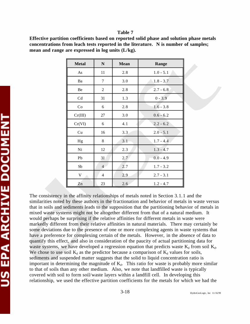
There are numerous papers and journal articles describing results from a TCLP or similarleach test for a particular waste. These published studies often focus on waste constituentleachability before and after a waste stabilization or treatment process. There are manypublished studies of leachability of metals from incinerator ash with the aim of investigatingthe suitability of the ash materials for disposal or for use in construction. Frequently, leachtest results (leachate concentrations) are reported without the corresponding concentration inthe solid phase. This omission makes those data useless in estimating expected partitioning. The literature survey produced 203 leach test results for which both leachate and solid phasedata are presented. Table 7 shows the range and mean values of effective partitioncoefficients for each metal for which sufficient data was found. We refer to these aseffective partition coefficients because they are simply the ratio of metal in the solid andsolution phases as represented in the leach test results. They may or may not representequilibrium partitioning.
Several authors discussed the similarities in metal leachability over a range of differentmaterials. A study by van der Sloot et al. (1996) examined the leaching behavior of Cd andZn from various ash materials, shredded municipal solid waste, sewage sludge-amended soil,and soil. Similar characteristics were noted in pH dependent leaching of both Cd and Znfrom the nine different materials studied. Differences among the different materials wereattributed to waste-specific chemical parameters that caused a different chemical speciation. The authors gave an example of Cd complexation with chloride which they investigated usingMINTEQA2. The increased leachability of Cd in some of the ash materials was correlatedwith chloride concentration in the waste.
Flyhammar (1997) concluded that there are similarities in the metal binding properties ofmunicipal solid waste (MSW) and sediments. He found that the fractionation of metalsamong various available and reactive forms (as determined by sequential chemicalextractions) was similar between fresh MSW and an oxic sediment. Similarities were alsofound in the fractionation patterns of aged MSW and anoxic sediments.
3-18 HydroGeoLogic, Inc 11/16/99
Table 7Effective partition coefficients based on reported solid phase and solution phase metalsconcentrations from leach tests reported in the literature. N is number of samples;mean and range are expressed in log units (L/kg).
Metal N Mean Range
As 11 2.8 1.0 - 5.1
Ba 7 3.0 1.8 - 3.7
Be 2 2.8 2.7 - 6.8
Cd 31 1.3 0 - 3.9
Co 6 2.8 1.6 - 3.8
Cr(III) 27 3.0 0.6 - 6.2
Cr(VI) 6 4.1 2.2 - 6.2
Cu 16 3.3 2.0 - 5.1
Hg 8 3.1 1.7 - 4.4
Ni 12 2.3 1.3 - 4.7
Pb 31 2.7 0.0 - 4.9
Sb 4 2.7 1.7 - 3.2
V 4 2.9 2.7 - 3.1
Zn 23 2.6 1.2 - 4.7
The consistency in the affinity relationships of metals noted in Section 3.1.1 and thesimilarities noted by these authors in the fractionation and behavior of metals in waste versusthat in soils and sediments leads to the supposition that the partitioning behavior of metals inmixed waste systems might not be altogether different from that of a natural medium. Itwould perhaps be surprising if the relative affinities for different metals in waste weremarkedly different from their relative affinities in natural materials. There may certainly besome deviations due to the presence of one or more complexing agents in waste systems thathave a preference for complexing certain of the metals. However, in the absence of data toquantify this effect, and also in consideration of the paucity of actual partitioning data forwaste systems, we have developed a regression equation that predicts waste Kd from soil Kd. We chose to use soil Kd as the predictor because a comparison of Kd values for soils,sediments and suspended matter suggests that the solid to liquid concentration ratio isimportant in determining the magnitude of Kd. This ratio for waste is probably more similarto that of soils than any other medium. Also, we note that landfilled waste is typicallycovered with soil to form soil/waste layers within a landfill cell. In developing thisrelationship, we used the effective partition coefficients for the metals for which we had the

3-19 HydroGeoLogic, Inc 11/16/99
most complete (largest) sample. The regression equation thus determined is log Kd,waste = 0.7log Kd,soil + 0.3. The relationship has a correlation coefficient of (r2) of 0.4 implying that40% of the variation in log Kd,waste from the leach test data is predicted.
3.2.2 Estimation from Geochemical Speciation Modeling
The MINTEQA2 geochemical speciation model was used to investigate the range of metalpartitioning coefficients for landfills. The input requirements of the model for estimatingmetal partitioning include the concentrations of major ions, the pH, the concentrations ofsorbing phases, and the DOC concentration. Four landfill modeling scenarios weredeveloped, distinguished primarily by the concentrations of major ions, the DOCconcentration, the POC concentration, and the pH. The scenarios included landfillscontaining municipal solid waste in the acetogenic stage and in the methanogenic stage, amonofill containing ash from incineration of municipal solid waste (MSWI ash), and amonofill containing cement kiln dust (CKD).
For each of the MINTEQA2 modeling scenarios, a hydrous ferric oxide sorbing phase wasassumed. A particulate organic carbon sorbent was also assumed for the acetogenic andmethanogenic MSW landfills. Particulate organic carbon was assumed to have been consumedin the incineration process for the MSWI and CKD scenarios. The concentration of thesorbent is crucial in determining the number of sites available for metal sorption. Unfortunately, the concentration of sorbent appropriate in waste systems is subject to a veryhigh degree of uncertainty. The uncertainty arises from the variable composition of wastesthat are disposed in landfills and the possible changes in composition over time as leachatepercolates through the materials. It is not unlikely that surfaces exposed to landfill gas andleachate undergo changes with respect to their sorptive character over time. Possible changesinclude dissolution or precipitation of oxide or organic surface coatings. These processeshave not been studied in actual landfill samples in sufficient detail to allow quantitativerepresentation. Kersten et al. (1997) cited evidence of sorption control of Pb leaching inMSWI leach tests. They attempted to model the observed Pb concentrations by utilizing aspeciation model with surface complexation sorption reactions parameterized for the constantcapacitance model assuming hydrous ferric oxide as the sorbent. They obtained reasonableresults assuming 0.7 g/L for the HFO concentration and using a site density of 1.35x10⁻⁴ molsites/g HFO. The MINTEQA2 modeling presented here utilized a similar surfacecomplexation model (the diffuse-layer model). Kersten et al. (1997) had noted that theirsorbent concentration was perhaps too low, so the modeling was conducted both with theirvalue of 0.7 g/L, and using 7 g/L as a reasonable upper-range value. In both cases, a sitedensity 1.35x10⁻⁴ mol sites/g HFO was used.
The values of other parameters and constituent concentrations used in the modeling for thefour scenarios are shown in Table 8. After concentration of sorbing sites, the most criticalmodel parameter is pH, so the modeling was conducted at three different pH values for eachscenario. The three pH values used for the acetogenic and methanogenic scenarios (4.5, 6.1,7.5 and 7.5, 8.0, 9.0, respectively) were in keeping with the minimum, maximum and meanpH cited for these landfill stages in a study of 15 landfills by Ehrig (1992). The major ion

3-20 HydroGeoLogic, Inc 11/16/99
concentrations for the acetogenic and methanogenic scenarios were also as specified in Ehrig(1992). The three pH values for the MSWI scenario (8.0, 9.0, 10.0) were selected to define areasonable range and central tendency value for this scenario. These values were based ondata collected in the literature review portion of this study, as were the major ionconcentrations for the MSWI scenario. The pH values associated with the CKD scenariowere selected with due consideration to the highly alkaline conditions associated with thismaterial, but they lack statistical significance. An example MINTEQA2 input file for eachof the scenarios is presented in Appendix D.
It should be noted that the confidence level associated with all of the modeling parameters forwaste systems is low. There is not an extensive database of observations from which toextract reasonable model values for most of these parameters, especially the concentration ofsorbents and sorbing sites. Without reliable information for characterizing the sorbents, it isnot possible to accurately establish the total system concentrations of competing ions (Ca,Mg, etc.) that should be used in the model. The results must be interpreted in light of thisshortcoming.

3-21 HydroGeoLogic, Inc 11/16/99
Table 8 Important parameters and constituent concentrations used in MINTEQA2 modeling oflandfills in the acetogenic and methanogenic stages and MSWI and CKD monofills.
ModelParameter
Scenario
MSWAcetogenic
MSWMethanogenic
MSWIAsh Monofill
CKDMonofill
pH 4.5, 6.1, 7.5a 7.5, 8.0, 9.0a 8.0, 9.0, 10.0b 9.0, 10.0, 11.0c
Ca 6000d 975d 1,700b 2850f
Mg 625d 500d 10b 10f
Na 1350e 1350e 300b 300f
K 1100e 1100e 380b 400f
CO3 500c 250c 50c 50f
Cl 2100e 2100e 1,200b 380f
Fe 780e --- --- ---
SO4 500d 80d 1,400b 630f
IonicStrength (M)
0.1c 0.1c 0.1c 0.1c
DOC 100c 50c 15c 15c
POC 100,000c 50,000c --- ---
a Minimum, average, and maximum values reported in Ehrig (1992)b Obtained from analysis of data MSWI obtained in literature surveyc Reasonable guessesd Computed from typical dissolved values reported in Ehrig (1992) and assumingequilibrium with the model sorbents at the median pH for acetogenic and methanogeniccases. e Reported as typical values in Ehrig (1992)f Generated from simulation of TCLP on CKD using MINTEQA2 (U.S. EPA, 1998b)
The partitioning coefficients estimated from the MINTEQA2 modeling exercise for severalmetals are shown in Table 9. The values presented were converted to units of L/kg byassuming that one liter of leachate solution is associated with 5 kg of waste material. Therange in estimated partition coefficients is shown for each scenario. In interpreting theseresults, it must be remembered that no statistical significance can be assigned because nonecan be associated with most of the model input parameters. At best, these results should be

3-22 HydroGeoLogic, Inc 11/16/99
regarded as indicating a possible range of central tendency values, and even this must bequalified because the results are so sensitive to several poorly characterized parameters, mostnotably, the concentration of sorbents. The results also reflect only a single concentrationvalue for each of the major ions— variability in these concentrations will influence metalpartitioning. Some ions exert greater influence on the partitioning of particular metals. Forexample, the low partition coefficients associated with Cd appear to be related tocomplexation with chloride, which is entered at high concentrations in all scenarios. Thiseffect is in keeping with observations by others (van der Sloot et al., 1996). Another majorion whose concentration level may influence metal partitioning is calcium. At the highconcentrations of these ions in waste systems, especially MSWI ash and CKD, thecompetition for binding sites can become very important with regard to trace metal binding. For those metals whose partitioning is significantly influenced by the concentration level of amajor ion, it is expected that this fact would contribute to a broader range of observedpartition coefficients in real systems than that calculated in this modeling exercise.
Table 9Estimated range in log partition coefficients (L/kg) for selected metals determined from
MINTEQA2 modeling.
Metal
Estimated log Kd (L/kg)
MSWAcetogenesis
MSWMethanogenesis
MSWIAsh Monofill
CKDMonofill
Be 0.8 - 3.9 3.3 - 4.4 (-0.4) - 4.0 ---
Cd (-0.3) - 0.0 0.6 - 1.7 (-1.0) - 1.1 (-0.4) - 1.2
Co 0.2 - 0.3 0.9 - 1.8 (-0.9) - 0.4 (-2.0) - 0.2
Cr(III) 1.1 - 3.5 3.8 - 4.8 (-0.2) - 3.2 ---
Cu 1.1 - 1.9 2.0 - 2.5 0.0 - 2.9 (-2.0) - 2.1
Ni 0.2 - 0.4 1.1 - 1.9 (-0.04) - 1.1 (- 1.5) - 0.9
Pb 1.7 - 2.7 3.3 - 4.2 2.4 - 3.6 0.7 - 3.4
Zn 0.4 - 0.7 1.5 - 2.1 (-0.6) - 1.3 ---
In comparing the partition coefficients estimated using MINTEQA2 with those for soils,there is greater agreement with values predicted by the derived regression equation (logKd,waste = 0.7 log Kd,soil + 0.3; see Section 3.2.1) for some metals than for others. (Themeasure of “agreement” for a metal is whether the value predicted by the equation using themean soil Kd value of Table 3 falls within the range of MINTEQA2 estimates for that metal. Using this rather lax requirement for agreement, the modeled Kd values for Be, Cr(III), Cu,and Pb agree, those of Cd and Ni do not agree, and those of Co and Zn are marginal.) Likethe literature-reported Kd values for natural media, Pb and Cr(III) tend to have high Kd
3-23 HydroGeoLogic, Inc 11/16/99
estimates from MINTEQA2 . In general, the results for the acetogenic and methanogeniclandfill scenarios agree more closely with the regression relationship with soil Kd values thando the more alkaline cases for ash and CKD. It is probable that the lower Kd values in thelatter are due to the combination of high major ion concentrations that compete for sorbingsites and solubilize the metals by complexation, and the absence of particulate organic carbonin the model systems.
In view of the uncertainties inherent in the model results, a possible alternative forrepresenting metal partitioning in waste piles and landfills is to use the regression equationpresented in Section 3.2.1. This has the advantage of preserving the relative affinities amongmetals that has been noted as common to the natural media. However, the model results dosuggest that the Kd values in alkaline systems may be significantly lower than in municipallandfills. This might be accounted for by treating the slope and intercept coefficients in theregression as variables subject to uncertainty that can be represented in the monte carloiterations. In the overall modeling strategy of HWIR, if the frequency of occurrence of ahighly alkaline waste system can be established and used in the monte carlo realizations, thecoefficients could be adjusted to give lower Kd values for the appropriate fraction ofrealizations to reflect alkaline systems. This topic needs further study, as does the entireissue of equilibrium partitioning in waste. It should be noted that of the several studiesreviewed whose authors suggested mechanisms controlling the leachate concentrations ofmetals, most advocated a mineral solubility control rather than equilibrium partitioning(Bäverman et al., 1997; Kersten et al., 1997; Johnson et al., 1996; Eighmy et al., 1995; Yanand Neretnieks, 1995; Fruchter et al., 1990; Moretti et al, 1988; Gould et al., 1988). However, the difficulty in distinguishing solubility controls from effects of sorption is alsonoted. It is possible that metals are initially mobilized by dissolution of solid phases,especially in ash and CKD, but that surface coatings that form upon aging eventually controlsolution phase metal concentrations via sorption (van der Sloot et al., 1996). More researchis need to quantify these processes in waste systems.

4-1 HydroGeoLogic, Inc 11/16/99
4.0 REFERENCES
The reference list includes the complete bibliography of papers, articles, and reports thatwere copied and reviewed in the literature search. Those articles which provided data forspreadsheet entry are identified by a code in square brackets at the end of the citation. Thecode can be cross-referenced to spreadsheet entries. Further explanation of spreadsheetentries is provided in the spreadsheet itself.
Abdel-Moati, M. A. R., 1998. Speciation of selenium in a Nile Delta lagoon and SEMediterranean Sea mixing zone. Estuarine, Coastal and Shelf Science, 46:621-628.
Albino, V., R. Cioffi, L. Santoro, and G. L. Valenti, 1996. Stabilization of residuecontaining heavy metals by means of matrices generating calcium trisulphoaluminateand silicate hydrates. Waste Management & Research, 14:29-41. [Al96]
Allen, H. E., Y. Chen, Y. Li, C. P. Huang, and P. F. Sanders, 1995. Soil partitioncoefficients by column desorption and comparison to batch adsorption measurements. Environmental Science & Technology, 29(8):1887-1891. [Al95]
Allison, J.D., D.S. Brown, and K.J. Novo-Gradac, 1990. MINTEQA2/PRODEFA2, AGeochemical Assessment Model for Environmental Systems: Version 3.0 User'sManual. U.S. Environmental Protection Agency, Athens, GA. EPA/600/3-91/021.
Allison, J.D. and E.M. Perdue, 1994. Modeling metal-humic interactions with MINTEQA2,in Humic Substances in the Global Environment and Implications on Human Health,edited by N. Senesi and T.M. Miano, Elsevier Science B.V.
Amdurer, M., 1983. Chemical Speciation and Cycling of Trace Elements in Estuaries:Radiotracer Studies in Marine Microcosms. Ph.D. Dissertation, ColumbiaUniversity, 475 p. [Am83]
Anderson, M. A., R. K. Ham, R. Stegman, and R. Stanforth, 1979. Test factors affectingthe release of materials from industrial wastes in leaching tests. Toxic and HazardousWaste Disposal, Volume 2: Options for Stabilization/Solidification, R. B. Pojasek,ed., Ann Arbor Science, Ann Arbor, Michigan, p. 145-168. [An79]
Anderson, P. R. and T. H. Christensen, 1988. Distribution coefficients of Cd, Co, Ni, andZn in soils. Journal of Soil Science, 39:15-22. [An88]
Andres, A. and J. A. Irabien, 1994. Solidification/stabilization process for steel foundrydust using cement based binders: influence of processing variables. WasteManagement & Research, 12:405-415. [An94]

4-2 HydroGeoLogic, Inc 11/16/99
Angelidis, M. and R. J. Gibbs, 1989. Chemistry of metals in anaerobically treated sludges. Water Research, 23(1):29-33.
Avezzù, F., G. Billolotti, C. Collivignarelli, and A. V. Ghirardini, 1995. Behaviour ofheavy metals in activated sludge biological treatment of landfill leachate. WasteManagement & Research, 13:103-121. [Av95]
Baes, III, C. F. and R. D. Sharp, 1983. A proposal for estimation of soil leaching andleaching constants for use in assessment models. Journal of Environmental Quality,12(1):17-28. [Ba83]
Baes, III, C. F., R. D. Sharp, A. L. Sjoreen, and R. W. Shor, 1984. A Review and Analysisof Parameters for Assessing Transport of Environmentally Released RadionuclidesThrough Agriculture. U. S. Department of Energy, Oak Ridge National Laboratory,ONRL-5786, 150 p.
Balls, P. W., 1989. The partition of trace metals between dissolved and particulate phases inEuropean coastal waters: a compilation of field data and comparison with laboratorystudies. Netherlands Journal of Sea Research, 23(1):7-14. [Ba89a]
Bangash, M. A. and J. Hanif, 1992. Sorption behavior of cobalt on illitic soil. WasteManagement, 12:29-38. [Ba92]
Barkay, T., M. Gillman, and R. R. Turner, 1997. Effects of dissolved organic carbon andsalinity on bioavailability of mercury. Applied and Environmental Microbiology,63:4267-4271.
Barna, R., P.Moszkowicz, J. Veron, and M. Tirnoveanu, 1994. Solubility model for thepore solution of leached concrete containing solidified waste. Journal of HazardousMaterials, 37:33-39. [Ba94]
Baskaran, M., M. Ravichandran, and T. S. Bianchi, 1997. Cycling of 7Be and 210Pb in ahigh DOC, shallow, turbid estuary of southeast Texas. Estuarine, Coastal and ShelfScience, 45:165-176. [Ba97]
Bäverman, C., A. Sapiej, L. Moreno, and I. Neretnieks, 1997. Serial batch tests performedon municipal solid waste incineration bottom ash and electric arc furnace slag, incombination with computer modelling. Waste Management & Research, 15:55-71.[Ba97b]
Beaublen, S., J. Nrlagu, D. Blowes, and G. Lawson, 1994. Chromium speciation in thegreat lakes. Environmental Science & Technology, 28:730-738. [Be94b]

4-3 HydroGeoLogic, Inc 11/16/99
Becker, U. and S. Peiffer, 1997. Heavy-metal ion complexation by particulate matter in theleachate of solid waste: a multi-method approach. Journal of Contaminant Hydrology,24:313-344. [Be97]
Behel, Jr., D., D. W. Nelson, and L. E. Sommers, 1983. Assessment of heavy metalequilibria in sewage sludge-treated soil. Journal of Environmental Quality,12(2):181-186.
Belevi, H., D. and P. Baccini, 1989. Long-term behaviour of municipal solid wastelandfills. Waste Management & Research, 7:43-56. [Be89]
Belevi, H., D. M. Stampfli, and P.Baccini, 1992. Chemical behaviour of municipal solidwaste incinerator bottom ash in monofills. Waste Management & Research, 10:153-167. [Be92b]
Benedetti, M. F., W. H. van Riemsdijk, L. K. Koopal, D. G. Kinniburgh, D. C. Gooddy,and C. J. Milne, 1996. Metal ion binding by natural organic matter: From the modelto the field. Geochimica et Cosmochimica Acta, 60(14):2503-2513.
Benoit, G., 1995. Evidence of the particle concentration effect for lead and other metals infresh waters based on ultraclean technique analyses. Geochimica et CosmochimicaActa, 59(13):2677-2687. [Be95]
Benoit, G., S. D. Oktay-Marshall, A. Cantu, II, E. M. Hood, C. H. Coleman, M. O.Corapcioglu, and P. H. Santschi, 1994. Partitioning of Cu, Pb, Ag, Zn, Fe, Al, andMn between filter-retained particles, colloids, and solution in six Texas estuaries. Marine Chemistry, 45:307-336. [Be94]
Bhat, P. N. and K. C. Pillai, 1997. Leachability and immobilisation of beryllium from solidwaste (red-mud) generated in processing beryl. Water, Air, and Soil Pollution,94:297-306. [Bh97]
Bishop, P. L., 1988. Leaching of inorganic hazardous constituents from stabilized/solidifiedhazardous wastes. Hazardous Waste & Hazardous Materials, 5(2):129-143. [Bi88]
Breault, R. F., J. A. Colman, G. R. Aiken, and D. McKnight, 1996. Copper speciation andbinding by organic matter in copper-contaminated streamwater. EnvironmentalScience & Technology, 30(12):3477-3486. [Br96]
Bohn, H. L., B. L. McNeal, and G. A. O’Connor, 1979. Soil Chemistry, Wiley-Interscience, John Wiley and Sons, New York.
Brannon, J. M. and W. H. Patrick, Jr., 1987. Fixation, transformation, and mobilization ofarsenic in sediments. Environmental Science & Technology, 21(5):450-459. [Br87]

4-4 HydroGeoLogic, Inc 11/16/99
Bunde, R. L., J. J. Rosentreter, and M. J. Liszewski, 1998. Rate of strontium sorption andthe effects of variable aqueous concentrations of sodium and potassium on strontiumdistribution coefficients of a surficial sediment at the Idaho National EngineeringLaboratory, Idaho. Environmental Geology, 34(2/3):135-142.
Carsel, R.F., R. S. Parrish, R. L. Jones, J. L. Hansen, and R. L. Lamb, 1988. Characterizing the uncertainty of pesticide leaching in agricultural soils. Journal ofContaminant Hydrology, 2: 111-124.
Cabanis, S. E. and M. S. Shuman, 1988. Copper binding by dissolved organic matter: I. Suwannee River fulvic acid equilibria. Geochimica et Cosmochimica, 52:185-193.
Cabanis, S. E. and M. S. Shuman, 1988. Copper binding by dissolved organic matter: II. Variation in type and source of organic matter. Geochimica et Cosmochimica,52:195-200.
Campbell, D. J. and P. H. T. Beckett, 1988. The soil solution in a soil treated with digestedsewage sludge. Journal of Soil Science, 39:283-298. [Ca88c]
Cernuschi, S., M. Giugliano, and I. de Paoli, 1990. Leaching of residues from MSWincineration. Waste Management & Research, 8:419-427. [Ce90]
Chang, C., 1993. Toxicity of Sediment-Bound Thallium to Marine Organisms. Ph.D.Dissertation, University of Washington, 163 p. [Ch93b]
Cheeseman, C. R., E. J. Butcher, C. J. Sollars, and R. Perry, 1993. Heavy metal leachingfrom hydroxide, sulphide, and silicate stabilised/solidified wastes. WasteManagement, 13(8):545-552. [Ch93c]
Cheng, K. Y. and P. L. Bishop, 1992. Sorption, important in stabilized/solidified wasteforms. Hazardous Waste & Hazardous Materials, 9(3):289-296. [Ch92c]
Cheng, K. Y. and P. Bishop, 1992. Metals distribution in solidified/stabilized waste formsafter leaching. Hazardous Waste & Hazardous Materials, 9(2):163-171.
Chichester, D. L. and S. Landsberger, 1996. Determination of the leaching dynamics ofmetals from municipal solid waste incinerator fly ash using a column test. Journal ofthe Air & Waste Management Association, 46:643-649. [Ch96c]
Chiffoleau, J., D. Cossa, D. Aufer, and I. Truquet, 1994. Trace metal distribution,partition and fluxes in the Seine estuary (France) in low discharge regime. MarineChemistry, 47:145-158.

4-5 HydroGeoLogic, Inc 11/16/99
Christensen, T. H., 1985. Cadmium sorption at low concentrations. IV. Effect of wasteleachates on distribution coefficients. Water, Air, and Soil Pollution, 26:265-274.[Ch85]
Christensen, T. H., F. Bertelsen, and G. Gissel-Nielsen, 1989. Selenite fixation by soilparticle-size separates. Journal of Soil Science, 40:641-647. [Ch89]
Coker, E. G. and P. J. Matthews, 1983. Metals in sewage sludge and their potential effectsin agriculture. Water Science Technology, 15:209-225.
Comber, S. D. W., A. M. Gunn, and C. Whalley, 1995. Comparison of the partitioning oftrace metals in the Humber and Mersey estuaries. Marine Pollution Bulletin, pp.851-860. [Co95]
Cornett, J., L. Chant, and B. Risto, 1992. Arsenic transport between water and sediments. Hydrobiologia, 235/236:533-544. [Co92a]
Cote, P. L. and D. Isabel, 1984. Application of a dynamic leaching test to solidifiedhazardous wastes. Hazardous and Industrial Waste Management and Testing: ThirdSymposium, ASTM STP 851, L. P. Jackson, A. R. Rohlik, and R. A. Conway, Eds.,American Society for Testing and Materials, Philadelphia, pp. 193-212. [Co84]
Coughtrey, P. J., D. Jackson, and M. C. Thorne, 1985. Radionuclide Distribution andTransport in Terrestrial and Aquatic Ecosystems: A Compendium of Data; Volume Six. A. A. Balkema, Rotterdam and Boston. [Co85]
Cutter, G. A., 1989. The estuarine behavior of selenium in San Francisco Bay. Estuarine,Coastal and Shelf Science, 28:13-34. [Cu89]
Davis, A. and J. N. Galloway, 1993. Distribution of Pb between sediments and pore waterin Woods Lake, Adirondack State Park, New York, U.S.A. Applied Geochemistry,8:51-65. [Da93]
de Groot, G. J. and H. A. van der Sloot, 1992. Determination of leaching characteristics ofwaste materials leading to environmental certification. Stabilization and Solidificationof Hazardous, Radioactive, and Mixed Wastes, 2nd Volume, ASTM STP 1123, T. M.Gilliam and C. C. Wiles, Eds., American Society for Testing and Materials,Philadelphia, 1992, pp.149-170. [Gr92]
Del Castilho, P. and W. J. Chardon, 1995. Uptake of soil cadmium by three soil crops andits prediction by a pH-dependent Freundlich sorption model. Plant and Soil, 171:263-266.

4-6 HydroGeoLogic, Inc 11/16/99
Deverel, S. J. and S. P. Millard, 1988. Distribution and mobility of selenium and othertrace elements in shallow groundwater of the western San Joaquin Valley, California. Environmental Science & Technology, 22(6):697-702.
Dobbs, J. C., W. Susetyo, L. A. Carreira, and L. V. Azarraga, 1989. Competitive bindingof protons and metals ions in humic substances by lanthanide ion probe spectroscopy. Analytical Chemistry, 61:1519-1524.
Dusing, D. C., P. L. Bishop, and T. C. Keener, 1992. Effect of redox potential on leachingfrom stabilized/solidified waste materials. Journal of the Air & Waste ManagementAssociation, 42:56-62. [Du92]
Dzombak, D.A. and F.M.M. Morel, 1990. Surface Complexation Modeling: Hydrous FerricOxide, John Wiley and Sons, New York.
Earle, C. D. A., 1997. The Fate of Mercury in Municipal Solid Waste Landfills and ItsPotential for Volatilization. Ph.D. Dissertation, University of Florida, 261 p.
Eckert, Jr., J. O. and Q. Guo, 1998. Heavy metals in cement and cement kiln dust fromkilns co-fired with hazardous waste-derived fuel: application of EPA leaching andacid-digestion procedures. Journal of Hazardous Materials, 59:55-93. [Ec98]
Egemen, E. and C. Yuteri, 1996. Regulatory leaching tests for fly ash: a case study. WasteManagement & Research, 14:43-50. [Eg96b]
Ehrig, H., 1992. Leachate quality. In: Landfilling of Waste: Leachate, T. H. Christensen,R. Cossu, and R. Stegmann, eds., Elsevier Applied Science, London and New York,520 p. [Eh92]
Eighmy, T. T., J. D. Eusden, Jr., J. E. Krzanowski, D. S. Domingo, D. Stämpfli, J. R.Martin, and P. M. Erickson, 1995. Comprehensive approach toward understandingelement speciation and leaching behavior in municipal solid waste incinerationelectrostatic precipitator ash. Environmental Science & Technology, 29(3):629-646.[Ei95]
Elbaz-Poulichet, F., J. Garnier, D. M. Guan, J. Martin, and A. J. Thomas, 1996. Theconservative behavior of trace metals (Cd, Cu, Ni and Pb) and As in the surfaceplume of stratified estuaries: example of the Rhone River (France). Estuarine,Coastal and Shelf Science, 42:289-310. [El96]
Faust, B. C., 1992. The octanol/water distribution coefficients of methylmercuric species:the role of aqueous-phase chemical speciation. Environmental Toxicology andChemistry, 11:1373-1376.

4-7 HydroGeoLogic, Inc 11/16/99
Faye, M. S. and M. L. Diamond, 1996. The role of phytoplankton in the removal of arsenicby sedimentation from surface waters. Hydrobiologia, 324:117-123. [Fa96]
Fernandez-Sempere, J., M. L. Barrueso-Martinez, R. Font-Montesinos, and M. C. Sabater-Lillo, 1997. Characterization of tannery waste — Comparison of three leachabilitytests. Journal of Hazardous Materials, 54:31-45. [Fe97]
Fio, J. L., R. Fujii, and S.J. Deverel, 1991. Selenium mobility and distribution in irrigatedand non-irrigated alluvial soils. Soil Science Society of America Journal, 55:1313-1320. [Fi91]
Fisher, S., 1979. The problems of developing consensus on methodology for predicting theleaching characteristics of deposited waste. Toxic and Hazardous Waste Disposal,Volume 2: Options for Stabilization/Solidification, R. B. Pojasek, ed., Ann ArborScience, Ann Arbor, Michigan, p. 169-187. [Fi79]
Fletcher, P. and P. H. T. Beckett, 1987. The chemistry of heavy metals in digested sewage sludge — I. Copper(II) complexation with soluble organic matter. Water Research,21(10):1153-1161. [Fl87]
Flyhammar, P., 1997. Estimation of heavy metal transformations in municipal solid waste. The Science of the Total Environment, 198:123-133.
Flyhammar, P., F. Tamaddon, and L. Bengtsson, 1998. Heavy metals in a municipal solidwaste disposal cell. Waste Management and Research, 16(5):403-410. [Fl98]
Fotovat, A. and R. Naidu, 1997. Ion exchange resin and MINTEQA2 speciation of Zn andCu in alkaline sodic and acidic soil extracts. Australian Journal of Soil Research,35:711-726.
Fruchter, J. S., D. Rai, and J. M. Zachara, 1990. Identification of solubility controllingsolid phases in a large fly ash field lysimeter. Environmental Science & Technology,24:1173-1179.
Gagnon, C. and N. S. Fisher, 1997. Bioavailability of sediment-bound methyl and inorganicmercury to a marine bivalve. Environmental Science & Technology, 31(4):993-998.
Gambrell, R. P. and W. H. Patrick, Jr., 1989. Cu, Zn, and Cd availability in a sludge-amended soil under controlled pH and redox potential conditions. In: EcologicalStudies, Volume 74, B. Bar-Yosef, J. Goldschmid, and N. J. Barrow, eds., Springer-Verlag, New York, 200 p. [Ga89]
Gao, S., W. J. Walker, R. A. Dahlgren, and J. Bold, 1997. Simultaneous sorption of Cd,Cu, Ni, Zn, Pb, and Cr on soils treated with sewage sluge supernatant. Water, Air,and Soil Pollution, 93: 331-345.[Ga97b]
4-8 HydroGeoLogic, Inc 11/16/99
Garnier, J. -M., J. -M. Martin, J. -M. Mouchel, and K. Sioud, 1996. Partitioning of tracemetals between the dissolved and particulate phases and particulate surface reactivityin the Lena River estuary and the Laptev Sea (Russia). Marine Chemistry, 53:269-283. [Ga96]
Garnier, J. -M., M. K. Pham, P. Ciffroy, and J. -M. Martin, 1997. Kinetics of traceelement complexation with suspended matter and with filterable ligands in freshwater. Environmental Science & Technology, 31(6):1597-1606. [Ga97a]
Gavasci, R., F. Lombardi, A. Polettini, and P. Sirini, 1998. Leaching tests on solidifiedproducts. Journal of Solid Waste Technology and Management, 25(1):14-20. [Ga98]
Gerritse, R. G., R. Vriesema, J. W. Dalenberg, and H. P. De Roos, 1982. Effect of sewagesludge on trace element mobility in soils. Journal of Environmental Quality, 11:359-364. [Ge82]
Gooddy, D. C., P. Shand, D. G. Kinniburgh, and W. H. van Riemsdijk, 1995. Field-basedpartition coefficients for trace elements in soil solutions. European Journal of SoilScience, 46:265-285. [Go95b]
Gould, J. P., F. G. Pohland, and W. H. Cross, 1988. Mobilization and retention of mercuryand lead from particulates co-disposed with municipal solid wastes. ParticulateScience and Technology, 6:381-392. [Go88]
Gounaris, V., P. R. Anderson, and T. M. Holsen, 1993. Characteristics and environmentalsignificance of colloids in landfill leachate. Environmental Science & Technology,27(7):1381-1387.
Goyette, M. L. and B. -A. G. Lewis, 1995. Kd in screening-level ground-water contaminant-transport model. Journal of Environmental Engineering, 121(7):537-541.
Graham, E. R., 1973. Selective distribution and labile pools of micronutrient elements asfactors affecting plant uptake. Soil Science of America Proceedings, 37:70-74.
Grimanis, A. P., M. Vassilaki-Grimani, and N. Kalogeropoulos, 1994. Pollution studies ofsilver and antimony in Saronikos Gulf, Greece by INAA. Journal of Radioanalyticaland Nuclear Chemistry, Articles, 179(2):231-241.
Guo, R., C. L. Chakrabarti, K. S. Subramanian, X. Ma, Y. Lu, J. Cheng, and W. F.Pickering, 1993. Sorption of low levels of cyanide by granular activated carbon. Water Environment Research, 65:640-644.

4-9 HydroGeoLogic, Inc 11/16/99
Hall, W. S., K. L. Dickson, F. Y. Saleh, J. H. Rodgers, Jr., D. Wilcox, and A. Entazami,1986. Effects of suspended solids on the acute toxicity of zinc due to daphnia magnaand pimephales promelas. Water Resources Bulletin, 22(6):913-920.
Hassan, S. M. and A. W. Garrison, 1996. Distribution of chromium species between soiland porewater. Chemical Speciation and Bioavailability, 8(3/4):85-103. [Ha96b]
Hassan, S. M., A. W. Garrison, H. E. Allen, D. M. Di Toro, and G. T. Ankley, 1996. Estimation of partition coefficients for five trace metals in sandy sediments andapplication to sediment quality criteria. Environmental Toxicology and Chemistry,15(12):2198-2208. [Ha96a]
Hawley, N., J. A. Robbins, and B. J. Eadie, 1986. The partitioning of beryllium in freshwater. Geochimica et Cosmochimica Acta, 50:1127-1131. [Ha86b]
Henke, K. R., B. J. Zobeck, C. J. Moretti, and M. D. Mann, 1987. Leaching studies ofsolid wastes generated from fluidized bed combustion of low-rank western coals. Proceedings of the 1987 International Conference on Fluidized Bed Combustion,pp.954-959. [He87]
Hering, J. G. and F. M. M. Morel, 1988. Humic acid complexation of calcium and copper. Environmental Science & Technology, 22(10):1234-1237.
Hemming, C. H., R. L. Bunde, M. J. Liszewski, J. J. Rosentreter, and J. Whelan, 1997. Effect of experimental technique on the determination of strontium distributioncoefficients of a surficial sediment from the Idaho National Engineering Laboratory,Idaho. Water Research, 31(7):1629-1636.
Herrera, Jr., E., M. Tittlebaum, F. Cartledge, and H. Eaton, 1992. Evaluation of theleaching properties of solidified heavy metal wastes. Journal of EnvironmentalScience and Health, Part A, 27(4):983-998.
Herut, B. and Kress, N., 1997. Particulate metals contamination in the Kishon Riverestuary, Israel. Marine Pollution Bulletin, 34(9):706-711.
Hiraide, M., S. Hiramatsu, and H. Kawaguchi, 1994. Evaluation of humic complexes oftrace metals in river water by adsorption on indium-treated XAD-2 resin and DEAE-Sephadex A-25 anion exchanger. Fresenius Journal of Analytical Chemistry, 348:758-761. [Hi94]
Hooper, K., M. Iskander, G. Sivia, F. Hussein, J. Hsu, M. Deguzman, Z. Odion, Z. Ilejay,F. Sy, M. Petreas, and B. Simmons, 1998. Toxicity characteristic leaching procedurefails to extract oxoanion-forming elements that are extracted by municipal solid wasteleachates. Environmental Science & Technology, 32:3825-3830. [Ho98]

4-10 HydroGeoLogic, Inc 11/16/99
Hue, N. V. and S. A. Ranjith, 1994. Sewage sludges in Hawaii: Chemical composition andreactions with soils and plants. Water, Air, and Soil Pollution, 72:265-283.
Hurley, J. P., M. M. Schafer, S. E. Cowell, J. T. Overdier, P. E. Hughes, and D. E.Armstrong, 1996. Trace metal assessment of Lake Michigan tributaries using low-level techniques. Environmental Science & Technology, 30(6):2093-2098. [Hu96]
Ishak, C. F., 1993. Characterization and Trace Contaminant Chemistry of Coal CombustionBy-Products. Ph.D. Dissertation, University of Georgia, Athens, Georgia. [Is93]
Jackson, D. R., B. C. Garret, and T. A. Bishop, 1984. Comparison of batch and columnmethods for assessing leachability of hazardous waste. Environmental Science &Technology, 18(9):668-673. [Ja84]
Janssen, R. P. T., W. J. G. M. Peijnenburg, L. Posthuma, and M. A. G. T. van Den Hoop,1997. Equilibrium partitioning of heavy metals in Dutch field soils. I. Relationshipbetween metal partition coefficients and soil characteristics. EnvironmentalToxicology and Chemistry, 16(12):2470-2478. [Ja97]
Johnson, C. A., L. Sigg, and U. Lindauer, 1992. The chromium cycle in a seasonallyanoxic lake. Limnology and Oceanography, 37(2):315-321.
Johnson, C. A., M. Kersten, F. Ziegler, and H. C. Moor, 1996. Leaching behaviour andsolubility— controlling solid phases of heavy metals in municipal solid wasteincinerator ash. Waste Management, 16:129-134. [Jo96]
Johnson, W. H., S. M. Serkiz, and S. B. Clark, 1994. Determination of site specificdistribution coefficients of mixed waste contaminants using an in-situ approach. Proceedings of the 27th Mid-Year Meeting of the Health Physics Society: ManagingMixed and Radioactive Waste, Albany, New York, February 13-17, 1994. [Jo94b]
Jones, K. C., B. E. Davies, and P. J. Peterson, 1986. Silver in Welsh soils: Physical andchemical distribution studies. Geoderma, 37:157-174. [Jo86]
Jones, L. W., R. M. Bricka, and M. J. Cullinane, Jr., 1992. Effects of selected wasteconstituents on solidified/stabilized waste leachability. Stabilization andSolidification of Hazardous, Radioactive, and Mixed Wastes, 2nd Volume, ASTMSTP 1123, T. M. Gilliam and C. C. Wiles, Eds., American Society for Testing andMaterials, Philadelphia, 1992, pp. 193-203. [Jo92b]
Jopony, M. and S. D. Young, 1994. The solid— solution equilibria of lead and cadmium inpoluted soils. European Journal of Soil Science, 45:59-70.

4-11 HydroGeoLogic, Inc 11/16/99
Joshi, S. R. and B. S. Shukla, 1991. The role of the water/soil distribution coefficient in thewatershed transport of environmental radionuclides. Earth and Planetary ScienceLetters, 105:314-318. [Jo91]
Jin, X., G. W. Bailey, Y. S. Yu, and A. T. Lynch, 1996. Kinetics of single and multiplemetal ion sorption processes on humic substances. Soil Science, 161(8):509-520.[Ba96]
Kaminski, M. D., 1998. Assessment of Gross Accumulation and Leaching Characteristics ofHeavy Metals in a Contaminated Urban Soil. Ph.D. Dissertation, University ofIllinois at Urbana-Champaign, 216 p.
Karuppiah, M. and G. Gupta, 1997. Toxicity of and metals in coal combustion ash leachate. Journal of Hazardous Materials, 56:53-58.
Kersten, M., H. C. Moor, and C. A. Johnson, 1997. Speciation of trace metals in leachatefrom a MSWI bottom ash landfill. Applied Geochemistry, 12:675-683.
Kida, A., Y. Noma, and T. Imada, 1996. Chemical speciation and leaching properties ofelements in municipal incinerator ashes. Waste Management, 16(5/6):527-536.[Ki96b]
Kiratli, N. and M. Ergin, 1996. Partitioning of heavy metals in surface Black Seasediments, 1996. Applied Geochemistry, 11:775-788.
Koelmans, A. A., F. Gillissen, and L. Lijklema, 1996. Influence of salinity andmineralization on trace metal sorption to cyanobacteria in natural waters. WaterResearch, 30(4):853-864.
Koelmans, A. A. and L. Luklema, 1992. Sorption of 1,2,3,4-tetrachlorobenzene andcadmium to sediments and suspended solids in Lake Volkerak/Zoom. WaterResearch, 26(3):327-337. [Ko92]
Korzun, E. A. and H. H. Heck, 1990. Sources and fates of lead and cadmium in municipalsolid waste. Journal of the Air Waste Management Association, 40(9):1220-1226.
Kuo, S. and E. J. Jellum, 1991. Affinity and behavior of Cd sorption in some acid soils. Water, Air, and Soil Pollution, 57-58:369-376. [Ku91]
Lagas, P., C. M. Bom, M. J. t’ Hart, H. A. M. de Kruijf, and J. P. G. Loch, 1981. Modelexperiments on the behaviour of cyanide and barium in a landfill and in the soil. Studies in Environmental Science, W. van Duijvenbooden, P. Glasbergen, and H. vanLelyveld, Eds. 17:539-543.

4-12 HydroGeoLogic, Inc 11/16/99
Lake, D. L., P. W. W. Kirk, and J. N. Lester, 1984. Fractionation, characterization, andspeciation of heavy metals in sewage sludge and sludge-amended soils: A review. Journal of Environmental Quality, 13(2):175-183.
Lamy, I., S. Bourgeois, and A. Bermond, 1993. Soil cadmium mobility as a consequence ofsewage sludge disposal. Journal of Environmental Quality, 22:731-737.
Lecuyer, I., S. Bicocchi, P. Ausset, and R. Lefevre, 1996. Physico-chemicalcharacterization and leaching of desulphurization coal fly ash. Waste Managementand Research, 14:15-28. [Le96b]
Lee, C. -H., H. -C. Wang, C. -M. Lin, and G. C. C. Yang, 1994. A long-term leachabilitystudy of solidified wastes by the multiple toxicity characteristic leaching procedure. Journal of Hazardous Materials, 38:65-74. [Le94b]
Lee, P. -L., P. Baillif, and J. -C. Touray, 1997. Geochemical behaviour and relativemobility of metals (Mn, Cd, Zn, and Pb) in recent sediments of a retention pond alongthe A-71 motorway in Sologne, France. Environmental Geology, 32(2):142-152.[Le97b]
Lee, S. -Z., 1993. Chemical Interactions Between Heavy Metals and Soils. Ph.D.Dissertation, University of Delaware, 286 p.
Lee, S. -Z., H. E. Allen, C. P. Huang, D. L. Sparks, P. F. Sanders, and W. J. G. M.Piejnenburg, 1996. Predicting soil-water partition coefficients for cadmium. Environmental Science & Technology, 30:3418-3424. [Le96]
Li, Y. -H., L. Burkhardt, and H. Teraoka, 1984. Desorption and coagulation of traceelements during estuarine mixing. Geochimica et Cosmochimica Acta, 48:1879-1884.[Li84]
Lin, T. -S., 1997. Thallium Speciation and Distribution in the Great Lakes. Ph.D.Dissertation, University of Michigan, 137 p.
Lyon, B. F., R. Ambrose, G. Rice, and C. J. Maxwell, 1997. Calculation of soil-water andbenthic sediment partition coefficients for mercury. Chemosphere, 35(4):791-808.[Ly97]
Madruga, M. J. and M. C. V. Carreiro, 1992. Experimental study of 60Co behavior in Tejoriver sediments. Hydrobiologia, 235-236:661-668. [Ma92]
Mahony, J. D., D. M. Di Toro, A. M. Gonzalez, M. Curto, M. Dilg, L. De Rosa, and L.Sparrow, 1996. Partitioning of metals to sediment organic carbon. EnvironmentalToxicology and Chemistry, 15(12):2187-2197.
4-13 HydroGeoLogic, Inc 11/16/99
Major, M. A. and D. H. Rosenblatt, 1991. The octanol/water partition coefficient ofmethylmercuric chloride and methylmercuric hydroxide in pure water and saltsolutions. Environmental Toxicology and Chemistry, 10:5-8.
Mason, R. P., J. R. Reinfelder, and F. M. M. Morel, 1996. Uptake, toxicity, and trophictransfer of mercury in a coastal diatom. Environmental Science & Technology,30(6):1835-1845.
Mason, R. P. and K. A. Sullivan, 1997. Mercury in Lake Michigan. Environmental Science& Technology, 31(3): 942-947.
McBride, M. B., 1995. Toxic metal accumulation from agricultural use of sludge: AreUSEPA regulations protective? Journal of Environmental Quality, 24:5-18.
McDonald, P. and K. Johnson, 1997. The distribution coefficient of 60Co in sediments fromthe Solway Firth, UK. Journal of Radioanalytical and Nuclear Chemistry, 220(1):9-13. [Mc97]
McIlroy, L. M., J. V. DePinto, T. C. Young, and S. C. Martin, 1986. Partitioning of heavymetals to suspended solids of the Flint River, Michigan. Environmental Toxicologyand Chemistry, 5:609-623. [Mc86]
Meeussen, J. C. L., M. G. Keizer, W. H. van Riemsdijk, and F. A. M. de Haan, 1994. Solubility of cyanide in contaminated soils. Journal of Environmental Quality,23:785-792. [Me94b]
Meeussen, J. C. L., W. H. van Riemsdijk, and S. E. A. T. M. van der Zee, 1995. Transport of complexed cyanide in soil. Geoderma, 67:73-85.
Merrington, G. and B. J. Alloway, 1994. The flux of Cd, Cu, Pb, and Zn in mining pollutedsoils. Water, Air, and Soil Pollution, 73:333-344. [Me94]
Merrington, G., L. Winder, and I. Green, 1997. The bioavailability of Cd and Zn from soilsamended with sewage sludge to winter wheat and subsequently to the grain aphidSitobion avenae. The Science of the Total Environment, 205: 245-254. [Me97]
Miskimmin, B. M. 1991. Effect of natural levels of dissolved organic carbon (DOC) onmethyl mercury formation and sediment-water partitioning. Bulletin of EnvironmentalContamination and Toxicology, 47:743-750. [Mi91]
Mizutani, S., T. Yoshida, S. Sakai, and H. Takatsuki, 1996. Release of metals from MSW Ifly ash and availability in alkali condition. Waste Management, 16(5/6):537-544.[Mi96]

4-14 HydroGeoLogic, Inc 11/16/99
Mok, W. and C. M. Wal, 1990. Distribution and mobilization of arsenic and antimonyspecies in the Coeur D'Alene River, Idaho. Environmental Science & Technology,24(1):102-108. [Mo90]
Moretti, C. J., K. R. Henke, and C.A. Wentz, 1988. Immobilization of arsenic in coalcombustion fly ash leachates. Particulate Science and Technology, 6:393-404.[Mo88]
Neal, C., A. J. Robson, H. A. Jeffery, M. L. Harrow, M. Neal, C. J. Smith, and H. P.Jarvie, 1997. Trace element inter-relationships for the Humber rivers: Inferences forhydrological and chemical controls. The Science of the Total Environment,194/195:321-343. [Ne97]
Neal, R. H. and G. Sposito, 1986. Effects of soluble organic matter and sewage sludgeamendments on cadmium sorption by soils at low cadmium concentrations. SoilScience, 142(3):164-172.
Neal, R. H. and G. Sposito, 1989. Selenate adsorption on alluvial soils. Soil Science Societyof America Journal, 53:70-74. [Ne89]
Neal, R. H., G. Sposito, K.M. Holtzclaw, and S.J. Traina, 1987. Selenite adsorption onalluvial soils: I. Soil composition and pH effects. Soil Science Society of AmericaJournal, 51:1161-1165. [Ne87]
Ng, B., A. Turner, A. O. Tyler, R. A. Falconer, and G. E. Millward, 1996. Modellingcontaminant geochemistry in estuaries. Water Research, 30(1):63-74. [Ng96]
Nordqvist, K. R., M. A. Benjamin, and J. F. Ferguson, 1988. Effects of cyanide andpolyphosphates on adsorption of metals from simulated and real mixed-metal platingwastes. Water Research, 22(7):837-846.
O’connor, D. J., 1988. Models of sorptive toxic substances in freshwater systems. II: Lakesand reservoirs. Journal of Environmental Engineering, 114(3):533-551.
Parsa, J., S. H. Munson-McGee, and R. Steiner, 1996. Stabilization/solidification ofhazardous waste using fly ash. Journal of Environmental Engineering, 122(10):935-940. [Pa96]
Paucot, H. and R. Wollast, 1997. Transport and transformation of trace metals in theScheldt estuary. Marine Chemistry, 58:229-244. [Pa97]
Paulson, A. J., H. C. Curl, Jr., and J. F. Gendron, 1994. Partitioning of Cu in estuarinewaters, I. Partitioning in a poisoned system. Marine Chemistry, 45:67-80.

4-15 HydroGeoLogic, Inc 11/16/99
Pavelka, C., R. C. Loehr, and B. Haikola, 1994. Hazardous waste landfill leachatecharacteristics. Waste Management, 13(8):573-580.
Pearson, R.G., 1963. Hard acids and soft bases. Journal of the American Chemical Society,85:3533-3539.
Pilarski, J., P. Waller, and W. Pickering, 1995. Sorption of antimony species by humicacid. Water, Air, and Soil Pollution, 84:51-59. [Pi95b]
Pinochet, H., I. De Gregori, D. Delgado, N. Gras, L. Munoz, C. Bruhn, and G. Navarrete,1995. Cadmium and copper in bivalves, mussels, and associated bottom sedimentsand waters from Corral Bay-Chile. Environmental Technology, 16:539-548.
Prakash, A., 1996. Desorption of soil contaminants due to rainwater infiltration. Journal ofHydraulic Engineering, 122(9):523-525.
Puls, R. W., R. M. Powell, D. Clark, and C. J. Eldred, 1991. Effects of pH, solid/solutionratio, ionic strength, and organic acids on Pb and Cd sorption on kaolinite. Water,Air, and Soil Pollution, 57-58:423-430.
Quemerais, B. and K. R. Lum, 1997. Distribution and temporal variation of cadmium in theSt. Lawrence River. Aquatic Sciences, 59:243-259. [Qu97]
Quemerais, B., K. R. Lum, and C. Lemieux, 1996. Concentrations and transport of tracemetals in the St. Lawrence River. Aquatic Sciences, 58(1):52-68.
Raouf, M. W. A., K. Farah, M. Nofal, and A. Alian, 1997. Studies on sorption of antimonyand europium from liquid organic and aqueous radioactive wastes on differentsorbents. Journal of Radioanalytical and Nuclear Chemistry, 221(1-2):153-159.[Ra97]
Rawat, J. P., S. M. U. Iraqi, and R. P. Singh, 1996. Sorption of equilibria of cobalt(II) ontwo types of Indian soils — the natural ion exchangers. Colloids and Surfaces A:Physicochemical and Engineering Aspects, 117:183-188. [Ra96]
Rivera-Duarte, I. and A. R. Flegal, 1997. Pore-water silver concentration gradients andbenthic fluxes from contaminated sediments of San Francisco Bay, California, U.S.A. Marine Chemistry, 56:15-26. [Ri97]
Richard, F. C. and A. C. M. Bourg, 1991. Aqueous geochemistry of chromium: A review. Water Research, 25(7):807-816.
Rodgers, Jr., J. H., E. Deaver, and P. L. Rogers, 1997. Partitioning and effects of silver inamended freshwater sediments. Ecotoxicology and Environmental Safety, 37:1-9.

4-16 HydroGeoLogic, Inc 11/16/99
Robbins, J. A., G. Linder, W. Pfeiffer, J. Kleiner, H. H. Stabel, and P. Frenzel, 1992. Epilimnetic scavenging of Chernobyl radionuclides in Lake Constance. Geochimicaet Cosmochimica Acta, 56:2339-2361.
Saeki, K. and S. Matsumoto, 1994. Influence of organic matter on selenite sorption byandosols. Communications in Soil Science and Plant Analysis, 25:3379-3391. [Sa94]
Sanudo-Wilhelmy, S. A., I. Rivera-Duarte, and A. R. Flegal, 1996. Distribution ofcolloidal trace metals in the San Francisco Bay estuary. Geochimica et CosmochimicaActa, 60(24):4933-4944. [Sa96]
Sarmani, S. B., 1989. The determination of heavy metals in water, suspended materials and
sediments in the Langat River, Malaysia. Hydrobiologia, 176/177:233-238. [Sa89]
Schimmack, W., K. Bunzl, and H. Bachhuber, 1987. Variability of the sorption of Cs, Zn,Sr, Co, Cd, Ru, Tc, and I at trace concentrations by a forest soil along a transect. Environment International, 13:427-436. [Sc88]
Schulter, K., 1997. Sorption of inorganic mercury and monomethyl mercury in an iron-humus podozol soil of southern Norway studied by batch experiments. EnvironmentalGeology, 30(3/4): 266-279. [Sc97]
Senesi, N., G. Sposito, K. M. Holtzclaw, and G. R. Bradford, 1989. Chemical properties ofmetal-humic acid fractions of a sewage sludge-amended aridisol. Journal ofEnvironmental Quality, 18:186-194.
Servos, M. R. and D. C. G. Muir, 1989. Effect of suspended sediment concentration on thesediment to water partition coefficient for 1,3,6,8-tetrachlorodibenzo-p-dixon. Environmental Science & Technology, 23(10):1302-1306.
Shafer, M. M., J. T. Overdier, J. P. Hurley, D. Armstrong, and D. Web, 1997. Theinfluence of dissolved organic carbon, suspended particulates, and hydrology on theconcentration, partitioning and variability of trace metals in two contrastingWisconsin watersheds (U.S.A.). Chemical Geology, 136:71-97. [Sh97c]
Sharmasarkar, S., G. F. Vance, and F. Cassel-Sharmasarkar, 1998. Analysis and speciationof selenium ions in mine environments. Environmental Geology, 34(1):31-38.
Shelton, C. H. and G. M. Lessman, 1978. Quality characteristics of agricultural and wastedisposal runoff water. Journal of Soil and Water Conservation, May-June : 134-139.
Shen, Z., D. Wenjiang, Z. Licheng, and C. Xibao, 1989. Geochemical characteristics ofheavy metals in the Xiangjiang River. Hydrobiologia, 176/177:253-262.
4-17 HydroGeoLogic, Inc 11/16/99
Sheppard, M. I. and D. H. Thibault, 1990. Default soil solid/liquid partition coefficients,Kds, for four major soil types: A compendium. Health Physics, 59(4):471-482.[Sh90]
Sheppard, M. I. and D. H. Thibault, 1991. A four-year mobility study of selected traceelements and heavy metals. Journal of Environmental Quality, 20:101-114. [Sh91a]
Sheppard, S. C. and W. G. Evenden, 1989. Comparison of partition coefficients for 54Mnand soil-extractable Mn, including relationship to plant uptake. Canadian Journal ofSoil Science, 69:351-365.
Sheppard, S. C., W. G. Evenden, and R. J. Pollock, 1989. Uptake of natural radionuclidesby field and garden crops. Canadian Journal of Soil Science, 69:751-767. [Sh89b]
Sheppard, S. C. and M. I. Sheppard, 1991. Lead in boreal soils and food plants. Water,Air, and Soil Pollution, 57-58:79-91. [Sh91b]
Shiller, A. M. and E. A. Boyle, 1987. Dissolved vanadium in rivers and streams. Earth andPlanetary Science Letters, 86:214-224. [Sh87]
Sigg L., 1998. Partitioning of metals to suspended particles. In: Metals in Surface Waters,H. E. Allen, A. W. Garrison, and G. W. Luther, III, eds., (pp.217-255) Ann ArborPress, Chelsea, Michigan. [Si98]
Sinclair, P., R. Beckett, and B. T. Hart, 1989. Trace elements in suspended particulatematter from the Yarra River, Australia. Hydrobiologia, 176/177:239-251.
Staritsky, P. H., P. H. M. Sloot, and A. Stein, 1992. Spatial variability and sampling ofcyanide polluted soil on former galvanic factory premises. Water, Air, and SoilPollution, 61:1-16.
Stein, E. D., Y. Cohen, and A. M. Winer, 1996. Environmental distribution andtransformation of mercury compounds. Critical Reviews in Environmental Scienceand Technology, 26(1):1-43.
Stordal, M. C., G. A. Gill, L. -S. Wen, and P. H. Santschi, 1996. Mercury phasespeciation in the surface waters of three Texas estuaries: Importance of colloidalforms. Limnology and Oceanography, 41(1):52-61. [St96a]
Stumm, W. and J. J. Morgan, 1996. Aquatic Chemistry, 3rd Edition, John Wiley and Sons,New York, 1022 p.
Sung, W., 1995. Some observations on surface partitioning of Cd, Cu, and Zn in estuaries. Environmental Science & Technology, 29(5):1303-1312. [Su95]

4-18 HydroGeoLogic, Inc 11/16/99
Szabo, G., J. Guczi, J. Valyon, R. A. Bulman, 1995. Investigations of the sorptioncharacteristics of radiosilver on some natural and artificial soil particles. The Scienceof the Total Environment, 172:65-78. [Sz94]
Theis, T. L. and R. O. Richter, 1979. Chemical speciation of heavy metals in power plantash pond leachate. Environmental Science & Technology, 13(2):219-224. [Th79]
Thibault, D. H., M. I. Sheppard, P. A. Smith, 1990. A Critical Compilation and Review ofDefault Soil Solid/Liquid Partition Coefficients, Kd, for Use in EnvironmentalAssessments. Atomic Energy of Canada, Ltd. (AECL-10125), Whiteshell NuclearResearch Establishment, 111 p. [Th90]
Tipping, E., 1993. Modeling of cation binding by natural organic matter in soils and waters. Analytical Proceedings, 30:186-189. [Ti93]
Tipping, E. and M. A. Hurley, 1992. A unifying model of cation binding by humicsubstances. Geochimica et Cosmochimica Acta, 56:3627-3641.
Tipping, E., 1994. WHAM—A chemical equilibrium model and computer code for waters,sediments, and soils incorporating a discrete site/electrostatic model for ion-bindingby humic substances. Computers and Geosciences, 20(6):973-1023.
Turner, A., G. E. Millward, A. J. Bale, and A. W. Morris, 1992. The solid-solutionpartitioning of trace metals in the southern North Sea -- in situ radiochemicalexperiments. Continental Shelf Research, 12(11):1311-1329.
Turner, A., G. E. Millward, A. J. Bale, and A. W. Morris, 1993. Application of the Kd
concept to the study of trace metal removal and desorption during estuarine mixing. Estuarine, Coastal, and Shelf Science, 36:1-13. [Tu93]
U.S. EPA, 1991. Leachability Phenomena: Recommendations and Rationale for Analysis ofContaminant Release by the Environmental Engineering Subcommittee. U. S.Environmental Protection Agency, Science Advisory Board, Washington, D.C., EPA-SAB-EEC-92-003. [SAB91]
U.S. EPA, 1992. Technical Support Document for Land Application of Sewage Sludge,Volume II, U. S. Environmental Protection Agency, Office of Water, Washington, D.C., EPA 822/R-93-001b, Appendix J. [USEPA92]
U.S. EPA, 1996a. EPA’s composite model for leachate migration with transformationproducts (EPACMTP): Background document for metals. United StatesEnvironmental Protection Agency unpublished report, Office of Solid Waste,Washington, DC, 77p.

4-19 HydroGeoLogic, Inc 11/16/99
U.S. EPA, 1996c. Soil Screening Guidance: Technical Background Document, U. S.Environmental Protection Agency, Office of Solid Waste and Emergency Response,Washington, D. C., EPA / 540/R-95/128. [USEPA96c]
U.S. EPA, 1996d. Technical Support document for the Round Two Sewage SludgePollutants, U. S. Environmental Protection Agency, Office of Water, Washington, D.C., EPA-822-R-96-003. [USEPA96d]
U.S. EPA, 1998. National Sediment Bioaccumulation Conference. U.S. EnvironmentalProtection Agency, Office of Water, Washington, D.C., EPA 823-R-98-002, 360 p.
U.S. EPA, 1998b. Cement Kiln Dust Groundwater Pathway Migration Report. Reportprepared for the U.S. Environmental Protection Agency, Washington, D.C., by
HydroGeoLogic, Inc.
van der Koolj, L. A., D. van de Meent, C. J. van Leeuwen, and W. A. Bruggeman, 1991. Deriving quality criteria for water and sediment from the results of aquatic toxicitytests and product standards: Application of the equilibrium partitioning method. Water Research, 25(6):697-705. [Ko91]
van der Sloot, H. A., R. N. J. Comans, and O. Hjelmar, 1996. Similarities in the leachingbehaviour of trace contaminants from waste, stabilized waste, construction materials,and soils. The Science of the Total Environment, 178:111-126. [Sl96]
van Hattum, B., N. M. van Straalen, and H. A. J. Govers, 1996. Trace metals inpopulations of freshwater isopods: influence of biotic and abiotic variables. Archivesof Environmental Contamination and Toxicology, 31:303-318. [Ha96c]
Vertacnik, A., D. Barisic, Lj. Musani, E. Prohic, and M. Juracic, 1997. Exchangeablefraction of elements in alluvial sediments under waste disposal site (Zagreb, Croatia). Journal of Radioanalytical and Nuclear Chemistry, 218(1):45-52.
Vidal, M. and G. Rauret, 1993. A sequential extraction scheme to ascertain the role oforganic matter in radionuclide retention in Mediterranean soils. Journal ofRadioanalytical and Nuclear Chemistry, Articles, 173(1):79-86.
Voutsa, D., G. Zachariadis, C. Samara, and Th. Kouimtzis, 1995. Evaluation of chemicalparameters in Aliakmon River / Northern Greece, Part II : Dissolved and particulateheavy metals. Journal of Environmental Science and Health, A30(1):1-13.
Wang, L., K. J. Reddy, and L. C. Munn, 1994. Geochemical modeling for predictingpotential solid phases controlling the dissolved molybdenum in coal overburden,Powder River Basin, WY, U.S.A. Applied Geochemistry, 9:37-43. [Wa94]

4-20 HydroGeoLogic, Inc 11/16/99
Wang, S. Y. and C. Vipulanandan, 1996. Leachability of lead from solidified cement-flyash binders. Cement and Concrete Research, 26(6):895-905. [Wa96]
Warren, L. A. and A. P. Zimmerman, 1994. The influence of temperature and NaCl oncadmium, copper, and zinc partitioning among suspended particulate and dissolvedphases in an urban river. Water Research, 28(9):1921-1931. [Wa94a]
Watras, C. J., K. A. Morrison, and J. S. Host, 1995. Concentration of mercury species inrelationship to other site-specific factors in the surface waters of northern Wisconsinlakes. Limnology and Oceanography, 40(3):556-565. [Wa95]
Wen, L., P. H. Santschi, G. A. Gill, C. L. Paternostro, and D. D. Lehman, 1997. Colloidal and particulate silver in river and estuarine waters of Texas. EnvironmentalScience & Technology, 31(3):723-731. [We97]
Wieland, E., P. H. Santschi, P. Hohener, and M. Strum, 1993. Scavenging of Chernobyl137Cs and natural 210Pb in Lake Sempach, Switzerland. Geochimica et CosmochimicaActa, 57:2959-2979.
Wiles, C. C., 1996. Municipal solid waste combustion ash: state-of-the-knowledge. Journalof Hazardous Materials, 47:325-344. [Wi96b]
Wood, T. M., A. M. Baptista, J. S. Kuwabara, and A. R. Flegal, 1995. Diagnosticmodeling of trace element partitioning in south San Francisco Bay. Limnology andOceanography, 40(2):345-358.
Yan, J. and I. Neretnieks, 1995. Is the glass phase dissolution rate always a limiting factorin the leaching processes of combustion residues? The Science of the TotalEnvironment, 172:95-118.
Young, P., G. Baldwin, and D. C. Wilson, 1984. Attenuation of heavy metals withinmunicipal waste landfill sites. Hazardous and Industrial Waste Management andTesting: Third Symposium, ASTM STP 851, L. P. Jackson, A. R. Rohlik, and R. A.Conway, Eds., American Society for Testing and Materials, Philadelphia, pp. 193-212. [Yo84]
APPENDIX A
METAL PARTITION COEFFICIENTS USED INSOME PREVIOUS U.S. EPA RISK ASSESSMENTS

A-1 HydroGeoLogic, Inc 11/16/99
Metal Risk Assessment Type of Kd Kd(L/kg)
Single Value Range
Ag US EPA Reg ion 6Combustion [USEPA96b]
soil/water --- 0.1 - 110
US EPA Reg ion 6Combustion [USEPA96b]
suspendedmatter /water
--- 0.1 - 110
US EPA Reg ion 6Combustion [USEPA96b]
sediment/water --- 0.1 - 110
Soil-Screening Guidance[USEPA96c]
soil/water --- 0.1 - 110
Sewage Sludge Rule, Round 2[USEPA96d]
soil/water 290 ---
As US EPA Reg ion 6Combustion [USEPA96b]
soil/water --- 25 - 31
US EPA Region 6Combustion [USEPA96b]
suspendedmatter /water
--- 25 - 31
US EPA Region 6Combustion [USEPA96b]
sediment/water --- 25 - 31
Sewage Sludge Rule[USEPA92]
waste/leachate 20 ---
Sewage Sludge Rule[USEPA92]
suspendedmatter /water
63,700 ---
Soil-Screening Guidance[USEPA96c]
soil/water --- 25 - 31
Chlorinated AliphaticsListing [USEPA?]
soil/water 29 ---
Ba US EPA Reg ion 6Combustion [USEPA96b]
soil/water --- 11 - 52
US EPA Reg ion 6Combustion [USEPA96b]
suspendedmatter /water
--- 11 - 52
US EPA Reg ion 6Combustion [USEPA96b]
sediment/water --- 11 - 52
Soil-Screening Guidance[USEPA96c]
soil/water --- 11 - 52
Sewage Sludge Rule, Round 2[USEPA96d]
soil/water 6 ---
Chlorinated AliphaticsListing [USEPA?]
soil/water 530 ---
Be US EPA Region 6Combustion [USEPA96b]
soil/water --- 23 - 100,000
US EPA Reg ion 6Combustion [USEPA96b]
suspendedmatter /water
--- 23 - 100,000
US EPA Reg ion 6Combustion [USEPA96b]
sediment/water --- 23 - 100,000
Soil-Screening Guidance[USEPA96c]
soil/water --- 23 - 100,000
Sewage Sludge Rule, Round 2[USEPA96d]
soil/water 43 ---

Metal Risk Assessment Type of Kd Kd(L/kg)
Single Value Range
A-2 HydroGeoLogic, Inc 11/16/99
Cd US EPA Reg ion 6Combustion [USEPA96b]
soil/water --- 15 - 4300
US EPA Reg ion 6Combustion [USEPA96b]
suspendedmatter /water
--- 15 - 4300
US EPA Reg ion 6Combustion [USEPA96b]
sediment /water --- 15 - 4300
Sewage Sludge Rule[USEPA92]
waste/leachate 431 ---
Sewage Sludge Rule[USEPA92]
suspendedmatter /water
174,000 ---
Soil-Screening Guidance[USEPA96c]
soil/water --- 15 - 4300
Chlorinated AliphaticsListing [USEPA?]
soil/water 162 ---
Co Chlorinated AliphaticsListing [USEPA?]
soil/water 45 ---
Cr US EPA Region 6Combustion [USEPA96b]
soil/water --- 1200 - 4.3E06
US EPA Reg ion 6Combustion [USEPA96b]
suspendedmatter /water
--- 1200 - 4.3E06
US EPA Reg ion 6Combustion [USEPA96b]
sediment /water --- 1200 - 4.3E06
Sewage Sludge Rule[USEPA92]
waste/leachate 59 ---
Sewage Sludge Rule[USEPA92]
suspendedmatter /water
255,000 ---
Soil-Screening Guidance[USEPA96c]
soil/water --- 1200 - 4.3E06
Cr(VI) US EPA Reg ion 6Combustion [USEPA96b]
soil/water --- 14 - 31
US EPA Reg ion 6Combustion [USEPA96b]
suspendedmatter /water
--- 14 - 31
US EPA Reg ion 6Combustion [USEPA96b]
sediment /water --- 14 - 31
Soil-Screening Guidance[USEPA96c]
soil/water --- 14 - 31
Chlorinated AliphaticsListing [USEPA?]
soil/water 18 ---
Cu Sewage Sludge Rule[USEPA92]
waste/leachate 98 ---
Sewage Sludge Rule[USEPA92]
suspendedmatter /water
132,000 ---
Chlorinated AliphaticsListing [USEPA?]
soil/water 22 ---
Hg US EPA Reg ion 6Combustion [USEPA96b]
soil/water 1000 ---
US EPA Reg ion 6Combustion [USEPA96b]
suspendedmatter /water
1000 ---

Metal Risk Assessment Type of Kd Kd(L/kg)
Single Value Range
A-3 HydroGeoLogic, Inc 11/16/99
US EPA Reg ion 6Combustion [USEPA96b]
sediment /water 3000 ---
Sewage Sludge Rule[USEPA92]
waste/leachate 330 ---
Sewage Sludge Rule[USEPA92]
suspendedmatter /water
125,000 ---
Soil-Screening Guidance[USEPA96c]
soil/water --- 0.04 - 200
Mo Chlorinated AliphaticsListing [USEPA?]
soil/water 20 ---
Ni US EPA Reg ion 6Combustion [USEPA96b]
soil/water --- 16 - 1900
US EPA Reg ion 6Combustion [USEPA96b]
suspendedmatter /water
--- 16 - 1900
US EPA Reg ion 6Combustion [USEPA96b]
sediment /water --- 16 - 1900
Sewage Sludge Rule[USEPA92]
waste/leachate 63 ---
Sewage Sludge Rule[USEPA92]
suspendedmatter /water
100,000 ---
Soil-Screening Guidance[USEPA96c]
soil/water --- 16 - 1900
Chlorinated AliphaticsListing [USEPA?]
soil/water 82 ---
Pb US EPA Region 6Combustion [USEPA96b]
soil/water 900 ---
US EPA Reg ion 6Combustion [USEPA96b]
suspendedmatter /water
900 ---
US EPA Reg ion 6Combustion [USEPA96b]
sediment /water 900 ---
Sewage Sludge Rule[USEPA92]
waste/leachate 621 ---
Sewage Sludge Rule[USEPA92]
suspendedmatter /water
185,000 ---
Chlorinated AliphaticsListing [USEPA?]
soil/water 280,000 ---
Sb US EPA Reg ion 6Combustion [USEPA96b]
soil/water 45 ---
US EPA Reg ion 6Combustion [USEPA96b]
suspendedmatter /water
45 ---
US EPA Reg ion 6Combustion [USEPA96b]
sediment /water 45 ---
Soil-Screening Guidance[USEPA96c]
soil/water 45 ---
Sewage Sludge Rule, Round 2[USEPA96d]
soil/water 6 ---
Se US EPA Reg ion 6Combustion [USEPA96b]
soil/water --- 2.2 - 18

Metal Risk Assessment Type of Kd Kd(L/kg)
Single Value Range
A-4 HydroGeoLogic, Inc 11/16/99
US EPA Reg ion 6Combustion [USEPA96b]
suspendedmatter /water
--- 2.2 -18
US EPA Reg ion 6Combustion [USEPA96b]
sediment /water --- 2.2 - 18
Soil-Screening Guidance[USEPA96c]
soil/water --- 2.2 - 18
Tl US EPA Reg ion 6Combustion [USEPA96b]
soil/water --- 44 - 96
US EPA Reg ion 6Combustion [USEPA96b]
suspendedmatter /water
--- 44 - 96
US EPA Reg ion 6Combustion [USEPA96b]
sediment /water --- 44 - 96
Soil-Screening Guidance[USEPA96c]
soil/water --- 44 - 96
V Soil-Screening Guidance[USEPA96c]
soil/water 1000 ---
Sewage Sludge Rule, Round 2[USEPA96d]
soil/water 39 ---
Chlorinated AliphaticsListing [USEPA?]
soil/water 50 ---
Zn US EPA Reg ion 6Combustion [USEPA96b]
soil/water 62 ---
US EPA Region 6Combustion [USEPA96b]
suspendedmatter /water
62 ---
US EPA Region 6Combustion [USEPA96b]
sediment /water 62 ---
Soil-Screening Guidance[USEPA96c]
soil/water --- 16 - 530
Chlorinated AliphaticsListing [USEPA?]
soil/water 40 ---
CN Soil-Screening Guidance[USEPA96c]
soil/water 9.9 ---
Sewage Sludge Rule, Round 2[USEPA96d]
soil/water 0.0014 ---

APPENDIX B
EXAMPLE INPUT FILE FOR THE MINTEQA2MODEL USED TO ESTIMATE PARTITIONING IN SOIL

B-1 HydroGeoLogic, Inc 11/16/99
Estimate Kd in soil/soil water MMMM: Md Dissolved OM , Md FeO Sorbent, Md Particulate OM , Md pH17.00 MG/L 0.010 3.56000E+000 1 1 0 2 3 1 0 1 0 0 1 2Co_soil.prn 200 5.00 19100. 145.00 0.000 0.004 1 75.940E-01 600.00 0.000 0.000 81 330 0.000E+00 -4.90 y /H+1 200 1.000E-03 -12.32 y /Co+2 150 1.320E+01 -2.92 y /Ca+2 460 3.600E+00 -3.24 y /Mg+2 410 1.200E+00 -4.13 y /K+1 500 5.300E+00 -3.02 y /Na+1 140 5.200E+01 -2.51 y /CO3-2 180 5.700E+00 -3.37 y /Cl-1 580 5.000E-01 -6.02 y /PO4-3 732 6.600E+00 -3.58 y /SO4-2 90 6.200E-02 -4.00 y /H3BO3 144 0.000E+00 -6.00 y /DOM1 145 0.000E+00 -6.00 y /DOM1 811 3.337E-05 -4.45 y /ADS1TYP1 812 1.335E-03 -2.84 y /ADS1TYP2 813 0.000E+00 0.00 y /ADS1PSIo 3 1 330 6.5000 0.0000 /H+1 6 1 813 0.0000 0.0000 /ADS1PSIo 2 748113302 =FeOH2+ 0.0000 7.2900 0.000 0.000 1.00 0.00 0.00 0.0000 0.00 3 1.000 811 1.000 330 1.000 813 0.000 0 0.000 0 0.000 0 0.000 0 0.000 0 0.000 0 0.000 0 0.000 0 0.000 00 0.000 0 0.000 0 0.000 08113301 =FeO- 0.0000 -8.9300 0.000 0.000-1.00 0.00 0.00 0.0000 0.00 3 1.000 811 -1.000 330 -1.000 813 0.000 0 0.000 0 0.000 0 0.000 0 0.000 0 0.000 0 0.000 0 0.000 0 0.000 00 0.000 0 0.000 0 0.000 08123302 =FeOH2+ 0.0000 7.2900 0.000 0.000 1.00 0.00 0.00 0.0000 0.00 3 1.000 812 1.000 330 1.000 813 0.000 0 0.000 0 0.000 0 0.000 0 0.000 0 0.000 0 0.000 0 0.000 0 0.000 00 0.000 0 0.000 0 0.000 08123301 =FeO- 0.0000 -8.9300 0.000 0.000-1.00 0.00 0.00 0.0000 0.00 3 1.000 812 -1.000 330 -1.000 813 0.000 0 0.000 0 0.000 0 0.000 0 0.000 0 0.000 0 0.000 0 0.000 0 0.000 00 0.000 0 0.000 0 0.000 08111000 =FeOHBa+2 0.0000 5.4600 0.000 0.000 2.00 0.00 0.00 0.0000 0.00 3 1.000 811 1.000 100 2.000 813 0.000 0 0.000 0 0.000 0 0.000 0 0.000 0 0.000 0 0.000 0 0.000 0 0.000 00 0.000 0 0.000 0 0.000 08121000 =FeOBa+ 0.0000 -7.2000 0.000 0.000 1.00 0.00 0.00 0.0000 0.00 4 1.000 812 1.000 100 -1.000 330 1.000 813 0.000 0 0.000 0 0.000 0 0.000 0 0.000 0 0.000 0 0.000 0 0.000 00 0.000 0 0.000 0 0.000 0

B-2 HydroGeoLogic, Inc 11/16/99
8111500 =FeOHCa+2 0.0000 4.9700 0.000 0.000 2.00 0.00 0.00 0.0000 0.00 3 1.000 811 1.000 150 2.000 813 0.000 0 0.000 0 0.000 0 0.000 0 0.000 0 0.000 0 0.000 0 0.000 0 0.000 00 0.000 0 0.000 0 0.000 08121500 =FeOCa+ 0.0000 -5.8500 0.000 0.000 1.00 0.00 0.00 0.0000 0.00 4 1.000 812 1.000 150 -1.000 330 1.000 813 0.000 0 0.000 0 0.000 0 0.000 0 0.000 0 0.000 0 0.000 0 0.000 00 0.000 0 0.000 0 0.000 08124600 =FeOMg+ 0.0000 -4.6000 0.000 0.000 1.00 0.00 0.00 0.0000 0.00 4 1.000 812 1.000 460 -1.000 330 1.000 813 0.000 0 0.000 0 0.000 0 0.000 0 0.000 0 0.000 0 0.000 0 0.000 00 0.000 0 0.000 0 0.000 08118700 =FeOTl 0.0000 -3.5000 0.000 0.000 0.00 0.00 0.00 0.0000 0.00 3 1.000 811 1.000 870 -1.000 330 0.000 0 0.000 0 0.000 0 0.000 0 0.000 0 0.000 0 0.000 0 0.000 0 0.000 00 0.000 0 0.000 0 0.000 08128700 =FeOTl 0.0000 -6.9000 0.000 0.000 0.00 0.00 0.00 0.0000 0.00 3 1.000 812 1.000 870 -1.000 330 0.000 0 0.000 0 0.000 0 0.000 0 0.000 0 0.000 0 0.000 0 0.000 0 0.000 00 0.000 0 0.000 0 0.000 08110200 =FeOAg 0.0000 -1.7200 0.000 0.000 0.00 0.00 0.00 0.0000 0.00 3 1.000 811 1.000 20 -1.000 330 0.000 0 0.000 0 0.000 0 0.000 0 0.000 0 0.000 0 0.000 0 0.000 0 0.000 00 0.000 0 0.000 0 0.000 08120200 =FeOAg 0.0000 -5.3000 0.000 0.000 0.00 0.00 0.00 0.0000 0.00 3 1.000 812 1.000 20 -1.000 330 0.000 0 0.000 0 0.000 0 0.000 0 0.000 0 0.000 0 0.000 0 0.000 0 0.000 00 0.000 0 0.000 0 0.000 08115400 =FeONi+ 0.0000 0.3700 0.000 0.000 1.00 0.00 0.00 0.0000 0.00 4 1.000 811 1.000 540 -1.000 330 1.000 813 0.000 0 0.000 0 0.000 0 0.000 0 0.000 0 0.000 0 0.000 0 0.000 00 0.000 0 0.000 0 0.000 08125400 =FeONi+ 0.0000 -2.5000 0.000 0.000 1.00 0.00 0.00 0.0000 0.00 4 1.000 812 1.000 540 -1.000 330 1.000 813 0.000 0 0.000 0 0.000 0 0.000 0 0.000 0 0.000 0 0.000 0 0.000 00 0.000 0 0.000 0 0.000 08112000 =FeOCo+ 0.0000 -0.4600 0.000 0.000 1.00 0.00 0.00 0.0000 0.00 4 1.000 811 1.000 200 -1.000 330 1.000 813 0.000 0 0.000 0 0.000 0 0.000 0 0.000 0 0.000 0 0.000 0 0.000 00 0.000 0 0.000 0 0.000 08122000 =FeOCo+ 0.0000 -3.0100 0.000 0.000 1.00 0.00 0.00 0.0000 0.00 4 1.000 812 1.000 200 -1.000 330 1.000 813 0.000 0 0.000 0 0.000 0 0.000 0 0.000 0 0.000 0 0.000 0 0.000 00 0.000 0 0.000 0 0.000 08111600 =FeOCd+ 0.0000 0.4700 0.000 0.000 1.00 0.00 0.00 0.0000 0.00 4 1.000 811 1.000 160 -1.000 330 1.000 813 0.000 0 0.000 0 0.000 0 0.000 0 0.000 0 0.000 0 0.000 0 0.000 00 0.000 0 0.000 0 0.000 08121600 =FeOCd+ 0.0000 -2.9000 0.000 0.000 1.00 0.00 0.00 0.0000 0.00 4 1.000 812 1.000 160 -1.000 330 1.000 813 0.000 0 0.000 0 0.000 0 0.000 0 0.000 0 0.000 0 0.000 0 0.000 00 0.000 0 0.000 0 0.000 08119500 =FeOZn+ 0.0000 0.9900 0.000 0.000 1.00 0.00 0.00 0.0000 0.00 4 1.000 811 1.000 950 -1.000 330 1.000 813 0.000 0 0.000 0 0.000 0 0.000 0 0.000 0 0.000 0 0.000 0 0.000 0

B-3 HydroGeoLogic, Inc 11/16/99
0 0.000 0 0.000 0 0.000 08129500 =FeOZn+ 0.0000 -1.9900 0.000 0.000 1.00 0.00 0.00 0.0000 0.00 4 1.000 812 1.000 950 -1.000 330 1.000 813 0.000 0 0.000 0 0.000 0 0.000 0 0.000 0 0.000 0 0.000 0 0.000 00 0.000 0 0.000 0 0.000 08112310 =FeOCu+ 0.0000 2.8900 0.000 0.000 1.00 0.00 0.00 0.0000 0.00 4 1.000 811 1.000 231 -1.000 330 1.000 813 0.000 0 0.000 0 0.000 0 0.000 0 0.000 0 0.000 0 0.000 0 0.000 00 0.000 0 0.000 0 0.000 08123100 =FeOCu+ 0.0000 0.6000 0.000 0.000 1.00 0.00 0.00 0.0000 0.00 4 1.000 812 1.000 231 -1.000 330 1.000 813 0.000 0 0.000 0 0.000 0 0.000 0 0.000 0 0.000 0 0.000 0 0.000 00 0.000 0 0.000 0 0.000 08116000 =FeOPb+ 0.0000 4.6500 0.000 0.000 1.00 0.00 0.00 0.0000 0.00 4 1.000 811 1.000 600 -1.000 330 1.000 813 0.000 0 0.000 0 0.000 0 0.000 0 0.000 0 0.000 0 0.000 0 0.000 00 0.000 0 0.000 0 0.000 08126000 =FeOPb+ 0.0000 0.3000 0.000 0.000 1.00 0.00 0.00 0.0000 0.00 4 1.000 812 1.000 600 -1.000 330 1.000 813 0.000 0 0.000 0 0.000 0 0.000 0 0.000 0 0.000 0 0.000 0 0.000 00 0.000 0 0.000 0 0.000 08111100 =FeOBe+ 0.0000 5.7000 0.000 0.000 1.00 0.00 0.00 0.0000 0.00 4 1.000 811 1.000 110 -1.000 330 1.000 813 0.000 0 0.000 0 0.000 0 0.000 0 0.000 0 0.000 0 0.000 0 0.000 00 0.000 0 0.000 0 0.000 08121100 =FeOBe+ 0.0000 3.3000 0.000 0.000 1.00 0.00 0.00 0.0000 0.00 4 1.000 812 1.000 110 -1.000 330 1.000 813 0.000 0 0.000 0 0.000 0 0.000 0 0.000 0 0.000 0 0.000 0 0.000 00 0.000 0 0.000 0 0.000 08113610 =FeOHg+ 0.0000 13.9500 0.000 0.000 1.00 0.00 0.00 0.0000 0.00 5 1.000 811 1.000 361 -2.000 2 1.000 330 1.000 813 0.000 0 0.000 0 0.000 0 0.000 0 0.000 0 0.000 0 0.000 00 0.000 0 0.000 0 0.000 08123610 =FeOHg+ 0.0000 12.6400 0.000 0.000 1.00 0.00 0.00 0.0000 0.00 5 1.000 812 1.000 361 -2.000 2 1.000 330 1.000 813 0.000 0 0.000 0 0.000 0 0.000 0 0.000 0 0.000 0 0.000 00 0.000 0 0.000 0 0.000 08117900 =FeOSn+ 0.0000 15.1000 0.000 0.000 1.00 0.00 0.00 0.0000 0.00 5 1.000 811 1.000 790 -2.000 2 1.000 330 1.000 813 0.000 0 0.000 0 0.000 0 0.000 0 0.000 0 0.000 0 0.000 00 0.000 0 0.000 0 0.000 08127900 =FeOSn+ 0.0000 13.0000 0.000 0.000 1.00 0.00 0.00 0.0000 0.00 5 1.000 812 1.000 790 -2.000 2 1.000 330 1.000 813 0.000 0 0.000 0 0.000 0 0.000 0 0.000 0 0.000 0 0.000 00 0.000 0 0.000 0 0.000 08112110 =FeOCrOH+ 0.0000 11.6300 0.000 0.000 1.00 0.00 0.00 0.0000 0.00 4 1.000 811 1.000 211 -1.000 2 1.000 813 0.000 0 0.000 0 0.000 0 0.000 0 0.000 0 0.000 0 0.000 0 0.000 00 0.000 0 0.000 0 0.000 08110600 =FeH2AsO3 0.0000 5.4100 0.000 0.000 0.00 0.00 0.00 0.0000 0.00 3 1.000 811 1.000 60 -1.000 2 0.000 0 0.000 0 0.000 0 0.000 0 0.000 0 0.000 0 0.000 0 0.000 0 0.000 00 0.000 0 0.000 0 0.000 08120600 =FeH2AsO3 0.0000 5.4100 0.000 0.000 0.00 0.00 0.00 0.0000 0.00 3 1.000 812 1.000 60 -1.000 2 0.000 0 0.000 0 0.000 0
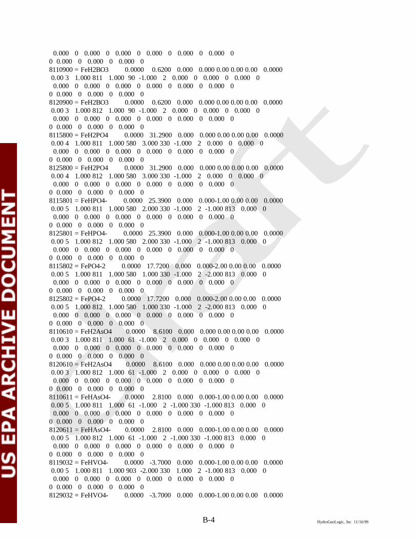
B-4 HydroGeoLogic, Inc 11/16/99
0.000 0 0.000 0 0.000 0 0.000 0 0.000 0 0.000 00 0.000 0 0.000 0 0.000 08110900 =FeH2BO3 0.0000 0.6200 0.000 0.000 0.00 0.00 0.00 0.0000 0.00 3 1.000 811 1.000 90 -1.000 2 0.000 0 0.000 0 0.000 0 0.000 0 0.000 0 0.000 0 0.000 0 0.000 0 0.000 00 0.000 0 0.000 0 0.000 08120900 =FeH2BO3 0.0000 0.6200 0.000 0.000 0.00 0.00 0.00 0.0000 0.00 3 1.000 812 1.000 90 -1.000 2 0.000 0 0.000 0 0.000 0 0.000 0 0.000 0 0.000 0 0.000 0 0.000 0 0.000 00 0.000 0 0.000 0 0.000 08115800 =FeH2PO4 0.0000 31.2900 0.000 0.000 0.00 0.00 0.00 0.0000 0.00 4 1.000 811 1.000 580 3.000 330 -1.000 2 0.000 0 0.000 0 0.000 0 0.000 0 0.000 0 0.000 0 0.000 0 0.000 00 0.000 0 0.000 0 0.000 08125800 =FeH2PO4 0.0000 31.2900 0.000 0.000 0.00 0.00 0.00 0.0000 0.00 4 1.000 812 1.000 580 3.000 330 -1.000 2 0.000 0 0.000 0 0.000 0 0.000 0 0.000 0 0.000 0 0.000 0 0.000 00 0.000 0 0.000 0 0.000 08115801 =FeHPO4- 0.0000 25.3900 0.000 0.000-1.00 0.00 0.00 0.0000 0.00 5 1.000 811 1.000 580 2.000 330 -1.000 2 -1.000 813 0.000 0 0.000 0 0.000 0 0.000 0 0.000 0 0.000 0 0.000 00 0.000 0 0.000 0 0.000 08125801 =FeHPO4- 0.0000 25.3900 0.000 0.000-1.00 0.00 0.00 0.0000 0.00 5 1.000 812 1.000 580 2.000 330 -1.000 2 -1.000 813 0.000 0 0.000 0 0.000 0 0.000 0 0.000 0 0.000 0 0.000 00 0.000 0 0.000 0 0.000 08115802 =FePO4-2 0.0000 17.7200 0.000 0.000-2.00 0.00 0.00 0.0000 0.00 5 1.000 811 1.000 580 1.000 330 -1.000 2 -2.000 813 0.000 0 0.000 0 0.000 0 0.000 0 0.000 0 0.000 0 0.000 00 0.000 0 0.000 0 0.000 08125802 =FePO4-2 0.0000 17.7200 0.000 0.000-2.00 0.00 0.00 0.0000 0.00 5 1.000 812 1.000 580 1.000 330 -1.000 2 -2.000 813 0.000 0 0.000 0 0.000 0 0.000 0 0.000 0 0.000 0 0.000 00 0.000 0 0.000 0 0.000 08110610 =FeH2AsO4 0.0000 8.6100 0.000 0.000 0.00 0.00 0.00 0.0000 0.00 3 1.000 811 1.000 61 -1.000 2 0.000 0 0.000 0 0.000 0 0.000 0 0.000 0 0.000 0 0.000 0 0.000 0 0.000 00 0.000 0 0.000 0 0.000 08120610 =FeH2AsO4 0.0000 8.6100 0.000 0.000 0.00 0.00 0.00 0.0000 0.00 3 1.000 812 1.000 61 -1.000 2 0.000 0 0.000 0 0.000 0 0.000 0 0.000 0 0.000 0 0.000 0 0.000 0 0.000 00 0.000 0 0.000 0 0.000 08110611 =FeHAsO4- 0.0000 2.8100 0.000 0.000-1.00 0.00 0.00 0.0000 0.00 5 1.000 811 1.000 61 -1.000 2 -1.000 330 -1.000 813 0.000 0 0.000 0 0.000 0 0.000 0 0.000 0 0.000 0 0.000 00 0.000 0 0.000 0 0.000 08120611 =FeHAsO4- 0.0000 2.8100 0.000 0.000-1.00 0.00 0.00 0.0000 0.00 5 1.000 812 1.000 61 -1.000 2 -1.000 330 -1.000 813 0.000 0 0.000 0 0.000 0 0.000 0 0.000 0 0.000 0 0.000 00 0.000 0 0.000 0 0.000 08119032 =FeHVO4- 0.0000 -3.7000 0.000 0.000-1.00 0.00 0.00 0.0000 0.00 5 1.000 811 1.000 903 -2.000 330 1.000 2 -1.000 813 0.000 0 0.000 0 0.000 0 0.000 0 0.000 0 0.000 0 0.000 00 0.000 0 0.000 0 0.000 08129032 =FeHVO4- 0.0000 -3.7000 0.000 0.000-1.00 0.00 0.00 0.0000

B-5 HydroGeoLogic, Inc 11/16/99
0.00 5 1.000 812 1.000 903 -2.000 330 1.000 2 -1.000 813 0.000 0 0.000 0 0.000 0 0.000 0 0.000 0 0.000 0 0.000 00 0.000 0 0.000 0 0.000 08117320 =FeSO4- 0.0000 7.7800 0.000 0.000-1.00 0.00 0.00 0.0000 0.00 5 1.000 811 1.000 732 1.000 330 -1.000 2 -1.000 813 0.000 0 0.000 0 0.000 0 0.000 0 0.000 0 0.000 0 0.000 00 0.000 0 0.000 0 0.000 08127320 =FeSO4- 0.0000 7.7800 0.000 0.000-1.00 0.00 0.00 0.0000 0.00 5 1.000 812 1.000 732 1.000 330 -1.000 2 -1.000 813 0.000 0 0.000 0 0.000 0 0.000 0 0.000 0 0.000 0 0.000 00 0.000 0 0.000 0 0.000 08117321 =FeOHSO4-2 0.0000 0.7900 0.000 0.000-2.00 0.00 0.00 0.0000 0.00 3 1.000 811 1.000 732 -2.000 813 0.000 0 0.000 0 0.000 0 0.000 0 0.000 0 0.000 0 0.000 0 0.000 0 0.000 00 0.000 0 0.000 0 0.000 08127321 =FeOHSO4-2 0.0000 0.7900 0.000 0.000-2.00 0.00 0.00 0.0000 0.00 3 1.000 812 1.000 732 -2.000 813 0.000 0 0.000 0 0.000 0 0.000 0 0.000 0 0.000 0 0.000 0 0.000 0 0.000 00 0.000 0 0.000 0 0.000 08117610 =FeSeO3- 0.0000 4.2900 0.000 0.000-1.00 0.00 0.00 0.0000 0.00 4 1.000 811 1.000 761 -1.000 2 -1.000 813 0.000 0 0.000 0 0.000 0 0.000 0 0.000 0 0.000 0 0.000 0 0.000 00 0.000 0 0.000 0 0.000 08127610 =FeSeO3- 0.0000 4.2900 0.000 0.000-1.00 0.00 0.00 0.0000 0.00 4 1.000 812 1.000 761 -1.000 2 -1.000 813 0.000 0 0.000 0 0.000 0 0.000 0 0.000 0 0.000 0 0.000 0 0.000 00 0.000 0 0.000 0 0.000 08117611 =FeOHSeO3-2 0.0000 -3.2300 0.000 0.000-2.00 0.00 0.00 0.0000 0.00 4 1.000 811 1.000 761 -1.000 330 -2.000 813 0.000 0 0.000 0 0.000 0 0.000 0 0.000 0 0.000 0 0.000 0 0.000 00 0.000 0 0.000 0 0.000 08127611 =FeOHSeO3-2 0.0000 -3.2300 0.000 0.000-2.00 0.00 0.00 0.0000 0.00 4 1.000 812 1.000 761 -1.000 330 -2.000 813 0.000 0 0.000 0 0.000 0 0.000 0 0.000 0 0.000 0 0.000 0 0.000 00 0.000 0 0.000 0 0.000 08117620 =FeSeO4- 0.0000 7.7300 0.000 0.000-1.00 0.00 0.00 0.0000 0.00 5 1.000 811 1.000 762 1.000 330 -1.000 2 -1.000 813 0.000 0 0.000 0 0.000 0 0.000 0 0.000 0 0.000 0 0.000 00 0.000 0 0.000 0 0.000 08127620 =FeSeO4- 0.0000 7.7300 0.000 0.000-1.00 0.00 0.00 0.0000 0.00 5 1.000 812 1.000 762 1.000 330 -1.000 2 -1.000 813 0.000 0 0.000 0 0.000 0 0.000 0 0.000 0 0.000 0 0.000 00 0.000 0 0.000 0 0.000 08117621 =FeOHSeO4-2 0.0000 0.8000 0.000 0.000-2.00 0.00 0.00 0.0000 0.00 3 1.000 811 1.000 762 -2.000 813 0.000 0 0.000 0 0.000 0 0.000 0 0.000 0 0.000 0 0.000 0 0.000 0 0.000 00 0.000 0 0.000 0 0.000 08127621 =FeOHSeO4-2 0.0000 0.8000 0.000 0.000-2.00 0.00 0.00 0.0000 0.00 3 1.000 812 1.000 762 -2.000 813 0.000 0 0.000 0 0.000 0 0.000 0 0.000 0 0.000 0 0.000 0 0.000 0 0.000 00 0.000 0 0.000 0 0.000 08112120 =FeCrO4- 0.0000 10.8500 0.000 0.000-1.00 0.00 0.00 0.0000 0.00 5 1.000 811 1.000 212 1.000 330 -1.000 2 -1.000 813 0.000 0 0.000 0 0.000 0 0.000 0 0.000 0 0.000 0 0.000 00 0.000 0 0.000 0 0.000 0

B-6 HydroGeoLogic, Inc 11/16/99
8122120 =FeCrO4- 0.0000 10.8500 0.000 0.000-1.00 0.00 0.00 0.0000 0.00 5 1.000 812 1.000 212 1.000 330 -1.000 2 -1.000 813 0.000 0 0.000 0 0.000 0 0.000 0 0.000 0 0.000 0 0.000 00 0.000 0 0.000 0 0.000 08114800 =FeMoO4- 0.0000 9.5000 0.000 0.000-1.00 0.00 0.00 0.0000 0.00 5 1.000 811 1.000 480 1.000 330 -1.000 2 -1.000 813 0.000 0 0.000 0 0.000 0 0.000 0 0.000 0 0.000 0 0.000 00 0.000 0 0.000 0 0.000 08124800 =FeMoO4- 0.0000 9.5000 0.000 0.000-1.00 0.00 0.00 0.0000 0.00 5 1.000 812 1.000 480 1.000 330 -1.000 2 -1.000 813 0.000 0 0.000 0 0.000 0 0.000 0 0.000 0 0.000 0 0.000 00 0.000 0 0.000 0 0.000 08114801 =FeOHMoO4-2 0.0000 2.4000 0.000 0.000-2.00 0.00 0.00 0.0000 0.00 3 1.000 811 1.000 480 -2.000 813 0.000 0 0.000 0 0.000 0 0.000 0 0.000 0 0.000 0 0.000 0 0.000 0 0.000 00 0.000 0 0.000 0 0.000 08124801 =FeOHMoO4-2 0.0000 2.4000 0.000 0.000-2.00 0.00 0.00 0.0000 0.00 3 1.000 812 1.000 480 -2.000 813 0.000 0 0.000 0 0.000 0 0.000 0 0.000 0 0.000 0 0.000 0 0.000 0 0.000 00 0.000 0 0.000 0 0.000 08117410 =FeSbO(OH)4 0.0000 8.4000 0.000 0.000 0.00 0.00 0.00 0.0000 0.00 4 1.000 811 1.000 741 1.000 330 -2.000 2 0.000 0 0.000 0 0.000 0 0.000 0 0.000 0 0.000 0 0.000 0 0.000 00 0.000 0 0.000 0 0.000 08127410 =FeSbO(OH)4 0.0000 8.4000 0.000 0.000 0.00 0.00 0.00 0.0000 0.00 4 1.000 812 1.000 741 1.000 330 -2.000 2 0.000 0 0.000 0 0.000 0 0.000 0 0.000 0 0.000 0 0.000 0 0.000 00 0.000 0 0.000 0 0.000 08117411 =FeOHSbO(OH4 0.0000 1.3000 0.000 0.000-1.00 0.00 0.00 0.0000 0.00 4 1.000 811 1.000 741 -1.000 2 -1.000 813 0.000 0 0.000 0 0.000 0 0.000 0 0.000 0 0.000 0 0.000 0 0.000 00 0.000 0 0.000 0 0.000 08127411 =FeOHSbO(OH4 0.0000 1.3000 0.000 0.000-1.00 0.00 0.00 0.0000 0.00 4 1.000 812 1.000 741 -1.000 2 -1.000 813 0.000 0 0.000 0 0.000 0 0.000 0 0.000 0 0.000 0 0.000 0 0.000 00 0.000 0 0.000 0 0.000 08111430 =FeCN 0.0000 13.0000 0.000 0.000 0.00 0.00 0.00 0.0000 0.00 4 1.000 811 1.000 143 1.000 330 -1.000 2 0.000 0 0.000 0 0.000 0 0.000 0 0.000 0 0.000 0 0.000 0 0.000 00 0.000 0 0.000 0 0.000 08121430 =FeCN 0.0000 13.0000 0.000 0.000 0.00 0.00 0.00 0.0000 0.00 4 1.000 812 1.000 143 1.000 330 -1.000 2 0.000 0 0.000 0 0.000 0 0.000 0 0.000 0 0.000 0 0.000 0 0.000 00 0.000 0 0.000 0 0.000 08111431 =FeOHCN- 0.0000 5.7000 0.000 0.000-1.00 0.00 0.00 0.0000 0.00 3 1.000 811 1.000 143 -1.000 813 0.000 0 0.000 0 0.000 0 0.000 0 0.000 0 0.000 0 0.000 0 0.000 0 0.000 00 0.000 0 0.000 0 0.000 08121431 =FeOHCN- 0.0000 5.7000 0.000 0.000-1.00 0.00 0.00 0.0000 0.00 3 1.000 812 1.000 143 -1.000 813 0.000 0 0.000 0 0.000 0 0.000 0 0.000 0 0.000 0 0.000 0 0.000 0 0.000 00 0.000 0 0.000 0 0.000 0
APPENDIX C
EXAMPLE INPUT FILE FOR THE MINTEQA2MODEL USED TO ESTIMATE PARTITIONING WITH DOC

C-1 HydroGeoLogic, Inc 11/16/99
Compute Kd-DOC in riverwater MXXM: Md Dissolved OM , No FeO Sorbent, No Particulate OM , Md pH16.00 MG/L 0.000 8.90000E-060 1 1 0 2 3 0 0 1 0 0 1 2Co_doc.prn 200 0.00 8.90 144.00 0.000 0.000 0 0 330 0.000E+00 -4.90 y /H+1 200 1.000E-03 -12.32 y /Co+2 150 1.320E+01 -2.92 y /Ca+2 460 3.600E+00 -3.24 y /Mg+2 410 1.200E+00 -4.13 y /K+1 500 5.300E+00 -3.02 y /Na+1 492 6.010E+00 -3.00 y /NO3- 140 5.200E+01 -2.51 y /CO3-2 180 5.700E+00 -3.37 y /Cl-1 732 6.600E+00 -3.58 y /SO4-2 144 0.000E+00 -6.00 y /DOM1 3 1 330 7.3000 0.0000 /H+1

APPENDIX D
EXAMPLE INPUT FILE FOR THE MINTEQA2MODEL USED TO ESTIMATE PARTITIONING WITH WASTE
SYSTEMS
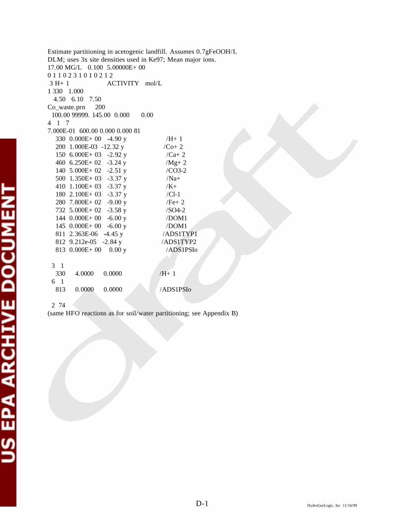
D-1 HydroGeoLogic, Inc 11/16/99
Estimate partitioning in acetogenic landfill. Assumes 0.7gFeOOH/LDLM; uses 3x site densities used in Ke97; Mean major ions. 17.00 MG/L 0.100 5.00000E+000 1 1 0 2 3 1 0 1 0 2 1 2 3 H+1 ACTIVITY mol/L1 330 1.000 4.50 6.10 7.50Co_waste.prn 200 100.00 99999. 145.00 0.000 0.004 1 77.000E-01 600.00 0.000 0.000 81 330 0.000E+00 -4.90 y /H+1 200 1.000E-03 -12.32 y /Co+2 150 6.000E+03 -2.92 y /Ca+2 460 6.250E+02 -3.24 y /Mg+2 140 5.000E+02 -2.51 y /CO3-2 500 1.350E+03 -3.37 y /Na+ 410 1.100E+03 -3.37 y /K+ 180 2.100E+03 -3.37 y /Cl-1 280 7.800E+02 -9.00 y /Fe+2 732 5.000E+02 -3.58 y /SO4-2 144 0.000E+00 -6.00 y /DOM1 145 0.000E+00 -6.00 y /DOM1 811 2.363E-06 -4.45 y /ADS1TYP1 812 9.212e-05 -2.84 y /ADS1TYP2 813 0.000E+00 0.00 y /ADS1PSIo 3 1 330 4.0000 0.0000 /H+1 6 1 813 0.0000 0.0000 /ADS1PSIo 2 74(same HFO reactions as for soil/water partitioning; see Appendix B)

D-2 HydroGeoLogic, Inc 11/16/99
Estimate partitioning in methanogenic landfill. Assumes 0.7gFeOOH/LDLM; uses 3x site densities used in Ke97; Mean major ions. 17.00 MG/L 0.100 5.00000E+000 1 1 0 2 3 1 0 1 0 2 1 2 3 H+1 ACTIVITY mol/L1 330 1.000 7.50 8.00 9.00Co_waste.prn 200 50.00 50000. 145.00 0.000 0.004 1 77.000E-01 600.00 0.000 0.000 81 330 0.000E+00 -4.90 y /H+1 200 1.000E-03 -12.32 y /Co+2 150 9.750E+01 -2.92 y /Ca+2 460 5.000E+02 -3.24 y /Mg+2 140 2.500E+02 -2.51 y /CO3-2 500 1.350E+03 -3.37 y /Na+ 410 1.100E+03 -3.37 y /K+ 180 2.100E+03 -3.37 y /Cl-1 732 8.000E+01 -3.58 y /SO4-2 144 0.000E+00 -6.00 y /DOM1 145 0.000E+00 -6.00 y /DOM1 811 2.363E-06 -4.45 y /ADS1TYP1 812 9.212e-05 -2.84 y /ADS1TYP2 813 0.000E+00 0.00 y /ADS1PSIo 3 1 330 7.0000 0.0000 /H+1 6 1 813 0.0000 0.0000 /ADS1PSIo 2 74(same HFO reactions as for soil/water partitioning; see Appendix B)

D-3 HydroGeoLogic, Inc 11/16/99
Estimate partitioning in MSWI ash monofill. Assumes 0.7gFeOOH/LDLM; uses 3x site densities used in Ke97; Mean major ions. 17.00 MG/L 0.100 5.00000E+000 1 1 0 2 3 1 0 1 0 2 1 2 3 H+1 ACTIVITY mol/L1 330 1.000 8.00 9.00 10.00Co_waste.prn 200 15.00 0. 0.00 0.000 0.004 1 77.000E-01 600.00 0.000 0.000 81 330 0.000E+00 -4.90 y /H+1 200 1.000E-03 -12.32 y /Co+2 150 1.700E+03 -2.92 y /Ca+2 460 1.000E+01 -3.24 y /Mg+2 140 5.000E+01 -2.51 y /CO3-2 500 3.000E+02 -3.37 y /Na+ 410 3.800E+02 -3.37 y /K+ 180 1.200E+03 -3.37 y /Cl-1 732 1.400E+03 -3.58 y /SO4-2 144 0.000E+00 -6.00 y /DOM1 811 2.363E-06 -4.45 y /ADS1TYP1 812 9.212e-05 -2.84 y /ADS1TYP2 813 0.000E+00 0.00 y /ADS1PSIo 3 1 330 4.0000 0.0000 /H+1 6 1 813 0.0000 0.0000 /ADS1PSIo 2 74(same HFO reactions as for soil/water partitioning; see Appendix B)

D-4 HydroGeoLogic, Inc 11/16/99
Estimate partitioning in CKD monofill. Assumes 7.0gFeOOH/LDLM; uses 3x site densities used in Ke97; Mean major ions. 17.00 MG/L 0.100 5.00000E+000 1 1 0 2 3 1 0 1 0 2 1 2 3 H+1 ACTIVITY mol/L1 330 1.000 9.00 10.00 11.00Co_waste.prn 200 15.00 0. 0.00 0.000 0.004 1 77.000E-00 600.00 0.000 0.000 81 330 0.000E+00 -4.90 y /H+1 200 1.000E-03 -12.32 y /Co+2 150 2.850E+03 -2.92 y /Ca+2 460 1.000E+01 -3.24 y /Mg+2 140 5.000E+01 -2.51 y /CO3-2 500 3.000E+02 -3.37 y /Na+ 410 4.000E+02 -3.37 y /K+ 180 3.800E+02 -3.37 y /Cl-1 732 6.300E+02 -3.58 y /SO4-2 144 0.000E+00 -6.00 y /DOM1 811 2.363E-05 -4.45 y /ADS1TYP1 812 9.212e-04 -2.84 y /ADS1TYP2 813 0.000E+00 0.00 y /ADS1PSIo 3 1 330 4.0000 0.0000 /H+1 6 1 813 0.0000 0.0000 /ADS1PSIo 2 74(same HFO reactions as for soil/water partitioning; see Appendix B)

3-10 HydroGeoLogic, Inc 11/16/99