Embed Size (px)
Citation preview

Part II
Motion Planning
Steven M. LaValle
University of Illinois
Copyright Steven M. LaValle 2006
Available for downloading at http://planning.cs.uiuc.edu/
Published by Cambridge University Press
79
Overview of Part II: Motion Planning
Planning in Continuous Spaces
Part II makes the transition from discrete to continuous state spaces. Two al-ternative titles are appropriate for this part: 1) motion planning, or 2) planningin continuous state spaces. Chapters 3–8 are based on research from the field ofmotion planning, which has been building since the 1970s; therefore, the namemotion planning is widely known to refer to the collection of models and algo-rithms that will be covered. On the other hand, it is convenient to also think ofPart II as planning in continuous spaces because this is the primary distinctionwith respect to most other forms of planning.
In addition, motion planning will frequently refer to motions of a robot in a2D or 3D world that contains obstacles. The robot could model an actual robot,or any other collection of moving bodies, such as humans or flexible molecules. Amotion plan involves determining what motions are appropriate for the robot sothat it reaches a goal state without colliding into obstacles. Recall the examplesfrom Section 1.2.
Many issues that arose in Chapter 2 appear once again in motion planning.Two themes that may help to see the connection are as follows.
1. Implicit representations
A familiar theme from Chapter 2 is that planning algorithms must deal with im-plicit representations of the state space. In motion planning, this will becomeeven more important because the state space is uncountably infinite. Further-more, a complicated transformation exists between the world in which the modelsare defined and the space in which the planning occurs. Chapter 3 covers ways tomodel motion planning problems, which includes defining 2D and 3D geometricmodels and transforming them. Chapter 4 introduces the state space that arisesfor these problems. Following motion planning literature [344, 304], we will referto this state space as the configuration space. The dimension of the configura-tion space corresponds to the number of degrees of freedom of the robot. Usingthe configuration space, motion planning will be viewed as a kind of search ina high-dimensional configuration space that contains implicitly represented ob-stacles. One additional complication is that configuration spaces have unusualtopological structure that must be correctly characterized to ensure correct oper-ation of planning algorithms. A motion plan will then be defined as a continuouspath in the configuration space.
2. Continuous → discrete
A central theme throughout motion planning is to transform the continuous modelinto a discrete one. Due to this transformation, many algorithms from Chapter
80
2 are embedded in motion planning algorithms. There are two alternatives toachieving this transformation, which are covered in Chapters 5 and 6, respec-tively. Chapter 6 covers combinatorial motion planning, which means that fromthe input model the algorithms build a discrete representation that exactly repre-sents the original problem. This leads to complete planning approaches, which areguaranteed to find a solution when it exists, or correctly report failure if one doesnot exist. Chapter 5 covers sampling-based motion planning, which refers to algo-rithms that use collision detection methods to sample the configuration space andconduct discrete searches that utilize these samples. In this case, completeness issacrificed, but it is often replaced with a weaker notion, such as resolution com-pleteness or probabilistic completeness. It is important to study both Chapters 5and 6 because each methodology has its strengths and weaknesses. Combinatorialmethods can solve virtually any motion planning problem, and in some restrictedcases, very elegant solutions may be efficiently constructed in practice. However,for the majority of “industrial-grade” motion planning problems, the runningtimes and implementation difficulties of these algorithms make them unappeal-ing. Sampling-based algorithms have fulfilled much of this need in recent yearsby solving challenging problems in several settings, such as automobile assembly,humanoid robot planning, and conformational analysis in drug design. Althoughthe completeness guarantees are weaker, the efficiency and ease of implementationof these methods have bolstered interest in applying motion planning algorithmsto a wide variety of applications.
Two additional chapters appear in Part II. Chapter 7 covers several exten-sions of the basic motion planning problem from the earlier chapters. Theseextensions include avoiding moving obstacles, multiple robot coordination, ma-nipulation planning, and planning with closed kinematic chains. Algorithms thatsolve these problems build on the principles of earlier chapters, but each extensioninvolves new challenges.
Chapter 8 is a transitional chapter that involves many elements of motionplanning but is additionally concerned with gracefully recovering from unexpecteddeviations during execution. Although uncertainty in predicting the future is notexplicitly modeled until Part III, Chapter 8 redefines the notion of a plan to bea function over state space, as opposed to being a path through it. The functiongives the appropriate actions to take during exection, regardless of what con-figuration is entered. This allows the true configuration to drift away from thecommanded configuration. In Part III such uncertainties will be explicitly mod-eled, but this comes at greater modeling and computational costs. It is worthwhileto develop effective ways to avoid this.

Chapter 3
Geometric Representations andTransformations
This chapter provides important background material that will be needed for PartII. Formulating and solving motion planning problems require defining and ma-nipulating complicated geometric models of a system of bodies in space. Section3.1 introduces geometric modeling, which focuses mainly on semi-algebraic mod-eling because it is an important part of Chapter 6. If your interest is mainlyin Chapter 5, then understanding semi-algebraic models is not critical. Sections3.2 and 3.3 describe how to transform a single body and a chain of bodies, re-spectively. This will enable the robot to “move.” These sections are essential forunderstanding all of Part II and many sections beyond. It is expected that manyreaders will already have some or all of this background (especially Section 3.2,but it is included for completeness). Section 3.4 extends the framework for trans-forming chains of bodies to transforming trees of bodies, which allows modelingof complicated systems, such as humanoid robots and flexible organic molecules.Finally, Section 3.5 briefly covers transformations that do not assume each bodyis rigid.
3.1 Geometric Modeling
A wide variety of approaches and techniques for geometric modeling exist, andthe particular choice usually depends on the application and the difficulty of theproblem. In most cases, there are generally two alternatives: 1) a boundary repre-sentation, and 2) a solid representation. Suppose we would like to define a modelof a planet. Using a boundary representation, we might write the equation of asphere that roughly coincides with the planet’s surface. Using a solid represen-tation, we would describe the set of all points that are contained in the sphere.Both alternatives will be considered in this section.
The first step is to define the worldW for which there are two possible choices:1) a 2D world, in which W = R2, and 2) a 3D world, in which W = R3. These
81
82 S. M. LaValle: Planning Algorithms
choices should be sufficient for most problems; however, one might also want toallow more complicated worlds, such as the surface of a sphere or even a higherdimensional space. Such generalities are avoided in this book because their currentapplications are limited. Unless otherwise stated, the world generally contains twokinds of entities:
1. Obstacles: Portions of the world that are “permanently” occupied, forexample, as in the walls of a building.
2. Robots: Bodies that are modeled geometrically and are controllable via amotion plan.
Based on the terminology, one obvious application is to model a robot that movesaround in a building; however, many other possibilities exist. For example, therobot could be a flexible molecule, and the obstacles could be a folded protein.As another example, the robot could be a virtual human in a graphical simulationthat involves obstacles (imagine the family of Doom-like video games).
This section presents a method for systematically constructing representationsof obstacles and robots using a collection of primitives. Both obstacles and robotswill be considered as (closed) subsets of W . Let the obstacle region O denote theset of all points in W that lie in one or more obstacles; hence, O ⊆ W . Thenext step is to define a systematic way of representing O that has great expressivepower while being computationally efficient. Robots will be defined in a similarway; however, this will be deferred until Section 3.2, where transformations ofgeometric bodies are defined.
3.1.1 Polygonal and Polyhedral Models
In this and the next subsection, a solid representation of O will be developed interms of a combination of primitives. Each primitive Hi represents a subset of Wthat is easy to represent and manipulate in a computer. A complicated obstacleregion will be represented by taking finite, Boolean combinations of primitives.Using set theory, this implies thatO can also be defined in terms of a finite numberof unions, intersections, and set differences of primitives.
Convex polygons First consider O for the case in which the obstacle region isa convex, polygonal subset of a 2D world, W = R2. A subset X ⊂ Rn is calledconvex if and only if, for any pair of points in X, all points along the line segmentthat connects them are contained in X. More precisely, this means that for anyx1, x2 ∈ X and λ ∈ [0, 1],
λx1 + (1− λ)x2 ∈ X. (3.1)
Thus, interpolation between x1 and x2 always yields points in X. Intuitively, Xcontains no pockets or indentations. A set that is not convex is called nonconvex(as opposed to concave, which seems better suited for lenses).

3.1. GEOMETRIC MODELING 83
Figure 3.1: A convex polygonal region can be identified by the intersection ofhalf-planes.
A boundary representation of O is anm-sided polygon, which can be describedusing two kinds of features: vertices and edges. Every vertex corresponds to a“corner” of the polygon, and every edge corresponds to a line segment between apair of vertices. The polygon can be specified by a sequence, (x1, y1), (x2, y2), . . .,(xm, ym), of m points in R2, given in counterclockwise order.
A solid representation of O can be expressed as the intersection of m half-planes. Each half-plane corresponds to the set of all points that lie to one sideof a line that is common to a polygon edge. Figure 3.1 shows an example of anoctagon that is represented as the intersection of eight half-planes.
An edge of the polygon is specified by two points, such as (x1, y1) and (x2, y2).Consider the equation of a line that passes through (x1, y1) and (x2, y2). Anequation can be determined of the form ax + by + c = 0, in which a, b, c ∈ R
are constants that are determined from x1, y1, x2, and y2. Let f : R2 → R bethe function given by f(x, y) = ax + by + c. Note that f(x, y) < 0 on one sideof the line, and f(x, y) > 0 on the other. (In fact, f may be interpreted as asigned Euclidean distance from (x, y) to the line.) The sign of f(x, y) indicates ahalf-plane that is bounded by the line, as depicted in Figure 3.2. Without loss ofgenerality, assume that f(x, y) is defined so that f(x, y) < 0 for all points to theleft of the edge from (x1, y1) to (x2, y2) (if it is not, then multiply f(x, y) by −1).
Let fi(x, y) denote the f function derived from the line that corresponds tothe edge from (xi, yi) to (xi+1, yi+1) for 1 ≤ i < m. Let fm(x, y) denote the lineequation that corresponds to the edge from (xm, ym) to (x1, y1). Let a half-plane
84 S. M. LaValle: Planning Algorithms
++
++
++
+
+
−
−
−
−
−−
−−
−−
Figure 3.2: The sign of the f(x, y) partitions R2 into three regions: two half-planesgiven by f(x, y) < 0 and f(x, y) > 0, and the line f(x, y) = 0.
Hi for 1 ≤ i ≤ m be defined as a subset of W :
Hi = (x, y) ∈ W | fi(x, y) ≤ 0. (3.2)
Above, Hi is a primitive that describes the set of all points on one side of theline fi(x, y) = 0 (including the points on the line). A convex, m-sided, polygonalobstacle region O is expressed as
O = H1 ∩H2 ∩ · · · ∩Hm. (3.3)
Nonconvex polygons The assumption that O is convex is too limited for mostapplications. Now suppose that O is a nonconvex, polygonal subset ofW . In thiscase O can be expressed as
O = O1 ∪ O2 ∪ · · · ∪ On, (3.4)
in which each Oi is a convex, polygonal set that is expressed in terms of half-planes using (3.3). Note that Oi and Oj for i 6= j need not be disjoint. Using thisrepresentation, very complicated obstacle regions in W can be defined. Althoughthese regions may contain multiple components and holes, if O is bounded (i.e., Owill fit inside of a big enough rectangular box), its boundary will consist of linearsegments.
In general, more complicated representations of O can be defined in terms ofany finite combination of unions, intersections, and set differences of primitives;however, it is always possible to simplify the representation into the form givenby (3.3) and (3.4). A set difference can be avoided by redefining the primitive.Suppose the model requires removing a set defined by a primitiveHi that contains
1
fi(x, y) < 0. This is equivalent to keeping all points such that fi(x, y) ≥ 0, which isequivalent to −fi(x, y) ≤ 0. This can be used to define a new primitive H ′
i, which
1In this section, we want the resulting set to include all of the points along the boundary.Therefore, < is used to model a set for removal, as opposed to ≤.
3.1. GEOMETRIC MODELING 85
when taken in union with other sets, is equivalent to the removal of Hi. Givena complicated combination of primitives, once set differences are removed, theexpression can be simplified into a finite union of finite intersections by applyingBoolean algebra laws.
Note that the representation of a nonconvex polygon is not unique. Thereare many ways to decompose O into convex components. The decompositionshould be carefully selected to optimize computational performance in whateveralgorithms that model will be used. In most cases, the components may even beallowed to overlap. Ideally, it seems that it would be nice to represent O with theminimum number of primitives, but automating such a decomposition may lead toan NP-hard problem (see Section 6.5.1 for a brief overview of NP-hardness). Oneefficient, practical way to decompose O is to apply the vertical cell decompositionalgorithm, which will be presented in Section 6.2.2
Defining a logical predicate What is the value of the previous representation?As a simple example, we can define a logical predicate that serves as a collisiondetector. Recall from Section 2.4.1 that a predicate is a Boolean-valued function.Let φ be a predicate defined as φ :W → true, false, which returns true fora point in W that lies in O, and false otherwise. For a line given by f(x, y) =0, let e(x, y) denote a logical predicate that returns true if f(x, y) ≤ 0, andfalse otherwise.
A predicate that corresponds to a convex polygonal region is represented by alogical conjunction,
α(x, y) = e1(x, y) ∧ e2(x, y) ∧ · · · ∧ em(x, y). (3.5)
The predicate α(x, y) returns true if the point (x, y) lies in the convex polyg-onal region, and false otherwise. An obstacle region that consists of n convexpolygons is represented by a logical disjunction of conjuncts,
φ(x, y) = α1(x, y) ∨ α2(x, y) ∨ · · · ∨ αn(x, y). (3.6)
Although more efficient methods exist, φ can check whether a point (x, y) liesin O in time O(n), in which n is the number of primitives that appear in therepresentation of O (each primitive is evaluated in constant time).
Note the convenient connection between a logical predicate representation anda set-theoretic representation. Using the logical predicate, the unions and inter-sections of the set-theoretic representation are replaced by logical ORs and ANDs.It is well known from Boolean algebra that any complicated logical sentence canbe reduced to a logical disjunction of conjunctions (this is often called “sum ofproducts” in computer engineering). This is equivalent to our previous statementthat O can always be represented as a union of intersections of primitives.
Polyhedral models For a 3D world, W = R3, and the previous concepts canbe nicely generalized from the 2D case by replacing polygons with polyhedra and
86 S. M. LaValle: Planning Algorithms
replacing half-plane primitives with half-space primitives. A boundary represen-tation can be defined in terms of three features: vertices, edges, and faces. Everyface is a “flat” polygon embedded in R3. Every edge forms a boundary betweentwo faces. Every vertex forms a boundary between three or more edges.
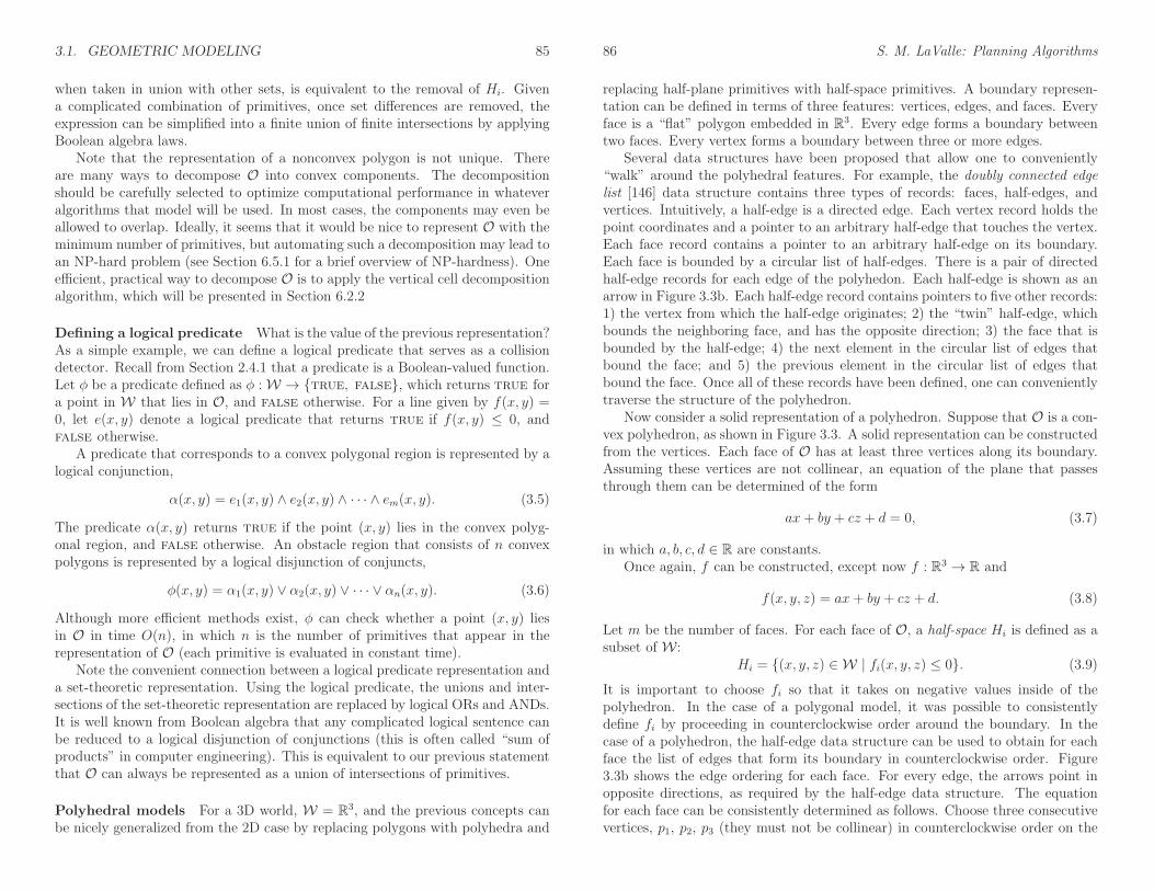
Several data structures have been proposed that allow one to conveniently“walk” around the polyhedral features. For example, the doubly connected edgelist [146] data structure contains three types of records: faces, half-edges, andvertices. Intuitively, a half-edge is a directed edge. Each vertex record holds thepoint coordinates and a pointer to an arbitrary half-edge that touches the vertex.Each face record contains a pointer to an arbitrary half-edge on its boundary.Each face is bounded by a circular list of half-edges. There is a pair of directedhalf-edge records for each edge of the polyhedon. Each half-edge is shown as anarrow in Figure 3.3b. Each half-edge record contains pointers to five other records:1) the vertex from which the half-edge originates; 2) the “twin” half-edge, whichbounds the neighboring face, and has the opposite direction; 3) the face that isbounded by the half-edge; 4) the next element in the circular list of edges thatbound the face; and 5) the previous element in the circular list of edges thatbound the face. Once all of these records have been defined, one can convenientlytraverse the structure of the polyhedron.
Now consider a solid representation of a polyhedron. Suppose that O is a con-vex polyhedron, as shown in Figure 3.3. A solid representation can be constructedfrom the vertices. Each face of O has at least three vertices along its boundary.Assuming these vertices are not collinear, an equation of the plane that passesthrough them can be determined of the form
ax+ by + cz + d = 0, (3.7)
in which a, b, c, d ∈ R are constants.Once again, f can be constructed, except now f : R3 → R and
f(x, y, z) = ax+ by + cz + d. (3.8)
Let m be the number of faces. For each face of O, a half-space Hi is defined as asubset of W :
Hi = (x, y, z) ∈ W | fi(x, y, z) ≤ 0. (3.9)
It is important to choose fi so that it takes on negative values inside of thepolyhedron. In the case of a polygonal model, it was possible to consistentlydefine fi by proceeding in counterclockwise order around the boundary. In thecase of a polyhedron, the half-edge data structure can be used to obtain for eachface the list of edges that form its boundary in counterclockwise order. Figure3.3b shows the edge ordering for each face. For every edge, the arrows point inopposite directions, as required by the half-edge data structure. The equationfor each face can be consistently determined as follows. Choose three consecutivevertices, p1, p2, p3 (they must not be collinear) in counterclockwise order on the
3.1. GEOMETRIC MODELING 87
(a) (b)
Figure 3.3: (a) A polyhedron can be described in terms of faces, edges, andvertices. (b) The edges of each face can be stored in a circular list that is traversedin counterclockwise order with respect to the outward normal vector of the face.
boundary of the face. Let v12 denote the vector from p1 to p2, and let v23 denotethe vector from p2 to p3. The cross product v = v12 × v23 always yields a vectorthat points out of the polyhedron and is normal to the face. Recall that the vector[a b c] is parallel to the normal to the plane. If its components are chosen asa = v[1], b = v[2], and c = v[3], then f(x, y, z) ≤ 0 for all points in the half-spacethat contains the polyhedron.
As in the case of a polygonal model, a convex polyhedron can be defined asthe intersection of a finite number of half-spaces, one for each face. A nonconvexpolyhedron can be defined as the union of a finite number of convex polyhedra.The predicate φ(x, y, z) can be defined in a similar manner, in this case yieldingtrue if (x, y, z) ∈ O, and false otherwise.
3.1.2 Semi-Algebraic Models
In both the polygonal and polyhedral models, f was a linear function. In thecase of a semi-algebraic model for a 2D world, f can be any polynomial withreal-valued coefficients and variables x and y. For a 3D world, f is a polynomialwith variables x, y, and z. The class of semi-algebraic models includes bothpolygonal and polyhedral models, which use first-degree polynomials. A point setdetermined by a single polynomial primitive is called an algebraic set; a point setthat can be obtained by a finite number of unions and intersections of algebraicsets is called a semi-algebraic set.
Consider the case of a 2D world. A solid representation can be defined using
88 S. M. LaValle: Planning Algorithms
++
++
++
++−
−
−−
−−
−−
++
+++
++
++++
++
(a) (b)
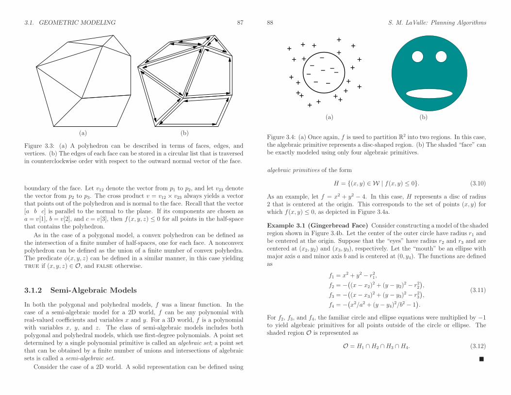
Figure 3.4: (a) Once again, f is used to partition R2 into two regions. In this case,the algebraic primitive represents a disc-shaped region. (b) The shaded “face” canbe exactly modeled using only four algebraic primitives.
algebraic primitives of the form
H = (x, y) ∈ W | f(x, y) ≤ 0. (3.10)
As an example, let f = x2 + y2 − 4. In this case, H represents a disc of radius2 that is centered at the origin. This corresponds to the set of points (x, y) forwhich f(x, y) ≤ 0, as depicted in Figure 3.4a.
Example 3.1 (Gingerbread Face) Consider constructing a model of the shadedregion shown in Figure 3.4b. Let the center of the outer circle have radius r1 andbe centered at the origin. Suppose that the “eyes” have radius r2 and r3 and arecentered at (x2, y2) and (x3, y3), respectively. Let the “mouth” be an ellipse withmajor axis a and minor axis b and is centered at (0, y4). The functions are definedas
f1 = x2 + y2 − r21,f2 = −
(
(x− x2)2 + (y − y2)2 − r22)
,
f3 = −(
(x− x3)2 + (y − y3)2 − r23)
,
f4 = −(
x2/a2 + (y − y4)2/b2 − 1)
.
(3.11)
For f2, f3, and f4, the familiar circle and ellipse equations were multiplied by −1to yield algebraic primitives for all points outside of the circle or ellipse. Theshaded region O is represented as
O = H1 ∩H2 ∩H3 ∩H4. (3.12)

3.1. GEOMETRIC MODELING 89
In the case of semi-algebraic models, the intersection of primitives does notnecessarily result in a convex subset of W . In general, however, it might benecessary to form O by taking unions and intersections of algebraic primitives.
A logical predicate, φ(x, y), can once again be formed, and collision checkingis still performed in time that is linear in the number of primitives. Note thatit is still very efficient to evaluate every primitive; f is just a polynomial that isevaluated on the point (x, y, z).
The semi-algebraic formulation generalizes easily to the case of a 3D world.This results in algebraic primitives of the form
H = (x, y, z) ∈ W | f(x, y, z) ≤ 0, (3.13)
which can be used to define a solid representation of a 3D obstacle O and a logicalpredicate φ.
Equations (3.10) and (3.13) are sufficient to express any model of interest. Onemay define many other primitives based on different relations, such as f(x, y, z) ≥0, f(x, y, z) = 0, f(x, y, z) < 0, f(x, y, z) = 0, and f(x, y, z) 6= 0; however, mostof them do not enhance the set of models that can be expressed. They might,however, be more convenient in certain contexts. To see that some primitives donot allow new models to be expressed, consider the primitive
H = (x, y, z) ∈ W | f(x, y, z) ≥ 0. (3.14)
The right part may be alternatively represented as −f(x, y, z) ≤ 0, and −f maybe considered as a new polynomial function of x, y, and z. For an example thatinvolves the = relation, consider the primitive
H = (x, y, z) ∈ W | f(x, y, z) = 0. (3.15)
It can instead be constructed as H = H1 ∩H2, in which
H1 = (x, y, z) ∈ W | f(x, y, z) ≤ 0 (3.16)
and
H2 = (x, y, z) ∈ W | − f(x, y, z) ≤ 0. (3.17)
The relation < does add some expressive power if it is used to construct primi-tives.2 It is needed to construct models that do not include the outer boundary(for example, the set of all points inside of a sphere, which does not include pointson the sphere). These are generally called open sets and are defined Chapter 4.
2An alternative that yields the same expressive power is to still use ≤, but allow set comple-ments, in addition to unions and intersections.
90 S. M. LaValle: Planning Algorithms
Figure 3.5: A polygon with holes can be expressed by using different orientations:counterclockwise for the outer boundary and clockwise for the hole boundaries.Note that the shaded part is always to the left when following the arrows.
3.1.3 Other Models
The choice of a model often depends on the types of operations that will be per-formed by the planning algorithm. For combinatorial motion planning methods,to be covered in Chapter 6, the particular representation is critical. On the otherhand, for sampling-based planning methods, to be covered in Chapter 5, the par-ticular representation is important only to the collision detection algorithm, whichis treated as a “black box” as far as planning is concerned. Therefore, the modelsgiven in the remainder of this section are more likely to appear in sampling-basedapproaches and may be invisible to the designer of a planning algorithm (althoughit is never wise to forget completely about the representation).
Nonconvex polygons and polyhedra The method in Section 3.1.1 requirednonconvex polygons to be represented as a union of convex polygons. Instead, aboundary representation of a nonconvex polygon may be directly encoded by list-ing vertices in a specific order; assume that counterclockwise order is used. Eachpolygon of m vertices may be encoded by a list of the form (x1, y1), (x2, y2), . . .,(xm, ym). It is assumed that there is an edge between each (xi, yi) and (xi+1, yi+1)for each i from 1 to m − 1, and also an edge between (xm, ym) and (x1, y1). Or-dinarily, the vertices should be chosen in a way that makes the polygon simple,meaning that no edges intersect. In this case, there is a well-defined interior ofthe polygon, which is to the left of every edge, if the vertices are listed in coun-terclockwise order.
What if a polygon has a hole in it? In this case, the boundary of the holecan be expressed as a polygon, but with its vertices appearing in the clockwisedirection. To the left of each edge is the interior of the outer polygon, and to theright is the hole, as shown in Figure 3.5
Although the data structures are a little more complicated for three dimen-sions, boundary representations of nonconvex polyhedra may be expressed in a
3.1. GEOMETRIC MODELING 91
Figure 3.6: Triangle strips and triangle fans can reduce the number of redundantpoints.
similar manner. In this case, instead of an edge list, one must specify faces, edges,and vertices, with pointers that indicate their incidence relations. Consistent ori-entations must also be chosen, and holes may be modeled once again by selectingopposite orientations.
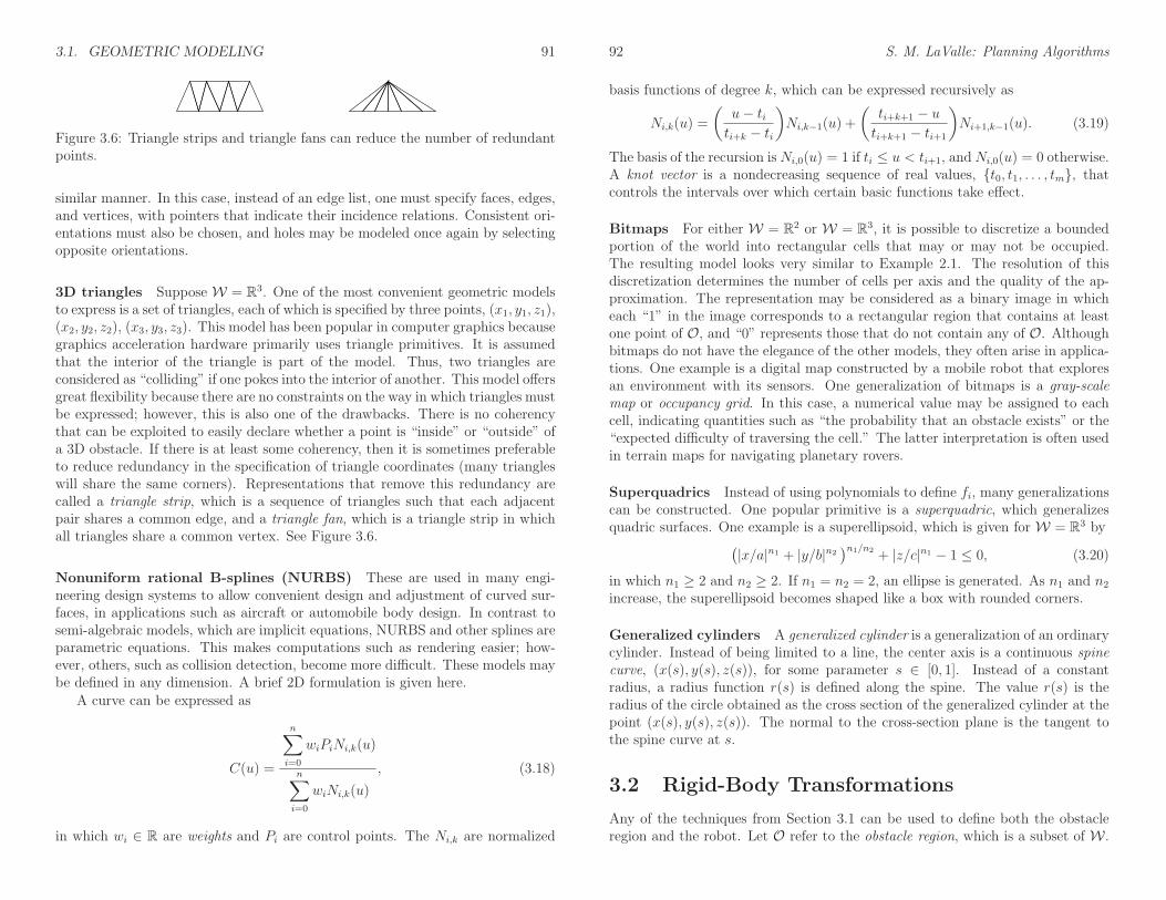
3D triangles Suppose W = R3. One of the most convenient geometric modelsto express is a set of triangles, each of which is specified by three points, (x1, y1, z1),(x2, y2, z2), (x3, y3, z3). This model has been popular in computer graphics becausegraphics acceleration hardware primarily uses triangle primitives. It is assumedthat the interior of the triangle is part of the model. Thus, two triangles areconsidered as “colliding” if one pokes into the interior of another. This model offersgreat flexibility because there are no constraints on the way in which triangles mustbe expressed; however, this is also one of the drawbacks. There is no coherencythat can be exploited to easily declare whether a point is “inside” or “outside” ofa 3D obstacle. If there is at least some coherency, then it is sometimes preferableto reduce redundancy in the specification of triangle coordinates (many triangleswill share the same corners). Representations that remove this redundancy arecalled a triangle strip, which is a sequence of triangles such that each adjacentpair shares a common edge, and a triangle fan, which is a triangle strip in whichall triangles share a common vertex. See Figure 3.6.
Nonuniform rational B-splines (NURBS) These are used in many engi-neering design systems to allow convenient design and adjustment of curved sur-faces, in applications such as aircraft or automobile body design. In contrast tosemi-algebraic models, which are implicit equations, NURBS and other splines areparametric equations. This makes computations such as rendering easier; how-ever, others, such as collision detection, become more difficult. These models maybe defined in any dimension. A brief 2D formulation is given here.
A curve can be expressed as
C(u) =
n∑
i=0
wiPiNi,k(u)
n∑
i=0
wiNi,k(u)
, (3.18)
in which wi ∈ R are weights and Pi are control points. The Ni,k are normalized
92 S. M. LaValle: Planning Algorithms
basis functions of degree k, which can be expressed recursively as
Ni,k(u) =
(
u− titi+k − ti
)
Ni,k−1(u) +
(
ti+k+1 − uti+k+1 − ti+1
)
Ni+1,k−1(u). (3.19)
The basis of the recursion isNi,0(u) = 1 if ti ≤ u < ti+1, andNi,0(u) = 0 otherwise.A knot vector is a nondecreasing sequence of real values, t0, t1, . . . , tm, thatcontrols the intervals over which certain basic functions take effect.
Bitmaps For either W = R2 or W = R3, it is possible to discretize a boundedportion of the world into rectangular cells that may or may not be occupied.The resulting model looks very similar to Example 2.1. The resolution of thisdiscretization determines the number of cells per axis and the quality of the ap-proximation. The representation may be considered as a binary image in whicheach “1” in the image corresponds to a rectangular region that contains at leastone point of O, and “0” represents those that do not contain any of O. Althoughbitmaps do not have the elegance of the other models, they often arise in applica-tions. One example is a digital map constructed by a mobile robot that exploresan environment with its sensors. One generalization of bitmaps is a gray-scalemap or occupancy grid. In this case, a numerical value may be assigned to eachcell, indicating quantities such as “the probability that an obstacle exists” or the“expected difficulty of traversing the cell.” The latter interpretation is often usedin terrain maps for navigating planetary rovers.
Superquadrics Instead of using polynomials to define fi, many generalizationscan be constructed. One popular primitive is a superquadric, which generalizesquadric surfaces. One example is a superellipsoid, which is given for W = R3 by
(
|x/a|n1 + |y/b|n2)n1/n2 + |z/c|n1 − 1 ≤ 0, (3.20)
in which n1 ≥ 2 and n2 ≥ 2. If n1 = n2 = 2, an ellipse is generated. As n1 and n2
increase, the superellipsoid becomes shaped like a box with rounded corners.
Generalized cylinders A generalized cylinder is a generalization of an ordinarycylinder. Instead of being limited to a line, the center axis is a continuous spinecurve, (x(s), y(s), z(s)), for some parameter s ∈ [0, 1]. Instead of a constantradius, a radius function r(s) is defined along the spine. The value r(s) is theradius of the circle obtained as the cross section of the generalized cylinder at thepoint (x(s), y(s), z(s)). The normal to the cross-section plane is the tangent tothe spine curve at s.
3.2 Rigid-Body Transformations
Any of the techniques from Section 3.1 can be used to define both the obstacleregion and the robot. Let O refer to the obstacle region, which is a subset of W .
3.2. RIGID-BODY TRANSFORMATIONS 93
Let A refer to the robot, which is a subset of R2 or R3, matching the dimensionof W . Although O remains fixed in the world, W , motion planning problems willrequire “moving” the robot, A.
3.2.1 General Concepts
Before giving specific transformations, it will be helpful to define them in general toavoid confusion in later parts when intuitive notions might fall apart. Suppose thata rigid robot, A, is defined as a subset of R2 or R3. A rigid-body transformation isa function, h : A →W , that maps every point of A intoW with two requirements:1) The distance between any pair of points of A must be preserved, and 2) theorientation of A must be preserved (no “mirror images”).
Using standard function notation, h(a) for some a ∈ A refers to the point inW that is “occupied” by a. Let
h(A) = h(a) ∈ W | a ∈ A, (3.21)
which is the image of h and indicates all points inW occupied by the transformedrobot.
Transforming the robot model Consider transforming a robot model. If Ais expressed by naming specific points in R2, as in a boundary representation of apolygon, then each point is simply transformed from a to h(a) ∈ W . In this case,it is straightforward to transform the entire model using h. However, there is aslight complication if the robot model is expressed using primitives, such as
Hi = a ∈ R2 | fi(a) ≤ 0. (3.22)
This differs slightly from (3.2) because the robot is defined in R2 (which is notnecessarily W), and also a is used to denote a point (x, y) ∈ A. Under a trans-formation h, the primitive is transformed as
h(Hi) = h(a) ∈ W | fi(a) ≤ 0. (3.23)
To transform the primitive completely, however, it is better to directly namepoints in w ∈ W , as opposed to h(a) ∈ W . Using the fact that a = h−1(w), thisbecomes
h(Hi) = w ∈ W | fi(h−1(w)) ≤ 0, (3.24)
in which the inverse of h appears in the right side because the original pointa ∈ A needs to be recovered to evaluate fi. Therefore, it is important to becareful because either h or h−1 may be required to transform the model. This willbe observed in more specific contexts in some coming examples.
94 S. M. LaValle: Planning Algorithms
A parameterized family of transformations It will become important tostudy families of transformations, in which some parameters are used to selectthe particular transformation. Therefore, it makes sense to generalize h to accepttwo variables: a parameter vector, q ∈ Rn, along with a ∈ A. The resultingtransformed point a is denoted by h(q, a), and the entire robot is transformed toh(q,A) ⊂ W .
The coming material will use the following shorthand notation, which requiresthe specific h to be inferred from the context. Let h(q, a) be shortened to a(q), andlet h(q,A) be shortened to A(q). This notation makes it appear that by adjustingthe parameter q, the robot A travels around in W as different transformationsare selected from the predetermined family. This is slightly abusive notation, butit is convenient. The expression A(q) can be considered as a set-valued functionthat yields the set of points in W that are occupied by A when it is transformedby q. Most of the time the notation does not cause trouble, but when it does, itis helpful to remember the definitions from this section, especially when trying todetermine whether h or h−1 is needed.
Defining frames It was assumed so far that A is defined in R2 or R3, but beforeit is transformed, it is not considered to be a subset of W . The transformation hplaces the robot in W . In the coming material, it will be convenient to indicatethis distinction using coordinate frames. The origin and coordinate basis vectorsofW will be referred to as the world frame.3 Thus, any point w ∈ W is expressedin terms of the world frame.
The coordinates used to define A are initially expressed in the body frame,which represents the origin and coordinate basis vectors of R2 or R3. In the caseof A ⊂ R2, it can be imagined that the body frame is painted on the robot.Transforming the robot is equivalent to converting its model from the body frameto the world frame. This has the effect of placing4 A into W at some positionand orientation. When multiple bodies are covered in Section 3.3, each body willhave its own body frame, and transformations require expressing all bodies withrespect to the world frame.
3.2.2 2D Transformations
Translation A rigid robotA ⊂ R2 is translated by using two parameters, xt, yt ∈R. Using definitions from Section 3.2.1, q = (xt, yt), and h is defined as
h(x, y) = (x+ xt, y + yt). (3.25)
3The world frame serves the same purpose as an inertial frame in Newtonian mechanics.Intuitively, it is a frame that remains fixed and from which all measurements are taken. SeeSection 13.3.1.
4Technically, this placement is a function called an orientation-preserving isometric embed-
ding.

3.2. RIGID-BODY TRANSFORMATIONS 95
A boundary representation of A can be translated by transforming each vertex inthe sequence of polygon vertices using (3.25). Each point, (xi, yi), in the sequenceis replaced by (xi + xt, yi + yt).
Now consider a solid representation of A, defined in terms of primitives. Eachprimitive of the form
Hi = (x, y) ∈ R2 | f(x, y) ≤ 0 (3.26)
is transformed to
h(Hi) = (x, y) ∈ W | f(x− xt, y − yt) ≤ 0. (3.27)
Example 3.2 (Translating a Disc) For example, suppose the robot is a discof unit radius, centered at the origin. It is modeled by a single primitive,
Hi = (x, y) ∈ R2 | x2 + y2 − 1 ≤ 0. (3.28)
Suppose A = Hi is translated xt units in the x direction and yt units in the ydirection. The transformed primitive is
h(Hi) = (x, y) ∈ W | (x− xt)2 + (y − yt)2 − 1 ≤ 0, (3.29)
which is the familiar equation for a disc centered at (xt, yt). In this example, theinverse, h−1 is used, as described in Section 3.2.1.
The translated robot is denoted as A(xt, yt). Translation by (0, 0) is the iden-tity transformation, which results in A(0, 0) = A, if it is assumed that A ⊂ W(recall that A does not necessarily have to be initially embedded in W). It willbe convenient to use the term degrees of freedom to refer to the maximum numberof independent parameters that are needed to completely characterize the trans-formation applied to the robot. If the set of allowable values for xt and yt formsa two-dimensional subset of R2, then the degrees of freedom is two.
Suppose that A is defined directly in W with translation. As shown in Figure3.7, there are two interpretations of a rigid-body transformation applied to A: 1)The world frame remains fixed and the robot is transformed; 2) the robot remainsfixed and the world frame is translated. The first one characterizes the effect ofthe transformation from a fixed world frame, and the second one indicates howthe transformation appears from the robot’s perspective. Unless stated otherwise,the first interpretation will be used when we refer to motion planning problemsbecause it often models a robot moving in a physical world. Numerous bookscover coordinate transformations under the second interpretation. This has beenknown to cause confusion because the transformations may sometimes appear“backward” from what is desired in motion planning.
96 S. M. LaValle: Planning Algorithms
Movingthe Robot
Moving theCoordinateFrame
(a) Translation of the robot (b) Translation of the frame
Figure 3.7: Every transformation has two interpretations.
Rotation The robot, A, can be rotated counterclockwise by some angle θ ∈[0, 2π) by mapping every (x, y) ∈ A as
(x, y) 7→ (x cos θ − y sin θ, x sin θ + y cos θ). (3.30)
Using a 2× 2 rotation matrix,
R(θ) =
(
cos θ − sin θsin θ cos θ
)
, (3.31)
the transformation can be written as
(
x cos θ − y sin θx sin θ + y cos θ
)
= R(θ)
(
xy
)
. (3.32)
Using the notation of Section 3.2.1, R(θ) becomes h(q), for which q = θ. Forlinear transformations, such as the one defined by (3.32), recall that the columnvectors represent the basis vectors of the new coordinate frame. The columnvectors of R(θ) are unit vectors, and their inner product (or dot product) is zero,indicating that they are orthogonal. Suppose that the x and y coordinate axes,which represent the body frame, are “painted” on A. The columns of R(θ) can bederived by considering the resulting directions of the x- and y-axes, respectively,after performing a counterclockwise rotation by the angle θ. This interpretationgeneralizes nicely for higher dimensional rotation matrices.
Note that the rotation is performed about the origin. Thus, when defining themodel of A, the origin should be placed at the intended axis of rotation. Usingthe semi-algebraic model, the entire robot model can be rotated by transformingeach primitive, yielding A(θ). The inverse rotation, R(−θ), must be applied toeach primitive.

3.2. RIGID-BODY TRANSFORMATIONS 97
Combining translation and rotation Suppose a rotation by θ is performed,followed by a translation by xt, yt. This can be used to place the robot in anydesired position and orientation. Note that translations and rotations do notcommute! If the operations are applied successively, each (x, y) ∈ A is transformedto
(
x cos θ − y sin θ + xtx sin θ + y cos θ + yt
)
. (3.33)
The following matrix multiplication yields the same result for the first two vectorcomponents:
cos θ − sin θ xtsin θ cos θ yt0 0 1
xy1
=
x cos θ − y sin θ + xtx sin θ + y cos θ + yt
1
. (3.34)
This implies that the 3× 3 matrix,
T =
cos θ − sin θ xtsin θ cos θ yt0 0 1
, (3.35)
represents a rotation followed by a translation. The matrix T will be referred toas a homogeneous transformation matrix. It is important to remember that Trepresents a rotation followed by a translation (not the other way around). Eachprimitive can be transformed using the inverse of T , resulting in a transformedsolid model of the robot. The transformed robot is denoted by A(xt, yt, θ), andin this case there are three degrees of freedom. The homogeneous transformationmatrix is a convenient representation of the combined transformations; therefore,it is frequently used in robotics, mechanics, computer graphics, and elsewhere. Itis called homogeneous because over R3 it is just a linear transformation withoutany translation. The trick of increasing the dimension by one to absorb thetranslational part is common in projective geometry [404].
3.2.3 3D Transformations
Rigid-body transformations for the 3D case are conceptually similar to the 2Dcase; however, the 3D case appears more difficult because rotations are signifi-cantly more complicated.
3D translation The robot, A, is translated by some xt, yt, zt ∈ R using
(x, y, z) 7→ (x+ xt, y + yt, z + zt). (3.36)
A primitive of the form
Hi = (x, y, z) ∈ W | fi(x, y, z) ≤ 0 (3.37)
98 S. M. LaValle: Planning Algorithms
Yaw
z
y
x
PitchRoll
γ
β
α
Figure 3.8: Any three-dimensional rotation can be described as a sequence of yaw,pitch, and roll rotations.
is transformed to
(x, y, z) ∈ W | fi(x− xt, y − yt, z − zt) ≤ 0. (3.38)
The translated robot is denoted as A(xt, yt, zt).
Yaw, pitch, and roll rotations A 3D body can be rotated about three or-thogonal axes, as shown in Figure 3.8. Borrowing aviation terminology, theserotations will be referred to as yaw, pitch, and roll:
1. A yaw is a counterclockwise rotation of α about the z-axis. The rotationmatrix is given by
Rz(α) =
cosα − sinα 0sinα cosα 00 0 1
. (3.39)
Note that the upper left entries of Rz(α) form a 2D rotation applied to thex and y coordinates, whereas the z coordinate remains constant.
2. A pitch is a counterclockwise rotation of β about the y-axis. The rotationmatrix is given by
Ry(β) =
cos β 0 sin β0 1 0
− sin β 0 cos β
. (3.40)
3. A roll is a counterclockwise rotation of γ about the x-axis. The rotationmatrix is given by
Rx(γ) =
1 0 00 cos γ − sin γ0 sin γ cos γ
. (3.41)

3.2. RIGID-BODY TRANSFORMATIONS 99
Each rotation matrix is a simple extension of the 2D rotation matrix, (3.31). Forexample, the yaw matrix, Rz(α), essentially performs a 2D rotation with respectto the x and y coordinates while leaving the z coordinate unchanged. Thus, thethird row and third column of Rz(α) look like part of the identity matrix, whilethe upper right portion of Rz(α) looks like the 2D rotation matrix.
The yaw, pitch, and roll rotations can be used to place a 3D body in anyorientation. A single rotation matrix can be formed by multiplying the yaw,pitch, and roll rotation matrices to obtain
R(α,β, γ) = Rz(α)Ry(β)Rx(γ) =
cosα cos β cosα sin β sin γ − sinα cos γ cosα sin β cos γ + sinα sin γsinα cos β sinα sin β sin γ + cosα cos γ sinα sin β cos γ − cosα sin γ− sin β cos β sin γ cos β cos γ
.
(3.42)
It is important to note that R(α, β, γ) performs the roll first, then the pitch, andfinally the yaw. If the order of these operations is changed, a different rotationmatrix would result. Be careful when interpreting the rotations. Consider thefinal rotation, a yaw by α. Imagine sitting inside of a robot A that looks likean aircraft. If β = γ = 0, then the yaw turns the plane in a way that feelslike turning a car to the left. However, for arbitrary values of β and γ, the finalrotation axis will not be vertically aligned with the aircraft because the aircraft isleft in an unusual orientation before α is applied. The yaw rotation occurs aboutthe z-axis of the world frame, not the body frame of A. Each time a new rotationmatrix is introduced from the left, it has no concern for original body frame ofA. It simply rotates every point in R3 in terms of the world frame. Note that 3Drotations depend on three parameters, α, β, and γ, whereas 2D rotations dependonly on a single parameter, θ. The primitives of the model can be transformedusing R(α, β, γ), resulting in A(α, β, γ).
Determining yaw, pitch, and roll from a rotation matrix It is oftenconvenient to determine the α, β, and γ parameters directly from a given rotationmatrix. Suppose an arbitrary rotation matrix
r11 r12 r13r21 r22 r23r31 r32 r33
(3.43)
is given. By setting each entry equal to its corresponding entry in (3.42), equationsare obtained that must be solved for α, β, and γ. Note that r21/r11 = tanα andr32/r33 = tan γ. Also, r31 = − sin β and
√
r232 + r233 = cos β. Solving for eachangle yields
α = tan−1(r21/r11), (3.44)
β = tan−1(
− r31/
√
r232 + r233
)
, (3.45)
100 S. M. LaValle: Planning Algorithms
andγ = tan−1(r32/r33). (3.46)
There is a choice of four quadrants for the inverse tangent functions. How canthe correct quadrant be determined? Each quadrant should be chosen by usingthe signs of the numerator and denominator of the argument. The numeratorsign selects whether the direction will be above or below the x-axis, and thedenominator selects whether the direction will be to the left or right of the y-axis.This is the same as the atan2 function in the C programming language, whichnicely expands the range of the arctangent to [0, 2π). This can be applied toexpress (3.44), (3.45), and (3.46) as
α = atan2(r21, r11), (3.47)
β = atan2(
− r31,√
r232 + r233
)
, (3.48)
andγ = atan2(r32, r33). (3.49)
Note that this method assumes r11 6= 0 and r33 6= 0.
The homogeneous transformation matrix for 3D bodies As in the 2Dcase, a homogeneous transformation matrix can be defined. For the 3D case, a4× 4 matrix is obtained that performs the rotation given by R(α, β, γ), followedby a translation given by xt, yt, zt. The result is
T =
cosα cosβ cosα sinβ sin γ − sinα cos γ cosα sinβ cos γ + sinα sin γ xtsinα cosβ sinα sinβ sin γ + cosα cos γ sinα sinβ cos γ − cosα sin γ yt− sinβ cosβ sin γ cosβ cos γ zt
0 0 0 1
.
(3.50)Once again, the order of operations is critical. The matrix T in (3.50) representsthe following sequence of transformations:
1. Roll by γ 3. Yaw by α2. Pitch by β 4. Translate by (xt, yt, zt).
The robot primitives can be transformed to yield A(xt, yt, zt, α, β, γ). A 3D rigidbody that is capable of translation and rotation therefore has six degrees of free-dom.
3.3 Transforming Kinematic Chains of Bodies
The transformations become more complicated for a chain of attached rigid bodies.For convenience, each rigid body is referred to as a link. Let A1, A2, . . . , Am
denote a set of m links. For each i such that 1 ≤ i < m, link Ai is “attached” to
3.3. TRANSFORMING KINEMATIC CHAINS OF BODIES 101
link Ai+1 in a way that allows Ai+1 some constrained motion with respect to Ai.The motion constraint must be explicitly given, and will be discussed shortly. Asan example, imagine a trailer that is attached to the back of a car by a hitch thatallows the trailer to rotate with respect to the car. In general, a set of attachedbodies will be referred to as a linkage. This section considers bodies that areattached in a single chain. This leads to a particular linkage called a kinematicchain.
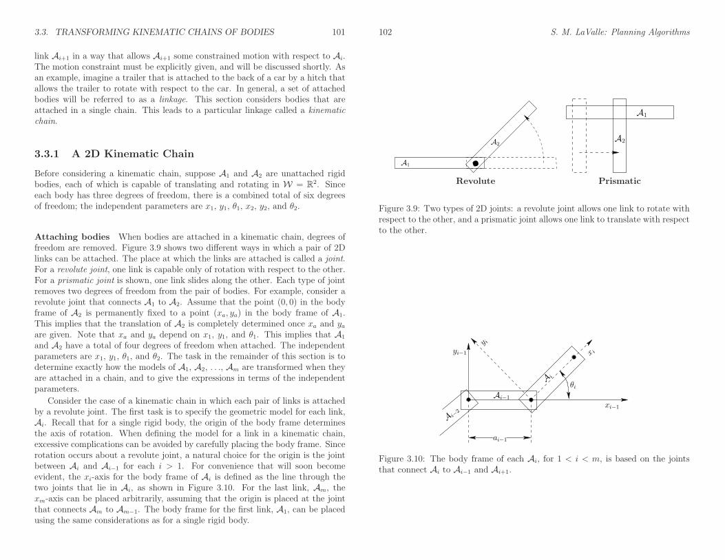
3.3.1 A 2D Kinematic Chain
Before considering a kinematic chain, suppose A1 and A2 are unattached rigidbodies, each of which is capable of translating and rotating in W = R2. Sinceeach body has three degrees of freedom, there is a combined total of six degreesof freedom; the independent parameters are x1, y1, θ1, x2, y2, and θ2.
Attaching bodies When bodies are attached in a kinematic chain, degrees offreedom are removed. Figure 3.9 shows two different ways in which a pair of 2Dlinks can be attached. The place at which the links are attached is called a joint.For a revolute joint, one link is capable only of rotation with respect to the other.For a prismatic joint is shown, one link slides along the other. Each type of jointremoves two degrees of freedom from the pair of bodies. For example, consider arevolute joint that connects A1 to A2. Assume that the point (0, 0) in the bodyframe of A2 is permanently fixed to a point (xa, ya) in the body frame of A1.This implies that the translation of A2 is completely determined once xa and yaare given. Note that xa and ya depend on x1, y1, and θ1. This implies that A1
and A2 have a total of four degrees of freedom when attached. The independentparameters are x1, y1, θ1, and θ2. The task in the remainder of this section is todetermine exactly how the models of A1, A2, . . ., Am are transformed when theyare attached in a chain, and to give the expressions in terms of the independentparameters.
Consider the case of a kinematic chain in which each pair of links is attachedby a revolute joint. The first task is to specify the geometric model for each link,Ai. Recall that for a single rigid body, the origin of the body frame determinesthe axis of rotation. When defining the model for a link in a kinematic chain,excessive complications can be avoided by carefully placing the body frame. Sincerotation occurs about a revolute joint, a natural choice for the origin is the jointbetween Ai and Ai−1 for each i > 1. For convenience that will soon becomeevident, the xi-axis for the body frame of Ai is defined as the line through thetwo joints that lie in Ai, as shown in Figure 3.10. For the last link, Am, thexm-axis can be placed arbitrarily, assuming that the origin is placed at the jointthat connects Am to Am−1. The body frame for the first link, A1, can be placedusing the same considerations as for a single rigid body.
102 S. M. LaValle: Planning Algorithms
A1
A2
A1
A2
Revolute Prismatic
Figure 3.9: Two types of 2D joints: a revolute joint allows one link to rotate withrespect to the other, and a prismatic joint allows one link to translate with respectto the other.
xi−1
θi
Ai−1
Ai−
2
x i
y i
ai−1
yi−1
Ai
Figure 3.10: The body frame of each Ai, for 1 < i < m, is based on the jointsthat connect Ai to Ai−1 and Ai+1.

3.3. TRANSFORMING KINEMATIC CHAINS OF BODIES 103
Homogeneous transformation matrices for 2D chains We are now pre-pared to determine the location of each link. The location in W of a point in(x, y) ∈ A1 is determined by applying the 2D homogeneous transformation ma-trix (3.35),
T1 =
cos θ1 − sin θ1 xtsin θ1 cos θ1 yt0 0 1
. (3.51)
As shown in Figure 3.10, let ai−1 be the distance between the joints in Ai−1. Theorientation difference between Ai and Ai−1 is denoted by the angle θi. Let Tirepresent a 3× 3 homogeneous transformation matrix (3.35), specialized for linkAi for 1 < i ≤ m,
Ti =
cos θi − sin θi ai−1
sin θi cos θi 00 0 1
. (3.52)
This generates the following sequence of transformations:
1. Rotate counterclockwise by θi.
2. Translate by ai−1 along the x-axis.
The transformation Ti expresses the difference between the body frame of Ai andthe body frame of Ai−1. The application of Ti moves Ai from its body frame tothe body frame of Ai−1. The application of Ti−1Ti moves both Ai and Ai−1 to thebody frame of Ai−2. By following this procedure, the location in W of any point(x, y) ∈ Am is determined by multiplying the transformation matrices to obtain
T1T2 · · ·Tm
xy1
. (3.53)
Example 3.3 (A 2D Chain of Three Links) To gain an intuitive understand-ing of these transformations, consider determining the configuration for link A3,as shown in Figure 3.11. Figure 3.11a shows a three-link chain in which A1 isat its initial configuration and the other links are each offset by π/4 from theprevious link. Figure 3.11b shows the frame in which the model for A3 is initiallydefined. The application of T3 causes a rotation of θ3 and a translation by a2.As shown in Figure 3.11c, this places A3 in its appropriate configuration. Notethat A2 can be placed in its initial configuration, and it will be attached cor-rectly to A3. The application of T2 to the previous result places both A3 and A2
in their proper configurations, and A1 can be placed in its initial configuration.
For revolute joints, the ai parameters are constants, and the θi parameters arevariables. The transformed mth link is represented as Am(xt, yt, θ1, . . . , θm). Insome cases, the first link might have a fixed location in the world. In this case, the
104 S. M. LaValle: Planning Algorithms
x3
θ3
θ2A1
A2
y1
x1
x2
A3
A3
y3
x3
(a) A three-link chain (b) A3 in its body frame
A2
A3
y2
x2
A1
A2
A3
y1
x1
(c) T3 puts A3 in A2’s body frame (d) T2T3 puts A3 in A1’s body frame
Figure 3.11: Applying the transformation T2T3 to the model of A3. If T1 is theidentity matrix, then this yields the location in W of points in A3.

3.3. TRANSFORMING KINEMATIC CHAINS OF BODIES 105
Revolute Prismatic Screw1 Degree of Freedom 1 Degree of Freedom 1 Degree of Freedom
Cylindrical Spherical Planar2 Degrees of Freedom 3 Degrees of Freedom 3 Degrees of Freedom
Figure 3.12: Types of 3D joints arising from the 2D surface contact between twobodies.
revolute joints account for all degrees of freedom, yielding Am(θ1, . . . , θm). Forprismatic joints, the ai parameters are variables, instead of the θi parameters. Itis straightforward to include both types of joints in the same kinematic chain.
3.3.2 A 3D Kinematic Chain
As for a single rigid body, the 3D case is significantly more complicated than the2D case due to 3D rotations. Also, several more types of joints are possible, asshown in Figure 3.12. Nevertheless, the main ideas from the transformations of2D kinematic chains extend to the 3D case. The following steps from Section 3.3.1will be recycled here:
1. The body frame must be carefully placed for each Ai.
2. Based on joint relationships, several parameters are measured.
3. The parameters define a homogeneous transformation matrix, Ti.
4. The location in W of any point in Am is given by applying the matrixT1T2 · · ·Tm.
106 S. M. LaValle: Planning Algorithms
Ai+1
zi+1zi
Ai−1
Ai
Figure 3.13: The rotation axes for a generic link attached by revolute joints.
Consider a kinematic chain of m links in W = R3, in which each Ai for1 ≤ i < m is attached to Ai+1 by a revolute joint. Each link can be a complicated,rigid body as shown in Figure 3.13. For the 2D problem, the coordinate frameswere based on the points of attachment. For the 3D problem, it is convenient touse the axis of rotation of each revolute joint (this is equivalent to the point ofattachment for the 2D case). The axes of rotation will generally be skew lines inR3, as shown in Figure 3.14. Let the zi-axis be the axis of rotation for the revolutejoint that holds Ai to Ai−1. Between each pair of axes in succession, let the xi-axisjoin the closest pair of points between the zi- and zi+1-axes, with the origin on thezi-axis and the direction pointing towards the nearest point of the zi+1-axis. Thisaxis is uniquely defined if the zi- and zi+1-axes are not parallel. The recommendedbody frame for each Ai will be given with respect to the zi- and xi-axes, whichare shown in Figure 3.14. Assuming a right-handed coordinate system, the yi-axis points away from us in Figure 3.14. In the transformations that will appearshortly, the coordinate frame given by xi, yi, and zi will be most convenient fordefining the model for Ai. It might not always appear convenient because theorigin of the frame may even lie outside of Ai, but the resulting transformationmatrices will be easy to understand.
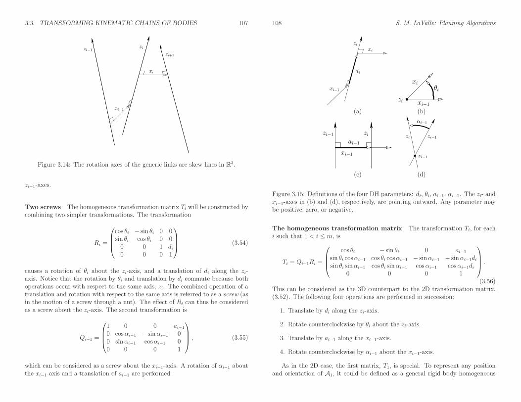
In Section 3.3.1, each Ti was defined in terms of two parameters, ai−1 and θi.For the 3D case, four parameters will be defined: di, θi, ai−1, and αi−1. Theseare referred to as Denavit-Hartenberg (DH) parameters [223]. The definition ofeach parameter is indicated in Figure 3.15. Figure 3.15a shows the definition ofdi. Note that the xi−1- and xi-axes contact the zi-axis at two different places. Letdi denote signed distance between these points of contact. If the xi-axis is abovethe xi−1-axis along the zi-axis, then di is positive; otherwise, di is negative. Theparameter θi is the angle between the xi- and xi−1-axes, which corresponds to therotation about the zi-axis that moves the xi−1-axis to coincide with the xi-axis.The parameter ai is the distance between the zi- and zi−1-axes; recall these aregenerally skew lines in R3. The parameter αi−1 is the angle between the zi- and
3.3. TRANSFORMING KINEMATIC CHAINS OF BODIES 107
zi+1
xi
zi
xi−1
zi−1
Figure 3.14: The rotation axes of the generic links are skew lines in R3.
zi−1-axes.
Two screws The homogeneous transformation matrix Ti will be constructed bycombining two simpler transformations. The transformation
Ri =
cos θi − sin θi 0 0sin θi cos θi 0 00 0 1 di0 0 0 1
(3.54)
causes a rotation of θi about the zi-axis, and a translation of di along the zi-axis. Notice that the rotation by θi and translation by di commute because bothoperations occur with respect to the same axis, zi. The combined operation of atranslation and rotation with respect to the same axis is referred to as a screw (asin the motion of a screw through a nut). The effect of Ri can thus be consideredas a screw about the zi-axis. The second transformation is
Qi−1 =
1 0 0 ai−1
0 cosαi−1 − sinαi−1 00 sinαi−1 cosαi−1 00 0 0 1
, (3.55)
which can be considered as a screw about the xi−1-axis. A rotation of αi−1 aboutthe xi−1-axis and a translation of ai−1 are performed.
108 S. M. LaValle: Planning Algorithms
xi
xi−1
di
zi
θi
xi
zi xi−1
(a) (b)
ai−1
zi−1 zi
xi−1
αi−1
xi−1
zi−1zi
(c) (d)
Figure 3.15: Definitions of the four DH parameters: di, θi, ai−1, αi−1. The zi- andxi−1-axes in (b) and (d), respectively, are pointing outward. Any parameter maybe positive, zero, or negative.
The homogeneous transformation matrix The transformation Ti, for eachi such that 1 < i ≤ m, is
Ti = Qi−1Ri =
cos θi − sin θi 0 ai−1
sin θi cosαi−1 cos θi cosαi−1 − sinαi−1 − sinαi−1disin θi sinαi−1 cos θi sinαi−1 cosαi−1 cosαi−1di
0 0 0 1
.
(3.56)This can be considered as the 3D counterpart to the 2D transformation matrix,(3.52). The following four operations are performed in succession:
1. Translate by di along the zi-axis.
2. Rotate counterclockwise by θi about the zi-axis.
3. Translate by ai−1 along the xi−1-axis.
4. Rotate counterclockwise by αi−1 about the xi−1-axis.
As in the 2D case, the first matrix, T1, is special. To represent any positionand orientation of A1, it could be defined as a general rigid-body homogeneous

3.3. TRANSFORMING KINEMATIC CHAINS OF BODIES 109
x ,1 0
x
z ,1 0
z
x2
y2
x , , x64 5
x
z , y , y65 4
z ,4 6
z
z3
x3y
3
d2
a2
d4
d3
a3
y , y1 0
z2
y5
Figure 3.16: The Puma 560 is shown along with the DH parameters and bodyframes for each link in the chain. This figure is borrowed from [291] by courtesyof the authors.
transformation matrix, (3.50). If the first body is only capable of rotation viaa revolute joint, then a simple convention is usually followed. Let the a0, α0
parameters of T1 be assigned as a0 = α0 = 0 (there is no z0-axis). This impliesthat Q0 from (3.55) is the identity matrix, which makes T1 = R1.
The transformation Ti for i > 1 gives the relationship between the body frameof Ai and the body frame of Ai−1. The position of a point (x, y, z) on Am is givenby
T1T2 · · ·Tm
xyz1
. (3.57)
For each revolute joint, θi is treated as the only variable in Ti. Prismatic jointscan be modeled by allowing ai to vary. More complicated joints can be modeled asa sequence of degenerate joints. For example, a spherical joint can be consideredas a sequence of three zero-length revolute joints; the joints perform a roll, apitch, and a yaw. Another option for more complicated joints is to abandon theDH representation and directly develop the homogeneous transformation matrix.This might be needed to preserve topological properties that become importantin Chapter 4.
Example 3.4 (Puma 560) This example demonstrates the 3D chain kinemat-ics on a classic robot manipulator, the PUMA 560, shown in Figure 3.16. The
110 S. M. LaValle: Planning Algorithms
Matrix αi−1 ai−1 θi di
T1(θ1) 0 0 θ1 0T2(θ2) −π/2 0 θ2 d2T3(θ3) 0 a2 θ3 d3T4(θ4) π/2 a3 θ4 d4T5(θ5) −π/2 0 θ5 0T6(θ6) π/2 0 θ6 0
Figure 3.17: The DH parameters are shown for substitution into each homoge-neous transformation matrix (3.56). Note that a3 and d3 are negative in thisexample (they are signed displacements, not distances).
current parameterization here is based on [29, 291]. The procedure is to determineappropriate body frames to represent each of the links. The first three links allowthe hand (called an end-effector) to make large movements in W , and the lastthree enable the hand to achieve a desired orientation. There are six degrees offreedom, each of which arises from a revolute joint. The body frames are shownin Figure 3.16, and the corresponding DH parameters are given in Figure 3.17.Each transformation matrix Ti is a function of θi; hence, it is written Ti(θi). Theother parameters are fixed for this example. Only θ1, θ2, . . ., θ6 are allowed tovary.
The parameters from Figure 3.17 may be substituted into the homogeneoustransformation matrices to obtain
T1(θ1) =
cos θ1 − sin θ1 0 0sin θ1 cos θ1 0 00 0 1 00 0 0 1
, (3.58)
T2(θ2) =
cos θ2 − sin θ2 0 00 0 1 d2
− sin θ2 − cos θ2 0 00 0 0 1
, (3.59)
T3(θ3) =
cos θ3 − sin θ3 0 a2sin θ3 cos θ3 0 00 0 1 d30 0 0 1
, (3.60)
T4(θ4) =
cos θ4 − sin θ4 0 a30 0 −1 −d4
sin θ4 cos θ4 0 00 0 0 1
, (3.61)
3.3. TRANSFORMING KINEMATIC CHAINS OF BODIES 111
Figure 3.18: A hydrocarbon (octane) molecule with 8 carbon atoms and 18 hy-drogen atoms (courtesy of the New York University MathMol Library).
T5(θ5) =
cos θ5 − sin θ5 0 00 0 1 0
− sin θ5 − cos θ5 0 00 0 0 1
, (3.62)
and
T6(θ6) =
cos θ6 − sin θ6 0 00 0 −1 0
sin θ6 cos θ6 0 00 0 0 1
. (3.63)
A point (x, y, z) in the body frame of the last link A6 appears in W as
T1(θ1)T2(θ2)T3(θ3)T4(θ4)T5(θ5)T6(θ6)
xyz1
. (3.64)
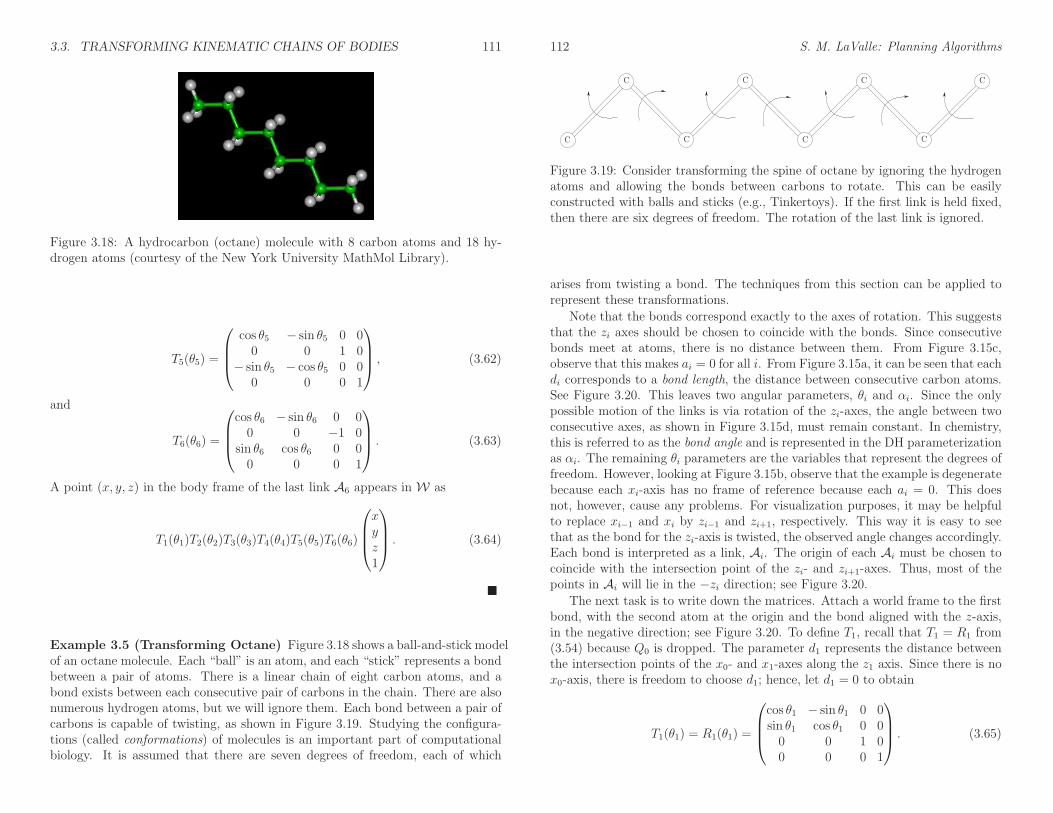
Example 3.5 (Transforming Octane) Figure 3.18 shows a ball-and-stick modelof an octane molecule. Each “ball” is an atom, and each “stick” represents a bondbetween a pair of atoms. There is a linear chain of eight carbon atoms, and abond exists between each consecutive pair of carbons in the chain. There are alsonumerous hydrogen atoms, but we will ignore them. Each bond between a pair ofcarbons is capable of twisting, as shown in Figure 3.19. Studying the configura-tions (called conformations) of molecules is an important part of computationalbiology. It is assumed that there are seven degrees of freedom, each of which
112 S. M. LaValle: Planning Algorithms
C
C
C
C
C
C
C
C
Figure 3.19: Consider transforming the spine of octane by ignoring the hydrogenatoms and allowing the bonds between carbons to rotate. This can be easilyconstructed with balls and sticks (e.g., Tinkertoys). If the first link is held fixed,then there are six degrees of freedom. The rotation of the last link is ignored.
arises from twisting a bond. The techniques from this section can be applied torepresent these transformations.
Note that the bonds correspond exactly to the axes of rotation. This suggeststhat the zi axes should be chosen to coincide with the bonds. Since consecutivebonds meet at atoms, there is no distance between them. From Figure 3.15c,observe that this makes ai = 0 for all i. From Figure 3.15a, it can be seen that eachdi corresponds to a bond length, the distance between consecutive carbon atoms.See Figure 3.20. This leaves two angular parameters, θi and αi. Since the onlypossible motion of the links is via rotation of the zi-axes, the angle between twoconsecutive axes, as shown in Figure 3.15d, must remain constant. In chemistry,this is referred to as the bond angle and is represented in the DH parameterizationas αi. The remaining θi parameters are the variables that represent the degrees offreedom. However, looking at Figure 3.15b, observe that the example is degeneratebecause each xi-axis has no frame of reference because each ai = 0. This doesnot, however, cause any problems. For visualization purposes, it may be helpfulto replace xi−1 and xi by zi−1 and zi+1, respectively. This way it is easy to seethat as the bond for the zi-axis is twisted, the observed angle changes accordingly.Each bond is interpreted as a link, Ai. The origin of each Ai must be chosen tocoincide with the intersection point of the zi- and zi+1-axes. Thus, most of thepoints in Ai will lie in the −zi direction; see Figure 3.20.
The next task is to write down the matrices. Attach a world frame to the firstbond, with the second atom at the origin and the bond aligned with the z-axis,in the negative direction; see Figure 3.20. To define T1, recall that T1 = R1 from(3.54) because Q0 is dropped. The parameter d1 represents the distance betweenthe intersection points of the x0- and x1-axes along the z1 axis. Since there is nox0-axis, there is freedom to choose d1; hence, let d1 = 0 to obtain
T1(θ1) = R1(θ1) =
cos θ1 − sin θ1 0 0sin θ1 cos θ1 0 00 0 1 00 0 0 1
. (3.65)

3.4. TRANSFORMING KINEMATIC TREES 113
zi+1
zi
zi−1
di
Ai
xi
xi−1
Figure 3.20: Each bond may be interpreted as a “link” of length di that is alignedwith the zi-axis. Note that most of Ai appears in the −zi direction.
The application of T1 to points in A1 causes them to rotate around the z1-axis,which appears correct.
The matrices for the remaining six bonds are
Ti(θi) =
cos θi − sin θi 0 0sin θi cosαi−1 cos θi cosαi−1 − sinαi−1 − sinαi−1disin θi sinαi−1 cos θi sinαi−1 cosαi−1 cosαi−1di
0 0 0 1
, (3.66)
for i ∈ 2, . . . , 7. The position of any point, (x, y, z) ∈ A7, is given by
T1(θ1)T2(θ2)T3(θ3)T4(θ4)T5(θ5)T6(θ6)T7(θ7)
xyz1
. (3.67)
3.4 Transforming Kinematic Trees
Motivation For many interesting problems, the linkage is arranged in a “tree”as shown in Figure 3.21a. Assume here that the links are not attached in ways that
114 S. M. LaValle: Planning Algorithms
(a) (b)
Figure 3.21: General linkages: (a) Instead of a chain of rigid bodies, a “tree” ofrigid bodies can be considered. (b) If there are loops, then parameters must becarefully assigned to ensure that the loops are closed.
form loops (i.e., Figure 3.21b); that case is deferred until Section 4.4, althoughsome comments are also made at the end of this section. The human body, with itsjoints and limbs attached to the torso, is an example that can be modeled as a treeof rigid links. Joints such as knees and elbows are considered as revolute joints.A shoulder joint is an example of a spherical joint, although it cannot achieve anyorientation (without a visit to the emergency room!). As mentioned in Section1.4, there is widespread interest in animating humans in virtual environments andalso in developing humanoid robots. Both of these cases rely on formulations ofkinematics that mimic the human body.
Another problem that involves kinematic trees is the conformational analysis ofmolecules. Example 3.5 involved a single chain; however, most organic moleculesare more complicated, as in the familiar drugs shown in Figure 1.14a (Section 1.2).The bonds may twist to give degrees of freedom to the molecule. Moving throughthe space of conformations requires the formulation of a kinematic tree. Studyingthese conformations is important because scientists need to determine for somecandidate drug whether the molecule can twist the right way so that it docksnicely (i.e., requires low energy) with a protein cavity; this induces a pharmaco-logical effect, which hopefully is the desired one. Another important problem isdetermining how complicated protein molecules fold into certain configurations.These molecules are orders of magnitude larger (in terms of numbers of atomsand degrees of freedom) than typical drug molecules. For more information, seeSection 7.5.

3.4. TRANSFORMING KINEMATIC TREES 115
A6A7
A13
A8
A9
A12
A5
Figure 3.22: Now it is possible for a link to have more than two joints, as in A7.
Common joints for W = R2 First consider the simplest case in which there isa 2D tree of links for which every link has only two points at which revolute jointsmay be attached. This corresponds to Figure 3.21a. A single link is designated asthe root, A1, of the tree. To determine the transformation of a body, Ai, in thetree, the tools from Section 3.3.1 are directly applied to the chain of bodies thatconnects Ai to A1 while ignoring all other bodies. Each link contributes a θi tothe total degrees of freedom of the tree. This case seems quite straightforward;unfortunately, it is not this easy in general.
Junctions with more than two rotation axes Now consider modeling amore complicated collection of attached links. The main novelty is that one linkmay have joints attached to it in more than two locations, as in A7 in Figure 3.22.A link with more than two joints will be referred to as a junction.
If there is only one junction, then most of the complications arising fromjunctions can be avoided by choosing the junction as the root. For example, fora simple humanoid model, the torso would be a junction. It would be sensibleto make this the root of the tree, as opposed to the right foot. The legs, arms,and head could all be modeled as independent chains. In each chain, the onlyconcern is that the first link of each chain does not attach to the same point onthe torso. This can be solved by inserting a fixed, fictitious link that connectsfrom the origin of the torso to the attachment point of the limb.
The situation is more interesting if there are multiple junctions. Suppose thatFigure 3.22 represents part of a 2D system of links for which the root, A1, isattached via a chain of links to A5. To transform link A9, the tools from Section
116 S. M. LaValle: Planning Algorithms
A7
y7y7
x7
x7
φ
Figure 3.23: The junction is assigned two different frames, depending on whichchain was followed. The solid axes were obtained from transforming A9, and thedashed axes were obtained from transforming A13.
3.3.1 may be directly applied to yield a sequence of transformations,
T1 · · ·T5T6T7T8T9
xy1
, (3.68)
for a point (x, y) ∈ A9. Likewise, to transform T13, the sequence
T1 · · ·T5T6T7T12T13
xy1
(3.69)
can be used by ignoring the chain formed by A8 and A9. So far everything seemsto work well, but take a close look at A7. As shown in Figure 3.23, its body framewas defined in two different ways, one for each chain. If both are forced to usethe same frame, then at least one must abandon the nice conventions of Section3.3.1 for choosing frames. This situation becomes worse for 3D trees becausethis would suggest abandoning the DH parameterization. The Khalil-Kleinfingerparameterization is an elegant extension of the DH parameterization and solvesthese frame assignment issues [272].
Constraining parameters Fortunately, it is fine to use different frames whenfollowing different chains; however, one extra piece of information is needed. Imag-

3.4. TRANSFORMING KINEMATIC TREES 117
ine transforming the whole tree. The variable θ7 will appear twice, once from eachof the upper and lower chains. Let θ7u and θ7l denote these θ’s. Can θ really bechosen two different ways? This would imply that the tree is instead as picturedin Figure 3.24, in which there are two independently moving links, A7u and A7l.To fix this problem, a constraint must be imposed. Suppose that θ7l is treated as
A6
A13
A8
A9
A12
A5
A7u
A7l
Figure 3.24: Choosing each θ7 independently would result in a tree that ignoresthat fact that A7 is rigid.
an independent variable. The parameter θ7u must then be chosen as θ7l + φ, inwhich φ is as shown in Figure 3.23.
Example 3.6 (A 2D Tree of Bodies) Figure 3.25 shows a 2D example thatinvolves six links. To transform (x, y) ∈ A6, the only relevant links are A5, A2,and A1. The chain of transformations is
T1T2lT5T6
xy1
, (3.70)
in which
T1 =
cos θ1 − sin θ1 xtsin θ1 cos θ1 yt0 0 1
=
cos θ1 − sin θ1 0sin θ1 cos θ1 00 0 1
, (3.71)
T2l =
cos θ2l − sin θ2l a1sin θ2l cos θ2l 00 0 1
=
cos θ2 − sin θ2 1sin θ2 cos θ2 00 0 1
, (3.72)
T5 =
cos θ5 − sin θ5 a2sin θ5 cos θ5 00 0 1
=
cos θ5 − sin θ5√2
sin θ5 cos θ5 00 0 1
, (3.73)
118 S. M. LaValle: Planning Algorithms
(0,0) (1,0) (3,0) (4,0)
(0,−1)A1
A2
A3
A6
A5
A4
(0, 0) (1, 0) (3, 0)
(2,−1)
(4, 0)
Figure 3.25: A tree of bodies in which the joints are attached in different places.
and
T6 =
cos θ6 − sin θ6 a5sin θ6 cos θ6 00 0 1
=
cos θ6 − sin θ6 1sin θ6 cos θ6 00 0 1
. (3.74)
The matrix T2l in (3.72) denotes the fact that the lower chain was followed. Thetransformation for points in A4 is
T1T2uT4T5
xy1
, (3.75)
in which T1 is the same as in (3.71), and
T3 =
cos θ3 − sin θ3 a2sin θ3 cos θ3 00 0 1
=
cos θ3 − sin θ3√2
sin θ3 cos θ3 00 0 1
, (3.76)
and
T4 =
cos θ4 − sin θ4 a4sin θ4 cos θ4 00 0 1
=
cos θ4 − sin θ4 0sin θ4 cos θ4 00 0 1
. (3.77)
The interesting case is
T2u =
cos θ2u − sin θ2u a1sin θ2u cos θ2u 0
0 0 1
=
cos(θ2l + π/4) − sin(θ2l + π/4) a1sin(θ2l + π/4) cos(θ2l + π/4) 0
0 0 1
,
(3.78)

3.4. TRANSFORMING KINEMATIC TREES 119
A2A3
A4
A5
A7
A10
A9
A1
A8
A6
Figure 3.26: There are ten links and ten revolute joints arranged in a loop. Thisis an example of a closed kinematic chain.
in which the constraint θ2u = θ2l + π/4 is imposed to enforce the fact that A2 isa junction.
For a 3D tree of bodies the same general principles may be followed. In somecases, there will not be any complications that involve special considerations ofjunctions and constraints. One example of this is the transformation of flexiblemolecules because all consecutive rotation axes intersect, and junctions occurdirectly at these points of intersection. In general, however, the DH parametertechnique may be applied for each chain, and then the appropriate constraintshave to be determined and applied to represent the true degrees of freedom of thetree. The Khalil-Kleinfinger parameterization conveniently captures the resultingsolution [272].
What if there are loops? The most general case includes links that are con-nected in loops, as shown in Figure 3.26. These are generally referred to as closedkinematic chains. This arises in many applications. For example, with humanoidrobotics or digital actors, a loop is formed when both feet touch the ground. Asanother example, suppose that two robot manipulators, such as the Puma 560from Example 3.4, cooperate together to carry an object. If each robot grasps thesame object with its hand, then a loop will be formed. A complicated exampleof this was shown in Figure 1.5, in which mobile robots moved a piano. Outsideof robotics, a large fraction of organic molecules have flexible loops. Exploringthe space of their conformations requires careful consideration of the difficultiesimposed by these loops.
The main difficulty of working with closed kinematic chains is that it is hardto determine which parameter values are within an acceptable range to ensureclosure. If these values are given, then the transformations are handled in the
120 S. M. LaValle: Planning Algorithms
A7
A10
A9A8
A6
A1
A2
A5
A4
A3
Figure 3.27: Loops may be opened to enable tree-based transformations to beapplied; however, a closure constraint must still be satisfied.
same way as the case of trees. For example, the links in Figure 3.26 may betransformed by breaking the loop into two different chains. Suppose we forgetthat the joint between A5 and A6 exists, as shown in Figure 3.27. Consider twodifferent kinematic chains that start at the joint on the extreme left. There is anupper chain from A1 to A5 and a lower chain from A10 to A6. The transformationsfor any of these bodies can be obtained directly from the techniques of Section3.3.1. Thus, it is easy to transform the bodies, but how do we choose parametervalues that ensure A5 and A6 are connected at their common joint? Using theupper chain, the position of this joint may be expressed as
T1(θ1)T2(θ2)T3(θ3)T4(θ4)T5(θ5)
a501
, (3.79)
in which (a5, 0) ∈ A5 is the location of the joint of A5 that is supposed to connectto A6. The position of this joint may also be expressed using the lower chain as
T10(θ10)T9(θ9)T8(θ8)T7(θ7)T6(θ6)
a601
, (3.80)
with (a6, 0) representing the position of the joint in the body frame of A6. Ifthe loop does not have to be maintained, then any values for θ1, . . ., θ10 may beselected, resulting in ten degrees of freedom. However, if a loop must maintained,
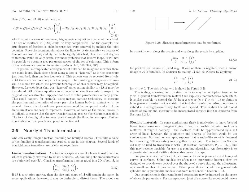
3.5. NONRIGID TRANSFORMATIONS 121
then (3.79) and (3.80) must be equal,
T1(θ1)T2(θ2)T3(θ3)T4(θ4)T5(θ5)
a501
= T10(θ10)T9(θ9)T8(θ8)T7(θ7)T6(θ6)
a601
,
(3.81)which is quite a mess of nonlinear, trigonometric equations that must be solved.The set of solutions to (3.81) could be very complicated. For the example, thetrue degrees of freedom is eight because two were removed by making the jointcommon. Since the common joint allows the links to rotate, exactly two degrees offreedom are lost. If A5 and A6 had to be rigidly attached, then the total degreesof freedom would be only seven. For most problems that involve loops, it will notbe possible to obtain a nice parameterization of the set of solutions. This a formof the well-known inverse kinematics problem [140, 360, 395, 485].
In general, a complicated arrangement of links can be imagined in which thereare many loops. Each time a joint along a loop is “ignored,” as in the procedurejust described, then one less loop exists. This process can be repeated iterativelyuntil there are no more loops in the graph. The resulting arrangement of linkswill be a tree for which the previous techniques of this section may be applied.However, for each joint that was “ignored” an equation similar to (3.81) must beintroduced. All of these equations must be satisfied simultaneously to respect theoriginal loop constraints. Suppose that a set of value parameters is already given.This could happen, for example, using motion capture technology to measurethe position and orientation of every part of a human body in contact with theground. From this the solution parameters could be computed, and all of thetransformations are easy to represent. However, as soon as the model moves, itis difficult to ensure that the new transformations respect the closure constraints.The foot of the digital actor may push through the floor, for example. Furtherinformation on this problem appears in Section 4.4.
3.5 Nonrigid Transformations
One can easily imagine motion planning for nonrigid bodies. This falls outsideof the families of transformations studied so far in this chapter. Several kinds ofnonrigid transformations are briefly surveyed here.
Linear transformations A rotation is a special case of a linear transformation,which is generally expressed by an n×n matrix,M , assuming the transformationsare performed over Rn. Consider transforming a point (x, y) in a 2D robot, A, as
(
m11 m12
m21 m22
)(
xy
)
. (3.82)
If M is a rotation matrix, then the size and shape of A will remain the same. Insome applications, however, it may be desirable to distort these. The robot can
122 S. M. LaValle: Planning Algorithms
Figure 3.28: Shearing transformations may be performed.
be scaled by m11 along the x-axis and m22 along the y-axis by applying
(
m11 00 m22
)(
xy
)
, (3.83)
for positive real values m11 and m22. If one of them is negated, then a mirrorimage of A is obtained. In addition to scaling, A can be sheared by applying
(
1 m12
0 1
)(
xy
)
(3.84)
for m12 6= 0. The case of m12 = 1 is shown in Figure 3.28.The scaling, shearing, and rotation matrices may be multiplied together to
yield a general transformation matrix that explicitly parameterizes each effect.It is also possible to extend the M from n × n to (n + 1) × (n + 1) to obtain ahomogeneous transformation matrix that includes translation. Also, the conceptsextend in a straightforward way to R3 and beyond. This enables the additionaleffects of scaling and shearing to be incorporated directly into the concepts fromSections 3.2-3.4.
Flexible materials In some applications there is motivation to move beyondlinear transformations. Imagine trying to warp a flexible material, such as amattress, through a doorway. The mattress could be approximated by a 2Darray of links; however, the complexity and degrees of freedom would be toocumbersome. For another example, suppose that a snake-like robot is designedby connecting 100 revolute joints together in a chain. The tools from Section3.3 may be used to transform it with 100 rotation parameters, θ1, . . ., θ100, butthis may become unwieldy for use in a planning algorithm. An alternative is toapproximate the snake with a deformable curve or shape.
For problems such as these, it is desirable to use a parameterized family ofcurves or surfaces. Spline models are often most appropriate because they aredesigned to provide easy control over the shape of a curve through the adjustmentof a small number of parameters. Other possibilities include the generalized-cylinder and superquadric models that were mentioned in Section 3.1.3.
One complication is that complicated constraints may be imposed on the spaceof allowable parameters. For example, each joint of a snake-like robot could have a
3.5. NONRIGID TRANSFORMATIONS 123
small range of rotation. This would be easy to model using a kinematic chain; how-ever, determining which splines from a spline family satisfy this extra constraintmay be difficult. Likewise, for manipulating flexible materials, there are usuallycomplicated constraints based on the elasticity of the material. Even determiningits correct shape under the application of some forces requires integration of anelastic energy function over the material [300].
Further Reading
Section 3.1 barely scratches the surface of geometric modeling. Most literature focuseson parametric curves and surfaces [190, 374, 399]. These models are not as popularfor motion planning because obtaining efficient collision detection is most importantin practice, and processing implicit algebraic surfaces is most important in theoreticalmethods. A thorough coverage of solid and boundary representations, including semi-algebraic models, can be found in [234]. Theoretical algorithm issues regarding semi-algebraic models are covered in [369, 370]. For a comparison of the doubly connectededge list to its variants, see [270].
The material of Section 3.2 appears in virtually any book on robotics, computer vi-sion, or computer graphics. Consulting linear algebra texts may be helpful to gain moreinsight into rotations. There are many ways to parameterize the set of all 3D rotationmatrices. The yaw-pitch-roll formulation was selected because it is the easiest to under-stand. There are generally 12 different variants of the yaw-pitch-roll formulation (alsocalled Euler angles) based on different rotation orderings and axis selections. This for-mulation, however, is not well suited for the development of motion planning algorithms.It is easy (and safe) to use for making quick 3D animations of motion planning out-put, but it incorrectly captures the structure of the state space for planning algorithms.Section 4.2 introduces the quaternion parameterization, which correctly captures thisstate space; however, it is harder to interpret when constructing examples. Therefore,it is helpful to understand both. In addition to Euler angles and quaternions, there isstill motivation for using many other parameterizations of rotations, such as sphericalcoordinates, Cayley-Rodrigues parameters, and stereographic projection. Chapter 5 of[113] provides extensive coverage of 3D rotations and different parameterizations.
The coverage in Section 3.3 of transformations of chains of bodies was heavily influ-enced by two classic robotics texts [140, 395]. The DH parameters were introduced in[223] and later extended to trees and loops in [272]. An alternative to DH parameters isexponential coordinates [378], which simplify some computations; however, determiningthe parameters in the modeling stage may be less intuitive. A fascinating history ofmechanisms appears in [224]. Other texts on kinematics include [23, 163, 277, 359].The standard approach in many robotics books [184, 432, 447, 485] is to introduce thekinematic chain formulations and DH parameters in the first couple of chapters, andthen move on to topics that are crucial for controlling robot manipulators, includingdynamics modeling, singularities, manipulability, and control. Since this book is con-cerned instead with planning algorithms, we depart at the point where dynamics wouldusually be covered and move into a careful study of the configuration space in Chapter4.
124 S. M. LaValle: Planning Algorithms
Exercises
1. Define a semi-algebraic model that removes a triangular “nose” from the regionshown in Figure 3.4.
2. For distinct values of yaw, pitch, and roll, it is possible to generate the samerotation. In other words, R(α, β, γ) = R(α′, β′, γ′) for some cases in which atleast α 6= α, β 6= β′, or γ 6= γ′. Characterize the sets of angles for which thisoccurs.
3. Using rotation matrices, prove that 2D rotation is commutative but 3D rotationis not.
4. An alternative to the yaw-pitch-roll formulation from Section 3.2.3 is consideredhere. Consider the following Euler angle representation of rotation (there aremany other variants). The first rotation is Rz(γ), which is just (3.39) with αreplaced by γ. The next two rotations are identical to the yaw-pitch-roll for-mulation: Ry(β) is applied, followed by Rz(α). This yields Reuler(α, β, γ) =Rz(α)Ry(β)Rz(γ).
(a) Determine the matrix Reuler.
(b) Show that Reuler(α, β, γ) = Reuler(α− π,−β, γ − π).
(c) Suppose that a rotation matrix is given as shown in (3.43). Show that theEuler angles are
α = atan2(r23, r13), (3.85)
β = atan2(√
1− r233, r33), (3.86)
and
γ = atan2(r32,−r31). (3.87)
5. There are 12 different variants of yaw-pitch-roll (or Euler angles), depending onwhich axes are used and the order of these axes. Determine all of the possibilities,using only notation such as Rz(α)Ry(β)Rz(γ) for each one. Give brief argumentsthat support why or why not specific combinations of rotations are included inyour list of 12.
6. Let A be a unit disc, centered at the origin, and W = R2. Assume that A isrepresented by a single, algebraic primitive, H = (x, y) | x2 + y2 ≤ 1. Showthat the transformed primitive is unchanged after any rotation is applied.
7. Consider the articulated chain of bodies shown in Figure 3.29. There are threeidentical rectangular bars in the plane, called A1,A2,A3. Each bar has width 2and length 12. The distance between the two points of attachment is 10. Thefirst bar, A1, is attached to the origin. The second bar, A2, is attached to A1,and A3 is attached to A2. Each bar is allowed to rotate about its point ofattachment. The configuration of the chain can be expressed with three angles,

3.5. NONRIGID TRANSFORMATIONS 125
(0,0)
2
10
a
b
c
12
A1A2
A3
Figure 3.29: A chain of three bodies.
(0,0) (1,0) (3,0) (4,0)A2
A1 A3
Figure 3.30: Another exercise involving a chain of bodies.
(θ1, θ2, θ3). The first angle, θ1, represents the angle between the segment drawnbetween the two points of attachment of A1 and the x-axis. The second angle, θ2,represents the angle betweenA2 andA1 (θ2 = 0 when they are parallel). The thirdangle, θ3, represents the angle between A3 and A2. Suppose the configuration is(π/4, π/2,−π/4).
(a) Use the homogeneous transformation matrices to determine the locations ofpoints a, b, and c.
(b) Characterize the set of all configurations for which the final point of attach-ment (near the end of A3) is at (0, 0) (you should be able to figure this outwithout using the matrices).
8. A three-link chain of bodies that moves in a 2D world is shown Figure 3.30. Thefirst link, A1, is attached at (0, 0) but can rotate. Each remaining link is attachedto another link with a revolute joint. The second link, A2, is a rigid ring, and theother two links are rectangular bars.
Assume that the structure is shown in the zero configuration. Suppose thatthe linkage is moved to the configuration (θ1, θ2, θ3) = (π4 ,
π2 ,
π4 ), in which θ1 is
the angle of A1, θ2 is the angle of A2 with respect to A1, and θ3 is the angle of A3
with respect to A2. Using homogeneous transformation matrices, compute theposition of the point at (4, 0) in Figure 3.30, when the linkage is at configuration(π4 ,
π2 ,
π4 ) (the point is attached to A3).
126 S. M. LaValle: Planning Algorithms
9. Approximate a spherical joint as a chain of three short, perpendicular links thatare attached by revolute joints and give the sequence of transformation matrices.Show that as the link lengths approach zero, the resulting sequence of trans-formation matrices converges to exactly representing the freedom of a sphericaljoint. Compare this approach to directly using a full rotation matrix, (3.42), torepresent the joint in the homogeneous transformation matrix.
10. Figure 3.12 showed six different ways in which 2D surfaces can slide with respectto each other to produce a joint.
(a) Suppose that two bodies contact each other along a one-dimensional curve.Characterize as many different kinds of “joints” as possible, and indicatethe degrees of freedom of each.
(b) Suppose that the two bodies contact each other at a point. Indicate the typesof rolling and sliding that are possible, and their corresponding degrees offreedom.
11. Suppose that two bodies form a screw joint in which the axis of the central axisof the screw aligns with the x-axis of the first body. Determine an appropriatehomogeneous transformation matrix to use in place of the DH matrix. Define thematrix with the screw radius, r, and displacement-per-revolution, d, as parame-ters.
12. Recall Example 3.6. How should the transformations be modified so that thelinks are in the positions shown in Figure 3.25 at the zero configuration (θi = 0for every revolute joint whose angle can be independently chosen)?
13. Generalize the shearing transformation of (3.84) to enable shearing of 3D models.
Implementations
14. Develop and implement a kinematic model for 2D linkages. Enable the user todisplay the arrangement of links in the plane.
15. Implement the kinematics of molecules that do not have loops and show themgraphically as a “ball and stick” model. The user should be able to input theatomic radii, bond connections, bond lengths, and rotation ranges for each bond.
16. Design and implement a software system in which the user can interactively attachvarious links to make linkages that resemble those possible from using Tinkertoys(or another popular construction set that allows pieces to move). There are severalrods of various lengths, which fit into holes in the center and around the edge ofseveral coin-shaped pieces. Assume that all joints are revolute. The user shouldbe allowed to change parameters and see the resulting positions of all of the links.
17. Construct a model of the human body as a tree of links in a 3D world. Forsimplicity, the geometric model may be limited to spheres and cylinders. Designand implement a system that displays the virtual human and allows the user toclick on joints of the body to enable them to rotate.

3.5. NONRIGID TRANSFORMATIONS 127
18. Develop a simulator with 3D graphics for the Puma 560 model shown in Figure3.4.
128 S. M. LaValle: Planning Algorithms
Chapter 4
The Configuration Space
Chapter 3 only covered how to model and transform a collection of bodies; how-ever, for the purposes of planning it is important to define the state space. Thestate space for motion planning is a set of possible transformations that could beapplied to the robot. This will be referred to as the configuration space, based onLagrangian mechanics and the seminal work of Lozano-Perez [343, 347, 344], whoextensively utilized this notion in the context of planning (the idea was also usedin early collision avoidance work by Udupa [462]). The motion planning litera-ture was further unified around this concept by Latombe’s book [304]. Once theconfiguration space is clearly understood, many motion planning problems thatappear different in terms of geometry and kinematics can be solved by the sameplanning algorithms. This level of abstraction is therefore very important.
This chapter provides important foundational material that will be very usefulin Chapters 5 to 8 and other places where planning over continuous state spacesoccurs. Many concepts introduced in this chapter come directly from mathemat-ics, particularly from topology. Therefore, Section 4.1 gives a basic overview oftopological concepts. Section 4.2 uses the concepts from Chapter 3 to define theconfiguration space. After reading this, you should be able to precisely character-ize the configuration space of a robot and understand its structure. In Section 4.3,obstacles in the world are transformed into obstacles in the configuration space,but it is important to understand that this transformation may not be explicitlyconstructed. The implicit representation of the state space is a recurring themethroughout planning. Section 4.4 covers the important case of kinematic chainsthat have loops, which was mentioned in Section 3.4. This case is so difficult thateven the space of transformations usually cannot be explicitly characterized (i.e.,parameterized).
4.1 Basic Topological Concepts
This section introduces basic topological concepts that are helpful in understand-ing configuration spaces. Topology is a challenging subject to understand in depth.
129
130 S. M. LaValle: Planning Algorithms
The treatment given here provides only a brief overview and is designed to stim-ulate further study (see the literature overview at the end of the chapter). Toadvance further in this chapter, it is not necessary to understand all of the ma-terial of this section; however, the more you understand, the deeper will be yourunderstanding of motion planning in general.
4.1.1 Topological Spaces
Recall the concepts of open and closed intervals in the set of real numbers R. Theopen interval (0, 1) includes all real numbers between 0 and 1, except 0 and 1.However, for either endpoint, an infinite sequence may be defined that convergesto it. For example, the sequence 1/2, 1/4, . . ., 1/2i converges to 0 as i tendsto infinity. This means that we can choose a point in (0, 1) within any small,positive distance from 0 or 1, but we cannot pick one exactly on the boundary ofthe interval. For a closed interval, such as [0, 1], the boundary points are included.
The notion of an open set lies at the heart of topology. The open set definitionthat will appear here is a substantial generalization of the concept of an openinterval. The concept applies to a very general collection of subsets of some largerspace. It is general enough to easily include any kind of configuration space thatmay be encountered in planning.
A set X is called a topological space if there is a collection of subsets of Xcalled open sets for which the following axioms hold:
1. The union of any number of open sets is an open set.
2. The intersection of a finite number of open sets is an open set.
3. Both X and ∅ are open sets.
Note that in the first axiom, the union of an infinite number of open sets may betaken, and the result must remain an open set. Intersecting an infinite number ofopen sets, however, does not necessarily lead to an open set.
For the special case of X = R, the open sets include open intervals, as ex-pected. Many sets that are not intervals are open sets because taking unions andintersections of open intervals yields other open sets. For example, the set
∞⋃
i=1
(
1
3i,2
3i
)
, (4.1)
which is an infinite union of pairwise-disjoint intervals, is an open set.
Closed sets Open sets appear directly in the definition of a topological space.It next seems that closed sets are needed. Suppose X is a topological space.A subset C ⊂ X is defined to be a closed set if and only if X \ C is an openset. Thus, the complement of any open set is closed, and the complement of any
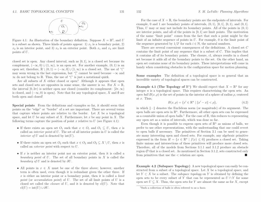
4.1. BASIC TOPOLOGICAL CONCEPTS 131
x1
U
x3
x2
O2
O1
Figure 4.1: An illustration of the boundary definition. Suppose X = R2, and Uis a subset as shown. Three kinds of points appear: 1) x1 is a boundary point, 2)x2 is an interior point, and 3) x3 is an exterior point. Both x1 and x2 are limitpoints of U .
closed set is open. Any closed interval, such as [0, 1], is a closed set because itscomplement, (−∞, 0) ∪ (1,∞), is an open set. For another example, (0, 1) is anopen set; therefore, R \ (0, 1) = (−∞, 0] ∪ [1,∞) is a closed set. The use of “(”may seem wrong in the last expression, but “[” cannot be used because −∞ and∞ do not belong to R. Thus, the use of “(” is just a notational quirk.
Are all subsets of X either closed or open? Although it appears that opensets and closed sets are opposites in some sense, the answer is no. For X = R,the interval [0, 2π) is neither open nor closed (consider its complement: [2π,∞)is closed, and (−∞, 0) is open). Note that for any topological space, X and ∅ areboth open and closed!
Special points From the definitions and examples so far, it should seem thatpoints on the “edge” or “border” of a set are important. There are several termsthat capture where points are relative to the border. Let X be a topologicalspace, and let U be any subset of X. Furthermore, let x be any point in X. Thefollowing terms capture the position of point x relative to U (see Figure 4.1):
• If there exists an open set O1 such that x ∈ O1 and O1 ⊆ U , then x iscalled an interior point of U . The set of all interior points in U is called theinterior of U and is denoted by int(U).
• If there exists an open set O2 such that x ∈ O2 and O2 ⊆ X \ U , then x iscalled an exterior point with respect to U .
• If x is neither an interior point nor an exterior point, then it is called aboundary point of U . The set of all boundary points in X is called theboundary of U and is denoted by ∂U .
• All points in x ∈ X must be one of the three above; however, anotherterm is often used, even though it is redundant given the other three. Ifx is either an interior point or a boundary point, then it is called a limitpoint (or accumulation point) of U . The set of all limit points of U is aclosed set called the closure of U , and it is denoted by cl(U). Note thatcl(U) = int(U) ∪ ∂U .
132 S. M. LaValle: Planning Algorithms
For the case of X = R, the boundary points are the endpoints of intervals. Forexample, 0 and 1 are boundary points of intervals, (0, 1), [0, 1], [0, 1), and (0, 1].Thus, U may or may not include its boundary points. All of the points in (0, 1)are interior points, and all of the points in [0, 1] are limit points. The motivationof the name “limit point” comes from the fact that such a point might be thelimit of an infinite sequence of points in U . For example, 0 is the limit point ofthe sequence generated by 1/2i for each i ∈ N, the natural numbers.
There are several convenient consequences of the definitions. A closed set Ccontains the limit point of any sequence that is a subset of C. This implies thatit contains all of its boundary points. The closure, cl, always results in a closedset because it adds all of the boundary points to the set. On the other hand, anopen set contains none of its boundary points. These interpretations will come inhandy when considering obstacles in the configuration space for motion planning.
Some examples The definition of a topological space is so general that anincredible variety of topological spaces can be constructed.
Example 4.1 (The Topology of Rn) We should expect that X = Rn for anyinteger n is a topological space. This requires characterizing the open sets. Anopen ball B(x, ρ) is the set of points in the interior of a sphere of radius ρ, centeredat x. Thus,
B(x, ρ) = x′ ∈ Rn | ‖x′ − x‖ < ρ, (4.2)
in which ‖ · ‖ denotes the Euclidean norm (or magnitude) of its argument. Theopen balls are open sets in Rn. Furthermore, all other open sets can be expressedas a countable union of open balls.1 For the case of R, this reduces to representingany open set as a union of intervals, which was done so far.
Even though it is possible to express open sets of Rn as unions of balls, weprefer to use other representations, with the understanding that one could revertto open balls if necessary. The primitives of Section 3.1 can be used to gener-ate many interesting open and closed sets. For example, any algebraic primitiveexpressed in the form H = x ∈ Rn | f(x) ≤ 0 produces a closed set. Takingfinite unions and intersections of these primitives will produce more closed sets.Therefore, all of the models from Sections 3.1.1 and 3.1.2 produce an obstacleregion O that is a closed set. As mentioned in Section 3.1.2, sets constructed onlyfrom primitives that use the < relation are open.
Example 4.2 (Subspace Topology) A new topological space can easily be con-structed from a subset of a topological space. Let X be a topological space, andlet Y ⊂ X be a subset. The subspace topology on Y is obtained by defining theopen sets to be every subset of Y that can be represented as U ∩ Y for someopen set U ⊆ X. Thus, the open sets for Y are almost the same as for X, except
1Such a collection of balls is often referred to as a basis.

4.1. BASIC TOPOLOGICAL CONCEPTS 133
that the points that do not lie in Y are trimmed away. New subspaces can beconstructed by intersecting open sets of Rn with a complicated region defined bysemi-algebraic models. This leads to many interesting topological spaces, some ofwhich will appear later in this chapter.
Example 4.3 (The Trivial Topology) For any set X, there is always one triv-ial example of a topological space that can be constructed from it. Declare thatX and ∅ are the only open sets. Note that all of the axioms are satisfied.
Example 4.4 (A Strange Topology) It is important to keep in mind the al-most absurd level of generality that is allowed by the definition of a topologicalspace. A topological space can be defined for any set, as long as the declared opensets obey the axioms. Suppose a four-element set is defined as
X = cat,dog,tree,house. (4.3)
In addition to ∅ and X, suppose that cat and dog are open sets. Using theaxioms, cat,dog must also be an open set. Closed sets and boundary pointscan be derived for this topology once the open sets are defined.
After the last example, it seems that topological spaces are so general that notmuch can be said about them. Most spaces that are considered in topology andanalysis satisfy more axioms. For Rn and any configuration spaces that arise inthis book, the following is satisfied:
Hausdorff axiom: For any distinct x1, x2 ∈ X, there exist open sets O1 andO2 such that x1 ∈ O1, x2 ∈ O2, and O1 ∩O2 = ∅.
In other words, it is possible to separate x1 and x2 into nonoverlapping opensets. Think about how to do this for Rn by selecting small enough open balls. Anytopological space X that satisfies the Hausdorff axiom is referred to as a Hausdorffspace. Section 4.1.2 will introduce manifolds, which happen to be Hausdorff spacesand are general enough to capture the vast majority of configuration spaces thatarise. We will have no need in this book to consider topological spaces that arenot Hausdorff spaces.
Continuous functions A very simple definition of continuity exists for topo-logical spaces. It nicely generalizes the definition from standard calculus. Letf : X → Y denote a function between topological spaces X and Y . For any setB ⊆ Y , let the preimage of B be denoted and defined by
f−1(B) = x ∈ X | f(x) ∈ B. (4.4)
Note that this definition does not require f to have an inverse.
134 S. M. LaValle: Planning Algorithms
The function f is called continuous if f−1(O) is an open set for every open setO ⊆ Y . Analysis is greatly simplified by this definition of continuity. For example,to show that any composition of continuous functions is continuous requires onlya one-line argument that the preimage of the preimage of any open set alwaysyields an open set. Compare this to the cumbersome classical proof that requiresa mess of δ’s and ǫ’s. The notion is also so general that continuous functions caneven be defined on the absurd topological space from Example 4.4.
Homeomorphism: Making a donut into a coffee cup You might haveheard the expression that to a topologist, a donut and a coffee cup appear thesame. In many branches of mathematics, it is important to define when twobasic objects are equivalent. In graph theory (and group theory), this equivalencerelation is called an isomorphism. In topology, the most basic equivalence is ahomeomorphism, which allows spaces that appear quite different in most othersubjects to be declared equivalent in topology. The surfaces of a donut and acoffee cup (with one handle) are considered equivalent because both have a singlehole. This notion needs to be made more precise!
Suppose f : X → Y is a bijective (one-to-one and onto) function betweentopological spaces X and Y . Since f is bijective, the inverse f−1 exists. If bothf and f−1 are continuous, then f is called a homeomorphism. Two topologicalspaces X and Y are said to be homeomorphic, denoted by X ∼= Y , if there exists ahomeomorphism between them. This implies an equivalence relation on the set oftopological spaces (verify that the reflexive, symmetric, and transitive propertiesare implied by the homeomorphism).
Example 4.5 (Interval Homeomorphisms) Any open interval of R is home-omorphic to any other open interval. For example, (0, 1) can be mapped to (0, 5)by the continuous mapping x 7→ 5x. Note that (0, 1) and (0, 5) are each beinginterpreted here as topological subspaces of R. This kind of homeomorphism canbe generalized substantially using linear algebra. If a subset, X ⊂ Rn, can bemapped to another, Y ⊂ Rn, via a nonsingular linear transformation, then Xand Y are homeomorphic. For example, the rigid-body transformations of theprevious chapter were examples of homeomorphisms applied to the robot. Thus,the topology of the robot does not change when it is translated or rotated. (Inthis example, note that the robot itself is the topological space. This will not bethe case for the rest of the chapter.)
Be careful when mixing closed and open sets. The space [0, 1] is not homeomor-phic to (0, 1), and neither is homeomorphic to [0, 1). The endpoints cause troublewhen trying to make a bijective, continuous function. Surprisingly, a bounded andunbounded set may be homeomorphic. A subset X of Rn is called bounded if thereexists a ball B ⊂ Rn such that X ⊂ B. The mapping x 7→ 1/x establishes that(0, 1) and (1,∞) are homeomorphic. The mapping x 7→ 2 tan−1(x)/π establishesthat (−1, 1) and all of R are homeomorphic!

4.1. BASIC TOPOLOGICAL CONCEPTS 135
Figure 4.2: Even though the graphs are not isomorphic, the corresponding topo-logical spaces may be homeomorphic due to useless vertices. The example graphsmap into R2, and are all homeomorphic to a circle.
Figure 4.3: These topological graphs map into subsets of R2 that are not homeo-morphic to each other.
Example 4.6 (Topological Graphs) Let X be a topological space. The pre-vious example can be extended nicely to make homeomorphisms look like graphisomorphisms. Let a topological graph2 be a graph for which every vertex cor-responds to a point in X and every edge corresponds to a continuous, injective(one-to-one) function, τ : [0, 1] → X. The image of τ connects the points in Xthat correspond to the endpoints (vertices) of the edge. The images of differentedge functions are not allowed to intersect, except at vertices. Recall from graphtheory that two graphs, G1(V1, E1) and G2(V2, E2), are called isomorphic if thereexists a bijective mapping, f : V1 → V2 such that there is an edge between v1 andv′1 in G1, if and only if there exists an edge between f(v1) and f(v
′1) in G2.
The bijective mapping used in the graph isomorphism can be extended toproduce a homeomorphism. Each edge in E1 is mapped continuously to its cor-responding edge in E2. The mappings nicely coincide at the vertices. Now youshould see that two topological graphs are homeomorphic if they are isomorphicunder the standard definition from graph theory.3 What if the graphs are notisomorphic? There is still a chance that the topological graphs may be homeo-
2In topology this is called a 1-complex [226].3Technically, the images of the topological graphs, as subspaces of X, are homeomorphic,
not the graphs themselves.
136 S. M. LaValle: Planning Algorithms
morphic, as shown in Figure 4.2. The problem is that there appear to be “useless”vertices in the graph. By removing vertices of degree two that can be deletedwithout affecting the connectivity of the graph, the problem is fixed. In this case,graphs that are not isomorphic produce topological graphs that are not homeomor-phic. This allows many distinct, interesting topological spaces to be constructed.A few are shown in Figure 4.3.
4.1.2 Manifolds
In motion planning, efforts are made to ensure that the resulting configurationspace has nice properties that reflect the true structure of the space of transfor-mations. One important kind of topological space, which is general enough toinclude most of the configuration spaces considered in Part II, is called a mani-fold. Intuitively, a manifold can be considered as a “nice” topological space thatbehaves at every point like our intuitive notion of a surface.
Manifold definition A topological space M ⊆ Rm is a manifold4 if for everyx ∈M , an open set O ⊂M exists such that: 1) x ∈ O, 2) O is homeomorphic toRn, and 3) n is fixed for all x ∈ M . The fixed n is referred to as the dimensionof the manifold, M . The second condition is the most important. It states thatin the vicinity of any point, x ∈ M , the space behaves just like it would in thevicinity of any point y ∈ Rn; intuitively, the set of directions that one can moveappears the same in either case. Several simple examples that may or may not bemanifolds are shown in Figure 4.4.
One natural consequence of the definitions is that m ≥ n. According toWhitney’s embedding theorem [231], m ≤ 2n + 1. In other words, R2n+1 is “bigenough” to hold any n-dimensional manifold.5 Technically, it is said that then-dimensional manifold M is embedded in Rm, which means that an injectivemapping exists from M to Rm (if it is not injective, then the topology of M couldchange).
As it stands, it is impossible for a manifold to include its boundary pointsbecause they are not contained in open sets. A manifold with boundary can be
4Manifolds that are not subsets of Rm may also be defined. This requires that M is aHausdorff space and is second countable, which means that there is a countable number of opensets from which any other open set can be constructed by taking a union of some of them.These conditions are automatically satisfied when assuming M ⊆ Rm; thus, it avoids theseextra complications and is still general enough for our purposes. Some authors use the termmanifold to refer to a smooth manifold. This requires the definition of a smooth structure, andthe homeomorphism is replaced by diffeomorphism. This extra structure is not needed here butwill be introduced when it is needed in Section 8.3.
5One variant of the theorem is that for smooth manifolds, R2n is sufficient. This boundis tight because RP
n (n-dimensional projective space, which will be introduced later in thissection), cannot be embedded in R2n−1.
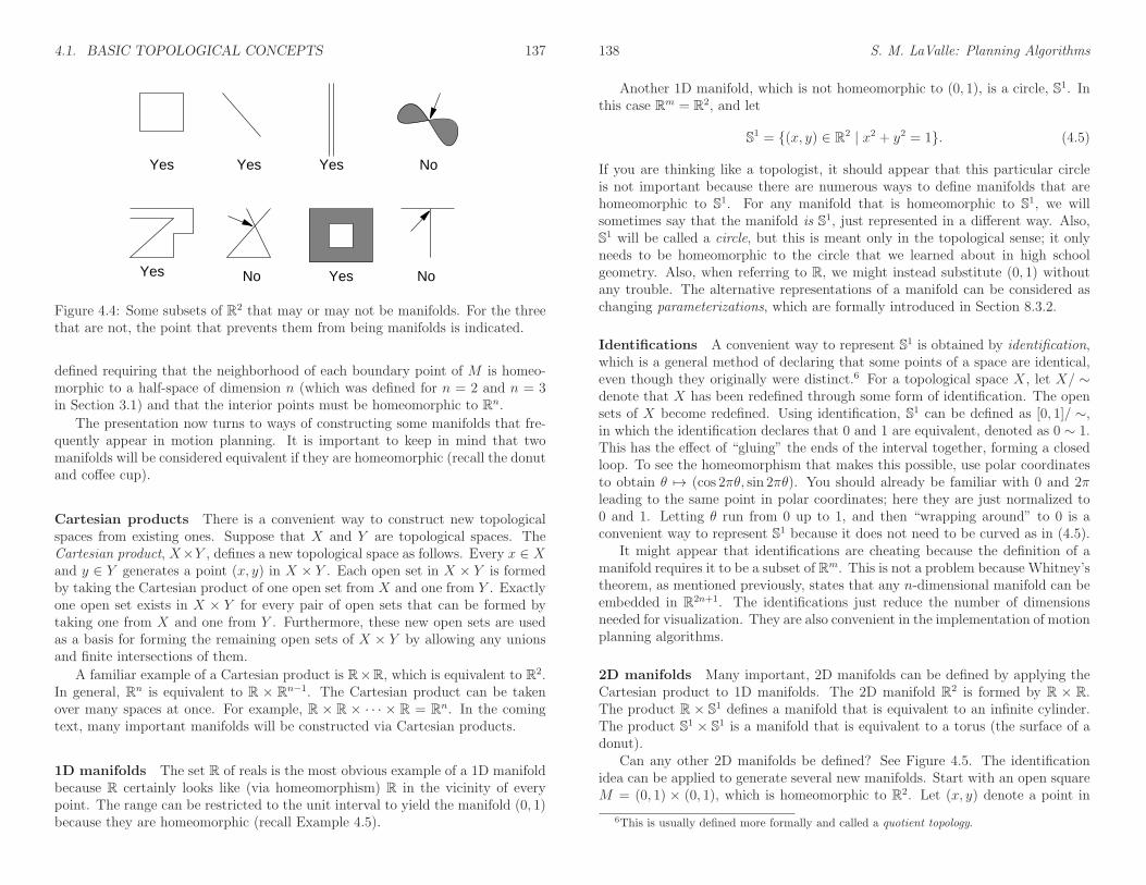
4.1. BASIC TOPOLOGICAL CONCEPTS 137
Yes
NoYes
Yes
Yes No
Yes No
Figure 4.4: Some subsets of R2 that may or may not be manifolds. For the threethat are not, the point that prevents them from being manifolds is indicated.
defined requiring that the neighborhood of each boundary point of M is homeo-morphic to a half-space of dimension n (which was defined for n = 2 and n = 3in Section 3.1) and that the interior points must be homeomorphic to Rn.
The presentation now turns to ways of constructing some manifolds that fre-quently appear in motion planning. It is important to keep in mind that twomanifolds will be considered equivalent if they are homeomorphic (recall the donutand coffee cup).
Cartesian products There is a convenient way to construct new topologicalspaces from existing ones. Suppose that X and Y are topological spaces. TheCartesian product, X×Y , defines a new topological space as follows. Every x ∈ Xand y ∈ Y generates a point (x, y) in X × Y . Each open set in X × Y is formedby taking the Cartesian product of one open set from X and one from Y . Exactlyone open set exists in X × Y for every pair of open sets that can be formed bytaking one from X and one from Y . Furthermore, these new open sets are usedas a basis for forming the remaining open sets of X × Y by allowing any unionsand finite intersections of them.
A familiar example of a Cartesian product is R×R, which is equivalent to R2.In general, Rn is equivalent to R × Rn−1. The Cartesian product can be takenover many spaces at once. For example, R × R × · · · × R = Rn. In the comingtext, many important manifolds will be constructed via Cartesian products.
1D manifolds The set R of reals is the most obvious example of a 1D manifoldbecause R certainly looks like (via homeomorphism) R in the vicinity of everypoint. The range can be restricted to the unit interval to yield the manifold (0, 1)because they are homeomorphic (recall Example 4.5).
138 S. M. LaValle: Planning Algorithms
Another 1D manifold, which is not homeomorphic to (0, 1), is a circle, S1. Inthis case Rm = R2, and let
S1 = (x, y) ∈ R2 | x2 + y2 = 1. (4.5)
If you are thinking like a topologist, it should appear that this particular circleis not important because there are numerous ways to define manifolds that arehomeomorphic to S1. For any manifold that is homeomorphic to S1, we willsometimes say that the manifold is S1, just represented in a different way. Also,S1 will be called a circle, but this is meant only in the topological sense; it onlyneeds to be homeomorphic to the circle that we learned about in high schoolgeometry. Also, when referring to R, we might instead substitute (0, 1) withoutany trouble. The alternative representations of a manifold can be considered aschanging parameterizations, which are formally introduced in Section 8.3.2.
Identifications A convenient way to represent S1 is obtained by identification,which is a general method of declaring that some points of a space are identical,even though they originally were distinct.6 For a topological space X, let X/ ∼denote that X has been redefined through some form of identification. The opensets of X become redefined. Using identification, S1 can be defined as [0, 1]/ ∼,in which the identification declares that 0 and 1 are equivalent, denoted as 0 ∼ 1.This has the effect of “gluing” the ends of the interval together, forming a closedloop. To see the homeomorphism that makes this possible, use polar coordinatesto obtain θ 7→ (cos 2πθ, sin 2πθ). You should already be familiar with 0 and 2πleading to the same point in polar coordinates; here they are just normalized to0 and 1. Letting θ run from 0 up to 1, and then “wrapping around” to 0 is aconvenient way to represent S1 because it does not need to be curved as in (4.5).
It might appear that identifications are cheating because the definition of amanifold requires it to be a subset of Rm. This is not a problem because Whitney’stheorem, as mentioned previously, states that any n-dimensional manifold can beembedded in R2n+1. The identifications just reduce the number of dimensionsneeded for visualization. They are also convenient in the implementation of motionplanning algorithms.
2D manifolds Many important, 2D manifolds can be defined by applying theCartesian product to 1D manifolds. The 2D manifold R2 is formed by R × R.The product R × S1 defines a manifold that is equivalent to an infinite cylinder.The product S1 × S1 is a manifold that is equivalent to a torus (the surface of adonut).
Can any other 2D manifolds be defined? See Figure 4.5. The identificationidea can be applied to generate several new manifolds. Start with an open squareM = (0, 1) × (0, 1), which is homeomorphic to R2. Let (x, y) denote a point in
6This is usually defined more formally and called a quotient topology.

4.1. BASIC TOPOLOGICAL CONCEPTS 139
Plane, R2 Cylinder, R× S1
Mobius band Torus, T2
Klein bottle Projective plane, RP2
Two-sphere, S2 Double torus
Figure 4.5: Some 2D manifolds that can be obtained by identifying pairs of pointsalong the boundary of a square region.
the plane. A flat cylinder is obtained by making the identification (0, y) ∼ (1, y)for all y ∈ (0, 1) and adding all of these points to M . The result is depicted inFigure 4.5 by drawing arrows where the identification occurs.
A Mobius band can be constructed by taking a strip of paper and connectingthe ends after making a 180-degree twist. This result is not homeomorphic to thecylinder. The Mobius band can also be constructed by putting the twist into theidentification, as (0, y) ∼ (1, 1 − y) for all y ∈ (0, 1). In this case, the arrows aredrawn in opposite directions. The Mobius band has the famous properties thatit has only one side (trace along the paper strip with a pencil, and you will visitboth sides of the paper) and is nonorientable (if you try to draw it in the plane,without using identification tricks, it will always have a twist).
For all of the cases so far, there has been a boundary to the set. The next fewmanifolds will not even have a boundary, even though they may be bounded. Ifyou were to live in one of them, it means that you could walk forever along anytrajectory and never encounter the edge of your universe. It might seem like ourphysical universe is unbounded, but it would only be an illusion. Furthermore,there are several distinct possibilities for the universe that are not homeomorphicto each other. In higher dimensions, such possibilities are the subject of cosmology,
140 S. M. LaValle: Planning Algorithms
which is a branch of astrophysics that uses topology to characterize the structureof our universe.
A torus can be constructed by performing identifications of the form (0, y) ∼(1, y), which was done for the cylinder, and also (x, 0) ∼ (x, 1), which identifiesthe top and bottom. Note that the point (0, 0) must be included and is identifiedwith three other points. Double arrows are used in Figure 4.5 to indicate thetop and bottom identification. All of the identification points must be added toM . Note that there are no twists. A funny interpretation of the resulting flattorus is as the universe appears for a spacecraft in some 1980s-style Asteroids-likevideo games. The spaceship flies off of the screen in one direction and appearssomewhere else, as prescribed by the identification.
Two interesting manifolds can be made by adding twists. Consider performingall of the identifications that were made for the torus, except put a twist in theside identification, as was done for the Mobius band. This yields a fascinatingmanifold called the Klein bottle, which can be embedded in R4 as a closed 2Dsurface in which the inside and the outside are the same! (This is in a sensesimilar to that of the Mobius band.) Now suppose there are twists in both thesides and the top and bottom. This results in the most bizarre manifold yet: thereal projective plane, RP2. This space is equivalent to the set of all lines in R3
that pass through the origin. The 3D version, RP3, happens to be one of the mostimportant manifolds for motion planning!
Let S2 denote the unit sphere, which is defined as
S2 = (x, y, z) ∈ R3 | x2 + y2 + z2 = 1. (4.6)
Another way to represent S2 is by making the identifications shown in the lastrow of Figure 4.5. A dashed line is indicated where the equator might appear,if we wanted to make a distorted wall map of the earth. The poles would be atthe upper left and lower right corners. The final example shown in Figure 4.5 isa double torus, which is the surface of a two-holed donut.
Higher dimensional manifolds The construction techniques used for the 2Dmanifolds generalize nicely to higher dimensions. Of course, Rn, is an n-dimensionalmanifold. An n-dimensional torus, Tn, can be made by taking a Cartesian prod-uct of n copies of S1. Note that S1 × S1 6= S2. Therefore, the notation Tn is usedfor (S1)n. Different kinds of n-dimensional cylinders can be made by forming aCartesian product Ri×Tj for positive integers i and j such that i+ j = n. Higherdimensional spheres are defined as
Sn = x ∈ Rn+1 | ‖x‖ = 1, (4.7)
in which ‖x‖ denotes the Euclidean norm of x, and n is a positive integer. Manyinteresting spaces can be made by identifying faces of the cube (0, 1)n (or even facesof a polyhedron or polytope), especially if different kinds of twists are allowed. An

4.1. BASIC TOPOLOGICAL CONCEPTS 141
n-dimensional projective space can be defined in this way, for example. Lens spacesare a family of manifolds that can be constructed by identification of polyhedralfaces [419].
Due to its coming importance in motion planning, more details are given onprojective spaces. The standard definition of an n-dimensional real projectivespace RPn is the set of all lines in Rn+1 that pass through the origin. Each lineis considered as a point in RPn. Using the definition of Sn in (4.7), note thateach of these lines in Rn+1 intersects Sn ⊂ Rn+1 in exactly two places. Theseintersection points are called antipodal, which means that they are as far fromeach other as possible on Sn. The pair is also unique for each line. If we identifyall pairs of antipodal points of Sn, a homeomorphism can be defined between eachline through the origin of Rn+1 and each antipodal pair on the sphere. This meansthat the resulting manifold, Sn/ ∼, is homeomorphic to RPn.
Another way to interpret the identification is that RPn is just the upper halfof Sn, but with every equatorial point identified with its antipodal point. Thus, ifyou try to walk into the southern hemisphere, you will find yourself on the otherside of the world walking north. It is helpful to visualize the special case of RP2
and the upper half of S2. Imagine warping the picture of RP2 from Figure 4.5from a square into a circular disc, with opposite points identified. The result stillrepresents RP2. The center of the disc can now be lifted out of the plane to formthe upper half of S2.
4.1.3 Paths and Connectivity
Central to motion planning is determining whether one part of a space is reachablefrom another. In Chapter 2, one state was reached from another by applyinga sequence of actions. For motion planning, the analog to this is connectingone point in the configuration space to another by a continuous path. Graphconnectivity is important in the discrete planning case. An analog to this fortopological spaces is presented in this section.
Paths Let X be a topological space, which for our purposes will also be amanifold. A path is a continuous function, τ : [0, 1] → X. Alternatively, R maybe used for the domain of τ . Keep in mind that a path is a function, not a setof points. Each point along the path is given by τ(s) for some s ∈ [0, 1]. Thismakes it appear as a nice generalization to the sequence of states visited when aplan from Chapter 2 is applied. Recall that there, a countable set of stages wasdefined, and the states visited could be represented as x1, x2, . . .. In the currentsetting τ(s) is used, in which s replaces the stage index. To make the connectionclearer, we could use x instead of τ to obtain x(s) for each s ∈ [0, 1].
Connected vs. path connected A topological space X is said to be connectedif it cannot be represented as the union of two disjoint, nonempty, open sets. While
142 S. M. LaValle: Planning Algorithms
this definition is rather elegant and general, if X is connected, it does not implythat a path exists between any pair of points in X thanks to crazy examples likethe topologist’s sine curve:
X = (x, y) ∈ R2 | x = 0 or y = sin(1/x). (4.8)
Consider plotting X. The sin(1/x) part creates oscillations near the y-axis inwhich the frequency tends to infinity. After union is taken with the y-axis, thisspace is connected, but there is no path that reaches the y-axis from the sinecurve.
How can we avoid such problems? The standard way to fix this is to use thepath definition directly in the definition of connectedness. A topological space Xis said to be path connected if for all x1, x2 ∈ X, there exists a path τ such thatτ(0) = x1 and τ(1) = x2. It can be shown that if X is path connected, then it isalso connected in the sense defined previously.
Another way to fix it is to make restrictions on the kinds of topological spacesthat will be considered. This approach will be taken here by assuming that alltopological spaces are manifolds. In this case, no strange things like (4.8) can hap-pen,7 and the definitions of connected and path connected coincide [232]. There-fore, we will just say a space is connected. However, it is important to rememberthat this definition of connected is sometimes inadequate, and one should reallysay that X is path connected.
Simply connected Now that the notion of connectedness has been established,the next step is to express different kinds of connectivity. This may be done byusing the notion of homotopy, which can intuitively be considered as a way tocontinuously “warp” or “morph” one path into another, as depicted in Figure4.6a.
Two paths τ1 and τ2 are called homotopic (with endpoints fixed) if there existsa continuous function h : [0, 1]× [0, 1]→ X for which the following four conditionsare met:
1. (Start with first path) h(s, 0) = τ1(s) for all s ∈ [0, 1] .
2. (End with second path) h(s, 1) = τ2(s) for all s ∈ [0, 1] .
3. (Hold starting point fixed) h(0, t) = h(0, 0) for all t ∈ [0, 1] .
4. (Hold ending point fixed) h(1, t) = h(1, 0) for all t ∈ [0, 1] .
The parameter t can be interpreted as a knob that is turned to gradually deformthe path from τ1 into τ2. The first two conditions indicate that t = 0 yields τ1
7The topologist’s sine curve is not a manifold because all open sets that contain the point(0, 0) contain some of the points from the sine curve. These open sets are not homeomorphic toR.

4.1. BASIC TOPOLOGICAL CONCEPTS 143
t = 0
t = 1
t = 1/3
t = 2/3
t = 0
t = 1
(a) (b)
Figure 4.6: (a) Homotopy continuously warps one path into another. (b) Theimage of the path cannot be continuously warped over a hole in R2 because itcauses a discontinuity. In this case, the two paths are not homotopic.
and t = 1 yields τ2, respectively. The remaining two conditions indicate that thepath endpoints are held fixed.
During the warping process, the path image cannot make a discontinuousjump. In R2, this prevents it from moving over holes, such as the one shownin Figure 4.6b. The key to preventing homotopy from jumping over some holesis that h must be continuous. In higher dimensions, however, there are manydifferent kinds of holes. For the case of R3, for example, suppose the space is likea block of Swiss cheese that contains air bubbles. Homotopy can go around the airbubbles, but it cannot pass through a hole that is drilled through the entire block ofcheese. Air bubbles and other kinds of holes that appear in higher dimensions canbe characterized by generalizing homotopy to the warping of higher dimensionalsurfaces, as opposed to paths [226].
It is straightforward to show that homotopy defines an equivalence relationon the set of all paths from some x1 ∈ X to some x2 ∈ X. The resulting notionof “equivalent paths” appears frequently in motion planning, control theory, andmany other contexts. Suppose that X is path connected. If all paths fall into thesame equivalence class, then X is called simply connected; otherwise, X is calledmultiply connected.
Groups The equivalence relation induced by homotopy starts to enter the realmof algebraic topology, which is a branch of mathematics that characterizes thestructure of topological spaces in terms of algebraic objects, such as groups. Theseresulting groups have important implications for motion planning. Therefore, wegive a brief overview. First, the notion of a group must be precisely defined. Agroup is a set, G, together with a binary operation, , such that the followinggroup axioms are satisfied:
1. (Closure) For any a, b ∈ G, the product a b ∈ G.
144 S. M. LaValle: Planning Algorithms
2. (Associativity) For all a, b, c ∈ G, (ab)c = a(bc). Hence, parenthesesare not needed, and the product may be written as a b c.
3. (Identity) There is an element e ∈ G, called the identity, such that for alla ∈ G, e a = a and a e = a.
4. (Inverse) For every element a ∈ G, there is an element a−1, called theinverse of a, for which a a−1 = e and a−1 a = e.
Here are some examples.
Example 4.7 (Simple Examples of Groups) The set of integers Z is a groupwith respect to addition. The identity is 0, and the inverse of each i is −i. The setQ\0 of rational numbers with 0 removed is a group with respect to multiplication.The identity is 1, and the inverse of every element, q, is 1/q (0 was removed toavoid division by zero).
An important property, which only some groups possess, is commutativity:a b = b a for any a, b ∈ G. The group in this case is called commutative orAbelian. We will encounter examples of both kinds of groups, both commutativeand noncommutative. An example of a commutative group is vector addition overRn. The set of all 3D rotations is an example of a noncommutative group.
The fundamental group Now an interesting group will be constructed fromthe space of paths and the equivalence relation obtained by homotopy. The funda-mental group, π1(X) (or first homotopy group), is associated with any topologicalspace, X. Let a (continuous) path for which f(0) = f(1) be called a loop. Letsome xb ∈ X be designated as a base point. For some arbitrary but fixed basepoint, xb, consider the set of all loops such that f(0) = f(1) = xb. This can bemade into a group by defining the following binary operation. Let τ1 : [0, 1]→ Xand τ2 : [0, 1] → X be two loop paths with the same base point. Their productτ = τ1 τ2 is defined as
τ(t) =
τ1(2t) if t ∈ [0, 1/2)τ2(2t− 1) if t ∈ [1/2, 1].
(4.9)
This results in a continuous loop path because τ1 terminates at xb, and τ2 beginsat xb. In a sense, the two paths are concatenated end-to-end.
Suppose now that the equivalence relation induced by homotopy is applied tothe set of all loop paths through a fixed point, xb. It will no longer be importantwhich particular path was chosen from a class; any representative may be used.The equivalence relation also applies when the set of loops is interpreted as agroup. The group operation actually occurs over the set of equivalences of paths.
Consider what happens when two paths from different equivalence classes areconcatenated using . Is the resulting path homotopic to either of the first two?

4.1. BASIC TOPOLOGICAL CONCEPTS 145
Is the resulting path homotopic if the original two are from the same homotopyclass? The answers in general are no and no, respectively. The fundamental groupdescribes how the equivalence classes of paths are related and characterizes theconnectivity of X. Since fundamental groups are based on paths, there is a niceconnection to motion planning.
Example 4.8 (A Simply Connected Space) Suppose that a topological spaceX is simply connected. In this case, all loop paths from a base point xb are ho-motopic, resulting in one equivalence class. The result is π1(X) = 1G, which isthe group that consists of only the identity element.
Example 4.9 (The Fundamental Group of S1) Suppose X = S1. In thiscase, there is an equivalence class of paths for each i ∈ Z, the set of integers.If i > 0, then it means that the path winds i times around S1 in the counter-clockwise direction and then returns to xb. If i < 0, then the path winds aroundi times in the clockwise direction. If i = 0, then the path is equivalent to onethat remains at xb. The fundamental group is Z, with respect to the operation ofaddition. If τ1 travels i1 times counterclockwise, and τ2 travels i2 times counter-clockwise, then τ = τ1 τ2 belongs to the class of loops that travel around i1 + i2times counterclockwise. Consider additive inverses. If a path travels seven timesaround S1, and it is combined with a path that travels seven times in the oppositedirection, the result is homotopic to a path that remains at xb. Thus, π1(S
1) = Z.
Example 4.10 (The Fundamental Group of Tn) For the torus, π1(Tn) = Zn,
in which the ith component of Zn corresponds to the number of times a loop pathwraps around the ith component of Tn. This makes intuitive sense because Tn isjust the Cartesian product of n circles. The fundamental group Zn is obtained bystarting with a simply connected subset of the plane and drilling out n disjoint,bounded holes. This situation arises frequently when a mobile robot must avoidcollision with n disjoint obstacles in the plane.
By now it seems that the fundamental group simply keeps track of how manytimes a path travels around holes. This next example yields some very bizarrebehavior that helps to illustrate some of the interesting structure that arises inalgebraic topology.
Example 4.11 (The Fundamental Group of RP2) Suppose X = RP2, theprojective plane. In this case, there are only two equivalence classes on the space ofloop paths. All paths that “wrap around” an even number of times are homotopic.Likewise, all paths that wrap around an odd number of times are homotopic. Thisstrange behavior is illustrated in Figure 4.7. The resulting fundamental group
146 S. M. LaValle: Planning Algorithms
1
11
1
2
2
1
12
2
(a) (b) (c)
Figure 4.7: An illustration of why π1(RP2) = Z2. The integers 1 and 2 indicate
precisely where a path continues when it reaches the boundary. (a) Two paths areshown that are not equivalent. (b) A path that winds around twice is shown. (c)This is homotopic to a loop path that does not wind around at all. Eventually,the part of the path that appears at the bottom is pulled through the top. Itfinally shrinks into an arbitrarily small loop.
therefore has only two elements: π1(RP2) = Z2, the cyclic group of order 2, which
corresponds to addition mod 2. This makes intuitive sense because the groupkeeps track of whether a sum of integers is odd or even, which in this applicationcorresponds to the total number of traversals over the square representation ofRP2. The fundamental group is the same for RP3, which arises in Section 4.2.2because it is homeomorphic to the set of 3D rotations. Thus, there are surprisinglyonly two path classes for the set of 3D rotations.
Unfortunately, two topological spaces may have the same fundamental groupeven if the spaces are not homeomorphic. For example, Z is the fundamentalgroup of S1, the cylinder, R × S1, and the Mobius band. In the last case, thefundamental group does not indicate that there is a “twist” in the space. Anotherproblem is that spaces with interesting connectivity may be declared as simplyconnected. The fundamental group of the sphere S2 is just 1G, the same as forR2. Try envisioning loop paths on the sphere; it can be seen that they all fall intoone equivalence class. Hence, S2 is simply connected. The fundamental group alsoneglects bubbles in R3 because the homotopy can warp paths around them. Someof these troubles can be fixed by defining second-order homotopy groups. Forexample, a continuous function, [0, 1] × [0, 1] → X, of two variables can be usedinstead of a path. The resulting homotopy generates a kind of sheet or surfacethat can be warped through the space, to yield a homotopy group π2(X) thatwraps around bubbles in R3. This idea can be extended beyond two dimensionsto detect many different kinds of holes in higher dimensional spaces. This leads tothe higher order homotopy groups. A stronger concept than simply connected for
4.2. DEFINING THE CONFIGURATION SPACE 147
a space is that its homotopy groups of all orders are equal to the identity group.This prevents all kinds of holes from occurring and implies that a space, X, iscontractible, which means a kind of homotopy can be constructed that shrinks Xto a point [226]. In the plane, the notions of contractible and simply connected areequivalent; however, in higher dimensional spaces, such as those arising in motionplanning, the term contractible should be used to indicate that the space has nointerior obstacles (holes).
An alternative to basing groups on homotopy is to derive them using homology,which is based on the structure of cell complexes instead of homotopy mappings.This subject is much more complicated to present, but it is more powerful forproving theorems in topology. See the literature overview at the end of the chapterfor suggested further reading on algebraic topology.
4.2 Defining the Configuration Space
This section defines the manifolds that arise from the transformations of Chapter3. If the robot has n degrees of freedom, the set of transformations is usually amanifold of dimension n. This manifold is called the configuration space of therobot, and its name is often shortened to C-space. In this book, the C-spacemay be considered as a special state space. To solve a motion planning problem,algorithms must conduct a search in the C-space. The C-space provides a powerfulabstraction that converts the complicated models and transformations of Chapter3 into the general problem of computing a path that traverses a manifold. Bydeveloping algorithms directly for this purpose, they apply to a wide variety ofdifferent kinds of robots and transformations. In Section 4.3 the problem will becomplicated by bringing obstacles into the configuration space, but in Section 4.2there will be no obstacles.
4.2.1 2D Rigid Bodies: SE(2)
Section 3.2.2 expressed how to transform a rigid body in R2 by a homogeneoustransformation matrix, T , given by (3.35). The task in this chapter is to char-acterize the set of all possible rigid-body transformations. Which manifold willthis be? Here is the answer and brief explanation. Since any xt, yt ∈ R can beselected for translation, this alone yields a manifoldM1 = R2. Independently, anyrotation, θ ∈ [0, 2π), can be applied. Since 2π yields the same rotation as 0, theycan be identified, which makes the set of 2D rotations into a manifold, M2 = S1.To obtain the manifold that corresponds to all rigid-body motions, simply takeC =M1×M2 = R2×S1. The answer to the question is that the C-space is a kindof cylinder.
Now we give a more detailed technical argument. The main purpose is thatsuch a simple, intuitive argument will not work for the 3D case. Our approach is
148 S. M. LaValle: Planning Algorithms
to introduce some of the technical machinery here for the 2D case, which is easierto understand, and then extend it to the 3D case in Section 4.2.2.
Matrix groups The first step is to consider the set of transformations as agroup, in addition to a topological space.8 We now derive several important groupsfrom sets of matrices, ultimately leading to SO(n), the group of n × n rotationmatrices, which is very important for motion planning. The set of all nonsingularn × n real-valued matrices is called the general linear group, denoted by GL(n),with respect to matrix multiplication. Each matrix A ∈ GL(n) has an inverseA−1 ∈ GL(n), which when multiplied yields the identity matrix, AA−1 = I. Thematrices must be nonsingular for the same reason that 0 was removed from Q. Theanalog of division by zero for matrix algebra is the inability to invert a singularmatrix.
Many interesting groups can be formed from one group, G1, by removing someelements to obtain a subgroup, G2. To be a subgroup, G2 must be a subset of G1
and satisfy the group axioms. We will arrive at the set of rotation matricesby constructing subgroups. One important subgroup of GL(n) is the orthogonalgroup, O(n), which is the set of all matrices A ∈ GL(n) for which AAT = I,in which AT denotes the matrix transpose of A. These matrices have orthogonalcolumns (the inner product of any pair is zero) and the determinant is always 1or −1. Thus, note that AAT takes the inner product of every pair of columns. Ifthe columns are different, the result must be 0; if they are the same, the resultis 1 because AAT = I. The special orthogonal group, SO(n), is the subgroup ofO(n) in which every matrix has determinant 1. Another name for SO(n) is thegroup of n-dimensional rotation matrices.
A chain of groups, SO(n) ≤ O(n) ≤ GL(n), has been described in which≤ denotes “a subgroup of.” Each group can also be considered as a topologicalspace. The set of all n×n matrices (which is not a group with respect to multipli-cation) with real-valued entries is homeomorphic to Rn2
because n2 entries in thematrix can be independently chosen. For GL(n), singular matrices are removed,but an n2-dimensional manifold is nevertheless obtained. For O(n), the expres-sion AAT = I corresponds to n2 algebraic equations that have to be satisfied.This should substantially drop the dimension. Note, however, that many of theequations are redundant (pick your favorite value for n, multiply the matrices,and see what happens). There are only (n2 ) ways (pairwise combinations) to takethe inner product of pairs of columns, and there are n equations that require themagnitude of each column to be 1. This yields a total of n(n+ 1)/2 independentequations. Each independent equation drops the manifold dimension by one, and
8The groups considered in this section are actually Lie groups because they are smoothmanifolds [45]. We will not use that name here, however, because the notion of a smoothstructure has not yet been defined. Readers familiar with Lie groups, however, will recognizemost of the coming concepts. Some details on Lie groups appear later in Sections 15.4.3 and15.5.1.

4.2. DEFINING THE CONFIGURATION SPACE 149
the resulting dimension of O(n) is n2 − n(n + 1)/2 = n(n− 1)/2, which is easilyremembered as (n2 ). To obtain SO(n), the constraint detA = 1 is added, whicheliminates exactly half of the elements of O(n) but keeps the dimension the same.
Example 4.12 (Matrix Subgroups) It is helpful to illustrate the concepts forn = 2. The set of all 2× 2 matrices is
(
a bc d
) ∣
∣
∣
∣
a, b, c, d ∈ R
, (4.10)
which is homeomorphic to R4. The group GL(2) is formed from the set of allnonsingular 2×2 matrices, which introduces the constraint that ad− bc 6= 0. Theset of singular matrices forms a 3D manifold with boundary in R4, but all otherelements of R4 are in GL(2); therefore, GL(2) is a 4D manifold.
Next, the constraint AAT = I is enforced to obtain O(2). This becomes
(
a bc d
)(
a cb d
)
=
(
1 00 1
)
, (4.11)
which directly yields four algebraic equations:
a2 + b2 = 1 (4.12)
ac+ bd = 0 (4.13)
ca+ db = 0 (4.14)
c2 + d2 = 1. (4.15)
Note that (4.14) is redundant. There are two kinds of equations. One equation,given by (4.13), forces the inner product of the columns to be 0. There is onlyone because (n2 ) = 1 for n = 2. Two other constraints, (4.12) and (4.15), force therows to be unit vectors. There are two because n = 2. The resulting dimension ofthe manifold is (n2 ) = 1 because we started with R4 and lost three dimensions from(4.12), (4.13), and (4.15). What does this manifold look like? Imagine that thereare two different two-dimensional unit vectors, (a, b) and (c, d). Any value can bechosen for (a, b) as long as a2 + b2 = 1. This looks like S1, but the inner productof (a, b) and (c, d) must also be 0. Therefore, for each value of (a, b), there aretwo choices for c and d: 1) c = b and d = −a, or 2) c = −b and d = a. It appearsthat there are two circles! The manifold is S1 ⊔ S1, in which ⊔ denotes the unionof disjoint sets. Note that this manifold is not connected because no path existsfrom one circle to the other.
The final step is to require that detA = ad− bc = 1, to obtain SO(2), the setof all 2D rotation matrices. Without this condition, there would be matrices thatproduce a rotated mirror image of the rigid body. The constraint simply forcesthe choice for c and d to be c = −b and a = d. This throws away one of the circlesfrom O(2), to obtain a single circle for SO(2). We have finally obtained what youalready knew: SO(2) is homeomorphic to S1. The circle can be parameterized
150 S. M. LaValle: Planning Algorithms
using polar coordinates to obtain the standard 2D rotation matrix, (3.31), givenin Section 3.2.2.
Special Euclidean group Now that the group of rotations, SO(n), is charac-terized, the next step is to allow both rotations and translations. This correspondsto the set of all (n+ 1)× (n+ 1) transformation matrices of the form
(
R v0 1
) ∣
∣
∣
∣
R ∈ SO(n) and v ∈ Rn
. (4.16)
This should look like a generalization of (3.52) and (3.56), which were for n = 2and n = 3, respectively. The R part of the matrix achieves rotation of an n-dimensional body in Rn, and the v part achieves translation of the same body.The result is a group, SE(n), which is called the special Euclidean group. As atopological space, SE(n) is homeomorphic to Rn × SO(n), because the rotationmatrix and translation vectors may be chosen independently. In the case of n = 2,this means SE(2) is homeomorphic to R2 × S1, which verifies what was statedat the beginning of this section. Thus, the C-space of a 2D rigid body that cantranslate and rotate in the plane is
C = R2 × S1. (4.17)
To be more precise, ∼= should be used in the place of = to indicate that C couldbe any space homeomorphic to R2 × S1; however, this notation will mostly beavoided.
Interpreting the C-space It is important to consider the topological impli-cations of C. Since S1 is multiply connected, R × S1 and R2 × S1 are multiplyconnected. It is difficult to visualize C because it is a 3D manifold; however,there is a nice interpretation using identification. Start with the open unit cube,(0, 1)3 ⊂ R3. Include the boundary points of the form (x, y, 0) and (x, y, 1), andmake the identification (x, y, 0) ∼ (x, y, 1) for all x, y ∈ (0, 1). This means thatwhen traveling in the x and y directions, there is a “frontier” to the C-space;however, traveling in the z direction causes a wraparound.
It is very important for a motion planning algorithm to understand that thiswraparound exists. For example, consider R× S1 because it is easier to visualize.Imagine a path planning problem for which C = R×S1, as depicted in Figure 4.8.Suppose the top and bottom are identified to make a cylinder, and there is anobstacle across the middle. Suppose the task is to find a path from qI to qG. Ifthe top and bottom were not identified, then it would not be possible to connectqI to qG; however, if the algorithm realizes it was given a cylinder, the task isstraightforward. In general, it is very important to understand the topology of C;otherwise, potential solutions will be lost.
The next section addresses SE(n) for n = 3. The main difficulty is determiningthe topology of SO(3). At least we do not have to consider n > 3 in this book.

4.2. DEFINING THE CONFIGURATION SPACE 151
qI
qG
Figure 4.8: A planning algorithm may have to cross the identification boundaryto find a solution path.
4.2.2 3D Rigid Bodies: SE(3)
One might expect that defining C for a 3D rigid body is an obvious extension of the2D case; however, 3D rotations are significantly more complicated. The resultingC-space will be a six-dimensional manifold, C = R3 × RP3. Three dimensionscome from translation and three more come from rotation.
The main quest in this section is to determine the topology of SO(3). InSection 3.2.3, yaw, pitch, and roll were used to generate rotation matrices. Theseangles are convenient for visualization, performing transformations in software,and also for deriving the DH parameters. However, these were concerned withapplying a single rotation, whereas the current problem is to characterize the setof all rotations. It is possible to use α, β, and γ to parameterize the set of rotations,but it causes serious troubles. There are some cases in which nonzero angles yieldthe identity rotation matrix, which is equivalent to α = β = γ = 0. There arealso cases in which a continuum of values for yaw, pitch, and roll angles yield thesame rotation matrix. These problems destroy the topology, which causes boththeoretical and practical difficulties in motion planning.
Consider applying the matrix group concepts from Section 4.2.1. The generallinear group GL(3) is homeomorphic to R9. The orthogonal group, O(3), is de-termined by imposing the constraint AAT = I. There are (32) = 3 independentequations that require distinct columns to be orthogonal, and three independentequations that force the magnitude of each column to be 1. This means that O(3)has three dimensions, which matches our intuition since there were three rotationparameters in Section 3.2.3. To obtain SO(3), the last constraint, detA = 1,is added. Recall from Example 4.12 that SO(2) consists of two circles, and theconstraint detA = 1 selects one of them. In the case of O(3), there are twothree-spheres, S3 ⊔ S3, and detA = 1 selects one of them. However, there is oneadditional complication: Antipodal points on these spheres generate the same ro-tation matrix. This will be seen shortly when quaternions are used to parameterizeSO(3).
152 S. M. LaValle: Planning Algorithms
Using complex numbers to represent SO(2) Before introducing quater-nions to parameterize 3D rotations, consider using complex numbers to param-eterize 2D rotations. Let the term unit complex number refer to any complexnumber, a+ bi, for which a2 + b2 = 1.
The set of all unit complex numbers forms a group under multiplication. It willbe seen that it is “the same” group as SO(2). This idea needs to be made moreprecise. Two groups, G and H, are considered “the same” if they are isomorphic,which means that there exists a bijective function f : G → H such that for alla, b ∈ G, f(a)f(b) = f(ab). This means that we can perform some calculationsin G, map the result to H, perform more calculations, and map back to G withoutany trouble. The sets G and H are just two alternative ways to express the samegroup.
The unit complex numbers and SO(2) are isomorphic. To see this clearly,recall that complex numbers can be represented in polar form as reiθ; a unitcomplex number is simply eiθ. A bijective mapping can be made between 2Drotation matrices and unit complex numbers by letting eiθ correspond to therotation matrix (3.31).
If complex numbers are used to represent rotations, it is important that theybehave algebraically in the same way. If two rotations are combined, the matricesare multiplied. The equivalent operation is multiplication of complex numbers.Suppose that a 2D robot is rotated by θ1, followed by θ2. In polar form, the com-plex numbers are multiplied to yield eiθ1eiθ2 = ei(θ1+θ2), which clearly represents arotation of θ1 + θ2. If the unit complex number is represented in Cartesian form,then the rotations corresponding to a1 + b1i and a2 + b2i are combined to obtain(a1a2−b1b2)+(a1b2+a2b1)i. Note that here we have not used complex numbers toexpress the solution to a polynomial equation, which is their more popular use; wesimply borrowed their nice algebraic properties. At any time, a complex numbera+ bi can be converted into the equivalent rotation matrix
R(a, b) =
(
a −bb a
)
. (4.18)
Recall that only one independent parameter needs to be specified because a2 +b2 = 1. Hence, it appears that the set of unit complex numbers is the samemanifold as SO(2), which is the circle S1 (recall, that “same” means in the senseof homeomorphism).
Quaternions The manner in which complex numbers were used to represent2D rotations will now be adapted to using quaternions to represent 3D rotations.Let H represent the set of quaternions, in which each quaternion, h ∈ H, isrepresented as h = a + bi + cj + dk, and a, b, c, d ∈ R. A quaternion can beconsidered as a four-dimensional vector. The symbols i, j, and k are used to denotethree “imaginary” components of the quaternion. The following relationships aredefined: i2 = j2 = k2 = ijk = −1, from which it follows that ij = k, jk = i, and
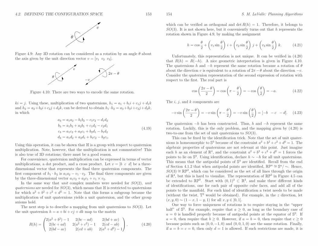
4.2. DEFINING THE CONFIGURATION SPACE 153
v
θ
Figure 4.9: Any 3D rotation can be considered as a rotation by an angle θ aboutthe axis given by the unit direction vector v = [v1 v2 v3].
v
θ2π − θ
−v
Figure 4.10: There are two ways to encode the same rotation.
ki = j. Using these, multiplication of two quaternions, h1 = a1 + b1i + c1j + d1kand h2 = a2+b2i+c2j+d2k, can be derived to obtain h1 ·h2 = a3+b3i+c3j+d3k,in which
a3 = a1a2 − b1b2 − c1c2 − d1d2b3 = a1b2 + a2b1 + c1d2 − c2d1c3 = a1c2 + a2c1 + b2d1 − b1d2d3 = a1d2 + a2d1 + b1c2 − b2c1.
(4.19)
Using this operation, it can be shown that H is a group with respect to quaternionmultiplication. Note, however, that the multiplication is not commutative! Thisis also true of 3D rotations; there must be a good reason.
For convenience, quaternion multiplication can be expressed in terms of vectormultiplications, a dot product, and a cross product. Let v = [b c d] be a three-dimensional vector that represents the final three quaternion components. Thefirst component of h1 · h2 is a1a2 − v1 · v2. The final three components are givenby the three-dimensional vector a1v2 + a2v1 + v1 × v2.
In the same way that unit complex numbers were needed for SO(2), unitquaternions are needed for SO(3), which means that H is restricted to quaternionsfor which a2 + b2 + c2 + d2 = 1. Note that this forms a subgroup because themultiplication of unit quaternions yields a unit quaternion, and the other groupaxioms hold.
The next step is to describe a mapping from unit quaternions to SO(3). Letthe unit quaternion h = a+ bi+ cj + dk map to the matrix
R(h) =
2(a2 + b2)− 1 2(bc− ad) 2(bd+ ac)2(bc+ ad) 2(a2 + c2)− 1 2(cd− ab)2(bd− ac) 2(cd+ ab) 2(a2 + d2)− 1
, (4.20)
154 S. M. LaValle: Planning Algorithms
which can be verified as orthogonal and detR(h) = 1. Therefore, it belongs toSO(3). It is not shown here, but it conveniently turns out that h represents therotation shown in Figure 4.9, by making the assignment
h = cosθ
2+
(
v1 sinθ
2
)
i+
(
v2 sinθ
2
)
j +
(
v3 sinθ
2
)
k. (4.21)
Unfortunately, this representation is not unique. It can be verified in (4.20)that R(h) = R(−h). A nice geometric interpretation is given in Figure 4.10.The quaternions h and −h represent the same rotation because a rotation of θabout the direction v is equivalent to a rotation of 2π− θ about the direction −v.Consider the quaternion representation of the second expression of rotation withrespect to the first. The real part is
cos
(
2π − θ2
)
= cos
(
π − θ
2
)
= − cos
(
θ
2
)
= −a. (4.22)
The i, j, and k components are
−v sin(
2π − θ2
)
= −v sin(
π − θ
2
)
= −v sin(
θ
2
)
= [−b − c − d]. (4.23)
The quaternion −h has been constructed. Thus, h and −h represent the samerotation. Luckily, this is the only problem, and the mapping given by (4.20) istwo-to-one from the set of unit quaternions to SO(3).
This can be fixed by the identification trick. Note that the set of unit quater-nions is homeomorphic to S3 because of the constraint a2 + b2 + c2 + d2 = 1. Thealgebraic properties of quaternions are not relevant at this point. Just imagineeach h as an element of R4, and the constraint a2 + b2 + c2 + d2 = 1 forces thepoints to lie on S3. Using identification, declare h ∼ −h for all unit quaternions.This means that the antipodal points of S3 are identified. Recall from the endof Section 4.1.2 that when antipodal points are identified, RPn ∼= Sn/ ∼. Hence,SO(3) ∼= RP3, which can be considered as the set of all lines through the originof R4, but this is hard to visualize. The representation of RP2 in Figure 4.5 canbe extended to RP3. Start with (0, 1)3 ⊂ R3, and make three different kindsof identifications, one for each pair of opposite cube faces, and add all of thepoints to the manifold. For each kind of identification a twist needs to be made(without the twist, T3 would be obtained). For example, in the z direction, let(x, y, 0) ∼ (1− x, 1− y, 1) for all x, y ∈ [0, 1].
One way to force uniqueness of rotations is to require staying in the “upperhalf” of S3. For example, require that a ≥ 0, as long as the boundary case ofa = 0 is handled properly because of antipodal points at the equator of S3. Ifa = 0, then require that b ≥ 0. However, if a = b = 0, then require that c ≥ 0because points such as (0, 0,−1, 0) and (0, 0, 1, 0) are the same rotation. Finally,if a = b = c = 0, then only d = 1 is allowed. If such restrictions are made, it is

4.2. DEFINING THE CONFIGURATION SPACE 155
important, however, to remember the connectivity of RP3. If a path travels acrossthe equator of S3, it must be mapped to the appropriate place in the “northernhemisphere.” At the instant it hits the equator, it must move to the antipodalpoint. These concepts are much easier to visualize if you remove a dimension andimagine them for S2 ⊂ R3, as described at the end of Section 4.1.2.
Using quaternion multiplication The representation of rotations boiled downto picking points on S3 and respecting the fact that antipodal points give the sameelement of SO(3). In a sense, this has nothing to do with the algebraic propertiesof quaternions. It merely means that SO(3) can be parameterized by pickingpoints in S3, just like SO(2) was parameterized by picking points in S1 (ignoringthe antipodal identification problem for SO(3)).
However, one important reason why the quaternion arithmetic was introducedis that the group of unit quaternions with h and −h identified is also isomorphic toSO(3). This means that a sequence of rotations can be multiplied together usingquaternion multiplication instead of matrix multiplication. This is importantbecause fewer operations are required for quaternion multiplication in comparisonto matrix multiplication. At any point, (4.20) can be used to convert the resultback into a matrix; however, this is not even necessary. It turns out that apoint in the world, (x, y, z) ∈ R3, can be transformed by directly using quaternionarithmetic. An analog to the complex conjugate from complex numbers is needed.For any h = a+ bi+ cj + dk ∈ H, let h∗ = a− bi− cj − dk be its conjugate. Forany point (x, y, z) ∈ R3, let p ∈ H be the quaternion 0 + xi + yj + zk. It can beshown (with a lot of algebra) that the rotated point (x, y, z) is given by h · p · h∗.The i, j, k components of the resulting quaternion are new coordinates for thetransformed point. It is equivalent to having transformed (x, y, z) with the matrixR(h).
Finding quaternion parameters from a rotation matrix Recall from Sec-tion 3.2.3 that given a rotation matrix (3.43), the yaw, pitch, and roll parameterscould be directly determined using the atan2 function. It turns out that thequaternion representation can also be determined directly from the matrix. Thisis the inverse of the function in (4.20).9
For a given rotation matrix (3.43), the quaternion parameters h = a + bi +cj + dk can be computed as follows [113]. The first component is
a = 12
√r11 + r22 + r33 + 1, (4.24)
and if a 6= 0, then
b =r32 − r23
4a, (4.25)
9Since that function was two-to-one, it is technically not an inverse until the quaternions arerestricted to the upper hemisphere, as described previously.
156 S. M. LaValle: Planning Algorithms
c =r13 − r31
4a, (4.26)
and
d =r21 − r12
4a. (4.27)
If a = 0, then the previously mentioned equator problem occurs. In this case,
b =r13r12
√
r212r213 + r212r
223 + r213r
223
, (4.28)
c =r12r23
√
r212r213 + r212r
223 + r213r
223
, (4.29)
andd =
r13r23√
r212r213 + r212r
223 + r213r
223
. (4.30)
This method fails if r12 = r23 = 0 or r13 = r23 = 0 or r12 = r23 = 0. Thesecorrespond precisely to the cases in which the rotation matrix is a yaw, (3.39),pitch, (3.40), or roll, (3.41), which can be detected in advance.
Special Euclidean group Now that the complicated part of representing SO(3)has been handled, the representation of SE(3) is straightforward. The generalform of a matrix in SE(3) is given by (4.16), in which R ∈ SO(3) and v ∈ R3.Since SO(3) ∼= RP3, and translations can be chosen independently, the resultingC-space for a rigid body that rotates and translates in R3 is
C = R3 × RP3, (4.31)
which is a six-dimensional manifold. As expected, the dimension of C is exactlythe number of degrees of freedom of a free-floating body in space.
4.2.3 Chains and Trees of Bodies
If there are multiple bodies that are allowed to move independently, then theirC-spaces can be combined using Cartesian products. Let Ci denote the C-spaceof Ai. If there are n free-floating bodies in W = R2 or W = R3, then
C = C1 × C2 × · · · × Cn. (4.32)
If the bodies are attached to form a kinematic chain or kinematic tree, theneach C-space must be considered on a case-by-case basis. There is no general rulethat simplifies the process. One thing to generally be careful about is that the fullrange of motion might not be possible for typical joints. For example, a revolutejoint might not be able to swing all of the way around to enable any θ ∈ [0, 2π).If θ cannot wind around S1, then the C-space for this joint is homeomorphic to R
instead of S1. A similar situation occurs for a spherical joint. A typical ball joint
4.3. CONFIGURATION SPACE OBSTACLES 157
cannot achieve any orientation in SO(3) due to mechanical obstructions. In thiscase, the C-space is not RP3 because part of SO(3) is missing.
Another complication is that the DH parameterization of Section 3.3.2 is de-signed to facilitate the assignment of coordinate frames and computation of trans-formations, but it neglects considerations of topology. For example, a commonapproach to representing a spherical robot wrist is to make three zero-length linksthat each behave as a revolute joint. If the range of motion is limited, this mightnot cause problems, but in general the problems would be similar to using yaw,pitch, and roll to represent SO(3). There may be multiple ways to express thesame arm configuration.
Several examples are given below to help in determining C-spaces for chainsand trees of bodies. Suppose W = R2, and there is a chain of n bodies that areattached by revolute joints. Suppose that the first joint is capable of rotation onlyabout a fixed point (e.g., it spins around a nail). If each joint has the full rangeof motion θi ∈ [0, 2π), the C-space is
C = S1 × S1 × · · · × S1 = Tn. (4.33)
However, if each joint is restricted to θi ∈ (−π/2, π/2), then C = Rn. If anytransformation in SE(2) can be applied to A1, then an additional R2 is needed.In the case of restricted joint motions, this yields Rn+2. If the joints can achieveany orientation, then C = R2 × Tn. If there are prismatic joints, then each jointcontributes R to the C-space.
Recall from Figure 3.12 that for W = R3 there are six different kinds ofjoints. The cases of revolute and prismatic joints behave the same as forW = R2.Each screw joint contributes R. A cylindrical joint contributes R× S1, unless itsrotational motion is restricted. A planar joint contributes R2 × S1 because anytransformation in SE(2) is possible. If its rotational motions are restricted, thenit contributes R3. Finally, a spherical joint can theoretically contribute RP3. Inpractice, however, this rarely occurs. It is more likely to contribute R2× S1 or R3
after restrictions are imposed. Note that if the first joint is a free-floating body,then it contributes R3 × RP3.
Kinematic trees can be handled in the same way as kinematic chains. Oneissue that has not been mentioned is that there might be collisions between thelinks. This has been ignored up to this point, but obviously this imposes verycomplicated restrictions. The concepts from Section 4.3 can be applied to handlethis case and the placement of additional obstacles in W . Reasoning about thesekinds of restrictions and the path connectivity of the resulting space is indeed themain point of motion planning.
4.3 Configuration Space Obstacles
Section 4.2 defined C, the manifold of robot transformations in the absence ofany collision constraints. The current section removes from C the configurations
158 S. M. LaValle: Planning Algorithms
that either cause the robot to collide with obstacles or cause some specified linksof the robot to collide with each other. The removed part of C is referred to asthe obstacle region. The leftover space is precisely what a solution path musttraverse. A motion planning algorithm must find a path in the leftover spacefrom an initial configuration to a goal configuration. Finally, after the models ofChapter 3 and the previous sections of this chapter, the motion planning problemcan be precisely described.
4.3.1 Definition of the Basic Motion Planning Problem
Obstacle region for a rigid body Suppose that the world, W = R2 or W =R3, contains an obstacle region, O ⊂ W . Assume here that a rigid robot, A ⊂ W ,is defined; the case of multiple links will be handled shortly. Assume that bothA and O are expressed as semi-algebraic models (which includes polygonal andpolyhedral models) from Section 3.1. Let q ∈ C denote the configuration of A, inwhich q = (xt, yt, θ) for W = R2 and q = (xt, yt, zt, h) for W = R3 (h representsthe unit quaternion).
The obstacle region, Cobs ⊆ C, is defined as
Cobs = q ∈ C | A(q) ∩ O 6= ∅, (4.34)
which is the set of all configurations, q, at which A(q), the transformed robot,intersects the obstacle region, O. Since O and A(q) are closed sets in W , theobstacle region is a closed set in C.
The leftover configurations are called the free space, which is defined and de-noted as Cfree = C \ Cobs. Since C is a topological space and Cobs is closed, Cfreemust be an open set. This implies that the robot can come arbitrarily close tothe obstacles while remaining in Cfree. If A “touches” O,
int(O) ∩ int(A(q)) = ∅ and O ∩A(q) 6= ∅, (4.35)
then q ∈ Cobs (recall that int means the interior). The condition above indicatesthat only their boundaries intersect.
The idea of getting arbitrarily close may be nonsense in practical robotics, butit makes a clean formulation of the motion planning problem. Since Cfree is open,it becomes impossible to formulate some optimization problems, such as findingthe shortest path. In this case, the closure, cl(Cfree), should instead be used, asdescribed in Section 7.7.
Obstacle region for multiple bodies If the robot consists of multiple bodies,the situation is more complicated. The definition in (4.34) only implies that therobot does not collide with the obstacles; however, if the robot consists of multiplebodies, then it might also be appropriate to avoid collisions between different linksof the robot. Let the robot be modeled as a collection, A1,A2, . . . ,Am, of m

4.3. CONFIGURATION SPACE OBSTACLES 159
links, which may or may not be attached together by joints. A single configurationvector q is given for the entire collection of links. We will write Ai(q) for eachlink, i, even though some of the parameters of q may be irrelevant for moving linkAi. For example, in a kinematic chain, the configuration of the second body doesnot depend on the angle between the ninth and tenth bodies.
Let P denote the set of collision pairs, in which each collision pair, (i, j) ∈ P ,represents a pair of link indices i, j ∈ 1, 2, . . . ,m, such that i 6= j. If (i, j)appears in P , it means that Ai and Aj are not allowed to be in a configuration,q, for which Ai(q) ∩ Aj(q) 6= ∅. Usually, P does not represent all pairs becauseconsecutive links are in contact all of the time due to the joint that connects them.One common definition for P is that each link must avoid collisions with any linksto which it is not attached by a joint. For m bodies, P is generally of size O(m2);however, in practice it is often possible to eliminate many pairs by some geometricanalysis of the linkage. Collisions between some pairs of links may be impossibleover all of C, in which case they do not need to appear in P .
Using P , the consideration of robot self-collisions is added to the definition ofCobs to obtain
Cobs =(
m⋃
i=1
q ∈ C | Ai(q) ∩ O 6= ∅)
⋃
(
⋃
[i,j]∈P
q ∈ C | Ai(q) ∩ Aj(q) 6= ∅)
.
(4.36)Thus, a configuration q ∈ C is in Cobs if at least one link collides with O or a pairof links indicated by P collide with each other.
Definition of basic motion planning Finally, enough tools have been intro-duced to precisely define the motion planning problem. The problem is concep-tually illustrated in Figure 4.11. The main difficulty is that it is neither straight-forward nor efficient to construct an explicit boundary or solid representation ofeither Cfree or Cobs. The components are as follows:
Formulation 4.1 (The Piano Mover’s Problem)
1. A world W in which either W = R2 or W = R3.
2. A semi-algebraic obstacle region O ⊂ W in the world.
3. A semi-algebraic robot is defined in W . It may be a rigid robot A or acollection of m links, A1,A2, . . . ,Am.
4. The configuration space C determined by specifying the set of all possibletransformations that may be applied to the robot. From this, Cobs and Cfreeare derived.
5. A configuration, qI ∈ Cfree designated as the initial configuration.
160 S. M. LaValle: Planning Algorithms
Cobs
qI
qG
Cfree
Cobs
Cobs
Figure 4.11: The basic motion planning problem is conceptually very simple usingC-space ideas. The task is to find a path from qI to qG in Cfree. The entire blobrepresents C = Cfree ∪ Cobs.
6. A configuration qG ∈ Cfree designated as the goal configuration. The initialand goal configurations together are often called a query pair (or query) anddesignated as (qI , qG).
7. A complete algorithm must compute a (continuous) path, τ : [0, 1]→ Cfree,such that τ(0) = qI and τ(1) = qG, or correctly report that such a path doesnot exist.
It was shown by Reif [409] that this problem is PSPACE-hard, which impliesNP-hard. The main problem is that the dimension of C is unbounded.
4.3.2 Explicitly Modeling Cobs: The Translational Case
It is important to understand how to construct a representation of Cobs. In somealgorithms, especially the combinatorial methods of Chapter 6, this representsan important first step to solving the problem. In other algorithms, especiallythe sampling-based planning algorithms of Chapter 5, it helps to understand whysuch constructions are avoided due to their complexity.
The simplest case for characterizing Cobs is when C = Rn for n = 1, 2, and3, and the robot is a rigid body that is restricted to translation only. Underthese conditions, Cobs can be expressed as a type of convolution. For any two setsX, Y ⊂ Rn, let their Minkowski difference10 be defined as
X ⊖ Y = x− y ∈ Rn | x ∈ X and y ∈ Y , (4.37)
10In some contexts, which include mathematics and image processing, the Minkowski differ-
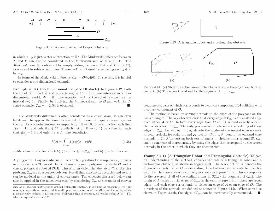
4.3. CONFIGURATION SPACE OBSTACLES 161
-4 -3 -2 -1
A
O
Cobs
−A
6543210
Figure 4.12: A one-dimensional C-space obstacle.
in which x−y is just vector subtraction on Rn. The Minkowski difference betweenX and Y can also be considered as the Minkowski sum of X and −Y . TheMinkowski sum ⊕ is obtained by simply adding elements of X and Y in (4.37),as opposed to subtracting them. The set −Y is obtained by replacing each y ∈ Yby −y.
In terms of the Minkowski difference, Cobs = O⊖A(0). To see this, it is helpfulto consider a one-dimensional example.
Example 4.13 (One-Dimensional C-Space Obstacle) In Figure 4.12, boththe robot A = [−1, 2] and obstacle region O = [0, 4] are intervals in a one-dimensional world, W = R. The negation, −A, of the robot is shown as theinterval [−2, 1]. Finally, by applying the Minkowski sum to O and −A, the C-space obstacle, Cobs = [−2, 5], is obtained.
The Minkowski difference is often considered as a convolution. It can evenbe defined to appear the same as studied in differential equations and systemtheory. For a one-dimensional example, let f : R→ 0, 1 be a function such thatf(x) = 1 if and only if x ∈ O. Similarly, let g : R → 0, 1 be a function suchthat g(x) = 1 if and only if x ∈ A. The convolution
h(x) =
∫ ∞
−∞f(τ)g(x− τ)dτ, (4.38)
yields a function h, for which h(x) > 0 if x ∈ int(Cobs), and h(x) = 0 otherwise.
A polygonal C-space obstacle A simple algorithm for computing Cobs existsin the case of a 2D world that contains a convex polygonal obstacle O and aconvex polygonal robot A [344]. This is often called the star algorithm. For thisproblem, Cobs is also a convex polygon. Recall that nonconvex obstacles and robotscan be modeled as the union of convex parts. The concepts discussed below canalso be applied in the nonconvex case by considering Cobs as the union of convex
ence or Minkowski subtraction is defined differently (instead, it is a kind of “erosion”). For thisreason, some authors prefer to define all operations in terms of the Minkowski sum, ⊕, whichis consistently defined in all contexts. Following this convention, we would define X ⊕ (−Y ),which is equivalent to X ⊖ Y .
162 S. M. LaValle: Planning Algorithms
OA
Figure 4.13: A triangular robot and a rectangular obstacle.
Cobs O
(a) (b)
Figure 4.14: (a) Slide the robot around the obstacle while keeping them both incontact. (b) The edges traced out by the origin of A form Cobs.
components, each of which corresponds to a convex component of A colliding witha convex component of O.
The method is based on sorting normals to the edges of the polygons on thebasis of angles. The key observation is that every edge of Cobs is a translated edgefrom either A or O. In fact, every edge from O and A is used exactly once inthe construction of Cobs. The only problem is to determine the ordering of theseedges of Cobs. Let α1, α2, . . ., αn denote the angles of the inward edge normalsin counterclockwise order around A. Let β1, β2, . . ., βn denote the outward edgenormals to O. After sorting both sets of angles in circular order around S1, Cobscan be constructed incrementally by using the edges that correspond to the sortednormals, in the order in which they are encountered.
Example 4.14 (A Triangular Robot and Rectangular Obstacle) To gainan understanding of the method, consider the case of a triangular robot and arectangular obstacle, as shown in Figure 4.13. The black dot on A denotes theorigin of its body frame. Consider sliding the robot around the obstacle in such away that they are always in contact, as shown in Figure 4.14a. This correspondsto the traversal of all of the configurations in ∂Cobs (the boundary of Cobs). Theorigin of A traces out the edges of Cobs, as shown in Figure 4.14b. There are sevenedges, and each edge corresponds to either an edge of A or an edge of O. Thedirections of the normals are defined as shown in Figure 4.15a. When sorted asshown in Figure 4.15b, the edges of Cobs can be incrementally constructed.

4.3. CONFIGURATION SPACE OBSTACLES 163
β1
β2
α1
α3
β4
β3α2
β4
β1β3
β2
α1
α2
α3
(a) (b)
Figure 4.15: (a) Take the inward edge normals of A and the outward edge normalsof O. (b) Sort the edge normals around S1. This gives the order of edges in Cobs.
The running time of the algorithm is O(n +m), in which n is the number ofedges defining A, and m is the number of edges defining O. Note that the anglescan be sorted in linear time because they already appear in counterclockwise orderaround A and O; they only need to be merged. If two edges are collinear, thenthey can be placed end-to-end as a single edge of Cobs.
Computing the boundary of Cobs So far, the method quickly identifies eachedge that contributes to Cobs. It can also construct a solid representation of Cobsin terms of half-planes. This requires defining n +m linear equations (assumingthere are no collinear edges).
A O OA
Type EV Type VE
Figure 4.16: Two different types of contact, each of which generates a differentkind of Cobs edge [152, 344].
There are two different ways in which an edge of Cobs is generated, as shownin Figure 4.16 [153, 344]. Type EV contact refers to the case in which an edgeof A is in contact with a vertex of O. Type EV contacts contribute to n edgesof Cobs, once for each edge of A. Type VE contact refers to the case in which
164 S. M. LaValle: Planning Algorithms
OA
p
v
n
Figure 4.17: Contact occurs when n and v are perpendicular.
a vertex of A is in contact with an edge of O. This contributes to m edges ofCobs. The relationships between the edge normals are also shown in Figure 4.16.For Type EV, the inward edge normal points between the outward edge normalsof the obstacle edges that share the contact vertex. Likewise for Type VE, theoutward edge normal of O points between the inward edge normals of A.
Using the ordering shown in Figure 4.15b, Type EV contacts occur preciselywhen an edge normal of A is encountered, and Type VE contacts occur when anedge normal of O is encountered. The task is to determine the line equation foreach occurrence. Consider the case of a Type EV contact; the Type VE contactcan be handled in a similar manner. In addition to the constraint on the directionsof the edge normals, the contact vertex of O must lie on the contact edge of A.Recall that convex obstacles were constructed by the intersection of half-planes.Each edge of Cobs can be defined in terms of a supporting half-plane; hence, it isonly necessary to determine whether the vertex of O lies on the line through thecontact edge of A. This condition occurs precisely as n and v are perpendicular,as shown in Figure 4.17, and yields the constraint n · v = 0.
Note that the normal vector n does not depend on the configuration of A be-cause the robot cannot rotate. The vector v, however, depends on the translationq = (xt, yt) of the point p. Therefore, it is more appropriate to write the conditionas n ·v(xt, yt) = 0. The transformation equations are linear for translation; hence,n · v(xt, yt) = 0 is the equation of a line in C. For example, if the coordinatesof p are (1, 2) for A(0, 0), then the expression for p at configuration (xt, yt) is(1 + xt, 2 + yt). Let f(xt, yt) = n · v(xt, yt). Let H = (xt, yt) ∈ C | f(xt, yt) ≤ 0.Observe that any configurations not in H must lie in Cfree. The half-plane His used to define one edge of Cobs. The obstacle region Cobs can be completelycharacterized by intersecting the resulting half-planes for each of the Type EVand Type VE contacts. This yields a convex polygon in C that has n +m sides,as expected.
Example 4.15 (The Boundary of Cobs) Consider building a geometric modelof Cobs for the robot and obstacle shown in Figure 4.18. Suppose that the orien-tation of A is fixed as shown, and C = R2. In this case, Cobs will be a convex

4.3. CONFIGURATION SPACE OBSTACLES 165
a1
a2
A
(−1,−1)a3
(1, 0)
(0, 1)b1b2
b3 b4
(1, 1)(−1, 1)
(1,−1)(−1,−1)
O
Figure 4.18: Consider constructing the obstacle region for this example.
Type Vtx. Edge n v Half-Plane
VE a3 b4-b1 [1, 0] [xt − 2, yt] q ∈ C | xt − 2 ≤ 0VE a3 b1-b2 [0, 1] [xt − 2, yt − 2] q ∈ C | yt − 2 ≤ 0EV b2 a3-a1 [1,-2] [−xt, 2− yt] q ∈ C | − xt + 2yt − 4 ≤ 0VE a1 b2-b3 [−1, 0] [2 + xt, yt − 1] q ∈ C | − xt − 2 ≤ 0EV b3 a1-a2 [1, 1] [−1− xt,−yt] q ∈ C | − xt − yt − 1 ≤ 0VE a2 b3-b4 [0,−1] [xt + 1, yt + 2] q ∈ C | − yt − 2 ≤ 0EV b4 a2-a3 [−2, 1] [2− xt,−yt] q ∈ C | 2xt − yt − 4 ≤ 0
Figure 4.19: The various contact conditions are shown in the order as the edgenormals appear around S1 (using inward normals for A and outward normals forO).
polygon with seven sides. The contact conditions that occur are shown in Figure4.19. The ordering as the normals appear around S1 (using inward edge normalsfor A and outward edge normals for O). The Cobs edges and their correspondingcontact types are shown in Figure 4.19.
A polyhedral C-space obstacle Most of the previous ideas generalize nicelyfor the case of a polyhedral robot that is capable of translation only in a 3Dworld that contains polyhedral obstacles. If A and O are convex polyhedra, theresulting Cobs is a convex polyhedron.
There are three different kinds of contacts that each lead to half-spaces in C:
1. Type FV: A face of A and a vertex of O
2. Type VF: A vertex of A and a face of O
3. Type EE: An edge of A and an edge of O .
These are shown in Figure 4.20. Each half-space defines a face of the polyhedron,Cobs. The representation of Cobs can be constructed in O(n+m+k) time, in which
166 S. M. LaValle: Planning Algorithms
OA
AO
A
O
Type FV Type VF Type EE
Figure 4.20: Three different types of contact, each of which generates a differentkind of Cobs face.
OAv
nv1
v2
p
Figure 4.21: An illustration to help in constructing Cobs when rotation is allowed.
n is the number of faces of A, m is the number of faces of O, and k is the numberof faces of Cobs, which is at most nm [211].
4.3.3 Explicitly Modeling Cobs: The General Case
Unfortunately, the cases in which Cobs is polygonal or polyhedral are quite lim-ited. Most problems yield extremely complicated C-space obstacles. One goodpoint is that Cobs can be expressed using semi-algebraic models, for any robotsand obstacles defined using semi-algebraic models, even after applying any of thetransformations from Sections 3.2 to 3.4. It might not be true, however, for otherkinds of transformations, such as warping a flexible material [25, 300].
Consider the case of a convex polygonal robot and a convex polygonal obstaclein a 2D world. Assume that any transformation in SE(2) may be applied to A;thus, C = R2 × S1 and q = (xt, yt, θ). The task is to define a set of algebraicprimitives that can be combined to define Cobs. Once again, it is important todistinguish between Type EV and Type VE contacts. Consider how to constructthe algebraic primitives for the Type EV contacts; Type VE can be handled in asimilar manner.
For the translation-only case, we were able to determine all of the Type EV

4.3. CONFIGURATION SPACE OBSTACLES 167
contacts by sorting the edge normals. With rotation, the ordering of edge normalsdepends on θ. This implies that the applicability of a Type EV contact dependson θ, the robot orientation. Recall the constraint that the inward normal ofA must point between the outward normals of the edges of O that contain thevertex of contact, as shown in Figure 4.21. This constraint can be expressed interms of inner products using the vectors v1 and v2. The statement regarding thedirections of the normals can equivalently be formulated as the statement that theangle between n and v1, and between n and v2, must each be less than π/2. Usinginner products, this implies that n · v1 ≥ 0 and n · v2 ≥ 0. As in the translationcase, the condition n · v = 0 is required for contact. Observe that n now dependson θ. For any q ∈ C, if n(θ) · v1 ≥ 0, n(θ) · v2 ≥ 0, and n(θ) · v(q) > 0, thenq ∈ Cfree. Let Hf denote the set of configurations that satisfy these conditions.These conditions imply that a point is in Cfree. Furthermore, any other TypeEV and Type VE contacts could imply that more points are in Cfree. Ordinarily,Hf ⊂ Cfree, which implies that the complement, C \Hf , is a superset of Cobs (thus,Cobs ⊂ C \Hf ). Let HA = C \Hf . Using the primitives
H1 = q ∈ C | n(θ) · v1 ≤ 0, (4.39)
H2 = q ∈ C | n(θ) · v2 ≤ 0, (4.40)
and
H3 = q ∈ C | n(θ) · v(q) ≤ 0, (4.41)
let HA = H1 ∪H2 ∪H3.
It is known that Cobs ⊆ HA, but HA may contain points in Cfree. The sit-uation is similar to what was explained in Section 3.1.1 for building a modelof a convex polygon from half-planes. In the current setting, it is only knownthat any configuration outside of HA must be in Cfree. If HA is intersected withall other corresponding sets for each possible Type EV and Type VE contact,then the result is Cobs. Each contact has the opportunity to remove a portion ofCfree from consideration. Eventually, enough pieces of Cfree are removed so thatthe only configurations remaining must lie in Cobs. For any Type EV contact,(H1 ∪H2) \H3 ⊆ Cfree. A similar statement can be made for Type VE contacts.A logical predicate, similar to that defined in Section 3.1.1, can be constructed todetermine whether q ∈ Cobs in time that is linear in the number of Cobs primitives.
One important issue remains. The expression n(θ) is not a polynomial becauseof the cos θ and sin θ terms in the rotation matrix of SO(2). If polynomials couldbe substituted for these expressions, then everything would be fixed because theexpression of the normal vector (not a unit normal) and the inner product areboth linear functions, thereby transforming polynomials into polynomials. Sucha substitution can be made using stereographic projection (see [304]); however,a simpler approach is to use complex numbers to represent rotation. Recall thatwhen a+ bi is used to represent rotation, each rotation matrix in SO(2) is repre-
168 S. M. LaValle: Planning Algorithms
sented as (4.18), and the 3× 3 homogeneous transformation matrix becomes
T (a, b, xt, yt) =
a −b xtb a yt0 0 1
. (4.42)
Using this matrix to transform a point [x y 1] results in the point coordinates(ax− by+xt, bx+ay+ yt). Thus, any transformed point on A is a linear functionof a, b, xt, and yt.
This was a simple trick to make a nice, linear function, but what was the cost?The dependency is now on a and b instead of θ. This appears to increase thedimension of C from 3 to 4, and C = R4. However, an algebraic primitive must beadded that constrains a and b to lie on the unit circle.
By using complex numbers, primitives in R4 are obtained for each Type EVand Type VE contact. By defining C = R4, the following algebraic primitives areobtained for a Type EV contact:
H1 = (xt, yt, a, b) ∈ C | n(xt, yt, a, b) · v1 ≤ 0, (4.43)
H2 = (xt, yt, a, b) ∈ C | n(xt, yt, a, b) · v2 ≤ 0, (4.44)
andH3 = (xt, yt, a, b) ∈ C | n(xt, yt, a, b) · v(xt, yt, a, b) ≤ 0. (4.45)
This yields HA = H1 ∪H2 ∪H3. To preserve the correct R2 × S1 topology of C,the set
Hs = (xt, yt, a, b) ∈ C | a2 + b2 − 1 = 0 (4.46)
is intersected with HA. The set Hs remains fixed over all Type EV and Type VEcontacts; therefore, it only needs to be considered once.
Example 4.16 (A Nonlinear Boundary for Cobs) Consider adding rotation tothe model described in Example 4.15. In this case, all possible contacts betweenpairs of edges must be considered. For this example, there are 12 Type EV con-tacts and 12 Type VE contacts. Each contact produces 3 algebraic primitives.With the inclusion of Hs, this simple example produces 73 primitives! Ratherthan construct all of these, we derive the primitives for a single contact. Considerthe Type VE contact between a3 and b4-b1. The outward edge normal n remainsfixed at n = [1, 0]. The vectors v1 and v2 are derived from the edges adjacent toa3, which are a3-a2 and a3-a1. Note that each of a1, a2, and a3 depend on the con-figuration. Using the 2D homogeneous transformation (3.35), a1 at configuration(xt, yt, θ) is (cos θ+xt, sin θ+yt). Using a+bi to represent rotation, the expressionof a1 becomes (a+xt, b+yt). The expressions of a2 and a3 are (−b+xt, a+yt) and(−a+b+xt,−b−a+yt), respectively. It follows that v1 = a2−a3 = [a−2b, 2a+b]and v2 = a1 − a3 = [2a − b, a + 2b]. Note that v1 and v2 depend only on the ori-entation of A, as expected. Assume that v is drawn from b4 to a3. This yields
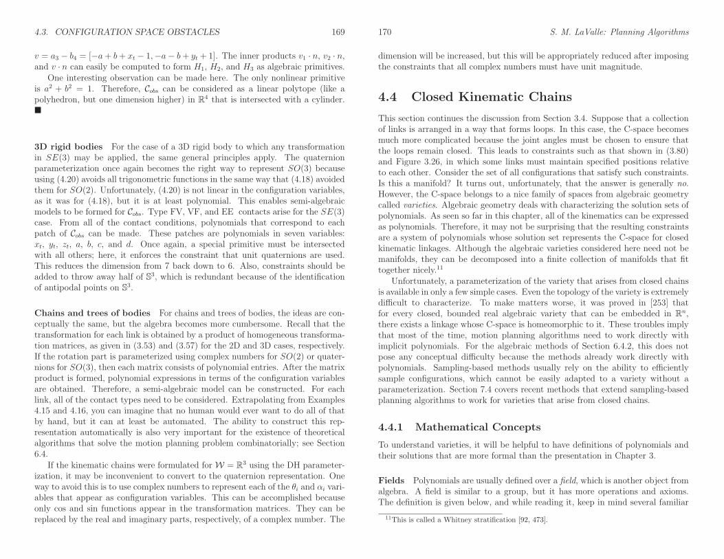
4.3. CONFIGURATION SPACE OBSTACLES 169
v = a3 − b4 = [−a+ b+ xt − 1,−a− b+ yt + 1]. The inner products v1 · n, v2 · n,and v · n can easily be computed to form H1, H2, and H3 as algebraic primitives.
One interesting observation can be made here. The only nonlinear primitiveis a2 + b2 = 1. Therefore, Cobs can be considered as a linear polytope (like apolyhedron, but one dimension higher) in R4 that is intersected with a cylinder.
3D rigid bodies For the case of a 3D rigid body to which any transformationin SE(3) may be applied, the same general principles apply. The quaternionparameterization once again becomes the right way to represent SO(3) becauseusing (4.20) avoids all trigonometric functions in the same way that (4.18) avoidedthem for SO(2). Unfortunately, (4.20) is not linear in the configuration variables,as it was for (4.18), but it is at least polynomial. This enables semi-algebraicmodels to be formed for Cobs. Type FV, VF, and EE contacts arise for the SE(3)case. From all of the contact conditions, polynomials that correspond to eachpatch of Cobs can be made. These patches are polynomials in seven variables:xt, yt, zt, a, b, c, and d. Once again, a special primitive must be intersectedwith all others; here, it enforces the constraint that unit quaternions are used.This reduces the dimension from 7 back down to 6. Also, constraints should beadded to throw away half of S3, which is redundant because of the identificationof antipodal points on S3.
Chains and trees of bodies For chains and trees of bodies, the ideas are con-ceptually the same, but the algebra becomes more cumbersome. Recall that thetransformation for each link is obtained by a product of homogeneous transforma-tion matrices, as given in (3.53) and (3.57) for the 2D and 3D cases, respectively.If the rotation part is parameterized using complex numbers for SO(2) or quater-nions for SO(3), then each matrix consists of polynomial entries. After the matrixproduct is formed, polynomial expressions in terms of the configuration variablesare obtained. Therefore, a semi-algebraic model can be constructed. For eachlink, all of the contact types need to be considered. Extrapolating from Examples4.15 and 4.16, you can imagine that no human would ever want to do all of thatby hand, but it can at least be automated. The ability to construct this rep-resentation automatically is also very important for the existence of theoreticalalgorithms that solve the motion planning problem combinatorially; see Section6.4.
If the kinematic chains were formulated for W = R3 using the DH parameter-ization, it may be inconvenient to convert to the quaternion representation. Oneway to avoid this is to use complex numbers to represent each of the θi and αi vari-ables that appear as configuration variables. This can be accomplished becauseonly cos and sin functions appear in the transformation matrices. They can bereplaced by the real and imaginary parts, respectively, of a complex number. The
170 S. M. LaValle: Planning Algorithms
dimension will be increased, but this will be appropriately reduced after imposingthe constraints that all complex numbers must have unit magnitude.
4.4 Closed Kinematic Chains
This section continues the discussion from Section 3.4. Suppose that a collectionof links is arranged in a way that forms loops. In this case, the C-space becomesmuch more complicated because the joint angles must be chosen to ensure thatthe loops remain closed. This leads to constraints such as that shown in (3.80)and Figure 3.26, in which some links must maintain specified positions relativeto each other. Consider the set of all configurations that satisfy such constraints.Is this a manifold? It turns out, unfortunately, that the answer is generally no.However, the C-space belongs to a nice family of spaces from algebraic geometrycalled varieties. Algebraic geometry deals with characterizing the solution sets ofpolynomials. As seen so far in this chapter, all of the kinematics can be expressedas polynomials. Therefore, it may not be surprising that the resulting constraintsare a system of polynomials whose solution set represents the C-space for closedkinematic linkages. Although the algebraic varieties considered here need not bemanifolds, they can be decomposed into a finite collection of manifolds that fittogether nicely.11
Unfortunately, a parameterization of the variety that arises from closed chainsis available in only a few simple cases. Even the topology of the variety is extremelydifficult to characterize. To make matters worse, it was proved in [253] thatfor every closed, bounded real algebraic variety that can be embedded in Rn,there exists a linkage whose C-space is homeomorphic to it. These troubles implythat most of the time, motion planning algorithms need to work directly withimplicit polynomials. For the algebraic methods of Section 6.4.2, this does notpose any conceptual difficulty because the methods already work directly withpolynomials. Sampling-based methods usually rely on the ability to efficientlysample configurations, which cannot be easily adapted to a variety without aparameterization. Section 7.4 covers recent methods that extend sampling-basedplanning algorithms to work for varieties that arise from closed chains.
4.4.1 Mathematical Concepts
To understand varieties, it will be helpful to have definitions of polynomials andtheir solutions that are more formal than the presentation in Chapter 3.
Fields Polynomials are usually defined over a field, which is another object fromalgebra. A field is similar to a group, but it has more operations and axioms.The definition is given below, and while reading it, keep in mind several familiar
11This is called a Whitney stratification [92, 473].
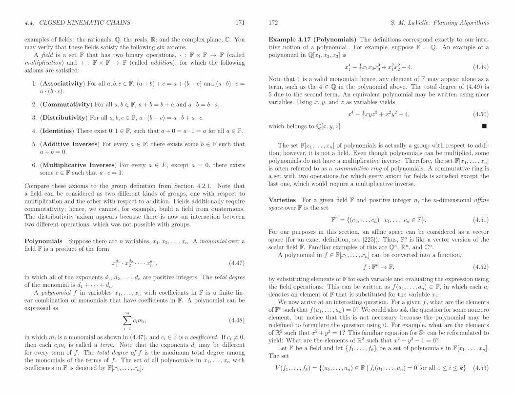
4.4. CLOSED KINEMATIC CHAINS 171
examples of fields: the rationals, Q; the reals, R; and the complex plane, C. Youmay verify that these fields satisfy the following six axioms.
A field is a set F that has two binary operations, · : F × F → F (calledmultiplication) and + : F × F → F (called addition), for which the followingaxioms are satisfied:
1. (Associativity) For all a, b, c ∈ F, (a+ b) + c = a+ (b+ c) and (a · b) · c =a · (b · c).
2. (Commutativity) For all a, b ∈ F, a+ b = b+ a and a · b = b · a.
3. (Distributivity) For all a, b, c ∈ F, a · (b+ c) = a · b+ a · c.
4. (Identities) There exist 0, 1 ∈ F, such that a+ 0 = a · 1 = a for all a ∈ F.
5. (Additive Inverses) For every a ∈ F, there exists some b ∈ F such thata+ b = 0.
6. (Multiplicative Inverses) For every a ∈ F , except a = 0, there existssome c ∈ F such that a · c = 1.
Compare these axioms to the group definition from Section 4.2.1. Note thata field can be considered as two different kinds of groups, one with respect tomultiplication and the other with respect to addition. Fields additionally requirecommutativity; hence, we cannot, for example, build a field from quaternions.The distributivity axiom appears because there is now an interaction betweentwo different operations, which was not possible with groups.
Polynomials Suppose there are n variables, x1, x2, . . . , xn. A monomial over afield F is a product of the form
xd11 · xd22 · · · · xdnn , (4.47)
in which all of the exponents d1, d2, . . ., dn are positive integers. The total degreeof the monomial is d1 + · · ·+ dn.
A polynomial f in variables x1, . . . , xn with coefficients in F is a finite lin-ear combination of monomials that have coefficients in F. A polynomial can beexpressed as
m∑
i=1
cimi, (4.48)
in which mi is a monomial as shown in (4.47), and ci ∈ F is a coefficient. If ci 6= 0,then each cimi is called a term. Note that the exponents di may be differentfor every term of f . The total degree of f is the maximum total degree amongthe monomials of the terms of f . The set of all polynomials in x1, . . . , xn withcoefficients in F is denoted by F[x1, . . . , xn].
172 S. M. LaValle: Planning Algorithms
Example 4.17 (Polynomials) The definitions correspond exactly to our intu-itive notion of a polynomial. For example, suppose F = Q. An example of apolynomial in Q[x1, x2, x3] is
x41 − 12x1x2x
33 + x21x
22 + 4. (4.49)
Note that 1 is a valid monomial; hence, any element of F may appear alone as aterm, such as the 4 ∈ Q in the polynomial above. The total degree of (4.49) is5 due to the second term. An equivalent polynomial may be written using nicervariables. Using x, y, and z as variables yields
x4 − 12xyz3 + x2y2 + 4, (4.50)
which belongs to Q[x, y, z].
The set F[x1, . . . , xn] of polynomials is actually a group with respect to addi-tion; however, it is not a field. Even though polynomials can be multiplied, somepolynomials do not have a multiplicative inverse. Therefore, the set F[x1, . . . , xn]is often referred to as a commutative ring of polynomials. A commutative ring isa set with two operations for which every axiom for fields is satisfied except thelast one, which would require a multiplicative inverse.
Varieties For a given field F and positive integer n, the n-dimensional affinespace over F is the set
Fn = (c1, . . . , cn) | c1, . . . , cn ∈ F. (4.51)
For our purposes in this section, an affine space can be considered as a vectorspace (for an exact definition, see [225]). Thus, Fn is like a vector version of thescalar field F. Familiar examples of this are Qn, Rn, and Cn.
A polynomial in f ∈ F[x1, . . . , xn] can be converted into a function,
f : Fn → F, (4.52)
by substituting elements of F for each variable and evaluating the expression usingthe field operations. This can be written as f(a1, . . . , an) ∈ F, in which each aidenotes an element of F that is substituted for the variable xi.
We now arrive at an interesting question. For a given f , what are the elementsof Fn such that f(a1, . . . , an) = 0? We could also ask the question for some nonzeroelement, but notice that this is not necessary because the polynomial may beredefined to formulate the question using 0. For example, what are the elementsof R2 such that x2 + y2 = 1? This familiar equation for S1 can be reformulated toyield: What are the elements of R2 such that x2 + y2 − 1 = 0?
Let F be a field and let f1, . . . , fk be a set of polynomials in F[x1, . . . , xn].The set
V (f1, . . . , fk) = (a1, . . . , an) ∈ F | fi(a1, . . . , an) = 0 for all 1 ≤ i ≤ k (4.53)

4.4. CLOSED KINEMATIC CHAINS 173
is called the (affine) variety defined by f1, . . . , fk. One interesting fact is thatunions and intersections of varieties are varieties. Therefore, they behave like thesemi-algebraic sets from Section 3.1.2, but for varieties only equality constraintsare allowed. Consider the varieties V (f1, . . . , fk) and V (g1, . . . , gl). Their inter-section is given by
V (f1, . . . , fk) ∩ V (g1, . . . , gl) = V (f1, . . . , fk, g1, . . . , gl), (4.54)
because each element of Fn must produce a 0 value for each of the polynomials inf1, . . . , fk, g1, . . . , gl.
To obtain unions, the polynomials simply need to be multiplied. For example,consider the varieties V1, V2 ⊂ F defined as
V1 = (a1, . . . , an) ∈ F | f1(a1, . . . , an) = 0 (4.55)
and
V2 = (a1, . . . , an) ∈ F | f2(a1, . . . , an) = 0. (4.56)
The set V1 ∪ V2 ⊂ F is obtained by forming the polynomial f = f1f2. Note thatf(a1, . . . , an) = 0 if either f1(a1, . . . , an) = 0 or f2(a1, . . . , an) = 0. Therefore,V1∪V2 is a variety. The varieties V1 and V2 were defined using a single polynomial,but the same idea applies to any variety. All pairs of the form figj must appearin the argument of V (·) if there are multiple polynomials.
4.4.2 Kinematic Chains in R2
To illustrate the concepts it will be helpful to study a simple case in detail. LetW = R2, and suppose there is a chain of links, A1, . . ., An, as considered inExample 3.3 for n = 3. Suppose that the first link is attached at the origin ofW by a revolute joint, and every other link, Ai is attached to Ai−1 by a revolutejoint. This yields the C-space
C = S1 × S1 × · · · × S1 = Tn, (4.57)
which is the n-dimensional torus.
Two links If there are two links, A1 and A2, then the C-space can be nicelyvisualized as a square with opposite faces identified. Each coordinate, θ1 and θ2,ranges from 0 to 2π, for which 0 ∼ 2π. Suppose that each link has length 1. Thisyields a1 = 1. A point (x, y) ∈ A2 is transformed as
cos θ1 − sin θ1 0sin θ1 cos θ1 00 0 1
cos θ2 − sin θ2 1sin θ2 cos θ2 00 0 1
xy1
. (4.58)
174 S. M. LaValle: Planning Algorithms
To obtain polynomials, the technique from Section 4.2.2 is applied to replacethe trigonometric functions using ai = cos θi and bi = sin θi, subject to the con-straint a2i + b2i = 1. This results in
a1 −b1 0b1 a1 00 0 1
a2 −b2 1b2 a2 00 0 1
xy1
, (4.59)
for which the constraints a2i + b2i = 1 for i = 1, 2 must be satisfied. This preservesthe torus topology of C, but now the C-space is embedded in R4. The coordinatesof each point are (a1, b1, a2, b2) ∈ R4; however, there are only two degrees offreedom because each ai, bi pair must lie on a unit circle.
Multiplying the matrices in (4.59) yields the polynomials, f1, f2 ∈ R[a1, b1, a2, b2],
f1 = xa1a2 − ya1b2 − xb1b2 + ya2b1 + a1 (4.60)
andf2 = −ya1a2 + xa1b2 + xa2b1 − yb1b2 + b1, (4.61)
for the x and y coordinates, respectively. Note that the polynomial variables areconfiguration parameters; x and y are not polynomial variables. For a given point(x, y) ∈ A2, all coefficients are determined.
A zero-dimensional variety Now a kinematic closure constraint will be im-posed. Fix the point (1, 0) in the body frame of A2 at (1, 1) in W . This yieldsthe constraints
f1 = a1a2 − b1b2 + a1 = 1 (4.62)
andf2 = a1b2 + a2b1 + b1 = 1, (4.63)
by substituting x = 1 and y = 0 into (4.60) and (4.61). This yields the variety
V (a1a2 − b1b2 + a1 − 1, a1b2 + a2b1 + b1 − 1, a21 + b21 − 1, a22 + b22 − 1), (4.64)
which is a subset of R4. The polynomials are slightly modified because eachconstraint must be written in the form f = 0.
Although (4.64) represents the constrained configuration space for the chainof two links, it is not very explicit. Without an explicit characterization (i.e., aparameterization), it complicates motion planning. From Figure 4.22 it can beseen that there are only two solutions. These occur for θ1 = 0, θ2 = π/2 andθ1 = π/2, θ2 = −π/2. In terms of the polynomial variables, (a1, b1, a2, b2), thetwo solutions are (1, 0, 0, 1) and (0, 1, 0,−1). These may be substituted into eachpolynomial in (4.64) to verify that 0 is obtained. Thus, the variety represents twopoints in R4. This can also be interpreted as two points on the torus, S1 × S1.
It might not be surprising that the set of solutions has dimension zero becausethere are four independent constraints, shown in (4.64), and four variables. De-pending on the choices, the variety may be empty. For example, it is physicallyimpossible to bring the point (1, 0) ∈ A2 to (1000, 0) ∈ W .

4.4. CLOSED KINEMATIC CHAINS 175
A1
A2
y1
x1
p
Figure 4.22: Two configurations hold the point p at (1, 1).
A one-dimensional variety The most interesting and complicated situationsoccur when there is a continuum of solutions. For example, if one of the constraintsis removed, then a one-dimensional set of solutions can be obtained. Suppose onlyone variable is constrained for the example in Figure 4.22. Intuitively, this shouldyield a one-dimensional variety. Set the x coordinate to 0, which yields
a1a2 − b1b2 + a1 = 0, (4.65)
and allow any possible value for y. As shown in Figure 4.23a, the point p must fol-low the y-axis. (This is equivalent to a three-bar linkage that can be constructedby making a third joint that is prismatic and forced to stay along the y-axis.)Figure 4.23b shows the resulting variety V (a1a2− b1b2+ a1) but plotted in θ1− θ2coordinates to reduce the dimension from 4 to 2 for visualization purposes. Tocorrectly interpret the figures in Figure 4.23, recall that the topology is S1 × S1,which means that the top and bottom are identified, and also the sides are identi-fied. The center of Figure 4.23b, which corresponds to (θ1, θ2) = (π, π), preventsthe variety from being a manifold. The resulting space is actually homeomorphicto two circles that touch at a point. Thus, even with such a simple example,the nice manifold structure may disappear. Observe that at (π, π) the links arecompletely overlapped, and the point p of A2 is placed at (0, 0) in W . The hori-zontal line in Figure 4.23b corresponds to keeping the two links overlapping andswinging them around together by varying θ1. The diagonal lines correspond tomoving along configurations such as the one shown in Figure 4.23a. Note that thelinks and the y-axis always form an isosceles triangle, which can be used to showthat the solution set is any pair of angles, θ1, θ2 for which θ2 = π − θ1. This isthe reason why the diagonal curves in Figure 4.23b are linear. Figures 4.23c and
176 S. M. LaValle: Planning Algorithms
4.23d show the varieties for the constraints
a1a2 − b1b2 + a1 =18, (4.66)
anda1a2 − b1b2 + a1 = 1, (4.67)
respectively. In these cases, the point (0, 1) in A2 must follow the x = 1/8 andx = 1 axes, respectively. The varieties are manifolds, which are homeomorphicto S1. The sequence from Figure 4.23b to 4.23d can be imagined as part of ananimation in which the variety shrinks into a small circle. Eventually, it shrinksto a point for the case a1a2 − b1b2 + a1 = 2, because the only solution is whenθ1 = θ2 = 0. Beyond this, the variety is the empty set because there are nosolutions. Thus, by allowing one constraint to vary, four different topologies areobtained: 1) two circles joined at a point, 2) a circle, 3) a point, and 4) the emptyset.
Three links Since visualization is still possible with one more dimension, sup-pose there are three links, A1, A2, and A3. The C-space can be visualized as a3D cube with opposite faces identified. Each coordinate θi ranges from 0 to 2π,for which 0 ∼ 2π. Suppose that each link has length 1 to obtain a1 = a2 = 1. Apoint (x, y) ∈ A3 is transformed as
cos θ1 − sin θ1 0sin θ1 cos θ1 00 0 1
cos θ2 − sin θ2 10sin θ2 cos θ2 00 0 1
cos θ3 − sin θ3 10sin θ3 cos θ3 00 0 1
xy1
.
(4.68)To obtain polynomials, let ai = cos θi and bi = sin θi, which results in
a1 −b1 0b1 a1 00 0 1
a2 −b2 1b2 a2 00 0 1
a3 −b3 1b3 a3 00 0 1
xy1
, (4.69)
for which the constraints a2i + b2i = 1 for i = 1, 2, 3 must also be satisfied. Thispreserves the torus topology of C, but now it is embedded in R6. Multiplying thematrices yields the polynomials f1, f2 ∈ R[a1, b1, a2, b2, a3, b3], defined as
f1 = 2a1a2a3 − a1b2b3 + a1a2 − 2b1b2a3 − b1a2b3 + a1, (4.70)
andf2 = 2b1a2a3 − b1b2b3 + b1a2 + 2a1b2a3 + a1a2b3, (4.71)
for the x and y coordinates, respectively.Again, consider imposing a single constraint,
2a1a2a3 − a1b2b3 + a1a2 − 2b1b2a3 − b1a2b3 + a1 = 0, (4.72)
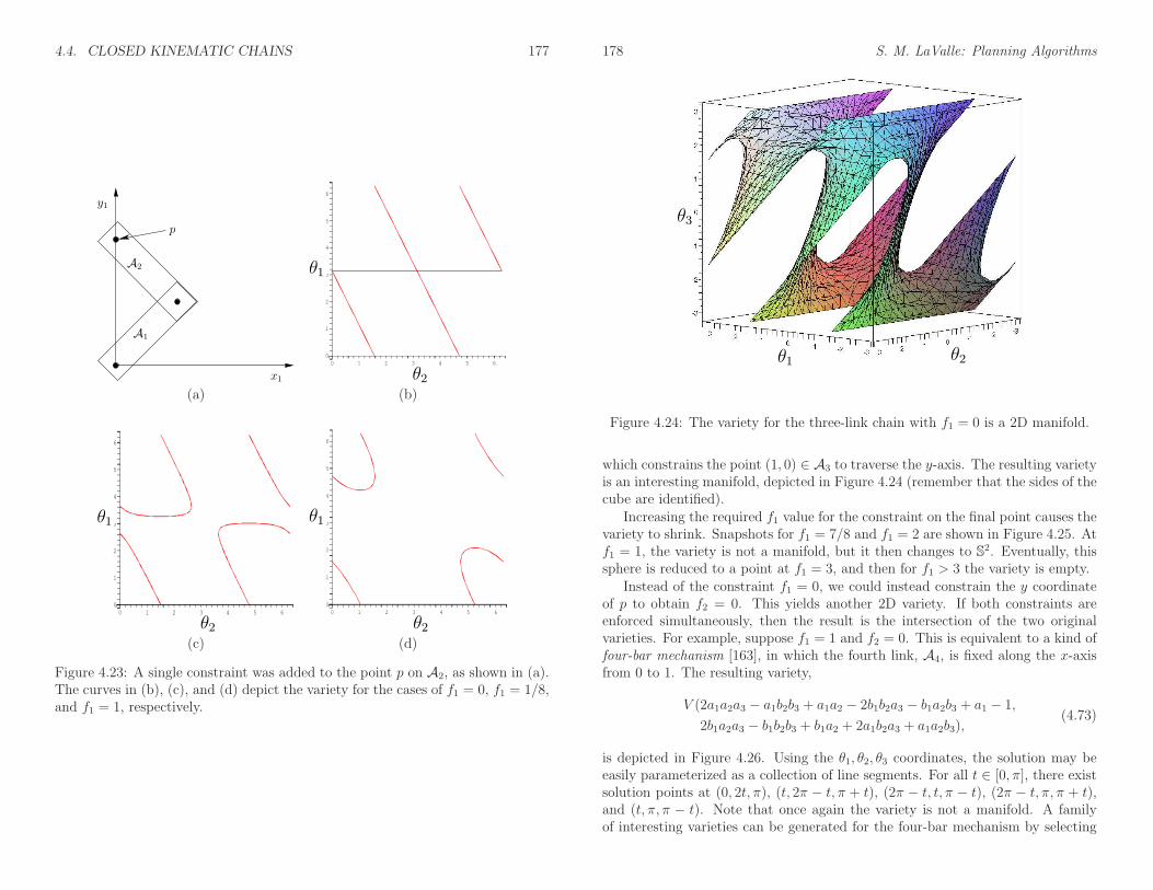
4.4. CLOSED KINEMATIC CHAINS 177
A1
A2
x1
y1
p
2
theta2
5
1
10
4
2
3
0
theta1
653 4
6
θ1
θ2
(a) (b)
theta2
5
1
6
4
0
theta1
3 642 5
2
3
10
θ1
θ2
5
1
3
theta1
654320
theta2
6
4
2
01
θ1
θ2
(c) (d)
Figure 4.23: A single constraint was added to the point p on A2, as shown in (a).The curves in (b), (c), and (d) depict the variety for the cases of f1 = 0, f1 = 1/8,and f1 = 1, respectively.
178 S. M. LaValle: Planning Algorithms
θ3
θ1 θ2
Figure 4.24: The variety for the three-link chain with f1 = 0 is a 2D manifold.
which constrains the point (1, 0) ∈ A3 to traverse the y-axis. The resulting varietyis an interesting manifold, depicted in Figure 4.24 (remember that the sides of thecube are identified).
Increasing the required f1 value for the constraint on the final point causes thevariety to shrink. Snapshots for f1 = 7/8 and f1 = 2 are shown in Figure 4.25. Atf1 = 1, the variety is not a manifold, but it then changes to S2. Eventually, thissphere is reduced to a point at f1 = 3, and then for f1 > 3 the variety is empty.
Instead of the constraint f1 = 0, we could instead constrain the y coordinateof p to obtain f2 = 0. This yields another 2D variety. If both constraints areenforced simultaneously, then the result is the intersection of the two originalvarieties. For example, suppose f1 = 1 and f2 = 0. This is equivalent to a kind offour-bar mechanism [163], in which the fourth link, A4, is fixed along the x-axisfrom 0 to 1. The resulting variety,
V (2a1a2a3 − a1b2b3 + a1a2 − 2b1b2a3 − b1a2b3 + a1 − 1,
2b1a2a3 − b1b2b3 + b1a2 + 2a1b2a3 + a1a2b3),(4.73)
is depicted in Figure 4.26. Using the θ1, θ2, θ3 coordinates, the solution may beeasily parameterized as a collection of line segments. For all t ∈ [0, π], there existsolution points at (0, 2t, π), (t, 2π − t, π + t), (2π − t, t, π − t), (2π − t, π, π + t),and (t, π, π − t). Note that once again the variety is not a manifold. A familyof interesting varieties can be generated for the four-bar mechanism by selecting
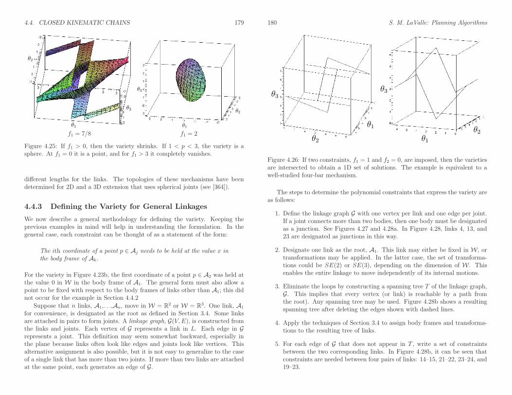
4.4. CLOSED KINEMATIC CHAINS 179
θ1
θ3
θ2
θ2
θ1
θ3
f1 = 7/8 f1 = 2
Figure 4.25: If f1 > 0, then the variety shrinks. If 1 < p < 3, the variety is asphere. At f1 = 0 it is a point, and for f1 > 3 it completely vanishes.
different lengths for the links. The topologies of these mechanisms have beendetermined for 2D and a 3D extension that uses spherical joints (see [364]).
4.4.3 Defining the Variety for General Linkages
We now describe a general methodology for defining the variety. Keeping theprevious examples in mind will help in understanding the formulation. In thegeneral case, each constraint can be thought of as a statement of the form:
The ith coordinate of a point p ∈ Aj needs to be held at the value x inthe body frame of Ak.
For the variety in Figure 4.23b, the first coordinate of a point p ∈ A2 was held atthe value 0 in W in the body frame of A1. The general form must also allow apoint to be fixed with respect to the body frames of links other than A1; this didnot occur for the example in Section 4.4.2
Suppose that n links, A1,. . .,An, move in W = R2 or W = R3. One link, A1
for convenience, is designated as the root as defined in Section 3.4. Some linksare attached in pairs to form joints. A linkage graph, G(V,E), is constructed fromthe links and joints. Each vertex of G represents a link in L. Each edge in Grepresents a joint. This definition may seem somewhat backward, especially inthe plane because links often look like edges and joints look like vertices. Thisalternative assignment is also possible, but it is not easy to generalize to the caseof a single link that has more than two joints. If more than two links are attachedat the same point, each generates an edge of G.
180 S. M. LaValle: Planning Algorithms
θ1
θ2
θ3θ3
θ2
θ1
Figure 4.26: If two constraints, f1 = 1 and f2 = 0, are imposed, then the varietiesare intersected to obtain a 1D set of solutions. The example is equivalent to awell-studied four-bar mechanism.
The steps to determine the polynomial constraints that express the variety areas follows:
1. Define the linkage graph G with one vertex per link and one edge per joint.If a joint connects more than two bodies, then one body must be designatedas a junction. See Figures 4.27 and 4.28a. In Figure 4.28, links 4, 13, and23 are designated as junctions in this way.
2. Designate one link as the root, A1. This link may either be fixed in W , ortransformations may be applied. In the latter case, the set of transforma-tions could be SE(2) or SE(3), depending on the dimension of W . Thisenables the entire linkage to move independently of its internal motions.
3. Eliminate the loops by constructing a spanning tree T of the linkage graph,G. This implies that every vertex (or link) is reachable by a path fromthe root). Any spanning tree may be used. Figure 4.28b shows a resultingspanning tree after deleting the edges shown with dashed lines.
4. Apply the techniques of Section 3.4 to assign body frames and transforma-tions to the resulting tree of links.
5. For each edge of G that does not appear in T , write a set of constraintsbetween the two corresponding links. In Figure 4.28b, it can be seen thatconstraints are needed between four pairs of links: 14–15, 21–22, 23–24, and19–23.
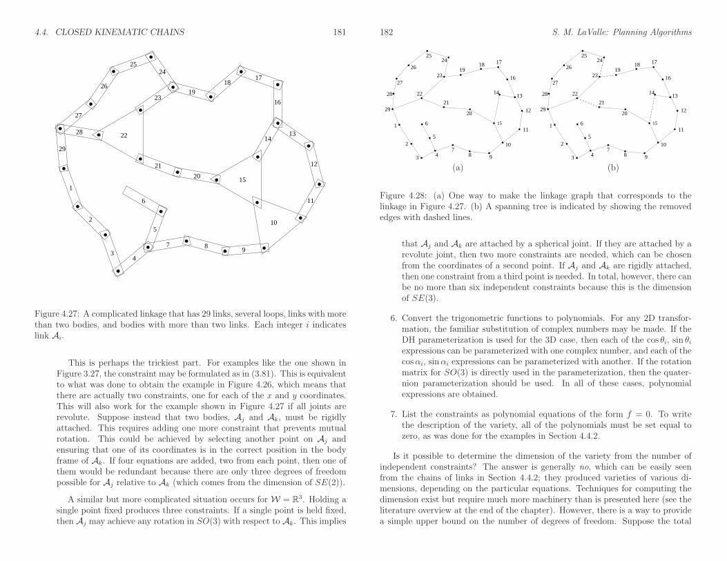
4.4. CLOSED KINEMATIC CHAINS 181
1
2
34
5
6
7 89
10
11
12
1314
15
16
1718
19
20
21
22
23
2425
26
27
28
29
Figure 4.27: A complicated linkage that has 29 links, several loops, links with morethan two bodies, and bodies with more than two links. Each integer i indicateslink Ai.
This is perhaps the trickiest part. For examples like the one shown inFigure 3.27, the constraint may be formulated as in (3.81). This is equivalentto what was done to obtain the example in Figure 4.26, which means thatthere are actually two constraints, one for each of the x and y coordinates.This will also work for the example shown in Figure 4.27 if all joints arerevolute. Suppose instead that two bodies, Aj and Ak, must be rigidlyattached. This requires adding one more constraint that prevents mutualrotation. This could be achieved by selecting another point on Aj andensuring that one of its coordinates is in the correct position in the bodyframe of Ak. If four equations are added, two from each point, then one ofthem would be redundant because there are only three degrees of freedompossible for Aj relative to Ak (which comes from the dimension of SE(2)).
A similar but more complicated situation occurs for W = R3. Holding asingle point fixed produces three constraints. If a single point is held fixed,then Aj may achieve any rotation in SO(3) with respect to Ak. This implies
182 S. M. LaValle: Planning Algorithms
27
22
21
1918
14
17
12
11
10
987
5
15
13
16
2425
23
26
28
29
1
2
3
20
6
4
27
22
21
1918
14
17
12
11
10
987
5
15
13
16
24
23
26
28
29
1
2
3
20
6
4
25
(a) (b)
Figure 4.28: (a) One way to make the linkage graph that corresponds to thelinkage in Figure 4.27. (b) A spanning tree is indicated by showing the removededges with dashed lines.
that Aj and Ak are attached by a spherical joint. If they are attached by arevolute joint, then two more constraints are needed, which can be chosenfrom the coordinates of a second point. If Aj and Ak are rigidly attached,then one constraint from a third point is needed. In total, however, there canbe no more than six independent constraints because this is the dimensionof SE(3).
6. Convert the trigonometric functions to polynomials. For any 2D transfor-mation, the familiar substitution of complex numbers may be made. If theDH parameterization is used for the 3D case, then each of the cos θi, sin θiexpressions can be parameterized with one complex number, and each of thecosαi, sinαi expressions can be parameterized with another. If the rotationmatrix for SO(3) is directly used in the parameterization, then the quater-nion parameterization should be used. In all of these cases, polynomialexpressions are obtained.
7. List the constraints as polynomial equations of the form f = 0. To writethe description of the variety, all of the polynomials must be set equal tozero, as was done for the examples in Section 4.4.2.
Is it possible to determine the dimension of the variety from the number ofindependent constraints? The answer is generally no, which can be easily seenfrom the chains of links in Section 4.4.2; they produced varieties of various di-mensions, depending on the particular equations. Techniques for computing thedimension exist but require much more machinery than is presented here (see theliterature overview at the end of the chapter). However, there is a way to providea simple upper bound on the number of degrees of freedom. Suppose the total

4.4. CLOSED KINEMATIC CHAINS 183
degrees of freedom of the linkage in spanning tree form is m. Each independentconstraint can remove at most one degree of freedom. Thus, if there are l inde-pendent constraints, then the variety can have no more than m − l dimensions.One expression of this for a general class of mechanisms is the Kutzbach criterion;the planar version of this is called Grubler’s formula [163].
One final concern is the obstacle region, Cobs. Once the variety has been identi-fied, the obstacle region and motion planning definitions in (4.34) and Formulation4.1 do not need to be changed. The configuration space C must be redefined, how-ever, to be the set of configurations that satisfy the closure constraints.
Further Reading
Section 4.1 introduced the basic definitions and concepts of topology. Further studyof this fascinating subject can provide a much deeper understanding of configurationspaces. There are many books on topology, some of which may be intimidating, de-pending on your level of math training. For a heavily illustrated, gentle introductionto topology, see [281]. Another gentle introduction appears in [256]. An excellent textat the graduate level is available on-line: [226]. Other sources include [30, 232]. Tounderstand the motivation for many technical definitions in topology, [449] is helpful.The manifold coverage in Section 4.1.2 was simpler than that found in most sourcesbecause most sources introduce smooth manifolds, which are complicated by differentia-bility requirements (these were not needed in this chapter); see Section 8.3.2 for smoothmanifolds. For the configuration spaces of points moving on a topological graph, see [3].
Section 4.2 provided basic C-space definitions. For further reading on matrix groupsand their topological properties, see [45], which provides a transition into more advancedmaterial on Lie group theory. For more about quaternions in engineering, see [113, 294].The remainder of Section 4.2 and most of Section 4.3 were inspired by the coverage in[304]. C-spaces are also covered in [118]. For further reading on computing represen-tations of Cobs, see [262, 380] for bitmaps, and Chapter 6 and [435] for combinatorialapproaches.
Much of the presentation in Section 4.4 was inspired by the nice introduction to alge-braic varieties in [138], which even includes robotics examples; methods for determiningthe dimension of a variety are also covered. More algorithmic coverage appears in [369].See [360] for detailed coverage of robots that are designed with closed kinematic chains.
Exercises
1. Consider the set X = 1, 2, 3, 4, 5. Let X, ∅, 1, 3, 1, 2, 2, 3, 1, 2, and3 be the collection of all subsets of X that are designated as open sets.
(a) Is X a topological space?
(b) Is it a topological space if 1, 2, 3 is added to the collection of open sets?Explain.
(c) What are the closed sets (assuming 1, 2, 3 is included as an open set)?
(d) Are any subsets of X neither open nor closed?
184 S. M. LaValle: Planning Algorithms
2. Continuous functions for the strange topology:
(a) Give an example of a continuous function, f : X → X, for the strangetopology in Example 4.4.
(b) Characterize the set of all possible continuous functions.
3. For the letters of the Russian alphabet, A, B, V, G, D, E, E, Ж, Z, I, I,K, L, M, N, O, P, R, S, T, U, F, H, C, Q, X, W, Ъ, Y, Ь, З, ,, determine which pairs are homeomorphic. Imagine each as a 1D subset of R2
and draw them accordingly before solving the problem.
4. Prove that homeomorphisms yield an equivalence relation on the collection of alltopological spaces.
5. What is the dimension of the C-space for a cylindrical rod that can translate androtate in R3? If the rod is rotated about its central axis, it is assumed that therod’s position and orientation are not changed in any detectable way. Expressthe C-space of the rod in terms of a Cartesian product of simpler spaces (such asS1, S2, Rn, P 2, etc.). What is your reasoning?
6. Let τ1 : [0, 1] → R2 be a loop path that traverses the unit circle in the plane,defined as τ1(s) = (cos(2πs), sin(2πs)). Let τ2 : [0, 1] → R2 be another looppath: τ1(s) = (−2 + 3 cos(2πs), 12 sin(2πs)). This path traverses an ellipse thatis centered at (−2, 0). Show that τ1 and τ2 are homotopic (by constructing acontinuous function with an additional parameter that “morphs” τ1 into τ2).
7. Prove that homotopy yields an equivalence relation on the set of all paths fromsome x1 ∈ X to some x2 ∈ X, in which x1 and x2 may be chosen arbitrarily.
8. Determine the C-space for a spacecraft that can translate and rotate in a 2DAsteroids-style video game. The sides of the screen are identified. The top andbottom are also identified. There are no “twists” in the identifications.
9. Repeat the derivation of HA from Section 4.3.3, but instead consider Type VEcontacts.
10. Determine the C-space for a car that drives around on a huge sphere (such asthe earth with no mountains or oceans). Assume the sphere is big enough sothat its curvature may be neglected (e.g., the car rests flatly on the earth withoutwobbling). [Hint: It is not S2 × S1.]
11. Suppose that A and O are each defined as equilateral triangles, with coordinates(0, 0), (2, 0), and (1,
√3). Determine the C-space obstacle. Specify the coordinates
of all of its vertices and indicate the corresponding contact type for each edge.
12. Show that (4.20) is a valid rotation matrix for all unit quaternions.
13. Show that F[x1, . . . , xn], the set of polynomials over a field F with variablesx1, . . . , xn, is a group with respect to addition.
14. Quaternions:
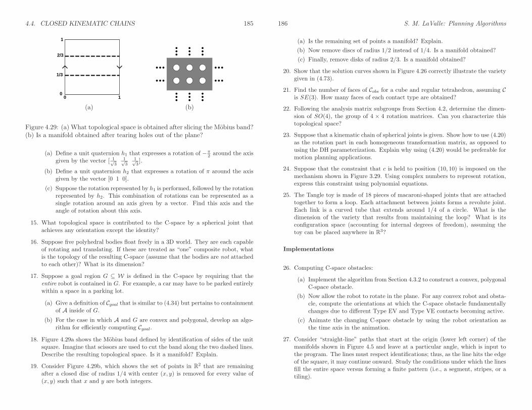
4.4. CLOSED KINEMATIC CHAINS 185
0 10
1/3
2/3
1
(a) (b)
Figure 4.29: (a) What topological space is obtained after slicing the Mobius band?(b) Is a manifold obtained after tearing holes out of the plane?
(a) Define a unit quaternion h1 that expresses a rotation of −π2 around the axis
given by the vector [ 1√3
1√3
1√3].
(b) Define a unit quaternion h2 that expresses a rotation of π around the axisgiven by the vector [0 1 0].
(c) Suppose the rotation represented by h1 is performed, followed by the rotationrepresented by h2. This combination of rotations can be represented as asingle rotation around an axis given by a vector. Find this axis and theangle of rotation about this axis.
15. What topological space is contributed to the C-space by a spherical joint thatachieves any orientation except the identity?
16. Suppose five polyhedral bodies float freely in a 3D world. They are each capableof rotating and translating. If these are treated as “one” composite robot, whatis the topology of the resulting C-space (assume that the bodies are not attachedto each other)? What is its dimension?
17. Suppose a goal region G ⊆ W is defined in the C-space by requiring that theentire robot is contained in G. For example, a car may have to be parked entirelywithin a space in a parking lot.
(a) Give a definition of Cgoal that is similar to (4.34) but pertains to containmentof A inside of G.
(b) For the case in which A and G are convex and polygonal, develop an algo-rithm for efficiently computing Cgoal.
18. Figure 4.29a shows the Mobius band defined by identification of sides of the unitsquare. Imagine that scissors are used to cut the band along the two dashed lines.Describe the resulting topological space. Is it a manifold? Explain.
19. Consider Figure 4.29b, which shows the set of points in R2 that are remainingafter a closed disc of radius 1/4 with center (x, y) is removed for every value of(x, y) such that x and y are both integers.
186 S. M. LaValle: Planning Algorithms
(a) Is the remaining set of points a manifold? Explain.
(b) Now remove discs of radius 1/2 instead of 1/4. Is a manifold obtained?
(c) Finally, remove disks of radius 2/3. Is a manifold obtained?
20. Show that the solution curves shown in Figure 4.26 correctly illustrate the varietygiven in (4.73).
21. Find the number of faces of Cobs for a cube and regular tetrahedron, assuming Cis SE(3). How many faces of each contact type are obtained?
22. Following the analysis matrix subgroups from Section 4.2, determine the dimen-sion of SO(4), the group of 4 × 4 rotation matrices. Can you characterize thistopological space?
23. Suppose that a kinematic chain of spherical joints is given. Show how to use (4.20)as the rotation part in each homogeneous transformation matrix, as opposed tousing the DH parameterization. Explain why using (4.20) would be preferable formotion planning applications.
24. Suppose that the constraint that c is held to position (10, 10) is imposed on themechanism shown in Figure 3.29. Using complex numbers to represent rotation,express this constraint using polynomial equations.
25. The Tangle toy is made of 18 pieces of macaroni-shaped joints that are attachedtogether to form a loop. Each attachment between joints forms a revolute joint.Each link is a curved tube that extends around 1/4 of a circle. What is thedimension of the variety that results from maintaining the loop? What is itsconfiguration space (accounting for internal degrees of freedom), assuming thetoy can be placed anywhere in R3?
Implementations
26. Computing C-space obstacles:
(a) Implement the algorithm from Section 4.3.2 to construct a convex, polygonalC-space obstacle.
(b) Now allow the robot to rotate in the plane. For any convex robot and obsta-cle, compute the orientations at which the C-space obstacle fundamentallychanges due to different Type EV and Type VE contacts becoming active.
(c) Animate the changing C-space obstacle by using the robot orientation asthe time axis in the animation.
27. Consider “straight-line” paths that start at the origin (lower left corner) of themanifolds shown in Figure 4.5 and leave at a particular angle, which is input tothe program. The lines must respect identifications; thus, as the line hits the edgeof the square, it may continue onward. Study the conditions under which the linesfill the entire space versus forming a finite pattern (i.e., a segment, stripes, or atiling).

Chapter 5
Sampling-Based Motion Planning
There are two main philosophies for addressing the motion planning problem, inFormulation 4.1 from Section 4.3.1. This chapter presents one of the philosophies,sampling-based motion planning, which is outlined in Figure 5.1. The main idea isto avoid the explicit construction of Cobs, as described in Section 4.3, and insteadconduct a search that probes the C-space with a sampling scheme. This probingis enabled by a collision detection module, which the motion planning algorithmconsiders as a “black box.” This enables the development of planning algorithmsthat are independent of the particular geometric models. The collision detectionmodule handles concerns such as whether the models are semi-algebraic sets, 3Dtriangles, nonconvex polyhedra, and so on. This general philosophy has been verysuccessful in recent years for solving problems from robotics, manufacturing, andbiological applications that involve thousands and even millions of geometric prim-itives. Such problems would be practically impossible to solve using techniquesthat explicitly represent Cobs.
Notions of completeness It is useful to define several notions of completenessfor sampling-based algorithms. These algorithms have the drawback that theyresult in weaker guarantees that the problem will be solved. An algorithm isconsidered complete if for any input it correctly reports whether there is a solu-
Sampling−BasedMotion Planning AlgorithmCollision
DetectionGeometricModels
DiscreteSearching
C−SpaceSampling
Figure 5.1: The sampling-based planning philosophy uses collision detection asa “black box” that separates the motion planning from the particular geometricand kinematic models. C-space sampling and discrete planning (i.e., searching)are performed.
187
188 S. M. LaValle: Planning Algorithms
tion in a finite amount of time. If a solution exists, it must return one in finitetime. The combinatorial motion planning methods of Chapter 6 will achieve this.Unfortunately, such completeness is not achieved with sampling-based planning.Instead, weaker notions of completeness are tolerated. The notion of densenessbecomes important, which means that the samples come arbitrarily close to anyconfiguration as the number of iterations tends to infinity. A deterministic ap-proach that samples densely will be called resolution complete. This means thatif a solution exists, the algorithm will find it in finite time; however, if a solutiondoes not exist, the algorithm may run forever. Many sampling-based approachesare based on random sampling, which is dense with probability one. This leadsto algorithms that are probabilistically complete, which means that with enoughpoints, the probability that it finds an existing solution converges to one. Themost relevant information, however, is the rate of convergence, which is usuallyvery difficult to establish.
Section 5.1 presents metric and measure space concepts, which are funda-mental to nearly all sampling-based planning algorithms. Section 5.2 presentsgeneral sampling concepts and quality criteria that are effective for analyzing theperformance of sampling-based algorithms. Section 5.3 gives a brief overview ofcollision detection algorithms, to gain an understanding of the information avail-able to a planning algorithm and the computation price that must be paid toobtain it. Section 5.4 presents a framework that defines algorithms which solvemotion planning problems by integrating sampling and discrete planning (i.e.,searching) techniques. These approaches can be considered single query in thesense that a single pair, (qI , qG), is given, and the algorithm must search until itfinds a solution (or it may report early failure). Section 5.5 focuses on rapidlyexploring random trees (RRTs) and rapidly exploring dense trees (RDTs), whichare used to develop efficient single-query planning algorithms. Section 5.6 coversmultiple-query algorithms, which invest substantial preprocessing effort to build adata structure that is later used to obtain efficient solutions for many initial-goalpairs. In this case, it is assumed that the obstacle region O remains the same forevery query.
5.1 Distance and Volume in C-Space
Virtually all sampling-based planning algorithms require a function that measuresthe distance between two points in C. In most cases, this results in a metricspace, which is introduced in Section 5.1.1. Useful examples for motion planningare given in Section 5.1.2. It will also be important in many of these algorithmsto define the volume of a subset of C. This requires a measure space, which isintroduced in Section 5.1.3. Section 5.1.4 introduces invariant measures, whichshould be used whenever possible.

5.1. DISTANCE AND VOLUME IN C-SPACE 189
5.1.1 Metric Spaces
It is straightforward to define Euclidean distance in Rn. To define a distancefunction over any C, however, certain axioms will have to be satisfied so that itcoincides with our expectations based on Euclidean distance.
The following definition and axioms are used to create a function that convertsa topological space into a metric space.1 A metric space (X, ρ) is a topologicalspace X equipped with a function ρ : X ×X → R such that for any a, b, c ∈ X:
1. Nonnegativity: ρ(a, b) ≥ 0.
2. Reflexivity: ρ(a, b) = 0 if and only if a = b.
3. Symmetry: ρ(a, b) = ρ(b, a).
4. Triangle inequality: ρ(a, b) + ρ(b, c) ≥ ρ(a, c).
The function ρ defines distances between points in the metric space, and eachof the four conditions on ρ agrees with our intuitions about distance. The finalcondition implies that ρ is optimal in the sense that the distance from a to c willalways be less than or equal to the total distance obtained by traveling throughan intermediate point b on the way from a to c.
Lp metrics The most important family of metrics over Rn is given for any p ≥ 1as
ρ(x, x′) =
( n∑
i=1
|xi − x′i|p)1/p
. (5.1)
For each value of p, (5.1) is called an Lp metric (pronounced “el pee”). The threemost common cases are
1. L2: The Euclidean metric, which is the familiar Euclidean distance in Rn.
2. L1: The Manhattan metric, which is often nicknamed this way because inR2 it corresponds to the length of a path that is obtained by moving alongan axis-aligned grid. For example, the distance from (0, 0) to (2, 5) is 7 bytraveling “east two blocks” and then “north five blocks”.
3. L∞: The L∞ metric must actually be defined by taking the limit of (5.1) asp tends to infinity. The result is
L∞(x, x′) = max1≤i≤n
|xi − x′i|, (5.2)
which seems correct because the larger the value of p, the more the largestterm of the sum in (5.1) dominates.
1Some topological spaces are notmetrizable, which means that no function exists that satisfiesthe axioms. Many metrization theorems give sufficient conditions for a topological space to bemetrizable [232], and virtually any space that has arisen in motion planning will be metrizable.
190 S. M. LaValle: Planning Algorithms
An Lp metric can be derived from a norm on a vector space. An Lp norm overRn is defined as
‖x‖p =( n∑
i=1
|xi|p)1/p
. (5.3)
The case of p = 2 is the familiar definition of the magnitude of a vector, which iscalled the Euclidean norm. For example, assume the vector space is Rn, and let‖ · ‖ be the standard Euclidean norm. The L2 metric is ρ(x, y) = ‖x − y‖. AnyLp metric can be written in terms of a vector subtraction, which is notationallyconvenient.
Metric subspaces By verifying the axioms, it can be shown that any subspaceY ⊂ X of a metric space (X, ρ) itself becomes a metric space by restricting thedomain of ρ to Y ×Y . This conveniently provides metrics on any of the manifoldsand varieties from Chapter 4 by simply using any Lp metric on Rm, the space inwhich the manifold or variety is embedded.
Cartesian products of metric spaces Metrics extend nicely across Cartesianproducts, which is very convenient because C-spaces are often constructed fromCartesian products, especially in the case of multiple bodies. Let (X, ρx) and(Y, ρy) be two metric spaces. A metric space (Z, ρz) can be constructed for theCartesian product Z = X × Y by defining the metric ρz as
ρz(z, z′) = ρz(x, y, x
′, y′) = c1ρx(x, x′) + c2ρy(y, y
′), (5.4)
in which c1 > 0 and c2 > 0 are any positive real constants, and x, x′ ∈ X andy, y′ ∈ Y . Each z ∈ Z is represented as z = (x, y).
Other combinations lead to a metric for Z; for example,
ρz(z, z′) =
(
c1[
ρx(x, x′)]p
+ c2[
ρy(y, y′)]p)1/p
, (5.5)
is a metric for any positive integer p. Once again, two positive constants must bechosen. It is important to understand that many choices are possible, and theremay not necessarily be a “correct” one.
5.1.2 Important Metric Spaces for Motion Planning
This section presents some metric spaces that arise frequently in motion planning.
Example 5.1 (SO(2) Metric Using Complex Numbers) If SO(2) is repre-sented by unit complex numbers, recall that the C-space is the subset of R2 givenby (a, b) ∈ R2 | a2 + b2 = 1. Any Lp metric from R2 may be applied. Using theEuclidean metric,
ρ(a1, b1, a2, b2) =√
(a1 − a2)2 + (b1 − b2)2, (5.6)
5.1. DISTANCE AND VOLUME IN C-SPACE 191
for any pair of points (a1, b1) and (a2, b2).
Example 5.2 (SO(2) Metric by Comparing Angles) You might have noticedthat the previous metric for SO(2) does not give the distance traveling along thecircle. It instead takes a shortcut by computing the length of the line segment inR2 that connects the two points. This distortion may be undesirable. An alterna-tive metric is obtained by directly comparing angles, θ1 and θ2. However, in thiscase special care has to be given to the identification, because there are two waysto reach θ2 from θ1 by traveling along the circle. This causes a min to appear inthe metric definition:
ρ(θ1, θ2) = min
|θ1 − θ2|, 2π − |θ1 − θ2|
, (5.7)
for which θ1, θ2 ∈ [0, 2π]/ ∼. This may alternatively be expressed using the com-plex number representation a+ bi as an angle between two vectors:
ρ(a1, b1, a2, b2) = cos−1(a1a2 + b1b2), (5.8)
for two points (a1, b1) and (a2, b2).
Example 5.3 (An SE(2) Metric) Again by using the subspace principle, ametric can easily be obtained for SE(2). Using the complex number representa-tion of SO(2), each element of SE(2) is a point (xt, yt, a, b) ∈ R4. The Euclideanmetric, or any other Lp metric on R4, can be immediately applied to obtain ametric.
Example 5.4 (SO(3) Metrics Using Quaternions) As usual, the situation be-comes more complicated for SO(3). The unit quaternions form a subset S3 of R4.Therefore, any Lp metric may be used to define a metric on S3, but this will not bea metric for SO(3) because antipodal points need to be identified. Let h1, h2 ∈ R4
represent two unit quaternions (which are being interpreted here as elements ofR4 by ignoring the quaternion algebra). Taking the identifications into account,the metric is
ρ(h1, h2) = min
‖h1 − h2‖, ‖h1 + h2‖
, (5.9)
in which the two arguments of the min correspond to the distances from h1 to h2and −h2, respectively. The h1 + h2 appears because h2 was negated to yield itsantipodal point, −h2.
As in the case of SO(2), the metric in (5.9) may seem distorted because itmeasures the length of line segments that cut through the interior of S3, as opposedto traveling along the surface. This problem can be fixed to give a very natural
192 S. M. LaValle: Planning Algorithms
metric for SO(3), which is based on spherical linear interpolation. This takesthe line segment that connects the points and pushes it outward onto S3. It iseasier to visualize this by dropping a dimension. Imagine computing the distancebetween two points on S2. If these points lie on the equator, then spherical linearinterpolation yields a distance proportional to that obtained by traveling alongthe equator, as opposed to cutting through the interior of S2 (for points not onthe equator, use the great circle through the points).
It turns out that this metric can easily be defined in terms of the inner productbetween the two quaternions. Recall that for unit vectors v1 and v2 in Rn, v1 ·v2 =cos θ, in which θ is the angle between the vectors. This angle is precisely what isneeded to give the proper distance along S3. The resulting metric is a surprisinglysimple extension of (5.8). The distance along S3 between two quaternions is
ρs(h1, h2) = cos−1(a1a2 + b1b2 + c1c2 + d1d2), (5.10)
in which each hi = (ai, bi, ci, di). Taking identification into account yields themetric
ρ(h1, h2) = min
ρs(h1, h2), ρs(h1,−h2)
. (5.11)
Example 5.5 (Another SE(2) Metric) For many C-spaces, the problem of re-lating different kinds of quantities arises. For example, any metric defined onSE(2) must compare both distance in the plane and an angular quantity. Forexample, even if c1 = c2 = 1, the range for S1 is [0, 2π) using radians but [0, 360)using degrees. If the same constant c2 is used in either case, two very different met-rics are obtained. The units applied to R2 and S1 are completely incompatible.
Example 5.6 (Robot Displacement Metric) Sometimes this incompatibilityproblem can be fixed by considering the robot displacement. For any two config-urations q1, q2 ∈ C, a robot displacement metric can be defined as
ρ(q1, q2) = maxa∈A
‖a(q1)− a(q2)‖
, (5.12)
in which a(qi) is the position of the point a in the world when the robot A is atconfiguration qi. Intuitively, the robot displacement metric yields the maximumamount inW that any part of the robot is displaced when moving from configura-tion q1 to q2. The difficulty and efficiency with which this metric can be computeddepend strongly on the particular robot geometric model and kinematics. For aconvex polyhedral robot that can translate and rotate, it is sufficient to checkonly vertices. The metric may appear to be ideal, but efficient algorithms are notknown for most situations.
5.1. DISTANCE AND VOLUME IN C-SPACE 193
Example 5.7 (Tn Metrics) Next consider making a metric over a torus Tn.The Cartesian product rules such as (5.4) and (5.5) can be extended over everycopy of S1 (one for each parameter θi). This leads to n arbitrary coefficients c1,c2, . . ., cn. Robot displacement could be used to determine the coefficients. Forexample, if the robot is a chain of links, it might make sense to weight changes inthe first link more heavily because the entire chain moves in this case. When thelast parameter is changed, only the last link moves; in this case, it might makesense to give it less weight.
Example 5.8 (SE(3) Metrics) Metrics for SE(3) can be formed by applyingthe Cartesian product rules to a metric for R3 and a metric for SO(3), such asthat given in (5.11). Again, this unfortunately leaves coefficients to be specified.These issues will arise again in Section 5.3.4, where more details appear on robotdisplacement.
Pseudometrics Many planning algorithms use functions that behave somewhatlike a distance function but may fail to satisfy all of the metric axioms. If suchdistance functions are used, they will be referred to as pseudometrics. One generalprinciple that can be used to derive pseudometrics is to define the distance to bethe optimal cost-to-go for some criterion (recall discrete cost-to-go functions fromSection 2.3). This will become more important when differential constraints areconsidered in Chapter 14.
In the continuous setting, the cost could correspond to the distance traveledby a robot or even the amount of energy consumed. Sometimes, the resultingpseudometric is not symmetric. For example, it requires less energy for a car totravel downhill as opposed to uphill. Alternatively, suppose that a car is onlycapable of driving forward. It might travel a short distance to go forward fromq1 to some q2, but it might have to travel a longer distance to reach q1 from q2because it cannot drive in reverse. These issues arise for the Dubins car, which iscovered in Sections 13.1.2 and 15.3.1.
An important example of a pseudometric from robotics is a potential function,which is an important part of the randomized potential field method, which isdiscussed in Section 5.4.3. The idea is to make a scalar function that estimatesthe distance to the goal; however, there may be additional terms that attemptto repel the robot away from obstacles. This generally causes local minima toappear in the distance function, which may cause potential functions to violatethe triangle inequality.
194 S. M. LaValle: Planning Algorithms
5.1.3 Basic Measure Theory Definitions
This section briefly indicates how to define volume in a metric space. This providesa basis for defining concepts such as integrals or probability densities. Measuretheory is an advanced mathematical topic that is well beyond the scope of thisbook; however, it is worthwhile to briefly introduce some of the basic definitionsbecause they sometimes arise in sampling-based planning.
Measure can be considered as a function that produces real values for subsetsof a metric space, (X, ρ). Ideally, we would like to produce a nonnegative value,µ(A) ∈ [0,∞], for any subset A ⊆ X. Unfortunately, due to the Banach-Tarskiparadox, if X = Rn, there are some subsets for which trying to assign volumeleads to a contradiction. If X is finite, this cannot happen. Therefore, it is hardto visualize the problem; see [420] for a construction of the bizarre nonmeasurablesets. Due to this problem, a workaround was developed by defining a collection ofsubsets that avoids the paradoxical sets. A collection B of subsets of X is calleda sigma algebra if the following axioms are satisfied:
1. The empty set is in B.
2. If B ∈ B, then X \B ∈ B.
3. For any collection of a countable number of sets in B, their union must alsobe in B.
Note that the last two conditions together imply that the intersection of a count-able number of sets in B is also in B. The sets in B are called the measurablesets.
A nice sigma algebra, called the Borel sets, can be formed from any metricspace (X, ρ) as follows. Start with the set of all open balls in X. These are thesets of the form
B(x, r) = x′ ∈ X | ρ(x, x′) < r (5.13)
for any x ∈ X and any r ∈ (0,∞). From the open balls, the Borel sets B arethe sets that can be constructed from these open balls by using the sigma algebraaxioms. For example, an open square in R2 is in B because it can be constructedas the union of a countable number of balls (infinitely many are needed becausethe curved balls must converge to covering the straight square edges). By usingBorel sets, the nastiness of nonmeasurable sets is safely avoided.
Example 5.9 (Borel Sets) A simple example of B can be constructed for R.The open balls are just the set of all open intervals, (x1, x2) ⊂ R, for any x1, x2 ∈ R
such that x1 < x2.
Using B, a measure µ is now defined as a function µ : B → [0,∞] such thatthe measure axioms are satisfied:

5.1. DISTANCE AND VOLUME IN C-SPACE 195
1. For the empty set, µ(∅) = 0.
2. For any collection, E1, E2, E3, . . ., of a countable (possibly finite) number ofpairwise disjoint, measurable sets, let E denote their union. The measure µmust satisfy
µ(E) =∑
i
µ(Ei), (5.14)
in which i counts over the whole collection.
Example 5.10 (Lebesgue Measure) The most common and important mea-sure is the Lebesgue measure, which becomes the standard notions of length in R,area in R2, and volume in Rn for n ≥ 3. One important concept with Lebesguemeasure is the existence of sets of measure zero. For any countable set A, theLebesgue measure yields µ(A) = 0. For example, what is the total length of thepoint 1 ⊂ R? The length of any single point must be zero. To satisfy the mea-sure axioms, sets such as 1, 3, 4, 5 must also have measure zero. Even infinitesubsets such as Z and Q have measure zero in R. If the dimension of a set A ⊆ Rn
is m for some integer m < n, then µ(A) = 0, according to the Lebesgue measureon Rn. For example, the set S2 ⊂ R3 has measure zero because the sphere hasno volume. However, if the measure space is restricted to S2 and then the surfacearea is defined, then nonzero measure is obtained.
Example 5.11 (The Counting Measure) If (X, ρ) is finite, then the countingmeasure can be defined. In this case, the measure can be defined over the entirepower set of X. For any A ⊂ X, the counting measure yields µ(A) = |A|, thenumber of elements in A. Verify that this satisfies the measure axioms.
Example 5.12 (Probability Measure) Measure theory even unifies discreteand continuous probability theory. The measure µ can be defined to yield prob-ability mass. The probability axioms (see Section 9.1.2) are consistent with themeasure axioms, which therefore yield a measure space. The integrals and sumsneeded to define expectations of random variables for continuous and discretecases, respectively, unify into a single measure-theoretic integral.
Measure theory can be used to define very general notions of integration thatare much more powerful than the Riemann integral that is learned in classicalcalculus. One of the most important concepts is the Lebesgue integral. Insteadof being limited to partitioning the domain of integration into intervals, virtuallyany partition into measurable sets can be used. Its definition requires the notionof a measurable function to ensure that the function domain is partitioned intomeasurable sets. For further study, see [178, 287, 420].
196 S. M. LaValle: Planning Algorithms
5.1.4 Using the Correct Measure
Since many metrics and measures are possible, it may sometimes seem that there isno “correct” choice. This can be frustrating because the performance of sampling-based planning algorithms can depend strongly on these. Conveniently, there is anatural measure, called the Haar measure, for some transformation groups, includ-ing SO(N). Good metrics also follow from the Haar measure, but unfortunately,there are still arbitrary alternatives.
The basic requirement is that the measure does not vary when the sets aretransformed using the group elements. More formally, let G represent a matrixgroup with real-valued entries, and let µ denote a measure on G. If for anymeasurable subset A ⊆ G, and any element g ∈ G, µ(A) = µ(gA) = µ(Ag), thenµ is called the Haar measure2 for G. The notation gA represents the set of allmatrices obtained by the product ga, for any a ∈ A. Similarly, Ag represents allproducts of the form ag.
Example 5.13 (Haar Measure for SO(2)) The Haar measure for SO(2) canbe obtained by parameterizing the rotations as [0, 1]/ ∼ with 0 and 1 identified,and letting µ be the Lebesgue measure on the unit interval. To see the invarianceproperty, consider the interval [1/4, 1/2], which produces a set A ⊂ SO(2) ofrotation matrices. This corresponds to the set of all rotations from θ = π/2 toθ = π. The measure yields µ(A) = 1/4. Now consider multiplying every matrixa ∈ A by a rotation matrix, g ∈ SO(2), to yield Ag. Suppose g is the rotationmatrix for θ = π. The set Ag is the set of all rotation matrices from θ = 3π/2up to θ = 2π = 0. The measure µ(Ag) = 1/4 remains unchanged. Invariancefor gA may be checked similarly. The transformation g translates the intervalsin [0, 1]/ ∼. Since the measure is based on interval lengths, it is invariant withrespect to translation. Note that µ can be multiplied by a fixed constant (such as2π) without affecting the invariance property.
An invariant metric can be defined from the Haar measure on SO(2). For anypoints x1, x2 ∈ [0, 1], let ρ = µ([x1, x2]), in which [x1, x2] is the shortest length(smallest measure) interval that contains x1 and x2 as endpoints. This metric wasalready given in Example 5.2.
To obtain examples that are not the Haar measure, let µ represent probabilitymass over [0, 1] and define any nonuniform probability density function (the uni-form density yields the Haar measure). Any shifting of intervals will change theprobability mass, resulting in a different measure.
Failing to use the Haar measure weights some parts of SO(2) more heavilythan others. Sometimes imposing a bias may be desirable, but it is at least asimportant to know how to eliminate bias. These ideas may appear obvious, butin the case of SO(3) and many other groups it is more challenging to eliminate
2Such a measure is unique up to scale and exists for any locally compact topological group[178, 420].

5.2. SAMPLING THEORY 197
this bias and obtain the Haar measure.
Example 5.14 (Haar Measure for SO(3)) For SO(3) it turns out once againthat quaternions come to the rescue. If unit quaternions are used, recall thatSO(3) becomes parameterized in terms of S3, but opposite points are identified.It can be shown that the surface area on S3 is the Haar measure. (Since S3 is a 3Dmanifold, it may more appropriately be considered as a surface “volume.”) It willbe seen in Section 5.2.2 that uniform random sampling over SO(3) must be donewith a uniform probability density over S3. This corresponds exactly to the Haarmeasure. If instead SO(3) is parameterized with Euler angles, the Haar measurewill not be obtained. An unintentional bias will be introduced; some rotations inSO(3) will have more weight than others for no particularly good reason.
5.2 Sampling Theory
5.2.1 Motivation and Basic Concepts
The state space for motion planning, C, is uncountably infinite, yet a sampling-based planning algorithm can consider at most a countable number of samples.If the algorithm runs forever, this may be countably infinite, but in practice weexpect it to terminate early after only considering a finite number of samples.This mismatch between the cardinality of C and the set that can be probed byan algorithm motivates careful consideration of sampling techniques. Once thesampling component has been defined, discrete planning methods from Chapter2 may be adapted to the current setting. Their performance, however, hinges onthe way the C-space is sampled.
Since sampling-based planning algorithms are often terminated early, the par-ticular order in which samples are chosen becomes critical. Therefore, a distinctionis made between a sample set and a sample sequence. A unique sample set canalways be constructed from a sample sequence, but many alternative sequencescan be constructed from one sample set.
Denseness Consider constructing an infinite sample sequence over C. Whatwould be some desirable properties for this sequence? It would be nice if thesequence eventually reached every point in C, but this is impossible because C isuncountably infinite. Strangely, it is still possible for a sequence to get arbitrarilyclose to every element of C (assuming C ⊆ Rm). In topology, this is the notion ofdenseness. Let U and V be any subsets of a topological space. The set U is saidto be dense in V if cl(U) = V (recall the closure of a set from Section 4.1.1). Thismeans adding the boundary points to U produces V . A simple example is that(0, 1) ⊂ R is dense in [0, 1] ⊂ R. A more interesting example is that the set Q of
198 S. M. LaValle: Planning Algorithms
rational numbers is both countable and dense in R. Think about why. For anyreal number, such as π ∈ R, there exists a sequence of fractions that converges toit. This sequence of fractions must be a subset of Q. A sequence (as opposed to aset) is called dense if its underlying set is dense. The bare minimum for samplingmethods is that they produce a dense sequence. Stronger requirements, such asuniformity and regularity, will be explained shortly.
A random sequence is probably dense Suppose that C = [0, 1]. One ofthe simplest ways conceptually to obtain a dense sequence is to pick points atrandom. Suppose I ⊂ [0, 1] is an interval of length e. If k samples are chosenindependently at random,3 the probability that none of them falls into I is (1−e)k.As k approaches infinity, this probability converges to zero. This means that theprobability that any nonzero-length interval in [0, 1] contains no points convergesto zero. One small technicality exists. The infinite sequence of independently,randomly chosen points is only dense with probability one, which is not the same asbeing guaranteed. This is one of the strange outcomes of dealing with uncountablyinfinite sets in probability theory. For example, if a number between [0, 1] ischosen at random, the probably that π/4 is chosen is zero; however, it is stillpossible. (The probability is just the Lebesgue measure, which is zero for a set ofmeasure zero.) For motion planning purposes, this technicality has no practicalimplications; however, if k is not very large, then it might be frustrating to obtainonly probabilistic assurances, as opposed to absolute guarantees of coverage. Thenext sequence is guaranteed to be dense because it is deterministic.
The van der Corput sequence A beautiful yet underutilized sequence waspublished in 1935 by van der Corput, a Dutch mathematician [467]. It exhibitsmany ideal qualities for applications. At the same time, it is based on a simpleidea. Unfortunately, it is only defined for the unit interval. The quest to extendmany of its qualities to higher dimensional spaces motivates the formal qualitymeasures and sampling techniques in the remainder of this section.
To explain the van der Corput sequence, let C = [0, 1]/ ∼, in which 0 ∼ 1,which can be interpreted as SO(2). Suppose that we want to place 16 samples inC. An ideal choice is the set S = i/16 | 0 ≤ i < 16, which evenly spaces thepoints at intervals of length 1/16. This means that no point in C is further than1/32 from the nearest sample. What if we want to make S into a sequence? Whatis the best ordering? What if we are not even sure that 16 points are sufficient?Maybe 16 is too few or even too many.
The first two columns of Figure 5.2 show a naive attempt at making S intoa sequence by sorting the points by increasing value. The problem is that afteri = 8, half of C has been neglected. It would be preferable to have a nice coveringof C for any i. Van der Corput’s clever idea was to reverse the order of the bits,when the sequence is represented with binary decimals. In the original sequence,
3See Section 9.1.2 for a review of probability theory.
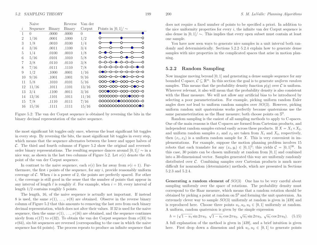
5.2. SAMPLING THEORY 199
Naive Reverse Van deri Sequence Binary Binary Corput Points in [0, 1]/ ∼1 0 .0000 .0000 02 1/16 .0001 .1000 1/23 1/8 .0010 .0100 1/44 3/16 .0011 .1100 3/45 1/4 .0100 .0010 1/86 5/16 .0101 .1010 5/87 3/8 .0110 .0110 3/88 7/16 .0111 .1110 7/89 1/2 .1000 .0001 1/1610 9/16 .1001 .1001 9/1611 5/8 .1010 .0101 5/1612 11/16 .1011 .1101 13/1613 3/4 .1100 .0011 3/1614 13/16 .1101 .1011 11/1615 7/8 .1110 .0111 7/1616 15/16 .1111 .1111 15/16
Figure 5.2: The van der Corput sequence is obtained by reversing the bits in thebinary decimal representation of the naive sequence.
the most significant bit toggles only once, whereas the least significant bit togglesin every step. By reversing the bits, the most significant bit toggles in every step,which means that the sequence alternates between the lower and upper halves ofC. The third and fourth columns of Figure 5.2 show the original and reversed-order binary representations. The resulting sequence dances around [0, 1]/ ∼ in anice way, as shown in the last two columns of Figure 5.2. Let ν(i) denote the ithpoint of the van der Corput sequence.
In contrast to the naive sequence, each ν(i) lies far away from ν(i + 1). Fur-thermore, the first i points of the sequence, for any i, provide reasonably uniformcoverage of C. When i is a power of 2, the points are perfectly spaced. For otheri, the coverage is still good in the sense that the number of points that appear inany interval of length l is roughly il. For example, when i = 10, every interval oflength 1/2 contains roughly 5 points.
The length, 16, of the naive sequence is actually not important. If instead8 is used, the same ν(1), . . ., ν(8) are obtained. Observe in the reverse binarycolumn of Figure 5.2 that this amounts to removing the last zero from each binarydecimal representation, which does not alter their values. If 32 is used for the naivesequence, then the same ν(1), . . ., ν(16) are obtained, and the sequence continuesnicely from ν(17) to ν(32). To obtain the van der Corput sequence from ν(33) toν(64), six-bit sequences are reversed (corresponding to the case in which the naivesequence has 64 points). The process repeats to produce an infinite sequence that
200 S. M. LaValle: Planning Algorithms
does not require a fixed number of points to be specified a priori. In addition tothe nice uniformity properties for every i, the infinite van der Corput sequence isalso dense in [0, 1]/ ∼. This implies that every open subset must contain at leastone sample.
You have now seen ways to generate nice samples in a unit interval both ran-domly and deterministically. Sections 5.2.2–5.2.4 explain how to generate densesamples with nice properties in the complicated spaces that arise in motion plan-ning.
5.2.2 Random Sampling
Now imagine moving beyond [0, 1] and generating a dense sample sequence for anybounded C-space, C ⊆ Rm. In this section the goal is to generate uniform randomsamples. This means that the probability density function p(q) over C is uniform.Wherever relevant, it also will mean that the probability density is also consistentwith the Haar measure. We will not allow any artificial bias to be introduced byselecting a poor parameterization. For example, picking uniform random Eulerangles does not lead to uniform random samples over SO(3). However, pickinguniform random unit quaternions works perfectly because quaternions use thesame parameterization as the Haar measure; both choose points on S3.
Random sampling is the easiest of all sampling methods to apply to C-spaces.One of the main reasons is that C-spaces are formed from Cartesian products, andindependent random samples extend easily across these products. If X = X1×X2,and uniform random samples x1 and x2 are taken from X1 and X2, respectively,then (x1, x2) is a uniform random sample for X. This is very convenient in im-plementations. For example, suppose the motion planning problem involves 15robots that each translate for any (xt, yt) ∈ [0, 1]2; this yields C = [0, 1]30. Inthis case, 30 points can be chosen uniformly at random from [0, 1] and combinedinto a 30-dimensional vector. Samples generated this way are uniformly randomlydistributed over C. Combining samples over Cartesian products is much moredifficult for nonrandom (deterministic) methods, which are presented in Sections5.2.3 and 5.2.4.
Generating a random element of SO(3) One has to be very careful aboutsampling uniformly over the space of rotations. The probability density mustcorrespond to the Haar measure, which means that a random rotation should beobtained by picking a point at random on S3 and forming the unit quaternion. Anextremely clever way to sample SO(3) uniformly at random is given in [439] andis reproduced here. Choose three points u1, u2, u3 ∈ [0, 1] uniformly at random.A uniform, random quaternion is given by the simple expression
h = (√1− u1 sin 2πu2,
√1− u1 cos 2πu2,
√u1 sin 2πu3,
√u1 cos 2πu3). (5.15)
A full explanation of the method is given in [439], and a brief intuition is givenhere. First drop down a dimension and pick u1, u2 ∈ [0, 1] to generate points

5.2. SAMPLING THEORY 201
on S2. Let u1 represent the value for the third coordinate, (0, 0, u1) ∈ R3. Theslice of points on S2 for which u1 is fixed for 0 < u1 < 1 yields a circle on S2
that corresponds to some line of latitude on S2. The second parameter selectsthe longitude, 2πu2. Fortunately, the points are uniformly distributed over S2.Why? Imagine S2 as the crust on a spherical loaf of bread that is run through abread slicer. The slices are cut in a direction parallel to the equator and are ofequal thickness. The crusts of each slice have equal area; therefore, the points areuniformly distributed. The method proceeds by using that fact that S3 can bepartitioned into a spherical arrangement of circles (known as the Hopf fibration);there is an S1 copy for each point in S2. The method above is used to providea random point on S2 using u2 and u3, and u1 produces a random point on S1;they are carefully combined in (5.15) to yield a random rotation. To respectthe antipodal identification for rotations, any quaternion h found in the lowerhemisphere (i.e., a < 0) can be negated to yield −h. This does not distort theuniform random distribution of the samples.
Generating random directions Some sampling-based algorithms require choos-ing motion directions at random.4 From a configuration q, the possible directionsof motion can be imagined as being distributed around a sphere. In an (n + 1)-dimensional C-space, this corresponds to sampling on Sn. For example, choosinga direction in R2 amounts to picking an element of S1; this can be parameter-ized as θ ∈ [0, 2π]/ ∼. If n = 4, then the previously mentioned trick for SO(3)should be used. If n = 3 or n > 4, then samples can be generated using a slightlymore expensive method that exploits spherical symmetries of the multidimensionalGaussian density function [176]. The method is explained for Rn+1; boundariesand identifications must be taken into account for other spaces. For each of then + 1 coordinates, generate a sample ui from a zero-mean Gaussian distributionwith the same variance for each coordinate. Following from the Central LimitTheorem, ui can be approximately obtained by generating k samples at randomover [−1, 1] and adding them (k ≥ 12 is usually sufficient in practice). The vector(u1, u2, . . . , un+1) gives a random direction in Rn+1 because each ui was obtainedindependently, and the level sets of the resulting probability density function arespheres. We did not use uniform random samples for each ui because this wouldbias the directions toward the corners of a cube; instead, the Gaussian yieldsspherical symmetry. The final step is to normalize the vector by taking ui/‖u‖for each coordinate.
Pseudorandom number generation Although there are advantages to uni-form random sampling, there are also several disadvantages. This motivates theconsideration of deterministic alternatives. Since there are trade-offs, it is impor-
4The directions will be formalized in Section 8.3.2 when smooth manifolds are introduced. Inthat case, the directions correspond to the set of possible velocities that have unit magnitude.Presently, the notion of a direction is only given informally.
202 S. M. LaValle: Planning Algorithms
tant to understand how to use both kinds of sampling in motion planning. Oneof the first issues is that computer-generated numbers are not random.5 A pseu-dorandom number generator is usually employed, which is a deterministic methodthat simulates the behavior of randomness. Since the samples are not truly ran-dom, the advantage of extending the samples over Cartesian products does notnecessarily hold. Sometimes problems are caused by unforeseen deterministic de-pendencies. One of the best pseudorandom number generators for avoiding suchtroubles is the Mersenne twister [355], for which implementations can be foundon the Internet.
To help see the general difficulties, the classical linear congruential pseudo-random number generator is briefly explained [317, 381]. The method uses threeinteger parameters, M , a, and c, which are chosen by the user. The first two,M and a, must be relatively prime, meaning that gcd(M,a) = 1. The third pa-rameter, c, must be chosen to satisfy 0 ≤ c < M . Using modular arithmetic, asequence can be generated as
yi+1 = ayi + c mod M, (5.16)
by starting with some arbitrary seed 1 ≤ y0 ≤ M . Pseudorandom numbers in[0, 1] are generated by the sequence
xi = yi/M. (5.17)
The sequence is periodic; therefore, M is typically very large (e.g., M = 231 − 1).Due to periodicity, there are potential problems of regularity appearing in thesamples, especially when applied across a Cartesian product to generate points inRn. Particular values must be chosen for the parameters, and statistical tests areused to evaluate the samples either experimentally or theoretically [381].
Testing for randomness Thus, it is important to realize that even the “ran-dom” samples are deterministic. They are designed to optimize performance onstatistical tests. Many sophisticated statistical tests of uniform randomness areused. One of the simplest, the chi-square test, is described here. This test mea-sures how far computed statistics are from their expected value. As a simpleexample, suppose C = [0, 1]2 and is partitioned into a 10 by 10 array of 100 squareboxes. If a set P of k samples is chosen at random, then intuitively each boxshould receive roughly k/100 of the samples. An error function can be defined tomeasure how far from true this intuition is:
e(P ) =100∑
i=1
(bi − k/100)2, (5.18)
in which bi is the number of samples that fall into box i. It is shown [269] thate(P ) follows a chi-squared distribution. A surprising fact is that the goal is not to
5There are exceptions, which use physical phenomena as a random source [407].

5.2. SAMPLING THEORY 203
minimize e(P ). If the error is too small, we would declare that the samples aretoo uniform to be random! Imagine k = 1, 000, 000 and exactly 10, 000 samplesappear in each of the 100 boxes. This yields e(P ) = 0, but how likely is this toever occur? The error must generally be larger (it appears in many statisticaltables) to account for the irregularity due to randomness.
(a) 196 pseudorandom samples (b) 196 pseudorandom samples
Figure 5.3: Irregularity in a collection of (pseudo)random samples can be nicelyobserved with Voronoi diagrams.
This irregularity can be observed in terms of Voronoi diagrams, as shown inFigure 5.3. The Voronoi diagram partitions R2 into regions based on the samples.Each sample x has an associated Voronoi region Vor(x). For any point y ∈Vor(x), x is the closest sample to y using Euclidean distance. The different sizesand shapes of these regions give some indication of the required irregularity ofrandom sampling. This irregularity may be undesirable for sampling-based motionplanning and is somewhat repaired by the deterministic sampling methods ofSections 5.2.3 and 5.2.4 (however, these methods also have drawbacks).
5.2.3 Low-Dispersion Sampling
This section describes an alternative to random sampling. Here, the goal is tooptimize a criterion called dispersion [381]. Intuitively, the idea is to place samplesin a way that makes the largest uncovered area be as small as possible. Thisgeneralizes of the idea of grid resolution. For a grid, the resolution may be selectedby defining the step size for each axis. As the step size is decreased, the resolutionincreases. If a grid-based motion planning algorithm can increase the resolutionarbitrarily, it becomes resolution complete. Using the concepts in this section,it may instead reduce its dispersion arbitrarily to obtain a resolution complete
204 S. M. LaValle: Planning Algorithms
(a) L2 dispersion (b) L∞ dispersion
Figure 5.4: Reducing the dispersion means reducing the radius of the largestempty ball.
algorithm. Thus, dispersion can be considered as a powerful generalization of thenotion of “resolution.”
Dispersion definition The dispersion6 of a finite set P of samples in a metricspace (X, ρ) is7
δ(P ) = supx∈X
minp∈P
ρ(x, p)
. (5.19)
Figure 5.4 gives an interpretation of the definition for two different metrics.An alternative way to consider dispersion is as the radius of the largest emptyball (for the L∞ metric, the balls are actually cubes). Note that at the boundaryof X (if it exists), the empty ball becomes truncated because it cannot exceedthe boundary. There is also a nice interpretation in terms of Voronoi diagrams.Figure 5.3 can be used to help explain L2 dispersion in R2. The Voronoi verticesare the points at which three or more Voronoi regions meet. These are points inC for which the nearest sample is far. An open, empty disc can be placed at anyVoronoi vertex, with a radius equal to the distance to the three (or more) closestsamples. The radius of the largest disc among those placed at all Voronoi verticesis the dispersion. This interpretation also extends nicely to higher dimensions.
Making good grids Optimizing dispersion forces the points to be distributedmore uniformly over C. This causes them to fail statistical tests, but the pointdistribution is often better for motion planning purposes. Consider the best wayto reduce dispersion if ρ is the L∞ metric and X = [0, 1]n. Suppose that thenumber of samples, k, is given. Optimal dispersion is obtained by partitioning
6The definition is unfortunately backward from intuition. Lower dispersion means that thepoints are nicely dispersed. Thus, more dispersion is bad, which is counterintuitive.
7The sup represents the supremum, which is the least upper bound. If X is closed, then thesup becomes a max. See Section 9.1.1 for more details.

5.2. SAMPLING THEORY 205
(a) 196-point Sukharev grid (b) 196 lattice points
Figure 5.5: The Sukharev grid and a nongrid lattice.
[0, 1] into a grid of cubes and placing a point at the center of each cube, as shownfor n = 2 and k = 196 in Figure 5.5a. The number of cubes per axis must be⌊k 1
n ⌋, in which ⌊·⌋ denotes the floor. If k 1n is not an integer, then there are leftover
points that may be placed anywhere without affecting the dispersion. Notice thatk
1n just gives the number of points per axis for a grid of k points in n dimensions.
The resulting grid will be referred to as a Sukharev grid [456].The dispersion obtained by the Sukharev grid is the best possible. Therefore,
a useful lower bound can be given for any set P of k samples [456]:
δ(P ) ≥ 1
2⌊
k1d
⌋ . (5.20)
This implies that keeping the dispersion fixed requires exponentially many pointsin the dimension, d.
At this point you might wonder why L∞ was used instead of L2, which seemsmore natural. This is because the L2 case is extremely difficult to optimize (exceptin R2, where a tiling of equilateral triangles can be made, with a point in the centerof each one). Even the simple problem of determining the best way to distributea fixed number of points in [0, 1]3 is unsolved for most values of k. See [131] forextensive treatment of this problem.
Suppose now that other topologies are considered instead of [0, 1]n. Let X =[0, 1]/ ∼, in which the identification produces a torus. The situation is quitedifferent because X no longer has a boundary. The Sukharev grid still producesoptimal dispersion, but it can also be shifted without increasing the dispersion.In this case, a standard grid may also be used, which has the same number ofpoints as the Sukharev grid but is translated to the origin. Thus, the first gridpoint is (0, 0), which is actually the same as 2n − 1 other points by identification.If X represents a cylinder and the number of points, k, is given, then it is best tojust use the Sukharev grid. It is possible, however, to shift each coordinate that
206 S. M. LaValle: Planning Algorithms
g1
g2
(a) (b)
Figure 5.6: (a) A distorted grid can even be placed over spheres and SO(3) byputting grids on the faces of an inscribed cube and lifting them to the surface[482]. (b) A lattice can be considered as a grid in which the generators are notnecessarily orthogonal.
behaves like S1. If X is rectangular but not a square, a good grid can still be madeby tiling the space with cubes. In some cases this will produce optimal dispersion.For complicated spaces such as SO(3), no grid exists in the sense defined so far.It is possible, however, to generate grids on the faces of an inscribed Platonic solid[139] and lift the samples to Sn with relatively little distortion [482]. For example,to sample S2, Sukharev grids can be placed on each face of a cube. These arelifted to obtain the warped grid shown in Figure 5.6a.
Example 5.15 (Sukharev Grid) Suppose that n = 2 and k = 9. IfX = [0, 1]2,then the Sukharev grid yields points for the nine cases in which either coordinatemay be 1/6, 1/2, or 5/6. The L∞ dispersion is 1/6. The spacing between the pointsalong each axis is 1/3, which is twice the dispersion. If instead X = [0, 1]2/ ∼,which represents a torus, then the nine points may be shifted to yield the stan-dard grid. In this case each coordinate may be 0, 1/3, or 2/3. The dispersion andspacing between the points remain unchanged.
One nice property of grids is that they have a lattice structure. This meansthat neighboring points can be obtained very easily be adding or subtractingvectors. Let gj be an n-dimensional vector called a generator. A point on a latticecan be expressed as
x =n∑
j=1
kjgj (5.21)
for n independent generators, as depicted in Figure 5.6b. In a 2D grid, the gen-erators represent “up” and “right.” If X = [0, 100]2 and a standard grid withinteger spacing is used, then the neighbors of the point (50, 50) are obtained byadding (0, 1), (0,−1), (−1, 0), or (1, 0). In a general lattice, the generators need

5.2. SAMPLING THEORY 207
not be orthogonal. An example is shown in Figure 5.5b. In Section 5.4.2, latticestructure will become important and convenient for defining the search graph.
Infinite grid sequences Now suppose that the number, k, of samples is notgiven. The task is to define an infinite sequence that has the nice properties ofthe van der Corput sequence but works for any dimension. This will become thenotion of a multi-resolution grid. The resolution can be iteratively doubled. For amulti-resolution standard grid in Rn, the sequence will first place one point at theorigin. After 2n points have been placed, there will be a grid with two points peraxis. After 4n points, there will be four points per axis. Thus, after 2ni points forany positive integer i, a grid with 2i points per axis will be represented. If onlycomplete grids are allowed, then it becomes clear why they appear inappropriatefor high-dimensional problems. For example, if n = 10, then full grids appearafter 1, 210, 220, 230, and so on, samples. Each doubling in resolution multipliesthe number of points by 2n. Thus, to use grids in high dimensions, one must bewilling to accept partial grids and define an infinite sequence that places points ina nice way.
The van der Corput sequence can be extended in a straightforward way asfollows. Suppose X = T2 = [0, 1]2/ ∼. The original van der Corput sequencestarted by counting in binary. The least significant bit was used to select whichhalf of [0, 1] was sampled. In the current setting, the two least significant bitscan be used to select the quadrant of [0, 1]2. The next two bits can be used toselect the quadrant within the quadrant. This procedure continues recursively toobtain a complete grid after k = 22i points, for any positive integer i. For anyk, however, there is only a partial grid. The points are distributed with optimalL∞ dispersion. This same idea can be applied in dimension n by using n bits ata time from the binary sequence to select the orthant (n-dimensional quadrant).Many other orderings produce L∞-optimal dispersion. Selecting orderings thatadditionally optimize other criteria, such as discrepancy or L2 dispersion, arecovered in [330, 335]. Unfortunately, it is more difficult to make a multi-resolutionSukharev grid. The base becomes 3 instead of 2; after every 3ni points a completegrid is obtained. For example, in one dimension, the first point appears at 1/2.The next two points appear at 1/6 and 5/6. The next complete one-dimensionalgrid appears after there are 9 points.
Dispersion bounds Since the sample sequence is infinite, it is interesting toconsider asymptotic bounds on dispersion. It is known that for X = [0, 1]n andany Lp metric, the best possible asymptotic dispersion is O(k−1/n) for k pointsand n dimensions [381]. In this expression, k is the variable in the limit and nis treated as a constant. Therefore, any function of n may appear as a constant(i.e., O(f(n)k−1/n) = O(k−1/n) for any positive f(n)). An important practicalconsideration is the size of f(n) in the asymptotic analysis. For example, for thevan der Corput sequence from Section 5.2.1, the dispersion is bounded by 1/k,
208 S. M. LaValle: Planning Algorithms
which means that f(n) = 1. This does not seem good because for values of kthat are powers of two, the dispersion is 1/2k. Using a multi-resolution Sukharevgrid, the constant becomes 3/2 because it takes a longer time before a full grid isobtained. Nongrid, low-dispersion infinite sequences exist that have f(n) = 1/ ln 4[381]; these are not even uniformly distributed, which is rather surprising.
5.2.4 Low-Discrepancy Sampling
In some applications, selecting points that align with the coordinate axis maybe undesirable. Therefore, extensive sampling theory has been developed to de-termine methods that avoid alignments while distributing the points uniformly.In sampling-based motion planning, grids sometimes yield unexpected behaviorbecause a row of points may align nicely with a corridor in Cfree. In some cases, asolution is obtained with surprisingly few samples, and in others, too many sam-ples are necessary. These alignment problems, when they exist, generally drive thevariance higher in computation times because it is difficult to predict when theywill help or hurt. This provides motivation for developing sampling techniquesthat try to reduce this sensitivity.
Discrepancy theory and its corresponding sampling methods were developed toavoid these problems for numerical integration [381]. Let X be a measure space,such as [0, 1]n. Let R be a collection of subsets of X that is called a range space.In most cases, R is chosen as the set of all axis-aligned rectangular subsets; hence,this will be assumed from this point onward. With respect to a particular pointset, P , and range space, R, the discrepancy [472] for k samples is defined as (seeFigure 5.7)
D(P,R) = supR∈R
∣
∣
∣
∣
|P ∩R|k
− µ(R)
µ(X)
∣
∣
∣
∣
, (5.22)
in which |P ∩ R| denotes the number of points in P ∩ R. Each term in thesupremum considers how well P can be used to estimate the volume of R. Forexample, if µ(R) is 1/5, then we would hope that about 1/5 of the points in Pfall into R. The discrepancy measures the largest volume estimation error thatcan be obtained over all sets in R.
Asymptotic bounds There are many different asymptotic bounds for discrep-ancy, depending on the particular range space and measure space [353]. The mostwidely referenced bounds are based on the standard range space of axis-alignedrectangular boxes in [0, 1]n. There are two different bounds, depending on whetherthe number of points, k, is given. The best possible asymptotic discrepancy for asingle sequence is O(k−1 logn k). This implies that k is not specified. If, however,for every k a new set of points can be chosen, then the best possible discrepancyis O(k−1 logn−1 k). This bound is lower because it considers the best that can beachieved by a sequence of points sets, in which every point set may be completely

5.2. SAMPLING THEORY 209
R
Figure 5.7: Discrepancy measures whether the right number of points fall intoboxes. It is related to the chi-square test but optimizes over all possible boxes.
different. In a single sequence, the next set must be extended from the currentset by adding a single sample.
Relating dispersion and discrepancy Since balls have positive volume, thereis a close relationship between discrepancy, which is measure-based, and disper-sion, which is metric-based. For example, for any P ⊂ [0, 1]n,
δ(P,L∞) ≤ D(P,R)1/d, (5.23)
which means low-discrepancy implies low-dispersion. Note that the converse isnot true. An axis-aligned grid yields high discrepancy because of alignments withthe boundaries of sets in R, but the dispersion is very low. Even though low-discrepancy implies low-dispersion, lower dispersion can usually be obtained byignoring discrepancy (this is one less constraint to worry about). Thus, a trade-offmust be carefully considered in applications.
Low-discrepancy sampling methods Due to the fundamental importance ofnumerical integration and the intricate link between discrepancy and integrationerror, most sampling literature has led to low-discrepancy sequences and point sets[381, 443, 458]. Although motion planning is quite different from integration, itis worth evaluating these carefully constructed and well-analyzed samples. Theirpotential use in motion planning is no less reasonable than using pseudorandomsequences, which were also designed with a different intention in mind (satisfyingstatistical tests of randomness).
Low-discrepancy sampling methods can be divided into three categories: 1)Halton/Hammersley sampling; 2) (t,s)-sequences and (t,m,s)-nets; and 3) lattices.The first category represents one of the earliest methods, and is based on extendingthe van der Corput sequence. The Halton sequence is an n-dimensional generaliza-tion of the van der Corput sequence, but instead of using binary representations,
210 S. M. LaValle: Planning Algorithms
a different basis is used for each coordinate [220]. The result is a reasonable de-terministic replacement for random samples in many applications. The resultingdiscrepancy (and dispersion) is lower than that for random samples (with highprobability). Figure 5.8a shows the first 196 Halton points in R2.
Choose n relatively prime integers p1, p2, . . . , pn (usually the first n primes,p1 = 2, p2 = 3, . . ., are chosen). To construct the ith sample, consider the base-prepresentation for i, which takes the form i = a0 + pa1 + p2a2 + p3a3 + . . .. Thefollowing point in [0, 1] is obtained by reversing the order of the bits and movingthe decimal point (as was done in Figure 5.2):
r(i, p) =a0p
+a1p2
+a2p3
+a3p4
+ · · · . (5.24)
For p = 2, this yields the ith point in the van der Corput sequence. Starting fromi = 0, the ith sample in the Halton sequence is
(
r(i, p1), r(i, p2), . . . , r(i, pn))
. (5.25)
Suppose instead that k, the required number of points, is known. In this case,a better distribution of samples can be obtained. The Hammersley point set [221]is an adaptation of the Halton sequence. Using only d − 1 distinct primes andstarting at i = 0, the ith sample in a Hammersley point set with k elements is
(
i/k, r(i, p1), . . . , r(i, pn−1))
. (5.26)
Figure 5.8b shows the Hammersley set for n = 2 and k = 196.The construction of Halton/Hammersley samples is simple and efficient, which
has led to widespread application. They both achieve asymptotically optimaldiscrepancy; however, the constant in their asymptotic analysis increases morethan exponentially with dimension [381]. The constant for the dispersion alsoincreases exponentially, which is much worse than for the methods of Section5.2.3.
Improved constants are obtained for sequences and finite points by using (t,s)-sequences, and (t,m,s)-nets, respectively [381]. The key idea is to enforce zerodiscrepancy over particular subsets of R known as canonical rectangles, and allremaining ranges in R will contribute small amounts to discrepancy. The mostfamous and widely used (t,s)-sequences are Sobol’ and Faure (see [381]). TheNiederreiter-Xing (t,s)-sequence has the best-known asymptotic constant, (a/n)n,in which a is a small positive constant [382].
The third category is lattices, which can be considered as a generalization ofgrids that allows nonorthogonal axes [353, 443, 469]. As an example, considerFigure 5.5b, which shows 196 lattice points generated by the following technique.Let α be a positive irrational number. For a fixed k, generate the ith pointaccording to (i/k, iα), in which · denotes the fractional part of the real value(modulo-one arithmetic). In Figure 5.5b, α = (
√5 + 1)/2, the golden ratio.
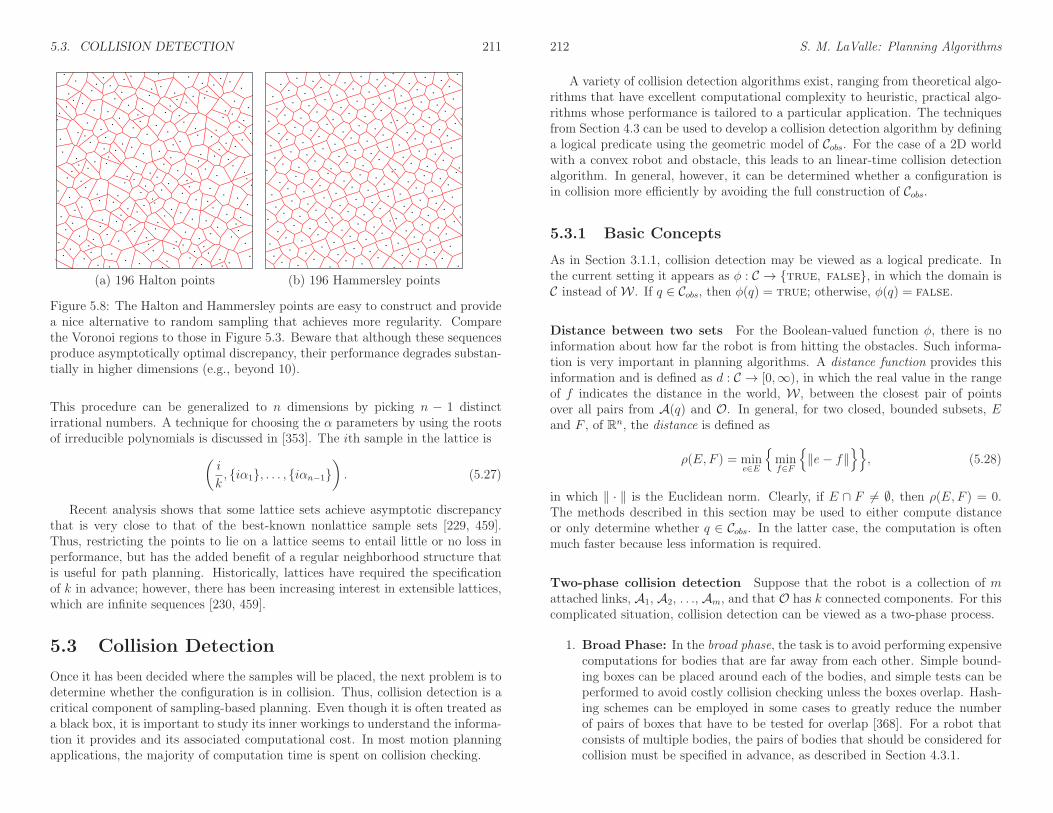
5.3. COLLISION DETECTION 211
(a) 196 Halton points (b) 196 Hammersley points
Figure 5.8: The Halton and Hammersley points are easy to construct and providea nice alternative to random sampling that achieves more regularity. Comparethe Voronoi regions to those in Figure 5.3. Beware that although these sequencesproduce asymptotically optimal discrepancy, their performance degrades substan-tially in higher dimensions (e.g., beyond 10).
This procedure can be generalized to n dimensions by picking n − 1 distinctirrational numbers. A technique for choosing the α parameters by using the rootsof irreducible polynomials is discussed in [353]. The ith sample in the lattice is
(
i
k, iα1, . . . , iαn−1
)
. (5.27)
Recent analysis shows that some lattice sets achieve asymptotic discrepancythat is very close to that of the best-known nonlattice sample sets [229, 459].Thus, restricting the points to lie on a lattice seems to entail little or no loss inperformance, but has the added benefit of a regular neighborhood structure thatis useful for path planning. Historically, lattices have required the specificationof k in advance; however, there has been increasing interest in extensible lattices,which are infinite sequences [230, 459].
5.3 Collision Detection
Once it has been decided where the samples will be placed, the next problem is todetermine whether the configuration is in collision. Thus, collision detection is acritical component of sampling-based planning. Even though it is often treated asa black box, it is important to study its inner workings to understand the informa-tion it provides and its associated computational cost. In most motion planningapplications, the majority of computation time is spent on collision checking.
212 S. M. LaValle: Planning Algorithms
A variety of collision detection algorithms exist, ranging from theoretical algo-rithms that have excellent computational complexity to heuristic, practical algo-rithms whose performance is tailored to a particular application. The techniquesfrom Section 4.3 can be used to develop a collision detection algorithm by defininga logical predicate using the geometric model of Cobs. For the case of a 2D worldwith a convex robot and obstacle, this leads to an linear-time collision detectionalgorithm. In general, however, it can be determined whether a configuration isin collision more efficiently by avoiding the full construction of Cobs.
5.3.1 Basic Concepts
As in Section 3.1.1, collision detection may be viewed as a logical predicate. Inthe current setting it appears as φ : C → true, false, in which the domain isC instead of W . If q ∈ Cobs, then φ(q) = true; otherwise, φ(q) = false.
Distance between two sets For the Boolean-valued function φ, there is noinformation about how far the robot is from hitting the obstacles. Such informa-tion is very important in planning algorithms. A distance function provides thisinformation and is defined as d : C → [0,∞), in which the real value in the rangeof f indicates the distance in the world, W , between the closest pair of pointsover all pairs from A(q) and O. In general, for two closed, bounded subsets, Eand F , of Rn, the distance is defined as
ρ(E,F ) = mine∈E
minf∈F
‖e− f‖
, (5.28)
in which ‖ · ‖ is the Euclidean norm. Clearly, if E ∩ F 6= ∅, then ρ(E,F ) = 0.The methods described in this section may be used to either compute distanceor only determine whether q ∈ Cobs. In the latter case, the computation is oftenmuch faster because less information is required.
Two-phase collision detection Suppose that the robot is a collection of mattached links, A1, A2, . . ., Am, and that O has k connected components. For thiscomplicated situation, collision detection can be viewed as a two-phase process.
1. Broad Phase: In the broad phase, the task is to avoid performing expensivecomputations for bodies that are far away from each other. Simple bound-ing boxes can be placed around each of the bodies, and simple tests can beperformed to avoid costly collision checking unless the boxes overlap. Hash-ing schemes can be employed in some cases to greatly reduce the numberof pairs of boxes that have to be tested for overlap [368]. For a robot thatconsists of multiple bodies, the pairs of bodies that should be considered forcollision must be specified in advance, as described in Section 4.3.1.

5.3. COLLISION DETECTION 213
(a) (b) (c) (d)
Figure 5.9: Four different kinds of bounding regions: (a) sphere, (b) axis-alignedbounding box (AABB), (c) oriented bounding box (OBB), and (d) convex hull.Each usually provides a tighter approximation than the previous one but is moreexpensive to test for overlapping pairs.
2. Narrow Phase: In the narrow phase, individual pairs of bodies are eachchecked carefully for collision. Approaches to this phase are described inSections 5.3.2 and 5.3.3.
5.3.2 Hierarchical Methods
In this section, suppose that two complicated, nonconvex bodies, E and F , areto be checked for collision. Each body could be part of either the robot or theobstacle region. They are subsets of R2 or R3, defined using any kind of geometricprimitives, such as triangles in R3. Hierarchical methods generally decomposeeach body into a tree. Each vertex in the tree represents a bounding region thatcontains some subset of the body. The bounding region of the root vertex containsthe whole body.
There are generally two opposing criteria that guide the selection of the typeof bounding region:
1. The region should fit the intended body points as tightly as possible.
2. The intersection test for two regions should be as efficient as possible.
Several popular choices are shown in Figure 5.9 for an L-shaped body.The tree is constructed for a body, E (or alternatively, F ) recursively as fol-
lows. For each vertex, consider the set X of all points in E that are contained inthe bounding region. Two child vertices are constructed by defining two smallerbounding regions whose union covers X. The split is made so that the portioncovered by each child is of similar size. If the geometric model consists of primi-tives such as triangles, then a split could be made to separate the triangles intotwo sets of roughly the same number of triangles. A bounding region is thencomputed for each of the children. Figure 5.10 shows an example of a split for thecase of an L-shaped body. Children are generated recursively by making splitsuntil very simple sets are obtained. For example, in the case of triangles in space,
214 S. M. LaValle: Planning Algorithms
Figure 5.10: The large circle shows the bounding region for a vertex that coversan L-shaped body. After performing a split along the dashed line, two smallercircles are used to cover the two halves of the body. Each circle corresponds to achild vertex.
a split is made unless the vertex represents a single triangle. In this case, it iseasy to test for the intersection of two triangles.
Consider the problem of determining whether bodies E and F are in collision.Suppose that the trees Te and Tf have been constructed for E and F , respectively.If the bounding regions of the root vertices of Te and Tf do not intersect, then itis known that Te and Tf are not in collision without performing any additionalcomputation. If the bounding regions do intersect, then the bounding regions ofthe children of Te are compared to the bounding region of Tf . If either of theseintersect, then the bounding region of Tf is replaced with the bounding regionsof its children, and the process continues recursively. As long as the boundingregions overlap, lower levels of the trees are traversed, until eventually the leavesare reached. If triangle primitives are used for the geometric models, then at theleaves the algorithm tests the individual triangles for collision, instead of boundingregions. Note that as the trees are traversed, if a bounding region from the vertexv1 of Te does not intersect the bounding region from a vertex, v2, of Tf , then nochildren of v1 have to be compared to children of v1. Usually, this dramaticallyreduces the number of comparisons, relative in a naive approach that tests allpairs of triangles for intersection.
It is possible to extend the hierarchical collision detection scheme to also com-pute distance. The closest pair of points found so far serves as an upper boundthat prunes aways some future pairs from consideration. If a pair of boundingregions has a distance greater than the smallest distance computed so far, thentheir children do not have to be considered [329]. In this case, an additional re-quirement usually must be imposed. Every bounding region must be a propersubset of its parent bounding region [406]. If distance information is not needed,then this requirement can be dropped.
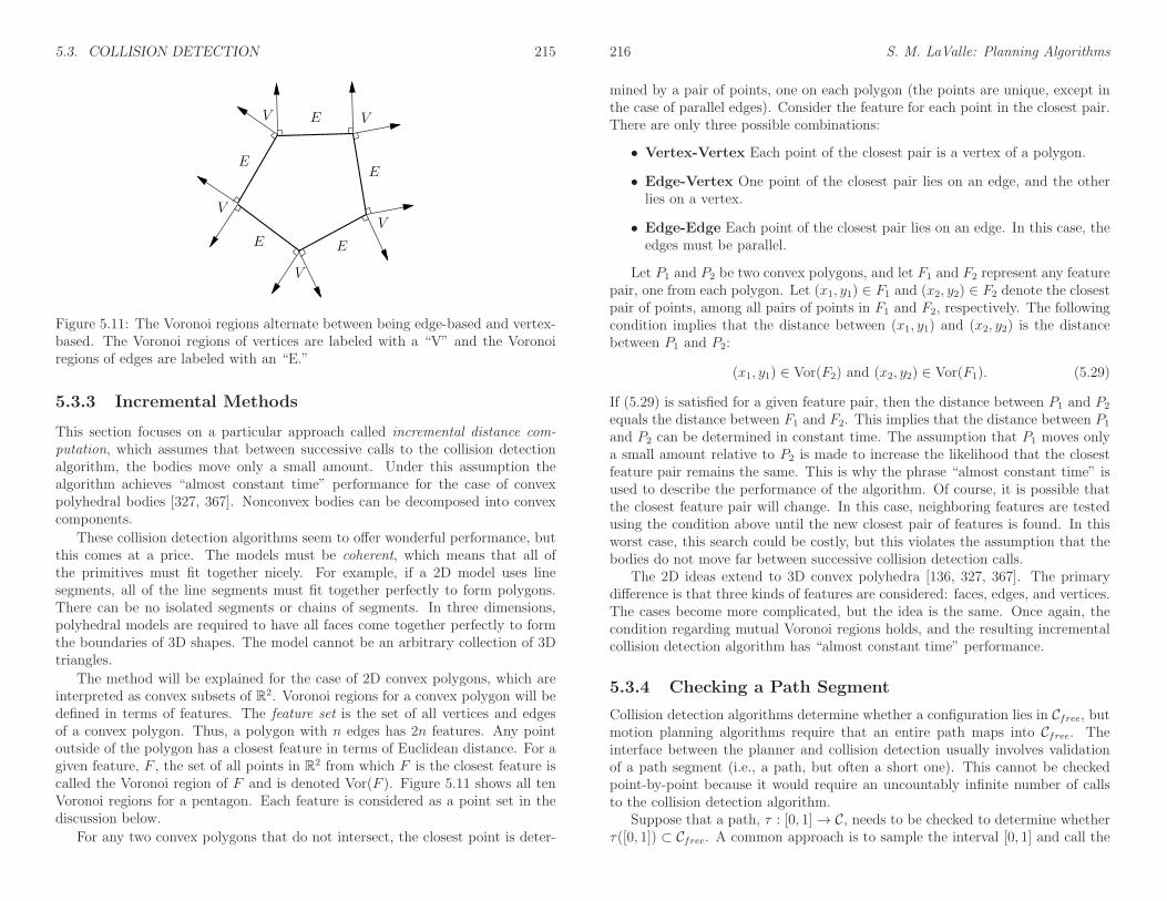
5.3. COLLISION DETECTION 215
V
V
V
E
E
E
V
E
E
V
Figure 5.11: The Voronoi regions alternate between being edge-based and vertex-based. The Voronoi regions of vertices are labeled with a “V” and the Voronoiregions of edges are labeled with an “E.”
5.3.3 Incremental Methods
This section focuses on a particular approach called incremental distance com-putation, which assumes that between successive calls to the collision detectionalgorithm, the bodies move only a small amount. Under this assumption thealgorithm achieves “almost constant time” performance for the case of convexpolyhedral bodies [327, 367]. Nonconvex bodies can be decomposed into convexcomponents.
These collision detection algorithms seem to offer wonderful performance, butthis comes at a price. The models must be coherent, which means that all ofthe primitives must fit together nicely. For example, if a 2D model uses linesegments, all of the line segments must fit together perfectly to form polygons.There can be no isolated segments or chains of segments. In three dimensions,polyhedral models are required to have all faces come together perfectly to formthe boundaries of 3D shapes. The model cannot be an arbitrary collection of 3Dtriangles.
The method will be explained for the case of 2D convex polygons, which areinterpreted as convex subsets of R2. Voronoi regions for a convex polygon will bedefined in terms of features. The feature set is the set of all vertices and edgesof a convex polygon. Thus, a polygon with n edges has 2n features. Any pointoutside of the polygon has a closest feature in terms of Euclidean distance. For agiven feature, F , the set of all points in R2 from which F is the closest feature iscalled the Voronoi region of F and is denoted Vor(F ). Figure 5.11 shows all tenVoronoi regions for a pentagon. Each feature is considered as a point set in thediscussion below.
For any two convex polygons that do not intersect, the closest point is deter-
216 S. M. LaValle: Planning Algorithms
mined by a pair of points, one on each polygon (the points are unique, except inthe case of parallel edges). Consider the feature for each point in the closest pair.There are only three possible combinations:
• Vertex-Vertex Each point of the closest pair is a vertex of a polygon.
• Edge-Vertex One point of the closest pair lies on an edge, and the otherlies on a vertex.
• Edge-Edge Each point of the closest pair lies on an edge. In this case, theedges must be parallel.
Let P1 and P2 be two convex polygons, and let F1 and F2 represent any featurepair, one from each polygon. Let (x1, y1) ∈ F1 and (x2, y2) ∈ F2 denote the closestpair of points, among all pairs of points in F1 and F2, respectively. The followingcondition implies that the distance between (x1, y1) and (x2, y2) is the distancebetween P1 and P2:
(x1, y1) ∈ Vor(F2) and (x2, y2) ∈ Vor(F1). (5.29)
If (5.29) is satisfied for a given feature pair, then the distance between P1 and P2
equals the distance between F1 and F2. This implies that the distance between P1
and P2 can be determined in constant time. The assumption that P1 moves onlya small amount relative to P2 is made to increase the likelihood that the closestfeature pair remains the same. This is why the phrase “almost constant time” isused to describe the performance of the algorithm. Of course, it is possible thatthe closest feature pair will change. In this case, neighboring features are testedusing the condition above until the new closest pair of features is found. In thisworst case, this search could be costly, but this violates the assumption that thebodies do not move far between successive collision detection calls.
The 2D ideas extend to 3D convex polyhedra [136, 327, 367]. The primarydifference is that three kinds of features are considered: faces, edges, and vertices.The cases become more complicated, but the idea is the same. Once again, thecondition regarding mutual Voronoi regions holds, and the resulting incrementalcollision detection algorithm has “almost constant time” performance.
5.3.4 Checking a Path Segment
Collision detection algorithms determine whether a configuration lies in Cfree, butmotion planning algorithms require that an entire path maps into Cfree. Theinterface between the planner and collision detection usually involves validationof a path segment (i.e., a path, but often a short one). This cannot be checkedpoint-by-point because it would require an uncountably infinite number of callsto the collision detection algorithm.
Suppose that a path, τ : [0, 1]→ C, needs to be checked to determine whetherτ([0, 1]) ⊂ Cfree. A common approach is to sample the interval [0, 1] and call the

5.3. COLLISION DETECTION 217
A x
y
ar
r
Figure 5.12: The furthest point on A from the origin travels the fastest when Ais rotated. At most it can be displaced by 2πr, if xt and yt are fixed.
collision checker only on the samples. What resolution of sampling is required?How can one ever guarantee that the places where the path is not sampled arecollision-free? There are both practical and theoretical answers to these questions.In practice, a fixed ∆q > 0 is often chosen as the C-space step size. Points t1, t2 ∈[0, 1] are then chosen close enough together to ensure that ρ(τ(t1), τ(t2)) ≤ ∆q, inwhich ρ is the metric on C. The value of ∆q is often determined experimentally.If ∆q is too small, then considerable time is wasted on collision checking. If ∆qis too large, then there is a chance that the robot could jump through a thinobstacle.
Setting ∆q empirically might not seem satisfying. Fortunately, there are soundalgorithmic ways to verify that a path is collision-free. In some applications themethods are still not used because they are trickier to implement and they oftenyield worse performance. Therefore, both methods are presented here, and youcan decide which is appropriate, depending on the context and your personaltastes.
Ensuring that τ([0, 1]) ⊂ Cfree requires the use of both distance informationand bounds on the distance that points on A can travel in R. Such bounds canbe obtained by using the robot displacement metric from Example 5.6. Beforeexpressing the general case, first we will explain the concept in terms of a rigidrobot that translates and rotates in W = R2. Let xt, yt ∈ R2 and θ ∈ [0, 2π]/ ∼.Suppose that a collision detection algorithm indicates that A(q) is at least dunits away from collision with obstacles in W . This information can be used todetermine a region in Cfree that contains q. Suppose that the next candidateconfiguration to be checked along τ is q′. If no point on A travels more thandistance d when moving from q to q′ along τ , then q′ and all configurations betweenq and q′ must be collision-free. This assumes that on the path from q to q′, everyvisited configuration must lie between qi and q
′i for the ith coordinate and any i
from 1 to n. If the robot can instead take any path between q and q′, then nosuch guarantee can be made).
218 S. M. LaValle: Planning Algorithms
When A undergoes a translation, all points move the same distance. Forrotation, however, the distance traveled depends on how far the point on A isfrom the rotation center, (0, 0). Let ar = (xr, yr) denote the point on A thathas the largest magnitude, r =
√
x2r + y2r . Figure 5.12 shows an example. Atransformed point a ∈ A may be denoted by a(xt, yt, θ). The following bound isobtained for any a ∈ A, if the robot is rotated from orientation θ to θ′:
‖a(xt, yt, θ)− a(xt, yt, θ′)‖ ≤ ‖ar(xt, yt, θ)− ar(xt, yt, θ′)‖ < r|θ − θ′|, (5.30)
assuming that a path in C is followed that interpolates between θ and θ′ (usingthe shortest path in S1 between θ and θ′). Thus, if A(q) is at least d away fromthe obstacles, then the orientation may be changed without causing collision aslong as r|θ − θ′| < d. Note that this is a loose upper bound because ar travelsalong a circular arc and can be displaced by no more than 2πr.
Similarly, xt and yt may individually vary up to d, yielding |xt − x′t| < d and|yt − y′t| < d. If all three parameters vary simultaneously, then a region in Cfreecan be defined as
(x′t, y′t, θ′) ∈ C | |xt − x′t|+ |yt − y′t|+ r|θ − θ′| < d. (5.31)
Such bounds can generally be used to set a step size, ∆q, for collision checkingthat guarantees the intermediate points lie in Cfree. The particular value usedmay vary depending on d and the direction8 of the path.
For the case of SO(3), once again the displacement of the point on A thathas the largest magnitude can be bounded. It is best in this case to express thebounds in terms of quaternion differences, ‖h−h′‖. Euler angles may also be usedto obtain a straightforward generalization of (5.31) that has six terms, three fortranslation and three for rotation. For each of the three rotation parts, a pointwith the largest magnitude in the plane perpendicular to the rotation axis mustbe chosen.
If there are multiple links, it becomes much more complicated to determine thestep size. Each point a ∈ Ai is transformed by some nonlinear function based onthe kinematic expressions from Sections 3.3 and 3.4. Let a : C → W denote thistransformation. In some cases, it might be possible to derive a Lipschitz conditionof the form
‖a(q)− a(q′)‖ < c‖q − q′‖, (5.32)
in which c ∈ (0,∞) is a fixed constant, a is any point on Ai, and the expressionholds for any q, q′ ∈ C. The goal is to make the Lipschitz constant, c, as small aspossible; this enables larger variations in q.
A better method is to individually bound the link displacement with respectto each parameter,
‖a(q1, . . . , qi−1, qi, qi+1, . . . , qn)− a(q1, . . . , qi−1, q′i, qi+1, . . . , qn)‖ < ci|qi − q′i|,
(5.33)
8To formally talk about directions, it would be better to define a differentiable structure onC. This will be deferred to Section 8.3, where it seems unavoidable.
5.4. INCREMENTAL SAMPLING AND SEARCHING 219
to obtain the Lipschitz constants c1, . . ., cn. The bound on robot displacementbecomes
‖a(q)− a(q′)‖ <n∑
i=1
ci|qi − q′i|. (5.34)
The benefit of using individual parameter bounds can be seen by considering a longchain. Consider a 50-link chain of line segments in R2, and each link has length10. The C-space is T50, which can be parameterized as [0, 2π]50/ ∼. Suppose thatthe chain is in a straight-line configuration (θi = 0 for all 1 ≤ i ≤ 50), whichmeans that the last point is at (500, 0) ∈ W . Changes in θ1, the orientation ofthe first link, dramatically move A50. However, changes in θ50 move A50 a smalleramount. Therefore, it is advantageous to pick a different ∆qi for each 1 ≤ i ≤ 50.In this example, a smaller value should be used for ∆θ1 in comparison to ∆θ50.
Unfortunately, there are more complications. Suppose the 50-link chain isin a configuration that folds all of the links on top of each other (θi = π foreach 1 ≤ i ≤ n). In this case, A50 does not move as fast when θ1 is perturbed,in comparison to the straight-line configuration. A larger step size for θ1 couldbe used for this configuration, relative to other parts of C. The implication isthat, although Lipschitz constants can be made to hold over all of C, it might bepreferable to determine a better bound in a local region around q ∈ C. A linearmethod could be obtained by analyzing the Jacobian of the transformations, suchas (3.53) and (3.57).
Another important concern when checking a path is the order in which thesamples are checked. For simplicity, suppose that ∆q is constant and that the pathis a constant-speed parameterization. Should the collision checker step along from0 up to 1? Experimental evidence indicates that it is best to use a recursive binarystrategy [191]. This makes no difference if the path is collision-free, but it oftensaves time if the path is in collision. This is a kind of sampling problem over[0, 1], which is addressed nicely by the van der Corput sequence, ν. The lastcolumn in Figure 5.2 indicates precisely where to check along the path in eachstep. Initially, τ(1) is checked. Following this, points from the van der Corputsequence are checked in order: τ(0), τ(1/2), τ(1/4), τ(3/4), τ(1/8), . . .. Theprocess terminates if a collision is found or when the dispersion falls below ∆q.If ∆q is not constant, then it is possible to skip over some points of ν in regionswhere the allowable variation in q is larger.
5.4 Incremental Sampling and Searching
5.4.1 The General Framework
The algorithms of Sections 5.4 and 5.5 follow the single-query model, which means(qI , qG) is given only once per robot and obstacle set. This means that there are noadvantages to precomputation, and the sampling-based motion planning problem
220 S. M. LaValle: Planning Algorithms
can be considered as a kind of search. The multiple-query model, which favorsprecomputation, is covered in Section 5.6.
The sampling-based planning algorithms presented in the present section arestrikingly similar to the family of search algorithms summarized in Section 2.2.4.The main difference lies in step 3 below, in which applying an action, u, is replacedby generating a path segment, τs. Another difference is that the search graph, G,is undirected, with edges that represent paths, as opposed to a directed graph inwhich edges represent actions. It is possible to make these look similar by definingan action space for motion planning that consists of a collection of paths, but thisis avoided here. In the case of motion planning with differential constraints, thiswill actually be required; see Chapter 14.
Most single-query, sampling-based planning algorithms follow this template:
1. Initialization: Let G(V,E) represent an undirected search graph, for whichV contains at least one vertex and E contains no edges. Typically, V con-tains qI , qG, or both. In general, other points in Cfree may be included.
2. Vertex Selection Method (VSM): Choose a vertex qcur ∈ V for expan-sion.
3. Local Planning Method (LPM): For some qnew ∈ Cfree that may ormay not be represented by a vertex in V , attempt to construct a pathτs : [0, 1]→ Cfree such that τ(0) = qcur and τ(1) = qnew. Using the methodsof Section 5.3.4, τs must be checked to ensure that it does not cause acollision. If this step fails to produce a collision-free path segment, then goto step 2.
4. Insert an Edge in the Graph: Insert τs into E, as an edge from qcur toqnew. If qnew is not already in V , then it is inserted.
5. Check for a Solution: Determine whether G encodes a solution path.As in the discrete case, if there is a single search tree, then this is trivial;otherwise, it can become complicated and expensive.
6. Return to Step 2: Iterate unless a solution has been found or some ter-mination condition is satisfied, in which case the algorithm reports failure.
In the present context, G is a topological graph, as defined in Example 4.6.Each vertex is a configuration and each edge is a path that connects two configu-rations. In this chapter, it will be simply referred to as a graph when there is nochance of confusion. Some authors refer to such a graph as a roadmap; however,we reserve the term roadmap for a graph that contains enough paths to make anymotion planning query easily solvable. This case is covered in Section 5.6 andthroughout Chapter 6.
A large family of sampling-based algorithms can be described by varying theimplementations of steps 2 and 3. Implementations of the other steps may also

5.4. INCREMENTAL SAMPLING AND SEARCHING 221
qI qG
qI qG
(a) (b)
qGqI
qGqI
(c) (d)
Figure 5.13: All of these depict high-dimensional obstacle regions in C-space. (a)The search must involve some sort of multi-resolution aspect, otherwise, that al-gorithm may explore too many points within a cavity. (b) Sometimes the problemis like a bug trap, in which case bidirectional search can help. (c) For a doublebug trap, multi-directional search may be needed. (d) This example is hard tosolve even for multi-directional search.
vary, but this is less important and will be described where appropriate. Forconvenience, step 2 will be called the vertex selection method (VSM) and step 3will be called the local planning method (LPM). The role of the VSM is similar tothat of the priority queue, Q, in Section 2.2.1. The role of the LPM is to computea collision-free path segment that can be added to the graph. It is called localbecause the path segment is usually simple (e.g., the shortest path) and travels ashort distance. It is not global in the sense that the LPM does not try to solve theentire planning problem; it is expected that the LPM may often fail to constructpath segments.
It will be formalized shortly, but imagine for the time being that any of thesearch algorithms from Section 2.2 may be applied to motion planning by ap-proximating C with a high-resolution grid. The resulting problem looks like amulti-dimensional extension of Example 2.1 (the “labyrinth” walls are formedby Cobs). For a high-resolution grid in a high-dimensional space, most classicaldiscrete searching algorithms have trouble getting trapped in a local minimum.There could be an astronomical number of configurations that fall within a con-
222 S. M. LaValle: Planning Algorithms
cavity in Cobs that must be escaped to solve the problem, as shown in Figure5.13a. Imagine a problem in which the C-space obstacle is a giant “bowl” thatcan trap the configuration. This figure is drawn in two dimensions, but imaginethat the C has many dimensions, such as six for SE(3) or perhaps dozens for alinkage. If the discrete planning algorithms from Section 2.2 are applied to a high-resolution grid approximation of C, then they will all waste their time filling upthe bowl before being able to escape to qG. The number of grid points in this bowlwould typically be on the order of 100n for an n-dimensional C-space. Therefore,sampling-based motion planning algorithms combine sampling and searching in away that attempts to overcome this difficulty.
As in the case of discrete search algorithms, there are several classes of algo-rithms based on the number of search trees.
Unidirectional (single-tree) methods: In this case, the planning ap-pears very similar to discrete forward search, which was given in Figure 2.4.The main difference between algorithms in this category is how they imple-ment the VSM and LPM. Figure 5.13b shows a bug trap9 example for whichforward-search algorithms would have great trouble; however, the problemmight not be difficult for backward search, if the planner incorporates somekind of greedy, best-first behavior. This example, again in high dimensions,can be considered as a kind of “bug trap.” To leave the trap, a path mustbe found from qI into the narrow opening. Imagine a fly buzzing aroundthrough the high-dimensional trap. The escape opening might not look toodifficult in two dimensions, but if it has a small range with respect to eachconfiguration parameter, it is nearly impossible to find the opening. The tipof the “volcano” would be astronomically small compared to the rest of thebug trap. Examples such as this provide some motivation for bidirectionalalgorithms. It might be easier for a search tree that starts in qG to arrive inthe bug trap.
Bidirectional (two-tree) methods: Since it is not known whether qI orqG might lie in a bug trap (or another challenging region), a bidirectionalapproach is often preferable. This follows from an intuition that two prop-agating wavefronts, one centered on qI and the other on qG, will meet aftercovering less area in comparison to a single wavefront centered at qI thatmust arrive at qG. A bidirectional search is achieved by defining the VSMto alternate between trees when selecting vertices. The LPM sometimesgenerates paths that explore new parts of Cfree, and at other times it triesto generate a path that connects the two trees.
Multi-directional (more than two trees) methods: If the problemis so bad that a double bug trap exists, as shown in Figure 5.13c, then it
9This principle is actually used in real life to trap flying bugs. This analogy was suggestedby James O’Brien in a discussion with James Kuffner.

5.4. INCREMENTAL SAMPLING AND SEARCHING 223
might make sense to grow trees from other places in the hopes that there arebetter chances to enter the traps in the other direction. This complicatesthe problem of connecting trees, however. Which pairs of trees should beselected in each iteration for possible connection? How often should the samepair be selected? Which vertex pairs should be selected? Many heuristicparameters may arise in practice to answer these questions.
Of course, one can play the devil’s advocate and construct the example in Figure5.13d, for which virtually all sampling-based planning algorithms are doomed.Even harder versions can be made in which a sequence of several narrow corridorsmust be located and traversed. We must accept the fact that some problems arehopeless to solve using sampling-based planning methods, unless there is someproblem-specific structure that can be additionally exploited.
5.4.2 Adapting Discrete Search Algorithms
One of the most convenient and straightforward ways to make sampling-basedplanning algorithms is to define a grid over C and conduct a discrete search usingthe algorithms of Section 2.2. The resulting planning problem actually looks verysimilar to Example 2.1. Each edge now corresponds to a path in Cfree. Some edgesmay not exist because of collisions, but this will have to be revealed incrementallyduring the search because an explicit representation of Cobs is too expensive toconstruct (recall Section 4.3).
Assume that an n-dimensional C-space is represented as a unit cube, C =[0, 1]n/ ∼, in which ∼ indicates that identifications of the sides of the cube aremade to reflect the C-space topology. Representing C as a unit cube usuallyrequires a reparameterization. For example, an angle θ ∈ [0, 2π) would be replacedwith θ/2π to make the range lie within [0, 1]. If quaternions are used for SO(3),then the upper half of S3 must be deformed into [0, 1]3/ ∼.
Discretization Assume that C is discretized by using the resolutions k1, k2,. . .,and kn, in which each ki is a positive integer. This allows the resolution to bedifferent for each C-space coordinate. Either a standard grid or a Sukharev gridcan be used. Let
∆qi = [0 · · · 0 1/ki 0 · · · 0], (5.35)
in which the first i − 1 components and the last n − i components are 0. A gridpoint is a configuration q ∈ C that can be expressed in the form10
n∑
i=1
ji∆qi, (5.36)
in which each ji ∈ 0, 1, . . . , ki. The integers j1, . . ., jn can be imagined as arrayindices for the grid. Let the term boundary grid point refer to a grid point for
10Alternatively, the general lattice definition in (5.21) could be used.
224 S. M. LaValle: Planning Algorithms
which ji = 0 or ji = ki for some i. Due to identifications, boundary grid pointsmight have more than one representation using (5.36).
Neighborhoods For each grid point q we need to define the set of nearby gridpoints for which an edge may be constructed. Special care must be given todefining the neighborhood of a boundary grid point to ensure that identificationsand the C-space boundary (if it exists) are respected. If q is not a boundary gridpoint, then the 1-neighborhood is defined as
N1(q) = q +∆q1, . . . , q +∆qn, q −∆q1, . . . , q −∆qn. (5.37)
For an n-dimensional C-space there at most 2n 1-neighbors. In two dimensions,this yields at most four 1-neighbors, which can be thought of as “up,” “down,”“left,” and “right.” There are at most four because some directions may be blockedby the obstacle region.
A 2-neighborhood is defined as
N2(q) = q ±∆qi ±∆qj | 1 ≤ i, j ≤ n, i 6= j ∪N1(q). (5.38)
Similarly, a k-neighborhood can be defined for any positive integer k ≤ n. Foran n-neighborhood, there are at most 3n − 1 neighbors; there may be fewer dueto boundaries or collisions. The definitions can be easily extended to handle theboundary points.
Obtaining a discrete planning problem Once the grid and neighborhoodshave been defined, a discrete planning problem is obtained. Figure 5.14 depictsthe process for a problem in which there are nine Sukharev grid points in [0, 1]2.Using 1-neighborhoods, the potential edges in the search graph, G(V,E), appearin Figure 5.14a. Note that G is a topological graph, as defined in Example 4.6,because each vertex is a configuration and each edge is a path. If qI and qG do notcoincide with grid points, they need to be connected to some nearby grid points,as shown in Figure 5.14b. What grid points should qI and qG be connected to?As a general rule, if k-neighbors are used, then one should try connecting qI andqG to any grid points that are at least as close as the furthest k-neighbor from atypical grid point.
Usually, all of the vertices and edges shown in Figure 5.14b do not appear inG because some intersect with Cobs. Figure 5.14c shows a more typical situation,in which some of the potential vertices and edges are removed because of colli-sions. This representation could be computed in advance by checking all potentialvertices and edges for collision. This would lead to a roadmap, which is suitedfor multiple queries and is covered in Section 5.6. In this section, it is assumedthat G is revealed “on the fly” during the search. This is the same situation thatoccurs for the discrete planning methods from Section 2.2. In the current setting,the potential edges of G are validated during the search. The candidate edges to

5.4. INCREMENTAL SAMPLING AND SEARCHING 225
(a) (b)
(c) (d)
Figure 5.14: A topological graph can be constructed during the search and cansuccessfully solve a motion planning problem using very few samples.
evaluate are given by the definition of the k-neighborhoods. During the search,any edge or vertex that has been checked for collision explicitly appears in a datastructure so that it does not need to be checked again. At the end of the search,a path is found, as depicted in Figure 5.14d.
Grid resolution issues The method explained so far will nicely find the solu-tion to many problems when provided with the correct resolution. If the numberof points per axis is too high, then the search may be too slow. This motivatesselecting fewer points per axis, but then solutions might be missed. This trade-offis fundamental to sampling-based motion planning. In a more general setting, ifother forms of sampling and neighborhoods are used, then enough samples haveto be generated to yield a sufficiently small dispersion.
There are two general ways to avoid having to select this resolution (or moregenerally, dispersion):
1. Iteratively refine the resolution until a solution is found. In this case, sam-
226 S. M. LaValle: Planning Algorithms
pling and searching become interleaved. One important variable is howfrequently to alternate between the two processes. This will be presentedshortly.
2. An alternative is to abandon the adaptation of discrete search algorithmsand develop algorithms directly for the continuous problem. This forms thebasis of the methods in Sections 5.4.3, 5.4.4, and 5.5.
The most straightforward approach is to iteratively improve the grid resolution.Suppose that initially a standard grid with 2n points total and 2 points per axisis searched using one of the discrete search algorithms, such as best-first or A∗. Ifthe search fails, what should be done? One possibility is to double the resolution,which yields a grid with 4n points. Many of the edges can be reused from thefirst grid; however, the savings diminish rapidly in higher dimensions. Once theresolution is doubled, the search can be applied again. If it fails again, then theresolution can be doubled again to yield 8n points. In general, there would be afull grid for 2ni points, for each i. The problem is that if n is large, then the rateof growth is too large. For example, if n = 10, then there would initially be 1024points; however, when this fails, the search is not performed again until there areover one million points! If this also fails, then it might take a very long time toreach the next level of resolution, which has 230 points.
A method similar to iterative deepening from Section 2.2.2 would be preferable.Simply discard the efforts of the previous resolution and make grids that have in
points per axis for each iteration i. This yields grids of sizes 2n, 3n, 4n, and so on,which is much better. The amount of effort involved in searching a larger grid isinsignificant compared to the time wasted on lower resolution grids. Therefore, itseems harmless to discard previous work.
A better solution is not to require that a complete grid exists before it canbe searched. For example, the resolution can be increased for one axis at a timebefore attempting to search again. Even better yet may be to tightly interleavesearching and sampling. For example, imagine that the samples appear as aninfinite, dense sequence α. The graph can be searched after every 100 points areadded, assuming that neighborhoods can be defined or constructed even thoughthe grid is only partially completed. If the search is performed too frequently, thensearching would dominate the running time. An easy way make this efficient isto apply the union-find algorithm [132, 413] to iteratively keep track of connectedcomponents in G instead of performing explicit searching. If qI and qG become partof the same connected component, then a solution path has been found. Everytime a new point in the sequence α is added, the “search” is performed in nearly11
constant time by the union-find algorithm. This is the tightest interleaving ofthe sampling and searching, and results in a nice sampling-based algorithm that
11It is not constant because the running time is proportional to the inverse Ackerman function,which grows very, very slowly. For all practical purposes, the algorithm operates in constanttime. See Section 6.5.2.

5.4. INCREMENTAL SAMPLING AND SEARCHING 227
Random Walk BacktrackBest First
Stuck and i < K
Stuckand i=K
Reset i to 1
Increment i
Initialization (i=1)
Figure 5.15: The randomized potential field method can be modeled as a three-state machine.
requires no resolution parameter. It is perhaps best to select a sequence α thatcontains some lattice structure to facilitate the determination of neighborhoodsin each iteration.
What if we simply declare the resolution to be outrageously high at the outset?Imagine there are 100n points in the grid. This places all of the burden on thesearch algorithm. If the search algorithm itself is good at avoiding local minimaand has built-in multi-resolution qualities, then it may perform well without theiterative refinement of the sampling. The method of Section 5.4.3 is based onthis idea by performing best-first search on a high-resolution grid, combined withrandom walks to avoid local minima. The algorithms of Section 5.5 go one stepfurther and search in a multi-resolution way without requiring resolutions andneighborhoods to be explicitly determined. This can be considered as the limitingcase as the number of points per axis approaches infinity.
Although this section has focused on grids, it is also possible to use otherforms of sampling from Section 5.2. This requires defining the neighborhoodsin a suitable way that generalizes the k-neighborhoods of this section. In everycase, an infinite, dense sample sequence must be defined to obtain resolution com-pleteness by reducing the dispersion to zero in the limit. Methods for obtainingneighborhoods for irregular sample sets have been developed in the context ofsampling-based roadmaps; see Section 5.6. The notion of improving resolutionbecomes generalized to adding samples that improve dispersion (or even discrep-ancy).
5.4.3 Randomized Potential Fields
Adapting the discrete algorithms from Section 2.2 works well if the problem canbe solved with a small number of points. The number of points per axis mustbe small or the dimension must be low, to ensure that the number of points, kn,for k points per axis and n dimensions is small enough so that every vertex ing can be reached in a reasonable amount of time. If, for example, the problemrequires 50 points per axis and the dimension is 10, then it is impossible to searchall of the 5010 samples. Planners that exploit best-first heuristics might find theanswer without searching most of them; however, for a simple problem such as
228 S. M. LaValle: Planning Algorithms
that shown in Figure 5.13a, the planner will take too long exploring the verticesin the bowl.12
The randomized potential field [48, 50, 304] approach uses random walks toattempt to escape local minima when best-first search becomes stuck. It wasone of the first sampling-based planners that developed specialized techniquesbeyond classical discrete search, in an attempt to better solve challenging motionplanning problems. In many cases, remarkable results were obtained. In its time,the approach was able to solve problems up to 31 degrees of freedom, which waswell beyond what had been previously possible. The main drawback, however,was that the method involved many heuristic parameters that had to be adjustedfor each problem. This frustration eventually led to the development of betterapproaches, which are covered in Sections 5.4.4, 5.5, and 5.6. Nevertheless, it isworthwhile to study the clever heuristics involved in this earlier method becausethey illustrate many interesting issues, and the method was very influential in thedevelopment of other sampling-based planning algorithms.13
The most complicated part of the algorithm is the definition of a potentialfunction, which can be considered as a pseudometric that tries to estimate thedistance from any configuration to the goal. In most formulations, there is anattractive term, which is a metric on C that yields the distance to the goal, anda repulsive term, which penalizes configurations that come too close to obstacles.The construction of potential functions involves many heuristics and is coveredin great detail in [304]. One of the most effective methods involves constructingcost-to-go functions over W and lifting them to C [49]. In this section, it will besufficient to assume that some potential function, g(q), is defined, which is thesame notation (and notion) as a cost-to-go function in Section 2.2.2. In this case,however, there is no requirement that g(q) is optimal or even an underestimate ofthe true cost to go.
When the search becomes stuck and a random walk is needed, it is executed forsome number of iterations. Using the discretization procedures of Section 5.4.2, ahigh-resolution grid (e.g., 50 points per axis) is initially defined. In each iteration,the current configuration is modified as follows. Each coordinate, qi, is increasedor decreased by ∆qi (the grid step size) based on the outcome of a fair coin toss.Topological identifications must be respected, of course. After each iteration, thenew configuration is checked for collision, or whether it exceeds the boundary ofC (if it has a boundary). If so, then it is discarded, and another attempt is madefrom the previous configuration. The failures can repeat indefinitely until a newconfiguration in Cfree is obtained.
The resulting planner can be described in terms of a three-state machine,which is shown in Figure 5.15. Each state is called a mode to avoid confusion with
12Of course, that problem does not appear to need so many points per axis; fewer may beused instead, if the algorithm can adapt the sampling resolution or dispersion.
13The exciting results obtained by the method even helped inspire me many years ago to workon motion planning.
5.4. INCREMENTAL SAMPLING AND SEARCHING 229
earlier state-space concepts. The VSM and LPM are defined in terms of the mode.Initially, the planner is in the best first mode and uses qI to start a gradientdescent. While in the best first mode, the VSM selects the newest vertex,v ∈ V . In the first iteration, this is qI . The LPM creates a new vertex, vn, in aneighborhood of v, in a direction that minimizes g. The direction sampling maybe performed using randomly selected or deterministic samples. Using randomsamples, the sphere sampling method from Section 5.2.2 can be applied. Aftersome number of tries (another parameter), if the LPM is unsuccessful at reducingg, then the mode is changed to random walk because the best-first search isstuck in a local minimum of g.
In the random walk mode, a random walk is executed from the newestvertex. The random walk terminates if either g is lowered or a specified limitof iterations is reached. The limit is actually sampled from a predeterminedrandom variable (which contains parameters that also must be selected). Whenthe random walk mode terminates, the mode is changed back to best first. Acounter is incremented to keep track of the number of times that the random walkwas attempted. A parameter K determines the maximum number of attemptedrandom walks (a reasonable value is K = 20 [49]). If best first fails after Krandom walks have been attempted, then the backtrack mode is entered. Thebacktrack mode selects a vertex at random from among the vertices in V thatwere obtained during a random walk. Following this, the counter is reset, and themode is changed back to best first.
Due to the random walks, the resulting paths are often too complicated tobe useful in applications. Fortunately, it is straightforward to transform a com-puted path into a simpler one that is still collision-free. A common approach isto iteratively pick pairs of points at random along the domain of the path andattempt to replace the path segment with a straight-line path (in general, theshortest path in C). For example, suppose t1, t2 ∈ [0, 1] are chosen at random, andτ : [0, 1] → Cfree is the computed solution path. This path is transformed into anew path,
τ ′(t) =
τ(t) if 0 ≤ t ≤ t1aτ(t1) + (1− a)τ(t2) if t1 ≤ t ≤ t2τ(t) if t2 ≤ t ≤ 1,
(5.39)
in which a ∈ [0, 1] represents the fraction of the way from t1 to t2. Explicitly,a = (t2 − t)/(t2 − t1). The new path must be checked for collision. If it passes,then it replaces the old path; otherwise, it is discarded and a new pair t1, t2, ischosen.
The randomized potential field approach can escape high-dimensional localminima, which allow interesting solutions to be found for many challenging high-dimensional problems. Unfortunately, the heavy amount of parameter tuningcaused most people to abandon the method in recent times, in favor of newermethods.
230 S. M. LaValle: Planning Algorithms
5.4.4 Other Methods
Several influential sampling-based methods are given here. Each of them appearsto offer advantages over the randomized potential field method. All of them userandomization, which was perhaps inspired by the potential field method.
Ariadne’s Clew algorithm This approach grows a search tree that is biasedto explore as much new territory as possible in each iteration [358, 357]. There aretwo modes, search and explore, which alternate over successive iterations. Inthe explore mode, the VSM selects a vertex, ve, at random, and the LPM findsa new configuration that can be easily connected to ve and is as far as possiblefrom the other vertices in G. A global optimization function that aggregates thedistances to other vertices is optimized using a genetic algorithm. In the searchmode, an attempt is made to extend the vertex added in the explore mode tothe goal configuration. The key idea from this approach, which influenced boththe next approach and the methods in Section 5.5, is that some of the time mustbe spent exploring the space, as opposed to focusing on finding the solution. Thegreedy behavior of the randomized potential field led to some efficiency but wasalso its downfall for some problems because it was all based on escaping localminima with respect to the goal instead of investing time on global exploration.One disadvantage of Ariadne’s Clew algorithm is that it is very difficult to solvethe optimization problem for placing a new vertex in the explore mode. Geneticalgorithms were used in [357], which are generally avoided for motion planningbecause of the required problem-specific parameter tuning.
Expansive-space planner This method [242, 424] generates samples in a waythat attempts to explore new parts of the space. In this sense, it is similar tothe explore mode of the Ariadne’s Clew algorithm. Furthermore, the planneris made more efficient by borrowing the bidirectional search idea from discretesearch algorithms, as covered in Section 2.2.3. The VSM selects a vertex, ve,from G with a probability that is inversely proportional to the number of othervertices of G that lie within a predetermined neighborhood of ve. Thus, “isolated”vertices are more likely to be chosen. The LPM generates a new vertex vn atrandom within a predetermined neighborhood of ve. It will decide to insert vninto G with a probability that is inversely proportional to the number of othervertices of G that lie within a predetermined neighborhood of vn. For a fixednumber of iterations, the VSM repeatedly chooses the same vertex, until movingon to another vertex. The resulting planner is able to solve many interestingproblems by using a surprisingly simple criterion for the placement of points. Themain drawbacks are that the planner requires substantial parameter tuning, whichis problem-specific (or at least specific to a similar family of problems), and theperformance tends to degrade if the query requires systematically searching a longlabyrinth. Choosing the radius of the predetermined neighborhoods essentiallyamounts to determining the appropriate resolution.
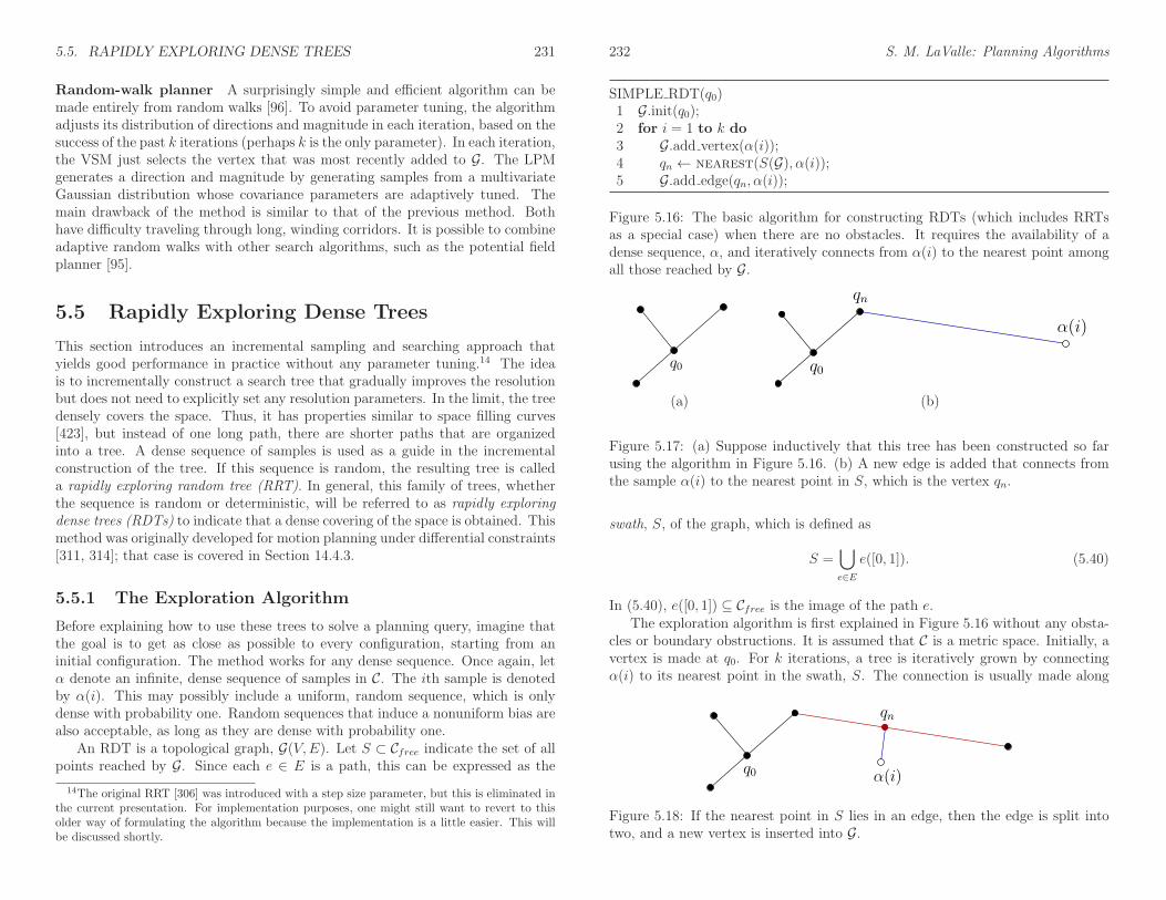
5.5. RAPIDLY EXPLORING DENSE TREES 231
Random-walk planner A surprisingly simple and efficient algorithm can bemade entirely from random walks [96]. To avoid parameter tuning, the algorithmadjusts its distribution of directions and magnitude in each iteration, based on thesuccess of the past k iterations (perhaps k is the only parameter). In each iteration,the VSM just selects the vertex that was most recently added to G. The LPMgenerates a direction and magnitude by generating samples from a multivariateGaussian distribution whose covariance parameters are adaptively tuned. Themain drawback of the method is similar to that of the previous method. Bothhave difficulty traveling through long, winding corridors. It is possible to combineadaptive random walks with other search algorithms, such as the potential fieldplanner [95].
5.5 Rapidly Exploring Dense Trees
This section introduces an incremental sampling and searching approach thatyields good performance in practice without any parameter tuning.14 The ideais to incrementally construct a search tree that gradually improves the resolutionbut does not need to explicitly set any resolution parameters. In the limit, the treedensely covers the space. Thus, it has properties similar to space filling curves[423], but instead of one long path, there are shorter paths that are organizedinto a tree. A dense sequence of samples is used as a guide in the incrementalconstruction of the tree. If this sequence is random, the resulting tree is calleda rapidly exploring random tree (RRT). In general, this family of trees, whetherthe sequence is random or deterministic, will be referred to as rapidly exploringdense trees (RDTs) to indicate that a dense covering of the space is obtained. Thismethod was originally developed for motion planning under differential constraints[311, 314]; that case is covered in Section 14.4.3.
5.5.1 The Exploration Algorithm
Before explaining how to use these trees to solve a planning query, imagine thatthe goal is to get as close as possible to every configuration, starting from aninitial configuration. The method works for any dense sequence. Once again, letα denote an infinite, dense sequence of samples in C. The ith sample is denotedby α(i). This may possibly include a uniform, random sequence, which is onlydense with probability one. Random sequences that induce a nonuniform bias arealso acceptable, as long as they are dense with probability one.
An RDT is a topological graph, G(V,E). Let S ⊂ Cfree indicate the set of allpoints reached by G. Since each e ∈ E is a path, this can be expressed as the
14The original RRT [306] was introduced with a step size parameter, but this is eliminated inthe current presentation. For implementation purposes, one might still want to revert to thisolder way of formulating the algorithm because the implementation is a little easier. This willbe discussed shortly.
232 S. M. LaValle: Planning Algorithms
SIMPLE RDT(q0)1 G.init(q0);2 for i = 1 to k do3 G.add vertex(α(i));4 qn ← nearest(S(G), α(i));5 G.add edge(qn, α(i));
Figure 5.16: The basic algorithm for constructing RDTs (which includes RRTsas a special case) when there are no obstacles. It requires the availability of adense sequence, α, and iteratively connects from α(i) to the nearest point amongall those reached by G.
q0
qn
α(i)
q0
(a) (b)
Figure 5.17: (a) Suppose inductively that this tree has been constructed so farusing the algorithm in Figure 5.16. (b) A new edge is added that connects fromthe sample α(i) to the nearest point in S, which is the vertex qn.
swath, S, of the graph, which is defined as
S =⋃
e∈Ee([0, 1]). (5.40)
In (5.40), e([0, 1]) ⊆ Cfree is the image of the path e.The exploration algorithm is first explained in Figure 5.16 without any obsta-
cles or boundary obstructions. It is assumed that C is a metric space. Initially, avertex is made at q0. For k iterations, a tree is iteratively grown by connectingα(i) to its nearest point in the swath, S. The connection is usually made along
qn
α(i)q0
Figure 5.18: If the nearest point in S lies in an edge, then the edge is split intotwo, and a new vertex is inserted into G.
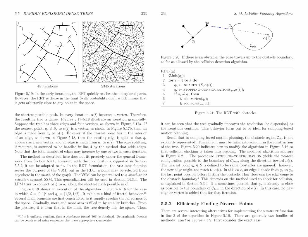
5.5. RAPIDLY EXPLORING DENSE TREES 233
45 iterations 2345 iterations
Figure 5.19: In the early iterations, the RRT quickly reaches the unexplored parts.However, the RRT is dense in the limit (with probability one), which means thatit gets arbitrarily close to any point in the space.
the shortest possible path. In every iteration, α(i) becomes a vertex. Therefore,the resulting tree is dense. Figures 5.17–5.18 illustrate an iteration graphically.Suppose the tree has three edges and four vertices, as shown in Figure 5.17a. Ifthe nearest point, qn ∈ S, to α(i) is a vertex, as shown in Figure 5.17b, then anedge is made from qn to α(i). However, if the nearest point lies in the interiorof an edge, as shown in Figure 5.18, then the existing edge is split so that qnappears as a new vertex, and an edge is made from qn to α(i). The edge splitting,if required, is assumed to be handled in line 4 by the method that adds edges.Note that the total number of edges may increase by one or two in each iteration.
The method as described here does not fit precisely under the general frame-work from Section 5.4.1; however, with the modifications suggested in Section5.5.2, it can be adapted to fit. In the RDT formulation, the nearest functionserves the purpose of the VSM, but in the RDT, a point may be selected fromanywhere in the swath of the graph. The VSM can be generalized to a swath-pointselection method, SSM. This generalization will be used in Section 14.3.4. TheLPM tries to connect α(i) to qn along the shortest path possible in C.
Figure 5.19 shows an execution of the algorithm in Figure 5.16 for the casein which C = [0, 1]2 and q0 = (1/2, 1/2). It exhibits a kind of fractal behavior.15
Several main branches are first constructed as it rapidly reaches the far corners ofthe space. Gradually, more and more area is filled in by smaller branches. Fromthe pictures, it is clear that in the limit, the tree densely fills the space. Thus,
15If α is uniform, random, then a stochastic fractal [303] is obtained. Deterministic fractalscan be constructed using sequences that have appropriate symmetries.
234 S. M. LaValle: Planning Algorithms
qn
q0
Cobs
qs
α(i)
Figure 5.20: If there is an obstacle, the edge travels up to the obstacle boundary,as far as allowed by the collision detection algorithm.
RDT(q0)1 G.init(q0);2 for i = 1 to k do3 qn ← nearest(S, α(i));4 qs ← stopping-configuration(qn,α(i));5 if qs 6= qn then6 G.add vertex(qs);7 G.add edge(qn, qs);
Figure 5.21: The RDT with obstacles.
it can be seen that the tree gradually improves the resolution (or dispersion) asthe iterations continue. This behavior turns out to be ideal for sampling-basedmotion planning.
Recall that in sampling-based motion planning, the obstacle region Cobs is notexplicitly represented. Therefore, it must be taken into account in the constructionof the tree. Figure 5.20 indicates how to modify the algorithm in Figure 5.16 sothat collision checking is taken into account. The modified algorithm appearsin Figure 5.21. The procedure stopping-configuration yields the nearestconfiguration possible to the boundary of Cfree, along the direction toward α(i).The nearest point qn ∈ S is defined to be same (obstacles are ignored); however,the new edge might not reach to α(i). In this case, an edge is made from qn to qs,the last point possible before hitting the obstacle. How close can the edge come tothe obstacle boundary? This depends on the method used to check for collision,as explained in Section 5.3.4. It is sometimes possible that qn is already as closeas possible to the boundary of Cfree in the direction of α(i). In this case, no newedge or vertex is added that for that iteration.
5.5.2 Efficiently Finding Nearest Points
There are several interesting alternatives for implementing the nearest functionin line 3 of the algorithm in Figure 5.16. There are generally two families ofmethods: exact or approximate. First consider the exact case.

5.5. RAPIDLY EXPLORING DENSE TREES 235
Exact solutions Suppose that all edges in G are line segments in Rm for somedimension m ≥ n. An edge that is generated early in the construction process willbe split many times in later iterations. For the purposes of finding the nearestpoint in S, however, it is best to handle this as a single segment. For example, seethe three large branches that extend from the root in Figure 5.19. As the numberof points increases, the benefit of agglomerating the segments increases. Let eachof these agglomerated segments be referred to as a supersegment. To implementnearest, a primitive is needed that computes the distance between a point and aline segment. This can be performed in constant time with simple vector calculus.Using this primitive, nearest is implemented by iterating over all supersegmentsand taking the point with minimum distance among all of them. It may be possibleto improve performance by building hierarchical data structures that can eliminatelarge sets of supersegments, but this remains to be seen experimentally.
In some cases, the edges of G may not be line segments. For example, the short-est paths between two points in SO(3) are actually circular arcs along S3. Onepossible solution is to maintain a separate parameterization of C for the purposesof computing the nearest function. For example, SO(3) can be represented as[0, 1]3/ ∼, by making the appropriate identifications to obtain RP3. Straight-linesegments can then be used. The problem is that the resulting metric is not con-sistent with the Haar measure, which means that an accidental bias would result.Another option is to tightly enclose S3 in a 4D cube. Every point on S3 can bemapped outward onto a cube face. Due to antipodal identification, only four ofthe eight cube faces need to be used to obtain a bijection between the set of allrotation and the cube surface. Linear interpolation can be used along the cubefaces, as long as both points remain on the same face. If the points are on differentfaces, then two line segments can be used by bending the shortest path aroundthe corner between the two faces. This scheme will result in less distortion thanmapping SO(3) to [0, 1]3/ ∼; however, some distortion will still exist.
Another approach is to avoid distortion altogether and implement primitivesthat can compute the distance between a point and a curve. In the case of SO(3),a primitive is needed that can find the distance between a circular arc in Rm
and a point in Rm. This might not be too difficult, but if the curves are morecomplicated, then an exact implementation of the nearest function may be tooexpensive computationally.
Approximate solutions Approximate solutions are much easier to construct,however, a resolution parameter is introduced. Each path segment can be approx-imated by inserting intermediate vertices along long segments, as shown in Figure5.22. The intermediate vertices should be added each time a new sample, α(i),is inserted into G. A parameter ∆q can be defined, and intermediate samples areinserted to ensure that no two consecutive vertices in G are ever further than ∆qfrom each other. Using intermediate vertices, the interiors of the edges in G areignored when finding the nearest point in S. The approximate computation of
236 S. M. LaValle: Planning Algorithms
qn
q0 α(i)
Figure 5.22: For implementation ease, intermediate vertices can be inserted toavoid checking for closest points along line segments. The trade-off is that thenumber of vertices is increased dramatically.
13
12
14
118
910
7
4
5
6
2 3
1
7
8
3 1 10 11
2 4 6 9 13 14
12
5
Figure 5.23: A Kd-tree can be used for efficient nearest-neighbor computations.
nearest is performed by finding the closest vertex to α(i) in G. This approachis by far the simplest to implement. It also fits precisely under the incrementalsampling and searching framework from Section 5.4.1.
When using intermediate vertices, the trade-offs are clear. The computationtime for each evaluation of nearest is linear in the number of vertices. Increasingthe number of vertices improves the quality of the approximation, but it alsodramatically increases the running time. One way to recover some of this cost isto insert the vertices into an efficient data structure for nearest-neighbor searching.One of the most practical and widely used data structures is the Kd-tree [146, 183,391]. A depiction is shown in Figure 5.23 for 14 points in R2. The Kd-tree canbe considered as a multi-dimensional generalization of a binary search tree. TheKd-tree is constructed for points, P , in R2 as follows. Initially, sort the pointswith respect to the x coordinate. Take the median point, p ∈ P , and divideP into two sets, depending on which side of a vertical line through p the otherpoints fall. For each of the two sides, sort the points by the y coordinate and findtheir medians. Points are divided at this level based on whether they are aboveor below horizontal lines. At the next level of recursion, vertical lines are usedagain, followed by horizontal again, and so on. The same idea can be applied inRn by cycling through the n coordinates, instead of alternating between x and y,to form the divisions. In [38], the Kd-tree is extended to topological spaces thatarise in motion planning and is shown to yield good performance for RRTs andsampling-based roadmaps. A Kd-tree of k points can be constructed in O(nk lg k)time. Topological identifications must be carefully considered when traversing

5.5. RAPIDLY EXPLORING DENSE TREES 237
the tree. To find the nearest point in the tree to some given point, the queryalgorithm descends to a leaf vertex whose associated region contains the querypoint, finds all distances from the data points in this leaf to the query point, andpicks the closest one. Next, it recursively visits those surrounding leaf verticesthat are further from the query point than the closest point found so far [36, 38].The nearest point can be found in time logarithmic in k.
Unfortunately, these bounds hide a constant that increases exponentially withthe dimension, n. In practice, the Kd-tree is useful in motion planning for prob-lems of up to about 20 dimensions. After this, the performance usually degradestoo much. As an empirical rule, if there are more than 2n points, then the Kd-treeshould be more efficient than naive nearest neighbors. In general, the trade-offsmust be carefully considered in a particular application to determine whether ex-act solutions, approximate solutions with naive nearest-neighbor computations,or approximate solutions with Kd-trees will be more efficient. There is also theissue of implementation complexity, which probably has caused most people toprefer the approximate solution with naive nearest-neighbor computations.
5.5.3 Using the Trees for Planning
So far, the discussion has focused on exploring Cfree, but this does not solve aplanning query by itself. RRTs and RDTs can be used in many ways in plan-ning algorithms. For example, they could be used to escape local minima in therandomized potential field planner of Section 5.4.3.
Single-tree search A reasonably efficient planner can be made by directly usingthe algorithm in Figure 5.21 to grow a tree from qI and periodically check whetherit is possible to connect the RDT to qG. An easy way to achieve this is to startwith a dense sequence α and periodically insert qG at regularly spaced intervals.For example, every 100th sample could be qG. Each time this sample is reached,an attempt is made to reach qG from the closest vertex in the RDT. If the samplesequence is random, which generates an RRT, then the following modificationworks well. In each iteration, toss a biased coin that has probability 99/100 ofbeing heads and 1/100 of being tails. If the result is heads, then set α(i), to bethe next element of the pseudorandom sequence; otherwise, set α(i) = qG. Thisforces the RRT to occasionally attempt to make a connection to the goal, qG. Ofcourse, 1/100 is arbitrary, but it is in a range that works well experimentally. If thebias is too strong, then the RRT becomes too greedy like the randomized potentialfield. If the bias is not strong enough, then there is no incentive to connect the treeto qG. An alternative is to consider other dense, but not necessarily nonuniformsequences in C. For example, in the case of random sampling, the probabilitydensity function could contain a gentle bias towards the goal. Choosing such abias is a difficult heuristic problem; therefore, such a technique should be usedwith caution (or avoided altogether).
238 S. M. LaValle: Planning Algorithms
RDT BALANCED BIDIRECTIONAL(qI , qG)1 Ta.init(qI); Tb.init(qG);2 for i = 1 to K do3 qn ← nearest(Sa, α(i));4 qs ← stopping-configuration(qn,α(i));5 if qs 6= qn then6 Ta.add vertex(qs);7 Ta.add edge(qn, qs);8 q′n ← nearest(Sb, qs);9 q′s ← stopping-configuration(q′n,qs);10 if q′s 6= q′n then11 Tb.add vertex(q′s);12 Tb.add edge(q′n, q
′s);
13 if q′s = qs then return SOLUTION;14 if |Tb| > |Ta| then SWAP(Ta, Tb);15 return FAILURE
Figure 5.24: A bidirectional RDT-based planner.
Balanced, bidirectional search Much better performance can usually be ob-tained by growing two RDTs, one from qI and the other from qG. This is particu-larly valuable for escaping one of the bug traps, as mentioned in Section 5.4.1. Fora grid search, it is straightforward to implement a bidirectional search that en-sures that the two trees meet. For the RDT, special considerations must be madeto ensure that the two trees will connect while retaining their “rapidly exploring”property. One additional idea is to make sure that the bidirectional search isbalanced [293], which ensures that both trees are the same size.
Figure 5.24 gives an outline of the algorithm. The graph G is decomposedinto two trees, denoted by Ta and Tb. Initially, these trees start from qI andqG, respectively. After some iterations, Ta and Tb are swapped; therefore, keep inmind that Ta is not always the tree that contains qI . In each iteration, Ta is grownexactly the same way as in one iteration of the algorithm in Figure 5.16. If a newvertex, qs, is added to Ta, then an attempt is made in lines 10–12 to extend Tb.Rather than using α(i) to extend Tb, the new vertex qs of Ta is used. This causesTb to try to grow toward Ta. If the two connect, which is tested in line 13, then asolution has been found.
Line 14 represents an important step that balances the search. This is partic-ularly important for a problem such as the bug trap shown in Figure 5.13b or thepuzzle shown in Figure 1.2. If one of the trees is having trouble exploring, thenit makes sense to focus more energy on it. Therefore, new exploration is alwaysperformed for the smaller tree. How is “smaller” defined? A simple criterion is touse the total number of vertices. Another reasonable criterion is to use the totallength of all segments in the tree.

5.6. ROADMAP METHODS FOR MULTIPLE QUERIES 239
An unbalanced bidirectional search can instead be made by forcing the treesto be swapped in every iteration. Once the trees are swapped, then the roles arereversed. For example, after the first swap, Tb is extended in the same way asan integration in Figure 5.16, and if a new vertex qs is added then an attempt ismade to connect Ta to qs.
One important concern exists when α is deterministic. It might be possiblethat even though α is dense, when the samples are divided among the trees, eachmay not receive a dense set. If each uses its own deterministic sequence, then thisproblem can be avoided. In the case of making a bidirectional RRT planner, thesame (pseudo)random sequence can be used for each tree without encounteringsuch troubles.
More than two trees If a dual-tree approach offers advantages over a singletree, then it is natural to ask whether growing three or more RDTs might beeven better. This is particularly helpful for problems like the double bug trap inFigure 5.13c. New trees can be grown from parts of C that are difficult to reach.Controlling the number of trees and determining when to attempt connectionsbetween them is difficult. Some interesting recent work has been done in thisdirection [54, 453, 454].
These additional trees could be started at arbitrary (possibly random) configu-rations. As more trees are considered, a complicated decision problem arises. Thecomputation time must be divided between attempting to explore the space andattempting to connect trees to each other. It is also not clear which connectionsshould be attempted. Many research issues remain in the development of this andother RRT-based planners. A limiting case would be to start a new tree fromevery sample in α(i) and to try to connect nearby trees whenever possible. Thisapproach results in a graph that covers the space in a nice way that is independentof the query. This leads to the main topic of the next section.
5.6 Roadmap Methods for Multiple Queries
Previously, it was assumed that a single initial-goal pair was given to the planningalgorithm. Suppose now that numerous initial-goal queries will be given to thealgorithm, while keeping the robot model and obstacles fixed. This leads to amultiple-query version of the motion planning problem. In this case, it makes senseto invest substantial time to preprocess the models so that future queries can beanswered efficiently. The goal is to construct a topological graph called a roadmap,which efficiently solves multiple initial-goal queries. Intuitively, the paths on theroadmap should be easy to reach from each of qI and qG, and the graph canbe quickly searched for a solution. The general framework presented here wasmainly introduced in [265] under the name probabilistic roadmaps (PRMs). Theprobabilistic aspect, however, is not important to the method. Therefore, we call
240 S. M. LaValle: Planning Algorithms
BUILD ROADMAP1 G.init(); i← 0;2 while i < N3 if α(i) ∈ Cfree then4 G.add vertex(α(i)); i← i+ 1;5 for each q ∈ neighborhood(α(i),G)6 if ((not G.same component(α(i), q)) and connect(α(i), q)) then7 G.add edge(α(i), q);
Figure 5.25: The basic construction algorithm for sampling-based roadmaps. Notethat i is not incremented if α(i) is in collision. This forces i to correctly count thenumber of vertices in the roadmap.
this family of methods sampling-based roadmaps. This distinguishes them fromcombinatorial roadmaps, which will appear in Chapter 6.
5.6.1 The Basic Method
Once again, let G(V,E) represent a topological graph in which V is a set of verticesand E is the set of paths that map into Cfree. Under the multiple-query philosophy,motion planning is divided into two phases of computation:
Preprocessing Phase: During the preprocessing phase, substantial effortis invested to build G in a way that is useful for quickly answering futurequeries. For this reason, it is called a roadmap, which in some sense shouldbe accessible from every part of Cfree.
Query Phase: During the query phase, a pair, qI and qG, is given. Eachconfiguration must be connected easily to G using a local planner. Followingthis, a discrete search is performed using any of the algorithms in Section2.2 to obtain a sequence of edges that forms a path from qI to qG.
Generic preprocessing phase Figure 5.25 presents an outline of the basicpreprocessing phase, and Figure 5.26 illustrates the algorithm. As seen throughoutthis chapter, the algorithm utilizes a uniform, dense sequence α. In each iteration,the algorithm must check whether α(i) ∈ Cfree. If α(i) ∈ Cobs, then it mustcontinue to iterate until a collision-free sample is obtained. Once α(i) ∈ Cfree,then in line 4 it is inserted as a vertex of G. The next step is to try to connect α(i)to some nearby vertices, q, of G. Each connection is attempted by the connect
function, which is a typical LPM (local planning method) from Section 5.4.1.In most implementations, this simply tests the shortest path between α(i) andq. Experimentally, it seems most efficient to use the multi-resolution, van derCorput–based method described at the end of Section 5.3.4 [191]. Instead of theshortest path, it is possible to use more sophisticated connection methods, such
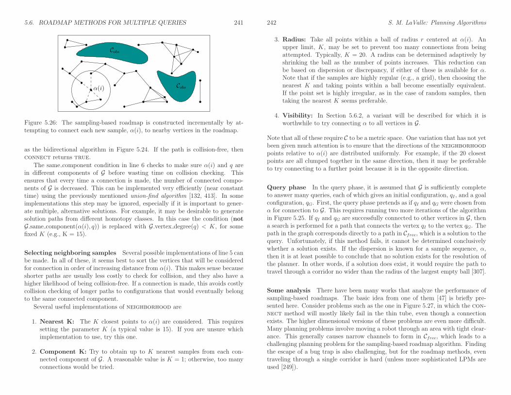
5.6. ROADMAP METHODS FOR MULTIPLE QUERIES 241
α(i)
Cobs
Cobs
Figure 5.26: The sampling-based roadmap is constructed incrementally by at-tempting to connect each new sample, α(i), to nearby vertices in the roadmap.
as the bidirectional algorithm in Figure 5.24. If the path is collision-free, thenconnect returns true.
The same component condition in line 6 checks to make sure α(i) and q arein different components of G before wasting time on collision checking. Thisensures that every time a connection is made, the number of connected compo-nents of G is decreased. This can be implemented very efficiently (near constanttime) using the previously mentioned union-find algorithm [132, 413]. In someimplementations this step may be ignored, especially if it is important to gener-ate multiple, alternative solutions. For example, it may be desirable to generatesolution paths from different homotopy classes. In this case the condition (notG.same component(α(i), q)) is replaced with G.vertex degree(q) < K, for somefixed K (e.g., K = 15).
Selecting neighboring samples Several possible implementations of line 5 canbe made. In all of these, it seems best to sort the vertices that will be consideredfor connection in order of increasing distance from α(i). This makes sense becauseshorter paths are usually less costly to check for collision, and they also have ahigher likelihood of being collision-free. If a connection is made, this avoids costlycollision checking of longer paths to configurations that would eventually belongto the same connected component.
Several useful implementations of neighborhood are
1. Nearest K: The K closest points to α(i) are considered. This requiressetting the parameter K (a typical value is 15). If you are unsure whichimplementation to use, try this one.
2. Component K: Try to obtain up to K nearest samples from each con-nected component of G. A reasonable value is K = 1; otherwise, too manyconnections would be tried.
242 S. M. LaValle: Planning Algorithms
3. Radius: Take all points within a ball of radius r centered at α(i). Anupper limit, K, may be set to prevent too many connections from beingattempted. Typically, K = 20. A radius can be determined adaptively byshrinking the ball as the number of points increases. This reduction canbe based on dispersion or discrepancy, if either of these is available for α.Note that if the samples are highly regular (e.g., a grid), then choosing thenearest K and taking points within a ball become essentially equivalent.If the point set is highly irregular, as in the case of random samples, thentaking the nearest K seems preferable.
4. Visibility: In Section 5.6.2, a variant will be described for which it isworthwhile to try connecting α to all vertices in G.
Note that all of these require C to be a metric space. One variation that has not yetbeen given much attention is to ensure that the directions of the neighborhoodpoints relative to α(i) are distributed uniformly. For example, if the 20 closestpoints are all clumped together in the same direction, then it may be preferableto try connecting to a further point because it is in the opposite direction.
Query phase In the query phase, it is assumed that G is sufficiently completeto answer many queries, each of which gives an initial configuration, qI , and a goalconfiguration, qG. First, the query phase pretends as if qI and qG were chosen fromα for connection to G. This requires running two more iterations of the algorithmin Figure 5.25. If qI and qG are successfully connected to other vertices in G, thena search is performed for a path that connects the vertex qI to the vertex qG. Thepath in the graph corresponds directly to a path in Cfree, which is a solution to thequery. Unfortunately, if this method fails, it cannot be determined conclusivelywhether a solution exists. If the dispersion is known for a sample sequence, α,then it is at least possible to conclude that no solution exists for the resolution ofthe planner. In other words, if a solution does exist, it would require the path totravel through a corridor no wider than the radius of the largest empty ball [307].
Some analysis There have been many works that analyze the performance ofsampling-based roadmaps. The basic idea from one of them [47] is briefly pre-sented here. Consider problems such as the one in Figure 5.27, in which the con-nect method will mostly likely fail in the thin tube, even though a connectionexists. The higher dimensional versions of these problems are even more difficult.Many planning problems involve moving a robot through an area with tight clear-ance. This generally causes narrow channels to form in Cfree, which leads to achallenging planning problem for the sampling-based roadmap algorithm. Findingthe escape of a bug trap is also challenging, but for the roadmap methods, eventraveling through a single corridor is hard (unless more sophisticated LPMs areused [249]).
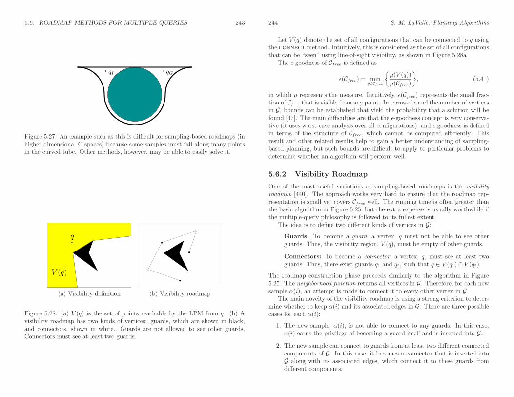
5.6. ROADMAP METHODS FOR MULTIPLE QUERIES 243
qGqI
Figure 5.27: An example such as this is difficult for sampling-based roadmaps (inhigher dimensional C-spaces) because some samples must fall along many pointsin the curved tube. Other methods, however, may be able to easily solve it.
V (q)
q
(a) Visibility definition (b) Visibility roadmap
Figure 5.28: (a) V (q) is the set of points reachable by the LPM from q. (b) Avisibility roadmap has two kinds of vertices: guards, which are shown in black,and connectors, shown in white. Guards are not allowed to see other guards.Connectors must see at least two guards.
244 S. M. LaValle: Planning Algorithms
Let V (q) denote the set of all configurations that can be connected to q usingthe connectmethod. Intuitively, this is considered as the set of all configurationsthat can be “seen” using line-of-sight visibility, as shown in Figure 5.28a
The ǫ-goodness of Cfree is defined as
ǫ(Cfree) = minq∈Cfree
µ(V (q))
µ(Cfree)
, (5.41)
in which µ represents the measure. Intuitively, ǫ(Cfree) represents the small frac-tion of Cfree that is visible from any point. In terms of ǫ and the number of verticesin G, bounds can be established that yield the probability that a solution will befound [47]. The main difficulties are that the ǫ-goodness concept is very conserva-tive (it uses worst-case analysis over all configurations), and ǫ-goodness is definedin terms of the structure of Cfree, which cannot be computed efficiently. Thisresult and other related results help to gain a better understanding of sampling-based planning, but such bounds are difficult to apply to particular problems todetermine whether an algorithm will perform well.
5.6.2 Visibility Roadmap
One of the most useful variations of sampling-based roadmaps is the visibilityroadmap [440]. The approach works very hard to ensure that the roadmap rep-resentation is small yet covers Cfree well. The running time is often greater thanthe basic algorithm in Figure 5.25, but the extra expense is usually worthwhile ifthe multiple-query philosophy is followed to its fullest extent.
The idea is to define two different kinds of vertices in G:Guards: To become a guard, a vertex, q must not be able to see otherguards. Thus, the visibility region, V (q), must be empty of other guards.
Connectors: To become a connector, a vertex, q, must see at least twoguards. Thus, there exist guards q1 and q2, such that q ∈ V (q1) ∩ V (q2).
The roadmap construction phase proceeds similarly to the algorithm in Figure5.25. The neighborhood function returns all vertices in G. Therefore, for each newsample α(i), an attempt is made to connect it to every other vertex in G.
The main novelty of the visibility roadmap is using a strong criterion to deter-mine whether to keep α(i) and its associated edges in G. There are three possiblecases for each α(i):
1. The new sample, α(i), is not able to connect to any guards. In this case,α(i) earns the privilege of becoming a guard itself and is inserted into G.
2. The new sample can connect to guards from at least two different connectedcomponents of G. In this case, it becomes a connector that is inserted intoG along with its associated edges, which connect it to these guards fromdifferent components.

5.6. ROADMAP METHODS FOR MULTIPLE QUERIES 245
3. Neither of the previous two conditions were satisfied. This means that thesample could only connect to guards in the same connected component. Inthis case, α(i) is discarded.
The final condition causes a dramatic reduction in the number of roadmap vertices.One problem with this method is that it does not allow guards to be deleted in
favor of better guards that might appear later. The placement of guards dependsstrongly on the order in which samples appear in α. The method may performpoorly if guards are not positioned well early in the sequence. It would be betterto have an adaptive scheme in which guards could be reassigned in later iterationsas better positions become available. Accomplishing this efficiently remains anopen problem. Note the algorithm is still probabilistically complete using randomsampling or resolution complete if α is dense, even though many samples arerejected.
5.6.3 Heuristics for Improving Roadmaps
The quest to design a good roadmap through sampling has spawned many heuris-tic approaches to sampling and making connections in roadmaps. Most of theseexploit properties that are specific to the shape of the C-space and/or the partic-ular geometry and kinematics of the robot and obstacles. The emphasis is usuallyon finding ways to dramatically reduce the number or required samples. Severalof these methods are briefly described here.
Vertex enhancement [265] This heuristic strategy focuses effort on verticesthat were difficult to connect to other vertices in the roadmap construction algo-rithm in Figure 5.25. A probability distribution, P (v), is defined over the verticesv ∈ V . A number of iterations are then performed in which a vertex is sampledfrom V according to P (v), and then some random motions are performed from vto try to reach new configurations. These new configurations are added as ver-tices, and attempts are made to connect them to other vertices, as selected bythe neighborhood function in an ordinary iteration of the algorithm in Figure5.25. A recommended heuristic [265] for defining P (v) is to define a statistic foreach v as nf/(nt + 1), in which nt is the total number of connections attemptedfor v, and nf is the number of times these attempts failed. The probability P (v)is assigned as nf/(nt +1)m, in which m is the sum of the statistics over all v ∈ V(this normalizes the statistics to obtain a valid probability distribution).
Sampling on the Cfree boundary [16, 20] This scheme is based on the intu-ition that it is sometimes better to sample along the boundary, ∂Cfree, rather thanwaste samples on large areas of Cfree that might be free of obstacles. Figure 5.29ashows one way in which this can be implemented. For each sample of α(i) thatfalls into Cobs, a number of random directions are chosen in C; these directions canbe sampled using the Sn sampling method from Section 5.2.2. For each direction,
246 S. M. LaValle: Planning Algorithms
1α(i)
Cobs
4
23
Cobs Cobs
(a) (b)
Figure 5.29: (a) To obtain samples along the boundary, binary search is usedalong random directions from a sample in Cobs. (b) The bridge test finds narrowcorridors by examining a triple of nearby samples along a line.
a binary search is performed to get a sample in Cfree that is as close as possibleto Cobs. The order of point evaluation in the binary search is shown in Figure5.29a. Let τ : [0, 1] denote the path for which τ(0) ∈ Cobs and τ(1) ∈ Cfree. In thefirst step, test the midpoint, τ(1/2). If τ(1/2) ∈ Cfree, this means that ∂Cfree liesbetween τ(0) and τ(1/2); otherwise, it lies between τ(1/2) and τ(1). The nextiteration selects the midpoint of the path segment that contains ∂Cfree. This willbe either τ(1/4) or τ(3/4). The process continues recursively until the desiredresolution is obtained.
Gaussian sampling [72] The Gaussian sampling strategy follows some of thesame motivation for sampling on the boundary. In this case, the goal is to obtainpoints near ∂Cfree by using a Gaussian distribution that biases the samples to becloser to ∂Cfree, but the bias is gentler, as prescribed by the variance parameterof the Gaussian. The samples are generated as follows. Generate one sample,q1 ∈ C, uniformly at random. Following this, generate another sample, q2 ∈ C,according to a Gaussian with mean q1; the distribution must be adapted for anytopological identifications and/or boundaries of C. If one of q1 or q2 lies in Cfreeand the other lies in Cobs, then the one that lies in Cfree is kept as a vertex in theroadmap. For some examples, this dramatically prunes the number of requiredvertices.
Bridge-test sampling [241] The Gaussian sampling strategy decides to keep apoint based in part on testing a pair of samples. This idea can be carried one stepfurther to obtain a bridge test, which uses three samples along a line segment.If the samples are arranged as shown in Figure 5.29b, then the middle samplebecomes a roadmap vertex. This is based on the intuition that narrow corridorsare thin in at least one direction. The bridge test indicates that a point lies in athin corridor, which is often an important place to locate a vertex.
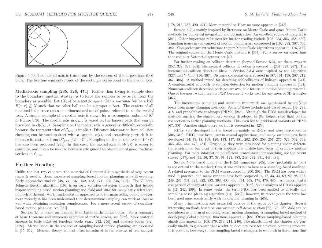
5.6. ROADMAP METHODS FOR MULTIPLE QUERIES 247
Figure 5.30: The medial axis is traced out by the centers of the largest inscribedballs. The five line segments inside of the rectangle correspond to the medial axis.
Medial-axis sampling [235, 326, 474] Rather than trying to sample closeto the boundary, another strategy is to force the samples to be as far from theboundary as possible. Let (X, ρ) be a metric space. Let a maximal ball be a ballB(x, r) ⊆ X such that no other ball can be a proper subset. The centers of allmaximal balls trace out a one-dimensional set of points referred to as the medialaxis. A simple example of a medial axis is shown for a rectangular subset of R2
in Figure 5.30. The medial axis in Cfree is based on the largest balls that can beinscribed in cl(Cfree). Sampling on the medial axis is generally difficult, especiallybecause the representation of Cfree is implicit. Distance information from collisionchecking can be used to start with a sample, α(i), and iteratively perturb it toincrease its distance from ∂Cfree [326, 474]. Sampling on the medial axis of W \Ohas also been proposed [235]. In this case, the medial axis in W \ O is easier tocompute, and it can be used to heuristically guide the placement of good roadmapvertices in Cfree.
Further Reading
Unlike the last two chapters, the material of Chapter 5 is a synthesis of very recentresearch results. Some aspects of sampling-based motion planning are still evolving.Early approaches include [48, 77, 107, 152, 153, 171, 172, 345, 392]. The Gilbert-Johnson-Keerthi algorithm [199] is an early collision detection approach that helpedinspire sampling-based motion planning; see [245] and [304] for many early references.In much of the early work, randomization appeared to be the main selling point; however,more recently it has been understood that deterministic sampling can work at least aswell while obtaining resolution completeness. For a more recent survey of sampling-based motion planning, see [331].
Section 5.1 is based on material from basic mathematics books. For a summaryof basic theorems and numerous examples of metric spaces, see [362]. More materialappears in basic point-set topology books (e.g., [232, 256]) and analysis books (e.g.,[178]). Metric issues in the context of sampling-based motion planning are discussedin [15, 312]. Measure theory is most often introduced in the context of real analysis
248 S. M. LaValle: Planning Algorithms
[178, 215, 287, 420, 421]. More material on Haar measure appears in [215].
Section 5.2 is mainly inspired by literature on Monte Carlo and quasi–Monte Carlomethods for numerical integration and optimization. An excellent source of material is[381]. Other important references for further reading include [105, 283, 353, 458, 459].Sampling issues in the context of motion planning are considered in [192, 292, 307, 330,482]. Comprehensive introductions to pure Monte Carlo algorithms appear in [176, 259].The original source for the Monte Carlo method is [361]. For a survey on algorithmsthat compute Voronoi diagrams, see [40].
For further reading on collision detection (beyond Section 5.3), see the surveys in[252, 328, 329, 368]. Hierarchical collision detection is covered in [207, 329, 367]. Theincremental collision detection ideas in Section 5.3.3 were inspired by the algorithm[327] and V-Clip [136, 367]. Distance computation is covered in [87, 161, 198, 207, 212,367, 406]. A method suited for detecting self-collisions of linkages appears in [341].A combinatorial approach to collision detection for motion planning appears in [431].Numerous collision detection packages are available for use in motion planning research.One of the most widely used is PQP because it works well for any mess of 3D triangles[463].
The incremental sampling and searching framework was synthesized by unifyingideas from many planning methods. Some of these include grid-based search [49, 289,318] and probabilistic roadmaps (PRMs) [265]. Although the PRM was developed formultiple queries, the single-query version developed in [69] helped shed light on theconnection to earlier planning methods. This even led to grid-based variants of PRMs[67, 307]. Another single-query variant is presented in [425].
RDTs were developed in the literature mainly as RRTs, and were introduced in[306, 313]. RRTs have been used in several applications, and many variants have beendeveloped [54, 75, 78, 109, 120, 133, 147, 181, 202, 255, 258, 257, 275, 324, 332, 333,453, 454, 464, 479, 481]. Originally, they were developed for planning under differen-tial constraints, but most of their applications to date have been for ordinary motionplanning. For more information on efficient nearest-neighbor searching, see the recentsurvey [247], and [35, 36, 37, 38, 61, 123, 183, 248, 282, 391, 448, 483].
Section 5.6 is based mainly on the PRM framework [265]. The “probabilistic” partis not critical to the method; thus, it was referred to here as a sampling-based roadmap.A related precursor to the PRM was proposed in [200, 201]. The PRM has been widelyused in practice, and many variants have been proposed [1, 17, 43, 44, 69, 82, 98, 133,249, 286, 307, 321, 322, 383, 398, 400, 440, 444, 465, 474, 479, 486]. An experimentalcomparison of many of these variants appears in [192]. Some analysis of PRMs appearsin [47, 242, 299]. In some works, the term PRM has been applied to virtually anysampling-based planning algorithm (e.g., [242]); however, in recent years the term hasbeen used more consistently with its original meaning in [265].
Many other methods and issues fall outside of the scope of this chapter. Severalinteresting methods based on approximate cell decomposition [77, 170, 337, 345] can beconsidered as a form of sampling-based motion planning. A sampling-based method ofdeveloping global potential functions appears in [68]. Other sampling-based planningalgorithms appear in [108, 179, 213, 214, 240]. The algorithms of this chapter are gen-erally unable to guarantee that a solution does not exist for a motion planning problem.It is possible, however, to use sampling-based techniques to establish in finite time that
5.6. ROADMAP METHODS FOR MULTIPLE QUERIES 249
no solution exists [51]. Such a result is called a disconnection proof. Parallelizationissues have also been investigated in the context of sampling-based motion planning[54, 94, 99, 143, 401].
Exercises
1. Prove that the Cartesian product of a metric space is a metric space by taking alinear combination as in (5.4).
2. Prove or disprove: If ρ is a metric, then ρ2 is a metric.
3. Determine whether the following function is a metric on any topological space:X: ρ(x, x′) = 1 is x 6= x′; otherwise, ρ(x, x′) = 0.
4. State and prove whether or not (5.28) yields a metric space on C = SE(3),assuming that the two sets are rigid bodies.
5. The dispersion definition given in (5.19) is based on the worst case. Considerdefining the average dispersion:
δ(P ) =1
µ(X)
∫
Xminp∈Pρ(x, p)dx. (5.42)
Describe a Monte Carlo (randomized) method to approximately evaluate (5.42).
6. Determine the average dispersion (as a function of i) for the van der Corputsequence (base 2) on [0, 1]/ ∼.
7. Show that using the Lebesgue measure on S3 (spreading mass around uniformlyon S3) yields the Haar measure for SO(3).
8. Is the Haar measure useful in selecting an appropriate C-space metric? Explain.
9. Determine an expression for the (worst-case) dispersion of the ith sample in thebase-p (Figure 5.2 shows base-2) van der Corput sequence in [0, 1]/ ∼, in which 0and 1 are identified.
10. Determine the dispersion of the following sequence on [0, 1]. The first point isα(1) = 1. For each i > 1, let ci = ln(2i − 3)/ ln 4 and α(i) = ci − ⌊ci⌋. It turnsout that this sequence achieves the best asymptotic dispersion possible, even interms of the preceding constant. Also, the points are not uniformly distributed.Can you explain why this happens? [It may be helpful to plot the points in thesequence.]
11. Prove that (5.20) holds.
12. Prove that (5.23) holds.
13. Show that for any given set of points in [0, 1]n, a range space R can be designedso that the discrepancy is as close as desired to 1.
250 S. M. LaValle: Planning Algorithms
14. Suppose A is a rigid body in R3 with a fixed orientation specified by a quaternion,h. Suppose that h is perturbed a small amount to obtain another quaternion, h′
(no translation occurs). Construct a good upper bound on distance traveled bypoints on A, expressed in terms of the change in the quaternion.
15. Design combinations of robots and obstacles in W that lead to C-space obstaclesresembling bug traps.
16. How many k-neighbors can there be at most in an n-dimensional grid with 1 ≤k ≤ n?
17. In a high-dimensional grid, it becomes too costly to consider all 3n−1 n-neighbors.It might not be enough to consider only 2n 1-neighbors. Determine a scheme forselecting neighbors that are spatially distributed in a good way, but withoutrequiring too many. For example, what is a good way to select 50 neighbors fora grid in R10?
18. Explain the difference between searching an implicit, high-resolution grid andgrowing search trees directly on the C-space without a grid.
19. Improve the bound in (5.31) by considering the fact that rotating points traceout a circle, instead of a straight line.
20. (Open problem) Prove there are n+1 main branches for an RRT starting from thecenter of an “infinite” n-dimensional ball in Rn. The directions of the branchesalign with the vertices of a regular simplex centered at the initial configuration.
Implementations
21. Implement 2D incremental collision checking for convex polygons to obtain “nearconstant time” performance.
22. Implement the sampling-based roadmap approach. Select an appropriate familyof motion planning problems: 2D rigid bodies, 2D chains of bodies, 3D rigidbodies, etc.
(a) Compare the roadmaps obtained using visibility-based sampling to thoseobtained for the ordinary sampling method.
(b) Study the sensitivity of the method with respect to the particular neigh-
borhood method.
(c) Compare random and deterministic sampling methods.
(d) Use the bridge test to attempt to produce better samples.
23. Implement the balanced, bidirectional RRT planning algorithm.
(a) Study the effect of varying the amount of intermediate vertices created alongedges.

5.6. ROADMAP METHODS FOR MULTIPLE QUERIES 251
(b) Try connecting to the random sample using more powerful descent functions.
(c) Explore the performance gains from using Kd-trees to select nearest neigh-bors.
24. Make an RRT-based planning algorithm that uses more than two trees. Carefullyresolve issues such as the maximum number of allowable trees, when to start atree, and when to attempt connections between trees.
25. Implement both the expansive-space planner and the RRT, and conduct compar-ative experiments on planning problems. For the full set of problems, keep thealgorithm parameters fixed.
26. Implement a sampling-based algorithm that computes collision-free paths for arigid robot that can translate or rotate on any of the flat 2D manifolds shown inFigure 4.5.
252 S. M. LaValle: Planning Algorithms

Chapter 6
Combinatorial Motion Planning
Combinatorial approaches to motion planning find paths through the continuousconfiguration space without resorting to approximations. Due to this property,they are alternatively referred to as exact algorithms. This is in contrast to thesampling-based motion planning algorithms from Chapter 5.
6.1 Introduction
All of the algorithms presented in this chapter are complete, which means thatfor any problem instance (over the space of problems for which the algorithm isdesigned), the algorithm will either find a solution or will correctly report that nosolution exists. By contrast, in the case of sampling-based planning algorithms,weaker notions of completeness were tolerated: resolution completeness and prob-abilistic completeness.
Representation is important When studying combinatorial motion planningalgorithms, it is important to carefully consider the definition of the input. Whatis the representation used for the robot and obstacles? What set of transforma-tions may be applied to the robot? What is the dimension of the world? Arethe robot and obstacles convex? Are they piecewise linear? The specification ofpossible inputs defines a set of problem instances on which the algorithm will op-erate. If the instances have certain convenient properties (e.g., low dimensionality,convex models), then a combinatorial algorithm may provide an elegant, practicalsolution. If the set of instances is too broad, then a requirement of both complete-ness and practical solutions may be unreasonable. Many general formulations ofgeneral motion planning problems are PSPACE-hard1; therefore, such a hope ap-pears unattainable. Nevertheless, there exist general, complete motion planningalgorithms. Note that focusing on the representation is the opposite philosophyfrom sampling-based planning, which hides these issues in the collision detectionmodule.
1This implies NP-hard. An overview of such complexity statements appears in Section 6.5.1.
253
254 S. M. LaValle: Planning Algorithms
Reasons to study combinatorial methods There are generally two goodreasons to study combinatorial approaches to motion planning:
1. In many applications, one may only be interested in a special class of plan-ning problems. For example, the world might be 2D, and the robot mightonly be capable of translation. For many special classes, elegant and ef-ficient algorithms can be developed. These algorithms are complete, donot depend on approximation, and can offer much better performance thansampling-based planning methods, such as those in Chapter 5.
2. It is both interesting and satisfying to know that there are complete algo-rithms for an extremely broad class of motion planning problems. Thus,even if the class of interest does not have some special limiting assumptions,there still exist general-purpose tools and algorithms that can solve it. Thesealgorithms also provide theoretical upper bounds on the time needed to solvemotion planning problems.
Warning: Some methods are impractical Be careful not to make the wrongassumptions when studying the algorithms of this chapter. A few of them are ef-ficient and easy to implement, but many might be neither. Even if an algorithmhas an amazing asymptotic running time, it might be close to impossible to im-plement. For example, one of the most famous algorithms from computationalgeometry can split a simple2 polygon into triangles in O(n) time for a polygonwith n edges [104]. This is so amazing that it was covered in the New YorkTimes, but the algorithm is so complicated that it is doubtful that anyone willever implement it. Sometimes it is preferable to use an algorithm that has worsetheoretical running time but is much easier to understand and implement. Ingeneral, though, it is valuable to understand both kinds of methods and decideon the trade-offs for yourself. It is also an interesting intellectual pursuit to tryto determine how efficiently a problem can be solved, even if the result is mainlyof theoretical interest. This might motivate others to look for simpler algorithmsthat have the same or similar asymptotic running times.
Roadmaps Virtually all combinatorial motion planning approaches construct aroadmap along the way to solving queries. This notion was introduced in Section5.6, but in this chapter stricter requirements are imposed in the roadmap definitionbecause any algorithm that constructs one needs to be complete. Some of thealgorithms in this chapter first construct a cell decomposition of Cfree from whichthe roadmap is consequently derived. Other methods directly construct a roadmapwithout the consideration of cells.
Let G be a topological graph (defined in Example 4.6) that maps into Cfree.Furthermore, let S ⊂ Cfree be the swath, which is set of all points reached by G,
2A polygonal region that has no holes.

6.2. POLYGONAL OBSTACLE REGIONS 255
as defined in (5.40). The graph G is called a roadmap if it satisfies two importantconditions:
1. Accessibility: From any q ∈ Cfree, it is simple and efficient to compute apath τ : [0, 1] → Cfree such that τ(0) = q and τ(1) = s, in which s may beany point in S. Usually, s is the closest point to q, assuming C is a metricspace.
2. Connectivity-preserving: Using the first condition, it is always possibleto connect some qI and qG to some s1 and s2, respectively, in S. The secondcondition requires that if there exists a path τ : [0, 1] → Cfree such thatτ(0) = qI and τ(1) = qG, then there also exists a path τ ′ : [0, 1] → S, suchthat τ ′(0) = s1 and τ
′(1) = s2. Thus, solutions are not missed because G failsto capture the connectivity of Cfree. This ensures that complete algorithmsare developed.
By satisfying these properties, a roadmap provides a discrete representation ofthe continuous motion planning problem without losing any of the original con-nectivity information needed to solve it. A query, (qI , qG), is solved by connectingeach query point to the roadmap and then performing a discrete graph search onG. To maintain completeness, the first condition ensures that any query can beconnected to G, and the second condition ensures that the search always succeedsif a solution exists.
6.2 Polygonal Obstacle Regions
Rather than diving into the most general forms of combinatorial motion plan-ning, it is helpful to first see several methods explained for a case that is easy tovisualize. Several elegant, straightforward algorithms exist for the case in whichC = R2 and Cobs is polygonal. Most of these cannot be directly extended to higherdimensions; however, some of the general principles remain the same. Therefore,it is very instructive to see how combinatorial motion planning approaches work intwo dimensions. There are also applications where these algorithms may directlyapply. One example is planning for a small mobile robot that may be modeled asa point moving in a building that can be modeled with a 2D polygonal floor plan.
After covering representations in Section 6.2.1, Sections 6.2.2–6.2.4 presentthree different algorithms to solve the same problem. The one in Section 6.2.2first performs cell decomposition on the way to building the roadmap, and theones in Sections 6.2.3 and 6.2.4 directly produce a roadmap. The algorithm inSection 6.2.3 computes maximum clearance paths, and the one in Section 6.2.4computes shortest paths (which consequently have no clearance).
256 S. M. LaValle: Planning Algorithms
Figure 6.1: A polygonal model specified by four oriented simple polygons.
6.2.1 Representation
Assume that W = R2; the obstacles, O, are polygonal; and the robot, A, is apolygonal body that is only capable of translation. Under these assumptions, Cobswill be polygonal. For the special case in which A is a point inW , O maps directlyto Cobs without any distortion. Thus, the problems considered in this section mayalso be considered as planning for a point robot. If A is not a point robot, thenthe Minkowski difference, (4.37), of O and A must be computed. For the casein which both A and each component of O are convex, the algorithm in Section4.3.2 can be applied to compute each component of Cobs. In general, both A andO may be nonconvex. They may even contain holes, which results in a Cobs modelsuch as that shown in Figure 6.1. In this case, A and O may be decomposedinto convex components, and the Minkowski difference can be computed for eachpair of components. The decompositions into convex components can actually beperformed by adapting the cell decomposition algorithm that will be presentedin Section 6.2.2. Once the Minkowski differences have been computed, they needto be merged to obtain a representation that can be specified in terms of simplepolygons, such as those in Figure 6.1. An efficient algorithm to perform thismerging is given in Section 2.4 of [146]. It can also be based on many of the sameprinciples as the planning algorithm in Section 6.2.2.
To implement the algorithms described in this section, it will be helpful tohave a data structure that allows convenient access to the information contained
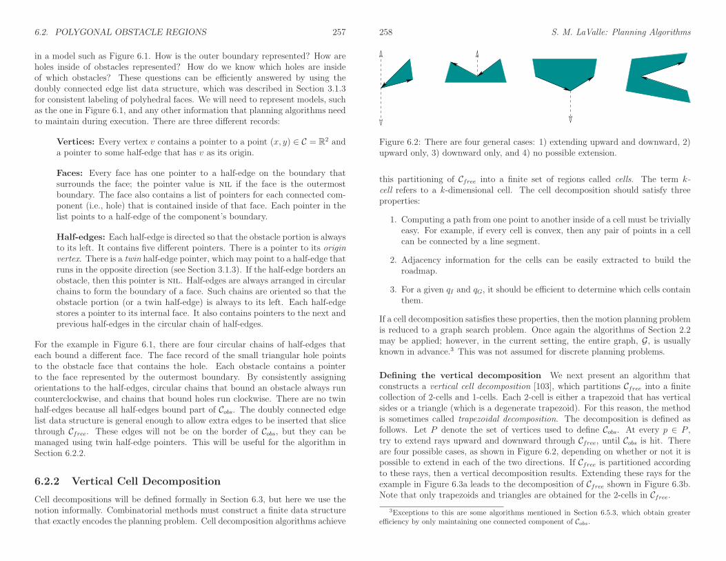
6.2. POLYGONAL OBSTACLE REGIONS 257
in a model such as Figure 6.1. How is the outer boundary represented? How areholes inside of obstacles represented? How do we know which holes are insideof which obstacles? These questions can be efficiently answered by using thedoubly connected edge list data structure, which was described in Section 3.1.3for consistent labeling of polyhedral faces. We will need to represent models, suchas the one in Figure 6.1, and any other information that planning algorithms needto maintain during execution. There are three different records:
Vertices: Every vertex v contains a pointer to a point (x, y) ∈ C = R2 anda pointer to some half-edge that has v as its origin.
Faces: Every face has one pointer to a half-edge on the boundary thatsurrounds the face; the pointer value is nil if the face is the outermostboundary. The face also contains a list of pointers for each connected com-ponent (i.e., hole) that is contained inside of that face. Each pointer in thelist points to a half-edge of the component’s boundary.
Half-edges: Each half-edge is directed so that the obstacle portion is alwaysto its left. It contains five different pointers. There is a pointer to its originvertex. There is a twin half-edge pointer, which may point to a half-edge thatruns in the opposite direction (see Section 3.1.3). If the half-edge borders anobstacle, then this pointer is nil. Half-edges are always arranged in circularchains to form the boundary of a face. Such chains are oriented so that theobstacle portion (or a twin half-edge) is always to its left. Each half-edgestores a pointer to its internal face. It also contains pointers to the next andprevious half-edges in the circular chain of half-edges.
For the example in Figure 6.1, there are four circular chains of half-edges thateach bound a different face. The face record of the small triangular hole pointsto the obstacle face that contains the hole. Each obstacle contains a pointerto the face represented by the outermost boundary. By consistently assigningorientations to the half-edges, circular chains that bound an obstacle always runcounterclockwise, and chains that bound holes run clockwise. There are no twinhalf-edges because all half-edges bound part of Cobs. The doubly connected edgelist data structure is general enough to allow extra edges to be inserted that slicethrough Cfree. These edges will not be on the border of Cobs, but they can bemanaged using twin half-edge pointers. This will be useful for the algorithm inSection 6.2.2.
6.2.2 Vertical Cell Decomposition
Cell decompositions will be defined formally in Section 6.3, but here we use thenotion informally. Combinatorial methods must construct a finite data structurethat exactly encodes the planning problem. Cell decomposition algorithms achieve
258 S. M. LaValle: Planning Algorithms
Figure 6.2: There are four general cases: 1) extending upward and downward, 2)upward only, 3) downward only, and 4) no possible extension.
this partitioning of Cfree into a finite set of regions called cells. The term k-cell refers to a k-dimensional cell. The cell decomposition should satisfy threeproperties:
1. Computing a path from one point to another inside of a cell must be triviallyeasy. For example, if every cell is convex, then any pair of points in a cellcan be connected by a line segment.
2. Adjacency information for the cells can be easily extracted to build theroadmap.
3. For a given qI and qG, it should be efficient to determine which cells containthem.
If a cell decomposition satisfies these properties, then the motion planning problemis reduced to a graph search problem. Once again the algorithms of Section 2.2may be applied; however, in the current setting, the entire graph, G, is usuallyknown in advance.3 This was not assumed for discrete planning problems.
Defining the vertical decomposition We next present an algorithm thatconstructs a vertical cell decomposition [103], which partitions Cfree into a finitecollection of 2-cells and 1-cells. Each 2-cell is either a trapezoid that has verticalsides or a triangle (which is a degenerate trapezoid). For this reason, the methodis sometimes called trapezoidal decomposition. The decomposition is defined asfollows. Let P denote the set of vertices used to define Cobs. At every p ∈ P ,try to extend rays upward and downward through Cfree, until Cobs is hit. Thereare four possible cases, as shown in Figure 6.2, depending on whether or not it ispossible to extend in each of the two directions. If Cfree is partitioned accordingto these rays, then a vertical decomposition results. Extending these rays for theexample in Figure 6.3a leads to the decomposition of Cfree shown in Figure 6.3b.Note that only trapezoids and triangles are obtained for the 2-cells in Cfree.
3Exceptions to this are some algorithms mentioned in Section 6.5.3, which obtain greaterefficiency by only maintaining one connected component of Cobs.

6.2. POLYGONAL OBSTACLE REGIONS 259
(a) (b)
Figure 6.3: The vertical cell decomposition method uses the cells to construct aroadmap, which is searched to yield a solution to a query.
Every 1-cell is a vertical segment that serves as the border between two 2-cells.We must ensure that the topology of Cfree is correctly represented. Recall thatCfree was defined to be an open set. Every 2-cell is actually defined to be anopen set in R2; thus, it is the interior of a trapezoid or triangle. The 1-cells arethe interiors of segments. It is tempting to make 0-cells, which correspond to theendpoints of segments, but these are not allowed because they lie in Cobs.
General position issues What if two points along Cobs lie on a vertical linethat slices through Cfree? What happens when one of the edges of Cobs is vertical?These are special cases that have been ignored so far. Throughout much of com-binatorial motion planning it is common to ignore such special cases and assumeCobs is in general position. This usually means that if all of the data points areperturbed by a small amount in some random direction, the probability that thespecial case remains is zero. Since a vertical edge is no longer vertical after beingslightly perturbed, it is not in general position. The general position assump-tion is usually made because it greatly simplifies the presentation of an algorithm(and, in some cases, its asymptotic running time is even lower). In practice, how-ever, this assumption can be very frustrating. Most of the implementation timeis often devoted to correctly handling such special cases. Performing random per-turbations may avoid this problem, but it tends to unnecessarily complicate thesolutions. For the vertical decomposition, the problems are not too difficult tohandle without resorting to perturbations; however, in general, it is important tobe aware of this difficulty, which is not as easy to fix in most other settings.
Defining the roadmap To handle motion planning queries, a roadmap is con-structed from the vertical cell decomposition. For each cell Ci, let qi denote adesignated sample point such that qi ∈ Ci. The sample points can be selected asthe cell centroids, but the particular choice is not too important. Let G(V,E) be
260 S. M. LaValle: Planning Algorithms
Figure 6.4: The roadmap derived from the vertical cell decomposition.
qI
qG
Figure 6.5: An example solution path.

6.2. POLYGONAL OBSTACLE REGIONS 261
a topological graph defined as follows. For every cell, Ci, define a vertex qi ∈ V .There is a vertex for every 1-cell and every 2-cell. For each 2-cell, define an edgefrom its sample point to the sample point of every 1-cell that lies along its bound-ary. Each edge is a line-segment path between the sample points of the cells. Theresulting graph is a roadmap, as depicted in Figure 6.4. The accessibility condi-tion is satisfied because every sample point can be reached by a straight-line paththanks to the convexity of every cell. The connectivity condition is also satisfiedbecause G is derived directly from the cell decomposition, which also preservesthe connectivity of Cfree. Once the roadmap is constructed, the cell informationis no longer needed for answering planning queries.
Solving a query Once the roadmap is obtained, it is straightforward to solvea motion planning query, (qI , qG). Let C0 and Ck denote the cells that contain qIand qG, respectively. In the graph G, search for a path that connects the samplepoint of C0 to the sample point of Ck. If no such path exists, then the planningalgorithm correctly declares that no solution exists. If one does exist, then let C1,C2, . . ., Ck−1 denote the sequence of 1-cells and 2-cells visited along the computedpath in G from C0 to Ck.
A solution path can be formed by simply “connecting the dots.” Let q0, q1, q2,. . ., qk−1, qk, denote the sample points along the path in G. There is one samplepoint for every cell that is crossed. The solution path, τ : [0, 1]→ Cfree, is formedby setting τ(0) = qI , τ(1) = qG, and visiting each of the points in the sequencefrom q0 to qk by traveling along the shortest path. For the example, this leads tothe solution shown in Figure 6.5. In selecting the sample points, it was importantto ensure that each path segment from the sample point of one cell to the samplepoint of its neighboring cell is collision-free.4
Computing the decomposition The problem of efficiently computing the de-composition has not yet been considered. Without concern for efficiency, theproblem appears simple enough that all of the required steps can be computed bybrute-force computations. If Cobs has n vertices, then this approach would take atleast O(n2) time because intersection tests have to be made between each verticalray and each segment. This even ignores the data structure issues involved infinding the cells that contain the query points and in building the roadmap thatholds the connectivity information. By careful organization of the computation,it turns out that all of this can be nicely handled, and the resulting running timeis only O(n lg n).
Plane-sweep principle The algorithm is based on the plane-sweep (or line-sweep) principle from computational geometry [71, 146, 158], which forms the basis
4This is the reason why the approach is defined differently from Chapter 1 of [304]. In thatcase, sample points were not placed in the interiors of the 2-cells, and collision could result forsome queries.
262 S. M. LaValle: Planning Algorithms
of many combinatorial motion planning algorithms and many other algorithms ingeneral. Much of computational geometry can be considered as the developmentof data structures and algorithms that generalize the sorting problem to multipledimensions. In other words, the algorithms carefully “sort” geometric information.
The word “sweep” is used to refer to these algorithms because it can be imag-ined that a line (or plane, etc.) sweeps across the space, only to stop where somecritical change occurs in the information. This gives the intuition, but the sweep-ing line is not explicitly represented by the algorithm. To construct the verticaldecomposition, imagine that a vertical line sweeps from x = −∞ to x =∞, using(x, y) to denote a point in C = R2.
From Section 6.2.1, note that the set P of Cobs vertices are the only data in R2
that appear in the problem input. It therefore seems reasonable that interestingthings can only occur at these points. Sort the points in P in increasing order bytheir X coordinate. Assuming general position, no two points have the same Xcoordinate. The points in P will now be visited in order of increasing x value.Each visit to a point will be referred to as an event. Before, after, and in betweenevery event, a list, L, of some Cobs edges will be maintained. This list must bemaintained at all times in the order that the edges appear when stabbed by thevertical sweep line. The ordering is maintained from lower to higher.
Algorithm execution Figures 6.6 and 6.7 show how the algorithm proceeds.Initially, L is empty, and a doubly connected edge list is used to represent Cfree.Each connected component of Cfree yields a single face in the data structure.Suppose inductively that after several events occur, L is correctly maintained.For each event, one of the four cases in Figure 6.2 occurs. By maintaining L in abalanced binary search tree [132], the edges above and below p can be determinedin O(lg n) time. This is much better than O(n) time, which would arise fromchecking every segment. Depending on which of the four cases from Figure 6.2occurs, different updates to L are made. If the first case occurs, then two differentedges are inserted, and the face of which p is on the border is split two timesby vertical line segments. For each of the two vertical line segments, two half-edges are added, and all faces and half-edges must be updated correctly (thisoperation is local in that only records adjacent to where the change occurs needto be updated). The next two cases in Figure 6.2 are simpler; only a single facesplit is made. For the final case, no splitting occurs.
Once the face splitting operations have been performed, L needs to be updated.When the sweep line crosses p, two edges are always affected. For example, inthe first and last cases of Figure 6.2, two edges must be inserted into L (themirror images of these cases cause two edges to be deleted from L). If the middletwo cases occur, then one edge is replaced by another in L. These insertion anddeletion operations can be performed in O(lg n) time. Since there are n events,the running time for the construction algorithm is O(n lg n).
The roadmap G can be computed from the face pointers of the doubly con-
6.2. POLYGONAL OBSTACLE REGIONS 263
1 2 3 4 5 6 7 8 9 10 11 12 130
a
d
f
b
i
m
nh
gc
e
l
j
k
Figure 6.6: There are 14 events in this example.
Event Sorted Edges in L Event Sorted Edges in L0 a, b 7 d, j, n, b1 d, b 8 d, j, n,m, l, b2 d, f, e, b 9 d, j, l, b3 d, f, i, b 10 d, k, l, b4 d, f, g, h, i, b 11 d, b5 d, f, g, j, n, h, i, b 12 d, c6 d, f, g, j, n, b 13
Figure 6.7: The status of L is shown after each of 14 events occurs. Before thefirst event, L is empty.
264 S. M. LaValle: Planning Algorithms
One closestpoint
Two closestpoints
One closestpoint
Figure 6.8: The maximum clearance roadmap keeps as far away from the Cobs aspossible. This involves traveling along points that are equidistant from two ormore points on the boundary of Cobs.
Edge-Edge Vertex-Vertex Vertex-Edge
Figure 6.9: Voronoi roadmap pieces are generated in one of three possible cases.The third case leads to a quadratic curve.
nected edge list. A more elegant approach is to incrementally build G at eachevent. In fact, all of the pointer maintenance required to obtain a consistent dou-bly connected edge list can be ignored if desired, as long as G is correctly builtand the sample point is obtained for each cell along the way. We can even goone step further, by forgetting about the cell decomposition and directly buildinga topological graph of line-segment paths between all sample points of adjacentcells.
6.2.3 Maximum-Clearance Roadmaps
A maximum-clearance roadmap tries to keep as far as possible from Cobs, as shownfor the corridor in Figure 6.8. The resulting solution paths are sometimes pre-ferred in mobile robotics applications because it is difficult to measure and controlthe precise position of a mobile robot. Traveling along the maximum-clearanceroadmap reduces the chances of collisions due to these uncertainties. Other namesfor this roadmap are generalized Voronoi diagram and retraction method [387]. Itis considered as a generalization of the Voronoi diagram (recall from Section 5.2.2)from the case of points to the case of polygons. Each point along a roadmap edgeis equidistant from two points on the boundary of Cobs. Each roadmap vertex

6.2. POLYGONAL OBSTACLE REGIONS 265
corresponds to the intersection of two or more roadmap edges and is thereforeequidistant from three or more points along the boundary of Cobs.
The retraction term comes from topology and provides a nice intuition aboutthe method. A subspace S is a deformation retract of a topological space X ifthe following continuous homotopy, h : X × [0, 1]→ X, can be defined as follows[232]:
1. h(x, 0) = x for all x ∈ X.
2. h(x, 1) is a continuous function that maps every element of X to some ele-ment of S.
3. For all t ∈ [0, 1], h(s, t) = s for any s ∈ S.
The intuition is that Cfree is gradually thinned through the homotopy process,until a skeleton, S, is obtained. An approximation to this shrinking process canbe imagined by shaving off a thin layer around the whole boundary of Cfree. Ifthis is repeated iteratively, the maximum-clearance roadmap is the only part thatremains (assuming that the shaving always stops when thin “slivers” are obtained).
To construct the maximum-clearance roadmap, the concept of features fromSection 5.3.3 is used again. Let the feature set refer to the set of all edges andvertices of Cobs. Candidate paths for the roadmap are produced by every pairof features. This leads to a naive O(n4) time algorithm as follows. For everyedge-edge feature pair, generate a line as shown in Figure 6.9a. For every vertex-vertex pair, generate a line as shown in Figure 6.9b. The maximum-clearance pathbetween a point and a line is a parabola. Thus, for every edge-point pair, generatea parabolic curve as shown in Figure 6.9c. The portions of the paths that actuallylie on the maximum-clearance roadmap are determined by intersecting the curves.Several algorithms exist that provide better asymptotic running times [316, 320],but they are considerably more difficult to implement. The best-known algorithmruns in O(n lg n) time in which n is the number of roadmap curves [435].
6.2.4 Shortest-Path Roadmaps
Instead of generating paths that maximize clearance, suppose that the goal is tofind shortest paths. This leads to the shortest-path roadmap, which is also calledthe reduced visibility graph in [304]. The idea was first introduced in [384] and mayperhaps be the first example of a motion planning algorithm. The shortest-pathroadmap is in direct conflict with maximum clearance because shortest paths tendto graze the corners of Cobs. In fact, the problem is ill posed because Cfree is anopen set. For any path τ : [0, 1] → Cfree, it is always possible to find a shorterone. For this reason, we must consider the problem of determining shortest pathsin cl(Cfree), the closure of Cfree. This means that the robot is allowed to “touch”or “graze” the obstacles, but it is not allowed to penetrate them. To actuallyuse the computed paths as solutions to a motion planning problem, they need
266 S. M. LaValle: Planning Algorithms
Figure 6.10: A bitangent edge must touch two reflex vertices that are mutuallyvisible from each other, and the line must extend outward past each of themwithout poking into Cobs.
Figure 6.11: The shortest-path roadmap includes edges between consecutive reflexvertices on Cobs and also bitangent edges.
to be slightly adjusted so that they come very close to Cobs but do not makecontact. This slightly increases the path length, but the additional cost can bemade arbitrarily small as the path gets arbitrarily close to Cobs.
The shortest-path roadmap, G, is constructed as follows. Let a reflex vertex be apolygon vertex for which the interior angle (in Cfree) is greater than π. All verticesof a convex polygon (assuming that no three consecutive vertices are collinear)are reflex vertices. The vertices of G are the reflex vertices. Edges of G are formedfrom two different sources:
Consecutive reflex vertices: If two reflex vertices are the endpoints ofan edge of Cobs, then an edge between them is made in G.
Bitangent edges: If a bitangent line can be drawn through a pair of reflexvertices, then a corresponding edge is made in G. A bitangent line, depictedin Figure 6.10, is a line that is incident to two reflex vertices and does notpoke into the interior of Cobs at any of these vertices. Furthermore, thesevertices must be mutually visible from each other.
An example of the resulting roadmap is shown in Figure 6.11. Note that theroadmap may have isolated vertices, such as the one at the top of the figure. To

6.2. POLYGONAL OBSTACLE REGIONS 267
qG
qI
Figure 6.12: To solve a query, qI and qG are connected to all visible roadmapvertices, and graph search is performed.
qG
qI
Figure 6.13: The shortest path in the extended roadmap is the shortest pathbetween qI and qG.
solve a query, qI and qG are connected to all roadmap vertices that are visible;this is shown in Figure 6.12. This makes an extended roadmap that is searchedfor a solution. If Dijkstra’s algorithm is used, and if each edge is given a cost thatcorresponds to its path length, then the resulting solution path is the shortestpath between qI and qG. The shortest path for the example in Figure 6.12 isshown in Figure 6.13.
If the bitangent tests are performed naively, then the resulting algorithm re-quires O(n3) time, in which n is the number of vertices of Cobs. There are O(n2)pairs of reflex vertices that need to be checked, and each check requires O(n) timeto make certain that no other edges prevent their mutual visibility. The plane-sweep principle from Section 6.2.2 can be adapted to obtain a better algorithm,which takes only O(n2 lg n) time. The idea is to perform a radial sweep from each
268 S. M. LaValle: Planning Algorithms
p1 p3
p4p6
p5
p2
Figure 6.14: Potential bitangents can be identified by checking for left turns,which avoids the use of trigonometric functions and their associated numericalproblems.
reflex vertex, v. A ray is started at θ = 0, and events occur when the ray touchesvertices. A set of bitangents through v can be computed in this way in O(n lg n)time. Since there are O(n) reflex vertices, the total running time is O(n2 lg n).See Chapter 15 of [146] for more details. There exists an algorithm that can com-pute the shortest-path roadmap in time O(n lg n + m), in which m is the totalnumber of edges in the roadmap [195]. If the obstacle region is described by asimple polygon, the time complexity can be reduced to O(n); see [372] for manyshortest-path variations and references.
To improve numerical robustness, the shortest-path roadmap can be imple-mented without the use of trigonometric functions. For a sequence of three points,p1, p2, p3, define the left-turn predicate, fl : R
2 × R2 × R2 → true, false, asfl(p1, p2, p3) = true if and only if p3 is to the left of the ray that starts at p1 andpierces p2. A point p2 is a reflex vertex if and only if fl(p1, p2, p3) = true, in whichp1 and p3 are the points before and after, respectively, along the boundary of Cobs.The bitangent test can be performed by assigning points as shown in Figure 6.14.Assume that no three points are collinear and the segment that connects p2 andp5 is not in collision. The pair, p2, p5, of vertices should receive a bitangent edgeif the following sentence is false:
(
fl(p1, p2, p5)⊕ fl(p3, p2, p5))
∨(
fl(p4, p5, p2)⊕ fl(p6, p5, p2))
, (6.1)
in which ⊕ denotes logical “exclusive or.” The fl predicate can be implementedwithout trigonometric functions by defining
M(p1, p2, p3) =
1 x1 y11 x2 y21 x3 y3
, (6.2)
in which pi = (xi, yi). If det(M) > 0, then fl(p1, p2, p3) = true; otherwise,fl(p1, p2, p3) = false.
6.3 Cell Decompositions
Section 6.2.2 introduced the vertical cell decomposition to solve the motion plan-ning problem when Cobs is polygonal. It is important to understand, however, that
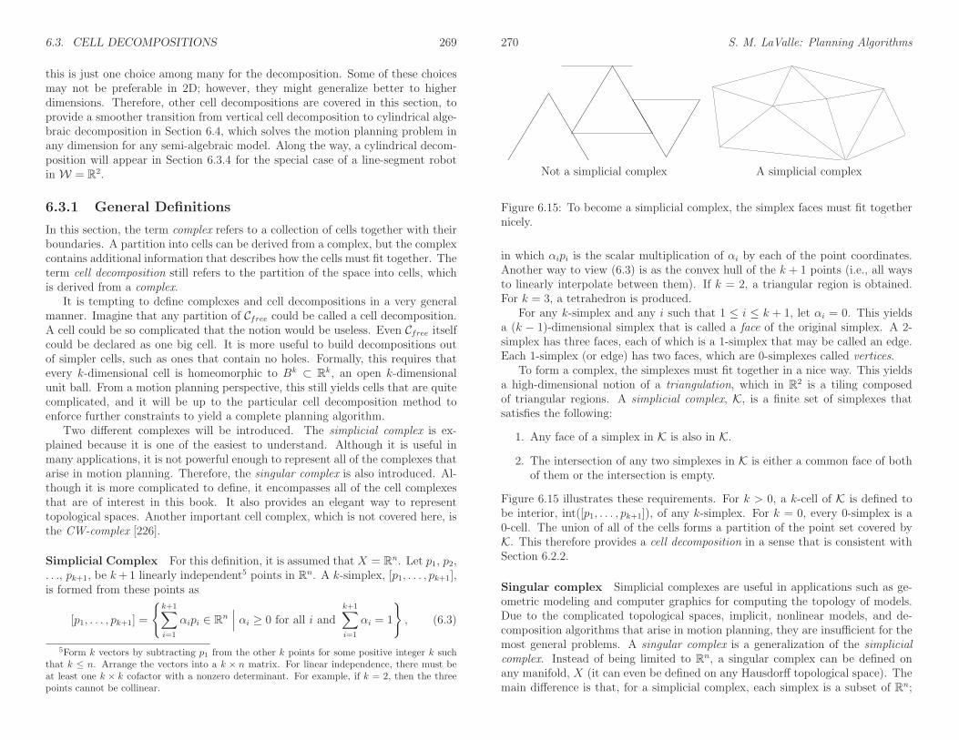
6.3. CELL DECOMPOSITIONS 269
this is just one choice among many for the decomposition. Some of these choicesmay not be preferable in 2D; however, they might generalize better to higherdimensions. Therefore, other cell decompositions are covered in this section, toprovide a smoother transition from vertical cell decomposition to cylindrical alge-braic decomposition in Section 6.4, which solves the motion planning problem inany dimension for any semi-algebraic model. Along the way, a cylindrical decom-position will appear in Section 6.3.4 for the special case of a line-segment robotin W = R2.
6.3.1 General Definitions
In this section, the term complex refers to a collection of cells together with theirboundaries. A partition into cells can be derived from a complex, but the complexcontains additional information that describes how the cells must fit together. Theterm cell decomposition still refers to the partition of the space into cells, whichis derived from a complex.
It is tempting to define complexes and cell decompositions in a very generalmanner. Imagine that any partition of Cfree could be called a cell decomposition.A cell could be so complicated that the notion would be useless. Even Cfree itselfcould be declared as one big cell. It is more useful to build decompositions outof simpler cells, such as ones that contain no holes. Formally, this requires thatevery k-dimensional cell is homeomorphic to Bk ⊂ Rk, an open k-dimensionalunit ball. From a motion planning perspective, this still yields cells that are quitecomplicated, and it will be up to the particular cell decomposition method toenforce further constraints to yield a complete planning algorithm.
Two different complexes will be introduced. The simplicial complex is ex-plained because it is one of the easiest to understand. Although it is useful inmany applications, it is not powerful enough to represent all of the complexes thatarise in motion planning. Therefore, the singular complex is also introduced. Al-though it is more complicated to define, it encompasses all of the cell complexesthat are of interest in this book. It also provides an elegant way to representtopological spaces. Another important cell complex, which is not covered here, isthe CW-complex [226].
Simplicial Complex For this definition, it is assumed that X = Rn. Let p1, p2,. . ., pk+1, be k+1 linearly independent5 points in Rn. A k-simplex, [p1, . . . , pk+1],is formed from these points as
[p1, . . . , pk+1] =
k+1∑
i=1
αipi ∈ Rn∣
∣
∣ αi ≥ 0 for all i andk+1∑
i=1
αi = 1
, (6.3)
5Form k vectors by subtracting p1 from the other k points for some positive integer k suchthat k ≤ n. Arrange the vectors into a k × n matrix. For linear independence, there must beat least one k × k cofactor with a nonzero determinant. For example, if k = 2, then the threepoints cannot be collinear.
270 S. M. LaValle: Planning Algorithms
Not a simplicial complex A simplicial complex
Figure 6.15: To become a simplicial complex, the simplex faces must fit togethernicely.
in which αipi is the scalar multiplication of αi by each of the point coordinates.Another way to view (6.3) is as the convex hull of the k + 1 points (i.e., all waysto linearly interpolate between them). If k = 2, a triangular region is obtained.For k = 3, a tetrahedron is produced.
For any k-simplex and any i such that 1 ≤ i ≤ k + 1, let αi = 0. This yieldsa (k − 1)-dimensional simplex that is called a face of the original simplex. A 2-simplex has three faces, each of which is a 1-simplex that may be called an edge.Each 1-simplex (or edge) has two faces, which are 0-simplexes called vertices.
To form a complex, the simplexes must fit together in a nice way. This yieldsa high-dimensional notion of a triangulation, which in R2 is a tiling composedof triangular regions. A simplicial complex, K, is a finite set of simplexes thatsatisfies the following:
1. Any face of a simplex in K is also in K.
2. The intersection of any two simplexes in K is either a common face of bothof them or the intersection is empty.
Figure 6.15 illustrates these requirements. For k > 0, a k-cell of K is defined tobe interior, int([p1, . . . , pk+1]), of any k-simplex. For k = 0, every 0-simplex is a0-cell. The union of all of the cells forms a partition of the point set covered byK. This therefore provides a cell decomposition in a sense that is consistent withSection 6.2.2.
Singular complex Simplicial complexes are useful in applications such as ge-ometric modeling and computer graphics for computing the topology of models.Due to the complicated topological spaces, implicit, nonlinear models, and de-composition algorithms that arise in motion planning, they are insufficient for themost general problems. A singular complex is a generalization of the simplicialcomplex. Instead of being limited to Rn, a singular complex can be defined onany manifold, X (it can even be defined on any Hausdorff topological space). Themain difference is that, for a simplicial complex, each simplex is a subset of Rn;

6.3. CELL DECOMPOSITIONS 271
however, for a singular complex, each singular simplex is actually a homeomor-phism from a (simplicial) simplex in Rn to a subset of X.
To help understand the idea, first consider a 1D singular complex, which hap-pens to be a topological graph (as introduced in Example 4.6). The interval [0, 1]is a 1-simplex, and a continuous path τ : [0, 1] → X is a singular 1-simplex be-cause it is a homeomorphism of [0, 1] to the image of τ in X. Suppose G(V,E) isa topological graph. The cells are subsets of X that are defined as follows. Eachpoint v ∈ V is a 0-cell in X. To follow the formalism, each is considered as theimage of a function f : 0 → X, which makes it a singular 0-simplex, because0 is a 0-simplex. For each path τ ∈ E, the corresponding 1-cell is
x ∈ X | τ(s) = x for some s ∈ (0, 1). (6.4)
Expressed differently, it is τ((0, 1)), the image of the path τ , except that theendpoints are removed because they are already covered by the 0-cells (the cellsmust form a partition).
These principles will now be generalized to higher dimensions. Since all ballsand simplexes of the same dimension are homeomorphic, balls can be used insteadof a simplex in the definition of a singular simplex. Let Bk ⊂ Rk denote a closed,k-dimensional unit ball,
Dk = x ∈ Rn | ‖x‖ ≤ 1, (6.5)
in which ‖·‖ is the Euclidean norm. A singular k-simplex is a continuous mappingσ : Dk → X. Let int(Dk) refer to the interior of Dk. For k ≥ 1, the k-cell, C,corresponding to a singular k-simplex, σ, is the image C = σ(int(Dk)) ⊆ X.The 0-cells are obtained directly as the images of the 0 singular simplexes. Eachsingular 0-simplex maps to the 0-cell in X. If σ is restricted to int(Dk), then itactually defines a homeomorphism between Dk and C. Note that both of theseare open sets if k > 0.
A simplicial complex requires that the simplexes fit together nicely. The sameconcept is applied here, but topological concepts are used instead because theyare more general. Let K be a set of singular simplexes of varying dimensions. LetSk denote the union of the images of all singular i-simplexes for all i ≤ k.
A collection of singular simplexes that map into a topological space X is calleda singular complex if:
1. For each dimension k, the set Sk ⊆ X must be closed. This means that thecells must all fit together nicely.
2. Each k-cell is an open set in the topological subspace Sk. Note that 0-cellsare open in S0, even though they are usually closed in X.
Example 6.1 (Vertical Decomposition) The vertical decomposition of Sec-tion 6.2.2 is a nice example of a singular complex that is not a simplicial complex
272 S. M. LaValle: Planning Algorithms
because it contains trapezoids. The interior of each trapezoid and triangle formsa 2-cell, which is an open set. For every pair of adjacent 2-cells, there is a 1-cell ontheir common boundary. There are no 0-cells because the vertices lie in Cobs, notin Cfree. The subspace S2 is formed by taking the union of all 2-cells and 1-cellsto yield S2 = Cfree. This satisfies the closure requirement because the complexis built in Cfree only; hence, the topological space is Cfree. The set S2 = Cfree isboth open and closed. The set S1 is the union of all 1-cells. This is also closedbecause the 1-cell endpoints all lie in Cobs. Each 1-cell is also an open set.
One way to avoid some of these strange conclusions from the topology re-stricted to Cfree is to build the vertical decomposition in cl(Cfree), the closure ofCfree. This can be obtained by starting with the previously defined vertical de-composition and adding a new 1-cell for every edge of Cobs and a 0-cell for everyvertex of Cobs. Now S3 = cl(Cfree), which is closed in R2. Likewise, S2, S1, and S0,are closed in the usual way. Each of the individual k-dimensional cells, however,is open in the topological space Sk. The only strange case is that the 0-cells areconsidered open, but this is true in the discrete topological space S0.
6.3.2 2D Decompositions
The vertical decomposition method of Section 6.2.2 is just one choice of manycell decomposition methods for solving the problem when Cobs is polygonal. Itprovides a nice balance between the number of cells, computational efficiency,and implementation ease. It is usually possible to decompose Cobs into far fewerconvex cells. This would be preferable for multiple-query applications becausethe roadmap would be smaller. It is unfortunately quite difficult to optimize thenumber of cells. Determining the decomposition of a polygonal Cobs with holesthat uses the smallest number of convex cells is NP-hard [268, 336]. Therefore,we are willing to tolerate nonoptimal decompositions.
Triangulation One alternative to the vertical decomposition is to perform atriangulation, which yields a simplicial complex over Cfree. Figure 6.16 shows anexample. Since Cfree is an open set, there are no 0-cells. Each 2-simplex (triangle)has either one, two, or three faces, depending on how much of its boundary isshared with Cobs. A roadmap can be made by connecting the samples for 1-cellsand 2-cells as shown in Figure 6.17. Note that there are many ways to triangulateCfree for a given problem. Finding good triangulations, which for example meanstrying to avoid thin triangles, is given considerable attention in computationalgeometry [71, 146, 158].
How can the triangulation be computed? It might seem tempting to run thevertical decomposition algorithm of Section 6.2.2 and split each trapezoid intotwo triangles. Even though this leads to triangular cells, it does not produce asimplicial complex (two triangles could abut the same side of a triangle edge).

6.3. CELL DECOMPOSITIONS 273
Figure 6.16: A triangulation of Cfree.
Figure 6.17: A roadmap obtained from the triangulation.
274 S. M. LaValle: Planning Algorithms
A naive approach is to incrementally split faces by attempting to connect twovertices of a face by a line segment. If this segment does not intersect othersegments, then the split can be made. This process can be iteratively performedover all vertices of faces that have more than three vertices, until a triangulationis eventually obtained. Unfortunately, this results in an O(n3) time algorithmbecause O(n2) pairs must be checked in the worst case, and each check requiresO(n) time to determine whether an intersection occurs with other segments. Thiscan be easily reduced to O(n2 lg n) by performing radial sweeping. Chapter 3of [146] presents an algorithm that runs in O(n lg n) time by first partitioningCfree into monotone polygons, and then efficiently triangulating each monotonepolygon. If Cfree is simply connected, then, surprisingly, a triangulation can becomputed in linear time [104]. Unfortunately, this algorithm is too complicated touse in practice (there are, however, simpler algorithms for which the complexityis close to O(n); see [57] and the end of Chapter 3 of [146] for surveys).
Cylindrical decomposition The cylindrical decomposition is very similar tothe vertical decomposition, except that when any of the cases in Figure 6.2 occurs,then a vertical line slices through all faces, all the way from y = −∞ to y = ∞.The result is shown in Figure 6.18, which may be considered as a singular complex.This may appear very inefficient in comparison to the vertical decomposition;however, it is presented here because it generalizes nicely to any dimension, anyC-space topology, and any semi-algebraic model. Therefore, it is presented here toease the transition to more general decompositions. The most important propertyof the cylindrical decomposition is shown in Figure 6.19. Consider each verticalstrip between two events. When traversing a strip from y = −∞ to y = ∞,the points alternate between being Cobs and Cfree. For example, between events4 and 5, the points below edge f are in Cfree. Points between f and g lie inCobs. Points between g and h lie in Cfree, and so forth. The cell decompositioncan be defined so that 2D cells are also created in Cobs. Let S(x, y) denote thelogical predicate (3.6) from Section 3.1.1. When traversing a strip, the value ofS(x, y) also alternates. This behavior is the main reason to construct a cylindricaldecomposition, which will become clearer in Section 6.4.2. Each vertical strip isactually considered to be a cylinder, hence, the name cylindrical decomposition(i.e., there are not necessarily any cylinders in the 3D geometric sense).
6.3.3 3D Vertical Decomposition
It turns out that the vertical decomposition method of Section 6.2.2 can be ex-tended to any dimension by recursively applying the sweeping idea. The methodrequires, however, that Cobs is piecewise linear. In other words, Cobs is representedas a semi-algebraic model for which all primitives are linear. Unfortunately, mostof the general motion planning problems involve nonlinear algebraic primitivesbecause of the nonlinear transformations that arise from rotations. Recall the

6.3. CELL DECOMPOSITIONS 275
1 2 3 4 5 6 7 8 9 10 11 12 130
a
b
i
h
gc
e
l
f
j
k
nm
d
Figure 6.18: The cylindrical decomposition differs from the vertical decompositionin that the rays continue forever instead of stopping at the nearest edge. Comparethis figure to Figure 6.6.
1 2 3 4 5 6 7 8 9 10 11 12 130
a
b
i
h
gc
e
l
mn
d
k
f
j
Figure 6.19: The cylindrical decomposition produces vertical strips. Inside of astrip, there is a stack of collision-free cells, separated by Cobs.
276 S. M. LaValle: Planning Algorithms
y y y
z z z
y
z
x
Figure 6.20: In higher dimensions, the sweeping idea can be applied recursively.
complicated algebraic Cobs model constructed in Section 4.3.3. To handle genericalgebraic models, powerful techniques from computational algebraic geometry areneeded. This will be covered in Section 6.4.
One problem for which Cobs is piecewise linear is a polyhedral robot that cantranslate in R3, and the obstacles in W are polyhedra. Since the transformationequations are linear in this case, Cobs ⊂ R3 is polyhedral. The polygonal faces ofCobs are obtained by forming geometric primitives for each of the Type FV, TypeVF, and Type EE cases of contact between A and O, as mentioned in Section4.3.2.
Figure 6.20 illustrates the algorithm that constructs the 3D vertical decompo-sition. Compare this to the algorithm in Section 6.2.2. Let (x, y, z) denote a pointin C = R3. The vertical decomposition yields convex 3-cells, 2-cells, and 1-cells.Neglecting degeneracies, a generic 3-cell is bounded by six planes. The cross sec-tion of a 3-cell for some fixed x value yields a trapezoid or triangle, exactly as inthe 2D case, but in a plane parallel to the yz plane. Two sides of a generic 3-cellare parallel to the yz plane, and two other sides are parallel to the xz plane. The3-cell is bounded above and below by two polygonal faces of Cobs.

6.3. CELL DECOMPOSITIONS 277
Initially, sort the Cobs vertices by their x coordinate to obtain the events. Nowconsider sweeping a plane perpendicular to the x-axis. The plane for a fixed valueof x produces a 2D polygonal slice of Cobs. Three such slices are shown at thebottom of Figure 6.20. Each slice is parallel to the yz plane and appears to lookexactly like a problem that can be solved by the 2D vertical decomposition method.The 2-cells in a slice are actually slices of 3-cells in the 3D decomposition. Theonly places in which these 3-cells can critically change is when the sweeping planestops at some x value. The center slice in Figure 6.20 corresponds to the case inwhich a vertex of a convex polyhedron is encountered, and all of the polyhedronlies to right of the sweep plane (i.e., the rest of the polyhedron has not beenencountered yet). This corresponds to a place where a critical change must occurin the slices. These are 3D versions of the cases in Figure 6.2, which indicate howthe vertical decomposition needs to be updated. The algorithm proceeds by firstbuilding the 2D vertical decomposition at the first x event. At each event, the 2Dvertical decomposition must be updated to take into account the critical changes.During this process, the 3D cell decomposition and roadmap can be incrementallyconstructed, as in the 2D case.
The roadmap is constructed by placing a sample point in the center of each3-cell and 2-cell. The vertices are the sample points, and edges are added tothe roadmap by connecting the sample points for each case in which a 3-cell isadjacent to a 2-cell.
This same principle can be extended to any dimension, but the applications tomotion planning are limited because the method requires linear models (or at leastit is very challenging to adapt to nonlinear models; in some special cases, this canbe done). See [216] for a summary of the complexity of vertical decompositionsfor various geometric primitives and dimensions.
6.3.4 A Decomposition for a Line-Segment Robot
This section presents one of the simplest cell decompositions that involves non-linear models, yet it is already fairly complicated. This will help to give anappreciation of the difficulty of combinatorial planning in general. Consider theplanning problem shown in Figure 6.21. The robot, A, is a single line segmentthat can translate or rotate in W = R2. The dot on one end of A is used to illus-trate its origin and is not part of the model. The C-space, C, is homeomorphic toR2 × S1. Assume that the parameterization R2 × [0, 2π]/ ∼ is used in which theidentification equates θ = 0 and θ = 2π. A point in C is represented as (x, y, θ).
An approximate solution First consider making a cell decomposition for thecase in which the segment can only translate. The method from Section 4.3.2 canbe used to compute Cobs by treating the robot-obstacle interaction with Type EVand Type VE contacts. When the interior of A touches an obstacle vertex, thenType EV is obtained. An endpoint of A touching an object interior yields Type
278 S. M. LaValle: Planning Algorithms
Figure 6.21: Motion planning for a line segment that can translate and rotate ina 2D world.
VE. Each case produces an edge of Cobs, which is polygonal. Once this is repre-sented, the vertical decomposition can be used to solve the problem. This inspiresa reasonable numerical approach to the rotational case, which is to discretize θinto K values, i∆θ, for 0 ≤ i ≤ K, and ∆θ = 2π/K [14]. The obstacle region,Cobs, is polygonal for each case, and we can imagine having a stack of K polyg-onal regions. A roadmap can be formed by connecting sampling points inside ofa slice in the usual way, and also by connecting samples between correspondingcells in neighboring slices. If K is large enough, this strategy works well, but themethod is not complete because a sufficient value for K cannot be determined inadvance. The method is actually an interesting hybrid between combinatorial andsampling-based motion planning. A resolution-complete version can be imagined.
In the limiting case, as K tends to infinity, the surfaces of Cobs become curvedalong the θ direction. The conditions in Section 4.3.3 must be applied to gen-erate the actual obstacle regions. This is possible, but it yields a semi-algebraicrepresentation of Cobs in terms of implicit polynomial primitives. It is no easytask to determine an explicit representation in terms of simple cells that can beused for motion planning. The method of Section 6.3.3 cannot be used becauseCobs is not polyhedral. Therefore, special analysis is warranted to produce a celldecomposition.
The general idea is to construct a cell decomposition in R2 by considering onlythe translation part, (x, y). Each cell in R2 is then lifted into C by considering θ asa third axis that is “above” the xy plane. A cylindrical decomposition results inwhich each cell in the xy plane produces a cylindrical stack of cells for different θvalues. Recall the cylinders in Figures 6.18 and 6.19. The vertical axis correspondsto θ in the current setting, and the horizontal axis is replaced by two axes, x andy.
To construct the decomposition in R2, consider the various robot-obstacle con-tacts shown in Figure 6.22. In Figure 6.22a, the segment swings around from afixed (x, y). Two different kinds of contacts arise. For some orientation (value of

6.3. CELL DECOMPOSITIONS 279
v1
e3
e2
e1
v1
e3e3
e2
(a) (b)
Figure 6.22: Fix (x, y) and swing the segment around for all values of θ ∈[0, 2π]/ ∼. (a) Note the vertex and edge features that are hit by the segment.(b) Record orientation intervals over which the robot is not in collision.
θ), the segment contacts v1, forming a Type EV contact. For three other orienta-tions, the segment contacts an edge, forming Type VE contacts. Once again usingthe feature concept, there are four orientations at which the segment contacts afeature. Each feature may be either a vertex or an edge. Between the two contactswith e2 and e3, the robot is not in collision. These configurations lie in Cfree. Also,configurations for which the robot is between contacts e3 (the rightmost contact)and v1 are also in Cfree. All other orientations produce configurations in Cobs. Notethat the line segment cannot get from being between e2 and e3 to being betweene3 and v1, unless the (x, y) position is changed. It therefore seems sensible thatthese must correspond to different cells in whatever decomposition is made.
Radar maps Figure 6.22b illustrates which values of θ produce collision. Wewill refer to this representation as a radar map. The four contact orientations areindicated by the contact feature. The notation [e3, v1] and [e2, e3] identifies thetwo intervals for which (x, y, θ) ∈ Cfree. Now imagine changing (x, y) by a smallamount, to obtain (x′, y′). How would the radar map change? The precise anglesat which the contacts occur would change, but the notation [e3, v1] and [e2, e3],for configurations that lie in Cfree, remains unchanged. Even though the angleschange, there is no interesting change in terms of the contacts; therefore, it makessense to declare (x, y, θ) and (x, y, θ′) to lie in the same cell in Cfree because θ andθ′ both place the segment between the same contacts. Imagine a column of two3-cells above a small area around (x, y). One 3-cell is for orientations in [e3, v1],and the other is for orientations in [e2, e3]. These appear to be 3D regions in Cfreebecause each of x, y, and θ can be perturbed a small amount without leaving thecell.
Of course, if (x, y) is changed enough, then eventually we expect a dramaticchange to occur in the radar map. For example, imagine e3 is infinitely long, andthe x value is gradually increased in Figure 6.22a. The black band between v1 and
280 S. M. LaValle: Planning Algorithms
e2
e1
e3
v1
e3e3
(a) (b)
Figure 6.23: If x is increased enough, a critical change occurs in the radar mapbecause v1 can no longer be reached by the robot.
e2 in Figure 6.22b shrinks in length. Eventually, when the distance from (x′, y′)to v1 is greater than the length of A, the black band disappears. This situationis shown in Figure 6.23. The change is very important to notice because afterthat region vanishes, any orientation θ′ between e3 and e3, traveling the long wayaround the circle, produces a configuration (x′, y′, θ′) ∈ Cfree. This seems veryimportant because it tells us that we can travel between the original two cells bymoving the robot further way from v1, rotating the robot, and then moving back.Now move from the position shown in Figure 6.23 into the positive y direction. Theremaining black band begins to shrink and finally disappears when the distanceto e3 is further than the robot length. This represents another critical change.
The radar map can be characterized by specifying a circular ordering
([f1, f2], [f3, f4], [f5, f6], . . . , [f2k−1, f2k]), (6.6)
when there are k orientation intervals over which the configurations lie in Cfree.For the radar map in Figure 6.22b, this representation yields ([e3, v1], [e2, e3]).Each fi is a feature, which may be an edge or a vertex. Some of the fi maybe identical; the representation for Figure 6.23b is ([e3, e3]). The intervals arespecified in counterclockwise order around the radar map. Since the orderingis circular, it does not matter which interval is specified first. There are twodegenerate cases. If (x, y, θ) ∈ Cfree for all θ ∈ [0, 2π), then we write () for theordering. On the other hand, if (x, y, θ) ∈ Cobs for all θ ∈ [0, 2π), then we write ∅.
Critical changes in cells Now we are prepared to explain the cell decompo-sition in more detail. Imagine traveling along a path in R2 and producing ananimated version of the radar map in Figure 6.22b. We say that a critical changeoccurs each time the circular ordering representation of (6.6) changes. Changesoccur when intervals: 1) appear, 2) disappear, 3) split apart, 4) merge into one,or 5) when the feature of an interval changes. The first task is to partition R2 into

6.3. CELL DECOMPOSITIONS 281
e
L
v
L
(a) (b)
ev
L
Lv1
v2
(c) (d)
Figure 6.24: Four of the five cases that produce critical curves in R2.
maximal 2-cells over which no critical changes occur. Each one of these 2-cells,R, represents the projection of a strip of 3-cells in Cfree. Each 3-cell is defined asfollows. Let R, [fi, fi+1] denote the 3D region in Cfree for which (x, y) ∈ R andθ places the segment between contacts fi and fi+1. The cylinder of cells above Ris given by R, [fi, fi+1] for each interval in the circular ordering representation,(6.6). If any orientation is possible because A never contacts an obstacle while inR, then we write R.
What are the positions in R2 that cause critical changes to occur? It turnsout that there are five different cases to consider, each of which produces a set ofcritical curves in R2. When one of these curves is crossed, a critical change occurs.If none of these curves is crossed, then no critical change can occur. Therefore,these curves precisely define the boundaries of the desired 2-cells in R2. Let Ldenote the length of the robot (which is the line segment).
Consider how the five cases mentioned above may occur. Two of the five caseshave already been observed in Figures 6.22 and 6.23. These appear in Figures6.24a and Figures 6.24b, and occur if (x, y) is within L of an edge or a vertex.The third and fourth cases are shown in Figures 6.24c and 6.24d, respectively. Thethird case occurs because crossing the curve causes A to change between beingable to touch e and being able to touch v. This must be extended from any edgeat an endpoint that is a reflex vertex (interior angle is greater than π). The fourthcase is actually a return of the bitangent case from Figure 6.10, which arose for
282 S. M. LaValle: Planning Algorithms
v
eA
L
Figure 6.25: The fifth case is the most complicated. It results in a fourth-degreealgebraic curve called the Conchoid of Nicomedes.
R1 R2 R3 R4
R6R7
R9
R10
R11
R12
R13
A
R8
R5
e3
e2
x2
x1
e4
e1
Figure 6.26: The critical curves form the boundaries of the noncritical regions inR2.
the shortest path graph. If the vertices are within L of each other, then a linearcritical curve is generated because A is no longer able to touch v2 when crossing itfrom right to left. Bitangents always produce curves in pairs; the curve above v2is not shown. The final case, shown in Figure 6.25, is the most complicated. It is afourth-degree algebraic curve called the Conchoid of Nicomedes, which arises fromA being in simultaneous contact between v and e. Inside of the teardrop-shapedcurve, A can contact e but not v. Just outside of the curve, it can touch v. If thexy coordinate frame is placed so that v is at (0, 0), then the equation of the curveis
(x2 − y2)(y + d)2 − y2L2 = 0, (6.7)
in which d is the distance from v to e.Putting all of the curves together generates a cell decomposition of R2. There
are noncritical regions, over which there is no change in (6.6); these form the2-cells. The boundaries between adjacent 2-cells are sections of the critical curvesand form 1-cells. There are also 0-cells at places where critical curves intersect.
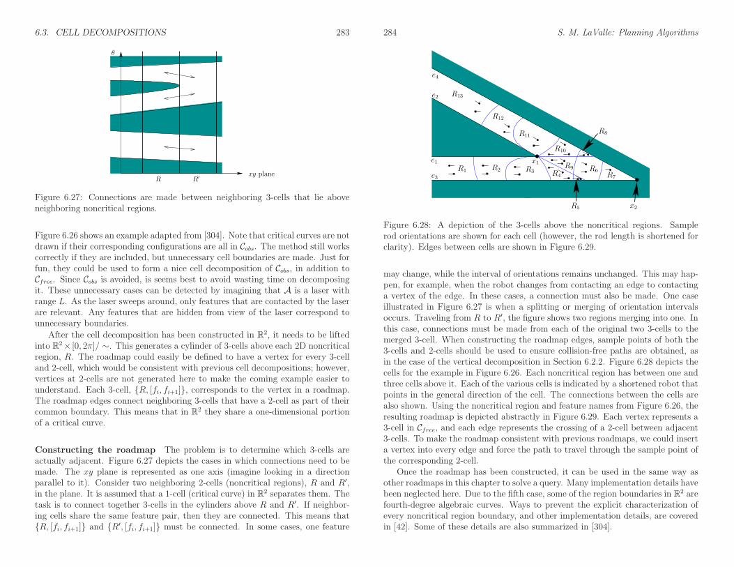
6.3. CELL DECOMPOSITIONS 283
xy planeR R′
θ
Figure 6.27: Connections are made between neighboring 3-cells that lie aboveneighboring noncritical regions.
Figure 6.26 shows an example adapted from [304]. Note that critical curves are notdrawn if their corresponding configurations are all in Cobs. The method still workscorrectly if they are included, but unnecessary cell boundaries are made. Just forfun, they could be used to form a nice cell decomposition of Cobs, in addition toCfree. Since Cobs is avoided, is seems best to avoid wasting time on decomposingit. These unnecessary cases can be detected by imagining that A is a laser withrange L. As the laser sweeps around, only features that are contacted by the laserare relevant. Any features that are hidden from view of the laser correspond tounnecessary boundaries.
After the cell decomposition has been constructed in R2, it needs to be liftedinto R2× [0, 2π]/ ∼. This generates a cylinder of 3-cells above each 2D noncriticalregion, R. The roadmap could easily be defined to have a vertex for every 3-celland 2-cell, which would be consistent with previous cell decompositions; however,vertices at 2-cells are not generated here to make the coming example easier tounderstand. Each 3-cell, R, [fi, fi+1], corresponds to the vertex in a roadmap.The roadmap edges connect neighboring 3-cells that have a 2-cell as part of theircommon boundary. This means that in R2 they share a one-dimensional portionof a critical curve.
Constructing the roadmap The problem is to determine which 3-cells areactually adjacent. Figure 6.27 depicts the cases in which connections need to bemade. The xy plane is represented as one axis (imagine looking in a directionparallel to it). Consider two neighboring 2-cells (noncritical regions), R and R′,in the plane. It is assumed that a 1-cell (critical curve) in R2 separates them. Thetask is to connect together 3-cells in the cylinders above R and R′. If neighbor-ing cells share the same feature pair, then they are connected. This means thatR, [fi, fi+1] and R′, [fi, fi+1] must be connected. In some cases, one feature
284 S. M. LaValle: Planning Algorithms
R7
R5
e3
e2
x2
x1
e4
e1
R10
R9
R8
R13
R11
R12
R2 R3R1 R6R4
Figure 6.28: A depiction of the 3-cells above the noncritical regions. Samplerod orientations are shown for each cell (however, the rod length is shortened forclarity). Edges between cells are shown in Figure 6.29.
may change, while the interval of orientations remains unchanged. This may hap-pen, for example, when the robot changes from contacting an edge to contactinga vertex of the edge. In these cases, a connection must also be made. One caseillustrated in Figure 6.27 is when a splitting or merging of orientation intervalsoccurs. Traveling from R to R′, the figure shows two regions merging into one. Inthis case, connections must be made from each of the original two 3-cells to themerged 3-cell. When constructing the roadmap edges, sample points of both the3-cells and 2-cells should be used to ensure collision-free paths are obtained, asin the case of the vertical decomposition in Section 6.2.2. Figure 6.28 depicts thecells for the example in Figure 6.26. Each noncritical region has between one andthree cells above it. Each of the various cells is indicated by a shortened robot thatpoints in the general direction of the cell. The connections between the cells arealso shown. Using the noncritical region and feature names from Figure 6.26, theresulting roadmap is depicted abstractly in Figure 6.29. Each vertex represents a3-cell in Cfree, and each edge represents the crossing of a 2-cell between adjacent3-cells. To make the roadmap consistent with previous roadmaps, we could inserta vertex into every edge and force the path to travel through the sample point ofthe corresponding 2-cell.
Once the roadmap has been constructed, it can be used in the same way asother roadmaps in this chapter to solve a query. Many implementation details havebeen neglected here. Due to the fifth case, some of the region boundaries in R2 arefourth-degree algebraic curves. Ways to prevent the explicit characterization ofevery noncritical region boundary, and other implementation details, are coveredin [42]. Some of these details are also summarized in [304].
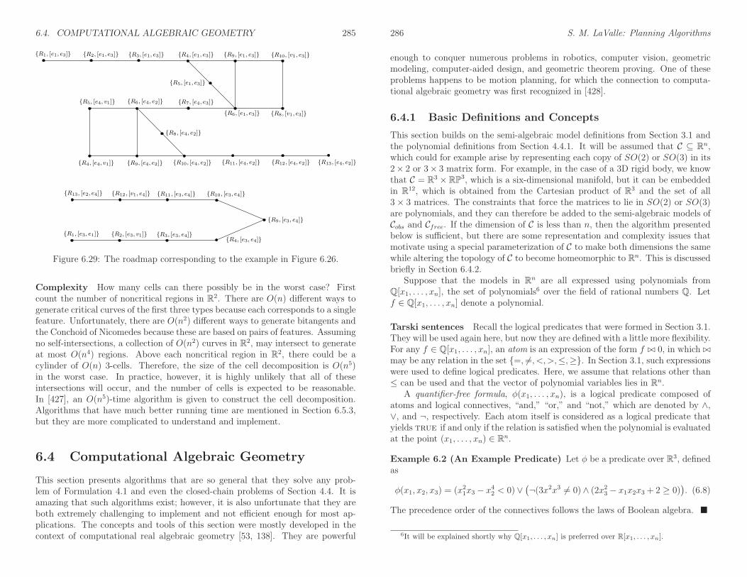
6.4. COMPUTATIONAL ALGEBRAIC GEOMETRY 285
R1, [e1, e3] R2, [e1, e3] R3, [e1, e3] R4, [e1, e3] R9, [e1, e3] R10, [v1, e3]
R5, [e1, e3]
R8, [v1, e3]R6, [e1, e3]
R7, [e4, e3]R6, [e4, e2]R5, [e4, v1]
R8, [e4, e2]
R4, [e4, v1] R9, [e4, e2] R10, [e4, e2] R11, [e4, e2] R12, [e4, e2] R13, [e4, e2]
R1, [e3, e1] R2, [e3, v1] R3, [e3, e4]
R9, [e3, e4]
R10, [e3, e4]R11, [e3, e4]R12, [v1, e4]R13, [e2, e4]
R4, [e3, e4]
Figure 6.29: The roadmap corresponding to the example in Figure 6.26.
Complexity How many cells can there possibly be in the worst case? Firstcount the number of noncritical regions in R2. There are O(n) different ways togenerate critical curves of the first three types because each corresponds to a singlefeature. Unfortunately, there are O(n2) different ways to generate bitangents andthe Conchoid of Nicomedes because these are based on pairs of features. Assumingno self-intersections, a collection of O(n2) curves in R2, may intersect to generateat most O(n4) regions. Above each noncritical region in R2, there could be acylinder of O(n) 3-cells. Therefore, the size of the cell decomposition is O(n5)in the worst case. In practice, however, it is highly unlikely that all of theseintersections will occur, and the number of cells is expected to be reasonable.In [427], an O(n5)-time algorithm is given to construct the cell decomposition.Algorithms that have much better running time are mentioned in Section 6.5.3,but they are more complicated to understand and implement.
6.4 Computational Algebraic Geometry
This section presents algorithms that are so general that they solve any prob-lem of Formulation 4.1 and even the closed-chain problems of Section 4.4. It isamazing that such algorithms exist; however, it is also unfortunate that they areboth extremely challenging to implement and not efficient enough for most ap-plications. The concepts and tools of this section were mostly developed in thecontext of computational real algebraic geometry [53, 138]. They are powerful
286 S. M. LaValle: Planning Algorithms
enough to conquer numerous problems in robotics, computer vision, geometricmodeling, computer-aided design, and geometric theorem proving. One of theseproblems happens to be motion planning, for which the connection to computa-tional algebraic geometry was first recognized in [428].
6.4.1 Basic Definitions and Concepts
This section builds on the semi-algebraic model definitions from Section 3.1 andthe polynomial definitions from Section 4.4.1. It will be assumed that C ⊆ Rn,which could for example arise by representing each copy of SO(2) or SO(3) in its2× 2 or 3× 3 matrix form. For example, in the case of a 3D rigid body, we knowthat C = R3 ×RP3, which is a six-dimensional manifold, but it can be embeddedin R12, which is obtained from the Cartesian product of R3 and the set of all3× 3 matrices. The constraints that force the matrices to lie in SO(2) or SO(3)are polynomials, and they can therefore be added to the semi-algebraic models ofCobs and Cfree. If the dimension of C is less than n, then the algorithm presentedbelow is sufficient, but there are some representation and complexity issues thatmotivate using a special parameterization of C to make both dimensions the samewhile altering the topology of C to become homeomorphic to Rn. This is discussedbriefly in Section 6.4.2.
Suppose that the models in Rn are all expressed using polynomials fromQ[x1, . . . , xn], the set of polynomials6 over the field of rational numbers Q. Letf ∈ Q[x1, . . . , xn] denote a polynomial.
Tarski sentences Recall the logical predicates that were formed in Section 3.1.They will be used again here, but now they are defined with a little more flexibility.For any f ∈ Q[x1, . . . , xn], an atom is an expression of the form f ⊲⊳ 0, in which ⊲⊳may be any relation in the set =, 6=, <,>,≤,≥. In Section 3.1, such expressionswere used to define logical predicates. Here, we assume that relations other than≤ can be used and that the vector of polynomial variables lies in Rn.
A quantifier-free formula, φ(x1, . . . , xn), is a logical predicate composed ofatoms and logical connectives, “and,” “or,” and “not,” which are denoted by ∧,∨, and ¬, respectively. Each atom itself is considered as a logical predicate thatyields true if and only if the relation is satisfied when the polynomial is evaluatedat the point (x1, . . . , xn) ∈ Rn.
Example 6.2 (An Example Predicate) Let φ be a predicate over R3, definedas
φ(x1, x2, x3) = (x21x3 − x42 < 0)∨(
¬(3x2x3 6= 0)∧ (2x23 − x1x2x3 + 2 ≥ 0))
. (6.8)
The precedence order of the connectives follows the laws of Boolean algebra.
6It will be explained shortly why Q[x1, . . . , xn] is preferred over R[x1, . . . , xn].
6.4. COMPUTATIONAL ALGEBRAIC GEOMETRY 287
Let a quantifier Q be either of the symbols, ∀, which means “for all,” or ∃,which means “there exists.” A Tarski sentence Φ is a logical predicate that mayadditionally involve quantifiers on some or all of the variables. In general, a Tarskisentence takes the form
Φ(x1, . . . , xn−k) = (Qz1)(Qz2) . . . (Qzk) φ(z1, . . . , zk, x1, . . . , xn−k), (6.9)
in which the zi are the quantified variables, the xi are the free variables, and φ isa quantifier-free formula. The quantifiers do not necessarily have to appear at theleft to be a valid Tarski sentence; however, any expression can be manipulatedinto an equivalent expression that has all quantifiers in front, as shown in (6.9).The procedure for moving quantifiers to the front is as follows [370]: 1) Eliminateany redundant quantifiers; 2) rename some of the variables to ensure that thesame variable does not appear both free and bound; 3) move negation symbols asfar inward as possible; and 4) push the quantifiers to the left.
Example 6.3 (Several Tarski Sentences) Tarski sentences that have no freevariables are either true or false in general because there are no arguments onwhich the results depend. The sentence
Φ = ∀x∃y (x2 − y < 0), (6.10)
is true because for any x ∈ R, some y ∈ R can always be chosen so that y > x2.In the general notation of (6.9), this example becomes Qz1 = ∀x, Qz2 = ∃y, andφ(z1, z2) = (x2 − y < 0).
Swapping the order of the quantifiers yields the Tarski sentence
Φ = ∃y∀x (x2 − y < 0), (6.11)
which is false because for any y, there is always an x such that x2 > y.Now consider a Tarski sentence that has a free variable:
Φ(z) = ∃y∀x (x2 − zx2 − y < 0). (6.12)
This yields a function Φ : R→ true, false, in which
Φ(z) =
true if z ≥ 1false if z < 1.
(6.13)
An equivalent quantifier-free formula φ can be defined as φ(z) = (z > 1), whichtakes on the same truth values as the Tarski sentence in (6.12). This might makeyou wonder whether it is always possible to make a simplification that eliminatesthe quantifiers. This is called the quantifier-elimination problem, which will beexplained shortly.
288 S. M. LaValle: Planning Algorithms
The decision problem The sentences in (6.10) and (6.11) lead to an interestingproblem. Consider the set of all Tarski sentences that have no free variables. Thesubset of these that are true comprise the first-order theory of the reals. Canan algorithm be developed to determine whether such a sentence is true? Thisis called the decision problem for the first-order theory of the reals. At firstit may appear hopeless because Rn is uncountably infinite, and an algorithmmust work with a finite set. This is a familiar issue faced throughout motionplanning. The sampling-based approaches in Chapter 5 provided one kind ofsolution. This idea could be applied to the decision problem, but the resultinglack of completeness would be similar. It is not possible to check all possible pointsin Rn by sampling. Instead, the decision problem can be solved by constructinga combinatorial representation that exactly represents the decision problem bypartitioning Rn into a finite collection of regions. Inside of each region, only onepoint needs to be checked. This should already seem related to cell decompositionsin motion planning; it turns out that methods developed to solve the decisionproblem can also conquer motion planning.
The quantifier-elimination problem Another important problem was exem-plified in (6.12). Consider the set of all Tarski sentences of the form (6.9), whichmay or may not have free variables. Can an algorithm be developed that takesa Tarski sentence Φ and produces an equivalent quantifier-free formula φ? Letx1, . . . , xn denote the free variables. To be equivalent, both must take on thesame true values over Rn, which is the set of all assignments (x1, . . . , xn) for thefree variables.
Given a Tarski sentence, (6.9), the quantifier-elimination problem is to find aquantifier-free formula φ such that
Φ(x1, . . . , xn) = φ(x1, . . . , xn) (6.14)
for all (x1, . . . , xn) ∈ Rn. This is equivalent to constructing a semi-algebraic modelbecause φ can always be expressed in the form
φ(x1, . . . , xn) =k∨
i=1
mi∧
j=1
(fi,j(x1, . . . , xn) ⊲⊳ 0) , (6.15)
in which ⊲⊳ may be either <, =, or >. This appears to be the same (3.6), exceptthat (6.15) uses the relations <, =, and > to allow open and closed semi-algebraicsets, whereas (3.6) only used ≤ to construct closed semi-algebraic sets for O andA.
Once again, the problem is defined on Rn, which is uncountably infinite, butan algorithm must work with a finite representation. This will be achieved by thecell decomposition technique presented in Section 6.4.2.
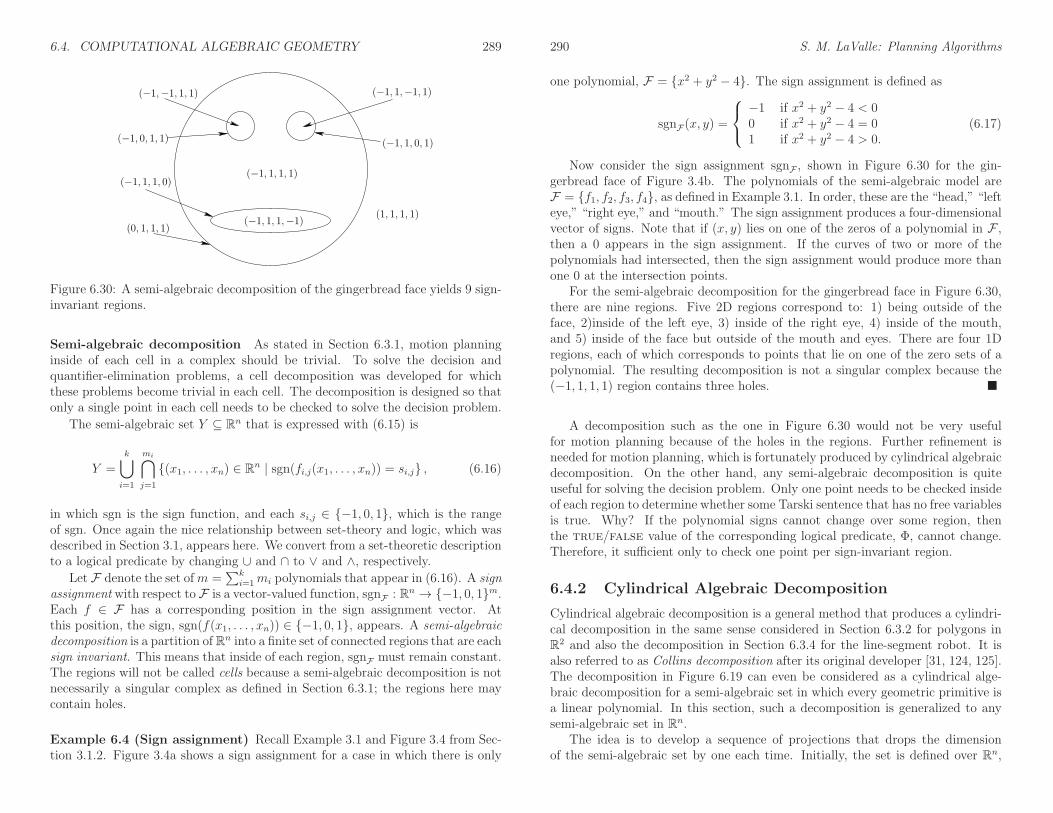
6.4. COMPUTATIONAL ALGEBRAIC GEOMETRY 289
(−1,−1, 1, 1) (−1, 1,−1, 1)
(−1, 1, 1, 0)
(−1, 1, 0, 1)(−1, 0, 1, 1)
(1, 1, 1, 1)
(0, 1, 1, 1)(−1, 1, 1,−1)
(−1, 1, 1, 1)
Figure 6.30: A semi-algebraic decomposition of the gingerbread face yields 9 sign-invariant regions.
Semi-algebraic decomposition As stated in Section 6.3.1, motion planninginside of each cell in a complex should be trivial. To solve the decision andquantifier-elimination problems, a cell decomposition was developed for whichthese problems become trivial in each cell. The decomposition is designed so thatonly a single point in each cell needs to be checked to solve the decision problem.
The semi-algebraic set Y ⊆ Rn that is expressed with (6.15) is
Y =k⋃
i=1
mi⋂
j=1
(x1, . . . , xn) ∈ Rn | sgn(fi,j(x1, . . . , xn)) = si,j , (6.16)
in which sgn is the sign function, and each si,j ∈ −1, 0, 1, which is the rangeof sgn. Once again the nice relationship between set-theory and logic, which wasdescribed in Section 3.1, appears here. We convert from a set-theoretic descriptionto a logical predicate by changing ∪ and ∩ to ∨ and ∧, respectively.
Let F denote the set ofm =∑k
i=1mi polynomials that appear in (6.16). A signassignment with respect to F is a vector-valued function, sgnF : Rn → −1, 0, 1m.Each f ∈ F has a corresponding position in the sign assignment vector. Atthis position, the sign, sgn(f(x1, . . . , xn)) ∈ −1, 0, 1, appears. A semi-algebraicdecomposition is a partition of Rn into a finite set of connected regions that are eachsign invariant. This means that inside of each region, sgnF must remain constant.The regions will not be called cells because a semi-algebraic decomposition is notnecessarily a singular complex as defined in Section 6.3.1; the regions here maycontain holes.
Example 6.4 (Sign assignment) Recall Example 3.1 and Figure 3.4 from Sec-tion 3.1.2. Figure 3.4a shows a sign assignment for a case in which there is only
290 S. M. LaValle: Planning Algorithms
one polynomial, F = x2 + y2 − 4. The sign assignment is defined as
sgnF(x, y) =
−1 if x2 + y2 − 4 < 00 if x2 + y2 − 4 = 01 if x2 + y2 − 4 > 0.
(6.17)
Now consider the sign assignment sgnF , shown in Figure 6.30 for the gin-gerbread face of Figure 3.4b. The polynomials of the semi-algebraic model areF = f1, f2, f3, f4, as defined in Example 3.1. In order, these are the “head,” “lefteye,” “right eye,” and “mouth.” The sign assignment produces a four-dimensionalvector of signs. Note that if (x, y) lies on one of the zeros of a polynomial in F ,then a 0 appears in the sign assignment. If the curves of two or more of thepolynomials had intersected, then the sign assignment would produce more thanone 0 at the intersection points.
For the semi-algebraic decomposition for the gingerbread face in Figure 6.30,there are nine regions. Five 2D regions correspond to: 1) being outside of theface, 2)inside of the left eye, 3) inside of the right eye, 4) inside of the mouth,and 5) inside of the face but outside of the mouth and eyes. There are four 1Dregions, each of which corresponds to points that lie on one of the zero sets of apolynomial. The resulting decomposition is not a singular complex because the(−1, 1, 1, 1) region contains three holes.
A decomposition such as the one in Figure 6.30 would not be very usefulfor motion planning because of the holes in the regions. Further refinement isneeded for motion planning, which is fortunately produced by cylindrical algebraicdecomposition. On the other hand, any semi-algebraic decomposition is quiteuseful for solving the decision problem. Only one point needs to be checked insideof each region to determine whether some Tarski sentence that has no free variablesis true. Why? If the polynomial signs cannot change over some region, thenthe true/false value of the corresponding logical predicate, Φ, cannot change.Therefore, it sufficient only to check one point per sign-invariant region.
6.4.2 Cylindrical Algebraic Decomposition
Cylindrical algebraic decomposition is a general method that produces a cylindri-cal decomposition in the same sense considered in Section 6.3.2 for polygons inR2 and also the decomposition in Section 6.3.4 for the line-segment robot. It isalso referred to as Collins decomposition after its original developer [31, 124, 125].The decomposition in Figure 6.19 can even be considered as a cylindrical alge-braic decomposition for a semi-algebraic set in which every geometric primitive isa linear polynomial. In this section, such a decomposition is generalized to anysemi-algebraic set in Rn.
The idea is to develop a sequence of projections that drops the dimensionof the semi-algebraic set by one each time. Initially, the set is defined over Rn,

6.4. COMPUTATIONAL ALGEBRAIC GEOMETRY 291
and after one projection, a semi-algebraic set is obtained in Rn−1. Eventually,the projection reaches R, and a univariate polynomial is obtained for which thezeros are at the critical places where cell boundaries need to be formed. A celldecomposition of 1-cells (intervals) and 0-cells is formed by partitioning R. Thesequence is then reversed, and decompositions are formed from R2 up to Rn. Eachiteration starts with a cell decomposition in Ri and lifts it to obtain a cylinder ofcells in Ri+1. Figure 6.35 shows how the decomposition looks for the gingerbreadexample; since n = 2, it only involves one projection and one lifting.
Semi-algebraic projections are semi-algebraic The following is implied bythe Tarski-Seidenberg Theorem [53]:
A projection of a semi-algebraic set from dimension n to dimensionn− 1 is a semi-algebraic set.
This gives a kind of closure of semi-algebraic sets under projection, which is re-quired to ensure that every projection of a semi-algebraic set in Ri leads to asemi-algebraic set in Ri−1. This property is actually not true for (real) algebraicvarieties, which were introduced in Section 4.4.1. Varieties are defined using onlythe = relation and are not closed under the projection operation. Therefore, it isa good thing (not just a coincidence!) that we are using semi-algebraic sets.
Real algebraic numbers As stated previously, the sequence of projections endswith a univariate polynomial over R. The sides of the cells will be defined basedon the precise location of the roots of this polynomial. Furthermore, representinga sample point for a cell of dimension k in a complex in Rn for k < n requiresperfect precision. If the coordinates are slightly off, the point will lie in a differentcell. This raises the complicated issue of how these roots are represented andmanipulated in a computer.
For univariate polynomials of degree 4 or less, formulas exist to compute allof the roots in terms of functions of square roots and higher order roots. FromGalois theory [244, 394], it is known that such formulas and nice expressions forroots do not exist for most higher degree polynomials, which can certainly arisein the complicated semi-algebraic models that are derived in motion planning.The roots in R could be any real number, and many real numbers require infiniterepresentations.
One way of avoiding this mess is to assume that only polynomials inQ[x1, . . . , xn]are used, instead of the more general R[x1, . . . , xn]. The field Q is not alge-braically closed because zeros of the polynomials lie outside of Qn. For example, iff(x1) = x21 − 2, then f = 0 for x1 = ±
√2, and
√2 6∈ Q. However, some elements
of R can never be roots of a polynomial in Q[x1, . . . , xn].The set A of all real roots to all polynomials in Q[x] is called the set of real
algebraic numbers. The set A ⊂ R actually represents a field (recall from Section4.4.1). Several nice algorithmic properties of the numbers in A are 1) they all have
292 S. M. LaValle: Planning Algorithms
finite representations, 2) addition and multiplication operations on elements of Acan be computed in polynomial time, and 3) conversions between different repre-sentations of real algebraic numbers can be performed in polynomial time. Thismeans that all operations can be computed efficiently without resorting to somekind of numerical approximation. In some applications, such approximations arefine; however, for algebraic decompositions, they destroy critical information bypotentially confusing roots (e.g., how can we know for sure whether a polynomialhas a double root or just two roots that are very close together?).
The details are not presented here, but there are several methods for rep-resenting real algebraic numbers and the corresponding algorithms for manipu-lating them efficiently. The running time of cylindrical algebraic decompositionultimately depends on this representation. In practice, a numerical root-findingmethod that has a precision parameter, ǫ, can be used by choosing ǫ small enoughto ensure that roots will not be confused. A sufficiently small value can be de-termined by applying gap theorems, which give lower bounds on the amount ofreal root separation, expressed in terms of the polynomial coefficients [92]. Somemethods avoid requiring a precision parameter. One well-known example is thederivation of a Sturm sequence of polynomials based on the given polynomial.The polynomials in the Sturm sequence are then used to find isolating intervalsfor each of the roots [53]. The polynomial, together with its isolating interval, canbe considered as an exact root representation. Algebraic operations can even beperformed using this representation in time O(d lg2 d), in which d is the degreeof the polynomial [428]. See [53, 92, 428] for detailed presentations on the exactrepresentation and calculation with real algebraic numbers.
One-dimensional decomposition To explain the cylindrical algebraic decom-position method, we first perform a semi-algebraic decomposition of R, which isthe final step in the projection sequence. Once this is explained, then the multi-dimensional case follows more easily.
Let F be a set of m univariate polynomials,
F = fi ∈ Q[x] | i = 1, . . . ,m, (6.18)
which are used to define some semi-algebraic set in R. The polynomials in F couldcome directly from a quantifier-free formula φ (which could even appear inside ofa Tarski sentence, as in (6.9)).
Define a single polynomial as f =∏m
i=1 fi. Suppose that f has k distinct, realroots, which are sorted in increasing order:
−∞ < β1 < β2 < · · · < βi−1 < βi < βi+1 < · · · < βk < ∞. (6.19)
The one-dimensional semi-algebraic decomposition is given by the followingsequence of alternating 1-cells and 0-cells:
(−∞, β1), [β1, β1], (β1, β2), . . . , (βi−1, βi), [βi, βi],
(βi, βi+1), . . . , [βk, βk], (βk,∞).(6.20)
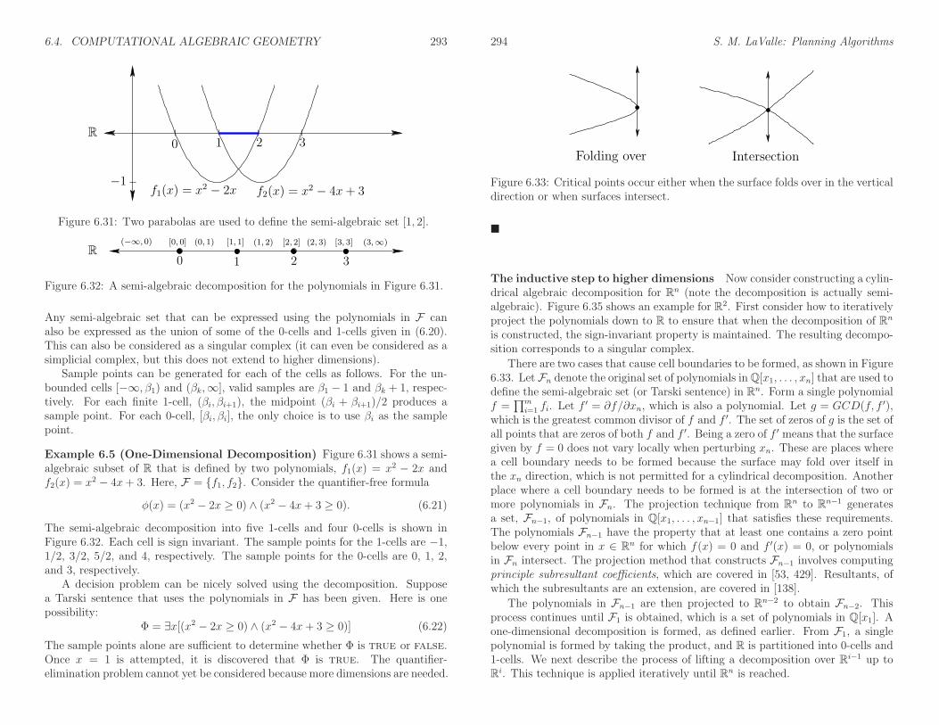
6.4. COMPUTATIONAL ALGEBRAIC GEOMETRY 293
f1(x) = x2 − 2x f2(x) = x2 − 4x + 3
2 310R
−1
Figure 6.31: Two parabolas are used to define the semi-algebraic set [1, 2].
R0
[3, 3](2, 3)(1, 2)[1, 1] [2, 2](0, 1)[0, 0](−∞, 0) (3,∞)
2 31
Figure 6.32: A semi-algebraic decomposition for the polynomials in Figure 6.31.
Any semi-algebraic set that can be expressed using the polynomials in F canalso be expressed as the union of some of the 0-cells and 1-cells given in (6.20).This can also be considered as a singular complex (it can even be considered as asimplicial complex, but this does not extend to higher dimensions).
Sample points can be generated for each of the cells as follows. For the un-bounded cells [−∞, β1) and (βk,∞], valid samples are β1 − 1 and βk + 1, respec-tively. For each finite 1-cell, (βi, βi+1), the midpoint (βi + βi+1)/2 produces asample point. For each 0-cell, [βi, βi], the only choice is to use βi as the samplepoint.
Example 6.5 (One-Dimensional Decomposition) Figure 6.31 shows a semi-algebraic subset of R that is defined by two polynomials, f1(x) = x2 − 2x andf2(x) = x2 − 4x+ 3. Here, F = f1, f2. Consider the quantifier-free formula
φ(x) = (x2 − 2x ≥ 0) ∧ (x2 − 4x+ 3 ≥ 0). (6.21)
The semi-algebraic decomposition into five 1-cells and four 0-cells is shown inFigure 6.32. Each cell is sign invariant. The sample points for the 1-cells are −1,1/2, 3/2, 5/2, and 4, respectively. The sample points for the 0-cells are 0, 1, 2,and 3, respectively.
A decision problem can be nicely solved using the decomposition. Supposea Tarski sentence that uses the polynomials in F has been given. Here is onepossibility:
Φ = ∃x[(x2 − 2x ≥ 0) ∧ (x2 − 4x+ 3 ≥ 0)] (6.22)
The sample points alone are sufficient to determine whether Φ is true or false.Once x = 1 is attempted, it is discovered that Φ is true. The quantifier-elimination problem cannot yet be considered because more dimensions are needed.
294 S. M. LaValle: Planning Algorithms
Folding over Intersection
Figure 6.33: Critical points occur either when the surface folds over in the verticaldirection or when surfaces intersect.
The inductive step to higher dimensions Now consider constructing a cylin-drical algebraic decomposition for Rn (note the decomposition is actually semi-algebraic). Figure 6.35 shows an example for R2. First consider how to iterativelyproject the polynomials down to R to ensure that when the decomposition of Rn
is constructed, the sign-invariant property is maintained. The resulting decompo-sition corresponds to a singular complex.
There are two cases that cause cell boundaries to be formed, as shown in Figure6.33. Let Fn denote the original set of polynomials inQ[x1, . . . , xn] that are used todefine the semi-algebraic set (or Tarski sentence) in Rn. Form a single polynomialf =
∏mi=1 fi. Let f ′ = ∂f/∂xn, which is also a polynomial. Let g = GCD(f, f ′),
which is the greatest common divisor of f and f ′. The set of zeros of g is the set ofall points that are zeros of both f and f ′. Being a zero of f ′ means that the surfacegiven by f = 0 does not vary locally when perturbing xn. These are places wherea cell boundary needs to be formed because the surface may fold over itself inthe xn direction, which is not permitted for a cylindrical decomposition. Anotherplace where a cell boundary needs to be formed is at the intersection of two ormore polynomials in Fn. The projection technique from Rn to Rn−1 generatesa set, Fn−1, of polynomials in Q[x1, . . . , xn−1] that satisfies these requirements.The polynomials Fn−1 have the property that at least one contains a zero pointbelow every point in x ∈ Rn for which f(x) = 0 and f ′(x) = 0, or polynomialsin Fn intersect. The projection method that constructs Fn−1 involves computingprinciple subresultant coefficients, which are covered in [53, 429]. Resultants, ofwhich the subresultants are an extension, are covered in [138].
The polynomials in Fn−1 are then projected to Rn−2 to obtain Fn−2. Thisprocess continues until F1 is obtained, which is a set of polynomials in Q[x1]. Aone-dimensional decomposition is formed, as defined earlier. From F1, a singlepolynomial is formed by taking the product, and R is partitioned into 0-cells and1-cells. We next describe the process of lifting a decomposition over Ri−1 up toRi. This technique is applied iteratively until Rn is reached.

6.4. COMPUTATIONAL ALGEBRAIC GEOMETRY 295
Assume inductively that a cylindrical algebraic decomposition has been com-puted for a set of polynomials Fi−1 in Q[x1, . . . , xi−1]. The decomposition consistsof k-cells for which 0 ≤ k ≤ i. Let p = (x1, . . . , xi−1) ∈ Ri−1. For each one of thek-cells Ci−1, a cylinder over Ci−1 is defined as the (k + 1)-dimensional set
(p, xi) ∈ Ri | p ∈ Ci−1. (6.23)
The cylinder is sliced into a strip of k-dimensional and k+ 1-dimensional cells byusing polynomials in Fi. Let fj denote one of the ℓ slicing polynomials in thecylinder, sorted in increasing xi order as f1, f2, . . ., fj, fj+1, . . ., fℓ. The followingkinds of cells are produced (see Figure 6.34):
1. Lower unbounded sector:
(p, xi) ∈ Ri | p ∈ Ci−1 and xi < f1(p) . (6.24)
2. Section:(p, xi) ∈ Ri | p ∈ Ci−1 and xi = fj(p) . (6.25)
3. Bounded sector:
(p, xi) ∈ Ri | p ∈ Ci−1 and fj(p) < xi < fj+1(p) . (6.26)
4. Upper unbounded sector:
(p, xi) ∈ Ri | p ∈ Ci−1 and fℓ(p) < xi . (6.27)
There is one degenerate possibility in which there are no slicing polynomials andthe cylinder over Ci−1 can be extended into one unbounded cell. In general, thesample points are computed by picking a point in p ∈ Ci−1 and making a verticalcolumn of samples of the form (p, xi). A polynomial in Q[xi] can be generated,and the samples are placed using the same assignment technique that was usedfor the one-dimensional decomposition.
Example 6.6 (Mutilating the Gingerbread Face) Figure 6.35 shows a cylin-drical algebraic decomposition of the gingerbread face. Observe that the resultingcomplex is very similar to that obtained in Figure 6.19.
Note that the cells do not necessarily project onto a rectangular set, as in thecase of a higher dimensional vertical decomposition. For example, a generic n-cellCn for a decomposition of Rn is described as the open set of (x1, . . . , xn) ∈ Rn
such that
• C0 < xn < C ′0 for some 0-cells C0, C
′0 ∈ R, which are roots of some f, f ′ ∈ F1.
296 S. M. LaValle: Planning Algorithms
f1
fj
Ci−1
fj+1
fℓ
Figure 6.34: A cylinder over every k-cell Ci−1 is formed. A sequence of poly-nomials, f1, . . ., fℓ, slices the cylinder into k-dimensional sections and (k + 1)-dimensional sectors.
• (xn−1, xn) lies between C1 and C ′1 for some 1-cells C1, C
′1, which are zeros
of some f, f ′ ∈ F2.
...
• (xn−i+1, . . . , xn) lies between Ci−1 and C′i−1 for some i-cells Ci−1, C
′i−1, which
are zeros of some f, f ′ ∈ Fi.
...
• (x1, . . . , xn) lies between Cn−1 and C ′n−1 for some (n − 1)-cells Cn−1, C
′n−1,
which are zeros of some f, f ′ ∈ Fn.
The resulting decomposition is sign invariant, which allows the decision andquantifier-elimination problems to be solved in finite time. To solve a decisionproblem, the polynomials in Fn are evaluated at every sample point to deter-mine whether one of them satisfies the Tarski sentence. To solve the quantifier-elimination problem, note that any semi-algebraic sets that can be constructedfrom Fn can be defined as a union of some cells in the decomposition. For thegiven Tarski sentence, Fn is formed from all polynomials that are mentioned in
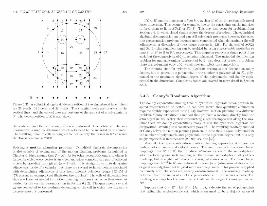
6.4. COMPUTATIONAL ALGEBRAIC GEOMETRY 297
3
5
6
7
9
10
11
12
1 13
14
15
16
17
18
19
20
21
22
23
24
25
26
27
28
29
328
33
342
35
30
364
37
31
R
Figure 6.35: A cylindrical algebraic decomposition of the gingerbread face. Thereare 37 2-cells, 64 1-cells, and 28 0-cells. The straight 1-cells are intervals of thevertical lines, and the curved ones are portions of the zero set of a polynomial inF . The decomposition of R is also shown.
the sentence, and the cell decomposition is performed. Once obtained, the signinformation is used to determine which cells need to be included in the union.The resulting union of cells is designed to include only the points in Rn at whichthe Tarski sentence is true.
Solving a motion planning problem Cylindrical algebraic decompositionis also capable of solving any of the motion planning problems formulated inChapter 4. First assume that C = Rn. As for other decompositions, a roadmap isformed in which every vertex is an n-cell and edges connect every pair of adjacentn-cells by traveling through an (n − 1)-cell. It is straightforward to determineadjacencies inside of a cylinder, but there are several technical details associatedwith determining adjacencies of cells from different cylinders (pages 152–154 of[53] present an example that illustrates the problem). The cells of dimension lessthan n− 1 are not needed for motion planning purposes (just as vertices were notneeded for the vertical decomposition in Section 6.2.2). The query points qI andqG are connected to the roadmap depending on the cell in which they lie, and adiscrete search is performed.
298 S. M. LaValle: Planning Algorithms
If C ⊂ Rn and its dimension is k for k < n, then all of the interesting cells are oflower dimension. This occurs, for example, due to the constraints on the matricesto force them to lie in SO(2) or SO(3). This may also occur for problems fromSection 4.4, in which closed chains reduce the degrees of freedom. The cylindricalalgebraic decomposition method can still solve such problems; however, the exactroot representation problem becomes more complicated when determining the celladjacencies. A discussion of these issues appears in [428]. For the case of SO(2)and SO(3), this complication can be avoided by using stereographic projection tomap S1 or S3 to R or R3, respectively. This mapping removes a single point fromeach, but the connectivity of Cfree remains unharmed. The antipodal identificationproblem for unit quaternions represented by S3 also does not present a problem;there is a redundant copy of C, which does not affect the connectivity.
The running time for cylindrical algebraic decomposition depends on manyfactors, but in general it is polynomial in the number of polynomials in Fn, poly-nomial in the maximum algebraic degree of the polynomials, and doubly expo-nential in the dimension. Complexity issues are covered in more detail in Section6.5.3.
6.4.3 Canny’s Roadmap Algorithm
The doubly exponential running time of cylindrical algebraic decomposition in-spired researchers to do better. It has been shown that quantifier eliminationrequires doubly exponential time [144]; however, motion planning is a differentproblem. Canny introduced a method that produces a roadmap directly from thesemi-algebraic set, rather than constructing a cell decomposition along the way.Since there are doubly exponentially many cells in the cylindrical algebraic de-composition, avoiding this construction pays off. The resulting roadmap methodof Canny solves the motion planning problem in time that is again polynomial inthe number of polynomials and polynomial in the algebraic degree, but it is onlysingly exponential in dimension [90, 92]; see also [53].
Much like the other combinatorial motion planning approaches, it is based onfinding critical curves and critical points. The main idea is to construct linearmappings from Rn to R2 that produce silhouette curves of the semi-algebraicsets. Performing one such mapping on the original semi-algebraic set yields aroadmap, but it might not preserve the original connectivity. Therefore, linearmappings from Rn−1 to R2 are performed on some (n−1)-dimensional slices of theoriginal semi-algebraic set to yield more roadmap curves. This process is appliedrecursively until the slices are already one-dimensional. The resulting roadmapis formed from the union of all of the pieces obtained in the recursive calls. Theresulting roadmap has the same connectivity as the original semi-algebraic set[92].
Suppose that C = Rn. Let F = f1, . . . , fm denote the set of polynomialsthat define the semi-algebraic set, which is assumed to be a disjoint union of

6.4. COMPUTATIONAL ALGEBRAIC GEOMETRY 299
manifolds. Assume that each fi ∈ Q[x1, . . . , xn]. First, a small perturbation tothe input polynomials F is performed to ensure that every sign-invariant set of Rn
is a manifold. This forces the polynomials into a kind of general position, whichcan be achieved with probability one using random perturbations; there are alsodeterministic methods to solve this problem. The general position requirementson the input polynomials and the 2D projection directions are fairly strong, whichhas stimulated more recent work that eliminates many of the problems [53]. Fromthis point onward, it will be assumed that the polynomials are in general position.
Recall the sign-assignment function from Section 6.4.1. Each sign-invariantset is a manifold because of the general position assumption. Canny’s methodcomputes a roadmap for any k-dimensional manifold for k < n. Such a manifoldhas precisely n − k signs that are 0 (which means that points lie precisely onthe zero sets of n − k polynomials in F). At least one of the signs must be 0,which means that Canny’s roadmap actually lies in ∂Cfree (this technically is notpermitted, but the algorithm nevertheless correctly decides whether a solutionpath exists through Cfree).
Recall that each fi is a function, fi : Rn → R. Let x denote (x1, . . . , xn) ∈ Rn.
The k polynomials that have zero signs can be put together sequentially to producea mapping ψ : Rn → Rk. The ith component of the vector ψ(x) is ψi(x) = fi(x).This is closely related to the sign assignment function of Section 6.4.1, except thatnow the real value from each polynomial is directly used, rather than taking itssign.
Now introduce a function g : Rn → Rj, in which either j = 1 or j = 2 (thegeneral concepts presented below work for other values of j, but 1 and 2 are theonly values needed for Canny’s method). The function g serves the same purposeas a projection in cylindrical algebraic decomposition, but note that g immediatelydrops from dimension n to dimension 2 or 1, instead of dropping to n − 1 as inthe case of cylindrical projections.
Let h : Rn → Rk+j denote a mapping constructed directly from ψ and g asfollows. For the ith component, if i ≤ k, then hi(x) = ψi(x) = fi(x). Assumethat k + j ≤ n. If i > k, then hi(x) = gi−k(x). Let Jx(h) denote the Jacobian ofh and be defined at x as
Jx(h) =
∂h1(x)
∂x1· · · ∂h1(x)
∂xn...
...∂hm+k(x)
∂x1· · · ∂hm+k(x)
∂xn
=
∂f1(x)
∂x1· · · ∂f1(x)
∂xn...
...∂fk(x)
∂x1· · · ∂fk(x)
∂xn
∂g1(x)
∂x1· · · ∂g1(x)
∂xn...
...∂gj(x)
∂x1· · · ∂gj(x)
∂xn
. (6.28)
300 S. M. LaValle: Planning Algorithms
A point x ∈ Rn at which Jx(h) is singular is called a critical point. The matrix isdefined to be singular if every (m+k)×(m+k) subdeterminant is zero. Each of thefirst k rows of Jx(h) calculates the surface normal to fi(x) = 0. If these normalsare not linearly independent of the directions given by the last j rows, then thematrix becomes singular. The following example from [89] nicely illustrates thisprinciple.
Example 6.7 (Canny’s Roadmap Algorithm) Let n = 3, k = 1, and j = 1.The zeros of a single polynomial f1 define a 2D subset of R3. Let f1 be the unitsphere, S2, defined as the zeros of the polynomial
f1(x1, x2, x3) = x21 + x22 + x23 − 1. (6.29)
Suppose that g : R3 → R is defined as g(x1, x2, x3) = x1. The Jacobian, (6.28),becomes
(
2x1 2x2 2x31 0 0
)
(6.30)
and is singular when all three of the possible 2 × 2 subdeterminants are zero.This occurs if and only if x2 = x3 = 0. This yields the critical points (−1, 0, 0)and (1, 0, 0) on S2. Note that this is precisely when the surface normals of S2 areparallel to the vector [1 0 0].
Now suppose that j = 2 to obtain g : R3 → R2, and suppose g(x1, x2, x3) =(x1, x2). In this case, (6.28) becomes
2x1 2x2 2x31 0 00 1 0
, (6.31)
which is singular if and only if x3 = 0. The critical points are therefore the x1x2plane intersected with S3, which yields the equator points (all (x1, x2) ∈ R2 suchthat x21 + x22 = 1). In this case, more points are generated because the matrixbecomes degenerate for any surface normal of S2 that is parallel to [1 0 0], [0 1 0]or any linear combination of these.
The first mapping in Example 6.7 yielded two isolated critical points, and thesecond mapping yielded a one-dimensional set of critical points, which is referredto as a silhouette. The union of the silhouette and the isolated critical pointsyields a roadmap for S2. Now consider generalizing this example to obtain thefull algorithm for general n and k. A linear mapping g : Rn → R2 is constructedthat might not be axis-aligned as in Example 6.7 because it must be chosen ingeneral position (otherwise degeneracies might arise in the roadmap). Define ψ tobe the set of polynomials that become zero on the desired manifold on which toconstruct a roadmap. Form the matrix (6.28) and determine the silhouette. Thisis accomplished in general using subresultant techniques that were also needed

6.4. COMPUTATIONAL ALGEBRAIC GEOMETRY 301
for cylindrical algebraic decomposition; see [53, 92] for details. Let g1 denote thefirst component of g, which yields a mapping g1 : R
n → R. Forming (6.28) usingg1 yields a finite set of critical points. Taking the union of the critical points andthe silhouette produces part of the roadmap.
So far, however, there are no guarantees that the connectivity is preserved.To handle this problem, Canny’s algorithm proceeds recursively. For each of thecritical points x ∈ Rn, an n − 1-dimensional hyperplane through x is chosen forwhich the g1 row of (6.28) is the normal (hence it is perpendicular in some sense tothe flow of g1). Inside of this hyperplane, a new g mapping is formed. This timea new direction is chosen, and the mapping takes the form g : Rn−1 → R2. Onceagain, the silhouettes and critical points are found and added to the roadmap.This process is repeated recursively until the base case in which the silhouettesand critical points are directly obtained without forming g.
It is helpful to consider an example. Since the method involves a sequence of2D projections, it is difficult to visualize. Problems in R4 and higher involve twoor more 2D projections and would therefore be more interesting. An example overR3 is presented here, even though it unfortunately has only one projection; see[92] for another example over R3.
Example 6.8 (Canny’s Algorithm on a Torus) Consider the 3D algebraic setshown in Figure 6.36. After defining the mapping g(x1, x2, x3) = (x1, x2), theroadmap shown in Figure 6.37 is obtained. The silhouettes are obtained from g,and the critical points are obtained from g1 (this is the first component of g).Note that the original connectivity of the solid torus is not preserved because theinner ring does not connect to the outer ring. This illustrates the need to alsocompute the roadmap for lower dimensional slices. For each of the four criticalpoints, the critical curves are computed for a plane that is parallel to the x2x3plane and for which the x1 position is determined by the critical point. The slicefor one of the inner critical points is shown in Figure 6.38. In this case, the slicealready has two dimensions. New silhouette curves are added to the roadmap toobtain the final result shown in Figure 6.39.
To solve a planning problem, the query points qI and qG are artificially declaredto be critical points in the top level of recursion. This forces the algorithm togenerate curves that connect them to the rest of the roadmap.
The completeness of the method requires very careful analysis, which is thor-oughly covered in [53, 92]. The main elements of the analysis are showing that:1) the polynomials can be perturbed and g can be chosen to ensure general po-sition, 2) the singularity conditions on (6.28) lead to algebraic sets (varieties),and 3) the resulting roadmap has the required properties mentioned in Section6.1 of being accessible and connectivity-preserving for Cfree (actually it is shownfor ∂Cfree). The method explained above computes the roadmap for each sign-invariant set, but to obtain a roadmap for the planning problem, the roadmaps
302 S. M. LaValle: Planning Algorithms
x1
x3
x2
Figure 6.36: Suppose that the semi-algebraic set is a solid torus in R3.
Figure 6.37: The projection into the x1x2 plane yields silhouettes for the innerand outer rings and also four critical points.
Figure 6.38: A slice taken for the inner critical points is parallel to the x2x3 plane.The roadmap for the slice connects to the silhouettes from Figure 6.37, therebypreserving the connectivity of the original set in Figure 6.36.
Figure 6.39: All of the silhouettes and critical points are merged to obtain theroadmap.

6.5. COMPLEXITY OF MOTION PLANNING 303
from each sign-invariant set must be connected together correctly; fortunately, thishas been solved via the Linking Lemma of [89]. A major problem, however, is thateven after knowing the connectivity of the roadmap, it is a considerable challengeto obtain a parameterization of each curve on the roadmap. For this and manyother technical reasons, no general implementation of Canny’s algorithm appearsto exist at present. Another problem is the requirement of a Whitney stratifica-tion (which can be fixed by perturbation of the input). The Basu-Pollack-Royroadmap algorithm overcomes this problem [53].
6.5 Complexity of Motion Planning
This section summarizes theoretical work that characterizes the complexity ofmotion planning problems. Note that this is not equivalent to characterizing therunning time of particular algorithms. The existence of an algorithm serves asan upper bound on the problem’s difficulty because it is a proof by example thatsolving the problem requires no more time than what is needed by the algorithm.On the other hand, lower bounds are also very useful because they give an indica-tion of the difficulty of the problem itself. Suppose, for example, you are given analgorithm that solves a problem in time O(n2). Does it make sense to try to finda more efficient algorithm? Does it make sense to try to find a general-purposemotion planning algorithm that runs in time that is polynomial in the dimension?Lower bounds provide answers to questions such as this. Usually lower boundsare obtained by concocting bizarre, complicated examples that are allowed by theproblem definition but were usually not considered by the person who first for-mulated the problem. In this line of research, progress is made by either raisingthe lower bound (unless it is already tight) or by showing that a narrower versionof the problem still allows such bizarre examples. The latter case occurs often inmotion planning.
6.5.1 Lower Bounds
Lower bounds have been established for a variety of motion planning problemsand also a wide variety of planning problems in general. To interpret these boundsa basic understanding of the theory of computation is required [239, 442]. Thisfascinating subject will be unjustly summarized in a few paragraphs. A problemis a set of instances that are each carefully encoded as a binary string. An algo-rithm is formally considered as a Turing machine, which is a finite-state machinethat can read and write bits to an unbounded piece of tape. Other models ofcomputation also exist, such as integer RAM and real RAM (see [65]); there aredebates as to which model is most appropriate, especially when performing ge-ometric computations with real numbers. The standard Turing machine modelwill be assumed from here onward. Algorithms are usually formulated to makea binary output, which involves accepting or rejecting a problem instance that is
304 S. M. LaValle: Planning Algorithms
P NP PSPACE EXPTIME
Figure 6.40: It is known that P ⊂ EXPTIME is a strict subset; however, it is notknown precisely how large NP and PSPACE are.
initially written to the tape and given to the algorithm. In motion planning, thisamounts to deciding whether a solution path exists for a given problem instance.
Languages A language is a set of binary strings associated with a problem. Itrepresents the complete set of instances of a problem. An algorithm is said todecide a language if in finite time it correctly accepts all strings that belong toit and rejects all others. The interesting question is: How much time or space isrequired to decide a language? This question is asked of the problem, under theassumption that the best possible algorithm would be used to decide it. (We caneasily think of inefficient algorithms that waste resources.)
A complexity class is a set of languages that can all be decided within somespecified resource bound. The class P is the set of all languages (and henceproblems) for which a polynomial-time algorithm exists (i.e., the algorithm runsin time O(nk) for some integer k). By definition, an algorithm is called efficientif it decides its associated language in polynomial time.7 If no efficient algorithmexists, then the problem is called intractable. The relationship between severalother classes that often emerge in theoretical motion planning is shown in Figure6.40. The class NP is the set of languages that can be solved in polynomialtime by a nondeterministic Turing machine. Some discussion of nondeterministicmachines appears in Section 11.3.2. Intuitively, it means that solutions can beverified in polynomial time because the machine magically knows which choicesto make while trying to make the decision. The class PSPACE is the set oflanguages that can be decided with no more than a polynomial amount of storagespace during the execution of the algorithm (NPSPACE=PSPACE, so there isno nondeterministic version). The class EXPTIME is the set of languages thatcan be decided in time O(2n
k
) for some integer k. It is known that EXPTIMEis larger than P, but it is not known precisely where the boundaries of NP andPSPACE lie. It might be the case that P = NP = PSPACE (although hardlyanyone believes this), or it could be that NP = PSPACE = EXPTIME.
7Note that this definition may be absurd in practice; an algorithm that runs in time O(n90125)would probably not be too efficient for most purposes.

6.5. COMPLEXITY OF MOTION PLANNING 305
Figure 6.41: Even motion planning for a bunch of translating rectangles inside ofa rectangular box in R2 is PSPACE-hard (and hence, NP-hard).
Hardness and completeness Since an easier class is included as a subset ofa harder one, it is helpful to have a notion of a language (i.e., problem) beingamong the hardest possible within a class. Let X refer to either P, NP, PSPACE,or EXPTIME. A language A is called X-hard if every language B in class X ispolynomial-time reducible to A. In short, this means that in polynomial time,any language in B can be translated into instances for language A, and then thedecisions for A can be correctly translated back in polynomial time to correctlydecide B. Thus, if A can be decided, then within a polynomial-time factor, everylanguage in X can be decided. The hardness concept can even be applied toa language (problem) that does not belong to the class. For example, we candeclare that a language A is NP-hard even if A 6∈NP (it could be harder and lie inEXPTIME, for example). If it is known that the language is both hard for someclass X and is also a member of X, then it is called X-complete (i.e., NP-complete,PSPACE-complete, etc.).8 Note that because of this uncertainty regarding P, NP,and PSPACE, one cannot say that a problem is intractable if it is NP-hard orPSPACE-hard, but one can, however, if the problem is EXPTIME-hard. Oneadditional remark: it is useful to remember that PSPACE-hard implies NP-hard.
Lower bounds for motion planning The general motion planning problem,Formulation 4.1, was shown in 1979 to be PSPACE-hard by Reif [409]. In fact, the
8If you remember hearing that a planning problem is NP-something, but cannot rememberwhether it was NP-hard or NP-complete, then it is safe to say NP-hard because NP-completeimplies NP-hard. This can similarly be said for other classes, such as PSPACE-complete vs.PSPACE-hard.
306 S. M. LaValle: Planning Algorithms
problem was restricted to polyhedral obstacles and a finite number of polyhedralrobot bodies attached by spherical joints. The coordinates of all polyhedra areassumed to be in Q (this enables a finite-length string encoding of the probleminstance). The proof introduces a fascinating motion planning instance that in-volves many attached, dangling robot parts that must work their way through acomplicated system of tunnels, which together simulates the operation of a sym-metric Turing machine. Canny later established that the problem in Formulation4.1 (expressed using polynomials that have rational coefficients) lies in PSPACE[92]. Therefore, the general motion planning problem is PSPACE-complete.
Many other lower bounds have been shown for a variety of planning problems.One famous example is the Warehouseman’s problem shown in Figure 6.41. Thisproblem involves a finite number of translating, axis-aligned rectangles in a rect-angular world. It was shown in [238] to be PSPACE-hard. This example is abeautiful illustration of how such a deceptively simple problem formulation canlead to such a high lower bound. More recently, it was even shown that planningfor Sokoban, which is a warehouseman’s problem on a discrete 2D grid, is alsoPSPACE-hard [141]. Other general motion planning problems that were shownto be PSPACE-hard include motion planning for a chain of bodies in the plane[237, 254] and motion planning for a chain of bodies among polyhedral obsta-cles in R3. Many lower bounds have been established for a variety of extensionsand variations of the general motion planning problem. For example, in [91] itwas established that a certain form of planning under uncertainty for a robot ina 3D polyhedral environment is NEXPTIME-hard, which is harder than any ofthe classes shown in Figure 6.40; the hardest problems in this NEXPTIME arebelieved to require doubly exponential time to solve.
The lower bound or hardness results depend significantly on the precise repre-sentation of the problem. For example, it is possible to make problems look easierby making instance encodings that are exponentially longer than they should be.The running time or space required is expressed in terms of n, the input size. Ifthe motion planning problem instances are encoded with exponentially more bitsthan necessary, then a language that belongs to P is obtained. As long as theinstance encoding is within a polynomial factor of the optimal encoding (this canbe made precise using Kolmogorov complexity [323]), then this bizarre behavioris avoided. Another important part of the representation is to pay attention tohow parameters in the problem formulation can vary. We can redefine motionplanning to be all instances for which the dimension of C is never greater than21000. The number of dimensions is sufficiently large for virtually any application.The resulting language for this problem belongs to P because cylindrical algebraicdecomposition and Canny’s algorithm can solve any motion planning problem inpolynomial time. Why? This is because now the dimension parameter in thetime-complexity expressions can be replaced by 21000, which is a constant. Thisformally implies that an efficient algorithm is already known for any motion plan-ning problem that we would ever care about. This implication has no practical

6.5. COMPLEXITY OF MOTION PLANNING 307
X
f4(x)
f5(x)
f3(x)
f2(x)
f1(x)
Figure 6.42: The lower envelope of a collection of functions.
value, however. Thus, be very careful when interpreting theoretical bounds.
The lower bounds may appear discouraging. There are two general directionsto go from here. One is to weaken the requirements and tolerate algorithmsthat yield some kind of resolution completeness or probabilistic completeness.This approach was taken in Chapter 5 and leads to many efficient algorithms.Another direction is to define narrower problems that do not include the bizarreconstructions that lead to bad lower bounds. For the narrower problems, it maybe possible to design interesting, efficient algorithms. This approach was takenfor the methods in Sections 6.2 and 6.3. In Section 6.5.3, upper bounds for somealgorithms that address these narrower problems will be presented, along withbounds for the general motion planning algorithms. Several of the upper boundsinvolve Davenport-Schinzel sequences, which are therefore covered next.
6.5.2 Davenport-Schinzel Sequences
Davenport-Schinzel sequences provide a powerful characterization of the structurethat arises from the lower or upper envelope of a collection of functions. The lowerenvelope of five functions is depicted in Figure 6.42. Such envelopes arise in manyproblems throughout computational geometry, including many motion planningproblems. They are an important part of the design and analysis of many modernalgorithms, and the resulting algorithm’s time complexity usually involves termsthat follow directly from the sequences. Therefore, it is worthwhile to understandsome of the basics before interpreting some of the results of Section 6.5.3. Muchmore information on Davenport-Schinzel sequences and their applications appearsin [436]. The brief introduction presented here is based on [435].
For positive integers n and s, an (n, s) Davenport-Schinzel sequence is a se-quence (u1, . . . , um) composed from a set of n symbols such that:
308 S. M. LaValle: Planning Algorithms
1. The same symbol may not appear consecutively in the sequence. In otherwords, ui 6= ui+1 for any i such that 1 ≤ i < m.
2. The sequence does not contain any alternating subsequence that uses twosymbols and has length s+2. A subsequence can be formed by deleting anyelements in the original sequence. The condition can be expressed as: Theredo not exist s+ 2 indices i1 < i2 < · · · < is+2 for which ui1 = ui3 = ui5 = aand ui2 = ui4 = ui6 = b, for some symbols a and b.
As an example, an (n, 3) sequence cannot appear as (a · · · b · · · a · · · b · · · a), inwhich each · · · is filled in with any sequence of symbols. Let λs(n) denote themaximum possible length of an (n, s) Davenport-Schinzel sequence.
The connection between Figure 6.42 and these sequences can now be explained.Consider the sequence of function indices that visit the lower envelope. In theexample, this sequence is (5, 2, 3, 4, 1). Suppose it is known that each pair offunctions intersects in at most s places. If there are n real-valued continuousfunctions, then the sequence of function indices must be an (n, s) Davenport-Schinzel sequence. It is amazing that such sequences cannot be very long. For afixed s, they are close to being linear.
The standard bounds for Davenport-Schinzel sequences are [435]9
λ1(n) = n (6.32)
λ2(n) = 2n− 1 (6.33)
λ3(n) = Θ(nα(n)) (6.34)
λ4(n) = Θ(n · 2α(n)) (6.35)
λ2s(n) ≤ n · 2α(n)s−1+C2s(n) (6.36)
λ2s+1(n) ≤ n · 2α(n)s−1 lgα(n)+C′
2s+1(n) (6.37)
λ2s(n) = Ω(n · 2 1(s−1)!
α(n)s−1+C′
2s(n)). (6.38)
In the expressions above Cr(n) and C ′r(n) are terms that are smaller than their
leading exponents. The α(n) term is the inverse Ackerman function, which isan extremely slow-growing function that appears frequently in algorithms. TheAckerman function is defined as follows. Let A1(m) = 2m and An+1(m) rep-resent m applications of An. Thus, A1(m) performs doubling, A2(m) performsexponentiation, and A3(m) performs tower exponentiation, which makes a stackof 2’s,
22...
22
, (6.39)
that has height m. The Ackerman function is defined as A(n) = An(n). Thisfunction grows so fast that A(4) is already an exponential tower of 2’s that has
9The following asymptotic notion is used: O(f(n)) denotes an upper bound, Ω(f(n)) denotesa lower bound, and Θ(f(n)) means that the bound is tight (both upper and lower). This notationis used in most books on algorithms [132].

6.5. COMPLEXITY OF MOTION PLANNING 309
height 65536. Thus, the inverse Ackerman function, α, grows very slowly. If n isless than or equal to an exponential tower of 65536 2’s, then α(n) ≤ 4. Even whenit appears in exponents of the Davenport-Schinzel bounds, it does not representa significant growth rate.
Example 6.9 (Lower Envelope of Line Segments) One interesting applica-tion of Davenport-Schinzel applications is to the lower envelope of a set of linesegments in R2. Since segments in general position may appear multiple timesalong the lower envelope, the total number of edges is Θ(λ3(n)) = Θ(nα(n)),which is higher than one would obtain from infinite lines. There are actually ar-rangements of segments in R2 that reach this bound; see [436].
6.5.3 Upper Bounds
The upper bounds for motion planning problems arise from the existence of com-plete algorithms that solve them. This section proceeds by starting with the mostgeneral bounds, which are based on the methods of Section 6.4, and concludeswith bounds for simpler motion planning problems.
General algorithms The first upper bound for the general motion planningproblem of Formulation 4.1 came from the application of cylindrical algebraicdecomposition [428]. Let n be the dimension of C. Let m be the number ofpolynomials in F , which are used to define Cobs. Recall from Section 4.3.3 howquickly this grows for simple examples. Let d be the maximum degree among thepolynomials in F . The maximum degree of the resulting polynomials is boundedby O(d2
n−1), and the total number of polynomials is bounded by O((md)3
n−1). The
total running time required to use cylindrical algebraic decomposition for motionplanning is bounded by (md)O(1)n .10 Note that the algorithm is doubly exponentialin dimension n but polynomial in m and d. It can theoretically be declared to beefficient on a space of motion planning problems of bounded dimension (although,it certainly is not efficient for motion planning in any practical sense).
Since the general problem is PSPACE-complete, it appears unavoidable thata complete, general motion planning algorithm will require a running time thatis exponential in dimension. Since cylindrical algebraic decomposition is dou-bly exponential, it led many in the 1980s to wonder whether this upper boundcould be lowered. This was achieved by Canny’s roadmap algorithm, for whichthe running time is bounded by mn(lgm)dO(n4). Hence, it is singly exponential,which appears very close to optimal because it is up against the lower boundthat seems to be implied by PSPACE-hardness (and the fact that problems exist
10It may seem odd for O(·) to appear in the middle of an expression. In this context, it meansthat there exists some c ∈ [0,∞) such that the running time is bounded by (md)c
n
. Note thatanother O is not necessary in front of the whole formula.
310 S. M. LaValle: Planning Algorithms
that require a roadmap with (md)n connected components [53]). Much of thealgorithm’s complexity is due to finding a suitable deterministic perturbation toput the input polynomials into general position. A randomized algorithm can al-ternatively be used, for which the randomized expected running time is boundedby mn(lgm)dO(n2). For a randomized algorithm [375], the randomized expectedrunning time is still a worst-case upper bound, but averaged over random “cointosses” that are introduced internally in the algorithm; it does not reflect any kindof average over the expected input distribution. Thus, these two bounds representthe best-known upper bounds for the general motion planning problem. Canny’salgorithm may also be applied to solve the kinematic closure problems of Section4.4, but the complexity does not reflect the fact that the dimension, k, of thealgebraic variety is less than n, the dimension of C. A roadmap algorithm thatis particularly suited for this problem is introduced in [52], and its running timeis bounded by mk+1dO(n2). This serves as the best-known upper bound for theproblems of Section 4.4.
Specialized algorithms Now upper bounds are summarized for some narrowerproblems, which can be solved more efficiently than the general problem. All ofthe problems involve either two or three degrees of freedom. Therefore, we expectthat the bounds are much lower than those for the general problem. In manycases, the Davenport-Schinzel sequences of Section 6.5.2 arise. Most of the boundspresented here are based on algorithms that are not practical to implement; theymainly serve to indicate the best asymptotic performance that can be obtainedfor a problem. Most of the bounds mentioned here are included in [435].
Consider the problem from Section 6.2, in which the robot translates in W =R2 and Cobs is polygonal. Suppose that A is a convex polygon that has k edges andO is the union ofm disjoint, convex polygons with disjoint interiors, and their totalnumber of edges is n. In this case, the boundary of Cfree (computed by Minkowskidifference; see Section 4.3.2) has at most 6m−12 nonreflex vertices (interior anglesless than π) and n+ km reflex vertices (interior angles greater than π). The freespace, Cfree, can be decomposed and searched in time O((n + km) lg2 n) [267,435]. Using randomized algorithms, the bound reduces to O((n+ km) · 2α(n) lg n)randomized expected time. Now suppose that A is a single nonconvex polygonalregion described by k edges and that O is a similar polygonal region described byn edges. The Minkowski difference could yield as many as Ω(k2n2) edges for Cobs.This can be avoided if the search is performed within a single connected componentof Cfree. Based on analysis that uses Davenport-Schinzel sequences, it can beshown that the worst connected component may have complexity Θ(knα(k)), andthe planning problem can be solved in time O(kn lg2 n) deterministically or fora randomized algorithm, O(kn · 2α(n) lg n) randomized expected time is needed.More generally, if Cobs consists of n algebraic curves in R2, each with degreeno more than d, then the motion planning problem for translation only can besolved deterministically in time O(λs+2(n) lg
2 n), or with a randomized algorithm

6.5. COMPLEXITY OF MOTION PLANNING 311
in O(λs+2(n) lg n) randomized expected time. In these expressions, λs+2(n) isthe bound (6.37) obtained from the (n, s + 2) Davenport-Schinzel sequence, ands ≤ d2.
For the case of the line-segment robot of Section 6.3.4 in an obstacle regiondescribed with n edges, an O(n5)-time algorithm was given. This is not the bestpossible running time for solving the line-segment problem, but the method iseasier to understand than others that are more efficient. In [386], a roadmapalgorithm based on retraction is given that solves the problem in O(n2 lg n lg∗ n)time, in which lg∗ n is the number of times that lg has to be iterated on n toyield a result less than or equal to 1 (i.e., it is a very small, insignificant term;for practical purposes, you can imagine that the running time is O(n2 lg n)). Thetightest known upper bound is O(n2 lg n) [319]. It is established in [266] thatthere exist examples for which the solution path requires Ω(n2) length to encode.For the case of a line segment moving in R3 among polyhedral obstacles with atotal of n vertices, a complete algorithm that runs in time O(n4+ ǫ) for any ǫ > 0was given in [288]. In [266] it was established that solution paths of complexityΩ(n4) exist.
Now consider the case for which C = SE(2), A is a convex polygon with kedges, and O is a polygonal region described by n edges. The boundary of Cfreehas no more than O(knλ6(kn)) edges and can be computed to solve the motionplanning problem in time O(knλ6(kn) lg kn) [8, 9]. An algorithm that runs in timeO(k4nλ3(n) lg n) and provides better clearance between the robot and obstacles isgiven in [110]. In [41] (some details also appear in [304]), an algorithm is presented,and even implemented, that solves the more general case in which A is nonconvexin time O(k3n3 lg(kn)). The number of faces of Cobs could be as high as Ω(k3n3)for this problem. By explicitly representing and searching only one connectedcomponent, the best-known upper bound for the problem is O((kn)2+ǫ), in whichǫ > 0 may be chosen arbitrarily small [218].
In the final case, suppose that A translates in W = R3 to yield C = R3.For a polyhedron or polyhedral region, let its complexity be the total number offaces, edges, and vertices. If A is a polyhedron with complexity k, and O is apolyhedral region with complexity n, then the boundary of Cfree is a polyhedralsurface of complexity Θ(k3n3). As for other problems, if the search is restrictedto a single component, then the complexity is reduced. The motion planningproblem in this case can be solved in time O((kn)2+ǫ) [33]. If A is convex andthere are m convex obstacles, then the best-known bound is O(kmn lg2m) time.More generally, if Cobs is bounded by n algebraic patches of constant maximumdegree, then a vertical decomposition method solves the motion planning problemwithin a single connected component of Cfree in time O(n2+ǫ).
Further Reading
Most of the literature on combinatorial planning is considerably older than the sampling-based planning literature. A nice collection of early papers appears in [430]; this includes
312 S. M. LaValle: Planning Algorithms
[237, 386, 387, 409, 427, 428, 429]. The classic motion planning textbook of Latombe[304] covers most of the methods presented in this chapter. The coverage here doesnot follow [304], which makes separate categories for cell decomposition methods androadmap methods. A cell decomposition is constructed to produce a roadmap; hence,they are unified in this chapter. An excellent reference for material in combinatorialalgorithms, computational geometry, and complete algorithms for motion planning isthe collection of survey papers in [206].
Section 6.2 follows the spirit of basic algorithms from computational geometry. For agentle introduction to computational geometry, including a nice explanation of verticalcomposition, see [146]. Other sources for computational geometry include [71, 158, 405].To understand the difficulties in computing optimal decompositions of polygons, see[390]. See [338, 372, 418] for further reading on computing shortest paths.
Cell decompositions and cell complexes are very important in computational geom-etry and algebraic topology. Section 6.3 provided a brief perspective that was tailoredto motion planning. For simplicial complexes in algebraic topology, see [256, 281, 419];for singular complexes, see [419]. In computational geometry, various kinds of cell de-compositions arise. Some of the most widely studied decompositions are triangulations
[57] and arrangements [216], which are regions generated by a collection of primitives,such as lines or circles in the plane. For early cell decomposition methods in motionplanning, see [430]. A survey of computational topology appears in [468].
The most modern and complete reference for the material in Section 6.4 is [53]. Agentle introduction to computational algebraic geometry is given in [138]. For detailsregarding algebraic computations with polynomials, see [369]. A survey of computa-tional algebraic geometry appears in [370]. In addition to [53], other general referencesto cylindrical algebraic decomposition are [31, 124]. For its use in motion planning,see [304, 428]. The main reference for Canny’s roadmap algorithm is [92]. Alternativehigh-level overviews to the one presented in Section 6.4.3 appear in [118, 304]. Varia-tions and improvements to the algorithm are covered in [53]. A potential function-basedextension of Canny’s roadmap algorithm is developed in [93].
For further reading on the complexity of motion planning, consult the numerousreferences given in Section 6.5.
Exercises
1. Extend the vertical decomposition algorithm to correctly handle the case in whichCobs has two or more points that lie on the same vertical line. This includes thecase of vertical segments. Random perturbations are not allowed.
2. Fully describe and prove the correctness of the bitangent computation methodshown in Figure 6.14, which avoids trigonometric functions. Make certain thatall types of bitangents (in general position) are considered.
3. Develop an algorithm that uses the plane-sweep principle to efficiently computea representation of the union of two nonconvex polygons.
4. Extend the vertical cell decomposition algorithm of Section 6.2.2 to work forobstacle boundaries that are described as chains of circular arcs and line segments.

6.5. COMPLEXITY OF MOTION PLANNING 313
y
x
Figure 6.43: Determine the cylindrical algebraic decomposition obtained by pro-jecting onto the x-axis.
5. Extend the shortest-path roadmap algorithm of Section 6.2.4 to work for obstacleboundaries that are described as chains of circular arcs and line segments.
6. Derive the equation for the Conchoid of Nicomedes, shown in Figure 6.24, for thecase of a line-segment robot contacting an obstacle vertex and edge simultane-ously.
7. Propose a resolution-complete algorithm for motion planning of the line-segmentrobot in a polygonal obstacle region. The algorithm should compute exact C-space obstacle slices for any fixed orientation, θ; however, the algorithm shoulduse van der Corput sampling over the set [0, 2π) of orientations.
8. Determine the result of cylindrical algebraic decomposition for unit spheres S1,S2, S3, S4, . . .. Each Sn is expressed as a unit sphere in Rn+1. Graphically depictthe cases of S1 and S2. Also, attempt to develop an expression for the number ofcells as a function of n.
9. Determine the cylindrical algebraic decomposition for the three intersecting circlesshown in Figure 6.43. How many cells are obtained?
10. Using the matrix in (6.28), show that the result of Canny’s roadmap for the torus,shown in Figure 6.39, is correct. Use the torus equation
(x21 + x22 + x23 − (r21 + r22))2 − 4r21(r
22 − x23) = 0, (6.40)
in which r1 is the major circle, r2 is the minor circle, and r1 > r2.
11. Propose a vertical decomposition algorithm for a polygonal robot that can trans-late in the plane and even continuously vary its scale. How would the algorithmbe modified to instead work for a robot that can translate or be sheared?
12. Develop a shortest-path roadmap algorithm for a flat torus, defined by identifyingopposite edges of a square. Use Euclidean distance but respect the identificationswhen determining the shortest path. Assume the robot is a point and the obstaclesare polygonal.
314 S. M. LaValle: Planning Algorithms
Implementations
13. Implement the vertical cell decomposition planning algorithm of Section 6.2.2.
14. Implement the maximum-clearance roadmap planning algorithm of Section 6.2.3.
15. Implement a planning algorithm for a point robot that moves in W = R3 amongpolyhedral obstacles. Use vertical decomposition.
16. Implement an algorithm that performs a cylindrical decomposition of a polygonalobstacle region.
17. Implement an algorithm that computes the cell decomposition of Section 6.3.4 forthe line-segment robot.
18. Experiment with cylindrical algebraic decomposition. The project can be greatlyfacilitated by utilizing existing packages for performing basic operations in com-putational algebraic geometry.
19. Implement the algorithm proposed in Exercise 7.

Chapter 7
Extensions of Basic MotionPlanning
This chapter presents many extensions and variations of the motion planningproblem considered in Chapters 3 to 6. Each one of these can be consideredas a “spin-off” that is fairly straightforward to describe using the mathematicalconcepts and algorithms introduced so far. Unlike the previous chapters, thereis not much continuity in Chapter 7. Each problem is treated independently;therefore, it is safe to jump to whatever sections in the chapter you find interestingwithout fear of missing important details.
In many places throughout the chapter, a state space X will arise. This is con-sistent with the general planning notation used throughout the book. In Chapter4, the C-space, C, was introduced, which can be considered as a special statespace: It encodes the set of transformations that can be applied to a collectionof bodies. Hence, Chapters 5 and 6 addressed planning in X = C. The C-spacealone is insufficient for many of the problems in this chapter; therefore, X willbe used because it appears to be more general. For most cases in this chapter,however, X is derived from one or more C-spaces. Thus, C-space and state spaceterminology will be used in combination.
7.1 Time-Varying Problems
This section brings time into the motion planning formulation. Although therobot has been allowed to move, it has been assumed so far that the obstacleregion O and the goal configuration, qG ∈ Cfree, are stationary for all time. Itis now assumed that these entities may vary over time, although their motionsare predictable. If the motions are not predictable, then some form of feedback isneeded to respond to observations that are made during execution. Such problemsare much more difficult and will be handled in Chapters 8 and throughout PartIV.
315
316 S. M. LaValle: Planning Algorithms
7.1.1 Problem Formulation
The formulation is designed to allow the tools and concepts learned so far to beapplied directly. Let T ⊂ R denote the time interval, which may be bounded orunbounded. If T is bounded, then T = [0, tf ], in which 0 is the initial time and tfis the final time. If T is unbounded, then T = [0,∞). An initial time other than0 could alternatively be defined without difficulty, but this will not be done here.
Let the state space X be defined as X = C × T , in which C is the usual C-space of the robot, as defined in Chapter 4. A state x is represented as x = (q, t),to indicate the configuration q and time t components of the state vector. Theplanning will occur directly in X, and in many ways it can be treated as anyC-space seen to far, but there is one critical difference: Time marches forward.Imagine a path that travels through X. If it first reaches a state (q1, 5), and thenlater some state (q2, 3), some traveling backward through time is required! Thereis no mathematical problem with allowing such time travel, but it is not realisticfor most applications. Therefore, paths in X are forced to follow a constraint thatthey must move forward in time.
Now consider making the following time-varying versions of the items used inFormulation 4.1 for motion planning.
Formulation 7.1 (The Time-Varying Motion Planning Problem)
1. A world W in which either W = R2 or W = R3. This is the same as inFormulation 4.1.
2. A time interval T ⊂ R that is either bounded to yield T = [0, tf ] for somefinal time, tf > 0, or unbounded to yield T = [0,∞).
3. A semi-algebraic, time-varying obstacle region O(t) ⊂ W for every t ∈ T . Itis assumed that the obstacle region is a finite collection of rigid bodies thatundergoes continuous, time-dependent rigid-body transformations.
4. The robot A (or A1, . . ., Am for a linkage) and configuration space C defini-tions are the same as in Formulation 4.1.
5. The state space X is the Cartesian product X = C ×T and a state x ∈ X isdenoted as x = (q, t) to denote the configuration q and time t components.See Figure 7.1. The obstacle region, Xobs, in the state space is defined as
Xobs = (q, t) ∈ X | A(q) ∩ O(t) 6= ∅, (7.1)
and Xfree = X \ Xobs. For a given t ∈ T , slices of Xobs and Xfree areobtained. These are denoted as Cobs(t) and Cfree(t), respectively, in which(assuming A is one body)
Cobs(t) = q ∈ C | A(q) ∩ O(t) 6= ∅ (7.2)
and Cfree = C \ Cobs.

7.1. TIME-VARYING PROBLEMS 317
Cfree(t1) Cfree(t2) Cfree(t3)
t3t2t1
xt
yt
qG
t
Figure 7.1: A time-varying example with piecewise-linear obstacle motion.
6. A state xI ∈ Xfree is designated as the initial state, with the constraint thatxI = (qI , 0) for some qI ∈ Cfree(0). In other words, at the initial time therobot cannot be in collision.
7. A subset XG ⊂ Xfree is designated as the goal region. A typical definitionis to pick some qG ∈ C and let XG = (qG, t) ∈ Xfree | t ∈ T, which meansthat the goal is stationary for all time.
8. A complete algorithm must compute a continuous, time-monotonic path,τ [0, 1] → Xfree, such that τ(0) = xI and τ(1) ∈ XG, or correctly reportthat such a path does not exist. To be time-monotonic implies that for anys1, s2 ∈ [0, 1] such that s1 < s2, we have t1 < t2, in which (q1, t1) = τ(s1)and (q2, t2) = τ(s2).
Example 7.1 (Piecewise-Linear Obstacle Motion) Figure 7.1 shows an ex-ample of a convex, polygonal robot A that translates in W = R2. There is asingle, convex, polygonal obstacle O. The two of these together yield a convex,
318 S. M. LaValle: Planning Algorithms
polygonal C-space obstacle, Cobs(t), which is shown for times t1, t2, and t3. Theobstacle moves with a piecewise-linear motion model, which means that transfor-mations applied to O are a piecewise-linear function of time. For example, let(x, y) be a fixed point on the obstacle. To be a linear motion model, this pointmust transform as (x+c1t, y+c2t) for some constants c1, c2 ∈ R. To be piecewise-linear, it may change to a different linear motion at a finite number of criticaltimes. Between these critical times, the motion must remain linear. There aretwo critical times in the example. If Cobs(t) is polygonal, and a piecewise-linearmotion model is used, then Xobs is polyhedral, as depicted in Figure 7.1. A sta-tionary goal is also shown, which appears as a line that is parallel to the T -axis.
In the general formulation, there are no additional constraints on the path,τ , which means that the robot motion model allows infinite acceleration andunbounded speed. The robot velocity may change instantaneously, but the paththrough C must always be continuous. These issues did not arise in Chapter 4because there was no need to mention time. Now it becomes necessary.1
7.1.2 Direct Solutions
Sampling-based methods Many sampling-based methods can be adapted fromC to X without much difficulty. The time dependency of obstacle models mustbe taken into account when verifying that path segments are collision-free; thetechniques from Section 5.3.4 can be extended to handle this. One importantconcern is the metric for X. For some algorithms, it may be important to permitthe use of a pseudometric because symmetry is broken by time (going backwardin time is not as easy as going forward).
For example, suppose that the C-space C is a metric space, (C, ρ). The metriccan be extended across time to obtain a pseudometric, ρX , as follows. For a pairof states, x = (q, t) and x′ = (q′, t′), let
ρX(x, x′) =
0 if q = q′
∞ if q 6= q′ and t′ ≤ tρ(q, q′) otherwise.
(7.3)
Using ρX , several sampling-based methods naturally work. For example, RDTsfrom Section 5.5 can be adapted to X. Using ρX for a single-tree approach ensuresthat all path segments travel forward in time. Using bidirectional approaches
1The infinite acceleration and unbounded speed assumptions may annoy those with mechanicsand control backgrounds. In this case, assume that the present models approximate the case inwhich every body moves slowly, and the dynamics can be consequently neglected. If this is stillnot satisfying, then jump ahead to Part IV, where general nonlinear systems are considered. Itis still helpful to consider the implications derived from the concepts in this chapter because theissues remain for more complicated problems that involve dynamics.

7.1. TIME-VARYING PROBLEMS 319
is more difficult for time-varying problems because XG is usually not a singlepoint. It is not clear which (q, t) should be the starting vertex for the tree fromthe goal; one possibility is to initialize the goal tree to an entire time-invariantsegment. The sampling-based roadmap methods of Section 5.6 are perhaps themost straightforward to adapt. The notion of a directed roadmap is needed, inwhich every edge must be directed to yield a time-monotonic path. For each pairof states, (q, t) and (q′, t′), such that t 6= t′, exactly one valid direction exists formaking a potential edge. If t = t′, then no edge can be attempted because it wouldrequire the robot to instantaneously “teleport” from one part of W to another.Since forward time progress is already taken into account by the directed edges,a symmetric metric may be preferable instead of (7.3) for the sampling-basedroadmap approach.
Combinatorial methods In some cases, combinatorial methods can be usedto solve time-varying problems. If the motion model is algebraic (i.e., expressedwith polynomials), then Xobs is semi-algebraic. This enables the application ofgeneral planners from Section 6.4, which are based on computational real alge-braic geometry. The key issue once again is that the resulting roadmap must bedirected with all edges being time-monotonic. For Canny’s roadmap algorithm,this requirement seems difficult to ensure. Cylindrical algebraic decomposition isstraightforward to adapt, provided that time is chosen as the last variable to beconsidered in the sequence of projections. This yields polynomials in Q[t], and R
is nicely partitioned into time intervals and time instances. Connections can thenbe made for a cell of one cylinder to an adjacent cell of a cylinder that occurslater in time.
If Xobs is polyhedral as depicted in Figure 7.1, then vertical decomposition canbe used. It is best to first sweep the plane along the time axis, stopping at thecritical times when the linear motion changes. This yields nice sections, which arefurther decomposed recursively, as explained in Section 6.3.3, and also facilitatesthe connection of adjacent cells to obtain time-monotonic path segments. It is nottoo difficult to imagine the approach working for a four-dimensional state space,X, for which Cobs(t) is polyhedral as in Section 6.3.3, and time adds the fourthdimension. Again, performing the first sweep with respect to the time axis ispreferable.
If X is not decomposed into cylindrical slices over each noncritical time inter-val, then cell decompositions may still be used, but be careful to correctly connectthe cells. Figure 7.2 illustrates the problem, for which transitivity among adjacentcells is broken. This complicates sample point selection for the cells.
Bounded speed There has been no consideration so far of the speed at whichthe robot must move to avoid obstacles. It is obviously impractical in manyapplications if the solution requires the robot to move arbitrarily fast. One steptoward making a realistic model is to enforce a bound on the speed of the robot.
320 S. M. LaValle: Planning Algorithms
C2
C3
C1
q
t
Figure 7.2: Transitivity is broken if the cells are not formed in cylinders over T .A time-monotonic path exists from C1 to C2, and from C2 to C3, but this doesnot imply that one exists from C1 to C3.
(More steps towards realism are taken in Chapter 13.) For simplicity, supposeC = R2, which corresponds to a translating rigid robot, A, that moves inW = R2.A configuration, q ∈ C, is represented as q = (y, z) (since x already refers to thewhole state vector). The robot velocity is expressed as v = (y, z) ∈ R2, in whichy = dy/dt and z = dz/dt. The robot speed is ‖v‖ =
√
y2 + z2. A speed bound, b,is a positive constant, b ∈ (0,∞), for which ‖v‖ ≤ b.
In terms of Figure 7.1, this means that the slope of a solution path τ isbounded. Suppose that the domain of τ is T = [0, tf ] instead of [0, 1]. Thisyields τ : T → X and τ(t) = (y, z, t). Using this representation, dτ1/dt = y anddτ2/dt = z, in which τi denotes the ith component of τ (because it is a vector-valued function). Thus, it can seen that b constrains the slope of τ(t) in X. Tovisualize this, imagine that only motion in the y direction occurs, and supposeb = 1. If τ holds the robot fixed, then the speed is zero, which satisfies anybound. If the robot moves at speed 1, then dτ1/dt = 1 and dτ2/dt = 0, whichsatisfies the speed bound. In Figure 7.1 this generates a path that has slope 1 inthe yt plane and is horizontal in the zt plane. If dτ1/dt = dτ2/dt = 1, then thebound is exceeded because the speed is
√2. In general, the velocity vector at any
state (y, z, t) points into a cone that starts at (y, z) and is aligned in the positivet direction; this is depicted in Figure 7.3. At time t + ∆t, the state must staywithin the cone, which means that
(
y(t+∆t)− y(t))2
+(
z(t+∆t)− z(t))2 ≤ b2(∆t)2. (7.4)
This constraint makes it considerably more difficult to adapt the algorithms ofChapters 5 and 6. Even for piecewise-linear motions of the obstacles, the problemhas been established to be PSPACE-hard [410, 411, 457]. A complete algorithmis presented in [411] that is similar to the shortest-path roadmap algorithm ofSection 6.2.4. The sampling-based roadmap of Section 5.6 is perhaps one of the
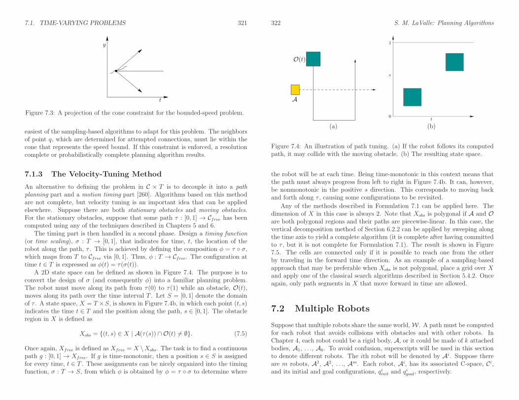
7.1. TIME-VARYING PROBLEMS 321
t
y
Figure 7.3: A projection of the cone constraint for the bounded-speed problem.
easiest of the sampling-based algorithms to adapt for this problem. The neighborsof point q, which are determined for attempted connections, must lie within thecone that represents the speed bound. If this constraint is enforced, a resolutioncomplete or probabilistically complete planning algorithm results.
7.1.3 The Velocity-Tuning Method
An alternative to defining the problem in C × T is to decouple it into a pathplanning part and a motion timing part [260]. Algorithms based on this methodare not complete, but velocity tuning is an important idea that can be appliedelsewhere. Suppose there are both stationary obstacles and moving obstacles.For the stationary obstacles, suppose that some path τ : [0, 1] → Cfree has beencomputed using any of the techniques described in Chapters 5 and 6.
The timing part is then handled in a second phase. Design a timing function(or time scaling), σ : T → [0, 1], that indicates for time, t, the location of therobot along the path, τ . This is achieved by defining the composition φ = τ σ,which maps from T to Cfree via [0, 1]. Thus, φ : T → Cfree. The configuration attime t ∈ T is expressed as φ(t) = τ(σ(t)).
A 2D state space can be defined as shown in Figure 7.4. The purpose is toconvert the design of σ (and consequently φ) into a familiar planning problem.The robot must move along its path from τ(0) to τ(1) while an obstacle, O(t),moves along its path over the time interval T . Let S = [0, 1] denote the domainof τ . A state space, X = T ×S, is shown in Figure 7.4b, in which each point (t, s)indicates the time t ∈ T and the position along the path, s ∈ [0, 1]. The obstacleregion in X is defined as
Xobs = (t, s) ∈ X | A(τ(s)) ∩ O(t) 6= ∅. (7.5)
Once again, Xfree is defined as Xfree = X \Xobs. The task is to find a continuouspath g : [0, 1] → Xfree. If g is time-monotonic, then a position s ∈ S is assignedfor every time, t ∈ T . These assignments can be nicely organized into the timingfunction, σ : T → S, from which φ is obtained by φ = τ σ to determine where
322 S. M. LaValle: Planning Algorithms
O(t)
A
t
1
0
s
(a) (b)
Figure 7.4: An illustration of path tuning. (a) If the robot follows its computedpath, it may collide with the moving obstacle. (b) The resulting state space.
the robot will be at each time. Being time-monotonic in this context means thatthe path must always progress from left to right in Figure 7.4b. It can, however,be nonmonotonic in the positive s direction. This corresponds to moving backand forth along τ , causing some configurations to be revisited.
Any of the methods described in Formulation 7.1 can be applied here. Thedimension of X in this case is always 2. Note that Xobs is polygonal if A and Oare both polygonal regions and their paths are piecewise-linear. In this case, thevertical decomposition method of Section 6.2.2 can be applied by sweeping alongthe time axis to yield a complete algorithm (it is complete after having committedto τ , but it is not complete for Formulation 7.1). The result is shown in Figure7.5. The cells are connected only if it is possible to reach one from the otherby traveling in the forward time direction. As an example of a sampling-basedapproach that may be preferable when Xobs is not polygonal, place a grid over Xand apply one of the classical search algorithms described in Section 5.4.2. Onceagain, only path segments in X that move forward in time are allowed.
7.2 Multiple Robots
Suppose that multiple robots share the same world,W . A path must be computedfor each robot that avoids collisions with obstacles and with other robots. InChapter 4, each robot could be a rigid body, A, or it could be made of k attachedbodies, A1, . . ., Ak. To avoid confusion, superscripts will be used in this sectionto denote different robots. The ith robot will be denoted by Ai. Suppose thereare m robots, A1, A2, . . ., Am. Each robot, Ai, has its associated C-space, Ci,and its initial and goal configurations, qiinit and q
igoal, respectively.
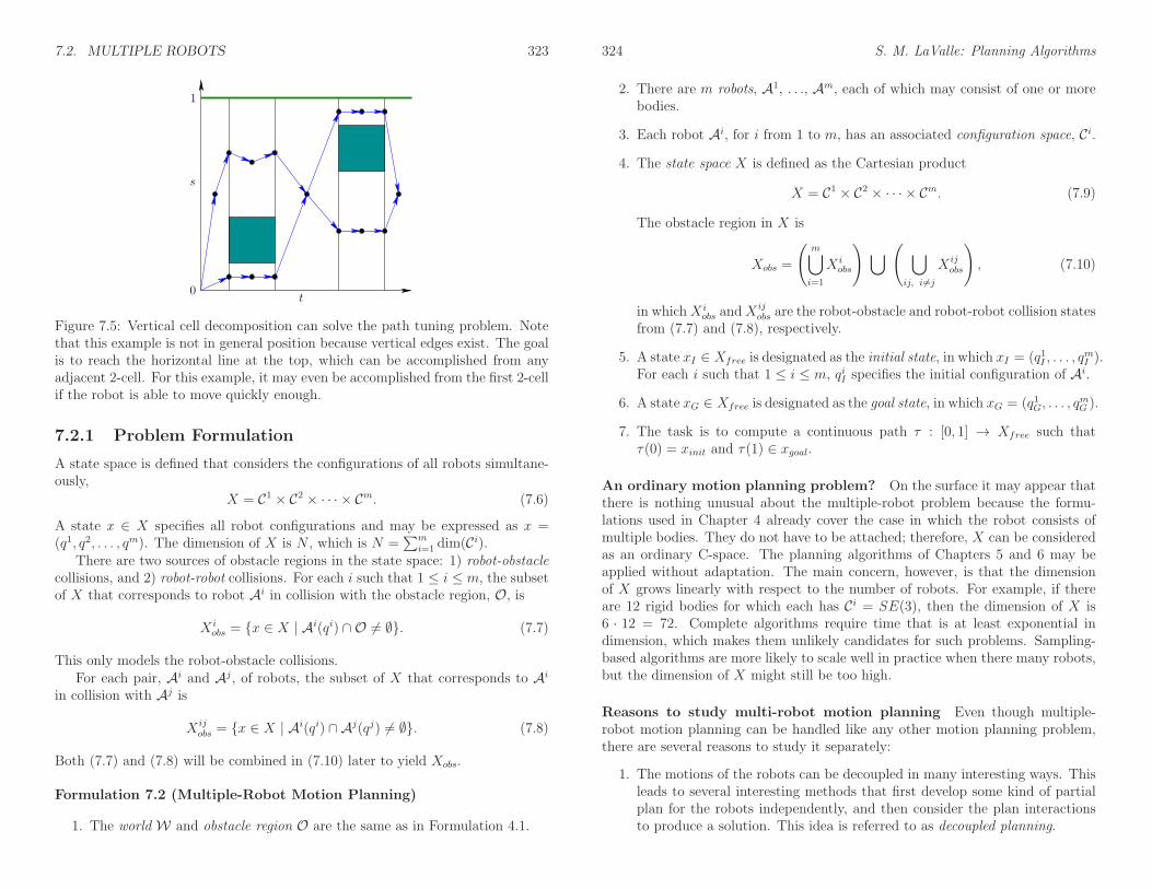
7.2. MULTIPLE ROBOTS 323
t
1
0
s
Figure 7.5: Vertical cell decomposition can solve the path tuning problem. Notethat this example is not in general position because vertical edges exist. The goalis to reach the horizontal line at the top, which can be accomplished from anyadjacent 2-cell. For this example, it may even be accomplished from the first 2-cellif the robot is able to move quickly enough.
7.2.1 Problem Formulation
A state space is defined that considers the configurations of all robots simultane-ously,
X = C1 × C2 × · · · × Cm. (7.6)
A state x ∈ X specifies all robot configurations and may be expressed as x =(q1, q2, . . . , qm). The dimension of X is N , which is N =
∑mi=1 dim(Ci).
There are two sources of obstacle regions in the state space: 1) robot-obstaclecollisions, and 2) robot-robot collisions. For each i such that 1 ≤ i ≤ m, the subsetof X that corresponds to robot Ai in collision with the obstacle region, O, is
X iobs = x ∈ X | Ai(qi) ∩ O 6= ∅. (7.7)
This only models the robot-obstacle collisions.For each pair, Ai and Aj, of robots, the subset of X that corresponds to Ai
in collision with Aj is
X ijobs = x ∈ X | Ai(qi) ∩ Aj(qj) 6= ∅. (7.8)
Both (7.7) and (7.8) will be combined in (7.10) later to yield Xobs.
Formulation 7.2 (Multiple-Robot Motion Planning)
1. The world W and obstacle region O are the same as in Formulation 4.1.
324 S. M. LaValle: Planning Algorithms
2. There are m robots, A1, . . ., Am, each of which may consist of one or morebodies.
3. Each robot Ai, for i from 1 to m, has an associated configuration space, Ci.
4. The state space X is defined as the Cartesian product
X = C1 × C2 × · · · × Cm. (7.9)
The obstacle region in X is
Xobs =
(
m⋃
i=1
X iobs
)
⋃
(
⋃
ij, i 6=j
X ijobs
)
, (7.10)
in whichX iobs andX
ijobs are the robot-obstacle and robot-robot collision states
from (7.7) and (7.8), respectively.
5. A state xI ∈ Xfree is designated as the initial state, in which xI = (q1I , . . . , qmI ).
For each i such that 1 ≤ i ≤ m, qiI specifies the initial configuration of Ai.
6. A state xG ∈ Xfree is designated as the goal state, in which xG = (q1G, . . . , qmG ).
7. The task is to compute a continuous path τ : [0, 1] → Xfree such thatτ(0) = xinit and τ(1) ∈ xgoal.
An ordinary motion planning problem? On the surface it may appear thatthere is nothing unusual about the multiple-robot problem because the formu-lations used in Chapter 4 already cover the case in which the robot consists ofmultiple bodies. They do not have to be attached; therefore, X can be consideredas an ordinary C-space. The planning algorithms of Chapters 5 and 6 may beapplied without adaptation. The main concern, however, is that the dimensionof X grows linearly with respect to the number of robots. For example, if thereare 12 rigid bodies for which each has Ci = SE(3), then the dimension of X is6 · 12 = 72. Complete algorithms require time that is at least exponential indimension, which makes them unlikely candidates for such problems. Sampling-based algorithms are more likely to scale well in practice when there many robots,but the dimension of X might still be too high.
Reasons to study multi-robot motion planning Even though multiple-robot motion planning can be handled like any other motion planning problem,there are several reasons to study it separately:
1. The motions of the robots can be decoupled in many interesting ways. Thisleads to several interesting methods that first develop some kind of partialplan for the robots independently, and then consider the plan interactionsto produce a solution. This idea is referred to as decoupled planning.

7.2. MULTIPLE ROBOTS 325
XX iXj X ijobs
Figure 7.6: The set X ijobs and its cylindrical structure on X.
2. The part of Xobs due to robot-robot collisions has a cylindrical structure,depicted in Figure 7.6, which can be exploited to make more efficient plan-ning algorithms. Each X ij
obs defined by (7.8) depends only on two robots. Apoint, x = (q1, . . . , qm), is in Xobs if there exists i, j such that 1 ≤ i, j ≤ mand Ai(qi) ∩Aj(qj) 6= ∅, regardless of the configurations of the other m− 2robots. For some decoupled methods, this even implies that Xobs can becompletely characterized by 2D projections, as depicted in Figure 7.9.
3. If optimality is important, then a unique set of issues arises for the caseof multiple robots. It is not a standard optimization problem because theperformance of each robot has to be optimized. There is no clear way tocombine these objectives into a single optimization problem without los-ing some critical information. It will be explained in Section 7.7.2 thatPareto optimality naturally arises as the appropriate notion of optimalityfor multiple-robot motion planning.
Assembly planning One important variant of multiple-robot motion planningis called assembly planning; recall from Section 1.2 its importance in applications.In automated manufacturing, many complicated objects are assembled step-by-step from individual parts. It is convenient for robots to manipulate the partsone-by-one to insert them into the proper locations (see Section 7.3.2). Imaginea collection of parts, each of which is interpreted as a robot, as shown in Figure7.7a. The goal is to assemble the parts into one coherent object, such as thatshown in Figure 7.7b. The problem is generally approached by starting withthe goal configuration, which is tightly constrained, and working outward. Theproblem formulation may allow that the parts touch, but their interiors cannotoverlap. In general, the assembly planning problem with arbitrarily many parts
326 S. M. LaValle: Planning Algorithms
A1 A2
A7
A3
A5
A6A4
A1
A2
A3
A4
A5
A6A7
(a) (b)
Figure 7.7: (a) A collection of pieces used to define an assembly planning problem;(b) assembly planning involves determining a sequence of motions that assemblesthe parts. The object shown here is assembled from the parts.
is NP-hard. Polynomial-time algorithms have been developed in several specialcases. For the case in which parts can be removed by a sequence of straight-linepaths, a polynomial-time algorithm is given in [476, 477].
7.2.2 Decoupled planning
Decoupled approaches first design motions for the robots while ignoring robot-robot interactions. Once these interactions are considered, the choices availableto each robot are already constrained by the designed motions. If a problem arises,these approaches are typically unable to reverse their commitments. Therefore,completeness is lost. Nevertheless, decoupled approaches are quite practical, andin some cases completeness can be recovered.
Prioritized planning A straightforward approach to decoupled planning is tosort the robots by priority and plan for higher priority robots first [166, 466]. Lowerpriority robots plan by viewing the higher priority robots as moving obstacles.Suppose the robots are sorted as A1, . . ., Am, in which A1 has the highest priority.
Assume that collision-free paths, τi : [0, 1] → Cifree, have been computed for ifrom 1 to n. The prioritized planning approach proceeds inductively as follows:
Base case: Use any motion planning algorithm from Chapters 5 and 6 tocompute a collision-free path, τ1 : [0, 1] → C1free for A1. Compute a timingfunction, σ1, for τ1, to yield φ1 = τ1 σ1 : T → C1free.
Inductive step: Suppose that φ1, . . ., φi−1 have been designed for A1, . . .,Ai−1, and that these functions avoid robot-robot collisions between any ofthe first i − 1 robots. Formulate the first i − 1 robots as moving obstaclesin W . For each t ∈ T and j ∈ 1, . . . , i − 1, the configuration qj of eachAj is φj(t). This yields Aj(φj(t)) ⊂ W , which can be considered as a subsetof the obstacle O(t). Design a path, τi, and timing function, σi, using anyof the time-varying motion planning methods from Section 7.1 and formφi = τi σi.
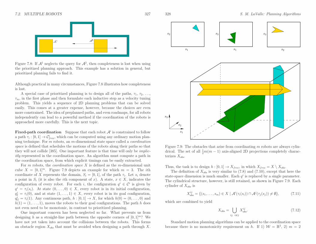
7.2. MULTIPLE ROBOTS 327
A2 A1
Figure 7.8: If A1 neglects the query for A2, then completeness is lost when usingthe prioritized planning approach. This example has a solution in general, butprioritized planning fails to find it.
Although practical in many circumstances, Figure 7.8 illustrates how completenessis lost.
A special case of prioritized planning is to design all of the paths, τ1, τ2, . . .,τm, in the first phase and then formulate each inductive step as a velocity tuningproblem. This yields a sequence of 2D planning problems that can be solvedeasily. This comes at a greater expense, however, because the choices are evenmore constrained. The idea of preplanned paths, and even roadmaps, for all robotsindependently can lead to a powerful method if the coordination of the robots isapproached more carefully. This is the next topic.
Fixed-path coordination Suppose that each robot Ai is constrained to followa path τi : [0, 1]→ Cifree, which can be computed using any ordinary motion plan-ning technique. For m robots, an m-dimensional state space called a coordinationspace is defined that schedules the motions of the robots along their paths so thatthey will not collide [385]. One important feature is that time will only be implic-itly represented in the coordination space. An algorithm must compute a path inthe coordination space, from which explicit timings can be easily extracted.
For m robots, the coordination space X is defined as the m-dimensional unitcube X = [0, 1]m. Figure 7.9 depicts an example for which m = 3. The ithcoordinate of X represents the domain, Si = [0, 1], of the path τi. Let si denotea point in Si (it is also the ith component of x). A state, x ∈ X, indicates theconfiguration of every robot. For each i, the configuration qi ∈ Ci is given byqi = τi(si). At state (0, . . . , 0) ∈ X, every robot is in its initial configuration,qiI = τi(0), and at state (1, . . . , 1) ∈ X, every robot is in its goal configuration,qiG = τi(1). Any continuous path, h : [0, 1] → X, for which h(0) = (0, . . . , 0) andh(1) = (1, . . . , 1), moves the robots to their goal configurations. The path h doesnot even need to be monotonic, in contrast to prioritized planning.
One important concern has been neglected so far. What prevents us fromdesigning h as a straight-line path between the opposite corners of [0, 1]m? Wehave not yet taken into account the collisions between the robots. This formsan obstacle region Xobs that must be avoided when designing a path through X.
328 S. M. LaValle: Planning Algorithms
s1
s2
s3
s1
s2
s1
s3
s2
s3
Figure 7.9: The obstacles that arise from coordinating m robots are always cylin-drical. The set of all 1
2m(m − 1) axis-aligned 2D projections completely charac-
terizes Xobs.
Thus, the task is to design h : [0, 1]→ Xfree, in which Xfree = X \Xobs.The definition of Xobs is very similar to (7.8) and (7.10), except that here the
state-space dimension is much smaller. Each qi is replaced by a single parameter.The cylindrical structure, however, is still retained, as shown in Figure 7.9. Eachcylinder of Xobs is
X ijobs = (s1, . . . , sm) ∈ X | Ai(τi(si)) ∩ Aj(τj(sj)) 6= ∅, (7.11)
which are combined to yield
Xobs =⋃
ij, i 6=j
X ijobs. (7.12)
Standard motion planning algorithms can be applied to the coordination spacebecause there is no monotonicity requirement on h. If 1) W = R2, 2) m = 2

7.2. MULTIPLE ROBOTS 329
(two robots), 3) the obstacles and robots are polygonal, and 4) the paths, τi, arepiecewise-linear, then Xobs is a polygonal region in X. This enables the methodsof Section 6.2, for a polygonal Cobs, to directly apply after the representation ofXobs is explicitly constructed. Form > 2, the multi-dimensional version of verticalcell decomposition given for m = 3 in Section 6.3.3 can be applied. For generalcoordination problems, cylindrical algebraic decomposition or Canny’s roadmapalgorithm can be applied. For the problem of robots in W = R2 that eithertranslate or move along circular paths, a resolution complete planning methodbased on the exact determination of Xobs using special collision detection methodsis given in [441].
For very challenging coordination problems, sampling-based solutions mayyield practical solutions. Perhaps one of the simplest solutions is to place agrid over X and adapt the classical search algorithms, as described in Section5.4.2 [309, 385]. Other possibilities include using the RDTs of Section 5.5 or, ifthe multiple-query framework is appropriate, then the sampling-based roadmapmethods of 5.6 are suitable. Methods for validating the path segments, whichwere covered in Section 5.3.4, can be adapted without trouble to the case of co-ordination spaces.
Thus far, the particular speeds of the robots have been neglected. For expla-nation purposes, consider the case of m = 2. Moving vertically or horizontally inX holds one robot fixed while the other moves at some maximum speed. Movingdiagonally in X moves both robots, and their relative speeds depend on the slopeof the path. To carefully regulate these speeds, it may be necessary to reparam-eterize the paths by distance. In this case each axis of X represents the distancetraveled, instead of [0, 1].
Fixed-roadmap coordination The fixed-path coordination approach still maynot solve the problem in Figure 7.8 if the paths are designed independently. For-tunately, fixed-path coordination can be extended to enable each robot to moveover a roadmap or topological graph. This still yields a coordination space thathas only one dimension per robot, and the resulting planning methods are muchcloser to being complete, assuming each robot utilizes a roadmap that has manyalternative paths. There is also motivation to study this problem by itself becauseof automated guided vehicles (AGVs), which often move in factories on a networkof predetermined paths. In this case, coordinating the robots is the planningproblem, as opposed to being a simplification of Formulation 7.2.
One way to obtain completeness for Formulation 7.2 is to design the indepen-dent roadmaps so that each robot has its own garage configuration. The conditionsfor a configuration, qi, to be a garage for Ai are 1) while at configuration qi, it isimpossible for any other robots to collide with it (i.e., in all coordination states forwhich the ith coordinate is qi, no collision occurs); and 2) qi is always reachableby Ai from xI . If each robot has a roadmap and a garage, and if the planningmethod for X is complete, then the overall planning algorithm is complete. If the
330 S. M. LaValle: Planning Algorithms
planning method in X uses some weaker notion of completeness, then this is alsomaintained. For example, a resolution complete planner for X yields a resolutioncomplete approach to the problem in Formulation 7.2.
Cube complex How is the coordination space represented when there are mul-tiple paths for each robot? It turns out that a cube complex is obtained, which isa special kind of singular complex (recall from Section 6.3.1). The coordinationspace for m fixed paths can be considered as a singular m-simplex. For example,the problem in Figure 7.9 can be considered as a singular 3-simplex, [0, 1]3 → X.In Section 6.3.1, the domain of a k-simplex was defined using Bk, a k-dimensionalball; however, a cube, [0, 1]k, also works because Bk and [0, 1]k are homeomorphic.
For a topological space, X, let a k-cube (which is also a singular k-simplex),k, be a continuous mapping σ : [0, 1]k → X. A cube complex is obtained byconnecting together k-cubes of different dimensions. Every k-cube for k ≥ 1 has2k faces, which are (k − 1)-cubes that are obtained as follows. Let (s1, . . . , sk)denote a point in [0, 1]k. For each i ∈ 1, . . . , k, one face is obtained by settingsi = 0 and another is obtained by setting si = 1.
The cubes must fit together nicely, much in the same way that the simplexesof a simplicial complex were required to fit together. To be a cube complex, Kmust be a collection of simplexes that satisfy the following requirements:
1. Any face, k−1, of a cube k ∈ K is also in K.
2. The intersection of the images of any two k-cubes k,′k ∈ K, is either
empty or there exists some cube, i ∈ K for i < k, which is a common faceof both k and
′k.
Let Gi denote a topological graph (which may also be a roadmap) for robotAi. The graph edges are paths of the form τ : [0, 1] → Cifree. Before coveringformal definitions of the resulting complex, consider Figure 7.10a, in which A1
moves along three paths connected in a “T” junction and A2 moves along onepath. In this case, three 2D fixed-path coordination spaces are attached togetheralong one common edge, as shown in Figure 7.10b. The resulting cube complex isdefined by three 2-cubes (i.e., squares), one 1-cube (i.e., line segment), and eight0-cubes (i.e., corner points).
Now suppose more generally that there are two robots, A1 and A2, with asso-ciated topological graphs, G1(V1, E1) and G2(V2, E2), respectively. Suppose that Gand G2 have n1 and n2 edges, respectively. A 2D cube complex, K, is obtained asfollows. Let τi denote the ith path of G1, and let σj denote the jth path of G2. A2-cube (square) exists in K for every way to select an edge from each graph. Thus,there are n1n2 2-cubes, one for each pair (τi, σj), such that τi ∈ E1 and σj ∈ E2.The 1-cubes are generated for pairs of the form (vi, σj) for vi ∈ V1 and σj ∈ E2,or (τi, vj) for τi ∈ E1 and vj ∈ V2. The 0-cubes (corner points) are reached foreach pair (vi, vj) such that vi ∈ V1 and vj ∈ V2.
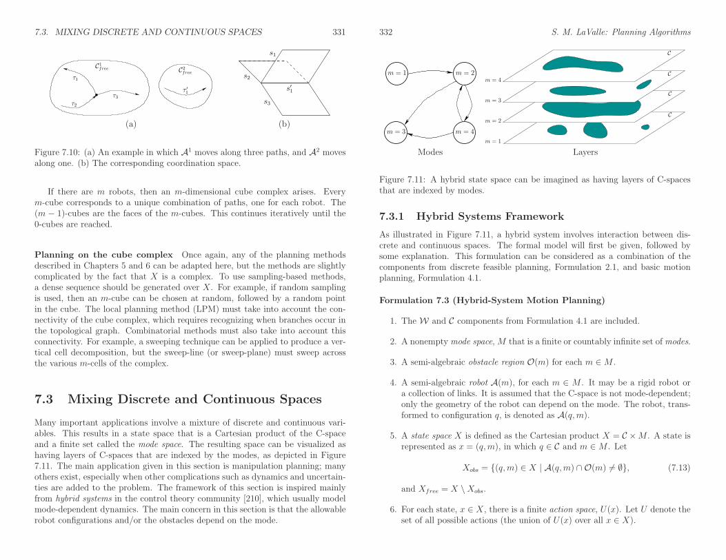
7.3. MIXING DISCRETE AND CONTINUOUS SPACES 331
τ2
τ1
C1free
τ3
C2free
τ ′1
s3
s′1
s2
s1
(a) (b)
Figure 7.10: (a) An example in which A1 moves along three paths, and A2 movesalong one. (b) The corresponding coordination space.
If there are m robots, then an m-dimensional cube complex arises. Everym-cube corresponds to a unique combination of paths, one for each robot. The(m − 1)-cubes are the faces of the m-cubes. This continues iteratively until the0-cubes are reached.
Planning on the cube complex Once again, any of the planning methodsdescribed in Chapters 5 and 6 can be adapted here, but the methods are slightlycomplicated by the fact that X is a complex. To use sampling-based methods,a dense sequence should be generated over X. For example, if random samplingis used, then an m-cube can be chosen at random, followed by a random pointin the cube. The local planning method (LPM) must take into account the con-nectivity of the cube complex, which requires recognizing when branches occur inthe topological graph. Combinatorial methods must also take into account thisconnectivity. For example, a sweeping technique can be applied to produce a ver-tical cell decomposition, but the sweep-line (or sweep-plane) must sweep acrossthe various m-cells of the complex.
7.3 Mixing Discrete and Continuous Spaces
Many important applications involve a mixture of discrete and continuous vari-ables. This results in a state space that is a Cartesian product of the C-spaceand a finite set called the mode space. The resulting space can be visualized ashaving layers of C-spaces that are indexed by the modes, as depicted in Figure7.11. The main application given in this section is manipulation planning; manyothers exist, especially when other complications such as dynamics and uncertain-ties are added to the problem. The framework of this section is inspired mainlyfrom hybrid systems in the control theory community [210], which usually modelmode-dependent dynamics. The main concern in this section is that the allowablerobot configurations and/or the obstacles depend on the mode.
332 S. M. LaValle: Planning Algorithms
m = 4
m = 1 m = 2
m = 3
m = 4
m = 3
m = 2
m = 1
C
C
C
C
Modes Layers
Figure 7.11: A hybrid state space can be imagined as having layers of C-spacesthat are indexed by modes.
7.3.1 Hybrid Systems Framework
As illustrated in Figure 7.11, a hybrid system involves interaction between dis-crete and continuous spaces. The formal model will first be given, followed bysome explanation. This formulation can be considered as a combination of thecomponents from discrete feasible planning, Formulation 2.1, and basic motionplanning, Formulation 4.1.
Formulation 7.3 (Hybrid-System Motion Planning)
1. The W and C components from Formulation 4.1 are included.
2. A nonempty mode space,M that is a finite or countably infinite set of modes.
3. A semi-algebraic obstacle region O(m) for each m ∈M .
4. A semi-algebraic robot A(m), for each m ∈ M . It may be a rigid robot ora collection of links. It is assumed that the C-space is not mode-dependent;only the geometry of the robot can depend on the mode. The robot, trans-formed to configuration q, is denoted as A(q,m).
5. A state space X is defined as the Cartesian product X = C ×M . A state isrepresented as x = (q,m), in which q ∈ C and m ∈M . Let
Xobs = (q,m) ∈ X | A(q,m) ∩ O(m) 6= ∅, (7.13)
and Xfree = X \Xobs.
6. For each state, x ∈ X, there is a finite action space, U(x). Let U denote theset of all possible actions (the union of U(x) over all x ∈ X).

7.3. MIXING DISCRETE AND CONTINUOUS SPACES 333
7. There is a mode transition function fm that produces a mode, fm(x, u) ∈M ,for every x ∈ X and u ∈ U(x). It is assumed that fm is defined in a way thatdoes not produce race conditions (oscillations of modes within an instant oftime). This means that if q is fixed, the mode can change at most once. Itthen remains constant and can change only if q is changed.
8. There is a state transition function, f , that is derived from fm by changingthe mode and holding the configuration fixed. Thus, f(x, u) = (q, fm(x, u)).
9. A configuration xI ∈ Xfree is designated as the initial state.
10. A set XG ∈ Xfree is designated as the goal region. A region is defined insteadof a point to facilitate the specification of a goal configuration that does notdepend on the final mode.
11. An algorithm must compute a (continuous) path τ : [0, 1] → Xfree and anaction trajectory σ : [0, 1] → U such that τ(0) = xI and τ(1) ∈ XG, or thealgorithm correctly reports that such a combination of a path and an actiontrajectory does not exist.
The obstacle region and robot may or may not be mode-dependent, dependingon the problem. Examples of each will be given shortly. Changes in the modedepend on the action taken by the robot. From most states, it is usually assumedthat a “do nothing” action exists, which leaves the mode unchanged. From certainstates, the robot may select an action that changes the mode as desired. Aninteresting degenerate case exists in which there is only a single action available.This means that the robot has no control over the mode from that state. If therobot arrives in such a state, a mode change could unavoidably occur.
The solution requirement is somewhat more complicated because both a pathand an action trajectory need to be specified. It is insufficient to specify a pathbecause it is important to know what action was applied to induce the correctmode transitions. Therefore, σ indicates when these occur. Note that τ and σare closely coupled; one cannot simply associate any σ with a path τ ; it mustcorrespond to the actions required to generate τ .
Example 7.2 (The Power of the Portiernia) In this example, a robot, A, ismodeled as a square that translates in W = R2. Therefore, C = R2. The obstacleregion in W is mode-dependent because of two doors, which are numbered “1”and “2” in Figure 7.12a. In the upper left sits the portiernia,2 which is able togive a key to the robot, if the robot is in a configuration as shown in Figure 7.12b.The portiernia only trusts the robot with one key at a time, which may be eitherfor Door 1 or Door 2. The robot can return a key by revisiting the portiernia. Asshown in Figures 7.12c and 7.12d, the robot can open a door by making contactwith it, as long as it holds the correct key.
2This is a place where people guard the keys at some public facilities in Poland.
334 S. M. LaValle: Planning Algorithms
1
2A
1
2
A
(a) (b)
1
2
A
2
A
(c) (d)
Figure 7.12: In the upper left (at the portiernia), the robot can pick up and dropoff keys that open one of two doors. If the robot contacts a door while holdingthe correct key, then it opens.
The set, M , of modes needs to encode which key, if any, the robot holds, andit must also encode the status of the doors. The robot may have: 1) the key toDoor 1; 2) the key to Door 2; or 3) no keys. The doors may have the status: 1)both open; 2) Door 1 open, Door 2 closed; 3) Door 1 closed, Door 2 open; or 4)both closed. Considering keys and doors in combination yields 12 possible modes.
If the robot is at a portiernia configuration as shown in Figure 7.12b, then itsavailable actions correspond to different ways to pick up and drop off keys. Forexample, if the robot is holding the key to Door 1, it can drop it off and pickup the key to Door 2. This changes the mode, but the door status and robotconfiguration must remain unchanged when f is applied. The other locations inwhich the robot may change the mode are when it comes in contact with Door 1or Door 2. The mode changes only if the robot is holding the proper key. In allother configurations, the robot only has a single action (i.e., no choice), whichkeeps the mode fixed.
The task is to reach the configuration shown in the lower right with dashed

7.3. MIXING DISCRETE AND CONTINUOUS SPACES 335
lines. The problem is solved by: 1) picking up the key for Door 1 at the portiernia;2) opening Door 1; 3) swapping the key at the portiernia to obtain the key forDoor 2; or 4) entering the innermost room to reach the goal configuration. As afinal condition, we might want to require that the robot returns the key to theportiernia.
A
A
Elongated
Compressed
Figure 7.13: An example in which the robot must reconfigure itself to solve theproblem. There are two modes: elongated and compressed.
A A
Elongated mode Compressed mode
Figure 7.14: When the robot reconfigures itself, Cfree(m) changes, enabling theproblem to be solved.
Example 7.2 allows the robot to change the obstacles in O. The next exampleinvolves a robot that can change its shape. This is an illustrative example ofa reconfigurable robot. The study of such robots has become a popular topic ofresearch [112, 196, 290, 484]; the reconfiguration possibilities in that research areaare much more complicated than the simple example considered here.
Example 7.3 (Reconfigurable Robot) To solve the problem shown in Figure7.13, the robot must change its shape. There are two possible shapes, whichcorrespond directly to the modes: elongated and compressed. Examples of eachare shown in the figure. Figure 7.14 shows how Cfree(m) appears for each of thetwo modes. Suppose the robot starts initially from the left while in the elongatedmode and must travel to the last room on the right. This problem must be solvedby 1) reconfiguring the robot into the compressed mode; 2) passing through the
336 S. M. LaValle: Planning Algorithms
corridor into the center; 3) reconfiguring the robot into the elongated mode; and4) passing through the corridor to the rightmost room. The robot has actionsthat directly change the mode by reconfiguring itself. To make the problem moreinteresting, we could require the robot to reconfigure itself in specific locations(e.g., where there is enough clearance, or possibly at a location where anotherrobot can assist it).
The examples presented so far barely scratch the surface on the possible hybridmotion planning problems that can be defined. Many such problems can arise, forexample, in the context making automated video game characters or digital actors.To solve these problems, standard motion planning algorithms can be adapted ifthey are given information about how to change the modes. Locations in Xfrom which the mode can be changed may be expressed as subgoals. Much of theplanning effort should then be focused on attempting to change modes, in additionto trying to directly reach the goal. Applying sampling-based methods requiresthe definition of a metric on X that accounts for both changes in the mode and theconfiguration. A wide variety of hybrid problems can be formulated, ranging fromthose that are impossible to solve in practice to those that are straightforwardextensions of standard motion planning. In general, the hybrid motion planningmodel is useful for formulating a hierarchical approach, as described in Section1.4. One particularly interesting class of problems that fit this model, for whichsuccessful algorithms have been developed, will be covered next.
7.3.2 Manipulation Planning
This section presents an overview of manipulation planning; the concepts ex-plained here are mainly due to [11, 12]. Returning to Example 7.2, imagine thatthe robot must carry a key that is so large that it changes the connectivity ofCfree. For the manipulation planning problem, the robot is called a manipula-tor, which interacts with a part. In some configurations it is able to grasp thepart and move it to other locations in the environment. The manipulation taskusually requires moving the part to a specified location in W , without particularregard as to how the manipulator can accomplish the task. The model consideredhere greatly simplifies the problems of grasping, stability, friction, mechanics, anduncertainties and instead focuses on the geometric aspects (some of these issueswill be addressed in Section 12.5). For a thorough introduction to these otherimportant aspects of manipulation planning, see [352]; see also Sections 13.1.3and 12.5.
Admissible configurations Assume that W , O, and A from Formulation 4.1are used. For manipulation planning, A is called the manipulator, and let Carefer to the manipulator configuration space. Let P denote a part, which is arigid body modeled in terms of geometric primitives, as described in Section 3.1.It is assumed that P is allowed to undergo rigid-body transformations and will

7.3. MIXING DISCRETE AND CONTINUOUS SPACES 337
therefore have its own part configuration space, Cp = SE(2) or Cp = SE(3). Letqp ∈ Cp denote a part configuration. The transformed part model is denoted asP(qp).
O
A(qa)
O
P(qp) P(qp)
A(qa)
q ∈ Caobs q ∈ Cpobs q ∈ Capobs
P(q p)
A(q a)
P(qp) P(qp)
A(qa)
q ∈ Cgr q ∈ Csta q ∈ Ctra
Figure 7.15: Examples of several important subsets of C for manipulation plan-ning.
The combined configuration space, C, is defined as the Cartesian product
C = Ca × Cp, (7.14)
in which each configuration q ∈ C is of the form q = (qa, qp). The first step isto remove all configurations that must be avoided. Parts of Figure 7.15 showexamples of these sets. Configurations for which the manipulator collides withobstacles are
Caobs = (qa, qp) ∈ C | A(qa) ∩ O 6= ∅. (7.15)
The next logical step is to remove configurations for which the part collides withobstacles. It will make sense to allow the part to “touch” the obstacles. Forexample, this could model a part sitting on a table. Therefore, let
Cpobs = (qa, qp) ∈ C | int(P(qp)) ∩ O 6= ∅ (7.16)
denote the open set for which the interior of the part intersects O. Certainly, ifthe part penetrates O, then the configuration should be avoided.
338 S. M. LaValle: Planning Algorithms
Consider C \(Caobs∪Cpobs). The configurations that remain ensure that the robotand part do not inappropriately collide with O. Next consider the interactionbetween A and P . The manipulator must be allowed to touch the part, butpenetration is once again not allowed. Therefore, let
Capobs = (qa, qp) ∈ C | A(qa) ∩ int(P(qp)) 6= ∅. (7.17)
Removing all of these bad configurations yields
Cadm = C \ (Caobs ∪ Cpobs ∪ Capobs), (7.18)
which is called the set of admissible configurations.
Stable and grasped configurations Two important subsets of Cadm are usedin the manipulation planning problem. See Figure 7.15. Let Cpsta denote the set ofstable part configurations, which are configurations at which the part can safelyrest without any forces being applied by the manipulator. This means that a partcannot, for example, float in the air. It also cannot be in a configuration fromwhich it might fall. The particular stable configurations depend on propertiessuch as the part geometry, friction, mass distribution, and so on. These issuesare not considered here. From this, let Csta ⊆ Cadm be the corresponding stableconfigurations, defined as
Csta = (qa, qp) ∈ Cadm | qp ∈ Cpsta. (7.19)
The other important subset of Cadm is the set of all configurations in which therobot is grasping the part (and is capable of carrying it, if necessary). Letthis denote the grasped configurations, denoted by Cgr ⊆ Cadm. For every con-figuration, (qa, qp) ∈ Cgr, the manipulator touches the part. This means thatA(qa) ∩ P(qp) 6= ∅ (penetration is still not allowed because Cgr ⊆ Cadm). In gen-eral, many configurations at which A(qa) contacts P(qp) will not necessarily bein Cgr. The conditions for a point to lie in Cgr depend on the particular charac-teristics of the manipulator, the part, and the contact surface between them. Forexample, a typical manipulator would not be able to pick up a block by makingcontact with only one corner of it. This level of detail is not defined here; see [352]for more information about grasping.
We must always ensure that either x ∈ Csta or x ∈ Cgr. Therefore, letCfree = Csta ∪ Cgr, to reflect the subset of Cadm that is permissible for manip-ulation planning.
The mode space, M , contains two modes, which are named the transit modeand the transfer mode. In the transit mode, the manipulator is not carrying thepart, which requires that q ∈ Csta. In the transfer mode, the manipulator carriesthe part, which requires that q ∈ Cgr. Based on these simple conditions, the onlyway the mode can change is if q ∈ Csta ∩ Cgr. Therefore, the manipulator has twoavailable actions only when it is in these configurations. In all other configurations
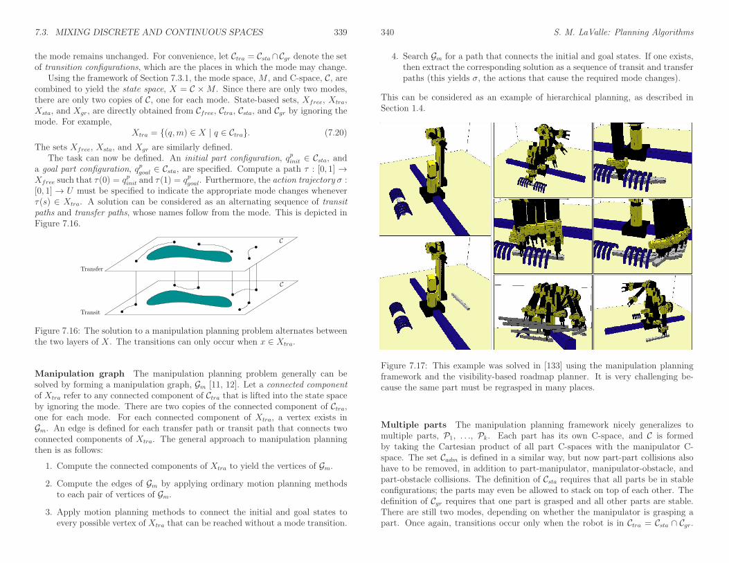
7.3. MIXING DISCRETE AND CONTINUOUS SPACES 339
the mode remains unchanged. For convenience, let Ctra = Csta∩Cgr denote the setof transition configurations, which are the places in which the mode may change.
Using the framework of Section 7.3.1, the mode space, M , and C-space, C, arecombined to yield the state space, X = C ×M . Since there are only two modes,there are only two copies of C, one for each mode. State-based sets, Xfree, Xtra,Xsta, and Xgr, are directly obtained from Cfree, Ctra, Csta, and Cgr by ignoring themode. For example,
Xtra = (q,m) ∈ X | q ∈ Ctra. (7.20)
The sets Xfree, Xsta, and Xgr are similarly defined.The task can now be defined. An initial part configuration, qpinit ∈ Csta, and
a goal part configuration, qpgoal ∈ Csta, are specified. Compute a path τ : [0, 1] →Xfree such that τ(0) = qpinit and τ(1) = qpgoal. Furthermore, the action trajectory σ :[0, 1] → U must be specified to indicate the appropriate mode changes wheneverτ(s) ∈ Xtra. A solution can be considered as an alternating sequence of transitpaths and transfer paths, whose names follow from the mode. This is depicted inFigure 7.16.
Transfer
Transit
C
C
Figure 7.16: The solution to a manipulation planning problem alternates betweenthe two layers of X. The transitions can only occur when x ∈ Xtra.
Manipulation graph The manipulation planning problem generally can besolved by forming a manipulation graph, Gm [11, 12]. Let a connected componentof Xtra refer to any connected component of Ctra that is lifted into the state spaceby ignoring the mode. There are two copies of the connected component of Ctra,one for each mode. For each connected component of Xtra, a vertex exists inGm. An edge is defined for each transfer path or transit path that connects twoconnected components of Xtra. The general approach to manipulation planningthen is as follows:
1. Compute the connected components of Xtra to yield the vertices of Gm.
2. Compute the edges of Gm by applying ordinary motion planning methodsto each pair of vertices of Gm.
3. Apply motion planning methods to connect the initial and goal states toevery possible vertex of Xtra that can be reached without a mode transition.
340 S. M. LaValle: Planning Algorithms
4. Search Gm for a path that connects the initial and goal states. If one exists,then extract the corresponding solution as a sequence of transit and transferpaths (this yields σ, the actions that cause the required mode changes).
This can be considered as an example of hierarchical planning, as described inSection 1.4.
Figure 7.17: This example was solved in [133] using the manipulation planningframework and the visibility-based roadmap planner. It is very challenging be-cause the same part must be regrasped in many places.
Multiple parts The manipulation planning framework nicely generalizes tomultiple parts, P1, . . ., Pk. Each part has its own C-space, and C is formedby taking the Cartesian product of all part C-spaces with the manipulator C-space. The set Cadm is defined in a similar way, but now part-part collisions alsohave to be removed, in addition to part-manipulator, manipulator-obstacle, andpart-obstacle collisions. The definition of Csta requires that all parts be in stableconfigurations; the parts may even be allowed to stack on top of each other. Thedefinition of Cgr requires that one part is grasped and all other parts are stable.There are still two modes, depending on whether the manipulator is grasping apart. Once again, transitions occur only when the robot is in Ctra = Csta ∩ Cgr.

7.4. PLANNING FOR CLOSED KINEMATIC CHAINS 341
Figure 7.18: This manipulation planning example was solved in [452] and involves90 movable pieces of furniture. Some of them must be dragged out of the way tosolve the problem. Paths for two different queries are shown.
The task involves moving each part from one configuration to another. This isachieved once again by defining a manipulation graph and obtaining a sequenceof transit paths (in which no parts move) and transfer paths (in which one part iscarried and all other parts are fixed). Challenging manipulation problems solvedby motion planning algorithms are shown in Figures 7.17 and 7.18.
Other generalizations are possible. A generalization to k robots would lead to2k modes, in which each mode indicates whether each robot is grasping the part.Multiple robots could even grasp the same object. Another generalization couldallow a single robot to grasp more than one object.
7.4 Planning for Closed Kinematic Chains
This section continues where Section 4.4 left off. The subspace of C that resultsfrom maintaining kinematic closure was defined and illustrated through some ex-
342 S. M. LaValle: Planning Algorithms
amples. Planning in this context requires that paths remain on a lower dimensionalvariety for which a parameterization is not available. Many important applica-tions require motion planning while maintaining these constraints. For example,consider a manipulation problem that involves multiple manipulators graspingthe same object, which forms a closed loop as shown in Figure 7.19. A loopexists because both manipulators are attached to the ground, which may itselfbe considered as a link. The development of virtual actors for movies and videogames also involves related manipulation problems. Loops also arise in this con-text when more than one human limb is touching a fixed surface (e.g., two feet onthe ground). A class of robots called parallel manipulators are intentionally de-signed with internal closed loops [360]. For example, consider the Stewart-Goughplatform [208, 451] illustrated in Figure 7.20. The lengths of each of the six arms,A1, . . ., A6, can be independently varied while they remain attached via sphericaljoints to the ground and to the platform, which is A7. Each arm can actually beimagined as two links that are connected by a prismatic joint. Due to the totalof 6 degrees of freedom introduced by the variable lengths, the platform actu-ally achieves the full 6 degrees of freedom (hence, some six-dimensional region inSE(3) is obtained for A7). Planning the motion of the Stewart-Gough platform,or robots that are based on the platform (the robot shown in Figure 7.27 uses astack of several of these mechanisms), requires handling many closure constraintsthat must be maintained simultaneously. Another application is computationalbiology, in which the C-space of molecules is searched, many of which are derivedfrom molecules that have closed, flexible chains of bonds [134].
7.4.1 Adaptation of Motion Planning Algorithms
All of the components from the general motion planning problem of Formulation4.1 are included: W , O, A1, . . ., Am, C, qI , and qG. It is assumed that the robotis a collection of r links that are possibly attached in loops.
It is assumed in this section that C = Rn. If this is not satisfactory, there aretwo ways to overcome the assumption. The first is to represent SO(2) and SO(3)as S1 and S3, respectively, and include the circle or sphere equation as part of theconstraints considered here. This avoids the topology problems. The other optionis to abandon the restriction of using Rn and instead use a parameterization of Cthat is of the appropriate dimension. To perform calculus on such manifolds, asmooth structure is required, which is introduced in Section 8.3.2. In the presenta-tion here, however, vector calculus on Rn is sufficient, which intentionally avoidsthese extra technicalities.
Closure constraints The closure constraints introduced in Section 4.4 can besummarized as follows. There is a set, P , of polynomials f1, . . ., fk that belongto Q[q1, . . . , qn] and express the constraints for particular points on the links ofthe robot. The determination of these is detailed in Section 4.4.3. As mentioned

7.4. PLANNING FOR CLOSED KINEMATIC CHAINS 343
Figure 7.19: Two or more manipulators manipulating the same object causesclosed kinematic chains. Each black disc corresponds to a revolute joint.
previously, polynomials that force points to lie on a circle or sphere in the case ofrotations may also be included in P .
Let n denote the dimension of C. The closure space is defined as
Cclo = q ∈ C | ∀fi ∈ P , fi(q1, . . . , qn) = 0, (7.21)
which is an m-dimensional subspace of C that corresponds to all configurationsthat satisfy the closure constants. The obstacle set must also be taken into ac-count. Once again, Cobs and Cfree are defined using (4.34). The feasible space isdefined as Cfea = Cclo ∩ Cfree, which are the configurations that satisfy closureconstraints and avoid collisions.
The motion planning problem is to find a path τ : [0, 1]→ Cfea such that τ(0) =qI and τ(1) = qG. The new challenge is that there is no explicit parameterizationof Cfea, which is further complicated by the fact that m < n (recall that m is thedimension of Cclo).
Combinatorial methods Since the constraints are expressed with polynomi-als, it may not be surprising that the computational algebraic geometry methodsof Section 6.4 can solve the general motion planning problem with closed kinematicchains. Either cylindrical algebraic decomposition or Canny’s roadmap algorithmmay be applied. As mentioned in Section 6.5.3, an adaptation of the roadmapalgorithm that is optimized for problems in which m < n is given in [52].
344 S. M. LaValle: Planning Algorithms
A5
A6
A4
A3A2
A1
A7
Figure 7.20: An illustration of the Stewart-Gough platform (adapted from a figuremade by Frank Sottile).
Sampling-based methods Most of the methods of Chapter 5 are not easy toadapt because they require sampling in Cfea, for which a parameterization doesnot exist. If points in a bounded region of Rn are chosen at random, the proba-bility is zero that a point on Cfea will be obtained. Some incremental samplingand searching methods can, however, be adapted by the construction of a localplanning method (LPM) that is suited for problems with closure constraints. Thesampling-based roadmap methods require many samples to be generated directlyon Cfea. Section 7.4.2 presents some techniques that can be used to generatesuch samples for certain classes of problems, enabling the development of efficientsampling-based planners and also improving the efficiency of incremental searchplanners. Before covering these techniques, we first present a method that leadsto a more general sampling-based planner and is easier to implement. However, ifdesigned well, planners based on the techniques of Section 7.4.2 are more efficient.
Now consider adapting the RDT of Section 5.5 to work for problems withclosure constraints. Similar adaptations may be possible for other incrementalsampling and searching methods covered in Section 5.4, such as the randomizedpotential field planner. A dense sampling sequence, α, is generated over a boundedn-dimensional subset of Rn, such as a rectangle or sphere, as shown in Figure 7.21.
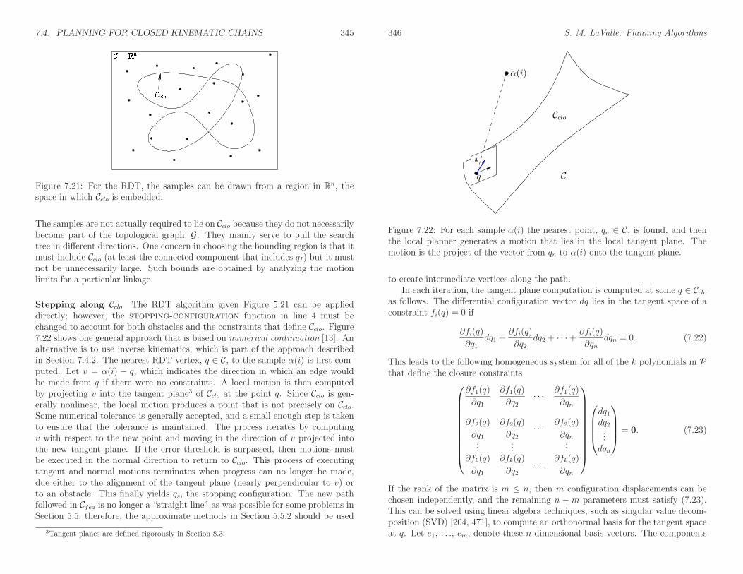
7.4. PLANNING FOR CLOSED KINEMATIC CHAINS 345C = RnC lo
Figure 7.21: For the RDT, the samples can be drawn from a region in Rn, thespace in which Cclo is embedded.
The samples are not actually required to lie on Cclo because they do not necessarilybecome part of the topological graph, G. They mainly serve to pull the searchtree in different directions. One concern in choosing the bounding region is that itmust include Cclo (at least the connected component that includes qI) but it mustnot be unnecessarily large. Such bounds are obtained by analyzing the motionlimits for a particular linkage.
Stepping along Cclo The RDT algorithm given Figure 5.21 can be applieddirectly; however, the stopping-configuration function in line 4 must bechanged to account for both obstacles and the constraints that define Cclo. Figure7.22 shows one general approach that is based on numerical continuation [13]. Analternative is to use inverse kinematics, which is part of the approach describedin Section 7.4.2. The nearest RDT vertex, q ∈ C, to the sample α(i) is first com-puted. Let v = α(i) − q, which indicates the direction in which an edge wouldbe made from q if there were no constraints. A local motion is then computedby projecting v into the tangent plane3 of Cclo at the point q. Since Cclo is gen-erally nonlinear, the local motion produces a point that is not precisely on Cclo.Some numerical tolerance is generally accepted, and a small enough step is takento ensure that the tolerance is maintained. The process iterates by computingv with respect to the new point and moving in the direction of v projected intothe new tangent plane. If the error threshold is surpassed, then motions mustbe executed in the normal direction to return to Cclo. This process of executingtangent and normal motions terminates when progress can no longer be made,due either to the alignment of the tangent plane (nearly perpendicular to v) orto an obstacle. This finally yields qs, the stopping configuration. The new pathfollowed in Cfea is no longer a “straight line” as was possible for some problems inSection 5.5; therefore, the approximate methods in Section 5.5.2 should be used
3Tangent planes are defined rigorously in Section 8.3.
346 S. M. LaValle: Planning Algorithms
α(i)
Cclo
Cq
Figure 7.22: For each sample α(i) the nearest point, qn ∈ C, is found, and thenthe local planner generates a motion that lies in the local tangent plane. Themotion is the project of the vector from qn to α(i) onto the tangent plane.
to create intermediate vertices along the path.In each iteration, the tangent plane computation is computed at some q ∈ Cclo
as follows. The differential configuration vector dq lies in the tangent space of aconstraint fi(q) = 0 if
∂fi(q)
∂q1dq1 +
∂fi(q)
∂q2dq2 + · · ·+
∂fi(q)
∂qndqn = 0. (7.22)
This leads to the following homogeneous system for all of the k polynomials in Pthat define the closure constraints
∂f1(q)
∂q1
∂f1(q)
∂q2· · · ∂f1(q)
∂qn
∂f2(q)
∂q1
∂f2(q)
∂q2· · · ∂f2(q)
∂qn...
......
∂fk(q)
∂q1
∂fk(q)
∂q2· · · ∂fk(q)
∂qn
dq1dq2...dqn
= 0. (7.23)
If the rank of the matrix is m ≤ n, then m configuration displacements can bechosen independently, and the remaining n −m parameters must satisfy (7.23).This can be solved using linear algebra techniques, such as singular value decom-position (SVD) [204, 471], to compute an orthonormal basis for the tangent spaceat q. Let e1, . . ., em, denote these n-dimensional basis vectors. The components
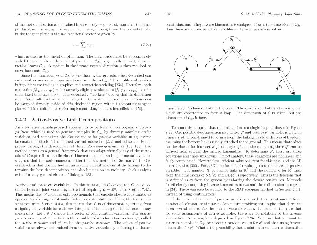
7.4. PLANNING FOR CLOSED KINEMATIC CHAINS 347
of the motion direction are obtained from v = α(i)−qn. First, construct the innerproducts, a1 = v · e1, a2 = v · e2, . . ., am = v · em. Using these, the projection of vin the tangent plane is the n-dimensional vector w given by
w =m∑
i
aiei, (7.24)
which is used as the direction of motion. The magnitude must be appropriatelyscaled to take sufficiently small steps. Since Cclo is generally curved, a linearmotion leaves Cclo. A motion in the inward normal direction is then required tomove back onto Cclo.
Since the dimension m of Cclo is less than n, the procedure just described canonly produce numerical approximations to paths in Cclo. This problem also arisesin implicit curve tracing in graphics and geometric modeling [234]. Therefore, eachconstraint fi(q1, . . . , qn) = 0 is actually slightly weakened to |fi(q1, . . . , qn)| < ǫ forsome fixed tolerance ǫ > 0. This essentially “thickens” Cclo so that its dimensionis n. As an alternative to computing the tangent plane, motion directions canbe sampled directly inside of this thickened region without computing tangentplanes. This results in an easier implementation, but it is less efficient [479].
7.4.2 Active-Passive Link Decompositions
An alternative sampling-based approach is to perform an active-passive decom-position, which is used to generate samples in Cclo by directly sampling activevariables, and computing the closure values for passive variables using inversekinematics methods. This method was introduced in [222] and subsequently im-proved through the development of the random loop generator in [133, 135]. Themethod serves as a general framework that can adapt virtually any of the meth-ods of Chapter 5 to handle closed kinematic chains, and experimental evidencesuggests that the performance is better than the method of Section 7.4.1. Onedrawback is that the method requires some careful analysis of the linkage to de-termine the best decomposition and also bounds on its mobility. Such analysisexists for very general classes of linkages [133].
Active and passive variables In this section, let C denote the C-space ob-tained from all joint variables, instead of requiring C = Rn, as in Section 7.4.1.This means that P includes only polynomials that encode closure constraints, asopposed to allowing constraints that represent rotations. Using the tree repre-sentation from Section 4.4.3, this means that C is of dimension n, arising fromassigning one variable for each revolute joint of the linkage in the absence of anyconstraints. Let q ∈ C denote this vector of configuration variables. The active-passive decomposition partitions the variables of q to form two vectors, qa, calledthe active variables and qp, called the passive variables. The values of passivevariables are always determined from the active variables by enforcing the closure
348 S. M. LaValle: Planning Algorithms
constraints and using inverse kinematics techniques. If m is the dimension of Cclo,then there are always m active variables and n−m passive variables.
θ2
θ4
θ5 θ6
θ1 θ7
θ3
Figure 7.23: A chain of links in the plane. There are seven links and seven joints,which are constrained to form a loop. The dimension of C is seven, but thedimension of Cclo is four.
Temporarily, suppose that the linkage forms a single loop as shown in Figure7.23. One possible decomposition into active qa and passive qp variables is given inFigure 7.24. If constrained to form a loop, the linkage has four degrees of freedom,assuming the bottom link is rigidly attached to the ground. This means that valuescan be chosen for four active joint angles qa and the remaining three qp can bederived from solving the inverse kinematics. To determine qp, there are threeequations and three unknowns. Unfortunately, these equations are nonlinear andfairly complicated. Nevertheless, efficient solutions exist for this case, and the 3Dgeneralization [350]. For a 3D loop formed of revolute joints, there are six passivevariables. The number, 3, of passive links in R2 and the number 6 for R3 arisefrom the dimensions of SE(2) and SE(3), respectively. This is the freedom thatis stripped away from the system by enforcing the closure constraints. Methodsfor efficiently computing inverse kinematics in two and three dimensions are givenin [24]. These can also be applied to the RDT stepping method in Section 7.4.1,instead of using continuation.
If the maximal number of passive variables is used, there is at most a finitenumber of solutions to the inverse kinematics problem; this implies that there areoften several choices for the passive variable values. It could be the case thatfor some assignments of active variables, there are no solutions to the inversekinematics. An example is depicted in Figure 7.25. Suppose that we want togenerate samples in Cclo by selecting random values for qa and then using inversekinematics for qp. What is the probability that a solution to the inverse kinematics
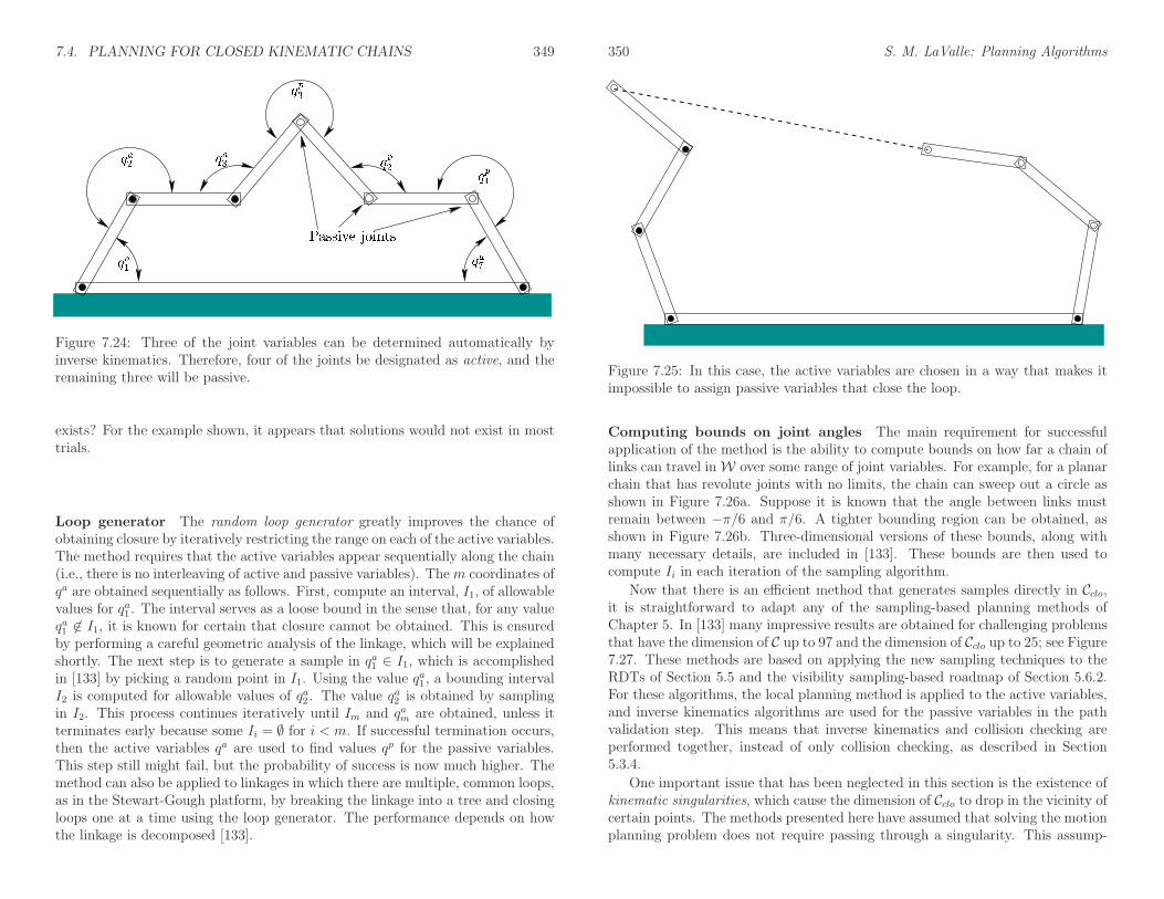
7.4. PLANNING FOR CLOSED KINEMATIC CHAINS 349
qp2
qa1qa2 qa3
qa7qp3
Passive joints qp1
Figure 7.24: Three of the joint variables can be determined automatically byinverse kinematics. Therefore, four of the joints be designated as active, and theremaining three will be passive.
exists? For the example shown, it appears that solutions would not exist in mosttrials.
Loop generator The random loop generator greatly improves the chance ofobtaining closure by iteratively restricting the range on each of the active variables.The method requires that the active variables appear sequentially along the chain(i.e., there is no interleaving of active and passive variables). Them coordinates ofqa are obtained sequentially as follows. First, compute an interval, I1, of allowablevalues for qa1 . The interval serves as a loose bound in the sense that, for any valueqa1 6∈ I1, it is known for certain that closure cannot be obtained. This is ensuredby performing a careful geometric analysis of the linkage, which will be explainedshortly. The next step is to generate a sample in qa1 ∈ I1, which is accomplishedin [133] by picking a random point in I1. Using the value qa1 , a bounding intervalI2 is computed for allowable values of qa2 . The value qa2 is obtained by samplingin I2. This process continues iteratively until Im and qam are obtained, unless itterminates early because some Ii = ∅ for i < m. If successful termination occurs,then the active variables qa are used to find values qp for the passive variables.This step still might fail, but the probability of success is now much higher. Themethod can also be applied to linkages in which there are multiple, common loops,as in the Stewart-Gough platform, by breaking the linkage into a tree and closingloops one at a time using the loop generator. The performance depends on howthe linkage is decomposed [133].
350 S. M. LaValle: Planning Algorithms
Figure 7.25: In this case, the active variables are chosen in a way that makes itimpossible to assign passive variables that close the loop.
Computing bounds on joint angles The main requirement for successfulapplication of the method is the ability to compute bounds on how far a chain oflinks can travel inW over some range of joint variables. For example, for a planarchain that has revolute joints with no limits, the chain can sweep out a circle asshown in Figure 7.26a. Suppose it is known that the angle between links mustremain between −π/6 and π/6. A tighter bounding region can be obtained, asshown in Figure 7.26b. Three-dimensional versions of these bounds, along withmany necessary details, are included in [133]. These bounds are then used tocompute Ii in each iteration of the sampling algorithm.
Now that there is an efficient method that generates samples directly in Cclo,it is straightforward to adapt any of the sampling-based planning methods ofChapter 5. In [133] many impressive results are obtained for challenging problemsthat have the dimension of C up to 97 and the dimension of Cclo up to 25; see Figure7.27. These methods are based on applying the new sampling techniques to theRDTs of Section 5.5 and the visibility sampling-based roadmap of Section 5.6.2.For these algorithms, the local planning method is applied to the active variables,and inverse kinematics algorithms are used for the passive variables in the pathvalidation step. This means that inverse kinematics and collision checking areperformed together, instead of only collision checking, as described in Section5.3.4.
One important issue that has been neglected in this section is the existence ofkinematic singularities, which cause the dimension of Cclo to drop in the vicinity ofcertain points. The methods presented here have assumed that solving the motionplanning problem does not require passing through a singularity. This assump-
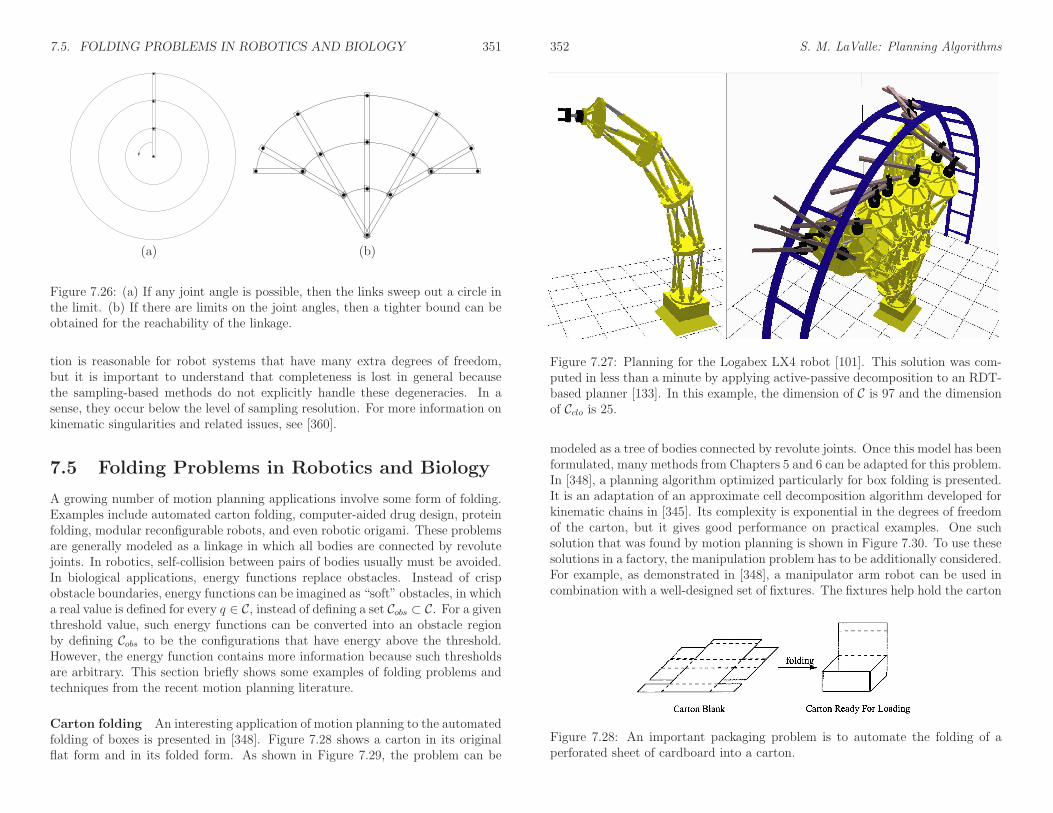
7.5. FOLDING PROBLEMS IN ROBOTICS AND BIOLOGY 351
(a) (b)
Figure 7.26: (a) If any joint angle is possible, then the links sweep out a circle inthe limit. (b) If there are limits on the joint angles, then a tighter bound can beobtained for the reachability of the linkage.
tion is reasonable for robot systems that have many extra degrees of freedom,but it is important to understand that completeness is lost in general becausethe sampling-based methods do not explicitly handle these degeneracies. In asense, they occur below the level of sampling resolution. For more information onkinematic singularities and related issues, see [360].
7.5 Folding Problems in Robotics and Biology
A growing number of motion planning applications involve some form of folding.Examples include automated carton folding, computer-aided drug design, proteinfolding, modular reconfigurable robots, and even robotic origami. These problemsare generally modeled as a linkage in which all bodies are connected by revolutejoints. In robotics, self-collision between pairs of bodies usually must be avoided.In biological applications, energy functions replace obstacles. Instead of crispobstacle boundaries, energy functions can be imagined as “soft” obstacles, in whicha real value is defined for every q ∈ C, instead of defining a set Cobs ⊂ C. For a giventhreshold value, such energy functions can be converted into an obstacle regionby defining Cobs to be the configurations that have energy above the threshold.However, the energy function contains more information because such thresholdsare arbitrary. This section briefly shows some examples of folding problems andtechniques from the recent motion planning literature.
Carton folding An interesting application of motion planning to the automatedfolding of boxes is presented in [348]. Figure 7.28 shows a carton in its originalflat form and in its folded form. As shown in Figure 7.29, the problem can be
352 S. M. LaValle: Planning Algorithms
Figure 7.27: Planning for the Logabex LX4 robot [101]. This solution was com-puted in less than a minute by applying active-passive decomposition to an RDT-based planner [133]. In this example, the dimension of C is 97 and the dimensionof Cclo is 25.
modeled as a tree of bodies connected by revolute joints. Once this model has beenformulated, many methods from Chapters 5 and 6 can be adapted for this problem.In [348], a planning algorithm optimized particularly for box folding is presented.It is an adaptation of an approximate cell decomposition algorithm developed forkinematic chains in [345]. Its complexity is exponential in the degrees of freedomof the carton, but it gives good performance on practical examples. One suchsolution that was found by motion planning is shown in Figure 7.30. To use thesesolutions in a factory, the manipulation problem has to be additionally considered.For example, as demonstrated in [348], a manipulator arm robot can be used incombination with a well-designed set of fixtures. The fixtures help hold the carton
Figure 7.28: An important packaging problem is to automate the folding of aperforated sheet of cardboard into a carton.

7.5. FOLDING PROBLEMS IN ROBOTICS AND BIOLOGY 353
Figure 7.29: The carton can be cleverly modeled as a tree of bodies that areattached by revolute joints.
Figure 7.30: A folding sequence that was computed using the algorithm in [348].
354 S. M. LaValle: Planning Algorithms
in place while the manipulator applies pressure in the right places, which yieldsthe required folds. Since the feasibility with fixtures depends on the particularfolding path, the planning algorithm generates all possible distinct paths from theinitial configuration (at which the box is completely unfolded).
Simplifying knots A knot is a closed curve that does not intersect itself, isembedded in R3, and cannot be untangled to produce a simple loop (such as acircular path). If the knot is allowed to intersect itself, then any knot can beuntangled; therefore, a careful definition of what it means to untangle a knot isneeded. For a closed curve, τ : [0, 1] → R3, embedded in R3 (it cannot intersectitself), let the set R3 \ τ([0, 1]) of points not reached by the curve be called theambient space of τ . In knot theory, an ambient isotopy between two closed curves,τ1 and τ2, embedded in R3 is a homeomorphism between their ambient spaces.Intuitively, this means that τ1 can be warped into τ2 without allowing any self-intersections. Therefore, determining whether two loops are equivalent seemsclosely related to motion planning. Such equivalence gives rise to groups thatcharacterize the space of knots and are closely related to the fundamental groupdescribed in Section 4.1.3. For more information on knot theory, see [6, 232, 261].
A motion planning approach was developed in [297] to determine whether aclosed curve is equivalent to the unknot, which is completely untangled. Thiscan be expressed as a curve that maps onto S1, embedded in R3. The algorithmtakes as input a knot expressed as a circular chain of line segments embedded inR3. In this case, the unknot can be expressed as a triangle in R3. One of themost challenging examples solved by the planner is shown in Figure 7.31. Theplanner is sampling-based and shares many similarities with the RDT algorithmof Section 5.5 and the Ariadne’s clew and expansive space planners described inSection 5.4.4. Since the task is not to produce a collision-free path, there areseveral unique aspects in comparison to motion planning. An energy function isdefined over the collection of segments to try to guide the search toward simplerconfigurations. There are two kinds of local operations that are made by theplanner: 1) Try to move a vertex toward a selected subgoal in the ambient space.This is obtained by using random sampling to grow a search tree. 2) Try to deletea vertex, and connect the neighboring vertices by a straight line. If no collisionoccurs along the intermediate configurations, then the knot has been simplified.The algorithm terminates when it is unable to further simplify the knot.
Drug design A sampling-based motion planning approach to pharmaceuticaldrug design is taken in [308]. The development of a drug is a long, incrementalprocess, typically requiring years of research and experimentation. The goal isto find a relatively small molecule called a ligand, typically comprising a fewdozen atoms, that docks with a receptor cavity in a specific protein [315]; Figure1.14 (Section 1.2) illustrated this. Examples of drug molecules were also givenin Figure 1.14. Protein-ligand docking can stimulate or inhibit some biological
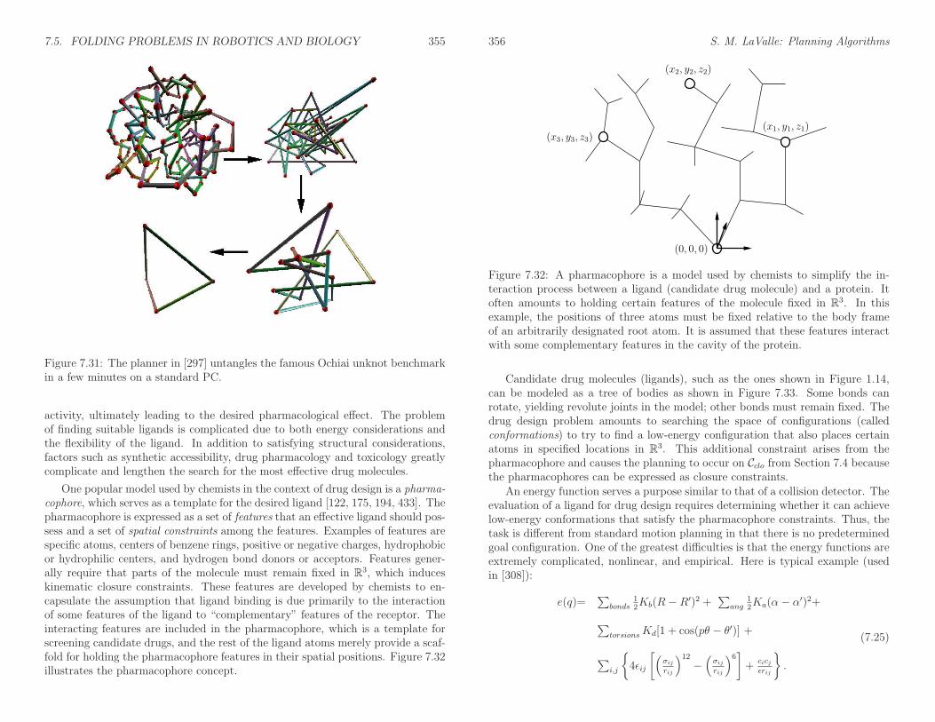
7.5. FOLDING PROBLEMS IN ROBOTICS AND BIOLOGY 355
Figure 7.31: The planner in [297] untangles the famous Ochiai unknot benchmarkin a few minutes on a standard PC.
activity, ultimately leading to the desired pharmacological effect. The problemof finding suitable ligands is complicated due to both energy considerations andthe flexibility of the ligand. In addition to satisfying structural considerations,factors such as synthetic accessibility, drug pharmacology and toxicology greatlycomplicate and lengthen the search for the most effective drug molecules.
One popular model used by chemists in the context of drug design is a pharma-cophore, which serves as a template for the desired ligand [122, 175, 194, 433]. Thepharmacophore is expressed as a set of features that an effective ligand should pos-sess and a set of spatial constraints among the features. Examples of features arespecific atoms, centers of benzene rings, positive or negative charges, hydrophobicor hydrophilic centers, and hydrogen bond donors or acceptors. Features gener-ally require that parts of the molecule must remain fixed in R3, which induceskinematic closure constraints. These features are developed by chemists to en-capsulate the assumption that ligand binding is due primarily to the interactionof some features of the ligand to “complementary” features of the receptor. Theinteracting features are included in the pharmacophore, which is a template forscreening candidate drugs, and the rest of the ligand atoms merely provide a scaf-fold for holding the pharmacophore features in their spatial positions. Figure 7.32illustrates the pharmacophore concept.
356 S. M. LaValle: Planning Algorithms
(x2, y2, z2)
(x1, y1, z1)(x3, y3, z3)
(0, 0, 0)
Figure 7.32: A pharmacophore is a model used by chemists to simplify the in-teraction process between a ligand (candidate drug molecule) and a protein. Itoften amounts to holding certain features of the molecule fixed in R3. In thisexample, the positions of three atoms must be fixed relative to the body frameof an arbitrarily designated root atom. It is assumed that these features interactwith some complementary features in the cavity of the protein.
Candidate drug molecules (ligands), such as the ones shown in Figure 1.14,can be modeled as a tree of bodies as shown in Figure 7.33. Some bonds canrotate, yielding revolute joints in the model; other bonds must remain fixed. Thedrug design problem amounts to searching the space of configurations (calledconformations) to try to find a low-energy configuration that also places certainatoms in specified locations in R3. This additional constraint arises from thepharmacophore and causes the planning to occur on Cclo from Section 7.4 becausethe pharmacophores can be expressed as closure constraints.
An energy function serves a purpose similar to that of a collision detector. Theevaluation of a ligand for drug design requires determining whether it can achievelow-energy conformations that satisfy the pharmacophore constraints. Thus, thetask is different from standard motion planning in that there is no predeterminedgoal configuration. One of the greatest difficulties is that the energy functions areextremely complicated, nonlinear, and empirical. Here is typical example (usedin [308]):
e(q)=∑
bonds12Kb(R− R′)2 +
∑
ang12Ka(α− α′)2+
∑
torsionsKd[1 + cos(pθ − θ′)] +
∑
i,j
4ǫij
[
(
σij
rij
)12
−(
σij
rij
)6]
+cicjǫrij
.
(7.25)
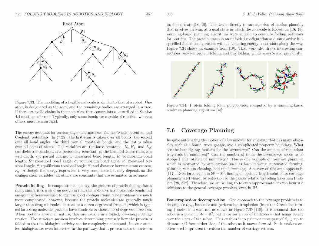
7.5. FOLDING PROBLEMS IN ROBOTICS AND BIOLOGY 357
θ1 θ2
θ3
θ5
θ6
θ4
Root Atom
Figure 7.33: The modeling of a flexible molecule is similar to that of a robot. Oneatom is designated as the root, and the remaining bodies are arranged in a tree.If there are cyclic chains in the molecules, then constraints as described in Section4.4 must be enforced. Typically, only some bonds are capable of rotation, whereasothers must remain rigid.
The energy accounts for torsion-angle deformations, van der Waals potential, andCoulomb potentials. In (7.25), the first sum is taken over all bonds, the secondover all bond angles, the third over all rotatable bonds, and the last is takenover all pairs of atoms. The variables are the force constants, Kb, Ka, and Kd;the dielectric constant, ǫ; a periodicity constant, p; the Lennard-Jones radii, σij ;well depth, ǫij; partial charge, ci; measured bond length, R; equilibrium bondlength, R′; measured bond angle, α; equilibrium bond angle, α′; measured tor-sional angle, θ; equilibrium torsional angle, θ′; and distance between atom centers,rij. Although the energy expression is very complicated, it only depends on theconfiguration variables; all others are constants that are estimated in advance.
Protein folding In computational biology, the problem of protein folding sharesmany similarities with drug design in that the molecules have rotatable bonds andenergy functions are used to express good configurations. The problems are muchmore complicated, however, because the protein molecules are generally muchlarger than drug molecules. Instead of a dozen degrees of freedom, which is typi-cal for a drug molecule, proteins have hundreds or thousands of degrees of freedom.When proteins appear in nature, they are usually in a folded, low-energy config-uration. The structure problem involves determining precisely how the protein isfolded so that its biological activity can be completely understood. In some stud-ies, biologists are even interested in the pathway that a protein takes to arrive in
358 S. M. LaValle: Planning Algorithms
its folded state [18, 19]. This leads directly to an extension of motion planningthat involves arriving at a goal state in which the molecule is folded. In [18, 19],sampling-based planning algorithms were applied to compute folding pathwaysfor proteins. The protein starts in an unfolded configuration and must arrive in aspecified folded configuration without violating energy constraints along the way.Figure 7.34 shows an example from [19]. That work also draws interesting con-nections between protein folding and box folding, which was covered previously.
Figure 7.34: Protein folding for a polypeptide, computed by a sampling-basedroadmap planning algorithm [18]
7.6 Coverage Planning
Imagine automating the motion of a lawnmower for an estate that has many obsta-cles, such as a house, trees, garage, and a complicated property boundary. Whatare the best zig-zag motions for the lawnmower? Can the amount of redundanttraversals be minimized? Can the number of times the lawnmower needs to bestopped and rotated be minimized? This is one example of coverage planning,which is motivated by applications such as lawn mowing, automated farming,painting, vacuum cleaning, and mine sweeping. A survey of this area appears in[117]. Even for a region inW = R2, finding an optimal-length solution to coverageplanning is NP-hard, by reduction to the closely related Traveling Salesman Prob-lem [28, 372]. Therefore, we are willing to tolerate approximate or even heuristicsolutions to the general coverage problem, even in R2.
Boustrophedon decomposition One approach to the coverage problem is todecompose Cfree into cells and perform boustrophedon (from the Greek “ox turn-ing”) motions in each cell as shown in Figure 7.35 [119]. It is assumed that therobot is a point in W = R2, but it carries a tool of thickness ǫ that hangs evenlyover the sides of the robot. This enables it to paint or mow part of Cfree up todistance ǫ/2 from either side of the robot as it moves forward. Such motions areoften used in printers to reduce the number of carriage returns.

7.6. COVERAGE PLANNING 359
Figure 7.35: An example of the ox plowing motions.
(a) (b)
Figure 7.36: (a) Only the first case from Figure 6.2 is needed: extend upwardand downward. All other cases are neglected. (b) The resulting decompositionis shown, which has fewer cells than that of the vertical decomposition in Figure6.3.
If Cobs is polygonal, a reasonable decomposition can be obtained by adaptingthe vertical decomposition method of Section 6.2.2. In that algorithm, criticalevents were defined for several cases, some of which are not relevant for the bous-trophedon motions. The only events that need to be handled are shown in Figure7.36a [116]. This produces a decomposition that has fewer cells, as shown in Fig-ure 7.36b. Even though the cells are nonconvex, they can always be sliced nicelyinto vertical strips, which makes them suitable for boustrophedon motions. Theoriginal vertical decomposition could also be used, but the extra cell boundarieswould cause unnecessary repositioning of the robot. A similar method, whichfurthermore optimizes the number of robot turns, is presented in [243].
Spanning tree covering An interesting approximate method was developedby Gabriely and Rimon; it places a tiling of squares inside of Cfree and computesthe spanning tree of the resulting connectivity graph [187, 188]. Suppose againthat Cfree is polygonal. Consider the example shown in Figure 7.37a. The first
360 S. M. LaValle: Planning Algorithms
(a) (b)
(c) (d)
Figure 7.37: (a) An example used for spanning tree covering. (b) The first step isto tile the interior with squares. (c) The spanning tree of a roadmap formed fromgrid adjacencies. (d) The resulting coverage path.
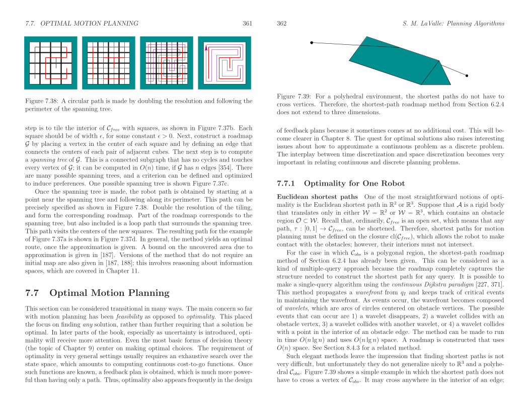
7.7. OPTIMAL MOTION PLANNING 361
Figure 7.38: A circular path is made by doubling the resolution and following theperimeter of the spanning tree.
step is to tile the interior of Cfree with squares, as shown in Figure 7.37b. Eachsquare should be of width ǫ, for some constant ǫ > 0. Next, construct a roadmapG by placing a vertex in the center of each square and by defining an edge thatconnects the centers of each pair of adjacent cubes. The next step is to computea spanning tree of G. This is a connected subgraph that has no cycles and touchesevery vertex of G; it can be computed in O(n) time, if G has n edges [354]. Thereare many possible spanning trees, and a criterion can be defined and optimizedto induce preferences. One possible spanning tree is shown Figure 7.37c.
Once the spanning tree is made, the robot path is obtained by starting at apoint near the spanning tree and following along its perimeter. This path can beprecisely specified as shown in Figure 7.38. Double the resolution of the tiling,and form the corresponding roadmap. Part of the roadmap corresponds to thespanning tree, but also included is a loop path that surrounds the spanning tree.This path visits the centers of the new squares. The resulting path for the exampleof Figure 7.37a is shown in Figure 7.37d. In general, the method yields an optimalroute, once the approximation is given. A bound on the uncovered area due toapproximation is given in [187]. Versions of the method that do not require aninitial map are also given in [187, 188]; this involves reasoning about informationspaces, which are covered in Chapter 11.
7.7 Optimal Motion Planning
This section can be considered transitional in many ways. The main concern so farwith motion planning has been feasibility as opposed to optimality. This placedthe focus on finding any solution, rather than further requiring that a solution beoptimal. In later parts of the book, especially as uncertainty is introduced, opti-mality will receive more attention. Even the most basic forms of decision theory(the topic of Chapter 9) center on making optimal choices. The requirement ofoptimality in very general settings usually requires an exhaustive search over thestate space, which amounts to computing continuous cost-to-go functions. Oncesuch functions are known, a feedback plan is obtained, which is much more power-ful than having only a path. Thus, optimality also appears frequently in the design
362 S. M. LaValle: Planning Algorithms
Figure 7.39: For a polyhedral environment, the shortest paths do not have tocross vertices. Therefore, the shortest-path roadmap method from Section 6.2.4does not extend to three dimensions.
of feedback plans because it sometimes comes at no additional cost. This will be-come clearer in Chapter 8. The quest for optimal solutions also raises interestingissues about how to approximate a continuous problem as a discrete problem.The interplay between time discretization and space discretization becomes veryimportant in relating continuous and discrete planning problems.
7.7.1 Optimality for One Robot
Euclidean shortest paths One of the most straightforward notions of opti-mality is the Euclidean shortest path in R2 or R3. Suppose that A is a rigid bodythat translates only in either W = R2 or W = R3, which contains an obstacleregion O ⊂ W . Recall that, ordinarily, Cfree is an open set, which means that anypath, τ : [0, 1] → Cfree, can be shortened. Therefore, shortest paths for motionplanning must be defined on the closure cl(Cfree), which allows the robot to makecontact with the obstacles; however, their interiors must not intersect.
For the case in which Cobs is a polygonal region, the shortest-path roadmapmethod of Section 6.2.4 has already been given. This can be considered as akind of multiple-query approach because the roadmap completely captures thestructure needed to construct the shortest path for any query. It is possible tomake a single-query algorithm using the continuous Dijkstra paradigm [227, 371].This method propagates a wavefront from qI and keeps track of critical eventsin maintaining the wavefront. As events occur, the wavefront becomes composedof wavelets, which are arcs of circles centered on obstacle vertices. The possibleevents that can occur are 1) a wavelet disappears, 2) a wavelet collides with anobstacle vertex, 3) a wavelet collides with another wavelet, or 4) a wavelet collideswith a point in the interior of an obstacle edge. The method can be made to runin time O(n lg n) and uses O(n lg n) space. A roadmap is constructed that usesO(n) space. See Section 8.4.3 for a related method.
Such elegant methods leave the impression that finding shortest paths is notvery difficult, but unfortunately they do not generalize nicely to R3 and a polyhe-dral Cobs. Figure 7.39 shows a simple example in which the shortest path does nothave to cross a vertex of Cobs. It may cross anywhere in the interior of an edge;
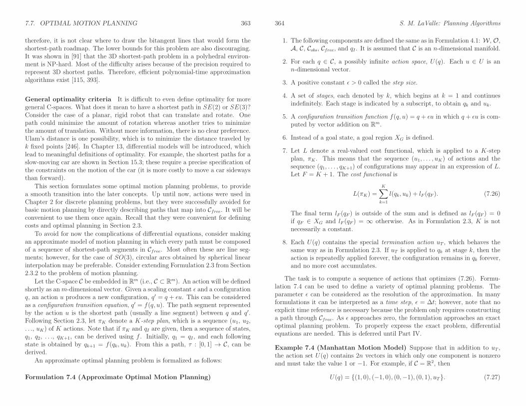
7.7. OPTIMAL MOTION PLANNING 363
therefore, it is not clear where to draw the bitangent lines that would form theshortest-path roadmap. The lower bounds for this problem are also discouraging.It was shown in [91] that the 3D shortest-path problem in a polyhedral environ-ment is NP-hard. Most of the difficulty arises because of the precision required torepresent 3D shortest paths. Therefore, efficient polynomial-time approximationalgorithms exist [115, 393].
General optimality criteria It is difficult to even define optimality for moregeneral C-spaces. What does it mean to have a shortest path in SE(2) or SE(3)?Consider the case of a planar, rigid robot that can translate and rotate. Onepath could minimize the amount of rotation whereas another tries to minimizethe amount of translation. Without more information, there is no clear preference.Ulam’s distance is one possibility, which is to minimize the distance traveled byk fixed points [246]. In Chapter 13, differential models will be introduced, whichlead to meaningful definitions of optimality. For example, the shortest paths for aslow-moving car are shown in Section 15.3; these require a precise specification ofthe constraints on the motion of the car (it is more costly to move a car sidewaysthan forward).
This section formulates some optimal motion planning problems, to providea smooth transition into the later concepts. Up until now, actions were used inChapter 2 for discrete planning problems, but they were successfully avoided forbasic motion planning by directly describing paths that map into Cfree. It will beconvenient to use them once again. Recall that they were convenient for definingcosts and optimal planning in Section 2.3.
To avoid for now the complications of differential equations, consider makingan approximate model of motion planning in which every path must be composedof a sequence of shortest-path segments in Cfree. Most often these are line seg-ments; however, for the case of SO(3), circular arcs obtained by spherical linearinterpolation may be preferable. Consider extending Formulation 2.3 from Section2.3.2 to the problem of motion planning.
Let the C-space C be embedded in Rm (i.e., C ⊂ Rm). An action will be definedshortly as anm-dimensional vector. Given a scaling constant ǫ and a configurationq, an action u produces a new configuration, q′ = q + ǫu. This can be consideredas a configuration transition equation, q′ = f(q, u). The path segment representedby the action u is the shortest path (usually a line segment) between q and q′.Following Section 2.3, let πK denote a K-step plan, which is a sequence (u1, u2,. . ., uK) of K actions. Note that if πK and qI are given, then a sequence of states,q1, q2, . . ., qK+1, can be derived using f . Initially, q1 = qI , and each followingstate is obtained by qk+1 = f(qk, uk). From this a path, τ : [0, 1] → C, can bederived.
An approximate optimal planning problem is formalized as follows:
Formulation 7.4 (Approximate Optimal Motion Planning)
364 S. M. LaValle: Planning Algorithms
1. The following components are defined the same as in Formulation 4.1: W , O,A, C, Cobs, Cfree, and qI . It is assumed that C is an n-dimensional manifold.
2. For each q ∈ C, a possibly infinite action space, U(q). Each u ∈ U is ann-dimensional vector.
3. A positive constant ǫ > 0 called the step size.
4. A set of stages, each denoted by k, which begins at k = 1 and continuesindefinitely. Each stage is indicated by a subscript, to obtain qk and uk.
5. A configuration transition function f(q, u) = q + ǫu in which q + ǫu is com-puted by vector addition on Rm.
6. Instead of a goal state, a goal region XG is defined.
7. Let L denote a real-valued cost functional, which is applied to a K-stepplan, πK . This means that the sequence (u1, . . . , uK) of actions and thesequence (q1, . . . , qK+1) of configurations may appear in an expression of L.Let F = K + 1. The cost functional is
L(πK) =K∑
k=1
l(qk, uk) + lF (qF ). (7.26)
The final term lF (qF ) is outside of the sum and is defined as lF (qF ) = 0if qF ∈ XG and lF (qF ) = ∞ otherwise. As in Formulation 2.3, K is notnecessarily a constant.
8. Each U(q) contains the special termination action uT , which behaves thesame way as in Formulation 2.3. If uT is applied to qk at stage k, then theaction is repeatedly applied forever, the configuration remains in qk forever,and no more cost accumulates.
The task is to compute a sequence of actions that optimizes (7.26). Formu-lation 7.4 can be used to define a variety of optimal planning problems. Theparameter ǫ can be considered as the resolution of the approximation. In manyformulations it can be interpreted as a time step, ǫ = ∆t; however, note that noexplicit time reference is necessary because the problem only requires constructinga path through Cfree. As ǫ approaches zero, the formulation approaches an exactoptimal planning problem. To properly express the exact problem, differentialequations are needed. This is deferred until Part IV.
Example 7.4 (Manhattan Motion Model) Suppose that in addition to uT ,the action set U(q) contains 2n vectors in which only one component is nonzeroand must take the value 1 or −1. For example, if C = R2, then
U(q) = (1, 0), (−1, 0), (0,−1), (0, 1), uT. (7.27)
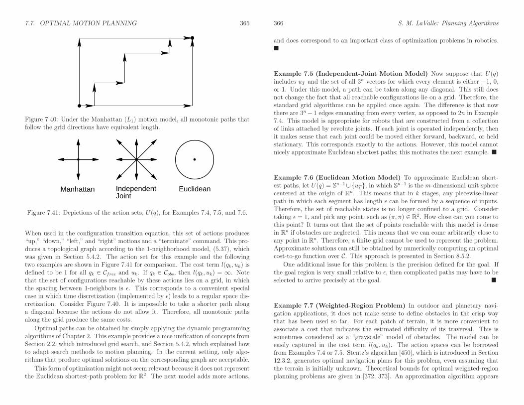
7.7. OPTIMAL MOTION PLANNING 365
Figure 7.40: Under the Manhattan (L1) motion model, all monotonic paths thatfollow the grid directions have equivalent length.
IndependentJoint
EuclideanManhattan
Figure 7.41: Depictions of the action sets, U(q), for Examples 7.4, 7.5, and 7.6.
When used in the configuration transition equation, this set of actions produces“up,” “down,” “left,” and “right” motions and a “terminate” command. This pro-duces a topological graph according to the 1-neighborhood model, (5.37), whichwas given in Section 5.4.2. The action set for this example and the followingtwo examples are shown in Figure 7.41 for comparison. The cost term l(qk, uk) isdefined to be 1 for all qk ∈ Cfree and uk. If qk ∈ Cobs, then l(qk, uk) = ∞. Notethat the set of configurations reachable by these actions lies on a grid, in whichthe spacing between 1-neighbors is ǫ. This corresponds to a convenient specialcase in which time discretization (implemented by ǫ) leads to a regular space dis-cretization. Consider Figure 7.40. It is impossible to take a shorter path alonga diagonal because the actions do not allow it. Therefore, all monotonic pathsalong the grid produce the same costs.
Optimal paths can be obtained by simply applying the dynamic programmingalgorithms of Chapter 2. This example provides a nice unification of concepts fromSection 2.2, which introduced grid search, and Section 5.4.2, which explained howto adapt search methods to motion planning. In the current setting, only algo-rithms that produce optimal solutions on the corresponding graph are acceptable.
This form of optimization might not seem relevant because it does not representthe Euclidean shortest-path problem for R2. The next model adds more actions,
366 S. M. LaValle: Planning Algorithms
and does correspond to an important class of optimization problems in robotics.
Example 7.5 (Independent-Joint Motion Model) Now suppose that U(q)includes uT and the set of all 3n vectors for which every element is either −1, 0,or 1. Under this model, a path can be taken along any diagonal. This still doesnot change the fact that all reachable configurations lie on a grid. Therefore, thestandard grid algorithms can be applied once again. The difference is that nowthere are 3n− 1 edges emanating from every vertex, as opposed to 2n in Example7.4. This model is appropriate for robots that are constructed from a collectionof links attached by revolute joints. If each joint is operated independently, thenit makes sense that each joint could be moved either forward, backward, or heldstationary. This corresponds exactly to the actions. However, this model cannotnicely approximate Euclidean shortest paths; this motivates the next example.
Example 7.6 (Euclidean Motion Model) To approximate Euclidean short-est paths, let U(q) = Sn−1∪uT, in which Sn−1 is the m-dimensional unit spherecentered at the origin of Rn. This means that in k stages, any piecewise-linearpath in which each segment has length ǫ can be formed by a sequence of inputs.Therefore, the set of reachable states is no longer confined to a grid. Considertaking ǫ = 1, and pick any point, such as (π, π) ∈ R2. How close can you come tothis point? It turns out that the set of points reachable with this model is densein Rn if obstacles are neglected. This means that we can come arbitrarily close toany point in Rn. Therefore, a finite grid cannot be used to represent the problem.Approximate solutions can still be obtained by numerically computing an optimalcost-to-go function over C. This approach is presented in Section 8.5.2.
One additional issue for this problem is the precision defined for the goal. Ifthe goal region is very small relative to ǫ, then complicated paths may have to beselected to arrive precisely at the goal.
Example 7.7 (Weighted-Region Problem) In outdoor and planetary navi-gation applications, it does not make sense to define obstacles in the crisp waythat has been used so far. For each patch of terrain, it is more convenient toassociate a cost that indicates the estimated difficulty of its traversal. This issometimes considered as a “grayscale” model of obstacles. The model can beeasily captured in the cost term l(qk, uk). The action spaces can be borrowedfrom Examples 7.4 or 7.5. Stentz’s algorithm [450], which is introduced in Section12.3.2, generates optimal navigation plans for this problem, even assuming thatthe terrain is initially unknown. Theoretical bounds for optimal weighted-regionplanning problems are given in [372, 373]. An approximation algorithm appears

7.7. OPTIMAL MOTION PLANNING 367
A2A1
Figure 7.42: There are two Pareto-optimal coordination plans for this problem,depending on which robot has to wait.
in [412].
7.7.2 Multiple-Robot Optimality
Suppose that there are two robots as shown in Figure 7.42. There is just enoughroom to enable the robots to translate along the corridors. Each would like toarrive at the bottom, as indicated by arrows; however, only one can pass at atime through the horizontal corridor. Suppose that at any instant each robot caneither be on or off. When it is on, it moves at its maximum speed, and when itis off, it is stopped.4 Now suppose that each robot would like to reach its goal asquickly as possible. This means each would like to minimize the total amount oftime that it is off. In this example, there appears to be only two sensible choices:1) A1 stays on and moves straight to its goal while A2 is off just long enoughto let A1 pass, and then moves to its goal. 2) The opposite situation occurs, inwhich A2 stays on and A1 must wait. Note that when a robot waits, there aremultiple locations at which it can wait and still yield the same time to reach thegoal. The only important information is how long the robot was off.
Thus, the two interesting plans are that either A2 is off for some amount oftime, toff > 0, or A1 is off for time toff . Consider a vector of costs of the form(L1, L2), in which each component represents the cost for each robot. The costsof the plans could be measured in terms of time wasted by waiting. This yields
4This model allows infinite acceleration. Imagine that the speeds are slow enough to allowthis approximation. If this is still not satisfactory, then jump ahead to Chapter 13.
368 S. M. LaValle: Planning Algorithms
(0, toff ) and (toff , 0) for the cost vectors associated with the two plans (we couldequivalently define cost to be the total time traveled by each robot; the timeon is the same for both robots and can be subtracted from each for this simpleexample). The two plans are better than or equivalent to any others. Plans withthis property are called Pareto optimal (or nondominated). For example, if A2
waits 1 second too long for A1 to pass, then the resulting costs are (0, toff + 1),which is clearly worse than (0, toff ). The resulting plan is not Pareto optimal.More details on Pareto optimality appear in Section 9.1.1.
Another way to solve the problem is to scalarize the costs by mapping themto a single value. For example, we could find plans that optimize the averagewasted time. In this case, one of the two best plans would be obtained, yield-ing toff average wasted time. However, no information is retained about whichrobot had to make the sacrifice. Scalarizing the costs usually imposes some kindof artificial preference or prioritization among the robots. Ultimately, only oneplan can be chosen, which might make it seem inappropriate to maintain multiplesolutions. However, finding and presenting the alternative Pareto-optimal solu-tions could provide valuable information if, for example, these robots are involvedin a complicated application that involves many other time-dependent processes.Presenting the Pareto-optimal solutions is equivalent to discarding all of the worseplans and showing the best alternatives. In some applications, priorities betweenrobots may change, and if a scheduler of robots has access to the Pareto-optimalsolutions, it is easy to change priorities by switching between Pareto-optimal planswithout having to generate new plans each time.
Now the Pareto-optimality concept will be made more precise and general.Suppose there are m robots, A1, . . ., Am. Let γ refer to a motion plan thatgives the paths and timing functions for all robots. For each Ai, let Li denoteits cost functional, which yields a value Li(γ) ∈ [0,∞] for a given plan, γ. Anm-dimensional vector, L(γ), is defined as
L(γ) = (L1(γ), L2(γ), . . . , Lm(γ)). (7.28)
Two plans, γ and γ′, are called equivalent if L(γ) = L(γ′). A plan γ is saidto dominate a plan γ′ if they are not equivalent and Li(γ) ≤ Li(γ
′) for all isuch that 1 ≤ i ≤ m. A plan is called Pareto optimal if it is not dominatedby any others. Since many Pareto-optimal plans may be equivalent, the task isto determine one representative from each equivalence class. This will be calledfinding the unique Pareto-optimal plans. For the example in Figure 7.42, thereare two unique Pareto-optimal plans, which were already given.
Scalarization For the motion planning problem, a Pareto-optimal solution isalso optimal for a scalar cost functional that is constructed as a linear combinationof the individual costs. Let α1, . . ., αm be positive real constants, and let
l(γ) =m∑
i=1
αiLi(γ). (7.29)
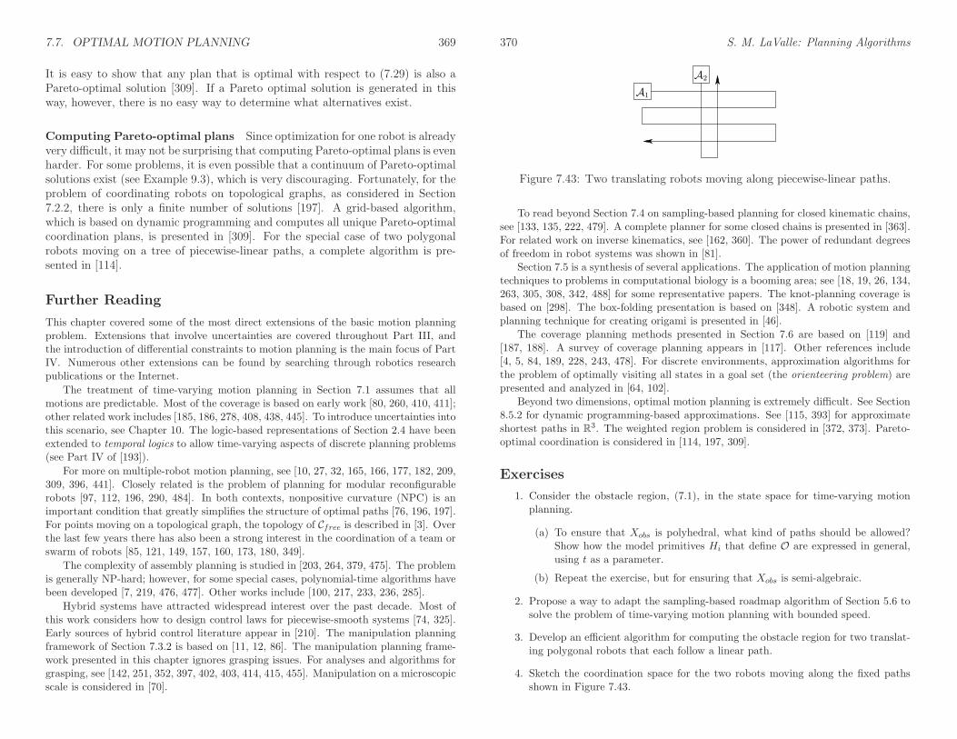
7.7. OPTIMAL MOTION PLANNING 369
It is easy to show that any plan that is optimal with respect to (7.29) is also aPareto-optimal solution [309]. If a Pareto optimal solution is generated in thisway, however, there is no easy way to determine what alternatives exist.
Computing Pareto-optimal plans Since optimization for one robot is alreadyvery difficult, it may not be surprising that computing Pareto-optimal plans is evenharder. For some problems, it is even possible that a continuum of Pareto-optimalsolutions exist (see Example 9.3), which is very discouraging. Fortunately, for theproblem of coordinating robots on topological graphs, as considered in Section7.2.2, there is only a finite number of solutions [197]. A grid-based algorithm,which is based on dynamic programming and computes all unique Pareto-optimalcoordination plans, is presented in [309]. For the special case of two polygonalrobots moving on a tree of piecewise-linear paths, a complete algorithm is pre-sented in [114].
Further Reading
This chapter covered some of the most direct extensions of the basic motion planningproblem. Extensions that involve uncertainties are covered throughout Part III, andthe introduction of differential constraints to motion planning is the main focus of PartIV. Numerous other extensions can be found by searching through robotics researchpublications or the Internet.
The treatment of time-varying motion planning in Section 7.1 assumes that allmotions are predictable. Most of the coverage is based on early work [80, 260, 410, 411];other related work includes [185, 186, 278, 408, 438, 445]. To introduce uncertainties intothis scenario, see Chapter 10. The logic-based representations of Section 2.4 have beenextended to temporal logics to allow time-varying aspects of discrete planning problems(see Part IV of [193]).
For more on multiple-robot motion planning, see [10, 27, 32, 165, 166, 177, 182, 209,309, 396, 441]. Closely related is the problem of planning for modular reconfigurablerobots [97, 112, 196, 290, 484]. In both contexts, nonpositive curvature (NPC) is animportant condition that greatly simplifies the structure of optimal paths [76, 196, 197].For points moving on a topological graph, the topology of Cfree is described in [3]. Overthe last few years there has also been a strong interest in the coordination of a team orswarm of robots [85, 121, 149, 157, 160, 173, 180, 349].
The complexity of assembly planning is studied in [203, 264, 379, 475]. The problemis generally NP-hard; however, for some special cases, polynomial-time algorithms havebeen developed [7, 219, 476, 477]. Other works include [100, 217, 233, 236, 285].
Hybrid systems have attracted widespread interest over the past decade. Most ofthis work considers how to design control laws for piecewise-smooth systems [74, 325].Early sources of hybrid control literature appear in [210]. The manipulation planningframework of Section 7.3.2 is based on [11, 12, 86]. The manipulation planning frame-work presented in this chapter ignores grasping issues. For analyses and algorithms forgrasping, see [142, 251, 352, 397, 402, 403, 414, 415, 455]. Manipulation on a microscopicscale is considered in [70].
370 S. M. LaValle: Planning Algorithms
A1
A2
Figure 7.43: Two translating robots moving along piecewise-linear paths.
To read beyond Section 7.4 on sampling-based planning for closed kinematic chains,see [133, 135, 222, 479]. A complete planner for some closed chains is presented in [363].For related work on inverse kinematics, see [162, 360]. The power of redundant degreesof freedom in robot systems was shown in [81].
Section 7.5 is a synthesis of several applications. The application of motion planningtechniques to problems in computational biology is a booming area; see [18, 19, 26, 134,263, 305, 308, 342, 488] for some representative papers. The knot-planning coverage isbased on [298]. The box-folding presentation is based on [348]. A robotic system andplanning technique for creating origami is presented in [46].
The coverage planning methods presented in Section 7.6 are based on [119] and[187, 188]. A survey of coverage planning appears in [117]. Other references include[4, 5, 84, 189, 228, 243, 478]. For discrete environments, approximation algorithms forthe problem of optimally visiting all states in a goal set (the orienteering problem) arepresented and analyzed in [64, 102].
Beyond two dimensions, optimal motion planning is extremely difficult. See Section8.5.2 for dynamic programming-based approximations. See [115, 393] for approximateshortest paths in R3. The weighted region problem is considered in [372, 373]. Pareto-optimal coordination is considered in [114, 197, 309].
Exercises
1. Consider the obstacle region, (7.1), in the state space for time-varying motionplanning.
(a) To ensure that Xobs is polyhedral, what kind of paths should be allowed?Show how the model primitives Hi that define O are expressed in general,using t as a parameter.
(b) Repeat the exercise, but for ensuring that Xobs is semi-algebraic.
2. Propose a way to adapt the sampling-based roadmap algorithm of Section 5.6 tosolve the problem of time-varying motion planning with bounded speed.
3. Develop an efficient algorithm for computing the obstacle region for two translat-ing polygonal robots that each follow a linear path.
4. Sketch the coordination space for the two robots moving along the fixed pathsshown in Figure 7.43.

7.7. OPTIMAL MOTION PLANNING 371
5. Suppose there are two robots, and each moves on its own roadmap of three paths.The paths in each roadmap are arranged end-to-end in a triangle.
(a) Characterize the fixed-roadmap coordination space that results, including adescription of its topology.
(b) Now suppose there are n robots, each on a triangular roadmap, and charac-terize the fixed-roadmap coordination space.
6. Consider the state space obtained as the Cartesian product of the C-spaces of nidentical robots. Suppose that each robot is labeled with a unique integer. Showthat X can be partitioned nicely into n! regions in which Xobs appears identicaland the only difference is the labels (which indicate the particular robots that arein collision).
7. Suppose there are two robots, and each moves on its own roadmap of three paths.The paths in one roadmap are arranged end-to-end in a triangle, and the pathsin the other are arranged as a Y. Characterize the fixed-roadmap coordinationspace that results, including a description of its topology.
8. Design an efficient algorithm that takes as input a graph representation of theconnectivity of a linkage and computes an active-passive decomposition. Assumethat all links are revolute. The algorithm should work for either 2D or 3D linkages(the dimension is also an input). Determine the asymptotic running time of youralgorithm.
9. Consider the problem of coordinating the motion of two robots that move alongprecomputed paths but in the presence of predictable moving obstacles. Developa planning algorithm for this problem.
10. Consider a manipulator in W = R2 made of four links connected in a chain byrevolute joints. There is unit distance between the joints, and the first joint isattached at (0, 0) in W = R2. Suppose that the end of the last link, which isposition (1, 0) in its body frame, is held at (0, 2) ∈ W.
(a) Use kinematics expressions to express the closure constraints for a configu-ration q ∈ C.
(b) Convert the closure constraints into polynomial form.
(c) Use differentiation to determine the constraints on the allowable velocitiesthat maintain closure at a configuration q ∈ C.
Implementations
11. Implement the vertical decomposition algorithm to solve the path-tuning problem,as shown in Figure 7.5.
12. Use grid-based sampling and a search algorithm to compute collision-free motionsof three robots moving along predetermined paths.
372 S. M. LaValle: Planning Algorithms
13. Under the conditions of Exercise 12, compute Pareto-optimal coordination strate-gies that optimize the time (number of stages) that each robot takes to reach itsgoal. Design a wavefront propagation algorithm that keeps track of the com-plete (ignoring equivalent strategies) set of minimal Pareto-optimal coordinationstrategies at each reached state. Avoid storing entire plans at each discretizedstate.
14. To gain an appreciation of the difficulties of planning for closed kinematic chains,try motion planning for a point on a torus among obstacles using only the implicittorus constraint given by (6.40). To simplify collision detection, the obstacles canbe a collection of balls in R3 that intersect the torus. Adapt a sampling-basedplanning technique, such as the bidirectional RRT, to traverse the torus and solveplanning problems.
15. Implement the spanning-tree coverage planning algorithm of Section 7.6.
16. Develop an RRT-based planning algorithm that causes the robot to chase anunpredictable moving target in a planar environment that contains obstacles.The algorithm should run quickly enough so that replanning can occur duringexecution. The robot should execute the first part of the most recently computedpath while simultaneously computing a better plan for the next time increment.
17. Modify Exercise 16 so that the robot assumes the target follows a predictable,constant-velocity trajectory until some deviation is observed.
18. Show how to handle unexpected obstacles by using a fast enough planning algo-rithm. For simplicity, suppose the robot is a point moving in a polygonal obstacleregion. The robot first computes a path and then starts to execute it. If theobstacle region changes, then a new path is computed from the robot’s currentposition. Use vertical decomposition or another algorithm of your choice (pro-vided it is fast enough). The user should be able to interactively place or moveobstacles during plan execution.
19. Use the manipulation planning framework of Section 7.3.2 to develop an algorithmthat solves the famous Towers of Hanoi problem by a robot that carries the rings[86]. For simplicity, suppose a polygonal robot moves polygonal parts in W = R2
and rotation is not allowed. Make three pegs, and initially place all parts onone peg, sorted from largest to smallest. The goal is to move all of the parts toanother peg while preserving the sorting.
20. Use grid-based approximation to solve optimal planning problems for a pointrobot in the plane. Experiment with using different neighborhoods and metrics.Characterize the combinations under which good and bad approximations areobtained.

Chapter 8
Feedback Motion Planning
So far in Part II it has been assumed that a continuous path sufficiently solvesa motion planning problem. In many applications, such as computer-generatedanimation and virtual prototyping, there is no need to challenge this assumptionbecause models in a virtual environment usually behave as designed. In applica-tions that involve interaction with the physical world, future configurations maynot be predictable. A traditional way to account for this in robotics is to use therefinement scheme that was shown in Figure 1.19 to design a feedback control lawthat attempts to follow the computed path as closely as possible. Sometimes thisis satisfactory, but it is important to recognize that this approach is highly de-coupled. Feedback and dynamics are neglected in the construction of the originalpath; the computed path may therefore not even be usable.
Section 8.1 motivates the consideration of feedback in the context of motionplanning. Section 8.2 presents the main concepts of this chapter, but only for thecase of a discrete state space. This requires less mathematical concepts than thecontinuous case, making it easier to present feedback concepts. Section 8.3 thenprovides the mathematical background needed to extend the feedback conceptsto continuous state spaces (which includes C-spaces). Feedback motion planningmethods are divided into complete methods, covered in Section 8.4, and sampling-based methods, covered in Section 8.5.
8.1 Motivation
For most problems involving the physical world, some form of feedback is needed.This means the actions of a plan should depend in some way on informationgathered during execution. The need for feedback arises from the unpredictabilityof future states. In this chapter, every state space will be either discrete, orX = C,which is a configuration space as considered in Chapter 4.
Two general ways to model uncertainty in the predictability of future statesare
1. Explicitly: Develop models that explicitly account for the possible ways
373
374 S. M. LaValle: Planning Algorithms
Open Loop FeedbackFree motions Traditional motion planning Chapter 8
Dynamics Chapters 14 and 15 Traditional control theory
Figure 8.1: By separating the issue of dynamics from feedback, two less-investigated topics emerge.
that the actual future state can drift away from the planned future state. Aplanning algorithm must take this uncertainty directly into account. Suchexplicit models of uncertainty are introduced and incorporated into the plan-ning model in Part III.
2. Implicitly: The model of state transitions indicates that no uncertainty ispossible; however, a feedback plan is constructed to ensure that it knowswhich action to apply, just in case it happens to be in some unexpectedstate during execution. This approach is taken in this chapter.
The implicit way to handle this uncertainty may seem strange at first; therefore,some explanation is required. It will be seen in Part III that explicitly mod-eling uncertainty is extremely challenging and complicated. The requirementsfor expressing reliable models are much stronger; the complexity of the problemincreases, making algorithm design more difficult and leading to greater opportu-nities to make modeling errors. The implicit way of handling uncertainty in pre-dictability arose in control theory [63, 66, 356]. It is well known that a feedbackcontrol law is needed to obtain reliable performance, yet it is peculiar that the for-mulation of dynamics used in most contexts does not explicitly account for this.Classical control theory has always assumed that feedback is crucial; however,only in modern branches of the field, such as stochastic control and robust control,does this uncertainty get explicitly modeled. Thus, there is a widely accepted andsuccessful practice of designing feedback control laws that use state feedback toimplicitly account for the fact that future states may be unpredictable. Given thewidespread success of this control approach across numerous applications over thepast century, it seems valuable to utilize this philosophy in the context of motionplanning as well (if you still do not like it, then jump to Chapter 10).
Due to historical reasons in the development of feedback control, it often seemsthat feedback and dynamics are inseparable. This is mainly because control theorywas developed to reliably alter the behavior of dynamical systems. In traditionalmotion planning, neither feedback nor dynamics is considered. A solution pathis considered open loop, which means there is no feedback of information duringexecution to close the loop. Dynamics are also not handled because the additionalcomplications of differential constraints and higher dimensional phase spaces arise(see Part IV).
By casting history aside and separating feedback from dynamics, four separatetopics can be made, as shown in Figure 8.1. The topic of open-loop planning that

8.2. DISCRETE STATE SPACES 375
involves dynamics has received increasing attention in recent years. This is thefocus throughout most of Part IV. Those fond of classical control theory maycriticize it for failing to account for feedback; however, such open-loop trajectories(paths in a phase space) are quite useful in applications that involve simulations.Furthermore, a trajectory that accounts for dynamics is more worthwhile in adecoupled approach than using a path that ignores dynamics, which has been anacceptable practice for decades. These issues will be elaborated upon further inPart IV.
The other interesting topic that emerges in Figure 8.1 is to develop feedbackplans for problems in which there are no explicit models of dynamics or otherdifferential constraints. If it was reasonable to solve problems in classical motionplanning by ignoring differential constraints, one should certainly feel no less guiltydesigning feedback motion plans that still neglect differential constraints.1 Thisuses the implicit model of uncertainty in predictability without altering any of theother assumptions previously applied in traditional motion planning.
Even if there are no unpredictability issues, another important use of feedbackplans is for problems in which the initial state is not known. A feedback planindicates what action to take from every state. Therefore, the specification ofan initial condition is not important. The analog of this in graph algorithms isthe single-destination shortest-path problem, which indicates how to arrive at aparticular vertex optimally from any other vertex. Due to this connection, thenext section presents feedback concepts for discrete state spaces, before extendingthe ideas to continuous spaces, which are needed for motion planning.
For these reasons, feedback motion planning is considered in this chapter. Asa module in a decoupled approach used in robotics, feedback motion plans are atleast as useful as a path computed by the previous techniques. We expect feedbacksolutions to be more reliable in general, when used in the place of open-loop pathscomputed by traditional motion planning algorithms.
8.2 Discrete State Spaces
This section is provided mainly to help to explain similar concepts that are comingin later sections. The presentation is limited to discrete spaces, which are muchsimpler to formulate and understand. Following this, an extension to configurationspaces and other continuous state spaces can be made. The discussion here is alsorelevant background for the feedback planning concepts that will be introduced inSection 8.4.1. In that case, uncertainty will be explicitly modeled. The resultingformulation and concepts can be considered as an extension of this section.
1Section 8.4.4 will actually consider some simple differential constraints, such as accelerationbounds; the full treatment of differential constraints is deferred until Part IV.
376 S. M. LaValle: Planning Algorithms
8.2.1 Defining a Feedback Plan
Consider a discrete planning problem similar to the ones defined in Formulations2.1 and 2.3, except that the initial state is not given. Due to this, the costfunctional cannot be expressed only as a function of a plan. It is instead definedin terms of the state history and action history. At stage k, these are defined as
xk = (x1, x2, . . . , xk) (8.1)
anduk = (u1, u2, . . . , uk), (8.2)
respectively. Sometimes, it will be convenient to alternatively refer to xk as thestate trajectory.
The resulting formulation is
Formulation 8.1 (Discrete Optimal Feedback Planning)
1. A finite, nonempty state space X.
2. For each state, x ∈ X, a finite action space U(x).
3. A state transition function f that produces a state, f(x, u) ∈ X, for everyx ∈ X and u ∈ U(x). Let U denote the union of U(x) for all x ∈ X.
4. A set of stages, each denoted by k, that begins at k = 1 and continuesindefinitely.
5. A goal set, XG ⊂ X.
6. Let L denote a stage-additive cost functional,
L(xF , uK) =K∑
k=1
l(xk, uk) + lF (xF ), (8.3)
in which F = K + 1.
There is one other difference in comparison to the formulations of Chapter 2. Thestate space is assumed here to be finite. This facilitates the construction of afeedback plan, but it is not necessary in general.
Consider defining a plan that solves Formulation 8.1. If the initial conditionis given, then a sequence of actions could be specified, as in Chapter 2. Withouthaving the initial condition, one possible approach is to determine a sequence ofactions for each possible initial state, x1 ∈ X. Once the initial state is given, theappropriate action sequence is known. This approach, however, wastes memory.Suppose some x is given as the initial state and the first action is applied, leadingto the next state x′. What action should be applied from x′? The second actionin the sequence at x can be used; however, we can also imagine that x′ is now the

8.2. DISCRETE STATE SPACES 377
initial state and use its first action. This implies that keeping an action sequencefor every state is highly redundant. It is sufficient at each state to keep only thefirst action in the sequence. The application of that action produces the nextstate, at which the next appropriate action is stored. An execution sequence canbe imagined from an initial state as follows. Start at some state, apply the actionstored there, arrive at another state, apply its action, arrive at the next state, andso on, until the goal is reached.
It therefore seems appropriate to represent a feedback plan as a function thatmaps every state to an action. Therefore, a feedback plan π is defined as a functionπ : X → U . From every state, x ∈ X, the plan indicates which action to apply.If the goal is reached, then the termination action should be applied. This isspecified as part of the plan: π(x) = uT , if x ∈ XG. A feedback plan is called asolution to the problem if it causes the goal to be reached from every state thatis reachable from the goal.
If an initial state x1 and a feedback plan π are given, then the state and actionhistories can be determined. This implies that the execution cost, (8.3), also canbe determined. It can therefore be alternatively expressed as L(π, x1), instead ofL(xF , uK). This relies on future states always being predictable. In Chapter 10,it will not be possible to make this direct correspondence due to uncertainties (seeSection 10.1.3).
Feasibility and optimality The notions of feasible and optimal plans need tobe reconsidered in the context of feedback planning because the initial conditionis not given. A plan π is called a solution to the feasible planning problem iffrom every x ∈ X from which XG is reachable the goal set is indeed reached byexecuting π from x. This means that the cost functional is ignored (an alternativeto Formulation 8.1 can be defined in which the cost functional is removed). Forconvenience, π will be called a feasible feedback plan.
Now consider optimality. From a given state x, it is clear that an optimal planexists using the concepts of Section 2.3. Is it possible that a different optimal planneeds to be associated with every x ∈ X that can reach XG? It turns out thatonly one plan is needed to encode optimal paths from every initial state to XG.Why is this true? Suppose that the optimal cost-to-go is computed over X usingDijkstra’s algorithm or value iteration, as covered in Section 2.3. Every cost-to-go value at some x ∈ X indicates the cost received under the implementationof the optimal open-loop plan from x. The first step in this optimal plan canbe determined by (2.19), which yields a new state x′ = f(x, u). From x′, (2.19)can be applied once again to determine the next optimal action. The cost at x′
represents both the optimal cost-to-go if x′ is the initial condition and also theoptimal cost-to-go when continuing on the optimal path from x. The two mustbe equivalent because of the dynamic programming principle. Since all such costsmust coincide, a single feedback plan can be used to obtain the optimal cost-to-gofrom every initial condition.
378 S. M. LaValle: Planning Algorithms
xG uT
(a) (b)
Figure 8.2: a) A 2D grid-planning problem. b) A solution feedback plan.
A feedback plan π is therefore defined as optimal if from every x ∈ X, the totalcost, L(π, x), obtained by executing π is the lowest among all possible plans. Therequirement that this holds for every initial condition is important for feedbackplanning.
Example 8.1 (Feedback Plan on a 2D Grid) This example uses the 2D gridmodel explained in Example 2.1. A robot moves on a grid, and the possible actionsare up (↑), down (↓), left (←), right (→), and terminate (uT ); some directionsare not available from some states. A solution feedback plan is depicted in Figure8.2. Many other possible solutions plans exist. The one shown here happens tobe optimal in terms of the number of steps to the goal. Some alternative feedbackplans are also optimal (figure out which arrows can be changed). To apply theplan from any initial state, simply follow the arrows to the goal. In each stage,the application of the action represented by the arrow leads to the next state. Theprocess terminates when uT is applied at the goal.
8.2.2 Feedback Plans as Navigation Functions
It conveniently turns out that tools for computing a feedback plan were alreadygiven in Chapter 2. Methods such as Dijkstra’s algorithm and value iterationproduce information as a side effect that can be used to represent a feedbackplan. This section explains how this information is converted into a feedbackplan. To achieve this, a feedback plan will be alternatively expressed as a potentialfunction over the state space (recall potential functions from Section 5.4.3). The
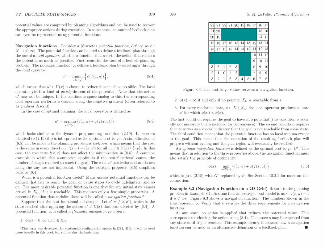
8.2. DISCRETE STATE SPACES 379
potential values are computed by planning algorithms and can be used to recoverthe appropriate actions during execution. In some cases, an optimal feedback plancan even be represented using potential functions.
Navigation functions Consider a (discrete) potential function, defined as φ :X → [0,∞]. The potential function can be used to define a feedback plan throughthe use of a local operator, which is a function that selects the action that reducesthe potential as much as possible. First, consider the case of a feasible planningproblem. The potential function, φ, defines a feedback plan by selecting u throughthe local operator,
u∗ = argminu∈U(x)
φ(f(x, u))
, (8.4)
which means that u∗ ∈ U(x) is chosen to reduce φ as much as possible. The localoperator yields a kind of greedy descent of the potential. Note that the actionu∗ may not be unique. In the continuous-space analog to this, the correspondinglocal operator performs a descent along the negative gradient (often referred toas gradient descent).
In the case of optimal planning, the local operator is defined as
u∗ = argminu∈U(x)
l(x, u) + φ(f(x, u))
, (8.5)
which looks similar to the dynamic programming condition, (2.19). It becomesidentical to (2.19) if φ is interpreted as the optimal cost-to-go. A simplification of(8.5) can be made if the planning problem is isotropic, which means that the costis the same in every direction: l(x, u) = l(x, u′) for all u, u′ ∈ U(x) \ uT. In thiscase, the cost term l(x, u) does not affect the minimization in (8.5). A commonexample in which this assumption applies is if the cost functional counts thenumber of stages required to reach the goal. The costs of particular actions chosenalong the way are not important. Using the isotropic property, (8.5) simplifiesback to (8.4).
When is a potential function useful? Many useless potential functions can bedefined that fail to reach the goal, or cause states to cycle indefinitely, and soon. The most desirable potential function is one that for any initial state causesarrival in XG, if it is reachable. This requires only a few simple properties. Apotential function that satisfies these will be called a navigation function.2
Suppose that the cost functional is isotropic. Let x′ = f(x, u∗), which is thestate reached after applying the action u∗ ∈ U(x) that was selected by (8.4). Apotential function, φ, is called a (feasible) navigation function if
1. φ(x) = 0 for all x ∈ XG.
2This term was developed for continuous configuration spaces in [284, 416]; it will be usedmore broadly in this book but still retains the basic idea.
380 S. M. LaValle: Planning Algorithms
1
1
1
1
2 2
22
2 2
3 3
3 3 4 5 6 7
7 8
8
8
9
9
9
10
10
10
11
11
11
0
12
12
12
12
13
13
13
1314
14
14
14
15
15
15
15 16
16
16
1617
17
17 17
18
18
18
19
19
19
20
20
2021
21 212222
Figure 8.3: The cost-to-go values serve as a navigation function.
2. φ(x) =∞ if and only if no point in XG is reachable from x.
3. For every reachable state, x ∈ X \XG, the local operator produces a statex′ for which φ(x′) < φ(x).
The first condition requires the goal to have zero potential (this condition is actu-ally not necessary but is included for convenience). The second condition requiresthat∞ serves as a special indicator that the goal is not reachable from some state.The third condition means that the potential function has no local minima exceptat the goal. This means that the execution of the resulting feedback plan willprogress without cycling and the goal region will eventually be reached.
An optimal navigation function is defined as the optimal cost-to-go, G∗. Thismeans that in addition to the three properties above, the navigation function mustalso satisfy the principle of optimality:
φ(x) = minu∈U(x)
l(x, u) + φ(f(x, u))
, (8.6)
which is just (2.18) with G∗ replaced by φ. See Section 15.2.1 for more on thisconnection.
Example 8.2 (Navigation Function on a 2D Grid) Return to the planningproblem in Example 8.1. Assume that an isotropic cost model is used: l(x, u) = 1if u 6= uT . Figure 8.3 shows a navigation function. The numbers shown in thetiles represent φ. Verify that φ satisfies the three requirements for a navigationfunction.
At any state, an action is applied that reduces the potential value. Thiscorresponds to selecting the action using (8.4). The process may be repeated fromany state until XG is reached. This example clearly illustrates how a navigationfunction can be used as an alternative definition of a feedback plan.

8.2. DISCRETE STATE SPACES 381
Example 8.3 (Airport Terminal) You may have found yourself using a nav-igation function to find the exit after arriving in an unfamiliar airport terminal.Many terminals are tree-structured, with increasing gate numbers as the distanceto the terminal exit increases. If you wish to leave the terminal, you should nor-mally walk toward the lower numbered gates.
Computing navigation functions There are many ways to compute naviga-tion functions. The cost-to-go function determined by Dijkstra’s algorithm work-ing backward from XG yields an optimal navigation function. The third conditionof a navigation function under the anisotropic case is exactly the stationary dy-namic programming equation, (2.18), if the navigation function φ is defined as theoptimal cost-to-go G∗. It was mentioned previously that the optimal actions canbe recovered using only the cost-to-go. This was actually an example of using anavigation function, and the resulting procedure could have been considered as afeedback plan.
If optimality is not important, then virtually any backward search algorithmfrom Section 2.2 can be used, provided that it records the distance to the goalfrom every reached state. The distance does not have to be optimal. It merelycorresponds to the cost obtained if the current vertex in the search tree is tracedback to the root vertex (or back to any vertex in XG, if there are multiple goalstates).
If the planning problem does not even include a cost functional, as in Formu-lation 2.1, then a cost functional can be invented for the purposes of constructinga navigation function. At each x ∈ X from which XG is reachable, the numberof edges in the search graph that would be traversed from x to XG can be storedas the cost. If Dijkstra’s algorithm is used to construct the navigation function,then the resulting feedback plan yields executions that are shortest in terms ofthe number of stages required to reach the goal.
The navigation function itself serves as the representation of the feedbackplan, by recovering the actions from the local operator. Thus, a function, π :X → U , can be recovered from a navigation function, φ : X → [0,∞]. Likewise,a navigation function, φ, can be constructed from π. Therefore, the π and φ canbe considered as interchangeable representations of feedback plans.
8.2.3 Grid-Based Navigation Functions for Motion Plan-ning
To consider feedback plans for continuous spaces, vector fields and other basicdefinitions from differential geometry will be needed. These will be covered inSection 8.3; however, before handling such complications, we first will describehow to use the ideas presented so far in Section 8.2 as a discrete approximationto feedback motion planning.
382 S. M. LaValle: Planning Algorithms
WAVEFRONT PROPAGATION ALGORITHM
1. Initialize W0 = XG; i = 0.
2. Initialize Wi+1 = ∅.
3. For every x ∈ Wi, assign φ(x) = i and insert all unexplored neighbors of xinto Wi+1.
4. If Wi+1 = ∅, then terminate; otherwise, let i := i+ 1 and go to Step 2.
Figure 8.4: The wavefront propagation algorithm is a specialized version of Dijk-stra’s algorithm that optimizes the number of stages to reach the goal.
Examples 8.1 and 8.2 have already defined feedback plans and navigation func-tions for 2D grids that contain obstacles. Imagine that this model is used to ap-proximate a motion planning problem for which C ⊂ R2. Section 5.4.2 showedhow to make a topological graph that approximates the motion planning prob-lem with a grid of samples. The motions used in Example 8.1 correspond to the1-neighborhood definition, (5.37). This idea was further refined in Section 7.7.1to model approximate optimal motion planning by moving on a grid; see Formu-lation 7.4. By choosing the Manhattan motion model, as defined in Example 7.4,a grid with the same motions considered in Example 8.1 is produced.
To construct a navigation function that may be useful in mobile robotics, ahigh-resolution (e.g., 50 to 100 points per axis) grid is usually required. In Section5.4.2, only a few points per axis were needed because feedback was not assumed.It was possible in some instances to find a collision-free path by investigating onlya few points per axis. During the execution of a feedback plan, it is assumedthat the future states of the robot are not necessarily predictable. Wherever therobot may end up, the navigation function in combination with the local operatormust produce the appropriate action. If the current state (or configuration) isapproximated by a grid, then it is important to reduce the approximation erroras much as possible. This is accomplished by setting the grid resolution high. Inthe feedback case, the grid can be viewed as “covering” the whole configurationspace, whereas in Section 5.4.2 the grid only represented a topological graph ofpaths that cut across the space.3
Wavefront propagation algorithms Once the approximation has been made,any of the methods discussed in Section 8.2.2 can be used to compute a navigationfunction. An optimal navigation function can be easily computed using Dijkstra’s
3Difficulty in distinguishing between these two caused researchers for many years to believethat grids yield terrible performance for the open-loop path planning problems of Chapter 5.This was mainly because it was assumed that a high-resolution grid was necessary. For manyproblems, however, they could terminate early after only considering a few points per axis.

8.2. DISCRETE STATE SPACES 383
algorithm from the goal. If each motion has unit cost, then a useful simplificationcan be made. Figure 8.4 describes a wavefront propagation algorithm that com-putes an optimal navigation function. It can be considered as a special case ofDijkstra’s algorithm that avoids explicit construction of the priority queue. In Di-jkstra’s algorithm, the cost of the smallest element in the queue is monotonicallynondecreasing during the execution of the algorithm. In the case of each motionhaving unit cost, there will be many states in the queue that have the same cost.Dijkstra’s algorithm could remove in parallel all elements that have the same,smallest cost. Suppose the common, smallest cost value is i. These states areorganized into a wavefront, Wi. The initial wavefront is W0, which represents thestates in XG. The algorithm can immediately assign an optimal cost-to-go valueof 1 to every state that can be reached in one stage from any state in W0. Thesemust be optimal because no other cost value is optimal. The states that receivecost 1 can be organized into the wavefront W1. The unexplored neighbors of W1
are assigned cost 2, which also must be optimal. This process repeats inductivelyfrom i to i+1 until all reachable states have been reached. In the end, the optimalcost-to-go is computed in O(n) time, in which n is the number of reachable gridstates. For any states that were not reached, the value φ(x) =∞ can be assigned.The navigation function shown in Figure 8.3 can actually be computed using thewavefront propagation algorithm.
Maximum clearance One problem that typically arises in mobile robotics isthat optimal motion plans bring robots too close to obstacles. Recall from Section6.2.4 that the shortest Euclidean paths for motion planning in a polygonal envi-ronment must be allowed to touch obstacle vertices. This motivated the maximumclearance roadmap, which was covered in Section 6.2.3. A grid-based approximateversion of the maximum clearance roadmap can be made. Furthermore, a naviga-tion function can be defined that guides the robot onto the roadmap, then travelsalong the roadmap, and finally deposits the robot at a specified goal. In [304], theresulting navigation function is called NF2.
Assume that there is a single goal state, xG ∈ X. The computation of amaximum clearance navigation function proceeds as follows:
1. Instead of XG, assign W0 to be the set of all states from which motion in atleast one direction is blocked. These are the states on the boundary of thediscretized collision-free space.
2. Perform wavefront iterations that propagate costs in waves outward fromthe obstacle boundaries.
3. As the wavefronts propagate, they will meet approximately at the location ofthe maximum clearance roadmap for the original, continuous problem. Markany state at which two wavefront points arrive from opposing directions asa skeleton state. It may be the case that the wavefronts simply touch each
384 S. M. LaValle: Planning Algorithms
other, rather than arriving at a common state; in this case, one of the twotouching states is chosen as the skeleton state. Let S denote the set of allskeleton states.
4. After the wavefront propagation ends, connect xG to the skeleton by insert-ing xG and all states along the path to the skeleton into S. This path canbe found using any search algorithm.
5. Compute a navigation function φ1 over S by treating all other states as ifthey were obstacles and using the wavefront propagation algorithm. Thisnavigation function guides any point in S to the goal.
6. Treat S as a goal region and compute a navigation function φ2 using thewavefront propagation algorithm. This navigation function guides the stateto the nearest point on the skeleton.
7. Combine φ1 and φ2 as follows to obtain φ. For every x ∈ S, let φ(x) = φ1(x).For every remaining state, the value φ(x) = φ1(x
′) + φ2(x) is assigned, inwhich x′ is the nearest state to x such that x′ ∈ S. The state x′ can easilybe recorded while φ2 is computed.
If Cfree is multiply connected, then there may be multiple ways to each xG bytraveling around different obstacles (the paths are not homotopic). The methoddescribed above does not take into account the problem that one route may havea tighter clearance than another. The given approach only optimizes the distancetraveled along the skeleton; it does not, however, maximize the nearest approachto an obstacle, if there are multiple routes.
Dial’s algorithm Now consider generalizing the wavefront propagation idea.Wavefront propagation can be applied to any discrete planning problem if l(x, u) =1 for any x ∈ X and u ∈ U(x) (except u = uT ). It is most useful when thetransition graph is sparse (imagine representing the transition graph using anadjacency matrix). The grid problem is a perfect example where this becomesimportant. More generally, if the cost terms assume integer values, then Dial’salgorithm [148] results, which is a generalization of wavefront propagation, anda specialization of Dijkstra’s algorithm. The idea is that the priority queue canbe avoided by assigning the alive vertices to buckets that correspond to differentpossible cost-to-go values. In the wavefront propagation case, there are nevermore than two buckets needed at a time. Dial’s algorithm allows all states in thesmallest cost bucket to be processed in parallel. The scheme was enhanced in[460] to yield a linear-time algorithm.
Other extensions Several ideas from this section can be generalized to produceother navigation functions. One disadvantage of the methods discussed so far isthat undesirable staircase motions (as shown in Figure 7.40) are produced. If the

8.3. VECTOR FIELDS AND INTEGRAL CURVES 385
2-neighborhood, as defined in (5.38), is used to define the action spaces, then themotions will generally be shorter. Dial’s algorithm can be applied to efficientlycompute an optimal navigation function in this case.
A grid approximation can be made to higher dimensional configuration spaces.Since a high resolution is needed, however, it is practical only for a few dimensions(e.g., 3 or 4). If the 1-neighborhood is used, then wavefront propagation can beeasily applied to compute navigation functions. Dial’s algorithm can be adaptedfor general k-neighborhoods.
Constructing navigation functions over grids may provide a practical solutionin many applications. In other cases it may be unacceptable that staircase motionsoccur. In many cases, it may not even be possible to compute the navigationfunction quickly enough. Factors that influence this problem are 1) very highaccuracy, and a hence high-resolution grid may be necessary; 2) the dimension ofthe configuration space may be high; and 3) the environment may be frequentlychanging, and a real-time response is required. To address these issues, it isappealing to abandon grid approximations. This will require defining potentialfunctions and velocities directly on the configuration space. Section 8.3 presentsthe background mathematical concepts to make this transition.
8.3 Vector Fields and Integral Curves
To consider feedback motion plans over continuous state spaces, including con-figuration spaces, we will need to define a vector field and the trajectory that isobtained by integrating the vector field from an initial point. A vector field isideal for characterizing a feedback plan over a continuous state space. It can beviewed as providing the continuous-space analog to the feedback plans on grids,as shown in Figure 8.2b.
This section presents two alternative presentations of the background mathe-matical concepts. Section 8.3.1 assumes that X = Rn, which leads to definitionsthat appear very similar to those you may have learned in basic calculus and dif-ferential equations courses. Section 8.3.2 covers the more general case of vectorfields on manifolds. This requires significantly more technical concepts and buildson the manifold definitions of Section 4.1.2.
Some readers may have already had some background in differentiable man-ifolds. If, however, you are seeing it for the first time, then it may be difficultto comprehend on the first reading. In addition to rereading, here are two othersuggestions. First, try studying background material on this subject, which issuggested at the end of the chapter. Second, disregard the manifold technicalitiesin the subsequent sections and pretend that X = C = Rn. Nearly everything willmake sense without the additional technicalities. Imagine that a manifold is de-fined as a cube, [0, 1]n, with some sides identified, as in Section 4.1.2. The conceptsthat were presented for Rn can be applied everywhere except at the boundary ofthe cube. For example, if S1 is defined as [0, 1]/ ∼, and a function f is defined on
386 S. M. LaValle: Planning Algorithms
S1, how can we define the derivative at f(0)? The technical definitions of Section8.3.2 fix this problem. Sometimes, the technicalities can be avoided in practice bycleverly handling the identification points.
8.3.1 Vector Fields on Rn
This section revisits some basic concepts from introductory courses such as calcu-lus, linear algebra, and differential equations. You may have learned most of thesefor R2 and R3. We eventually want to describe velocities in Rn and on manifolds,and then use the notion of a vector field to express a feedback plan in Section8.4.1.
Vector spaces Before defining a vector field, it is helpful to be precise aboutwhat is meant by a vector. A vector space (or linear space) is defined as a set,V , that is closed under two algebraic operations called vector addition and scalarmultiplication and satisfies several axioms, which will be given shortly. The vectorspace used in this section is Rn, in which the scalars are real numbers, and a vectoris represented as a sequence of n real numbers. Scalar multiplication multiplieseach component of the vector by the scalar value. Vector addition forms a newvector by adding each component of two vectors.
A vector space V can be defined over any field F (recall the definition fromSection 4.4.1). The field F represents the scalars, and V represents the vectors.The concepts presented below generalize the familiar case of the vector space Rn.In this case, V = Rn and F = R. In the definitions that follow, you may makethese substitutions, if desired. We will not develop vector spaces that are moregeneral than this; the definitions are nevertheless given in terms of V and F toclearly separate scalars from vectors. The vector addition is denoted by +, and thescalar multiplication is denoted by ·. These operations must satisfy the followingaxioms (a good exercise is to verify these for the case of Rn treated as a vectorspace over the field R):
1. (Commutative Group Under Vector Addition) The set V is a com-mutative group with respect to vector addition, +.
2. (Associativity of Scalar Multiplication) For any v ∈ V and any α, β ∈F, α(βv) = (αβ)v.
3. (Distributivity of Scalar Sums) For any v ∈ V and any α, β ∈ F, (α +β)v = αv + βv.
4. (Distributivity of Vector Sums) For any v, w ∈ V and any α ∈ F,α(v + w) = αv + αw.
5. (Scalar Multiplication Identity) For any v ∈ V , 1v = v for the multi-plicative identity 1 ∈ F.

8.3. VECTOR FIELDS AND INTEGRAL CURVES 387
The first axiom allows vectors to be added in any order. The rest of the axiomsrequire that the scalar multiplication interacts with vectors in the way that wewould expect from the familiar vector space Rn over R.
A basis of a vector space V is defined as a set, v1,. . .,vn, of vectors for whichevery v ∈ V can be uniquely written as a linear combination:
v = α1v1 + α2v2 + · · ·+ αnvn, (8.7)
for some α1, . . . , αn ∈ F. This means that every vector has a unique representationas a linear combination of basis elements. In the case of R3, a familiar basis is[0 0 1], [0 1 0], and [1 0 0]. All vectors can be expressed as a linear combinationof these three. Remember that a basis is not necessarily unique. From linearalgebra, recall that any three linearly independent vectors can be used as a basisfor R3. In general, the basis must only include linearly independent vectors. Eventhough a basis is not necessarily unique, the number of vectors in a basis is thesame for any possible basis over the same vector space. This number, n, is calledthe dimension of the vector space. Thus, we can call Rn an n-dimensional vectorspace over R.
Example 8.4 (The Vector Space Rn Over R) As indicated already, Rn canbe considered as a vector space. A natural basis is the set of n vectors in which,for each i ∈ 1, . . . , n, a unit vector is constructed as follows. Let xi = 1 andxj = 0 for all j 6= i. Since there are n basis vectors, Rn is an n-dimensional vectorspace. The basis is not unique. Any set of n linearly independent vectors may beused, which is familiar from linear algebra, in which nonsingular n × n matricesare used to transform between them.
To illustrate the power of these general vector space definitions, consider thefollowing example.
Example 8.5 (A Vector Space of Functions) The set of all continuous, real-valued functions f : [0, 1]→ R, for which
∫ 1
0
f(x)dx (8.8)
is finite, forms a vector space over R. It is straightforward to verify that the vectorspace axioms are satisfied. For example, if two functions f1 and f2 are added, theintegral remains finite. Furthermore, f1+f2 = f2+f1, and all of the group axiomsare satisfied with respect to addition. Any function f that satisfies (8.8) can bemultiplied by a scalar in R, and the integral remains finite. The axioms thatinvolve scalar multiplication can also be verified.
It turns out that this vector space is infinite-dimensional. One way to see this isto restrict the functions to the set of all those for which the Taylor series exists and
388 S. M. LaValle: Planning Algorithms
converges to the function (these are called analytic functions). Each function canbe expressed via a Taylor series as a polynomial that may have an infinite numberof terms. The set of all monomials, x, x2, x3, and so on, represents a basis. Everycontinuous function can be considered as an infinite vector of coefficients; eachcoefficient is multiplied by one of the monomials to produce the function. Thisprovides a simple example of a function space; with some additional definitions,this leads to a Hilbert space, which is crucial in functional analysis, a subject thatcharacterizes spaces of functions [420, 422].
The remainder of this chapter considers only finite-dimensional vector spacesover R. It is important, however, to keep in mind the basic properties of vectorspaces that have been provided.
Vector fields A vector field looks like a “needle diagram” over Rn, as depictedin Figure 8.5. The idea is to specify a direction at each point p ∈ Rn. When usedto represent a feedback plan, it indicates the direction that the robot needs tomove if it finds itself at p.
For every p ∈ Rn, associate an n-dimensional vector space called the tangentspace at p, which is denoted as Tp(R
n). Why not just call it a vector space atp? The use of the word “tangent” here might seem odd; it is motivated by thegeneralization to manifolds, for which the tangent spaces will be “tangent” topoints on the manifold.
A vector field4 ~V on Rn is a function that assigns a vector v ∈ Tp(Rn) to every
p ∈ Rn. What is the range of this function? The vector ~V (p) at each p ∈ Rn
actually belongs to a different tangent space. The range of the function is thereforethe union
T (Rn) =⋃
p∈Rn
Tp(Rn), (8.9)
which is called the tangent bundle on Rn. Even though the way we describe vectorsfrom Tp(R
n) may appear the same for any p ∈ Rn, each tangent space is assumed toproduce distinct vectors. To maintain distinctness, a point in the tangent bundlecan be expressed with 2n coordinates, by specifying p and v together. This willbecome important for defining phase space concepts in Part IV. In the presentsetting, it is sufficient to think of the range of ~V as Rn because Tp(R
n) = Rn forevery p ∈ Rn.
A vector field can therefore be expressed using n real-valued functions on Rn.Let fi(x1, . . . , xn) for i from 1 to n denote such functions. Using these, a vectorfield is specified as
f(x) = [f1(x1, . . . , xn) f2(x1, . . . , xn) · · · fn(x1, . . . , xn)]. (8.10)
4Unfortunately, the term field appears in two unrelated places: in the definition of a vectorspace and in the term vector field. Keep in mind that this is an accidental collision of terms.
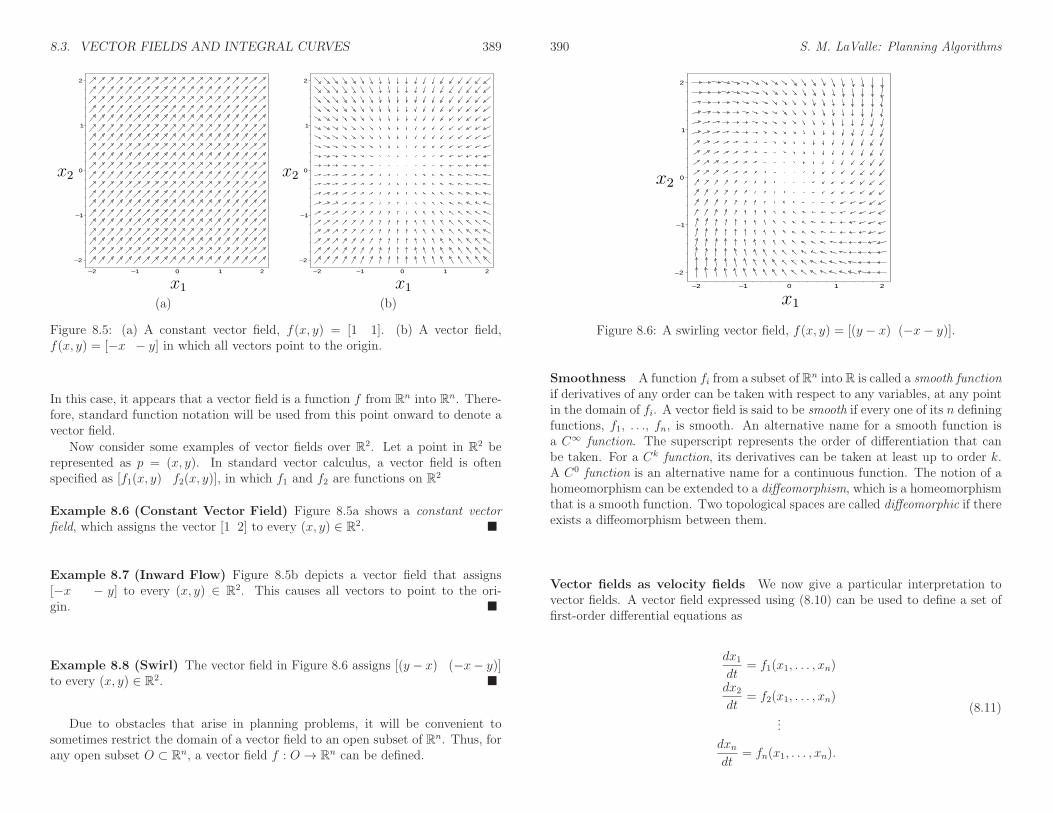
8.3. VECTOR FIELDS AND INTEGRAL CURVES 389
–2
–1
0
1
2
x_2
–2 –1 0 1 2
x_1
x2
x1
–2
–1
0
1
2
x_2
–2 –1 0 1 2
x_1
x2
x1
(a) (b)
Figure 8.5: (a) A constant vector field, f(x, y) = [1 1]. (b) A vector field,f(x, y) = [−x − y] in which all vectors point to the origin.
In this case, it appears that a vector field is a function f from Rn into Rn. There-fore, standard function notation will be used from this point onward to denote avector field.
Now consider some examples of vector fields over R2. Let a point in R2 berepresented as p = (x, y). In standard vector calculus, a vector field is oftenspecified as [f1(x, y) f2(x, y)], in which f1 and f2 are functions on R2
Example 8.6 (Constant Vector Field) Figure 8.5a shows a constant vectorfield, which assigns the vector [1 2] to every (x, y) ∈ R2.
Example 8.7 (Inward Flow) Figure 8.5b depicts a vector field that assigns[−x − y] to every (x, y) ∈ R2. This causes all vectors to point to the ori-gin.
Example 8.8 (Swirl) The vector field in Figure 8.6 assigns [(y − x) (−x− y)]to every (x, y) ∈ R2.
Due to obstacles that arise in planning problems, it will be convenient tosometimes restrict the domain of a vector field to an open subset of Rn. Thus, forany open subset O ⊂ Rn, a vector field f : O → Rn can be defined.
390 S. M. LaValle: Planning Algorithms
–2
–1
0
1
2
x_2
–2 –1 0 1 2
x_1
x2
x1
Figure 8.6: A swirling vector field, f(x, y) = [(y − x) (−x− y)].
Smoothness A function fi from a subset of Rn into R is called a smooth functionif derivatives of any order can be taken with respect to any variables, at any pointin the domain of fi. A vector field is said to be smooth if every one of its n definingfunctions, f1, . . ., fn, is smooth. An alternative name for a smooth function isa C∞ function. The superscript represents the order of differentiation that canbe taken. For a Ck function, its derivatives can be taken at least up to order k.A C0 function is an alternative name for a continuous function. The notion of ahomeomorphism can be extended to a diffeomorphism, which is a homeomorphismthat is a smooth function. Two topological spaces are called diffeomorphic if thereexists a diffeomorphism between them.
Vector fields as velocity fields We now give a particular interpretation tovector fields. A vector field expressed using (8.10) can be used to define a set offirst-order differential equations as
dx1dt
= f1(x1, . . . , xn)
dx2dt
= f2(x1, . . . , xn)
...
dxndt
= fn(x1, . . . , xn).
(8.11)
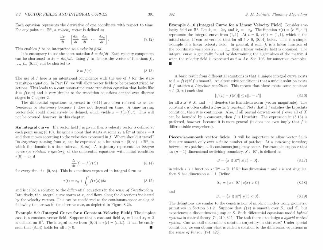
8.3. VECTOR FIELDS AND INTEGRAL CURVES 391
Each equation represents the derivative of one coordinate with respect to time.For any point x ∈ Rn, a velocity vector is defined as
dx
dt=
[
dx1dt
dx2dt· · · dxn
dt
]
. (8.12)
This enables f to be interpreted as a velocity field.It is customary to use the short notation x = dx/dt. Each velocity component
can be shortened to xi = dxi/dt. Using f to denote the vector of functions f1,. . ., fn, (8.11) can be shorted to
x = f(x). (8.13)
The use of f here is an intentional coincidence with the use of f for the statetransition equation. In Part IV, we will allow vector fields to be parameterized byactions. This leads to a continuous-time state transition equation that looks likex = f(x, u) and is very similar to the transition equations defined over discretestages in Chapter 2.
The differential equations expressed in (8.11) are often referred to as au-tonomous or stationary because f does not depend on time. A time-varyingvector field could alternatively be defined, which yields x = f(x(t), t). This willnot be covered, however, in this chapter.
An integral curve If a vector field f is given, then a velocity vector is defined ateach point using (8.10). Imagine a point that starts at some x0 ∈ Rn at time t = 0and then moves according to the velocities expressed in f . Where should it travel?Its trajectory starting from x0 can be expressed as a function τ : [0,∞)→ Rn, inwhich the domain is a time interval, [0,∞). A trajectory represents an integralcurve (or solution trajectory) of the differential equations with initial conditionτ(0) = x0 if
dτ
dt(t) = f(τ(t)) (8.14)
for every time t ∈ [0,∞). This is sometimes expressed in integral form as
τ(t) = x0 +
∫ t
0
f(τ(s))ds (8.15)
and is called a solution to the differential equations in the sense of Caratheodory.Intuitively, the integral curve starts at x0 and flows along the directions indicatedby the velocity vectors. This can be considered as the continuous-space analog offollowing the arrows in the discrete case, as depicted in Figure 8.2b.
Example 8.9 (Integral Curve for a Constant Velocity Field) The simplestcase is a constant vector field. Suppose that a constant field x1 = 1 and x2 = 2is defined on R2. The integral curve from (0, 0) is τ(t) = (t, 2t). It can be easilyseen that (8.14) holds for all t ≥ 0.
392 S. M. LaValle: Planning Algorithms
Example 8.10 (Integral Curve for a Linear Velocity Field) Consider a ve-locity field on R2. Let x1 = −2x1 and x2 = −x2. The function τ(t) = (e−2t, e−t)represents the integral curve from (1, 1). At t = 0, τ(0) = (1, 1), which is theinitial state. If can be verified that for all t > 0, (8.14) holds. This is a simpleexample of a linear velocity field. In general, if each fi is a linear function ofthe coordinate variables x1, . . ., xn, then a linear velocity field is obtained. Theintegral curve is generally found by determining the eigenvalues of the matrix Awhen the velocity field is expressed as x = Ax. See [106] for numerous examples.
A basic result from differential equations is that a unique integral curve existsto x = f(x) if f is smooth. An alternative condition is that a unique solution existsif f satisfies a Lipschitz condition. This means that there exists some constantc ∈ (0,∞) such that
‖f(x)− f(x′)‖ ≤ c‖x− x′‖ (8.16)
for all x, x′ ∈ X, and ‖ · ‖ denotes the Euclidean norm (vector magnitude). Theconstant c is often called a Lipschitz constant. Note that if f satisfies the Lipschitzcondition, then it is continuous. Also, if all partial derivatives of f over all of Xcan be bounded by a constant, then f is Lipschitz. The expression in (8.16) ispreferred, however, because it is more general (it does not even imply that f isdifferentiable everywhere).
Piecewise-smooth vector fields It will be important to allow vector fieldsthat are smooth only over a finite number of patches. At a switching boundarybetween two patches, a discontinuous jump may occur. For example, suppose thatan (n− 1)-dimensional switching boundary, S ⊂ Rn, is defined as
S = x ∈ Rn| s(x) = 0, (8.17)
in which s is a function s : Rn → R. If Rn has dimension n and s is not singular,then S has dimension n− 1. Define
S+ = x ∈ Rn| s(x) > 0 (8.18)
andS− = x ∈ Rn| s(x) < 0. (8.19)
The definitions are similar to the construction of implicit models using geometricprimitives in Section 3.1.2. Suppose that f(x) is smooth over S+ and S− butexperiences a discontinuous jump at S. Such differential equations model hybridsystems in control theory [74, 210, 325]. The task there is to design a hybrid controlsystem. Can we still determine a solution trajectory in this case? Under specialconditions, we can obtain what is called a solution to the differential equations inthe sense of Filipov [174, 426].

8.3. VECTOR FIELDS AND INTEGRAL CURVES 393
Let B(x, δ) denote an open ball of radius δ centered at x. Let f(B(x, δ))denote the set
f(B(x, δ)) = x′ ∈ X | ∃x′′ ∈ B(x, δ) for which x′ = f(x′′). (8.20)
Let X0 denote any subset of Rn that has measure zero (i.e., µ(X0) = 0). Lethull(A) denote the convex hull of a set, A, of points in Rn. A path τ : [0, tf ]→ Rn
is called a solution in the sense of Filipov if for almost all t ∈ [0, tf ],
dτ
dt(t) ∈
⋂
δ>0
⋂
X0
hull(f(B(τ(t), δ) \X0))
, (8.21)
in which the intersections are taken over all possible δ > 0 and sets, X0, of measurezero. The expression (8.21) is actually called a differential inclusion [39] becausea set of choices is possible for x. The “for almost all” requirement means that thecondition can even fail to hold on a set of measure zero in [0, tf ]. Intuitively, itsays that almost all of the velocity vectors produced by τ must point “between”the velocity vectors given by f in the vicinity of τ(x(t)). The “between” partcomes from using the convex hull. Filipov’s sense of solution is an incrediblegeneralization of the solution concept in the sense of Caratheodory. In that case,every velocity vector produced by τ must agree with f(x(t)), as given in (8.14).The condition in (8.21) allows all sorts of sloppiness to appear in the solution,even permitting f to be discontinuous.
Many bizarre vector fields can yield solutions in the sense of Filipov. Theswitching boundary model is relatively simple among those permitted by Fil-ipov’s condition. Figure 8.7 shows various cases that can occur at the switchingboundary S. For the case of consistent flow, solutions occur as you may intu-itively expect. Filipov’s condition, (8.21), requires that at S the velocity vectorof τ points between vectors before and after crossing S (for example, it can pointdown, which is the average of the two directions). The magnitude must also bebetween the two magnitudes. For the inward flow case, the integral curve movesalong S, assuming the vectors inside of S point in the same direction (withinthe convex hull) as the vectors on either side of the boundary. In applicationsthat involve physical systems, this may lead to oscillations around S. This canbe alleviated by regularization, which thickens the boundary [426] (the subject ofsliding-mode control addresses this issue [159]). The outward flow case can lead tononuniqueness if the initial state lies in S. However, trajectories that start outsideof S will not cross S, and there will be no such troubles. If the flow is tangenton both sides of a boundary, then other forms of nonuniqueness may occur. Thetangent-flow case will be avoided in this chapter.
8.3.2 Smooth Manifolds
The manifold definition given in Section 4.1.2 is often called a topological manifold.A manifold defined in this way does not necessarily have enough axioms to ensure
394 S. M. LaValle: Planning Algorithms
Consistent Flow Inward Flow
Outward flow Tangent flow
Figure 8.7: Different kinds of flows around a switching boundary.
that calculus operations, such as differentiation and integration, can be performed.We would like to talk about velocities on the configuration space C or in general fora continuous state space X. As seen in Chapter 4, the configuration space couldbe a manifold such as RP3. Therefore, we need to define some more qualities thata manifold should possess to enable calculus. This leads to the notion of a smoothmanifold.
Assume that M is a topological manifold, as defined in Section 4.1.2. Forexample, M could represent SO(3), the set of all rotation matrices for R3. Asimpler example that will be helpful to keep in mind is M = S2, which is a spherein R3. We want to extend the concepts of Section 8.3.1 from Rn to manifolds.One of the first definitions will be the tangent space Tp(M) at a point p ∈ M .As you might imagine intuitively, the tangent vectors are tangent to a surface,as shown in Figure 8.8. These will indicate possible velocities with which we canmove along the manifold from p. This is more difficult to define for a manifoldthan for Rn because it is easy to express any point in Rn using n coordinates, andall local coordinate frames for the tangent spaces at every p ∈ Rn are perfectlyaligned with each other. For a manifold such as S2, we must define tangent spacesin a way that is not sensitive to coordinates and handles the fact that the tangentplane rotates as we move around on S2.
First think carefully about what it means to assign coordinates to a manifold.Suppose M has dimension n and is embedded in Rm. For M = SO(3), n = 3 andm = 9. For M = S2, n = 2 and m = 3. The number of coordinates should be n,

8.3. VECTOR FIELDS AND INTEGRAL CURVES 395
M
Tp(M)
Figure 8.8: Intuitively, the tangent space is a linear approximation to the manifoldin a neighborhood around p.
the dimension of M ; however, manifolds embedded in Rm are often expressed asa subset of Rm for which some equality constraints must be obeyed. We wouldlike to express some part of M in terms of coordinates in Rn.
Coordinates and parameterizations For any open set U ⊆M and functionφ : U → Rn such that φ is a homeomorphism onto a subset of Rn, the pair (U, φ)is called a coordinate neighborhood (or chart in some literature). The values φ(p)for some p ∈ U are called the coordinates of p.
Example 8.11 (Coordinate Neighborhoods on S1) A simple example can beobtained for the circle M = S1. Suppose M is expressed as the unit circle embed-ded in R2 (the set of solutions to x2+y2 = 1). Let (x, y) denote a point in R2. LetU be the subset of S1 for which x > 0. A coordinate function φ : U → (−π/2, π/2),can be defined as φ(x, y) = tan−1(y/x).
LetW = φ(U) (the range of φ) for some coordinate neighborhood (U, φ). SinceU and W are homeomorphic via φ, the inverse function φ−1 can also be defined.It turns out that the inverse is the familiar idea of a parameterization. ContinuingExample 8.11, φ−1 yields the mapping θ 7→ (cos θ, sin θ), which is the familiarparameterization of the circle but restricted to θ ∈ (−π/2, π/2).
To make differentiation work at a point p ∈M , it will be important to have acoordinate neighborhood defined over an open subset of M that contains p. Thisis mainly because defining derivatives of a function at a point requires that anopen set exists around the point. If the coordinates appear to have no boundary,then this will be possible. It is unfortunately not possible to cover all ofM with asingle coordinate neighborhood, unless M = Rn (or M is at least homeomorphicto Rn). We must therefore define multiple neighborhoods for which the domains
396 S. M. LaValle: Planning Algorithms
Rn
Rn
U V
Mφ ψ
ψ φ−1
Figure 8.9: An illustration of a change of coordinates.
cover all of M . Since every domain is an open set, some of these domains mustoverlap. What happens in this case? We may have two or more alternativecoordinates for the same point. Moving from one set of coordinates to another isthe familiar operation used in calculus called a change of coordinates. This willnow be formalized.
Suppose that (U, φ) and (V, ψ) are coordinate neighborhoods on some manifoldM , and U ∩ V 6= ∅. Figure 8.9 indicates how to change coordinates from φ to ψ.This change of coordinates is expressed using function composition as ψ φ−1 :Rn → Rn (φ−1 maps from Rn into M , and ψ maps from a subset of M to Rn).
Example 8.12 (Change of Coordinates) Consider changing from Euler an-gles to quaternions for M = SO(3). Since SO(3) is a 3D manifold, n = 3. Thismeans that any coordinate neighborhood must map a point in SO(3) to a point inR3. We can construct a coordinate function φ : SO(3)→ R3 by computing Eulerangles from a given rotation matrix. The functions are actually defined in (3.47),(3.48), and (3.49). To make this a coordinate neighborhood, an open subset U ofM must be specified.
We can construct another coordinate function ψ : SO(3) → R3 by usingquaternions. This may appear to be a problem because quaternions have fourcomponents; however, the fourth component can be determined from the otherthree. Using (4.24) to (4.26), the a, b, and c coordinates can be determined.
Now suppose that we would like to change from Euler angles to quaternionsin the overlap region U ∩ V , in which V is an open set on which the coordinateneighborhood for quaternions is defined. The task is to construct a change ofcoordinates, ψ φ−1. We first have to invert φ over U . This means that weinstead need a parameterization of M in terms of Euler angles. This is givenby (3.42), which yields a rotation matrix, φ−1(α, β, γ) ∈ SO(3) for α, β, and γ.Once this matrix is determined, then ψ can be applied to it to determine thequaternion parameters, a, b, and c. This means that we have constructed threereal-valued functions, f1, f2, and f3, which yield a = f1(α, β, γ), b = f2(α, β, γ),and c = f3(α, β, γ). Together, these define ψ φ−1.
8.3. VECTOR FIELDS AND INTEGRAL CURVES 397
There are several reasons for performing coordinate changes in various con-texts. Example 8.12 is motivated by a change that frequently occurs in motionplanning. Imagine, for example, that a graphics package displays objects usingquaternions, but a collision-detection algorithm uses Euler angles. It may be nec-essary in such cases to frequently change coordinates. From studies of calculus,you may recall changing coordinates to simplify an integral. In the definition of asmooth manifold, another motivation arises. Since coordinate neighborhoods arebased on homeomorphisms of open sets, several may be required just to cover allofM . For example, even if we decide to use quaternions for SO(3), several coordi-nate neighborhoods that map to quaternions may be needed. On the intersectionsof their domains, a change of coordinates is necessary.
Now we are ready to define a smooth manifold. Changes of coordinates willappear in the manifold definition, and they must satisfy a smoothness condition.A smooth structure5 on a (topological) manifold M is a family6 U = Uα, φα ofcoordinate neighborhoods such that:
1. The union of all Uα contains M . Thus, it is possible to obtain coordinatesin Rn for any point in M .
2. For any (U, φ) and (V, ψ) in U , if U∩V 6= ∅, then the changes of coordinates,ψ φ−1 and φ ψ−1, are smooth functions on U ∩ V . The changes ofcoordinates must produce diffeomorphisms on the intersections. In this case,the coordinate neighborhoods are called compatible.
3. The family U is maximal in the sense that if some (U, φ) is compatible withevery coordinate neighborhood in U , then (U, φ) must be included in U .
A well-known theorem (see [73], p. 54) states that if a set of compatible neighbor-hoods covers all ofM , then a unique smooth structure exists that contains them.7
This means that a differential structure can often be specified by a small numberof neighborhoods, and the remaining ones are implied.
A manifold, as defined in Section 4.1.2, together with a smooth structure iscalled a smooth manifold.8
Example 8.13 (Rn as a Smooth Manifold) We should expect that the con-cepts presented so far apply to Rn, which is the most straightforward family ofmanifolds. A single coordinate neighborhood Rn → Rn can be used, which is theidentity map. For all integers n ∈ 1, 2, 3 and n > 4, this is the only possiblesmooth structure on Rn. It is truly amazing that for R4, there are uncountably
5Alternative names are differentiable structure and C∞ structure.6In literature in which the coordinate neighborhoods are called charts, this family is called
an atlas.7This is under the assumption that M is Hausdorff and has a countable basis of open sets,
which applies to the manifolds considered here.8Alternative names are differentiable manifold and C∞ manifold.
398 S. M. LaValle: Planning Algorithms
many incompatible smooth structures, called exotic R4 [155]. There is no need toworry, however; just use the one given by the identity map for R4.
Example 8.14 (Sn as a Smooth Manifold) One way to define Sn as a smoothmanifold uses 2(n+1) coordinate neighborhoods and results in simple expressions.Let Sn be defined as
Sn = (x1, . . . , xn+1) ∈ Rn+1| x21 + · · ·+ x2n+1 = 1. (8.22)
The domain of each coordinate neighborhood is defined as follows. For each ifrom 1 to n+ 1, there are two neighborhoods:
U+i = (x1, . . . , xn+1) ∈ Rn+1| xi > 0 (8.23)
andU−i = (x1, . . . , xn+1) ∈ Rn+1| xi < 0. (8.24)
Each neighborhood is an open set that covers half of Sn but misses the great circleat xi = 0. The coordinate functions can be defined by projection down to the(n− 1)-dimensional hyperplane that contains the great circle. For each i,
φ+i (x1, . . . , xn+1) = (x1, . . . , xi−1, xi+1, . . . , xn) (8.25)
over U+i . Each φ
−i is defined the same way, but over U−
i . Each coordinate functionis a homeomorphism from an open subset of Sn to an open subset of Rn, asrequired. On the subsets in which the neighborhoods overlap, the changes ofcoordinate functions are smooth. For example, consider changing from φ+
i to φ−j
for some i 6= j. The change of coordinates is a function φ−j (φ+
i )−1. The inverse
of φ+i is expressed as
(φ+i )
−1(x1, . . . , xi−1, xi+1, . . . , xn) =
(x1, . . . , xi−1, 1−√
1− x21 − · · · − x2i−1 − x2i+1 − · · · − x2n, xi+1, . . . , xn+1).(8.26)
When composed with φ−j , the jth coordinate is dropped. This yields
φ−k (φ+
i )−1(x1, . . . , xi−1, xi+1, . . . , xn) =
(x1, . . . , xi−1, 1−√
1− x21 − · · · − x2i−1 − x2i+1 − · · · − x2n,xi+1, . . . , xj−1, xj+1, . . . , xn),
(8.27)
which is a smooth function over the domain U+i . Try visualizing the changes of
coordinates for the circle S1 and sphere S2.The smooth structure can alternatively be defined using only two coordinate
neighborhoods by using stereographic projection. For S2, one coordinate functionmaps almost every point x ∈ S2 to R2 by drawing a ray from the north pole to

8.3. VECTOR FIELDS AND INTEGRAL CURVES 399
x and mapping to the point in the x3 = 0 plane that is crossed by the ray. Theonly excluded point is the north pole itself. A similar mapping can be constructedfrom the south pole.
Example 8.15 (RPn as a Smooth Manifold) This example is particularly im-portant because RP3 is the same manifold as SO(3), as established in Section 4.2.2.Recall from Section 4.1.2 that RPn is defined as the set of all lines in Rn+1 thatpass through the origin. This means that for any α ∈ R such that α 6= 0, andany x ∈ Rn+1, both x and αx are identified. In projective space, scale does notmatter.
A smooth structure can be specified by only n+ 1 coordinate neighborhoods.For each i from 1 to n+ 1, let
φi(x1, . . . , xn+1) = (x1/xi, . . . , xi−1/xi, xi+1/xi, . . . , xn/xi), (8.28)
over the open set of all points in Rn+1 for which xi 6= 0. The inverse coordinatefunction is given by
φ−1i (z1, . . . , zn) = (z1, . . . , zi−1, 1, zi, . . . , zn+1). (8.29)
It is not hard to verify that these simple transformations are smooth on overlap-ping neighborhoods.
A smooth structure over SO(3) can be derived as a special case because SO(3)is topologically equivalent to RP3. Suppose elements of SO(3) are expressed usingunit quaternions. Each (a, b, c, d) is considered as a point on S3. There are fourcoordinate neighborhoods. For example, one of them is
φb(a, b, c, d) = (a/b, c/b, d/b), (8.30)
which is defined over the subset of R4 for which b 6= 0. The inverse of φb(a, b, c, d)needs to be defined so that a point on SO(3) maps to a point in R4 that has unitmagnitude.
Tangent spaces on manifolds Now consider defining tangent spaces on man-ifolds. Intuitively, the tangent space Tp(M) at a point p on an n-dimensionalmanifold M is an n-dimensional hyperplane in Rm that best approximates Maround p, when the hyperplane origin is translated to p. This is depicted in Fig-ure 8.8. The notion of a tangent was actually used in Section 7.4.1 to describelocal motions for motion planning of closed kinematic chains (see Figure 7.22).
To define a tangent space on a manifold, we first consider a more complicateddefinition of the tangent space at a point in Rn, in comparison to what was given inSection 8.3.1. Suppose that M = R2, and consider taking directional derivatives
400 S. M. LaValle: Planning Algorithms
of a smooth function f : R2 → R at a point p ∈ R2. For some (unnormalized)direction vector, v ∈ R2, the directional derivative of f at p can be defined as
∇v(f)∣
∣
∣
p= v1
∂f
∂x1
∣
∣
∣
p+ v2
∂f
∂x2
∣
∣
∣
p. (8.31)
The directional derivative used here does not normalize the direction vector (con-trary to basic calculus). Hence, ∇v(f) = ∇(f) · v, in which “·” denotes the innerproduct or dot product, and∇(f) denotes the gradient of f . The set of all possibledirection vectors that can be used in this construction forms a two-dimensionalvector space that happens to be the tangent space Tp(R
2), as defined previously.This can be generalized to n dimensions to obtain
∇v(f)∣
∣
∣
p=
n∑
i=1
vi∂f
∂xi
∣
∣
∣
p, (8.32)
for which all possible direction vectors represent the tangent space Tp(Rn). The
set of all directions can be interpreted for our purposes as the set of possiblevelocity vectors.
Now consider taking (unnormalized) directional derivatives of a smooth func-tion, f :M → R, on a manifold. For an n-dimensional manifold, the tangent spaceTp(M) at a point p ∈ M can be considered once again as the set of all unnor-malized directions. These directions must intuitively be tangent to the manifold,as depicted in Figure 8.8. There exists a clever way to define them without evenreferring to specific coordinate neighborhoods. This leads to a definition of Tp(M)that is intrinsic to the manifold.
At this point, you may accept that Tp(M) is an n-dimensional vector spacethat is affixed to M at p and oriented as shown in Figure 8.8. For the sake ofcompleteness, however, a technical definition of Tp(M) from differential geometrywill be given; more details appear in [73, 437]. The construction is based oncharacterizing the set of all possible directional derivative operators. Let C∞(p)denote the set of all smooth functions that have domains that include p. Nowmake the following identification. Any two functions f, g ∈ C∞(p) are definedto be equivalent if there exists an open set U ⊂ M such that for any p ∈ U ,f(p) = g(p). There is no need to distinguish equivalent functions because theirderivatives must be the same at p. Let C∞(p) denote C∞ under this identification.A directional derivative operator at p can be considered as a function that mapsfrom C∞(p) to R for some direction. In the case of Rn, the operator appears as∇v for each direction v. Think about the set of all directional derivative operatorsthat can be made. Each one must assign a real value to every function in C∞(p),and it must obey two axioms from calculus regarding directional derivatives. Let∇v denote a directional derivative operator at some p ∈ M (be careful, however,because here v is not explicitly represented since there are no coordinates). Thedirectional derivative operator must satisfy two axioms:
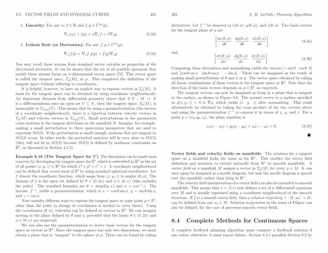
8.3. VECTOR FIELDS AND INTEGRAL CURVES 401
1. Linearity: For any α, β ∈ R and f, g ∈ C∞(p),
∇v(αf + βg) = α∇vf + β∇vg. (8.33)
2. Leibniz Rule (or Derivation): For any f, g ∈ C∞(p),
∇v(fg) = ∇vf g(p) + f(p)∇vg. (8.34)
You may recall these axioms from standard vector calculus as properties of thedirectional derivative. It can be shown that the set of all possible operators thatsatisfy these axioms forms an n-dimensional vector space [73]. This vector spaceis called the tangent space, Tp(M), at p. This completes the definition of thetangent space without referring to coordinates.
It is helpful, however, to have an explicit way to express vectors in Tp(M). Abasis for the tangent space can be obtained by using coordinate neighborhoods.An important theorem from differential geometry states that if F : M → Nis a diffeomorphism onto an open set U ⊂ N , then the tangent space, Tp(M), isisomorphic to TF (p)(N). This means that by using a parameterization (the inverseof a coordinate neighborhood), there is a bijection between velocity vectors inTp(M) and velocity vectors in TF (p)(N). Small perturbations in the parameterscause motions in the tangent directions on the manifold N . Imagine, for example,making a small perturbation to three quaternion parameters that are used torepresent SO(3). If the perturbation is small enough, motions that are tangent toSO(3) occur. In other words, the perturbed matrices will lie very close to SO(3)(they will not lie in SO(3) because SO(3) is defined by nonlinear constraints onR9, as discussed in Section 4.1.2).
Example 8.16 (The Tangent Space for S2) The discussion can be made moreconcrete by developing the tangent space for S2, which is embedded in R3 as the setof all points (x, y, z) ∈ R3 for which x2 + y2 + z2 = 1. A coordinate neighborhoodcan be defined that covers most of S2 by using standard spherical coordinates. Letf denote the coordinate function, which maps from (x, y, z) to angles (θ, φ). Thedomain of f is the open set defined by θ ∈ (0, 2π) and φ ∈ (0, π) (this excludesthe poles). The standard formulas are θ = atan2(y, x) and φ = cos−1 z. Theinverse, f−1, yields a parameterization, which is x = cos θ sinφ, y = sin θ sinφ,and z = cosφ.
Now consider different ways to express the tangent space at some point p ∈ S2,other than the poles (a change of coordinates is needed to cover these). Usingthe coordinates (θ, φ), velocities can be defined as vectors in R2. We can imaginemoving in the plane defined by θ and φ, provided that the limits θ ∈ (0, 2π) andφ ∈ (0, π) are respected.
We can also use the parameterization to derive basis vectors for the tangentspace as vectors in R3. Since the tangent space has only two dimensions, we mustobtain a plane that is “tangent” to the sphere at p. These can be found by taking
402 S. M. LaValle: Planning Algorithms
derivatives. Let f−1 be denoted as x(θ, φ), y(θ, φ), and z(θ, φ). Two basis vectorsfor the tangent plane at p are
[
dx(θ, φ)
dθ
dy(θ, φ)
dθ
dz(θ, φ)
dθ
]
(8.35)
and[
dx(θ, φ)
dφ
dy(θ, φ)
dφ
dz(θ, φ)
dφ
]
. (8.36)
Computing these derivatives and normalizing yields the vectors [− sin θ cos θ 0]and [cos θ cosφ sin θ cosφ − sinφ]. These can be imagined as the result ofmaking small perturbations of θ and φ at p. The vector space obtained by takingall linear combinations of these vectors is the tangent space at R2. Note that thedirection of the basis vectors depends on p ∈ S2, as expected.
The tangent vectors can now be imagined as lying in a plane that is tangentto the surface, as shown in Figure 8.8. The normal vector to a surface specifiedas g(x, y, z) = 0 is ∇g, which yields [x y z] after normalizing. This couldalternatively be obtained by taking the cross product of the two vectors aboveand using the parameterization f−1 to express it in terms of x, y, and z. For apoint p = (x0, y0, z0), the plane equation is
x0(x− x0) + y0(y − y0) + z0(z − z0) = 0. (8.37)
Vector fields and velocity fields on manifolds The notation for a tangentspace on a manifold looks the same as for Rn. This enables the vector fielddefinition and notation to extend naturally from Rn to smooth manifolds. Avector field on a manifold M assigns a vector in Tp(M) for every p ∈ M . It canonce again be imagined as a needle diagram, but now the needle diagram is spreadover the manifold, rather than lying in Rn.
The velocity field interpretation of a vector field can also be extended to smoothmanifolds. This means that x = f(x) now defines a set of n differential equationsover M and is usually expressed using a coordinate neighborhood of the smoothstructure. If f is a smooth vector field, then a solution trajectory, τ : [0,∞)→M ,can be defined from any x0 ∈M . Solution trajectories in the sense of Filipov canalso be defined, for the case of piecewise-smooth vector fields.
8.4 Complete Methods for Continuous Spaces
A complete feedback planning algorithm must compute a feedback solution ifone exists; otherwise, it must report failure. Section 8.4.1 parallels Section 8.2 by

8.4. COMPLETE METHODS FOR CONTINUOUS SPACES 403
defining feedback plans and navigation functions for the case of a continuous statespace. Section 8.4.2 indicates how to define a feasible feedback plan from a cellcomplex that was computed using cell decomposition techniques. Section 8.4.3presents a combinatorial approach to computing an optimal navigation functionand corresponding feedback plan in R2. Sections 8.4.2 and 8.4.3 allow the feedbackplan to be a discontinuous vector field. In many applications, especially those inwhich dynamics dominate, some conditions need to be enforced on the naviga-tion functions and their resulting vector fields. Section 8.4.4 therefore considersconstraints on the allowable vector fields and navigation functions. This coverageincludes navigation functions in the sense of Rimon-Koditschek [416], from whichthe term navigation function was introduced.
8.4.1 Feedback Motion Planning Definitions
Using the concepts from Section 8.3, we are now ready to define feedback mo-tion planning over configuration spaces or other continuous state spaces. RecallFormulation 4.1, which defined the basic motion planning problem in terms ofconfiguration space. The differences in the current setting are that there is noinitial condition, and the requirement of a solution path is replaced by a solu-tion vector field. The formulation here can be considered as a continuous-timeadaptation to Formulation 8.1.
Formulation 8.2 (Feedback Motion Planning)
1. A state space, X, which is a smooth manifold. The state space will mostoften be Cfree, as defined in Section 4.3.1.9
2. For each state, x ∈ X, an action space, U(x) = Tx(X). The zero velocity,0 ∈ Tx(X), is designated as the termination action, uT . Using this model,the robot is capable of selecting its velocity at any state.10
3. An unbounded time interval, T = [0,∞).
4. A state transition (differential) equation,
x = u, (8.38)
which is expressed using a coordinate neighborhood and yields the velocity,x, directly assigned by the action u. The velocity produced by uT is 0 ∈Tx(X) (which means “stop”).
9Note that X already excludes the obstacle region. For some problems in Part IV, the statespace will be X = C, which includes the obstacle region.
10This allows discontinuous changes in velocity, which is unrealistic in many applications.Additional constraints, such as imposing acceleration bounds, will also be discussed. For acomplete treatment of differential constraints, see Part IV.
404 S. M. LaValle: Planning Algorithms
5. A goal set, XG ⊂ X.
A feedback plan, π, for Formulation 8.2 is defined as a function π, which pro-duces an action u ∈ U(x) for each x ∈ X. A feedback plan can equivalently beconsidered as a vector field on X because each u ∈ U(x) specifies a velocity vector(uT specifies zero velocity). Since the initial state is not fixed, it becomes slightlymore complicated to define what it means for a plan to be a solution to the prob-lem. Let Xr ⊂ X denote the set of all states from which XG is reachable. Moreprecisely, a state xI belongs to Xr if and only if a continuous path τ : [0, 1]→ Xexists for which τ(0) = xI and τ(1) = xG for some xG ∈ XG. This means that asolution path exists from xI for the “open-loop” motion planning problem, whichwas considered in Chapter 4.
Solution concepts
A feedback plan, π, is called a solution to the problem in Formulation 8.2 if fromall xI ∈ Xr, the integral curves of π (considered as a vector field) arrive in XG,at which point the termination action is applied. Some words of caution must begiven about what it means to “arrive” in XG. Notions of stability from controltheory [271, 426] are useful for distinguishing different cases; see Section 15.1. IfXG is a small ball centered on xG, then the ball will be reached after finite timeusing the inward vector field shown in Figure 8.5b. Now suppose that XG is asingle point, xG. The inward vector field produces velocities that bring the statecloser and closer to the origin, but when is it actually reached? It turns out thatconvergence to the origin in this case is only asymptotic; the origin is reached in thelimit as the time approaches infinity. Such stability often arises in control theoryfrom smooth vector fields. We may allow such asymptotic convergence to the goal(if the vector field is smooth and the goal is a point, then this is unavoidable).If any integral curves result in only asymptotic convergence to the goal, then asolution plan is called an asymptotic solution plan. Note that in general it maybe impossible to require that π is a smooth (or even continuous) nonzero vectorfield. For example, due to the hairy ball theorem [419], it is known that no suchvector field exists for Sn for any even integer n. Therefore, the strongest possiblerequirement is that π is smooth except on a set of measure zero; see Section 8.4.4.We may also allow solutions π for which almost all integral curves arrive in XG.
However, it will be assumed by default in this chapter that a solution planconverges to xG in finite time. For example, if the inward field is normalized toproduce unit speed everywhere except the origin, then the origin will be reached infinite time. A constraint can be placed on the set of allowable vector fields withoutaffecting the existence of a solution plan. As in the basic motion planning problem,the speed along the path is not important. Let a normalized vector field be anyvector field for which either ‖f(x)‖ = 1 or f(x) = 0, for all x ∈ X. This meansthat all velocity vectors are either unit vectors or the zero vector, and the speed isno longer a factor. A normalized vector field provides either a direction of motion

8.4. COMPLETE METHODS FOR CONTINUOUS SPACES 405
or no motion. Note that any vector field f can be converted into a normalizedvector field by dividing the velocity vector f(x) by its magnitude (unless themagnitude is zero), for each x ∈ X.
In many cases, unit speed does not necessarily imply a constant speed in sometrue physical sense. For example, if the robot is a floating rigid body, there aremany ways to parameterize position and orientation. The speed of the body issensitive to this parameterization. Therefore, other constraints may be preferableinstead of ‖f(x)‖ = 1; however, it is important to keep in mind that the constraintis imposed so that f(x) provides a direction at x. The particular magnitude isassumed unimportant.
So far, consideration has been given only to a feasible feedback motion plan-ning problem. An optimal feedback motion planning problem can be defined byintroducing a cost functional. Let xt denote the function xt : [0, t] → X, whichis called the state trajectory (or state history). This is a continuous-time ver-sion of the state history, which was defined previously for problems that havediscrete stages. Similarly, let ut denote the action trajectory (or action history),ut : [0, t]→ U . Let L denote a cost functional, which may be applied from any xIto yield
L(xtF , utF ) =
∫ tF
0
l(x(t), u(t))dt+ lF (x(tF )), (8.39)
in which tF is the time at which the termination action is applied. The terml(x(t), u(t)) can alternatively be expressed as l(x(t), x(t)) by using the state tran-sition equation (8.38). A normalized vector field that optimizes (8.39) from allinitial states that can reach the goal is considered as an optimal feedback motionplan.
Note that the state trajectory can be determined from an action history andinitial state. In fact, we could have used action trajectories to define a solutionpath to the motion planning problem of Chapter 4. Instead, a solution was definedthere as a path τ : [0, 1] → Cfree to avoid having to introduce velocity fields onsmooth manifolds. That was the only place in the book in which the actionspace seemed to disappear, and now you can see that it was only hiding to avoidinessential notation.
Navigation functions
As in Section 8.2.2, potential functions can be used to represent feedback plans,assuming that a local operator is developed that works for continuous state spaces.In the discrete case, the local operator selects an action that reduces the poten-tial value. In the continuous case, the local operator must convert the potentialfunction into a vector field. In other words, a velocity vector must be defined ateach state. By default, it will be assumed here that the vector fields derived fromthe navigation function are not necessarily normalized.
Assume that π(x) = uT is defined for all x ∈ XG, regardless of the potentialfunction. Suppose that a potential function φ : X → R has been defined for which
406 S. M. LaValle: Planning Algorithms
the gradient
∇φ =
[
∂φ
∂x1
∂φ
∂x2· · · ∂φ
∂xn
]
(8.40)
exists over all of X \ XG. The corresponding feedback plan can then be definedas π(x) = −∇φ|x. This defines the local operator, which means that the velocityis taken in the direction of the steepest descent of φ. The idea of using potentialfunctions in this way was proposed for robotics by Khatib [273, 274] and can beconsidered as a form of gradient descent, which is a general optimization technique.
It is also possible to work with potential functions for which the gradient doesnot exist everywhere. In these cases, a continuous-space version of (8.4) can bedefined for a small, fixed ∆t as
u∗ = argminu∈U(x)
φ(x′)
, (8.41)
in which x′ is the state obtained by integrating velocity u from x for time ∆t.One problem is that ∆t should be chosen to use the smallest possible neighbor-hood around φ. It is best to allow only potential functions for which ∆t can bemade arbitrarily small at every x without affecting the decision in (8.41). To beprecise, this means that an infinite sequence of u∗ values can be determined froma sequence of ∆t values that converges to 0. A potential function should thenbe chosen to ensure after some point in the sequence, u∗, exists and the same u∗
can be chosen to satisfy (8.41) as ∆t approaches 0. A special case of this is if thegradient of φ exists; the infinite sequence in this case converges to the negativegradient.
A potential function, φ, is called a navigation function if the vector field thatis derived from it is a solution plan. The optimal cost-to-go serves as an optimalnavigation function. If multiple vector fields can be derived from the same φ,then every possible derived vector field must yield a solution feedback plan. Ifdesigned appropriately, the potential function can be viewed as a kind of “skislope” that guides the state to XG. If there are extra local minima that causethe state to become trapped, then XG will not be reached. To be a navigationfunction, such local minima outside of XG are not allowed. Furthermore, theremay be additional requirements to ensure that the derived vector field satisfiesadditional constraints, such as bounded acceleration.
Example 8.17 (Quadratic Potential Function) As a simple example, sup-pose X = R2, there are no obstacles, and qgoal = (0, 0). A quadratic functionφ(x, y) = 1
2x21 +
12x22 serves as a good potential function to guide the state to the
goal. The feedback motion strategy is defined as f = −∇φ = [−x1 − x2], whichis the inward vector field shown in Figure 8.5b.
If the goal is instead at some (x′1, x′2) ∈ R2, then a potential function that
guides the state to the goal is φ(x1, x2) = (x1 − x′1)2 + (x2 − x′2)2.

8.4. COMPLETE METHODS FOR CONTINUOUS SPACES 407
Suppose the state space represents a configuration space that contains pointobstacles. The previous function φ can be considered as an attractive potentialbecause the configuration is attracted to the goal. One can also construct a repul-sive potential that repels the configuration from the obstacles to avoid collision.Let φa denote the attractive component and φr denote a repulsive potential that issummed over all obstacle points. A potential function of the form φ = φa+φr canbe defined to combine both effects. The robot should be guided to the goal whileavoiding obstacles. The problem is that it is difficult in general to ensure thatthe potential function will not contain multiple local minima. The configurationcould become trapped at a local minimum that is not in the goal region. Thiswas an issue with the planner from Section 5.4.3.
8.4.2 Vector Fields Over Cell Complexes
This section describes how to construct a piecewise-smooth vector field over acell complex. Only normalized vector fields will be considered. It is assumedthat each cell in the complex has a simple shape over which it is easy to define apatch of the vector field. In many cases, the cell decomposition techniques thatwere introduced in Chapter 6 for motion planning can be applied to construct afeedback plan.
Suppose that an n-dimensional state space X has been decomposed into a cellcomplex, such as a simplicial complex or singular complex, as defined in Section6.3.1. Assume that the goal set is a single point, xG. Defining a feedback plan πover X requires placing a vector field on X for which all integral curves lead toxG (if xG is reachable). This is accomplished by defining a smooth vector field foreach n-cell. Each (n − 1)-cell is a switching boundary, as considered in Section8.3.1. This leads directly to solution trajectories in the sense of Filipov. If π isallowed to be discontinuous, then it is actually not important to specify values onany of the cells of dimension n− 1 or less.
A hierarchical approach is taken to the construction of π:
1. Define a discrete planning problem over the n-cells. The cell that containsxG is designated as the goal, and a discrete navigation function is definedover the cells.
2. Define a vector field over each n-cell. The field should cause all states inthe cell to flow into the next cell as prescribed by the discrete navigationfunction.
One additional consideration that is important in applications is to try to reducethe effect of the discontinuity across the boundary as much as possible. It maybe possible to eliminate the discontinuity, or even construct a smooth transitionbetween n-cells. This issue will not be considered here, but it is nevertheless quiteimportant [127, 334].
408 S. M. LaValle: Planning Algorithms
The approach will now be formalized. Suppose that a cell complex has beendefined over a continuous state space, X. Let X denote the set of n-cells, whichcan be interpreted as a finite state space. A discrete planning problem will bedefined over X. To avoid confusion with the original continuous problem, theprefix super will be applied to the discrete planning components. Each superstatex ∈ X corresponds to an n-cell. From each x, a superaction, u ∈ U(x) exists foreach neighboring n-cell (to be neighboring, the two cells must share an (n − 1)-dimensional boundary). Let the goal superstate xg be the n-cell that contains xG.Assume that the cost functional is defined for the discrete problem so that everyaction (other than uT ) produces a unit cost. Now the concepts from Section 8.2can be applied to the discrete problem. A discrete navigation function, φ : X → R,can be computed using Dijkstra’s algorithm (or another algorithm, particularly ifoptimality is not important). Using the discrete local operator from Section 8.2.2,this results in a discrete feedback plan, π : X → U .
Based on the discrete feedback plan, there are two kinds of n-cells. The firstis the goal cell, xg, for which a vector field needs to be defined so that all integralcurves lead to Xg in finite time.11 A termination action can be applied when xGis actually reached. The remaining n-cells are of the second kind. For each cellx, the boundary that is shared with the cell reached by applying u = π(x) iscalled the exit face. The vector field over the n-cell x must be defined so that allintegral curves lead to the exit face. When the exit face is reached, a transition willoccur into the next n-cell. If the n-cells are convex, then defining this transitionis straightforward (unless there are additional requirements on the field, such assmoothness at the boundary). For more complicated cells, one possibility is todefine a vector field that retracts all points onto a single curve in the cell.
A simple example of the approach is illustrated for the case of X = Cfree ⊂ R2,in which the boundary of Cfree is polygonal. This motion planning problem wasconsidered in Section 6.2, but without feedback. Suppose that a triangulation ofX has been computed, as described in Section 6.3.2. An example was shown inFigure 6.16. A discrete feedback plan is shown for a particular goal state in Figure8.10. Each 2-cell (triangle) is labeled with an arrow that points to the next cell.
For the cell that contains xG, a normalized version of the inward vector fieldshown in Figure 8.5b can be formed by dividing each nonzero vector by its magni-tude. It can then be translated to move its origin to xG. For each remaining 2-cell,a vector field must be constructed that flows into the appropriate neighboring cell.Figure 8.11 illustrates a simple way to achieve this. An outward vector field canbe made by negating the field shown in Figure 8.5b to obtain f = [x y]. Thisfield can be normalized and translated to move the origin to the triangle vertexthat is not incident to the exit edge. This is called the repulsive vertex in Figure8.11. This generates a vector field that pushes all points in the triangle to the extedge. If the fields are constructed in this way for each triangle, then the global
11This is possible in finite time, even if Xg is a single point, because the vector field is notcontinuous. Otherwise, only asymptotic convergence may be possible.
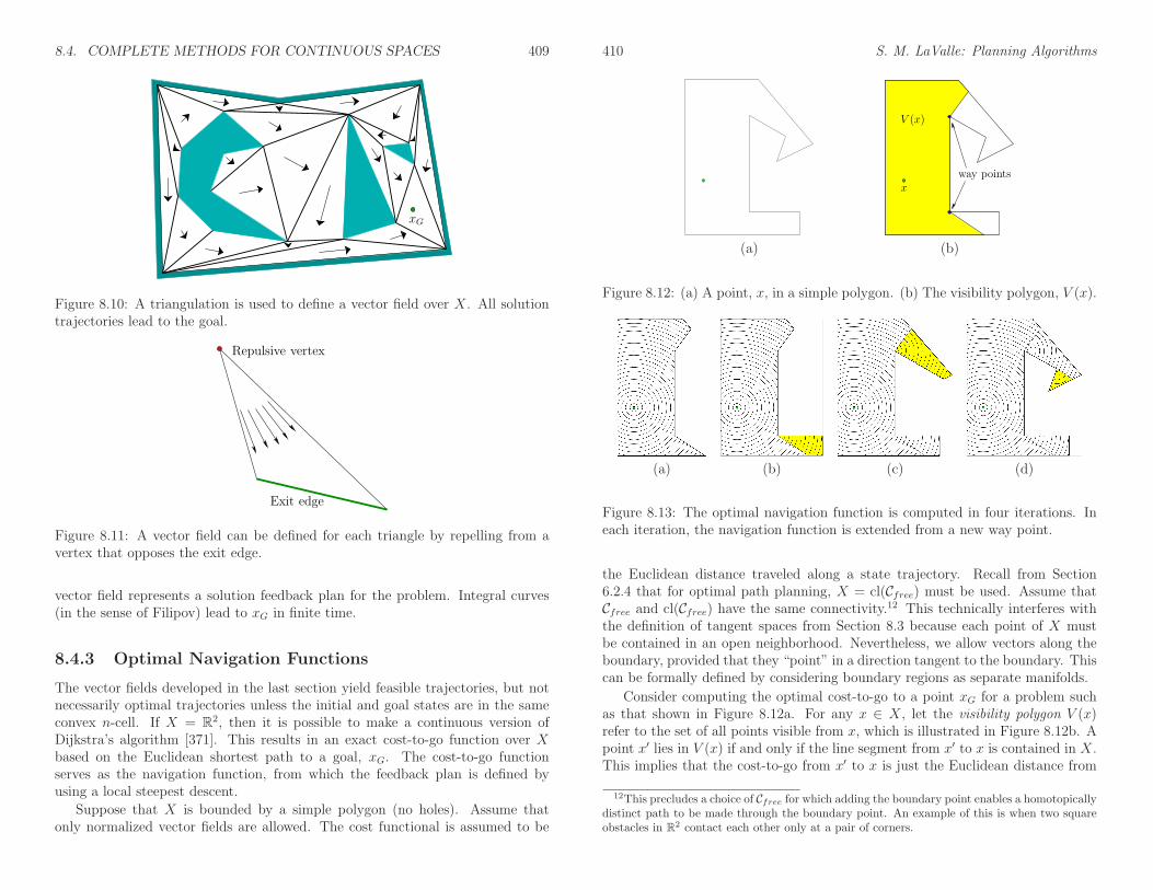
8.4. COMPLETE METHODS FOR CONTINUOUS SPACES 409
xG
Figure 8.10: A triangulation is used to define a vector field over X. All solutiontrajectories lead to the goal.
Repulsive vertex
Exit edge
Figure 8.11: A vector field can be defined for each triangle by repelling from avertex that opposes the exit edge.
vector field represents a solution feedback plan for the problem. Integral curves(in the sense of Filipov) lead to xG in finite time.
8.4.3 Optimal Navigation Functions
The vector fields developed in the last section yield feasible trajectories, but notnecessarily optimal trajectories unless the initial and goal states are in the sameconvex n-cell. If X = R2, then it is possible to make a continuous version ofDijkstra’s algorithm [371]. This results in an exact cost-to-go function over Xbased on the Euclidean shortest path to a goal, xG. The cost-to-go functionserves as the navigation function, from which the feedback plan is defined byusing a local steepest descent.
Suppose that X is bounded by a simple polygon (no holes). Assume thatonly normalized vector fields are allowed. The cost functional is assumed to be
410 S. M. LaValle: Planning Algorithms
V (x)
way pointsx
(a) (b)
Figure 8.12: (a) A point, x, in a simple polygon. (b) The visibility polygon, V (x).
(a) (b) (c) (d)
Figure 8.13: The optimal navigation function is computed in four iterations. Ineach iteration, the navigation function is extended from a new way point.
the Euclidean distance traveled along a state trajectory. Recall from Section6.2.4 that for optimal path planning, X = cl(Cfree) must be used. Assume thatCfree and cl(Cfree) have the same connectivity.12 This technically interferes withthe definition of tangent spaces from Section 8.3 because each point of X mustbe contained in an open neighborhood. Nevertheless, we allow vectors along theboundary, provided that they “point” in a direction tangent to the boundary. Thiscan be formally defined by considering boundary regions as separate manifolds.
Consider computing the optimal cost-to-go to a point xG for a problem suchas that shown in Figure 8.12a. For any x ∈ X, let the visibility polygon V (x)refer to the set of all points visible from x, which is illustrated in Figure 8.12b. Apoint x′ lies in V (x) if and only if the line segment from x′ to x is contained in X.This implies that the cost-to-go from x′ to x is just the Euclidean distance from
12This precludes a choice of Cfree for which adding the boundary point enables a homotopicallydistinct path to be made through the boundary point. An example of this is when two squareobstacles in R2 contact each other only at a pair of corners.

8.4. COMPLETE METHODS FOR CONTINUOUS SPACES 411
x′ to x. The optimal navigation function can therefore be immediately definedover V (xG) as
φ(x) = ‖x− xG‖. (8.42)
Level sets at regularly spaced values of this navigation function are shown inFigure 8.13a.
How do we compute the optimal cost-to-go values for the points in X \V (xG)?For the segments on the boundary of V (x) for any x ∈ X, some edges are containedin the boundary ofX, and others cross the interior ofX. For the example in Figure8.12b, there are two edges that cross the interior. For each segment that crossesthe interior, let the closer of the two vertices to x be referred to as a way point.Two way points are indicated in Figure 8.12b. The way points of V (xG) are placesthrough which some optimal paths must cross. Let W (x) for any x ∈ X denotethe set of way points of V (x).
A straightforward algorithm proceeds as follows. Let Zi denote the set ofpoints over which φ has been defined, in the ith iteration of the algorithm. In thefirst iteration, Z1 = V (xG), which is the case shown in Figure 8.13a. The waypoints of V (xG) are placed in a queue, Q. In each following iteration, a way pointx is removed from Q. Let Zi denote the domain over which φ is defined so far.The domain of φ is extended to include all new points visible from x. These newpoints are V (x) \ Zi. This yields Zi+1 = Zi ∪ V (x), the extended domain of φ.The values of φ(x′) for x′ ∈ Zi+1 \ Zi are defined by
φ(x′) = φ(x) + ‖x′ − x‖, (8.43)
in which x is the way point that was removed from Q (the optimal cost-to-govalue of x was already computed). The way points of V (x) that do not lie in Zi+1
are added to Q. Each of these will yield new portions of X that have not yet beenseen. The algorithm terminates when Q is empty, which implies that Zk = X forsome k. The execution of the algorithm is illustrated in Figure 8.13.
The visibility polygon can be computed in time O(n lg n) if X is describedby n edges. This is accomplished by performing a radial sweep, which is anadaptation of the method applied in Section 6.2.2 for vertical cell decomposition.The difference for computing V (x) is that a ray anchored at x is swept radially(like a radar sweep). The segments that intersect the ray are sorted by theirdistance from x. For the algorithm that constructs the navigation function, nomore than O(n) visibility polygons are computed because each one is computedfrom a unique way point. This implies O(n2 lg n) running time for the wholealgorithm. Unfortunately, there is no extension to higher dimensions; recall fromSection 7.7.1 that computing shortest paths in a 3D environment is NP-hard [91].
The algorithm given here is easy to describe, but it is not the most general,nor the most efficient. If X has holes, then the level set curves can collide byarriving from different directions when traveling around an obstacle. The queue,Q, described above can be sorted as in Dijkstra’s algorithm, and special datastructures are needed to identify when critical events occur as the cost-to-go is
412 S. M. LaValle: Planning Algorithms
propagated outward. It was shown in [227] that this can be done in time O(n lg n)and space O(n lg n).
8.4.4 A Step Toward Considering Dynamics
If dynamics is an important factor, then the discontinuous vector fields consideredso far are undesirable. Due to momentum, a mechanical system cannot instanta-neously change its velocity (see Section 13.3). In this context, vector fields shouldbe required to satisfy additional constraints, such as smoothness or bounded ac-celeration. This represents only a step toward considering dynamics. Full consid-eration is given in Part IV, in which precise equations of motions of dynamicalsystems are expressed as part of the model. The approach in this section is tomake vector fields that are “dynamics-ready” rather than carefully consideringparticular equations of motion.
A framework has been developed by defining a navigation function that satis-fies some desired constraints over a simple region, such as a disc [416]. A set oftransformations is then designed that are proved to preserve the constraints whileadapting the navigation function to more complicated environments. For a givenproblem, a complete algorithm for constructing navigation functions is obtainedby applying the appropriate series of transformations from some starting shape.
This section mostly focuses on constraints that are maintained under thistransformation-based framework. Sections 8.4.2 and 8.4.3 worked with normalizedvector fields. Under this constraint, virtually any vector field could be defined,provided that the resulting algorithm constructs fields for which integral curvesexist in the sense of Filipov. In this section, we remove the constraint that vectorfields must be normalized, and then consider other constraints. The velocitygiven by the vector field is now assumed to represent the true speed that must beexecuted when the vector field is applied as a feedback plan.
One implication of adding constraints to the vector field is that optimal so-lutions may not satisfy them. For example, the optimal navigation functions ofSection 8.4.3 lead to discontinuous vector fields, which violate the constraints tobe considered in this section. The required constraints restrict the set of allowablevector fields. Optimality must therefore be defined over the restricted set of vectorfields. In some cases, an optimal solution may not even exist (see the discussionof open sets and optimality in Section 9.1.1). Therefore, this section focuses onlyon feasible solutions.
An acceleration-based control model
To motivate the introduction of constraints, consider a control model proposedin [127, 417]. The action space, defined as U(x) = Tx(X) in Formulation 8.2,produces a velocity for each action u ∈ U(x). Therefore, x = u. Suppose insteadthat each action produces an acceleration. This can be expressed as x = u, in
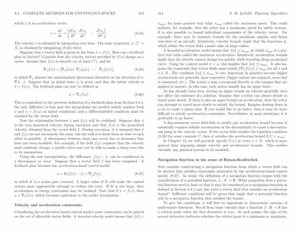
8.4. COMPLETE METHODS FOR CONTINUOUS SPACES 413
which x is an acceleration vector,
x =dx
dt=
[
d2x1dt2
d2x2dt2
· · · d2xndt2
]
. (8.44)
The velocity x is obtained by integration over time. The state trajectory, x : T →X, is obtained by integrating (8.44) twice.
Suppose that a vector field is given in the form x = f(x). How can a feedbackplan be derived? Consider how the velocity vectors specified by f(x) change as xvaries. Assume that f(x) is smooth (or at least C1), and let
∇xf(x) = [∇xf1(x) ∇xf2(x) · · · ∇xfn(x)] , (8.45)
in which ∇x denotes the unnormalized directional derivative in the direction of x:∇fi · x. Suppose that an initial state xI is given, and that the initial velocity isx = f(xI). The feedback plan can now be defined as
u = ∇xf(x). (8.46)
This is equivalent to the previous definition of a feedback plan from Section 8.4.1;the only difference is that now two integrations are needed (which requires bothx and x = f(xI) as initial conditions) and a differentiability condition must besatisfied for the vector field.
Now the relationship between x and f(x) will be redefined. Suppose that xis the true measured velocity during execution and that f(x) is the prescribedvelocity, obtained from the vector field f . During execution, it is assumed that xand f(x) are not necessarily the same, but the task is to keep them as close to eachother as possible. A discrepancy between them may occur due to dynamics thathave not been modeled. For example, if the field f(x) requests that the velocitymust suddenly change, a mobile robot may not be able to make a sharp turn dueto its momentum.
Using the new interpretation, the difference, f(x) − x, can be considered asa discrepancy or error. Suppose that a vector field f has been computed. Afeedback plan becomes the acceleration-based control model
u = K(f(x)− x) +∇xf(x), (8.47)
in which K is a scalar gain constant. A larger value of K will make the controlsystem more aggressively attempt to reduce the error. If K is too large, thenacceleration or energy constraints may be violated. Note that if x = f(x), thenu = ∇xf(x), which becomes equivalent to the earlier formulation.
Velocity and acceleration constraints
Considering the acceleration-based control model, some constraints can be placedon the set of allowable vector fields. A bounded-velocity model means that ‖x‖ <
414 S. M. LaValle: Planning Algorithms
vmax, for some positive real value vmax called the maximum speed. This couldindicate, for example, that the robot has a maximum speed for safety reasons.It is also possible to bound individual components of the velocity vector. Forexample, there may be separate bounds for the maximum angular and linearvelocities of an aircraft. Intuitively, velocity bounds imply that the functions fi,which define the vector field, cannot take on large values.
A bounded-acceleration model means that ‖x‖ ≤ amax, in which amax is a pos-itive real value called the maximum acceleration. Intuitively, acceleration boundsimply that the velocity cannot change too quickly while traveling along an integralcurve. Using the control model x = u, this implies that ‖u‖ ≤ amax. It also im-poses the constraint that vector fields must satisfy ‖∇xf(x)‖ ≤ amax for all x andx ∈ X. The condition ‖u‖ ≤ amax is very important in practice because higheraccelerations are generally more expensive (bigger motors are required, more fuelis consumed, etc.). The action u may correspond directly to the torques that areapplied to motors. In this case, each motor usually has an upper limit.
As has already been seen, setting an upper bound on velocity generally doesnot affect the existence of a solution. Imagine that a robot can always decide totravel more slowly. If there is also an upper bound on acceleration, then the robotcan attempt to travel more slowly to satisfy the bound. Imagine slowing down ina car to make a sharp turn. If you would like to go faster, then it may be moredifficult to satisfy acceleration constraints. Nevertheless, in most situations, it ispreferable to go faster.
A discontinuous vector field fails to satisfy any acceleration bound because itessentially requires infinite acceleration at the discontinuity to cause a discontinu-ous jump in the velocity vector. If the vector field satisfies the Lipschitz condition(8.16) for some constant C, then it satisfies the acceleration bound if C < amax.
In Chapter 13, we will precisely specify U(x) at every x ∈ X, which is moregeneral than imposing simple velocity and acceleration bounds. This enablesvirtually any physical system to be modeled.
Navigation function in the sense of Rimon-Koditschek
Now consider constructing a navigation function from which a vector field canbe derived that satisfies constraints motivated by the acceleration-based controlmodel, (8.47). As usual, the definition of a navigation function begins with theconsideration of a potential function, φ : X → R. What properties does a poten-tial function need to have so that it may be considered as a navigation function asdefined in Section 8.4.1 and also yield a vector field that satisfies an accelerationbound? Sufficient conditions will be given that imply that a potential functionwill be a navigation function that satisfies the bound.
To give the conditions, it will first be important to characterize extrema ofmultivariate functions. Recall from basic calculus that a function f : R→ R hasa critical point when the first derivative is zero. At such points, the sign of thesecond derivative indicates whether the critical point is a minimum or maximum.

8.4. COMPLETE METHODS FOR CONTINUOUS SPACES 415
These ideas can be generalized to higher dimensions. A critical point of φ is onefor which ∇φ = 0. The Hessian of φ is defined as the matrix
H(φ) =
∂2φ
∂2x21
∂2φ
∂x1∂x2· · · ∂2φ
∂x1∂xn
∂2φ
∂x2∂x1
∂2φ
∂x22· · · ∂2φ
∂x2∂xn
......
...
∂2φ
∂xn∂x1
∂2φ
∂xn∂x2· · · ∂2φ
∂x2n
. (8.48)
At each critical point, the Hessian gives some information about the extremum.If the rank of H(φ) at x is n, then the Hessian indicates the kind of extremum. If(8.48) is positive definite,13 then the φ achieves a local minimum at x. If (8.48) isnegative definite,14 then the φ achieves a local maximum at x. In all other cases,x is a saddle point. If the rank of H(φ) at x is less than n, then the Hessian isdegenerate. In this case the Hessian cannot classify the type of extremum. Anexample of this occurs when x lies in a plateau (there is no direction in whichφ increases or decreases. Such behavior is obviously bad for a potential functionbecause the local operator would not be able to select a direction.
Suppose that the navigation function is required to be smooth, to ensure theexistence of a gradient at every point. This enables gradient descent to be per-formed. If X is not contractible, then it turns out there must exist some criticalpoints other than xG at which ∇φ(x) = 0. The critical points can even be usedto infer the topology of X, which is the basic idea in the subject of Morse theory[366, 126]. Unfortunately, this implies that there does not exist a solution naviga-tion function for such spaces because the definition in Section 8.4.1 required thatthe integral curve from any state that can reach xG must reach it using the vectorfield derived from the navigation function. If the initial state is a critical point,the integral curve is constant (the state remains at the critical point). Therefore,under the smoothness constraint, the definition of a navigation function should bemodified to allow critical points at a small number of places (only on a set thathas measure zero). It is furthermore required that the set of states from whichthe integral curves arrive at each critical point (i.e., the domain of attraction ofeach critical point) has measure zero. From all possible initial states, except froma set of measure zero, the integral curves must reach xG, if it is reachable. Thisis ensured in the following definition.
13Positive definite for an n × n matrix A means that for all x ∈ Rn, xTAx > 0. If A issymmetric (which applies to H(φ)), then this is equivalent to A having all positive eigenvalues.
14Negative definite means that for all x ∈ Rn, xTAx < 0. If A is symmetric, then this isequivalent to A having all negative eigenvalues.
416 S. M. LaValle: Planning Algorithms
A function φ : X → R is called a navigation function in the sense of Rimon-Koditschek if [416]:
1. It is smooth (or at least C2).
2. Among all values on the connected component of Cfree that contains xG,there is only one local minimum, which is at xG.
15
3. It is maximal and constant on ∂Cfree, the boundary of Cfree.
4. It is a Morse function [366], which means that at each critical point x (i.e.,∇φ|x = 0), the Hessian of φ is not degenerate.16 Such functions are knownto exist on any smooth manifold.
If φ is smooth in the C∞ sense, then by Sard’s Theorem [126] the set of criticalpoints has measure zero.
Methods for constructing navigation functions are outlined in [416] for a gen-eral family of problems in which Cfree has a semi-algebraic description. The basicidea is to start with simple shapes over which a navigation function can be easilydefined. One example of this is a spherical subset of Rn, which contains sphericalobstacles. A set of distorting transformations is then developed to adapt the nav-igation functions to other shapes while ensuring that the four properties aboveare maintained. One such transformation extends a ball into any visibility region(in the sense defined in Section 8.4.3). This is achieved by smoothly stretchingout the ball into the shape of the visibility region. (Such regions are sometimescalled star-shaped.) The transformations given in [416] can be combined to definenavigation functions for a large family of configuration spaces. The main problemis that the configuration space obstacles and the connectivity of Cfree are repre-sented only implicitly, which makes it difficult to correctly apply the method tocomplicated high-dimensional problems. One of the advantages of the approachis that proving convergence to the goal is simplified. In many cases, Lyapunovstability analysis can be performed (see Section 15.1.1).
Harmonic potential functions
Another important family of navigation functions is constructed from harmonicfunctions [128, 129, 130, 250, 276]. A function φ is called a harmonic function ifit satisfies the differential equation
∇2φ =n∑
i=1
∂2φ
∂x2i= 0. (8.49)
15Some authors do not include the global minimum as a local minimum. In this case, onewould say that there are no local minima.
16Technically, to be Morse, the values of the function must also be distinct at each criticalpoint.

8.5. SAMPLING-BASED METHODS FOR CONTINUOUS SPACES 417
There are many possible solutions to the equation, depending on the conditionsalong the boundary of the domain over which φ is defined. A simple disc-basedexample is given in [127] for which an analytical solution exists. Complicatednavigation functions are generally defined by imposing constraints on φ along theboundary of Cfree. A Dirichlet boundary condition means that the boundary mustbe held to a constant value. Using this condition, a harmonic navigation functioncan be developed that guides the state into a goal region from anywhere in a simplyconnected state space. If there are interior obstacles, then a Neumann boundarycondition forces the velocity vectors to be tangent to the obstacle boundary. Bysolving (8.49) under a combination of both boundary conditions, a harmonic nav-igation function can be constructed that avoids obstacles by moving parallel totheir boundaries and eventually landing in the goal. It has been shown undergeneral conditions that navigation functions can be produced [130, 129]; however,the main problems are that the boundary of Cfree is usually not constructed ex-plicitly (recall why this was avoided in Chapter 5) and that a numerical solutionto (8.49) is expensive to compute. This can be achieved, for example, by usingGauss-Seidel iterations (as indicated in [130]), which are related to value iteration(see [59] for the distinction). A sampling-based approach to constructing naviga-tion functions via harmonic functions is presented in [68]. Value iteration will beused to produce approximate, optimal navigation functions in Section 8.5.2.
8.5 Sampling-Based Methods for Continuous Spaces
The methods in Section 8.4 can be considered as the feedback-case analogs tothe combinatorial methods of Chapter 6. Although such methods provide elegantsolutions to the problem, the issue arises once again that they are either limited tolower dimensional problems or problems that exhibit some special structure. Thismotivates the introduction of sampling-based methods. This section presents thefeedback-case analog to Chapter 5.
8.5.1 Computing a Composition of Funnels
Mason introduced the concept of a funnel as a metaphor for motions that convergeto the same small region of the state space, regardless of the initial position [351].As grains of sand in a funnel, they follow the slope of the funnel until they reachthe opening at the bottom. A navigation function can be imagined as a funnelthat guides the state into the goal. For example, the cost-to-go function depictedin Figure 8.13d can be considered as a complicated funnel that sends each pieceof sand along an optimal path to the goal.
Rather than designing a single funnel, consider decomposing the state spaceinto a collection of simple, overlapping regions. Over each region, a funnel can bedesigned that leads the state into another funnel; see Figure 8.14. As an example,the approach in [83] places a Lyapunov function (such functions are covered in
418 S. M. LaValle: Planning Algorithms
1 2 3
1
3
2
Figure 8.14: A navigation function and corresponding vector field can be designedas a composition of funnels.
X
X
Figure 8.15: An approximate cover is shown. Every point of X is contained in atleast one neighborhood, and X is a subset of X.
Section 15.1.2) over each funnel to ensure convergence to the next funnel. Afeedback plan can be constructed by composing several funnels. Starting fromsome initial state in X, a sequence of funnels is visited until the goal is reached.Each funnel essentially solves the subgoal of reaching the next funnel. Eventually,a funnel is reached that contains the goal, and a navigation function on this funnelcauses the goal to be reached. In the context of sensing uncertainty, for which thefunnel metaphor was developed, the composition of funnels becomes the preimageplanning framework [346], which is covered in Section 12.5.1. In this section,however, it is assumed that the current state is always known.
An approximate cover
Figure 8.15 illustrates the notion of an approximate cover, which will be used torepresent the funnel domains. Let X denote a subset of a state space X. A coverof X is a collection O of sets for which

8.5. SAMPLING-BASED METHODS FOR CONTINUOUS SPACES 419
1. O ⊆ X for each O ∈ O.
2. X is a subset of the union of all sets in the cover:
X ⊆⋃
O∈OO. (8.50)
Let each O ∈ O be called a neighborhood. The notion of a cover was actuallyused in Section 8.3.2 to define a smooth manifold using a cover of coordinateneighborhoods.
In general, a cover allows the following:
1. Any number of neighborhoods may overlap (have nonempty intersection).
2. Any neighborhood may contain points that lie outside of X.
A cell decomposition, which was introduced in Section 6.3.1, is a special kindof cover for which the neighborhoods form a partition of X, and they must fittogether nicely (recall Figure 6.15).
So far, no constraints have been placed on the neighborhoods. They shouldbe chosen in practice to greatly simplify the design of a navigation function overeach one. For the original motion planning problem, cell decompositions weredesigned to make the determination of a collision-free path trivial in each cell.The same idea applies here, except that we now want to construct a feedbackplan. Therefore, it is usually assumed that the cells have a simple shape.
A cover is called approximate if X is a strict subset of X. Ideally, we wouldlike to develop an exact cover, which implies that X = X and each neighborhoodhas some nice property, such as being convex. Developing such covers is possiblein practice for state spaces that are either low-dimensional or exhibit some specialstructure. This was observed for the cell decomposition methods of Chapter 6.
Consider constructing an approximate cover for X. The goal should be tocover as much of X as possible. This means that µ(X \ X) should be made assmall as possible, in which µ denotes Lebesgue measure, as defined in Section5.1.3. It is also desirable to ensure that X preserves the connectivity of X. Inother words, if a path between two points exists in X, then it should also exist inX.
Defining a feedback plan over a cover
The ideas from Section 8.4.2 can be adapted to define a feedback plan over Xusing a cover. Let X denote a discrete state space in which each superstateis a neighborhood. Most of the components of the associated discrete planningproblems are the same as in Section 8.4.2. The only difference is in the definition ofsuperactions because neighborhoods can overlap in a cover. For each neighborhoodO ∈ O, a superaction exists for each other neighborhood, O′ ∈ O such thatO ∩O′ 6= ∅ (usually, their interiors overlap to yield int(O) ∩ int(O′) 6= ∅).
420 S. M. LaValle: Planning Algorithms
O′O
Figure 8.16: A transition from O to O′ is caused by a vector field on O for whichall integral curves lead into O ∩O′.
Note that in the case of a cell decomposition, this produces no superactionsbecause it is a partition. To follow the metaphor of composing funnels, the do-mains of some funnels should overlap, as shown in Figure 8.14. A transition fromone neighborhood, O, to another, O′, is obtained by defining a vector field on Othat sends all states from O \O′ into O∩O′; see Figure 8.16. Once O′ is reached,the vector field of O is no longer followed; instead, the vector field of O′ is used.Using the vector field of O′, a transition may be applied to reach another neigh-borhood. Note that the jump from the vector field of O to that of O′ may causethe feedback plan to be a discontinuous vector field on X. If the cover is designedso that O∩O′ is large (if they intersect), then gradual transitions may be possibleby blending the vector fields from O and O′.
Once the discrete problem has been defined, a discrete feedback plan can becomputed over X, as defined in Section 8.2. This is converted into a feedbackplan over X by defining a vector field on each neighborhood that causes theappropriate transitions. Each x ∈ X can be interpreted both as a superstate anda neighborhood. For each x, the discrete feedback plan produces a superactionu = π(x), which yields a new neighborhood x′. The vector field over x = O isthen designed to send all states into x′ = O′.
If desired, a navigation function φ overX can even be derived from a navigationfunction, φ, over X. Suppose that φ is constructed so that every φ(x) is distinctfor every x ∈ X. Any navigation function can be easily transformed to satisfy thisconstraint (because X is finite). Let φO denote a navigation function over someO ∈ O. Assume that XG is a point, xG (extensions can be made to more generalcases). For every neighborhood O ∈ O such that xG 6∈ O, φO is defined so thatperforming gradient descent leads into the overlapping neighborhood for whichφ(x) is smallest. If O contains xG, the navigation function φO simply guides thestate to xG.
The navigation functions over each O ∈ O can be easily pieced together toyield a navigation function over all of X. In places where multiple neighborhoodsoverlap, φ is defined to be the navigation function associated with the neighbor-

8.5. SAMPLING-BASED METHODS FOR CONTINUOUS SPACES 421
hood for which φ(x) is smallest. This can be achieved by adding a large constantto each φO. Let c denote a constant for which φO(x) < c over all O ∈ O and x ∈ O(it is assumed that each φO is bounded). Suppose that φ assumes only integervalues. Let O(x) denote the set of all O ∈ O such that x ∈ O. The navigationfunction over X is defined as
φ(x) = minO∈O(x)
φO(x) + c φ(O)
. (8.51)
A sampling-based approach
There are numerous alternative ways to construct a cover. To illustrate the ideas,an approach called the sampling-based neighborhood graph is presented here [480].Suppose that X = Cfree, which is a subset of some configuration space. As intro-duced in Section 5.4, let α be a dense, infinite sequence of samples in X. Assumethat a collision detection algorithm is available that returns the distance, (5.28),between the robot and obstacles in the world. Such algorithms were described inSection 5.3.
An incremental algorithm is given in Figure 8.17. Initially, O is empty. In eachiteration, if α(i) ∈ Cfree and it is not already contained in some neighborhood,then a new neighborhood is added to O. The two main concerns are 1) how todefine a new neighborhood, O, such that O ⊂ Cfree, and 2) when to terminate. Atany given time, the cover is approximate. The union of all neighborhoods is X,which is a strict subset of X. In comparison to Figure 8.15, the cover is a specialcase in which the neighborhoods do not extend beyond X.
Defining new neighborhoods For defining new neighborhoods, it is importantto keep them simple because during execution, the neighborhoods that containthe state x must be determined quickly. Suppose that all neighborhoods are openballs:
B(x, r) = x′ ∈ X | ρ(x, x′) < r, (8.52)
in which ρ is the metric on C. There are efficient algorithms for determiningwhether x ∈ O for some O ∈ O, assuming all of the neighborhoods are balls [365].In practice, methods based on Kd-trees yield good performance [36, 38] (recallSection 5.5.2). A new ball, B(x, r), can be constructed in Step 3 for x = α(i),but what radius can be assigned? For a point robot that translates in R2 or R3,the Hausdorff distance d between the robot and obstacles in W is precisely thedistance to Cobs from α(i). This implies that we can set r = d, and B(x, r) isguaranteed to be collision-free.
In a general configuration space, it is possible to find a value of r such thatB(x, r) ⊆ Cfree, but in general r < d. This issue arose in Section 5.3.4 for checkingpath segments. The transformations of Sections 3.2 and 3.3 become importantin the determination of r. For illustrative purposes, suppose that C = R2 × S1,
422 S. M. LaValle: Planning Algorithms
INCREMENTAL COVER CONSTRUCTION
1. Initialize O = ∅ and i = 1.
2. Let x = α(i), and let d be the distance returned by the collision detectionalgorithm applied at x.
3. If d > 0 (which implies that x ∈ Cfree) and x 6∈ O for all O ∈ O, theninsert a new neighborhood, On, into O. The neighborhood size and shapeare determined from x and d.
4. If the termination condition is not satisfied, then let i := i + 1, and go toStep 1.
5. Remove any neighborhoods from O that are contained entirely inside ofanother neighborhood.
Figure 8.17: The cover is incrementally extended by adding new neighborhoodsthat are guaranteed to be collision-free.
which corresponds to a rigid robot, A, that can translate and rotate in W = R2.Each point a ∈ A is transformed using (3.35). Now imagine starting with someconfiguration q = (x, y, θ) and perturbing each coordinate by some ∆x, ∆y, and∆θ. What is the maximum distance that a point on A could travel? Translationaffects all points on A the same way, but rotation affects points differently. RecallFigure 5.12 from Section 5.3.4. Let ar ∈ A denote the point that is furthest fromthe origin (0, 0). Let r denote the distance from ar to the origin. If the rotationis perturbed by some small amount, ∆θ, then the displacement of any a ∈ A isno more than r∆θ. If all three configuration parameters are perturbed, then
(∆x)2 + (∆y)2 + (r∆θ)2 < d2 (8.53)
is the constraint that must be satisfied to ensure that the resulting ball is containedin Cfree. This is actually the equation of a solid ellipsoid, which becomes a ball ifr = 1. This can be made into a ball by reparameterizing SE(2) so that ∆θ hasthe same affect as ∆x and ∆y. A transformation h : θ 7→ rθ maps θ into a newdomain Z = [0, 2πr). In this new space, the equation of the ball is
(∆x)2 + (∆y)2 + (∆z)2 < d2, (8.54)
in which ∆z represents the change in z ∈ Z. The reparameterized version of(3.35) is
T =
cos(θ/r) − sin(θ/r) xtsin(θ/r) cos(θ/r) yt
0 0 1
. (8.55)

8.5. SAMPLING-BASED METHODS FOR CONTINUOUS SPACES 423
For a 3D rigid body, similar reparameterizations can be made to Euler angles orquaternions to generate six-dimensional balls. Extensions can be made to chainsof bodies [480]. One of the main difficulties, however, is that the balls are notthe largest possible. In higher dimensions the problem becomes worse becausenumerous balls are needed, and the radii constructed as described above tend tobe much smaller than what is possible. The number of balls can be reduced byalso allowing axis-aligned cylinders, but it still remains difficult to construct acover over a large fraction of Cfree in more than six dimensions.
Termination The sampling-based planning algorithms in Chapter 5 were de-signed to terminate upon finding a solution path. In the current setting, ter-mination is complicated by the fact that we are interested in solutions from allinitial configurations. Since α is dense, the volume of uncovered points in Cfreetends to zero. After some finite number of iterations, it would be nice to measurethe quality of the approximation and then terminate when the desired quality isachieved. This was also possible with the visibility sampling-based roadmap inSection 5.6.2. Using random samples, an estimate of the fraction of Cfree can beobtained by recording the percentage of failures in obtaining a sample in Cfreethat is outside of the cover. For example, if a new neighborhood is created onlyonce in 1000 iterations, then it can be estimated that 99.9 percent of Cfree is cov-ered. High-probability bounds can also be determined. Termination conditionsare given in [480] that ensure with probability greater than Pc that at least afraction α ∈ (0, 1) of Cfree has been covered. The constants Pc and α are given asparameters to the algorithm, and it will terminate when the condition has beensatisfied using rigorous statistical tests. If deterministic sampling is used, thentermination can be made to occur based on the dispersion, which indicates thelargest ball in Cfree that does not contain the center of another neighborhood. Oneproblem with volume-based criteria, such as those suggested here, is that there isno way to ensure that the cover preserves the connectivity of Cfree. If two portionsof Cfree are connected by a narrow passage, the cover may miss a neighborhoodthat has very small volume yet is needed to connect the two portions.
Example 8.18 (2D Example of Computed Funnels) Figure 8.18 shows a 2Dexample that was computed using random samples and the algorithm in Figure8.17. Note that once a cover is computed, it can be used to rapidly computedifferent navigation functions and vector fields for various goals. This example ismainly for illustrative purposes. For the case of a polygonal environment, con-structing covers based on convex polygons would be more efficient.
424 S. M. LaValle: Planning Algorithms
(a) (b)
Figure 8.18: (a) A approximate cover for a 2D configuration space. (b) Level setsof a navigation function.
8.5.2 Dynamic Programming with Interpolation
This section concludes Part II by solving the motion planning problem with valueiteration, which was introduced in Section 2.3. It has already been applied toobtain discrete feedback plans in Section 8.2. It will now be adapted to continuousspaces by allowing interpolation first over a continuous state space and then byadditionally allowing interpolation over a continuous action space. This yieldsa numerical approach to computing optimal navigation functions and feedbackplans for motion planning. The focus will remain on backward value iteration;however, the interpolation concepts may also be applied in the forward direction.The approach here views optimal feedback motion planning as a discrete-timeoptimal control problem [22, 55, 79, 302].
Using interpolation for continuous state spaces
Consider a problem formulation that is identical to Formulation 8.1 except thatX is allowed to be continuous. Assume that X is bounded, and assume for nowthat the action space, U(x), it finite for all x ∈ X. Backward value iteration canbe applied. The dynamic programming arguments and derivation are identical tothose in Section 2.3. The resulting recurrence is identical to (2.11) and is repeatedhere for convenience:
G∗k(xk) = min
uk∈U(xk)
l(xk, uk) +G∗k+1(xk+1)
. (8.56)

8.5. SAMPLING-BASED METHODS FOR CONTINUOUS SPACES 425
xk
Stage k + 1
Stage k
Possible next states
Figure 8.19: Even though xk is a sample point, the next state, xk+1, may landbetween sample points. For each uk ∈ U(xk), interpolation may be needed for theresulting next state, xk+1 = f(xk, uk).
The only difficulty is that G∗k(xk) cannot be stored for every xk ∈ X because X is
continuous. There are two general approaches. One is to approximate G∗k using
a parametric family of surfaces, such as polynomials or nonlinear basis functionsderived from neural networks [60]. The other is to store G∗
k only over a finiteset of sample points and use interpolation to obtain its value at all other points[301, 302].
Suppose that a finite set S ⊂ X of samples is used to represent cost-to-gofunctions overX. The evaluation of (8.56) using interpolation is depicted in Figure8.19. In general, the samples should be chosen to reduce the dispersion (definedin Section 5.2.3) as much as possible. This prevents attempts to approximatethe cost-to-go function on large areas that contain no sample points. The rateof convergence ultimately depends on the dispersion [58] (in combination withLipschitz conditions on the state transition equation and the cost functional).To simplify notation and some other issues, assume that S is a grid of regularlyspaced points in Rn.
First, consider the case in which X = [0, 1] ⊂ R. Let S = s0, s1, . . . , sr,in which si = i/r. For example, if r = 3, then S = 0, 1/3, 2/3, 1. Note thatthis always yields points on the boundary of X, which ensures that for any pointin (0, 1) there are samples both above and below it. Let i be the largest integersuch that si < x. This implies that si+1 > x. The samples si and si+1 are calledinterpolation neighbors of x.
The value of G∗k+1 in (8.56) at any x ∈ [0, 1] can be obtained via linear inter-
polation asG∗
k+1(x) ≈ αG∗k+1(si) + (1− α)G∗
k+1(si+1), (8.57)
in which the coefficient α ∈ [0, 1] is computed as
α = 1− x− sir
. (8.58)
If x = si, then α = 1, and (8.57) reduces to G∗k+1(si), as expected. If x = si+1,
then α = 0, and (8.57) reduces to G∗k+1(si+1). At all points in between, (8.57)
blends the cost-to-go values at si and si+1 using α to provide the appropriateweights.
The interpolation idea can be naturally extended to multiple dimensions. LetX be a bounded subset of Rn. Let S represent an n-dimensional grid of points
426 S. M. LaValle: Planning Algorithms
n = 2 n = 3
Figure 8.20: Barycentric subdivision can be used to partition each cube intosimplexes, which allows interpolation to be performed in O(n lg n) time, insteadof O(2n).
in Rn. Each sample in S is denoted by s(i1, i2, . . . , in). For some x ∈ X, thereare 2n interpolation neighbors that “surround” it. These are the corners of ann-dimensional cube that contains x. Let x = (x1, . . . , xn). Let ij denote thelargest integer for which the jth coordinate of s(i1, i2, . . . , in) is less than xj. The2n samples are all those for which either ij or ij + 1 appears in the expressions(·, ·, . . . , ·), for each j ∈ 1, . . . , n. This requires that samples exist in S for allof these cases. Note that X may be a complicated subset of Rn, provided that forany x ∈ X, all of the required 2n interpolation neighbors are in S. Using the 2n
interpolation neighbors, the value of G∗k+1 in (8.56) on any x ∈ X can be obtained
via multi-linear interpolation. In the case of n = 2, this is expressed as
G∗k+1(x) ≈ α1α2 G
∗k+1(s(i1, i2))+
α1(1− α2) G∗k+1(s(i1, i2 + 1))+
(1− α1)α2 G∗k+1(s(i1 + 1, i2))+
(1− α1)(1− α2) G∗k+1(s(i1 + 1, i2 + 1)),
(8.59)
in which α1 and α2 are defined similarly to α in (8.58) but are based on distancesalong the x1 and x2 directions, respectively. The expressions for multi-linear in-terpolation in higher dimensions are similar but are more cumbersome to express.Higher order interpolation, such a quadratic interpolation may alternatively beused [302].
Unfortunately, the number of interpolation neighbors grows exponentially withthe dimension, n. Instead of using all 2n interpolation neighbors, one improvementis to decompose the cube defined by the 2n samples into simplexes. Each simplexhas only n+1 samples as its vertices. Only the vertices of the simplex that contains
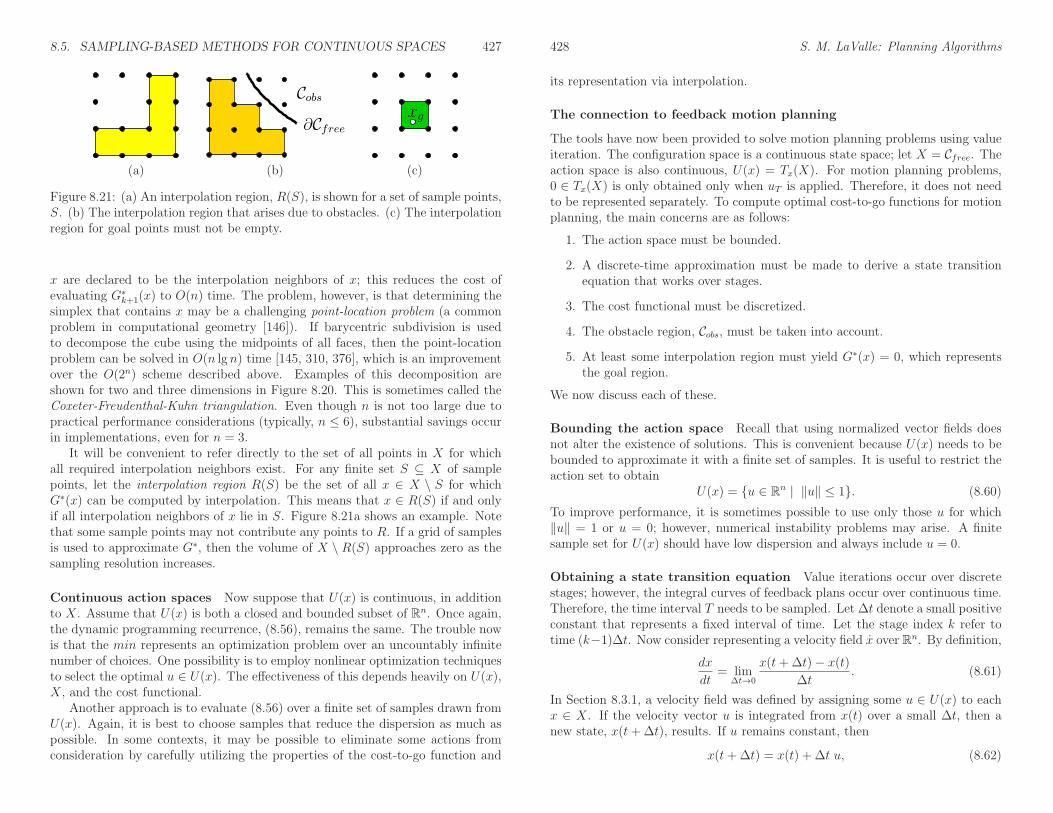
8.5. SAMPLING-BASED METHODS FOR CONTINUOUS SPACES 427
Cobs
∂Cfree
xg
(a) (b) (c)
Figure 8.21: (a) An interpolation region, R(S), is shown for a set of sample points,S. (b) The interpolation region that arises due to obstacles. (c) The interpolationregion for goal points must not be empty.
x are declared to be the interpolation neighbors of x; this reduces the cost ofevaluating G∗
k+1(x) to O(n) time. The problem, however, is that determining thesimplex that contains x may be a challenging point-location problem (a commonproblem in computational geometry [146]). If barycentric subdivision is usedto decompose the cube using the midpoints of all faces, then the point-locationproblem can be solved in O(n lg n) time [145, 310, 376], which is an improvementover the O(2n) scheme described above. Examples of this decomposition areshown for two and three dimensions in Figure 8.20. This is sometimes called theCoxeter-Freudenthal-Kuhn triangulation. Even though n is not too large due topractical performance considerations (typically, n ≤ 6), substantial savings occurin implementations, even for n = 3.
It will be convenient to refer directly to the set of all points in X for whichall required interpolation neighbors exist. For any finite set S ⊆ X of samplepoints, let the interpolation region R(S) be the set of all x ∈ X \ S for whichG∗(x) can be computed by interpolation. This means that x ∈ R(S) if and onlyif all interpolation neighbors of x lie in S. Figure 8.21a shows an example. Notethat some sample points may not contribute any points to R. If a grid of samplesis used to approximate G∗, then the volume of X \ R(S) approaches zero as thesampling resolution increases.
Continuous action spaces Now suppose that U(x) is continuous, in additionto X. Assume that U(x) is both a closed and bounded subset of Rn. Once again,the dynamic programming recurrence, (8.56), remains the same. The trouble nowis that the min represents an optimization problem over an uncountably infinitenumber of choices. One possibility is to employ nonlinear optimization techniquesto select the optimal u ∈ U(x). The effectiveness of this depends heavily on U(x),X, and the cost functional.
Another approach is to evaluate (8.56) over a finite set of samples drawn fromU(x). Again, it is best to choose samples that reduce the dispersion as much aspossible. In some contexts, it may be possible to eliminate some actions fromconsideration by carefully utilizing the properties of the cost-to-go function and
428 S. M. LaValle: Planning Algorithms
its representation via interpolation.
The connection to feedback motion planning
The tools have now been provided to solve motion planning problems using valueiteration. The configuration space is a continuous state space; let X = Cfree. Theaction space is also continuous, U(x) = Tx(X). For motion planning problems,0 ∈ Tx(X) is only obtained only when uT is applied. Therefore, it does not needto be represented separately. To compute optimal cost-to-go functions for motionplanning, the main concerns are as follows:
1. The action space must be bounded.
2. A discrete-time approximation must be made to derive a state transitionequation that works over stages.
3. The cost functional must be discretized.
4. The obstacle region, Cobs, must be taken into account.
5. At least some interpolation region must yield G∗(x) = 0, which representsthe goal region.
We now discuss each of these.
Bounding the action space Recall that using normalized vector fields doesnot alter the existence of solutions. This is convenient because U(x) needs to bebounded to approximate it with a finite set of samples. It is useful to restrict theaction set to obtain
U(x) = u ∈ Rn | ‖u‖ ≤ 1. (8.60)
To improve performance, it is sometimes possible to use only those u for which‖u‖ = 1 or u = 0; however, numerical instability problems may arise. A finitesample set for U(x) should have low dispersion and always include u = 0.
Obtaining a state transition equation Value iterations occur over discretestages; however, the integral curves of feedback plans occur over continuous time.Therefore, the time interval T needs to be sampled. Let ∆t denote a small positiveconstant that represents a fixed interval of time. Let the stage index k refer totime (k−1)∆t. Now consider representing a velocity field x over Rn. By definition,
dx
dt= lim
∆t→0
x(t+∆t)− x(t)∆t
. (8.61)
In Section 8.3.1, a velocity field was defined by assigning some u ∈ U(x) to eachx ∈ X. If the velocity vector u is integrated from x(t) over a small ∆t, then anew state, x(t+∆t), results. If u remains constant, then
x(t+∆t) = x(t) + ∆t u, (8.62)
8.5. SAMPLING-BASED METHODS FOR CONTINUOUS SPACES 429
which is called an Euler approximation. If a feedback plan is executed, then u isdetermined from x via u = π(x(t)). In general, this means that u could vary asthe state is integrated forward. In this case, (8.62) is only approximate,
x(t+∆t) ≈ x(t) + ∆t π(x(t)). (8.63)
The expression in (8.62) can be considered as a state transition equation thatworks over stages. Let xk+1 = x(t +∆t) and xk = x(t). The transitions can nowbe expressed as
xk+1 = f(xk, u) = xk +∆t u. (8.64)
The quality of the approximation improves as ∆t decreases. Better approxi-mations can be made by using more sample points along time. The most widelyknown approximations are the Runge-Kutta family. For optimal motion planning,it turns out that the direction vector almost always remains constant along the in-tegral curve. For example, in Figure 8.13d, observe that piecewise-linear paths areobtained by performing gradient descent of the optimal navigation function. Thedirection vector is constant over most of the resulting integral curve (it changesonly as obstacles are contacted). Therefore, approximation problems tend notto arise in motion planning problems. When approximating dynamical systems,such as those presented in Chapter 13, then better approximations are needed;see Section 14.3.2. One important concern is that ∆t is chosen in a way thatis compatible with the grid resolution. If ∆t is so small that the actions do notchange the state enough to yield new interpolation neighbors, then the interpo-lated cost-to-go values will remain constant. This implies that ∆t must be chosento ensure that x(t+∆t) has a different set of interpolation neighbors than x(t).
An interesting connection can be made to the approximate motion planningproblem that was developed in Section 7.7. Formulation 7.4 corresponds pre-cisely to the approximation defined here, except that ǫ was used instead of ∆tbecause velocities were not yet considered (also, the initial condition was speci-fied because there was no feedback). Recall the different possible action spacesshown in Figure 7.41. As stated in Section 7.7, if the Manhattan or independent-joint models are used, then the configurations remain on a grid of points. Thisenables discrete value iterations to be performed. A discrete feedback plan andnavigation function, as considered in Section 8.2.3, can even be computed. If theEuclidean motion model is used, which is more natural, then the transitions allowa continuum of possible configurations. This case can finally be handled by usinginterpolation over the configuration space, as described in this section.
Approximating the cost functional A discrete cost functional must be de-rived from the continuous cost functional, (8.39). The final term is just assignedas lF (xF ) = lF (x(tf )). The cost at each stage is
ld(xk, uk) =
∫ ∆t
0
l(x(t), u(t))dt, (8.65)
430 S. M. LaValle: Planning Algorithms
and ld(xk, uk) is used in the place of l(xk, uk) in (8.56). For many problems, theintegral does not need to be computed repeatedly. To obtain Euclidean shortestpaths, ld(xk, uk) = ‖uk‖ can be safely assigned for all xk ∈ X and uk ∈ U(xk). Areasonable approximation to (8.65) if ∆t is small is l(x(t), u(t))∆t.
Handling obstacles A simple way to handle obstacles is to determine for eachx ∈ S whether x ∈ Cobs. This can be computed and stored in an array before thevalue iterations are performed. For rigid robots, this can be efficiently computedusing fast Fourier transforms [262]. For each x ∈ Cobs, G∗(x) = ∞. No valueiterations are performed on these states; their values must remain at infinity.During the evaluation of (8.59) (or a higher dimensional version), different actionsare attempted. For each action, it is required that all of the interpolation neighborsof xk+1 lie in Cfree. If one of them lies in Cobs, then that action produces infinitecost. This has the effect of automatically reducing the interpolation region, R(S),to all cubes whose vertices all lie in Cfree, as shown in Figure 8.21b. All samples inCobs are assumed to be deleted from S in the remainder of this section; however,the full grid is still used for interpolation so that infinite values represent theobstacle region.
Note that as expressed so far, it is possible that points in Cobs may lie in R(S)because collision detection is performed only on the samples. In practice, eitherthe grid resolution must be made fine enough to minimize the chance of this erroroccurring or distance information from a collision detection algorithm must beused to infer that a sufficiently large ball around each sample is collision free. Ifan interpolation region cannot be assured to lie in Cfree, then the resolution mayhave to be increased, at least locally.
Handling the goal region Recall that backward value iterations start withthe final cost-to-go function and iterate backward. Initially, the final cost-to-gois assigned as infinity at all states except those in the goal. To properly initializethe final cost-to-go function, there must exist some subset of X over which thezero value can be obtained by interpolation. Let G = S ∩XG. The requirementis that the interpolation region R(G) must be nonempty. If this is not satisfied,then the grid resolution needs to be increased or the goal set needs to be enlarged.If Xg is a single point, then it needs to be enlarged, regardless of the resolution(unless an alternative way to interpolate near a goal point is developed). In theinterpolation region shown in Figure 8.21c, all states in the vicinity of xG yield aninterpolated cost-to-go value of zero. If such a region did not exist, then all costswould remain at infinity during the evaluation of (8.59) from any state. Note that∆t must be chosen large enough to ensure that new samples can reach G.
Using G∗ as a navigation function After the cost-to-go values stabilize, theresulting cost-to-go function, G∗ can be used as a navigation function. Eventhough G∗ is defined only over S ⊂ X, the value of the navigation function can

8.5. SAMPLING-BASED METHODS FOR CONTINUOUS SPACES 431
be obtained using interpolation over any point in R(S). The optimal action isselected as the one that satisfies the min in (8.6). This means that the statetrajectory does not have to visit the grid points as in the Manhattan model. Atrajectory can visit any point in R(S), which enables trajectories to converge tothe true optimal solution as ∆t and the grid spacing tend to zero.
Topological considerations So far there has been no explicit consideration ofthe topology of C. Assuming that C is a manifold, the concepts discussed so far canbe applied to any open set on which coordinates are defined. In practice, it is oftenconvenient to use the manifold representations of Section 4.1.2. The manifold canbe expressed as a cube, [0, 1]n, with some faces identified to obtain [0, 1]n/ ∼. Overthe interior of the cube, all of the concepts explained in this section work withoutmodification. At the boundary, the samples used for interpolation must take theidentification into account. Furthermore, actions, uk, and next states, xk+1, mustfunction correctly on the boundary. One must be careful, however, in declaringthat some solution is optimal, because Euclidean shortest paths depend on themanifold parameterization. This ambiguity is usually resolved by formulating thecost in terms of some physical quantity, such as time or energy. This often requiresmodeling dynamics, which will be covered in Part IV.
Value iteration with interpolation is extremely general. It is a generic al-gorithm for approximating the solution to optimal control problems. It can beapplied to solve many of the problems in Part IV by restricting U(x) to take intoaccount complicated differential constraints. The method can also be extended toproblems that involve explicit uncertainty in predictability. This version of valueiteration is covered in Section 10.6.
Obtaining Dijkstra-like algorithms
For motion planning problems, it is expected that x(t + ∆t), as computed from(8.62), is always close to x(t) relative to the size of X. This suggests the useof a Dijkstra-like algorithm to compute optimal feedback plans more efficiently.As discussed for the finite case in Section 2.3.3, many values remain unchangedduring the value iterations, as indicated in Example 2.5. Dijkstra’s algorithmmaintains a data structure that focuses the computation on the part of the statespace where values are changing. The same can be done for the continuous caseby carefully considering the sample points [310].
During the value iterations, there are three kinds of sample points, just as inthe discrete case (recall from Section 2.3.3):
1. Dead: The cost-to-go has stabilized to its optimal value.
2. Alive: The current cost-to-go is finite, but it is not yet known whether thevalue is optimal.
432 S. M. LaValle: Planning Algorithms
3. Unvisited: The cost-to-go value remains at infinity because the sample hasnot been reached.
The sets are somewhat harder to maintain for the case of continuous state spacesbecause of the interaction between the sample set S and the interpolated regionR(S).
Imagine the first value iteration. Initially, all points in G are set to zero values.Among the collection of samples S, how many can reach R(G) in a single stage?We expect that samples very far from G will not be able to reach R(G); this keepstheir values are infinity. The samples that are close to G should reach it. It wouldbe convenient to prune away from consideration all samples that are too far fromG to lower their value. In every iteration, we eliminate iterating over samples thatare too far away from those already reached. It is also unnecessary to iterate overthe dead samples because their values no longer change.
To keep track of reachable samples, it will be convenient to introduce thenotion of a backprojection, which will be studied further in Section 10.1. For asingle state, x ∈ X, its backprojection is defined as
B(x) = x′ ∈ X | ∃u′ ∈ U(x′) such that x = f(x′, u′). (8.66)
The backprojection of a set, X ′ ⊆ X, of points is just the union of backprojectionsfor each point:
B(X ′) =⋃
x∈X′
B(x). (8.67)
Now consider a version of value iteration that uses backprojections to elimi-nate some states from consideration because it is known that their values cannotchange. Let i refer to the number of stages considered by the current value itera-tion. During the first iteration, i = 1, which means that all one-stage trajectoriesare considered. Let S be the set of samples (assuming already that none lie inCobs). Let Di and Ai refer to the dead and alive samples, respectively. Initially,D1 = G, the set of samples in the goal set. The first set, A1, of alive samples isassigned by using the concept of a frontier. The frontier of a set S ′ ⊆ S of samplepoints is
Front(S ′) = (B(R(S ′)) \ S ′) ∩ S. (8.68)
This is the set of sample points that can reach R(S ′) in one stage, excluding thosealready in S ′. Figure 8.22 illustrates the frontier. Using (8.68), A1 is defined asA1 = Front(D1).
Now the approach is described for iteration i. The cost-to-go update (8.56) iscomputed at all points inAi. IfG
∗k+1(s) = G∗
k(s) for some s ∈ Ai, then s is declareddead and moved to Di+1. Samples are never removed from the dead set; therefore,all points in Di are also added to Di+1. The next active set, Ai+1, includes allsamples in Ai, excluding those that were moved to the dead set. Furthermore,all samples in Front(Ai) are added to Ai+1 because these will produce a finitecost-to-go value in the next iteration. The iterations continue as usual until some
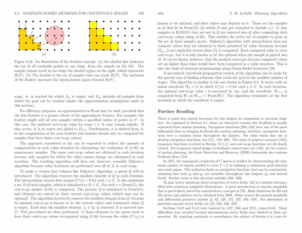
8.5. SAMPLING-BASED METHODS FOR CONTINUOUS SPACES 433
s
(a) (b)
Figure 8.22: An illustration of the frontier concept: (a) the shaded disc indicatesthe set of all reachable points in one stage, from the sample on the left. Thesample cannot reach in one stage the shaded region on the right, which representsR(S ′). (b) The frontier is the set of samples that can reach R(S ′). The inclusionof the frontier increases the interpolation region beyond R(S ′).
stage, m, is reached for which Am is empty, and Dm includes all samples fromwhich the goal can be reached (under the approximation assumptions made inthis section).
For efficiency purposes, an approximation to Front may be used, provided thatthe true frontier is a proper subset of the approximate frontier. For example, thefrontier might add all new samples within a specified radius of points in S ′. Inthis case, the updated cost-to-go value for some s ∈ Ai may remain infinite. Ifthis occurs, it is of course not added to Di+1. Furthermore, it is deleted from Ai
in the computation of the next frontier (the frontier should only be computed forsamples that have finite cost-to-go values).
The approach considered so far can be expected to reduce the amount ofcomputations in each value iteration by eliminating the evaluation of (8.56) onunnecessary samples. The same cost-to-go values are obtained in each iterationbecause only samples for which the value cannot change are eliminated in eachiteration. The resulting algorithm still does not, however, resemble Dijkstra’salgorithm because value iterations are performed over all of Ai in each stage.
To make a version that behaves like Dijkstra’s algorithm, a queue Q will beintroduced. The algorithm removes the smallest element of Q in each iteration.The interpolation version first assigns G∗(s) = 0 for each s ∈ G. It also maintainsa set D of dead samples, which is initialized to D = G. For each s ∈ Front(G), thecost-to-go update (8.56) is computed. The priority Q is initialized to Front(G),and elements are sorted by their current cost-to-go values (which may not beoptimal). The algorithm iteratively removes the smallest element from Q (becauseits optimal cost-to-go is known to be the current value) and terminates when Qis empty. Each time the smallest element, ss ∈ Q, is removed, it is inserted intoD. Two procedures are then performed: 1) Some elements in the queue need tohave their cost-to-go values recomputed using (8.56) because the value G∗(ss) is
434 S. M. LaValle: Planning Algorithms
known to be optimal, and their values may depend on it. These are the samplesin Q that lie in Front(D) (in which D just got extended to include ss). 2) Anysamples in B(R(D)) that are not in Q are inserted into Q after computing theircost-to-go values using (8.56). This enables the active set of samples to grow asthe set of dead samples grows. Dijkstra’s algorithm with interpolation does notcompute values that are identical to those produced by value iterations becauseG∗
k+1 is not explicitly stored when G∗k is computed. Each computed value is some
cost-to-go, but it is only known to be the optimal when the sample is placed intoD. It can be shown, however, that the method converges because computed valuesare no higher than what would have been computed in a value iteration. This isalso the basis of dynamic programming using Gauss-Seidel iterations [59].
A specialized, wavefront-propagation version of the algorithm can be made forthe special case of finding solutions that reach the goal in the smallest number ofstages. The algorithm is similar to the one shown in Figure 8.4. It starts with aninitial wavefront W0 = G in which G∗(s) = 0 for each s ∈ G. In each iteration,the optimal cost-to-go value i is increased by one, and the wavefront, Wi+1, iscomputed from Wi as Wi+1 = Front(Wi). The algorithm terminates at the firstiteration in which the wavefront is empty.
Further Reading
There is much less related literature for this chapter in comparison to previous chap-ters. As explained in Section 8.1, there are historical reasons why feedback is usuallyseparated from motion planning. Navigation functions [284, 416] were one of the mostinfluential ideas in bringing feedback into motion planning; therefore, navigation func-tions were a common theme throughout the chapter. For other works that use ordevelop navigation functions, see [111, 149, 388]. The ideas of progress measures [164],Lyapunov functions (covered in Section 15.1.1), and cost-to-go functions are all closelyrelated. For Lyapunov-based design of feedback control laws, see [150]. In the contextof motion planning, the Error Detection and Recovery (EDR) framework also containsfeedback ideas [154].
In [167], the topological complexity of C-spaces is studied by characterizing the min-imum number of regions needed to cover C × C by defining a continuous path functionover each region. This indicates limits on navigation functions that can be constructed,assuming that both qI and qG are variables (throughout this chapter, qG was insteadfixed). Further work in this direction includes [168, 169].
To gain better intuitions about properties of vector fields, [34] is a helpful reference,filled with numerous insightful illustrations. A good introduction to smooth manifoldsthat is particularly suited for control-theory concepts is [73]. Basic intuitions for 2D and3D curves and surfaces can be obtained from [389]. Other sources for smooth manifoldsand differential geometry include [2, 62, 126, 151, 437, 446, 470]. For discussions ofpiecewise-smooth vector fields, see [21, 325, 426, 487].
Sections 8.4.2 and 8.4.3 were inspired by [127, 334] and [371], respectively. Manydifficulties were avoided because discontinuous vector fields were allowed in these ap-proaches. By requiring continuity or smoothness, the subject of Section 8.4.4 was ob-
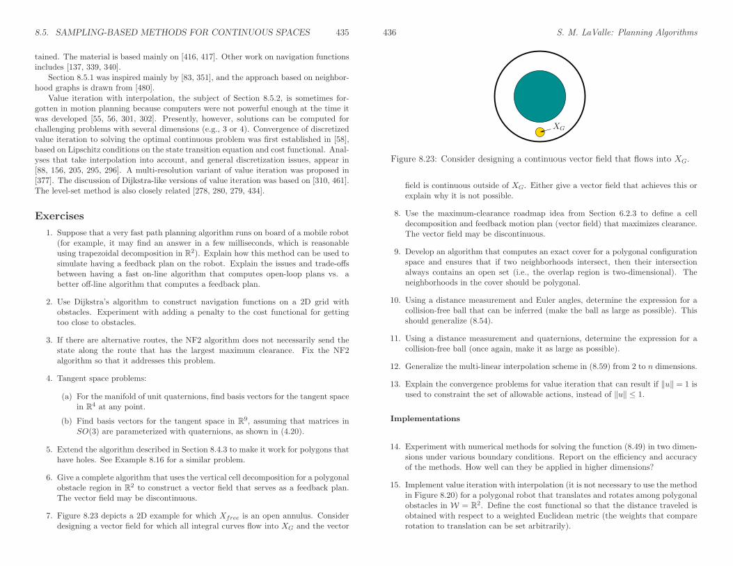
8.5. SAMPLING-BASED METHODS FOR CONTINUOUS SPACES 435
tained. The material is based mainly on [416, 417]. Other work on navigation functionsincludes [137, 339, 340].
Section 8.5.1 was inspired mainly by [83, 351], and the approach based on neighbor-hood graphs is drawn from [480].
Value iteration with interpolation, the subject of Section 8.5.2, is sometimes for-gotten in motion planning because computers were not powerful enough at the time itwas developed [55, 56, 301, 302]. Presently, however, solutions can be computed forchallenging problems with several dimensions (e.g., 3 or 4). Convergence of discretizedvalue iteration to solving the optimal continuous problem was first established in [58],based on Lipschitz conditions on the state transition equation and cost functional. Anal-yses that take interpolation into account, and general discretization issues, appear in[88, 156, 205, 295, 296]. A multi-resolution variant of value iteration was proposed in[377]. The discussion of Dijkstra-like versions of value iteration was based on [310, 461].The level-set method is also closely related [278, 280, 279, 434].
Exercises
1. Suppose that a very fast path planning algorithm runs on board of a mobile robot(for example, it may find an answer in a few milliseconds, which is reasonableusing trapezoidal decomposition in R2). Explain how this method can be used tosimulate having a feedback plan on the robot. Explain the issues and trade-offsbetween having a fast on-line algorithm that computes open-loop plans vs. abetter off-line algorithm that computes a feedback plan.
2. Use Dijkstra’s algorithm to construct navigation functions on a 2D grid withobstacles. Experiment with adding a penalty to the cost functional for gettingtoo close to obstacles.
3. If there are alternative routes, the NF2 algorithm does not necessarily send thestate along the route that has the largest maximum clearance. Fix the NF2algorithm so that it addresses this problem.
4. Tangent space problems:
(a) For the manifold of unit quaternions, find basis vectors for the tangent spacein R4 at any point.
(b) Find basis vectors for the tangent space in R9, assuming that matrices inSO(3) are parameterized with quaternions, as shown in (4.20).
5. Extend the algorithm described in Section 8.4.3 to make it work for polygons thathave holes. See Example 8.16 for a similar problem.
6. Give a complete algorithm that uses the vertical cell decomposition for a polygonalobstacle region in R2 to construct a vector field that serves as a feedback plan.The vector field may be discontinuous.
7. Figure 8.23 depicts a 2D example for which Xfree is an open annulus. Considerdesigning a vector field for which all integral curves flow into XG and the vector
436 S. M. LaValle: Planning Algorithms
XG
Figure 8.23: Consider designing a continuous vector field that flows into XG.
field is continuous outside of XG. Either give a vector field that achieves this orexplain why it is not possible.
8. Use the maximum-clearance roadmap idea from Section 6.2.3 to define a celldecomposition and feedback motion plan (vector field) that maximizes clearance.The vector field may be discontinuous.
9. Develop an algorithm that computes an exact cover for a polygonal configurationspace and ensures that if two neighborhoods intersect, then their intersectionalways contains an open set (i.e., the overlap region is two-dimensional). Theneighborhoods in the cover should be polygonal.
10. Using a distance measurement and Euler angles, determine the expression for acollision-free ball that can be inferred (make the ball as large as possible). Thisshould generalize (8.54).
11. Using a distance measurement and quaternions, determine the expression for acollision-free ball (once again, make it as large as possible).
12. Generalize the multi-linear interpolation scheme in (8.59) from 2 to n dimensions.
13. Explain the convergence problems for value iteration that can result if ‖u‖ = 1 isused to constraint the set of allowable actions, instead of ‖u‖ ≤ 1.
Implementations
14. Experiment with numerical methods for solving the function (8.49) in two dimen-sions under various boundary conditions. Report on the efficiency and accuracyof the methods. How well can they be applied in higher dimensions?
15. Implement value iteration with interpolation (it is not necessary to use the methodin Figure 8.20) for a polygonal robot that translates and rotates among polygonalobstacles in W = R2. Define the cost functional so that the distance traveled isobtained with respect to a weighted Euclidean metric (the weights that comparerotation to translation can be set arbitrarily).

8.5. SAMPLING-BASED METHODS FOR CONTINUOUS SPACES i
16. Evaluate the efficiency of the interpolation method shown in Figure 8.20 appliedto multi-linear interpolation given by generalizing (8.59) as in Exercise 12. Youdo not need to implement the full value iteration approach (alternatively, thiscould be done, which provides a better comparison of the overall performance).
17. Implement the method of Section 8.4.2 of computing vector fields on a triangula-tion. For given input polygons, have your program draw a needle diagram of thecomputed vector field. Determine how fast the vector field can be recomputed asthe goal changes.
18. Optimal navigation function problems:
(a) Implement the algorithm illustrated in Figure 8.13. Show the level sets ofthe optimal cost-to-go function.
(b) Extend the algorithm and implementation to the case in which there arepolygonal holes in Xfree.
19. Adapt value iteration with interpolation so that a point robot moving in the planecan keep track of a predictable moving point called a target. The cost functionalshould cause a small penalty to be added if the target is not visible. Optimizingthis should minimize the amount of time that the target is not visible. Assumethat the initial configuration of the robot is given. Compute optimal feedbackplans for the robot.
20. Try to experimentally construct navigation functions by adding potential func-tions that repel the state away from obstacles and attract the state toward xG.For simplicity, you may assume that X = R2 and the obstacles are discs. Startwith a single disc and then gradually construct more complicated obstacle re-gions. How difficult is it to ensure that the resulting potential function has nolocal minima outside of xG?
ii S. M. LaValle: Planning Algorithms

Bibliography
[1] D. Aarno, D. Kragic, and H. I. Christensen. Artificial potential biased prob-abilistic roadmap method. In Proceedings IEEE International Conferenceon Robotics & Automation, 2004.
[2] R. Abraham, J. Marsden, and T. Ratiu. Manifolds, Tensor Analysis, andApplications, 2nd Ed. Springer-Verlag, Berlin, 1988.
[3] A. Abrams and R. Ghrist. Finding topology in a factory: Configurationspaces. The American Mathematics Monthly, 109:140–150, February 2002.
[4] E. U. Acar and H. Choset. Complete sensor-based coverage with extended-range detectors: A hierarchical decomposition in terms of critical points andVoronoi diagrams. In Proceedings IEEE/RSJ International Conference onIntelligent Robots and Systems, 2001.
[5] E. U. Acar and H. Choset. Robust sensor-based coverage of unstructuredenvironments. In Proceedings IEEE/RSJ International Conference on In-telligent Robots and Systems, 2001.
[6] C. C. Adams. The Knot Book: An Elementary Introduction to the Mathe-matical Theory of Knots. W. H. Freeman, New York, 1994.
[7] P. Agarwal, M. de Berg, D. Halperin, and M. Sharir. Efficient generationof k-directional assembly sequences. In ACM Symposium on Discrete Algo-rithms, pages 122–131, 1996.
[8] P. K. Agarwal, N. Amenta, B. Aronov, and M. Sharir. Largest placementsand motion planning of a convex polygon. In J.-P. Laumond and M. Over-mars, editors, Robotics: The Algorithmic Perspective. A.K. Peters, Welles-ley, MA, 1996.
[9] P. K. Agarwal, B. Aronov, and M. Sharir. Motion planning for a convexpolygon in a polygonal environment. Discrete and Computational Geometry,22:201–221, 1999.
[10] S. Akella and S. Hutchinson. Coordinating the motions of multiple robotswith specified trajectories. In Proceedings IEEE International Conferenceon Robotics & Automation, pages 624–631, 2002.
iii
iv BIBLIOGRAPHY
[11] R. Alami, J.-P. Laumond, and T. Simeon. Two manipulation planningalgorithms. In J.-P. Laumond and M. Overmars, editors, Algorithms forRobotic Motion and Manipulation. A.K. Peters, Wellesley, MA, 1997.
[12] R. Alami, T. Simeon, and J.-P. Laumond. A geometrical approach toplanning manipulation tasks. In Proceedings International Symposium onRobotics Research, pages 113–119, 1989.
[13] G. Allgower and K. Georg. Numerical Continuation Methods. Springer-Verlag, Berlin, 1990.
[14] H. Alt, R. Fleischer, M. Kaufmann, K. Mehlhorn, S. Naher, S. Schirra, andC. Uhrig. Approximate motion planning and the complexity of the boundaryof the union of simple geometric figures. In Proceedings ACM Symposiumon Computational Geometry, pages 281–289, 1990.
[15] N. M. Amato, O. B. Bayazit, L. K. Dale, C. Jones, and D. Vallejo. Choosinggood distance metrics and local planners for probabilistic roadmap methods.In Proceedings IEEE International Conference on Robotics & Automation,pages 630–637, 1998.
[16] N. M. Amato, O. B. Bayazit, L. K. Dale, C. Jones, and D. Vallejo. OBPRM:An obstacle-based PRM for 3D workspaces. In Proceedings Workshop onAlgorithmic Foundations of Robotics, pages 155–168, 1998.
[17] N. M. Amato, O. B. Bayazit, L. K. Dale, C. Jones, and D. Vallejo. Choosinggood distance metrics and local planners for probabilistic roadmap methods.IEEE Transactions on Robotics & Automation, 16(4):442–447, Aug 2000.
[18] N. M. Amato, K. A. Dill, and G. Song. Using motion planning to map pro-tein folding landscapes and analyze folding kinetics of known native struc-tures. In Proceedings 6th ACM International Conference on ComputationalMolecular Biology (RECOMB), pages 2–11, 2002.
[19] N. M. Amato and G. Song. Using motion planning to study protein foldingpathways. Journal of Computational Biology, 9(2):149–168, 2002.
[20] N. M. Amato and Y. Wu. A randomized roadmap method for path andmanipulation planning. In Proceedings IEEE International Conference onRobotics & Automation, pages 113–120, 1996.
[21] F. Ancona and A. Bressan. Patchy vector fields and asymptotic stabilization.ESAIM-Control, Optimisation and Calculus of Variations, 4:445–471, 1999.
[22] B. D. Anderson and J. B. Moore. Optimal Control: Linear-Quadratic Meth-ods. Prentice-Hall, Englewood Cliffs, NJ, 1990.
BIBLIOGRAPHY v
[23] J. Angeles. Spatial Kinematic Chains. Analysis, Synthesis, and Optimisa-tion. Springer-Verlag, Berlin, 1982.
[24] J. Angeles. Fundamentals of Robotic Mechanical Systems: Theory, Methods,and Algorithms. Springer-Verlag, Berlin, 2003.
[25] E. Anshelevich, S. Owens, F. Lamiraux, and L. E. Kavraki. Deformablevolumes in path planning applications. In Proceedings IEEE InternationalConference on Robotics & Automation, pages 2290–2295, 2000.
[26] M. Apaydin, D. Brutlag, C. Guestrin, D. Hsu J.-C. Latombe, and C. Varm.Stochastic roadmap simulation: An efficient representation and algorithmfor analyzing molecular motion. Journal of Computational Biology, 10:257–281, 2003.
[27] M. D. Ardema and J. M. Skowronski. Dynamic game applied to coordinationcontrol of two arm robotic system. In R. P. Hamalainen and H. K. Ehtamo,editors, Differential Games – Developments in Modelling and Computation,pages 118–130. Springer-Verlag, Berlin, 1991.
[28] E. M. Arkin and R. Hassin. Approximation algorithms for the geometriccovering traveling salesman problem. Discrete Applied Mathematics, 55:194–218, 1994.
[29] B. Armstrong, O. Khatib, and J. Burdick. The explicit dynamic model andinertial parameters of the Puma 560 arm. In Proceedings IEEE InternationalConference on Systems, Man, & Cyberetics, pages 510–518, 1986.
[30] M. A. Armstrong. Basic Topology. Springer-Verlag, New York, 1983.
[31] D. S. Arnon. Geometric reasoning with logic and algebra. Artificial Intelli-gence Journal, 37(1-3):37–60, 1988.
[32] B. Aronov, M. de Berg, A. F. van der Stappen, P. Svestka, and J. Vleugels.Motion planning for multiple robots. Discrete and Computational Geometry,22:505–525, 1999.
[33] B. Aronov and M. Sharir. On translational motion planning of a convexpolyhedron in 3-space. SIAM Journal on Computing, 26(6):1875–1803, De-cember 1997.
[34] D. K. Arrowsmith and C. M. Place. Dynamical Systems: Differential Equa-tions, Maps, and Chaotic Behaviour. Chapman & Hall/CRC, New York,1992.
[35] S. Arya and D. M. Mount. Algorithms for fast vector quantization. In IEEEData Compression Conference, pages 381–390, March 1993.
vi BIBLIOGRAPHY
[36] S. Arya and D. M. Mount. Approximate nearest neighbor queries in fixeddimensions. In Proceedings ACM-SIAM Symposium on Discrete Algorithms,pages 271–280, 1993.
[37] S. Arya, D. M. Mount, N. S. Netanyahu, R. Silverman, and A. Y. Wu. Anoptimal algorithm for approximate nearest neighbor searching. Journal ofthe ACM, 45:891–923, 1998.
[38] A. Atramentov and S. M. LaValle. Efficient nearest neighbor searching formotion planning. In Proceedings IEEE International Conference on Roboticsand Automation, pages 632–637, 2002.
[39] J.-P. Aubin and A. Cellina. Differential Inclusions. Springer-Verlag, Berlin,1984.
[40] F. Aurenhammer. Voronoi diagrams – A survey of a fundamental geometricstructure. ACM Computing Surveys, 23:345–405, 1991.
[41] F. Avnaim, J.-D. Boissonnat, and B. Faverjon. A practical exact plan-ning algorithm for polygonal objects amidst polygonal obstacles. In Pro-ceedings IEEE International Conference on Robotics & Automation, pages1656–1660, 1988.
[42] J. Banon. Implementation and extension of the ladder algorithm. In Pro-ceedings IEEE International Conference on Robotics & Automation, pages1548–1553, 1990.
[43] B. Baginski. The Z3 method for fast path planning in dynamic environ-ments. In Proceedings IASTED Conference on Applications of Control andRobotics, pages 47–52, 1996.
[44] B. Baginski. Motion Planning for Manipulators with Many Degrees of Free-dom – The BB-Method. PhD thesis, Technical University of Munich, 1998.
[45] A. Baker. Matrix Groups. Springer-Verlag, Berlin, 2002.
[46] D. J. Balkcom and M. T. Mason. Introducing robotic origami folding.In Proceedings IEEE International Conference on Robotics & Automation,2004.
[47] J. Barraquand, L. Kavraki, J.-C. Latombe, T.-Y. Li, R. Motwani, andP. Raghavan. A random sampling scheme for robot path planning. InG. Giralt and G. Hirzinger, editors, Proceedings International Symposiumon Robotics Research, pages 249–264. Springer-Verlag, New York, 1996.
[48] J. Barraquand and J.-C. Latombe. A Monte-Carlo algorithm for path plan-ning with many degrees of freedom. In Proceedings IEEE InternationalConference on Robotics & Automation, pages 1712–1717, 1990.

BIBLIOGRAPHY vii
[49] J. Barraquand and J.-C. Latombe. Nonholonomic multibody mobile robots:Controllability and motion planning in the presence of obstacles. In Pro-ceedings IEEE International Conference on Robotics & Automation, pages2328–2335, 1991.
[50] J. Barraquand and J.-C. Latombe. Robot motion planning: A dis-tributed representation approach. International Journal of Robotics Re-search, 10(6):628–649, December 1991.
[51] J. Basch, L. J. Guibas, D. Hsu, and A. T. Nguyen. Disconnection proofs formotion planning. In Proceedings IEEE International Conference on Robotics& Automation, pages 1765–1772, 2001.
[52] S. Basu, R. Pollack, and M. F. Roy. Computing roadmaps of semi-algebraicsets on a variety. Journal of the American Society of Mathematics, 3(1):55–82, 1999.
[53] S. Basu, R. Pollack, and M.-F. Roy. Algorithms in Real Algebraic Geometry.Springer-Verlag, Berlin, 2003.
[54] K. E. Bekris, B. Y. Chen, A. Ladd, E. Plaku, and L. E. Kavraki. Multi-ple query probabilistic roadmap planning using single query primitives. InProceedings IEEE/RSJ International Conference on Intelligent Robots andSystems, 2003.
[55] R. E. Bellman. Dynamic Programming. Princeton University Press, Prince-ton, NJ, 1957.
[56] R. E. Bellman and S. E. Dreyfus. Applied Dynamic Programming. PrincetonUniversity Press, Princeton, NJ, 1962.
[57] M. Bern. Triangulations and mesh generation. In J. E. Goodman andJ. O’Rourke, editors, Handbook of Discrete and Computational Geometry,2nd Ed., pages 563–582. Chapman and Hall/CRC Press, New York, 2004.
[58] D. P. Bertsekas. Convergence in discretization procedures in dynamic pro-gramming. IEEE Transactions on Automatic Control, 20(3):415–419, June1975.
[59] D. P. Bertsekas. Dynamic Programming and Optimal Control, Vol. II, 2ndEd. Athena Scientific, Belmont, MA, 2001.
[60] D. P. Bertsekas and J. N. Tsitsiklis. Neuro-Dynamic Programming. AthenaScientific, Belmont, MA, 1996.
[61] A. Beygelzimer, S. M. Kakade, and J. Langford. Cover treesfor nearest neighbor. University of Pennsylvania, Available fromhttp://www.cis.upenn.edu/∼skakade/papers/ml/cover tree.pdf, 2005.
viii BIBLIOGRAPHY
[62] R. L. Bishop and S. I. Goldberg. Tensor Analysis on Manifolds. Dover, NewYork, 1980.
[63] H. S. Black. Stabilized feedback amplifiers. Bell Systems Technical Journal,13:1–18, 1934.
[64] A. Blum, S. Chawla, D. Karger, T. Lane, A. Meyerson, and M. Minkoff.Approximation algorithms for orienteering and discounted-reward TSP. InProceedings IEEE Symposium on Foundations of Computer Science, 2003.
[65] L. Blum, F. Cucker, and M. Schub abd S. Smale. Complexity and RealComputation. Springer-Verlag, Berlin, 1998.
[66] H. Bode. Feedback: The history of an idea. In R. Bellman and R. Kalaba,editors, Selected Papers on Mathematical Trends in Control Theory, pages106–123. Dover, New York, 1969.
[67] R. Bohlin. Path planning in practice; lazy evaluation on a multi-resolutiongrid. In Proceedings IEEE/RSJ International Conference on IntelligentRobots and Systems, 2001.
[68] R. Bohlin. Robot Path Planning. PhD thesis, Chalmers University, Gothen-burg, Sweden, 2002.
[69] R. Bohlin and L. Kavraki. Path planning using Lazy PRM. In ProceedingsIEEE International Conference on Robotics & Automation, 2000.
[70] K.-F. Bohringer, B. R. Donald, and N. C. MacDonald. Upper and lowerbounds for programmable vector fields with applications to MEMS and vi-bratory plate parts feeders. In J.-P. Laumond and M. Overmars, editors,Algorithms for Robotic Motion and Manipulation. A.K. Peters, Wellesley,MA, 1997.
[71] J.-D. Boissonnat and M. Yvinec. Algorithmic Geometry. Cambridge Uni-versity Press, Cambridge, U.K., 1998.
[72] V. Boor, M. H. Overmars, and A. F. van der Stappen. The Gaussian sam-pling strategy for probabilistic roadmap planners. In Proceedings IEEE In-ternational Conference on Robotics & Automation, pages 1018–1023, 1999.
[73] W. M. Boothby. An Introduction to Differentiable Manifolds and Rieman-nian Geometry. Revised 2nd Ed. Academic, New York, 2003.
[74] M. S. Branicky, V. S. Borkar, and S. K. Mitter. A unified framework forhybrid control: Model and optimal control theory. IEEE Transactions onAutomatic Control, 43(1):31–45, 1998.

BIBLIOGRAPHY ix
[75] M. S. Branicky, M. M. Curtiss, J. Levine, and S. Morgan. RRTs for non-linear, discrete, and hybrid planning and control. In Proceedings IEEEConference Decision & Control, 2003.
[76] M. Bridson and A. Haefliger. Metric Spaces of Non-Positive Curvature.Springer-Verlag, Berlin, 1999.
[77] R. A. Brooks and T. Lozano-Perez. A subdivision algorithm in configurationspace for findpath with rotation. IEEE Transactions on Systems, Man, &Cybernetics, SMC-15(2):224–233, 1985.
[78] J. Bruce and M. Veloso. Real-time randomized path planning for robot nav-igation. In Proceedings IEEE/RSJ International Conference on IntelligentRobots and Systems, 2002.
[79] A. E. Bryson and Y.-C. Ho. Applied Optimal Control. Hemisphere Publish-ing Corp., New York, 1975.
[80] S. J. Buckley. Fast motion planning for multiple moving robots. In Pro-ceedings IEEE International Conference on Robotics & Automation, pages322–326, 1989.
[81] J. W. Burdick. Kinematic Analysis and Design of Redundant Manipulators.PhD thesis, Stanford University, Stanford, CA, 1988.
[82] B. Burns and O. Brock. Sampling-based motion planning using predictivemodels. In Proceedings IEEE International Conference on Robotics & Au-tomation, 2005.
[83] R. R. Burridge, A. A. Rizzi, and D. E. Koditschek. Sequential compositionof dynamically dexterous robot behaviors. International Journal of RoboticsResearch, 18(6):534–555, 1999.
[84] Z. J. Butler, A. A. Rizzi, and R. L. Hollis. Contact sensor-based coverage ofrectilinear environments. In IEEE Symposium on Intelligent Control, 1999.
[85] Z. J. Butler and D. Rus. Distributed motion planning for modular robotswith unit-compressible modules. International Journal of Robotics Research,22(9):699–716, 2003.
[86] S. Cambon, F. Gravot, and R. Alami. A robot task planner and mergessymbolic and geometric reasoning. In Proceedings European Conference onArtificial Intelligence, 2004.
[87] S. Cameron. A comparison of two fast algorithms for computing the distancebetween convex polyhedra. IEEE Transactions on Robotics & Automation,13(6):915–920, December 1997.
x BIBLIOGRAPHY
[88] F. Camilli and M. Falcone. Approximation of optimal control problems withstate constraints: Estimates and applications. In B. S. Mordukhovich andH. J. Sussmann, editors, Nonsmooth Analysis and Geometric Methods inDeterministic Optimal Control, pages 23–57. Springer-Verlag, Berlin, 1996.Mathematics and its Applications, Vol. 78.
[89] J. Canny. Constructing roadmaps of semi-algebraic sets I. Artificial Intelli-gence Journal, 37:203–222, 1988.
[90] J. Canny. Computing roadmaps of general semi-algebraic sets. The Com-puter Journal, 36(5):504–514, 1993.
[91] J. Canny and J. Reif. New lower bound techniques for robot motion planningproblems. In Proceedings IEEE Symposium on Foundations of ComputerScience, pages 49–60, 1987.
[92] J. F. Canny. The Complexity of Robot Motion Planning. MIT Press, Cam-bridge, MA, 1988.
[93] J. F. Canny and M. Lin. An opportunistic global path planner. Algorithmica,10:102–120, 1993.
[94] S. Carpin and E. Pagello. On parallel RRTs for multi-robot systems. In Pro-ceedings 8th Conference of the Italian Association for Artificial Intelligence,pages 834–841, 2002.
[95] S. Carpin and G. Pillonetto. Merging the adaptive random walks plannerwith the randomized potential field planner. In Proceedings IEEE Interna-tional Workshop on Robot Motion and Control, pages 151–156, 2005.
[96] S. Carpin and G. Pillonetto. Robot motion planning using adaptive randomwalks. IEEE Transactions on Robotics & Automation, 21(1):129–136, 2005.
[97] A. Casal. Reconfiguration Planning for Modular Self-Reconfigurable Robots.PhD thesis, Stanford University, Stanford, CA, 2002.
[98] S. Caselli and M. Reggiani. ERPP: An experience-based randomized pathplanner. In Proceedings IEEE International Conference on Robotics & Au-tomation, 2000.
[99] D. Challou, D. Boley, M. Gini, and V. Kumar. A parallel formulation ofinformed randomized search for robot motion planning problems. In Pro-ceedings IEEE International Conference on Robotics & Automation, pages709–714, 1995.
[100] H. Chang and T. Y. Li. Assembly maintainability study with motion plan-ning. In Proceedings IEEE International Conference on Robotics & Automa-tion, pages 1012–1019, 1995.
BIBLIOGRAPHY xi
[101] S. Charentus. Modeling and Control of a Robot Manipulator Composed ofSeveral Stewart Platforms. PhD thesis, Universite Paul Sabatier, Toulouse,France, 1990. In French.
[102] S. Chawla. Graph Algorithms for Planning and Partitioning. PhD thesis,Carnegie Mellon University, Pittsburgh, PA, June 2005.
[103] B. Chazelle. Approximation and decomposition of shapes. In J. T. Schwartzand C. K. Yap, editors, Algorithmic and Geometric Aspects of Robotics,pages 145–185. Lawrence Erlbaum Associates, Hillsdale, NJ, 1987.
[104] B. Chazelle. Triangulating a simple polygon in linear time. Discrete andComputational Geometry, 6(5):485–524, 1991.
[105] B. Chazelle. The Discrepancy Method. Cambridge University Press, Cam-bridge, U.K., 2000.
[106] C.-T. Chen. Linear System Theory and Design. Holt, Rinehart, and Win-ston, New York, 1984.
[107] P. C. Chen and Y. K. Hwang. SANDROS: A motion planner with perfor-mance proportional to task difficulty. In Proceedings IEEE InternationalConference on Robotics & Automation, pages 2346–2353, 1992.
[108] P. C. Chen and Y. K. Hwang. SANDROS: A dynamic search graph algo-rithm for motion planning. IEEE Transactions on Robotics & Automation,14(3):390–403, 1998.
[109] P. Cheng and S. M. LaValle. Resolution complete rapidly-exploring ran-dom trees. In Proceedings IEEE International Conference on Robotics andAutomation, pages 267–272, 2002.
[110] L. P. Chew and K. Kedem. A convex polygon among polygonal obstacles:Placement and high-clearance motion. Computational Geometry: Theoryand Applications, 3:59–89, 1993.
[111] D. Chibisov, E. W. Mayr, and S. Pankratov. Spatial planning and geomet-ric optimization: Combining configuration space and energy methods. InH. Hong and D. Wang, editors, Automated Deduction in Geometry - ADG2004. Springer-Verlag, Berlin, 2006.
[112] G. Chirikjian, A. Pamecha, and I. Ebert-Uphoff. Evaluating efficiency of self-reconfiguration in a class of modular robots. Journal of Robotic Systems,13(5):717–338, 1996.
[113] G. S. Chirikjian and A. B. Kyatkin. Engineering Applications of Noncom-mutative Harmonic Analysis. CRC Press, Boca Raton, FL, 2001.
xii BIBLIOGRAPHY
[114] H. Chitsaz, J. M. O’Kane, and S. M. LaValle. Pareto-optimal coordinationof two translating polygonal robots on an acyclic roadmap. In ProceedingsIEEE International Conference on Robotics and Automation, 2004.
[115] J. Choi, J. Sellen, and C. K. Yap. Precision-sensitive Euclidean shortest pathin 3-space. In Proceedings ACM Symposium on Computational Geometry,pages 350–359, 1995.
[116] H. Choset. Coverage of known spaces: The boustrophedon cellular decom-position. Autonomous Robots, 9:247–253, 2000.
[117] H. Choset. Coverage for robotics – A survey of recent results. Annals ofMathematics and Artificial Intelligence, 31:113–126, 2001.
[118] H. Choset, K. M. Lynch, S. Hutchinson, G. Kantor, W. Burgard, L. E.Kavraki, and S. Thrun. Principles of Robot Motion: Theory, Algorithms,and Implementations. MIT Press, Cambridge, MA, 2005.
[119] H. Choset and P. Pignon. Cover path planning: The boustrophedron de-composition. In Proceedings International Conference on Field and ServiceRobotics, Canberra, Australia, December 1997.
[120] P. Choudhury and K. Lynch. Trajectory planning for second-order underac-tuated mechanical systems in presence of obstacles. In Proceedings Workshopon Algorithmic Foundations of Robotics, 2002.
[121] C. M. Clark, S. M. Rock, and J.-C. Latombe. Motion planning for multiplemobile robots using dynamic networks. In Proceedings IEEE InternationalConference on Robotics & Automation, 2003.
[122] D. E. Clark, G. Jones, P. Willett P. W. Kenny, and R. C. Glen. Pharma-cophoric pattern matching in files of three-dimensional chemical structures:Comparison of conformational searching algorithms for flexible searching.Journal Chemical Information and Computational Sciences, 34:197–206,1994.
[123] K. L. Clarkson. Nearest neighbor searching in metric spaces: Ex-perimental results for sb(s). Bell Labs. Available from http://cm.bell-labs.com/who/clarkson/Msb/readme.html, 2003.
[124] G. E. Collins. Quantifier elimination for real closed fields by cylindrical al-gebraic decomposition. In Proceedings Second GI Conference on AutomataTheory and Formal Languages, pages 134–183, Berlin, 1975. Springer-Verlag. Lecture Notes in Computer Science, 33.
[125] G. E. Collins. Quantifier elimination by cylindrical algebraic decomposition–twenty years of progress. In B. F. Caviness and J. R. Johnson, editors,

BIBLIOGRAPHY xiii
Quantifier Elimination and Cylindrical Algebraic Decomposition, pages 8–23. Springer-Verlag, Berlin, 1998.
[126] L. Conlon. Differentiable Manifolds, 2nd Ed. Birkhauser, Boston, MA, 2001.
[127] D. C. Conner, A. A. Rizzi, and H. Choset. Composition of local potentialfunctions for global robot control and navigation. In Proceedings IEEE/RSJInternational Conference on Intelligent Robots and Systems, pages 3546–3551, 2003.
[128] C. Connolly and R. Grupen. The application of harmonic potential functionsto robotics. Journal of Robotic Systems, 10(7):931–946, 1993.
[129] C. I. Connolly. Applications of harmonic functions to robotics. In IEEESymposium on Intelligent Control, pages 498–502, 1992.
[130] C. I. Connolly, J. B. Burns, and R. Weiss. Path planning using Laplace’sequation. In Proceedings IEEE International Conference on Robotics &Automation, pages 2102–2106, May 1990.
[131] J. H. Conway and N. J. A. Sloane. Sphere Packings, Lattices, and Groups.Springer-Verlag, Berlin, 1999.
[132] T. H. Cormen, C. E. Leiserson, R. L. Rivest, and C. Stein. Introduction toAlgorithms (2nd Ed.). MIT Press, Cambridge, MA, 2001.
[133] J. Cortes. Motion Planning Algorithms for General Closed-Chain Mecha-nisms. PhD thesis, Institut National Polytechnique de Toulouse, Toulouse,France, 2003.
[134] J. Cortes, T. Simeon M. Remaud-Simeon, and V. Tran. Geometric algo-rithms for the conformational analysis of long protein loops. Journal ofComputational Chemistry, 25:956–967, 2004.
[135] J. Cortes, T. Simeon, and J.-P. Laumond. A random loop generator for plan-ning the motions of closed kinematic chains using PRM methods. In Pro-ceedings IEEE International Conference on Robotics & Automation, 2002.
[136] M. G. Coutinho. Dynamic Simulations of Multibody Systems. Springer-Verlag, Berlin, 2001.
[137] N. Cowan. Composing navigation functions on Cartesian products of mani-folds with boundary. In Proceedings Workshop on Algorithmic Foundationsof Robotics, Zeist, The Netherlands, July 2004.
[138] D. Cox, J. Little, and D. O’Shea. Ideals, Varieties, and Algorithms.Springer-Verlag, Berlin, 1992.
xiv BIBLIOGRAPHY
[139] H. S. M. Coxeter. Regular Polytopes. Dover, New York, 1973.
[140] J. J. Craig. Introduction to Robotics. Addison-Wesley, Reading, MA, 1989.
[141] J. C. Culberson. Sokoban is PSPACE-complete. In Proceedings Interna-tional Conference on Fun with Algorithms (FUN98), pages 65–76, Waterloo,Ontario, Canada, June 1998. Carleton Scientific.
[142] M. R. Cutkosky. Robotic Grasping and Fine Manipulation. Kluwer, Boston,MA, 1985.
[143] L. K. Dale and N. M. Amato. Probabilistic roadmap methods are embarrass-ingly parallel. In Proceedings IEEE International Conference on Robotics &Automation, 1999.
[144] J. Davenport and J. Heintz. Real quantifier elimination is doubly exponen-tial. Journal of Symbolic Computation, 5:29–35, 1988.
[145] S. Davies. Multidimensional triangulation and interpolation for reinforce-ment learning. In Proceedings Neural Information Processing Systems, 1996.
[146] M. de Berg, M. van Kreveld, M. Overmars, and O. Schwarzkopf. Compu-tational Geometry: Algorithms and Applications, 2nd Ed. Springer-Verlag,Berlin, 2000.
[147] M. J. de Smith. Distance and Path: The Development, Interpretation andApplication of Distance Measurement in Mapping and Modelling. PhD the-sis, University College, University of London, London, 2003.
[148] R. Dial. Algorithm 360: Shortest path forest with topological ordering.Communications of the ACM, 12:632–633, 1969.
[149] D. V. Dimarogonas, M. M. Zavlanos, S. G. Loizou, and K. J. Kyriakopou-los. Decentralized motion control of multiple holonomic agents under inputconstraints. In Proceedings IEEE Conference Decision & Control, 2003.
[150] W. E. Dixon, A. Behal, D. M. Dawson, and S. Nagarkatti. Nonlinear Controlof Engineering Systems: A Lyapunov-Based Approach. Birkhauser, Boston,MA, 2003.
[151] M. P. do Carmo. Riemannian Geometry. Birkhauser, Boston, MA, 1992.
[152] B. R. Donald. Motion planning with six degrees of freedom. TechnicalReport AI-TR-791, Artificial Intelligence Lab., Massachusetts Institute ofTechnology, Cambridge, MA, 1984.
[153] B. R. Donald. A search algorithm for motion planning with six degrees offreedom. Artificial Intelligence Journal, 31:295–353, 1987.
BIBLIOGRAPHY xv
[154] B. R. Donald. A geometric approach to error detection and recovery forrobot motion planning with uncertainty. Artificial Intelligence Journal,37:223–271, 1988.
[155] S. K. Donaldson. Self-dual connections and the topology of smooth 4-manifold. Bulletin of the American Mathematical Society, 8:81–83, 1983.
[156] A. L. Dontchev. Discrete approximations in optimal control. In B. S. Mor-dukhovich and H. J. Sussmann, editors, Nonsmooth Analysis and GeometricMethods in Deterministic Optimal Control, pages 59–80. Springer-Verlag,Berlin, 1996. Mathematics and Its Applications, Vol. 78.
[157] G. E. Dullerud and R. D’Andrea. Distributed control of heterogeneoussystems. IEEE Transactions on Automatic Control, 49(12):2113–2128, 2004.
[158] H. Edelsbrunner. Algorithms in Combinatorial Geometry. Springer-Verlag,Berlin, 1987.
[159] C. Edwards and S. K. Spurgeon. Sliding Mode Control: Theory and Appli-cations. CRC Press, Ann Arbor, MI, 1998.
[160] M. Egerstedt and X. Hu. Formation constrained multi-agent control. IEEETransactions on Robotics & Automation, 17(6):947–951, December 2001.
[161] S. Ehmann and M. C. Lin. Accurate and fast proximity queries betweenpolyhedra using convex surface decomposition. In Proceedings Eurographics,2001.
[162] I. Z. Emiris and B. Mourrain. Computer algebra methods for studyingand computing molecular conformations. Technical report, INRIA, Sophia-Antipolis, France, 1997.
[163] A. G. Erdman, G. N. Sandor, and S. Kota. Mechanism Design: Analysisand Synthesis, 4th Ed., Vol. 1. Prentice Hall, Englewood Cliffs, NJ, 2001.
[164] M. A. Erdmann. Understanding action and sensing by designing action-based sensors. International Journal of Robotics Research, 14(5):483–509,1995.
[165] M. A. Erdmann and T. Lozano-Perez. On multiple moving objects. In Pro-ceedings IEEE International Conference on Robotics & Automation, pages1419–1424, 1986.
[166] M. A. Erdmann and T. Lozano-Perez. On multiple moving objects. Algo-rithmica, 2:477–521, 1987.
[167] M. Farber. Topological complexity of motion planning. Discrete and Com-putational Geometry, 29:211–221, 2003.
xvi BIBLIOGRAPHY
[168] M. Farber, S. Tabachnkov, and S. Yuzvinsky. Topological robotics: Motionplanning in projective spaces. International Mathematical Research Notices,34:1853–1870, 2003.
[169] M. Farber and S. Yuzvinsky. Topological robotics: Subspace arrangementsand collision free motion planning. Technical Report math.AT/0210115,arXiv (on-line), 2004.
[170] B. Faverjon. Obstacle avoidance using an octree in the configuration space ofa manipulator. In Proceedings IEEE International Conference on Robotics& Automation, pages 504–512, 1984.
[171] B. Faverjon. Hierarchical object models for efficient anti-collision algorithms.In Proceedings IEEE International Conference on Robotics & Automation,pages 333–340, 1989.
[172] B. Faverjon and P. Tournassoud. A local based method for path plan-ning of manipulators with a high number of degrees of freedom. In Pro-ceedings IEEE International Conference on Robotics & Automation, pages1152–1159, 1987.
[173] R. Fierro, A. Das, V. Kumar, and J. P. Ostrowski. Hybrid control of forma-tions of robots. In Proceedings IEEE International Conference on Robotics& Automation, pages 157–162, 2001.
[174] A. F. Filippov. Differential equations with discontinuous right-hand sides.American Mathematical Society Translations, Ser. 2, 64:199–231, 1964.
[175] P. W. Finn, D. Halperin, L. E. Kavraki, J.-C. Latombe, R. Motwani, C. Shel-ton, and S. Venkatasubramanian. Geometric manipulation of flexible lig-ands. In M. C. Lin and D. Manocha, editors, Applied Computational Geom-etry, pages 67–78. Springer-Verlag, Berlin, 1996. Lecture Notes in ComputerScience, 1148.
[176] G. F. Fishman. Monte Carlo: Concepts, Algorithms, and Applications.Springer-Verlag, Berlin, 1996.
[177] H. Flordal, M. Fabian, and K. Akesson. Automatic implementation andverification of coordinating PLC-code for robotcells. In Proceedings IFACSymposium of Information Control Problems in Manufacturing, 2004.
[178] G. B. Folland. Real Analysis: Modern Techniques and Their Applications.Wiley, New York, 1984.
[179] M. Foskey, M. Garber, M. Lin, and D. Manocha. A Voronoi-based hybridmotion planner. In Proceedings IEEE/RSJ International Conference onIntelligent Robots and Systems, 2001.
BIBLIOGRAPHY xvii
[180] E. Frazzoli and F. Bullo. Decentralized algorithms for vehicle routing ina stochastic time-varying environment. In Proceedings IEEE ConferenceDecision & Control, pages 3357–3363, 2004.
[181] E. Frazzoli, M. A. Dahleh, and E. Feron. Real-time motion planning for agileautonomous vehicles. AIAA Journal of Guidance and Control, 25(1):116–129, 2002.
[182] E. Freund and H. Hoyer. Path finding in multi robot systems includingobstacle avoidance. International Journal of Robotics Research, 7(1):42–70,February 1988.
[183] J. H. Friedman, J. L. Bentley, and R.A. Finkel. An algorithm for finding bestmatches in logarithmic expected time. ACM Transactions on MathematicalSoftware, 3(3):209–226, September 1977.
[184] K. S. Fu, R. C. Gonzalez, and C. S. G. Lee. Robotics: Control, Sensing,Vision, and Intelligence. McGraw-Hill, New York, 1987.
[185] K. Fujimura and H. Samet. A hierarchical strategy for path planning amongmoving obstacles. Technical Report CAR-TR-237, Center for AutomationResearch, University of Maryland, November 1986.
[186] K. Fujimura and H. Samet. Planning a time-minimal motion among movingobstacles. Algorithmica, 10:41–63, 1993.
[187] Y. Gabriely and E. Rimon. Spanning-tree based coverage of continuousareas by a mobile robot. Technical report, Dept. of Mechanical Engineering,Technion, Israel Institute of Technology, December 1999.
[188] Y. Gabriely and E. Rimon. Spanning-tree based coverage of continuousareas by a mobile robot. In Proceedings IEEE International Conference onRobotics & Automation, pages 1927–1933, 2001.
[189] Y. Gabriely and E. Rimon. Competitive on-line coverage of grid environ-ments by a mobile robot. Computational Geometry: Theory and Applica-tions, 24(3):197–224, April 2003.
[190] J. Gallier. Curves and Surfaces in Geometric Modeling. Morgan Kaufmann,San Francisco, CA, 2000.
[191] R. Geraerts and M. Overmars. Sampling techniques for probabilisticroadmap planners. In Proceedings International Conference on IntelligentAutonomous Systems, 2004.
[192] R. Geraerts and M. H. Overmars. A comparative study of probabilisticroadmap planners. In Proceedings Workshop on Algorithmic Foundations ofRobotics, December 2002.
xviii BIBLIOGRAPHY
[193] M. Ghallab, D. Nau, and P. Traverso. Automated Planning: Theory andPractice. Morgan Kaufman, San Francisco, CA, 2004.
[194] A. K. Ghose, M. E. Logan, A. M. Treasurywala, H. Wang, R. C. Wahl,B. E. Tomczuk, M. R. Gowravaram, E. P. Jaeger, and J. J. Wendoloski.Determination of pharmacophoric geometry for collagenase inhibitors usinga novel computational method and its verification using molecular dynam-ics, NMR, and X-ray crystallography. Journal of the American ChemicalSociety, 117:4671–4682, 1995.
[195] S. K. Ghosh and D. M. Mount. An output sensitive algorithm for computingvisibility graphs. SIAM Journal on Computing, 20:888–910, 1991.
[196] R. Ghrist. Shape complexes for metamorphic robot systems. In ProceedingsWorkshop on Algorithmic Foundations of Robotics, December 2002.
[197] R. Ghrist, J. M. O’Kane, and S. M. LaValle. Computing Pareto Optimal Co-ordinations on Roadmaps. The International Journal of Robotics Research,24(11):997–1010, 2005.
[198] E. G. Gilbert and D. W. Johnson. Distance functions and their applicationto robot path planning in the presence of obstacles. IEEE Transactions onRobotics & Automation, 1(1):21–30, March 1985.
[199] E. G. Gilbert, D. W. Johnson, and S. S. Keerth. A fast procedure forcomputing the distance between complex objects in three-dimensional space.IEEE Journal of Robotics & Automation, RA-4(2):193–203, Apr 1988.
[200] B. Glavina. Solving findpath by combination of goal-directed and random-ized search. In Proceedings IEEE International Conference on Robotics &Automation, pages 1718–1723, May 1990.
[201] B. Glavina. Planning collision free motions for manipulators through a com-bination of goal oriented search and the creation of intermediate randomsubgoals. PhD thesis, Technical University of Munich, 1991. In German.
[202] J. Go, T. Vu, and J. J. Kuffner. Autonomous behaviors for interactivevehicle animations. In Proceedings SIGGRAPH Symposium on ComputerAnimation, 2004.
[203] M. Goldwasser and R. Motwani. Intractability of assembly sequencing: Unitdisks in the plane. In F. Dehne, A. Rau-Chaplin, J.-R. Sack, and R. Tamas-sia, editors, WADS ’97 Algorithms and Data Structures, pages 307–320.Springer-Verlag, Berlin, 1997. Lecture Notes in Computer Science, 1272.
[204] G. H. Golub and C. F. Van Loan. Matrix Computations (3rd ed). JohnsHopkins University Press, Baltimore, MD, 1996.

BIBLIOGRAPHY xix
[205] R. Gonzalez and E. Rofman. On deterministic control problems: An ap-proximation procedure for the optimal cost, parts I, II. SIAM Journal onControl & Optimization, 23:242–285, 1985.
[206] J. E. Goodman and J. O’Rourke (eds). Handbook of Discrete and Com-putational Geometry, 2nd Ed. Chapman and Hall/CRC Press, New York,2004.
[207] S. Gottschalk, M. C. Lin, and D. Manocha. Obbtree: A hierarchical struc-ture for rapid interference detection. In Proceedings ACM SIGGRAPH,1996.
[208] V. E. Gough and S. G. Whitehall. Universal tyre test machine. In Proceed-ings 9th International Technical Congress F.I.S.I.T.A., May 1962.
[209] E. J. Griffith and S. Akella. Coordinating multiple droplets in planar arraydigital microfluidic systems. International Journal of Robotics Research,24(11):933–949, 2005.
[210] R. Grossman, A. Nerode, A. Ravn, and H. Rischel (eds). Hybrid Systems.Springer-Verlag, Berlin, 1993.
[211] L. Guibas and R. Seidel. Computing convolution by reciprocal search. InProceedings ACM Symposium on Computational Geometry, pages 90–99,1986.
[212] L. J. Guibas, D. Hsu, and L. Zhang. H-Walk: Hierarchical distance com-putation for moving convex bodies. In Proceedings ACM Symposium onComputational Geometry, pages 265–273, 1999.
[213] K. Gupta and Z. Guo. Motion planning with many degrees of freedom:Sequential search with backtracking. IEEE Transactions on Robotics &Automation, 6(11):897–906, 1995.
[214] K. Gupta and X. Zhu. Practical motion planning for many degrees of free-dom: A novel approach within sequential framework. Journal of RoboticSystems, 2(12):105–118, 1995.
[215] P. R. Halmos. Measure Theory. Springer-Verlag, Berlin, 1974.
[216] D. Halperin. Arrangements. In J. E. Goodman and J. O’Rourke, editors,Handbook of Discrete and Computational Geometry, 2nd Ed., pages 529–562. Chapman and Hall/CRC Press, New York, 2004.
[217] D. Halperin, J.-C. Latombe, and R. H. Wilson. A general framework forassembly planning: the motion space approach. In Proceedings ACM Sym-posium on Computational Geometry, pages 9–18, 1998.
xx BIBLIOGRAPHY
[218] D. Halperin and M. Sharir. A near-quadratic algorithm for planning the mo-tion of a polygon in a polygonal environment. Discrete and ComputationalGeometry, 16:121–134, 1996.
[219] D. Halperin and R. Wilson. Assembly partitioning along simple paths: thecase of multiple translations. In Proceedings IEEE International Conferenceon Robotics & Automation, pages 1585–1592, 1995.
[220] J. H. Halton. On the efficiency of certain quasi-random sequences of pointsin evaluating multi-dimensional integrals. Numerische Mathematik, 2:84–90,1960.
[221] J. M. Hammersley. Monte-Carlo methods for solving multivariable problems.Annals of the New York Academy of Science, 86:844–874, 1960.
[222] L. Han and N. M. Amato. A kinematics-based probabilistic roadmap methodfor closed chain systems. In B. R. Donald, K. M. Lynch, and D. Rus, editors,Algorithmic and Computational Robotics: New Directions, pages 233–246.A.K. Peters, Wellesley, MA, 2001.
[223] R. S. Hartenberg and J. Denavit. A kinematic notation for lower pair mech-anisms based on matrices. Journal of Applied Mechanics, 77:215–221, 1955.
[224] R. S. Hartenberg and J. Denavit. Kinematic Synthesis of Linkages. McGraw-Hill, New York, 1964.
[225] R. Hartshorne. Algebraic Geometry. Springer-Verlag, Berlin, 1977.
[226] A. Hatcher. Algebraic Topology. Cambridge Uni-versity Press, Cambridge, U.K., 2002. Available athttp://www.math.cornell.edu/∼hatcher/AT/ATpage.html.
[227] J. Hershberger and S. Suri. Efficient computation of Euclidean shortestpaths in the plane. In Proceedings IEEE Symposium on Foundations ofComputer Science, pages 508–517, 1995.
[228] S. Hert, S. Tiwari, and V. Lumelsky. A terrain-covering algorithm for anAUV. Autonomous Robots, 3:91–119, 1996.
[229] F. J. Hickernell. Lattice rules: How well do they measure up? In P. Bickel,editor, Random and Quasi-Random Point Sets, pages 109–166. Springer-Verlag, Berlin, 1998.
[230] F. J. Hickernell, H. S. Hong, P. L’Ecuyer, and C. Lemieux. Extensible latticesequences for quasi-monte carlo quadrature. SIAM Journal on ScientificComputing, 22:1117–1138, 2000.
[231] M. W. Hirsch. Differential Topology. Springer-Verlag, Berlin, 1994.

BIBLIOGRAPHY xxi
[232] J. G. Hocking and G. S. Young. Topology. Dover, New York, 1988.
[233] R. L. Hoffman. Automated assembly in a CSG domain. In ProceedingsIEEE International Conference on Robotics & Automation, pages 210–215,1989.
[234] C. M. Hoffmann. Geometric and Solid Modeling. Morgan Kaufmann, SanFrancisco, CA, 1989.
[235] C. Holleman and L. E. Kavraki. A framework for using the workspace medialaxis in PRM planners. In Proceedings IEEE International Conference onRobotics & Automation, pages 1408–1413, 2000.
[236] L. S. Homem de Mello and A. C. Sanderson. Representations of mechan-ical assembly sequences. IEEE Transactions on Robotics & Automation,7(2):211–227, 1991.
[237] J. Hopcroft, D. Joseph, and S. Whitesides. Movement problems for 2-dimensional linkages. In J .T .Schwartz, M. Sharir, and J. Hopcroft, edi-tors, Planning, Geometry, and Complexity of Robot Motion, pages 282–329.Ablex, Norwood, NJ, 1987.
[238] J. E. Hopcroft, J. T. Schwartz, and M. Sharir. On the complexity of mo-tion planning for multiple independent objects: PSPACE-hardness of the“warehouseman’s problem”. International Journal of Robotics Research,3(4):76–88, 1984.
[239] J. E. Hopcroft, J. D. Ullman, and R. Motwani. Introduction to AutomataTheory, Languages, and Computation. Addison-Wesley, Reading, MA, 2000.
[240] T. Horsch, F. Schwarz, and H. Tolle. Motion planning for many degreesof freedom: Random reflections at C-space obstacles. In Proceedings IEEEInternational Conference on Robotics & Automation, pages 3318–3323, SanDiego, CA, April 1994.
[241] D. Hsu, T. Jiang, J. Reif, and Z. Sun. The bridge test for sampling nar-row passages with probabilistic roadmap planners. In Proceedings IEEEInternational Conference on Robotics & Automation, 2003.
[242] D. Hsu, J.-C. Latombe, and R. Motwani. Path planning in expansive con-figuration spaces. International Journal Computational Geometry & Appli-cations, 4:495–512, 1999.
[243] W. Huang. Optimal line-sweep-based decompositions for coverage algo-rithms. In Proceedings IEEE International Conference on Robotics & Au-tomation, pages 27–32, 2001.
[244] T. W. Hungerford. Algebra. Springer-Verlag, Berlin, 1984.
xxii BIBLIOGRAPHY
[245] Y. K. Hwang and N. Ahuja. Gross motion planning–A survey. ACM Com-puting Surveys, 24(3):219–291, September 1992.
[246] C. Icking, G. Rote, E. Welzl, and C.-K. Yap. Shortest paths for line seg-ments. Algorithmica, 10:182–200, 1992.
[247] P. Indyk. Nearest neighbors in high-dimensional spaces. In J. E. Goodmanand J. O’Rourke, editors, Handbook of Discrete and Computational Geom-etry, 2nd Ed., pages 877–892. Chapman and Hall/CRC Press, New York,2004.
[248] P. Indyk and R. Motwani. Approximate nearest neighbors: Towards remov-ing the curse of dimensionality. In Proceedings ACM Symposium on Theoryof Computing, pages 604–613, 1998.
[249] P. Isto. Constructing probabilistic roadmaps with powerful local planningand path optimization. In Proceedings IEEE/RSJ International Conferenceon Intelligent Robots and Systems, pages 2323–2328, 2002.
[250] H. Jacob, S. Feder, and J. Slotine. Real-time path planning using harmonicpotential functions in dynamic environment. In Proceedings IEEE Interna-tional Conference on Robotics & Automation, pages 874–881, 1997.
[251] Y.-B. Jia. Computation on parametric curves with an application in grasp-ing. International Journal of Robotics Research, 23(7-8):825–855, 2004.
[252] P. Jimenez, F. Thomas, and C. Torras. Collision detection algorithms formotion planning. In J.-P. Laumond, editor, Robot Motion Planning andControl, pages 1–53. Springer-Verlag, Berlin, 1998.
[253] D. Jordan and M. Steiner. Configuration spaces of mechanical linkages.Discrete and Computational Geometry, 22:297–315, 1999.
[254] D. A. Joseph and W. H. Plantiga. On the complexity of reachability and mo-tion planning questions. In Proceedings ACM Symposium on ComputationalGeometry, pages 62–66, 1985.
[255] S. Kagami, J. Kuffner, K. Nishiwaki, and K. Okada M. Inaba. Humanoidarm motion planning using stereo vision and RRT search. In Proceed-ings IEEE/RSJ International Conference on Intelligent Robots and Systems,2003.
[256] D. W. Kahn. Topology: An Introduction to the Point-Set and AlgebraicAreas. Dover, New York, 1995.
[257] M. Kallmann, A. Aubel, T. Abaci, and D. Thalmann. Planning collision-freereaching motions for interactive object manipulation and grasping. Euro-graphics, 22(3), 2003.
BIBLIOGRAPHY xxiii
[258] M. Kallmann and M. Mataric. Motion planning using dynamic roadmaps.In Proceedings IEEE International Conference on Robotics & Automation,2004.
[259] M. H. Kalos and P. A. Whitlock. Monte Carlo Methods. Wiley, New York,1986.
[260] K. Kant and S. W. Zucker. Toward efficient trajectory planning: The path-velocity decomposition. International Journal of Robotics Research, 5(3):72–89, 1986.
[261] L. Kauffman. Knots and Applications. World Scientific, River Edge, NJ,1995.
[262] L. E. Kavraki. Computation of configuration-space obstacles using theFast Fourier Transform. IEEE Transactions on Robotics & Automation,11(3):408–413, 1995.
[263] L. E. Kavraki. Geometry and the discovery of new ligands. In J.-P. Lau-mond and M. H. Overmars, editors, Algorithms for Robotic Motion andManipulation, pages 435–445. A.K. Peters, Wellesley, MA, 1997.
[264] L. E. Kavraki and M. Kolountzakis. Partitioning a planar assembly into twoconnected parts is NP-complete. Information Processing Letters, 55(3):159–165, 1995.
[265] L. E. Kavraki, P. Svestka, J.-C. Latombe, and M. H. Overmars. Probabilisticroadmaps for path planning in high-dimensional configuration spaces. IEEETransactions on Robotics & Automation, 12(4):566–580, June 1996.
[266] Y. Ke and J. O’Rourke. Lower bounds on moving a ladder in two and threedimensions. Discrete and Computational Geometry, 3:197–217, 1988.
[267] K. Kedem, R. Livne, J. Pach, and M. Sharir. On the union of Jordan regionsand collision-free translational motion amidst polygonal obstacles. Discreteand Computational Geometry, 1:59–71, 1986.
[268] J. M. Keil. Polygon decomposition. In J. R. Sack and J. Urrutia, editors,Handbook on Computational Geometry. Elsevier, New York, 2000.
[269] J. F. Kenney and E. S. Keeping. Mathematics of Statistics, Part 2, 2nd ed.Van Nostrand, Princeton, NJ, 1951.
[270] L. Kettner. Designing a data structure for polyhedral surfaces. In Proceed-ings ACM Symposium on Computational Geometry, pages 146–154, 1998.
[271] H. K. Khalil. Nonlinear Systems. Macmillan, New York, 2002.
xxiv BIBLIOGRAPHY
[272] W. Khalil and J. F. Kleinfinger. A new geometric notation for openand closed-loop robots. In Proceedings IEEE International Conference onRobotics & Automation, volume 3, pages 1174–1179, 1986.
[273] O. Khatib. Commande dynamique dans l’espace operational des robots ma-nipulateurs en presence d’obstacles. PhD thesis, Ecole Nationale de la Statis-tique et de l’Administration Economique, France, 1980.
[274] O. Khatib. Real-time obstacle avoidance for manipulators and mobilerobots. International Journal of Robotics Research, 5(1):90–98, 1986.
[275] J. Kim and J. P. Ostrowski. Motion planning of aerial robot using rapidly-exploring random trees with dynamic constraints. In Proceedings IEEEInternational Conference on Robotics & Automation, 2003.
[276] J.-O. Kim and P. Khosla. Real-time obstacle avoidance using harmonic po-tential functions. Technical report, Carnegie Mellon University, Pittsburgh,PA, 1990.
[277] J. T. Kimbrell. Kinematic Analysis and Synthesis. McGraw-Hill, New York,1991.
[278] R. Kimmel, N. Kiryati, and A. M. Bruckstein. Multivalued distance mapsfor motion planning on surfaces with moving obstacles. IEEE Transactionson Robotics & Automation, 14(3):427–435, June 1998.
[279] R. Kimmel and J. Sethian. Computing geodesic paths on manifolds. Pro-ceedings of the National Academy of Sciences, USA, 95(15):8431–8435, 1998.
[280] R. Kimmel and J. Sethian. Optimal algorithm for shape from shading andpath planning. Journal of Mathematical Imaging and Vision, 14(3):234–244,2001.
[281] C. L. Kinsey. Topology of Surfaces. Springer-Verlag, Berlin, 1993.
[282] J. M. Kleinberg. Two algorithms for nearest-neighbor search in high di-mensions. In Proceedings ACM Symposium on Theory of Computing, pages599–608, May 1997.
[283] D. E. Knuth. The Art of Computer Programming, Volume 2: SeminumericalAlgorithms, 3rd Ed. Addison-Wesley, Reading, MA, 1998.
[284] D. E. Koditschek. Exact robot navigation by means of potential functions:Some topological considerations. In Proceedings IEEE International Con-ference on Robotics & Automation, pages 1–6, 1987.
[285] D. E. Koditschek. An approach to autonomous robot assembly. Robotica,12:137–155, 1994.
BIBLIOGRAPHY xxv
[286] Y. Koga, K. Kondo, J. Kuffner, and J.-C. Latombe. Planning motions withintentions. Proceedings ACM SIGGRAPH, pages 395–408, 1994.
[287] A. N. Kolmogorov and S. V. Fomin. Introductory Real Analysis. Dover,New York, 1975.
[288] V. Koltun. Pianos are not flat: Rigid motion planning in three dimensions.In Proceedings ACM-SIAM Symposium on Discrete Algorithms, 2005.
[289] K. Kondo. Motion planning with six degrees of freedom by multistrate-gic bidirectional heuristic free-space enumeration. IEEE Transactions onRobotics & Automation, 7(3):267–277, 1991.
[290] K. Kotay, D. Rus, M. Vora, and C. McGray. The self-reconfiguring roboticmolecule: Design and control algorithms. In P. K. Agarwal, L. E. Kavraki,and M. T. Mason, editors, Robotics: The Algorithmic Perspective. A.K.Peters, Natick, MA, 1998.
[291] K. Kozlowski, P. Dutkiewicz, and W. Wroblewski. Modeling and Control ofRobots. Wydawnictwo Naukowe PWN, Warsaw, Poland, 2003. In Polish.
[292] J. J. Kuffner. Effective sampling and distance metrics for 3D rigid bodypath planning. In Proceedings IEEE International Conference on Robotics& Automation, 2004.
[293] J. J. Kuffner and S. M. LaValle. An efficient approach to path planningusing balanced bidirectional RRT search. Technical Report CMU-RI-TR-05-34, Robotics Institute, Carnegie Mellon University, Pittsburgh, PA, August2005.
[294] J. B. Kuipers. Quaternions and Rotation Sequences: A Primer with Ap-plications to Orbits, Aerospace, and Virtual Reality. Princeton UniversityPress, Princeton, NJ, 2002.
[295] H. J. Kushner. Numerical methods for continuous control problems in con-tinuous time. SIAM Journal on Control & Optimization, 28:999–1048, 1990.
[296] H. J. Kushner and P. G. Dupuis. Numerical Methods for Stochastic ControlProblems in Continuous Time. Springer-Verlag, Berlin, 1992.
[297] A. Ladd and L. E. Kavraki. Motion planning for knot untangling. In Pro-ceedings Workshop on Algorithmic Foundations of Robotics, Nice, France,December 2002.
[298] A. Ladd and L. E. Kavraki. Fast exploration for robots with dynamics. InProceedings Workshop on Algorithmic Foundations of Robotics, Zeist, TheNetherlands, July 2004.
xxvi BIBLIOGRAPHY
[299] A. Ladd and L. E. Kavraki. Measure theoretic analysis of probabilistic pathplanning. IEEE Transactions on Robotics & Automation, 20(2):229–242,2004.
[300] F. Lamiraux and L. Kavraki. Path planning for elastic plates under ma-nipulation constraints. In Proceedings IEEE International Conference onRobotics & Automation, pages 151–156, 1999.
[301] R. E. Larson. A survey of dynamic programming computational procedures.IEEE Transactions on Automatic Control, 12(6):767–774, December 1967.
[302] R. E. Larson and J. L. Casti. Principles of Dynamic Programming, Part II.Dekker, New York, 1982.
[303] A. Lasota and M. C. Mackey. Chaos, Fractals, and Noise: Stochastic Aspectsof Dynamics, 2nd Ed. Springer-Verlag, Berlin, 1995.
[304] J.-C. Latombe. Robot Motion Planning. Kluwer, Boston, MA, 1991.
[305] J.-C. Latombe. Motion planning: A journey of robots, molecules, digi-tal actors, and other artifacts. International Journal of Robotics Research,18(11):1119–1128, 1999.
[306] S. M. LaValle. Rapidly-exploring random trees: A new tool for path plan-ning. Technical Report 98-11, Computer Science Dept., Iowa State Univer-sity, Oct. 1998.
[307] S. M. LaValle, M. S. Branicky, and S. R. Lindemann. On the relation-ship between classical grid search and probabilistic roadmaps. InternationalJournal of Robotics Research, 23(7/8):673–692, July/August 2004.
[308] S. M. LaValle, P. Finn, L. Kavraki, and J.-C. Latombe. A randomizedkinematics-based approach to pharmacophore-constrained conformationalsearch and database screening. J. Computational Chemistry, 21(9):731–747,2000.
[309] S. M. LaValle and S. A. Hutchinson. Optimal motion planning for multiplerobots having independent goals. IEEE Trans. on Robotics and Automation,14(6):912–925, December 1998.
[310] S. M. LaValle and P. Konkimalla. Algorithms for computing numerical opti-mal feedback motion strategies. International Journal of Robotics Research,20(9):729–752, September 2001.
[311] S. M. LaValle and J. J. Kuffner. Randomized kinodynamic planning. InProceedings IEEE International Conference on Robotics and Automation,pages 473–479, 1999.

BIBLIOGRAPHY xxvii
[312] S. M. LaValle and J. J. Kuffner. Rapidly-exploring random trees: Progressand prospects. In Proceedings Workshop on the Algorithmic Foundations ofRobotics, 2000.
[313] S. M. LaValle and J. J. Kuffner. Randomized kinodynamic planning. Inter-national Journal of Robotics Research, 20(5):378–400, May 2001.
[314] S. M. LaValle and J. J. Kuffner. Rapidly-exploring random trees: Progressand prospects. In B. R. Donald, K. M. Lynch, and D. Rus, editors, Algo-rithmic and Computational Robotics: New Directions, pages 293–308. A KPeters, Wellesley, MA, 2001.
[315] A. R. Leach and I. D. Kuntz. Conformational analysis of flexible ligandsin macromolecular receptor sites. Journal of Computational Chemistry,13(6):730–748, 1992.
[316] D. T. Lee and R. L. Drysdale. Generalization of Voronoi diagrams in theplane. SIAM Journal on Computing, 10:73–87, 1981.
[317] D. H. Lehmer. Mathematical methods in large-scale computing units. InProceedings 2nd Symposium on Large-Scale Digital Computing Machinery,pages 141–146, Cambridge, MA, 1951. Harvard University Press.
[318] J. Lengyel, M. Reichert, B. R. Donald, and D. P. Greenberg. Real-time robotmotion planning using rasterizing computer graphics hardware. ComputerGraphics, 24(4):327–335, August 1990.
[319] D. Leven and M. Sharir. An efficient and simple motion planning algorithmfor a ladder moving in a 2-dimensional space amidst polygonal barriers.Journal of Algorithms, 8:192–215, 1987.
[320] D. Leven and M. Sharir. Planning a purely translational motion for a con-vex object in two-dimensional space using generalized Voronoi diagrams.Discrete and Computational Geometry, 2:9–31, 1987.
[321] P. Leven and S. A. Hutchinson. Real-time path planning in changing envi-ronments. IEEE Transactions on Robotics & Automation, 21(12):999–1030,December 2002.
[322] P. Leven and S. A. Hutchinson. Using manipulability to bias samplingduring the construction of probabilistic roadmaps. IEEE Transactions onRobotics & Automation, 19(6):1020–1026, December 2003.
[323] M. Li and P. Vitanyi. An Introduction to Kolmogorov Complexity and ItsApplications. Springer-Verlag, Berlin, 1997.
xxviii BIBLIOGRAPHY
[324] T.-Y. Li and Y.-C. Shie. An incremental learning approach to motion plan-ning with roadmap management. In Proceedings IEEE International Con-ference on Robotics & Automation, 2002.
[325] D. Liberzon. Switching in Systems and Control. Birkhauser, Boston, MA,2003.
[326] J.-M. Lien, S. L. Thomas, and N. M. Amato. A general framework for sam-pling on the medial axis of the free space. In Proceedings IEEE InternationalConference on Robotics & Automation, 2003.
[327] M. C. Lin and J. F. Canny. Efficient algorithms for incremental distancecomputation. In Proceedings IEEE International Conference on Robotics &Automation, 1991.
[328] M. C. Lin and D. Manocha. Collision and proximity queries. In J. E. Good-man and J. O’Rourke, editors, Handbook of Discrete and ComputationalGeometry, 2nd Ed., pages 787–807. Chapman and Hall/CRC Press, NewYork, 2004.
[329] M. C. Lin, D. Manocha, J. Cohen, and S. Gottschalk. Collision detection:Algorithms and applications. In J.-P. Laumond and M. H. Overmars, edi-tors, Algorithms for Robotic Motion and Manipulation, pages 129–142. A.K.Peters, Wellesley, MA, 1997.
[330] S. R. Lindemann and S. M. LaValle. Incremental low-discrepancy latticemethods for motion planning. In Proceedings IEEE International Conferenceon Robotics and Automation, pages 2920–2927, 2003.
[331] S. R. Lindemann and S. M. LaValle. Current issues in sampling-based mo-tion planning. In P. Dario and R. Chatila, editors, Proceedings InternationalSymposium on Robotics Research. Springer-Verlag, Berlin, 2004.
[332] S. R. Lindemann and S. M. LaValle. Incrementally reducing dispersionby increasing Voronoi bias in RRTs. In Proceedings IEEE InternationalConference on Robotics and Automation, 2004.
[333] S. R. Lindemann and S. M. LaValle. Steps toward derandomizing RRTs. InIEEE Fourth International Workshop on Robot Motion and Control, 2004.
[334] S. R. Lindemann and S. M. LaValle. Smoothly blending vector fields forglobal robot navigation. In Proceedings IEEE Conference Decision & Con-trol, pages 3353–3559, 2005.
[335] S. R. Lindemann, A. Yershova, and S. M. LaValle. Incremental grid samplingstrategies in robotics. In Proceedings Workshop on Algorithmic Foundationsof Robotics, pages 297–312, 2004.

BIBLIOGRAPHY xxix
[336] A. Lingas. The power of non-rectilinear holes. In Proceedings 9th Interna-tional Colloquium on Automata, Languange, and Programming, pages 369–383. Springer-Verlag, 1982. Lecture Notes in Computer Science, 140.
[337] F. Lingelbach. Path planning using probabilistic cell decomposition. In Pro-ceedings IEEE International Conference on Robotics & Automation, 2004.
[338] Y. Liu and S. Arimoto. Path planning using a tangent graph for mobilerobots among polygonal and curved obstacles. International Journal ofRobotics Research, 11(4):376–382, 1992.
[339] S. G. Loizou and K. J. Kyriakopoulos. Closed loop navigation for multipleholonomic vehicles. In Proceedings IEEE/RSJ International Conference onIntelligent Robots and Systems, 2002.
[340] S. G. Loizou and K. J. Kyriakopoulos. Closed loop navigation for multiplenon-holonomic vehicles. In Proceedings IEEE International Conference onRobotics & Automation, 2003.
[341] I. Lotan, F. Schwarzer, D. Halperin, and J.-C. Latombe. Efficient mainte-nance and self-collision testing for kinematic chains. In Proceedings ACMSymposium on Computational Geometry, pages 43–52, 2002.
[342] I. Lotan, H. van den Bedem, A. M. Deacon, and J.-C. Latombe. Computingprotein structures from electron density maps: The missing loop problem.In Proceedings Workshop on Algorithmic Foundations of Robotics, 2004.
[343] T. Lozano-Perez. Automatic planning of manipulator transfer movements.IEEE Transactions on Systems, Man, & Cybernetics, 11(10):681–698, 1981.
[344] T. Lozano-Perez. Spatial planning: A configuration space approach. IEEETransactions on Computing, C-32(2):108–120, 1983.
[345] T. Lozano-Perez. A simple motion-planning algorithm for general robotmanipulators. IEEE Journal of Robotics & Automation, RA-3(3):224–238,Jun 1987.
[346] T. Lozano-Perez, M. T. Mason, and R. H. Taylor. Automatic synthesis offine-motion strategies for robots. International Journal of Robotics Research,3(1):3–24, 1984.
[347] T. Lozano-Perez and M. A. Wesley. An algorithm for planning collision-free paths among polyhedral obstacles. Communications of the ACM,22(10):560–570, 1979.
[348] L. Lu and S. Akella. Folding cartons with fixtures: A motion planningapproach. IEEE Transactions on Robotics & Automation, 16(4):346–356,Aug 2000.
xxx BIBLIOGRAPHY
[349] V. J. Lumelsky and K. R. Harinarayan. Decentralized motion planning formultiple mobile robots: The cocktail party model. Autonomous Robots,4(1):121–135, 1997.
[350] D. Manocha and J. Canny. Real time inverse kinematics of general 6Rmanipulators. In Proceedings IEEE International Conference on Robotics &Automation, pages 383–389, Nice, May 1992.
[351] M. T. Mason. The mechanics of manipulation. In Proceedings IEEE Inter-national Conference on Robotics & Automation, pages 544–548, 1985.
[352] M. T. Mason. Mechanics of Robotic Manipulation. MIT Press, Cambridge,MA, 2001.
[353] J. Matousek. Geometric Discrepancy. Springer-Verlag, Berlin, 1999.
[354] J. Matousek and J. Nesetril. Invitation to Discrete Mathematics. OxfordUniversity Press, Oxford, U.K., 1998.
[355] M. Matsumoto and T. Nishimura. Mersenne twister: A 623-dimensionallyequidistributed uniform pseudo-random number generator. ACM Transac-tions on Modeling and Computer Simulation, 8(1):3–30, January 1998.
[356] O. Mayr. The Origins of Feedback Control. MIT Press, Cambridge, MA,1970.
[357] E. Mazer, J. M. Ahuactzin, and P. Bessiere. The Ariadne’s clew algorithm.Journal of Artificial Intelligence Research, 9:295–316, November 1998.
[358] E. Mazer, G. Talbi, J. M. Ahuactzin, and P. Bessiere. The Ariadne’s clewalgorithm. In Proceedings International Conference of Society of AdaptiveBehavior, Honolulu, 1992.
[359] J. M. McCarthy. Geometric Design of Linkages. Springer-Verlag, Berlin,2000.
[360] J.-P. Merlet. Parallel Robots. Kluwer, Boston, MA, 2000.
[361] N. C. Metropolis and S. M. Ulam. The Monte-Carlo method. Journal ofthe American Statistical Association, 44:335–341, 1949.
[362] A. N. Michel and C. J. Herget. Applied Algebra and Functional Analysis.Dover, New York, 1993.
[363] R. J. Milgram and J. C. Trinkle. Complete path planning for closed kine-matic chains with spherical joints. International Journal of Robotics Re-search, 21(9):773–789, 2002.

BIBLIOGRAPHY xxxi
[364] R. J. Milgram and J. C. Trinkle. The geometry of configuration spacesfor closed chains in two and three dimensions. Homology, Homotopy, andApplications, 6(1):237–267, 2004.
[365] G. L. Miller, S.-H. Teng, W. Thurston, and S. A. Vavasis. Separators forsphere-packings and nearest neighbor graphs. Journal of the ACM, 44(1):1–29, January 1997.
[366] J. W. Milnor. Morse Theory. Princeton University Press, Princeton, NJ,1963.
[367] B. Mirtich. V-Clip: Fast and robust polyhedral collision detection. TechnicalReport TR97-05, Mitsubishi Electronics Research Laboratory, 1997.
[368] B. Mirtich. Efficient algorithms for two-phase collision detection. InK. Gupta and A.P. del Pobil, editors, Practical Motion Planning in Robotics:Current Approaches and Future Directions, pages 203–223. Wiley, New York,1998.
[369] B. Mishra. Algorithmic Algebra. Springer-Verlag, New York, 1993.
[370] B. Mishra. Computational real algebraic geometry. In J. E. Goodman andJ. O’Rourke, editors, Handbook of Discrete and Computational Geometry,pages 537–556. CRC Press, New York, 1997.
[371] J. S. B. Mitchell. Shortest paths among obstacles in the plane. InternationalJournal Computational Geometry & Applications, 6(3):309–332, 1996.
[372] J. S. B. Mitchell. Shortest paths and networks. In J. E. Goodman andJ. O’Rourke, editors, Handbook of Discrete and Computational Geometry,2nd Ed., pages 607–641. Chapman and Hall/CRC Press, New York, 2004.
[373] J. S. B. Mitchell and C. H. Papadimitriou. The weighted region problem.Journal of the ACM, 38:18–73, 1991.
[374] M. E. Mortenson. Geometric Modeling, 2nd Ed. Wiley, New York, 1997.
[375] R. Motwani and P. Raghavan. Randomized Algorithms. Cambridge Univer-sity Press, Cambridge, U.K., 1995.
[376] R. Munos and A. Moore. Barycentric interpolator for continuous space &time reinforcement learning. In Proceedings Neural Information ProcessingSystems, 1998.
[377] R. Munos and A. Moore. Variable resolution discretization in optimal con-trol. Machine Learning, 49:291–323, 2001.
xxxii BIBLIOGRAPHY
[378] R. M. Murray, Z. Li, and S. Sastry. A Mathematical Introduction to RoboticManipulation. CRC Press, Boca Raton, FL, 1994.
[379] B. K. Natarajan. On planning assemblies. In Proceedings ACM Symposiumon Computational Geometry, pages 299–308, 1988.
[380] W. S. Newman and M. S. Branicky. Real-time configuration space trans-forms for obstacle avoidance. International Journal of Robotics Research,10(6):650–667, 1991.
[381] H. Niederreiter. Random Number Generation and Quasi-Monte-Carlo Meth-ods. Society for Industrial and Applied Mathematics, Philadelphia, 1992.
[382] H. Niederreiter and C. P. Xing. Nets, (t,s)-sequences, and algebraic geom-etry. In P. Hellekalek and G. Larcher, editors, Random and Quasi-RandomPoint Sets, pages 267–302. Springer-Verlag, Berlin, 1998. Lecture Notes inStatistics, 138.
[383] D. Nieuwenhuisen and M. H. Overmars. Useful cycles in probabilisticroadmap graphs. In Proceedings IEEE International Conference on Robotics& Automation, pages 446–452, 2004.
[384] N. J. Nilsson. A mobile automaton: An application of artificial intelligencetechniques. In 1st International Conference on Artificial Intelligence, pages509–520, 1969.
[385] P. A. O’Donnell and T. Lozano-Perez. Deadlock-free and collision-free co-ordination of two robot manipulators. In Proceedings IEEE InternationalConference on Robotics & Automation, pages 484–489, 1989.
[386] C. O’Dunlaing, M. Sharir, and C. K. Yap. Retraction: A new approachto motion planning. In J .T .Schwartz, M. Sharir, and J. Hopcroft, edi-tors, Planning, Geometry, and Complexity of Robot Motion, pages 193–213.Ablex, Norwood, NJ, 1987.
[387] C. O’Dunlaing and C. K. Yap. A retraction method for planning the motionof a disc. Journal of Algorithms, 6:104–111, 1982.
[388] P. Ogren. Formations and Obstacle Avoidance in Mobile Robot Control. PhDthesis, Royal Institute of Technology (KTH), Stockholm, Sweden, 2003.
[389] B. O’Neill. Elementary Differential Geometry. Academic, New York, 1966.
[390] J. O’Rourke and S. Suri. Polygons. In J. E. Goodman and J. O’Rourke,editors, Handbook of Discrete and Computational Geometry, 2nd Ed., pages583–606. Chapman and Hall/CRC Press, New York, 2004.
BIBLIOGRAPHY xxxiii
[391] M. H. Overmars and J. van Leeuwen. Dynamic multidimensional data struc-tures based on Quad- and K-D trees. Acta Informatica, 17:267–285, 1982.
[392] B. Paden, A. Mees, and M. Fisher. Path planning using a Jacobian-basedfreespace generation algorithm. In Proceedings IEEE International Confer-ence on Robotics & Automation, pages 1732–1737, 1989.
[393] C. H. Papadimitriou. An algorithm for shortest-path planning in threedimensions. Information Processing Letters, 20(5):259–263, 1985.
[394] A. Papantonopoulou. Algebra: Pure and Applied. Prentice Hall, EnglewoodCliffs, NJ, 2002.
[395] R. P. Paul. Robot Manipulators: Mathematics, Programming, and Control.MIT Press, Cambridge, MA, 1981.
[396] J. Peng and S. Akella. Coordinating multiple robots with kinodynamic con-straints along specified paths. In J.-D. Boissonnat, J. Burdick, K. Goldberg,and S. Hutchinson, editors, Algorithmic Foundations of Robotics V (WAFR2002), pages 221–237. Springer-Verlag, Berlin, 2002.
[397] J. Pertin-Troccaz. Grasping: A state of the art. In O. Khatib, J. J. Craig,and T. Lozano-Perez, editors, The Robotics Review 1. MIT Press, Cam-bridge, MA, 1989.
[398] J. Pettre, J.-P. Laumond, and T. Simeon. A 2-stages locomotion plannerfor digital actors. In Proceedings Eurographics/SIGGRAPH Symposium onComputer Animation, pages 258–264, 2003.
[399] L. Piegl. On NURBS: A survey. IEEE Transactions on Computer Graphics& Applications, 11(1):55–71, Jan 1991.
[400] C. Pisula, K. Hoff, M. Lin, and D. Manocha. Randomized path planningfor a rigid body based on hardware accelerated Voronoi sampling. In Pro-ceedings Workshop on Algorithmic Foundations of Robotics, 2000.
[401] E. Plaku and L. E. Kavraki. Distributed sampling-based roadmap of trees forlarge-scale motion planning. In Proceedings IEEE International Conferenceon Robotics & Automation, 2005.
[402] J. Ponce and B. Faverjon. On computing three-finger force-closure graspsof polygonal objects. IEEE Transactions on Robotics & Automation,11(6):868–881, 1995.
[403] J. Ponce, S. Sullivan, A. Sudsang, J.-D. Boissonnat, and J.-P. Merlet. Oncomputing four-finger equilibrium and force-closure grasps of polyhedral ob-jects. International Journal of Robotics Research, 16(1):11–35, February1997.
xxxiv BIBLIOGRAPHY
[404] H. Pottman and J. Wallner. Computational Line Geometry. Springer-Verlag,Berlin, 2001.
[405] F. P. Preparata and M. I. Shamos. Computational Geometry. Springer-Verlag, Berlin, 1985.
[406] S. Quinlan. Efficient distance computation between nonconvex objects.In Proceedings IEEE International Conference on Robotics & Automation,pages 3324–3329, 1994.
[407] M. Rabin. Transaction protection by beacons. Journal of ComputationSystems Science, 27(2):256–267, 1983.
[408] S. Ratering and M. Gini. Robot navigation in a known environment withunknown moving obstacles. In Proceedings IEEE International Conferenceon Robotics & Automation, pages 25–30, 1993.
[409] J. H. Reif. Complexity of the mover’s problem and generalizations. InProceedings IEEE Symposium on Foundations of Computer Science, pages421–427, 1979.
[410] J. H. Reif and M. Sharir. Motion planning in the presence of moving obsta-cles. In Proceedings IEEE Symposium on Foundations of Computer Science,pages 144–154, 1985.
[411] J. H. Reif and M. Sharir. Motion planning in the presence of moving obsta-cles. Journal of the ACM, 41:764–790, 1994.
[412] J. H. Reif and Z. Sun. An efficient approximation algorithm for weightedregion shortest path problem. In B. R. Donald, K. M. Lynch, and D. Rus,editors, Algorithmic and Computational Robotics: New Directions, pages191–203. A.K. Peters, Wellesley, MA, 2001.
[413] E. M. Reingold, J. Nievergelt, and N. Deo. Combinatorial Algorithms. Pren-tice Hall, Englewood Cliffs, NJ, 1977.
[414] E. Rimon and J. W. Burdick. Mobility of bodies in contact–I: A 2nd ordermobility index for multiple-finger grasps. IEEE Transactions on Robotics &Automation, 14(5):696–708, 1998.
[415] E. Rimon and J. W. Burdick. Mobility of bodies in contact–II: How forcesare generated by curvature effects. IEEE Transactions on Robotics & Au-tomation, 14(5):709–717, 1998.
[416] E. Rimon and D. E. Koditschek. Exact robot navigation using artificialpotential fields. IEEE Transactions on Robotics & Automation, 8(5):501–518, October 1992.
BIBLIOGRAPHY xxxv
[417] A. A. Rizzi. Hybrid control as a method for robot motion programming.In Proceedings IEEE International Conference on Robotics & Automation,pages 832–837, 1998.
[418] H. Rohnert. Shortest paths in the plane with convex polygonal obstacles.Information Processing Letters, 23:71–76, 1986.
[419] J. J. Rotman. Introduction to Algebraic Topology. Springer-Verlag, Berlin,1988.
[420] H. L. Royden. Real Analysis. MacMillan, New York, 1988.
[421] W. Rudin. Real Analysis. McGraw-Hill, New York, 1987.
[422] W. Rudin. Functional Analysis, 2nd Ed. McGraw-Hill, New York, 1991.
[423] H. Sagan. Space-Filling Curves. Springer-Verlag, Berlin, 1994.
[424] G. Sanchez and J.-C. Latombe. A single-query bi-directional probabilisticroadmap planner with lazy collision checking. In Proceedings InternationalSymposium on Robotics Research, 2001.
[425] G. Sanchez and J.-C. Latombe. On delaying collision checking in PRMplanning: Application to multi-robot coordination. International Journalof Robotics Research, 21(1):5–26, 2002.
[426] S. Sastry. Nonlinear Systems: Analysis, Stability, and Control. Springer-Verlag, Berlin, 1999.
[427] J. T. Schwartz and M. Sharir. On the Piano Movers’ Problem: I. The case ofa two-dimensional rigid polygonal body moving amidst polygonal barriers.Communications on Pure and Applied Mathematics, 36:345–398, 1983.
[428] J. T. Schwartz and M. Sharir. On the Piano Movers’ Problem: II. Gen-eral techniques for computing topological properties of algebraic manifolds.Communications on Pure and Applied Mathematics, 36:345–398, 1983.
[429] J. T. Schwartz and M. Sharir. On the Piano Movers’ Problem: III. Coordi-nating the motion of several independent bodies. International Journal ofRobotics Research, 2(3):97–140, 1983.
[430] J. T. Schwartz, M. Sharir, and J. Hopcroft. Planning, Geometry, and Com-plexity of Robot Motion. Ablex, Norwood, NJ, 1987.
[431] F. Schwarzer, M. Saha, and J.-C. Latombe. Exact collision checking of robotpaths. In J.-D. Boissonnat, J. Burdick, K. Goldberg, and S. Hutchinson,editors, Algorithmic Foundations of Robotics V (WAFR 2002). Springer-Verlag, Berlin, 2002.
xxxvi BIBLIOGRAPHY
[432] L. Sciavicco and B. Siciliano. Modelling and Control of Robot Manipulators.Springer-Verlag, Berlin, 1996.
[433] N. F. Sepetov, V. Krchnak, M. Stankova, S. Wade, K. S. Lam, and M. Lebl.Library of libraries: Approach to synthetic combinatorial library design andscreening of “pharmacophore” motifs. Proceedings of the National Academyof Sciences, USA, 92:5426–5430, June 1995.
[434] J. A. Sethian. Level set methods : Evolving interfaces in geometry, fluidmechanics, computer vision, and materials science. Cambridge UniversityPress, Cambridge, U.K., 1996.
[435] M. Sharir. Algorithmic motion planning. In J. E. Goodman and J. O’Rourke,editors, Handbook of Discrete and Computational Geometry, 2nd Ed., pages1037–1064. Chapman and Hall/CRC Press, New York, 2004.
[436] M. Sharir and P. K. Agarwal. Davenport-Schinzel Sequences and TheirGeometric Applications. Cambridge University Press, Cambridge, U.K.,1995.
[437] R. W. Sharpe. Differential Geometry. Springer-Verlag, Berlin, 1997.
[438] C. L. Shih, T.-T. Lee, and W. A. Gruver. A unified approach for robotmotion planning with moving polyhedral obstacles. IEEE Transactions onSystems, Man, & Cybernetics, 20:903–915, 1990.
[439] K. Shoemake. Uniform random rotations. In D. Kirk, editor, Graphics GemsIII, pages 124–132. Academic, New York, 1992.
[440] T. Simeon, J.-P. Laumond, and C. Nissoux. Visibility based probabilisticroadmaps for motion planning. Advanced Robotics, 14(6), 2000.
[441] T. Simeon, S. Leroy, and J.-P. Laumond. Path coordination for multiplemobile robots: A resolution complete algorithm. IEEE Transactions onRobotics & Automation, 18(1), February 2002.
[442] M. Sipser. Introduction to the Theory of Computation. PWS, Boston, MA,1997.
[443] I. H. Sloan and S. Joe. Lattice Methods for Multiple Integration. OxfordScience, Englewood Cliffs, NJ, 1994.
[444] G. Song and N. M. Amato. Using motion planning to study protein foldingpathways. Journal of Computational Biology, 26(2):282–304, 2002.
[445] R. Spence and S. A. Hutchinson. Dealing with unexpected moving obstaclesby integrating potential field planning with inverse dynamics control. InProceedings IEEE/RSJ International Conference on Intelligent Robots andSystems, pages 1485–1490, 1992.

BIBLIOGRAPHY xxxvii
[446] M. Spivak. Differential Geometry. Publish or Perish, Houston, TX, 1979.
[447] M. W. Spong, S. Hutchinson, and M. Vidyasagar. Robot Modeling andControl. Wiley, New York, 2005.
[448] R. L Sproull. Refinements to nearest-neighbor searching in k-dimensionaltrees. Algorithmica, 6:579–589, 1991.
[449] L. A. Steen and J. A. Seebach Jr. Counterexamples in Topology. Dover,New York, 1996.
[450] A. Stentz. Optimal and efficient path planning for partially-known envi-ronments. In Proceedings IEEE International Conference on Robotics &Automation, pages 3310–3317, 1994.
[451] D. Stewart. A platform with six degrees of freedom. In Institution of Me-chanical Engineers, Proceedings 1965-66, 180 Part 1, pages 371–386, 1966.
[452] M. Stilman and J. J. Kuffner. Navigation among movable obstacles: Real-time reasoning in complex environments. In Proceedings 2004 IEEE Inter-national Conference on Humanoid Robotics (Humanoids’04), 2004.
[453] M. Strandberg. Augmenting RRT-planners with local trees. In Proceed-ings IEEE International Conference on Robotics & Automation, pages 3258–3262, 2004.
[454] M. Strandberg. Robot Path Planning: An Object-Oriented Approach. PhDthesis, Royal Institute of Technology (KTH), Stockholm, Sweden, 2004.
[455] A. Sudsang, J. Ponce, and N. Srinivasa. Grasping and in-hand manipulation:Geometry and algorithms. Algorithmica, 26:466–493, 2000.
[456] A. G. Sukharev. Optimal strategies of the search for an extremum. U.S.S.R.Computational Mathematics and Mathematical Physics, 11(4), 1971. Trans-lated from Russian, Zh. Vychisl. Mat. i Mat. Fiz., 11, 4, 910-924, 1971.
[457] K. Sutner and W. Maass. Motion planning among time dependent obstacles.Acta Informatica, 26:93–122, 1988.
[458] S. Tezuka. Uniform Random Numbers: Theory and Practice. Kluwer,Boston, MA, 1995.
[459] S. Tezuka. Quasi-Monte Carlo: The discrepancy between theory and prac-tice. In K.-T. Fang, F. J. Hickernell, and H. Niederreiter, editors, MonteCarlo and Quasi-Monte Carlo Methods 2000, pages 124–140. Springer-Verlag, Berlin, 2002.
xxxviii BIBLIOGRAPHY
[460] M. Thorup. Undirected single source shortest paths in linear time. InProceedings IEEE Symposium on Foundations of Computer Science, pages12–21, 1997.
[461] J. N. Tsitsiklis. Efficient algorithms for globally optimal trajectories. IEEETransactions on Automatic Control, 40(9):1528–1538, September 1995.
[462] S. Udupa. Collision Detection and Avoidance in Computer Controlled Ma-nipulators. PhD thesis, Dept. of Electrical Engineering, California Instituteof Technology, 1977.
[463] University of North Carolina. PQP: A proximity query package. GAMMAResearch Group, Available from http://www.cs.unc.edu/∼geom/SSV/,2005.
[464] C. Urmson and R. Simmons. Approaches for heuristically biasing RRTgrowth. In Proceedings IEEE/RSJ International Conference on IntelligentRobots and Systems, 2003.
[465] J. van den Berg and M. Overmars. Roadmap-based motion planing in dy-namic environments. In Proceedings IEEE/RSJ International Conferenceon Intelligent Robots and Systems, pages 1598–1605, 2004.
[466] J. van den Berg and M. Overmars. Prioritized motion planning for multiplerobots. In Proceedings IEEE/RSJ International Conference on IntelligentRobots and Systems, pages 2217–2222, 2005.
[467] J. G. van der Corput. Verteilungsfunktionen I. Akademie van Wetenschap-pen, 38:813–821, 1935.
[468] G. Vegter. Computational topology. In J. E. Goodman and J. O’Rourke,editors, Handbook of Discrete and Computational Geometry, 2nd Ed., pages719–742. Chapman and Hall/CRC Press, New York, 2004.
[469] X. Wang and F. J. Hickernell. An historical overview of lattice point sets. InK.-T. Fang, F. J. Hickernell, and H. Niederreiter, editors, Monte Carlo andQuasi-Monte Carlo Methods 2000, pages 158–167. Springer-Verlag, Berlin,2002.
[470] F. W. Warner. Foundations of Differentiable Manifolds and Lie Groups.Springer-Verlag, Berlin, 1983.
[471] D. S. Watkins. Fundamentals of Matrix Computations, 2nd Ed. Wiley, NewYork, 2002.
[472] H. Weyl. Uber die Gleichverteilung von Zahlen mod Eins. MathematischeAnnalen, 77:313–352, 1916.
BIBLIOGRAPHY xxxix
[473] H. Whitney. Local properties of analytic varieties. In S. Cairns, editor, Dif-ferential and Combinatorial Topology, pages 205–244. Princeton UniversityPress, Princeton, NJ, 1965.
[474] S. A. Wilmarth, N. M. Amato, and P. F. Stiller. MAPRM: A probabilisticroadmap planner with sampling on the medial axis of the free space. In Pro-ceedings IEEE International Conference on Robotics & Automation, pages1024–1031, 1999.
[475] R. Wilson, L. Kavraki, J.-C. Latombe, and T. Lozano-Perez. Two-handedassembly sequencing. International Journal of Robotics Research, 14(4):335–350, 1995.
[476] R. H. Wilson. On Geometric Assembly Planning. PhD thesis, StanfordUniversity, Stanford, CA, March 1992.
[477] R. H. Wilson and J.-C. Latombe. Geometric reasoning about mechanicalassembly. Artificial Intelligence Journal, 71(2):371–396, 1994.
[478] S. C. Wong, L. Middleton, and B. A. MacDonald. Performance metrics forrobot coverage tasks. In Proceedings Australasian Conference on Roboticsand Automation, 2002.
[479] J. Yakey, S. M. LaValle, and L. E. Kavraki. Randomized path planning forlinkages with closed kinematic chains. IEEE Transactions on Robotics andAutomation, 17(6):951–958, December 2001.
[480] L. Yang and S. M. LaValle. The sampling-based neighborhood graph: Aframework for planning and executing feedback motion strategies. IEEETransactions on Robotics and Automation, 20(3):419–432, June 2004.
[481] A. Yershova, L. Jaillet, T. Simeon, and S. M. LaValle. Dynamic-domainRRTs: Efficient exploration by controlling the sampling domain. In Pro-ceedings IEEE International Conference on Robotics and Automation, 2005.
[482] A. Yershova and S. M. LaValle. Deterministic sampling methods for spheresand SO(3). In Proceedings IEEE International Conference on Robotics andAutomation, 2004.
[483] P. N. Yianilos. Data structures and algorithms for nearest neighbor search ingeneral metric spaces. In ACM-SIAM Symposium on Discrete Algorithms,pages 311–321, 1993.
[484] M. Yim. Locomotion with a Unit-Modular Reconfigurable Robot. PhD the-sis, Stanford University, Stanford, CA, December 1994. Stanford TechnicalReport STAN-CS-94-1536.
xl BIBLIOGRAPHY
[485] T. Yoshikawa. Foundations of Robotics: Analysis and Control. MIT Press,Cambridge, MA, 1990.
[486] Y. Yu and K. Gupta. On sensor-based roadmap: A framework for mo-tion planning for a manipulator arm in unknown environments. In Proceed-ings IEEE/RSJ International Conference on Intelligent Robots and Systems,pages 1919–1924, 1998.
[487] M. Zefran and J. Burdick. Stabilization of systems with changing dynamicsby means of switching. In Proceedings IEEE International Conference onRobotics & Automation, pages 1090–1095, 1998.
[488] M. Zhang, R. A. White, L. Wang, R. N. Goldman, L. E. Kavraki, andB. Hassett. Improving conformational searches by geometric screening.Bioinformatics, 21(5):624–630, 2005.


![Power Amplifiers PartII[1]](https://img.pdfslide.us/doc/110x75/577d24611a28ab4e1e9c5708/power-amplifiers-partii1.jpg)