Embed Size (px)
Citation preview
Particle Swarm Optimization
Ginny HoganNovember 6, 2012
1
Outline
IntroductionAlgorithmBenefitsDownsidesConvergenceVariantsApplications
2

Introduction
3
Background
Kennedy, Eberhart, Shi 1995.
Observations from nature.
Swarm Intelligence
Moves particles in search-space, searching for a"roost".
4
Set-Up
Cost (or fitness) function f : Rn → R.
Goal: minimize (or maximize) f over all possiblepositions in the search space, defined by upper andlower boundaries.
Parameters ω, φp and φg, chosen by practitioner.
Termination criterion.
5
Set-Up
Cost (or fitness) function f : Rn → R.
Goal: minimize (or maximize) f over all possiblepositions in the search space, defined by upper andlower boundaries.
Parameters ω, φp and φg, chosen by practitioner.
Termination criterion.
6
Set-Up
Cost (or fitness) function f : Rn → R.
Goal: minimize (or maximize) f over all possiblepositions in the search space, defined by upper andlower boundaries.
Parameters ω, φp and φg, chosen by practitioner.
Termination criterion.
7
Set-Up
Cost (or fitness) function f : Rn → R.
Goal: minimize (or maximize) f over all possiblepositions in the search space, defined by upper andlower boundaries.
Parameters ω, φp and φg, chosen by practitioner.
Termination criterion.
8
Algorithm, Initialization
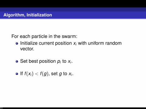
For each particle in the swarm:Initialize current position xi with uniform randomvector.
Set best position pi to xi .
If f (xi) < f (g), set g to xi .
Initialize velocity vi with uniform random vector.
9
Algorithm, Initialization
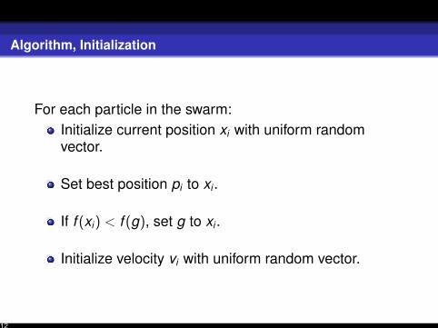
For each particle in the swarm:Initialize current position xi with uniform randomvector.
Set best position pi to xi .
If f (xi) < f (g), set g to xi .
Initialize velocity vi with uniform random vector.
10
Algorithm, Initialization
For each particle in the swarm:Initialize current position xi with uniform randomvector.
Set best position pi to xi .
If f (xi) < f (g), set g to xi .
Initialize velocity vi with uniform random vector.
11
Algorithm, Initialization
For each particle in the swarm:Initialize current position xi with uniform randomvector.
Set best position pi to xi .
If f (xi) < f (g), set g to xi .
Initialize velocity vi with uniform random vector.
12
Algorithm, Iteration
Until termination criterion, for each particle in the swarm,for each dimension, update position and velocity in the
following way:
(Note that I am leaving out indices for dimension, just tomake more readable.)
13

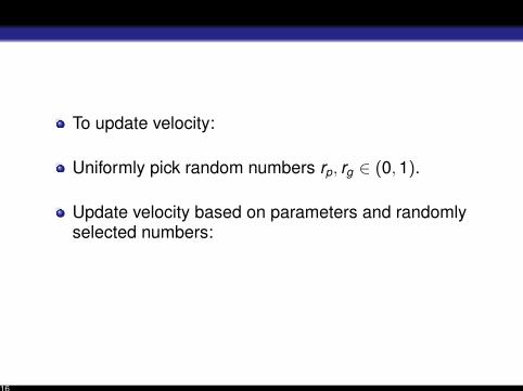
To update velocity:
Uniformly pick random numbers rp, rg ∈ (0,1).
Update velocity based on parameters and randomlyselected numbers:
vi = ωvi + φprp(pi − xi) + φgrg(g − xi).
14
To update velocity:
Uniformly pick random numbers rp, rg ∈ (0,1).
Update velocity based on parameters and randomlyselected numbers:
vi = ωvi + φprp(pi − xi) + φgrg(g − xi).
15
To update velocity:
Uniformly pick random numbers rp, rg ∈ (0,1).
Update velocity based on parameters and randomlyselected numbers:
vi = ωvi + φprp(pi − xi) + φgrg(g − xi).
16
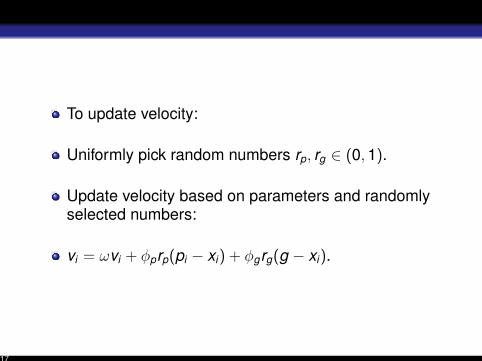
To update velocity:
Uniformly pick random numbers rp, rg ∈ (0,1).
Update velocity based on parameters and randomlyselected numbers:
vi = ωvi + φprp(pi − xi) + φgrg(g − xi).
17

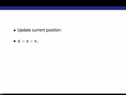
Update current position:
xi = xi + vi .
Check new f (xi) against particle and swarm, update ifimproved.
Keep going until termination.
18
Update current position:
xi = xi + vi .
Check new f (xi) against particle and swarm, update ifimproved.
Keep going until termination.
19
Update current position:
xi = xi + vi .
Check new f (xi) against particle and swarm, update ifimproved.
Keep going until termination.
20
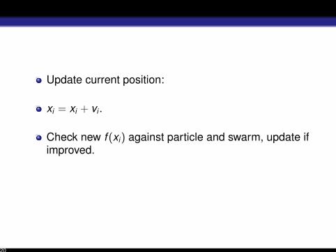
Update current position:
xi = xi + vi .
Check new f (xi) against particle and swarm, update ifimproved.
Keep going until termination.
21
Acceleration Coefficients
Recall:vi = ωvi + φprp(pi − xi) + φgrg(g − xi).
Cognitive component: models tendency of particles toreturn to previous best positions.
Social component: quantifies performance relative toneighbors.
22
Acceleration Coefficients
Recall:vi = ωvi + φprp(pi − xi) + φgrg(g − xi).
Cognitive component: models tendency of particles toreturn to previous best positions.
Social component: quantifies performance relative toneighbors.
23
Acceleration Coefficients
Recall:vi = ωvi + φprp(pi − xi) + φgrg(g − xi).
Cognitive component: models tendency of particles toreturn to previous best positions.
Social component: quantifies performance relative toneighbors.
24
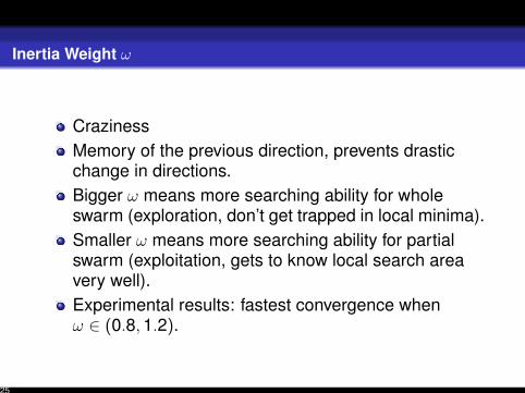
Inertia Weight ω
CrazinessMemory of the previous direction, prevents drasticchange in directions.Bigger ω means more searching ability for wholeswarm (exploration, don’t get trapped in local minima).Smaller ω means more searching ability for partialswarm (exploitation, gets to know local search areavery well).Experimental results: fastest convergence whenω ∈ (0.8,1.2).
25
Topology
Particles receive information from their neighbors.
Network of neighborhoods forms a graph.
Imitates different societies.
Characterize neighborhoods by connectivity,clustering.
26
Types of Topologies
Fully Connected Topology (gbest)Square Topology (Von Neumann)Ring Topology
27
Benefits
Makes few assumptions about the problem.
Doesn’t require differentiability (doesn’t use gradient).
Large spaces of candidate solutions.
Simple to implement.
28
Downsides
Does not guarantee optimality.
If maximum velocity too small, will only converge tolocal min.
Weak theoretical foundation.
Biased; solution more easily found if it is on axes.
29
Convergence
Based on experimental studies, relative to otherevolutionary algorithms, PSO has fast convergenceability but slow fine-tuning ability.Linearly decreasing inertia weight leads to betterperformance, but lacks global search ability.
30
Multiobjective/Constrained Optimization
Originally, PSO for single objective continuousproblem.Without constraints, sometimes particles want to gooutside search space.Particles initialized with only feasible solutions(speeds up search process).Only select feasible solutions as best values.Initialization takes longer.
31
Pareto Optimality
Search for multiple solutions.
Pick non-dominated solution.
Requires decision-maker at the end.
Aggregation: sum objective functions together usingweighted aggregation.
32
Pareto Optimality
Search for multiple solutions.
Pick non-dominated solution.
Requires decision-maker at the end.
Aggregation: sum objective functions together usingweighted aggregation.
33
Pareto Optimality
Search for multiple solutions.
Pick non-dominated solution.
Requires decision-maker at the end.
Aggregation: sum objective functions together usingweighted aggregation.
34
Pareto Optimality
Search for multiple solutions.
Pick non-dominated solution.
Requires decision-maker at the end.
Aggregation: sum objective functions together usingweighted aggregation.
35
Discrete Domains
Basic idea: map discrete search space to continuousspace, use a PSO, map result back to discrete space.Binary Particle Swarm Optimization – position isdiscrete, velocity is continuous.In velocity vector for agent i , vi , vij is probability thatxij = 1.
36
Applications
Human tremor analysis.
Biomedical Engineering.
Electric power and voltage management.
Machine scheduling.
Point Pattern Matching.
37
Applications
Human tremor analysis.
Biomedical Engineering.
Electric power and voltage management.
Machine scheduling.
Point Pattern Matching.
38
Applications
Human tremor analysis.
Biomedical Engineering.
Electric power and voltage management.
Machine scheduling.
Point Pattern Matching.
39
Applications
Human tremor analysis.
Biomedical Engineering.
Electric power and voltage management.
Machine scheduling.
Point Pattern Matching.
40
Applications
Human tremor analysis.
Biomedical Engineering.
Electric power and voltage management.
Machine scheduling.
Point Pattern Matching.
41
Open Shop Scheduling Problem
n jobs, m machines, each job has to be processed byeach machine at least once (m operations per job).Order irrevelant, processing time can be zero.Multi-objective: want to minimize completion time(makespan), minimize idle machine time.NP-hardTo use PSO, decode particle position into an activeschedule.
42
Permutation-Based PSO for Open Shop Scheduling Problem
Randomly generate group of particles represented bya permutation sequence (ordered list of operations)For n-job, m-machine problem, position of a particle isin m x n matrix.Let oij be operation of job j that must be processed onmachine i (these are the particle positions).Let the objective function be f(i,j), the earliest time atwhich oij can be finished.Minimize f , add the corresponding operations to theschedule.
43

Bibliography
44
Bibliography
Azlina, Nor, Mohamad Alias, Ammar Mohemmed, Kamarulzan Aziz."Particle Swarm Optimization for Constrained and MultiobjectiveProblems: A Brief Review." 2011 Conference on Management andArtificial Intelligence. PDER vol. 6 (2011).
Bai, Qinghai. "Analysis of Particle Swarm Optimization Algorithm."Computer and Information Science. Vol. 3, No. 1, February 2010.
45
Clerc, Maurice and James Kennedy. "The Particle Swarm - Explosion,Stability, and Convergence in a Multidimensional Complex Space." IEETranscations on Evolutionary Computation, Vol. 6, No 1, February 2002.
McCaffrey, James. "Particle Swarm Optimization." MSDN Magazine.August 2011.
Montes de Oca, Marco. "Particle Swarm Optimization." University ofDelaware, 2011.
P. N. Suganthan. "Particle Swarm Optimiser with NeighbourhoodOperator." Proceedings of the IEEE Congress on EvolutionaryComputation (CEC), pages 1958-1962, 1999.
http://tracer.uc3m.es/tws/pso/neighborhood.html
46