Embed Size (px)
Citation preview
Online: http://dust.ess.uci.edu/facts Updated: Mon 10th Jun, 2013, 11:45
Particle Size Distributions:Theory and Application to Aerosols, Clouds, and Soils
by Charlie ZenderUniversity of California, Irvine
Department of Earth System Science [email protected] of California Voice: (949) 891-2429Irvine, CA 92697-3100 Fax: (949) 824-3256
Copyright c© 1998–2013, Charles S. ZenderPermission is granted to copy, distribute and/or modify this document under the terms of the GNUFree Documentation License, Version 1.3 or any later version published by the Free SoftwareFoundation; with no Invariant Sections, no Front-Cover Texts, and no Back-Cover Texts. Thelicense is available online at http://www.gnu.org/copyleft/fdl.html.
Contents
Contents i
List of Tables 1
1 Introduction 11.1 Modal vs. Sectional Represenatation . . . . . . . . . . . . . . . . . . . . . . . . . 21.2 Nomenclature . . . . . . . . . . . . . . . . . . . . . . . . . . . . . . . . . . . . . 21.3 Distribution Function . . . . . . . . . . . . . . . . . . . . . . . . . . . . . . . . . 21.4 Probability Density Function . . . . . . . . . . . . . . . . . . . . . . . . . . . . . 3
1.4.1 Independent Variable . . . . . . . . . . . . . . . . . . . . . . . . . . . . . 3
2 Statistics of Size Distributions 42.1 Generic . . . . . . . . . . . . . . . . . . . . . . . . . . . . . . . . . . . . . . . . 42.2 Mean Size . . . . . . . . . . . . . . . . . . . . . . . . . . . . . . . . . . . . . . . 42.3 Variance . . . . . . . . . . . . . . . . . . . . . . . . . . . . . . . . . . . . . . . . 52.4 Standard Deviation . . . . . . . . . . . . . . . . . . . . . . . . . . . . . . . . . . 5
3 Cloud and Aerosol Size Distributions 53.1 Gamma Distribution . . . . . . . . . . . . . . . . . . . . . . . . . . . . . . . . . 53.2 Normal Distribution . . . . . . . . . . . . . . . . . . . . . . . . . . . . . . . . . . 53.3 Lognormal Distribution . . . . . . . . . . . . . . . . . . . . . . . . . . . . . . . . 6
3.3.1 Distribution Function . . . . . . . . . . . . . . . . . . . . . . . . . . . . . 63.3.2 Lognormal Relations . . . . . . . . . . . . . . . . . . . . . . . . . . . . . 83.3.3 Related Forms . . . . . . . . . . . . . . . . . . . . . . . . . . . . . . . . 14
3.3.4 Variance . . . . . . . . . . . . . . . . . . . . . . . . . . . . . . . . . . . . 163.3.5 Non-standard terminology . . . . . . . . . . . . . . . . . . . . . . . . . . 163.3.6 Bounded Distribution . . . . . . . . . . . . . . . . . . . . . . . . . . . . . 163.3.7 Statistics of Bounded Distributions . . . . . . . . . . . . . . . . . . . . . 173.3.8 Overlapping Distributions . . . . . . . . . . . . . . . . . . . . . . . . . . 183.3.9 Median Diameter . . . . . . . . . . . . . . . . . . . . . . . . . . . . . . . 193.3.10 Mode Diameter . . . . . . . . . . . . . . . . . . . . . . . . . . . . . . . . 193.3.11 Multimodal Distributions . . . . . . . . . . . . . . . . . . . . . . . . . . . 20
3.4 Higher Moments . . . . . . . . . . . . . . . . . . . . . . . . . . . . . . . . . . . 213.4.1 Aspherical Particles . . . . . . . . . . . . . . . . . . . . . . . . . . . . . 223.4.2 Normalization . . . . . . . . . . . . . . . . . . . . . . . . . . . . . . . . 23
4 Implementation in NCAR models 244.1 NCAR-Dust Model . . . . . . . . . . . . . . . . . . . . . . . . . . . . . . . . . . 244.2 Mie Scattering Model . . . . . . . . . . . . . . . . . . . . . . . . . . . . . . . . . 26
4.2.1 Input switches . . . . . . . . . . . . . . . . . . . . . . . . . . . . . . . . 264.2.2 Moments of Size Distribution . . . . . . . . . . . . . . . . . . . . . . . . 264.2.3 Generating Properties for Multi-Bin Distributions . . . . . . . . . . . . . . 27
5 Appendix 275.1 Properties of Gaussians . . . . . . . . . . . . . . . . . . . . . . . . . . . . . . . . 275.2 Error Function . . . . . . . . . . . . . . . . . . . . . . . . . . . . . . . . . . . . . 275.3 Command Line Switches for mie Code . . . . . . . . . . . . . . . . . . . . . . . 28
Bibliography 58
Index 61
List of Tables
1 Lognormal Distribution Relations . . . . . . . . . . . . . . . . . . . . . . . . . . 92 Measured Lognormal Dust Size Distributions . . . . . . . . . . . . . . . . . . . . 113 Analytic Lognormal Statistics . . . . . . . . . . . . . . . . . . . . . . . . . . . . 134 Source Size Distribution . . . . . . . . . . . . . . . . . . . . . . . . . . . . . . . 255 Command Line Switches . . . . . . . . . . . . . . . . . . . . . . . . . . . . . . . 296 SWNB Output Fields . . . . . . . . . . . . . . . . . . . . . . . . . . . . . . . . . 377 CLM Output Fields . . . . . . . . . . . . . . . . . . . . . . . . . . . . . . . . . . 45
1 Introduction
This document describes mathematical and computational considerations pertaining to size distri-butions. The application of statistical theory to define meaningful and measurable parameters for
2 1 INTRODUCTION
defining generic size distributions is presented in §2. The remaining sections apply these defini-tions to the size distributions most commonly used to describe clouds and aerosol size distributionsin the meteorological literature. Currently, only the lognormal distribution is presented.
1.1 Modal vs. Sectional Represenatationmdlsxn Lu and Bowman (2004) designed and optimal non-linear least squares-based procedure forconverting from sectional to modal representations.
1.2 Nomenclaturenomenclature There is a bewildering variety of nomenclature associated with size distributions,probability density functions, and statistics thereof. The nomenclature in this article generally fol-lows the standard references, (see, e.g., Hansen and Travis, 1974; Patterson and Gillette, 1977;Press et al., 1988; Flatau et al., 1989; Seinfeld and Pandis, 1997), at least where those referencesare in agreement. Quantities whose nomenclature is often confusing, unclear, or simply not stan-dardized are discussed in the text.
1.3 Distribution FunctionThis section follows the carefully presented discussion of Flatau et al. (1989). The size distributionfunction nn(r) is defined such that nn(r) dr is the total concentration (number per unit volume ofair, or # m−3) of particles with sizes in the domain [r, r + dr]. The total number concentration ofparticles N0 is obtained by integrating nn(r) over all sizes
N0 =
∫ ∞0
nn(r) dr (1)
The size distribution function is also called the spectral density function. The dimensions of nn(r)and N0 are # m−3 m−1 and # m−3, respectively. Note that nn(r) is only normalized if N0 = 1.0 (cf.Section 3.4.2).
Often N0 is not an observable quantity. A variety of functional forms, some of which are over-loaded for clarity, describe the number concentrations actually measured by instruments. Typicallyan instrument has a lower detection limit rmin and an upper detection limit rmax of particle sizeswhich it can measure.
N(r < rmax) =
∫ rmax
0
nn(r) dr (2)
N(r > rmax) =
∫ ∞rmax
nn(r) dr (3)
N(rmin, rmax) = N(rmin < r < rmax) =
∫ rmax
rmin
nn(r) dr (4)
Equations (2)–(4) define the cumulative concentration, lower bound concentration, and truncatedconcentration, respectively. The cumulative concentration is used to define the median radius rn.
1.4 Probability Density Function 3
Half the particles are larger and half smaller than rn
N(r < rn) = N(r > rn) =N0
2(5)
These functions are often used to define nn(r) via
nn(r) =dN
dr(6)
Note that the concentration nomenclature in (6) is N not N(r). Using N(r) would indicate thatthe concentration has not been completely integrated over all sizes. By definition, the total concen-tration N0 is integrated over all sizes, as defined by (1). A concentration denoted N(r) makes nosense without an associated size bin width ∆r, or truncation convention, as in (2)–(4). We try touse N and N0 for normalized (N = 1) and non-normalized (N0 6= 1, i.e., absolute concentrations).However this convention is not absolute and (1) defines both N and N0.
1.4 Probability Density FunctionDescribing size distributions is easier when they are normalized into probability density functions,or PDFs. In this context, a PDF is a size distribution function normalized to unity over the domainof interest, i.e., p(r) = Cnnn(r) where the normalization constant Cn is defined such that∫ ∞
0
p(r) dr = 1 (7)
In the following sections we usually work with PDFs because this normalization property is veryconvenient mathematically. Comparing (7) and (1), it is clear that the normalization constant Cnwhich transforms a size distribution function (1) into a PDF p(r) is N−1
0
p(r) =1
N0
nn(r) (8)
1.4.1 Choice of Independent Variable
The merits of using radius r, diameter D, or some other dimension L, as the independent variableof a size distribution depend on the application. In radiative transfer applications, r prevails in theliterature probably because it is favored in electromagnetic and Mie theory. There is, however,a growing recognition of the importance of aspherical particles in planetary atmospheres. Defin-ing an equivalent radius or equivalent diameter for these complex shapes is not straighforward(consider, e.g., a bullet rosette ice crystal). Important differences exist among the competing defi-nitions, such as equivalent area spherical radius, equivalent volume spherical radius, (e.g., Ebertand Curry, 1992; McFarquhar and Heymsfield, 1997).
A direct property of aspherical particles which can often be measured is its maximum dimen-sion, i.e., the greatest distance between any two surface points of the particle. This maximumdimension, usually called L, has proven to be useful for characterizing size distributions of as-pherical particles. For a sphere, L is also the diameter. Analyses of mineral dust sediments in icecore deposits or sediment traps, for example, are usually presented in terms of L. The surface area
4 2 STATISTICS OF SIZE DISTRIBUTIONS
and volume of ice crystals have been computed in terms of power laws of L (e.g., Heymsfield andPlatt, 1984; Takano and Liou, 1995). Since models usually lack information regarding the shape ofparticles (early exceptions include Zender and Kiehl, 1994; Chen and Lamb, 1994), most modelersassume spherical particles, especially for aerosols. Thus, the advantages of using the diameter Das the independent variable in size distribution studies include: D is the dimension often reportedin measurements; D is more analogous than r to L.
The remainder of this manuscript assumes spherical particles where r and D are equally usefulindependent variables. Unless explicitly noted, our convention will be to use D as the independentvariable. Thus, it is useful to understand the rules governing conversion of PDFs from D to r andthe reverse.
Consider two distinct analytic representations of the same underlying size distribution. Thefirst, nDn (D), expresses the differential number concentration per unit diameter. The second, nrn(r),expresses the differential number concentration per unit radius. Both nDn (D) and nrn(r) share thesame dimensions, # m−3 m−1.
D = 2r (9)dD = 2 dr (10)
nDn (D) dD = nrn(r) dr (11)
nDn (D) =1
2nrn(r) (12)
2 Statistics of Size Distributions
2.1 GenericConsider an arbitrary function g(x) which applies over the domain of the size distribution p(x).For now the exact definition of g is irrelevant, but imagine that g(x) describes the variation of somephysically meaningful quantity (e.g., area) with size. The mean value of g is the integral of g overthe domain of the size distribution, weighted at each point by the concentration of particles
g =
∫ ∞0
g(x) p(x) dx (13)
Once p(x) is known, it is always possible to compute g for any desired quantity g. Typical quan-tities represented by g(x) are size, g(x) = x; area, g(x) = A(x) ∝ x2; and volume g(x) =V (x) ∝ x3. More complicated statistics represented by g(x) include variance, g(x) = (x − x)2.The remainder of this section considers some of these examples in more detail.
2.2 Mean SizeThe number mean size x of a size distribution p(x) is defined as
x =
∫ ∞0
p(x)x dx (14)
Synonyms for number mean size include mean size, average size, arithmetic mean size, andnumber-weighted mean size (Hansen and Travis, 1974). Flatau et al. (1989) define Dn ≡ D,a convention we adopt in the following.
2.3 Variance 5
2.3 VarianceThe variance σ2
x of a size distribution p(x) is defined in accord with the statistical variance of acontinuous mathematical distribution.
σ2x =
∫ ∞0
p(x)(x− x)2 dx (15)
The variance measures the mean squared-deviation of the distribution from its mean value. Theunits of σ2
x are [m2]. Because σ2x is a complicated function for standard aerosol and cloud size
distributions, many prefer to work with an alternate definition of variance, called the effectivevariance.
The effective variance σ2x,eff of a size distribution p(x) is the variance about the effective size
of the distribution, normalized by xeff (e.g., Hansen and Travis, 1974)
σ2x,eff =
1
x2eff
∫ ∞0
p(x)(x− xeff)2 x2 dx (16)
Because of the x−2eff normalization, σ2
x,eff is non-dimensional in contrast to typical variances, e.g.,(15). In the terminology of Hansen and Travis (1974), σ2
x,eff = v.
2.4 Standard DeviationThe standard deviation σx of a size distribution p(x) is the square root of the variance (15),
σx =√σ2x (17)
σx has units of [m]. For standard aerosol and cloud size distributions, σx is an ugly expression.Therefore many authors prefer to work with alternate definitions of standard deviation. Unfortu-nately, nomenclature for these alternate definitions is not standardized.
3 Cloud and Aerosol Size Distributions3.1 Gamma Distribution
Statistics of the gamma distribution are presented in http://asd-www.larc.nasa.gov/
˜yhu/paper/thesisall/node8.html. Currently, the aerosol property program mie im-plements gamma distributions in a limited sense.
3.2 Normal Distribution
The normal distribution is the most common statistical distribution. The normal distribution n(x)is expressed in terms of its mean x (14) and standard deviation σx (17)
n(x) =1√
2πσxexp
[−1
2
(x− xσx
)2]
(18)
6 3 CLOUD AND AEROSOL SIZE DISTRIBUTIONS
With our standard nomenclature for number distribution nn and particles diameter D, (18) appearsas
nn(D) ≡ dN
dD=
1√2πσD
exp
[−1
2
(D − Dn
σD
)2]
(19)
The cumulative normal distribution is called the error function and is discussed in Section (5.1).Integration of the error function shows that 68.3% of the values of (19) are in Dn ± σD, 95.4% arein Dn ± 2σD, and 99.7% are in Dn ± 3σD.
3.3 Lognormal Distribution
The lognormal distribution is perhaps the most commonly used analytic expression in aerosolstudies.
3.3.1 Distribution Function
In a lognormal distribution, the logarithm of abscissa is normally distributed (Section 3.2). Substi-tuting x = lnD into (18) yields
nn(lnD) ≡ dN
d lnD=
1√2π lnσg
exp
−1
2
(lnD − ln Dn
lnσg
)2 (20)
where σg and Dn are parameters whose physical significance is to be defined. In particular, there isno closed-form algebraic relationship between σD (19) and σg (20). The former is a true standarddeviation and the properties of the latter are as yet unknown.
Substituting d lnD = D−1 dD in (20) leads to the most commonly used form the lognormaldistribution function
nn(D) ≡ dN
dD=
1√2πD lnσg
exp
−1
2
(ln(D/Dn)
lnσg
)2 (21)
One of the most confusing aspects of size distributions in the meteorological literature is in theusage of σg, the geometric standard deviation. Some researchers (e.g., Flatau et al., 1989) prefera different formulation (21) which is equivalent to
nn(D) =1√
2π σgDexp
−1
2
(ln(D/Dn)
σg
)2 (22)
whereσg ≡ lnσg (23)
In practice, (21) is used more widely than (22) and we adopt (21) in the following.
3.3 Lognormal Distribution 7
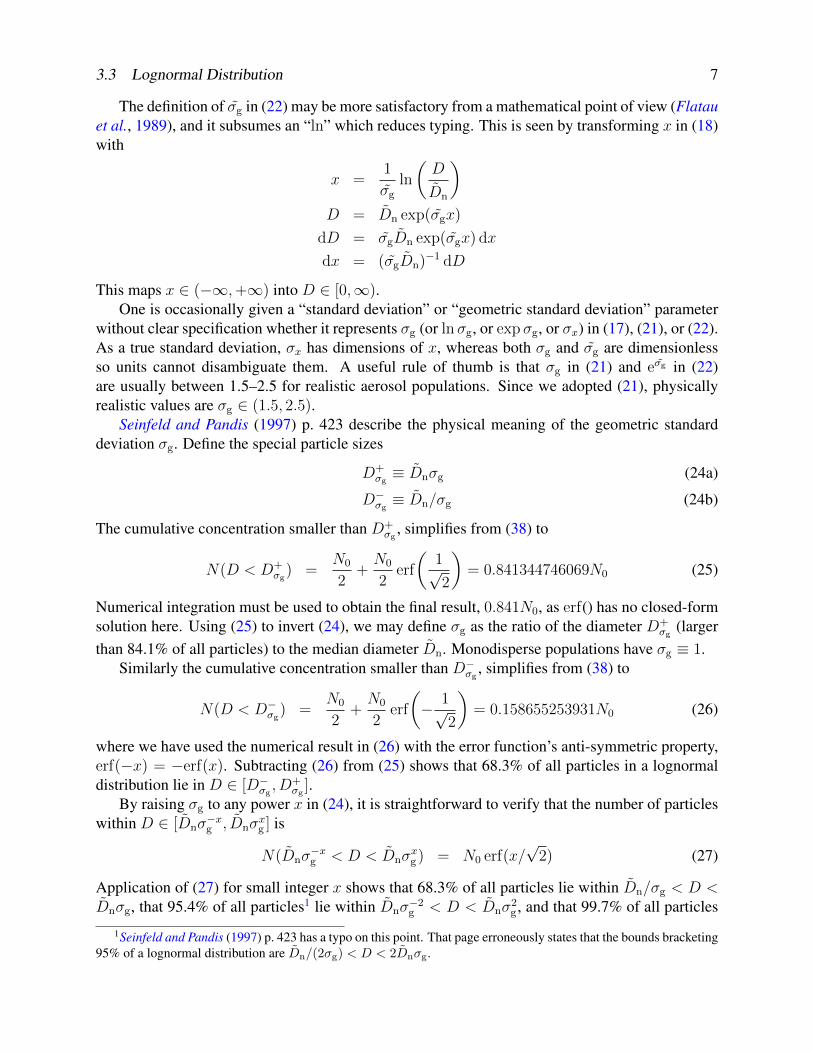
The definition of σg in (22) may be more satisfactory from a mathematical point of view (Flatauet al., 1989), and it subsumes an “ln” which reduces typing. This is seen by transforming x in (18)with
x =1
σg
ln
(D
Dn
)D = Dn exp(σgx)
dD = σgDn exp(σgx) dx
dx = (σgDn)−1 dD
This maps x ∈ (−∞,+∞) into D ∈ [0,∞).One is occasionally given a “standard deviation” or “geometric standard deviation” parameter
without clear specification whether it represents σg (or lnσg, or expσg, or σx) in (17), (21), or (22).As a true standard deviation, σx has dimensions of x, whereas both σg and σg are dimensionlessso units cannot disambiguate them. A useful rule of thumb is that σg in (21) and eσg in (22)are usually between 1.5–2.5 for realistic aerosol populations. Since we adopted (21), physicallyrealistic values are σg ∈ (1.5, 2.5).
Seinfeld and Pandis (1997) p. 423 describe the physical meaning of the geometric standarddeviation σg. Define the special particle sizes
D+σg≡ Dnσg (24a)
D−σg≡ Dn/σg (24b)
The cumulative concentration smaller than D+σg
, simplifies from (38) to
N(D < D+σg
) =N0
2+N0
2erf
(1√2
)= 0.841344746069N0 (25)
Numerical integration must be used to obtain the final result, 0.841N0, as erf() has no closed-formsolution here. Using (25) to invert (24), we may define σg as the ratio of the diameter D+
σg(larger
than 84.1% of all particles) to the median diameter Dn. Monodisperse populations have σg ≡ 1.Similarly the cumulative concentration smaller than D−σg
, simplifies from (38) to
N(D < D−σg) =
N0
2+N0
2erf
(− 1√
2
)= 0.158655253931N0 (26)
where we have used the numerical result in (26) with the error function’s anti-symmetric property,erf(−x) = −erf(x). Subtracting (26) from (25) shows that 68.3% of all particles in a lognormaldistribution lie in D ∈ [D−σg
, D+σg
].By raising σg to any power x in (24), it is straightforward to verify that the number of particles
within D ∈ [Dnσ−xg , Dnσ
xg ] is
N(Dnσ−xg < D < Dnσ
xg ) = N0 erf(x/
√2) (27)
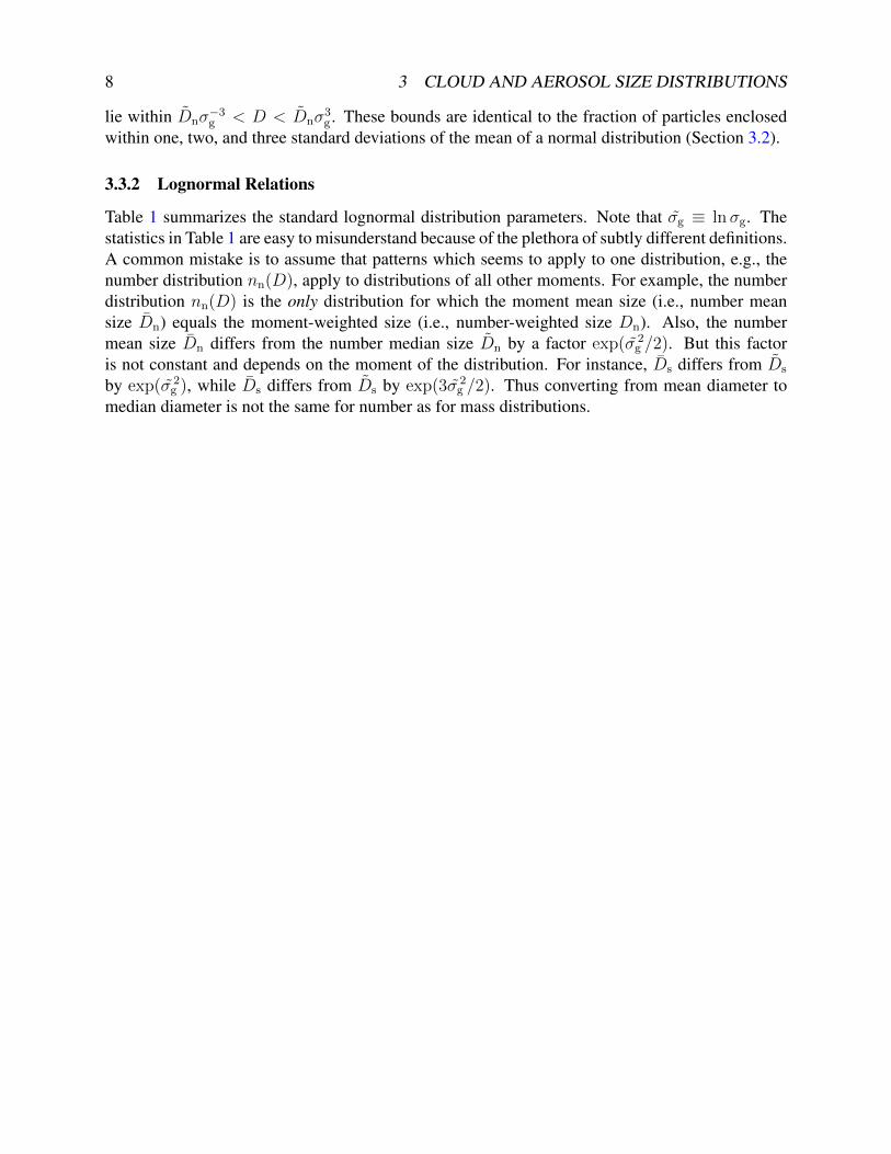
Application of (27) for small integer x shows that 68.3% of all particles lie within Dn/σg < D <Dnσg, that 95.4% of all particles1 lie within Dnσ
−2g < D < Dnσ
2g , and that 99.7% of all particles
1Seinfeld and Pandis (1997) p. 423 has a typo on this point. That page erroneously states that the bounds bracketing95% of a lognormal distribution are Dn/(2σg) < D < 2Dnσg.
8 3 CLOUD AND AEROSOL SIZE DISTRIBUTIONS
lie within Dnσ−3g < D < Dnσ
3g . These bounds are identical to the fraction of particles enclosed
within one, two, and three standard deviations of the mean of a normal distribution (Section 3.2).
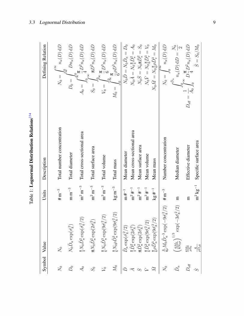
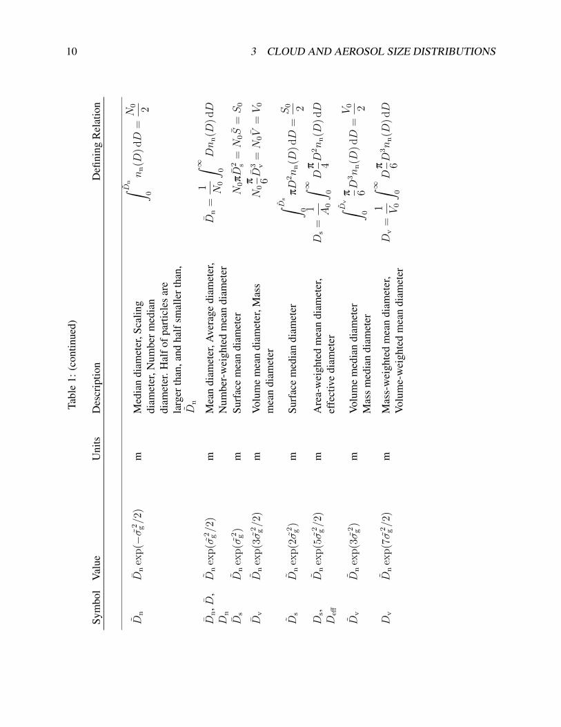
3.3.2 Lognormal Relations
Table 1 summarizes the standard lognormal distribution parameters. Note that σg ≡ lnσg. Thestatistics in Table 1 are easy to misunderstand because of the plethora of subtly different definitions.A common mistake is to assume that patterns which seems to apply to one distribution, e.g., thenumber distribution nn(D), apply to distributions of all other moments. For example, the numberdistribution nn(D) is the only distribution for which the moment mean size (i.e., number meansize Dn) equals the moment-weighted size (i.e., number-weighted size Dn). Also, the numbermean size Dn differs from the number median size Dn by a factor exp(σg
2/2). But this factoris not constant and depends on the moment of the distribution. For instance, Ds differs from Ds
by exp(σg2), while Ds differs from Ds by exp(3σg
2/2). Thus converting from mean diameter tomedian diameter is not the same for number as for mass distributions.
3.3 Lognormal Distribution 9
Tabl
e1:
Log
norm
alD
istr
ibut
ion
Rel
atio
ns23
4
Sym
bol
Val
ueU
nits
Des
crip
tion
Defi
ning
Rel
atio
n
N0
N0
#m−
3To
taln
umbe
rcon
cent
ratio
nN
0=
∫ ∞ 0
nn(D
)dD
D0
N0D
nex
p(σ
g2)
mm−
3To
tald
iam
eter
D0
=
∫ ∞ 0
Dn
n(D
)dD
A0
π 4N
0D
2 nex
p(σ
g2/2
)m
2m−
3To
talc
ross
-sec
tiona
lare
aA
0=
∫ ∞ 0
π 4D
2n
n(D
)dD
S0
πN
0D
2 nex
p(2σ
g2)
m2
m−
3To
tals
urfa
cear
eaS
0=
∫ ∞ 0
πD
2n
n(D
)dD
V0
π 6N
0D
3 nex
p(9σ
g2/2
)m
3m−
3To
talv
olum
eV
0=
∫ ∞ 0
π 6D
3n
n(D
)dD
M0
π 6N
0ρD
3 nex
p(9σ
g2/2
)kg
m−
3To
talm
ass
M0
=
∫ ∞ 0
π 6ρD
3n
n(D
)dD
DD
nex
p(σ
g2/2
)m
#−1
Mea
ndi
amet
erN
0D
=N
0D
n=D
0
Aπ 4D
2 nex
p(2σ
g2)
m2
#−1
Mea
ncr
oss-
sect
iona
lare
aN
0A
=N
0π 4D
2 s=A
0
SπD
2 nex
p(2σ
g2)
m2
#−1
Mea
nsu
rfac
ear
eaN
0S
=N
0πD
2 s=S
0
Vπ 6D
3 nex
p(9σ
g2/2
)m
3#−
1M
ean
volu
me
N0V
=N
0π 6D
3 v=V
0
Mπ 6ρD
3 nex
p(9σ
g2/2
)kg
#−1
Mea
nm
ass
N0M
=N
0π 6ρD
3 v=M
0
N0
6 πρM
0D−
3n
exp(−
9σg2/2
)#
m−
3N
umbe
rcon
cent
ratio
nN
0=
∫ ∞ 0
nn(D
)dD
Dn
( 6M
0
πN
0ρ
) 1/3ex
p(−
3σg2/2
)m
Med
ian
diam
eter
∫ D n 0
nn(D
)dD
=N
0 2
Deff
6M
0
ρS
0m
Eff
ectiv
edi
amet
erD
eff=
1 A0
∫ ∞ 0
Dπ 4D
2n
n(D
)dD
S6
ρD
eff
m2
kg−
1Sp
ecifi
csu
rfac
ear
eaS
=S
0/M
0
10 3 CLOUD AND AEROSOL SIZE DISTRIBUTIONS
Tabl
e1:
(con
tinue
d)
Sym
bol
Val
ueU
nits
Des
crip
tion
Defi
ning
Rel
atio
n
Dn
Dn
exp(−σ
g2/2
)m
Med
ian
diam
eter
,Sca
ling
diam
eter
,Num
berm
edia
ndi
amet
er.H
alfo
fpar
ticle
sar
ela
rger
than
,and
half
smal
lert
han,
Dn
∫ D n 0
nn(D
)dD
=N
0 2
Dn,D
,D
n
Dn
exp(σ
g2/2
)m
Mea
ndi
amet
er,A
vera
gedi
amet
er,
Num
ber-
wei
ghte
dm
ean
diam
eter
Dn
=1 N
0
∫ ∞ 0
Dn
n(D
)dD
Ds
Dn
exp(σ
g2)
mSu
rfac
em
ean
diam
eter
N0πD
2 s=N
0S
=S
0
Dv
Dn
exp(3σ
g2/2
)m
Volu
me
mea
ndi
amet
er,M
ass
mea
ndi
amet
erN
0π 6D
3 v=N
0V
=V
0
Ds
Dn
exp(2σ
g2)
mSu
rfac
em
edia
ndi
amet
er∫ D s 0
πD
2n
n(D
)dD
=S
0 2
Ds,
Deff
Dn
exp(5σ
g2/2
)m
Are
a-w
eigh
ted
mea
ndi
amet
er,
effe
ctiv
edi
amet
erD
s=
1 A0
∫ ∞ 0
Dπ 4D
2n
n(D
)dD
Dv
Dn
exp(3σ
g2)
mVo
lum
em
edia
ndi
amet
erM
ass
med
ian
diam
eter
∫ D v 0
π 6D
3n
n(D
)dD
=V
0 2
Dv
Dn
exp(7σ
g2/2
)m
Mas
s-w
eigh
ted
mea
ndi
amet
er,
Volu
me-
wei
ghte
dm
ean
diam
eter
Dv
=1 V0
∫ ∞ 0
Dπ 6D
3n
n(D
)dD
3.3 Lognormal Distribution 11
For brevity Table 1 presents the lognormal relations in terms of diamterD. Change the relationsto befunctions of radius r is straightforward. For example, direct substitution of D = 2r into (21)yields
nn(D) =1√
2π 2r lnσg
exp
[−1
2
(ln(2r/2rn)
lnσg
)2]
=1
2
1√2π r lnσg
exp
[−1
2
(ln(r/rn)
lnσg
)2]
=1
2nrn(r) (28)
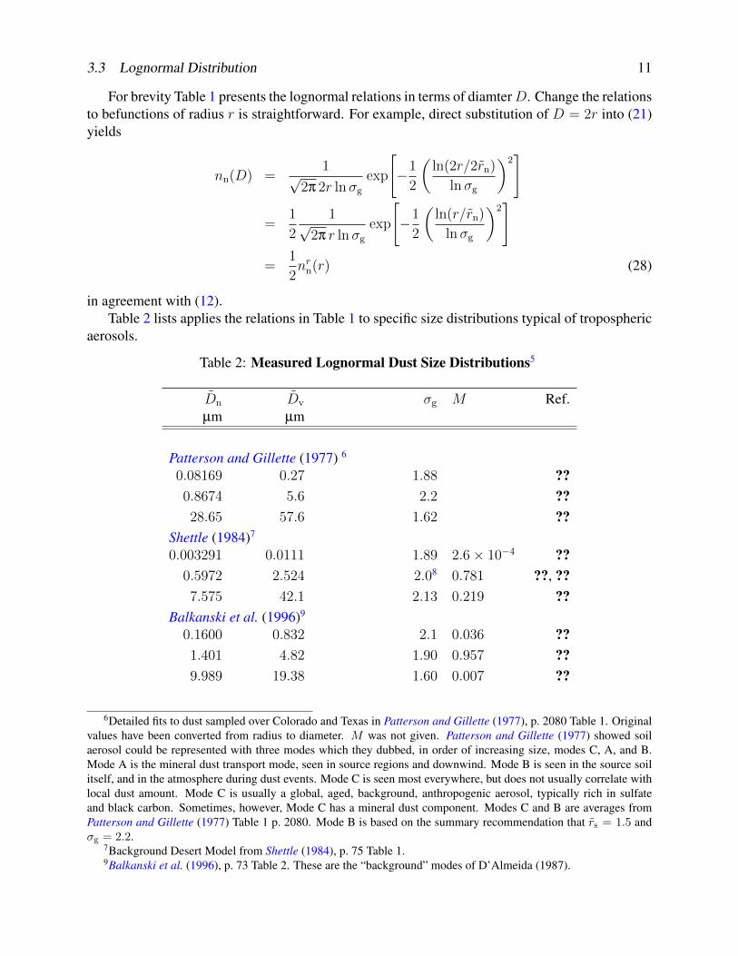
in agreement with (12).Table 2 lists applies the relations in Table 1 to specific size distributions typical of tropospheric
aerosols.
Table 2: Measured Lognormal Dust Size Distributions5
Dn Dv σg M Ref.µm µm
Patterson and Gillette (1977) 6
0.08169 0.27 1.88 ??0.8674 5.6 2.2 ??28.65 57.6 1.62 ??
Shettle (1984)7
0.003291 0.0111 1.89 2.6× 10⁻⁴ ??0.5972 2.524 2.08 0.781 ??, ??7.575 42.1 2.13 0.219 ??
Balkanski et al. (1996)9
0.1600 0.832 2.1 0.036 ??1.401 4.82 1.90 0.957 ??9.989 19.38 1.60 0.007 ??
6Detailed fits to dust sampled over Colorado and Texas in Patterson and Gillette (1977), p. 2080 Table 1. Originalvalues have been converted from radius to diameter. M was not given. Patterson and Gillette (1977) showed soilaerosol could be represented with three modes which they dubbed, in order of increasing size, modes C, A, and B.Mode A is the mineral dust transport mode, seen in source regions and downwind. Mode B is seen in the source soilitself, and in the atmosphere during dust events. Mode C is seen most everywhere, but does not usually correlate withlocal dust amount. Mode C is usually a global, aged, background, anthropogenic aerosol, typically rich in sulfateand black carbon. Sometimes, however, Mode C has a mineral dust component. Modes C and B are averages fromPatterson and Gillette (1977) Table 1 p. 2080. Mode B is based on the summary recommendation that rs = 1.5 andσg = 2.2.
7Background Desert Model from Shettle (1984), p. 75 Table 1.9Balkanski et al. (1996), p. 73 Table 2. These are the “background” modes of D’Almeida (1987).
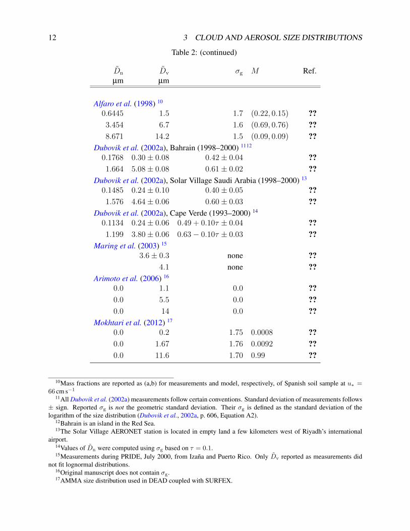
12 3 CLOUD AND AEROSOL SIZE DISTRIBUTIONS
Table 2: (continued)
Dn Dv σg M Ref.µm µm
Alfaro et al. (1998) 10
0.6445 1.5 1.7 (0.22, 0.15) ??3.454 6.7 1.6 (0.69, 0.76) ??8.671 14.2 1.5 (0.09, 0.09) ??
Dubovik et al. (2002a), Bahrain (1998–2000) 1112
0.1768 0.30± 0.08 0.42± 0.04 ??1.664 5.08± 0.08 0.61± 0.02 ??
Dubovik et al. (2002a), Solar Village Saudi Arabia (1998–2000) 13
0.1485 0.24± 0.10 0.40± 0.05 ??1.576 4.64± 0.06 0.60± 0.03 ??
Dubovik et al. (2002a), Cape Verde (1993–2000) 14
0.1134 0.24± 0.06 0.49 + 0.10τ ± 0.04 ??1.199 3.80± 0.06 0.63− 0.10τ ± 0.03 ??
Maring et al. (2003) 15
3.6± 0.3 none ??4.1 none ??
Arimoto et al. (2006) 16
0.0 1.1 0.0 ??0.0 5.5 0.0 ??0.0 14 0.0 ??
Mokhtari et al. (2012) 17
0.0 0.2 1.75 0.0008 ??0.0 1.67 1.76 0.0092 ??0.0 11.6 1.70 0.99 ??
10Mass fractions are reported as (a,b) for measurements and model, respectively, of Spanish soil sample at u∗ =66 cm s−1
11All Dubovik et al. (2002a) measurements follow certain conventions. Standard deviation of measurements follows± sign. Reported σg is not the geometric standard deviation. Their σg is defined as the standard deviation of thelogarithm of the size distribution (Dubovik et al., 2002a, p. 606, Equation A2).
12Bahrain is an island in the Red Sea.13The Solar Village AERONET station is located in empty land a few kilometers west of Riyadh’s international
airport.14Values of Dn were computed using σg based on τ = 0.1.15Measurements during PRIDE, July 2000, from Izana and Puerto Rico. Only Dv reported as measurements did
not fit lognormal distributions.16Original manuscript does not contain σg.17AMMA size distribution used in DEAD coupled with SURFEX.
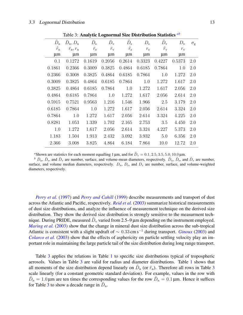
3.3 Lognormal Distribution 13
Table 3: Analytic Lognormal Size Distribution Statistics ab
Dn Dn, Dn Ds Dv Ds Ds Dv Dv σg
rn rn, rn rs rv rs rs rv rv
µm µm µm µm µm µm µm µm0.1 0.1272 0.1619 0.2056 0.2614 0.3323 0.4227 0.5373 2.0
0.1861 0.2366 0.3009 0.3825 0.4864 0.6185 0.7864 1.0 2.0
0.2366 0.3008 0.3825 0.4864 0.6185 0.7864 1.0 1.272 2.0
0.3009 0.3825 0.4864 0.6185 0.7864 1.0 1.272 1.617 2.0
0.3825 0.4864 0.6185 0.7864 1.0 1.272 1.617 2.056 2.0
0.4864 0.6185 0.7864 1.0 1.272 1.617 2.056 2.614 2.0
0.5915 0.7521 0.9563 1.216 1.546 1.966 2.5 3.179 2.0
0.6185 0.7864 1.0 1.272 1.617 2.056 2.614 3.324 2.0
0.7864 1.0 1.272 1.617 2.056 2.614 3.324 4.225 2.0
0.8281 1.053 1.339 1.702 2.165 2.753 3.5 4.450 2.0
1.0 1.272 1.617 2.056 2.614 3.324 4.227 5.373 2.0
1.183 1.504 1.913 2.432 3.092 3.932 5.0 6.356 2.0
2.366 3.008 3.825 4.864 6.184 7.864 10.0 12.72 2.0
aShown are statistics for each moment equalling 1 µm, and for Dv = 0.1, 2.5, 3.5, 5.0, 10.0 µm.b Dn, Ds, and Dv are number, surface, and volume-mean diameters, respectively. Dn, Ds, and Dv are number,
surface, and volume median diameters, respectively. Dn, Ds, and Dv are number, surface, and volume-weighteddiameters, respectively.
Perry et al. (1997) and Perry and Cahill (1999) describe measurements and transport of dustacross the Atlantic and Pacific, respectively. Reid et al. (2003) summarize historical measurementsof dust size distributions, and analyze the influence of measurement technique on the derived sizedistribution. They show the derived size distribution is strongly sensitive to the measurment tech-nique. During PRIDE, measured Dv varied from 2.5–9 µm depending on the instrument employed.Maring et al. (2003) show that the change in mineral dust size distribution across the sub-tropicalAtlantic is consistent with a slight updraft of ∼ 0.33 cm s−1 during transport. Ginoux (2003) andColarco et al. (2003) show that the effects of asphericity on particle settling velocity play an im-portant role in maintaining the large particle tail of the size distribution during long range transport.
Table 3 applies the relations in Table 1 to specific size distributions typical of troposphericaerosols. Values in Table 3 are valid for radius and diameter distributions. Table 1 shows thatall moments of the size distribution depend linearly on Dn (or rn). Therefore all rows in Table 3scale linearly (for a constant geometric standard deviation). For example, values in the row withDn = 1.0 µm are ten times the corresponding values for the row Dn = 0.1 µm. Hence it sufficesfor Table 3 to show a decade range in Dn.
14 3 CLOUD AND AEROSOL SIZE DISTRIBUTIONS
3.3.3 Related Forms
Many important applications make available size distribution information in a form similar to, buthard to recognize as, the analytic lognormal PDF (21). The Aerosol Robotic Network, AERONET ,for example, retrieves size distributions from solar almucantar radiances18 (Dubovik and King,2000; Dubovik et al., 2000, 2002b). AERONET labels the retrieved size distribution dV (r)/d ln rand reports the values in [µm3 µm−2] units. The correspondence between the AERONET retrievalsand dN/d ln r (21) in [# m−3 m−1] units is not exactly clear. Unfortunately, Table 1 does not helpmuch here. Let us now show how to bridge the gap between theory and measurement.
First, total distributions contain N0 particles per unit volume and thus N0 applies as a multi-plicative factor to (21)
nn(D) =N0√
2πD lnσg
exp
−1
2
(ln(D/Dn)
lnσg
)2 (29)
Note that (29) is only normalized if N0 = 1.0 (cf. Section 3.4.2).Applying (6) to (29) yields
dN
dD=
N0√2πD lnσg
exp
−1
2
(ln(D/Dn)
lnσg
)2 (30)
Multiplying each side of (30) by D and substituting d lnD = D−1 dD leads to
dN
d lnD=
N0√2π lnσg
exp
−1
2
(ln(D/Dn)
lnσg
)2 (31)
The derivative in (31) is with respect to the logarithm of the diameter. The change in the inde-pendent variable of differentiation defines a new distribution which could be written nn(lnD) todistinguish it from the normal linear distribution nn(D) (6). However, the nomenclature nn(lnD)could be misinterpreted. We follow Seinfeld and Pandis (1997) and denote logarithmically-defineddistributions with a superscript e on the distribution that re-inforces the use of lnD as the indepen-dent variable
nen(lnD) ≡ nn(lnD) ≡ dN
d lnD(32)
The SI units of nn(D) (6) and nen(lnD) (32) are [# m−3 m−1] and [# m−3], respectively.
Remote sensing applications often retrieve columnar distributions rather than volumetric dis-tributions. The columnar number distribution nc
n(D), for example, is simply the vertical integral
18 The almucantar radiances are radiance measurements in a circle of equal scattering angle centered in a planeabout the Sun, i.e., radiance measurements at known forward scattering phase function angles.
3.3 Lognormal Distribution 15
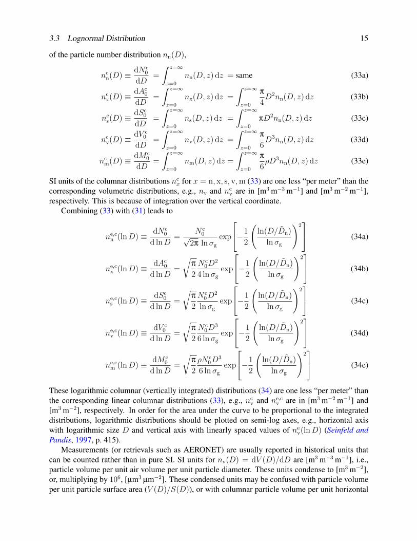
of the particle number distribution nn(D),
ncn(D) ≡ dN c
0
dD=
∫ z=∞
z=0
nn(D, z) dz = same (33a)
ncx(D) ≡ dAc
0
dD=
∫ z=∞
z=0
nx(D, z) dz =
∫ z=∞
z=0
π
4D2nn(D, z) dz (33b)
ncs(D) ≡ dSc
0
dD=
∫ z=∞
z=0
ns(D, z) dz =
∫ z=∞
z=0
πD2nn(D, z) dz (33c)
ncv(D) ≡ dV c
0
dD=
∫ z=∞
z=0
nv(D, z) dz =
∫ z=∞
z=0
π
6D3nn(D, z) dz (33d)
ncm(D) ≡ dM c
0
dD=
∫ z=∞
z=0
nm(D, z) dz =
∫ z=∞
z=0
π
6ρD3nn(D, z) dz (33e)
SI units of the columnar distributions ncx for x = n, x, s, v,m (33) are one less “per meter” than the
corresponding volumetric distributions, e.g., nv and ncv are in [m3 m−3 m−1] and [m3 m−2 m−1],
respectively. This is because of integration over the vertical coordinate.Combining (33) with (31) leads to
ne,cn (lnD) ≡ dN c
0
d lnD=
N c0√
2π lnσg
exp
−1
2
(ln(D/Dn)
lnσg
)2 (34a)
ne,cx (lnD) ≡ dAc
0
d lnD=
√π
2
N c0D
2
4 lnσg
exp
−1
2
(ln(D/Dn)
lnσg
)2 (34b)
ne,cs (lnD) ≡ dSc
0
d lnD=
√π
2
N c0D
2
lnσg
exp
−1
2
(ln(D/Dn)
lnσg
)2 (34c)
ne,cv (lnD) ≡ dV c
0
d lnD=
√π
2
N c0D
3
6 lnσg
exp
−1
2
(ln(D/Dn)
lnσg
)2 (34d)
ne,cm (lnD) ≡ dM c
0
d lnD=
√π
2
ρN c0D
3
6 lnσg
exp
−1
2
(ln(D/Dn)
lnσg
)2 (34e)
These logarithmic columnar (vertically integrated) distributions (34) are one less “per meter” thanthe corresponding linear columnar distributions (33), e.g., nc
v and ne,cv are in [m3 m−2 m−1] and
[m3 m−2], respectively. In order for the area under the curve to be proportional to the integrateddistributions, logarithmic distributions should be plotted on semi-log axes, e.g., horizontal axiswith logarithmic size D and vertical axis with linearly spaced values of ne
v(lnD) (Seinfeld andPandis, 1997, p. 415).
Measurements (or retrievals such as AERONET) are usually reported in historical units thatcan be counted rather than in pure SI. SI units for nv(D) = dV (D)/dD are [m3 m−3 m−1], i.e.,particle volume per unit air volume per unit particle diameter. These units condense to [m3 m−2],or, multiplying by 106, [µm3 µm−2]. These condensed units may be confused with particle volumeper unit particle surface area (V (D)/S(D)), or with columnar particle volume per unit horizontal
16 3 CLOUD AND AEROSOL SIZE DISTRIBUTIONS
surface (e.g., ground or ocean) area (∫V (z) dz). AERONET most definitely does not report any of
these three quantities dV/dr, V (D)/S(D), or∫V (z) dz. AERONET reports ne,c
v (lnD) the verti-cally integrated logarithmic volume distribution (34d), the logarithmic derivative of the columnarvolume V c
0 .
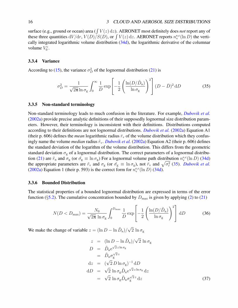
3.3.4 Variance
According to (15), the variance σ2D of the lognormal distribution (21) is
σ2D =
1√2π lnσg
∫ ∞0
1
Dexp
−1
2
(ln(D/Dn)
lnσg
)2 (D − D)2 dD (35)
3.3.5 Non-standard terminology
Non-standard terminology leads to much confusion in the literature. For example, Dubovik et al.(2002a) provide precise analytic definitions of their supposedly lognormal size distribution param-eters. However, their terminology is inconsistent with their definitions. Distributions computedaccording to their definitions are not lognormal distributions. Dubovik et al. (2002a) Equation A1(their p. 606) defines the mean logarithmic radius rv of the volume distribution which they confus-ingly name the volume median radius rv. Dubovik et al. (2002a) Equation A2 (their p. 606) definesthe standard deviation of the logarithm of the volume distribution. This differs from the geometricstandard deviation σg of a lognormal distribution. The correct parameters of a lognormal distribu-tion (21) are rn and σg (or σg ≡ lnσg) For a lognormal volume path distribution ne,c
v (lnD) (34d)the appropriate parameters are rv and σg (or σg ≡ lnσg), not rv and
√σ2r (35). Dubovik et al.
(2002a) Equation 1 (their p. 593) is the correct form for ne,cv (lnD) (34d).
3.3.6 Bounded Distribution
The statistical properties of a bounded lognormal distribution are expressed in terms of the errorfunction (§5.2). The cumulative concentration bounded by Dmax is given by applying (2) to (21)
N(D < Dmax) =N0√
2π lnσg
∫ Dmax
0
1
Dexp
−1
2
(ln(D/Dn)
lnσg
)2 dD (36)
We make the change of variable z = (lnD − ln Dn)/√
2 ln σg
z = (lnD − ln Dn)/√
2 ln σg
D = Dne√
2 z lnσg
= Dnσ√
2 zg
dz = (√
2D lnσg)−1 dD
dD =√
2 ln σgDne√
2 z lnσg dz
=√
2 ln σgDnσ√
2 zg dz (37)
3.3 Lognormal Distribution 17
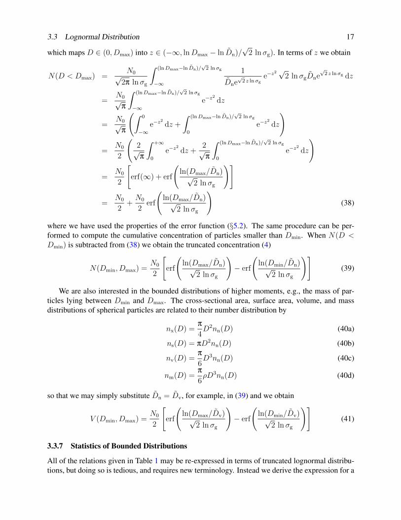
which maps D ∈ (0, Dmax) into z ∈ (−∞, lnDmax − ln Dn)/√
2 lnσg). In terms of z we obtain
N(D < Dmax) =N0√
2π lnσg
∫ (lnDmax−ln Dn)/√
2 lnσg
−∞
1
Dne√
2 z lnσge−z
2 √2 lnσgDne
√2 z lnσg dz
=N0√
π
∫ (lnDmax−ln Dn)/√
2 lnσg
−∞e−z
2
dz
=N0√
π
(∫ 0
−∞e−z
2
dz +
∫ (lnDmax−ln Dn)/√
2 lnσg
0
e−z2
dz
)
=N0
2
(2√π
∫ +∞
0
e−z2
dz +2√π
∫ (lnDmax−ln Dn)/√
2 lnσg
0
e−z2
dz
)
=N0
2
[erf(∞) + erf
(ln(Dmax/Dn)√
2 ln σg
)]
=N0
2+N0
2erf
(ln(Dmax/Dn)√
2 ln σg
)(38)
where we have used the properties of the error function (§5.2). The same procedure can be per-formed to compute the cumulative concentration of particles smaller than Dmin. When N(D <Dmin) is subtracted from (38) we obtain the truncated concentration (4)
N(Dmin, Dmax) =N0
2
[erf
(ln(Dmax/Dn)√
2 ln σg
)− erf
(ln(Dmin/Dn)√
2 ln σg
)](39)
We are also interested in the bounded distributions of higher moments, e.g., the mass of par-ticles lying between Dmin and Dmax. The cross-sectional area, surface area, volume, and massdistributions of spherical particles are related to their number distribution by
nx(D) =π
4D2nn(D) (40a)
ns(D) = πD2nn(D) (40b)
nv(D) =π
6D3nn(D) (40c)
nm(D) =π
6ρD3nn(D) (40d)
so that we may simply substitute Dn = Dv, for example, in (39) and we obtain
V (Dmin, Dmax) =N0
2
[erf
(ln(Dmax/Dv)√
2 lnσg
)− erf
(ln(Dmin/Dv)√
2 lnσg
)](41)
3.3.7 Statistics of Bounded Distributions
All of the relations given in Table 1 may be re-expressed in terms of truncated lognormal distribu-tions, but doing so is tedious, and requires new terminology. Instead we derive the expression for a
18 3 CLOUD AND AEROSOL SIZE DISTRIBUTIONS
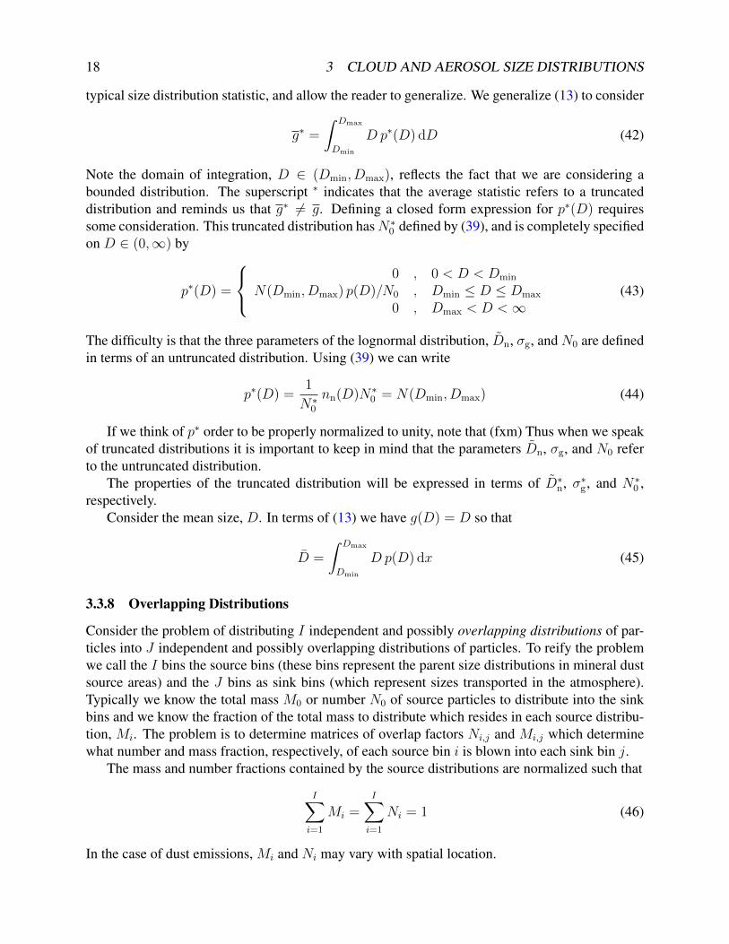
typical size distribution statistic, and allow the reader to generalize. We generalize (13) to consider
g∗ =
∫ Dmax
Dmin
Dp∗(D) dD (42)
Note the domain of integration, D ∈ (Dmin, Dmax), reflects the fact that we are considering abounded distribution. The superscript ∗ indicates that the average statistic refers to a truncateddistribution and reminds us that g∗ 6= g. Defining a closed form expression for p∗(D) requiressome consideration. This truncated distribution hasN∗0 defined by (39), and is completely specifiedon D ∈ (0,∞) by
p∗(D) =
0 , 0 < D < Dmin
N(Dmin, Dmax) p(D)/N0 , Dmin ≤ D ≤ Dmax
0 , Dmax < D <∞(43)
The difficulty is that the three parameters of the lognormal distribution, Dn, σg, and N0 are definedin terms of an untruncated distribution. Using (39) we can write
p∗(D) =1
N∗0nn(D)N∗0 = N(Dmin, Dmax) (44)
If we think of p∗ order to be properly normalized to unity, note that (fxm) Thus when we speakof truncated distributions it is important to keep in mind that the parameters Dn, σg, and N0 referto the untruncated distribution.
The properties of the truncated distribution will be expressed in terms of D∗n, σ∗g , and N∗0 ,respectively.
Consider the mean size, D. In terms of (13) we have g(D) = D so that
D =
∫ Dmax
Dmin
Dp(D) dx (45)
3.3.8 Overlapping Distributions
Consider the problem of distributing I independent and possibly overlapping distributions of par-ticles into J independent and possibly overlapping distributions of particles. To reify the problemwe call the I bins the source bins (these bins represent the parent size distributions in mineral dustsource areas) and the J bins as sink bins (which represent sizes transported in the atmosphere).Typically we know the total mass M0 or number N0 of source particles to distribute into the sinkbins and we know the fraction of the total mass to distribute which resides in each source distribu-tion, Mi. The problem is to determine matrices of overlap factors Ni,j and Mi,j which determinewhat number and mass fraction, respectively, of each source bin i is blown into each sink bin j.
The mass and number fractions contained by the source distributions are normalized such that
I∑i=1
Mi =I∑i=1
Ni = 1 (46)
In the case of dust emissions, Mi and Ni may vary with spatial location.
3.3 Lognormal Distribution 19
The overlap factors Ni,j and Mi,j are defined by the relations
Nj =I∑i=1
Ni,jNi
= N0
I∑i=1
Ni,jNi (47)
Mj =I∑i=1
Mi,jMi
= M0
I∑i=1
Mi,jMi (48)
Using (39) and (46) we find
Ni,j =1
2
[erf
(ln(Dmax,j/Dn,i)√
2 ln σg,i
)− erf
(ln(Dmin,j/Dn,i)√
2 ln σg,i
)](49)
Mi,j =1
2
[erf
(ln(Dmax,j/Dv,i)√
2 lnσg,i
)− erf
(ln(Dmin,j/Dv,i)√
2 lnσg,i
)](50)
fxm: The mathematical derivation appears correct but the overlap factor appears to asymptote to0.5 rather than to 1.0 for Dmax � Dn � Dmin.
A mass distribution has the same form as a lognormal number distribution but has a differentmedian diameter. Thus the overlap matrix elements apply equally to mass and number distributionsdepending on the median diameter used in the following formulae. For the case where both sourceand sink distributions are complete lognormal distributions,
M(D) =i=I∑i=1
Mi(D)
3.3.9 Median Diameter
Substituting D = Dn into (38) we obtain
N(D < Dn) =N0
2(51)
This proves that Dn is the median diameter (5). The lognormal distribution is the only distributionknown (to us) which is most naturally expressed in terms of its median diameter.
3.3.10 Mode Diameter
The mode is the most frequently occuring value of a distribution. The mode diameter or modaldiameter of the number distribution nn(D) is the diameter Dn that satisfies
dnn(D)
dD
∣∣∣∣D=Dn
= 0 (52)
20 3 CLOUD AND AEROSOL SIZE DISTRIBUTIONS
Applying condition (52) to (21) proves that the median and modal diameters are identical forlognormal distributions
Dn = Dn (53)
The number, surface, volume, and mass distributions are all lognormal if any one is. Therefore(53) implies Ds = Ds, and Dv = Dv.
3.3.11 Multimodal Distributions
Realistic particle size distributions may be expressed as an appropriately weighted sum of individ-ual modes.
nn(D) =I∑i=1
nin(D) (54)
where nin(D) is the number distribution of the ith component mode19. Such particle size distribu-tions are called multimodal istributions because they contain one maximum for each componentdistribution. Generalizing (1), the total number concentration becomes
N0 =I∑i=1
∫ ∞0
nin(D) dD
=I∑i=1
N i0 (55)
where N i0 is the total number concentration of the ith component mode.
The median diameter of a multimodal distribution is obtained by following the logic of (36)–(39). The number of particles smaller than a given size is
N(D < Dmax) =I∑i=1
N i0
2+N i
0
2erf
(ln(Dmax/D
in)√
2 ln σig
)(56)
(57)
For the median particle size, Dmax ≡ Dn, and we can move the unknown Dn to the LHS yielding
I∑i=1
N i0
2+N i
0
2erf
(ln(Dn/D
in)√
2 ln σig
)=
N0
2
I∑i=1
N i0 erf
(ln(Dn/D
in)√
2 ln σig
)= 0 (58)
where we have used N0 =∑I
i Ni0. Obtaining Dn for a multimodal distribution requires numeri-
cally solving (58) given the N i0, Di
n, and σig.
19Throughout this section the i superscript represents an index of the component mode, not an exponent.
3.4 Higher Moments 21
3.4 Higher MomentsIt is often useful to compute higher moments of the number distribution. Each factor of the inde-pendent variable weighting the number distribution function nn(D) in the integrand of (14) countsas a moment. The kth moment of nn(D) is
F (k) =
∫ ∞0
nn(D)Dk dD (59)
The statistical properties of higher moments of the lognormal size distribution may be obtainedby direct integration of (59).
F (k) =N0√
2π lnσg
∫ ∞0
1
Dexp
−1
2
(ln(D/Dn)
lnσg
)2Dk dD
=N0√
2π lnσg
∫ ∞0
Dk−1 exp
−1
2
(ln(D/Dn)
lnσg
)2 dD (60)
We make the same change of variable z = (lnD − ln Dn)/√
2 ln σg as in (37). This maps D ∈(0,+∞) into z ∈ (−∞,+∞). In terms of z we obtain
F (k) =N0√
2π lnσg
∫ +∞
−∞(Dne
√2 z lnσg)k−1e−z
2√2 ln σgDne
√2 z lnσg dz
=N0√
π
∫ +∞
−∞(Dne
√2 z lnσg)ke−z
2
dz
=N0D
kn√
π
∫ +∞
−∞e√
2kz lnσge−z2
dz
=N0D
kn√
π
∫ +∞
−∞e−z
2+√
2kz lnσg dz
=N0D
kn√
π
√π exp
(2k2 ln2 σg
4
)= N0D
kn exp(1
2k2 ln2 σg) (61)
where we have used (74) with α = 1 and β =√
2k lnσg.Applying the formula (61) to the first five moments of the lognormal distribution function we
obtain
F (0) =
∫ ∞0
nn(D) dD = N0 = N0 = N0
F (1) =
∫ ∞0
nn(D)D dD = N0Dn exp(12
ln2 σg) = D0 = N0Dn
F (2) =
∫ ∞0
nn(D)D2 dD = N0D2n exp(2 ln2 σg) =
S0
π= N0D
2s
F (3) =
∫ ∞0
nn(D)D3 dD = N0D3n exp(9
2ln2 σg) =
6V0
π= N0D
3v
F (4) =
∫ ∞0
nn(D)D4 dD = N0D4n exp(8 ln2 σg)
(62)
22 3 CLOUD AND AEROSOL SIZE DISTRIBUTIONS
Table 1 includes these relations appear in slightly different forms.The first few moments of the number distribution are related to measurable properties of the
size distribution. In particular, F (k = 0) is the number concentration. Other quantities of meritare ratios of consecutive moments. For example, the volume-weighted diameter Dv is computedby weighted each diameter by the volume of particles at that diameter and then normalizing by thetotal volume of all particles.
Dv =
∫ ∞0
Dπ
6D3nn(D) dD
/∫ ∞0
π
6D3nn(D) dD
=
∫ ∞0
D4nn(D) dD
/∫ ∞0
D3nn(D) dD
= F (4)/F (3)
=N0D
4n exp(8 ln2 σg)
N0D3n exp(9
2ln2 σg)
= Dn exp(72
ln2 σg) (63)
The surface-weighted diameter Ds is defined analogously to Dv. Ds is more often known byits other name, the effective diameter (twice the effective radius). The term “effective” refers tothe light extinction properties of the distribution. Light impinging on a particle distribution is, inthe limit of geometric optics, extinguished in proportion to the cross-sectional area of the particles.Hence the effective diameter (or radius) characterizes the extinction properties of the distribution.Following (63), the effective diameter is
Ds = F (3)/F (2)
=N0D
3n exp(9
2ln2 σg)
N0D2n exp(2 ln2 σg)
= Dn exp(52
ln2 σg) (64)
Moment-weighted diameters, such as the volume-weighted diameter Dv (63), characterize dis-perse distributions. A disperse mass distribution nm(D) behaves most like a monodisperse dis-tribution with all mass residing at D = Dv. Due to approximations, physical operators maybe constrained to act on a single, representative diameter rather than an entire distribution. The“least-wrong” diameter to pick is the moment-weighted diameter most relevant to the process be-ing modeled. For example, Dv best represents the gravitational sedimentation of a distribution ofparticles. On the other hand, Ds (64) best represents the scattering cross-section of a distributionof particles.
3.4.1 Aspherical Particles
The useful relation (??) is a property of the lognormal distribution itself, rather than the particleshape. A lognormal distribution of aspherical particles also obeys (??). Important measurableproperties of most convex aspherical habits may be represented by a constant times the kth momentF (k) of the distribution. For example, the surface area Sh [m2] and volume Vh [m3] of hexagonalprisms are given by (??)–(??). To be consistent with the diameter-centric expressions in Table 1,
3.4 Higher Moments 23
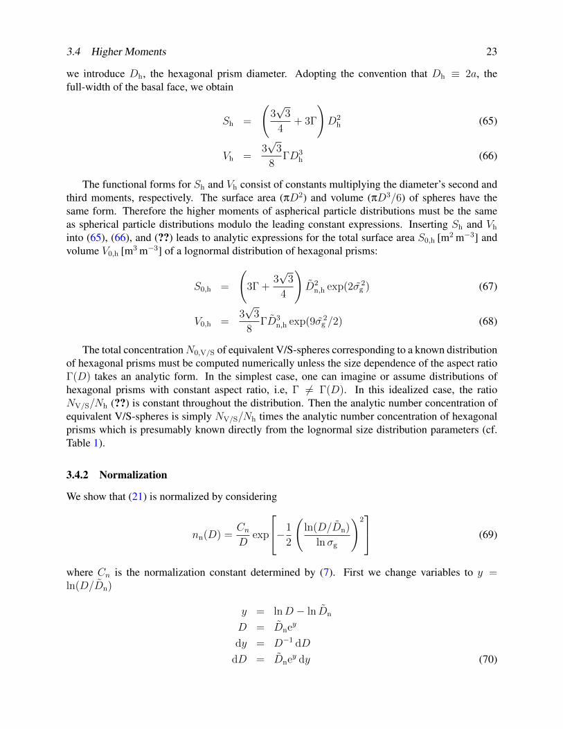
we introduce Dh, the hexagonal prism diameter. Adopting the convention that Dh ≡ 2a, thefull-width of the basal face, we obtain
Sh =
(3√
3
4+ 3Γ
)D2
h (65)
Vh =3√
3
8ΓD3
h (66)
The functional forms for Sh and Vh consist of constants multiplying the diameter’s second andthird moments, respectively. The surface area (πD2) and volume (πD3/6) of spheres have thesame form. Therefore the higher moments of aspherical particle distributions must be the sameas spherical particle distributions modulo the leading constant expressions. Inserting Sh and Vh
into (65), (66), and (??) leads to analytic expressions for the total surface area S0,h [m2 m−3] andvolume V0,h [m3 m−3] of a lognormal distribution of hexagonal prisms:
S0,h =
(3Γ +
3√
3
4
)D2
n,h exp(2σg2) (67)
V0,h =3√
3
8ΓD3
n,h exp(9σg2/2) (68)
The total concentrationN0,V/S of equivalent V/S-spheres corresponding to a known distributionof hexagonal prisms must be computed numerically unless the size dependence of the aspect ratioΓ(D) takes an analytic form. In the simplest case, one can imagine or assume distributions ofhexagonal prisms with constant aspect ratio, i.e, Γ 6= Γ(D). In this idealized case, the ratioNV/S/Nh (??) is constant throughout the distribution. Then the analytic number concentration ofequivalent V/S-spheres is simply NV/S/Nh times the analytic number concentration of hexagonalprisms which is presumably known directly from the lognormal size distribution parameters (cf.Table 1).
3.4.2 Normalization
We show that (21) is normalized by considering
nn(D) =CnD
exp
−1
2
(ln(D/Dn)
lnσg
)2 (69)
where Cn is the normalization constant determined by (7). First we change variables to y =ln(D/Dn)
y = lnD − ln Dn
D = Dney
dy = D−1 dD
dD = Dney dy (70)
24 4 IMPLEMENTATION IN NCAR MODELS
This transformation maps D ∈ (0,+∞) into y ∈ (−∞,+∞). In terms of y, the normalizationcondition (7) becomes∫ +∞
−∞
Cn
Dn exp yexp
[−1
2
(y
lnσg
)2]Dn expy dy = 1
∫ +∞
−∞Cn exp
[−1
2
(y
lnσg
)2]
dy = 1
Next we change variables to z = y/ lnσg
z = y/ lnσg
y = z lnσg
dz = (lnσg)−1 dy
dy = lnσg dz (71)
This transformation does not change the limits of integration and we obtain∫ +∞
−∞Cn exp
(−z2
2
)lnσg dz = 1
Cn√
2π lnσg = 1
Cn =1√
2π lnσg
(72)
In the above we used the well-known normalization property of the Gaussian distribution function,∫ +∞−∞ e−x
2/2 dx =√
2π (73).
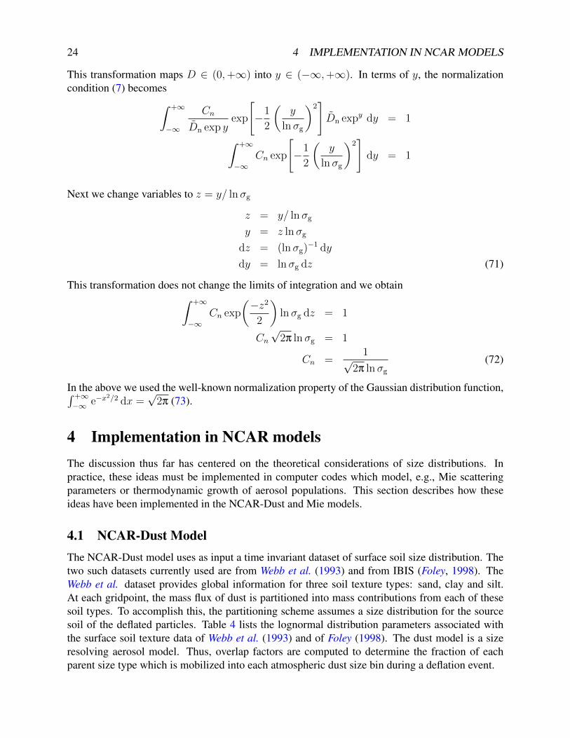
4 Implementation in NCAR modelsThe discussion thus far has centered on the theoretical considerations of size distributions. Inpractice, these ideas must be implemented in computer codes which model, e.g., Mie scatteringparameters or thermodynamic growth of aerosol populations. This section describes how theseideas have been implemented in the NCAR-Dust and Mie models.
4.1 NCAR-Dust ModelThe NCAR-Dust model uses as input a time invariant dataset of surface soil size distribution. Thetwo such datasets currently used are from Webb et al. (1993) and from IBIS (Foley, 1998). TheWebb et al. dataset provides global information for three soil texture types: sand, clay and silt.At each gridpoint, the mass flux of dust is partitioned into mass contributions from each of thesesoil types. To accomplish this, the partitioning scheme assumes a size distribution for the sourcesoil of the deflated particles. Table 4 lists the lognormal distribution parameters associated withthe surface soil texture data of Webb et al. (1993) and of Foley (1998). The dust model is a sizeresolving aerosol model. Thus, overlap factors are computed to determine the fraction of eachparent size type which is mobilized into each atmospheric dust size bin during a deflation event.
4.1 NCAR-Dust Model 25
Soil Texture Dn σg Description
Sand SandSilt SiltClay Clay
Soil Texture Dn σg DescriptionSand SandSilt SiltClay Clay
Table 4: Source size distribution associated with surface soil texture data of Webb et al. (1993) andof Foley (1998).
26 4 IMPLEMENTATION IN NCAR MODELS
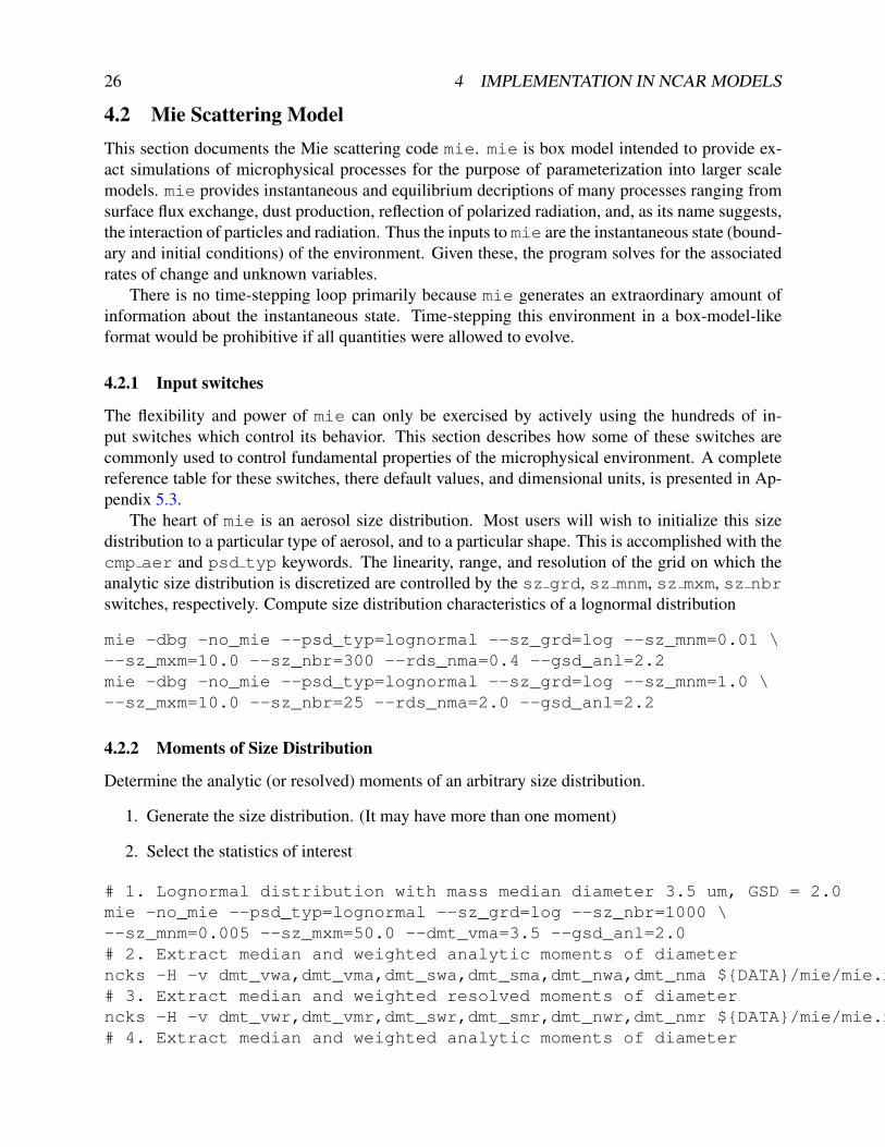
4.2 Mie Scattering ModelThis section documents the Mie scattering code mie. mie is box model intended to provide ex-act simulations of microphysical processes for the purpose of parameterization into larger scalemodels. mie provides instantaneous and equilibrium decriptions of many processes ranging fromsurface flux exchange, dust production, reflection of polarized radiation, and, as its name suggests,the interaction of particles and radiation. Thus the inputs to mie are the instantaneous state (bound-ary and initial conditions) of the environment. Given these, the program solves for the associatedrates of change and unknown variables.
There is no time-stepping loop primarily because mie generates an extraordinary amount ofinformation about the instantaneous state. Time-stepping this environment in a box-model-likeformat would be prohibitive if all quantities were allowed to evolve.
4.2.1 Input switches
The flexibility and power of mie can only be exercised by actively using the hundreds of in-put switches which control its behavior. This section describes how some of these switches arecommonly used to control fundamental properties of the microphysical environment. A completereference table for these switches, there default values, and dimensional units, is presented in Ap-pendix 5.3.
The heart of mie is an aerosol size distribution. Most users will wish to initialize this sizedistribution to a particular type of aerosol, and to a particular shape. This is accomplished with thecmp aer and psd typ keywords. The linearity, range, and resolution of the grid on which theanalytic size distribution is discretized are controlled by the sz grd, sz mnm, sz mxm, sz nbrswitches, respectively. Compute size distribution characteristics of a lognormal distribution
mie -dbg -no_mie --psd_typ=lognormal --sz_grd=log --sz_mnm=0.01 \--sz_mxm=10.0 --sz_nbr=300 --rds_nma=0.4 --gsd_anl=2.2mie -dbg -no_mie --psd_typ=lognormal --sz_grd=log --sz_mnm=1.0 \--sz_mxm=10.0 --sz_nbr=25 --rds_nma=2.0 --gsd_anl=2.2
4.2.2 Moments of Size Distribution
Determine the analytic (or resolved) moments of an arbitrary size distribution.
1. Generate the size distribution. (It may have more than one moment)
2. Select the statistics of interest
# 1. Lognormal distribution with mass median diameter 3.5 um, GSD = 2.0mie -no_mie --psd_typ=lognormal --sz_grd=log --sz_nbr=1000 \--sz_mnm=0.005 --sz_mxm=50.0 --dmt_vma=3.5 --gsd_anl=2.0# 2. Extract median and weighted analytic moments of diameterncks -H -v dmt_vwa,dmt_vma,dmt_swa,dmt_sma,dmt_nwa,dmt_nma ${DATA}/mie/mie.nc# 3. Extract median and weighted resolved moments of diameterncks -H -v dmt_vwr,dmt_vmr,dmt_swr,dmt_smr,dmt_nwr,dmt_nmr ${DATA}/mie/mie.nc# 4. Extract median and weighted analytic moments of diameter
27
ncks -H -v rds_vwa,rds_vma,rds_swa,rds_sma,rds_nwa,rds_nma ${DATA}/mie/mie.nc# 5. Extract median and weighted resolved moments of diameterncks -H -v rds_vwr,rds_vmr,rds_swr,rds_smr,rds_nwr,rds_nmr ${DATA}/mie/mie.nc# 6. Extract number, surface area, and volume distributions at specific sizesncks -H -C -F -u -v dst,dst_rds,dst_sfc,dst_vlm -d sz,1.0e-6 ${DATA}/mie/mie.nc
4.2.3 Generating Properties for Multi-Bin
On occasion, a seriouly masochistic scientist will decide to create the ultimate hybrid bin-spectralaerosol method by discretizing the size distribution into a finite number of bins each with an inde-pendently configurable analytic sub-bin distribution. Generating properties for all the bins in sucha scheme requires enormous amounts of bookkeeping, or, if a computer is available, a relativelysimple Perl batch script named psd.pl.
The psd.pl batch script calls mie repeatedly in a loop over particle bin. As input, psd.placcepts concise array representations of each property of a bin. For example, --sz_nbr={200,25,25,25}specifies that bin 1 is discretized into 200 sub-bins, and the remaining three bins are each dis-cretized into only 25 sub-bins.
˜/dst/psd.pl --dbg=1 --CCM_SW --ftn_fxd --psd_nbr=4 --spc_idx_sng={01,02,03,04} \--sz_mnm={0.05,0.5,1.25,2.5} --sz_mxm={0.5,1.25,2.5,5.0} --sz_nbr={200,25,25,25} \--dmt_vma_dfl=3.5 > ${DATA}/dst/mie/psd_CCM_SW.txt.v3 2>&1 &
5 Appendix
5.1 Properties of GaussiansThe area under a Gaussian distribution may be expressed in closed form for infinite domains.This result can be obtained (IIRC) by transforming to polar coordinates in the complex planex = r(cos θ + i sin θ). ∫ +∞
−∞e−x
2/2 dx =√
2π (73)
This is a special case of a more general result∫ +∞
−∞exp(−αx2 − βx) dx =
√π
αexp
(β2
4α
)where α > 0 (74)
To obtain this result, complete the square under the integrand, change variables to y = x + β/2α,and then apply (73). Substituting α = 1/2 and β = 0 into (74) yields (73).
5.2 Error FunctionThe error function erf(x) may be defined as the partial integral of a Gaussian curve
erf(z) =2√π
∫ z
0
e−x2
dx (75)
28 5 APPENDIX
Using (73) and the symmetry of a Gaussian curve, it is simple to show that the error function isbounded by the limits erf(0) = 0 and erf(∞) = 1. Thus erf(z) is the cumulative probability func-tion for a normally distributed variable z (fxm: True??). Most compilers implement erf(x) as anintrinsic function. Thus erf(x) is used to compute areas bounded by finite lognormal distributions(§3.3.6).
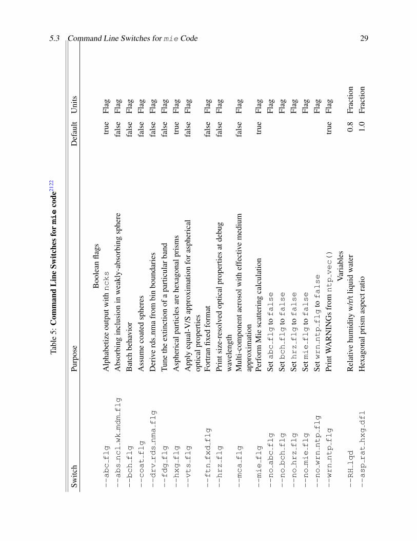
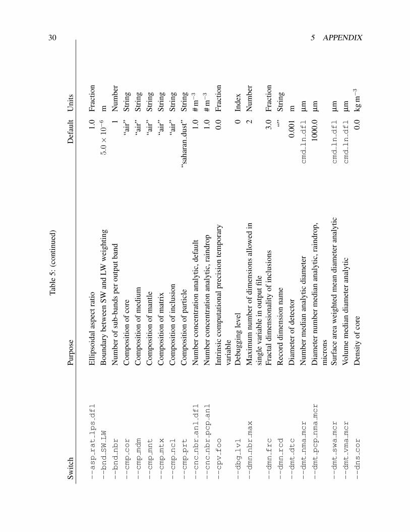
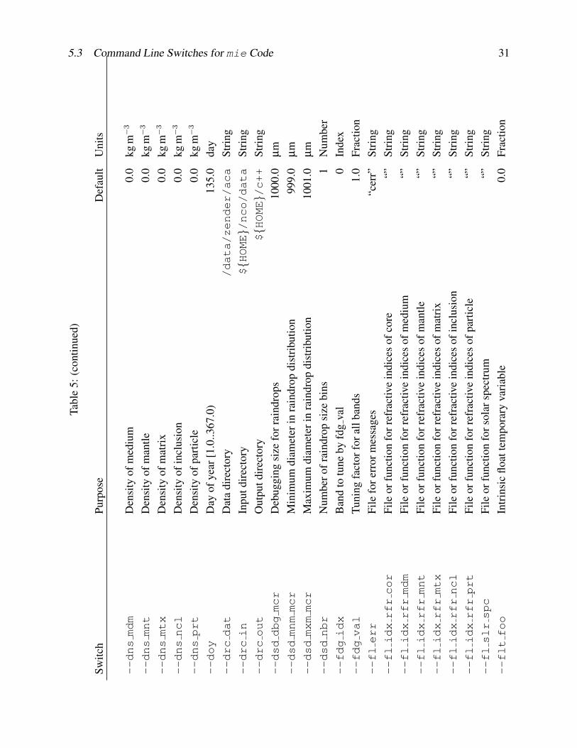
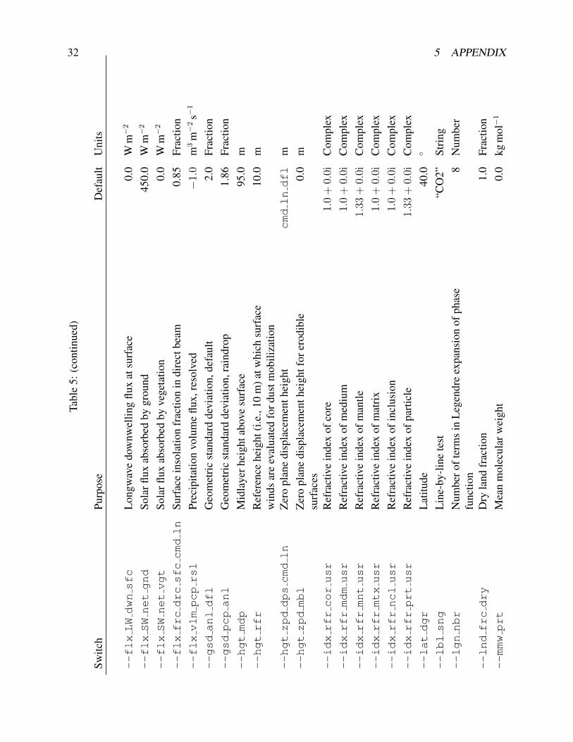
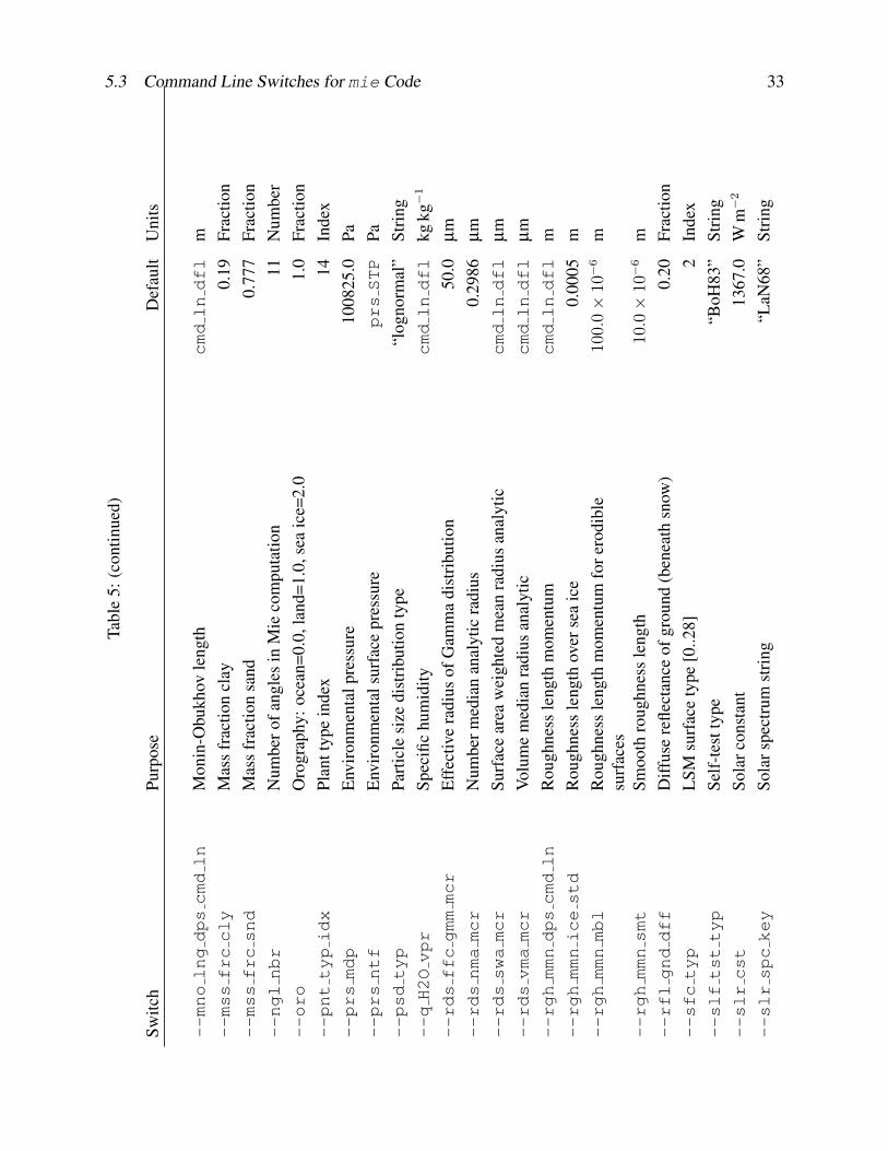
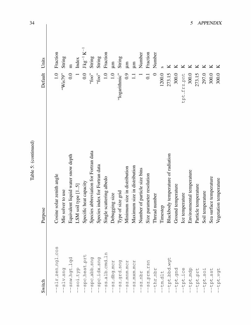
5.3 Command Line Switches for mie CodeTable 5 summarizes all of the command line arguments available to control the behavior of the mieprogram. This is a summary only—it is impractical to think that written documentation could everyconvey the exact meaning of all the switches20. The most frequently used switches are describedin Section 4.2.1. The only way to learn the full meaning of the more obscure switches is to readthe source code itself.
20Perhaps the most useful way to begin to contribute to this FACT would be to systematize and extend the docu-mentation of command line switches
5.3 Command Line Switches for mie Code 29
Tabl
e5:
Com
man
dL
ine
Switc
hesf
ormie
code
2122
Switc
hPu
rpos
eD
efau
ltU
nits
Boo
lean
flags
--abcflg
Alp
habe
tize
outp
utw
ithncks
true
Flag
--absnclwkmdmflg
Abs
orbi
ngin
clus
ion
inw
eakl
y-ab
sorb
ing
sphe
refa
lse
Flag
--bchflg
Bat
chbe
havi
orfa
lse
Flag
--coatflg
Ass
ume
coat
edsp
here
sfa
lse
Flag
--drvrdsnmaflg
Der
ive
rds
nma
from
bin
boun
dari
esfa
lse
Flag
--fdgflg
Tune
the
extin
ctio
nof
apa
rtic
ular
band
fals
eFl
ag--hxgflg
Asp
heri
calp
artic
les
are
hexa
gona
lpri
sms
true
Flag
--vtsflg
App
lyeq
ual-
V/S
appr
oxim
atio
nfo
rasp
heri
cal
optic
alpr
oper
ties
fals
eFl
ag
--ftnfxdflg
Fort
ran
fixed
form
atfa
lse
Flag
--hrzflg
Prin
tsiz
e-re
solv
edop
tical
prop
ertie
sat
debu
gw
avel
engt
hfa
lse
Flag
--mcaflg
Mul
ti-co
mpo
nent
aero
solw
ithef
fect
ive
med
ium
appr
oxim
atio
nfa
lse
Flag
--mieflg
Perf
orm
Mie
scat
teri
ngca
lcul
atio
ntr
ueFl
ag--noabcflg
Setabcflg
tofalse
Flag
--nobchflg
Setbchflg
tofalse
Flag
--nohrzflg
Sethrzflg
tofalse
Flag
--nomieflg
Setmieflg
tofalse
Flag
--nowrnntpflg
Setwrnntpflg
tofalse
Flag
--wrnntpflg
Prin
tWA
RN
ING
sfr
omntpvec()
true
Flag
Var
iabl
es--RHlqd
Rel
ativ
ehu
mid
ityw
/r/t
liqui
dw
ater
0.8
Frac
tion
--asprathxgdfl
Hex
agon
alpr
ism
aspe
ctra
tio1.
0Fr
actio
n
30 5 APPENDIX
Tabl
e5:
(con
tinue
d)
Switc
hPu
rpos
eD
efau
ltU
nits
--aspratlpsdfl
Elli
psoi
dala
spec
trat
io1.
0Fr
actio
n--bndSWLW
Bou
ndar
ybe
twee
nSW
and
LWw
eigh
ting
5.0×
10−
6m
--bndnbr
Num
bero
fsub
-ban
dspe
rout
putb
and
1N
umbe
r--cmpcor
Com
posi
tion
ofco
re“a
ir”
Stri
ng--cmpmdm
Com
posi
tion
ofm
ediu
m“a
ir”
Stri
ng--cmpmnt
Com
posi
tion
ofm
antle
“air
”St
ring
--cmpmtx
Com
posi
tion
ofm
atri
x“a
ir”
Stri
ng--cmpncl
Com
posi
tion
ofin
clus
ion
“air
”St
ring
--cmpprt
Com
posi
tion
ofpa
rtic
le“s
ahar
andu
st”
Stri
ng--cncnbranldfl
Num
berc
once
ntra
tion
anal
ytic
,def
ault
1.0
#m−
3
--cncnbrpcpanl
Num
berc
once
ntra
tion
anal
ytic
,rai
ndro
p1.
0#
m−
3
--cpvfoo
Intr
insi
cco
mpu
tatio
nalp
reci
sion
tem
pora
ryva
riab
le0.
0Fr
actio
n
--dbglvl
Deb
uggi
ngle
vel
0In
dex
--dmnnbrmax
Max
imum
num
bero
fdim
ensi
ons
allo
wed
insi
ngle
vari
able
inou
tput
file
2N
umbe
r
--dmnfrc
Frac
tald
imen
sion
ality
ofin
clus
ions
3.0
Frac
tion
--dmnrcd
Rec
ord
dim
ensi
onna
me
“”St
ring
--dmtdtc
Dia
met
erof
dete
ctor
0.00
1m
--dmtnmamcr
Num
berm
edia
nan
alyt
icdi
amet
ercmdlndfl
µm
--dmtpcpnmamcr
Dia
met
ernu
mbe
rmed
ian
anal
ytic
,rai
ndro
p,m
icro
ns10
00.0
µm
--dmtswamcr
Surf
ace
area
wei
ghte
dm
ean
diam
eter
anal
ytic
cmdlndfl
µm
--dmtvmamcr
Volu
me
med
ian
diam
eter
anal
ytic
cmdlndfl
µm
--dnscor
Den
sity
ofco
re0.
0kg
m−
3
5.3 Command Line Switches for mie Code 31
Tabl
e5:
(con
tinue
d)
Switc
hPu
rpos
eD
efau
ltU
nits
--dnsmdm
Den
sity
ofm
ediu
m0.
0kg
m−
3
--dnsmnt
Den
sity
ofm
antle
0.0
kgm−
3
--dnsmtx
Den
sity
ofm
atri
x0.
0kg
m−
3
--dnsncl
Den
sity
ofin
clus
ion
0.0
kgm−
3
--dnsprt
Den
sity
ofpa
rtic
le0.
0kg
m−
3
--doy
Day
ofye
ar[1
.0..3
67.0
)13
5.0
day
--drcdat
Dat
adi
rect
ory
/data/zender/aca
Stri
ng--drcin
Inpu
tdir
ecto
ry${HOME}/nco/data
Stri
ng--drcout
Out
putd
irec
tory
${HOME}/c++
Stri
ng--dsddbgmcr
Deb
uggi
ngsi
zefo
rrai
ndro
ps10
00.0
µm
--dsdmnmmcr
Min
imum
diam
eter
inra
indr
opdi
stri
butio
n99
9.0
µm
--dsdmxmmcr
Max
imum
diam
eter
inra
indr
opdi
stri
butio
n10
01.0
µm
--dsdnbr
Num
bero
frai
ndro
psi
zebi
ns1
Num
ber
--fdgidx
Ban
dto
tune
byfd
gva
l0
Inde
x--fdgval
Tuni
ngfa
ctor
fora
llba
nds
1.0
Frac
tion
--flerr
File
fore
rror
mes
sage
s“c
err”
Stri
ng--flidxrfrcor
File
orfu
nctio
nfo
rref
ract
ive
indi
ces
ofco
re“”
Stri
ng--flidxrfrmdm
File
orfu
nctio
nfo
rref
ract
ive
indi
ces
ofm
ediu
m“”
Stri
ng--flidxrfrmnt
File
orfu
nctio
nfo
rref
ract
ive
indi
ces
ofm
antle
“”St
ring
--flidxrfrmtx
File
orfu
nctio
nfo
rref
ract
ive
indi
ces
ofm
atri
x“”
Stri
ng--flidxrfrncl
File
orfu
nctio
nfo
rref
ract
ive
indi
ces
ofin
clus
ion
“”St
ring
--flidxrfrprt
File
orfu
nctio
nfo
rref
ract
ive
indi
ces
ofpa
rtic
le“”
Stri
ng--flslrspc
File
orfu
nctio
nfo
rsol
arsp
ectr
um“”
Stri
ng--fltfoo
Intr
insi
cflo
atte
mpo
rary
vari
able
0.0
Frac
tion
32 5 APPENDIX
Tabl
e5:
(con
tinue
d)
Switc
hPu
rpos
eD
efau
ltU
nits
--flxLWdwnsfc
Lon
gwav
edo
wnw
ellin
gflu
xat
surf
ace
0.0
Wm−
2
--flxSWnetgnd
Sola
rflux
abso
rbed
bygr
ound
450.
0W
m−
2
--flxSWnetvgt
Sola
rflux
abso
rbed
byve
geta
tion
0.0
Wm−
2
--flxfrcdrcsfccmdln
Surf
ace
inso
latio
nfr
actio
nin
dire
ctbe
am0.
85Fr
actio
n--flxvlmpcprsl
Prec
ipita
tion
volu
me
flux,
reso
lved
−1.
0m
3m−
2s−
1
--gsdanldfl
Geo
met
ric
stan
dard
devi
atio
n,de
faul
t2.
0Fr
actio
n--gsdpcpanl
Geo
met
ric
stan
dard
devi
atio
n,ra
indr
op1.
86Fr
actio
n--hgtmdp
Mid
laye
rhei
ghta
bove
surf
ace
95.0
m--hgtrfr
Ref
eren
cehe
ight
(i.e
.,10
m)a
twhi
chsu
rfac
ew
inds
are
eval
uate
dfo
rdus
tmob
iliza
tion
10.0
m
--hgtzpddpscmdln
Zer
opl
ane
disp
lace
men
thei
ght
cmdlndfl
m--hgtzpdmbl
Zer
opl
ane
disp
lace
men
thei
ghtf
orer
odib
lesu
rfac
es0.
0m
--idxrfrcorusr
Ref
ract
ive
inde
xof
core
1.0
+0.
0iC
ompl
ex--idxrfrmdmusr
Ref
ract
ive
inde
xof
med
ium
1.0
+0.
0iC
ompl
ex--idxrfrmntusr
Ref
ract
ive
inde
xof
man
tle1.
33+
0.0i
Com
plex
--idxrfrmtxusr
Ref
ract
ive
inde
xof
mat
rix
1.0
+0.
0iC
ompl
ex--idxrfrnclusr
Ref
ract
ive
inde
xof
incl
usio
n1.
0+
0.0i
Com
plex
--idxrfrprtusr
Ref
ract
ive
inde
xof
part
icle
1.33
+0.
0iC
ompl
ex--latdgr
Lat
itude
40.0
◦
--lblsng
Lin
e-by
-lin
ete
st“C
O2”
Stri
ng--lgnnbr
Num
bero
fter
ms
inL
egen
dre
expa
nsio
nof
phas
efu
nctio
n8
Num
ber
--lndfrcdry
Dry
land
frac
tion
1.0
Frac
tion
--mmwprt
Mea
nm
olec
ular
wei
ght
0.0
kgm
ol−
1
5.3 Command Line Switches for mie Code 33
Tabl
e5:
(con
tinue
d)
Switc
hPu
rpos
eD
efau
ltU
nits
--mnolngdpscmdln
Mon
in-O
bukh
ovle
ngth
cmdlndfl
m--mssfrccly
Mas
sfr
actio
ncl
ay0.
19Fr
actio
n--mssfrcsnd
Mas
sfr
actio
nsa
nd0.
777
Frac
tion
--nglnbr
Num
bero
fang
les
inM
ieco
mpu
tatio
n11
Num
ber
--oro
Oro
grap
hy:o
cean
=0.0
,lan
d=1.
0,se
aic
e=2.
01.
0Fr
actio
n--pnttypidx
Plan
ttyp
ein
dex
14In
dex
--prsmdp
Env
iron
men
talp
ress
ure
1008
25.0
Pa--prsntf
Env
iron
men
tals
urfa
cepr
essu
reprsSTP
Pa--psdtyp
Part
icle
size
dist
ribu
tion
type
“log
norm
al”
Stri
ng--qH2Ovpr
Spec
ific
hum
idity
cmdlndfl
kgkg−
1
--rdsffcgmmmcr
Eff
ectiv
era
dius
ofG
amm
adi
stri
butio
n50
.0µ
m--rdsnmamcr
Num
berm
edia
nan
alyt
icra
dius
0.29
86µ
m--rdsswamcr
Surf
ace
area
wei
ghte
dm
ean
radi
usan
alyt
iccmdlndfl
µm
--rdsvmamcr
Volu
me
med
ian
radi
usan
alyt
iccmdlndfl
µm
--rghmmndpscmdln
Rou
ghne
ssle
ngth
mom
entu
mcmdlndfl
m--rghmmnicestd
Rou
ghne
ssle
ngth
over
sea
ice
0.00
05m
--rghmmnmbl
Rou
ghne
ssle
ngth
mom
entu
mfo
rero
dibl
esu
rfac
es10
0.0×
10−
6m
--rghmmnsmt
Smoo
thro
ughn
ess
leng
th10.0×
10−
6m
--rflgnddff
Diff
use
refle
ctan
ceof
grou
nd(b
enea
thsn
ow)
0.20
Frac
tion
--sfctyp
LSM
surf
ace
type
[0..2
8]2
Inde
x--slftsttyp
Self
-tes
ttyp
e“B
oH83
”St
ring
--slrcst
Sola
rcon
stan
t13
67.0
Wm−
2
--slrspckey
Sola
rspe
ctru
mst
ring
“LaN
68”
Stri
ng
34 5 APPENDIX
Tabl
e5:
(con
tinue
d)
Switc
hPu
rpos
eD
efau
ltU
nits
--slrzennglcos
Cos
ine
sola
rzen
ithan
gle
1.0
Frac
tion
--slvsng
Mie
solv
erto
use
“Wis
79”
Stri
ng--snwhgtlqd
Equ
ival
entl
iqui
dw
ater
snow
dept
h0.
0m
--soityp
LSM
soil
type
[1..5
]1
Inde
x--spcheatprt
Spec
ific
heat
capa
city
0.0
Jkg−
1K−
1
--spcabbsng
Spec
ies
abbr
evia
tion
forF
ortr
anda
ta“f
oo”
Stri
ng--spcidxsng
Spec
ies
inde
xfo
rFor
tran
data
“foo
”St
ring
--ssalbcmdln
Sing
lesc
atte
ring
albe
do1.
0Fr
actio
n--szdbgmcr
Deb
uggi
ngsi
ze1.
0µ
m--szgrdsng
Type
ofsi
zegr
id“l
ogar
ithm
ic”
Stri
ng--szmnmmcr
Min
imum
size
indi
stri
butio
n0.
9µ
m--szmxmmcr
Max
imum
size
indi
stri
butio
n1.
1µ
m--sznbr
Num
bero
fpar
ticle
size
bins
1N
umbe
r--szprmrsn
Size
para
met
erre
solu
tion
0.1
Frac
tion
--thrnbr
Thr
ead
num
ber
0N
umbe
r--tmdlt
Tim
este
p12
00.0
s--tptbbdwgt
Bla
ckbo
dyte
mpe
ratu
reof
radi
atio
n27
3.15
K--tptgnd
Gro
und
tem
pera
ture
300.
0K
--tptice
Ice
tem
pera
ture
tptfrzpnt
K--tptmdp
Env
iron
men
talt
empe
ratu
re30
0.0
K--tptprt
Part
icle
tem
pera
ture
273.
15K
--tptsoi
Soil
tem
pera
ture
297.
0K
--tptsst
Sea
surf
ace
tem
pera
ture
300.
0K
--tptvgt
Veg
etat
ion
tem
pera
ture
300.
0K
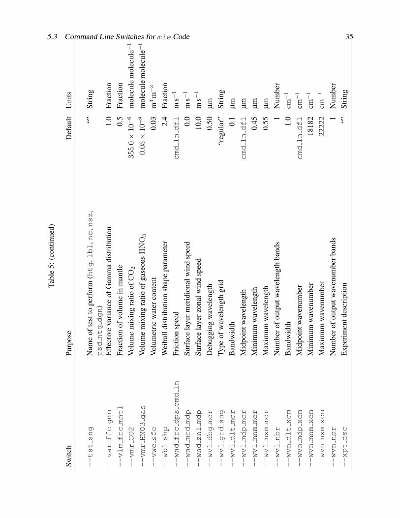
5.3 Command Line Switches for mie Code 35
Tabl
e5:
(con
tinue
d)
Switc
hPu
rpos
eD
efau
ltU
nits
--tstsng
Nam
eof
test
tope
rfor
m(htg
,lbl
,nc
,nsz
,psdntgdgn
)“”
Stri
ng
--varffcgmm
Eff
ectiv
eva
rian
ceof
Gam
ma
dist
ribu
tion
1.0
Frac
tion
--vlmfrcmntl
Frac
tion
ofvo
lum
ein
man
tle0.
5Fr
actio
n--vmrCO2
Volu
me
mix
ing
ratio
ofC
O2
355.
0×
10−
6m
olec
ule
mol
ecul
e−1
--vmrHNO3gas
Volu
me
mix
ing
ratio
ofga
seou
sH
NO
30.
05×
10−
9m
olec
ule
mol
ecul
e−1
--vwcsfc
Volu
met
ric
wat
erco
nten
t0.
03m
3m−
3
--wblshp
Wei
bull
dist
ribu
tion
shap
epa
ram
eter
2.4
Frac
tion
--wndfrcdpscmdln
Fric
tion
spee
dcmdlndfl
ms−
1
--wndmrdmdp
Surf
ace
laye
rmer
idio
nalw
ind
spee
d0.
0m
s−1
--wndznlmdp
Surf
ace
laye
rzon
alw
ind
spee
d10
.0m
s−1
--wvldbgmcr
Deb
uggi
ngw
avel
engt
h0.
50µ
m--wvlgrdsng
Type
ofw
avel
engt
hgr
id“r
egul
ar”
Stri
ng--wvldltmcr
Ban
dwid
th0.
1µ
m--wvlmdpmcr
Mid
poin
twav
elen
gth
cmdlndfl
µm
--wvlmnmmcr
Min
imum
wav
elen
gth
0.45
µm
--wvlmxmmcr
Max
imum
wav
elen
gth
0.55
µm
--wvlnbr
Num
bero
fout
putw
avel
engt
hba
nds
1N
umbe
r--wvndltxcm
Ban
dwid
th1.
0cm−
1
--wvnmdpxcm
Mid
poin
twav
enum
ber
cmdlndfl
cm−
1
--wvnmnmxcm
Min
imum
wav
enum
ber
1818
2cm−
1
--wvnmxmxcm
Max
imum
wav
enum
ber
2222
2cm−
1
--wvnnbr
Num
bero
fout
putw
aven
umbe
rban
ds1
Num
ber
--xptdsc
Exp
erim
entd
escr
iptio
n“”
Stri
ng

36 5 APPENDIX
Table 6 summarizes the fields output by SWNB.
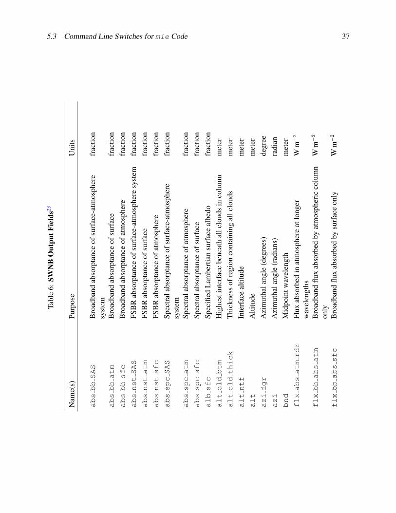
5.3 Command Line Switches for mie Code 37
Tabl
e6:
SWN
BO
utpu
tFie
lds23
Nam
e(s)
Purp
ose
Uni
ts
absbbSAS
Bro
adba
ndab
sorp
tanc
eof
surf
ace-
atm
osph
ere
syst
emfr
actio
n
absbbatm
Bro
adba
ndab
sorp
tanc
eof
surf
ace
frac
tion
absbbsfc
Bro
adba
ndab
sorp
tanc
eof
atm
osph
ere
frac
tion
absnstSAS
FSB
Rab
sorp
tanc
eof
surf
ace-
atm
osph
ere
syst
emfr
actio
nabsnstatm
FSB
Rab
sorp
tanc
eof
surf
ace
frac
tion
absnstsfc
FSB
Rab
sorp
tanc
eof
atm
osph
ere
frac
tion
absspcSAS
Spec
tral
abso
rpta
nce
ofsu
rfac
e-at
mos
pher
esy
stem
frac
tion
absspcatm
Spec
tral
abso
rpta
nce
ofat
mos
pher
efr
actio
nabsspcsfc
Spec
tral
abso
rpta
nce
ofsu
rfac
efr
actio
nalbsfc
Spec
ified
Lam
bert
ian
surf
ace
albe
dofr
actio
naltcldbtm
Hig
hest
inte
rfac
ebe
neat
hal
lclo
uds
inco
lum
nm
eter
altcldthick
Thi
ckne
ssof
regi
onco
ntai
ning
allc
loud
sm
eter
altntf
Inte
rfac
eal
titud
em
eter
alt
Alti
tude
met
erazidgr
Azi
mut
hala
ngle
(deg
rees
)de
gree
azi
Azi
mut
hala
ngle
(rad
ians
)ra
dian
bnd
Mid
poin
twav
elen
gth
met
erflxabsatmrdr
Flux
abso
rbed
inat
mos
pher
eat
long
erw
avel
engt
hsW
m−
2
flxbbabsatm
Bro
adba
ndflu
xab
sorb
edby
atm
osph
eric
colu
mn
only
Wm−
2
flxbbabssfc
Bro
adba
ndflu
xab
sorb
edby
surf
ace
only
Wm−
2
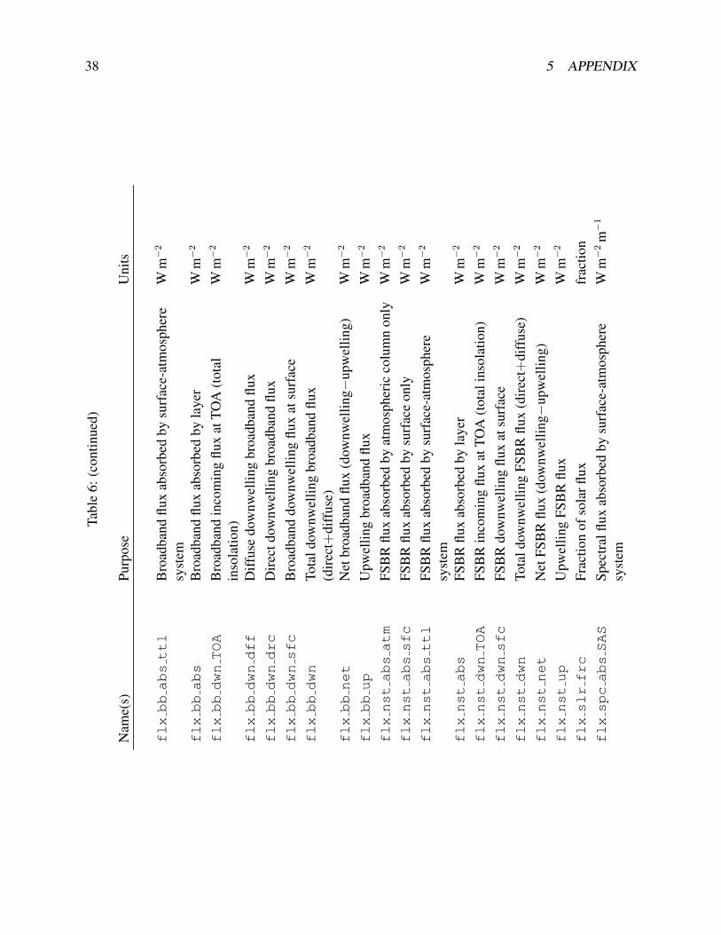
38 5 APPENDIX
Tabl
e6:
(con
tinue
d)
Nam
e(s)
Purp
ose
Uni
ts
flxbbabsttl
Bro
adba
ndflu
xab
sorb
edby
surf
ace-
atm
osph
ere
syst
emW
m−
2
flxbbabs
Bro
adba
ndflu
xab
sorb
edby
laye
rW
m−
2
flxbbdwnTOA
Bro
adba
ndin
com
ing
flux
atTO
A(t
otal
inso
latio
n)W
m−
2
flxbbdwndff
Diff
use
dow
nwel
ling
broa
dban
dflu
xW
m−
2
flxbbdwndrc
Dir
ectd
ownw
ellin
gbr
oadb
and
flux
Wm−
2
flxbbdwnsfc
Bro
adba
nddo
wnw
ellin
gflu
xat
surf
ace
Wm−
2
flxbbdwn
Tota
ldow
nwel
ling
broa
dban
dflu
x(d
irec
t+di
ffus
e)W
m−
2
flxbbnet
Net
broa
dban
dflu
x(d
ownw
ellin
g−up
wel
ling)
Wm−
2
flxbbup
Upw
ellin
gbr
oadb
and
flux
Wm−
2
flxnstabsatm
FSB
Rflu
xab
sorb
edby
atm
osph
eric
colu
mn
only
Wm−
2
flxnstabssfc
FSB
Rflu
xab
sorb
edby
surf
ace
only
Wm−
2
flxnstabsttl
FSB
Rflu
xab
sorb
edby
surf
ace-
atm
osph
ere
syst
emW
m−
2
flxnstabs
FSB
Rflu
xab
sorb
edby
laye
rW
m−
2
flxnstdwnTOA
FSB
Rin
com
ing
flux
atTO
A(t
otal
inso
latio
n)W
m−
2
flxnstdwnsfc
FSB
Rdo
wnw
ellin
gflu
xat
surf
ace
Wm−
2
flxnstdwn
Tota
ldow
nwel
ling
FSB
Rflu
x(d
irec
t+di
ffus
e)W
m−
2
flxnstnet
Net
FSB
Rflu
x(d
ownw
ellin
g−up
wel
ling)
Wm−
2
flxnstup
Upw
ellin
gFS
BR
flux
Wm−
2
flxslrfrc
Frac
tion
ofso
larfl
uxfr
actio
nflxspcabsSAS
Spec
tral
flux
abso
rbed
bysu
rfac
e-at
mos
pher
esy
stem
Wm−
2m−
1
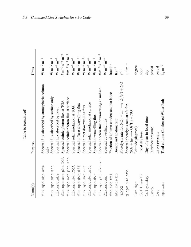
5.3 Command Line Switches for mie Code 39
Tabl
e6:
(con
tinue
d)
Nam
e(s)
Purp
ose
Uni
ts
flxspcabsatm
Spec
tral
flux
abso
rbed
byat
mos
pher
icco
lum
non
lyW
m−
2m−
1
flxspcabssfc
Spec
tral
flux
abso
rbed
bysu
rfac
eon
lyW
m−
2m−
1
flxspcabs
Spec
tral
flux
abso
rbed
byla
yer
Wm−
2m−
1
flxspcactphtTOA
Spec
tral
actin
icph
oton
flux
atTO
A#
m−
2s−
1m−
1
flxspcactphtsfc
Spec
tral
actin
icph
oton
flux
atsu
rfac
e#
m−
2s−
1m−
1
flxspcdwnTOA
Spec
tral
sola
rins
olat
ion
atTO
AW
m−
2m−
1
flxspcdwndff
Spec
tral
diff
use
dow
nwel
ling
flux
Wm−
2m−
1
flxspcdwndrc
Spec
tral
dire
ctdo
wnw
ellin
gflu
xW
m−
2m−
1
flxspcdwnsfc
Spec
tral
sola
rins
olat
ion
atsu
rfac
eW
m−
2m−
1
flxspcdwn
Spec
tral
dow
nwel
ling
flux
Wm−
2m−
1
flxspcphtdwnsfc
Spec
tral
phot
onflu
xdo
wnw
ellin
gat
surf
ace
#m−
2s−
1m−
1
flxspcup
Spec
tral
upw
ellin
gflu
xW
m−
2m−
1
frcicettl
Frac
tion
ofco
lum
nco
nden
sate
that
isic
efr
actio
nhtgratebb
Bro
adba
ndhe
atin
gra
teK
s−1
jNO2
Phot
olys
isra
tefo
rNO
2+
hν−→
O(3
P)
+N
Os−
1
jspcNO2sfc
Spec
tral
phot
olys
isra
teat
sfc
for
NO
2+
hν−→
O(3
P)
+N
Os−
1m−
1
latdgr
Lat
itude
(deg
rees
)de
gree
lcltimehr
Loc
alda
yho
urho
urlclyrday
Day
ofye
arin
loca
ltim
eda
ylevp
Inte
rfac
epr
essu
repa
scal
lev
Lay
erpr
essu
repa
scal
mpcCWP
Tota
lcol
umn
Con
dens
edW
ater
Path
kgm−
2
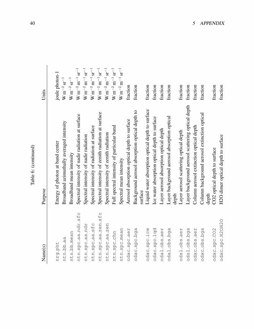
40 5 APPENDIX
Tabl
e6:
(con
tinue
d)
Nam
e(s)
Purp
ose
Uni
ts
nrgpht
Ene
rgy
ofph
oton
atba
ndce
nter
joul
eph
oton
-1ntnbbaa
Bro
adba
ndaz
imut
hally
aver
aged
inte
nsity
Wm−
2sr−
1
ntnbbmean
Bro
adba
ndm
ean
inte
nsity
Wm−
2sr−
1
ntnspcaandrsfc
Spec
tral
inte
nsity
ofna
dirr
adia
tion
atsu
rfac
eW
m−
2m−
1sr−
1
ntnspcaandr
Spec
tral
inte
nsity
ofna
dirr
adia
tion
Wm−
2m−
1sr−
1
ntnspcaasfc
Spec
tral
inte
nsity
ofra
diat
ion
atsu
rfac
eW
m−
2m−
1sr−
1
ntnspcaazensfc
Spec
tral
inte
nsity
ofze
nith
radi
atio
nat
surf
ace
Wm−
2m−
1sr−
1
ntnspcaazen
Spec
tral
inte
nsity
ofze
nith
radi
atio
nW
m−
2m−
1sr−
1
ntnspcchn
Full
spec
tral
inte
nsity
ofpa
rtic
ular
band
Wm−
2m−
1sr−
1
ntnspcmean
Spec
tral
mea
nin
tens
ityW
m−
2m−
1sr−
1
odacspcaer
Aer
osol
abso
rptio
nop
tical
dept
hto
surf
ace
frac
tion
odacspcbga
Bac
kgro
und
aero
sola
bsor
ptio
nop
tical
dept
hto
surf
ace
frac
tion
odacspcice
Liq
uid
wat
erab
sorp
tion
optic
alde
pth
tosu
rfac
efr
actio
nodacspclqd
Ice
wat
erab
sorp
tion
optic
alde
pth
tosu
rfac
efr
actio
nodalobsaer
Lay
erae
roso
labs
orpt
ion
optic
alde
pth
frac
tion
odalobsbga
Lay
erba
ckgr
ound
aero
sola
bsor
ptio
nop
tical
dept
hfr
actio
n
odslobsaer
Lay
erae
roso
lsca
tteri
ngop
tical
dept
hfr
actio
nodslobsbga
Lay
erba
ckgr
ound
aero
sols
catte
ring
optic
alde
pth
frac
tion
odxcobsaer
Col
umn
aero
sole
xtin
ctio
nop
tical
dept
hfr
actio
nodxcobsbga
Col
umn
back
grou
ndae
roso
lext
inct
ion
optic
alde
pth
frac
tion
odxcspcCO2
CO
2op
tical
dept
hto
surf
ace
frac
tion
odxcspcH2OH2O
H2O
dim
erop
tical
dept
hto
surf
ace
frac
tion
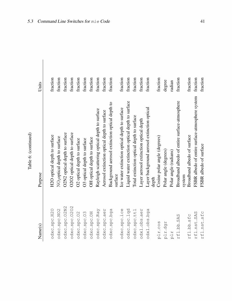
5.3 Command Line Switches for mie Code 41
Tabl
e6:
(con
tinue
d)
Nam
e(s)
Purp
ose
Uni
ts
odxcspcH2O
H2O
optic
alde
pth
tosu
rfac
efr
actio
nodxcspcNO2
NO
2op
tical
dept
hto
surf
ace
frac
tion
odxcspcO2N2
O2N
2op
tical
dept
hto
surf
ace
frac
tion
odxcspcO2O2
O2O
2op
tical
dept
hto
surf
ace
frac
tion
odxcspcO2
O2
optic
alde
pth
tosu
rfac
efr
actio
nodxcspcO3
O3
optic
alde
pth
tosu
rfac
efr
actio
nodxcspcOH
OH
optic
alde
pth
tosu
rfac
efr
actio
nodxcspcRay
Ray
leig
hsc
atte
ring
optic
alde
pth
tosu
rfac
efr
actio
nodxcspcaer
Aer
osol
extin
ctio
nop
tical
dept
hto
surf
ace
frac
tion
odxcspcbga
Bac
kgro
und
aero
sole
xtin
ctio
nop
tical
dept
hto
surf
ace
frac
tion
odxcspcice
Ice
wat
erex
tinct
ion
optic
alde
pth
tosu
rfac
efr
actio
nodxcspclqd
Liq
uid
wat
erex
tinct
ion
optic
alde
pth
tosu
rfac
efr
actio
nodxcspcttl
Tota
lext
inct
ion
optic
alde
pth
tosu
rfac
efr
actio
nodxlobsaer
Lay
erae
roso
lext
inct
ion
optic
alde
pth
frac
tion
odxlobsbga
Lay
erba
ckgr
ound
aero
sole
xtin
ctio
nop
tical
dept
hfr
actio
n
plrcos
Cos
ine
pola
rang
le(d
egre
es)
frac
tion
plrdgr
Pola
rang
le(d
egre
es)
degr
eeplr
Pola
rang
le(r
adia
ns)
radi
anrflbbSAS
Bro
adba
ndal
bedo
ofen
tire
surf
ace-
atm
osph
ere
syst
emfr
actio
n
rflbbsfc
Bro
adba
ndal
bedo
ofsu
rfac
efr
actio
nrflnstSAS
FSB
Ral
bedo
ofen
tire
surf
ace-
atm
osph
ere
syst
emfr
actio
nrflnstsfc
FSB
Ral
bedo
ofsu
rfac
efr
actio
n
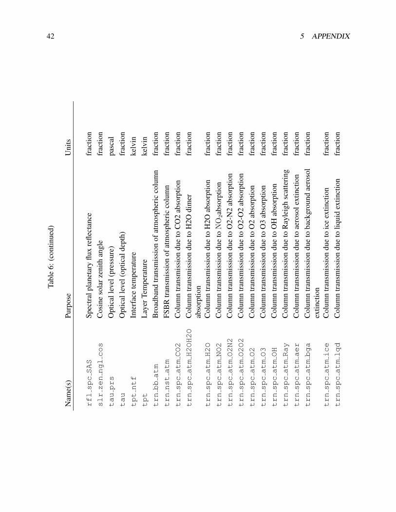
42 5 APPENDIX
Tabl
e6:
(con
tinue
d)
Nam
e(s)
Purp
ose
Uni
ts
rflspcSAS
Spec
tral
plan
etar
yflu
xre
flect
ance
frac
tion
slrzennglcos
Cos
ine
sola
rzen
ithan
gle
frac
tion
tauprs
Opt
ical
leve
l(pr
essu
re)
pasc
altau
Opt
ical
leve
l(op
tical
dept
h)fr
actio
ntptntf
Inte
rfac
ete
mpe
ratu
reke
lvin
tpt
Lay
erTe
mpe
ratu
reke
lvin
trnbbatm
Bro
adba
ndtr
ansm
issi
onof
atm
osph
eric
colu
mn
frac
tion
trnnstatm
FSB
Rtr
ansm
issi
onof
atm
osph
eric
colu
mn
frac
tion
trnspcatmCO2
Col
umn
tran
smis
sion
due
toC
O2
abso
rptio
nfr
actio
ntrnspcatmH2OH2O
Col
umn
tran
smis
sion
due
toH
2Odi
mer
abso
rptio
nfr
actio
n
trnspcatmH2O
Col
umn
tran
smis
sion
due
toH
2Oab
sorp
tion
frac
tion
trnspcatmNO2
Col
umn
tran
smis
sion
due
toN
O2ab
sorp
tion
frac
tion
trnspcatmO2N2
Col
umn
tran
smis
sion
due
toO
2-N
2ab
sorp
tion
frac
tion
trnspcatmO2O2
Col
umn
tran
smis
sion
due
toO
2-O
2ab
sorp
tion
frac
tion
trnspcatmO2
Col
umn
tran
smis
sion
due
toO
2ab
sorp
tion
frac
tion
trnspcatmO3
Col
umn
tran
smis
sion
due
toO
3ab
sorp
tion
frac
tion
trnspcatmOH
Col
umn
tran
smis
sion
due
toO
Hab
sorp
tion
frac
tion
trnspcatmRay
Col
umn
tran
smis
sion
due
toR
ayle
igh
scat
teri
ngfr
actio
ntrnspcatmaer
Col
umn
tran
smis
sion
due
toae
roso
lext
inct
ion
frac
tion
trnspcatmbga
Col
umn
tran
smis
sion
due
toba
ckgr
ound
aero
sol
extin
ctio
nfr
actio
n
trnspcatmice
Col
umn
tran
smis
sion
due
toic
eex
tinct
ion
frac
tion
trnspcatmlqd
Col
umn
tran
smis
sion
due
toliq
uid
extin
ctio
nfr
actio
n
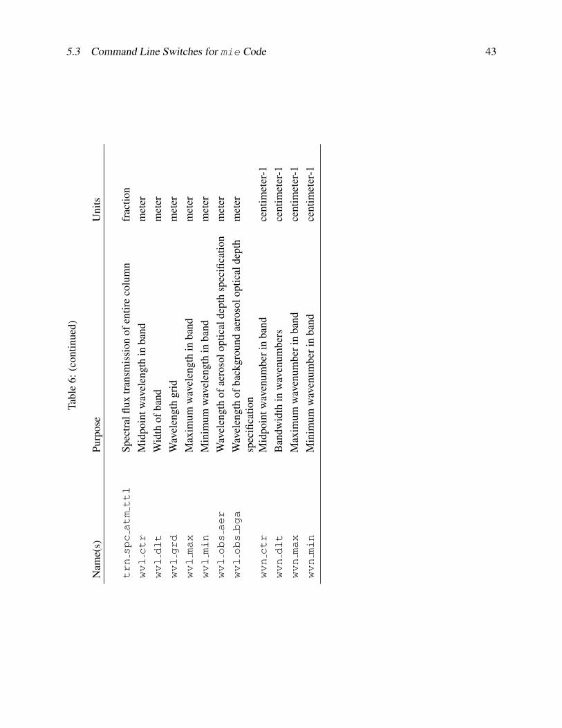
5.3 Command Line Switches for mie Code 43
Tabl
e6:
(con
tinue
d)
Nam
e(s)
Purp
ose
Uni
ts
trnspcatmttl
Spec
tral
flux
tran
smis
sion
ofen
tire
colu
mn
frac
tion
wvlctr
Mid
poin
twav
elen
gth
inba
ndm
eter
wvldlt
Wid
thof
band
met
erwvlgrd
Wav
elen
gth
grid
met
erwvlmax
Max
imum
wav
elen
gth
inba
ndm
eter
wvlmin
Min
imum
wav
elen
gth
inba
ndm
eter
wvlobsaer
Wav
elen
gth
ofae
roso
lopt
ical
dept
hsp
ecifi
catio
nm
eter
wvlobsbga
Wav
elen
gth
ofba
ckgr
ound
aero
solo
ptic
alde
pth
spec
ifica
tion
met
er
wvnctr
Mid
poin
twav
enum
beri
nba
ndce
ntim
eter
-1wvndlt
Ban
dwid
thin
wav
enum
bers
cent
imet
er-1
wvnmax
Max
imum
wav
enum
beri
nba
ndce
ntim
eter
-1wvnmin
Min
imum
wav
enum
beri
nba
ndce
ntim
eter
-1

44 5 APPENDIX
Table 7 summarizes the fields output by CLM.
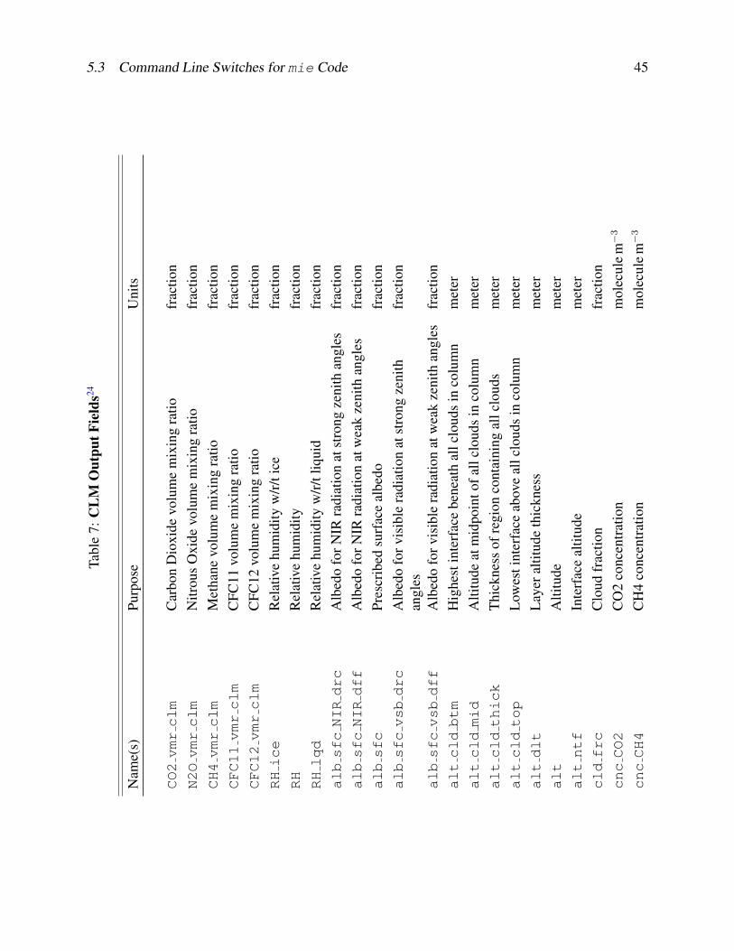
5.3 Command Line Switches for mie Code 45
Tabl
e7:
CL
MO
utpu
tFie
lds24
Nam
e(s)
Purp
ose
Uni
ts
CO2vmrclm
Car
bon
Dio
xide
volu
me
mix
ing
ratio
frac
tion
N2Ovmrclm
Nitr
ous
Oxi
devo
lum
em
ixin
gra
tiofr
actio
nCH4vmrclm
Met
hane
volu
me
mix
ing
ratio
frac
tion
CFC11vmrclm
CFC
11vo
lum
em
ixin
gra
tiofr
actio
nCFC12vmrclm
CFC
12vo
lum
em
ixin
gra
tiofr
actio
nRHice
Rel
ativ
ehu
mid
ityw
/r/t
ice
frac
tion
RH
Rel
ativ
ehu
mid
ityfr
actio
nRHlqd
Rel
ativ
ehu
mid
ityw
/r/t
liqui
dfr
actio
nalbsfcNIRdrc
Alb
edo
forN
IRra
diat
ion
atst
rong
zeni
than
gles
frac
tion
albsfcNIRdff
Alb
edo
forN
IRra
diat
ion
atw
eak
zeni
than
gles
frac
tion
albsfc
Pres
crib
edsu
rfac
eal
bedo
frac
tion
albsfcvsbdrc
Alb
edo
forv
isib
lera
diat
ion
atst
rong
zeni
than
gles
frac
tion
albsfcvsbdff
Alb
edo
forv
isib
lera
diat
ion
atw
eak
zeni
than
gles
frac
tion
altcldbtm
Hig
hest
inte
rfac
ebe
neat
hal
lclo
uds
inco
lum
nm
eter
altcldmid
Alti
tude
atm
idpo
into
fall
clou
dsin
colu
mn
met
eraltcldthick
Thi
ckne
ssof
regi
onco
ntai
ning
allc
loud
sm
eter
altcldtop
Low
esti
nter
face
abov
eal
lclo
uds
inco
lum
nm
eter
altdlt
Lay
eral
titud
eth
ickn
ess
met
eralt
Alti
tude
met
eraltntf
Inte
rfac
eal
titud
em
eter
cldfrc
Clo
udfr
actio
nfr
actio
ncncCO2
CO
2co
ncen
trat
ion
mol
ecul
em−
3
cncCH4
CH
4co
ncen
trat
ion
mol
ecul
em−
3
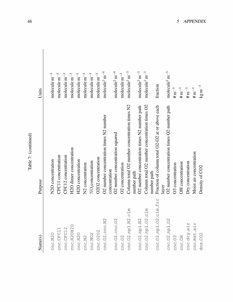
46 5 APPENDIX
Tabl
e7:
(con
tinue
d)
Nam
e(s)
Purp
ose
Uni
ts
cncN2O
N2O
conc
entr
atio
nm
olec
ule
m−
3
cncCFC11
CFC
11co
ncen
trat
ion
mol
ecul
em−
3
cncCFC12
CFC
12co
ncen
trat
ion
mol
ecul
em−
3
cncH2OH2O
H2O
dim
erco
ncen
trat
ion
mol
ecul
em−
3
cncH2O
H2O
conc
entr
atio
nm
olec
ule
m−
3
cncN2
N2
conc
entr
atio
nm
olec
ule
m−
3
cncNO2
NO
2co
ncen
trat
ion
mol
ecul
em−
3
cncO2O2
O2O
2co
ncen
trat
ion
mol
ecul
em−
3
cncO2cncN2
O2
num
berc
once
ntra
tion
times
N2
num
ber
conc
entr
atio
nm
olec
ule2
m−
6
cncO2cncO2
O2
num
berc
once
ntra
tion
squa
red
mol
ecul
e2m−
6
cncO2
O2
conc
entr
atio
nm
olec
ule
m−
3
cncO2nplN2clm
Col
umn
tota
lO2
num
berc
once
ntra
tion
times
N2
num
berp
ath
mol
ecul
e2m−
5
cncO2nplN2
O2
num
berc
once
ntra
tion
times
N2
num
berp
ath
mol
ecul
e2m−
5
cncO2nplO2clm
Col
umn
tota
lO2
num
berc
once
ntra
tion
times
O2
num
berp
ath
mol
ecul
e2m−
5
cncO2nplO2clmfrc
Frac
tion
ofco
lum
nto
talO
2-O
2at
orab
ove
each
laye
rfr
actio
n
cncO2nplO2
O2
num
berc
once
ntra
tion
times
O2
num
berp
ath
mol
ecul
e2m−
5
cncO3
O3
conc
entr
atio
n#
m−
3
cncOH
OH
conc
entr
atio
n#
m−
3
cncdryair
Dry
conc
entr
atio
n#
m−
3
cncmstair
Moi
stai
rcon
cent
ratio
n#
m−
3
dnsCO2
Den
sity
ofC
O2
kgm−
3
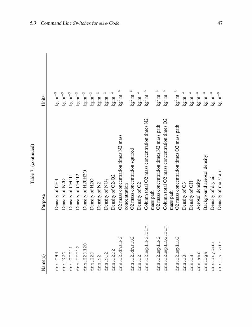
5.3 Command Line Switches for mie Code 47
Tabl
e7:
(con
tinue
d)
Nam
e(s)
Purp
ose
Uni
ts
dnsCH4
Den
sity
ofC
H4
kgm−
3
dnsN2O
Den
sity
ofN
2Okg
m−
3
dnsCFC11
Den
sity
ofC
FC11
kgm−
3
dnsCFC12
Den
sity
ofC
FC12
kgm−
3
dnsH2OH2O
Den
sity
ofH
20H
2Okg
m−
3
dnsH2O
Den
sity
ofH
2Okg
m−
3
dnsN2
Den
sity
ofN
2kg
m−
3
dnsNO2
Den
sity
ofN
O2
kgm−
3
dnsO2O2
Den
sity
ofO
2-O
2kg
m−
3
dnsO2dnsN2
O2
mas
sco
ncen
trat
ion
times
N2
mas
sco
ncen
trat
ion
kg2
m−
6
dnsO2dnsO2
O2
mas
sco
ncen
trat
ion
squa
red
kg2
m−
6
dnsO2
Den
sity
ofO
2kg
m−
3
dnsO2mplN2clm
Col
umn
tota
lO2
mas
sco
ncen
trat
ion
times
N2
mas
spa
thkg
2m−
5
dnsO2mplN2
O2
mas
sco
ncen
trat
ion
times
N2
mas
spa
thkg
2m−
5
dnsO2mplO2clm
Col
umn
tota
lO2
mas
sco
ncen
trat
ion
times
O2
mas
spa
thkg
2m−
5
dnsO2mplO2
O2
mas
sco
ncen
trat
ion
times
O2
mas
spa
thkg
2m−
5
dnsO3
Den
sity
ofO
3kg
m−
3
dnsOH
Den
sity
ofO
Hkg
m−
3
dnsaer
Aer
osol
dens
itykg
m−
3
dnsbga
Bac
kgro
und
aero
sold
ensi
tykg
m−
3
dnsdryair
Den
sity
ofdr
yai
rkg
m−
3
dnsmstair
Den
sity
ofm
oist
air
kgm−
3
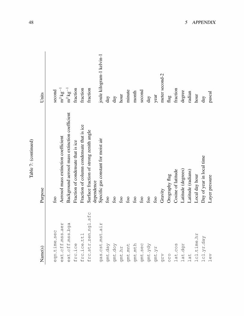
48 5 APPENDIX
Tabl
e7:
(con
tinue
d)
Nam
e(s)
Purp
ose
Uni
ts
eqntimesec
foo
seco
ndextcffmssaer
Aer
osol
mas
sex
tinct
ion
coef
ficie
ntm
2kg−
1
extcffmssbga
Bac
kgro
und
aero
solm
ass
extin
ctio
nco
effic
ient
m2
kg−
1
frcice
Frac
tion
ofco
nden
sate
that
isic
efr
actio
nfrcicettl
Frac
tion
ofco
lum
nco
nden
sate
that
isic
efr
actio
nfrcstrzennglsfc
Surf
ace
frac
tion
ofst
rong
zeni
than
gle
depe
nden
cefr
actio
n
gascstmstair
Spec
ific
gas
cons
tant
form
oist
air
joul
eki
logr
am-1
kelv
in-1
gmtday
foo
day
gmtdoy
foo
day
gmthr
foo
hour
gmtmnt
foo
min
ute
gmtmth
foo
mon
thgmtsec
foo
seco
ndgmtydy
foo
day
gmtyr
foo
year
grv
Gra
vity
met
erse
cond
-2oro
Oro
grap
hyfla
gfla
glatcos
Cos
ine
ofla
titud
efr
actio
nlatdgr
Lat
itude
(deg
rees
)de
gree
lat
Lat
itude
(rad
ians
)ra
dian
lcltimehr
Loc
alda
yho
urho
urlclyrday
Day
ofye
arin
loca
ltim
eda
ylev
Lay
erpr
essu
repa
scal
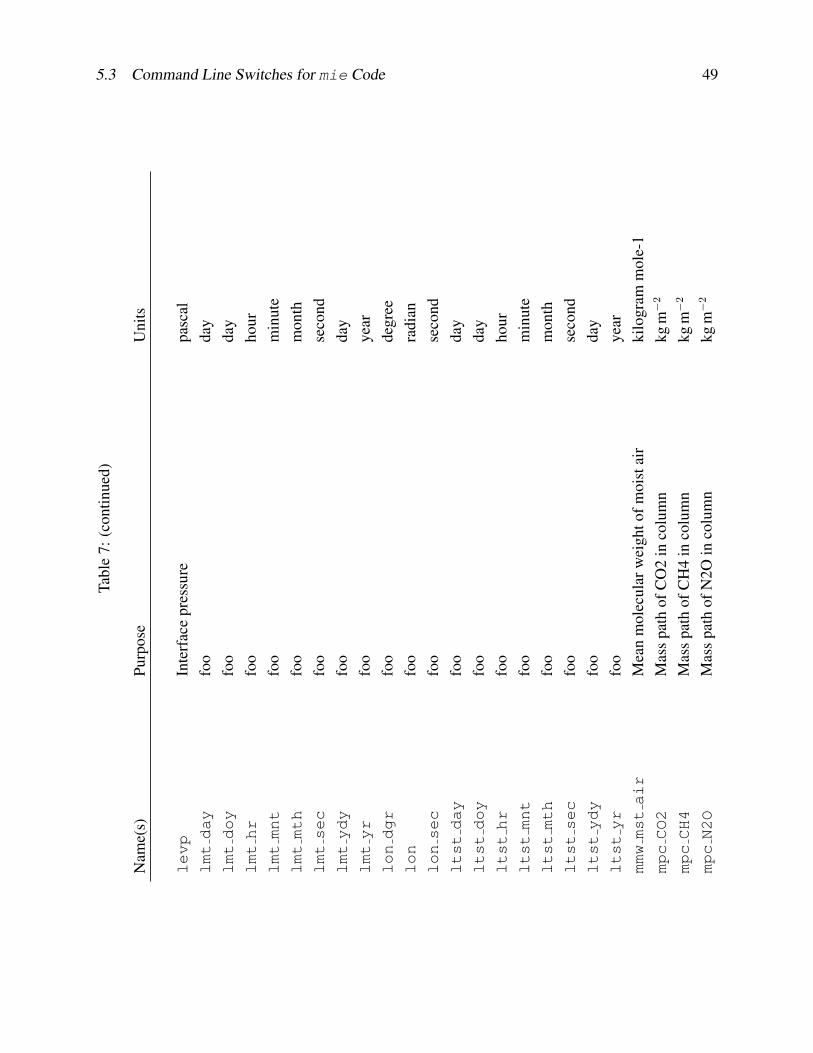
5.3 Command Line Switches for mie Code 49
Tabl
e7:
(con
tinue
d)
Nam
e(s)
Purp
ose
Uni
ts
levp
Inte
rfac
epr
essu
repa
scal
lmtday
foo
day
lmtdoy
foo
day
lmthr
foo
hour
lmtmnt
foo
min
ute
lmtmth
foo
mon
thlmtsec
foo
seco
ndlmtydy
foo
day
lmtyr
foo
year
londgr
foo
degr
eelon
foo
radi
anlonsec
foo
seco
ndltstday
foo
day
ltstdoy
foo
day
ltsthr
foo
hour
ltstmnt
foo
min
ute
ltstmth
foo
mon
thltstsec
foo
seco
ndltstydy
foo
day
ltstyr
foo
year
mmwmstair
Mea
nm
olec
ular
wei
ghto
fmoi
stai
rki
logr
amm
ole-
1mpcCO2
Mas
spa
thof
CO
2in
colu
mn
kgm−
2
mpcCH4
Mas
spa
thof
CH
4in
colu
mn
kgm−
2
mpcN2O
Mas
spa
thof
N2O
inco
lum
nkg
m−
2
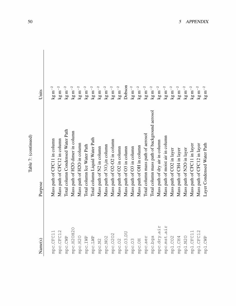
50 5 APPENDIX
Tabl
e7:
(con
tinue
d)
Nam
e(s)
Purp
ose
Uni
ts
mpcCFC11
Mas
spa
thof
CFC
11in
colu
mn
kgm−
2
mpcCFC12
Mas
spa
thof
CFC
12in
colu
mn
kgm−
2
mpcCWP
Tota
lcol
umn
Con
dens
edW
ater
Path
kgm−
2
mpcH2OH2O
Mas
spa
thof
H2O
dim
erin
colu
mn
kgm−
2
mpcH2O
Mas
spa
thof
H2O
inco
lum
nkg
m−
2
mpcIWP
Tota
lcol
umn
Ice
Wat
erPa
thkg
m−
2
mpcLWP
Tota
lcol
umn
Liq
uid
Wat
erPa
thkg
m−
2
mpcN2
Mas
spa
thof
N2
inco
lum
nkg
m−
2
mpcNO2
Mas
spa
thof
NO
2in
colu
mn
kgm−
2
mpcO2O2
Mas
spa
thof
O2-
O2
inco
lum
nkg
m−
2
mpcO2
Mas
spa
thof
O2
inco
lum
nkg
m−
2
mpcO3DU
Mas
spa
thof
O3
inco
lum
nD
obso
nmpcO3
Mas
spa
thof
O3
inco
lum
nkg
m−
2
mpcOH
Mas
spa
thof
OH
inco
lum
nkg
m−
2
mpcaer
Tota
lcol
umn
mas
spa
thof
aero
sol
kgm−
2
mpcbga
Tota
lcol
umn
mas
spa
thof
back
grou
ndae
roso
lkg
m−
2
mpcdryair
Mas
spa
thof
dry
airi
nco
lum
nkg
m−
2
mpcmstair
Mas
spa
thof
moi
stai
rin
colu
mn
kgm−
2
mplCO2
Mas
spa
thof
CO
2in
laye
rkg
m−
2
mplCH4
Mas
spa
thof
CH
4in
laye
rkg
m−
2
mplN2O
Mas
spa
thof
N2O
inla
yer
kgm−
2
mplCFC11
Mas
spa
thof
CFC
11in
laye
rkg
m−
2
mplCFC12
Mas
spa
thof
CFC
12in
laye
rkg
m−
2
mplCWP
Lay
erC
onde
nsed
Wat
erPa
thkg
m−
2
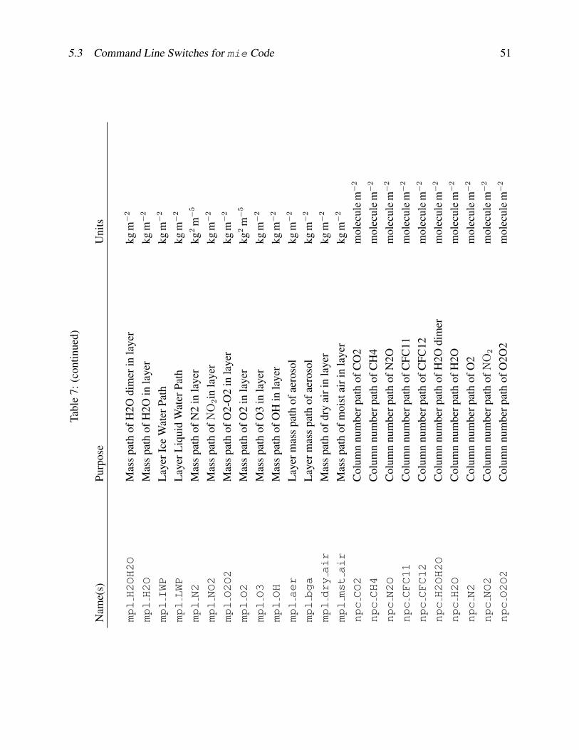
5.3 Command Line Switches for mie Code 51
Tabl
e7:
(con
tinue
d)
Nam
e(s)
Purp
ose
Uni
ts
mplH2OH2O
Mas
spa
thof
H2O
dim
erin
laye
rkg
m−
2
mplH2O
Mas
spa
thof
H2O
inla
yer
kgm−
2
mplIWP
Lay
erIc
eW
ater
Path
kgm−
2
mplLWP
Lay
erL
iqui
dW
ater
Path
kgm−
2
mplN2
Mas
spa
thof
N2
inla
yer
kg2
m−
5
mplNO2
Mas
spa
thof
NO
2in
laye
rkg
m−
2
mplO2O2
Mas
spa
thof
O2-
O2
inla
yer
kgm−
2
mplO2
Mas
spa
thof
O2
inla
yer
kg2
m−
5
mplO3
Mas
spa
thof
O3
inla
yer
kgm−
2
mplOH
Mas
spa
thof
OH
inla
yer
kgm−
2
mplaer
Lay
erm
ass
path
ofae
roso
lkg
m−
2
mplbga
Lay
erm
ass
path
ofae
roso
lkg
m−
2
mpldryair
Mas
spa
thof
dry
airi
nla
yer
kgm−
2
mplmstair
Mas
spa
thof
moi
stai
rin
laye
rkg
m−
2
npcCO2
Col
umn
num
berp
ath
ofC
O2
mol
ecul
em−
2
npcCH4
Col
umn
num
berp
ath
ofC
H4
mol
ecul
em−
2
npcN2O
Col
umn
num
berp
ath
ofN
2Om
olec
ule
m−
2
npcCFC11
Col
umn
num
berp
ath
ofC
FC11
mol
ecul
em−
2
npcCFC12
Col
umn
num
berp
ath
ofC
FC12
mol
ecul
em−
2
npcH2OH2O
Col
umn
num
berp
ath
ofH
2Odi
mer
mol
ecul
em−
2
npcH2O
Col
umn
num
berp
ath
ofH
2Om
olec
ule
m−
2
npcN2
Col
umn
num
berp
ath
ofO
2m
olec
ule
m−
2
npcNO2
Col
umn
num
berp
ath
ofN
O2
mol
ecul
em−
2
npcO2O2
Col
umn
num
berp
ath
ofO
2O2
mol
ecul
em−
2
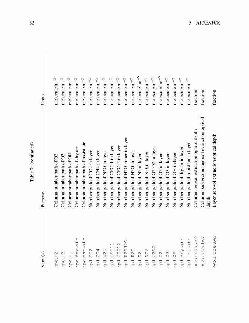
52 5 APPENDIX
Tabl
e7:
(con
tinue
d)
Nam
e(s)
Purp
ose
Uni
ts
npcO2
Col
umn
num
berp
ath
ofO
2m
olec
ule
m−
2
npcO3
Col
umn
num
berp
ath
ofO
3m
olec
ule
m−
2
npcOH
Col
umn
num
berp
ath
ofO
Hm
olec
ule
m−
2
npcdryair
Col
umn
num
berp
ath
ofdr
yai
rm
olec
ule
m−
2
npcmstair
Col
umn
num
berp
ath
ofm
oist
air
mol
ecul
em−
2
nplCO2
Num
berp
ath
ofC
O2
inla
yer
mol
ecul
em−
2
nplCH4
Num
berp
ath
ofC
H4
inla
yer
mol
ecul
em−
2
nplN2O
Num
berp
ath
ofN
2Oin
laye
rm
olec
ule
m−
2
nplCFC11
Num
berp
ath
ofC
FC11
inla
yer
mol
ecul
em−
2
nplCFC12
Num
berp
ath
ofC
FC12
inla
yer
mol
ecul
em−
2
nplH2OH2O
Num
berp
ath
ofH
2Odi
mer
inla
yer
mol
ecul
em−
2
nplH2O
Num
berp
ath
ofH
2Oin
laye
rm
olec
ule
m−
2
nplN2
Num
berp
ath
ofN
2in
laye
rm
olec
ule2
m−
5
nplNO2
Num
berp
ath
ofN
O2in
laye
rm
olec
ule
m−
2
nplO2O2
Num
berp
ath
ofO
2-O
2in
laye
rm
olec
ule
m−
2
nplO2
Num
berp
ath
ofO
2in
laye
rm
olec
ule2
m−
5
nplO3
Num
berp
ath
ofO
3in
laye
rm
olec
ule
m−
2
nplOH
Num
berp
ath
ofO
Hin
laye
rm
olec
ule
m−
2
npldryair
Num
berp
ath
ofdr
yai
rin
laye
rm
olec
ule
m−
2
nplmstair
Num
berp
ath
ofm
oist
airi
nla
yer
mol
ecul
em−
2
odxcobsaer
Col
umn
aero
sole
xtin
ctio
nop
tical
dept
hfr
actio
nodxcobsbga
Col
umn
back
grou
ndae
roso
lext
inct
ion
optic
alde
pth
frac
tion
odxlobsaer
Lay
erae
roso
lext
inct
ion
optic
alde
pth
frac
tion
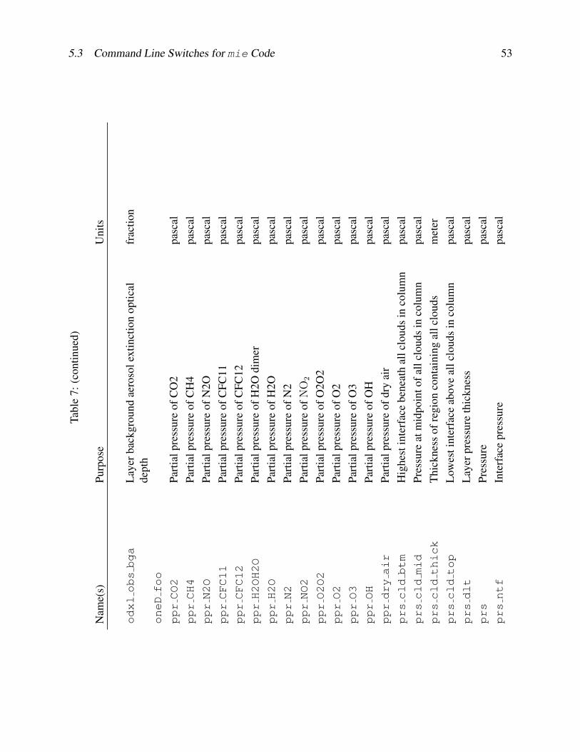
5.3 Command Line Switches for mie Code 53
Tabl
e7:
(con
tinue
d)
Nam
e(s)
Purp
ose
Uni
ts
odxlobsbga
Lay
erba
ckgr
ound
aero
sole
xtin
ctio
nop
tical
dept
hfr
actio
n
oneDfoo
pprCO2
Part
ialp
ress
ure
ofC
O2
pasc
alpprCH4
Part
ialp
ress
ure
ofC
H4
pasc
alpprN2O
Part
ialp
ress
ure
ofN
2Opa
scal
pprCFC11
Part
ialp
ress
ure
ofC
FC11
pasc
alpprCFC12
Part
ialp
ress
ure
ofC
FC12
pasc
alpprH2OH2O
Part
ialp
ress
ure
ofH
2Odi
mer
pasc
alpprH2O
Part
ialp
ress
ure
ofH
2Opa
scal
pprN2
Part
ialp
ress
ure
ofN
2pa
scal
pprNO2
Part
ialp
ress
ure
ofN
O2
pasc
alpprO2O2
Part
ialp
ress
ure
ofO
2O2
pasc
alpprO2
Part
ialp
ress
ure
ofO
2pa
scal
pprO3
Part
ialp
ress
ure
ofO
3pa
scal
pprOH
Part
ialp
ress
ure
ofO
Hpa
scal
pprdryair
Part
ialp
ress
ure
ofdr
yai
rpa
scal
prscldbtm
Hig
hest
inte
rfac
ebe
neat
hal
lclo
uds
inco
lum
npa
scal
prscldmid
Pres
sure
atm
idpo
into
fall
clou
dsin
colu
mn
pasc
alprscldthick
Thi
ckne
ssof
regi
onco
ntai
ning
allc
loud
sm
eter
prscldtop
Low
esti
nter
face
abov
eal
lclo
uds
inco
lum
npa
scal
prsdlt
Lay
erpr
essu
reth
ickn
ess
pasc
alprs
Pres
sure
pasc
alprsntf
Inte
rfac
epr
essu
repa
scal
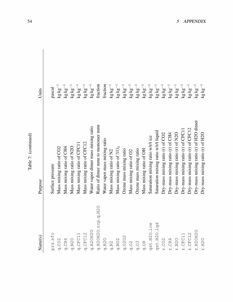
54 5 APPENDIX
Tabl
e7:
(con
tinue
d)
Nam
e(s)
Purp
ose
Uni
ts
prssfc
Surf
ace
pres
sure
pasc
alqCO2
Mas
sm
ixin
gra
tioof
CO
2kg
kg−
1
qCH4
Mas
sm
ixin
gra
tioof
CH
4kg
kg−
1
qN2O
Mas
sm
ixin
gra
tioof
N2O
kgkg−
1
qCFC11
Mas
sm
ixin
gra
tioof
CFC
11kg
kg−
1
qCFC12
Mas
sm
ixin
gra
tioof
CFC
12kg
kg−
1
qH2OH2O
Wat
erva
pord
imer
mas
sm
ixin
gra
tiokg
kg−
1
qH2OH2OrcpqH2O
Rat
ioof
dim
erm
mrt
om
onom
erm
mr
frac
tion
qH2O
Wat
erva
porm
ass
mix
ing
ratio
frac
tion
qN2
Mas
sm
ixin
gra
tioof
N2
kgkg−
1
qNO2
Mas
sm
ixin
gra
tioof
NO
2kg
kg−
1
qO2O2
Ozo
nem
ass
mix
ing
ratio
kgkg−
1
qO2
Mas
sm
ixin
gra
tioof
O2
kgkg−
1
qO3
Ozo
nem
ass
mix
ing
ratio
kgkg−
1
qOH
Mas
sm
ixin
gra
tioof
OH
kgkg−
1
qstH2Oice
Satu
ratio
nm
ixin
gra
tiow
/r/t
ice
kgkg−
1
qstH2Olqd
Satu
ratio
nm
ixin
gra
tiow
/r/t
liqui
dkg
kg−
1
rCO2
Dry
-mas
sm
ixin
gra
tio(r
)ofC
O2
kgkg−
1
rCH4
Dry
-mas
sm
ixin
gra
tio(r
)ofC
H4
kgkg−
1
rN2O
Dry
-mas
sm
ixin
gra
tio(r
)ofN
2Okg
kg−
1
rCFC11
Dry
-mas
sm
ixin
gra
tio(r
)ofC
FC11
kgkg−
1
rCFC12
Dry
-mas
sm
ixin
gra
tio(r
)ofC
FC12
kgkg−
1
rH2OH2O
Dry
-mas
sm
ixin
gra
tio(r
)ofH
2Odi
mer
kgkg−
1
rH2O
Dry
-mas
sm
ixin
gra
tio(r
)ofH
2Okg
kg−
1
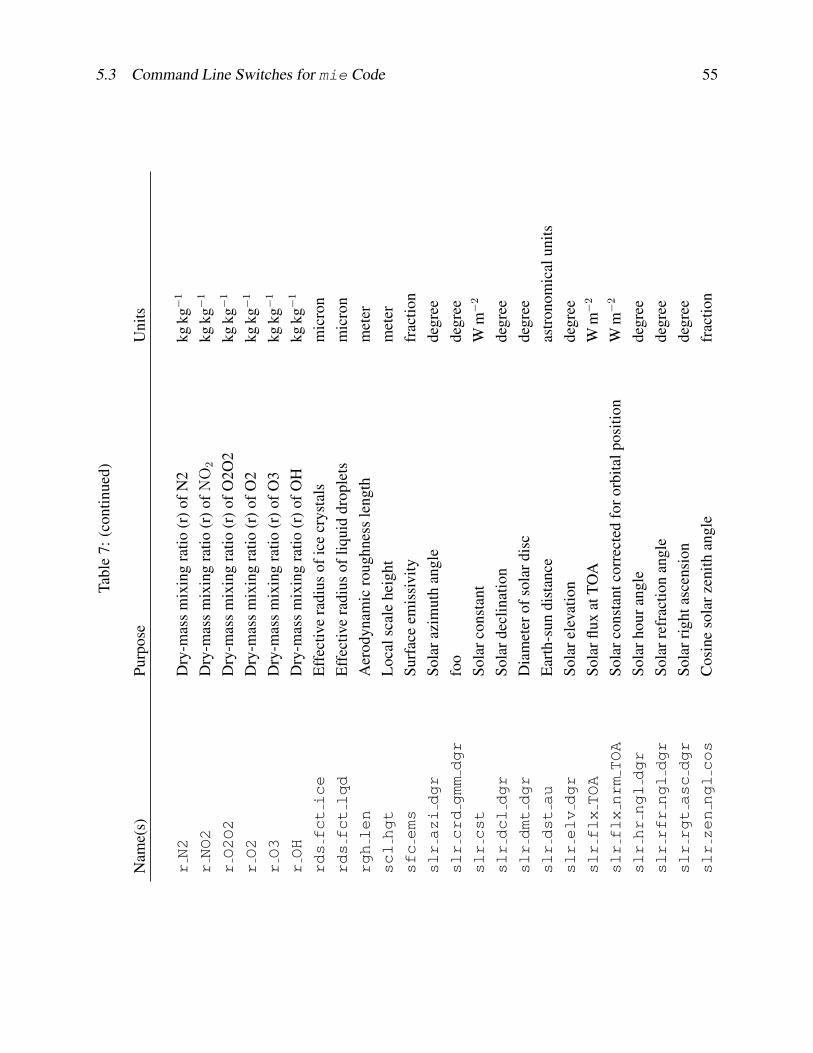
5.3 Command Line Switches for mie Code 55
Tabl
e7:
(con
tinue
d)
Nam
e(s)
Purp
ose
Uni
ts
rN2
Dry
-mas
sm
ixin
gra
tio(r
)ofN
2kg
kg−
1
rNO2
Dry
-mas
sm
ixin
gra
tio(r
)ofN
O2
kgkg−
1
rO2O2
Dry
-mas
sm
ixin
gra
tio(r
)ofO
2O2
kgkg−
1
rO2
Dry
-mas
sm
ixin
gra
tio(r
)ofO
2kg
kg−
1
rO3
Dry
-mas
sm
ixin
gra
tio(r
)ofO
3kg
kg−
1
rOH
Dry
-mas
sm
ixin
gra
tio(r
)ofO
Hkg
kg−
1
rdsfctice
Eff
ectiv
era
dius
ofic
ecr
ysta
lsm
icro
nrdsfctlqd
Eff
ectiv
era
dius
ofliq
uid
drop
lets
mic
ron
rghlen
Aer
odyn
amic
roug
hnes
sle
ngth
met
ersclhgt
Loc
alsc
ale
heig
htm
eter
sfcems
Surf
ace
emis
sivi
tyfr
actio
nslrazidgr
Sola
razi
mut
han
gle
degr
eeslrcrdgmmdgr
foo
degr
eeslrcst
Sola
rcon
stan
tW
m−
2
slrdcldgr
Sola
rdec
linat
ion
degr
eeslrdmtdgr
Dia
met
erof
sola
rdis
cde
gree
slrdstau
Ear
th-s
undi
stan
ceas
tron
omic
alun
itsslrelvdgr
Sola
rele
vatio
nde
gree
slrflxTOA
Sola
rflux
atTO
AW
m−
2
slrflxnrmTOA
Sola
rcon
stan
tcor
rect
edfo
rorb
italp
ositi
onW
m−
2
slrhrngldgr
Sola
rhou
rang
lede
gree
slrrfrngldgr
Sola
rref
ract
ion
angl
ede
gree
slrrgtascdgr
Sola
rrig
htas
cens
ion
degr
eeslrzennglcos
Cos
ine
sola
rzen
ithan
gle
frac
tion
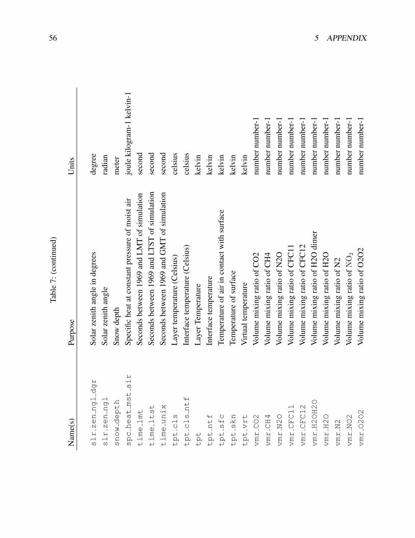
56 5 APPENDIX
Tabl
e7:
(con
tinue
d)
Nam
e(s)
Purp
ose
Uni
ts
slrzenngldgr
Sola
rzen
ithan
gle
inde
gree
sde
gree
slrzenngl
Sola
rzen
ithan
gle
radi
ansnowdepth
Snow
dept
hm
eter
spcheatmstair
Spec
ific
heat
atco
nsta
ntpr
essu
reof
moi
stai
rjo
ule
kilo
gram
-1ke
lvin
-1timelmt
Seco
nds
betw
een
1969
and
LM
Tof
sim
ulat
ion
seco
ndtimeltst
Seco
nds
betw
een
1969
and
LTST
ofsi
mul
atio
nse
cond
timeunix
Seco
nds
betw
een
1969
and
GM
Tof
sim
ulat
ion
seco
ndtptcls
Lay
erte
mpe
ratu
re(C
elsi
us)
cels
ius
tptclsntf
Inte
rfac
ete
mpe
ratu
re(C
elsi
us)
cels
ius
tpt
Lay
erTe
mpe
ratu
reke
lvin
tptntf
Inte
rfac
ete
mpe
ratu
reke
lvin
tptsfc
Tem
pera
ture
ofai
rin
cont
actw
ithsu
rfac
eke
lvin
tptskn
Tem
pera
ture
ofsu
rfac
eke
lvin
tptvrt
Vir
tual
tem
pera
ture
kelv
invmrCO2
Volu
me
mix
ing
ratio
ofC
O2
num
bern
umbe
r-1
vmrCH4
Volu
me
mix
ing
ratio
ofC
H4
num
bern
umbe
r-1
vmrN2O
Volu
me
mix
ing
ratio
ofN
2Onu
mbe
rnum
ber-
1vmrCFC11
Volu
me
mix
ing
ratio
ofC
FC11
num
bern
umbe
r-1
vmrCFC12
Volu
me
mix
ing
ratio
ofC
FC12
num
bern
umbe
r-1
vmrH2OH2O
Volu
me
mix
ing
ratio
ofH
2Odi
mer
num
bern
umbe
r-1
vmrH2O
Volu
me
mix
ing
ratio
ofH
2Onu
mbe
rnum
ber-
1vmrN2
Volu
me
mix
ing
ratio
ofN
2nu
mbe
rnum
ber-
1vmrNO2
Volu
me
mix
ing
ratio
ofN
O2
num
bern
umbe
r-1
vmrO2O2
Volu
me
mix
ing
ratio
ofO
2O2
num
bern
umbe
r-1
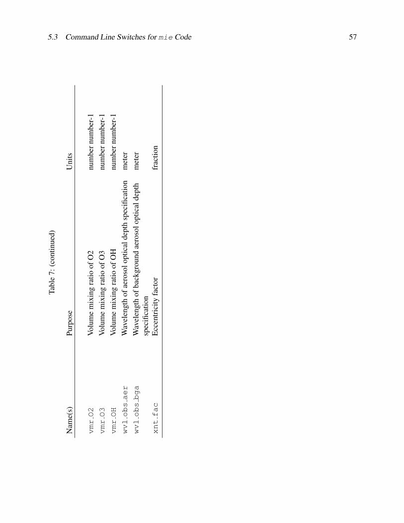
5.3 Command Line Switches for mie Code 57
Tabl
e7:
(con
tinue
d)
Nam
e(s)
Purp
ose
Uni
ts
vmrO2
Volu
me
mix
ing
ratio
ofO
2nu
mbe
rnum
ber-
1vmrO3
Volu
me
mix
ing
ratio
ofO
3nu
mbe
rnum
ber-
1vmrOH
Volu
me
mix
ing
ratio
ofO
Hnu
mbe
rnum
ber-
1wvlobsaer
Wav
elen
gth
ofae
roso
lopt
ical
dept
hsp
ecifi
catio
nm
eter
wvlobsbga
Wav
elen
gth
ofba
ckgr
ound
aero
solo
ptic
alde
pth
spec
ifica
tion
met
er
xntfac
Ecc
entr
icity
fact
orfr
actio
n
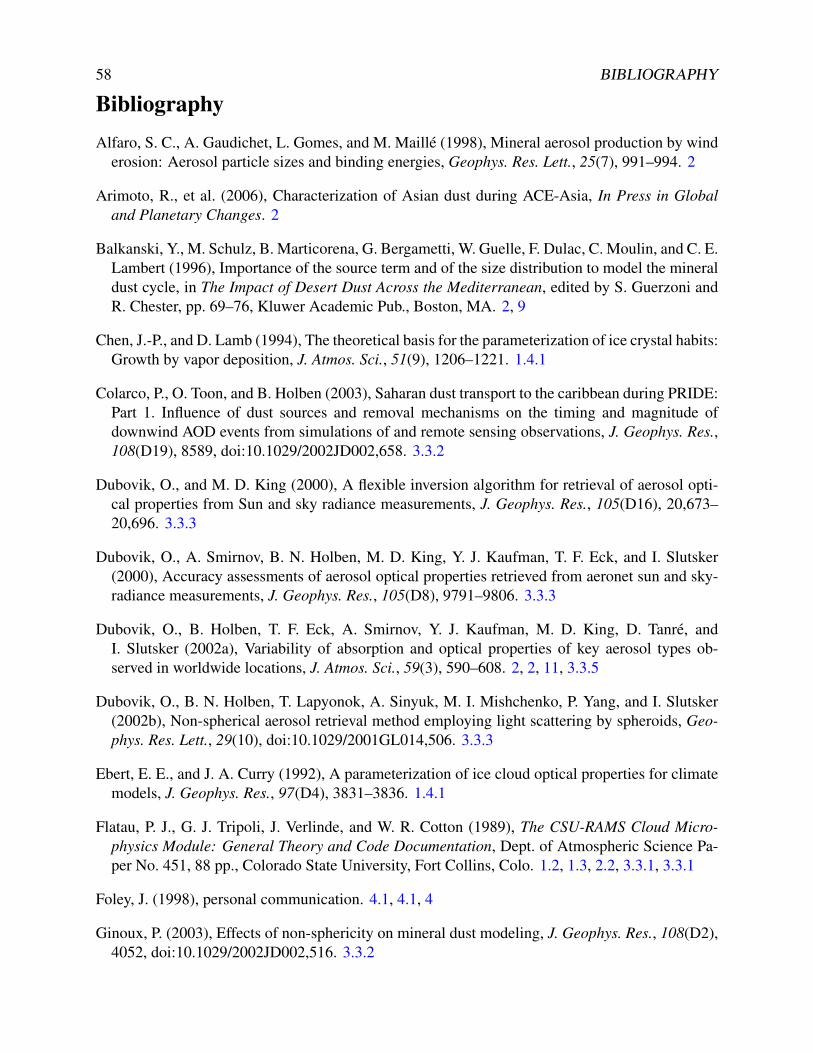
58 BIBLIOGRAPHY
BibliographyAlfaro, S. C., A. Gaudichet, L. Gomes, and M. Maille (1998), Mineral aerosol production by wind
erosion: Aerosol particle sizes and binding energies, Geophys. Res. Lett., 25(7), 991–994. 2
Arimoto, R., et al. (2006), Characterization of Asian dust during ACE-Asia, In Press in Globaland Planetary Changes. 2
Balkanski, Y., M. Schulz, B. Marticorena, G. Bergametti, W. Guelle, F. Dulac, C. Moulin, and C. E.Lambert (1996), Importance of the source term and of the size distribution to model the mineraldust cycle, in The Impact of Desert Dust Across the Mediterranean, edited by S. Guerzoni andR. Chester, pp. 69–76, Kluwer Academic Pub., Boston, MA. 2, 9
Chen, J.-P., and D. Lamb (1994), The theoretical basis for the parameterization of ice crystal habits:Growth by vapor deposition, J. Atmos. Sci., 51(9), 1206–1221. 1.4.1
Colarco, P., O. Toon, and B. Holben (2003), Saharan dust transport to the caribbean during PRIDE:Part 1. Influence of dust sources and removal mechanisms on the timing and magnitude ofdownwind AOD events from simulations of and remote sensing observations, J. Geophys. Res.,108(D19), 8589, doi:10.1029/2002JD002,658. 3.3.2
Dubovik, O., and M. D. King (2000), A flexible inversion algorithm for retrieval of aerosol opti-cal properties from Sun and sky radiance measurements, J. Geophys. Res., 105(D16), 20,673–20,696. 3.3.3
Dubovik, O., A. Smirnov, B. N. Holben, M. D. King, Y. J. Kaufman, T. F. Eck, and I. Slutsker(2000), Accuracy assessments of aerosol optical properties retrieved from aeronet sun and sky-radiance measurements, J. Geophys. Res., 105(D8), 9791–9806. 3.3.3
Dubovik, O., B. Holben, T. F. Eck, A. Smirnov, Y. J. Kaufman, M. D. King, D. Tanre, andI. Slutsker (2002a), Variability of absorption and optical properties of key aerosol types ob-served in worldwide locations, J. Atmos. Sci., 59(3), 590–608. 2, 2, 11, 3.3.5
Dubovik, O., B. N. Holben, T. Lapyonok, A. Sinyuk, M. I. Mishchenko, P. Yang, and I. Slutsker(2002b), Non-spherical aerosol retrieval method employing light scattering by spheroids, Geo-phys. Res. Lett., 29(10), doi:10.1029/2001GL014,506. 3.3.3
Ebert, E. E., and J. A. Curry (1992), A parameterization of ice cloud optical properties for climatemodels, J. Geophys. Res., 97(D4), 3831–3836. 1.4.1
Flatau, P. J., G. J. Tripoli, J. Verlinde, and W. R. Cotton (1989), The CSU-RAMS Cloud Micro-physics Module: General Theory and Code Documentation, Dept. of Atmospheric Science Pa-per No. 451, 88 pp., Colorado State University, Fort Collins, Colo. 1.2, 1.3, 2.2, 3.3.1, 3.3.1
Foley, J. (1998), personal communication. 4.1, 4.1, 4
Ginoux, P. (2003), Effects of non-sphericity on mineral dust modeling, J. Geophys. Res., 108(D2),4052, doi:10.1029/2002JD002,516. 3.3.2
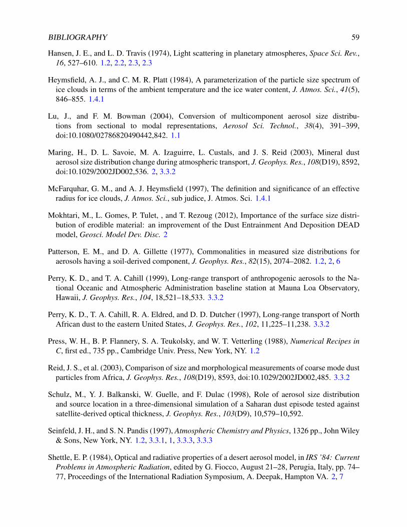
BIBLIOGRAPHY 59
Hansen, J. E., and L. D. Travis (1974), Light scattering in planetary atmospheres, Space Sci. Rev.,16, 527–610. 1.2, 2.2, 2.3, 2.3
Heymsfield, A. J., and C. M. R. Platt (1984), A parameterization of the particle size spectrum ofice clouds in terms of the ambient temperature and the ice water content, J. Atmos. Sci., 41(5),846–855. 1.4.1
Lu, J., and F. M. Bowman (2004), Conversion of multicomponent aerosol size distribu-tions from sectional to modal representations, Aerosol Sci. Technol., 38(4), 391–399,doi:10.1080/02786820490442,842. 1.1
Maring, H., D. L. Savoie, M. A. Izaguirre, L. Custals, and J. S. Reid (2003), Mineral dustaerosol size distribution change during atmospheric transport, J. Geophys. Res., 108(D19), 8592,doi:10.1029/2002JD002,536. 2, 3.3.2
McFarquhar, G. M., and A. J. Heymsfield (1997), The definition and significance of an effectiveradius for ice clouds, J. Atmos. Sci., sub judice, J. Atmos. Sci. 1.4.1
Mokhtari, M., L. Gomes, P. Tulet, , and T. Rezoug (2012), Importance of the surface size distri-bution of erodible material: an improvement of the Dust Entrainment And Deposition DEADmodel, Geosci. Model Dev. Disc. 2
Patterson, E. M., and D. A. Gillette (1977), Commonalities in measured size distributions foraerosols having a soil-derived component, J. Geophys. Res., 82(15), 2074–2082. 1.2, 2, 6
Perry, K. D., and T. A. Cahill (1999), Long-range transport of anthropogenic aerosols to the Na-tional Oceanic and Atmospheric Administration baseline station at Mauna Loa Observatory,Hawaii, J. Geophys. Res., 104, 18,521–18,533. 3.3.2
Perry, K. D., T. A. Cahill, R. A. Eldred, and D. D. Dutcher (1997), Long-range transport of NorthAfrican dust to the eastern United States, J. Geophys. Res., 102, 11,225–11,238. 3.3.2
Press, W. H., B. P. Flannery, S. A. Teukolsky, and W. T. Vetterling (1988), Numerical Recipes inC, first ed., 735 pp., Cambridge Univ. Press, New York, NY. 1.2
Reid, J. S., et al. (2003), Comparison of size and morphological measurements of coarse mode dustparticles from Africa, J. Geophys. Res., 108(D19), 8593, doi:10.1029/2002JD002,485. 3.3.2
Schulz, M., Y. J. Balkanski, W. Guelle, and F. Dulac (1998), Role of aerosol size distributionand source location in a three-dimensional simulation of a Saharan dust episode tested againstsatellite-derived optical thickness, J. Geophys. Res., 103(D9), 10,579–10,592.
Seinfeld, J. H., and S. N. Pandis (1997), Atmospheric Chemistry and Physics, 1326 pp., John Wiley& Sons, New York, NY. 1.2, 3.3.1, 1, 3.3.3, 3.3.3
Shettle, E. P. (1984), Optical and radiative properties of a desert aerosol model, in IRS ’84: CurrentProblems in Atmospheric Radiation, edited by G. Fiocco, August 21–28, Perugia, Italy, pp. 74–77, Proceedings of the International Radiation Symposium, A. Deepak, Hampton VA. 2, 7
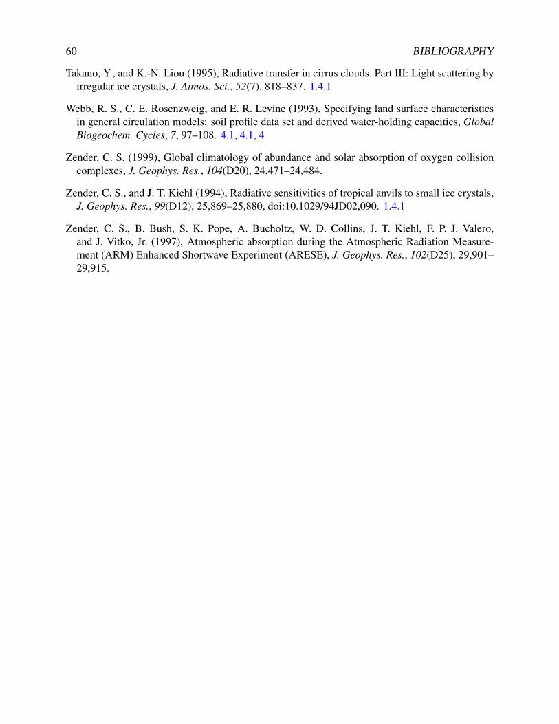
60 BIBLIOGRAPHY
Takano, Y., and K.-N. Liou (1995), Radiative transfer in cirrus clouds. Part III: Light scattering byirregular ice crystals, J. Atmos. Sci., 52(7), 818–837. 1.4.1
Webb, R. S., C. E. Rosenzweig, and E. R. Levine (1993), Specifying land surface characteristicsin general circulation models: soil profile data set and derived water-holding capacities, GlobalBiogeochem. Cycles, 7, 97–108. 4.1, 4.1, 4
Zender, C. S. (1999), Global climatology of abundance and solar absorption of oxygen collisioncomplexes, J. Geophys. Res., 104(D20), 24,471–24,484.
Zender, C. S., and J. T. Kiehl (1994), Radiative sensitivities of tropical anvils to small ice crystals,J. Geophys. Res., 99(D12), 25,869–25,880, doi:10.1029/94JD02,090. 1.4.1
Zender, C. S., B. Bush, S. K. Pope, A. Bucholtz, W. D. Collins, J. T. Kiehl, F. P. J. Valero,and J. Vitko, Jr. (1997), Atmospheric absorption during the Atmospheric Radiation Measure-ment (ARM) Enhanced Shortwave Experiment (ARESE), J. Geophys. Res., 102(D25), 29,901–29,915.
IndexCFC11 vmr clm, 45CFC12 vmr clm, 45CH4 vmr clm, 45CO2 vmr clm, 45N2O vmr clm, 45RH ice, 45RH lqd, 29, 45RH, 45abc flg, 29abs bb SAS, 37abs bb atm, 37abs bb sfc, 37abs ncl wk mdm flg, 29abs nst SAS, 37abs nst atm, 37abs nst sfc, 37abs spc SAS, 37abs spc atm, 37abs spc sfc, 37alb sfc NIR dff, 45alb sfc NIR drc, 45alb sfc vsb dff, 45alb sfc vsb drc, 45alb sfc, 37, 45alt cld btm, 37, 45alt cld mid, 45alt cld thick, 37, 45alt cld top, 45alt dlt, 45alt ntf, 37, 45alt, 37, 45asp rat hxg dfl, 29asp rat lps dfl, 30azi dgr, 37azi, 37bch flg, 29bnd SW LW, 30bnd nbr, 30bnd, 37cld frc, 45cmp aer, 26cmp cor, 30cmp mdm, 30
cmp mnt, 30cmp mtx, 30cmp ncl, 30cmp prt, 30cnc CFC11, 46cnc CFC12, 46cnc CH4, 45cnc CO2, 45cnc H2OH2O, 46cnc H2O, 46cnc N2O, 46cnc N2, 46cnc NO2, 46cnc O2O2, 46cnc O2 cnc N2, 46cnc O2 cnc O2, 46cnc O2 npl N2 clm, 46cnc O2 npl N2, 46cnc O2 npl O2 clm frc, 46cnc O2 npl O2 clm, 46cnc O2 npl O2, 46cnc O2, 46cnc O3, 46cnc OH, 46cnc dry air, 46cnc mst air, 46cnc nbr anl dfl, 30cnc nbr pcp anl, 30coat flg, 29cpv foo, 30dbg lvl, 30dmn frc, 30dmn nbr max, 30dmn rcd, 30dmt dtc, 30dmt nma mcr, 30dmt pcp nma mcr, 30dmt swa mcr, 30dmt vma mcr, 30dns CFC11, 47dns CFC12, 47dns CH4, 47dns CO2, 46
61
62 INDEX
dns H2OH2O, 47dns H2O, 47dns N2O, 47dns N2, 47dns NO2, 47dns O2O2, 47dns O2 dns N2, 47dns O2 dns O2, 47dns O2 mpl N2 clm, 47dns O2 mpl N2, 47dns O2 mpl O2 clm, 47dns O2 mpl O2, 47dns O2, 47dns O3, 47dns OH, 47dns aer, 47dns bga, 47dns cor, 30dns dry air, 47dns mdm, 31dns mnt, 31dns mst air, 47dns mtx, 31dns ncl, 31dns prt, 31doy, 31drc dat, 31drc in, 31drc out, 31drv rds nma flg, 29dsd dbg mcr, 31dsd mnm mcr, 31dsd mxm mcr, 31dsd nbr, 31eqn time sec, 48ext cff mss aer, 48ext cff mss bga, 48fdg flg, 29fdg idx, 31fdg val, 31fl err, 31fl idx rfr cor, 31fl idx rfr mdm, 31fl idx rfr mnt, 31fl idx rfr mtx, 31
fl idx rfr ncl, 31fl idx rfr prt, 31fl slr spc, 31flt foo, 31flx LW dwn sfc, 32flx SW net gnd, 32flx SW net vgt, 32flx abs atm rdr, 37flx bb abs atm, 37flx bb abs sfc, 37flx bb abs ttl, 38flx bb abs, 38flx bb dwn TOA, 38flx bb dwn dff, 38flx bb dwn drc, 38flx bb dwn sfc, 38flx bb dwn, 38flx bb net, 38flx bb up, 38flx frc drc sfc cmd ln, 32flx nst abs atm, 38flx nst abs sfc, 38flx nst abs ttl, 38flx nst abs, 38flx nst dwn TOA, 38flx nst dwn sfc, 38flx nst dwn, 38flx nst net, 38flx nst up, 38flx slr frc, 38flx spc abs SAS, 38flx spc abs atm, 39flx spc abs sfc, 39flx spc abs, 39flx spc act pht TOA, 39flx spc act pht sfc, 39flx spc dwn TOA, 39flx spc dwn dff, 39flx spc dwn drc, 39flx spc dwn sfc, 39flx spc dwn, 39flx spc pht dwn sfc, 39flx spc up, 39flx vlm pcp rsl, 32frc ice ttl, 39, 48
INDEX 63
frc ice, 48frc str zen ngl sfc, 48ftn fxd flg, 29gas cst mst air, 48gmt day, 48gmt doy, 48gmt hr, 48gmt mnt, 48gmt mth, 48gmt sec, 48gmt ydy, 48gmt yr, 48grv, 48gsd anl dfl, 32gsd pcp anl, 32hgt mdp, 32hgt rfr, 32hgt zpd dps cmd ln, 32hgt zpd mbl, 32hrz flg, 29htg rate bb, 39htg, 35hxg flg, 29idx rfr cor usr, 32idx rfr mdm usr, 32idx rfr mnt usr, 32idx rfr mtx usr, 32idx rfr ncl usr, 32idx rfr prt usr, 32j NO2, 39j spc NO2 sfc, 39lat cos, 48lat dgr, 32, 39, 48lat, 48lbl sng, 32lbl, 35lcl time hr, 39, 48lcl yr day, 39, 48levp, 39, 49lev, 39, 48lgn nbr, 32lmt day, 49lmt doy, 49lmt hr, 49lmt mnt, 49
lmt mth, 49lmt sec, 49lmt ydy, 49lmt yr, 49lnd frc dry, 32lon dgr, 49lon sec, 49lon, 49ltst day, 49ltst doy, 49ltst hr, 49ltst mnt, 49ltst mth, 49ltst sec, 49ltst ydy, 49ltst yr, 49mca flg, 29mie flg, 29mie, 5, 26, 28mmw mst air, 49mmw prt, 32mno lng dps cmd ln, 33mpc CFC11, 50mpc CFC12, 50mpc CH4, 49mpc CO2, 49mpc CWP, 39, 50mpc H2OH2O, 50mpc H2O, 50mpc IWP, 50mpc LWP, 50mpc N2O, 49mpc N2, 50mpc NO2, 50mpc O2O2, 50mpc O2, 50mpc O3 DU, 50mpc O3, 50mpc OH, 50mpc aer, 50mpc bga, 50mpc dry air, 50mpc mst air, 50mpl CFC11, 50mpl CFC12, 50
64 INDEX
mpl CH4, 50mpl CO2, 50mpl CWP, 50mpl H2OH2O, 51mpl H2O, 51mpl IWP, 51mpl LWP, 51mpl N2O, 50mpl N2, 51mpl NO2, 51mpl O2O2, 51mpl O2, 51mpl O3, 51mpl OH, 51mpl aer, 51mpl bga, 51mpl dry air, 51mpl mst air, 51mss frc cly, 33mss frc snd, 33ncks, 29nc, 35ngl nbr, 33no abc flg, 29no bch flg, 29no hrz flg, 29no mie flg, 29no wrn ntp flg, 29npc CFC11, 51npc CFC12, 51npc CH4, 51npc CO2, 51npc H2OH2O, 51npc H2O, 51npc N2O, 51npc N2, 51npc NO2, 51npc O2O2, 51npc O2, 52npc O3, 52npc OH, 52npc dry air, 52npc mst air, 52npl CFC11, 52npl CFC12, 52
npl CH4, 52npl CO2, 52npl H2OH2O, 52npl H2O, 52npl N2O, 52npl N2, 52npl NO2, 52npl O2O2, 52npl O2, 52npl O3, 52npl OH, 52npl dry air, 52npl mst air, 52nrg pht, 40nsz, 35ntn bb aa, 40ntn bb mean, 40ntn spc aa ndr sfc, 40ntn spc aa ndr, 40ntn spc aa sfc, 40ntn spc aa zen sfc, 40ntn spc aa zen, 40ntn spc chn, 40ntn spc mean, 40odac spc aer, 40odac spc bga, 40odac spc ice, 40odac spc lqd, 40odal obs aer, 40odal obs bga, 40odsl obs aer, 40odsl obs bga, 40odxc obs aer, 40, 52odxc obs bga, 40, 52odxc spc CO2, 40odxc spc H2OH2O, 40odxc spc H2O, 41odxc spc NO2, 41odxc spc O2N2, 41odxc spc O2O2, 41odxc spc O2, 41odxc spc O3, 41odxc spc OH, 41odxc spc Ray, 41odxc spc aer, 41
INDEX 65
odxc spc bga, 41odxc spc ice, 41odxc spc lqd, 41odxc spc ttl, 41odxl obs aer, 41, 52odxl obs bga, 41, 53oneD foo, 53oro, 33, 48plr cos, 41plr dgr, 41plr, 41pnt typ idx, 33ppr CFC11, 53ppr CFC12, 53ppr CH4, 53ppr CO2, 53ppr H2OH2O, 53ppr H2O, 53ppr N2O, 53ppr N2, 53ppr NO2, 53ppr O2O2, 53ppr O2, 53ppr O3, 53ppr OH, 53ppr dry air, 53prs cld btm, 53prs cld mid, 53prs cld thick, 53prs cld top, 53prs dlt, 53prs mdp, 33prs ntf, 33, 53prs sfc, 54prs, 53psd.pl, 27psd ntg dgn, 35psd typ, 26, 33q CFC11, 54q CFC12, 54q CH4, 54q CO2, 54q H2OH2O rcp q H2O, 54q H2OH2O, 54q H2O vpr, 33
q H2O, 54q N2O, 54q N2, 54q NO2, 54q O2O2, 54q O2, 54q O3, 54q OH, 54qst H2O ice, 54qst H2O lqd, 54r CFC11, 54r CFC12, 54r CH4, 54r CO2, 54r H2OH2O, 54r H2O, 54r N2O, 54r N2, 55r NO2, 55r O2O2, 55r O2, 55r O3, 55r OH, 55rds fct ice, 55rds fct lqd, 55rds ffc gmm mcr, 33rds nma mcr, 33rds swa mcr, 33rds vma mcr, 33rfl bb SAS, 41rfl bb sfc, 41rfl gnd dff, 33rfl nst SAS, 41rfl nst sfc, 41rfl spc SAS, 42rgh len, 55rgh mmn dps cmd ln, 33rgh mmn ice std, 33rgh mmn mbl, 33rgh mmn smt, 33scl hgt, 55sfc ems, 55sfc typ, 33slf tst typ, 33slr azi dgr, 55
66 INDEX
slr crd gmm dgr, 55slr cst, 33, 55slr dcl dgr, 55slr dmt dgr, 55slr dst au, 55slr elv dgr, 55slr flx TOA, 55slr flx nrm TOA, 55slr hr ngl dgr, 55slr rfr ngl dgr, 55slr rgt asc dgr, 55slr spc key, 33slr zen ngl cos, 34, 42, 55slr zen ngl dgr, 56slr zen ngl, 56slv sng, 34snow depth, 56snw hgt lqd, 34soi typ, 34spc abb sng, 34spc heat mst air, 56spc heat prt, 34spc idx sng, 34ss alb cmd ln, 34sz dbg mcr, 34sz grd sng, 34sz grd, 26sz mnm mcr, 34sz mnm, 26sz mxm mcr, 34sz mxm, 26sz nbr, 26, 34sz prm rsn, 34tau prs, 42tau, 42thr nbr, 34time lmt, 56time ltst, 56time unix, 56tm dlt, 34tpt bbd wgt, 34tpt cls ntf, 56tpt cls, 56tpt gnd, 34tpt ice, 34
tpt mdp, 34tpt ntf, 42, 56tpt prt, 34tpt sfc, 56tpt skn, 56tpt soi, 34tpt sst, 34tpt vgt, 34tpt vrt, 56tpt, 42, 56trn bb atm, 42trn nst atm, 42trn spc atm CO2, 42trn spc atm H2OH2O, 42trn spc atm H2O, 42trn spc atm NO2, 42trn spc atm O2N2, 42trn spc atm O2O2, 42trn spc atm O2, 42trn spc atm O3, 42trn spc atm OH, 42trn spc atm Ray, 42trn spc atm aer, 42trn spc atm bga, 42trn spc atm ice, 42trn spc atm lqd, 42trn spc atm ttl, 43tst sng, 35var ffc gmm, 35vlm frc mntl, 35vmr CFC11, 56vmr CFC12, 56vmr CH4, 56vmr CO2, 35, 56vmr H2OH2O, 56vmr H2O, 56vmr HNO3 gas, 35vmr N2O, 56vmr N2, 56vmr NO2, 56vmr O2O2, 56vmr O2, 57vmr O3, 57vmr OH, 57vts flg, 29
INDEX 67
vwc sfc, 35wbl shp, 35wnd frc dps cmd ln, 35wnd mrd mdp, 35wnd znl mdp, 35wrn ntp flg, 29wvl ctr, 43wvl dbg mcr, 35wvl dlt mcr, 35wvl dlt, 43wvl grd sng, 35wvl grd, 43wvl max, 43wvl mdp mcr, 35wvl min, 43wvl mnm mcr, 35wvl mxm mcr, 35wvl nbr, 35wvl obs aer, 43, 57wvl obs bga, 43, 57wvn ctr, 43wvn dlt xcm, 35wvn dlt, 43wvn max, 43wvn mdp xcm, 35wvn min, 43wvn mnm xcm, 35wvn mxm xcm, 35wvn nbr, 35xnt fac, 57xpt dsc, 35
AERONET, 14almucantar, 14arithmetic mean size, 4aspherical particles, 3average size, 4
bounded distribution, 16
columnar volume, 16command line arguments, 28convention, 4cumulative concentration, 2, 7, 16
differential number concentration, 4
distribution function, 2dust emissions, 18
effective diameter, 22effective radius, 22effective size, 5effective variance, 5equivalent area spherical radius, 3equivalent diameter, 3equivalent radius, 3equivalent volume spherical radius, 3error function, 6, 16, 17, 27
fields, 36, 44
gamma distribution, 5geometric optics, 22geometric standard deviation, 6, 16gravitational sedimentation, 22
independent variable, 3input switches, 26
Legendre expansion, 32lognormal distribution, 6lognormal distribution function, 6lower bound concentration, 2
mass distribution, 19mdlsxn, 2mean size, 4mean value, 4median diameter, 19, 20median radius, 2Mie theory, 3mineral dust, 3, 18modal diameter, 19mode, 19mode diameter, 19, 19moment, 21monodisperse distribution, 22multimodal distribution, 20multimodal istributions, 20
nomenclature, 2normal distribution, 5normalization constant, 23
68 INDEX
number concentration, 22number distribution, 19number mean size, 4number-weighted mean size, 4
overlap factors, 18overlapping distributions, 18
PDF, 3Perl, 27PRIDE, 13probability density functions, 3
radiative transfer, 3
scattering cross-section, 22SI, 15sink bins, 18size distribution, 2source bins, 18source distributions, 18spectral density function, 2spherical particles, 4standard deviation, 5surface-weighted diameter, 22
truncated concentration, 2
variance, 5, 16volume-weighted diameter, 22
![[Chapter 5. Multivariate Probability Distributions]people.math.umass.edu/~daeyoung/Stat515/Chapter5.pdf · [Chapter 5. Multivariate Probability Distributions] ... ity distributions](https://img.pdfslide.us/doc/110x75/5b32d34e7f8b9a2c328dc4ef/chapter-5-multivariate-probability-distributions-daeyoungstat515chapter5pdf.jpg)