Embed Size (px)
Citation preview

Alldredge and Gotschalk, 1988 (panel “b” scale bar = 1 cm, others = 1 mm)
gel. Prior to freezing, the position of the aggregate was
marked to facilitate the localization of the sample when
mounted on the cryotome.Aggregates embedded in situ in the drifting traps were cut
out directly from the frozen collection cup using a small
corer. The frozen embedded samples were mounted on a
CM-3050S cryostat (Leica Biosystems). Knowing the position
of the embedded aggregate, the block containing the sample
was cut to size with a razor blade for better handling. Using
an object temperature of 2308C and a chamber temperature
of 2358C, samples were cut into sections ranging from 5 lm
to 100 lm (Fig. 2e). Immediately after cutting, sections were
mounted on SuperfrostTM Plus slides (ThermoFisher Scien-
tific) and stored at 48C for short-term processing (within
weeks) or at 2208C for longer-term storage (months to
years). For microscopic examination, sections were embed-
ded in mounting medium made up of 80% (v/v) Citifluor
AF1 (Electron Microscopy Sciences) and 20% (v/v) Vecta-
shield (Vector Laboratories) and covered with a cover slip
(ThermoFisher Scientific). The cover slip was sealed with nail
polish to avoid smearing the underlying sample.
Visualization and imaging of the aggregate matrixStaining of EPSTo visualize the EPS matrix, we stained aggregate sections
with dyes commonly used for marine snow such as Alcian Blue
and Coomassie Brilliant Blue and tested dyes targeting differ-
ent EPS fractions, including Ruthenium Red, Periodic Acid
Schiff-base stain, and the fluorophore-conjugated lectin stain
Concanavalin A. Acidic polysaccharides were stained with 0.2lm-filtered 0.02% Alcian Blue (Sigma-Aldrich) dissolved in0.06% (v/v) acetic acid (pH 2.5) for 5 s and washed with ultra-pure water (UPW; Passow and Alldredge 1995; Long and Azam
1996). A-mannopyranosyl- and a-glucopyranosyl residues ofother EPS fractions were targeted with Concanavalin A conju-gated with FITC (FITC-ConA; Sigma-Aldrich) or Alexa647(Alexa647-ConA; Life Technologies) dissolved in 0.3% NaClwas tested at concentrations ranging from 100 lg/mL to 1000
lg/mL (after Uthicke et al. 2009). Proteinaceous particles werestained with Coomassie Brilliant Blue (Sigma-Aldrich). Proteinswere stained with 0.2 lm-filtered 0.04% (w/v) Coomassie Bril-liant Blue G-250 dissolved in UPW (pH 7.4) for 30 s and washed
with UPW (Passow and Alldredge 1995; Long and Azam 1996).Glycosaminoglycans were stained with 0.05% (w/v) Ruthe-nium Red (Sigma-Aldrich) dissolved in UPW for 10 min fol-lowed by washing with UPW (Tiessen and Stewart 1988), andwith a Periodic Acid-Schiff kit (Sigma-Aldrich) following the
protocol enclosed. Briefly, sections were stained with PeriodicAcid Solution for 5 min, with Schiff’s reagent for 15 min andcounterstained with Hematoxylin Solution, Gill No. 3, for 90 sincluding intermediate washing steps with UPW.
All stains were applied to untreated sections as well as tosections embedded in 25 lL 0.1% LE agarose prior to stain-ing to test if agarose-embedding can minimize sample loss,as reported for filtered samples. (N.B. in this study, “agarose-
embedding” refers to applying a drop of agarose to the sam-ple, and must not to be confused with embedding of intactwhole aggregates in agarose).
Fig. 2. Collecting and embedding marine snow in situ (counter-clockwise). (a) annotated sediment trap cylinder (SW 5 seawater; NaCl 5 sodiumchloride); (b) top view of gel collection cup with in situ embedded aggregates; (c) close-up of the gel cup; (d) microscopic image of gel-embeddedaggregate; (e) 10 lm thin-section of in situ embedded aggregate.
Flintrop et al. Embedding and slicing of marine snow
342
Flintrop et al. 2018
Particle imagingMeg Estapa, Ocean Optics Course 2021

Why particle imaging?(i.e., What information content do you gain? What processes are captured?)
Emphasis today on
• Particles ~100 um and larger (mostly)• In situ techniques (mostly)• Digital systems
*not* remote sensing images! (those will come later...)

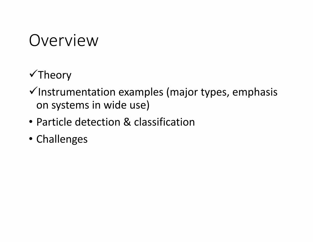
Overview
• Theory • Instrumentation examples (major types, emphasis
on systems in wide use)• Particle detection & classification

Lombard et al. Quantitative Observations of Plankton Ecosystem
FIGURE 1 | Comparison of the total size range of plankton (in equivalent spherical diameter; ESD) that available optical and imaging methods can sample. Dashed
lines represent the total operational size range from commercial information while the red line represent the practical size range which is efficient to obtain quantitative
information, for an example see Figure 2. Drawings by Justine Courboules.
3.4.2.2. Laboratory and in situ imaging systemsIn order to obtain quantitative information on plankton >
100 µm, larger volumes of water need to be examined than ispossible with IFCs. In situ imaging is non-destructive and canbe combined with net sampling. However, there are numerouschallenges. The most important criterion is the optimization ofthe trade-off between sensitivity, resolution, contrast and depthof field so that image quality allows taxonomic identificationwhile the imaged volume is large enough for statistically relevantestimations of concentrations.
High magnification imaging at short distances results in adepth of field (DOF) of only a few millimeters and thus, in a highproportion of out-of-focus images not limited to the DOF (e.g.,Schulz, 2013). To avoid motion blurring, short shutter speeds ofa few microseconds are required (e.g., Davis et al., 1992; Schulz,2013). Illumination adapted to the in situ and towing conditionsshould guarantee the image quality and high signal-to-noise ratioof the camera. Imaging systems can be adapted to illuminate acalibrated volume of water for more precise quantification ofplankton and particles (Picheral et al., 2010). Due to the above-described trade-offs, in situ systems have a relatively restrictedsize range of operation and focus either on small size classes witha small volume imaged (e.g., CPICS, LOKI), where imaging ofsizes less than a few millimeters with a high depth of field isclose to the feasible border of the physical laws of optics (Schulz,
2013), or target larger fields of views with less details on organismmorphology.
Another method to overcome the in situ constrains is touse imaging methods on net-collected plankton samples. In thiscase the conditions required for an optimal field of view andDOF may be met. However, net tows integrate the planktonover towing distances and can be intrusive, damaging someof the collected organisms. Plankton samples from nets maybe imaged either by flow-through chambers (e.g., FlowCam-Macro, LOKI) or plankton scanners such as the ZooScan (Gorskyet al., 2010). Flow-through techniques limit the maximal size oforganisms observable to the minimal diameter of its tubing. Toavoid clogging, larger individuals are removed prior to analysis.Scanner-based approaches cannot be used in situ and are difficultto use at sea. Samples therefore have to be treated with fixativesthat can modify the chemical composition of organisms, theircolor and, in some cases, their morphology. in situ imagingprovides an alternative to study fragile taxa, such as gelatinousorganisms, which may be damaged or destroyed by net tows(Remsen et al., 2004; Stemmann et al., 2008a).
In the following section, a selection of plankton imagingdevices (other than the IFCs discussed above) that arecommercially available, along with their imaging approach, arebriefly introduced (more details are available in Table 1). As ageneral rule, information content on plankton increases with
Frontiers in Marine Science | www.frontiersin.org 9 April 2019 | Volume 6 | Article 196
Particle size ranges, optical modeling regimes, and particle sizing/imaging instruments
Upper: Clavano et al. 2007; lower: Lombard et al. 2019
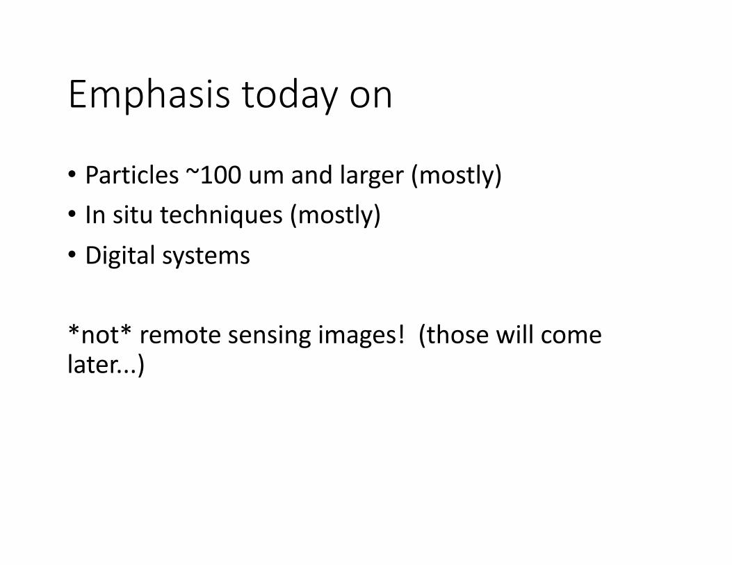
Optical resolution of an imaging system
Figure 1.1, Ocean Optics Web Book (Mobley et al.)

Optical resolution of an imaging system
Figure 1.1, Ocean Optics Web Book (Mobley et al.)
Wikimedia Commons

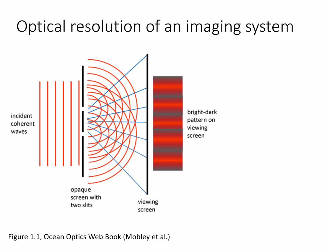
Optical resolution of an imaging system• Rayleigh criterion: Diffraction-limited horizontal resolution (r) of an imaging
system
figure: http://zeiss-campus.magnet.fsu.edu/articles/basics/resolution.html
𝑟 =1.22 𝜆𝑁𝐴 where
𝑁𝐴 = 𝑛 sin 𝛼𝑁𝐴 = 𝑛 sin(2𝛼)
if objective lens onlyif objective + condenser lenses
(NA = numerical aperture)
Optical resolution of an imaging system• Rayleigh criterion: Diffraction-limited horizontal resolution (r) of an imaging
system
• However depth of field varies in proportion to 1/(NA)2
𝑟 =1.22 𝜆𝑁𝐴 where
𝑁𝐴 = 𝑛 sin 𝛼𝑁𝐴 = 𝑛 sin(2𝛼)
if objective lens onlyif objective + condenser lenses
figure: https://www.edmundoptics.com/knowledge-center/application-notes/imaging/depth-of-field-and-depth-of-focus/

Sampling density of an imaging system• Ideally want sampling density / camera resolution (pixels per physical
length) to match optical resolution
• Nyquist sampling theorem: sampling frequency should be at least 2x the highest-frequency features in the specimen

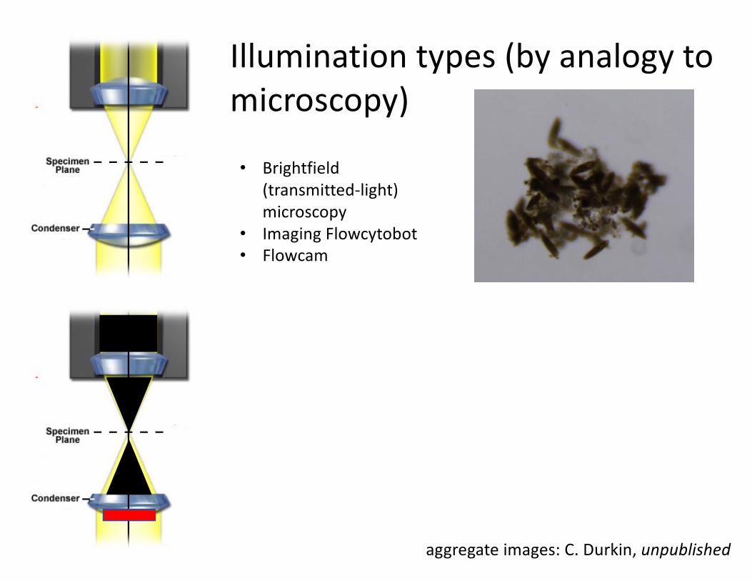
Illumination types (by analogy to microscopy)
• Brightfield (transmitted-light) microscopy
• Imaging Flowcytobot• Flowcam
aggregate images: C. Durkin, unpublished
Illumination types (by analogy to microscopy)
aggregate images: C. Durkin, unpublished
• Brightfield (transmitted-light) microscopy
• Imaging Flowcytobot• Flowcam

Illumination types (by analogy to microscopy)
aggregate images: C. Durkin, unpublished
• Brightfield (transmitted-light) microscopy
• Imaging Flowcytobot• Flowcam
• Darkfield (scattered-light) microscopy
• Underwater Vision Profiler

Illumination types (by analogy to microscopy)
Also holography, line-scanning cameras...
aggregate images: C. Durkin, unpublished
• Brightfield (transmitted-light) microscopy
• Imaging Flowcytobot• Flowcam
• Darkfield (scattered-light) microscopy
• Underwater Vision Profiler

Overview
üTheory • Instrumentation examples (major types, emphasis
on systems in wide use)• Particle detection & classification• Challenges

Fluidics system—Imaging FlowCytobot’s fluidics system (Fig. 2) is based on that of a conventional flow cytometer: hydro-dynamic focusing of a seawater sample stream in a particle-freesheath flow carries cells in single file through a laser beam(and then through the camera’s field of view). The fluidics andsampling system is similar to that of the original FlowCytobotexcept that, to minimize problems due to settling of large par-ticles, the syringe is mounted vertically rather than horizon-tally and the flow through the flow cell is downward ratherthan upward.
The sheath fluid, seawater forced through a pair of 0.2- m mfilter cartridges (Supor; Pall Corp.) by a gear pump (Micropump,Inc. Model 188 with PEEK gears), flows through a conical cham-ber to a quartz flow cell. The flow cell housing and sample injec-tion tube is from a Becton Dickinson FACScan flow cytometer,but the flow cell is replaced by a custom cell with a wider chan-nel (channel dimensions 860 by 180 m m; Hellma Cells, Inc.).Because the FACScan objective lens housing, which normallysupports the plastic flow cell assembly, is not used here, an alu-minum plate (3.175 mm thick) is bolted to the assembly.
A programmable syringe pump (Versapump 6 with 48,000-step resolution, using a 5-mL syringe with Special-K plunger;Kloehn, Inc.) is used to sample seawater through a 130-m m
Nitex screen (to prevent flow cell clogging), which is protectedagainst biofouling by 1 mm copper mesh. The sample water isthen injected through a stainless steel tube (1.651 mm OD,0.8382 mm internal diameter; Small Parts, Inc.) into the cen-ter of the sheath flow in the cone above the flow cell. The tub-ing is of PEEK material (3.175 by 1.575 mm external and inter-nal diameter for sheath tubes, 1.588 by 0.762 mm for others;Upchurch Scientific).
An 8-port ceramic distribution valve (Kloehn, Inc.) allowsthe syringe pump to carry out several functions in additionto seawater sampling. These include regular (~daily) additionof sodium azide to the sheath fluid (final concentration~0.01%) to prevent biofouling, and regular (~daily) analysesof beads (20 or 9 m m red-fluorescing beads; Duke Scientific,Inc.) as internal standards to monitor instrument perform-ance. In addition, during bead analyses (~20 min d–1), thesample tubing (which is not protected from biofouling bycontact with azide-containing sheath fluid) is treated withdetergent (5% Contrad/1% Tergazyme mixture) to removefouling. Finally, the syringe pump is used to prevent accu-mulation of air bubbles (from degassing of seawater) in theflow cell, which could disrupt the laminar flow pattern;before each sample is injected, sheath fluid is withdrawn(along with any air bubbles) through both the sample injec-tion needle and the conical region above the flow cell, anddiscarded to waste. Azide solution, suspended beads, anddetergent mixture are stored in 100-mL plastic bags withLuer fittings (Stedim Biosystems).
Olson and Sosik In situ imaging of nano- and microplankton
197
Fig. 2. Schema of fluidics system of Imaging FlowCytobot.
Fig. 3. Schema of optical layout of Imaging FlowCytobot.
9/)4"+4&:;-<02*-=-* !>;7-+&?&@-7"A%&BCCD8

G01(#="$(#*H%)%40*!#4E%'(#*I*3!%&8(#"' ($*"'>C*J-,-6
� � � � � � � � � � � � � � � � � � � � � � � � � � � � � � � � � �
� �
� 5� � 2� � � � � � � � ' � � � � � � � � � � 399= � � � � A� � . � � � � � � � � � 8 � � � � � � � � � �< � � � ! � � " # # # � � � � � � � � + � � 7 - $ � � 8 � � � � � � � � � � � " # # " � � � � � 7 - $ � � � � � � � � � � � � � � � � � � � � 8 � � � � � � � � � � � " # # " � � � � � � � � � � � � � � � � � � � � � � � � � � � � � � � � � � 1 � � � � � � � � � � � � � � � � � � � � � � � � �� � � � � � � � � � � � � � � � � � � � � � � � � � � � � � � � � � � � � � � � � � � � � � � � � � � � � � � � � � � � � � � � � � � � � � � � � � � � � � � � � � � � � � � � � � � �� � � � � � � � � � � � 2� � � . � � � � � � � � � . � � � � � � � � � � � � � � � � �� � � � � � � � � � � � � � � � � � � � � � � � � � � � � � � � � � � � � ! � � � � � � � �� � � � � � � � � � � � � � 1 � � � � � ) � � � � * � � � � � � � � � � " # # + � �
� � ? � � � � � � � � 7 � � � - � � � � � � � ? 7 - � � � � � � � � � � � � � � �� � � � � � � � � � � � � � � � � � � � � � � � � � � � E3# # � 4 � � � � � � � � � � � � � � � � ! � � �� � � � � � � � � � � � � � � � � � � � � � � � � � � � � � � � � � � � � � � � � � � � �� � � � � � � � � � � � � � � � � � � � � � � � � � � � � � � � � � � � � � � � � � � � � � � � � � �� � � � � � � � � � � � � � � � � � � . � 8 � � � � � � � � � � � � � � � � � � � � � � � �� � � � � � � � � � � � � � � � � � � " 0/ ! � � � � � � � � � � � � ? 7 - � � � � � � � � � � � � � � � � � � � � � � � � � � � � � � � � � � " � � � � � � � 0� � � � � � � � � � � � � � � � � � � � � � � � � � � � � � � � � � � � 3� � ; � � � � � � � � � � � � � � � � � . � 8 � � � � � � � � � �� � � � � � � � � � � � � < � � � � � � � � � � � 399" (� < � � � � � � � � � � � " # # # � �? 7 - " � � � � � 0� � � � � � � � � � � � � � � � � � � � � � � � � � � � � � � � � � � � � � � � � � � � � < � � � � � � � � � " # # + � � " # # 9� � � ? 7 - 0� � � � � � � � � � � � � � � � � � � � � � � � � � � � � � � � � � � � � � � � � � � � � � � � � � � � � � � � � � � � � � � � �� � � � � ! � � � � � � � � � � � ' � � � � � � � � � � � � � " # # = � � � � � � � � � � � � � � �� � � � � ? 7 - 5� � � � � � � � � � � � � � � � � � � � � � � � � � � � � � � � � � ! � � � � � � � � � � � � � � � � � � � � � � � � � � � � � � � � � � � � � � � � � � � � � � � � � � � � � � � � � � � � � � � � � � � � . � 8 � � � � � � � � � � � � � � � � � � � � � � � � � � � � � � � � � � � � � � � � � � � � � � � . � 8 � � � � � � � � � � � � � � � � � � � � � �� � � � � � � � � � � � � � � � � � � � � � � � � � C � � � � � � � � � �
/ � � � � � � � � � � � � � � ? 7 - 5� � � � � � � � � � � � � � � � � � � � � � � �� � � � � � � � � � � � � � � � � � � � � � � � � � � � � * , ? 6 � � � � � � � 6 � � � �� � � � � � � � � � � � � � � � � � � � � � � � � � � � � � � � � � � � � � ' : ' � 6 :: � � � � � � � � � � 1 � � � � � � � � � � � � � � � � � �
� � � � � � � � � � � � � � � � � � �
� � � � � � � � � � � � � � � � � � � ? 7 - � � " � � � � 0� � � � � � � � � � � � � � � � � � � �� � � � � � � � � � � � � � � 3; # # � � � � � � � � � � � � � � � � � � � � � � � � � 3993� � � � � � � � � � � � � � � � � � � � � � � � � � � � � � � � � � � � � � � � � � � � � �� � � � � � � � � � � � � � � � � � � � � � � � � � � � � � � � � � � � � � � � �� � � � � � � � 3# # # � � � � � � � � � � � � � � � � � � � � � ? 7 - 0� � � � � " 5# � � � � � � � � * � � � � � � � � � � � � � � � � � � � � � � � � � � � � � � � � � � � � � � � � �� � � � � � � � � � � � � � � � � � � � � � � � � � � � � � � � � � � � � � � � � �&� � � � � � � � � � � � � � � � � � � � � � � � � � � � � � � � � � � � � � � � � � � � � � � � � � � � � � � � � � � � � � � � � � � � � � � � � � � � � � � � � 2� � � � � � � � � � � � � � � � �� � � � � � � � � � � � � � ? 7 - � � � � � � � � � � � � � � � � � � � � � � � � � � � � � � � � � � � � � � � � � � � � � � � � � � � � � � � � � � � � � � � � � � � � � � �� � � � � � � ? 7 - 5� � � � � � � � � � � � � � � � � � � � � � � � � � � � � � � � � � � � � �. � � � � � � � � � ? 7 - 5� � � � � � � � � � � � � � � � � � � � � � � � � � � � � � � � � � � � � � �� � � � � � � � � � � � � � � � � � � � � � � � � � � � � � � � 2 � � 3� � � � � � � � � � � � � �� � � ! � � . � 8 � � � � � � � � 2 � � � 3* � � � � � ? 7 - 5� � � � � � � � � � � � � � � � � � �� � � � � � � � � � � � � � � � � � � � � � � � � � � � � � � � � � � � � � ? 7 � � � �� � � � � � � � � � � � � � � � � � � $ , 7 � � � � � � � � � � � � � � � � � � � � � � � � � � �� � � � � � � � � � �
! � � � � � � � � � � � � � � � " � � ? 7 - 5� � � � � � � � � � � � � ; # � � � �� � � � � � � � � � � � � � � � � � � � � � � � ; # # # � � � � � � � � � � � � � � � � � �� � � � � � � � � � � � � � � � � � � � � � � � � � � � � � � � � � � � � � � � � � � � � � �� � � � � � � � � � � � � � � � � � � � � � � � � � � � � � � � � � � � � � � � � � � � � � � � � � � � � � � � � � � � � � � � � � � � � � � � � � � � � � � � � � � � � � � � � � � � � � � � � � �� � � � � � � � � � � � � � � � � � � � � � � � � � � � � � � � � � � � � � � � � � �� % : 8 � � � � � � A" 5� � � � � � � � � � � � � 2 � � � 3. � �
� � � � � � � � � ' � � � � I . &� ' I 3� . . 8 � * J K � � � � � � � � � � � � � � � � � �3� ; � 6 � � � � � � � &� � � � � � � � � � � � � � � 35� / ! � � � � � � � � � � � � � � � � �= � < � � � � � � � � � � � � � � � � � � � � � � � � � � � � � � � � � � � � 3# # � � � � � � � � �� � � � � � � � � � � � � � � � � � � � � � � � � � � � � � � � � � � � � � � � � � � � � �
� � � � � , 8 2 ! � � # � � + , 6 2 ! � " � � � � � � A� � � # � % � / � � ; � ' � � � # � � � � � � � � � � � " � + , � 2 � % � � " � � � % � � � � � " � � � � � � � $ � � � � ! � � � � � � � � � # � � # � � � � � < � �� � " � � # # � " � � � � ? � # � " � � � $ � � � � , � � � ; 29 � � � � � % � � � � " � � � � � � � � � � � � � � � � � � � C� � , � � � � $ � B6 29
� � � � � � � � � � � � � � � � � � � � � � � � � � � � � � � � � �
� � .
. � � � � � � � � � � � � � � � � � � � � � � � � � � � � � � � � � � � � � � �� � � � � � � � � � � � � � � � � � � � � � � � � � � � � K � � � � � � � � � � � � � � � � �� � � � � � � � � � � � � � � � � � � � � � � � � � � � � � � � � � � � � � � � � � �� � � � � � � � � � � � � � � � � � � � � � � � � � � � � � � � � � � � � � � � � � � � � � �� � � � � � � � � � � � � � � � � � � � � � � � � � � � � � � � � � � � � � ! � �
� � � � � � � � � � � � � � � � � � � � � � � � � � � � � � � � � � � � � � � � � � �� � � � � � � � � � � � � � � � � � � � � � � � � � � � � � � � � � � � � � � � � � � � � � � � �� � � � � � � � � � � � � � � � � � � � � � � � � � � � � � � � � 335� � � 1 � � � � � � � � � � � � �� � � � � � � � � � � � � � � � � � � � � � � � �
� � � � � � � � � � � � � � � � � � � � � � � � � � � � � � � � � � � 1 � � � � � � � � � � � � ? 7 - 5� � � � � � � � � � � � � � � � � � � � � � � � � � � � � � � � " � � � � � � � � � � � � � � � � � � � � � � � � � � � � � � � � � � � � � � � 2 � � � ; * � D
� 3�
� � � ' � � � � / � � � � � � � � � � � � � � K � � � � � � � 6 � � � � � � � � � � � � �� � � � � � � � � � � 6 � � � � � � � � � � � � � � � � � � � � � � � � � � ' � � � � / � � � � ! � � � � � � � � � � � � � � � � � � � � � � � � � � � � � ! � � � � � � � � � � � � � �� � � � � � � � � � � � � � � � � � � � � � � � � � � � � � � � � � � � � � � � � � � � � � � � � � � �� � � � � � � � � � � & � � � S� � � � � D
� " �
� � � � � � � � � � � � � � � � � � � � � � � � � � � � � � � � � � � � � � � � � � �� � � � � � � � � � � � � � � � � � � � � � � � � � � � � � � � � � � � � � � � � � � � � � � ! � � � � � � � � � � � � � � � � � � � � � � � � � � � � � � � � � � � � � � � �� � � � � � � K � � � � � � � 1� � � � � � � � � � � � � � � � � � � � � � � � � � � � � � � � � � � � � � � � � � � � � � � ! � � � � � � � � � � � � � � � �� � � 3# # # � � � � � � � � � � � � � � � � � � � � � ! � � � � � � � � � � � � � � � � �� � � � � � � � � � � � � � � � � � � � � � � � � � � � � � � � � � � � � � � � � � � � � � � � � � � � � � � � � � � � � � � � � � � � � � � � � � � � � � � � � � � � � � � � � � � � � � �� � � � � � � � � ' � � � � / � � � � � � � ! � � � � � � � � � 1� � � � � � � � � �
� � � � � � � � � � � � � � � � � � � � � � � ' � G � # � # # ; � � � � � / � G � 3� ; ; 0=� 2 � � 0� � � � � � � � � 3�
# � � � � � � � ) � � � � � ) � � � � � � � 0 � � � � � � � 0 � & " � � ? 7 - 0� � � �? 7 - 5� � � � � � � � � � � � � � � � � � � � � � � � � � � � � � � � � � � � � � � � � � �� � � � � � � � � � � � � � � * , ? 6 � � � � � � � � � � 6 � � � � � � � � � ' � �8 � � � � � � � � � � � � � � � � � � � � � � � � � � � � � � � � � � � � � � � � � � � � � � � � � � � � " � � � � � � � � � � � � � � � � � � � � � � � � � � 5� � � 8 � � � � � � � "� � � � � � � � � � � ; # � � � � � � � � � � � � � � � � � � � � � � � � � � � � � � � � �� � � � � � � � � � � � � � � � � � � � � � � � � � � � � � � � � ! � � � � � � � � � � � � � � � � � � � �� � � � � � � � � � � � � � � � � � � � � � � � � � � � � � � ! � � � � � � � � � � �
S A Sm pB= .
!S S Sp i m ii
= ( )" ( )#$ %&' log log, ,
2
� � � � " � 1� � � � % � � � � � � # � % � " � � � � � � � � � � � % � � " � � � � % � � � � � � � BBE � � � � � # � ' F � % � � 9 , 82 1� � � � % � � � � � � # � % � ? � � � � � � � � � � � % � � G " A � � � � � � � � � � � #� � C � � � B� � G " 9 � � � % � � � � � � � # � � % � � � � � � � � � � � � � B� B � � � � � 9 , 6 2 1� � � � % � � � � � � # � , � $ 2 % � ? � � � � � � � � � � � % � � " " A , � � 2 � � � � � � � � # � � � � � � # � �� � � � � � � , H � � � � � � � � � � � % I 2 ' � � $ � � � � � � $ � " � � � � � � " � � � 9 � � � % � � � � � � � # � � % � � � � � � � � � � � � � " � � # � � � � � # � � � � � � � � AE � � E � � � % � � � # � �� � � ' � � � % � & 9
� � � � # � 0� � � � � # � � � � � !� � � � � � % � � � � � ? � # � � � � � % � & � � � � � � % � # % � �# � � � � � � � � � � � � % # � � � � � � � % � 9 � � � ' � � � � � � ? � # � � � $ � � � % � J � 9 � � � � � & � JB9 � � � � 9 : � � ; � � � � � � � � � � � � � � � � � � � � � � � ? � # � � � � � � !� � " " A9 � � �% � � � � � � % � � � � � � � � � � � � ? � # � � � % � # % � # � � � � � � � � � � F � % ; ; � � � � � � � �� � # < � � � 9 � � � % � � � � � � � � � � # # # � % � � � � � � � � � � � $ � � � � � � � � � � � � � � � � � � � �� " � # # � � � 9
! ^>#%-.',,%$%# ">&/,)#%,%.,>+(! C;6>$>.'")>;'&%#)L+"F;%)'(#)6>Z%")->H%)
.'">8$',>+(-)$%[F>$%#! G'$,>."%-)8%"+O)_2AA)F;)(+,)O%""U$%-+"L%#! P'$&%)5_2)P<)-';6"%)L+"F;%I>;'&%
� � � � � � � � � � � � � � � � � � � � � � � � � � � � � � � � � �
� . ;
� � � � � � � � � � � � � � � � � � � � � � � � � � � � � � � � � � � � � � � � � � � � ? 7 - 5� � � � � � � � � � � � � � � � � � � � � � � � � � � � � � � � � � � � � � � � � � � � � � � � ! � � � � � � � � � � � � � � � � � � � � � � � � � � � � � � � � � � � � � � � � � � �
� � � � � � � � � � � � � � � � � � � � � � � � � � � � � � � � � � ! � � � � � � � � �� � � � � � � � � � � � � � � � � � � � � � � � � � � � � � � � � � � � � � � � � � � � � � � � �� � � � � # � � � � 0� � � � � � � � � � � F; � 2 � � � = � � � � 9� � � � � � � � � � � � � � �� � � � � � � � � � � � � � 0� � � � � � � � � � � � � � � � � � � � � � � � � � � � � � � � � � � � �� � � � � � � � � � � 2 � � � + � � � � � � � " � � � � ; � � � � � � � � � � � � � � � � � � � � � � � � �� � � � � � � � � � � � � � � � � � � � � � � � � � � ! � � � % � � � � � � � � � � � � � � � � � � � � � � � � � � � � � � � � � � � � � � � � � � � � � � � � � � � � � � � � � � � + 5� � � � � � � � � � ; � � � � � � � � � � � F; � � � � � � � � � � � � � � � � � � � � � � � � � � � �� � � � � � � � � � � � � � � � � � 3# # � � � � $ � � � � � � � � � � � � � � � � � � � � � �� � � � � � � � 0� � � � � � � � � � � F; � � � � � + 5� 3# # � � � � � � � � � � � � � � � � � � � � � � � � � � � � � � � � � � � � & � � � � � � � � � � � � � � � � � � � � � � � � � � � � � � � � � � � � �� � � � � � � � � � � � � - � � � � � � � � � � � � � � � � � � � � � � � � � � � � � � � �� � � � � � � � � � � � � � � � � � � � � � � � � � � � � � 3� � � � � � � � � � F; �
� � � � � � � � � � ? 7 - " � � � � � � � � � � � � � � � � � � � � � � � � � � � � � � � � � C � � � �
� � � � � � 6 � � � � � � � � � ' � � � � � � � � � � � � � � � � � � � � � � � � � � � �� � � � � � � � < � � � � � � � � � � � " # # " (� ' � � � � � � � � � � � � � " # # " � � � � � ? 7 - ;� � � � � � � � � � � � � � � � � � � � � � � � � � � � � � � � � � � ? 7 - � � � � � � � � � � � � � � � � � � � � � � � � � � � � � � � � � � � � � � � � � � � � � � � � � � ? 7 - 0� � � � � �� � � � � � � � � � � � � � � � � � � � � � � � � � � � � � � � � � � � � � � � � � � � � � � � � � � � � � � � � � � � � ! � � � � � � � � � � � � � � � � � � � � � � � � � � � � � � � � � � � � � � � �� � � � � � � � � � � � � � ! � � � � � � � � � � � � � � � � � � � � � � � � � � � � � � � �� � � � � � � ' � � � � � � � � � � � � � " # # = � � � � � � � � � � � � � � � � � � � � � � � �� � � � � � � � � � � � � � � � � � � � � � � � � � � � � � � � � � � % � � � � � � �3995� � � & � � � � � � � � � � � � � � � � � � � � � � � � � � � � � � � � � � " � � � � �� � � � � ? 7 - " � � � � � ? 7 - 0� � � � � � � � � � � � � � � � � � � � � � � � � � � � � � � � � � � � � � � � � � � � � � � � � � � � � � � � � � � � � � � � � � � � � � � � � � � � � � �� � � � � � � � < � � � � � � � � � " # # + � � � 6 � � � � � � � � � � � � � � � � � � � � � � � � � � � � � � � � � � � � � � � � � � � � � � � � � � � � � � � � � � � � � � � � � � � � � � � �� � � � � � � � � � ! � � � � � � � � � � � � � � � � � � � � � � � � � � � � � � � � � � � � �� � � � � � � � � � � � ! � � � � � � � � � � � � � � � � � � � � � � � � � � � � � � � � � � � � � ! � � � � < � � � � � � � � � " # # 9� �
� � � � � � � � � � ! � � � � � � � � � � � � � � � � � � � � � � � � � � � � � � � � � � �� � � � � � � � � � � � � � � � � � � � � � � � � � � � � � � � � � � � � � � � � � � � � � � � � � � � � � � � � � � � � � � ' � � � � � � � � � � � � � " # # = � � � � ? � � � � � � � � �� � � � � � � � � � � < � � � � � � � � � � " # # = � � � � � � � � � � � � � � � � � � � ! � � � � � �� � � � � � � � � � � � � � � � � � � � � � � � � � � � � � � � � � � � � � � � � � � � � � � � � �� � � � � � � � � � � � � � � � � � � � � � � � � � � � � � � � � � � � � � � � � � � � � � �� � � � � � � � � � � � � � � � � � � � � � � � � � � � � � � � � � � � � � � � � � � � � � � � � � � � � � �� � � � � � � � � � � � � � � � � � � � � � � � � � � � � � � � � � � � � � � � � � � � � � � � � � ! � � � � � � � � � � � � � � � � � � � � � � � � � � � � � � � � � � � � � � � �� � � � � � � � � � � � � � � � � � � � � � � � � � � � � � � � � < � � � � � � � �" # # 9� � � � � ? 7 - 5� � � � � � � � � � � � � � � � � � � � � � � � � � � � � ! � � � � � �� � � � � � � � � � � � � � � � � � � � � � � � � � � � � � � � � � � � � � � � � � � � � � � �� � � � � � � � � � � � � � � � � � � � � � � � � � � � � � � � � � � � � � � � � � � � � � � � � � �� � � � � � � � � � � � � � ! � � � � � � � � � � � � � � � � � � � � � � � � � � � � � � � � < � � � � � � � � � � " # # " (� < � � � � � � � � � � � " # # ; � < � � � � � � � � � " # # + (� ' � � � � � � � �� � � � " # # = � � � � � � � � � � � � � � � � � � � � � � � � � � � � � � � � � � � � � � � � � �� � � � � � � � � � � � � � � � � � � � � � � � � � � � � � � � � � � � � � � � � � � � �� � � � � � � � � � � � � � � � � � � � � � � � � � � � � � � � � � � � � � � �
: � � � � � � � � � � � � � � � � � � � � � � � � � � � � � � � � � � � � � � � � � � � � � � � � �� � � � � � � � � � � � � � � � � � � � � � � � � � � � � � � � � � � � � � � � � � � � � % � � � � � � � � � � � 399; (� ) U� � � � " # # # � � � & � � � � � � � � � � � � � � � ! � � � � � � � � � � � � �� � � � � � � � � � � � � � � � � � � � � � � � � � � � � � � � � � � � � � � � � � � � ' � � �� � � � � � � � � � � " # # = � � �
� � � � � � � � � � � � � � � � � � � � � � � � � � � � � � � � � � � � � � � � � � � � � � � � � � � � � � � � � � � � � � � � � � � � � � � � � � � � � � � � � � � � � � � � � � � � � � � � � � � � � � � � � � � � � � � � � � � � � � � � � � � � � � � � � � � � � � � � � � � � � � � � � � �� � � � � � � � � � � � � � � � � � � � � � � � � � � � � � � � � � � � � � � � � � � � � � � � � �� � � � � � � � � � � � � � � � � � � � � � � � � � � � � � � � � � � � � � � � � � � � ' � � �� � � � � � � � � � � " # # 0� � � ' � � � � � � � � � � � � � � � � � � � � � � � � � � � � � � � � � � � � � � � � � � � � � � � � � � � � � � � � � � � � � � � � � � � � � � � � � � � � � �� � � � � � � � � � � � � � � � � � � � � � � � � � � � � � � � � � � � � � � � ) � � � � � � � � � � 399A(* � � � � � � " # # 3(� * � � � � � � � � � � � � � � " # # + � � � � � � � � � � � � � � � � � � � � � �� � � � � � � � � � � � � � � � � � � � � � � � * � � � � � � � � C � � � � � 3999(' � � � � � � � � � � � � � " # # " � �
� � � � � � � � � � � � � � * , ? 6 � � � � � � � � � 2 � � � � + F9� � � � � � �� � � � � � � � � � � � � � � � � � � � � � � � � � � � � � � � � ? 7 - � � � � � � � � � � � � � �� � � � � � � � � � � � � � � � � � � � � � � � � � � � � � � � � � � � � � � � � ! � � � � � � � � � �� � � � � � � � � 5� / ! � � � � � � � � � � � � � � � � � � � � � � � � � � � � � � � �� � � � � � � � � � 3� # " � % � � � � � � � � � � � � � � � � � � � � � � � � � � � � � � � � � � �� � � � � � � � � � � � � � � � � � � � � � � � � � � � � � � / � � � � � � � � � � � � � � � ! � � � � � � � � � � � � � � � � � � � � � � � � � � � � � � � � � � � � � � � � � � � � � � �� � � � � � � � � � � � � � � � � � � � � � � � � � � � � � � � � � � � � � � � � � � � � � � �� � � � � � � � � � � � � � � � � � � � � � � � � � � � � � � � � � / � � � � � � � � � � � � � �� � � � � � � � � � � � � � � � � � � � � � � � � � � � � � � � � � � � � � � � � � � � � � � � � � � � � � � � � � � � � � � � � � � � � � � � � � � � � � � � � * � � � �
� � � � ' � 7 � � � # � ; � � � � � % � " � � � � � " � � � 6 ) - % � � � � � � , 8 2 � � # � � + , 6 2� � � � � � � � + , � 2 % � � � � � � + , : 2 " � � � � � + , 4 2 � � � � � � � � � � + , � 2 � � � � � % � �# � � � � � + , = 2 � � � � # � � � � � + � , N 2 " � � � � � � � � � � � � � � 9 � � � ' # � % ; # � � � % � # �� � E " " 9
`/F;8('>"-)8%"+OK))-.'"%8'$-):)a);;

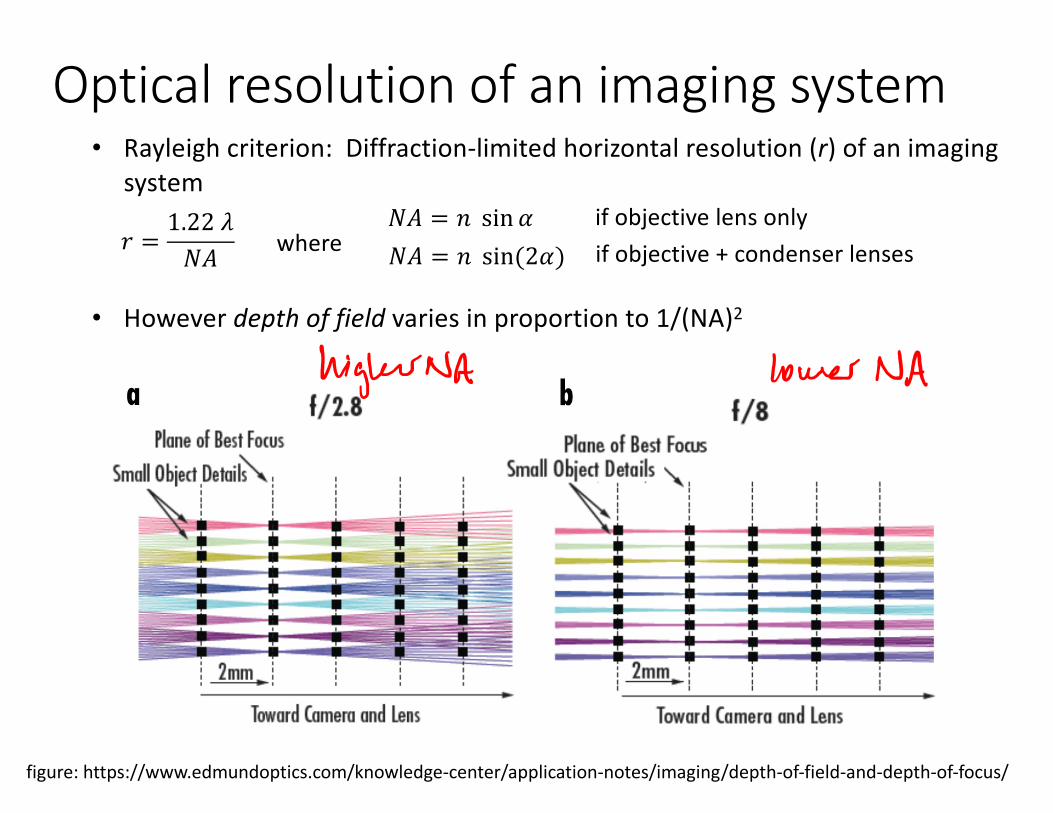
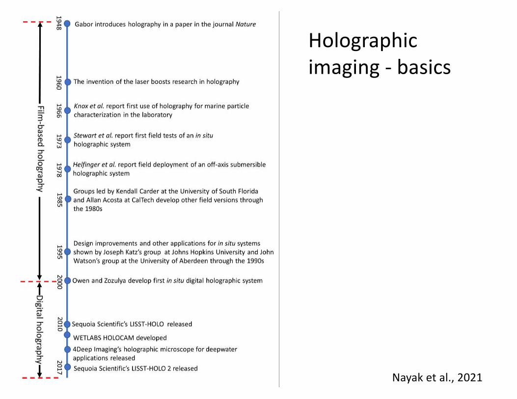
Holographic imaging - basics
• Sample volume illuminated by coherent, monochromatic light source
• Interference between diffraction pattern and the original, unscattered beam is recorded
• Computational reconstruction provides 3D image of particle size, shape, orientation
Off-axis holography
laser beams, while the developed holograms arebrought back to the reference beams to optically re-construct the 3D images of the particle fields. ACCD camera then scans the 3D image volume me-chanically, plane by plane, and the particle field in-formation is computed from the scanned images. Agood example is the holographic particle image ve-locimetry system recently developed by Pu andMeng.5,6
To resolve the spatial structures of a turbulent flowfield, millions of tracer particles are seeded in a flowdomain to a typical density of 10–30 particles!mm3.The silver-halide-based holographic plate, which of-fers a storage capacity of GBytes !several thousandline pairs per mm", is usually chosen to perform volu-metric recording of such large-volume, high-densityparticle fields. Unfortunately, the holographicplates require chemical developing and fixing, a pro-cess increasingly viewed as undesirable by potentialusers. Furthermore, the optical reconstruction re-quires tedious 3D mechanical scanning of the recon-structed image volume, a process that takes up mostof the data-processing time. This and other HPIVsystems involving recording and reconstruction arerather complex and expensive. Consequently, cine-matic HPIV7 to provide temporal measurements re-mains an unfulfilled promise.
To circumvent the drawbacks associated with op-tical holographic recording and reconstruction, overthe past few years, digital holography has been ex-plored as an alternative for 3D particle fieldmeasurement.8–10 Figure 1 shows a typical setupfor digital particle holography. To minimize thespatial frequency requirement, in-line !Gabor" holog-raphy is adopted, where the unscattered part of theillumination wave serves as the reference wave tointerfere with the waves scattered by the particles.The interference fringes, whose spatial frequency isproportional to the angle formed by the scatteringdirection and the reference beam direction, are re-corded digitally by a solid-state image sensor andtransferred to a computer for numerical reconstruc-tion. The position and size of particles can be ob-tained from the numerically reconstructed particlefield. Particle velocity can also be obtained by mea-suring particle displacement over two briefly spacedexposures. This approach to digital hologram re-cording and numerical reconstruction not only elim-inates wet chemical processing and mechanicalscanning but also enables the use of complex ampli-tude information that is inaccessible in optical recon-struction. Furthermore, digital holography greatly
simplifies the hardware setup for cinematic holo-graphic recording and reconstruction, hence makingcinematic implementation of HPIV much easier.
Despite these promising prospects, digital hologra-phy is inherently limited by the poor resolution ofsolid-state image sensors. Currently, the pixel sizeof most scientific CCD sensors is in the range of 6–10#m, compared with the silver-halide holographicfilms with an equivalent pixel size down to 0.1 #m.Because the digital sensor elements cannot resolveinterference fringes finer than the pixel size, the per-missible angle between object wave and referencewave is limited to a few degrees. Consequently, thenumerical aperture !N.A." of a digital particle holo-gram is limited to less than 0.1. The small N.A.leads to a remarkably large depth of focus in thereconstructed particle images. Figure 2 shows theintensity variation along the depth direction in theneighborhood of small particles reconstructed fromdigital holograms with N.A. $ 0.076. For both 10#m and 20 #m particles, the depth of focus based onan 80% threshold is more than 40 times the particlediameter. The large depth of focus results in poordepth resolution and thus severely compromises the3D capability of digital particle holography.
One way to solve the depth resolution problem is toanalyze the diffraction patterns in non-image planesinstead.11 Several non-image plane methods havebeen introduced. For example, Onural and Ozgenapplied Wigner transform in the recording plane !ho-lograms" to directly compute particle depth posi-tions.12 Ovryn developed a method for predictingparticle 3D positions based upon resolving the de-tailed spatial variations in the scattering pattern.4,13
Fig. 1. Typical setup of digital holographic recording of a particle field based on in-line holography.
Fig. 2. Intensity variation near the in-focus position of smallparticles reconstructed from a digital hologram with N.A. $ 0.076.The depth of focus is approximately 40 times the particle diameterbased on 80% threshold.
828 APPLIED OPTICS ! Vol. 42, No. 5 ! 10 February 2003
In-line holography; Pan and Meng 2003
https://commons.wikimedia.org/w/index.php?curid=18103931
fmars-07-572147
January19,2021
Time:11:2
#4
Nayak
etal.H
olographyin
theA
quaticS
ciences
FIGU
RE
1|A
timeline
ofthehistoricaldevelopm
entsin
holographyin
thecontextofin
situaquatic
applications.
TAB
LE1
|Sam
plingcharacteristics
ofselectedfree-stream
,digitalholographicim
agingsystem
sreported
inliterature
since2000.
Digitalholographic
imaging
systems
Wavelength
(nm)
Sam
plingfrequency
(Hz)
Sam
plevolum
e(m
L)R
esolution(µ
m/pixel)
Min.resolved
particlea
(µm
)Field
ofview(m
m)
Ow
enand
Zozulya(2000)
680/78030
Variable5
8?
Pfitsch
etal.(2007)660
1540.5
7.4811.9
15.3⇥
15.3
Jerichoetal.(2006)
532/6307
0.009?
1.5?
Sun
etal.(2008)532
2536.5
3.55.6
10.5⇥
7.7
Graham
andN
imm
oS
mith
(2010)532
251.653
b7.4
11.87.4
⇥7.4
Bochdansky
etal.(2013)640
71.8
VariableVariable
N/A
d
Nayak
etal.(2018a)660
153.73
4.597.4
9.4⇥
9.4
Dyom
inetal.(2019)
660?
880b
5.58.8
11.3⇥
11.3
Nayak
etal.(2020)532
3.272
b5.5
8.827
⇥18
aTostandardize
thisvalue
acrossdifferent
systems,
anyparticle
ofat
leasttw
opixels
insize
isconsidered
asthe
smallest
resolvablevalue.
Particle
sizeis
reported
in“Equivalent
SphericalD
iameter,”
ESD
=q
4A �p
,w
hereA
isthe
areaofthe
particle.The
“?”sym
bolrefersto
parameters
oftheinstrum
entsthat
arenot
directlyor
indirectlyinterpretable
fromthe
relevantliterature.bThese
systems
havevariable
sampling
volume,achieved
byincreasing
ordecreasingthe
spacingbetw
eenthe
window
s,i.e.,increasingthe
depthoffield.O
nlyrelevant
parameters
forasingle
configurationare
reportedhere.
cThesesystem
sw
ereofdualresolution,only
thelow
-resolutionparam
etersare
shown
here.dB
ochdanskyetal.(2013)used
acone-shaped
sample
volume,so
thefield
ofviewdoes
notapply.
HOLO
CAM
(Mooreetal.,2017,2019;
Nayak
etal.,
2018a,b).Thesedevelopm
entsleavethescientificcommunitypoised
totake
furtheradvantageoftheholographictechniqueinthenearfuture.
Holographic
Data
Processing
Digital
holographicdata
processingcan
beacom
putationallyexpensive
process,which
isafunction
ofseveral
parameters.
Briefly,the
image
processingsteps
foreach
hologramcan
besub-divided
asfollow
s:(a)Im
agepre-processing;(b)
Hologram
reconstruction;(c)
3-Dsegm
entationand/or
image
planeconsolidation;and
(d)Particlefeature
extraction.Pre-processingofraw
hologramsisrequired
toelim
inateany
nonuniformities
associatedwith
unevenlaserbeam
illumination
anddustorother
unwanted
particleson
thewindow
s.Typically,thisisachieved
Frontiersin
Marine
Science
|ww
w.frontiersin.org
4January
2021|Volum
e7
|Article
572147
Holographic imaging - basics
Nayak et al., 2021

Holographic image reconstruction (example)
Figures: Davies et al., 2015
• Sample volume geometry (z axis is the optical axis)
• Background = average along z axis (or over some time interval)
• Identify in-focus z-coordinate of particles and create composite 2D image
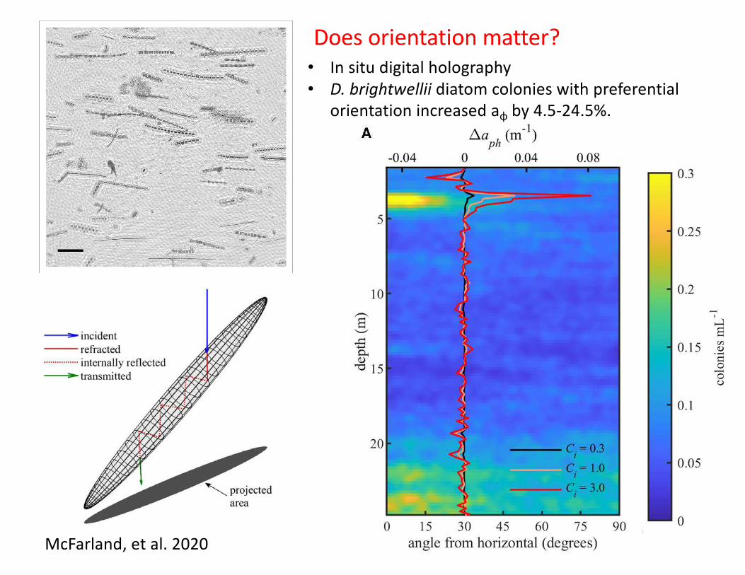
Does orientation matter?
McFarland et al. Diatom Orientation and Light Absorption
FIGURE 4 | Density (σt ), chlorophyll a concentrations (µg L−1), and backscatter (m−1) for each of three vertical profiles (A–C).
FIGURE 5 | Example extended depth of field image from the phytoplankton
thin layer in profile C showing predominantly horizontal orientation of diatom
colonies. Scale bar (lower left) represents 1 mm.
layer (Figure 5). The orientation distributions for each profile(Figure 6) revealed high concentrations of large (>100 µm),horizontally oriented particles at 3–4 m depth with angles
below ∼20 degrees. Particle concentrations were lower andorientation distributions were more uniform above and belowthe thin layer. As seen with backscatter, particle concentrationsdetermined from image analysis were also higher at depths >20m, especially in profile A (Figure 6A), most likely due to sinkingand flocculating detritus (Alldredge et al., 2002). Total modeledparticle concentrations for all orientations ranged from 5.45 to22.3 particles mL−1. The mean volume analyzed for estimatesof aph at each depth was 61.2 mL. This varied somewhat withthe descent rate of the instrument package (standard deviationof 24.2 mL).
Model results show absorption peaks in vertical profilescorresponding to the depth of the thin layer (Figure 7).Modeled aph (676 nm) at the thin layer peak for each Ci isshown in Table 1. Intracellular chlorophyll a concentrationshad a substantial impact on modeled values of aph whichincreased approximately five fold between the lowest andhighest values of Ci (0.3 and 3 kg m−3) at the thin layerpeak. A slight increase in modeled aph values at depths>20 m was seen in profile A (Figure 7), but no increasewas observed in measured apg at these depths despite higherbackscatter (Figure 4).
The effect of orientation on absorption, "aph, is shown inTable 1 and in Figure 6 overlaid on the observed orientationdistributions for each profile. We found positive modeled valuesof "aph for colonies within the thin layer. "aph also increasedwith increasing Ci. When compared to modeled and measuredabsorption (Table 1), values of "aph ranged from 4.5 to 24.5% ofmodeled aph and from 0.7 to 31% of measured apg . There was noincrease in "aph at depths >20 m in profile A despite indicationof some preferential horizontal orientation.
Frontiers in Marine Science | www.frontiersin.org 6 July 2020 | Volume 7 | Article 494
McFarland, et al. 2020
• In situ digital holography• D. brightwellii diatom colonies with preferential
orientation increased aɸ by 4.5-24.5%.
McFarland et al. Diatom Orientation and Light Absorption
FIGURE 2 | Illustration of the geometric optics model used to estimate
absorption by diatom colonies. Cells and colonies are represented by prolate
spheroids with major axes, minor axes, and orientation determined from image
analysis (Figure 1). Modeled ray paths originated from above and included 6
internal reflections. Absorption cross section was determined from the
decrease in radiant flux along internal ray paths (shown in red) and integration
over the vertically projected area.
A value of 0.014 m2 mg–1 was used for a∗ph, appropriate for thelarge coastal phytoplankton found in East Sound (Bricaud et al.,1995; Roesler and Barnard, 2013).
Vertical profiles of aph at 676 nm were modeled forphytoplankton populations in their measured orientations (aph)and in simulated random orientations (arph) by assigningrandomly generated angles to all spheroids. Random angles wereassigned five times and arph was determined as the mean over allrandomized orientations. We computed the parameter !aph asthe difference between aph and arph (!aph = aph − arph). !aph,therefore, represents the effect of the measured, non-randomorientation distribution on absorption. Positive values indicate anet increase in aph relative to random orientations while negativevalues indicate a net decrease.
2.6. Model ValidationAccuracy of the geometric optics model was assessed bycomparison with Lorenz-Mie theory for homogeneous spheresof various diameter and complex refractive index (Bohren andHuffman, 1998). The imaginary part of the complex refractiveindex (n′) was calculated according to Morel and Bricaud (1986):
n′ =acmλ
4πm
Where acm is the intracellular absorption coefficient atwavelength λ (676 nm) and m is the corresponding refractive
FIGURE 3 | Comparison of absorption efficiencies (Qa) at 676 nm calculated
with geometric optics (geo, solid lines) and Lorenz-Mie theory (mie, dashed
lines) for spheres of various size and intracellular chlorophyll content (Ci ).
index of sea water (1.3368) at a temperature of 12◦C andsalinity of 30 PSU (Quan and Fry, 1995). Model estimatesof Qa at 676 nm were compared for intracellular chlorophyllconcentrations between 0.1 and 4 kg m–3 and cell diametersranging from 2 to 400 µm (Figure 3). The geometric opticsmodel produced slightly smaller estimates of absorption thanLorenz-Mie theory. Comparison of model outputs showedthat absorption efficiencies varied by less than 2.5% betweenthe two models for this range of sizes and refractive indices.The largest difference between the models was found at highintracellular chlorophyll concentrations for 60 µm diameterspheres. Differences decreased with increasing particle size.
3. RESULTS
Vertical profiles of density, backscatter, and chlorophyll afor three separate casts revealed shallow thin layers of highphytoplankton biomass along the pycnocline (Figure 4). EDFimages reconstructed from in situ holographic video showedthese thin layers to be composed primarily of the colonialdiatom Ditylum brightwellii (Figure 5). Other less abundantchain forming diatoms included Eucampia zodiacus, variousspecies of Chaetoceros, Dactyliosolen fragillisimus, Skeletonemasp., Stephanopyxis turris, Leptocylindrus danicus, Cerataulinapelagica, and Pseudo-nitzschia sp. Phytoplankton samplescollected with a net tow and examined with a conventionalmicroscope confirmed these identifications. Backscatter profilesalso show an increase in non-algal or detrital particles at depths>15 m, most likely due to sinking detrital material and particleflocculation (Figure 4, Alldredge et al., 2002; Sullivan et al., 2005;McFarland et al., 2015).
Preferential horizontal orientation of long diatom chainswas clearly visible in EDF images acquired within the thin
Frontiers in Marine Science | www.frontiersin.org 5 July 2020 | Volume 7 | Article 494
McFarland et al. Diatom Orientation and Light Absorption
FIGURE 6 | Orientation distributions (bottom x-axis) for three profiles (A–C) and modeled change in absorption (!aph) due to orientation (top x-axis) at 0.3, 1.0, and
3.0 kg m−3 intracellular chlorophyll concentrations (Ci ). Color scale shows the concentration of colonies at a particular depth and orientation. Modeled !aph values are
the difference between measured and simulated random orientations.
FIGURE 7 | Modeled phytoplankton absorption coefficients (aph) at 0.3, 1.0, and 3.0 kg m−3 intracellular chlorophyll concentrations (Ci ) and measured total
absorption coefficients (apg) at 676 nm for three profiles (A–C).
4. DISCUSSION
The optical model used in this study showed an increasein absorption of 4.5–24.5% for populations of horizontallyoriented diatom colonies relative to random orientations.Computations were based on the measured orientation andsize distribution of a natural phytoplankton community,
and the modeled effects were repeated over three separateprofiles. Results suggest that horizontal orientation helpsmaximize light absorption by relatively large (>100 µmlength), high aspect ratio (length/width > 3) phytoplankton.This may allow horizontally oriented cells and colonies toachieve higher rates of photosynthesis and growth under lightlimited conditions.
Frontiers in Marine Science | www.frontiersin.org 7 July 2020 | Volume 7 | Article 494

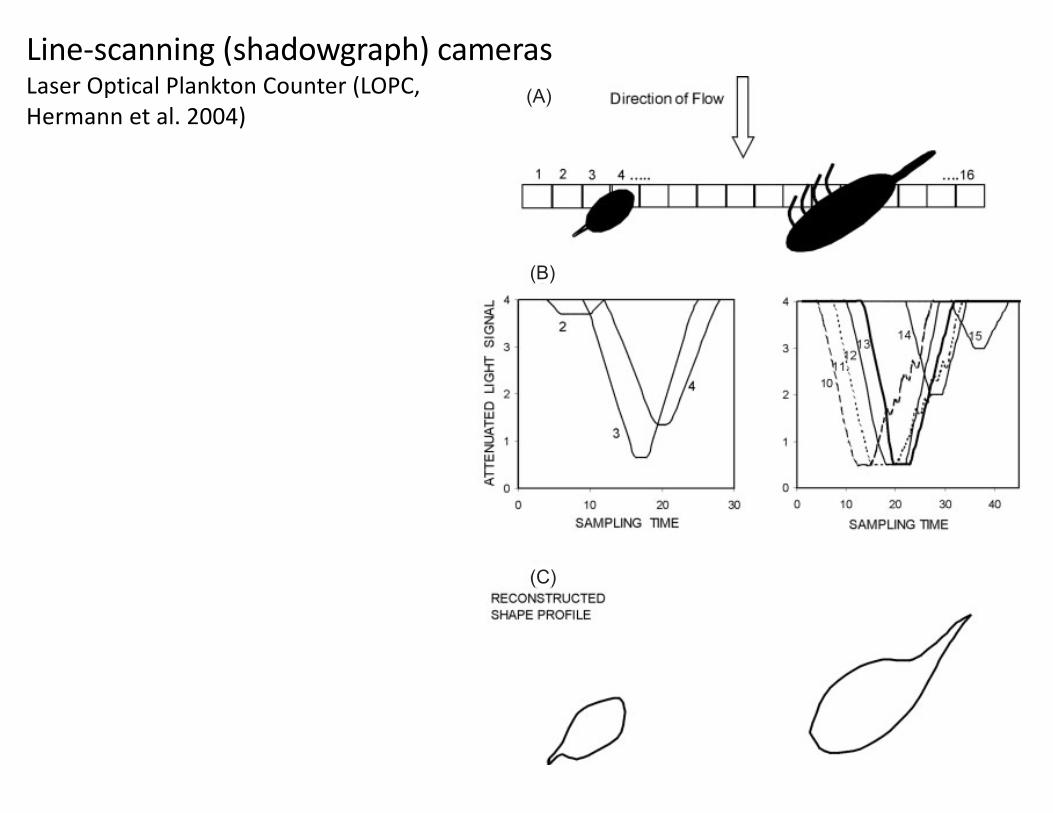
Line-scanning (shadowgraph) cameras
mapping of zooplankton distributions in the CaliforniaCurrent (Huntley et al., 1995).
The OPC measures and transmits the cross-sectionalarea of each particle passing through its beam and, as withall instruments, there are inherent limitations with its meas-urement capabilities. The most dominant is that of thecoincidence limit, that is, the density at which there is asignificant probability of two or more particles occurring inthe beam simultaneously. As a result, the multiple particlesare counted as one count and the size is presented as the sumof cross-sectional areas of all particles in the beam. In thecase of the OPC, coincidence became a problem at plank-ton density of !10 000m"3. Another limitation for the useris the lack of direct measurement of flow through the OPCtunnel. Even with recent technology advances, there is stillnot a suitable flow meter small enough in size that wouldeasily adapt to the existing OPC tunnel. As a result usershave adapted larger flow meters in the vicinity of the OPCor have simply used tow speed as a proxy for flow.
The new Laser-OPC (LOPC) has been under devel-opment and field testing at the Bedford Institute ofOceanography (Ocean Physics Division) since 1996with a preliminary report in Herman et al. (Herman et al.,1998). It was designed to resolve the limitations ofthe original OPC and also to provide further zooplank-ton identification capabilities by measuring the shapeprofiles of plankton larger than 1.5 mm (approximatespherical diameter). This paper describes the principlesof operation of the LOPC, its mechanical configuration,and the zooplankton parameters (e.g. size, shape, etc)that it measures. Data sampled regionally from ScotianShelf waters and the Gulf of St Lawrence will be shown
consisting of size distributions, shape profiles of largezooplankton such as Calanus spp. and euphausiids, andflow measurements. The deployment of the LOPC onvarious platforms and vehicles will be discussed.
LOPC OPERATING PRINCIPLESAND PHYSICAL DESCRIPTION
The operational principle of the LOPC is shown inFigure 1. A combination of laser diode and line genera-tor produces a diverging linear beam 1 mm in width.The beam is focussed by a cylindrical lens producing aparallel beam of 1 # 35 mm, subsequently reflected 90$
by a mirror and directed through an air–water interfacewindow into the sampling volume. At a selected distancefrom the window, a mirrored prism is used to redirectthe beam back to the window on a parallel path directlybelow the emerging beam. Based on a beam height of35 mm, the total frontal area occupied by the beam ina standard sampling tunnel is 70 # 70 mm. The micro-processor shown in Figure 1 does not represent a singlecomponent but rather a system consisting of a number ofmicroprocessors. The central unit processing is com-prised of (i) a digital signal processor (DSP—TexasInstruments, 200 MHz, 1600 MIPS) processing dataand algorithms, (ii) a programmable logic device(PLD—Cypress Semiconductor, in-circuit programm-able, 64 macrocell, 125 MHz) digitizing and multiplex-ing data from the photodiode, and (iii) a microprocessor(Persistor Instruments, CF1 module, 32 bit, 16 MHz)operating as a system manager (i.e. sensor integration,telemetry and data handling/management).
Fig. 1. The operating principle of the LOPC showing the formation of a ribbon-like laser beam of cross-section 1 # 35 mm. The region betweenthe window and prism (left hand side) represents the sampling volume. By doubling back the beam via a prism, we eliminate the need for a secondreceiver pressure case.
JOURNAL OF PLANKTON RESEARCH j VOLUME 26 j NUMBER 10 j PAGES 1135–1145 j 2004
1136
Dow
nloaded from https://academ
ic.oup.com/plankt/article/26/10/1135/1550119 by guest on 14 July 2021
Laser Optical Plankton Counter (LOPC, Hermann et al. 2004)
(v) measurement of flow speeds within the tunnel, and(vi) overall smaller physical size.
With the availability of new types of data from theLOPC, we see the potential for new development workin data interpretation beginning to arise. For example,the algorithms used to reconstruct shape profiles as thoseshown in Figures 7A and B need further developmentand data interpretation. Using the wide tunnel LOPC,antennae and appendages of copepods shown in Figure7A are greatly overestimated in their thickness and, as aresult, biomass determined from these shape profiles are
also overestimated. With LOPC data somewhat analo-gous to video imaging, there is also the need for thedevelopment of image recognition software that wouldprovide some taxonomic identification capabilities to theuser. The LOPC shape images are, of course, only intwo dimensions while animal orientation will result in aprojected area and not the full shape. However, thereare certain geometrical features that can be used, for
Fig. 12. The LOPC mounted on the inside of a plankton ring-net. A small CTD is mounted behind the LOPC and a TSK flowmeter is mountedbeside the LOPC sampling tunnel. This simple configuration is very useful for intercomparison of net samples with LOPC measurements.
Fig. 13. The LOPC mounted inside the towed fish of the MovingVessel Profiler (MVP). The fish is released and free-falls to about 250 m,is recovered again by a conductor cable, and re-released resulting incontinuous cycling while towed at 12–14 knots.
Fig. 14. The wide tunnel LOPC mounted on the undercarriage ofa Batfish vehicle towed at 8 knots. The wide tunnel processes higherwater volumes making it useful for sampling euphausiid layers.
JOURNAL OF PLANKTON RESEARCH j VOLUME 26 j NUMBER 10 j PAGES 1135–1145 j 2004
1144
Dow
nloaded from https://academ
ic.oup.com/plankt/article/26/10/1135/1550119 by guest on 14 July 2021
• Simple optics (linear diode array detector)
• Relatively large depth of field/sampling volume
• Limited particle image detail
In both cases of the LOPC and OPC, the ratiomeasured (particle area to photodiode element area)is approximately proportional to the particle area, how-ever, some deviation occurs since the light beam distri-bution across the photodiode possesses (i) a near-Gaussian shape, and (ii) some non-uniformities. Themajor change results from utilizing a smaller sensingelement of 1 mm2 in the LOPC as compared with theOPC whereby a lower size detection capability isobtained with the LOPC. Currently the lowest detectionthreshold is set at 100 mm (e.s.d.) for optimum per-formance with the LOPC, however, lower thresholdsof 50 mm have been tested also and may become opera-tional in the near future. In comparison, the lowestdetection limit of the OPC is 200–250 mm.
LOPC SIZE MEASUREMENTSAND INTERNAL CALIBRATION
The LOPC size measurement format of SEPs differsfrom that format of the OPC, in that the OPC presentsa size distribution linear with particle area whereas theLOPC presents a size distribution linear with particle
diameter (e.s.d.). The e.s.d. refers to that diameterderived by equating the area of a circle to the areameasured of an irregularly-shaped particle (i.e. a cope-pod). The calibration of e.s.d. versus LOPC-measuredarea is first performed by using a range of near-sphericalbeads which are passed through the light beam andmeasured. The resultant calibration of e.s.d. versusarea then becomes internally resident within the LOPCmicroprocessors. Following each measurement of a par-ticle area, the e.s.d. is calculated by the LOPC and acount incremented within a size interval or bin havinga size range encompassing that measured e.s.d.
The SEP size distribution is comprised of 128 bins intotal with a size range of 15 mm each and extending to amaximum of 1920 mm. All 128 bins and their appropriatecounts/bin are telemetered to surface every 0.5 s to pro-vide reasonable spatial resolution while towing at mostspeeds. Each transmission of 128 bins is immediately fol-lowed by a data line consisting of auxiliary instrumentdata, such as a CTD, providing the depth informationrequired by the user to locate vertically the size distribu-tions. Examples of SEP or small plankton distributionsmeasured by the LOPC are shown in Figure 6 illustratinga range of 100–1000 mm in ESD within bins of 15 mm.
In considering the cross-over region of SEP and MEPmeasurements of the LOPC, we consider the example inFigure 4B showing spherical particles ranging in sizebetween 1 and 2 mm. In examining the simple geometryof such particles passing over the multi-element photo-diode, there is a reasonable probability that the sphericalparticle of 1–2 mm e.s.d. will occupy three elementsduring its passage. For sizes on the high side of the1–2 mm range (i.e. 1.8 mm as shown in Figure 4B),the probability (of occupying three elements) is higher
(A)
(B)
(C)
Fig. 5. The principle of multi-element plankton (MEP) detection isshown for two plankton sizes. Both plankton pass over the detector in(A) and produce attenuated signal pulses in (B) with specific widths(time) and heights. The data group is transmitted from the probe to thesurface where reconstruction produces each shape profile shown in (C).
Fig. 6. The SEP diameter (e.s.d.) distribution sampled by the LOPCwhile mounted inside a ring-net and towed vertically. The peakbetween 100–200 mm corresponds to copepod eggs.
A. W. HERMAN, B. BEANLANDS AND E. F. PHILLIPS j LASER-OPC
1139
Dow
nloaded from https://academ
ic.oup.com/plankt/article/26/10/1135/1550119 by guest on 14 July 2021
Line-scanning (shadowgraph) cameras Laser Optical Plankton Counter (LOPC, Hermann et al. 2004)

H"+$I70)++"+4&!7()1-<4.)6(8&0)/$.)7&Y()^>,F)Y.,/S+6"'(0,+( Y;'&>(&)^S-,%;)5Y^YY^N)E+O%()'(#)*F>&'(#1)@AA4<
Cowen and Guigand In situ ichthyoplankton imaging system
127
(and its cousins) has been limited in the volume of water thatcan be sampled (e.g., the VPR is usually limited to a small rec-tangle to ensure sufficiently fine pixel resolution for resolvingsmall plankters, with a very narrow depth of field—resulting ina sample volume ranging from a few milliliters to 30 mL/frame[0.9 L s–1 at 30 frames s–1]; Davis et al. 2005). The drawback tothese systems is that this volume of sampled water is too smallto adequately quantify larger, but rarer plankton. Whereascopepods, and some invertebrate zooplankters, may exceeddensities of 1 to 10 individuals L–1, ichthyoplankton typicallyoccur at densities of ca. 0.01 to 0.001 individuals L–1. To morebroadly sample ichthyo- and other meso-zooplankters, othertechniques (e.g., OPC and SIPPER; Herman et al. 1992, Remsenet al. 2004, respectively) have involved imaging and/or count-ing plankters by size, as they pass through a narrow tube, anapproach that does not enable true in situ observations, andwhich can potentially distort fragile and highly mobile plank-ton into nonidentifiable shapes.
Our goal was to build on both existing knowledge (i.e.,previously designed systems) and hardware to develop a very-high-resolution towed digital imaging system capable of sam-pling water volumes sufficient to accurately quantify larvalfish In situ. We describe an imaging system, In situ ichthy-oplankton imaging system (ISIIS), that accommodates some ofthe problems associated with imaging relatively rare, albeitstill very small organisms In situ (i.e., without any indicationsof disturbance). This system is composed of several compo-nents: very-high-resolution imaging camera (line scan), back-lighting physics, high-throughput data transfer and storage,towed vehicle, and image analysis data processing. We focuson the physical system here, and leave the image analysiscomponent to a separate report, as it corresponds to a parallelresearch effort.
Materials and ProceduresPrototype overview—This camera system utilizes a combina-
tion of a light emitting diode (LED) light source, modified byplano-convex optics to create a collimated light field, whichbacklights a parcel of the water column and a high-resolutionline scanning camera (see Figure 1). With the application ofmirrors, the imaged parcel of water passes between the forwardportions of two streamlined pods (underwater [UW] housings)and thereby remains minimally affected by turbulence. Theresulting very-high-resolution image is of zooplankton in theirnatural position and orientation. When a sufficient volumeof water is imaged this way, then quantification of density,organism size, and fine-scale distribution is possible.
Lighting—We use lighting that involves shadow illumina-tion (Arnold and Nuttall-Smith 1974; Ortner et al. 1979, 1981).The focused shadowgraph technique allows for a long depthof field, not achievable with other lighting techniques such asdark field or simple backlighting. Moreover, this lightingscheme gives a very good contoured, as well as contrasted,image of small, transparent organisms such as zooplankton.
Because the light rays are directed toward the imaging sensorand not scattering off the actual filmed subject, the intensityof light required is extremely low compared with any otherlighting technique. This avoids the use of bright light sourcesthat may deter or otherwise compromise the behavior oforganisms. Moreover, a small, compact, vibration-resistantlight source such as LED can be used without the need to beoverpowered or strobed. This greatly simplifies the design and,in fact, makes it even more robust.
The system is composed of a plano-convex lens (150 mmdiameter and 586 mm focal length) creating a collimatedbeam of light through the volume of sampled water using a setof aluminum-coated mirrors (see Figure 1). Once the colli-mated beam of light passes through a second lens, it is refo-cused (Arnold and Nuttall-Smith 1974; Settles 2001) before itimpinges on the camera lens (Nikkor 85 mm). This makes thesystem economical in terms of light intensity, since almost allthe light entering the sampled volume hits the camera sensor.For our light source, we used LED technology, specifically a5 W 455 nm (blue) wavelength LED. Because this system doesnot require a large amount of light, this LED is suitable forobserving plankton in a relatively undisturbed environment.Moreover, this optical scheme makes the system telecentric,meaning that magnification is independent of distance fromthe camera to the specimen (Arnold and Nuttall-Smith 1974),thereby providing the opportunity to accurately measure sizeof zooplankters within the imaged volume.
Camera—For imaging, we used an 8-bit (256 grayscale), line-scan camera (DALSA P2-22-02k40). These cameras functionlike fax machines, departing from traditional area-scan CCD(charge coupled device) cameras. The camera creates a picture
Fig. 1. Light scheme using shadowgraph technique. Light passesthrough plano-convex lens, thereby establishing a collimated light beam.The advantages of this approach over other lighting techniques includehigh depth of field (20+ cm), telecentric image (magnification level notaffected by distance from object to the lens), and very sharp outlines oforganisms and internal structures (facilitates automated recognition).
Cowen and Guigand In situ ichthyoplankton imaging system
130
in the volume imaged and image resolution (see below) shouldgreatly improve this system’s capacity for fine-scale resolution ofichthyoplankton distribution and environmental interactions.
Beyond simple density estimates, continuous samplingallows parsing of data into very fine time/depth stanzas. Suchdata can then be plotted to examine fine-scale distributions inassociation with environmental measurements such as tem-perature, salinity, density, Chl a, and dissolved oxygen. For
our particular example, the water column in the upper 40 mof the core of the Florida Current is well mixed, and thereforefew fine-scale vertical features were observed. However, whenthe distribution of larvae with respect to their nearest neighborwas compared with random expectations, we saw evidence ofaggregation at very small scales (i.e., 2–4 m; Figure 7B).Although preliminary, this analysis demonstrates some of thepotential results possible with more extensive sampling and inmore vertically/horizontally stratified environments.
Fig. 4. In situ invertebrate zooplankters. 0–40 m depth, Florida current.Selected images of invertebrate plankton captured via ISIIS. Organismsare not scaled to each other in this composite image; sizes range from afew millimeters to several centimeters. A. Larvacean (Oikopleura sp.).B. Scyllarid lobster larva. C. Unidentified larval crustacean (?). D. Chaetog-nath. E. Copepod with eggs. F. Ctenophore. G. Ctenophore with feedingtentacles extended. H. Aggregate phase Thaliacean salp with reproduc-tive buds. I. Ctenophore (Velamen sp.). J. Pterotracheid heteropod.
Fig. 5. In situ cyanobacteria. Close-up of image of the cyanobacteria Tri-codesmium. Although very small (ca. 2–4 mm), its unique shape rendersthis organism easily discerned by the system.
Fig. 6. Raw image of zooplankton aggregation. Single 14 by 14 cmframe showing aggregation of similarly oriented crab zoea larvae.
Fig. 7. Quantitative comparisons. A. Comparison (mean and SD) oflarval fish sample densities from 1 m2 (150 µm mesh size) and 4 m2 (800 µmmesh size) MOCNESS nets versus the prototype ISIIS. Samples were com-pared over two depth bins, 0–25 m and 25–40 m. Note that samples weretaken in same area and time of year, but different years, so some variationmay be interannual variation. 1 m2 MOCNESS samples were not yet ana-lyzed for 25–50 m depth bin. B. Estimation of the degree of aggregationof larval fish at different spatial scales. The red line is expected proportionof fish if randomly distributed. Blue bars are observed data. Greater thanexpected co-occurrence of larvae at 2- to 4-m scales was observed.
! ]%$S)"'$&%)-';6">(&)L+"F;%)5MA)PI-)',)@?a);I-),+O)-6%%#<
! !8>">,S),+)+8-%$L%)"'$&%1)T$'&>"%)+$&'(>-;-)&"-'&0!
Overview
üTheory üInstrumentation examples (major types, emphasis
on systems in wide use)• Particle detection & classification• Challenges
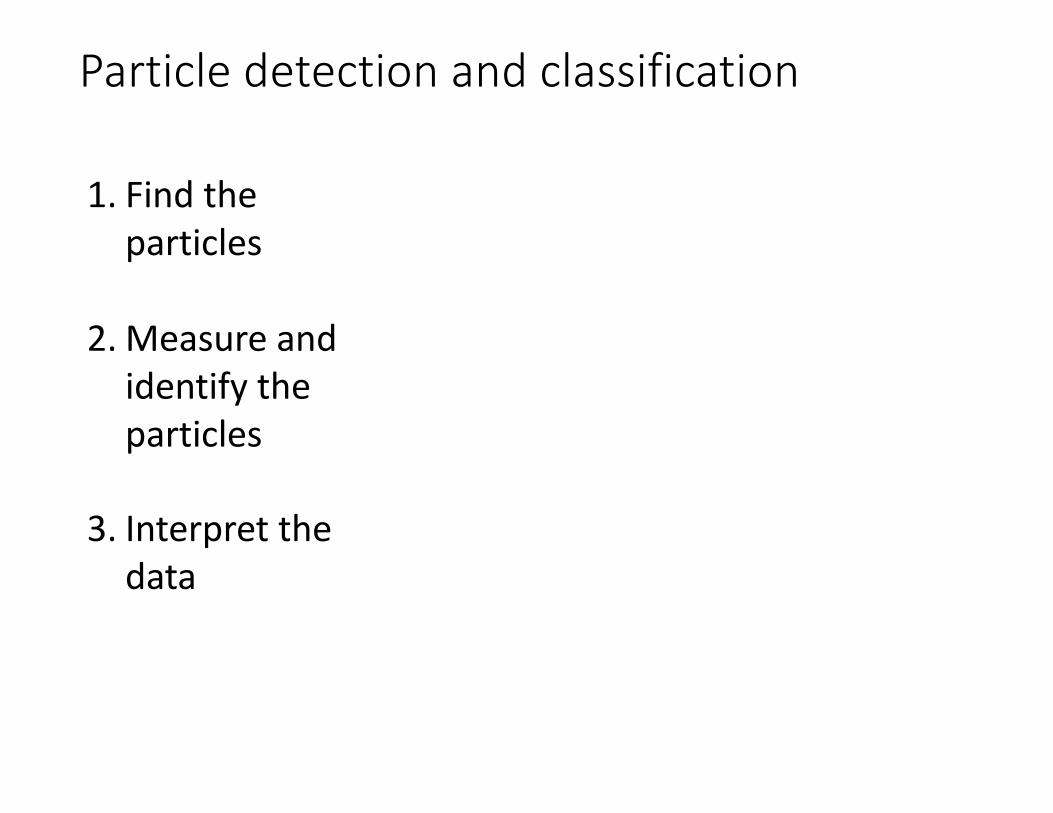
Particle detection and classification
1. Find the particles
2. Measure and identify the particles
3. Interpret the data

Particle detection and classification
11
189
Figure 1. Schematic illustration of image processing methods including a) detection of 190
particles, b) combination of multiple focal planes from the same field of view and collection 191
of particle measurements, and c) combination of flux measurements from optimal 192
magnification ranges. Processing steps for brightfield images are indicated by solid arrows 193
while processing of oblique images also included steps indicated by arrows with dashed 194
lines. 195
9011 32 362size (µm)
one field,one focal
plane
selected color
channelsremove
background
threshold
selectin-focusparticles
focal planes from same field
combine & remove duplicates
record measurements
extract particle images
c
a
b
maskedSobel filter
thresholding
greyscale
red
blue
sharpestedges
assignclassification
flux
(# m
-2d-1
µm-1
)
NE shelf breakPacific stations
combine optimal magnification ranges: 7×, 20×,40×/ 50×,
80×/ 115× size (µm)
detect particles as in panel a
highlightbrown pixels
.CC-BY-NC-ND 4.0 International licenseavailable under a(which was not certified by peer review) is the author/funder, who has granted bioRxiv a license to display the preprint in perpetuity. It is made
The copyright holder for this preprintthis version posted February 17, 2021. ; https://doi.org/10.1101/2021.02.16.431317doi: bioRxiv preprint
Figure, Durkin et al., in revision
1. Find the particles
2. Measure and identify the particles
3. Interpret the data

Segmentation: differentiating between background and particle
fmars-07-00564 July 20, 2020 Time: 20:39 # 5
Giering et al. Effects of Particle Detection Methods
TABLE 1 | Threshold algorithms.
Type Name Example Description and reference
Threshold (Reference) Otsu Finds threshold that minimizes the intra-class variance Ref: Otsu,1979
Threshold Isodata Takes an initial threshold and averages the pixels below and abovethe threshold. The averages of these two values are calculated.Threshold is incremented and the process is repeated until thethreshold is larger than the composite average Ref: Ridler andCalvard, 1978
Threshold Li Implements minimum cross entropy Ref: Li and Tam, 1998
Threshold Mean Uses the mean of gray levels as the threshold Ref: Glasbey, 1993
Threshold Minimum Assumes bimodal histogrammes Ref: Prewitt and Mendelsohn,1966
Threshold Triangle Uses a geometric method assuming a maximum peak (mode) nearone end of the histogram and searches toward the other end Ref:Zack et al., 1977
Threshold Yen Uses two criteria: the discrepancy between the thresholded andoriginal image, and the number of bits required to represent thethresholded image Ref: Yen et al., 1995
Edge Canny First smoothes the image using Gaussian convolution and thenhighlights regions with high first spatial derivatives (edges) using a2D gradient operator similar to Roberts Ref: Canny, 1986
Edge Roberts Performs 2D spatial gradient measurements by passing two 2 ⇥ 2convolution masks along the image Ref: Roberts, 1963
Edge Scharr Variation of Sobel algorithm Ref: Scharr, 2000
Edge Sobel Performs 2D spatial gradient measurements by performingconvolution between two 3 ⇥ 3 kernels and the image Ref: Sobeland Feldman, 1973
Histograms show the distribution of gray levels from 0 (black) to white (255) for the original image (left). Red line indicates the threshold identified by the algorithm, whichis applied to generate the thresholded image (right).
Frontiers in Marine Science | www.frontiersin.org 5 July 2020 | Volume 7 | Article 564
Giering et al, 2020aThreshold algorithms
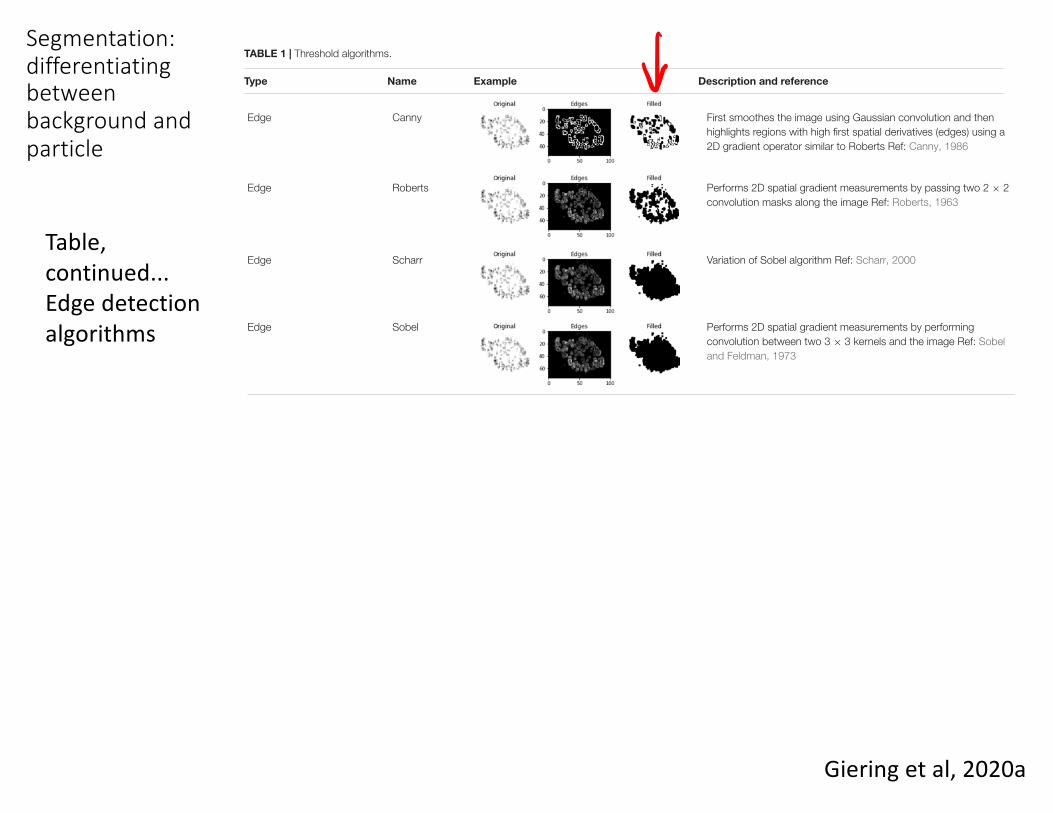
Segmentation: differentiating between background and particle
Giering et al, 2020a
fmars-07-00564 July 20, 2020 Time: 20:39 # 5
Giering et al. Effects of Particle Detection Methods
TABLE 1 | Threshold algorithms.
Type Name Example Description and reference
Threshold (Reference) Otsu Finds threshold that minimizes the intra-class variance Ref: Otsu,1979
Threshold Isodata Takes an initial threshold and averages the pixels below and abovethe threshold. The averages of these two values are calculated.Threshold is incremented and the process is repeated until thethreshold is larger than the composite average Ref: Ridler andCalvard, 1978
Threshold Li Implements minimum cross entropy Ref: Li and Tam, 1998
Threshold Mean Uses the mean of gray levels as the threshold Ref: Glasbey, 1993
Threshold Minimum Assumes bimodal histogrammes Ref: Prewitt and Mendelsohn,1966
Threshold Triangle Uses a geometric method assuming a maximum peak (mode) nearone end of the histogram and searches toward the other end Ref:Zack et al., 1977
Threshold Yen Uses two criteria: the discrepancy between the thresholded andoriginal image, and the number of bits required to represent thethresholded image Ref: Yen et al., 1995
Edge Canny First smoothes the image using Gaussian convolution and thenhighlights regions with high first spatial derivatives (edges) using a2D gradient operator similar to Roberts Ref: Canny, 1986
Edge Roberts Performs 2D spatial gradient measurements by passing two 2 ⇥ 2convolution masks along the image Ref: Roberts, 1963
Edge Scharr Variation of Sobel algorithm Ref: Scharr, 2000
Edge Sobel Performs 2D spatial gradient measurements by performingconvolution between two 3 ⇥ 3 kernels and the image Ref: Sobeland Feldman, 1973
Histograms show the distribution of gray levels from 0 (black) to white (255) for the original image (left). Red line indicates the threshold identified by the algorithm, whichis applied to generate the thresholded image (right).
Frontiers in Marine Science | www.frontiersin.org 5 July 2020 | Volume 7 | Article 564
Table, continued... Edge detection algorithms
fmars-07-00564 July 20, 2020 Time: 20:39 # 10
Giering et al. Effects of Particle Detection Methods
FIGURE 6 | Comparison of different threshold algorithms relative to Otsu. (A) Particle size (ESD in mm). (B) Average POC flux per particle (mg C m�2 d�1). Valuesare expressed as boxplots (see legend for Figure 5). Gray dashed lines indicate 0.5, 1, and 2 times Otsu value. Note the different y-axis scales. Colors showthreshold algorithm type as orange (reference algorithm Otsu), blue (binary), and green (edge detection). Based on all imaged particles (n = 6400).
FIGURE 7 | Flux profiles from deployment DY086-34 near South Georgiaaccording to the different threshold algorithms. Fluxes were calculated for allparticles as described in the methods and summed for each vignette. Fluxprofiles were binned at 1-m resolution and a running mean (n = 11) calculated.
South Georgia site) varied from 2.29 to 2.96 depending on theflux algorithm (Minimum and Sobel/Scharr, respectively).
We observed a large e�ect of algorithm choice on medianparticle size (ESD), POC concentrations, flux estimates, and fluxattenuation rate (“b parameter”) at all sites (Table 5).
Solidity and RoundnessObserved particles ranged in solidity from very looselyaggregated (S < 0.1) to solid (S > 0.9). The mediansolidity of the particle population was strongly dependenton the threshold algorithm (Figure 8). The highest mediansolidity was estimated by the binary algorithm Minimum,with a median solidity of 0.83. The edge detection algorithmsRoberts, Sharr and Sobel diagnosed high solidities with amedian of 0.48–0.56. Canny and the other binary algorithmscalculated median solidity values between 0.30 and 0.36. Thestatic thresholds below a gray value of 60 also diagnosedvery solid particles, but owing to their poor performance(>75% of analyzed vignettes were “empty”), these are notfurther discussed.
There was no consistent relationship between particle sizeand solidity, though the density plots suggest two loose clusters(Figure 9). The most prominent cluster comprised of particleswith a diameter of around 20 px (⇠88 µm) and a relatively lowsolidity (S⇠0.25). There was a second cluster of particles witha similar diameter but much rounder shape (R > 0.75). For allalgorithms, particles with an ESD of>30 px (⇠132µm) appearedto become less solid as they got larger.
We next investigated the roundness of particles accordingto the di�erent algorithms. The population median wassimilar for all binary (except Minimum) and edge detectionalgorithms, ranging from 0.36 to 0.42 (Figure 8). The Minimumalgorithm estimated particles to be rounder (median: 0.53),while the static thresholds above 60 estimated particles to
Frontiers in Marine Science | www.frontiersin.org 10 July 2020 | Volume 7 | Article 564
...Large relative variations in particle diameter depending on detection algorithm used

!"#$"%&'&()%*+,(--"."%&('&(%#+/"&0""%+/'12#.)3%,+'%,+4'.&(15"Sosik and Olson Phytoplankton image classification
208
simplified boundary with a combination of DIPUM functionsand custom algorithms. These detailed features include 1) thenumber of line segment ends on the blob perimeter (poten-tially indicative of spines, for instance); 2) relative cell widthnear the left and right edges compared to the midpoint (a pos-sible indicator for cells with distinctive ends such Ditylum spp.and Rhizosolenia spp.); 3) mean (absolute and relative to equiv-alent spherical diameter) and standard deviation of the distancesbetween the blob centroid and points along its perimeter; 4) the
number of concave and convex segments along the perimeter[see Loke and du Buf (2002) for development of this ideaapplied to diatom frustule characterization]; 5) symmetry met-rics based on the Hausdorff distance, a measure of how much2 shapes overlap, as applied to blobs compared with them-selves rotated 90 and 180 degrees and reflected along the lon-gitudinal centerline [e.g., see Fischer and Bunke (2002) forapplication to diatom frustules]; and 6) triangularity and ellip-ticity metrics specified by Rosin (2003) on the basis of the firstaffine moment invariant of Flusser and Suk (1993).
Various texture properties [e.g., contrast, smoothness, uni-formity, and entropy as specified by Gonzalez et al. (2004) andimplemented in the DIPUM toolbox] were determined onoriginal grayscale images, but only considering the pixelswithin the largest blob determined as described above. Inaddition, following the success of Hu and Davis (2005) withthis technique for zooplankton images, more detailed charac-terization of texture was included through calculation of gray-level co-occurrence matrices (MATLAB Image Processing Tool-box functions) for the original images. As individual features,we used statistics (mean and range of 4 properties: contrast,correlation, energy, and homogeneity) of 6 different gray-levelco-occurrence matrixes (pixel offsets of 1, 2, 4, 16, 32, and 64,each averaged for 4 angles, 0, 45, 90, and 135 degrees).
As indicators of geometric pattern, we also used the 7 invari-ant moments described by Hu (1962). These are independent ofobject position, size, and orientation and were determined withDIPUM algorithms. In the absence of evidence suggesting themost appropriate image processing stage for these features, wechose to calculate them for the original image, the blob image,and the simplified boundary (filled solid) image.
For the final features, we used digital diffraction pattern sam-pling (custom MATLAB code), previously shown to be effectivefor fingerprint and other pattern recognition problems(Berfanger and George 1999). We implemented a modified ver-sion of the method developed by George and Wang (1994),applied to the simplified boundary images. The approachinvolves calculation of the 2-dimensional power spectrum foran image, and then sampling it to determine the energy distri-bution across a pattern of wedges and rings radiating from theorigin. We used 48 rings and 50 wedges, each evenly distributedaround one-half of the power spectrum. To prevent low fre-quencies from dominating wedge signals, the portion of eachwedge near the origin (within an equivalent 15-pixel radius)was removed. Energy in each ring or wedge was normalized bythe total energy in the image to specify 98 features; 2 additionalvalues were included as features: the total energy in the powerspectrum and the ratio of energy near the center (within thelow frequency band eliminated from wedges) to the total.
As mentioned earlier, the final standard feature set for eachimage corresponds to a 210-element vector. The features forthe 3300-image training set then comprise a 210-by-3300 ele-ment matrix. Before proceeding with further steps involvedwith classifier development or application, all features were
Fig. 2. Image processing stages for example images from several cate-gories. The original grayscale images (A) are used for determining someclassification features, but different preprocessing is required for others(see Table 1). Calculation of phase congruency (B) in the original imagesis a critical step to produce robust edge detection (C). Through morpho-logical processing, edge images are converted into blob images (black andwhite) and then rotated (D). Finally, the first 10% of the Fourier descrip-tors are used to reconstruct a simplified blob boundary (E). Both the blobs(D) and the simplified boundaries (E) are used directly for feature calcula-tions. Each panel shows corresponding results for the same set of 5 images.
^+->0 '(#)D"-+(1)@AAM
Y=ER)'('"S->-)g 6/'-%).+(&$F%(.S).'".F"',>+()-,%6)5'",/+F&/).+;6F,',>+('""S)>(,%(->L%<)>;6$+L%-)6%$T+$;'(.%)+T),/$%-/+"#U8'-%#)%#&%)#%,%.,>+(

Particle identification – machine learning
Gonzàlez et al., 2019

14
Figure 2. Example micrograph collages of each sinking particle classification, including a) 233
aggregates, b) dense detritus, c) large loose fecal pellets, d) long cylindrical fecal pellets, e) 234
salp fecal pellets, f) Rhizaria, primarily Phaeodarians, g) phytoplankton cells, h) mini 235
pellets, i) short (ellipsoid or oval) fecal pellets. Scale bars in panels g and h: 100 µm, scale 236
.CC-BY-NC-ND 4.0 International licenseavailable under a(which was not certified by peer review) is the author/funder, who has granted bioRxiv a license to display the preprint in perpetuity. It is made
The copyright holder for this preprintthis version posted February 17, 2021. ; https://doi.org/10.1101/2021.02.16.431317doi: bioRxiv preprint
Particle identification –machine learning
Durkin et al., in revision
Figure: Classified particles collected in sediment traps
What if classes are not distinct from one another?

Giering et al. Sinking Particles From Optical Devices
BOX 2 | Equivalent Spherical Diameter (ESD) and Equivalent Circular Diameter (ECD).
ECD is calculated by rearranging the area of a particle into a circle and calculating its diameter (Figure 2). ECD and corresponding volume (V) can be calculated by
excluding holes (ECDexcl and Vexcl) or including holes (ECDincl and Vincl). Depending on the porosity of the particle, ECDexcl and Vexcl can be substantially smaller than
ECDincl and Vincl (respectively, 89 and 69% in our example). It is noteworthy that Vexcl might still overestimate the solid volume of a porous particle because of open
spaces in the particle that are not visible in an image.
ECD is often used synonymously with the equivalent spherical diameter (ESD). While ECD and ESD are similar and may be the same, they are practically calculated
differently with the former being derived from a 2D object and the latter from a 3D object. Different assumptions are used to allow this conversion, and these should
be stated clearly.
For particles with known geometry, e.g., cylindrical fecal pellets or certain phytoplankton, the transformation from the image area to the
particle volume can take advantage of this knowledge, and can even be corrected for the likely orientation of the particles relative to the
camera (Ebersbach and Trull, 2008; Ebersbach et al., 2011).
FIGURE 2 | Working steps to derive equivalent circular diameter (ECD) and volume (V) from the 2D image of a particle. Both metrics can be derived from the imaged
area (A). Care has to be taken whether holes are excluded (excl; top row) or included (incl; bottom row). Percentages at the bottom highlight the resulting differences
of our example (ratio between excluded over included).
size is in principle simple, however, in reality very complicatedbecause of the complex shapes of marine particles, such ascopepods with their legs and antennae, twisted diatom chainswith their spines, radiolarians with delicate spikes, aggregatesand feeding structures with complex shapes and empty cavities,or exopolymer particles, which are often undetected owing totheir transparency. Not all imaging systems can resolve thenecessary detail to capture such complex structures. Moreover,most imaging devices take a 2D image, which can substantiallymisrepresent the true size and shape of the original 3D particle.
For many devices with a relatively large depth of field, suchas the Video Plankton Recorder, the z-position of a particle isunknown,meaning that the true size is unknown: A small particleclose to the camera can have the same apparent size as a largeparticle further away (Figure 3). This imprecision is, however,likely averaged out over sufficient data provided that particles areilluminated consistently regardless of their z-position; i.e., smallparticles are as likely detected close to the camera than furtheraway. For shadowgraph systems, the imaging of silhouettes using
collimated light ensures that a particle is always imaged at thesame size, regardless of how close it is to the camera (Cowen andGuigand, 2008; Ohman et al., 2019). Alternatively, a telecentriclens configuration can be used. In particle-rich environments,overlapping of objects might become an additional problem fordevices with a large depth of field (Figure 3). Problems mightalso arise when only a small part of a larger particle is capturedor illuminated, leading to a potential underestimation of particlesize. Diffusion of light as it travels through the water from theparticle to the sensor can cause a “halo” effect in which smallparticles appear larger than they really are. This effect can becorrected for with a size specific conversion factor between pixelsand size (Picheral et al., 2010).
Estimating the absolute size of a particle using optical deviceswill likely always remain a challenge owing to the technicallimitations and overall assumptions of the different methods. Abig step forward to making data more comparable is increasedtransparency and standardization in data acquisition, analysisand description. We therefore recommend the following:
Frontiers in Marine Science | www.frontiersin.org 8 February 2020 | Volume 6 | Article 834
Computing particle volume (or carbon) from image area
Giering et al., 2020b
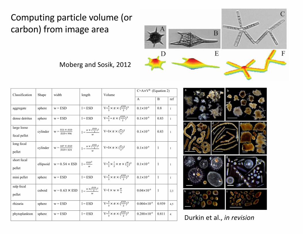
6� � � � � � � � � � � � � � � � � � � � � � � � � � � � � � � � � � � � � � � � � � � � � � � � � � � � � � � � � � � � � � � � � � � � � � � � � � � � � � � � � � � � � � � � � � � � � � � � ? � � � � � � �� � � � � � � % � � � � � � � � � � � � � � � � � � � � � � � � � � � � � � F� � G � � � � � � � � � �� � � � � � � � � � � � � � � � � � � � � � � � � � � � � � � � � � � � � � � � � � � � �� � � � � � � � � � � � � � � � � � � � � � � � � � � � � � � � � � � � � � � � � � � � � � � � � � �� � � � � � � � � � � � � � � � � � � � � � � � � � � � � � � � � � � � � � � � + � � ! " # � - � � � 9 * � � 8 �� � � � � � � � � � � � � � � � � � � � � � � � � � � � � � � � � � � � � � � � � � � � � � � � � � � � � � � � � � � F� � � G � � � � � � � � � � � � � � � � � � � � � � � � � � � � � � � � � � 7 C
� *
� � � � � $ % � � � � � � � � � � � � � � � � � � � � � � � � � � � � � � � � � � � �� � � � � � � � � � � � � � � $ % � � � � � � � � � � � � � � � � � � � � � � � � � � �
� � � � � � � � � � � � � � � � � � � � � � � � � � � � � � � � � � � � � � � � � - � � � ' * � � � � � � �� � � � � � � � � � � � � � � � � � � � � � � � � � � � � � � � � � � � � � � � � � � � � � � �� � � � � � � � � � � � � � � � � � � � � � � � � � � � � � � � � � � � � � � � �� � � � � � � � � � � � � � � � � � � � � � � � � � � � � � � � � � � � � � � * � � � � � � � � �� � � � � # � � � � � � � � � � � � � � � � � � � � � � � � � � � � � � � � � � � � � � � � � � � � � � �� � � � � � � � � � � � � � � � � � � � � � � � � � � � � � � � � � � � 8 � � � � � � � � � � �� � � � � � � � � � � � � � � � � � � �
- � � � � � � � � � � � � � � � � � � � � � � � � � � � � � � � � � � � � � � � � � � � � � � � �� � � � � � � � � � � � � � � � � � � � � � � � � � � � � � � � � � � � � � � � � � � � � � � � � �� � � � � � � � � � � � � � � - � � � " � * � � $ % � � � � � � � � � 5� � � � � � � � � � � � � �� � � � � � � � � � � � � � � � � � � � � � � � � � � � � � � � � � � � � � � � � � � � � � � � � � � � � � � � � � � � � � � � � � � � � � � � � � � � � $ � � � � � � � � � � � � � � � � � � � � � & # � � � � � � � � � � � � � � � � � � � � � � � � � � � � � � � � � � � �� � � � � � � � � � ! " � � � � � � & D+ � � /� � & � � � � � � � � � � � � � � � � � � � � � � � � � �� � � � � � � � � � � � � � � � � � � � � � � � � � � � � � � � � � � � � � � � � �
� + *
� � � � � � � & � � � � � � � � � � �
� 4 *
���
� �= !! �
��
�
�+
��
�
���
+ +
� � � � � � � � � � � � � � � � � � � � � � � � � � � � � � � � � � � � � � � � � �
� � %
� � � � � � 1 � � � � � � � � � � � # � � � � " � � � � � � � < � " � � � � � � � � � � � � � � � � � � � �� � � " � � ) � � � � � � � = � � � � " � � � � � � � � � � � � # � � � � � � � B� � � � � � � � � � � � � � � �� � " � � � < # � � � � � � � � � � � � % � � � � + % � � " � � � � � � % � � � � # � � � � B� � � �� � � � � , � � � � � � � � � � � � � � � � � � < � " � � � � � � � � � % � " � � � + � � � � , � � � �� � � � ! � � � � � � < � " � � � � � � � � % � � � � % � > � + � � � � � " � � � � � � , � � � � � � � �% � � � � � � � � � � � � � � � � �
� � � � � � 2 � � � " � � � � # � � � 6 2 ? � � � � � � � � � � @ � � � � � � � � � � � # � � � � � � " � � �� � � � � % � � � � � " � � � � � � � � " � � � � � � � � � < � " � � � � � � � � � % � " � � � � � � � � � � / � � � � � � � � � � " � � � � � � " � � � � # � � � � � � � � � � � � � � # # � � � � � � � �< � " � � � + � � � � � � � � � � , # � � � � � � � � � � � � � � " � � � � + � � # � � � � � � , �
� � � � � � + � � . � � , � = � � � � � � � � � � � � � � � � � � � # � � � � � � � + 2 � � � ) , � � � � � � � � � " � � � � � � � � � � � � � � � � � � ? � � � � � � � � � � @ # � � � � + � � 2 , � � � � � � � � � � � + . �� , � � � � � � � � � � + � � ) , � � � � � � � � � � � � � � � 1 � � � � � 6 � 2 � � � � " � � � � � � � � � � � � � � � � � � � � � � � � � � � " � � � � � � � " � � � � � � � � � � � � � " � � % � > � � � � � � � � � � � � � �� � � � � � % � � � " � � � � � � � � � � � � � � � � � " � % � � � � � � � � � � � � � � � � �
B+8%$&)'(#)^+->01)@A2@
! "#!
!"#$%&'(&)**+,-./01*&"12&%3+"./01*&+*%2&.0&,02%$&.4%&-"5./6+$".%&057"1/6&6"5#01&601.%1.&$%$!
08&%"64&-"5./6$%&.9-%(&&:"5",%.%5*&805&%3+"./01&'&;%5%&+*%2&850,&<"5/0+*&5%8%5%16%&*.+2/%*=&$%&!
5%8&>=&.4/*&*.+29?&'=&@/$<%5&"12&A5+$"12&B>CD>E?&F=&G<%5*%1&%.&"$(&B'H>IE?&J=&K%12%1LM%+%5&$%'!
"12&N%**"52&B'HHHE?&O=&@.+P%$&%.&"$(&B'H>DE(&Q@MR%3+/<"$%1.&*-4%5/6"$&2/",%.%5(&$%(!
!"#$$%&%'#(%)*+ ,-#./+ 0%1(-+ "/*2(-+ 3)"45/+!67!38+++9:;4#(%)*+<=+
7+ 8+ >/&+
#22>/2#(/+ $.-/>/+ 0+6+:,?+ "+6+:,?+ 36"# ! $ ! %
&'() *
#++ @AB!B@CD+ @AE+ B+
1/*$/+1/(>%(4$+ $.-/>/+ 0+6+:,?+ "+6+:,?+ 36"# + $ ! %
&'() *
#+ @AB!B@CD+ @AEF+ B+
"#>2/+"))$/+
&/'#"+./""/(+'G"%*1/>+ 0+6+
,,#-!-&'(&'(.-//0 + "+6+
1-!-%2345 *5
6 + 36"! $ ! %6)*)+ @AB!B@CD+ @AEF+ B+
")*2+&/'#"+
./""/(+'G"%*1/>+ 0+6+
789-!-&'(&'(.-")" + "+6+
1-!-%2345 *5
6 + 36"! $ ! %6)*)+ @AB!B@CD+ B+ B+
$-)>(+&/'#"+
./""/(+/""%.$)%1+ 0+6+@: ;< ! =>?+ "+6+
&'(56 + 36
"# !
@) ! $ ! %
6)*)+ @AB!B@CD+ B+ B+
5%*%+./""/(+ $.-/>/+ 0+6+:,?+ "+6+:,?+ 36"# ! $ ! %
&'() *
#+ @AB!B@CD+ B+ B+
$#".+&/'#"+
./""/(+'4H)%1+ 0+6+@: AB ! =>?+ "+6+
1-!%2345 *5
6 + 36"+!+0+! 6" + @A@I!B@CD+ B+ <JF+
>-%K#>%#+ $.-/>/+ 0+6+:,?+ "+6+:,?+ 36"# ! $ ! %
&'() *
#+ @A@@I!B@CD+ @ADFD+ IJL+
.-G()."#*M()*+ $.-/>/+ 0+6+:,?+ "+6+:,?+ 36"# ! $ ! %
&'() *
#+ @A<EE!B@CD+ @AEBB+ I+
+$%)!
N-/+!"#$%$&'(%$)$%$&'+&4*'(%)*+%*+.G(-)*+0#$+4$/1+()+&%*1+(-/+O#"4/$+)&+7+#*1+8+&)>+.#>(%'"/+$%#!
'#(/2)>%/$+%*+(-/+&%>$(+$%P+>)0$+)&+N#H"/+<+(-#(+2#O/+(-/+H/$(+&%(+()+")2+(>#*$&)>5/1J+H4"M+'#>H)*+$%%!
&"4P/$+5/#$4>/1+%*+(>#.+(4H/$A++Q*+(-/+&%((%*2+.>)'/$$J+(-/+$#5/+O#"4/+)&+7+0#$+#$$45/1+&)>+#""+$%P+$%*!
)&+(-/$/+.#>(%'"/+'#(/2)>%/$+#*1+86B+0#$+#$$45/1+&)>+#""+')5.#'(+&/'#"+./""/(+'#(/2)>%/$+9")*2J+$*+!
$-)>(J+5%*%=A++,-#>/1+8+O#"4/$+0/>/+#$$45/1+&)>+1/*$/+1/(>%(4$+#*1+"#>2/J+"))$/+&/'#"+./""/(+#*1+#+$*"!
.CC-BY-NC-ND 4.0 International licenseavailable under a(which was not certified by peer review) is the author/funder, who has granted bioRxiv a license to display the preprint in perpetuity. It is made
The copyright holder for this preprintthis version posted February 17, 2021. ; https://doi.org/10.1101/2021.02.16.431317doi: bioRxiv preprint
J-/63*"+4&6).*"0;$&K-;3/$&!-.&0).=-+8&,.-/&"/)4$&).$)
\F$0>()%,)'"?1)&"-.)2&'&3"
! "#!
!"#$%&'()'*+,-./&'-"0%1#%,.2'01//,#&3'14'&,02'3"56"5#'.,%7"0/&'0/,33"4"0,7"158'"50/$9"5#',:'$%%!
,##%&#,7&38';:'9&53&'9&7%"7$38'0:'/,%#&'/113&'4&0,/'.&//&738'9:'/15#'0</"59%"0,/'4&0,/'.&//&738'&:'$%#!
3,/.'4&0,/'.&//&738'4:'=2">,%",8'.%"-,%"/<'?2,&19,%",538'#:'.2<71./,56715'0&//38'2:'-"5"'$%&!
.&//&738'":'321%7'@&//".31"9'1%'1A,/:'4&0,/'.&//&73)''B0,/&';,%3'"5'.,5&/3'#',59'2C'DEE'µ-8'30,/&'$%'!
.CC-BY-NC-ND 4.0 International licenseavailable under a(which was not certified by peer review) is the author/funder, who has granted bioRxiv a license to display the preprint in perpetuity. It is made
The copyright holder for this preprintthis version posted February 17, 2021. ; https://doi.org/10.1101/2021.02.16.431317doi: bioRxiv preprint

Particle detection and classification
11
189
Figure 1. Schematic illustration of image processing methods including a) detection of 190
particles, b) combination of multiple focal planes from the same field of view and collection 191
of particle measurements, and c) combination of flux measurements from optimal 192
magnification ranges. Processing steps for brightfield images are indicated by solid arrows 193
while processing of oblique images also included steps indicated by arrows with dashed 194
lines. 195
9011 32 362size (µm)
one field,one focal
plane
selected color
channelsremove
background
threshold
selectin-focusparticles
focal planes from same field
combine & remove duplicates
record measurements
extract particle images
c
a
b
maskedSobel filter
thresholding
greyscale
red
blue
sharpestedges
assignclassification
flux
(# m
-2d-1
µm-1
)
NE shelf breakPacific stations
combine optimal magnification ranges: 7×, 20×,40×/ 50×,
80×/ 115× size (µm)
detect particles as in panel a
highlightbrown pixels
.CC-BY-NC-ND 4.0 International licenseavailable under a(which was not certified by peer review) is the author/funder, who has granted bioRxiv a license to display the preprint in perpetuity. It is made
The copyright holder for this preprintthis version posted February 17, 2021. ; https://doi.org/10.1101/2021.02.16.431317doi: bioRxiv preprint
Figure, Durkin et al., in revision
1. Find the particles
2. Measure and identify the particles
3. Interpret the data
Take-homes
• Imaging techniques provide important information about particle processes, validation for ocean color models• Needs for the future: standards; shared details of
image analysis methods; classification tools• Collaboration across groups, funding sources,
international community