F Fermi National Accelerator Laboratory

FERMILAB-Conf-98/344

Particle-Beam Approach to Collective Instabilities–Application toSpace-Charge Dominated Beams

K.Y. Ng and S.Y. Lee

Fermi National Accelerator LaboratoryP.O. Box 500, Batavia, Illinois 60510

November 1998

Published Proceedings of the 16th Advanced ICFA Beam Dynamics Workshop on Nonlinear and

Collective Phenomena in Beam Physics, Arcidosso, Italy, September 1-5, 1998

Operated by Universities Research Association Inc. under Contract No. DE-AC02-76CH03000 with the United States Department of Energy

Disclaimer

This report was prepared as an account of work sponsored by an agency of the United States

Government. Neither the United States Government nor any agency thereof, nor any of

their employees, makes any warranty, expressed or implied, or assumes any legal liability or

responsibility for the accuracy, completeness, or usefulness of any information, apparatus,

product, or process disclosed, or represents that its use would not infringe privately owned

rights. Reference herein to any speci�c commercial product, process, or service by trade

name, trademark, manufacturer, or otherwise, does not necessarily constitute or imply its

endorsement, recommendation, or favoring by the United States Government or any agency

thereof. The views and opinions of authors expressed herein do not necessarily state or re ect

those of the United States Government or any agency thereof.

Distribution

Approved for public release; further dissemination unlimited.

Copyright Noti�cation

This manuscript has been authored by Universities Research Association, Inc. under con-

tract No. DE-AC02-76CHO3000 with the U.S. Department of Energy. The United States

Government and the publisher, by accepting the article for publication, acknowledges that

the United States Government retains a nonexclusive, paid-up, irrevocable, worldwide license

to publish or reproduce the published form of this manuscript, or allow others to do so, for

United States Government Purposes.

Particle-Beam Approach toCollective Instabilities — Applicationto Space-Charge Dominated Beams

K.Y. Ng

Fermi National Accelerator Laboratory,∗ P.O. Box 500, Batavia, IL 60510

S.Y. Lee

Physics Department, Indiana University, Bloomington, IN 47405

Abstract. Nonlinear dynamics deals with parametric resonances and diffusion. Thephenomena are usually beam-intensity independent and rely on a particle Hamiltonian.Collective instabilities deal with beam coherent motion, where the Vlasov equation isfrequently used in conjunction with a beam-intensity dependent Hamiltonian. We ad-dress the questions: Are the two descriptions the same? Are collective instabilities theresults of encountering parametric resonances whose driving force is intensity depen-dent? We study here the example of a space-charge dominated beam governed by theKapchinskij-Vladimirskij (K-V) envelope equation [1]. The stability and instabilityregions as functions of tune depression and envelope mismatch are compared in thetwo approaches. The study has been restricted to the simple example of a uniformlyfocusing channel.

I INTRODUCTION

Traditionally, the thresholds of collective instabilities are obtained by solvingthe Vlasov equation for collective motion. The modes of instabilities are describedby the set of orthonormal eigenfunctions of the characteristic equation and thecorresponding complex eigenvalues give the initial growth rates.

The beam dynamics of the Vlasov equation derives from a Hamiltonian that in-cludes wakefields. The unperturbed beam distribution function is computed underthe influence of the mean field. The perturbative distribution function is obtainedby solving the Vlasov equation, which is often linearized so that the collectiveeigenmodes can be determined.

The nonlinear Hamiltonian can generally be decomposed into an unperturbedpart, H0, and a perturbation H1. The unperturbed Hamiltonian is derived fromthe external forces such as the quadrupoles, rf focusing potential, the space-chargemean-field potential, and the potential-well distortion due to low-frequency com-ponents of the wakefields.

The perturbation H1 can arise from nonlinear magnetic fields, high-frequencywakefields, etc. It may have a time-independent component, for example, the

∗) Operated by the Universities Research Association, under contracts with the US Departmentof Energy.

2

part involving the nonlinear magnetic fields, that gives rise to the dynamical aper-ture limitation of the dynamical system. On the other hand, it may also have atime-dependent component, which includes the effects of wakefields and producescoherent motion of beam particles. The harmonic content of the wakefields dependson the structure of accelerator components. If one of the resonant frequencies ofthe wakefields is equal to a fractional multiple of the unperturbed tune of H0, in-cluding the mean-field potential, a resonance is encountered and coherent particlemotion is introduced. This may result in a runaway situation such that collectiveinstability is induced.

Experimental measurements indicate that a small time dependent perturbationcan create resonance islands in the longitudinal or transverse phase space and pro-foundly change the bunch structure [2]. For example, a modulating transversedipole field close to the synchrotron frequency can split up a well-behaved bunchinto beamlets. Although these phenomena are driven by a beam-intensity indepen-dent source, they can also be driven by the space-charge force and/or the wakefieldsof the beam which are intensity dependent. Once perturbed, the new bunch struc-ture can further enhance the wakefields inducing even more perturbation to thecirculating beam. Experimental observation of hysteresis in collective beam in-stabilities seems to indicate that resonance islands have been generated by thewakefields.

For example, the Keil-Schnell criterion [3] of longitudinal microwave instabilitycan be derived from the concept of bunching buckets, or islands, created by theperturbing wakefields. Particles of the beam will execute synchrotron motion insidethese buckets leading to growth in the momentum spread of the beam. In fact,the collective growth rate is exactly the angular synchrotron frequency inside thesebuckets. If the momentum spread of the beam is much larger than the bucketheight, only a small fraction of the particles in the beam will be affected andcollective instabilities will not occur. This mechanism has been called Landaudamping.

As a result, we believe that the collective instabilities of a beam can also betackled from a particle-beam nonlinear dynamics approach, with collective insta-bilities occurring when the beam particles are either trapped in resonance islandsor diffuse away from the beam core because of the existence of a sea of chaos. Theadvantage of the particle-beam nonlinear dynamics approach is its ability to un-derstand the hysteresis effects and to calculate the beam distribution beyond thethreshold condition. Such a procedure may be able to unify our understanding ofcollective instabilities and nonlinear beam dynamics.

In this work, the stability issues of a space-charge dominated beam in a uniformlyfocusing channel are considered as an example. In Sect. II, the Hamiltonian formu-lation of the envelope equation is reviewed. In Sect. III, we present a brief accountof the collective-motion approach as studied by Gluckstern, Cheng, Kurennoy, andYe [4], using the Vlasov equation. For the particle-beam nonlinear dynamic ap-proach, we start with the particle Hamiltonian in Sect. IV, where the particle tuneis computed in the presence of beam-envelope oscillations with and without mis-

3

match. Section V is devoted to parametric resonances, where beam stability isinvestigated as a function of the space-charge perveance and beam envelope mis-match. In Sec. VI, beam particles having nonzero angular momentum are included.Finally, in Sec. VII, conclusions are given.

II ENVELOPE HAMILTONIAN

First, the envelope Hamiltonian is normalized to unit emittance and unit period.In terms of the normalized and dimensionless envelope radius R, together with itsconjugate momentum P , the Hamiltonian for the beam envelope in a uniformlyfocusing channel can be written as [5,6]

He =1

4πP 2 + V (R) , (2.1)

with the potential

V (R) =µ2

4πR2 − µκ

πlnR

R0+

1

4πR2, (2.2)

where µ/(2π) is the unperturbed particle tune, κ = Nrcl/(µβ2γ3) plays the roleof the normalized space-charge perveance, N is the number of particles per unitlength having the classical radius rcl, and β and γ are the relativistic factors of thebeam. The normalized K-V equation then reads

d2R

dθ2+(µ

2π

)2

R =2µκ

4π2R+

1

4π2R3, (2.3)

The radius R0 of the matched beam envelope or core is determined by the lowestpoint of the potential; i.e., V ′(R0) = 0, or

µR20 =√κ2 + 1 + κ =

1√κ2 + 1− κ

. (2.4)

From the second derivative of the potential, the small amplitude tune for envelopeoscillations is therefore

νe =2µ

2π

[1− κ

(√κ2 + 1− κ

)]1/2−→

2µ

2πκ→ 0

√2µ

2πκ→∞

(2.5)

For a mismatched beam, R varies between Rmin and Rmax. To derive the tuneof the mismatched envelope, it is best to go to the action-angle variables. Theenvelope action can be computed from the envelope Hamiltonian via

Je =1

2π

∮PdR . (2.6)

4

The envelope tune is then

Qe =dEedJe

= νe + αeJe + · · · , (2.7)

where Ee is the Hamiltonian value of the beam envelope, and the detuning αe,defined by

He = νeJe + 12αeJ

2e + · · · , (2.8)

is computed to be

αe =3

16π3R40ν2e

(µκ +

5

R20

)− 5

48π5R60ν4e

(µκ +

3

R20

)2

+ · · · . (2.9)

To obtain the envelope tune for large mismatch, one must compute numericallythe action integral to obtain

Qe =dEedJe

= 2π

[∮∂P

∂EedR

]−1

, (2.10)

The envelope tune is plotted in Fig. 1 as a function of the maximum enveloperadius Rmax, which for small mismatch is related to the envelope action Je by

R = R0 +(Jeπνe

)1/2

cosQeθ . (2.11)

FIGURE 1. Envelope tune Qe versus envelope mismatch Rmax/R0 for various space-chargeperveance κ. Notice that Qe is represented by νe at Rmax/R0 = 1 when the beam envelope ismatched.

5

III COLLECTIVE-MOTION APPROACH

Gluckstern, Cheng, Kurennoy, and Ye [4] have studied the collective beam sta-bilities of a space-charge dominated K-V beam in a uniformly focusing channel.The particle distribution f is separated into the unperturbed distribution f0 andthe perturbation f1:

f(u, v, u, v ; θ) = f0(u2 + v2 + u2 + v2) + f1(u, v, u, v ; θ) , (3.1)

where u and v are the normalized transverse coordinates which are functions of the‘time’ variable θ. Their derivatives with respect to time are denoted by u and v.The unperturbed distribution

f0(u2 + v2 + u2 + v2) =I0

v0π2δ(u2 + v2 + u2 + v2 − 1) (3.2)

is the steady-state solution of the K-V equation (2.3) and is therefore time-independent. In the notation of Gluckstern, Cheng, Kurennoy, and Ye, I0 is theaverage beam current and v0 the longitudinal velocity of the beam particles. Theperturbed distribution generates an electric potential G, which is given by thePoisson’s equation

∇2G(u, v, θ) = − 1

ε0

∫du∫dvf1(u, v, u, v ; θ) , (3.3)

so that the Hill’s equations in the two transverse planes become

u+ u = − eβ

m0v20ε

∂G

∂u, v + v = − eβ

m0v20ε

∂G

∂v, (3.4)

where ε stands for the transverse emittance of the beam and m0 the rest mass ofthe beam particle.

For small perturbation, the perturbation distribution is proportional to thederivative of the unperturbed distribution. This enables us to write

f1(u, v, u, v; θ) = g(u, v, u, v; θ)f ′0(u2 + v2 + u2 + v2) . (3.5)

Substituting into the linearized Vlasov equation, we obtain

∂g

∂θ+ u

∂g

∂u+ v

∂g

∂v− u∂g

∂u− v∂g

∂v=

2eβ

m0v20ε

[u∂G

∂u+ v

∂G

∂v

]. (3.6)

Noting that the potential G is a polynomial, Gluckstern, et. al. are able to solvefor g and G consistently in terms of hypergeometric functions. Thus a series oforthonormal eigenmodes are obtained for the perturbed distribution with theircorresponding eigenfrequencies. These modes are characterized by (j,m), where jis the radial eigennumber and m the azimuthal eigennumber.

For the azimuthally symmetric modes, m= 0. The (1,0) is the breathing modeof uniform density at a particular time. The (2,0) mode oscillates with a radial

6

FIGURE 2. Beam stability plot versus particle tune depression η and beam envelope mismatch.The stability region for the (2,0) mode is enclosed by the solid curve, that for the (3,0) modeby the dashed curve, and that for the (4,0) mode by the dot-dashed curve. (Reproduced fromRef. 4).

node between R = 0 and R = R0 so that the density becomes nonuniform. Thehigher modes are similar, with the (j, 0) having j − 1 radial nodes. When theeigenfrequency of a mode is complex, the mode becomes unstable with a collectivegrowth rate. Stability is studied in terms of tune depression η =

√κ2 + 1 − κ

and the amount of envelope mismatch. The former is defined as the ratio of theparticle tune with space charge to the particle tune without space charge for amatched beam. Thus η ranges from 0 to 1; η = 1 implies zero space charge whileη = 0 implies infinite space charge.

Gluckstern, et. al. showed that the (1,0) mode is stable for any amount ofmismatch and tune depression. The (2,0) mode becomes unstable at zero mismatchwhen the tune depression η < 1/

√17 = 0.2435. It is also unstable when the

mismatch is large. This is plotted in Fig. 2 with the stable region enclosed by thesolid curve, a reproduction of Ref. 4. The stability regions of the (3,0) and (4,0)modes, enclosed by dashes and dot-dashes, respectively, are also shown. Theselatter two modes become unstable at zero mismatch when the tune depressions areless than 0.3859 and 0.3985, respectively. They found that the modes become moreunstable as the number of radial nodes increases. Among all the azimuthals, theyalso noticed that the azimuthally symmetric modes (m=0) are the most unstable.

7

IV PARTICLE-BEAM APPROACH

A Particle Hamiltonian

We want to investigate whether the instability regions in the plane of tune de-pression and mismatch can be explained by nonlinear parametric resonances. Firstlet us study the transverse motion of a particle having zero angular momentum.The situation of finite momentum will be discussed later in Sec. VI. We choose yas the particle’s transverse coordinate with canonical angular momentum py. Itsmotion is perturbed by an azimuthally symmetric oscillating beam core of radiusR. The particle Hamiltonian is [6]

Hp =1

4πp2y +

µ2

4πy2 − 2µκ

4πR2y2 Θ(R − |y|)− 2µκ

4π

(1 + 2 ln

|y|R

)Θ(|y| −R) , (4.1)

giving the equation of motion for y,

d2y

dθ2+(µ

2π

)2

y =µκ

2π2R2yΘ(R− |y|) +

µκ

2π2|y| Θ(|y| −R) . (4.2)

For a weakly mismatched beam, the envelope radius can be written as

R = R0 + ∆R cosQeθ . (4.3)

The particle Hamiltonian can also be expanded in terms of the equilibrium enveloperadius R0, resulting

Hp = Hp0 + ∆Hp . (4.4)

The unperturbed Hamiltonian is

Hp0 =1

4πp2y +

µ2

4πy2 − 2µκ

4πR20

y2 Θ(R0 − |y|)−2µκ

4π

(1+2 ln

|y|R0

)Θ(|y| −R0) ,

(4.5)

and the perturbation

∆Hp ≈ −µκ

πR20

[∆R

R0(y2 −R2

0) +3∆R2

2R20

(y2 − 1

3R2

0

)+ · · ·

]Θ(R0 − |y|) . (4.6)

Note that many non-contributing terms, like the ones involving the δ-function andδ′-function, have been dropped. Additionally, envelope oscillations do not perturbparticle motion outside envelope radius; thus the perturbing potential in Eq. (4.6)exists only inside the envelope.

8

FIGURE 3. Particle tune Qp as function of particle action Jp and space-charge perveance κ fora matched beam.

For a matched beam, ∆Hp = 0. Inside the core of uniform distribution, theparticle motion is linear and its tune can be readily obtained:

νp =µ

2π

(1− 2κ

µR20

)1/2

=µ

2π

(√κ2 + 1− κ

).

Thus, η =√κ2 + 1− κ is the tune depression.

When the particle spends time oscillating outside the beam envelope, its tunehas to be computed numerically. First the particle action is defined as

Jp =1

2π

∮pydy . (4.7)

The particle tune Qp is then given by

Qp =dEpdJp

= 2π

[∮ ∂py∂Ep

dy

]−1

, (4.8)

where Ep is the Hamiltonian value of the beam particle. The result is shown inFig. 3 for various space-charge perveance κ. We see that when the particle motionis completely inside the beam envelope (Jp <

12), the particle tune is a constant

and is given by νp depending on κ only. As the particle spends more and moretime outside the beam envelope, its tune increases because the space-charge forcedecreases as y−1 outside the envelope.

9

B Particle Tune Inside a Mismatched Beam

To simplify the algebra, it is advisable to scale away the unperturbed particletune µ/(2π) through the transformation:

µR2 −→ R2 ,(µ

2π

)θ −→ θ . (4.9)

The envelope equation becomes

d2R

dθ2+R =

2κ

R+

1

R3(4.10)

The particle equation is, after the same transformation,

d2y

dθ2+ y − 2κ

R2yΘ(R− |y|)− 2κ

yΘ(|y| −R) = 0 , (4.11)

where the replacement µy2 → y2 has also been made. For one envelope oscillationperiod, the envelope radius R is periodic and Eq. (4.11) inside the envelope corebecomes a Hill’s equation with effective field gradient K(θ) = 1−2κ/R2(θ). Thesolution is then exactly the same as the Floquet transformation by choosing y =aw(θ) cos [ψ(θ)+δ]. It is easy to show that the differential equation for w is exactlythe envelope equation of Eq. (4.10). Thus we can replace w by R, and R2 becomesthe effective betatron function. Since the particle makesQp/Qe betatron oscillationsduring one envelope fluctuation period, where Qp is the particle tune, we have

Qp

Qe

=∆ψ

2π=

1

2π

∮ dθ

R2(θ). (4.12)

In Floquet’s notation, we define y = y/R. Then Eq. (4.2) describing the motion ofa particle modulated by a beam envelope becomes

d2y

dψ2+ y + 2κR2

[y2 − 1

y

]Θ (|y| − 1) = 0 . (4.13)

Thus, all particles inside the beam envelope have a fixed tune depending on theamount of space charge and envelope mismatch. Particles spending part of thetime outside the beam envelope will have larger tunes.

The Floquet transformation can also be accomplished by a canonical transfor-mation employing the generating function

F2(y, py; θ) =ypyR(θ)

+yR′(θ)

2R(θ), (4.14)

where the prime denotes derivative with respect to θ. The new Hamiltonian in theFloquet coordinates becomes

10

FIGURE 4. Plot of (Rmax − R0)/R0 versus M = (R0 − Rmax)/R0 showing that the envelopeoscillation is very asymmetric about the equilibrium radius R0 when both the mismatch and tunedepression are large.

Hp(y, py; θ) =1

R2(θ)(y2 + p2

y) + κ(y2 − ln y2) Θ(|y| − 1) . (4.15)

For a small mismatch core fluctuation, we can write R = R0(1−M cosQeθ),where M can be interpreted as the mismatch parameter. The integral in Eq. (4.12)can be performed analytically to give

Qp =νp

(1−M2)3/2, (4.16)

where νp = R−20 =

√κ2+1− κ, in the presence of the transformation (4.9), is the

particle tune when the envelope is matched. The analytic formula of Eq. (4.16),however, is only valid when the mismatch parameter M <∼ 0.2. The reason isthat the envelope equation is nonlinear in the presence of space charge. In otherwords, while minimum envelope radius is given by Rmin = (1−M)R0, the maximumenvelope radius is always Rmax > (1+M)R0. In fact, when M → 1, Rmin → 0,but Rmax → ∞. This can be seen in Fig. 4 when (Rmax−R0)/R0 is plottedagainst M = (R0−Rmax)/R0. If the envelope oscillations were symmetric aboutR0, the plot would follow the 45◦ dashed line instead. We see that the deviation islarge when the mismatch and tune depression are large. When the approximationR = R0(1−M cosQeθ) breaks down, the particle tune can still be easily evaluatedby performing the integral in Eq. (4.12) numerically. Figure 5 shows the deviationof the actual particle tune Qp from its analytic formula of Eq. (4.16).

11

FIGURE 5. Plot showing the deviation of the actual particle tune Qp from the value of theanalytic formula of Eq. (4.16) in the presence of mismatch.

V PARAMETRIC RESONANCES

Particle motion is modulated by the oscillating beam envelope. Therefore, tostudy the resonance effect, we need to include the perturbation part ∆Hp of theparticle Hamiltonian. We expand it as a Fourier series in the angle variable ψpyielding, for example,

(y2 −R20) Θ(R0 − |y|) =

∞∑n=−∞

Gn(Jp)einψp . (5.1)

Since ∆Hp is even in y, only even n harmonics survive. The particle Hamiltonianthen becomes

Hp =Hp0 +µκ

2πR20

∞∑m=1

∑n>0even

(m+ 1)Mm|Gnm|

× [cos(nψp −mQeθ + γn) + cos(nψp +mQeθ + γn)] + · · ·(5.2)

where γn are some phases and use has been made of R0 − R = MR0 cosQeθ, theapproximation for small mismatch.

Focusing on the n:m resonance, we perform a canonical transformation to theresonance rotating frame (Ip, φp) to get

〈Hp〉 = Ep(Ip)−m

nQeIp + hnm(Ip) cosnφp , (5.3)

with the effective κ-dependent resonance strength given by

12

FIGURE 6. Plot of driving strengths of the first-order resonance, Gn1, versus the particle actionJp. Inside the envelope (Jp < 1

2), only G21 is nonzero. Once outside the envelope, however, |Gn1|

for n ≥ 2 increases rapidly from zero.

hnm =(m+ 1)Mmµκ

2πR20

|Gnm(Ip)| . (5.4)

As usual, there are n stable and n unstable fixed points which can be found easily.Since ∆Hp is a polynomial up to y2 only and y ∝ sinψp, we have, inside theenvelope,

Gnm =1

4πQeJpδn2 , (5.5)

implying that only 2:m resonances are possible. Outside the envelope the resonancedriving strength can also be computed. These are plotted in Fig. 6. We seethat although the driving strengths Gn1 for n > 2 vanish inside the envelope(Jp <

12), they increase rapidly once outside. Including noises of all types, particles

inside the K-V beam envelope can leak out. This situation is particularly truewhen the particle tune is equal to a fractional multiple of the envelope tune. Asmall perturbation may drive particles outside the beam envelope. Once outside,because of the nonvanishing driving strengths, these particles may be trapped intoresonance islands or diffuse into resonances farther away. Once trapped or diffused,these particles cannot wander back into the envelope core to stabilize the coredistribution. As more and more envelope particles leak out, this is viewed as aninstability.

Our job is, therefore, to map out the location of parametric resonances in theplane of mismatch and tune depression. Because particles are affected only by

13

FIGURE 7. Plot of parametric resonance locations in the plane of tune-depression beam en-velope mismatch. First-order resonances are shown as solid while second- and higher-order reso-nances as dashes. Overlaid on top are the instability boundaries of modes (2,0), (3,0), and (4,0)derived by Gluckstern, et. al.

resonances when they are just outside the envelope core, their tunes are essentiallythe tune inside the beam envelope. At zero mismatch, the threshold for the n:mresonance can therefore be derived by equating νp/νe to m/n. Thus

νpνe

=

√κ2 + 1− κ

2[1− κ

(√κ2 + 1− κ

)]1/2 ≤ m

n, or κ ≥

(n

m

)2

− 4√√√√8

[(n

m

)2

− 2

] . (5.6)

In particular, for the 6:1 resonance, κ≥ 8/√

17 = 1.9403, or the tune depressionis η≤1/

√17 = 0.2425, which agrees with Gluckstern’s instability threshold for the

(2,0) excitation.For a mismatched beam, the threshold for the n:m resonance is obtained by

equating Qp/Qe at that mismatch to m/n. These resonances are labeled in Fig. 7in the plane of tune depression and mismatch. The locus of the 2:1 resonance isthe vertical line η = 1. This is obvious, because at zero space charge the particle

14

-4

-3

-2

-1

0

1

2

3

4

-6 -4 -2 0 2 4 6

p

y

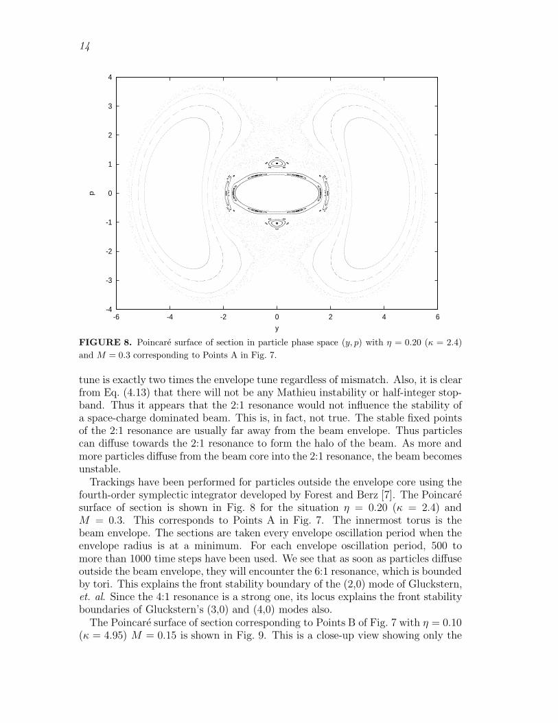
FIGURE 8. Poincare surface of section in particle phase space (y, p) with η = 0.20 (κ = 2.4)and M = 0.3 corresponding to Points A in Fig. 7.

tune is exactly two times the envelope tune regardless of mismatch. Also, it is clearfrom Eq. (4.13) that there will not be any Mathieu instability or half-integer stop-band. Thus it appears that the 2:1 resonance would not influence the stability ofa space-charge dominated beam. This is, in fact, not true. The stable fixed pointsof the 2:1 resonance are usually far away from the beam envelope. Thus particlescan diffuse towards the 2:1 resonance to form the halo of the beam. As more andmore particles diffuse from the beam core into the 2:1 resonance, the beam becomesunstable.

Trackings have been performed for particles outside the envelope core using thefourth-order symplectic integrator developed by Forest and Berz [7]. The Poincaresurface of section is shown in Fig. 8 for the situation η = 0.20 (κ = 2.4) andM = 0.3. This corresponds to Points A in Fig. 7. The innermost torus is thebeam envelope. The sections are taken every envelope oscillation period when theenvelope radius is at a minimum. For each envelope oscillation period, 500 tomore than 1000 time steps have been used. We see that as soon as particles diffuseoutside the beam envelope, they will encounter the 6:1 resonance, which is boundedby tori. This explains the front stability boundary of the (2,0) mode of Gluckstern,et. al. Since the 4:1 resonance is a strong one, its locus explains the front stabilityboundaries of Gluckstern’s (3,0) and (4,0) modes also.

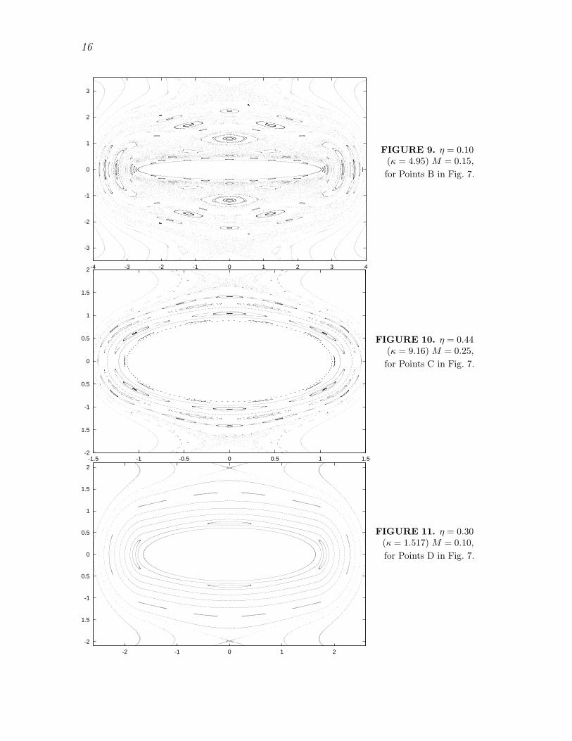
The Poincare surface of section corresponding to Points B of Fig. 7 with η = 0.10(κ = 4.95) M = 0.15 is shown in Fig. 9. This is a close-up view showing only the

15

region near the beam envelope; the 2:1 resonance and its separatrices are not shownbecause they look similar to those depicted in Fig. 8. We see resonances like 14:2,8:1, 16:2, 9:1, 10:1, etc, which are so closely spaced that they overlap to form achaotic region. Particles that diffuse outward from the beam envelope will wandereasily towards the 2:1 resonance along its separatrix. This region, where η <∼ 0.2,is therefore very unstable.

Figure 10 shows the close-up Poincare surface of section of Points C in Fig. 7with η = 0.44 (κ = 0.916) and M = 0.25. Here the particles see many parametricresonances when they are outside the beam envelope; first the 10:3, followed bythe 6:2, 8:3, 10:4, and then a chaotic layer going towards the 2:1 resonance. Theresonances are separated by good tori and the instability growth rate should besmall. Thus, this is the region on the edge of instability.

On the other hand, the Poincare surface of section in Fig. 11 corresponding toPoints D of Fig. 7 with η = 0.30 (κ = 1.517) and M = 0.10 shows the 6:2 resonancewell separated from the 10:4 resonance with a wide area of good tori. Also the widthof the 10:4 resonance is extremely narrow so that particles can hardly be trappedthere. Unlike the situation in Figs. 9 and 10, there is no chaotic region at theunstable fixed points and inner separatrices of the 2:1 resonance, making diffusiontowards this resonance impossible. This region will be relatively stable.

Next let us consider the region with very large beam envelope mismatch likePoints E of Fig. 7 with η = 0.50 (κ = 0.75) and M = 0.60. (The other Point E isat Rmax/R0 = 2.067 and is therefore not visible in Fig. 7). The close-up Poincaresurface of section in Fig. 12 shows the beam envelope radius at y = 0.566 whenpy = 0. We can see that the unstable fixed points and the inner separatrices of2:1 resonance are very close by and are very chaotic. As soon as a particle diffusesout to y = 0.62, it reaches the chaotic sea and wanders towards the 2:1 resonance.Because the chaotic region is so close to the beam envelope, this region of largemismatch is also unstable. As a result, we can interpret Gluckstern’s region ofinstability at large mismatch as chaotic region leading to the 2:1 resonance beingtoo close to the beam envelope.

Finally, we look at Points F of Fig. 7, which have small space charge κ = 0.0106or η = 0.90 and small mismatch M = 0.10. The Poincare surface of sectionis shown in Fig. 13. The beam envelope is surrounded by good tori far awayfrom the separatrices of the 2:1 resonance and no parametric resonances are seen.This is evident also from Fig. 7 that this region is not only free from primaryresonances but also many higher-order resonances. The unstable fixed points andthe separatrices of the 2:1 resonance are well-behaved and not chaotic. Thus thesepoints are very stable. If we keep the same space-charge perveance and increasethe amount of envelope mismatch, we also do not see in the Poincare surface ofsection any parametric resonances between the beam envelope and the separatricesfor the 2:1 resonance. However, although the separatrices of the 2:1 resonanceare not chaotic, they become closer and closer to the beam envelope. When theseparatrices are too close, particles that are driven by a small perturbation awayfrom the beam envelope will have a chance of traveling along the separatrices of

16

-3

-2

-1

0

1

2

3

-4 -3 -2 -1 0 1 2 3 4

FIGURE 9. η = 0.10(κ = 4.95) M = 0.15,for Points B in Fig. 7.

-2

-1.5

-1

-0.5

0

0.5

1

1.5

2

-1.5 -1 -0.5 0 0.5 1 1.5

FIGURE 10. η = 0.44(κ = 9.16) M = 0.25,for Points C in Fig. 7.

-2

-1.5

-1

-0.5

0

0.5

1

1.5

2

-2 -1 0 1 2

FIGURE 11. η = 0.30(κ = 1.517) M = 0.10,for Points D in Fig. 7.

17

-2

-1

0

1

2

-1 -0.5 0 0.5 1

FIGURE 12. η = 0.50(κ = 0.75) M = 0.60,for Points E in Fig. 7.

-2

-1.5

-1

-0.5

0

0.5

1

1.5

2

-1.5 -1 -0.5 0 0.5 1 1.5

FIGURE 13. η = 0.90(κ = 0.1056) M = 0.10,

for Points F in Fig. 7.

the 2:1 resonance to form beam halo. From our discussions above, it is clear thatto avoid instability and halo formation, the beam should have small mismatch andbe in a region that is far away from parametric resonances in the plane of mismatchand tune depression. The best solution for stability is certainly when the beam hassmall mismatch and small space-charge perveance.

The deep fissures of the (2,0) mode near η = 4.7 and 5.3 are probably the resultof encountering the 10:3 and 6:2 parametric resonances. The width of the fissuresshould be related to the width of the resonance islands, which can be computed inthe standard way. In general, a lower-order resonance island, like the 4:1, is muchwider than a higher-order resonance island, like the 6:1.

We tried very hard to examine the region between the 4:1 and 10:3 resonanceswith a moderate amount of mismatch. We found this region very stable unless it isclose to the 10:3 resonance. We could not, however, reproduce the slits that appearin Gluckstern’s (4,0) mode.

18

VI ANGULAR MOMENTUM

Most K-V particles have nonzero angular momentum. When angular momentumis included in the discussion, we first extend the particle Hamiltonian of Eq. (4.15)in Floquet notations to both the x and y transverse planes:

Hp =1

2R2(x2 + y2 + p2

x + p2y) + κ[x2 + y2 − ln (x2+y2)] Θ(x2 + y2 − 1) . (6.1)

It is preferable to use the circular coordinates (r, ϕ) as independent variables; theircanonical momenta are, respectively, pr and pϕ. The particle Hamiltonian becomes

Hp =1

2R2

(r2 + p2

r +p2ϕ

r2

)+ κ(r2 − ln r2) Θ(r − 1) , (6.2)

where r2 = x2 + y2 and pr

pϕr

=

cosϕ sinϕ

− sinϕ cosϕ

px

py

. (6.3)

Extending the generating function in Eq. (4.14) to include the x coordinates, it isstraightforward to show

r = R r and pϕ = xpy − ypx = xpy − ypx . (6.4)

Thus pϕ is the angular momentum of the particle, which is a constant of motion.Since it has the same functional form in both coordinate systems, its overheadaccent ˆ will no longer be necessary. Particles belonging to the unperturbed K-Vdistribution are therefore subjected to the restriction

r2 + p2r +

p2ϕ

r2= 1 , (6.5)

from which we obtain

r2 =1− p2

r

2+

(1− p2r

2

)2

− p2ϕ

1/2

. (6.6)

Thus a K-V particle has an angular momentum restricted by

|pϕ| ≤|1− p2

r|2

≤ 1

2, (6.7)

which agrees with the result of Riabko [6] that 2Jr+ |pϕ| = 12, where Jr is the radial

action. The equation of motion for the particle radial position inside the beam coreis

19

d2r

dψ2+ r −

p2ϕ

r3= 0 , (6.8)

where the Floquet phase advance dψ = dθ/R2 has been used. Notice that this isexactly the same as the envelope equation in Eq (4.10) with κ = 0. We proved inSec. II that the envelope tune is exactly twice the particle tune when κ→ 0. Hence,comparing with the equation of motion of a zero-angular-momentum particle in thepresence of a mismatched space-charge dominated beam, i.e., Eq. (4.13), we canconclude that the particle radial tune inside the beam core is exactly twice thezero-angular-momentum particle tune for any space charge and mismatch.

Simulations have been performed for the time evolution of the radial motionof a beam particle and then compared with the time evolution of the transversemotion of a particle with zero momentum. One of the simulations is shown inthe upper plot of Fig. 14. The particle is a K-V particle with angular momentumpϕ = 0.3 satisfying the K-V restriction of Eq. (6.6) in a mismatched beam envelopewith M = 0.30 having a tune depression of η = 0.23. We see that the shapeof oscillations of r shown as solid is very similar to that of y with zero angularmomentum shown as dashes. Since r does not go negative, its tune appears to betwice the tune of a zero angular-momentum particle. This plot was performed neara 6:1 resonance for a zero angular-momentum particle and it therefore translatesinto a 3:1 resonance for a nonzero angular-momentum particle.

It is interesting to point out that as |pϕ| → 12, the humps that exhibit in the

time evolution of the radial motion become more pronounced and time evolutioneventually becomes proportional to the envelope oscillation, as is demonstratedin lower plot of Fig. 14. Now the radial tune appears to change suddenly to theenvelope tune instead. In fact, this is easy to understand. The equation of motionfor the particle radial position is

r′′ + r =2κ

R2r +

pϕr3

. (6.9)

Comparing with the envelope equation (4.10), it is evident that r =√|pϕ|R is

a solution. Of course, in the Floquet representation, Eq. (6.8) also reflects sucha solution. Thus, we come across an ambiguity that the radial tune can assumetwo different values. This ambiguity can be resolved by investigating the Poincaresurface of section of the radial motion. In the Floquet coordinates, the trajectory

is represented by one point, r =√|pϕ| and pr = 0. In the (r, pr) coordinates,

the Poincare surface of section is also a single point since the phase-space positionof the particle is plotted only every envelope period. In fact, from Eq. (6.2), the

Hamiltonian in the Floquet representation, it is clear that the solution r =√|pϕ|

is the lowest point of the radial potential. This is the equilibrium solution which,in the case of a Hill’s equation, is equivalent to a particle traveling along an orbitpassing through the centers of all elements. Therefore, even in this solution, theradial tune is not equal to the envelope tune, but remains twice the tune in theCartesian coordinates.

20

FIGURE 14. Plots showing the time evolution of the radial position r of a K-V particle insolid with nozero angular momentum inside a beam envelope with mismatch M = 0.30 andspace-charge perveance κ = 2.059 (η = 0.23). The time evolution y of a zero-angular-momentumparticle is also shown in dashes. The simulation has been performed at the 6:1 resonance for thezero-angular-momentum particle. In the top plot, the radial motion has an angular momentumof pϕ = 0.30. The radial oscillation is two times as fast as that of the particle with zero angularmomentum. In the lower plot, the angular momentum has been increased to pϕ = 0.50. Nowthe particle radius r is related to the envelope radius R by r =

√|pϕ|R = R/

√2, giving a false

impression that the radial tune becomes equal to the envelope tune.

21

Because of the above discussion, all the n:m parametric resonances that we stud-ied in Sec. V just translate into the n

2:m resonances in a r-pr Poincare surface of

section. As a result, the stability investigation in the previous section should holdeven when particles with finite angular momentum are included.

VII CONCLUSIONS

(a) Collective instabilities of a K-V beam in a uniformly focusing channel havebeen explained using the particle-beam nonlinear-dynamics approach. First, theloci of the first- and higher-order parametric resonances were mapped in the planeof tune depression and beam envelope mismatch. Different regions in this planewere discussed in terms of their potential for unstable motion. Because the K-Vequation is far from realistic, and because of the existence of noises of all typesin the accelerators (as well as in the numerical simulations), some particles willdiffuse away from the K-V distribution. If the beam envelope ellipse is boundedby invariant tori, and if the diffusion rate is small, the beam will eventually reachequilibrium and we consider this situation stable.

When the particle tune is equal to some fractional multiples of the envelope tune,particle motion encounters parametric resonances in the presence of the space-charge force. As shown in Fig. 6, the resonance strengths for K-V particle arezero inside the beam envelope. However, if the diffusion process is included, theresonance strengths seen by the K-V particles become nonzero and even large assoon as the particles diffuse outside the beam envelope. These particles can movealong the separatrices of the parametric resonances, and eventually escape fromthe K-V core.

As particles escape from the K-V core, density fluctuations will occur in theK-V core. Furthermore, this may enhance the envelope oscillations, driving moreparticles to the outside of the K-V core. Such a process can induce collective beaminstabilities.

It may happen that the island chains outside the beam envelope are so close to-gether that they overlap to form a chaotic sea. In the case where the last invarianttorus breaks up, particles leaking out diffuse towards the 2:1 resonance, which isusually much farther away from the beam envelope. These particles form a beamhalo. As particles escape from the beam envelope, the beam intensity inside the en-velope becomes smaller and the equilibrium radius of the beam core shrinks. Thusmore particles will find themselves outside the envelope radius. As this processcontinues, the beam eventually becomes unstable.

Another severe instability occurs when the envelope mismatch is large eventhough the space-charge perveance is moderate. In this case, high-order para-metric resonances exist near beam envelope. Since the slope of the tune versus theparticle action is small, high-order resonances overlap causing more local chaos.Also the unstable fixed points of the 2:1 resonance are nearby. Particles can diffuseeasily from the beam envelope towards the 2:1 resonance and again become halo

22

particles.

It appears that the particle beam will be most stable when the beam envelopeis far from parametric resonances. Obviously, this occurs when the space-chargeperveance and envelope mismatch are both small.

(b) We see that the regions of stability and instability are similar to but not ex-actly the same as the results of Gluckstern, et. al. There can be many reasons:

1. Only particles outside the envelope core encounter parametric resonances. Sofar we have been using particle tune Qp inside the envelope core. The tuneoutside the core is larger. This may produce more curvature of the resonanceloci in Fig. 7.

2. Gluckstern, et. al. introduced an envelope tune that depends on the space-charge perveance κ only, but is independent of the amount of envelope mis-match. We used an envelope tune that varies with the amount of mismatch.

3. To the lowest order, the Vlasov equation studied by Gluckstern, et. al. doesinvolve the perturbation force induced by the perturbation distribution, f1, orPoisson’s equation of (3.3). In our nonlinear dynamics approach, the particlethat escapes from the beam envelope core, always sees the Coulomb force ofthe entire unperturbed beam core, independent of any variation of the coredistribution due to the leakage of particles. This is a shortcoming in our ap-proach, which we need to improve in the future.

4. Although the results of Gluckstern, et. al. had been checked by simulationsusing a particle-in-cell code, we suspect the simulations do not have sufficientprecision. For example, in one envelope period, the code [8] uses only 100time steps and only first-order symplectic tracking. In our simulations, weused a fourth-order symplectic integrator [7], and found that at least 500 andsometimes more than 1000 time steps are required in many circumstances.Also, the projections of the perturbed distribution onto the various excitationmodes exhibit large fluctuations. Therefore, the growth rates as evaluatedmight not have been accurate.

(c) The reason that the perturbative force induced by the perturbation distribu-tion has not been included in our discussion is mainly due to the fact that we havebeen using the envelope Hamiltonian and the particle Hamiltonian separately. Thisleads to a dependency of the particle equation of motion on the envelope radius,but not the dependency of the equation of motion of the envelope radius on theparticle motion. We believe that this is also the reason why we have not been ableto compute the growth rates of instabilities.

(d) It is possible that many collective instabilities can be explained by the particle-beam nonlinear dynamics approach. The wakefields of the beam interacting withthe particle distribution produce parametric resonances and chaotic regions. Col-lective instabilities will be the result of particles trapped inside these resonanceislands. The perturbed bunch structure further enhances the wakefields to inducethese collective particle instabilities.

23

REFERENCES

1. I.M. Kapchinskij and V.V. Vladimirskij, Proceedings of the International Conf. onHigh Energy Accelerators, p. 274 (CERN, Geneva, 1959).

2. D.D. Caussyn, et. al., Phys. Rev. A46, 7942 (1992); M. Ellison, et. al., Phys. Rev.Lett. 70, 591 (1993); M. Syphers, et. al., Phys. Rev. Lett. 71, 720 (1993); D. li et. al.,Phys. Rev. E48, R1638 (1993); D. li et. al., Phys. Rev. E48, 3 (1993); H. Huanget. al., Phys. Rev. E48, 4678 (1993); Y. Wang et. al., Phys. Rev. E49, 1610 (1994);Y. Wang et. al., Phys. Rev. E49, 5697 (1994); S.Y. Lee et. al., Phys. Rev. E49, 5717(1994); M. Ellison et. al., Phys. Rev. E50, 4051 (1994); L.Y. Liu et. al., Phys. Rev.E50, R3344 (1994); D. Li et. al., Nucl Inst. Methods A 364, 205 (1995).

3. E. Keil and W. Schnell, CERN Report SI/BR/72-5, 1972; D. Boussard, CERN ReportLab II/RF/Int./75-2, 1975.

4. R.L. Gluckstern, W.-H. Cheng, and H. Ye, Phys. Rev. Lett. 75, 2835 (1995);R.L. Gluckstern, W.-H. Cheng, S.S. Kurennoy, and H. Ye, Phys. Rev. E54, 6788(1996).

5. S.Y. Lee and A. Riabko, Phys. Rev. E51, 1609 (1995).6. A. Riabko, M. Ellison, X. Kang, S.Y. Lee, D. Li, J.Y. Liu, X. Pei, and L. Wang, Phys.

Rev. E51, 3529 (1995).7. E. Forest and M. Berz, LBL Report LBL-25609, ESG-46, 1989.8. S.S. Kurennoy, private communication.