Partially Identifying the Impact of the Supplemental ...npc.umich.edu/publications/u/working_paper11-03.pdf · error processes, we ... that are straightforward to motivate in practice

National Poverty Center Working Paper Series

#11 – 03

March 2011

Partially Identifying the Impact of the Supplemental Nutrition

Assistance Program on Food Insecurity among Children:

Addressing Endogeneity and Misreporting Using the SIPP

Craig Gundersen, University of Illinois

Brent Kreider, Iowa State University

John Pepper, University of Virginia

This paper is available online at the National Poverty Center Working Paper Series index at:

http://www.npc.umich.edu/publications/working_papers/

This project was supported by the National Poverty Center (NPC) using funds received from the

U.S. Census Bureau, Housing and Household Economics Statistics Division through contract

number 50YABC266059/TO002. The opinions and conclusions expressed herein are solely those

of the authors and should not be construed as representing the opinions or policy of the NPC or

of any agency of the Federal government.

http://www.npc.umich.edu/publications/working_papers/

Partially Identifying the Impact of the Supplemental Nutrition Assistance Program on Food

Insecurity among Children: Addressing Endogeneity and Misreporting Using the SIPP*

Craig Gundersen Department of Agricultural and Consumer Economics

University of Illinois [email protected]

Brent Kreider

Department of Economics

Iowa State University

[email protected]

John Pepper Department

of Economics University

of Virginia

[email protected]

January 27, 2011

Abstract: Using data from the 2004 panel of the Survey of Income and Program Participation (SIPP),

we reexamine the impact of the Supplemental Nutrition Assistance Program (SNAP) – formerly known as

the Food Stamp Program – on child food insecurity. By far the largest food assistance program in the

United States, SNAP‟s central goal is to alleviate food insecurity. In this light, policymakers have been

perplexed to find positive associations between food insecurity and the receipt of SNAP. Exploiting

recent validation data and detailed information on income and program eligibility in the SIPP, we extend

recent research that confronts the two main issues confounding identification of the causal impacts of

SNAP on food security: endogenous selection into the program and extensive systematic misreporting of

participation status. Imposing relatively weak nonparametric assumptions on the selection and reporting

error processes, we provide tight bounds on the impact of SNAP on child food insecurity. The SIPP is

especially well suited for this project because, along with containing information on food insecurity, it

includes all of the information needed to establish eligibility into the program (other datasets are less

comprehensive), and SNAP participation is observed at repeated intervals over time.

Keywords: Food Stamp Program, Supplemental Nutrition Assistance Program, food insecurity, health outcomes,

partial identification, treatment effect, nonparametric bounds, classification error

* The authors acknowledge financial support from the Survey of Income and Program Participation Analytic

Research Small Grants Competition of the National Poverty Center. Pepper also acknowledges financial support

from the Bankard Fund for Political Economy. The views expressed in this paper are solely those of the authors.

mailto:[email protected]





1

I. Introduction

The literature assessing the efficacy of the Supplemental Nutrition Assistance Program (SNAP),

formerly known as the Food Stamp Program, has long puzzled over positive associations

between SNAP receipt and various undesirable health outcomes such as food insecurity. SNAP

is by far the largest food assistance program in the United States and alleviating food insecurity

is the central goal of SNAP (U.S. Department of Agriculture, 1999). As such, policymakers

expect this program to play an important role in mitigating the incidence of food insecurity.

Paradoxically, however, households receiving SNAP are found much more likely to be food

insecure than observationally similar nonparticipating households. Clearly, important questions

remain about the efficacy of SNAP, and these questions are especially pressing in light of an

unprecedented 30% increase in the food insecurity rate from 2007 to 2008 (Nord et al., 2009).

Using data from the 2004 panel of the Survey of Income and Program Participation

(SIPP), we reexamine the impact of SNAP on child food insecurity. SNAP is thought to play an

especially vital role for children who constitute 60% of all recipients. In any given month, SNAP

provides assistance to more than 15 million children (Wolkwitz and Trippe, 2009), and nearly

half of all children will receive assistance at some point during their childhood (Rank and

Hirschl, 2009). Moreover, policymakers and program administrators have expressed a great deal

of interest in alleviating food insecurity among children. Children in households suffering from

food insecurity are more likely to have poor health, psychosocial problems, frequent

stomachaches and headaches, behavior problems, worse developmental outcomes, more chronic

illnesses, less mental proficiency, and higher levels of iron deficiency with anemia. (See

Gundersen and Kreider, 2009 for an overview of this literature.)

2

Properly evaluating causal impacts of SNAP have proven to be difficult for two central

reasons. First, up to half of all eligible children do not participate in the program, and a

household‟s decision to participate in SNAP is not random. Neglecting this “endogenous

selection problem” confounds researchers‟ and policymakers‟ understanding of SNAP. The

second challenge involves the extensive nonrandom misreporting of SNAP participation status in

surveys, estimated to be as high as 25% in some studies.1

While these identification problems have long been known to confound inferences on the impact of SNAP, credible solutions remain elusive. The literature evaluating the causal impact of

means-tested assistance programs such as SNAP, for example, typically relies on linear response

models coupled with an assumption that some observed instrumental variable (IV), often based

on cross-state and time variation in program rules and regulations, affects program participation

but otherwise has no effect on the outcomes. Yet SNAP is defined at the federal level and has

not substantively changed since the early 1980s, so program rules and regulations are not as

useful as instrumental variables. 2

Moreover, addressing the problem of classification errors is

particularly difficult since the classical model assumption of non-mean-reverting errors cannot

apply with binary variables, and the systematic underreporting of SNAP participation violates

the classical assumption that measurement error arises independently of the true value of the

underlying variable. As a result, little prior research has considered the endogenous selection

1 Using administrative data matched with data from the Survey of Income and Program Participation (SIPP), for

example, Bollinger and David (1997) find that errors in self-reported food stamp recipiency exceed 12 percent and are

related to respondents‟ characteristics including their true participation status, health outcomes, and demographic

attributes. Bitler, Currie, and Scholz (2003) provide similar evidence of extensive underreporting in the Current

Population Survey (CPS).

2 A number of state level policies have been found to be associated with SNAP receipt (see Ratcliffe et al., 2008), but

this policy variation may not be exogenous. That is, states may modify SNAP rules and eligibility criteria in

response to the extent of food insecurity rates. As an example, due to increases in food insecurity, states may reduce

recertification periods to make staying in the program easier for eligible households. This would then lead to an

increase in administrative error rates, one measure that is often used as an instrument in studies of the impact of

SNAP on outcomes.

3

problem, and almost no research has assessed how household reporting errors may affect

inferences about the impacts of the program.3

We reexamine the impacts of SNAP on child insecurity by extending the recently

developed nonparametric statistical methods in Kreider, Pepper, Gundersen, and Jolliffe (2009;

KPGJ hereafter). Using data from the National Health and Nutrition Examination Survey

(NHANES), KPGJ formally address both the endogenous selection and classification error

problems in a single methodological framework by applying partial identification methods that

allow one to consider weaker assumptions than required under conventional parametric

approaches (also see e.g., Manski, 1995; Pepper, 2000; Molinari, 2010; Kreider and Pepper,

2007 and 2008; Gundersen and Kreider, 2008; Kreider and Hill, 2009). These partial

identification methods do not require the linear response model, the classical measurement error

model, or a traditional instrumental variable assumption. Instead, we focus on weaker models

that are straightforward to motivate in practice and result in logically sharp bounds based on the

set of maintained assumptions.

We build on the work in KPGJ in several dimensions. First, we replicate and extend the

earlier work of KPGJ using data from the 2004 panel of the Survey of Income and Program

Participation (SIPP) and, in particular, the Wave 5 Topical Module which includes a series of

food insecurity questions. We also use information on SNAP participation from all eight waves

combined with information needed to establish SNAP eligibility from Waves 3 and 6.

3 There are a few notable exceptions that address the selection problem. Borjas (2004), Gundersen and Oliveira

(2001), Hoynes and Schanzenbach (2009), Meyerhoefer and Pylypchuk (2008), Van Hook and Balistreri (2006) and

Yen et al. (2008) address the selection problem using instrumental variables within a linear response model, and

Devaney and Moffitt (1991) and Ratcliffe and McKernan (2010) use nonlinear selection models. Interestingly,

Devaney and Moffitt (1991) found no significant evidence of selection bias in their consideration of the effect of

food stamps on dietary intakes. Ratcliffe and McKernan (2010), however, estimate that SNAP reduces food

insecurity using the selection model, but not otherwise. The one study that explicitly addresses the classification

error program is Gundersen and Kreider (2008). They formally allow for the possibility of misclassified program

participation, but they focus on identifying descriptive statistics without attempting to identify counterfactual

outcomes.

4

Compared with other datasets, the SIPP data have the advantage of providing much more

accurate and detailed information about income and SNAP eligibility. Second, the panel nature

of the SIPP allows us to incorporate “partial verification” assumptions that reduce the degree of

uncertainty about the reliability of self-reported program participation status. Third, we exploit

recent validation data to narrow the range of uncertainty about SIPP households‟ rates of false

positive and false negative SNAP participation.4

Finally, similar to a regression discontinuity

design, we will introduce into this literature a new way to conceptualize an instrumental variable (IV) assumption using program eligibility as a monotone instrument. There is a long history of

using ineligible respondents to identify the impact of a wide array of public policies. While the

basic idea of the discontinuity design is appealing, in practice considerable disagreement often

arises over the assumption that ineligible respondents reveal the counterfactual outcome

distribution for participants. In contrast, the Monotone Instrumental Variable (MIV) assumption

allows us to relax this traditional identifying assumption by holding that mean outcomes among

subgroups of ineligible respondents bound instead of identify the counterfactual outcome

distribution. The detailed income data in the SIPP is central to operationalizing this assumption.

After describing the data in Section 2, we formally define the empirical questions and

identification problems in Section 3. Following KPGJ, we modify the Manski (1995) selection

bounds to account for classification error in the treatment and we then introduce a number of

assumptions that help tighten inferences.

To account for measurement error, we apply three basic assumptions: first, misreporting

rates cannot exceed 25%; second, there are no false positive errors; and third, households that

report participating in any wave of the SIPP are assumed to provide accurate reports in all waves.

4 Sources of food stamp validation data for the SIPP include Marquis and Moore (1990), Bollinger and David

(1997), Taeuber et al. (2004), and Meyer et al. (2009). We will directly incorporate evidence from these analyses in

the next draft of our paper.

5

These three assumptions are generally consistent with evidence from related validation studies

that find errors of commission to be negligible (0.3%), error rates among households reporting

not to have received food stamps have been found to lie between 10% and 25%, and those who

report SNAP receipt in one period are likely to be accurate reporters in other periods (Bollinger

and David, 2005).

To account for the selection problem, we apply three different types of identifying

assumptions that restrict the relationship between SNAP and food insecurity. First, the

Monotone Treatment Selection (MTS) assumption formalizes the notion of adverse treatment

selection that SNAP recipients are more likely to be food insecure than nonrecipients regardless

of whether they actually would have taken up on the program (Manski and Pepper, 2000).

Second, we consider several variations of the Monotone Instrumental Variable (MIV)

assumption that the latent probability of food insecurity is thought to vary monotonically with

certain observed covariates. As in KPGJ, we will assume this probability decreases with the

income of a child‟s household and, as noted above, we will extend this idea to consider the

identifying power of the discontinuity that arises from income eligibility cutoffs. A central

advantage to SIPP (in comparison to the December Supplement of the CPS and NHANES) is

that income is measured as a continuous rather than as a categorical variable.5

Finally, we

consider the Monotone Treatment Response (MTR) assumption that SNAP cannot lead to an increase in food insecurity (Currie, 2003).

Our empirical results are presented in Section 4, and we draw conclusions in Section 5.

As in KPGJ, we find that under the MIV and MTS assumptions the expansion of SNAP to all

eligible recipients would lead to declines in food insecurity rates. This result, however, does not

hold with modest degrees of misclassification error. Under the joint MIV-MTS-MTR

5 A central goal of SIPP is a more comprehensive and accurate portrayal of income receipt in the U.S.

(http://www.census.gov/sipp/intro.html)

http://www.census.gov/sipp/intro.html)



6

assumption, however, we can conclude that such an expansion would lead to declines in food

insecurity rates even when allowing for high rates of classification error.

II. Data

We use data from the Survey of Income and Program Participation (SIPP). SIPP,

conducted by the U.S. Census Bureau, is a series of national panels designed to measure the

effectiveness of existing government programs such as SNAP and the economic situation of

people in the United States.6

Our research primarily relies on data 2004 SIPP which surveyed

46,500 households eight times over a 2 ½ year period.7

Using data from the wave 5 interview, we focus our analysis on households with children

eligible to receive SNAP. SNAP is available to all households that meet income and asset tests.

To be eligible for assistance, a household‟s gross income before taxes in the previous month

cannot exceed 130 percent of the poverty line, net monthly income cannot exceed the poverty

line, and assets must be less than $2,000. 8

As is done in much of the literature, we examine

children residing in gross income eligible households (e.g., KPGJ).9

In particular, we use information on household structure and income from the Wave 5 Core Module to identify who is

6 Given the wealth of information on program participation and income, SIPP has been used in previous research on

SNAP. Recent work includes, e.g., Bollinger and David, 2001, 2005; Gundersen and Oliveira, 2001; Ribar and

Hamrick, 2003. 7 While the SIPP oversamples low-income households, our analysis is conditioned on income and in particular low- income households. As a result, we do not use the SIPP survey weights. The primary results, however, are not

sensitive to using weights: the basic patterns are identical and the qualitative results do not change when we use the

person specific weights. 8 There are some exceptions to these rules (e.g., households with someone who has a disability need not meet the gross income criterion; households receiving TANF are categorically eligible) but these criteria hold for the vast

majority of households with children. 9 Given our focus on children, however, the gross income tests should not lead to many errors in defining income eligibility. Nearly all gross income-eligible households are also net income-eligible. Using combined data from

1989 to 2004 from the March CPS (which does have information on the returns to assets), Gundersen and Offutt

(2005) find that only seven percent of households with children are asset ineligible but gross income eligible. In

contrast, the asset test could be important for a sample that includes a high proportion of households headed by an

elderly person (Haider et al., 2003).

7

eligible for SNAP based on the gross income criterion and, out of these households, which have

children. In total, 2,936 children reside in income eligible households. The detailed income and

asset information included in the SIPP also allows us also to further restrict the sample to asset

eligible households.10

Of the 2,936 children residing in income eligible households, 283 are asset

ineligible. Thus, our primary sample includes information on 2,653 children who reside in

income and asset eligible households. 11

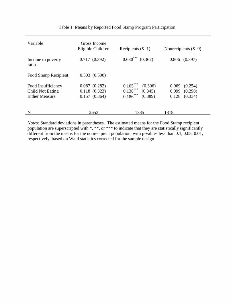
Table 1 displays means and standard deviations for the key variables used in this study. For each respondent, we observe information on household income relative to the poverty line.

Our sample has an average household income level equal to 72 percent of the poverty line, with

respondents claiming to receive SNAP having notably less income than those claiming to have

not received benefits from SNAP.12

We also observe a self-reported measure of SNAP receipt in

the wave five interview (i.e., in the months of February, March, April, and May of 2005) and an

indicator of receipt in any of the eight waves over the 2 ½ year period covered by the 2004

SIPP.13

About half of the eligible households claim to be receiving benefits in wave five, and 66% claim to have received some benefits from SNAP over the 2 ½ years covered by the 2004

SIPP.

10 To determine asset eligibility, we use information from Topical Modules in Waves 3 and 6. Depending on the

state, the value of a vehicle above a certain level may be considered an asset unless it is used for work or for the

transportation of disabled persons. For this paper, however, we do not include the value of respondents‟ vehicles

when defining asset eligibility. 11 Our sample is restricted to Wave 5 respondents. We do use information from other waves for our “ever reported

receiving SNAP” variable. As a consequence, if information from waves are missing and if the respondent does not

report SNAP receipt in any other wave, they receive a value of “0” for “ever reported receiving SNAP”; if respondents do report SNAP receipt in some other wave, they receive a value of “1” for “ever reported receiving

SNAP”. 12 To assess the characteristics of our sample relative to other national estimates, we pool data from six rounds of the 2001-2006 CPS, March Supplement. These data indicate that during this same time period, income eligible children lived in families with average income equal to 70 percent of the poverty line. 13 While a notable proportion of SNAP recipients have imputed values of the amount of benefit receipt, the indicator of receipt is not imputed. Thus, if a household reports receiving SNAP, the value of benefits may be imputed; if it

reports non-receipt, they would not be imputed a positive value of benefits.

8

The participation rate of 50% found in wave five is similar to the contemporaneous rates

found in other surveys (e.g., the CPS and NHAMES) but substantially lower than analogous

rates found when administrative data is used to establish the number of participants. Wolkwitz

(2008) finds, for example, that just over half of all eligible households and eighty percent of

eligible children participate. Differences between the participation rates from administrative and

self-reported surveys are thought to largely reflect classification errors in the self-reported survey

data (Bitler et al., 2003; Trippe, Doyle, and Asher 1992). 14

In fact, Bollinger and David (1997,

Table 2) provide direct evidence of misreporting in the SIPP by comparing individual reports of

food stamp participation status with matched reports from administrative data. They find that

12.0 percent of responses in the 1984 SIPP involve errors of omission while only 0.3 percent

involve errors of commission (see also Marquis and Moore, 1990).

Using data from the wave five topical module, we also observe two measures of food

insecurity. First, the survey has the food insufficiency question that has been included in

numerous surveys since 1977. This question asks respondents to describe their food intake in

terms of the following: Which of these statements best describe the food eaten in your household

in the last month? Respondents have four choices: enough of the kinds of food we want to eat;

enough but not always the kinds of food we want to eat; sometimes not enough to eat; or often

not enough to eat. Those households reporting that they sometimes or often do not get enough to

eat are defined as „„food insufficient.” Second, we include a variable indicating whether the

child is not eating enough. This question is the thirteenth question in the Core Food Security

Module (CFSM) (Nord et al., 2009; Appendix Table A1).

14 These differences might also reflect the time periods used to measure receipt. While administrative participation

rates are often calculated on an annual basis, the rates reported using SIPP are found using self-reports of

participation over a fourth month window. Bollinger and David (1997), however, provide direct evidence of

misreporting in fourth month period used by the SIPP.

9

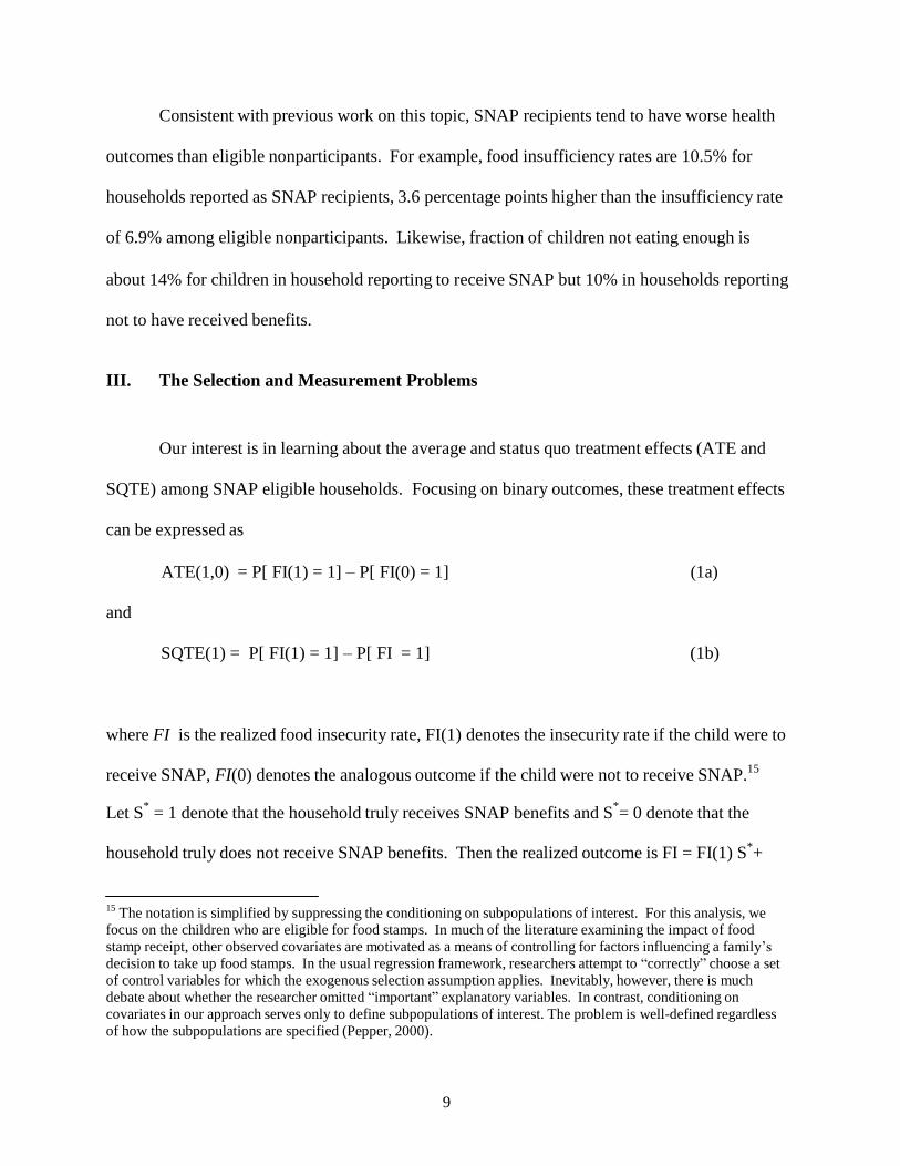
Consistent with previous work on this topic, SNAP recipients tend to have worse health

outcomes than eligible nonparticipants. For example, food insufficiency rates are 10.5% for

households reported as SNAP recipients, 3.6 percentage points higher than the insufficiency rate

of 6.9% among eligible nonparticipants. Likewise, fraction of children not eating enough is

about 14% for children in household reporting to receive SNAP but 10% in households reporting

not to have received benefits.

III. The Selection and Measurement Problems

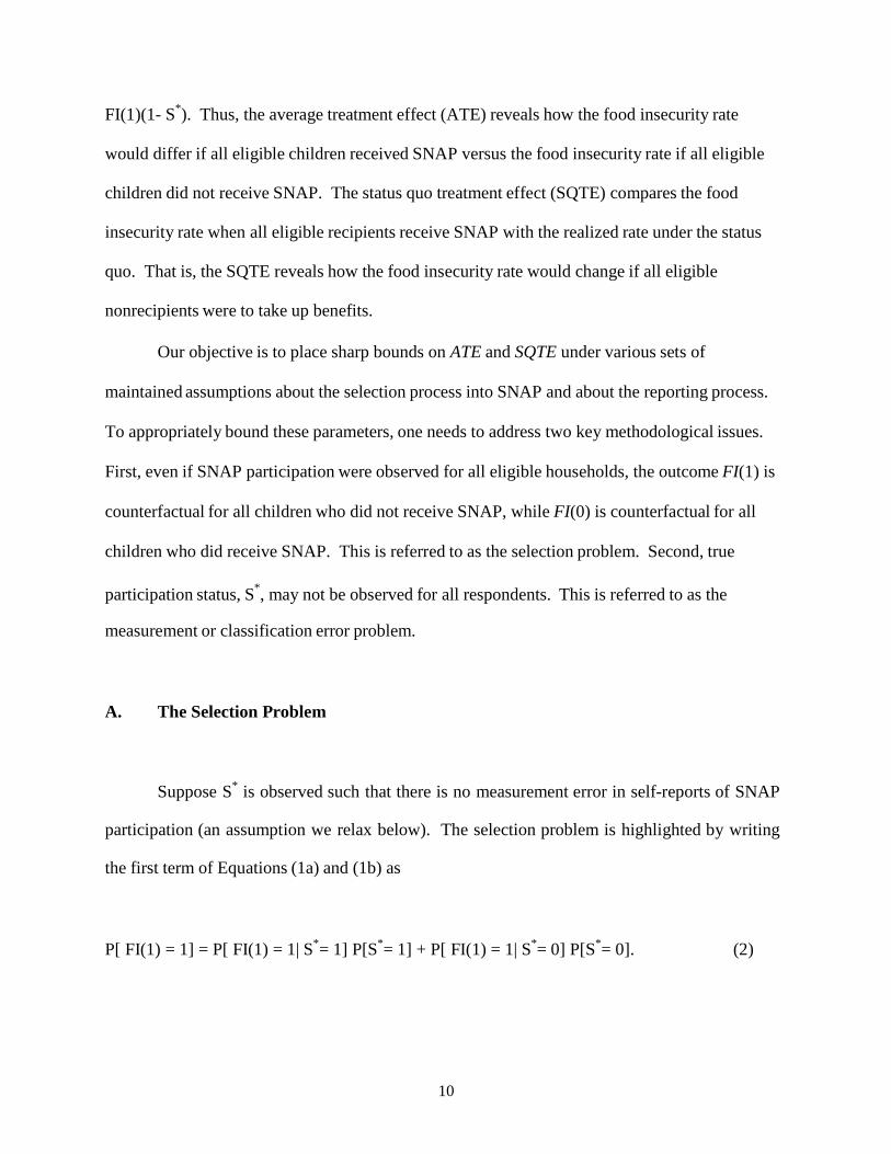
Our interest is in learning about the average and status quo treatment effects (ATE and

SQTE) among SNAP eligible households. Focusing on binary outcomes, these treatment effects

can be expressed as

ATE(1,0) = P[ FI(1) = 1] – P[ FI(0) = 1] (1a)

and

SQTE(1) = P[ FI(1) = 1] – P[ FI = 1] (1b)

where FI is the realized food insecurity rate, FI(1) denotes the insecurity rate if the child were to

receive SNAP, FI(0) denotes the analogous outcome if the child were not to receive SNAP.15

Let S*

= 1 denote that the household truly receives SNAP benefits and S*= 0 denote that the

household truly does not receive SNAP benefits. Then the realized outcome is FI = FI(1) S*+

15 The notation is simplified by suppressing the conditioning on subpopulations of interest. For this analysis, we

focus on the children who are eligible for food stamps. In much of the literature examining the impact of food

stamp receipt, other observed covariates are motivated as a means of controlling for factors influencing a family‟s

decision to take up food stamps. In the usual regression framework, researchers attempt to “correctly” choose a set

of control variables for which the exogenous selection assumption applies. Inevitably, however, there is much

debate about whether the researcher omitted “important” explanatory variables. In contrast, conditioning on

covariates in our approach serves only to define subpopulations of interest. The problem is well-defined regardless

of how the subpopulations are specified (Pepper, 2000).

10

FI(1)(1- S*). Thus, the average treatment effect (ATE) reveals how the food insecurity rate

would differ if all eligible children received SNAP versus the food insecurity rate if all eligible

children did not receive SNAP. The status quo treatment effect (SQTE) compares the food

insecurity rate when all eligible recipients receive SNAP with the realized rate under the status

quo. That is, the SQTE reveals how the food insecurity rate would change if all eligible

nonrecipients were to take up benefits.

Our objective is to place sharp bounds on ATE and SQTE under various sets of

maintained assumptions about the selection process into SNAP and about the reporting process.

To appropriately bound these parameters, one needs to address two key methodological issues.

First, even if SNAP participation were observed for all eligible households, the outcome FI(1) is

counterfactual for all children who did not receive SNAP, while FI(0) is counterfactual for all

children who did receive SNAP. This is referred to as the selection problem. Second, true

participation status, S*, may not be observed for all respondents. This is referred to as the

measurement or classification error problem. A. The Selection Problem

Suppose S*

is observed such that there is no measurement error in self-reports of SNAP

participation (an assumption we relax below). The selection problem is highlighted by writing

the first term of Equations (1a) and (1b) as

P[ FI(1) = 1] = P[ FI(1) = 1| S*= 1] P[S

*= 1] + P[ FI(1) = 1| S

*= 0] P[S

*= 0]. (2)

11

The sampling process identifies the selection probability, P(FS * = 1) , the censoring probability

P(FS * = 0), and the expectation of outcomes conditional on the outcome being observed, P[ FI(1)

= 1| S*= 1]. Still, the sampling process cannot reveal the mean outcome conditional on

censoring, P[ FI(1) = 1| S*= 0]. Given this censoring, P[ FI(1) = 1] is not point-identified by the

sampling process alone. Analogously, the second term in Equation (1a), P[ FI(1) = 1], is not

identified.

Since the latent probability P[ FI(1) = 1| S*= 0] must lie within [0,1], it follows that

P[ FI=1, S* = 1] ≤ P[ FI(1) = 1] ≤ P[ FI=1, S* = 1] + P[ S* = 0] (3)

Intuitively, the width of this bound equals the censoring probability, P[ S* = 0]. Thus, if a large

fraction of children receive SNAP, the width of the bound on is relatively narrow. In that case,

the data cannot reveal much information about the distribution of FI(0), so the analogous bound

of the quantity P[ FI(0) = 1]is larger. Taking the difference between the upper bound on P[ FI(1)

= 1] and the lower bound on P[ FI(0) = 1] obtains a sharp upper bound on ATE, and analogously

a sharp lower bound (Manski, 1995). As a result, the width of the bound on the average

treatment effect always equals 1. In the absence of identifying restrictions, the data cannot reveal

the sign of the effect of SNAP on health outcomes.

B. The Classification Error Problem

To highlight this measurement problem, let the latent variable Z*

indicate whether a

report is accurate, where Z*

=1 if S*= S and Z

*= 0 otherwise. Using this variable, we can further

decompose the first term of Equations (1a) and (1b) as

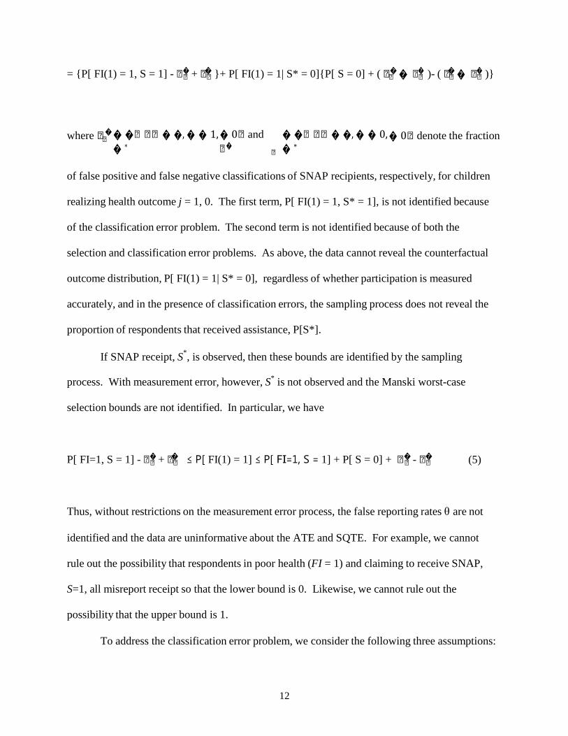
P[ FI(1) = 1] (4) = P[ FI(1) = 1, S* = 1]+ P[ FI(1) = 1| S* = 0]P[ S* = 0]

12

= {P[ FI(1) = 1, S = 1] - � + � }+ P[ FI(1) = 1| S* = 0]{P[ S = 0] + ( � � � )- ( � � � )}

where � � � � �, � � 1, � 0 and � � � �, � � 0, � 0 denote the fraction

� ∗ � � ∗

of false positive and false negative classifications of SNAP recipients, respectively, for children

realizing health outcome j = 1, 0. The first term, P[ FI(1) = 1, S* = 1], is not identified because

of the classification error problem. The second term is not identified because of both the

selection and classification error problems. As above, the data cannot reveal the counterfactual

outcome distribution, P[ FI(1) = 1| S* = 0], regardless of whether participation is measured

accurately, and in the presence of classification errors, the sampling process does not reveal the

proportion of respondents that received assistance, P[S*].

If SNAP receipt, S*, is observed, then these bounds are identified by the sampling

process. With measurement error, however, S*

is not observed and the Manski worst-case

selection bounds are not identified. In particular, we have

P[ FI=1, S = 1] - � + � ≤ P[ FI(1) = 1] ≤ P[ FI=1, S = 1] + P[ S = 0] + � - �

(5)

Thus, without restrictions on the measurement error process, the false reporting rates θ are not

identified and the data are uninformative about the ATE and SQTE. For example, we cannot

rule out the possibility that respondents in poor health (FI = 1) and claiming to receive SNAP,

S=1, all misreport receipt so that the lower bound is 0. Likewise, we cannot rule out the

possibility that the upper bound is 1.

To address the classification error problem, we consider the following three assumptions:

13

(A1) Upper Bound Error Rate Assumption: P(Z*

= 0) ≤ Qu

(A2) No False Positives Assumption: If S = 1, then S*

= S= 1

(A3) Verification Assumption: If V = 1, then S* = S

where Qu places a known upper bound on the degree of data corruption and V indicates if the

respondent reported receiving SNAP in any wave of the 2004 SIPP. Thus, Assumption (A1)

bounds the classification error rate. The literature evaluating the causal impacts of SNAP has

uniformly maintained the assumption of accurate reporting, in which case Qu is implicitly

assumed to be zero. At the opposite extreme, Qu can be set equal to 1 if nothing is known about

the reliability of the participation responses. As noted above, validation studies find false

negative error rates to lie between 10% and 25%. These studies also that find errors of

commission are negligible (Bollinger and David, 1997). Thus, Assumption (A2) rules out false

positive reports; respondents reporting to have received SNAP are known provide accurate

reports.

Finally, panel data from the SIPP allows us to “verify” the receipt of SNAP for some

respondents based on the reporting patterns over time. Bollinger and David (2005), examining

data from the 1984 SIPP, find that respondents who accurately report SIPP participation in one

period are more likely to accurately report in other periods. Moreover, self-reports of receipt are

generally thought to be accurate, as indicated by A2. Thus, under Assumption (A3), we “verify”

that a respondent is an accurate reporter in wave 5 (of receipt or nonreceipt) if, in at least one

wave she reported receiving SNAP.16

In our sample, 66 percent of SNAP eligible households

with children report receiving SNAP in at least one of wave of the 2004 SIPP, whereas 50.3% of

16 A logical extension would be to validate responses using other welfare programs. So, for example, a response of

food stamp receipt can be validated if the respondent reported receiving any welfare program benefits during any

wave of the survey (not just SNAP). In principle, TANF and SSI receipt would be especially relevant as both confer

categorical eligibility for SNAP.

14

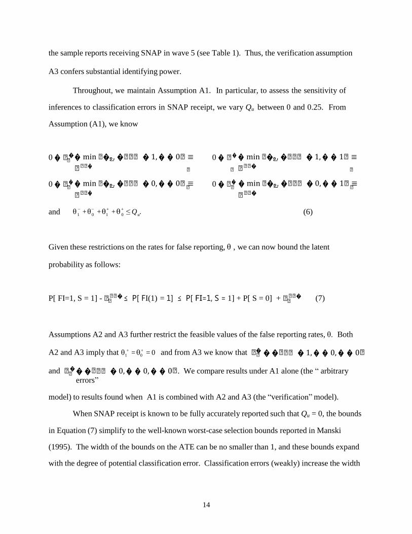
the sample reports receiving SNAP in wave 5 (see Table 1). Thus, the verification assumption

A3 confers substantial identifying power.

Throughout, we maintain Assumption A1. In particular, to assess the sensitivity of

inferences to classification errors in SNAP receipt, we vary Qu between 0 and 0.25. From

Assumption (A1), we know

0 � � � min �௨, � � 1, � � 0 ≡ 0 � � � min �௨, � � 1, � � 1 ≡

� �

� � min �௨, � � 0, � � 0 ≡

0 � � � min �௨, � � 0, � � 1 ≡

0 �

� �

and θ − + θ−

+ θ + + θ +

≤ Q . (6) 1 0 1 0 u

Given these restrictions on the rates for false reporting, θ , we can now bound the latent probability as follows:

P[ FI=1, S = 1] - � ≤ P[ FI(1) = 1] ≤ P[ FI=1, S = 1] + P[ S = 0] + �

(7)

Assumptions A2 and A3 further restrict the feasible values of the false reporting rates, θ. Both

A2 and A3 imply that θ + = θ + = 0 and from A3 we know that � � � � 1, � � 0, � � 0

1 0

and � � � � 0, � � 0, � � 0. We compare results under A1 alone (the “ arbitrary

errors”

model) to results found when A1 is combined with A2 and A3 (the “verification” model).

When SNAP receipt is known to be fully accurately reported such that Qu = 0, the bounds

in Equation (7) simplify to the well-known worst-case selection bounds reported in Manski

(1995). The width of the bounds on the ATE can be no smaller than 1, and these bounds expand

with the degree of potential classification error. Classification errors (weakly) increase the width

15

1 0

of the bounds.17

Without stronger assumptions on the selection process, the data cannot identify

whether participation in SNAP increases or decreases the prevalence of food insecurity.

C. Middle Ground Selection Models

To derive useful inferences about the impact of SNAP on health, prior information on the

selection process must be brought to bear. While the exogenous selection assumption

maintained in much of the literature is untenable, there are a number of middle ground

assumptions that can narrow the bounds by restricting the relationship between SNAP

participation, health outcomes, and observed covariates. We consider the identifying power of

three monotonicity assumptions: one on treatment selection, one on an instrument, and one on

treatment response.

The Monotone Treatment Selection (MTS) assumption (Manski and Pepper, 2000) places

structure on the selection mechanism through which children become SNAP recipients. The

literature suggests that unobserved factors associated with poor health are likely to be positively

associated with the decision to take up the program. In this case, recipients have worse latent

health outcomes than nonrecipients on average.18

We formalize the MTS assumption as follows:

(A4) P[ FI(1) = 1| S* = 0]≤ P[ FI(1) = 1| S* = 1] and

P[ FI(0) = 1| S* = 0]≤ P[ FI(0) = 1| S* = 1].

17 Interestingly, under the A2 assumption of no false positive reports where θ UB , + = θ UB , + = 0 , the bounds on

P[FI(1) =1] in Equation (7) are also identical to the Manski bounds, regardless of the value of Qu. In this case, the

latent SNAP receipt probability cannot be less than the reported probability, P(S=1), and likewise, the latent outcome probability under full participation cannot be less than the observed joint probability of having poor health and receiving SNAP benefits, P(FI=1, S = 1). 18 For information on differences between food stamp recipients and nonrecipients over commonly observed

covariates, see Cunnyngham (2005). For speculation about differences over unobserved characteristics, see, e.g.,

Gundersen and Oliveira (2001) and Currie (2003).

16

మ

That is, conditional on either treatment t = 1 or 0, eligible households that receive SNAP, S*=1,

tend to have a higher prevalence of food insecurity than eligible households that have not taken

up SNAP, S*

= 0.

The Monotone Instrumental Variable (MIV) assumption (Manski and Pepper, 2000) formalizes the notion that the latent probability of a negative health outcome, P[ FI(t) = 1] varies

monotonically with certain observed covariates. Arguably, for example, this probability decreases

with the poverty income ratio (PIR), the ratio of a family's income to the poverty threshold set by

the U.S. Census Bureau accounting for the family's composition.19

To formalize this idea, let v be

the monotone instrumental variable such that

(A5) u1 = u ≤ u2 implies P[ FI(t) = 1 | v = u2 ] ≤ P[ FI(t) = 1 | v = u ] ≤ P[ FI(t) = 1 | v = u1 ]

for t = 0,1.

While these conditional probabilities are not identified, they can be. Let LB(u) and UB(u) be

the known lower and upper bounds evaluated at v = u, respectively, given the available

information. Then the MIV assumption formalized in Manski and Pepper (2000, Proposition 1)

implies:

supஸ ଶ � � � 1 | � � infஹభ � .

19 Table 3 of Nord et al. (2009) demonstrates that food insecurity rates in the U.S. fall as income increases: 50.3%

for those under the poverty line, 46.3% for those under 130% of the poverty line, and 42.2% for those under 185%

of the poverty line versus 10.1% for those over 185% of the poverty line.

17

In the absence of other information, these bounds on P[FI(t) = 1| v = u ] is sharp. Bounds on the

unconditional latent probability, P[ FI(t) = 1 ] can then be obtained using the law of total

probability.20

In addition to using income relative to the poverty line as an MIV, we also formalize the

notion that eligibility criteria for SNAP might be monotonically related to the latent outcomes.

For example, income ineligible children – i.e., children residing in households with income

greater than 130% of the federal poverty line – are likely to have better average health outcomes

the income eligible children. Many program evaluations rely on ineligible respondents to reveal

the counterfactual outcome distribution under nonparticipation. This, for example, is the central

idea of the regression discontinuity design.21

In our application, we observe two groups of ineligible respondents: income eligible

children who fail the asset test (v2 ≡ assets ineligible and children whose household income is

between 130% and 150% of the poverty line (v3 ≡ income ineligible). While these comparison

groups are unlikely to satisfy the standard instrumental variable restriction that the latent food

insecurity outcomes are mean independent of eligibility status, the MIV assumption holding that

mean response varies monotonically across these subgroups seems credible. Children in

households with assets or incomes above the eligibility cutoff for (i.e., above 130% of the

poverty line), are likely to have no worse average latent health outcomes than children living in

eligible households. That is, max{ P[ FI(t) = 1 | v2 = 1] , P[ FI(t) = 1 | v3= 1]} ≤ P[ FI(t) = 1 ].

Moreover, for these ineligible subgroups where v2 = 1 or v3= 1, there is no selection or

classification error problem; we assume S*

= 0.22

The sampling process identifies P[FI(0) = 1|

20 To find the MIV bounds on the rates of poor health, one takes the appropriate weighted average of the plug-in

estimators of lower and upper bounds across 26 PIR groups (more than 100 households per cell) observed in the

data. As discussed in Manski and Pepper (2000), this MIV estimator is consistent but biased in finite samples. We

employ Kreider and Pepper‟s (2007) modified MIV estimator that accounts for the finite sample bias using a

nonparametric bootstrap correction method. 21 For example, Schanzenbach (2007) and Bhattacharya et al. (2006) use ineligible children to identify the impact of school meal programs on health 22 The assumption that S*= 0 (similar to a sharp discontinuity design) may not be valid for the observed income

18

v2=1] and P[FI(0) = 1| v3=1] but provide no information on P[ FI(1) = 1]. Thus, this MIV

restriction implies that max{ P[ FI = 1 | v2 = 1] , P[ FI = 1 | v3= 1]} ≤ P[ FI(0) = 1 ].

Finally, the Monotone Treatment Response (MTR) assumption (Manski, 1997)

formalizes the common idea that SNAP cannot lead to a reduction in health status. Despite the

observed correlations in the data, there is a general consensus among policymakers and

researchers that the SNAP program cannot increase the rate of food insecurity (Currie, 2003).

That is,

(A6) FI(1) ≤ FI(0).

While widely accepted, this the assumption alone signs the effect of the SNAP program on food

insecurity. Under the MTR assumption, the ATE and SQTE of receiving SNAP must be

nonpositive (Manski, 1997 and Pepper, 2000). To assess the sensitivity of inferences to this

MTR restriction, we consider this assumption separately from the MTS and MIV assumptions.

The population bounds derived in this section account only for identification uncertainty

and abstract away from the additional layer of uncertainty associated with sampling variability.

These bounds will be estimated by replacing population probabilities with the corresponding

sample probabilities. Confidence intervals that cover the true value of ATE or SQTE with 95%

probability will be constructed using methods provided by Imbens and Manski (2004).

threshold where income measures used to determine eligibility may reflect different time periods than measures collected in the SIPP. A household whose eligibility was established in one period may have income that exceeds

the threshold when the survey is conducted. With a “fuzzy” threshold where S* = 1 for some “ineligible” respondents, the methods can be adapted to allow for selection and measurement error within “ineligible” subgroups. In this case, the data would provide informative bounds on both latent outcome probabilities.

19

IV. Results

The analytical approach allows us to trace out sharp bounds on ATE and SQTE under

different assumptions about the selection and measurement error problems. To do this, we

evaluate the bounds as a function of the degree of uncertainty about the extent of SNAP

reporting errors and layer on different types of restrictions aimed at addressing the selection

problem.

We begin by considering the traditional case where selection into SNAP participation is

exogenous. That is, P[ FS(t) | S* ] = P[FS(t)]. Under this assumption, the ATE is given by

∆ = P[FS = 1|S* = 1] – P[FS =1 | S* = 0],

the difference in the probability of being food insecure between children receiving and not

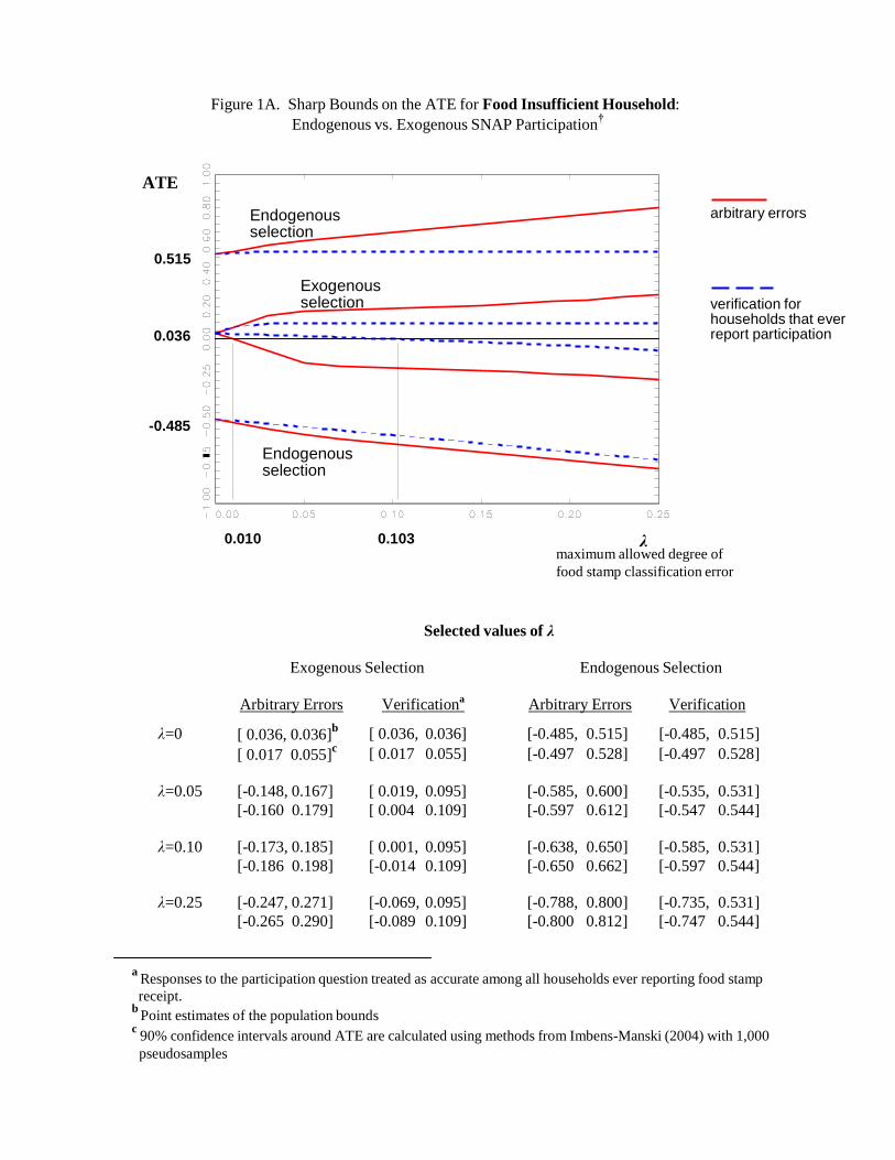
receiving SNAP. Figure 1 traces out sharp bounds on Δ as Qu varies between 0 and 0.25;

throughout, we allow for the possibility that all reports of SNAP receipt are accurate. These

bounds on ∆ are calculated using methods in Kreider and Pepper (2007) for the case of arbitrary

errors (with only A1 imposed) and in Kreider and Hill (2009) for the verification case (with both

A1 and A3 imposed). The associated table displays bounds for the selected values Qu = {0, 0.05,

0.10, 0.25} along with Imbens-Manski (2004) confidence intervals that cover the true value of Δ with 95% probability.

If all SNAP participation responses are known to be accurate (Qu = 0), then Δ is point-

identified in Figure 1 as 0.105-0.069 = 0.036 > 0 (consistent with the descriptive statistics in

Table 1). This difference in children‟s food insufficiency rates between recipients and

nonrecipients is statistically significant with a p-value less than 0.01. When Qu > 0, the food

insufficiency gap can only be partially identified. When an arbitrary 5 percent of households

20

may misreport FS, for example, Δ can lie anywhere in the range [-0.148, 0.167], with the 95

percent confidence interval of [-0.160, 0.179]. These ranges narrow to [0.019, 0.095] and

[0.004, 0.109], respectively, under the verification assumptions A2 and A3.

The key result in Figure 1 is that identification of Δ deteriorates with Qu sufficiently

rapidly, even under the verification assumptions, that we cannot identify that the food insecurity

gap is positive if more than 10 percent of households may have misreported FS. Thus, even

assuming exogenous selection and ignoring the uncertainty associated with sampling variability,

small levels of reporting error imply that the sign of ATE is not identified. Therefore, a

conclusion that food insecurity is more prevalent among SNAP recipients than among eligible

nonrecipients requires a some confidence in self-reported food participation status, an assumption

not supported by validation studies. Similar findings have been reported using data from the CPS

(see Gundersen and Kreider, 2008) and the NHAMES (see KPGJ, 2009).

Figure 1 also displays estimates of the bounds on ATE when we relax the exogenous

selection assumption. If no assumptions are made about how eligible households select

themselves into SNAP receipt and the SNAP participation indicator is presumed to be fully

accurately reported (Qu = 0), the bounds simplify to the well-known Manski (1995) selection

bounds reported in Equation (3). These wide bounds reveal the inherent ambiguity created by

the selection problem. The width of the ATE bounds equals 1, the width of the SQTE bounds

equals P(S=0) = 0.497, and both treatment effect bounds always include zero.

Potential classification errors increase uncertainty about the ATE. When Qu rises from 0

to 0.10, for example, the ATE bounds under the verification assumptions expand from [-0.485,

0.515] with a width of 1 to [-0.535, 0.531] with a width of 1.066. Interestingly, however, the

SQTE bounds are not sensitive to classification errors under the verification model assumptions

21

A2 and A3. This follows from the fact the outcome probability under full take-up, P[FI(1) = 1],

does not vary with Qu and thus the bounds on the SQTE will not either. Regardless of the value

of Qu, SQTE is estimated to lie within the range [-0.034, 0.462] (see Appendix Table A1).

Importantly, this result does not imply that the SQTE is more likely to be positive than negative.

Rather, we learn that effect of expanding SNAP to all eligible households must lie within these

bounds. That is, without imposing any assumptions on the selection problem, we learn that

SNAP may to lead sharp increase in food insufficiency, it may have no impact at all, or it may

lead to a modest decrease. Below, under stronger restrictions on the selection problem, we find

evidence that the SQTE is, in fact, negative.

These wide bounds highlight a researcher‟s inability to make strong inferences about the

efficacy of SNAP without making assumptions that address the problem of unknown

counterfactuals. In the absence of restrictions that address the selection problem, we cannot rule

out the possibility that SNAP has a large positive or negative impact on the likelihood of poor

health. These bounds can be narrowed substantially, however, under common monotonicity

assumptions on treatment response, treatment selection, and the relationship between the latent

outcome and observed instrumental variables.

To narrow the bounds, we first combine the MIV assumptions with the MTS assumption.

The results are displayed in Figures 2A and 2B, and Table 2.23

The most striking finding is that

the joint MIV-MTS model identifies the ATE and SQTE as strictly negative and substantial as

long as the degree of misreporting is small. If participation is accurately reported, Qu = 0, for

example, the bounds on the ATE are estimated to be [-0.402, -0.040] and the SQTE is nearly

23 In Appendix A, we include figures and tables which trace out the bounds using each of these assumptions – the

MIV and MTS – separately. While these bounds are notably narrower than the no assumption bounds in Figure 1,

the assumptions imposed separately do not identify the ATE in this application. Only when we combine the MIV

and MTS assumptions, do we estimate bounds that reveal the sign of the treatment effect.

22

identified, with the estimated bounds of [-0.014, -0.007] (see Table 2). Thus, if participation is

accurately reported, these estimates for the ATE suggest that SNAP reduces food insufficiency

by at least 4 points and the prevalence of not eating enough by at least 7.2 points.24

Likewise,

the estimated SQTE implies that expanding SNAP to all eligible households would reduce the

prevalence of food insufficiency by about a percentage point, or about 10% relative to the status

quo rate of 0.087.

While these findings seem to indicate that the SNAP plays an important role in reducing

food insufficiency, identification of the sign of the ATE is precluded under even small degrees of

classification error. Figure 2 shows that we can only identify ATE < 0 as long as SNAP

misreporting is confined to no more than about 2% of households (under both arbitrary errors

and no false positive errors). Moreover, even with fully accurate reporting, the 90 percent

confidence intervals include zero. Thus, we cannot reject the hypothesis that the program is

ineffective in promoting food sufficiency. Still, while these findings do not clearly identify the

sign of the ATE, the ambiguity created by the selection and measurement problems is notably

reduced under this joint MIV-MTS model. Under low rates of misreporting, SNAP appears to

have at worst negligible impacts on food insecurity and at best may substantially reduce the

prevalence of negative health outcomes.

Finally, under the joint MTR-MTS-MIV assumption, Figure 3 and Table 2 reveal that the

ATE and SQTE can be identified as strictly negative even for large degrees of arbitrary SNAP

misreporting. Under this joint assumption, our estimated bounds for ATE on food insufficiency

rates vary from [-0.402, -0.083] when Qu = 0 to [-0.75, -0.083] when Qu = 0.25. Thus, under this

24 These estimates imply that SNAP leads to substantial reductions in food insecurity. Consider, for example, the

household food insufficiency rate where the estimated bound on the ATE of -0.04 (see Figure 2A) is found by

differencing the estimated upper bound on P[FI(1)=1] of 0.081 and the lower bound on P[FI(0)=1] of 0.121. Thus,

the estimates imply SNAP reduces the prevalence of childhood food insufficiency by at least one third, from 0.12 to

0.08. Likewise, SNAP is estimated to reduce the prevalence of not eating enough by at least -0.07 points, from

0.158 to 0.086, or 46%.

23

model, we find that SNAP reduces the food insufficiency rate by at least 8 percentage points and

perhaps much more. Similar results are found for the prevalence of children not eating enough.

Interestingly, for the SQTE on the food insufficiency rate, the estimated lower bound

often just exceeds the estimated upper bound suggesting that the parameter is point identified.25

In particular, when Qu = 0 under the arbitrary error model and for all Qu in the verification model, the SQTE is estimated to be about -0.02. When the rate of possible misreporting

increases from 0 to 0.25 under the arbitrary error model, the lower bound decreases to -0.087.

Thus, these estimated SQTE bounds imply that expanding SNAP to all eligible households

would reduce the prevalence of food insufficiency by at least two percentage points, or 25%

relative to the status quo rate of 0.08, and perhaps much more.

V. Conclusion

The literature assessing the efficacy of SNAP has long puzzled over positive associations

between SNAP receipt and various undesirable health-related outcomes such as food insecurity.

These associations are often ascribed to the self-selection of more vulnerable households into

SNAP. Misreporting of SNAP recipiency also confounds identification of the causal impacts of

participation on health status. In this paper, we reconsidered the impact of SNAP on food

insecurity using a single unifying framework that formally accounts for both of these

identification problems. Our partial identification approach is well-suited for this application

where conventional assumptions strong enough to point-identify the causal impacts are not

25 There are two reasons the lower bound exceeds the upper bound: first, the underlying model may be invalid and

second, sampling variability. In this application, the bounds do cross but are nearly equal and confidence intervals

do not cross. We take this as evidence that the model is not violated and that the crossing reflects sampling

variability.

24

necessarily credible and there remains much uncertainty about even the qualitative impacts of

SNAP.

Using data from the 2004 SIPP, we make transparent how assumptions on the selection

and reporting error processes shape inferences about the causal impacts of SNAP recipiency on

food insecurity. The potentially troubling correlations in the data provide a misleading picture of

the impacts of SNAP. Without assumptions aimed to address the selection and measurement

problems, the sampling process cannot identify the sign of the effect of SNAP on heath. The

worst-case selection bounds always include zero, and even small amounts of measurement error

are sufficient to cast doubt on the conclusion that food insecurity and other poor health outcomes

are more prevalent among SNAP recipients than among eligible nonrecipients.

Combining the MTS and MIV assumptions, however, allows us sign the impact of SNAP.

Under this relatively weak nonparametric model used to address the selection problem, we find

that SNAP reduces the prevalence of food insufficiency. In the absence of measurement error,

the joint MTS-MIV model reveals that households would be at least 4 percentage points more

likely to be food sufficient if all eligible households received SNAP vs. all not receiving them.

When some households may misreport participation status, however, there remains uncertainty

about the efficacy of the program. Under the joint MTR-MTS-MIV assumption, the basic

conclusion that SNAP reduces the prevalence of food insecurity holds even for large degrees of

measurement error. In this case, we find that households would be at least 8 percentage points

more likely to be food sufficient if all eligible households received SNAP vs. not receiving them

when up to a quarter of households may misreport.

25

References Bhattacharya, J., J. Currie, and S. Haider. 2006. “Breakfast of Champions? The School Breakfast

Program and the Nutrition of Children and Families.” Journal of Human Resources,

41:445-466.

Bitler, M., J. Currie, and J. Scholz. 2003. “WIC Eligibility and Participation.” Journal of Human

Resources, 38: 1139-1179.

Bollinger, C. and M. David. 1997. “Modeling Discrete Choice with Response Error: Food Stamp

Participation.” Journal of the American Statistical Association, 92 (439): 827-835.

Bollinger, C. and M. David. 2001. “Estimation with Response Error and Nonresponse: Food

Stamp Participation in the SIPP.” Journal of Business and Economic Statistics, 19(2):

129-141.

Bollinger, C. and M. David. 2005. “I Didn‟t Tall, and I Won‟t Tell: Dynamic Response Error in

the SIPP.” Journal of Applied Econometrics, 20: 563-569.

Borjas, G. 2004. “Food Insecurity and Public Assistance.” Journal of Public Economics,

88:1421-1443.

Cunnyngham, K. 2005. Food Stamp Program Participation Rates: 2003. Washington, D.C.: U.S.

Department of Agriculture, Food, and Nutrition Service.

Currie, J. 2003. “U.S. Food and Nutrition Programs,” in Means Tested Transfer Programs in the

U.S., ed. Robert Moffitt, University of Chicago Press, Chapter 4.

DePolt R, R. Moffitt , and D. Ribar. 2009. “Food Stamps, Temporary Assistance for Needy

Families and Food Hardships in Three American cities.” Pacific Economic Review,

14(4): 445-473.

Devaney, B., and R. Moffitt. 1991. “Dietary Effects of the Food Stamp Program.” American

Journal of Agricultural Economics, 73(1): 202-211.

Gundersen, C. and B. Kreider. 2009. “Bounding the Effects of Food Insecurity on Children's

Health Outcomes.” Journal of Health Economics, 28:971–983.

Gundersen, C. and B. Kreider. 2008. “Food Stamps and Food Insecurity: What Can Be Learned

in the Presence of Nonclassical Measurement Error?” Journal of Human Resources,

43(2): 352-382.

Gundersen, C. and S. Offutt. 2005. “Farm Poverty and Safety Nets.” American Journal of

Agricultural Economics, 87(4): 885–899.

26

Gundersen, C. and V. Oliveira. 2001. “The Food Stamp Program and Food Insufficiency.”

American Journal of Agricultural Economics, 84(3): 875-887.

Haider, S., A. Jacknowitz, and R. Schoeni. 2003. “Food Stamps and the Elderly: Why is

Participation So Low?” Journal of Human Resources, 38(S): 1080-1111.

Hoynes, H. and D. Schanzenbach. 2009. “Consumption Responses to In-Kind Transfers:

Evidence from the Introduction of the Food Stamp Program.” American Economic

Journal: Applied Economics, 1(4): 109-139.

Imbens, G. and C. Manski. 2004. “Confidence Intervals for Partially Identified Parameters.”

Econometrica, 72(6): 1845-1857.

Kreider, B. and S. Hill. 2009. “Partially Identifying Treatment Effects with an Application to

Covering the Uninsured.” Journal of Human Resources, 44(2): 409-449.

Kreider, B. and J. Pepper. 2007. “Disability and Employment: Reevaluating the Evidence in

Light of Reporting Errors.” Journal of the American Statistical Association, 102(478):

432-441.

Kreider, B. and J. Pepper. 2008. “Inferring Disability Status from Corrupt Data.” Journal of

Applied Econometrics, 23(3): 329-49.

Kreider, B., J. Pepper, C. Gundersen, and D. Jolliffe, 2009. Identifying the Effects of Food

Stamps on Child Health Outcomes. Working Paper.

Manski, C. 1995. Identification Problems in the Social Sciences. Cambridge, MA: Harvard

University Press.

Manski, C. 1997. “Monotone Treatment Response.” Econometrica, 65(6): 1311-1334.

Manski, C. and J. Pepper. 2000. “Monotone Instrumental Variables: With an Application to the

Returns to Schooling.” Econometrica, 68(4): 997-1010.

Marquis, K. and J. Moore. 1990. “Measurement Errors in SIPP Program Reports” in Proceedings

of the Bureau of the Census Annual Research Conference, Wash., DC: Bureau of the

Census, 721-745.

Meyer, B. D., W. K. C. Mock and J. X. Sullivan. 2009. “The Under-Reporting of Transfers in

Household Surveys: Its Nature and Consequences.” NBER Working Paper no. 15181.

Meyerhoefer, C. and V. Pylypchuk. 2008. “Does Participation in the Food Stamp Program

Increase the Prevalence of Obesity and Health Care Spending?” American Journal of

Agricultural Economics, 90(2): 287-305.

27

Molinari, F. 2010.“Missing Treatments.”Journal of Business and Economic Statistics, 28(1):82-

95.

Nord, M., M. Andrews and S. Carlson. 2009. Household Food Security in the United States,

2008. Washington, DC: U.S. Department of Agriculture, Economic Research Report 83.

Pepper, J. 2000. “The Intergenerational Transmission of Welfare Receipt: A Nonparametric

Bounds Analysis.” The Review of Economics and Statistics, 82(3): 472-488.

Rank, Mark R. and Thomas A. Hirschl. 2009. “Estimating the Risk of Food Stamp Use and

Impoverishment During Childhood.” Archives of Pediatrics and Adolescent Medicine,

163(11): 994-999.

Ratcliffe, Caroline, Signe-Mary McKernan, and Kenneth Finegold. 2008. “Effect of Food Stamp

and TANF Policies on Food Stamp Participation.” Social Service Review 82(2): 291-334.

Ratcliffe, Caroline, Signe-Mary McKernan,. 2010. “How Much Does SNAP Reduce Food

Insecurity,” The Urban Institute,

http://www.urban.org/uploadedpdf/412065_reduce_food_insecurity.pdf

Ribar, D. and Hamrick K. 2003. Dynamics of Poverty and Food Sufficiency. Washington, DC:

U.S. Department of Agriculture, Food Assistance and Nutrition Research Report 33.

Schanzenbach, D. 2009. “Does the Federal School Lunch Program Contribute to Childhood

Obesity?” Journal of Human Resources, 44(3):684-709.

Taeuber, C., D. M. Resnick, S. P. Love, J. Stavely, P. Wilde, and R.Larson. 2004. Differences in

Estimates of Food Stamp Program Participation between Surveys and Administrative

Records. Working paper, U.S. Census Bureau.

Trippe, C., P. Doyle and A. Asher. 1992. Trends in Food Stamp Program Participation Rates,

1976 to 1990. Washington, D.C.: US Department of Agriculture, Food and Nutrition

Service.

Van Hook, J., and K. Stamper Balistreri. 2006. “Ineligible Parents, Eligible Children: Food

Stamps Receipt, Allotments and Food Insecurity among Children of Immigrants.” Social

Science Research, 35(1):228-251.

U.S. Department of Agriculture. 1999. Annual Historical Review: Fiscal Year 1997. Food and

Nutrition Service.

Wolkwitz, K. 2008. Trends in Food Stamp Program Participation Rates: 2000– 2006. Prepared

by Mathematica Policy Research, Inc. for the Food and Nutrition Service, U.S.

Department of Agriculture, Washington, D.C.

http://www.urban.org/uploadedpdf/412065_reduce_food_insecurity.pdf

28

Wolkwitz, K. and C. Trippe. 2009. Characteristics of Supplemental Nutrition Assistance

Program Households: Fiscal Year 2008. Prepared by Mathematica Policy Research, Inc.

for the Food and Nutrition Service, U.S. Department of Agriculture, Washington, D.C.

Yen, S., M. Andrews, Z. Chen, and D. Eastwood. Food Stamp Program Participation and Food

Insecurity: An Instrumental Variables Approach. American Journal of Agricultural

Economics 2008;90:117-132.

ratio

Food Stamp Recipient

0.503

(0.500)

Food Insufficiency

0.087

(0.282)

0.105***

(0.306)

0.069

(0.254)

Child Not Eating 0.118 (0.323) 0.138***

(0.345) 0.099 (0.298)

Either Measure 0.157 (0.364) 0.186***

(0.389) 0.128 (0.334)

Table 1: Means by Reported Food Stamp Program Participation

Variable Gross Income

Eligible Children Recipients (S=1) Nonrecipients (S=0)

Income to poverty 0.717 (0.392) 0.630***

(0.367) 0.806 (0.397)

N 2653 1335 1318

Notes: Standard deviations in parentheses. The estimated means for the Food Stamp recipient

population are superscripted with *, **, or *** to indicate that they are statistically significantly

different from the means for the nonrecipient population, with p-values less than 0.1, 0.05, 0.01,

respectively, based on Wald statistics corrected for the sample design

a Responses to the participation question treated as accurate among all households ever reporting food stamp

receipt. b

Point estimates of the population bounds c

90% confidence intervals around ATE are calculated using methods from Imbens-Manski (2004) with 1,000

pseudosamples

Figure 1A. Sharp Bounds on the ATE for Food Insufficient Household:

Endogenous vs. Exogenous SNAP Participation†

ATE

0.515

0.036

-0.485

Endogenous selection

Exogenous selection

Endogenous selection

arbitrary errors verification for households that ever report participation

0.010 0.103 λ maximum allowed degree of

food stamp classification error

Selected values of λ

Exogenous Selection Endogenous Selection

Arbitrary Errors Verificationa Arbitrary Errors Verification

λ=0 [ 0.036, 0.036]b

[ 0.017 0.055]c

[ 0.036, 0.036]

[ 0.017 0.055]

[-0.485,

[-0.497

0.515]

0.528]

[-0.485,

[-0.497

0.515]

0.528]

λ=0.05

[-0.148, 0.167]

[ 0.019, 0.095]

[-0.585,

0.600]

[-0.535,

0.531]

[-0.160 0.179] [ 0.004 0.109] [-0.597 0.612] [-0.547 0.544]

λ=0.10

[-0.173, 0.185]

[ 0.001, 0.095]

[-0.638,

0.650]

[-0.585,

0.531]

[-0.186 0.198] [-0.014 0.109] [-0.650 0.662] [-0.597 0.544]

λ=0.25

[-0.247, 0.271]

[-0.069, 0.095]

[-0.788,

0.800]

[-0.735,

0.531]

[-0.265 0.290] [-0.089 0.109] [-0.800 0.812] [-0.747 0.544]


receipt. b



pseudosamples

Figure 1B. Sharp Bounds on the ATE for Children Not Eating Enough:

Endogenous vs. Exogenous SNAP Participation†

ATE

0.517

endogenous selection exogenous selection

arbitrary errors verification for households that ever report participation

0.039

-0.483

endogenous selection

0.011 0.083 λ

maximum allowed degree of food stamp classification error


Exogenous Selection Endogenous Selection


λ=0 [ 0.039,

[ 0.019

0.039]b

0.059]c

[ 0.039,

[ 0.019

0.039]

0.059]

[-0.483,

[-0.495

0.517]

0.529]

[-0.483,

[-0.495

0.517]

0.529]

λ=0.05

[-0.138,

0.215]

[ 0.016,

0.133]

[-0.583,

0.616]

[-0.533,

0.544]

[-0.154 0.226] [ 0.000 0.147] [-0.595 0.628] [-0.545 0.556]

λ=0.10

[-0.221,

0.236]

[-0.009,

0.133]

[-0.652,

0.666]

[-0.583,

0.544]

[-0.233 0.249] [-0.025 0.147] [-0.665 0.678] [-0.595 0.556]

λ=0.25

[-0.307,

0.337]

[-0.106,

0.133]

[-0.802,

0.816]

[-0.733,

0.544]

[-0.324 0.355] [-0.129 0.147] [-0.815 0.828] [-0.745 0.556]


receipt. b



pseudosamples

all

Figure 2A. Sharp Bounds on the ATE for Food Insufficient Household:

Endogenous SNAP Participation with MIV, MTS, and MTR†

ATE arbitrary errors

no false positives

UB with MIV & MTS, no MTR

UB < 0 with MIV, MTS, & MTR

-0.040

-0.083

-0.402 LB with MIV & MTS (with or without MTR)

0.015 maximum

λ owed degree of



MIV & MTS MIV, MTS, & MTR


λ=0 [-0.402, -0.040]b

[-0.480 0.044]c

[-0.402, -0.040]

[-0.480 0.044]

[-0.402, -0.083]

[-0.482 -0.008]

[-0.402, -0.083]

[-0.482 -0.008]

λ=0.05 [-0.506,

[-0.584

0.084]

0.123]

[-0.452,

[-0.532

0.059]

0.088]

[-0.506, -0.083]

[-0.584 -0.021]

[-0.452, -0.083]

[-0.532 -0.023]

λ=0.10

[-0.575,

0.094]

[-0.502,

0.059]

[-0.575, -0.083]

[-0.502, -0.083]

[-0.649 0.141] [-0.582 0.088] [-0.649 -0.022] [-0.582 -0.023]

λ=0.25

[-0.725,

0.148]

[-0.652,

0.059]

[-0.725, -0.083]

[-0.652, -0.083]

[-0.790 0.225] [-0.731 0.088] [-0.790 -0.022] [-0.731 -0.023]


receipt. b



pseudosamples.

λ

Figure 2B. Sharp Bounds on the ATE for Children Not Eating Enough:

Endogenous SNAP Participation with MIV, MTS, and MTR†


no false positives

UB with MIV & MTS, no MTR

UB with MIV, MTS, & MTR

-0.072 -0.085

-0.394

LB with MIV & MTS

(with or without MTR)

0.032 maximum allowed degree of food stamp classification error


MIV & MTS MIV, MTS, & MTR

λ=0

Arbitrary Errors

[-0.394, -0.072]b

Verificationa

[-0.394, -0.072]

Arbitrary Errors

[-0.394, -0.085]

Verification

[-0.394, -0.085]

[-0.475 0.022]c [-0.475 0.022] [-0.475 -0.002] [-0.475 -0.002]

λ=0.05

[-0.496,

0.065]

[-0.444,

0.031]

[-0.496, -0.085]

[-0.444, -0.085]

[-0.576 0.156] [-0.525 0.117] [-0.576 -0.017] [-0.525 -0.015]

λ=0.10

[-0.591,

0.070]

[-0.494,

0.034]

[-0.591, -0.085]

[-0.494, -0.085]

[-0.665 0.147] [-0.575 0.113] [-0.665 -0.017] [-0.575 -0.016]

λ=0.25

[-0.743,

0.138]

[-0.644,

0.034]

[-0.743, -0.085]

[-0.644, -0.085]

[-0.810 0.230] [-0.724 0.112] [-0.810 -0.071] [-0.724 -0.016]

Table 2: Sharp Bounds on the ATE and SQTE of Food Stamp Participation

on Food Insecurity Under Arbitrary Errors and No False Positives:

With MIV

(household food insufficiency measure)

ATE SQTE

Point estimates (p.e.) of LB and UB and

95% I-M†

confidence intervals (CI)

around the unknown parameter ATE


95% I-M†


around the unknown parameter SQTE

(1) (2) (3) (4)

Qu Arbitrary Errors Verified Responses‡ Arbitrary Errors Verified Responses‡

MTS Assumption

0 [-0.402, -0.040] p.e.

[-0.482 0.044] CI

0.05 [-0.506, 0.084] p.e.

[-0.584 0.123] CI

0.10 [-0.575, 0.094] p.e.

[-0.649 0.141] CI

0.25 [-0.725, 0.148] p.e.

[-0.790 0.225] CI

[-0.402, -0.040] p.e.

[-0.482 0.044] CI

[-0.452, 0.059] p.e.

[-0.532 0.088] CI

[-0.502, 0.059] p.e.

[-0.582 0.088] CI

[-0.652, 0.059] p.e.

[-0.731 0.088] CI

[-0.014, -0.007] p.e.

[-0.039 0.025] CI

[-0.067, 0.058] p.e.

[-0.089 0.086] CI

[-0.087, 0.068] p.e.

[-0.094 0.105] CI

[-0.087, 0.122] p.e.

[-0.094 0.195] CI

[-0.014, -0.007] p.e.

[-0.039 0.025] CI

[-0.014, 0.033] p.e.

[-0.039 0.052] CI

[-0.014, 0.033] p.e.

[-0.039 0.052] CI

[-0.014, 0.033] p.e.

[-0.039 0.052] CI

MTR and MTS Assumption

0 [-0.402, -0.083] p.e.

[-0.482 -0.008] CI

0.05 [-0.506, -0.083] p.e.

[-0.584 -0.021] CI

0.10 [-0.575, -0.083] p.e.

[-0.649 -0.022] CI

0.25 [-0.725, -0.083] p.e.

[-0.790 -0.022] CI

[-0.402, -0.083] p.e.

[-0.482 -0.008] CI

[-0.452, -0.083] p.e.

[-0.532 -0.023] CI

[-0.502, -0.083] p.e.

[-0.582 -0.023] CI

[-0.652, -0.083] p.e.

[-0.731 -0.023] CI

[-0.014, -0.024] p.e.

[-0.039 0.000] CI

[-0.067, -0.024] p.e.

[-0.089 -0.001] CI

[-0.087, -0.024] p.e.

[-0.094 -0.001] CI

[-0.087, -0.024] p.e.

[-0.094 -0.001] CI

[-0.014, -0.024] p.e.

[-0.039 0.000] CI

[-0.014, -0.024] p.e.

[-0.039 0.000] CI

[-0.014, -0.024] p.e.

[-0.039 0.000] CI

[-0.014, -0.024] p.e.

[-0.039 0.000] CI

†Confidence intervals around ATE and SQTE are calculated using methods from Imbens-Manski (2004) with

1000 pseudosamples. ‡

Responses to the participation question treated as accurate among all households ever reporting food stamp receipt.

Table A_1: Sharp Bounds on the ATE and SQTE of Food Stamp Participation on Food Insecurity

Given Unknown Counterfactuals and Potentially Misclassified Participation Status:

Various Assumptions about Selection

(using household food insufficiency measure)

ATE SQTE


95% I-M†


around the unknown parameter ATE


95% I-M†


around the unknown parameter SQTE

(1) (2) (3) (4)

Qu Arbitrary Errors Verified Responses‡ Arbitrary Errors Verified Responses‡

No Monotonicity Assumptions

0 [-0.485, 0.515] p.e.

[-0.497 0.528] CI

0.05 [-0.585, 0.600] p.e.

[-0.597 0.612] CI

0.10 [-0.638, 0.650] p.e.

[-0.650 0.662] CI

0.25 [-0.788, 0.800] p.e.

[-0.800 0.812] CI

[-0.485, 0.515] p.e.

[-0.497 0.528] CI

[-0.535, 0.531] p.e.

[-0.547 0.544] CI

[-0.585, 0.531] p.e.

[-0.597 0.544] CI

[-0.735, 0.531] p.e.

[-0.747 0.544] CI

[-0.034, 0.462] p.e.

[-0.039 0.475] CI

[-0.084, 0.512] p.e.

[-0.089 0.525] CI

[-0.087, 0.562] p.e.

[-0.094 0.575] CI

[-0.087, 0.712] p.e.

[-0.094 0.725] CI

[-0.034, 0.462] p.e.

[-0.039 0.475] CI

[-0.034, 0.462] p.e.

[-0.039 0.475] CI

[-0.034, 0.462] p.e.

[-0.039 0.475] CI

[-0.034, 0.462] p.e.

[-0.039 0.475] CI

MTS Assumption

0 [-0.485, 0.036] p.e.

[-0.497 0.051] CI

0.05 [-0.585, 0.167] p.e.

[-0.597 0.179] CI

0.10 [-0.638, 0.185] p.e.

[-0.650 0.198] CI

0.25 [-0.788, 0.271] p.e.

[-0.800 0.290] CI

[-0.485, 0.036] p.e.

[-0.497 0.051] CI

[-0.535, 0.095] p.e.

[-0.547 0.109] CI

[-0.585, 0.095] p.e.

[-0.597 0.109] CI

[-0.735, 0.095] p.e.

[-0.747 0.109] CI

[-0.034, 0.018] p.e.

[-0.039 0.025] CI

[-0.084, 0.080] p.e.

[-0.089 0.086] CI

[-0.087, 0.097] p.e.

[-0.094 0.105] CI

[-0.087, 0.183] p.e.

[-0.094 0.197] CI

[-0.034, 0.018] p.e.

[-0.039 0.025] CI

[-0.034, 0.046] p.e.

[-0.039 0.052] CI

[-0.034, 0.046] p.e.

[-0.039 0.052] CI

[-0.034, 0.046] p.e.

[-0.039 0.052] CI

MTR and MTS Assumptions

0 [-0.485, 0.000] p.e.

[-0.497 0.000] CI

0.05 [-0.585, 0.000] p.e.

[-0.597 0.000] CI

0.10 [-0.638, 0.000] p.e.

[-0.650 0.000] CI

0.25 [-0.788, 0.000] p.e.

[-0.800 0.000] CI

[-0.485, 0.000] p.e.

[-0.497 0.000] CI

[-0.535, 0.000] p.e.

[-0.547 0.000] CI

[-0.585, 0.000] p.e.

[-0.597 0.000] CI

[-0.735, 0.000] p.e.

[-0.747 0.000] CI

[-0.034, 0.000] p.e.

[-0.039 0.000] CI

[-0.084, 0.000] p.e.

[-0.089 0.000] CI

[-0.087, 0.000] p.e.

[-0.094 0.000] CI

[-0.087, 0.000] p.e.

[-0.094 0.000] CI

[-0.034, 0.000] p.e.

[-0.039 0.000] CI

[-0.034, 0.000] p.e.

[-0.039 0.000] CI

[-0.034, 0.000] p.e.

[-0.039 0.000] CI

[-0.034, 0.000] p.e.

[-0.039 0.000] CI †Confidence intervals around ATE and SQTE are calculated using methods from Imbens-Manski (2004) with

1000 pseudosamples. ‡

Responses to the participation question treated as accurate among all households ever reporting food stamp receipt.

Figure A-1A. Sharp Bounds on the ATE for Food Insufficient Household:

Endogenous SNAP Participation, with vs. without MIV†


0.515

0.393

-0.402

-0.485

no MIV with MIV

with MIV

no MIV

no false positives

λ maximum allowed degree of



No MIV With MIV


λ=0 [-0.485,

[-0.497

0.515]b

0.528]c

[-0.485,

[-0.497

0.515]

0.528]

[-0.402,

[-0.482

0.393]

0.470]

[-0.402,

[-0.482

0.393]

0.470]

λ=0.05

[-0.585,

0.600]

[-0.535,

0.531]

[-0.506,

0.445]

[-0.452

0.395]

[-0.597 0.612] [-0.547 0.544] [-0.584 0.516] [-0.532, 0.468]

λ=0.10

[-0.638,

0.650]

[-0.585,

0.531]

[-0.575,

0.495]

[-0.502

0.395]

[-0.650 0.662] [-0.597 0.544] [-0.649 0.566] [-0.582, 0.468]

λ=0.25

[-0.788,

0.800]

[-0.735,

0.531]

[-0.725,

0.645]

[-0.652

0.395]

[-0.800 0.812] [-0.747 0.544] [-0.790 0.716] [-0.731 0.468]


receipt. b



pseudosamples

Figure A-1B. Sharp Bounds on the ATE for Children Not Eating Enough:

Endogenous SNAP Participation, with vs. without MIV†


0.517

0.352

no MIV with MIV

no false positives

-0.394

-0.483

with MIV

no MIV

λ maximum allowed degree of



No MIV With MIV


λ=0 [-0.483,

[-0.495

0.517]b

0.529]c

[-0.483,

[-0.495

0.517]

0.529]

[-0.394,

[-0.475

0.352]

0.438]

[-0.394,

[-0.475

0.352]

0.438]

λ=0.05

[-0.583,

0.616]

[-0.533,

0.544]

[-0.496,

0.429]

[-0.444,

0.379]

[-0.595 0.628] [-0.545 0.556] [-0.576 0.507] [-0.525 0.456]

λ=0.10

[-0.652,

0.666]

[-0.583,

0.544]

[-0.591,

0.479]

[-0.494,

0.379]

[-0.665 0.678] [-0.595 0.566] [-0.665 0.556] [-0.575 0.454]

λ=0.25

[-0.802,

0.816]

[-0.733,

0.544]

[-0.743,

0.629]

[-0.644,

0.379]

[-0.815 0.828] [-0.745 0.556] [-0.810 0.705] [-0.724 0.454]


receipt. b



pseudosamples

Documents

Partially Identifying the Impact of the Supplemental ...npc.umich.edu/publications/u/working_paper11-03.pdf · error processes, we ... that are straightforward to motivate in practice