Embed Size (px)
Citation preview

ANALYSIS OF THE F-LATTICE USING SCALE AND MCNP5
BY
STEVEN AARON WEISS
B.S., University of Illinois at Urbana-Champaign, 2007
THESIS
Submitted in partial fulfillment of the requirements
for the degree of Master of Science in Nuclear Engineering in the Graduate College of the
University of Illinois at Urbana-Champaign, 2008
Urbana, Illinois
Advisers: Professor Rizwan-uddin Professor James F. Stubbins
ii
Abstract
ANALYSIS OF THE F-LATTICE USING SCALE AND MCNP5
Steven Weiss, M.S. Department of Nuclear, Plasma and Radiological Engineering
University of Illinois at Urbana-Champaign, 2008 Rizwan-uddin, Adviser
The current resurgence of interest in the nuclear power industry has led to
renewed interest in new reactor designs. The GE Compact Modular Boiling Water
Reactor (CM-BWR) is one such reactor. The 350 MWe CM-BWR is designed for small
incremental additions to the power grid. A key feature of the CM-BWR is the use of the
unique F-Lattice. The F-Lattice employs a staggered row configuration for the control
blades. Additionally, the control blades are more than double the width of control blades
found in most commercial boiling water reactors today. Increase in blade width and pitch
allows for approximately a one-half factor decrease in the number of control blades.
Reduction in control blades results in a large reduction in control rod related components.
This reduces construction and maintenance costs, as well as reducing the risk of failures
within the core. However, before design certification can be completed for the CM-
BWR, first the tools needed to design and monitor reactor core performance must be
validated.
In this thesis, two versions of the SCALE package are validated to accurately
model the F-Lattice by comparing their results against MCNP5 benchmark results.
Multiplication factor and flux distribution are compared. The techniques necessary to

iii
analyze the flux calculations on a spatial grid were developed for the SCALE output. To
compare flux distributions it was necessary to process the SCALE output and generate
flux distributions in the same units as those employed in MCNP. A code is written in
Perl to accomplish this task. Limitations of the supplement code, as well as limitations of
the SCALE packages are discussed in detail. In addition, parametric studies are
performed to determine rod worth and the effect of small and large perturbations to the
geometry. Results are obtained for variation in material properties and change in control
blade thickness. Suggestions for future work are given.

iv
Acknowledgments
The work done in this thesis was possible thanks to the help and support of many.
An important thank you to my advisor, Rizwan-uddin, whose patience and motivation
helped guide this project from start to finish. Also, thanks to my girlfriend, Jenny
deAngelis, who provided me with clarity and purpose. I would like to acknowledge the
SCALE group at Oak Ridge National Lab, specifically Stephen Bowman, for the
generous technical help on a variety of topics. And finally, I would like to thank the
Nuclear, Plasma and Radiological Engineering department at the University of Illinois for
providing an encouraging and enjoyable atmosphere to learn and work, during both my
undergraduate and graduate years; and also, for the financial support that the department
has provided in the forms of assistantships and fellowships.
v
Table of Contents
List of Figures................................................................................................... vii List of Tables ...................................................................................................... x Chapter 1: Introduction..................................................................................... 1
1.1 Introduction................................................................................................................1
1.2 Objective....................................................................................................................2
1.3 Literature Review.......................................................................................................4
1.4 Thesis Organization ...................................................................................................6
Chapter 2: Code Background ........................................................................... 8 2.1 Monte Carlo Method................................................................................................8
2.2 MCNP ........................................................................................................................10
2.3 MCNP5 Input ............................................................................................................10
2.4 SCALE ........................................................................................................................13
Chapter 3: Computational Cost Comparisons ............................................... 17 3.1 Computational Time Comparisons ......................................................................17
3.2 Efficiency Tests: MCNP5 and SCALE-5.1 (KENO-Va and KENO-VI) ................21
3.3 Efficiency Tests: MCNP5 and SCALE-5/KENO-Va ..............................................27
3.4 Efficiency Tests Conclusions...................................................................................30
Chapter 4: The F-Lattice .................................................................................. 33 4.1 The F-Lattice .............................................................................................................33
4.2 MCNP5 Methodology.............................................................................................39
4.3 SCALE-5.1/KENO-VI Methodology........................................................................40
4.4 SCALE-5/KENO-Va Methodology .........................................................................42
4.5 Flux Output and Perl ...............................................................................................43
4.6 Flux Normalization ...................................................................................................47
4.7 MCNP & SCALE Comparison Results ....................................................................48
4.8 Volume Averaging Error.........................................................................................61
4.9 MCNP & SCALE Comparison Conclusions ..........................................................69
Chapter 5: Parametric Studies ........................................................................ 71 5.1 Material Change: Graphite...................................................................................71
vi
5.2 Material Change Results: Rod Worth...................................................................72
5.3 Geometry Change: +/-10% in Thickness of Control Blade...............................85
5.4 Results for Three Different Control Blade Thicknesses .......................................86
5.5 Parametric Study Conclusions ..............................................................................97
Chapter 6: Conclusions ................................................................................... 98 6.1 Summary and Conclusion .....................................................................................98
6.2 Future Work.............................................................................................................100
References ...................................................................................................... 102 Appendix A: Efficiency Tests Sample Input Codes.................................... 104
SCALE-5.1/KENO-VI 10 divisions with 10,000 particles............................................104
SCALE-5/KENO-Va 10 cm mesh with 10,000 particles ...........................................106
MCNP5 10 cm mesh with 10,000 particles ..............................................................107
Appendix B: 4-bundle and 16-bundle Sample Input Files.......................... 109 SCALE-5/KENO-Va 4-bundle cell input file using a cuboid-defined global array and 3 cm mesh .......................................................109
SCALE-5/KENO-Va 16-bundle cell input file ............................................................111
SCALE-5.1 KENO-Va 4-bundle cell input file............................................................115
SCALE-5.1 KENO-Va 16-bundle cell input file..........................................................117
MCNP5 4-bundle cell input file using a 3 cm mesh...............................................119
MCNP5 16-bundle cell input file with flux profiles ..................................................120
Appendix C: FluxParse.pl ............................................................................. 123 FluxParse.pl Script ........................................................................................................123
Simple Test Case Verification ....................................................................................126
Appendix D: Burn-up Calculations .............................................................. 128 Preliminary Burn-up Study Results..............................................................................129
31 day burn Monteburns input file............................................................................135
20 month burn Monteburns input file.......................................................................136
Author’s Biography ........................................................................................ 137
vii
List of Figures
2.1: Model of two cylinder example....................................................................15 3.1: A cross-sectional view of the x-z plane for a simplified plate fuel reactor..................................................................................18 3.2: A cross-sectional view of the x-y plane for a simplified plate fuel reactor..................................................................................19 3.3: 5 cell (20 cm) mesh in the z direction..........................................................22 3.4: 10 cell (10 cm) mesh in the z direction........................................................23 3.5: Results of computational efficiency tests with 1,000 particles and up to 500 cells...............................................................24 3.6: Results of computational efficiency tests with 10,000 particles and up to 500 cells.............................................................24 3.7: CPU time ratio for KENO-VI relative to KENO-Va........................................25 3.8a: CPU time for MCNP5 and SCALE-5/KENO-Va with superimposed mesh, 1,000 particles............................................................28 3.8b: CPU time for MCNP5 and SCALE-5/KENO-Va with superimposed mesh, 10,000 particles..........................................................29 4.1: Evolution of lattice designs [Challberg 1998]...............................................34 4.2: 16-bundle F-Lattice core configuration [Challberg 1998].............................35 4.3: 16-bundle cell F-Lattice core configuration modeled in VisEd for MCNP5.................................................................................................36 4.4: 4-bundle cell F-Lattice core configuration (orientation 1) used for analysis..................................................................................................37 4.5: 4-bundle cell F-Lattice core configuration; orientation 2..............................38 4.6: The output file for the “Sum of Mesh Volumes for Each Region” table for 4-bundle cell, with a 10 cm mesh.............................................46 4.7: MCNP5 flux distribution over the xy-plane at z = 115.5cm using a 3 cm mesh...............................................................................................58 4.8: SCALE-5 flux distribution over the xy-plane at z = 115.5cm using a 3 cm mesh...............................................................................................58 4.9: MCNP5 flux distribution over the xy-plane at z = 1.5cm using a 3 cm mesh...............................................................................................59 4.10: SACLE-5 flux distribution over the xy-plane at z = 1.5cm using a 3 cm mesh...............................................................................................59 4.11: 3 cm mesh pattern superimposed on the 4-bundle case...........................62 4.12: 5 cm mesh pattern superimposed on the 4-bundle case...........................62 4.13: 10 cm mesh pattern superimposed on the 4-bundle case.........................63 4.14: 3 cm cell containing the MCNP5 calculated peak flux location (Table 4.6)..............................................................................................65 4.15: 5 cm cell containing the MCNP5 calculated peak flux location (Table 4.6)..............................................................................................65 4.16: 10 cm cell containing the MCNP5 calculated peak flux location (Table 4.6)..............................................................................................66
viii
5.1: Thermal neutron flux through center control blade (graphite and B4C)...............................................................................................78 5.2: Epithermal neutron flux through center control blade (graphite and B4C)...............................................................................................78 5.3: Fast neutron flux through center control blade (graphite and B4C)...............................................................................................79 5.4: Total neutron flux through center control blade (graphite and B4C)...............................................................................................79 5.5: Thermal neutron flux along a line that runs through fuel and perpendicularly intersects the center blade (graphite and B4C)....................81 5.6: Epithermal neutron flux along a line that runs through fuel and perpendicularly intersects the center blade (graphite and B4C)...........................82 5.7: Fast neutron flux along a line that runs through fuel and perpendicularly intersects the center blade (graphite and B4C)....................82 5.8: Total neutron flux along a line that runs through fuel and perpendicularly intersects the center blade (graphite and B4C)....................83 5.9: Thermal neutron flux through the center of the main control blade for three different control blade thicknesses...................................90 5.10: Epithermal neutron flux through the center of the main control blade for three different control blade thicknesses...................................91 5.11: Fast neutron flux through the center of the main control blade for three different control blade thicknesses...................................91 5.12: Total neutron flux through the center of the main control blade for three different control blade thicknesses...................................92 5.13: Thermal neutron flux along a line that runs through fuel and perpendicularly intersects the center blade for all three control blade thicknesses.....................................................................................94 5.14: Epithermal neutron flux along a line that runs through fuel and perpendicularly intersects the center blade for all three control blade thicknesses.....................................................................................94 5.15: Fast neutron flux along a line that runs through fuel and perpendicularly intersects the center blade for all three control blade thicknesses.....................................................................................95 5.16: Fast neutron flux along a line that runs through fuel and perpendicularly intersects the center blade for all three control blade thicknesses.....................................................................................95 D.1: K-effective results for 31 day burn with 1 day time steps..........................130 D.2: Grams of Pu-241 in the reactor over 31 days with 1 day time steps...........................................................................................................130 D.3: Grams of U-235 in the reactor over 31 days with 1 day time steps...........................................................................................................130 D.4: Grams of Xe-135 in the reactor over 31 days with 1 day time steps...........................................................................................................131 D.5: Grams of Cs-137 in the reactor over 31 days with 1 day time steps...........................................................................................................131
ix
D.6: Grams of Sm-151 in the reactor over 31 days with 1 day time steps...........................................................................................................131 D.7: Grams of Pu-239 in the reactor over 31 days with 1 day time steps...........................................................................................................132 D.8: K-effective results for 20 months burn with 2 week time steps.................133 D.9: Grams of Pu-241 in the reactor over 20 months with 2 week time steps...........................................................................................................133 D.10: Grams of U-235 in the reactor over 20 months with 2 week time steps...........................................................................................................133 D.11: Grams of Xe-135 in the reactor over 20 months with 2 week time steps...........................................................................................................134 D.12: Grams of Cs-137 in the reactor over 20 months with 2 week time steps...........................................................................................................134 D.13: Grams of Sm-151 in the reactor over 20 months with 2 week time steps...........................................................................................................134 D.14: Grams of Pu-239 in the reactor over 20 months with 2 week time steps...........................................................................................................135
x
List of Tables
3.1: CPU time for KENO-VI relative to KENO-Va...............................................26 3.2: CPU time comparisons for KENO-Va and KENO-VI for criticality only calculations....................................................................................27 4.1: Reactor core parameters used in the F-Lattice analysis.............................39 4.2: K-effective results for the unit fuel cell.........................................................50 4.3: K-effective results for the F-Lattice (MCNP5 and SCALE-5.1/KENO-VI)....................................................................51 4.4: K-effective results for the F-Lattice (MCNP5 and SCALE-5/KENO-Va)......................................................................52 4.5: Flux results for the array-defined Global Unit in SCALE-5/KENO-Va.............................................................................................55 4.6: Flux results for the cuboid defined Global Unit in SCALE-5/KENO-Va.............................................................................................56 4.7: Alternate peak value results for cuboid-defined Global Unit 3 cm mesh....................................................................................................61 4.8: Manually calculated and averaged volumes at the MCNP5 calculated peak flux mesh location......................................................................67 4.9: Peak flux comparisons based on manually calculated, location specific, volumes....................................................................................68 4.10: Peak flux comparisons based on system averaged volumes, shown in more detail in Table 4.6.........................................................69 5.1: K-effective and rod worth results for the F-Lattice (MCNP5 and SCALE-5/KENO-Va) with material change in control blades...................................................................................................73 5.2: Flux results for 4-bundle case with control blades replaced with graphite (SCALE-5/KENO-Va and MCNP5).................................................75 5.3: Flux profile results through center control blade (graphite and B4C)...............................................................................................80 5.4: Flux results along a line that runs through fuel and perpendicularly intersects the center blade (graphite and B4C)....................................................84 5.5a: K-effective results for control blade thickness changes (MCNP5 and SCALE-5/KENO-Va)......................................................................87 5.5b: Reactivity results for control blade thickness changes (MCNP5 and SCALE-5/KENO-Va)......................................................................87 5.6: Flux results for 4-bundle model with 7.47 mm thick control blade (SCALE-5/KENO-Va and MCNP5)............................................................89 5.7: Flux results for 4-bundle model with 9.13 mm thick control blade (SCALE-5/KENO-Va and MCNP5)............................................................89 5.8: Flux results through the center of the main control blade for three different control blade thicknesses........................................................93

xi
5.9: Flux results along a line that runs through fuel and perpendicularly intersects the center blade for all three control blade thicknesses................................................................................................96 C.1: Flux results for a simple homogeneous cube system...............................127 C.2: Flux results for a slab geometry system....................................................127
1
Chapter 1: Introduction
1.1 Introduction
Two key factors for development of new products in the nuclear power industry
are safety and cost. With both these issues in mind, any possible modification to a
nuclear reactor that can decrease cost while improving, or at the very least
maintaining, safety is deemed highly desirable. Many new reactor designs that
accomplish these goals have been proposed. Among these is the GE Nuclear Energy
Compact Modular Boiling Water Reactor (CM-BWR). The design goal of the CM-
BWR is to reduce the complexity, size, cost and number of overall parts in the
reactor and reactor building [Fennern et al. 2003]. Further, a modular reactor will
depend largely on factory fabrication of many or all parts, which would ideally allow
mass production of these. The CM-BWR could be implemented into the smaller
power grids of developing countries as part of the Nuclear Fuel Leasing Initiative
that was developed as part of the Global Nuclear Energy Partnership (GNEP) [DOE
2007].
Under the GNEP program, nations would be split into supplier nations, referred to
as “fuel cycle” states, and into “reactor” states, which would lease fuel from the
supplier nations and return the spent nuclear waste for reprocessing or disposal.
Reactor states would benefit from the technology of the more developed nations, as
well as avoid the financial, environmental and political issues involved in the
enrichment and production of nuclear fuel. Fuel cycle states would benefit from the
sale and leasing of both nuclear reactors and fuel [Reis et al. 2004]. Most
2
importantly, the fuel leasing initiative will allow more countries to pursue the
financial and environmental benefits of carbon-free nuclear energy while decreasing
the proliferation concerns that surround the industry.
Rated at 350 MWe, the CM-BWR could be leased to reactor states that require
incremental additions in power supply. Designed with a passive closed loop system
that utilizes natural circulation, it is believed to be a very safe and low maintenance
reactor. Additionally, the CM-BWR containment vessel is based on an already
commercially tested reactor, the GE Advanced Boiling Water Reactor (ABWR)
[Fennern et al. 2003]. Thus, no new infrastructure, technology or manufacturing
capabilities would be necessary to produce the CM-BWR commercially. Safety,
efficiency in construction and maintenance, low cost and the ability to address
proliferation concerns make the CM-BWR an ideal candidate for developed, as well
as developing countries.
1.2 Objective
A key feature of the CM-BWR is a new core lattice design, known as the Four-
Bundle Lattice (F-Lattice). Compared to the current lattice in BWRs, the F-Lattice
utilizes an increased control blade width with a staggered row configuration. (A
detailed description of the F-Lattice and the reactor is given in Chapter 4.)
Increasing the width and staggering the blades allows for a reduction in the total
number of control rods needed in the core. Originally designed for the GE
Economically Simplified Boiling Water Reactor (ESBWR), the F-Lattice has not yet
been built and tested. To expedite the NRC licensing process for the ESBWR, GE
decided to return to a more standard control blade and lattice design. However, had
3
the F-Lattice been retained in the ESBWR design, there would have been nearly half
the number of control rods in the core: 137 as opposed to 269 [Challberg 1998].
Fewer control rods also means a reduction in material and manufacturing costs,
fewer drives, hydraulic control units and piping. Furthermore, there would have
been approximately half the number of control rod related components requiring
maintenance or posing the risk of failure. This correlates into a reduction in cost and
an increase in safety; the two key goals of all design modifications in a nuclear
reactor. While the F-Lattice is no longer a part of the ESBWR, it still remains a key
component for the CM-BWR design. Therefore, study and analysis of this new
lattice design must be performed before the CM-BWR design can be completed.
The F-Lattice design is investigated in this thesis. The reactor is modeled using
the Los Alamos National Lab code, MCNP5, as well as using the SCALE-5 and
SCALE-5.1 code packages developed at Oak Ridge National Lab. This thesis is
focused on lattice design and analysis codes to analyze the F-Lattice. Simulation
codes must be validated before they can be used for design or analysis. As an
industry wide standard, the MCNP5 code is chosen for benchmark results. While
MCNP can be used for design and analysis, it is computationally intensive. Hence it
is desirable to determine if less computationally demanding codes, such as the
SCALE packages, can also provide reliable results but in less computational time.
This thesis has two main objectives related to the analysis of the F-Lattice. The
first objective is to provide partial validation of the SCALE packages for an F-Lattice
reactor by comparing their results with MCNP5 generated benchmark results.
Validation of the SCALE packages abilities to calculate accurate effective
4
multiplication factor and power distribution for the F-Lattice is provided.
Additionally, neutron flux distributions are compared and validated. Tools and
techniques are developed in this thesis to accurately validate the neutron flux from
the SCALE packages on a spatial grid. Complete validation of the codes’ other
capabilities is left for future work. In the process, conditions under which SCALE-5
and SCALE-5.1 are suitable to model the F-Lattice are detailed. The second
objective is to perform parametric design studies of the F-Lattice. Areas of particular
interest are the effect of increased blade width and increased control rod pitch,
particularly with respect to the neutron fluence throughout the system. To that end, a
parametric study of the effects of the control blade is performed. Additionally, the F-
Lattice control blade rod worth is determined by analyzing the reactivity effect of
instantly removing the control blade and replacing it with a graphite moderator.
1.3 Literature Review
Previous work has been done on the F-Lattice, and to validate the SCALE
packages. Only a few papers are available in open literature on the F-Lattice design
because it is currently only a design concept with no current production plans.
Validation of the SCALE packages has been done extensively for various problems.
However, most of these have focused on validating the k-effective calculations.
Author has not found any previous work that compares flux or power distributions
determined using KENO codes with those obtained using MCNP. Relevant literature
on these topics is discussed below.
As a design concept, the F-Lattice has undergone rigorous review at GE Nuclear.
Challberg [1998] provided a very detailed approach and motivational reasoning for
5
the use of the F-Lattice in the ESBWR. The F-Lattice was eventually removed from
the ESBWR design but it was later chosen for the CM-BWR design. In 2003, the GE
Nuclear Energy and the Japan Atomic Power Company,[Fennern et al. 2003] reported
the progress on the design of the CM-BWR. However, Fennern et al. raised several
questions that needed to be addressed prior to design certification. Among these
issues was the need to develop and validate codes to “accurately predict the
performance of the fuel when the F-Lattice with its larger control blades are utilized.”
This thesis begins that work by validating and analyzing the current tools available.
Challberg [1998] and Fennern et al. [2003] are the primary sources of information for
the F-Lattice.
The tools available to analyze the F-Lattice include, but are not limited to, the
MCNP codes and the SCALE packages. Comparison of SCALE against MCNP
benchmarks for the F-Lattice is one of the focus areas of this thesis. Similar
validating exercises have been reported earlier for other systems. For example,
Johnson and Clarno [2007] provide a systematic approach to compare the results
provided by MCNP5 and SCALE-5.1. In this paper, Johnson and Clarno studied a
pebble bed reactor which requires addressing the double heterogeneity issues
associated with the PBMR fuel. Seven different cases were studied with the two
codes and the main focus of validation was comparison of the effective multiplication
factor. The approach used by Johnson and Clarno to compare k-effective values will
be followed in this thesis.
Previous work on validating codes for new reactor designs have also been used as
reference points for this thesis. The Oak Ridge National Laboratory report titled
6
Code-to-Code Benchmark of Coolant Void Reactivity (CVR) in the ACR-700 Reactor
[Clarno et al. 2005] compared four code packages; MCNP5, KENO-VI, NEWT and
HELIOS version 1.7. Again the effective multiplication factor was studied closely,
this time due to concern related to SCALE’s use of the Dancoff factor with respect to
pin-to-pin resonance shielding. For the ACR-700, specifically of interest was the
Coolant Void Reactivity (CVR). Clarno et al. compared k-effective values for the
beginning-of-life, middle-of-life and end-of-life cores.
Additional comparisons for neutron spectrum were made by Johnson and Clarno
[2007] to show that discrepancies appear in the thermal energy spectrum due to cross-
section differences that result from the use of discrete energy group averaging.
Additional differences were found in the 3 eV range as a consequence of the fact that
SCALE neglects up-scattering above this energy. In addition to validating the k-
effective values, spatial flux or power distributions obtained using the SCALE
packages are also compared with those obtained using MCNP in this thesis.
1.4 Thesis Organization
An outline of the thesis is given below.
• Chapter 2: A description of the codes used in this thesis and their input formats is
given. The goal of this chapter is to provide a background to allow the
comparison between SCALE and MCNP results.
• Chapter 3: This chapter is on testing and analysis of the different code packages.
The computational costs involved with the SCALE-5 KENO-Va, SCALE-5.1
KENO-VI and MCNP5 are compared.
7
• Chapter 4: This chapter outlines the design of the F-Lattice in more detail. The
F-Lattice is analyzed for k-effective, as well as the flux distribution using the
SCALE and MCNP5 codes. New techniques needed to make flux comparisons
possible, along with the explanation of a necessary supplement code script in Perl,
FluxParse.pl, are discussed.
• Chapter 5: Results of parametrically varying geometry and material properties
within the F-Lattice, including some rod worth results, are reported. This chapter
also provides additional, more detailed results of neutron flux profiles for each
parametric variation using the capabilities provided by MCNP5.
• Chapter 6: Results are summarized and concluding remarks are given in Chapter
6. Issues to be further researched in the future are also suggested.
8
Chapter 2: Code Background
This chapter provides a background on the Monte Carlo method and the codes
used in this thesis. Limitations to compare the results of the SCALE packages and those
obtained using MCNP are discussed.
2.1 Monte Carlo Method
The Monte Carlo Method is a statistical technique for solving problems that are of
a probabilistic nature. In this method a sequence of random numbers is employed to
simulate the physical process or the problem being analyzed. Probabilities are assigned
to all possible outcomes of the specific event being modeled. After the total probability
distribution function of events is constructed, the outcomes these probabilities indicate
can be assigned to sets of random numbers which are often sampled on the continuous
set, 0.0-1.0. This assignment of number sets to specific probabilities and events is known
as the cumulative distribution function, which allows for any given process to be
simulated through repetition and use of a random number sequence. By repeating a
process numerous times with different sequences of random numbers, various statistical
conclusions can be drawn about the expected outcome of the process being modeled.
Also known as the “Method of Statistical Trials”, the Monte Carlo Method can be simply
described as a numerical method for solving mathematical problems by means of random
sampling [Ragheb 2007].
While it may seem that a technique requiring a high number of repetitions with
varying random data sets would be arduous and inefficient, the Monte Carlo Method
actually has many advantages over deterministic solution techniques. Deterministic
9
techniques are often suitable and preferred for problems of low complexities. However,
they become cumbersome when applied to complex problems, particularly in the case of
modeling atomic interactions on a large scale. In the case of neutronics, deterministic
techniques include analytical or numerical solutions of the transport, or diffusion
equation. The first limitation is that many systems of interest have no analytical solution.
Secondly, approximations and assumptions must then be introduced and the governing
equations are solved numerically. In doing this, the physics of the problem can be
compromised. An example of the approximations needed in deterministic methods is the
need to use homogenized cross sections, particularly for models that have several regions
which are separated by less than the system’s neutron mean free path. Deterministic
approaches, such as finite difference or control volume schemes, are not suitable to
properly model the variation in the system geometry without homogenization techniques,
which allow different materials to be represented by equivalent homogenized regions.
Homogenized cross sections however have their own limitations and cannot capture the
variations within the homogenized regions accurately. Monte Carlo techniques allow for
highly complicated geometries and nuclear data sets to be modeled in the exact same
manner as are much simpler problems. Results are expressed as averages or means of
repeated data events and must be accompanied by the appropriate variances and
uncertainties. Application of Monte Carlo techniques can be highly computer intensive
and require a large amount of time to obtain results with acceptable levels of
uncertainties. For these reasons, deterministic techniques are still the preferred approach
for design and analysis. However, as computational power drastically increases, and with
10
the need to model increasingly more complex problems, the Monte Carlo Method is
being increasingly used for lattice design.
2.2 MCNP
The Monte Carlo N-Particle (MCNP) code is a Monte Carlo code developed at
the Los Alamos National Laboratory for detailed simulations of atomic interactions.
MCNP is a general-purpose code that can be used for coupled neutron, photon and
electron transport in a system [X-5 Monte Carlo Team 2003]. It is capable of modeling
complex 3D geometries and utilizes extensive point-wise cross-section data libraries on a
continuous energy spectrum. These data libraries provide the necessary probability
distributions for simulating particle interactions through use of random number sampling.
The simulations sequentially follow the history of all individual particles from birth to
death. Through a large number of repetitions MCNP is capable of determining k-
effective, neutron flux, current and many other desired system traits. Increasing the
number of system histories utilized, as well as increasing the number of particles tracked
in each history, provides more detailed results, though at the expense of higher
computational costs. MCNP5 version of the code is used in this thesis.
2.3 MCNP5 Input
MCNP5 is a FORTRAN code. MCNP5 input files are composed of 4 types of
cards: a title card, cell cards, surface cards and data cards. The following information and
formats can be found in further detail in the MCNP Criticality Primer [Dupree et al.
2003].
11
The title card is merely the first line of the input file and is used as a label for the
system being modeled. It can be up to 80 characters long and is echoed throughout the
output file in order to keep track of the file being compiled and run.
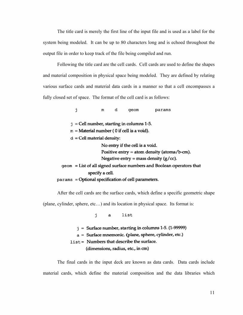
Following the title card are the cell cards. Cell cards are used to define the shapes
and material composition in physical space being modeled. They are defined by relating
various surface cards and material data cards in a manner so that a cell encompasses a
fully closed set of space. The format of the cell card is as follows:
After the cell cards are the surface cards, which define a specific geometric shape
(plane, cylinder, sphere, etc…) and its location in physical space. Its format is:
The final cards in the input deck are known as data cards. Data cards include
material cards, which define the material composition and the data libraries which
12
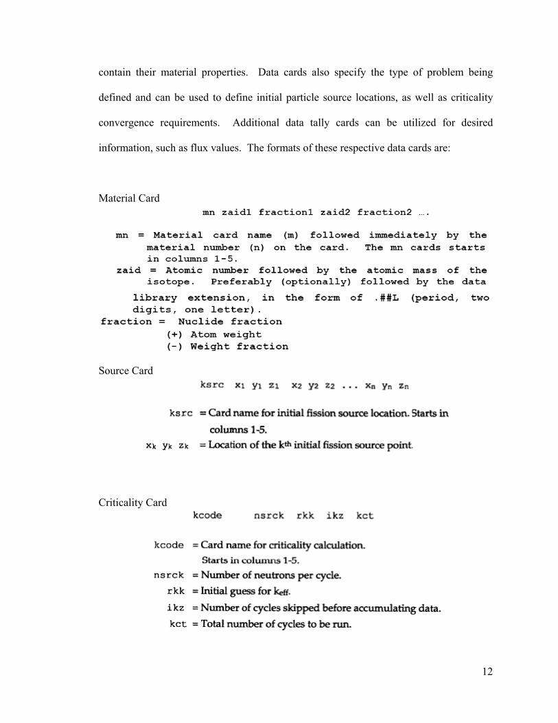
contain their material properties. Data cards also specify the type of problem being
defined and can be used to define initial particle source locations, as well as criticality
convergence requirements. Additional data tally cards can be utilized for desired
information, such as flux values. The formats of these respective data cards are:
Material Card
Source Card
Criticality Card
13
Further details and data card types can be found in the MCNP5 Criticality Primer
and MCNP5 Manual.
2.4 SCALE
Commissioned by the Nuclear Regulatory Commission in the late 1970s,
Software Computer Analyses for Licensing Evaluation (SCALE) was developed by Oak
Ridge National Laboratory. It incorporates several code packages in to one module
allowing for ease of use of various codes, focusing on applications related to nuclear fuel
facilities, and analysis for reactor licensing. SCALE is composed of various packages for
cross-section processing: BONAMI, NITAWL, CENTRM, PMC and XSDRNPM. Other
packages included are SCALE Material Optimization and REplacement Sequence
(SMORES), Tools for Sensitivity and UNcertainty Analysis Methodology
Implementation (TSUNAMI) in 1-D and 3-D, STandard Analysis for Reactivity for
BUrnup Credit using SCALE (STARBUCS), Criticality Safety Analysis Sequence
(CSAS) and the Monte Carlo KENO packages. CSAS6 for KENO-VI is newly
introduced to SCALE version 5.1 and provides for problem-dependent cross–section
processing and criticality calculations [SCALE: A Modular Code 2005]. KENO-VI
allows for more complicated geometry structures than KENO-Va, providing the ability to
create any geometry that can be defined by quadratic equations. Furthermore, KENO-VI
allows geometry intersections. Of particular interest is the ability to have surfaces that
share touching boundaries, a feature not available in KENO-Va. However, the new
features in SCALE-5.1 and KENO-VI packages have added costs. Specifically, there is a
decrease in detail that can be extracted and there is a significant increase in computational
costs. The issue of computational cost associated with KENO-VI is studied in detail in
14
Chapter 3. Chapter 4 addresses the decreased level of details, specifically involving
mesh limitations for flux distributions, which are present in the SCALE packages.
All SCALE packages can be controlled from setup and execution to results and
analysis using the Windows Graphical User Interface (GUI) known as Graphically
Enhanced Editing Wizard (GeeWiz). GeeWiz is a very user friendly GUI that allows a
beginner user of SCALE to quickly develop a model of their system. Through GeeWiz,
users are able to specify geometry, material composition, homogenization controls,
criticality tests and other useful modeling parameters. Various sample problems are
included in the SCALE manual [Scale: A Modular Code 2005] and the KENO-Va Primer
for Criticality [Busch and Bowman 2005].
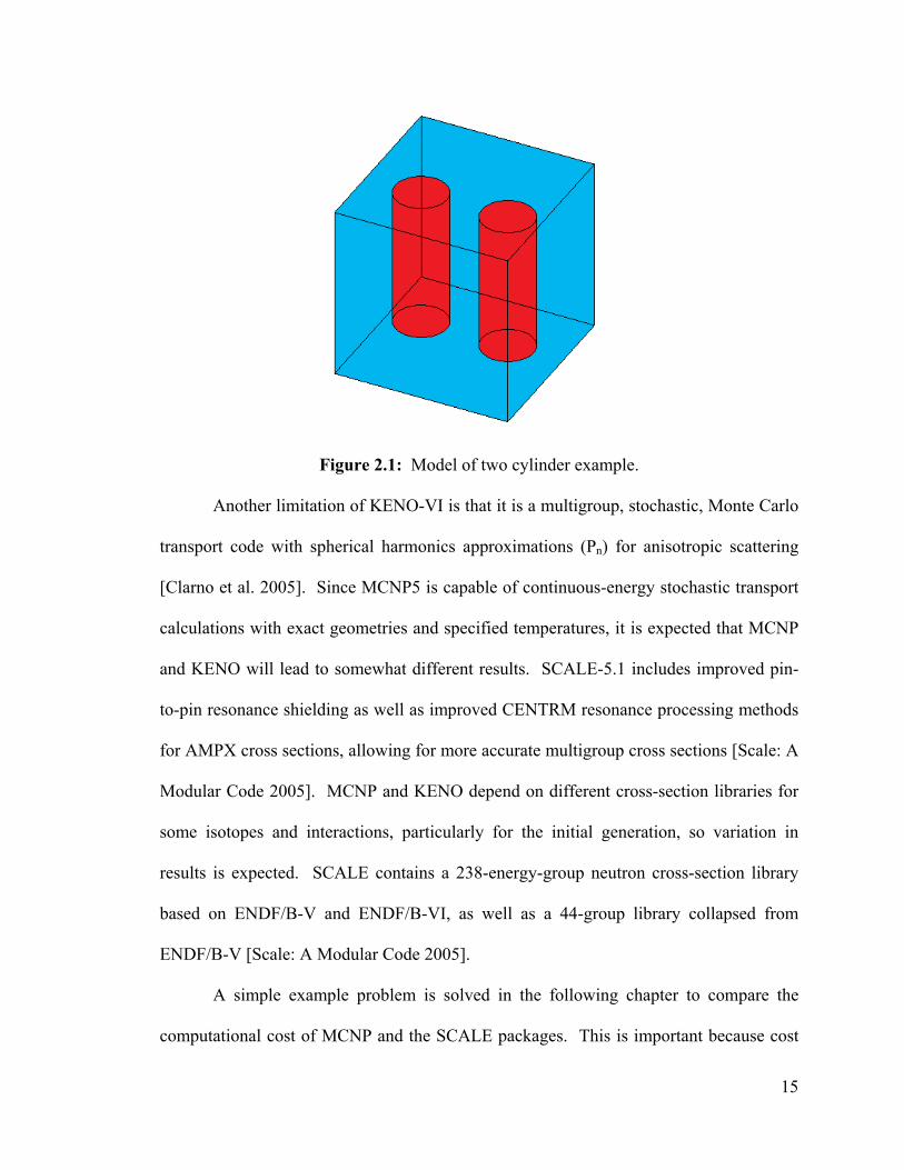
SCALE’s advantage is in its ease of use. SCALE is limited by geometries that it
can model, as well as by how the modeling can be done. SCALE is limited to composites
of rectangular, cylindrical or spherical shapes, though KENO-VI has made advances in
this area. Even more limiting is the fact that systems must be modeled with all new
shapes encompassing all shapes modeled earlier in the system. This means that no
individual shape can stand alone. An example of this is that two cylinders cannot be
modeled side-by-side but must instead be modeled inside a larger rectangular shape. This
simple model, shown in Figure 2.1, requires a three step approach. First, one of the
cylinders must be modeled as an individual geometric unit. Second, the other cylinder is
modeled as a region within the rectangular, or cuboid, unit. The second cylinder and the
cuboid are grouped as one geometric unit. The final, and third step is that the first
cylinder must be inserted (referred to as “hole” in SCALE terminology) into the cuboid
unit. This is necessary even if the cuboid unit, shown as blue in Figure 2.1, is vacuum.
15
Figure 2.1: Model of two cylinder example.
Another limitation of KENO-VI is that it is a multigroup, stochastic, Monte Carlo
transport code with spherical harmonics approximations (Pn) for anisotropic scattering
[Clarno et al. 2005]. Since MCNP5 is capable of continuous-energy stochastic transport
calculations with exact geometries and specified temperatures, it is expected that MCNP
and KENO will lead to somewhat different results. SCALE-5.1 includes improved pin-
to-pin resonance shielding as well as improved CENTRM resonance processing methods
for AMPX cross sections, allowing for more accurate multigroup cross sections [Scale: A
Modular Code 2005]. MCNP and KENO depend on different cross-section libraries for
some isotopes and interactions, particularly for the initial generation, so variation in
results is expected. SCALE contains a 238-energy-group neutron cross-section library
based on ENDF/B-V and ENDF/B-VI, as well as a 44-group library collapsed from
ENDF/B-V [Scale: A Modular Code 2005].
A simple example problem is solved in the following chapter to compare the
computational cost of MCNP and the SCALE packages. This is important because cost

16
and efficiency must also be considered when choosing the tools needed to accurately
model the F-Lattice.
17
Chapter 3: Computational Cost Comparisons
The computational cost associated with MCNP5 and the SCALE packages is
investigated in this chapter using a simple model of a core with plate fuel. The goal is to
determine the simulation conditions (mesh size, geometry, etc) under which one code is
more efficient than the other code. Sample input files for a SCALE-5.1/KENO-VI,
SCALE-5 KENO-Va and MCNP5 are provided in Appendix A.
3.1 Computational Time Comparisons
The SCALE packages are intended for ease of use and low computational cost.
However this comes at the loss of accuracy and limitations on geometries that can be
faithfully modeled. On the other hand, MCNP is intended for accurate simulations of
complex problems. It however, does not provide as user friendly an environment for
development as SCALE. Moreover, it is considered to have a very large computational
cost. The computational cost of the three codes is investigated as the model complexity
is increased. The following tests were performed.
Simulations for only basic k-effective calculations, as well as simulations for flux,
along with k-effective, calculations are carried out. Flux calculations require more
detailed evaluations in order to keep track of neutron fluence throughout the system.
These more detailed simulations are more computationally intensive than the simulations
for only k-effective calculations, but they provide additional, pertinent information. The
computational costs of simulations for only k-effective calculations are however
important because a large fraction of design and analysis simulations are for k-effective
only.
18
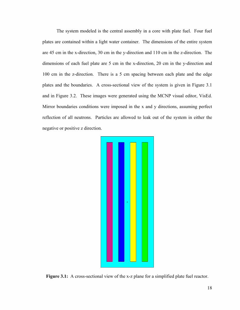
The system modeled is the central assembly in a core with plate fuel. Four fuel
plates are contained within a light water container. The dimensions of the entire system
are 45 cm in the x-direction, 30 cm in the y-direction and 110 cm in the z-direction. The
dimensions of each fuel plate are 5 cm in the x-direction, 20 cm in the y-direction and
100 cm in the z-direction. There is a 5 cm spacing between each plate and the edge
plates and the boundaries. A cross-sectional view of the system is given in Figure 3.1
and in Figure 3.2. These images were generated using the MCNP visual editor, VisEd.
Mirror boundaries conditions were imposed in the x and y directions, assuming perfect
reflection of all neutrons. Particles are allowed to leak out of the system in either the
negative or positive z direction.
Figure 3.1: A cross-sectional view of the x-z plane for a simplified plate fuel reactor.
19
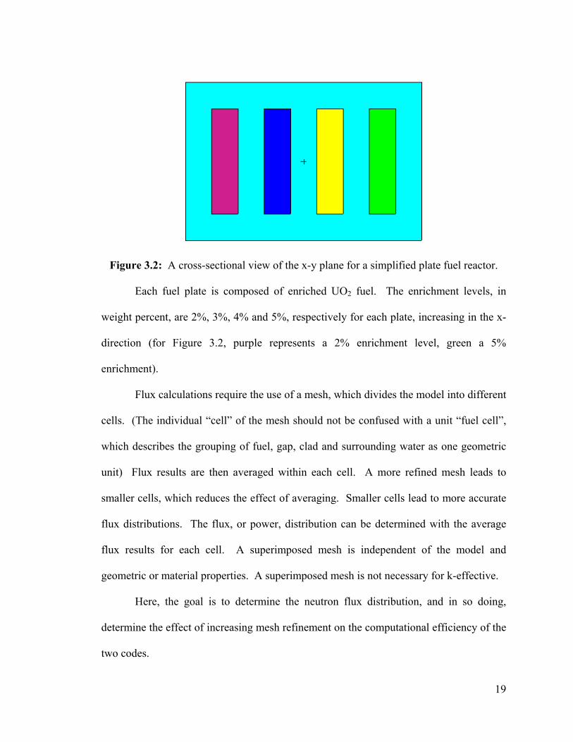
Figure 3.2: A cross-sectional view of the x-y plane for a simplified plate fuel reactor.
Each fuel plate is composed of enriched UO2 fuel. The enrichment levels, in
weight percent, are 2%, 3%, 4% and 5%, respectively for each plate, increasing in the x-
direction (for Figure 3.2, purple represents a 2% enrichment level, green a 5%
enrichment).
Flux calculations require the use of a mesh, which divides the model into different
cells. (The individual “cell” of the mesh should not be confused with a unit “fuel cell”,
which describes the grouping of fuel, gap, clad and surrounding water as one geometric
unit) Flux results are then averaged within each cell. A more refined mesh leads to
smaller cells, which reduces the effect of averaging. Smaller cells lead to more accurate
flux distributions. The flux, or power, distribution can be determined with the average
flux results for each cell. A superimposed mesh is independent of the model and
geometric or material properties. A superimposed mesh is not necessary for k-effective.
Here, the goal is to determine the neutron flux distribution, and in so doing,
determine the effect of increasing mesh refinement on the computational efficiency of the
two codes.
20
A superimposed mesh that covers only desired specific locations in the model can
be specified in MCNP5. Mesh cell size can be varied for each individual direction and
different size meshes can be placed in different parts of the system. The SCALE-5.1
package does not allow for a superimposed mesh. Instead, flux values are reported for
each geometry unit. This means that in order to obtain more spatially detailed results, the
model must be broken up into smaller constituent geometry units even if geometric units
are materially alike [Busch and Bowman 2005]. Additionally, fluxes are reported for all
units since there is no option to indicate only specific geometry units of the model where
flux results are desired.
Mesh refinement is introduced in the z-direction only. For MCNP5, this is a
simple task of increasing the mesh size in each fuel blade as the number of desired mesh
cells increases. For SCALE-5.1, this requires that smaller and smaller blocks of fuel be
used in the z direction. These smaller blocks are then stacked on top of each other to
develop a “mesh” of the complete fuel plate. These tests are carried out for KENO-Va
and KENO-VI inside the SCALE-5.1 package. [The importance of comparing KENO-
Va and KENO-VI is that KENO-VI was specifically developed for enhanced abilities to
handle more complex geometries.] The time required for each simulation is compared.
Increased CPU time indicates that more computer resources are needed for the
simulation.
It is important to note that the SCALE-5 package does allow superimposing a
mesh over the entire system. However, this mesh must have equal spacing in all
dimensions (uniform) and cannot be localized to specific locations. Due to the inability
to specify non-uniform mesh, or to define the mesh over only specific parts of the model,
21
a direct comparison of the SCALE-5 package cannot be made to the SCALE-5.1 package
for this model. Therefore a second set of tests were performed to directly compare the
performance of KENO-Va (within the SCALE-5 package) with MCNP5. Identical mesh
sizes are used in both codes, again with the objective of determining the computational
cost as a function of the grid size.
3.2 Efficiency Tests: MCNP5 and SCALE-5.1 (KENO-Va and KENO-
VI)
These tests were performed using a 2 GHz Intel Core2 CPU processor with 2 GB
of RAM. Simulations were carried out for 1, 2, 5, 10, 50 and 100 mesh cells in the z
direction, and with 1,000 and 10,000 particles. The 1, 2, 5, 10, 50 and 100 mesh cells
correlate to mesh sizes of 100 cm, 50 cm, 20 cm, 10 cm, 2 cm and 1 cm, respectively in
the z direction. The reported flux were averaged over the entire x-y plane of each
individual fuel plate (5 cm by 20 cm rectangle), the cross-sectional image shown in
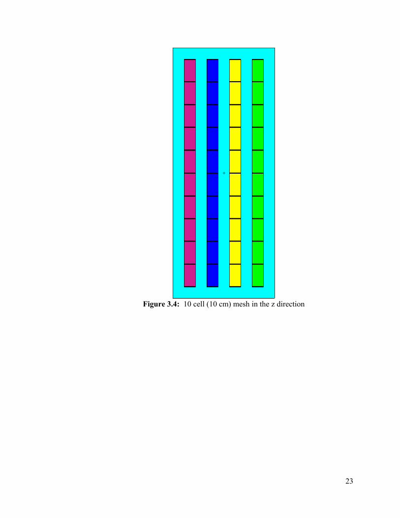
Figure 3.2. Examples of the meshes, in the z direction, for 5 cells (20 cm) and 10 cells
(10 cm) are shown in Figure 3.3 and Figure 3.4, respectively. Computational costs are
compared for the two codes in Fugre 3.5 and Figure 3.6.

22
Figure 3.3: 5 cell (20 cm) mesh in the z direction.
23
Figure 3.4: 10 cell (10 cm) mesh in the z direction
24
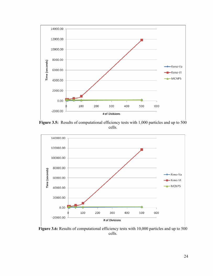
Figure 3.5: Results of computational efficiency tests with 1,000 particles and up to 500
cells.
Figure 3.6: Results of computational efficiency tests with 10,000 particles and up to 500
cells.
25
Results show that CPU time for MCNP5 remains essentially constant as mesh is
refined. KENO-Va shows a very slight increase in CPU time requirements as mesh
refinement is increased but remains less costly than MCNP5. Most interesting result is
that KENO-VI is the most computationally expensive even for coarse mesh, showing a
dramatic increase in CPU time as the number of cells increases. For a more relative
comparison of the two KENO codes, Figure 3.7 shows the ratio of the CPU time for the
two codes as a function of number of cells.
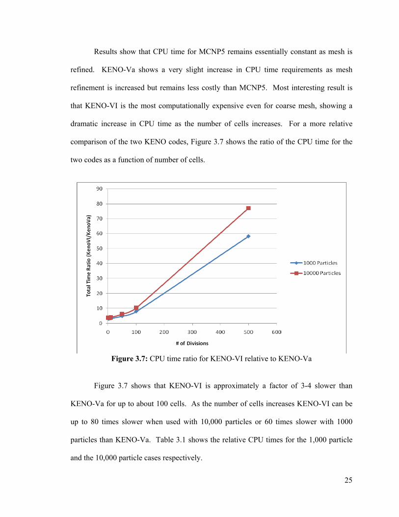
Figure 3.7: CPU time ratio for KENO-VI relative to KENO-Va
Figure 3.7 shows that KENO-VI is approximately a factor of 3-4 slower than
KENO-Va for up to about 100 cells. As the number of cells increases KENO-VI can be
up to 80 times slower when used with 10,000 particles or 60 times slower with 1000
particles than KENO-Va. Table 3.1 shows the relative CPU times for the 1,000 particle
and the 10,000 particle cases respectively.
26
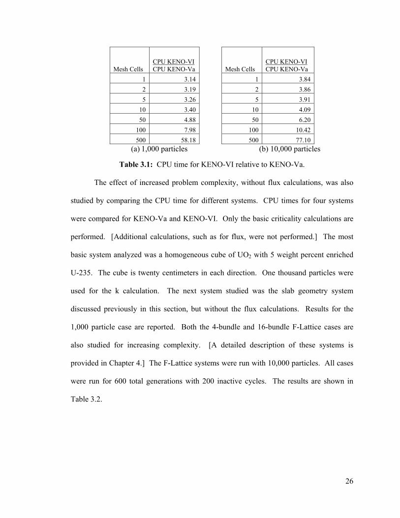
Mesh Cells CPU KENO-VI CPU KENO-Va Mesh Cells
CPU KENO-VI CPU KENO-Va
1 3.14 1 3.84 2 3.19 2 3.86 5 3.26 5 3.91
10 3.40 10 4.09 50 4.88 50 6.20
100 7.98 100 10.42 500 58.18 500 77.10
(a) 1,000 particles (b) 10,000 particles
Table 3.1: CPU time for KENO-VI relative to KENO-Va.
The effect of increased problem complexity, without flux calculations, was also
studied by comparing the CPU time for different systems. CPU times for four systems
were compared for KENO-Va and KENO-VI. Only the basic criticality calculations are
performed. [Additional calculations, such as for flux, were not performed.] The most
basic system analyzed was a homogeneous cube of UO2 with 5 weight percent enriched
U-235. The cube is twenty centimeters in each direction. One thousand particles were
used for the k calculation. The next system studied was the slab geometry system
discussed previously in this section, but without the flux calculations. Results for the
1,000 particle case are reported. Both the 4-bundle and 16-bundle F-Lattice cases are
also studied for increasing complexity. [A detailed description of these systems is
provided in Chapter 4.] The F-Lattice systems were run with 10,000 particles. All cases
were run for 600 total generations with 200 inactive cycles. The results are shown in
Table 3.2.
27
System
SCALE-5 KENO-Va Time (s)
SCALE-5.1 KENO-VI Time (s)
VI/Va Total Time
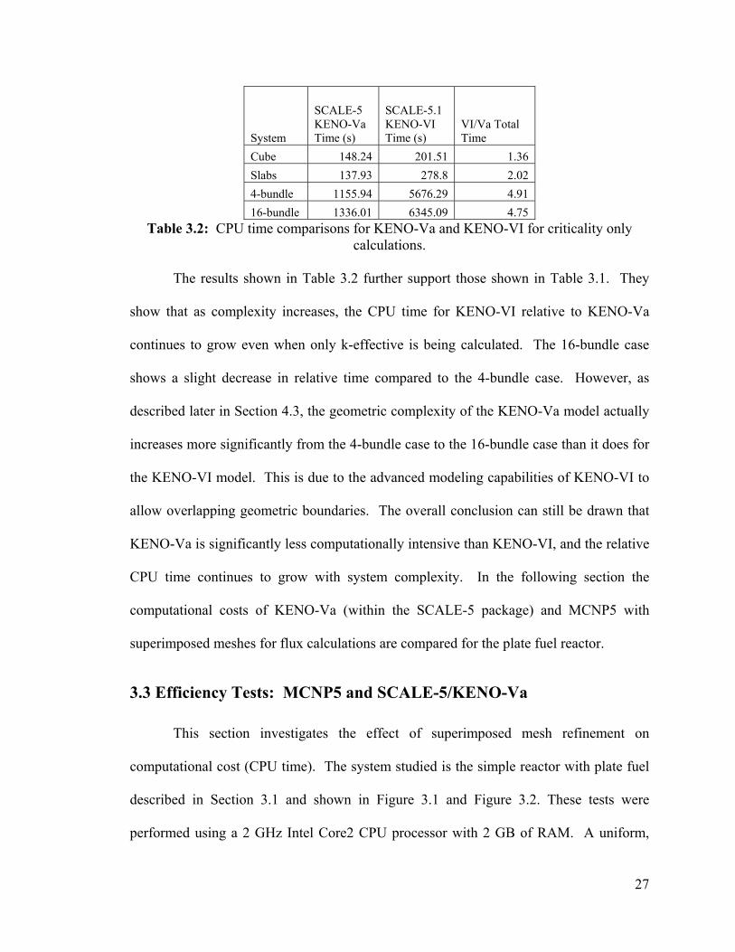
Cube 148.24 201.51 1.36 Slabs 137.93 278.8 2.02 4-bundle 1155.94 5676.29 4.91 16-bundle 1336.01 6345.09 4.75
Table 3.2: CPU time comparisons for KENO-Va and KENO-VI for criticality only calculations.
The results shown in Table 3.2 further support those shown in Table 3.1. They
show that as complexity increases, the CPU time for KENO-VI relative to KENO-Va
continues to grow even when only k-effective is being calculated. The 16-bundle case
shows a slight decrease in relative time compared to the 4-bundle case. However, as
described later in Section 4.3, the geometric complexity of the KENO-Va model actually
increases more significantly from the 4-bundle case to the 16-bundle case than it does for
the KENO-VI model. This is due to the advanced modeling capabilities of KENO-VI to
allow overlapping geometric boundaries. The overall conclusion can still be drawn that
KENO-Va is significantly less computationally intensive than KENO-VI, and the relative
CPU time continues to grow with system complexity. In the following section the
computational costs of KENO-Va (within the SCALE-5 package) and MCNP5 with
superimposed meshes for flux calculations are compared for the plate fuel reactor.
3.3 Efficiency Tests: MCNP5 and SCALE-5/KENO-Va
This section investigates the effect of superimposed mesh refinement on
computational cost (CPU time). The system studied is the simple reactor with plate fuel
described in Section 3.1 and shown in Figure 3.1 and Figure 3.2. These tests were
performed using a 2 GHz Intel Core2 CPU processor with 2 GB of RAM. A uniform,
28
superimposed mesh is imposed for k-effective and flux calculations. The mesh is over
the entire system and has equal spacing in all directions. Mesh refinement was performed
with 50 cm, 20 cm, 10 cm, 5 cm, 2 cm and 1 cm cell size spacing used in all directions.
As cell size is decreased, the number of mesh points increases, providing a more accurate
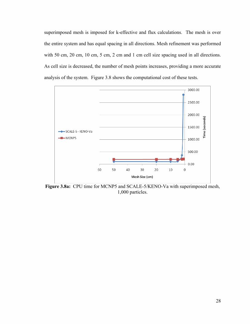
analysis of the system. Figure 3.8 shows the computational cost of these tests.
Figure 3.8a: CPU time for MCNP5 and SCALE-5/KENO-Va with superimposed mesh,
1,000 particles.

29
Figure 3.8b: CPU time for MCNP5 and SCALE-5/KENO-Va with superimposed mesh,
10,000 particles.
All tests showed good accuracy in calculated multiplcation factors. The 1,000
particle simulations resulted in a k of 0.9388 for KENO-Va and 0.9321 for MCNP5. The
10,000 particlue simulations resulted in a k of 0.9436 for KENO-Va and 0.9319 for
MCNP5 (Results are not affected by mesh size). The accuracy, as determined by
Equation 4.2 in Section 4.7, of the k-effective values is within 0.71% and 1.26% for the
1,000 particle and 10,000 particle simulations, respectively. The techniques necessary to
compare the results of the flux calculations of the two codes are given in Chapter 4.
With strong agreement in results, the important feature of these tests is the variation in
computational cost. Figure 3.8a (1,000 particles) and Figure 3.8b (10,000 particles) both
show that CPU time for KENO-Va, in SCALE-5, for very coarse meshes is shorter than
that for MCNP5. It is when the mesh starts to become highly refined that SCALE-5
begins to dramatically increase in computational cost. Figure 3.8a shows that with 1,000
particles MCNP5 becomes more efficient at a cell size of 2 cm. Figure 3.8b shows that
30
for a higher number of particles, 10,000 particles per generation, KENO-Va remains
more efficient than MCNP5 for a 1 cm or larger mesh. The dramatic increase in CPU
time is a result of temporary memory (RAM) limitations. A large increase in
computational cost, or increase in run-time, occurs when the computer must utilize the
harddrive as virtual memory. [Virtual memory allows for the use of additional temporary
memory when it is required beyond the storage capacity of the RAM.] The effect of
using virtual memory can be an increase as large as an order of magnitude for runtime
[Landau et al. 2007], as illustrated in Figure 3.8.
It is important to note that it is because of the output format of the SCALE-5 mesh
file that RAM space quickly gets used up and harddrive must be used as virtual memory.
At a 1 cm cell, this simple model produced an output text file that was over 2 GB in size.
No standard text editor was able to open this size text file and it was neccesary to use a
program called “Large Text File Viewer 4u” [SwiftGear 2005] to read the output.
Additionally, for the 1 cm mesh case, the code was unable towrite all the information and
close the files, and hence the criticality information was not ouputted, leaving out crucial
data in this simulation. Mesh refinement could not be carried any further due to these
limitations.
3.4 Efficiency Tests Conclusions
The efficiency tests for MCNP5, KENO-Va in SCALE-5.1 and KENO-VI in
SCALE-5.1 provided very clear results. With the ability to provide localized, well-
defined meshes, MCNP5 is able to maintain a near constant computational cost as more
spatially refined detailed information is desired. Computational cost for KENO-VI in
SCALE-5.1 dramatically increases as geometric complexity increases. This is due to the
31
generalized nature of the code, which quickly negates the benefits of more complex
geometry features. The computational cost for KENO-Va in SCALE-5.1 only slightly
increases with geometric complexity but remains below that of MCNP5. These results
suggest that KENO-Va is the most cost-effective code for this type of simulation.
Perhaps most interesting is the information provided in Figure 3.5. The SCALE
manual states that a system that can be modeled in both KENO-Va and KENO-VI will
“typically run twice as long in KENO-VI as in KENO-Va” [SCALE: A Modular Code
2005]. It suggests using KENO-VI only for systems that cannot be modeled in KENO-
Va. However, Figure 3.7 shows that the CPU time for KENO-VI relative to KENO-Va
grows with finer mesh, eliminating any advantage in using KENO-VI, especially when
MCNP5 can be utilized for greater detail. A significant increase in CPU time for basic k-
effective calculations was also shown in Table 3.2.
The MCNP5 and KENO-Va (within SCALE-5) tests further verified that KENO-
Va is less computationally intensive for coarse mesh calculations. A dramatic increase in
computing time was seen once the mesh refinement reached a certain point that overtaxed
the temporary memory available. The rapid increase in computing time seen with
KENO-Va (within SCALE-5) was most likely due to the code’s needs exceeding the
available 2 GB RAM. These limits were reached with meshes that were still fairly
coarse. This was because of the inability to: 1) Specify non-uniform mesh; 2) Specify the
mesh only in regions where the flux or power distribution is needed.
These efficiency tests show that KENO-Va within the SCALE package should
only be used when quick basic results, including relatively coarse meshes for flux
calculations, are desired. However, for very complex geometries and analysis that calls
32
for detailed flux information, it would be computationally cost effective to utilize
MCNP5.
The following chapter provides a detailed background on the F-Lattice.
Additionally, the accuracy of KENO-VI (within SCALE-5.1) and KENO-Va (within
SCALE-5) are evaluated by comparing their results to those obtained using MCNP5.
33
Chapter 4: The F-Lattice
First, a detailed description of the main features of the F-Lattice design is given.
The F-Lattice is then modeled and analyzed using MCNP5, SCALE-5.1/KENO-VI and
SCALE-5/KENO-Va. The ability to accurately calculate the system’s effective
multiplication factor using the KENO codes is validated in this chapter. The necessary
steps to compare the results of the neutron flux calculations are developed and the results
for SCALE-5/KENO-Va and MCNP5 are compared.
4.1 The F-Lattice
The Four-Bundle Lattice, known as the F-Lattice, is an innovative design that
reduces the total number of control blades employed in the reactor design. Standard
lattice designs, sometimes referred to as the N-Lattice, have control blades located every
other fuel bundle. While the width of each control blade varies with design, they are
smaller than bundle pitch. An earlier modification, known as the K-Lattice, employed a
staggered row configuration. The result is that each individual fuel bundle is effectively
enclosed by control blades on all four sides [Challberg 1998]. The K-Lattice is intended
to improve control rod worth, a concern in some early GE BWR designs that utilized
stainless steel clad. The K-Lattice also implemented an increased control rod pitch and
larger fuel assembly. It was seen that the K-Lattice was most beneficial with increased
fuel assembly size, a larger pitch and wider control blades. Increasing the size of the fuel
assemblies, pitch and control blade width helped reduce power peaking that resulted from
the staggered row configuration [Challberg 1998]. The F-Lattice was adapted directly
from the K-Lattice with these ideas in mind.
34
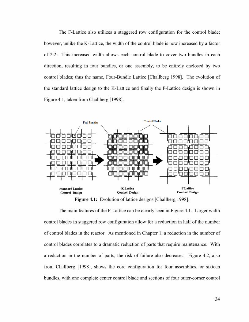
The F-Lattice also utilizes a staggered row configuration for the control blade;
however, unlike the K-Lattice, the width of the control blade is now increased by a factor
of 2.2. This increased width allows each control blade to cover two bundles in each
direction, resulting in four bundles, or one assembly, to be entirely enclosed by two
control blades; thus the name, Four-Bundle Lattice [Challberg 1998]. The evolution of
the standard lattice design to the K-Lattice and finally the F-Lattice design is shown in
Figure 4.1, taken from Challberg [1998].
Figure 4.1: Evolution of lattice designs [Challberg 1998].
The main features of the F-Lattice can be clearly seen in Figure 4.1. Larger width
control blades in staggered row configuration allow for a reduction in half of the number
of control blades in the reactor. As mentioned in Chapter 1, a reduction in the number of
control blades correlates to a dramatic reduction of parts that require maintenance. With
a reduction in the number of parts, the risk of failure also decreases. Figure 4.2, also
from Challberg [1998], shows the core configuration for four assemblies, or sixteen
bundles, with one complete center control blade and sections of four outer-corner control

35
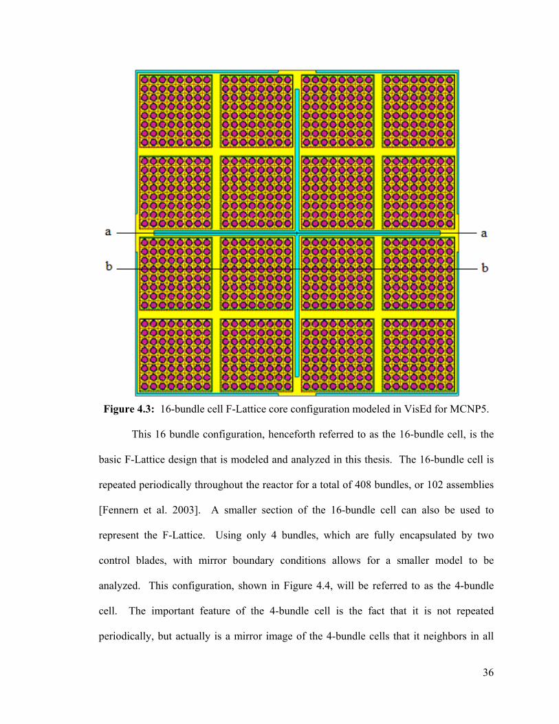
blades. Figure 4.3 is an additional view of this configuration when modeled with
MCNP5.
Figure 4.2: 16-bundle F-Lattice core configuration [Challberg 1998].
36
Figure 4.3: 16-bundle cell F-Lattice core configuration modeled in VisEd for MCNP5.
This 16 bundle configuration, henceforth referred to as the 16-bundle cell, is the
basic F-Lattice design that is modeled and analyzed in this thesis. The 16-bundle cell is
repeated periodically throughout the reactor for a total of 408 bundles, or 102 assemblies
[Fennern et al. 2003]. A smaller section of the 16-bundle cell can also be used to
represent the F-Lattice. Using only 4 bundles, which are fully encapsulated by two
control blades, with mirror boundary conditions allows for a smaller model to be
analyzed. This configuration, shown in Figure 4.4, will be referred to as the 4-bundle
cell. The important feature of the 4-bundle cell is the fact that it is not repeated
periodically, but actually is a mirror image of the 4-bundle cells that it neighbors in all
37
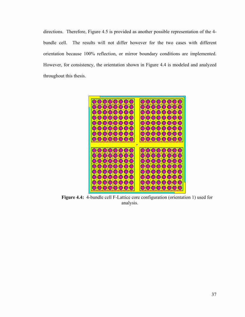
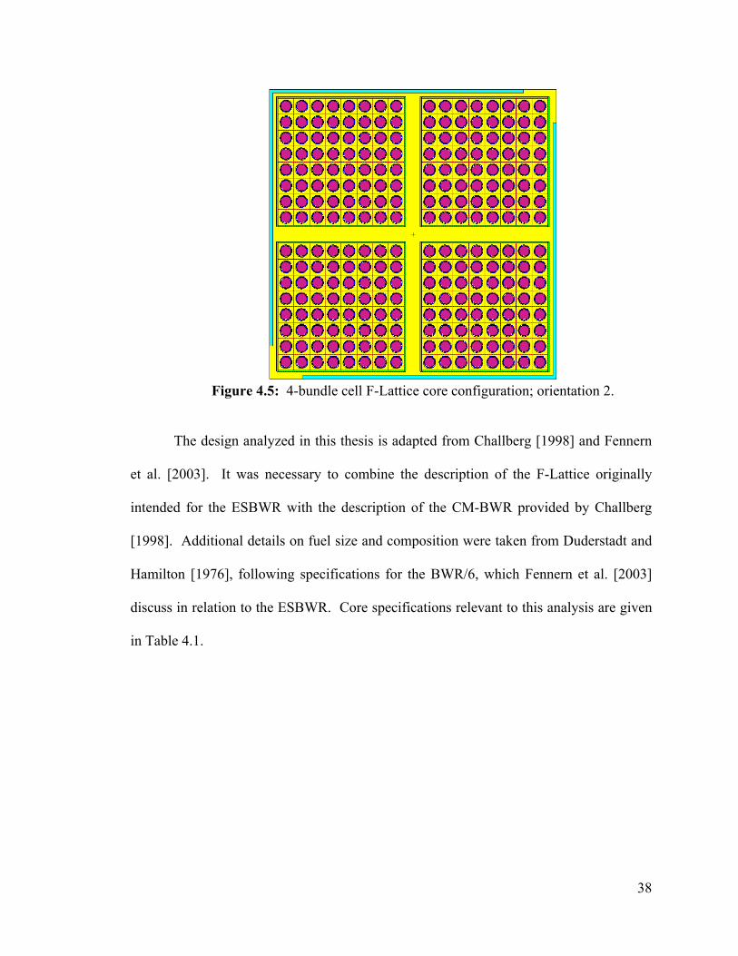
directions. Therefore, Figure 4.5 is provided as another possible representation of the 4-
bundle cell. The results will not differ however for the two cases with different
orientation because 100% reflection, or mirror boundary conditions are implemented.
However, for consistency, the orientation shown in Figure 4.4 is modeled and analyzed
throughout this thesis.
Figure 4.4: 4-bundle cell F-Lattice core configuration (orientation 1) used for
analysis.
38
Figure 4.5: 4-bundle cell F-Lattice core configuration; orientation 2.
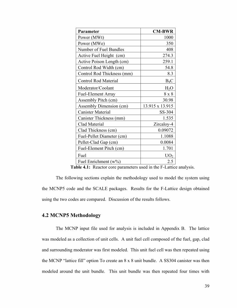
The design analyzed in this thesis is adapted from Challberg [1998] and Fennern
et al. [2003]. It was necessary to combine the description of the F-Lattice originally
intended for the ESBWR with the description of the CM-BWR provided by Challberg
[1998]. Additional details on fuel size and composition were taken from Duderstadt and
Hamilton [1976], following specifications for the BWR/6, which Fennern et al. [2003]
discuss in relation to the ESBWR. Core specifications relevant to this analysis are given
in Table 4.1.
39
Parameter CM-BWR Power (MWt) 1000 Power (MWe) 350 Number of Fuel Bundles 408 Active Fuel Height (cm) 274.3 Active Poison Length (cm) 259.1 Control Rod Width (cm) 54.8 Control Rod Thickness (mm) 8.3 Control Rod Material B4C Moderator/Coolant H2O Fuel-Element Array 8 x 8 Assembly Pitch (cm) 30.98 Assembly Dimension (cm) 13.915 x 13.915 Canister Material SS-304 Canister Thickness (mm) 1.535 Clad Material Zircaloy-4 Clad Thickness (cm) 0.09072 Fuel-Pellet Diameter (cm) 1.1088 Pellet-Clad Gap (cm) 0.0084 Fuel-Element Pitch (cm) 1.701 Fuel UO2 Fuel Enrichment (w%) 2.5
Table 4.1: Reactor core parameters used in the F-Lattice analysis.
The following sections explain the methodology used to model the system using
the MCNP5 code and the SCALE packages. Results for the F-Lattice design obtained
using the two codes are compared. Discussion of the results follows.
4.2 MCNP5 Methodology
The MCNP input file used for analysis is included in Appendix B. The lattice
was modeled as a collection of unit cells. A unit fuel cell composed of the fuel, gap, clad
and surrounding moderator was first modeled. This unit fuel cell was then repeated using
the MCNP “lattice fill” option To create an 8 x 8 unit bundle. A SS304 canister was then
modeled around the unit bundle. This unit bundle was then repeated four times with
40
moderator spacing between them. This was done using the “like m but” command in
MCNP. This command allows a unit to be repeated with slight changes in material or
physical location. The control rods were then modeled around the four bundles. This
completed the 4-bundle cell. The 4-bundle cell was then repeated, as well as rotated as
needed, to create the 16-bundle cell.
The source used was the “ksrc”, which allows the user to define specific locations
for the initial sources to be located. Sources were placed in the center of several different
fuel rods throughout the system. MCNP5 automatically expands its source locations with
each generation history, using information from each previous history to better
approximate the next. Finally, the F4 tally was utilized for the flux analysis. As
discussed in Chapter 3, MCNP5 allows a user-defined superimposed mesh for the flux
calculations (The F4 tally). Energy levels can also be specified with the F4 tally [X-5
Monte Carlo Team 2003]. Thermal, epithermal, fast and total neutron fluxes were
monitored. The energy groups were 0 - 0.225 eV for thermal neutrons, 0.225 eV – 0.1
MeV for epithermal neutrons and 0.1 MeV and above for fast neutrons. The F4 flux tally
results are outputted in a second file different from the standard output. Normalization
techniques are discussed in Section 4.6.
4.3 SCALE-5.1/KENO-VI Methodology
The SCALE input code used for analysis is included in Appendix B. As
discussed in Chapter 2 and Chapter 3, the SCALE package requires that each geometric
unit be built surrounding the previous units. Thus, the initial approach to model the F-
Lattice using SCALE-5.1/KENO-VI is similar to that for the MCNP5 code. A unit fuel
cell composed of fuel, gap, clad and water moderator is first created. The SCALE

41
package utilizes arrays, filled with geometric units, to repeat the structures. This allows
the unit fuel cell to be repeated in an 8 x 8 array, which can then be encapsulated in the
stainless steel canister, creating a unit bundle. The unit bundle can then be repeated in an
array four times. The SCALE package allows for additional geometric units, referred to
as “holes”, to be inserted as desired into the system. As discussed in Chapter 2, KENO-
VI allows for these holes to have overlapping boundaries with other geometric units.
This allows for the 4-bundle cell, and eventually the 16-bundle cell, to be modeled
directly in the same fashion as in MCNP. The 4-bundle cell can then be repeated and
rotated in a 2 x 2 array to create the 16-bundle cell. It is important to note that rotating
the 4-bundle cell orientation actually requires an entirely new 4-bundle to be modeled,
since there is no command available to rotate or “flip” a geometric unit; this is also the
case in MCNP5.
While modeled fairly simply using KENO-VI, it is important to keep in mind the
limitations discussed in Chapter 3. KENO-VI cannot evaluate fluxes with a user-defined
superimposed mesh. In order to determine the local reaction rates, geometric units must
be broken down (when the geometry is built) in to smaller and smaller units, which
increasingly become more computationally expensive. The SCALE-5.1 package slows
down (compared to MCNP5) when more spatially detailed flux distributions are desired.
As an example, the 4-bundle cell case was developed that used 100 divisions along the z-
axis only within the fuel cells. That is the control blades were still treated as a single
unit. This corresponds to a coarse mesh of 2.743 cm in just the z-direction and only
within the fuel cells. However, the time required to complete this run was 116642.12
seconds (over 1 day and 8 hours). On the other hand, MCNP5, using a superimposed
42
mesh, yields extremely refined levels of detail in 7 and 16 hours for 4-bundle cell and 16-
bundle cell, respectively. However, as shown in Chapter 3, KENO-Va still maintains a
computational advantage over MCNP5 for most levels of detail. Therefore, it is desirable
to develop techniques to use the SCALE-5/KENO-Va package to model the system.
4.4 SCALE-5/KENO-Va Methodology
KENO-Va is capable of calculating fluxes with a user-defined superimposed
mesh but has limitations in modeling systems that involve geometric units that have
overlapping boundaries. To overcome this difficulty, it was necessary to break the 4-
bundle cell and 16-bundle into smaller pieces which could then be combined together in
multiple sets of arrays. This approach is much more difficult and complicated compared
to the KENO-VI approach. For the 4-bundle case, the number of geometric units
required increases from 5 units and 1 array to 25 units and 5 arrays. The 16-bundle case
increases from 7 units and 2 arrays to 32 units and 8 arrays. Sample input files for both
KENO-VI and KENO-Va are included for the 4-bundle and 16-bundle cases in Appendix
B.
The advantages that KENO-Va provides in both computational cost, as outlined in
Chapter 3, as well as the ability to utilize a superimposed mesh for flux calculations far
outweigh the relative disadvantages in geometry modeling. The mesh level flux results
are included in the standard SCALE output file broken down by unit, region and energy.
Also, when comparing flux values it is important to keep in mind that the SCALE-5
superimposed mesh is over the entire model and cannot be uniquely defined for each
dimension. The SCALE-5 mesh extends beyond the boundaries of the model if part of a
unit is present in the cell. An example is a mesh size of 10 cm for a model that is 10.10
43
cm long in one of the dimensions. SCALE-5 will have 2 cells in the mesh despite the
fact that the second cell is 99% void. For comparison, it is necessary to adjust the
MCNP5 mesh accordingly to be the same as that for the SCALE output. The techniques
required to compile and compare flux values with MCNP5 results are detailed in the
following section.
4.5 Flux Output and Perl
A literature search found no previous work on the SCALE-5/KENO-Va flux
calculations using a superimposed mesh. Superimposed mesh has been used to evaluate
leakage rates or for increased accuracy in perturbation studies [SCALE: A Modular Code
2005]. Moreover, when fluxes were reported, they were in per unit lethargy units
[Johnson and Clarno 2007]. For this reason, SCALE-5/KENO-Va spatial flux results
have not previously been compared to results obtained with another code, such as
MCNP5. The necessary approach to make such a comparison for SCALE-5 and MCNP5
are developed in this section.
The KENO-Va flux results file is very large. Moreover, the flux results are
broken down by geometric units, regions, energy and cell in the mesh. A single unit fuel
cell that has four regions (fuel, gap, clad and moderator) and only one cell of the
superimposed mesh is a good example of the output’s complexity. Even though only one
cell in the mesh contains the entire unit fuel cell, each region is reported individually for
that cell. With 238 energy levels this results in 952 flux values (4 regions multiplied by
238 energy groups) reported for a single cell. The output is further complicated by the
fact that some cells can include multiple units. Results for the same cell are then
reported in multiple locations in the output file. Additionally, the output is reported in
44
mesh grid locations, despite being defined by mesh cell size in centimeters. These mesh
grid locations must be transformed to the Cartesian grid to allow comparison with
MCNP5 results. The final difficulty related to the mesh flux values are the reported
units. As discussed in Section 4.5, MCNP5 reports flux values normalized to “per
starting particle.” However, the SCALE-5 values are normalized to “per unit volume per
starting particle” [SCALE: A Modular Code 2005]. “Unit volume” refers to the
geometric “region” within the unit that is within the specific cell for which the flux value
is reported. In the SCALE-5 terminology, a “region” is a geometric shape that is
contained within a larger “unit.” The approach followed here is to normalize the
SCALE-5 flux values to “per starting particle”, which are then scaled to the proper units
of neutrons per centimeter squared per second following Equation 4.1, described in
Section 4.6.
With a very complicated and seemingly disorganized output file, it becomes
necessary to develop an efficient way to organize and sum all the flux values in order to
obtain a single total flux for each individual cell of the mesh.
Practical Extraction and Report Language (Perl) is a scripting language
that is used for parsing large data sets into more manageable and easier to analyze results
[Lemey and Colburn 2002]. Perl can be used on all major operating systems with no
changes necessary to the input file. It is an open source scripting language that can be
obtained free of charge from many online locations; the main provider being
www.ActiveState.com. Its ease of programming and ability to quickly parse data sets
provide ideal abilities to extract desired results from the KENO-Va output. The script,
FluxParse.pl, was written in Perl to analyze the output file for any arbitrary sized mesh
45
for any geometry modeled in SCALE-5/KENO-Va. FluxParse.pl is included in
Appendix C along with simple test case results for verification. The comments in
FluxParse.pl explain the one-line command necessary to run the script from the OS
command line (DOS for Windows).
The script, FluxParse.pl, sums all the flux values for a single cell together to
report a single total neutron flux value. To address the issue of “per unit volume”
discussed above, it is necessary to first extract the total volume for each region as
calculated by SCALE-5. Total volume information is reported in the “sum of mesh
volumes for each region” table in the output file. An “average volume” (per cell) is then
evaluated by dividing the total volume by the number of times each region appears in the
model. An example of how the “sum of mesh volumes for each region” table appears in
the output file is shown in Figure 4.6.
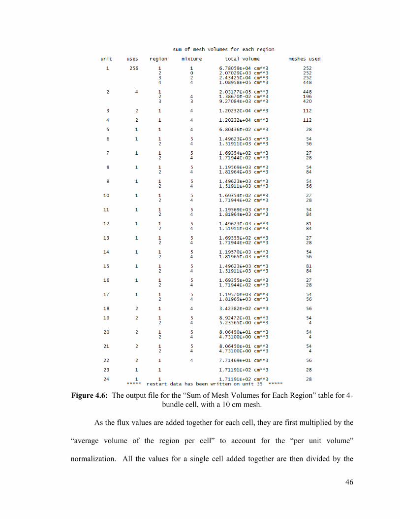
46
Figure 4.6: The output file for the “Sum of Mesh Volumes for Each Region” table for 4-
bundle cell, with a 10 cm mesh.
As the flux values are added together for each cell, they are first multiplied by the
“average volume of the region per cell” to account for the “per unit volume”
normalization. All the values for a single cell added together are then divided by the
47
mesh block volume (1000 cm^3 for a 10 cm mesh). A separate tab delimited text file,
Flux.txt, is then created containing results normalized to “per starting particle”, the same
as the MCNP5 flux tallies. Flux.txt can be opened by a spreadsheet editor, such as Excel.
The output is organized in the same, increasing (x, y, z) order format that is used by the
MCNP5 mesh output. Transformation to a Cartesian grid system can then be carried out
manually. However, if a similarly sized mesh is used in an MCNP5 run, then the
MCNP5 grid will be the same and can be used directly for both codes for comparison.
(The Perl script can easily be modified to incorporate the transformation to the Cartesian
grid if desired.)
Error is introduced in this process due to the use of the average volume of each
region per cell. Depending on the system being modeled and the mesh size utilized, each
cell contains different fractions of “region volume”. Using the average volume assumes
that the same amount of “region volume” appears in each cell that the region is in. More
accurate analysis would take the varying “region volumes” in to account for each specific
cell. However, since “region volume” is not reported for each cell of the mesh, the
average values are used, leading to a volume averaging error. To eliminate this error
would require a manual calculation of “region volume” for each specific model and mesh
size, a task that would be very tedious. Section 4.7 and Section 4.8 provide further
discussion of how this averaging error manifests itself in the results.
4.6 Flux Normalization
The flux output for MCNP5 is normalized with “per starting particle” and must be
converted into “real” fluxes. The SCALE-5 values in Flux.txt are also normalized with
48
“per starting particle”. Flux with the units of number of neutrons per centimeter squared
per second is computed as [Tari 1994].
Neutron Flux sec
#2cm
= Tallied Quantity effkqQ
P υ⋅⋅×
1 (4.1)
• P = Thermal reactor power in MW (1000 MWt)
• Q = Energy released per fission, MeV (200 MeV)
• q =1.602x10⁻¹⁹ joules per eV, conversion factor
• υ = Average number of neutrons released per fission, determined by
MCNP/SCALE
• effk = Effective neutron multiplication number, determined by MCNP/SCALE
4.7 MCNP & SCALE Comparison Results
The 4-bundle and 16-bundle cases were run using MCNP5, SCALE-5.1/KENO-
VI and SCALE-5/KENO-Va. The results of the three codes are compared. Relative
percent differences are reported,
Relative % Difference = xxx resultsSCALE )( _ −
x 100% (4.2)
where the absolute value is not taken in order to preserve the positive or negative
correlations. Fluxes are reported in the units of number of neutrons per centimeter
squared per second as dictated by Equation 4.1. The variance and standard deviation
between the flux values are normalized to the unit interval, following Equation 4.3 and
Equation 4.4:
49
Variance σ2 = ∑=
Φ−ΦN
i
testii
N1
2)( (4.3)
Standard Deviation σ = ∑=
Φ−ΦN
i
testii
N1
2)( (4.4)
where N is the total number of cells in the mesh and i sums over all cells. All codes were
run for an acceptably small standard deviation of the effective multiplication factor,
always less than 0.001. The 16-bundle MCNP5 case was run with 50,000 particles for
250 inactive cycles and 350 active cycles. The 4-bundle MCNP5 case used 100,000
particles for 250 inactive cycles and 550 active cycles. More particles and histories were
used in the 4-bundle case for evaluation of the flux distribution, which requires more
information than the k-effective calculations. Flux distributions were not analyzed in the
16-bundle case. The SCALE-5.1/KENO-VI cases were both run with 10,000 particles
for 200 inactive cycles and 400 active cycles. The SCALE-5/KENO-Va cases were all
run with 10,000 particles for 250 inactive cycles and 550 active cycles. More histories
were used for KENO-Va than KENO-VI to guarantee accurate flux calculations. An
additional test of a single unit fuel cell is included to give basis of comparison for the
more complicated F-Lattice. These trials were run in the SCALE packages with 1000
particles for 3 inactive cycles and 200 active cycles. The unit fuel cell case was run in
MCNP5 using 500 particles for 100 inactive cycles and 200 active cycles.
The results, including standard deviation, for the unit fuel cell are shown in Table
4.2. The unit fuel cell results are included to show the level of agreement between the
SCALE packages results and MCNP5 results for a simple system. Similar agreement is
desirable for the F-Lattice simulations.
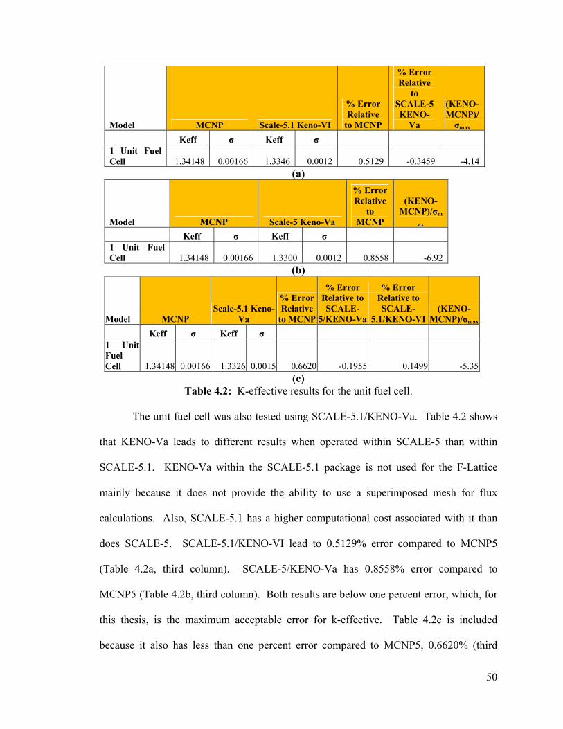
50
Model MCNP Scale-5.1 Keno-VI
% Error Relative
to MCNP
% Error Relative
to SCALE-5 KENO-
Va
(KENO-MCNP)/σmax
Keff σ Keff σ 1 Unit Fuel Cell 1.34148 0.00166 1.3346 0.0012 0.5129 -0.3459 -4.14
(a)
Model MCNP Scale-5 Keno-Va
% Error Relative
to MCNP
(KENO-MCNP)/σm
ax Keff σ Keff σ 1 Unit Fuel Cell 1.34148 0.00166 1.3300 0.0012 0.8558 -6.92
(b)
Model MCNP Scale-5.1 Keno-
Va
% Error Relative
to MCNP
% Error Relative to SCALE-
5/KENO-Va
% Error Relative to SCALE-
5.1/KENO-VI (KENO-
MCNP)/σmax
Keff σ Keff σ 1 Unit Fuel Cell 1.34148 0.00166 1.3326 0.0015 0.6620 -0.1955 0.1499 -5.35
(c) Table 4.2: K-effective results for the unit fuel cell.
The unit fuel cell was also tested using SCALE-5.1/KENO-Va. Table 4.2 shows
that KENO-Va leads to different results when operated within SCALE-5 than within
SCALE-5.1. KENO-Va within the SCALE-5.1 package is not used for the F-Lattice
mainly because it does not provide the ability to use a superimposed mesh for flux
calculations. Also, SCALE-5.1 has a higher computational cost associated with it than
does SCALE-5. SCALE-5.1/KENO-VI lead to 0.5129% error compared to MCNP5
(Table 4.2a, third column). SCALE-5/KENO-Va has 0.8558% error compared to
MCNP5 (Table 4.2b, third column). Both results are below one percent error, which, for
this thesis, is the maximum acceptable error for k-effective. Table 4.2c is included
because it also has less than one percent error compared to MCNP5, 0.6620% (third
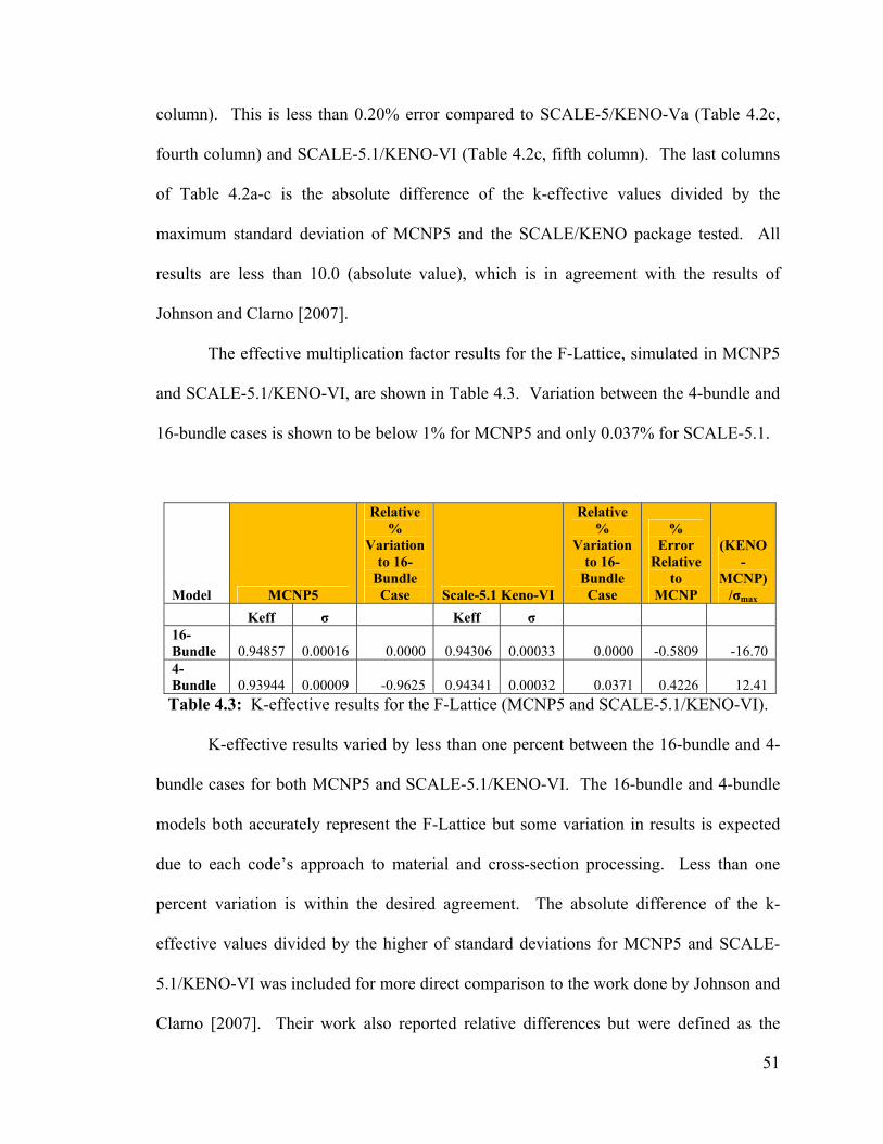
51
column). This is less than 0.20% error compared to SCALE-5/KENO-Va (Table 4.2c,
fourth column) and SCALE-5.1/KENO-VI (Table 4.2c, fifth column). The last columns
of Table 4.2a-c is the absolute difference of the k-effective values divided by the
maximum standard deviation of MCNP5 and the SCALE/KENO package tested. All
results are less than 10.0 (absolute value), which is in agreement with the results of
Johnson and Clarno [2007].
The effective multiplication factor results for the F-Lattice, simulated in MCNP5
and SCALE-5.1/KENO-VI, are shown in Table 4.3. Variation between the 4-bundle and
16-bundle cases is shown to be below 1% for MCNP5 and only 0.037% for SCALE-5.1.
Model MCNP5
Relative %
Variation to 16-
Bundle Case Scale-5.1 Keno-VI
Relative %
Variation to 16-
Bundle Case
% Error
Relative to
MCNP
(KENO-
MCNP)/σmax
Keff σ Keff σ 16-Bundle 0.94857 0.00016 0.0000 0.94306 0.00033 0.0000 -0.5809 -16.70 4-Bundle 0.93944 0.00009 -0.9625 0.94341 0.00032 0.0371 0.4226 12.41 Table 4.3: K-effective results for the F-Lattice (MCNP5 and SCALE-5.1/KENO-VI).
K-effective results varied by less than one percent between the 16-bundle and 4-
bundle cases for both MCNP5 and SCALE-5.1/KENO-VI. The 16-bundle and 4-bundle
models both accurately represent the F-Lattice but some variation in results is expected
due to each code’s approach to material and cross-section processing. Less than one
percent variation is within the desired agreement. The absolute difference of the k-
effective values divided by the higher of standard deviations for MCNP5 and SCALE-
5.1/KENO-VI was included for more direct comparison to the work done by Johnson and
Clarno [2007]. Their work also reported relative differences but were defined as the
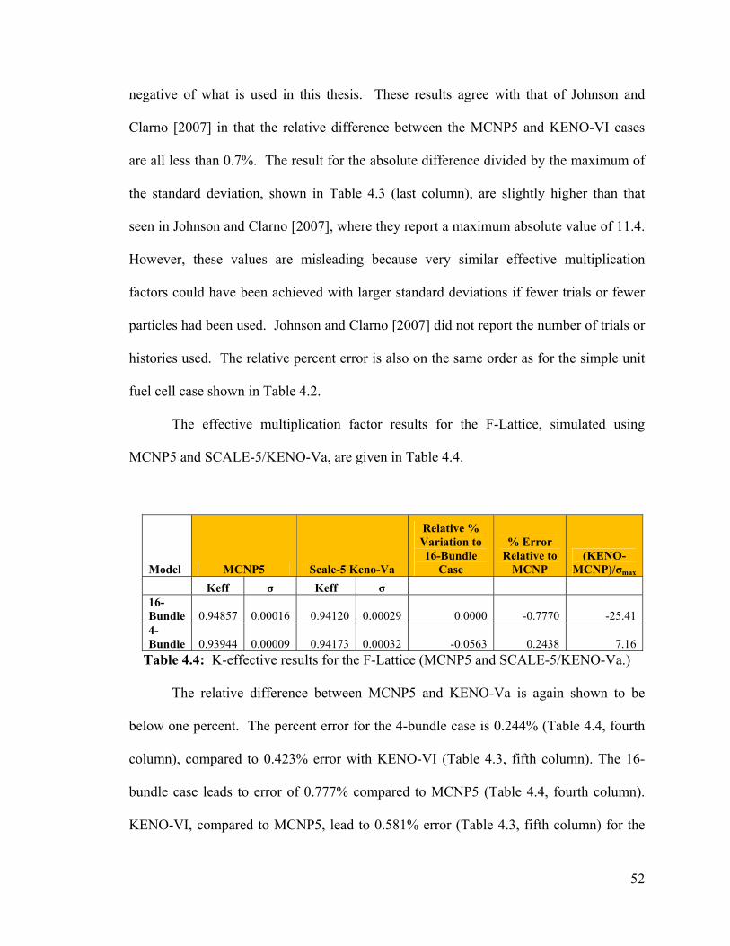
52
negative of what is used in this thesis. These results agree with that of Johnson and
Clarno [2007] in that the relative difference between the MCNP5 and KENO-VI cases
are all less than 0.7%. The result for the absolute difference divided by the maximum of
the standard deviation, shown in Table 4.3 (last column), are slightly higher than that
seen in Johnson and Clarno [2007], where they report a maximum absolute value of 11.4.
However, these values are misleading because very similar effective multiplication
factors could have been achieved with larger standard deviations if fewer trials or fewer
particles had been used. Johnson and Clarno [2007] did not report the number of trials or
histories used. The relative percent error is also on the same order as for the simple unit
fuel cell case shown in Table 4.2.
The effective multiplication factor results for the F-Lattice, simulated using
MCNP5 and SCALE-5/KENO-Va, are given in Table 4.4.
Model MCNP5 Scale-5 Keno-Va
Relative % Variation to 16-Bundle
Case
% Error Relative to
MCNP (KENO-
MCNP)/σmax Keff σ Keff σ 16-Bundle 0.94857 0.00016 0.94120 0.00029 0.0000 -0.7770 -25.41 4-Bundle 0.93944 0.00009 0.94173 0.00032 -0.0563 0.2438 7.16
Table 4.4: K-effective results for the F-Lattice (MCNP5 and SCALE-5/KENO-Va.)
The relative difference between MCNP5 and KENO-Va is again shown to be
below one percent. The percent error for the 4-bundle case is 0.244% (Table 4.4, fourth
column), compared to 0.423% error with KENO-VI (Table 4.3, fifth column). The 16-
bundle case leads to error of 0.777% compared to MCNP5 (Table 4.4, fourth column).
KENO-VI, compared to MCNP5, lead to 0.581% error (Table 4.3, fifth column) for the
53
16-bundle case. The absolute difference over the maximum standard deviation is rather
large for the 16-Bundle case at -25.41. However, this value for the 4-bundle case (7.16)
is within an acceptable range of variation between MCNP5 and SCALE-5 KENO-Va.
Results of the flux analysis for the 4-bundle model are presented below.
Flux calculations were performed for the 4-bundle case using the F4 tally in
MCNP5, and in KENO-Va using the MFX and MSH options located under the
TSUNAMI-3D Parameters tab, which is a subset of ‘Parameter Data’ only found in
SCALE-5. As discussed in Section 4.5 and Section 3.3, only cubic meshes that have
equal spacing in all directions can be defined in SCALE-5. This results in very large
output files, taxing available memory and hard drive space. Thus, the meshes studied (10
cm, 5 cm and 3cm) are rather coarse for the system. Memory limitations are also the
reason as to why the 4-bundle case was used and not the larger 16-bundle system.
Additionally, SCALE-5 produces different results depending on how the Global Unit is
defined, where the Global Unit is the final (largest) geometric unit that contains all other
units and where the boundary conditions are applied. The Global Unit can be defined as
an array or it can be defined as a cuboid that is of the same size as the array and contains
that array. The results for the array-defined Global Unit are given in Table 4.5, and the
results for the cuboid-defined Global Unit are included in Table 4.6. Reported values for
k-effective and flux calculations vary depending on which type of Global Unit is used.
This is an effect of how the initial calculations are performed for the volume weighted
averaging integrals that SCALE uses for its calculations [SCALE: A Modular Code
2006]. The cuboid-defined Global Unit case leads to more accurate results when
compared to the MCNP5 results than the array-defined Global Unit case and thus, is the
54
focus of discussion in this thesis. The k-effective results in Table 4.4 are from the
cuboid-defined Global Unit. Simulations using the array-defined Global Unit produced a
k-effective of 0.94267 with a standard deviation of 0.00028 for the 4-bundle case.
Compared to MCNP5 benchmark results, this is a 0.344% error, whereas the cuboid-
defined Global Unit had a smaller error of 0.244%. In Table 4.5 and Table 4.6 the
location of the peak flux value is given; the origin (0, 0, 0) is defined at the bottom left
corner, and z = 0, of the 4-bundle cell shown in Figure 4.4.
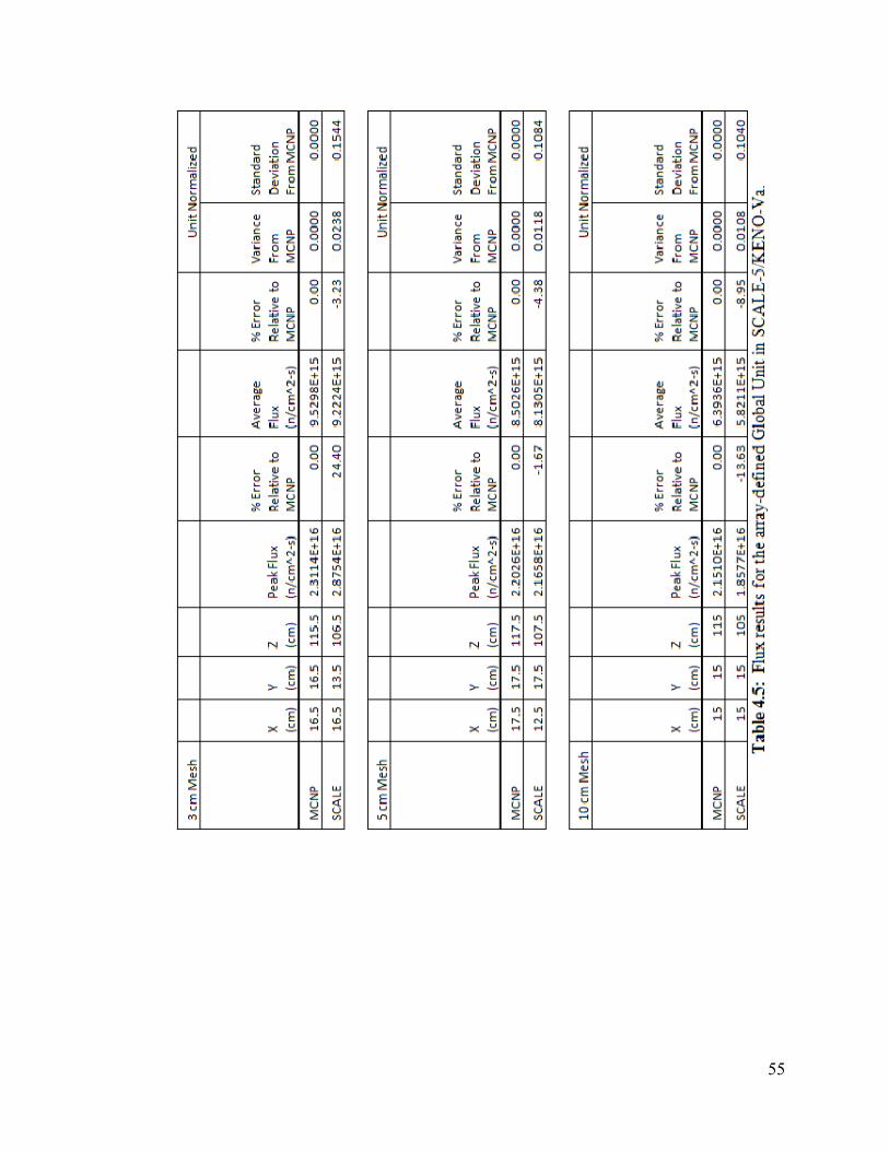
55
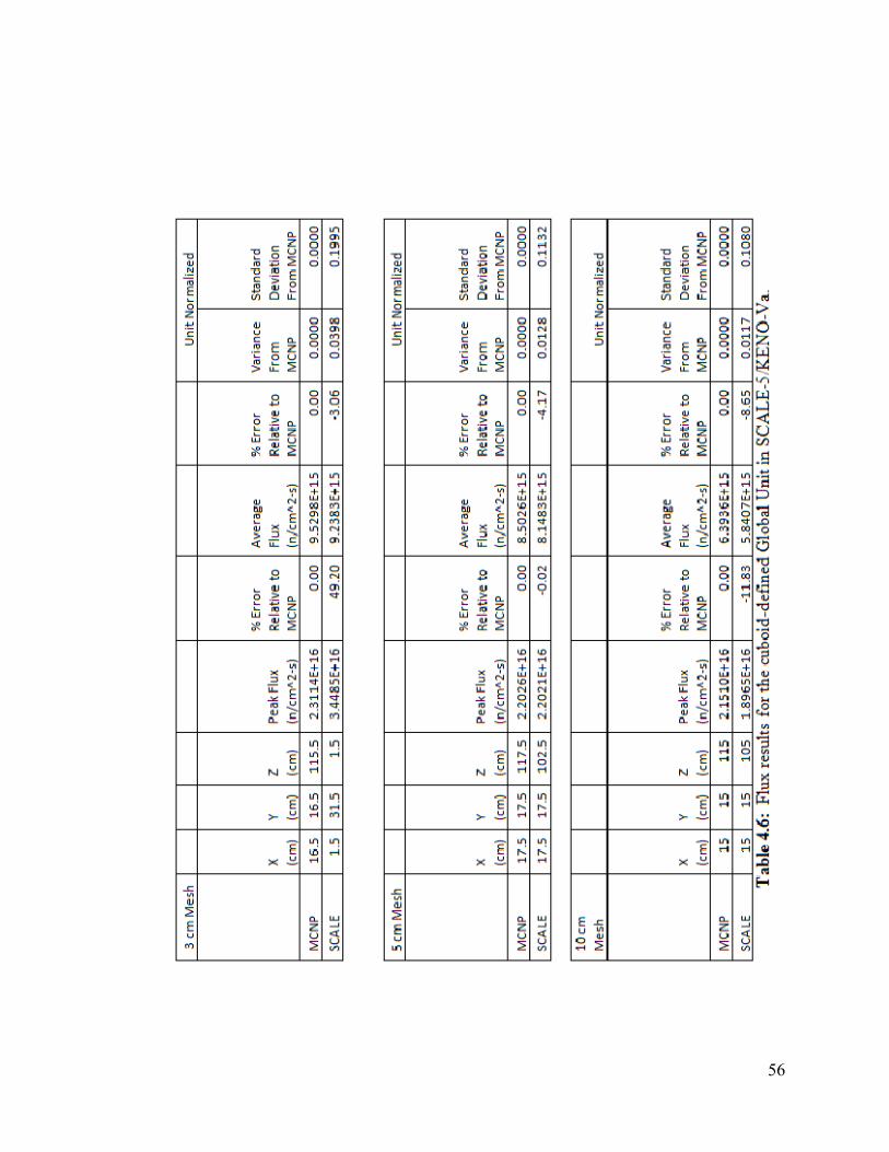
56
57
Flux distributions were synthesized from the SCALE-5/KENO-Va output using
the FluxParse.pl script discussed in Section 4.5, and scaled to real flux values using
Equation 4.1. The SCALE-5/KENO-Va average flux values are within close agreement
with the MCNP5 results. The 3 cm mesh produced the smallest error at 3.06%, followed
by the 5 cm mesh with 4.17% and the 10 cm mesh with 8.65%. As the mesh is refined
further, it is very likely that the results will agree even better with those obtained using
MCNP5; however, due to memory limitations, further refinement was not carried out.
The error in peak flux results showed an unexpectedly large error for the 3 cm
mesh. The 3 cm mesh lead to a 49.20% difference for the SCALE-5/KENO-Va results
compared to the MCNP5 results, whereas the 5 cm mesh only differed by 0.02% (Table
4.6, fifth column). Additionally, as shown in Table 4.6, the difference in peak flux
location is rather significant for the 3 cm mesh. To explore the discrepancy in these
results, three-dimensional contour plots for MCNP5 and SCALE-5 are shown in Figure
4.7 – Figure 4.10.
Figure 4.7 and Figure 4.8 are the xy-plane surface contour plots for z = 115.5 cm,
the location of the MCNP5 peak flux value of 2.3114e+16 neutrons per centimeter
squared per second. Figure 4.9 and Figure 4.10 are the xy-plane surface contour plots for
z = 1.5 cm, the location of the SCALE-5 peak flux value of 3.4485e+16 neutrons per
centimeter squared per second. SCALE-5 results in less smooth contour plot for both
Figure 4.8 and Figure 4.10. This is a result of some of the approximations discussed in
Chapter 2, the difference in approaches that each code system uses and also probably
more importantly, the volume averaging error mentioned in Section 4.3 which is
introduced in scaling the flux values to the same units as the MCNP5 values.
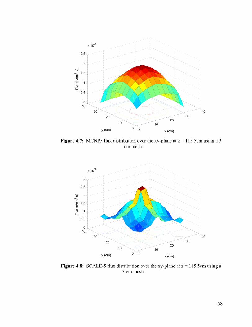
58
010
2030
40
010
20
30400
0.5
1
1.5
2
2.5
x 1016
x (cm)y (cm)
Flux
(n/c
m2 -s
)
Figure 4.7: MCNP5 flux distribution over the xy-plane at z = 115.5cm using a 3
cm mesh.
010
2030
40
010
20
30400
0.5
1
1.5
2
2.5
3
x 1016
x (cm)y (cm)
Flux
(n/c
m2 -s
)
Figure 4.8: SCALE-5 flux distribution over the xy-plane at z = 115.5cm using a
3 cm mesh.
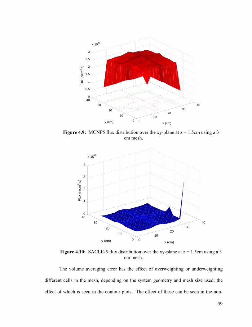
59
010
2030
40
010
20
30400
0.5
1
1.5
2
2.5
3
x 1015
x (cm)y (cm)
Flux
(n/c
m2 -s
)
Figure 4.9: MCNP5 flux distribution over the xy-plane at z = 1.5cm using a 3
cm mesh.
010
2030
40
010
20
30400
1
2
3
4
x 1016
x (cm)y (cm)
Flux
(n/c
m2 -s
)
Figure 4.10: SACLE-5 flux distribution over the xy-plane at z = 1.5cm using a 3
cm mesh.
The volume averaging error has the effect of overweighting or underweighting
different cells in the mesh, depending on the system geometry and mesh size used; the
effect of which is seen in the contour plots. The effect of these can be seen in the non-
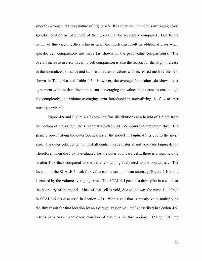
60
smooth (wrong curvature) nature of Figure 4.8. It is clear that due to this averaging error,
specific location or magnitude of the flux cannot be accurately compared. Due to the
nature of this error, further refinement of the mesh can result in additional error when
specific cell comparisons are made (as shown by the peak value comparisons). The
overall increase in error in cell to cell comparison is also the reason for the slight increase
in the normalized variance and standard deviation values with increased mesh refinement
shown in Table 4.6 and Table 4.5. However, the average flux values do show better
agreement with mesh refinement because averaging the values helps cancels out, though
not completely, the volume averaging error introduced in normalizing the flux to “per
starting particle”.
Figure 4.9 and Figure 4.10 show the flux distributions at a height of 1.5 cm from
the bottom of the system, the z plane at which SCALE-5 shows the maximum flux. The
sharp drop-off along the outer boundaries of the model in Figure 4.9 is due to the mesh
size. The outer cells contain almost all control blade material and void (see Figure 4.11).
Therefore, when the flux is evaluated for the outer boundary cells, there is a significantly
smaller flux than compared to the cells (containing fuel) next to the boundaries. The
location of the SCALE-5 peak flux value can be seen to be an anomaly (Figure 4.10), and
is caused by the volume averaging error. The SCALE-5 peak is a data spike in a cell near
the boundary of the model. Most of that cell is void, due to the way the mesh is defined
in SCALE-5 (as discussed in Section 4.3). With a cell that is mostly void, multiplying
the flux result for that location by an average “region volume” (described in Section 4.5)
results in a very large overestimation of the flux in that region. Taking this into
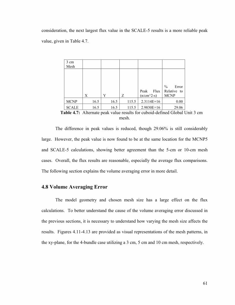
61
consideration, the next largest flux value in the SCALE-5 results is a more reliable peak
value, given in Table 4.7.
3 cm Mesh
X Y Z Peak Flux (n/cm^2-s)
% Error Relative to MCNP
MCNP 16.5 16.5 115.5 2.3114E+16 0.00 SCALE 16.5 16.5 115.5 2.9830E+16 29.06
Table 4.7: Alternate peak value results for cuboid-defined Global Unit 3 cm mesh.
The difference in peak values is reduced, though 29.06% is still considerably
large. However, the peak value is now found to be at the same location for the MCNP5
and SCALE-5 calculations, showing better agreement than the 5-cm or 10-cm mesh
cases. Overall, the flux results are reasonable, especially the average flux comparisons.
The following section explains the volume averaging error in more detail.
4.8 Volume Averaging Error
The model geometry and chosen mesh size has a large effect on the flux
calculations. To better understand the cause of the volume averaging error discussed in
the previous sections, it is necessary to understand how varying the mesh size affects the
results. Figures 4.11-4.13 are provided as visual representations of the mesh patterns, in
the xy-plane, for the 4-bundle case utilizing a 3 cm, 5 cm and 10 cm mesh, respectively.
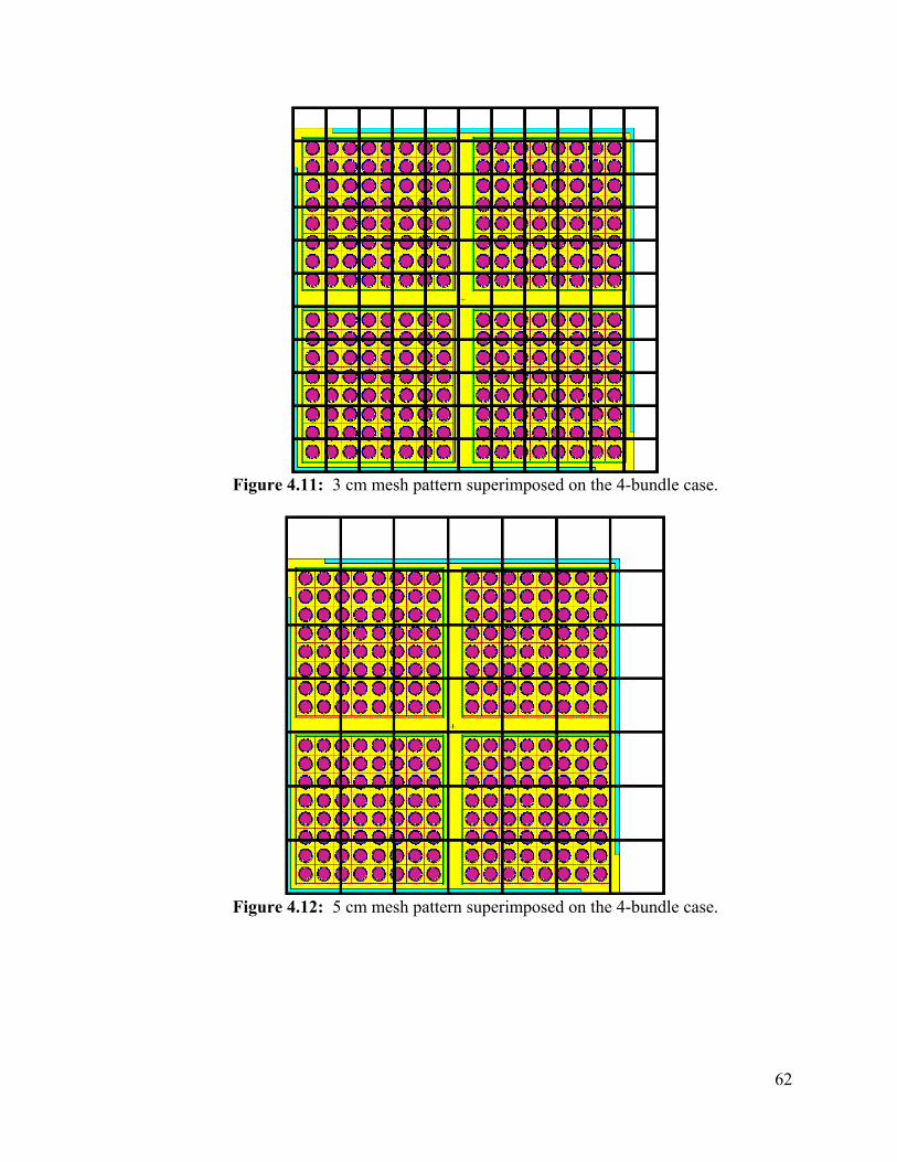
62
Figure 4.11: 3 cm mesh pattern superimposed on the 4-bundle case.
Figure 4.12: 5 cm mesh pattern superimposed on the 4-bundle case.
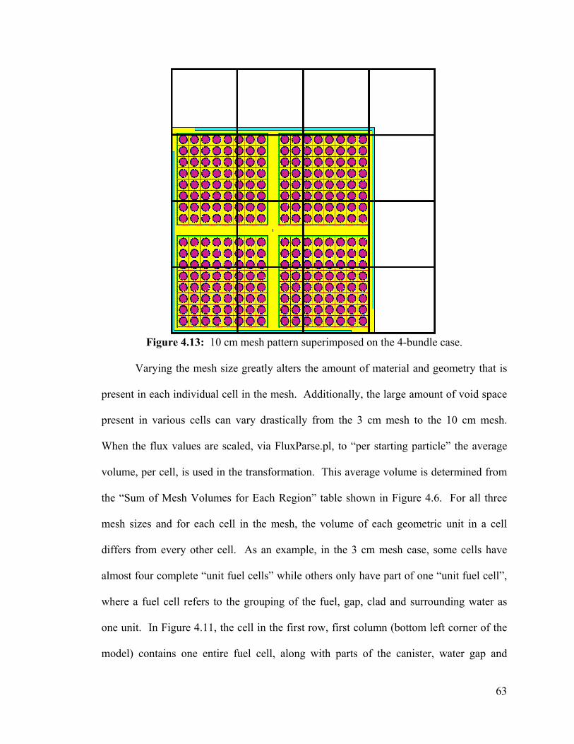
63
Figure 4.13: 10 cm mesh pattern superimposed on the 4-bundle case.
Varying the mesh size greatly alters the amount of material and geometry that is
present in each individual cell in the mesh. Additionally, the large amount of void space
present in various cells can vary drastically from the 3 cm mesh to the 10 cm mesh.
When the flux values are scaled, via FluxParse.pl, to “per starting particle” the average
volume, per cell, is used in the transformation. This average volume is determined from
the “Sum of Mesh Volumes for Each Region” table shown in Figure 4.6. For all three
mesh sizes and for each cell in the mesh, the volume of each geometric unit in a cell
differs from every other cell. As an example, in the 3 cm mesh case, some cells have
almost four complete “unit fuel cells” while others only have part of one “unit fuel cell”,
where a fuel cell refers to the grouping of the fuel, gap, clad and surrounding water as
one unit. In Figure 4.11, the cell in the first row, first column (bottom left corner of the
model) contains one entire fuel cell, along with parts of the canister, water gap and
64
control blade. The cell in second row, second column contains parts of four different
“unit fuel cells”. Considering just the fuel for this example, there is approximately a
factor of four more fuel present in the second row, second column cell than there is in the
first row, first column cell. However, the volume averaging technique in FluxParse.pl
assumes that if fuel is present in any cell, the fuel volume in the cell is equal to the total
volume of fuel in the model divided by the number of cells (the average volume). Each
cell clearly contains a different volume of fuel (and other materials). The use of an
average volume for all cells results in the large difference when specific cell values are
directly compared to MCNP5 results. (FluxParse.pl multiplies all flux values by the
volume of the geometric unit present in the cell for which the flux is reported. This is
done to transfrom the flux normalization from “per unit volume per starting particle” to
“per starting particle”. See Section 4.5) Calculating “region volumes” that are not
averaged cannot be automated, as discussed in Section 4.5. Therefore, manual
calculation of the volume of each geometric unit within specific cells is required to
eliminate the volume averaging error.
To determine how large an effect the volume averaging has on the flux
calculations, it is necessary to perform manual “region volume” calculations for specific
cells. As mentioned in Section 4.3, this would be extremely difficult and very intensive
due to the fact that each cell requires unique “region volume” calculations. Therefore,
only the cells of the peak flux values determined by MCNP5 (as reported in Table 4.6)
are explored in greater detail here. Figure 4.14, Figure 4.15 and Figure 4.16 are enlarged
views of the cells being analyzed.
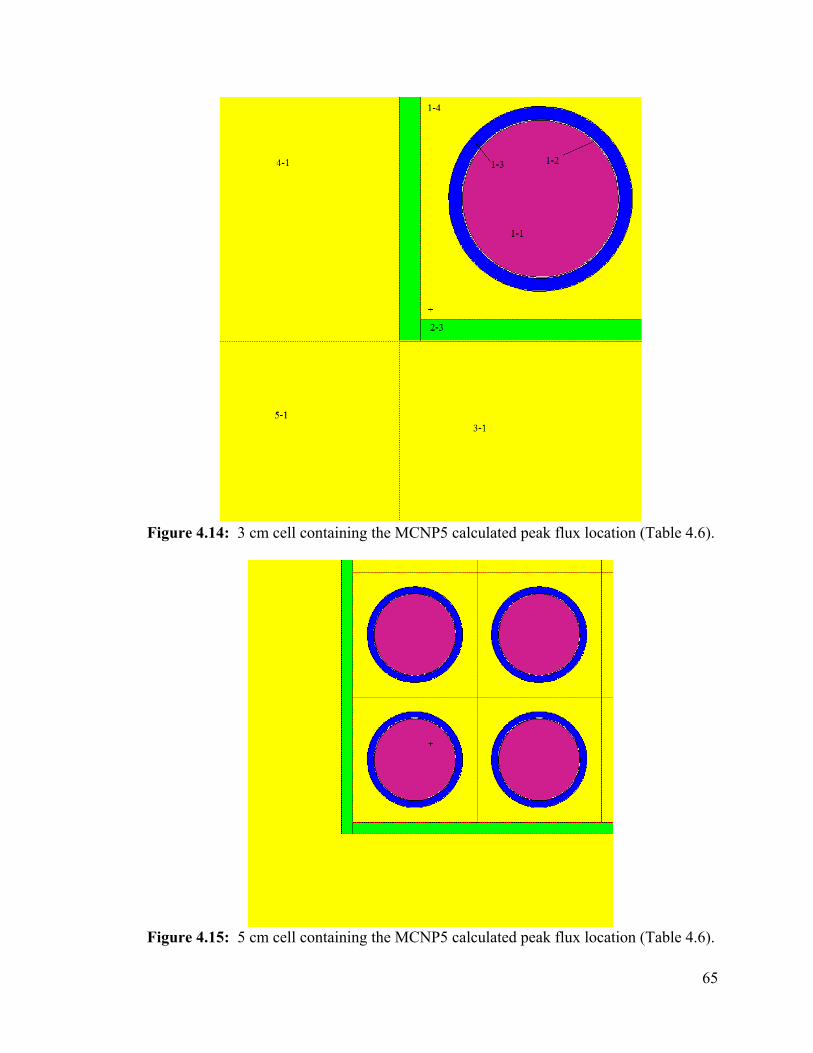
65
Figure 4.14: 3 cm cell containing the MCNP5 calculated peak flux location (Table 4.6).
Figure 4.15: 5 cm cell containing the MCNP5 calculated peak flux location (Table 4.6).
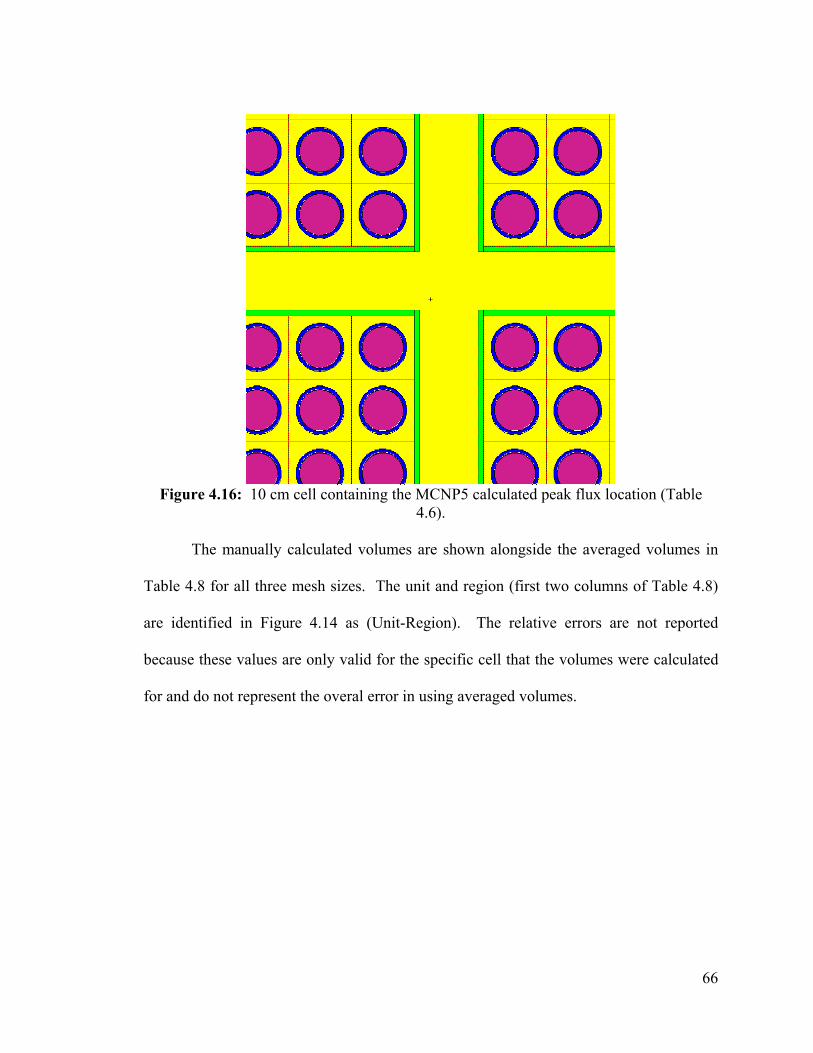
66
Figure 4.16: 10 cm cell containing the MCNP5 calculated peak flux location (Table
4.6).
The manually calculated volumes are shown alongside the averaged volumes in
Table 4.8 for all three mesh sizes. The unit and region (first two columns of Table 4.8)
are identified in Figure 4.14 as (Unit-Region). The relative errors are not reported
because these values are only valid for the specific cell that the volumes were calculated
for and do not represent the overal error in using averaged volumes.
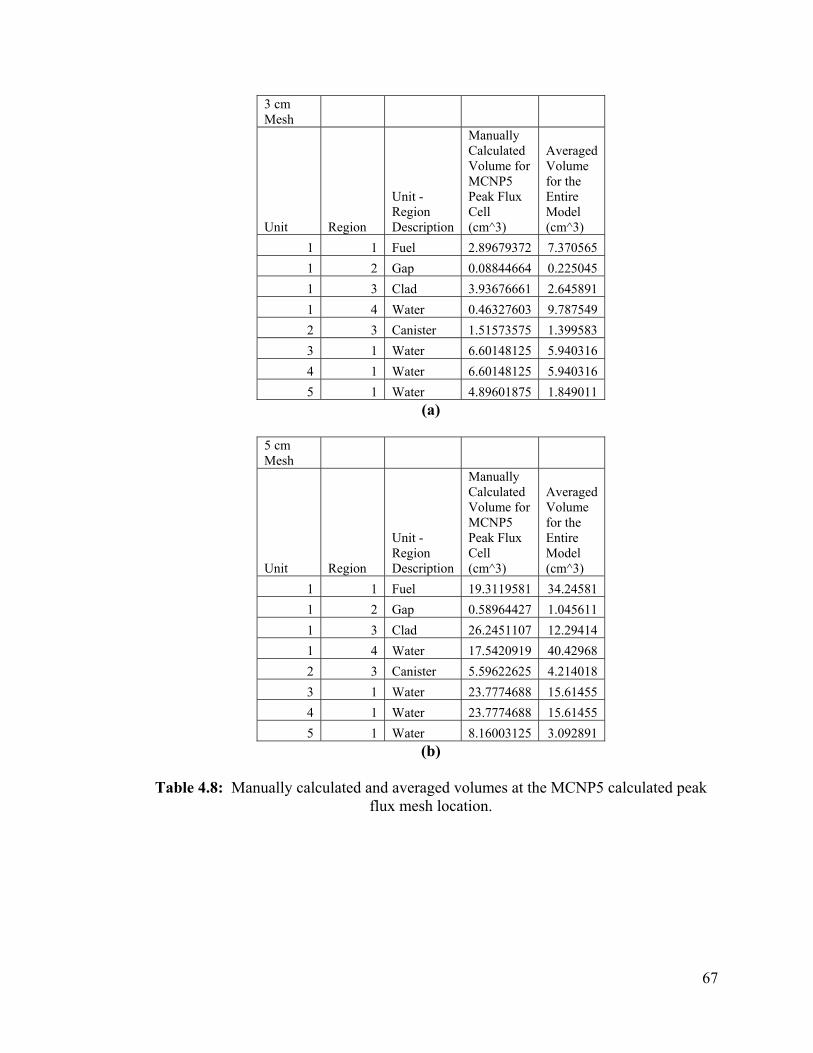
67
3 cm Mesh
Unit Region
Unit - Region Description
Manually Calculated Volume for MCNP5 Peak Flux Cell (cm^3)
Averaged Volume for the Entire Model (cm^3)
1 1 Fuel 2.89679372 7.370565 1 2 Gap 0.08844664 0.225045 1 3 Clad 3.93676661 2.645891 1 4 Water 0.46327603 9.787549 2 3 Canister 1.51573575 1.399583 3 1 Water 6.60148125 5.940316 4 1 Water 6.60148125 5.940316 5 1 Water 4.89601875 1.849011
(a)
5 cm Mesh
Unit Region
Unit - Region Description
Manually Calculated Volume for MCNP5 Peak Flux Cell (cm^3)
Averaged Volume for the Entire Model (cm^3)
1 1 Fuel 19.3119581 34.24581 1 2 Gap 0.58964427 1.045611 1 3 Clad 26.2451107 12.29414 1 4 Water 17.5420919 40.42968 2 3 Canister 5.59622625 4.214018 3 1 Water 23.7774688 15.61455 4 1 Water 23.7774688 15.61455 5 1 Water 8.16003125 3.092891
(b)
Table 4.8: Manually calculated and averaged volumes at the MCNP5 calculated peak flux mesh location.
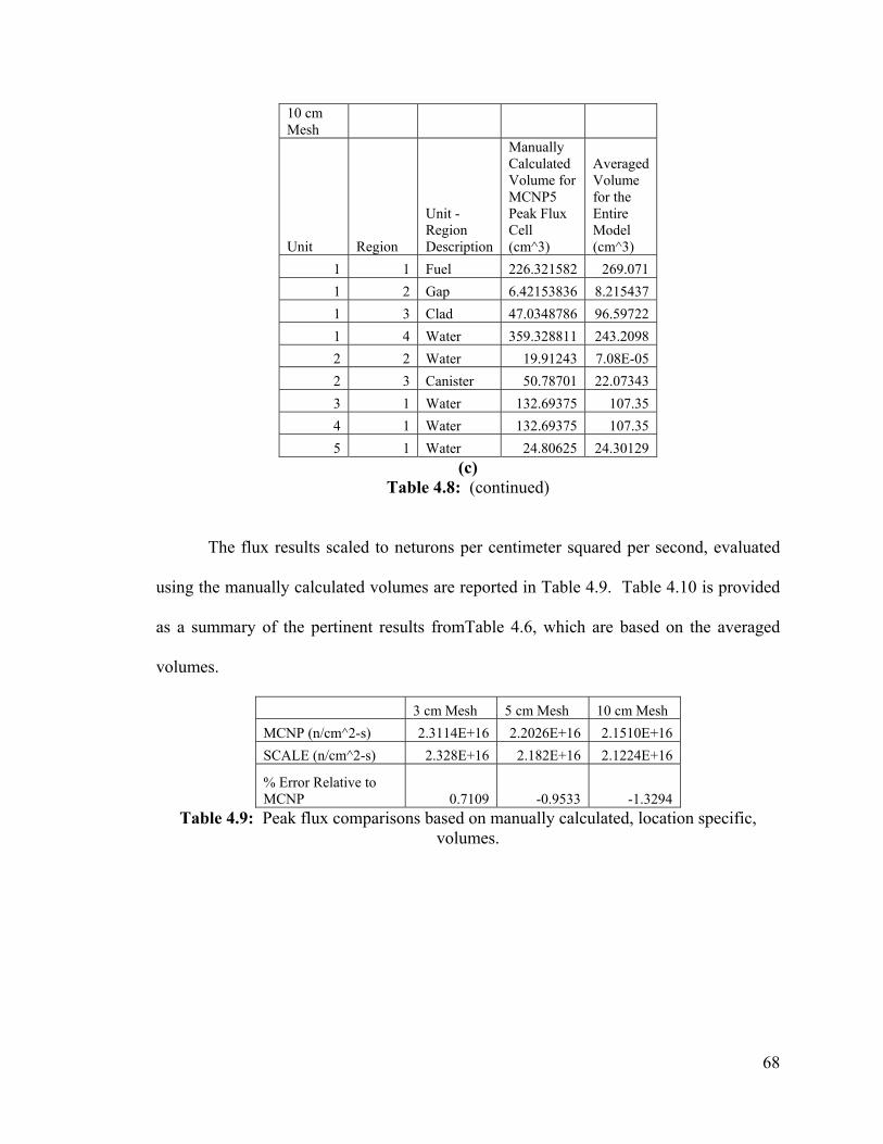
68
10 cm Mesh
Unit Region
Unit - Region Description
Manually Calculated Volume for MCNP5 Peak Flux Cell (cm^3)
Averaged Volume for the Entire Model (cm^3)
1 1 Fuel 226.321582 269.071 1 2 Gap 6.42153836 8.215437 1 3 Clad 47.0348786 96.59722 1 4 Water 359.328811 243.2098 2 2 Water 19.91243 7.08E-05 2 3 Canister 50.78701 22.07343 3 1 Water 132.69375 107.35 4 1 Water 132.69375 107.35 5 1 Water 24.80625 24.30129
(c) Table 4.8: (continued)
The flux results scaled to neturons per centimeter squared per second, evaluated
using the manually calculated volumes are reported in Table 4.9. Table 4.10 is provided
as a summary of the pertinent results fromTable 4.6, which are based on the averaged
volumes.
3 cm Mesh 5 cm Mesh 10 cm Mesh MCNP (n/cm^2-s) 2.3114E+16 2.2026E+16 2.1510E+16 SCALE (n/cm^2-s) 2.328E+16 2.182E+16 2.1224E+16
% Error Relative to MCNP 0.7109 -0.9533 -1.3294
Table 4.9: Peak flux comparisons based on manually calculated, location specific, volumes.
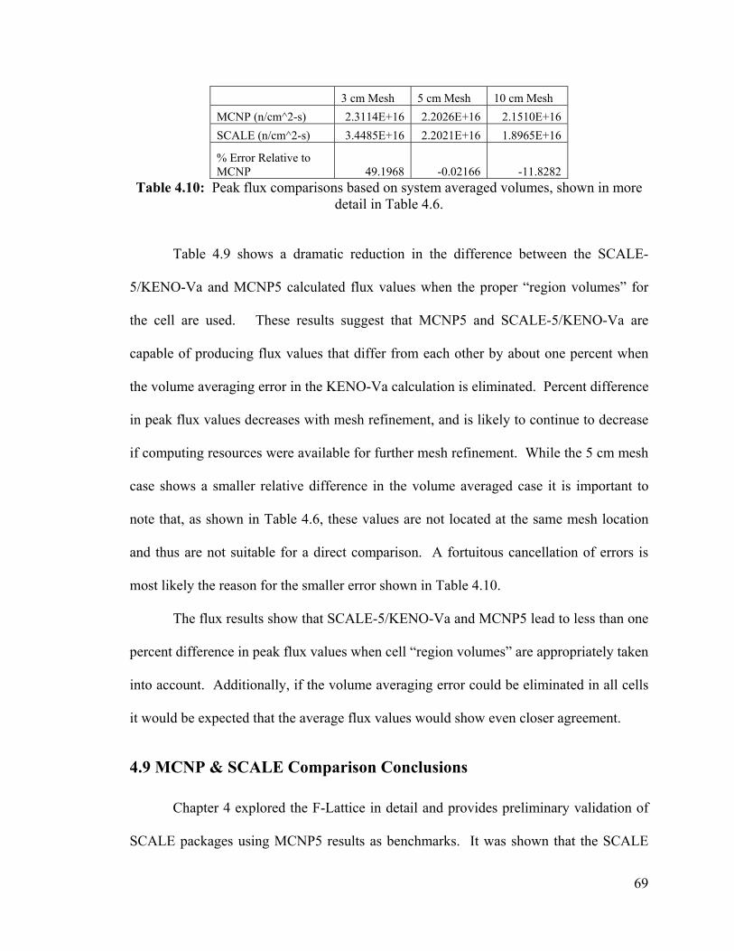
69
3 cm Mesh 5 cm Mesh 10 cm Mesh MCNP (n/cm^2-s) 2.3114E+16 2.2026E+16 2.1510E+16 SCALE (n/cm^2-s) 3.4485E+16 2.2021E+16 1.8965E+16
% Error Relative to MCNP 49.1968 -0.02166 -11.8282
Table 4.10: Peak flux comparisons based on system averaged volumes, shown in more detail in Table 4.6.
Table 4.9 shows a dramatic reduction in the difference between the SCALE-
5/KENO-Va and MCNP5 calculated flux values when the proper “region volumes” for
the cell are used. These results suggest that MCNP5 and SCALE-5/KENO-Va are
capable of producing flux values that differ from each other by about one percent when
the volume averaging error in the KENO-Va calculation is eliminated. Percent difference
in peak flux values decreases with mesh refinement, and is likely to continue to decrease
if computing resources were available for further mesh refinement. While the 5 cm mesh
case shows a smaller relative difference in the volume averaged case it is important to
note that, as shown in Table 4.6, these values are not located at the same mesh location
and thus are not suitable for a direct comparison. A fortuitous cancellation of errors is
most likely the reason for the smaller error shown in Table 4.10.
The flux results show that SCALE-5/KENO-Va and MCNP5 lead to less than one
percent difference in peak flux values when cell “region volumes” are appropriately taken
into account. Additionally, if the volume averaging error could be eliminated in all cells
it would be expected that the average flux values would show even closer agreement.
4.9 MCNP & SCALE Comparison Conclusions
Chapter 4 explored the F-Lattice in detail and provides preliminary validation of
SCALE packages using MCNP5 results as benchmarks. It was shown that the SCALE
70
results, both for SCALE-5.1/KENO-VI and SCALE-5/KENO-Va, are within one percent
of the MCNP5 results. This is in agreement with the work reported by Johnson and
Clarno [2007]. However, since SCALE-5/KENO-Va provides accurate results, allows
for a superimposed mesh for flux calculations and is less computationally intensive than
SCALE-5.1, SCALE-5.1/KENO-VI can be quickly ruled out for use for the F-Lattice.
Additionally, this chapter explored SCALE-5/KENO-Va to report flux
distributions; a use not found in literature. A Perl script was written to extract the large
and “disorganized” flux values from the SCALE-5 output files. The Perl script was
written so that it can be used with any arbitrary system or mesh size. Average flux values
were shown to be highly accurate, within 3.06%, and would most likely improve in
accuracy as the mesh is further refined. Specific values however cannot be trusted with
complete accuracy due to a volume averaging error in normalizing the SCALE-5 flux
values to “per starting particle.” The effect of the volume averaging error on the flux
calculations was quantified in Section 4.8. An approach to eliminate this error is
discussed in Section 6.2: Future Work.
Having developed the tools, and then using them to compare flux values and
validating their results, along with more general k-effective calculations, SCALE-
5/KENO-Va is considered reliable for modeling the F-Lattice. SCALE-5 is compared
with MCNP5 for some parametric studies of the F-Lattice in the next chapter. Rod worth
calculations are performed for the F-Lattice control blades. Additionally, MCNP5 is used
more extensively to analyze the effects that geometry and material changes have on the
neutron flux profiles of the system.
71
Chapter 5: Parametric Studies
The effects of varying material properties and geometry within the F-Lattice are
investigated in this chapter. The effective rod worth of the standard B4C control blades is
determined by comparing reactivity change when B4C is replaced by pure graphite
blades. Geometric effects on rod worth are also investigated by varying the thickness of
the control blades. Thickness changes affect rod worth directly in terms of volume of
control material present, as well as a slight effect on the control blade surface area.
Additionally, the water moderator gap is altered by changes in control blade thickness
because pitch is kept constant. The changes in the effective multiplication factor, as well
as pertinent neutron flux values, are studied using both MCNP5 and SCALE-5/KENO-Va
to assess the capabilities of KENO-Va to model the variations in the F-Lattice.
Additionally, neutron flux profiles are analyzed for each case by MCNP5.
5.1 Material Change: Graphite
The key feature of the F-Lattice is the increased width of the control blades and
the staggered row configuration. The nominal case of B4C control rods with a thickness
of 8.3 mm was analyzed in Section 4.7. The rod worth of the F-Lattice control blades is
studied by replacing the blades by a moderator. The B4C control rods are replaced by
pure graphite. Graphite, or carbon, primarily scatters neutrons while Boron, present in
B4C, acts as a strong absorber [Duderstadt and Hamilton 1976]. Therefore, the control
(absorption) material has been completely removed and replaced by a moderating
material. In terms of rod worth, this represents an instantaneous reactivity change. Rod
worth is evaluated as [Lamarsh 1966]:
72
kkk o
w−
=ρ (5.1)
Where ko is the multiplication factor with control rods inserted in, and k is the
multiplication factor with the control rods pulled out and replaced with pure graphite.
When B4C is replaced by graphite, neutron absorption dramatically decreases, causing an
increase in neutron population, increase in flux and a larger effective multiplication
factor. (Standard rod worth analysis is performed by replacing the control rods with the
system’s moderator material, which is light water for the F-Lattice. However, rod worth
is determined by replacing B4C with graphite to additionally study the effect of a
significant material change.) The results of SCALE-5/KENO-Va, compared to the
benchmark MCNP5 results, are presented in the following section to quantify the effect
of this material change.
5.2 Material Change Results: Rod Worth
The SCALE-5/KENO-Va simulations were run for both the 4-bundle case and the
16-bundle case with 10,000 particles for 250 inactive cycles and 550 active cycles.
MCNP5 simulations were carried out with 50,000 particles for 250 inactive cycles and
350 active cycles for the 16-bundle case. The MCNP5 4-bundle case used 100,000
particles for 250 inactive cycles and 550 active cycles. The 4-bundle case was run with
more particles and histories to ensure accurate flux results. It is not necessary to run the
16-bundle case, which has a very large computational cost, for higher accuracy because
results from the 4-bundle and 16-bundle case differ negligibly. The resulting effective
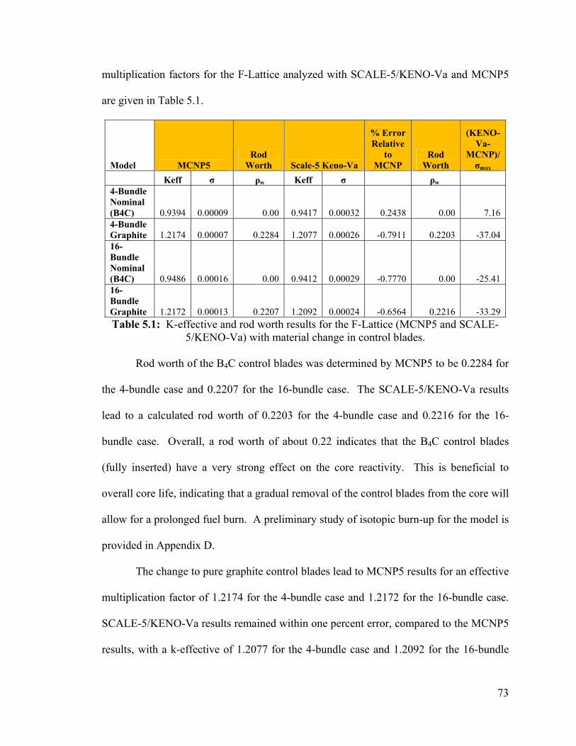
73
multiplication factors for the F-Lattice analyzed with SCALE-5/KENO-Va and MCNP5
are given in Table 5.1.
Model MCNP5 Rod
Worth Scale-5 Keno-Va
% Error Relative
to MCNP
Rod Worth
(KENO-Va-
MCNP)/σmax
Keff σ ρw Keff σ ρw 4-Bundle Nominal (B4C) 0.9394 0.00009 0.00 0.9417 0.00032 0.2438 0.00 7.16 4-Bundle Graphite 1.2174 0.00007 0.2284 1.2077 0.00026 -0.7911 0.2203 -37.04 16-Bundle Nominal (B4C) 0.9486 0.00016 0.00 0.9412 0.00029 -0.7770 0.00 -25.41 16-Bundle Graphite 1.2172 0.00013 0.2207 1.2092 0.00024 -0.6564 0.2216 -33.29 Table 5.1: K-effective and rod worth results for the F-Lattice (MCNP5 and SCALE-
5/KENO-Va) with material change in control blades.
Rod worth of the B4C control blades was determined by MCNP5 to be 0.2284 for
the 4-bundle case and 0.2207 for the 16-bundle case. The SCALE-5/KENO-Va results
lead to a calculated rod worth of 0.2203 for the 4-bundle case and 0.2216 for the 16-
bundle case. Overall, a rod worth of about 0.22 indicates that the B4C control blades
(fully inserted) have a very strong effect on the core reactivity. This is beneficial to
overall core life, indicating that a gradual removal of the control blades from the core will
allow for a prolonged fuel burn. A preliminary study of isotopic burn-up for the model is
provided in Appendix D.
The change to pure graphite control blades lead to MCNP5 results for an effective
multiplication factor of 1.2174 for the 4-bundle case and 1.2172 for the 16-bundle case.
SCALE-5/KENO-Va results remained within one percent error, compared to the MCNP5
results, with a k-effective of 1.2077 for the 4-bundle case and 1.2092 for the 16-bundle
74
case. The error is still within the acceptable range of less than one percent and actually
presented a decrease from the nominal 16-bundle case, 0.66% from 0.78%. The absolute
difference, between MCNP5 and SCALE-5/KENO-Va results, divided by the maximum
standard deviations increased, dramatically for the 4-bundle case, when compared to the
nominal B4C case. This can be attributed to the increase, by a factor of three, in the
relative difference, which correlates to a larger absolute difference. The 16-bundle case’s
absolute difference over standard deviation also increased despite a decrease in relative
difference. However, a decrease in relative difference does not necessarily correspond to
a decrease in absolute difference. There is a 28% increase in k-effective for the 16-
bundle case but only an 8% increase in absolute difference, -0.0074 for the nominal B4C
16-bundle case to -0.008 for the graphite 16-bundle case. Additionally, the decrease in
the maximum standard deviation, 0.00024 from 0.00029 in the nominal case, contributes
to an increased absolute difference over maximum standard deviation. While the
absolute difference over the maximum standard deviation is relatively large, the small
relative difference still confirms the results to be accurate for SCALE-5/KENO-Va.
Flux calculations were also compared for the 4-bundle models. The SCALE-5
models used a cuboid-defined Global Unit as it leads to better agreement with MCNP5
results, as discussed in Chapter 4 when compared to the array-defined Global Unit. The
flux results, compared to MCNP5 benchmark results, using a 3 cm mesh, are given in
Table 5.2.
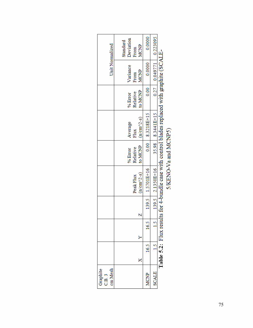
75
76
The average flux values for the two codes are in very close agreement, 0.27%,
which is smaller than the 0.79% difference seen for the k-effective values. Similar to the
flux results in Chapter 4, there is a relatively large difference in peak flux between the
two codes, as well as variation in the location of the peak. However this is again due to
the volume averaging error previously discussed.
Flux profiles were also analyzed on the 16-bundle cases using more advanced
meshing abilities of MCNP5, discussed in Section 4.2. Neutron flux was tracked in the
x-direction with a fine mesh (0.02 cm mesh spacing in the x-direction, with 1 cm mesh
spacing for both the y-direction and z-direction). Due to symmetry, flux profiles in the y-
direction would produce similar results. The flux profile along the x-direction was
analyzed near the middle of the reactor, centered at z = 136.9 cm, and in two different y-
locations for all simulations. These two locations were chosen to monitor the effect the
larger control rods have on neutron population, within the control blade and through a
section of fuel. The first set of flux profiles shown are along a line parallel and through
the center of the main, center control blade present in the 16-bundle case (shown in
Figure 4.3 as line “a”). The second set of flux profiles are along a line that is
perpendicular to, and crosses the main, center control blade. This line is centered through
the midpoint of the fourth fuel cell below the main center control blade, 6.894 cm from
the center of the parallel running control blade (shown in Figure 4.3 as line “b”). The F4
tally was used specifying flux calculation by energy group, as described in Section 4.2.
The energy grouping was 0 - 0.225 eV for thermal neutrons, 0.225 eV – 0.1 MeV for
epithermal neutrons and 0.1 MeV and above for fast neutrons. Total neutron flux was
also evaluated. All flux values are scaled to units of the number of neutrons per

77
centimeter squared per second, as dictated by Equation 4.1, to a power level of 1000
MWt.
Flux calculations that run parallel through the center of the main control blade are
presented first. Thermal neutron flux is shown in Figure 5.1 and provides the most
poignant example of the model’s rod worth. The strong absorber, B4C results in near
zero thermal neutron flux through the center of the control blade. The locations where
the nominal thermal flux dramatically increases correspond to the edges of the control
blades and beginning of the light-water moderator section of the core. The stronger
moderator, graphite, is shown to maintain a high thermal neutron flux throughout the
blade, which is directly related to the significantly larger k-effective associated with the
graphite system.
Figure 5.2 is a plot of the epithermal neutron flux. The graphite system presents a
larger flux profile through the blade than the B4C system. This is expected as more of the
fast neutrons are slowed down via interactions with the graphite than are by B4C. Figure
5.3 provides the flux profile for the fast neutrons. As expected, the graphite system again
presents larger flux values, though it is not as significant as it is in the epithermal or
thermal cases. Slightly more fast neutrons are present in the graphite case due to the
increase in overall fission reactions that are taking place compared to the B4C control rod
system.
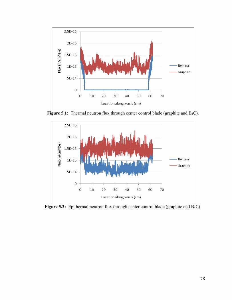
78
Figure 5.1: Thermal neutron flux through center control blade (graphite and B4C).
Figure 5.2: Epithermal neutron flux through center control blade (graphite and B4C).
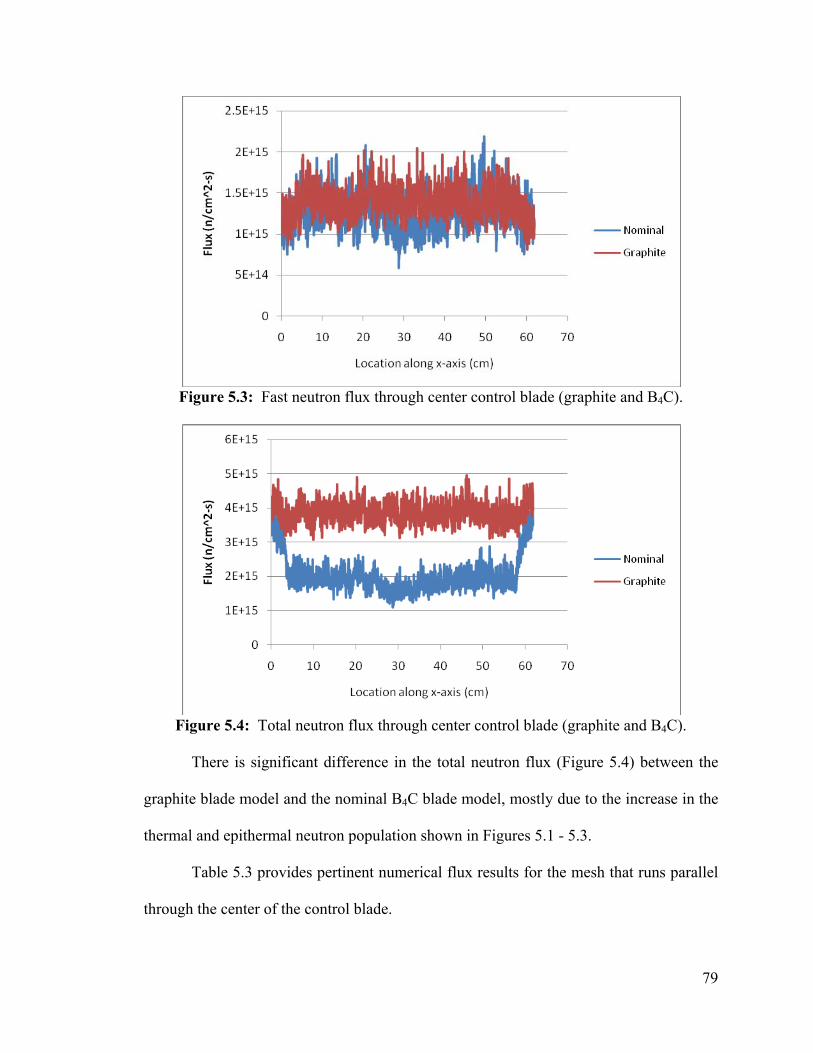
79
Figure 5.3: Fast neutron flux through center control blade (graphite and B4C).
Figure 5.4: Total neutron flux through center control blade (graphite and B4C).
There is significant difference in the total neutron flux (Figure 5.4) between the
graphite blade model and the nominal B4C blade model, mostly due to the increase in the
thermal and epithermal neutron population shown in Figures 5.1 - 5.3.
Table 5.3 provides pertinent numerical flux results for the mesh that runs parallel
through the center of the control blade.
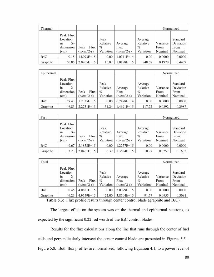
80
Thermal Normalized
Peak Flux Location in X-dimension (cm)
Peak Flux (n/cm^2-s)
Peak Relative % Variation
Average Flux (n/cm^2-s)
Average Relative % Variation
Variance From Nominal
Standard Deviation From Nominal
B4C 0.15 1.8093E+15 0.00 1.0741E+14 0.00 0.0000 0.0000 Graphite 60.85 2.0965E+15 15.87 1.0188E+15 848.58 0.1970 0.4439 Epithermal Normalized
Peak Flux Location in X-dimension (cm)
Peak Flux (n/cm^2-s)
Peak Relative % Variation
Average Flux (n/cm^2-s)
Average Relative % Variation
Variance From Nominal
Standard Deviation From Nominal
B4C 59.43 1.7335E+15 0.00 6.7478E+14 0.00 0.0000 0.0000 Graphite 46.83 2.2751E+15 31.24 1.4691E+15 117.72 0.0892 0.2987 Fast Normalized
Peak Flux Location in X-dimension (cm)
Peak Flux (n/cm^2-s)
Peak Relative % Variation
Average Flux (n/cm^2-s)
Average Relative % Variation
Variance From Nominal
Standard Deviation From Nominal
B4C 49.67 2.1858E+15 0.00 1.2277E+15 0.00 0.0000 0.0000 Graphite 33.23 2.0461E+15 6.39 1.3624E+15 10.97 0.0257 0.1602 Total Normalized
Peak Flux Location in X-dimension (cm)
Peak Flux (n/cm^2-s)
Peak Relative % Variation
Average Flux (n/cm^2-s)
Average Relative % Variation
Variance From Nominal
Standard Deviation From Nominal
B4C 0.45 4.0621E+15 0.00 2.0099E+15 0.00 0.0000 0.0000 Graphite 46.23 4.9559E+15 22.00 3.8504E+15 91.57 0.0955 0.3091
Table 5.3: Flux profile results through center control blade (graphite and B4C).
The largest effect on the system was on the thermal and epithermal neutrons, as
expected by the significant 0.22 rod worth of the B4C control blades.
Results for the flux calculations along the line that runs through the center of fuel
cells and perpendicularly intersect the center control blade are presented in Figures 5.5 –
Figure 5.8. Both flux profiles are normalized, following Equation 4.1, to a power level of
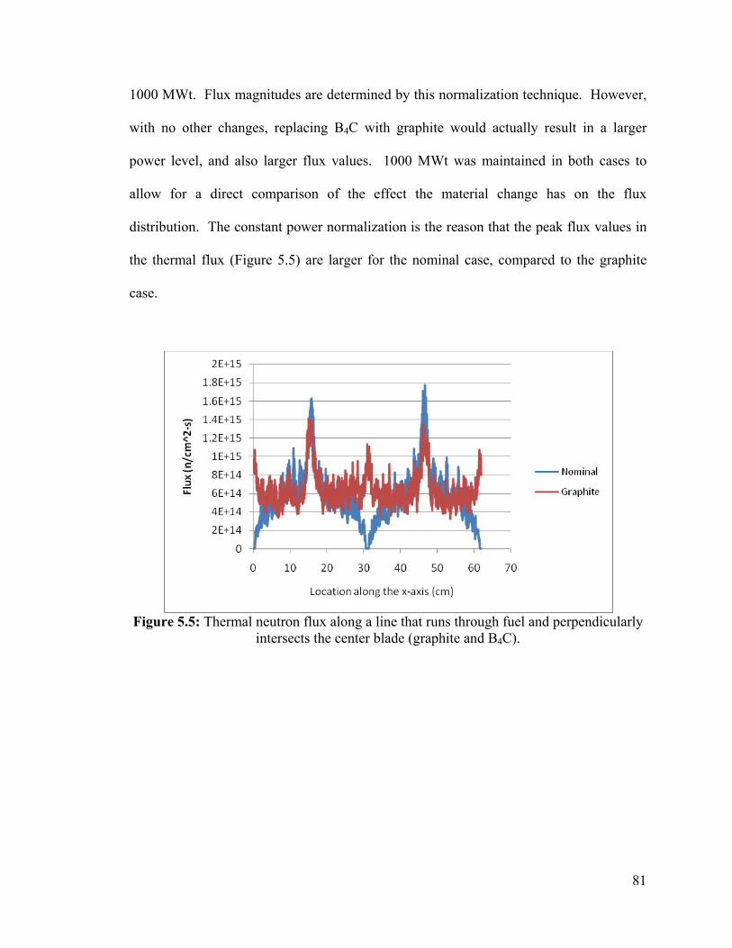
81
1000 MWt. Flux magnitudes are determined by this normalization technique. However,
with no other changes, replacing B4C with graphite would actually result in a larger
power level, and also larger flux values. 1000 MWt was maintained in both cases to
allow for a direct comparison of the effect the material change has on the flux
distribution. The constant power normalization is the reason that the peak flux values in
the thermal flux (Figure 5.5) are larger for the nominal case, compared to the graphite
case.
Figure 5.5: Thermal neutron flux along a line that runs through fuel and perpendicularly
intersects the center blade (graphite and B4C).
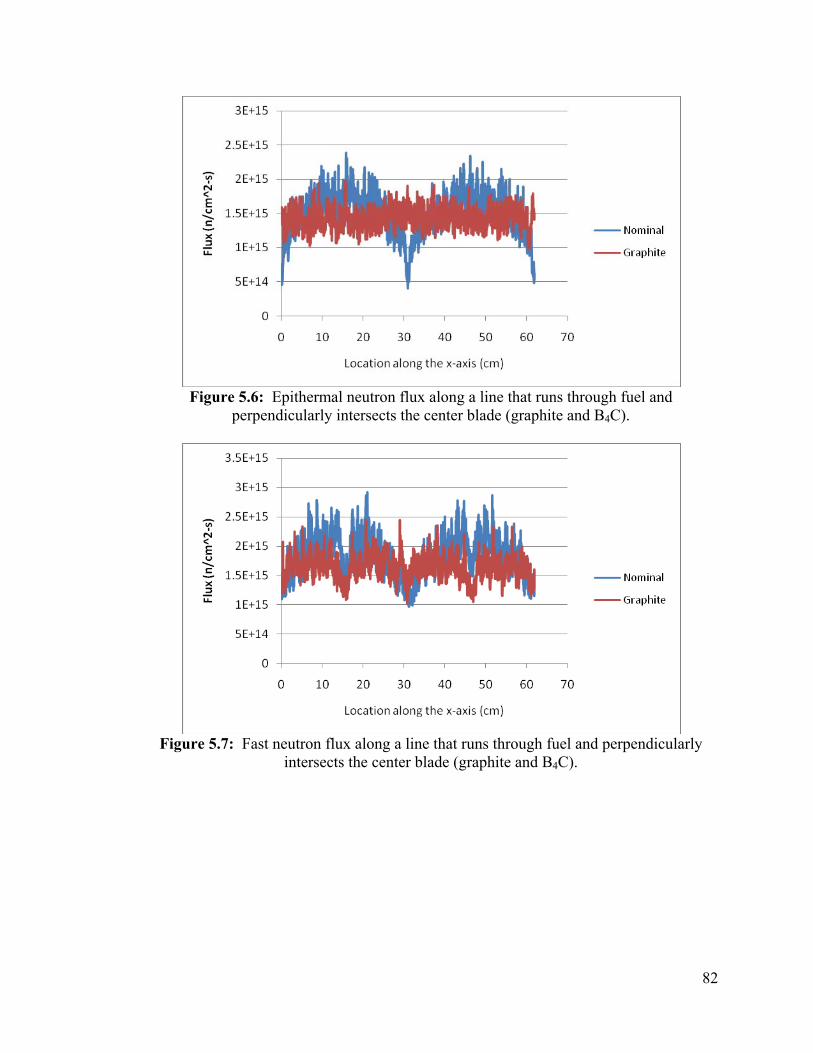
82
Figure 5.6: Epithermal neutron flux along a line that runs through fuel and
perpendicularly intersects the center blade (graphite and B4C).
Figure 5.7: Fast neutron flux along a line that runs through fuel and perpendicularly
intersects the center blade (graphite and B4C).
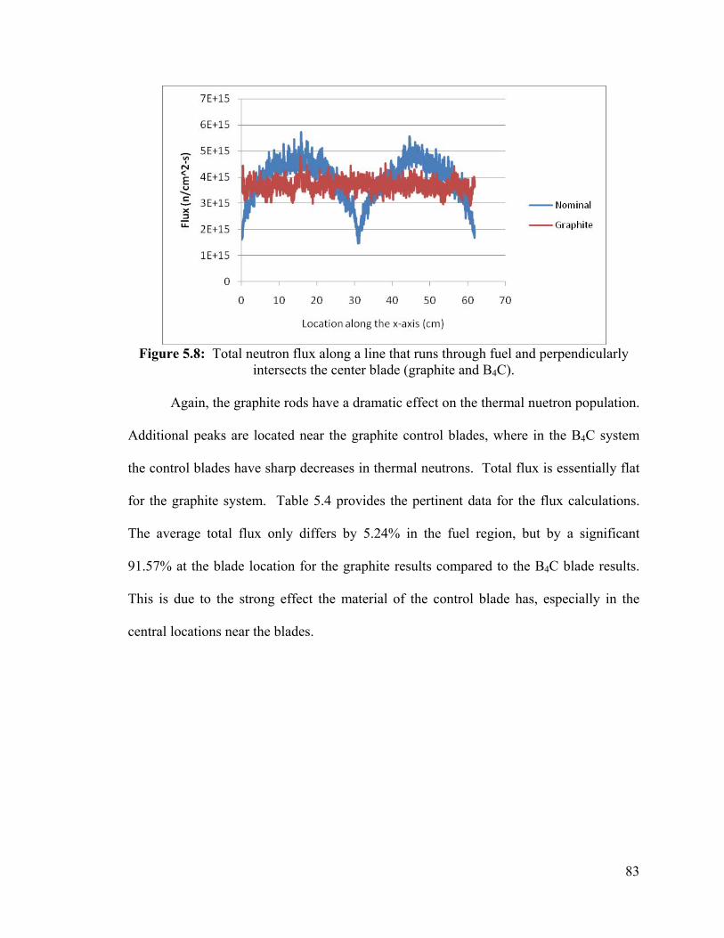
83
Figure 5.8: Total neutron flux along a line that runs through fuel and perpendicularly
intersects the center blade (graphite and B4C). Again, the graphite rods have a dramatic effect on the thermal nuetron population.
Additional peaks are located near the graphite control blades, where in the B4C system
the control blades have sharp decreases in thermal neutrons. Total flux is essentially flat
for the graphite system. Table 5.4 provides the pertinent data for the flux calculations.
The average total flux only differs by 5.24% in the fuel region, but by a significant
91.57% at the blade location for the graphite results compared to the B4C blade results.
This is due to the strong effect the material of the control blade has, especially in the
central locations near the blades.
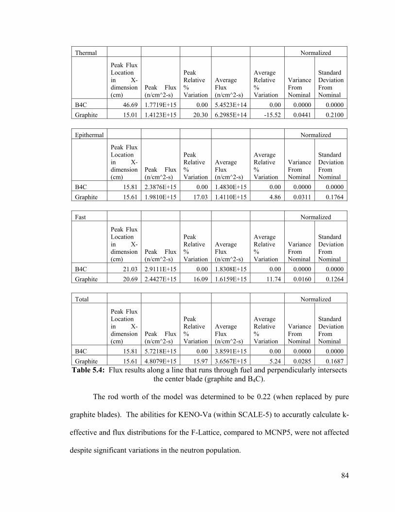
84
Thermal Normalized
Peak Flux Location in X-dimension (cm)
Peak Flux (n/cm^2-s)
Peak Relative % Variation
Average Flux (n/cm^2-s)
Average Relative % Variation
Variance From Nominal
Standard Deviation From Nominal
B4C 46.69 1.7719E+15 0.00 5.4523E+14 0.00 0.0000 0.0000 Graphite 15.01 1.4123E+15 20.30 6.2985E+14 -15.52 0.0441 0.2100 Epithermal Normalized
Peak Flux Location in X-dimension (cm)
Peak Flux (n/cm^2-s)
Peak Relative % Variation
Average Flux (n/cm^2-s)
Average Relative % Variation
Variance From Nominal
Standard Deviation From Nominal
B4C 15.81 2.3876E+15 0.00 1.4830E+15 0.00 0.0000 0.0000 Graphite 15.61 1.9810E+15 17.03 1.4110E+15 4.86 0.0311 0.1764 Fast Normalized
Peak Flux Location in X-dimension (cm)
Peak Flux (n/cm^2-s)
Peak Relative % Variation
Average Flux (n/cm^2-s)
Average Relative % Variation
Variance From Nominal
Standard Deviation From Nominal
B4C 21.03 2.9111E+15 0.00 1.8308E+15 0.00 0.0000 0.0000 Graphite 20.69 2.4427E+15 16.09 1.6159E+15 11.74 0.0160 0.1264 Total Normalized
Peak Flux Location in X-dimension (cm)
Peak Flux (n/cm^2-s)
Peak Relative % Variation
Average Flux (n/cm^2-s)
Average Relative % Variation
Variance From Nominal
Standard Deviation From Nominal
B4C 15.81 5.7218E+15 0.00 3.8591E+15 0.00 0.0000 0.0000 Graphite 15.61 4.8079E+15 15.97 3.6567E+15 5.24 0.0285 0.1687
Table 5.4: Flux results along a line that runs through fuel and perpendicularly intersects the center blade (graphite and B4C).
The rod worth of the model was determined to be 0.22 (when replaced by pure
graphite blades). The abilities for KENO-Va (within SCALE-5) to accuratly calculate k-
effective and flux distributions for the F-Lattice, compared to MCNP5, were not affected
despite significant variations in the neutron population.
85
As the last validation test, the abilities of SCALE-5/KENO-Va are assessed when
only slight modifications are made in the model from the nominal case. The control
blade geometry is modified and its impact on k and flux results is analyzed in the
following section.
5.3 Geometry Change: +/-10% in Thickness of Control Blade
Section 5.2 confirmed that SCALE-5/KENO-Va is capable of calculating the
effective multiplication factor with less than one percent error (MCNP5 benchmarks
results) for the F-Lattice after a large change in reactivity in rod worth calculations.
Additionally, the flux capabilities developed in Chapter 4 were tested for rod worth
calculations.
Less dramatic changes can be studied by varying the thickness of the control
blades. The pitch remains constant but the thickness of the control blade is varied by +/-
10%, thus affecting the size of the water gap between the fuel and the control blade.
Altering the thickness of the control blades also results in a significant change in quantity
of control material present in the system. While rod worth is directly proportional to the
ratio of control blade surface area to fuel volume (control rod worth will increase as this
ratio increases [Duderstadt and Hamilton 1976]) the change in surface area is negligible
due to small variations in control rod thickness. (Rod worth calculations were carried out
because of the significant increase or decrease in control material volume.) Reactivity
changes are expected to be small due to the fact that the control blades’ absorption cross-
section, the control blade surface area and the fuel volume (the three main components of
rod worth [Duderstadt and Hamilton 1976]) are not significantly affected in this
parametric study.
86
The three cases of nominal control blade thickness of 8.3 mm, 10% thicker (9.13
mm) and 10% thinner (7.47 mm) are studied with KENO-Va (within SCALE-5) and
MCNP5. Additionally, comparisons of the flux results similar to those presented in
Section 5.2 are provided.
5.4 Results for Three Different Control Blade Thicknesses
The two new cases were run in MCNP5 with 50,000 particles for 250 inactive
cycles and 350 active cycles for both the 4-bundle and 16-bundle cases. The KENO-Va
cases were both run with 10,000 particles for 250 inactive cycles and 550 active cycles.
Results for the nominal test cases are the same as those presented in Section 5.2. Table
5.5a provides the k-effective results for these trials. Results for change in reactivity are
given in Table 5.5b.
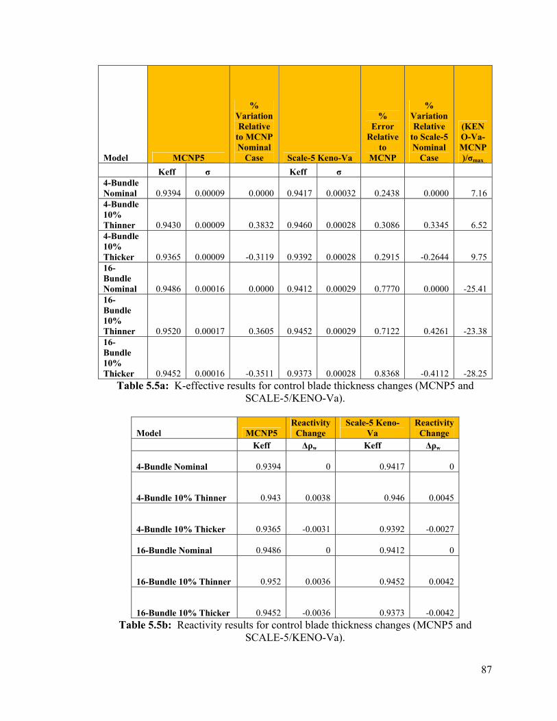
87
Model MCNP5
% Variation Relative
to MCNP Nominal
Case Scale-5 Keno-Va
% Error
Relative to
MCNP
% Variation Relative
to Scale-5 Nominal
Case
(KENO-Va-MCNP)/σmax
Keff σ Keff σ 4-Bundle Nominal 0.9394 0.00009 0.0000 0.9417 0.00032 0.2438 0.0000 7.16 4-Bundle 10% Thinner 0.9430 0.00009 0.3832 0.9460 0.00028 0.3086 0.3345 6.52 4-Bundle 10% Thicker 0.9365 0.00009 -0.3119 0.9392 0.00028 0.2915 -0.2644 9.75 16-Bundle Nominal 0.9486 0.00016 0.0000 0.9412 0.00029 0.7770 0.0000 -25.41 16-Bundle 10% Thinner 0.9520 0.00017 0.3605 0.9452 0.00029 0.7122 0.4261 -23.38 16-Bundle 10% Thicker 0.9452 0.00016 -0.3511 0.9373 0.00028 0.8368 -0.4112 -28.25
Table 5.5a: K-effective results for control blade thickness changes (MCNP5 and SCALE-5/KENO-Va).
Model MCNP5 Reactivity
Change Scale-5 Keno-
Va Reactivity
Change Keff Δρw Keff Δρw
4-Bundle Nominal 0.9394 0 0.9417 0
4-Bundle 10% Thinner 0.943 0.0038 0.946 0.0045
4-Bundle 10% Thicker 0.9365 -0.0031 0.9392 -0.0027
16-Bundle Nominal 0.9486 0 0.9412 0
16-Bundle 10% Thinner 0.952 0.0036 0.9452 0.0042
16-Bundle 10% Thicker 0.9452 -0.0036 0.9373 -0.0042 Table 5.5b: Reactivity results for control blade thickness changes (MCNP5 and
SCALE-5/KENO-Va).
88
The 10% thinner cases lead to an increase in the effective multiplication factor
between 0.33% - 0.43% from nominal. The 10% thicker cases all produced a decrease on
a similar scale, 0.26% - 0.41%. The (+/-) 10% thickness changes lead to overall
reactivity changes of about (+/-) 0.004 (Table 5.5b). Relative error for KENO-Va
compared to MCNP5 remained below one percent for this variation; however, a
maximum relative error of 0.84% occurred in the 16-bundle 10% thicker case. Very little
change in reactivity occurred because only control material volume, and not surface area,
was altered.
A 3 cm mesh was imposed for flux distributions, for all three blade thickness
cases, using MCNP5 and SCALE-5/KENO-Va. A cuboid-defined Global Unit was used
in the KENO-Va cases and all calculations were performed for the 4-bundle case.
Results are shown in Table 5.6 and Table 5.7 for the 10% thinner blade and 10% thicker
blade cases, respectively.
These tests provide the final validation for the flux calculation abilities of
SCALE-5/KENO-Va. The average flux percent error for KENO-Va, compared to
MCNP5, remained around 3 percent, 3.08% for the 10% thinner case and 3.21% for the
10% thicker case, where the nominal case had 3.23% error (Table 4.5). The volume
averaging error is present again but the overall results provide acceptable agreement
between the two code packages.
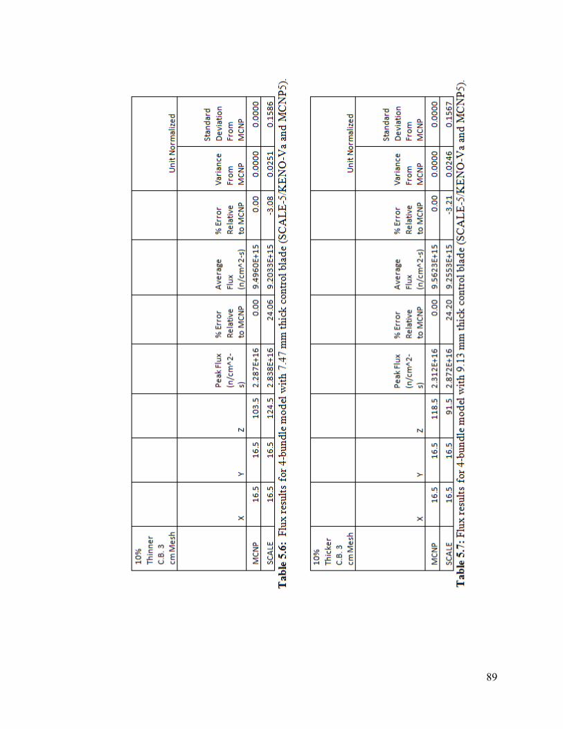
89
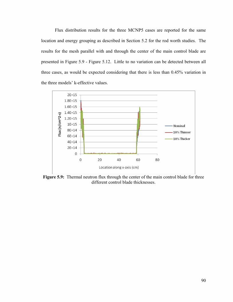
90
Flux distribution results for the three MCNP5 cases are reported for the same
location and energy grouping as described in Section 5.2 for the rod worth studies. The
results for the mesh parallel with and through the center of the main control blade are
presented in Figure 5.9 - Figure 5.12. Little to no variation can be detected between all
three cases, as would be expected considering that there is less than 0.45% variation in
the three models’ k-effective values.
Figure 5.9: Thermal neutron flux through the center of the main control blade for three
different control blade thicknesses.
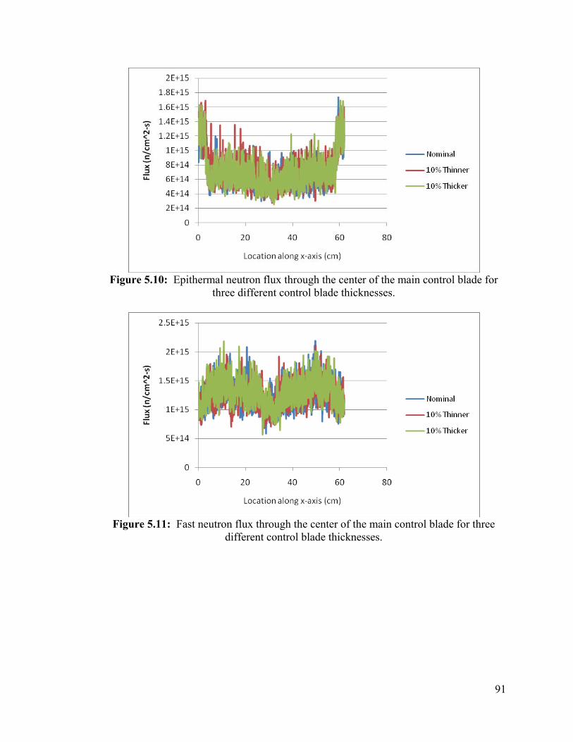
91
Figure 5.10: Epithermal neutron flux through the center of the main control blade for
three different control blade thicknesses.
Figure 5.11: Fast neutron flux through the center of the main control blade for three
different control blade thicknesses.
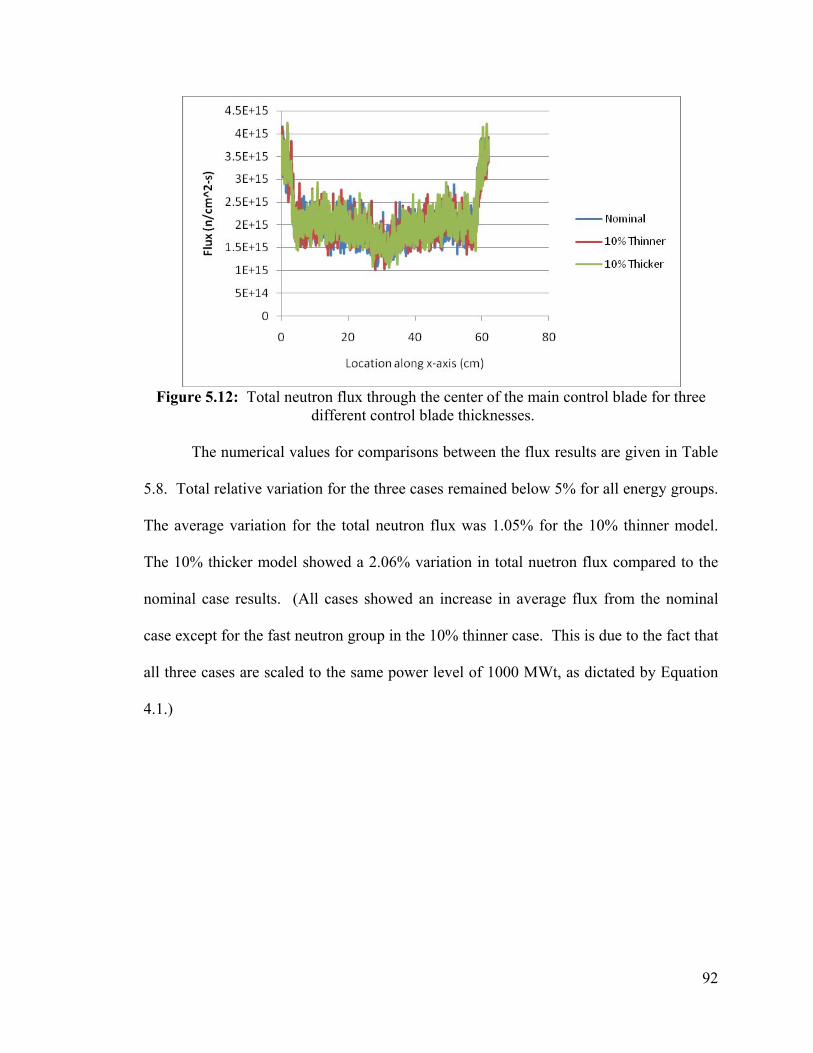
92
Figure 5.12: Total neutron flux through the center of the main control blade for three
different control blade thicknesses.
The numerical values for comparisons between the flux results are given in Table
5.8. Total relative variation for the three cases remained below 5% for all energy groups.
The average variation for the total neutron flux was 1.05% for the 10% thinner model.
The 10% thicker model showed a 2.06% variation in total nuetron flux compared to the
nominal case results. (All cases showed an increase in average flux from the nominal
case except for the fast neutron group in the 10% thinner case. This is due to the fact that
all three cases are scaled to the same power level of 1000 MWt, as dictated by Equation
4.1.)
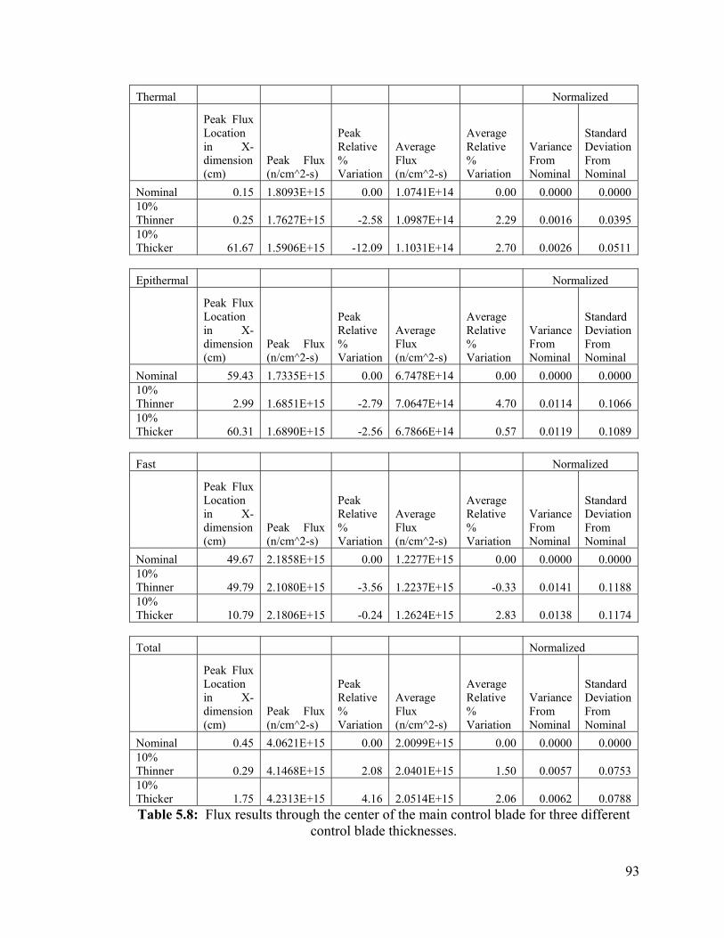
93
Thermal Normalized
Peak Flux Location in X-dimension (cm)
Peak Flux (n/cm^2-s)
Peak Relative % Variation
Average Flux (n/cm^2-s)
Average Relative % Variation
Variance From Nominal
Standard Deviation From Nominal
Nominal 0.15 1.8093E+15 0.00 1.0741E+14 0.00 0.0000 0.0000 10% Thinner 0.25 1.7627E+15 -2.58 1.0987E+14 2.29 0.0016 0.0395 10% Thicker 61.67 1.5906E+15 -12.09 1.1031E+14 2.70 0.0026 0.0511 Epithermal Normalized
Peak Flux Location in X-dimension (cm)
Peak Flux (n/cm^2-s)
Peak Relative % Variation
Average Flux (n/cm^2-s)
Average Relative % Variation
Variance From Nominal
Standard Deviation From Nominal
Nominal 59.43 1.7335E+15 0.00 6.7478E+14 0.00 0.0000 0.0000 10% Thinner 2.99 1.6851E+15 -2.79 7.0647E+14 4.70 0.0114 0.1066 10% Thicker 60.31 1.6890E+15 -2.56 6.7866E+14 0.57 0.0119 0.1089 Fast Normalized
Peak Flux Location in X-dimension (cm)
Peak Flux (n/cm^2-s)
Peak Relative % Variation
Average Flux (n/cm^2-s)
Average Relative % Variation
Variance From Nominal
Standard Deviation From Nominal
Nominal 49.67 2.1858E+15 0.00 1.2277E+15 0.00 0.0000 0.0000 10% Thinner 49.79 2.1080E+15 -3.56 1.2237E+15 -0.33 0.0141 0.1188 10% Thicker 10.79 2.1806E+15 -0.24 1.2624E+15 2.83 0.0138 0.1174 Total Normalized
Peak Flux Location in X-dimension (cm)
Peak Flux (n/cm^2-s)
Peak Relative % Variation
Average Flux (n/cm^2-s)
Average Relative % Variation
Variance From Nominal
Standard Deviation From Nominal
Nominal 0.45 4.0621E+15 0.00 2.0099E+15 0.00 0.0000 0.0000 10% Thinner 0.29 4.1468E+15 2.08 2.0401E+15 1.50 0.0057 0.0753 10% Thicker 1.75 4.2313E+15 4.16 2.0514E+15 2.06 0.0062 0.0788 Table 5.8: Flux results through the center of the main control blade for three different
control blade thicknesses.
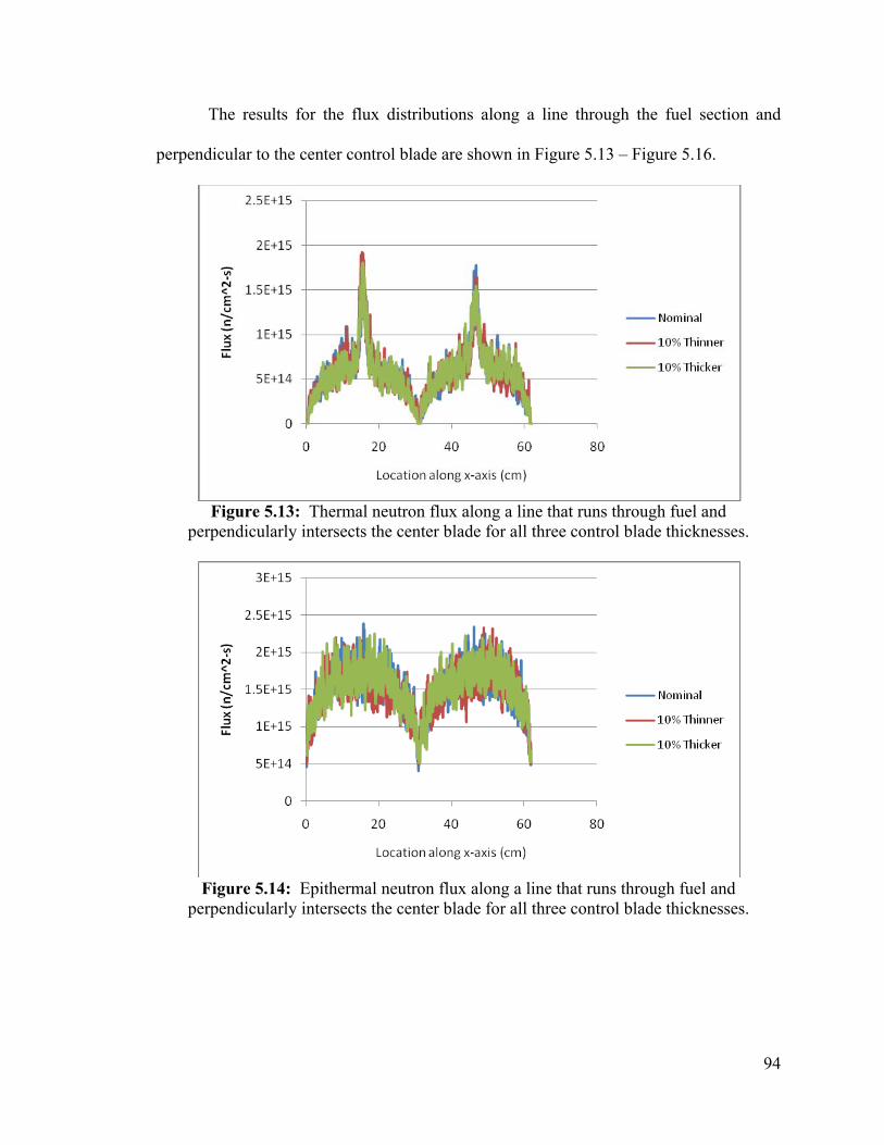
94
The results for the flux distributions along a line through the fuel section and
perpendicular to the center control blade are shown in Figure 5.13 – Figure 5.16.
Figure 5.13: Thermal neutron flux along a line that runs through fuel and
perpendicularly intersects the center blade for all three control blade thicknesses.
Figure 5.14: Epithermal neutron flux along a line that runs through fuel and
perpendicularly intersects the center blade for all three control blade thicknesses.
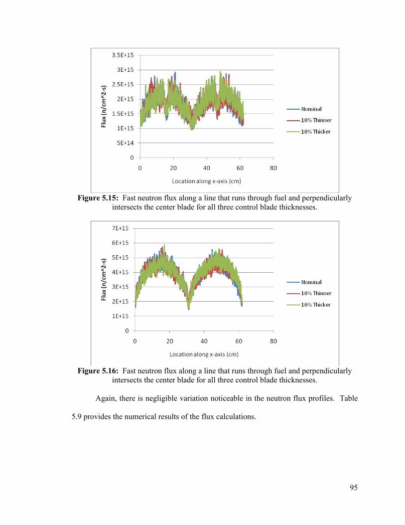
95
Figure 5.15: Fast neutron flux along a line that runs through fuel and perpendicularly
intersects the center blade for all three control blade thicknesses.
Figure 5.16: Fast neutron flux along a line that runs through fuel and perpendicularly
intersects the center blade for all three control blade thicknesses. Again, there is negligible variation noticeable in the neutron flux profiles. Table
5.9 provides the numerical results of the flux calculations.
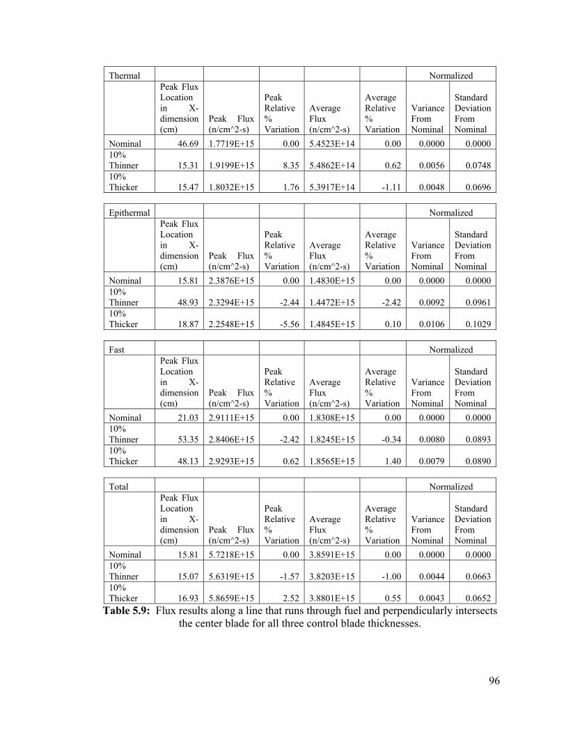
96
Thermal Normalized
Peak Flux Location in X-dimension (cm)
Peak Flux (n/cm^2-s)
Peak Relative % Variation
Average Flux (n/cm^2-s)
Average Relative % Variation
Variance From Nominal
Standard Deviation From Nominal
Nominal 46.69 1.7719E+15 0.00 5.4523E+14 0.00 0.0000 0.0000 10% Thinner 15.31 1.9199E+15 8.35 5.4862E+14 0.62 0.0056 0.0748 10% Thicker 15.47 1.8032E+15 1.76 5.3917E+14 -1.11 0.0048 0.0696 Epithermal Normalized
Peak Flux Location in X-dimension (cm)
Peak Flux (n/cm^2-s)
Peak Relative % Variation
Average Flux (n/cm^2-s)
Average Relative % Variation
Variance From Nominal
Standard Deviation From Nominal
Nominal 15.81 2.3876E+15 0.00 1.4830E+15 0.00 0.0000 0.0000 10% Thinner 48.93 2.3294E+15 -2.44 1.4472E+15 -2.42 0.0092 0.0961 10% Thicker 18.87 2.2548E+15 -5.56 1.4845E+15 0.10 0.0106 0.1029 Fast Normalized
Peak Flux Location in X-dimension (cm)
Peak Flux (n/cm^2-s)
Peak Relative % Variation
Average Flux (n/cm^2-s)
Average Relative % Variation
Variance From Nominal
Standard Deviation From Nominal
Nominal 21.03 2.9111E+15 0.00 1.8308E+15 0.00 0.0000 0.0000 10% Thinner 53.35 2.8406E+15 -2.42 1.8245E+15 -0.34 0.0080 0.0893 10% Thicker 48.13 2.9293E+15 0.62 1.8565E+15 1.40 0.0079 0.0890 Total Normalized
Peak Flux Location in X-dimension (cm)
Peak Flux (n/cm^2-s)
Peak Relative % Variation
Average Flux (n/cm^2-s)
Average Relative % Variation
Variance From Nominal
Standard Deviation From Nominal
Nominal 15.81 5.7218E+15 0.00 3.8591E+15 0.00 0.0000 0.0000 10% Thinner 15.07 5.6319E+15 -1.57 3.8203E+15 -1.00 0.0044 0.0663 10% Thicker 16.93 5.8659E+15 2.52 3.8801E+15 0.55 0.0043 0.0652
Table 5.9: Flux results along a line that runs through fuel and perpendicularly intersects the center blade for all three control blade thicknesses.
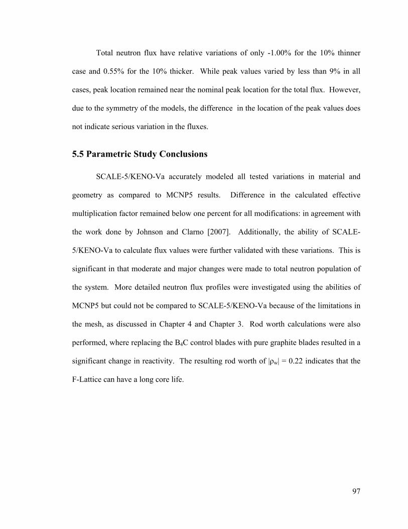
97
Total neutron flux have relative variations of only -1.00% for the 10% thinner
case and 0.55% for the 10% thicker. While peak values varied by less than 9% in all
cases, peak location remained near the nominal peak location for the total flux. However,
due to the symmetry of the models, the difference in the location of the peak values does
not indicate serious variation in the fluxes.
5.5 Parametric Study Conclusions
SCALE-5/KENO-Va accurately modeled all tested variations in material and
geometry as compared to MCNP5 results. Difference in the calculated effective
multiplication factor remained below one percent for all modifications: in agreement with
the work done by Johnson and Clarno [2007]. Additionally, the ability of SCALE-
5/KENO-Va to calculate flux values were further validated with these variations. This is
significant in that moderate and major changes were made to total neutron population of
the system. More detailed neutron flux profiles were investigated using the abilities of
MCNP5 but could not be compared to SCALE-5/KENO-Va because of the limitations in
the mesh, as discussed in Chapter 4 and Chapter 3. Rod worth calculations were also
performed, where replacing the B4C control blades with pure graphite blades resulted in a
significant change in reactivity. The resulting rod worth of |ρw| = 0.22 indicates that the
F-Lattice can have a long core life.
98
Chapter 6: Conclusions
6.1 Summary and Conclusion
The current resurgence of interest in the nuclear power industry has led to
renewed interest in new reactor designs. The GE Compact Modular Boiling Water
Reactor (CM-BWR) is one such reactor. The 350 MWe CM-BWR is designed for small
incremental additions to the power grid. A key feature of the CM-BWR is the use of the
unique F-Lattice. The F-Lattice employs a staggered row configuration for the control
blades. Additionally, the control blades are more than double the width of control blades
found in most commercial boiling water reactors today. Increase in blade width and pitch
allows for approximately a one-half factor decrease in the number of control blades.
Reduction in control blades results in a large reduction in control rod related components.
This reduces construction and maintenance costs, as well as reducing the risk of failures
within the core. However, before design certification can be completed for the CM-
BWR, first the tools needed to study and monitor reactor core performance must be
validated.
The purpose of this thesis was to validate the SCALE packages for the F-Lattice
design used in the CM-BWR core. This has been at least partially achieved in several
steps. The computational cost associated with SCALE-5.1/KENO-VI, SCALE-5/KENO-
VA and MCNP5 was determined. The limitations and advantages of each code were
discussed. It was found that SCALE-5.1/KENO-VI is very computationally intensive for
detailed analysis. Use of SCALE-5/KENO-VI, over MCNP5, for complex problems
99
requiring spatially detailed results is not recommended. Analysis of the F-Lattice with
SCALE-5/KENO-Va and SCALE-5.1/KENO-VI showed little difference in accuracy
compared to MCNP5. Therefore it was determined that SCALE-5/KENO-Va is not only
able to produce accurate results (k-effective and flux distributions) for the F-Lattice, but
it can do so much more efficiently than either SCALE-5.1/KENO-VI or MCNP5.
New techniques were developed to appropriately compare and validate the
SCALE-5/KENO-Va flux results. Average flux values were found to be accurate
(compared to MCNP5). However, only qualitative agreement was found for flux
distribution between the SCALE-5/KENO-Va and MCNP5 results. Cell specific flux
values may have significant error due to a “volume averaging” technique used in
normalizing the SCALE-5/KENO-Va flux results to the proper units. The “volume
“averaging” error was quantified by hand-calculations that produced SCALE-5 flux
results with less than one percent error compared to MCNP5 results. More accurate flux
results could not be achieved through mesh refinement due to memory and hard drive
limitations associated with SCALE-5/KENO-Va.
Parametric design studies, on material properties and geometry, were also
validated for SCALE-5/KENO-Va against MCNP5 benchmark results. The SCALE-
5/KENO-Va calculated k-effective values remained within one percent of MCNP5
benchmark results, and average flux calculations also remained within an acceptable
agreement of about 3%. Rod worth calculations led to a significant change in reactivity
resulting from the instantaneous removal of the B4C control blades. Therefore, gradual
removal of control blades is expected to produce a relatively long fuel lifetime. Fuel
100
burn-up calculations are still necessary to determine the core life (preliminary burn-up
results are provided in Appendix D).
In conclusion, SCALE-5/KENO-Va is found to be capable of efficient and
accurate results for the F-Lattice k-effective calculations. This is important because
minor variations in core configuration, such as testing different fuel compositions, can
now be trusted to be accurately modeled in SCALE-5. Additionally, the first steps to
validate neutron flux distributions calculated by SCALE-5 are developed in this thesis.
This will allow design engineers to test many different types of modifications to the F-
Lattice in a timely and efficient manner before using a more powerful and
computationally costly code, such as MCNP5, for the finer details of the system.
6.2 Future Work
There are many areas relating to the F-Lattice and to code validation for the
analysis of the F-Lattice that require further study. The primary suggestion for future
work would be testing the flux calculations of SCALE-5/KENO-Va with an even higher
level of mesh refinement. This could be done in two ways. The first would be to make
an adjustment to the SCALE-5 package source code. Suggested features to enhance
would be the ability to locally define the mesh size in each dimension. A restructuring of
the output file format should also be examined. A second alternative for testing the
accuracy of the flux calculations would be to use a supercomputer with a very large
memory and hard drive space. It is believed that it is a simple hardware limitation that is
preventing a more refined mesh to be analyzed with SCALE-5. Access to more powerful
computers could prove both the validity of that claim, as well as allow a more meaningful
comparison to the MCNP5 results. Work to eliminate the volume averaging error
101
discussed in this thesis should also be explored. This would require developing the tools
to read the SCALE-5/KENO-Va geometry and mesh size and carry out individual volume
calculations on a cell by cell basis. It is important to develop an automated tool to
perform these calculations because geometry and mesh size can vary dramatically
depending on the model being studied.
Additional relevant work is to explore deterministic codes for k-effective and
power distribution calculations. Most likely this would start with the 4-bundle case, as it
is the simplest representation of the F-Lattice. A deterministic approach may suggest an
even more efficient means of parametric design studies. There are additional design
parameters that need to be explored in greater detail. Significantly increased moderator
pitch will affect the system thermo-hydraulics and should also be investigated more
thoroughly. Finally, an investigation into isotopic burn-up and core life would provide
crucial insight on the viability of the F-Lattice. A preliminary burn-up analysis of the 4-
bundle case is given in Appendix D. (An “average” reactor assembly is burned for 1
month, in 1 day increments, and for 20 months, in 2 week increments. The control blades
remain fully inserted for the entire duration of fuel burn.)
This thesis has provided the initial steps in validating the SCALE-5 package to
analyze the F-Lattice design. K-effective and average flux values evaluated by SCALE-5
have been shown to be accurate. The package also evaluates accurate flux (power)
distributions, though accurately extracting that information for comparison with MCNP5
results is not straight forward. Further validation for additional parametric studies and
burn-up calculations are likely to “validate” the code for the F-Lattice design analysis.
102
References
Busch, R.D. and Bowman, S.M.. KENO V.a Primer: A Primer for Criticality iiiiiiiiiiCalculations with SCALE/KENO V.a Using GeeWiz. Report ORNL/TM-iiiiiiiiii2005/135, Oak Ridge National Laboratory, 2005. Challberg, R.C., “Simplified Core and Internals Design for the ESBWR,” Proceedings 6th iiiiiiiiiInternational Conference on Nuclear Engineering, (1998), ICONE-6066. Clarno, K. et al., “Code-to-Code Benchmark of Coolant Void Reactivity (CVR) in the iiiiiiiiiACR-700 Reactor,” ANS Transactions 93 (2005): 372-375. Duderstadt, James J. and Hamilton, Louis J., Nuclear Reactor Analysis. New York: John iiiiiiiiiWiley and Sons, 1976. Dupree, Stephen A. and Fraley, Stanley K, A Monte Carlo Primer: A Practical Approach iiiiiiiiiito Radiation Transport. New York: Kluwer Academic/Plenum Publishers, 2003. Fennern, L. et al., “Compact Modular BWR (CM-BWR).” International Conference on iiiiiiiiiiGlobal Environment and Advanced Nuclear Power Plants 1012: (2003). Johnson, S. and Clarno, K. “Comparison of SCALE and MCNP Results for iiiiiiiiiiComputational Pebble Bed Benchmarks,” ANS Transactions (2007). Lamarsh, John R., Introduction to Nuclear Reactor Theory. Reading, Mass.: Addison - Wesley Pub. Co, 1966. Landau, Rubin H., Páez, Manuel José and Bordeianu, Cristian C., Computational iiiiiiiiiiiPhysics, Problem Solving with Computers, 2nd ed. WILEY-VCH Verlag GMbH iiiiiiiiiii& Co. KGaA, Weinheim, 2007. Lemey, L. and Colburn, R., Sams Teach Yourself Perl in 21 Days, 2nd ed. Sams ……..Publishing, 2007. Ragheb, M, “NPRE498 Monte Carlo Method Chapter 1,” 2007, <https://netfiles.uiuc.edu/ Mmm mragheb/www/> (2 September 2007). Reis, V. et al., “Nuclear Fuel Leasing, Recycling, and Proliferation: Modeling A Global ,,,,,,,,,,,View,” Nuclear Technology 150 (2005): 121-131. SCALE: A Modular Code System for Performing Standardized Computer Analysis for ,,,,,,,,,,,Licensing Evaluations. Report ORNL/TM-2005/39, Version 5, Vols I-III, Oak mmm Ridge National Laboratory, 2005.
103
SwiftGear. Large Text File Viewer 4u. 24 October 2005. <http://www.swiftgear.com> (3 April 2008) Tari, Ilker. Homogenized Cross Section Determination using Monte Carlo Simulation.
MS Thesis: Massachusetts Institute of Technology, 1994. U.S. Department of Energy. Office of Nuclear Energy. Office of Fuel Cycle iiiiiiiiiiManagement. Global Nuclear Energy Partnership Strategic Plan, 2007. GNEP-iiiiiiiiii167312, Rev. 0. X-5 Monte Carlo Team. MCNP - General Monte Carlo N-paricle Transport Code, iiiiiiiiiiVersion 5. Los Alamos National Laboratory, 2003.
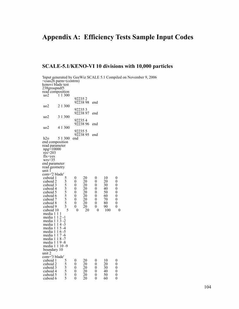
104
Appendix A: Efficiency Tests Sample Input Codes
SCALE-5.1/KENO-VI 10 divisions with 10,000 particles 'Input generated by GeeWiz SCALE 5.1 Compiled on November 9, 2006 =csas26 parm=(centrm) kenovi blade test 238groupndf5 read composition uo2 1 1 300 92235 2 92238 98 end uo2 2 1 300 92235 3 92238 97 end uo2 3 1 300 92235 4 92238 96 end uo2 4 1 300 92235 5 92238 95 end h2o 5 1 300 end end composition read parameter npg=10000 res=203 flx=yes wrs=35 end parameter read geometry unit 1 com='2 blade' cuboid 1 5 0 20 0 10 0 cuboid 2 5 0 20 0 20 0 cuboid 3 5 0 20 0 30 0 cuboid 4 5 0 20 0 40 0 cuboid 5 5 0 20 0 50 0 cuboid 6 5 0 20 0 60 0 cuboid 7 5 0 20 0 70 0 cuboid 8 5 0 20 0 80 0 cuboid 9 5 0 20 0 90 0 cuboid 10 5 0 20 0 100 0 media 1 1 1 media 1 1 2 -1 media 1 1 3 -2 media 1 1 4 -3 media 1 1 5 -4 media 1 1 6 -5 media 1 1 7 -6 media 1 1 8 -7 media 1 1 9 -8 media 1 1 10 -9 boundary 10 unit 2 com='3 blade' cuboid 1 5 0 20 0 10 0 cuboid 2 5 0 20 0 20 0 cuboid 3 5 0 20 0 30 0 cuboid 4 5 0 20 0 40 0 cuboid 5 5 0 20 0 50 0 cuboid 6 5 0 20 0 60 0
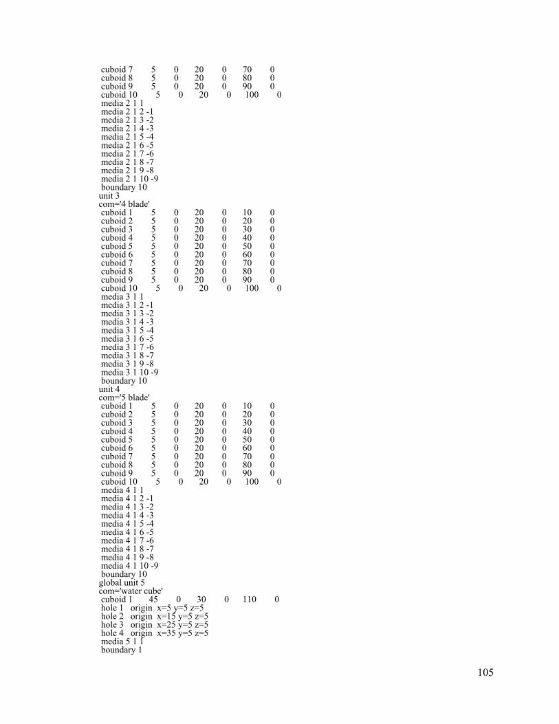
105
cuboid 7 5 0 20 0 70 0 cuboid 8 5 0 20 0 80 0 cuboid 9 5 0 20 0 90 0 cuboid 10 5 0 20 0 100 0 media 2 1 1 media 2 1 2 -1 media 2 1 3 -2 media 2 1 4 -3 media 2 1 5 -4 media 2 1 6 -5 media 2 1 7 -6 media 2 1 8 -7 media 2 1 9 -8 media 2 1 10 -9 boundary 10 unit 3 com='4 blade' cuboid 1 5 0 20 0 10 0 cuboid 2 5 0 20 0 20 0 cuboid 3 5 0 20 0 30 0 cuboid 4 5 0 20 0 40 0 cuboid 5 5 0 20 0 50 0 cuboid 6 5 0 20 0 60 0 cuboid 7 5 0 20 0 70 0 cuboid 8 5 0 20 0 80 0 cuboid 9 5 0 20 0 90 0 cuboid 10 5 0 20 0 100 0 media 3 1 1 media 3 1 2 -1 media 3 1 3 -2 media 3 1 4 -3 media 3 1 5 -4 media 3 1 6 -5 media 3 1 7 -6 media 3 1 8 -7 media 3 1 9 -8 media 3 1 10 -9 boundary 10 unit 4 com='5 blade' cuboid 1 5 0 20 0 10 0 cuboid 2 5 0 20 0 20 0 cuboid 3 5 0 20 0 30 0 cuboid 4 5 0 20 0 40 0 cuboid 5 5 0 20 0 50 0 cuboid 6 5 0 20 0 60 0 cuboid 7 5 0 20 0 70 0 cuboid 8 5 0 20 0 80 0 cuboid 9 5 0 20 0 90 0 cuboid 10 5 0 20 0 100 0 media 4 1 1 media 4 1 2 -1 media 4 1 3 -2 media 4 1 4 -3 media 4 1 5 -4 media 4 1 6 -5 media 4 1 7 -6 media 4 1 8 -7 media 4 1 9 -8 media 4 1 10 -9 boundary 10 global unit 5 com='water cube' cuboid 1 45 0 30 0 110 0 hole 1 origin x=5 y=5 z=5 hole 2 origin x=15 y=5 z=5 hole 3 origin x=25 y=5 z=5 hole 4 origin x=35 y=5 z=5 media 5 1 1 boundary 1
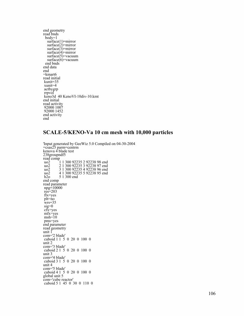
106
end geometry read bnds body=1 surface(1)=mirror surface(2)=mirror surface(3)=mirror surface(4)=mirror surface(5)=vacuum surface(6)=vacuum end bnds end data end =kmart6 read initial kunit=35 xunit=4 actbygrp rrpvol keno3d 40 KenoVI-10div-10.kmt end initial read activity 92000 1007 92000 1452 end activity end
SCALE-5/KENO-Va 10 cm mesh with 10,000 particles 'Input generated by GeeWiz 5.0 Compiled on 04-30-2004 =csas25 parm=centrm kenova 4 blade test 238groupndf5 read comp uo2 1 1 300 92235 2 92238 98 end uo2 2 1 300 92235 3 92238 97 end uo2 3 1 300 92235 4 92238 96 end uo2 4 1 300 92235 5 92238 95 end h2o 5 1 300 end end comp read parameter npg=10000 res=203 flx=yes plt=no wrs=35 sig=0 cfx=yes mfx=yes msh=10 pms=yes end parameter read geometry unit 1 com='2 blade' cuboid 1 1 5 0 20 0 100 0 unit 2 com='3 blade' cuboid 2 1 5 0 20 0 100 0 unit 3 com='4 blade' cuboid 3 1 5 0 20 0 100 0 unit 4 com='5 blade' cuboid 4 1 5 0 20 0 100 0 global unit 5 com='cube reactor' cuboid 5 1 45 0 30 0 110 0
107
hole 4 35 5 5 hole 3 25 5 5 hole 2 15 5 5 hole 1 5 5 5 end geometry read bnds +xb=mirror -xb=mirror +yb=mirror -yb=mirror +zb=vacuum -zb=vacuum end bnds end data end =kmart read initial kunit=35 xunit=4 actbygrp rrpvol keno3d 40 KenoVa-10cm10.kmt end initial read activity 92000 1007 92000 1452 end activity end
MCNP5 10 cm mesh with 10,000 particles 4 Blade Test vs. SCALE5 C Cell Cards 1 1 -10.96 1 -2 3 -4 5 -6 imp:n=1 $ block 1 2 like 1 but mat=2 rho=-10.96 trcl=(10 0 0) 3 like 1 but mat=3 rho=-10.96 trcl=(20 0 0) 4 like 1 but mat=4 rho=-10.96 trcl=(30 0 0) 5 5 -0.9982 7 -8 9 -10 11 -12 #1 #2 #3 #4 imp:n=1 6 0 -7:8:-9:10:-11:12 imp:n=0 C Surface Cards 1 px 5.0 2 px 10.0 3 py 5.0 4 py 25.0 5 pz 5.0 6 pz 105.0 7 -7 px 0.0 8 -8 px 45.0 9 -9 py 0.0 10 -10 py 30.0 11 pz 0.0 12 pz 110.0 C Data Cards C Material Cards m1 92235.66c 5.1234e-5 92238.66c 0.002454 8016.66c 0.00506 m2 92235.66c 7.6851e-5 92238.66c 0.002479 8016.66c 0.005061 m3 92235.66c 1.02468e-4 92238.66c 0.002428 8016.66c 0.005061 m4 92235.66c 1.28085e-4 92238.66c 0.002403 8016.66c 0.005062 m5 1001.62c 2 8016.62c 1 mt5 lwtr.60t C Control Cards

108
kcode 10000 1.0 50 203 ksrc 7.5 15 36.6 7.5 15 73.3 17.5 15 36.6 17.5 15 73.3 27.5 15 36.6 27.5 15 73.3 37.5 15 36.6 37.5 15 73.3 FMESH4:n GEOM=xyz ORIGIN=0 0 0 IMESH=50 IINTS=5 JMESH=30 JINTS=3 KMESH=110 KINTS=11
109
Appendix B: 4-bundle and 16-bundle Sample Input Files SCALE-5/KENO-Va 4-bundle cell input file using a cuboid-defined global array and 3 cm mesh 'Input generated by GeeWiz 5.0 Compiled on 04-30-2004 =csas25 parm=centrm 4x4 kenova assembly 238groupndf5 read comp uo2 1 1 300 92235 2.5 92238 97.5 end zirc4 2 den=6.489 1 300 end ss304s 3 den=8 1 300 end h2o 4 den=1 1 300 end b4c 5 1 300 end end comp read celldata latticecell squarepitch fuelr=0.5544 1 gapr=0.5628 0 cladr=0.65352 2 hpitch=0.8505 4 end more data szf=0.1 end more end celldata read parameter gen=800 npg=10000 nsk=250 res=250 flx=yes fdn=yes plt=no wrs=35 sig=0 cfx=yes pnm=0 pmf=yes mfx=yes msh=3 pms=yes end parameter read geometry unit 1 com='fuel cell unit' zcylinder 1 1 0.5544 274.3 0 zcylinder 0 1 0.5628 274.3 0 zcylinder 2 1 0.65352 274.3 0 cuboid 4 1 0.8505 -0.8505 0.8505 -0.8505 274.3 0 unit 2 com='bundle and canister (2,2), (2,4), (4,2) and (4,4)' array 1 0.1535 0.1535 0 cuboid 4 1 13.7615 0.1535 13.7615 0.1535 274.3 0 cuboid 3 1 13.915 0 13.915 0 274.3 0 unit 3 com='water in x (3,2) and (3,4)' cuboid 4 1 13.915 0 1.575 0 274.3 0 unit 4 com='water in y (2,3) and (4,3)' cuboid 4 1 1.575 0 13.915 0 274.3 0 unit 5 com='water in center (3,3)' cuboid 4 1 1.575 0 1.575 0 274.3 0 unit 6 com='left longest y cb (4,1)'
110
cuboid 5 1 0.415 0 13.915 0 274.3 15.2 cuboid 4 1 0.79 0 13.915 0 274.3 0 unit 7 com='left short y cb (3,1)' cuboid 5 1 0.415 0 1.575 0 274.3 15.2 cuboid 4 1 0.79 0 1.575 0 274.3 0 unit 8 com='left medium y cb (2,1)' cuboid 5 1 0.415 0 11.12 0 274.3 15.2 cuboid 4 1 0.79 0 13.915 0 274.3 0 unit 9 com='bottom longest x cb (5,2)' cuboid 5 1 13.915 0 0.415 0 274.3 15.2 cuboid 4 1 13.915 0 0.79 0 274.3 0 unit 10 com='bottom short x cb (5,3)' cuboid 5 1 1.575 0 0.415 0 274.3 15.2 cuboid 4 1 1.575 0 0.79 0 274.3 0 unit 11 com='bottom medium x cb ((5,4)' cuboid 5 1 11.12 0 0.415 0 274.3 15.2 cuboid 4 1 13.915 0 0.79 0 274.3 0 unit 12 com='right longest y cb (2,5)' cuboid 5 1 0.79 0.375 13.915 0 274.3 15.2 cuboid 4 1 0.79 0 13.915 0 274.3 0 unit 13 com='right short y cb (3,5)' cuboid 5 1 0.79 0.375 1.575 0 274.3 15.2 cuboid 4 1 0.79 0 1.575 0 274.3 0 unit 14 com='right medium y cb (4,5)' cuboid 5 1 0.79 0.375 13.915 2.795 274.3 15.2 cuboid 4 1 0.79 0 13.915 0 274.3 0 unit 15 com='top longest x cb (1,4)' cuboid 5 1 13.915 0 0.79 0.375 274.3 15.2 cuboid 4 1 13.915 0 0.79 0 274.3 0 unit 16 com='top short x cb (1,3)' cuboid 5 1 1.575 0 0.79 0.375 274.3 15.2 cuboid 4 1 1.575 0 0.79 0 274.3 0 unit 17 com='top medium x cb (1,2)' cuboid 5 1 13.915 2.795 0.79 0.375 274.3 15.2 cuboid 4 1 13.915 0 0.79 0 274.3 0 unit 18 com='corner squares of water (1,1) and (5,5)' cuboid 4 1 0.79 0 0.79 0 274.3 0 unit 19 com='short x corner cb (lines up with 21)' cuboid 5 1 0.415 0 0.415 0 274.3 15.2 cuboid 4 1 0.415 0 0.415 0 274.3 0 unit 20 com='long x corner cb (lines up with 22)' cuboid 5 1 0.375 0 0.415 0 274.3 15.2 cuboid 4 1 0.375 0 0.415 0 274.3 0 unit 21 com='corner y cb (shorter than corner x) (with 19)' cuboid 5 1 0.415 0 0.375 0 274.3 15.2 cuboid 4 1 0.415 0 0.375 0 274.3 0 unit 22 com='corner water square (with 20)' cuboid 4 1 0.375 0 0.375 0 274.3 0 unit 23 com='bottom left corner cb (5,1)' array 2 0 0 0 unit 24 com='top right corner cb (1,5)' array 3 30.195 30.195 0
111
global unit 25 array 4 0 0 0 end geometry read array ara=1 nux=8 nuy=8 nuz=1 fill 64*1 end fill ara=2 nux=2 nuy=2 nuz=1 fill 19 20 21 22 end fill ara=3 nux=2 nuy=2 nuz=1 fill 22 21 20 19 end fill ara=4 nux=5 nuy=5 nuz=1 fill 23 9 10 11 18 6 2 4 2 14 7 3 5 3 13 8 2 4 2 12 18 17 16 15 24 end fill end array read plot scr=yes ttl='test plot ncr' pic=mixtures xul=0 yul=30.98 zul=137.15 xlr=30.98 ylr=0 zlr=137.15 nax=800 clr=1 255 0 0 2 0 0 205 3 0 229 238 4 0 238 0 5 205 205 0 end color uax=1 vdn=-1 end end plot read bnds +xb=mirror -xb=mirror +yb=mirror -yb=mirror +zb=vacuum -zb=vacuum end bnds end data end =kmart read initial kunit=35 xunit=4 actbygrp rrpvol keno3d 40 3cm_MeshUpdateInUnit.kmt end initial read activity 92000 1007 92000 1452 end activity end
SCALE-5/KENO-Va 16-bundle cell input file 'Input generated by GeeWiz 5.0 Compiled on 04-30-2004 =csas25 parm=centrm 16 bundle 238groupndf5 read comp
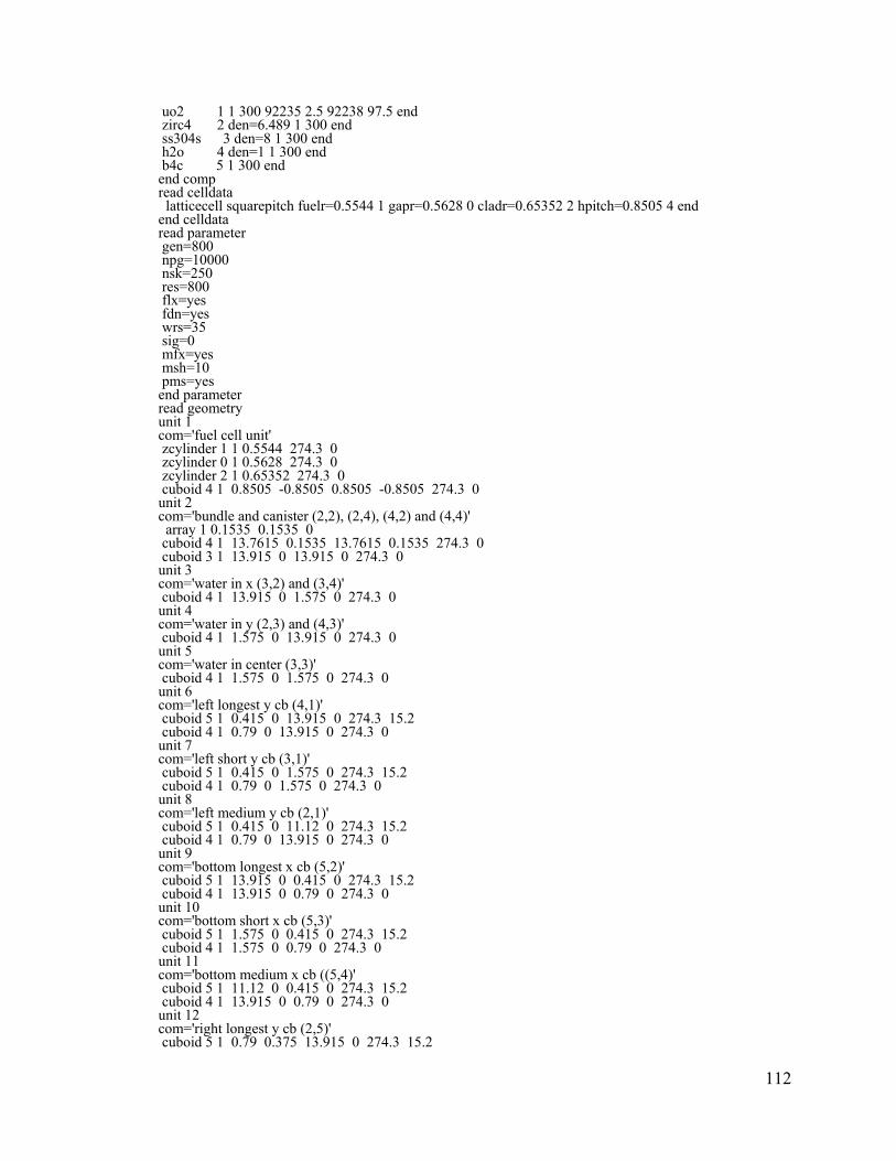
112
uo2 1 1 300 92235 2.5 92238 97.5 end zirc4 2 den=6.489 1 300 end ss304s 3 den=8 1 300 end h2o 4 den=1 1 300 end b4c 5 1 300 end end comp read celldata latticecell squarepitch fuelr=0.5544 1 gapr=0.5628 0 cladr=0.65352 2 hpitch=0.8505 4 end end celldata read parameter gen=800 npg=10000 nsk=250 res=800 flx=yes fdn=yes wrs=35 sig=0 mfx=yes msh=10 pms=yes end parameter read geometry unit 1 com='fuel cell unit' zcylinder 1 1 0.5544 274.3 0 zcylinder 0 1 0.5628 274.3 0 zcylinder 2 1 0.65352 274.3 0 cuboid 4 1 0.8505 -0.8505 0.8505 -0.8505 274.3 0 unit 2 com='bundle and canister (2,2), (2,4), (4,2) and (4,4)' array 1 0.1535 0.1535 0 cuboid 4 1 13.7615 0.1535 13.7615 0.1535 274.3 0 cuboid 3 1 13.915 0 13.915 0 274.3 0 unit 3 com='water in x (3,2) and (3,4)' cuboid 4 1 13.915 0 1.575 0 274.3 0 unit 4 com='water in y (2,3) and (4,3)' cuboid 4 1 1.575 0 13.915 0 274.3 0 unit 5 com='water in center (3,3)' cuboid 4 1 1.575 0 1.575 0 274.3 0 unit 6 com='left longest y cb (4,1)' cuboid 5 1 0.415 0 13.915 0 274.3 15.2 cuboid 4 1 0.79 0 13.915 0 274.3 0 unit 7 com='left short y cb (3,1)' cuboid 5 1 0.415 0 1.575 0 274.3 15.2 cuboid 4 1 0.79 0 1.575 0 274.3 0 unit 8 com='left medium y cb (2,1)' cuboid 5 1 0.415 0 11.12 0 274.3 15.2 cuboid 4 1 0.79 0 13.915 0 274.3 0 unit 9 com='bottom longest x cb (5,2)' cuboid 5 1 13.915 0 0.415 0 274.3 15.2 cuboid 4 1 13.915 0 0.79 0 274.3 0 unit 10 com='bottom short x cb (5,3)' cuboid 5 1 1.575 0 0.415 0 274.3 15.2 cuboid 4 1 1.575 0 0.79 0 274.3 0 unit 11 com='bottom medium x cb ((5,4)' cuboid 5 1 11.12 0 0.415 0 274.3 15.2 cuboid 4 1 13.915 0 0.79 0 274.3 0 unit 12 com='right longest y cb (2,5)' cuboid 5 1 0.79 0.375 13.915 0 274.3 15.2
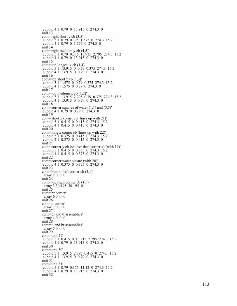
113
cuboid 4 1 0.79 0 13.915 0 274.3 0 unit 13 com='right short y cb (3,5)' cuboid 5 1 0.79 0.375 1.575 0 274.3 15.2 cuboid 4 1 0.79 0 1.575 0 274.3 0 unit 14 com='right medium y cb (4,5)' cuboid 5 1 0.79 0.375 13.915 2.795 274.3 15.2 cuboid 4 1 0.79 0 13.915 0 274.3 0 unit 15 com='top longest x cb (1,4)' cuboid 5 1 13.915 0 0.79 0.375 274.3 15.2 cuboid 4 1 13.915 0 0.79 0 274.3 0 unit 16 com='top short x cb (1,3)' cuboid 5 1 1.575 0 0.79 0.375 274.3 15.2 cuboid 4 1 1.575 0 0.79 0 274.3 0 unit 17 com='top medium x cb (1,2)' cuboid 5 1 13.915 2.795 0.79 0.375 274.3 15.2 cuboid 4 1 13.915 0 0.79 0 274.3 0 unit 18 com='corner squares of water (1,1) and (5,5)' cuboid 4 1 0.79 0 0.79 0 274.3 0 unit 19 com='short x corner cb (lines up with 21)' cuboid 5 1 0.415 0 0.415 0 274.3 15.2 cuboid 4 1 0.415 0 0.415 0 274.3 0 unit 20 com='long x corner cb (lines up with 22)' cuboid 5 1 0.375 0 0.415 0 274.3 15.2 cuboid 4 1 0.375 0 0.415 0 274.3 0 unit 21 com='corner y cb (shorter than corner x) (with 19)' cuboid 5 1 0.415 0 0.375 0 274.3 15.2 cuboid 4 1 0.415 0 0.375 0 274.3 0 unit 22 com='corner water square (with 20)' cuboid 4 1 0.375 0 0.375 0 274.3 0 unit 23 com='bottom left corner cb (5,1)' array 2 0 0 0 unit 24 com='top right corner cb (1,5)' array 3 30.195 30.195 0 unit 25 com='br corner' array 6 0 0 0 unit 26 com='tl corner' array 7 0 0 0 unit 27 com='br and tl assemblies' array 4 0 0 0 unit 28 com='tl and br assemblies' array 5 0 0 0 unit 29 com='unit 29' cuboid 5 1 0.415 0 13.915 2.795 274.3 15.2 cuboid 4 1 0.79 0 13.915 0 274.3 0 unit 30 com='unit 30' cuboid 5 1 13.915 2.795 0.415 0 274.3 15.2 cuboid 4 1 13.915 0 0.79 0 274.3 0 unit 31 com='unit 31' cuboid 5 1 0.79 0.375 11.12 0 274.3 15.2 cuboid 4 1 0.79 0 13.915 0 274.3 0 unit 32
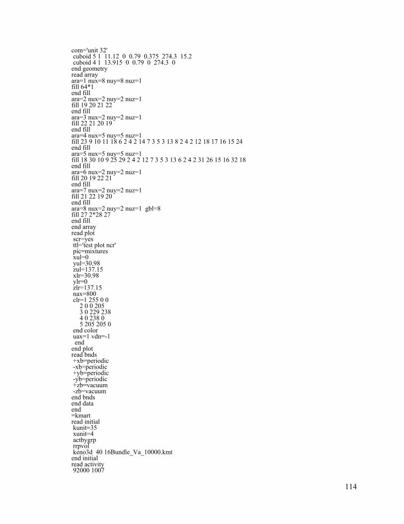
114
com='unit 32' cuboid 5 1 11.12 0 0.79 0.375 274.3 15.2 cuboid 4 1 13.915 0 0.79 0 274.3 0 end geometry read array ara=1 nux=8 nuy=8 nuz=1 fill 64*1 end fill ara=2 nux=2 nuy=2 nuz=1 fill 19 20 21 22 end fill ara=3 nux=2 nuy=2 nuz=1 fill 22 21 20 19 end fill ara=4 nux=5 nuy=5 nuz=1 fill 23 9 10 11 18 6 2 4 2 14 7 3 5 3 13 8 2 4 2 12 18 17 16 15 24 end fill ara=5 nux=5 nuy=5 nuz=1 fill 18 30 10 9 25 29 2 4 2 12 7 3 5 3 13 6 2 4 2 31 26 15 16 32 18 end fill ara=6 nux=2 nuy=2 nuz=1 fill 20 19 22 21 end fill ara=7 nux=2 nuy=2 nuz=1 fill 21 22 19 20 end fill ara=8 nux=2 nuy=2 nuz=1 gbl=8 fill 27 2*28 27 end fill end array read plot scr=yes ttl='test plot ncr' pic=mixtures xul=0 yul=30.98 zul=137.15 xlr=30.98 ylr=0 zlr=137.15 nax=800 clr=1 255 0 0 2 0 0 205 3 0 229 238 4 0 238 0 5 205 205 0 end color uax=1 vdn=-1 end end plot read bnds +xb=periodic -xb=periodic +yb=periodic -yb=periodic +zb=vacuum -zb=vacuum end bnds end data end =kmart read initial kunit=35 xunit=4 actbygrp rrpvol keno3d 40 16Bundle_Va_10000.kmt end initial read activity 92000 1007
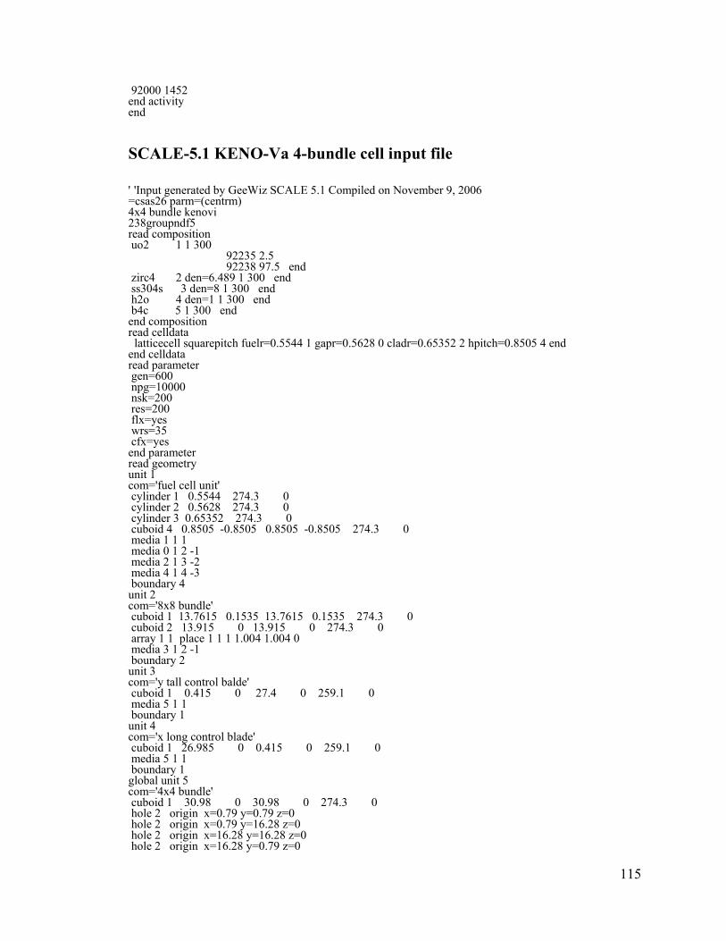
115
92000 1452 end activity end
SCALE-5.1 KENO-Va 4-bundle cell input file ' 'Input generated by GeeWiz SCALE 5.1 Compiled on November 9, 2006 =csas26 parm=(centrm) 4x4 bundle kenovi 238groupndf5 read composition uo2 1 1 300 92235 2.5 92238 97.5 end zirc4 2 den=6.489 1 300 end ss304s 3 den=8 1 300 end h2o 4 den=1 1 300 end b4c 5 1 300 end end composition read celldata latticecell squarepitch fuelr=0.5544 1 gapr=0.5628 0 cladr=0.65352 2 hpitch=0.8505 4 end end celldata read parameter gen=600 npg=10000 nsk=200 res=200 flx=yes wrs=35 cfx=yes end parameter read geometry unit 1 com='fuel cell unit' cylinder 1 0.5544 274.3 0 cylinder 2 0.5628 274.3 0 cylinder 3 0.65352 274.3 0 cuboid 4 0.8505 -0.8505 0.8505 -0.8505 274.3 0 media 1 1 1 media 0 1 2 -1 media 2 1 3 -2 media 4 1 4 -3 boundary 4 unit 2 com='8x8 bundle' cuboid 1 13.7615 0.1535 13.7615 0.1535 274.3 0 cuboid 2 13.915 0 13.915 0 274.3 0 array 1 1 place 1 1 1 1.004 1.004 0 media 3 1 2 -1 boundary 2 unit 3 com='y tall control balde' cuboid 1 0.415 0 27.4 0 259.1 0 media 5 1 1 boundary 1 unit 4 com='x long control blade' cuboid 1 26.985 0 0.415 0 259.1 0 media 5 1 1 boundary 1 global unit 5 com='4x4 bundle' cuboid 1 30.98 0 30.98 0 274.3 0 hole 2 origin x=0.79 y=0.79 z=0 hole 2 origin x=0.79 y=16.28 z=0 hole 2 origin x=16.28 y=16.28 z=0 hole 2 origin x=16.28 y=0.79 z=0
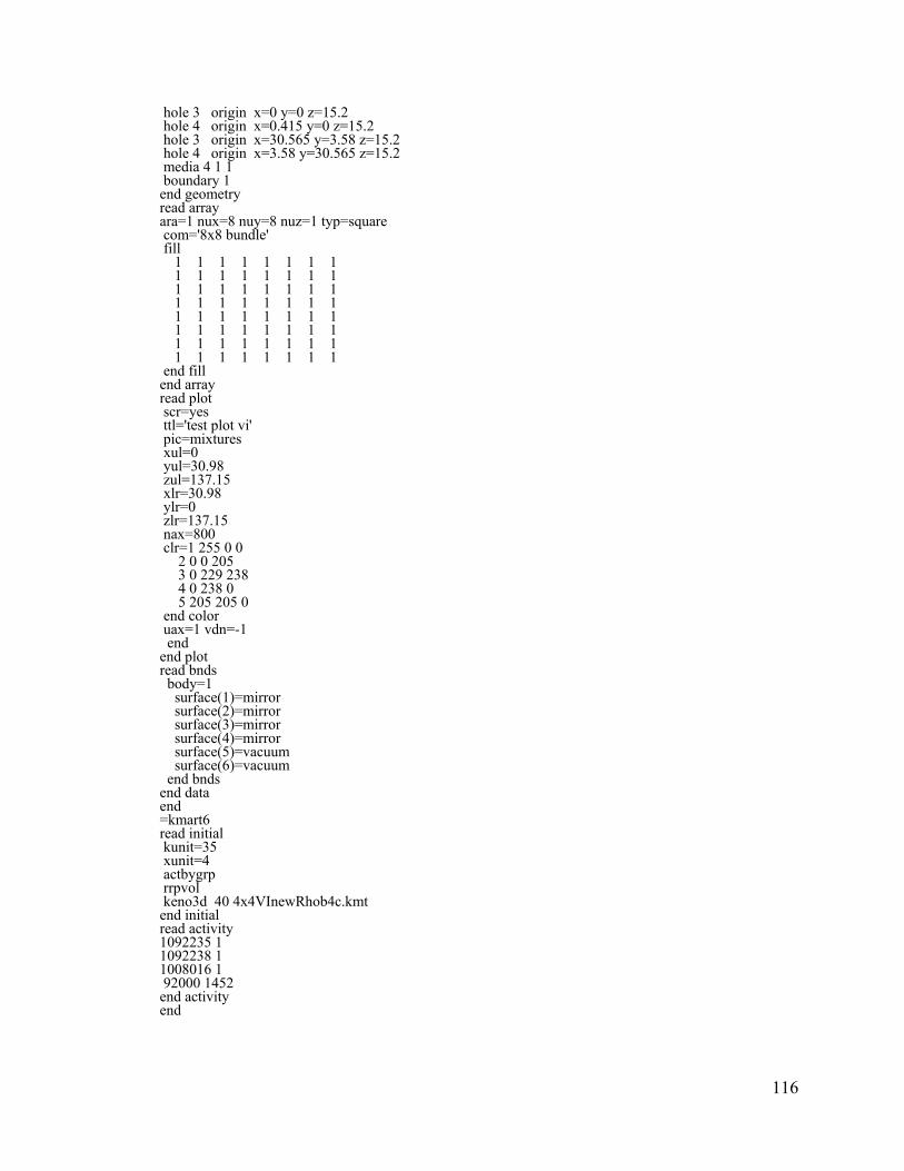
116
hole 3 origin x=0 y=0 z=15.2 hole 4 origin x=0.415 y=0 z=15.2 hole 3 origin x=30.565 y=3.58 z=15.2 hole 4 origin x=3.58 y=30.565 z=15.2 media 4 1 1 boundary 1 end geometry read array ara=1 nux=8 nuy=8 nuz=1 typ=square com='8x8 bundle' fill 1 1 1 1 1 1 1 1 1 1 1 1 1 1 1 1 1 1 1 1 1 1 1 1 1 1 1 1 1 1 1 1 1 1 1 1 1 1 1 1 1 1 1 1 1 1 1 1 1 1 1 1 1 1 1 1 1 1 1 1 1 1 1 1 end fill end array read plot scr=yes ttl='test plot vi' pic=mixtures xul=0 yul=30.98 zul=137.15 xlr=30.98 ylr=0 zlr=137.15 nax=800 clr=1 255 0 0 2 0 0 205 3 0 229 238 4 0 238 0 5 205 205 0 end color uax=1 vdn=-1 end end plot read bnds body=1 surface(1)=mirror surface(2)=mirror surface(3)=mirror surface(4)=mirror surface(5)=vacuum surface(6)=vacuum end bnds end data end =kmart6 read initial kunit=35 xunit=4 actbygrp rrpvol keno3d 40 4x4VInewRhob4c.kmt end initial read activity 1092235 1 1092238 1 1008016 1 92000 1452 end activity end
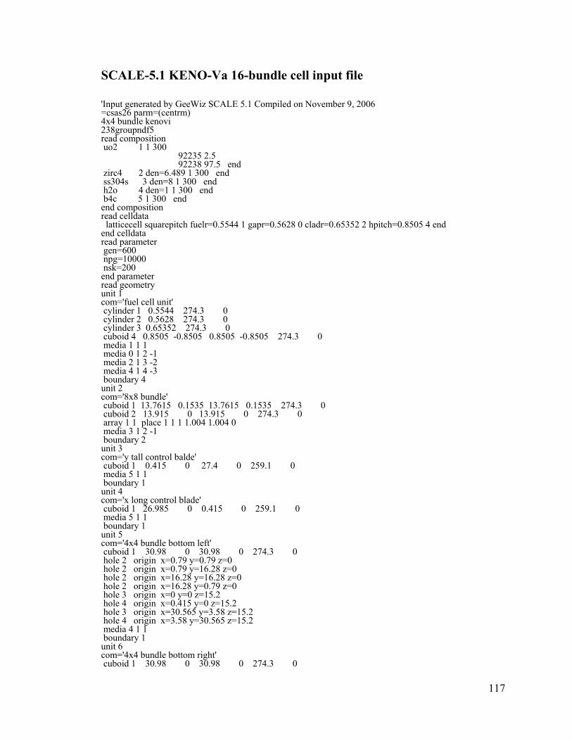
117
SCALE-5.1 KENO-Va 16-bundle cell input file 'Input generated by GeeWiz SCALE 5.1 Compiled on November 9, 2006 =csas26 parm=(centrm) 4x4 bundle kenovi 238groupndf5 read composition uo2 1 1 300 92235 2.5 92238 97.5 end zirc4 2 den=6.489 1 300 end ss304s 3 den=8 1 300 end h2o 4 den=1 1 300 end b4c 5 1 300 end end composition read celldata latticecell squarepitch fuelr=0.5544 1 gapr=0.5628 0 cladr=0.65352 2 hpitch=0.8505 4 end end celldata read parameter gen=600 npg=10000 nsk=200 end parameter read geometry unit 1 com='fuel cell unit' cylinder 1 0.5544 274.3 0 cylinder 2 0.5628 274.3 0 cylinder 3 0.65352 274.3 0 cuboid 4 0.8505 -0.8505 0.8505 -0.8505 274.3 0 media 1 1 1 media 0 1 2 -1 media 2 1 3 -2 media 4 1 4 -3 boundary 4 unit 2 com='8x8 bundle' cuboid 1 13.7615 0.1535 13.7615 0.1535 274.3 0 cuboid 2 13.915 0 13.915 0 274.3 0 array 1 1 place 1 1 1 1.004 1.004 0 media 3 1 2 -1 boundary 2 unit 3 com='y tall control balde' cuboid 1 0.415 0 27.4 0 259.1 0 media 5 1 1 boundary 1 unit 4 com='x long control blade' cuboid 1 26.985 0 0.415 0 259.1 0 media 5 1 1 boundary 1 unit 5 com='4x4 bundle bottom left' cuboid 1 30.98 0 30.98 0 274.3 0 hole 2 origin x=0.79 y=0.79 z=0 hole 2 origin x=0.79 y=16.28 z=0 hole 2 origin x=16.28 y=16.28 z=0 hole 2 origin x=16.28 y=0.79 z=0 hole 3 origin x=0 y=0 z=15.2 hole 4 origin x=0.415 y=0 z=15.2 hole 3 origin x=30.565 y=3.58 z=15.2 hole 4 origin x=3.58 y=30.565 z=15.2 media 4 1 1 boundary 1 unit 6 com='4x4 bundle bottom right' cuboid 1 30.98 0 30.98 0 274.3 0
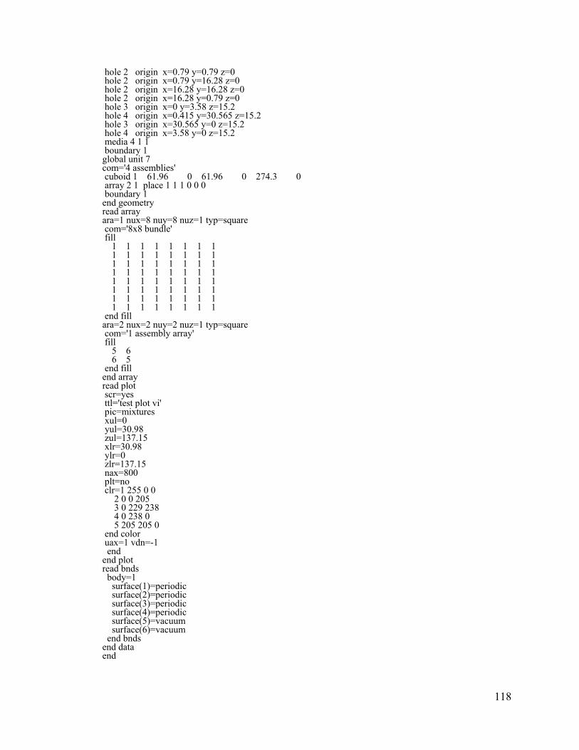
118
hole 2 origin x=0.79 y=0.79 z=0 hole 2 origin x=0.79 y=16.28 z=0 hole 2 origin x=16.28 y=16.28 z=0 hole 2 origin x=16.28 y=0.79 z=0 hole 3 origin x=0 y=3.58 z=15.2 hole 4 origin x=0.415 y=30.565 z=15.2 hole 3 origin x=30.565 y=0 z=15.2 hole 4 origin x=3.58 y=0 z=15.2 media 4 1 1 boundary 1 global unit 7 com='4 assemblies' cuboid 1 61.96 0 61.96 0 274.3 0 array 2 1 place 1 1 1 0 0 0 boundary 1 end geometry read array ara=1 nux=8 nuy=8 nuz=1 typ=square com='8x8 bundle' fill 1 1 1 1 1 1 1 1 1 1 1 1 1 1 1 1 1 1 1 1 1 1 1 1 1 1 1 1 1 1 1 1 1 1 1 1 1 1 1 1 1 1 1 1 1 1 1 1 1 1 1 1 1 1 1 1 1 1 1 1 1 1 1 1 end fill ara=2 nux=2 nuy=2 nuz=1 typ=square com='1 assembly array' fill 5 6 6 5 end fill end array read plot scr=yes ttl='test plot vi' pic=mixtures xul=0 yul=30.98 zul=137.15 xlr=30.98 ylr=0 zlr=137.15 nax=800 plt=no clr=1 255 0 0 2 0 0 205 3 0 229 238 4 0 238 0 5 205 205 0 end color uax=1 vdn=-1 end end plot read bnds body=1 surface(1)=periodic surface(2)=periodic surface(3)=periodic surface(4)=periodic surface(5)=vacuum surface(6)=vacuum end bnds end data end
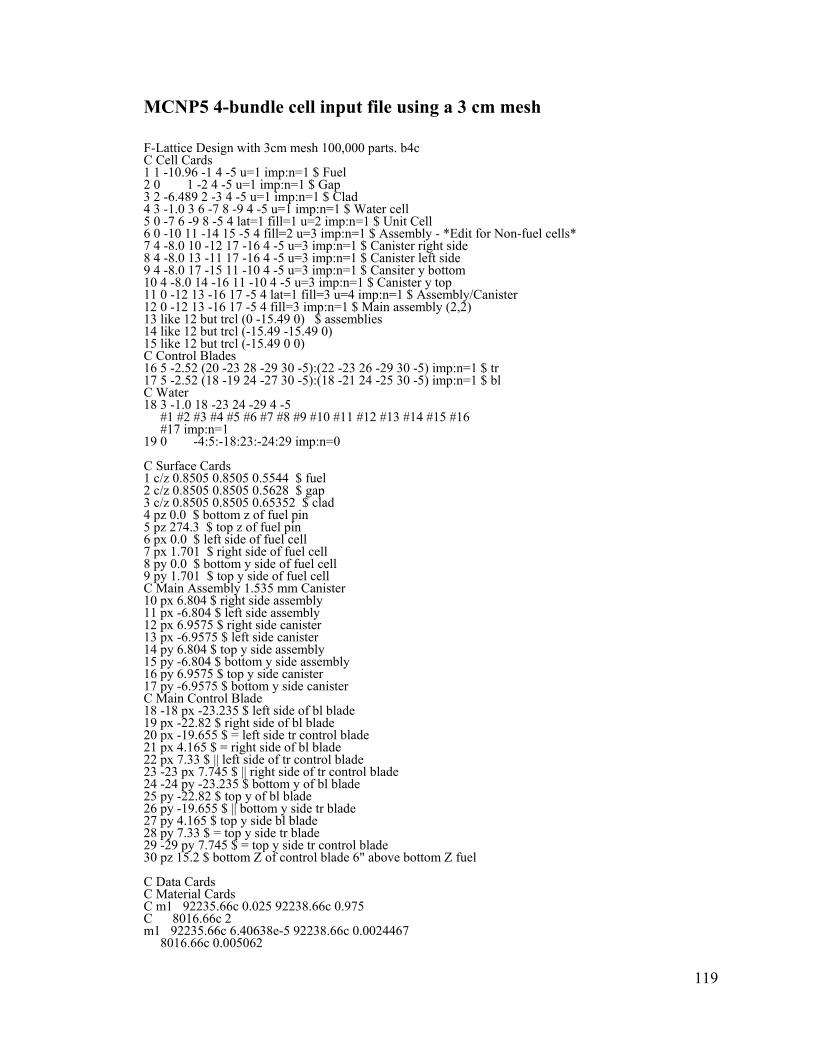
119
MCNP5 4-bundle cell input file using a 3 cm mesh F-Lattice Design with 3cm mesh 100,000 parts. b4c C Cell Cards 1 1 -10.96 -1 4 -5 u=1 imp:n=1 $ Fuel 2 0 1 -2 4 -5 u=1 imp:n=1 $ Gap 3 2 -6.489 2 -3 4 -5 u=1 imp:n=1 $ Clad 4 3 -1.0 3 6 -7 8 -9 4 -5 u=1 imp:n=1 $ Water cell 5 0 -7 6 -9 8 -5 4 lat=1 fill=1 u=2 imp:n=1 $ Unit Cell 6 0 -10 11 -14 15 -5 4 fill=2 u=3 imp:n=1 $ Assembly - *Edit for Non-fuel cells* 7 4 -8.0 10 -12 17 -16 4 -5 u=3 imp:n=1 $ Canister right side 8 4 -8.0 13 -11 17 -16 4 -5 u=3 imp:n=1 $ Canister left side 9 4 -8.0 17 -15 11 -10 4 -5 u=3 imp:n=1 $ Cansiter y bottom 10 4 -8.0 14 -16 11 -10 4 -5 u=3 imp:n=1 $ Canister y top 11 0 -12 13 -16 17 -5 4 lat=1 fill=3 u=4 imp:n=1 $ Assembly/Canister 12 0 -12 13 -16 17 -5 4 fill=3 imp:n=1 $ Main assembly (2,2) 13 like 12 but trcl (0 -15.49 0) $ assemblies 14 like 12 but trcl (-15.49 -15.49 0) 15 like 12 but trcl (-15.49 0 0) C Control Blades 16 5 -2.52 (20 -23 28 -29 30 -5):(22 -23 26 -29 30 -5) imp:n=1 $ tr 17 5 -2.52 (18 -19 24 -27 30 -5):(18 -21 24 -25 30 -5) imp:n=1 $ bl C Water 18 3 -1.0 18 -23 24 -29 4 -5 #1 #2 #3 #4 #5 #6 #7 #8 #9 #10 #11 #12 #13 #14 #15 #16 #17 imp:n=1 19 0 -4:5:-18:23:-24:29 imp:n=0 C Surface Cards 1 c/z 0.8505 0.8505 0.5544 $ fuel 2 c/z 0.8505 0.8505 0.5628 $ gap 3 c/z 0.8505 0.8505 0.65352 $ clad 4 pz 0.0 $ bottom z of fuel pin 5 pz 274.3 $ top z of fuel pin 6 px 0.0 $ left side of fuel cell 7 px 1.701 $ right side of fuel cell 8 py 0.0 $ bottom y side of fuel cell 9 py 1.701 $ top y side of fuel cell C Main Assembly 1.535 mm Canister 10 px 6.804 $ right side assembly 11 px -6.804 $ left side assembly 12 px 6.9575 $ right side canister 13 px -6.9575 $ left side canister 14 py 6.804 $ top y side assembly 15 py -6.804 $ bottom y side assembly 16 py 6.9575 $ top y side canister 17 py -6.9575 $ bottom y side canister C Main Control Blade 18 -18 px -23.235 $ left side of bl blade 19 px -22.82 $ right side of bl blade 20 px -19.655 $ = left side tr control blade 21 px 4.165 $ = right side of bl blade 22 px 7.33 $ || left side of tr control blade 23 -23 px 7.745 $ || right side of tr control blade 24 -24 py -23.235 $ bottom y of bl blade 25 py -22.82 $ top y of bl blade 26 py -19.655 $ || bottom y side tr blade 27 py 4.165 $ top y side bl blade 28 py 7.33 $ = top y side tr blade 29 -29 py 7.745 $ = top y side tr control blade 30 pz 15.2 $ bottom Z of control blade 6" above bottom Z fuel C Data Cards C Material Cards C m1 92235.66c 0.025 92238.66c 0.975 C 8016.66c 2 m1 92235.66c 6.40638e-5 92238.66c 0.0024467 8016.66c 0.005062
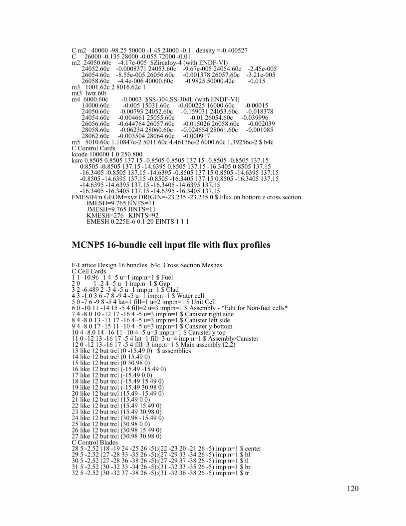
120
C m2 40000 -98.25 50000 -1.45 24000 -0.1 density =-0.400527 C 26000 -0.135 28000 -0.055 72000 -0.01 m2 24050.60c -4.17e-005 $Zircaloy-4 (with ENDF-VI) 24052.60c -0.0008371 24053.60c -9.67e-005 24054.60c -2.45e-005 26054.60c -8.55e-005 26056.60c -0.001378 26057.60c -3.21e-005 26058.60c -4.4e-006 40000.60c -0.9825 50000.42c -0.015 m3 1001.62c 2 8016.62c 1 mt3 lwtr.60t m4 6000.60c -0.0003 $SS-304,SS-304L (with ENDF-VI) 14000.60c -0.005 15031.60c -0.000225 16000.60c -0.00015 24050.60c -0.00793 24052.60c -0.159031 24053.60c -0.018378 24054.60c -0.004661 25055.60c -0.01 26054.60c -0.039996 26056.60c -0.644764 26057.60c -0.015026 26058.60c -0.002039 28058.60c -0.06234 28060.60c -0.024654 28061.60c -0.001085 28062.60c -0.003504 28064.60c -0.000917 m5 5010.60c 1.10847e-2 5011.60c 4.46176e-2 6000.60c 1.39256e-2 $ b4c C Control Cards kcode 100000 1.0 250 800 ksrc 0.8505 0.8505 137.15 -0.8505 0.8505 137.15 -0.8505 -0.8505 137.15 0.8505 -0.8505 137.15 -14.6395 0.8505 137.15 -16.3405 0.8505 137.15 -16.3405 -0.8505 137.15 -14.6395 -0.8505 137.15 0.8505 -14.6395 137.15 -0.8505 -14.6395 137.15 -0.8505 -16.3405 137.15 0.8505 -16.3405 137.15 -14.6395 -14.6395 137.15 -16.3405 -14.6395 137.15 -16.3405 -16.3405 137.15 -14.6395 -16.3405 137.15 FMESH4:n GEOM=xyz ORIGIN=-23.235 -23.235 0 $ Flux on bottom z cross section IMESH=9.765 IINTS=11 JMESH=9.765 JINTS=11 KMESH=276 KINTS=92 EMESH 0.225E-6 0.1 20 EINTS 1 1 1
MCNP5 16-bundle cell input file with flux profiles F-Lattice Design 16 bundles. b4c. Cross Section Meshes C Cell Cards 1 1 -10.96 -1 4 -5 u=1 imp:n=1 $ Fuel 2 0 1 -2 4 -5 u=1 imp:n=1 $ Gap 3 2 -6.489 2 -3 4 -5 u=1 imp:n=1 $ Clad 4 3 -1.0 3 6 -7 8 -9 4 -5 u=1 imp:n=1 $ Water cell 5 0 -7 6 -9 8 -5 4 lat=1 fill=1 u=2 imp:n=1 $ Unit Cell 6 0 -10 11 -14 15 -5 4 fill=2 u=3 imp:n=1 $ Assembly - *Edit for Non-fuel cells* 7 4 -8.0 10 -12 17 -16 4 -5 u=3 imp:n=1 $ Canister right side 8 4 -8.0 13 -11 17 -16 4 -5 u=3 imp:n=1 $ Canister left side 9 4 -8.0 17 -15 11 -10 4 -5 u=3 imp:n=1 $ Cansiter y bottom 10 4 -8.0 14 -16 11 -10 4 -5 u=3 imp:n=1 $ Canister y top 11 0 -12 13 -16 17 -5 4 lat=1 fill=3 u=4 imp:n=1 $ Assembly/Canister 12 0 -12 13 -16 17 -5 4 fill=3 imp:n=1 $ Main assembly (2,2) 13 like 12 but trcl (0 -15.49 0) $ assemblies 14 like 12 but trcl (0 15.49 0) 15 like 12 but trcl (0 30.98 0) 16 like 12 but trcl (-15.49 -15.49 0) 17 like 12 but trcl (-15.49 0 0) 18 like 12 but trcl (-15.49 15.49 0) 19 like 12 but trcl (-15.49 30.98 0) 20 like 12 but trcl (15.49 -15.49 0) 21 like 12 but trcl (15.49 0 0) 22 like 12 but trcl (15.49 15.49 0) 23 like 12 but trcl (15.49 30.98 0) 24 like 12 but trcl (30.98 -15.49 0) 25 like 12 but trcl (30.98 0 0) 26 like 12 but trcl (30.98 15.49 0) 27 like 12 but trcl (30.98 30.98 0) C Control Blades 28 5 -2.52 (18 -19 24 -25 26 -5):(22 -23 20 -21 26 -5) imp:n=1 $ center 29 5 -2.52 (27 -28 33 -35 26 -5):(27 -29 33 -34 26 -5) imp:n=1 $ bl 30 5 -2.52 (27 -28 36 -38 26 -5):(27 -29 37 -38 26 -5) imp:n=1 $ tl 31 5 -2.52 (30 -32 33 -34 26 -5):(31 -32 33 -35 26 -5) imp:n=1 $ br 32 5 -2.52 (30 -32 37 -38 26 -5):(31 -32 36 -38 26 -5) imp:n=1 $ tr
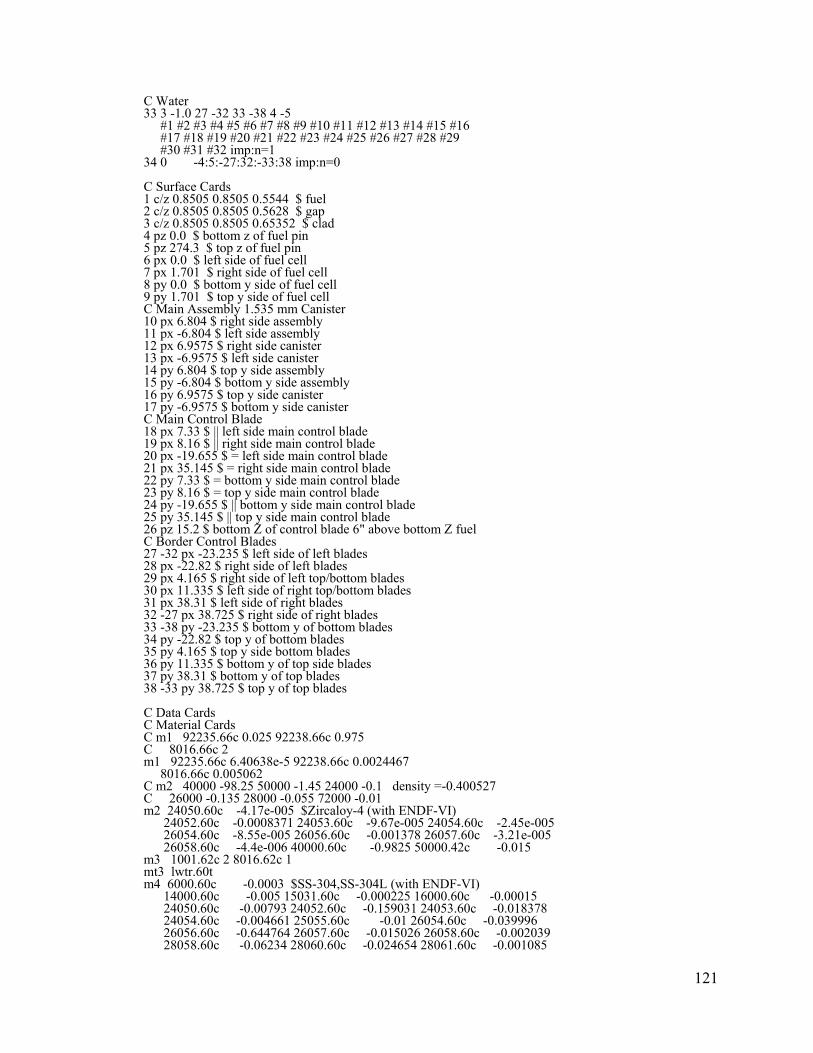
121
C Water 33 3 -1.0 27 -32 33 -38 4 -5 #1 #2 #3 #4 #5 #6 #7 #8 #9 #10 #11 #12 #13 #14 #15 #16 #17 #18 #19 #20 #21 #22 #23 #24 #25 #26 #27 #28 #29 #30 #31 #32 imp:n=1 34 0 -4:5:-27:32:-33:38 imp:n=0 C Surface Cards 1 c/z 0.8505 0.8505 0.5544 $ fuel 2 c/z 0.8505 0.8505 0.5628 $ gap 3 c/z 0.8505 0.8505 0.65352 $ clad 4 pz 0.0 $ bottom z of fuel pin 5 pz 274.3 $ top z of fuel pin 6 px 0.0 $ left side of fuel cell 7 px 1.701 $ right side of fuel cell 8 py 0.0 $ bottom y side of fuel cell 9 py 1.701 $ top y side of fuel cell C Main Assembly 1.535 mm Canister 10 px 6.804 $ right side assembly 11 px -6.804 $ left side assembly 12 px 6.9575 $ right side canister 13 px -6.9575 $ left side canister 14 py 6.804 $ top y side assembly 15 py -6.804 $ bottom y side assembly 16 py 6.9575 $ top y side canister 17 py -6.9575 $ bottom y side canister C Main Control Blade 18 px 7.33 $ || left side main control blade 19 px 8.16 $ || right side main control blade 20 px -19.655 $ = left side main control blade 21 px 35.145 $ = right side main control blade 22 py 7.33 $ = bottom y side main control blade 23 py 8.16 $ = top y side main control blade 24 py -19.655 $ || bottom y side main control blade 25 py 35.145 $ || top y side main control blade 26 pz 15.2 $ bottom Z of control blade 6" above bottom Z fuel C Border Control Blades 27 -32 px -23.235 $ left side of left blades 28 px -22.82 $ right side of left blades 29 px 4.165 $ right side of left top/bottom blades 30 px 11.335 $ left side of right top/bottom blades 31 px 38.31 $ left side of right blades 32 -27 px 38.725 $ right side of right blades 33 -38 py -23.235 $ bottom y of bottom blades 34 py -22.82 $ top y of bottom blades 35 py 4.165 $ top y side bottom blades 36 py 11.335 $ bottom y of top side blades 37 py 38.31 $ bottom y of top blades 38 -33 py 38.725 $ top y of top blades C Data Cards C Material Cards C m1 92235.66c 0.025 92238.66c 0.975 C 8016.66c 2 m1 92235.66c 6.40638e-5 92238.66c 0.0024467 8016.66c 0.005062 C m2 40000 -98.25 50000 -1.45 24000 -0.1 density =-0.400527 C 26000 -0.135 28000 -0.055 72000 -0.01 m2 24050.60c -4.17e-005 $Zircaloy-4 (with ENDF-VI) 24052.60c -0.0008371 24053.60c -9.67e-005 24054.60c -2.45e-005 26054.60c -8.55e-005 26056.60c -0.001378 26057.60c -3.21e-005 26058.60c -4.4e-006 40000.60c -0.9825 50000.42c -0.015 m3 1001.62c 2 8016.62c 1 mt3 lwtr.60t m4 6000.60c -0.0003 $SS-304,SS-304L (with ENDF-VI) 14000.60c -0.005 15031.60c -0.000225 16000.60c -0.00015 24050.60c -0.00793 24052.60c -0.159031 24053.60c -0.018378 24054.60c -0.004661 25055.60c -0.01 26054.60c -0.039996 26056.60c -0.644764 26057.60c -0.015026 26058.60c -0.002039 28058.60c -0.06234 28060.60c -0.024654 28061.60c -0.001085
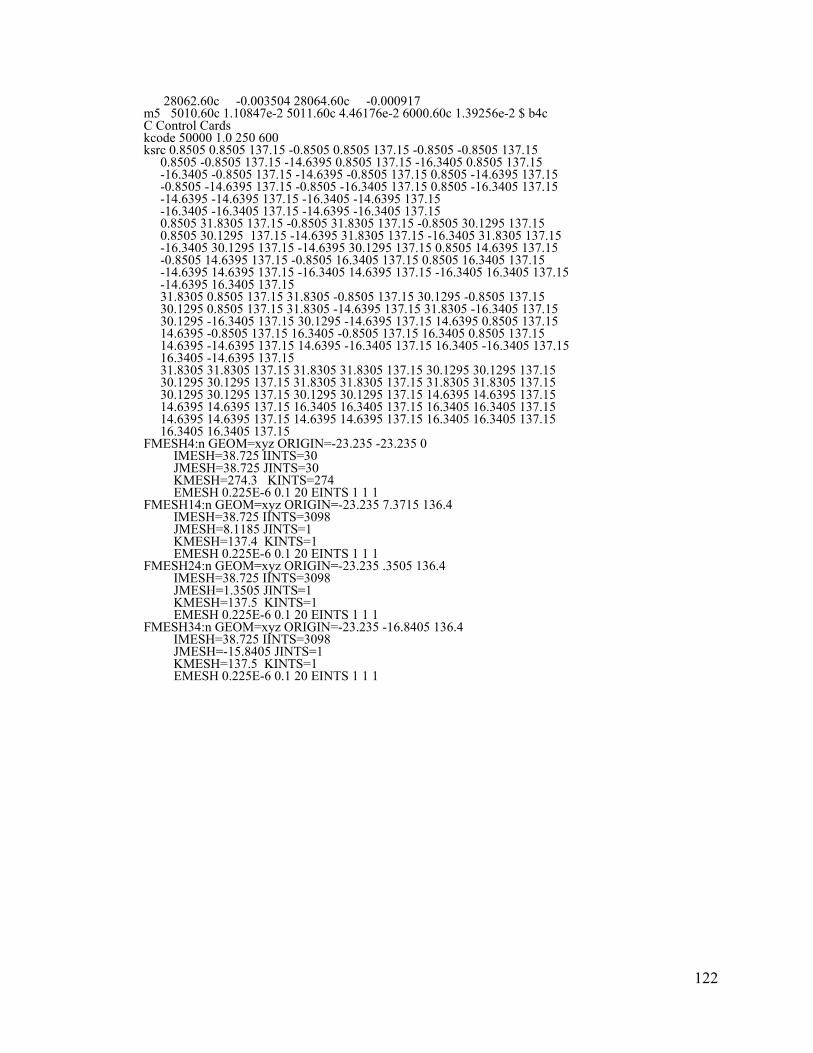
122
28062.60c -0.003504 28064.60c -0.000917 m5 5010.60c 1.10847e-2 5011.60c 4.46176e-2 6000.60c 1.39256e-2 $ b4c C Control Cards kcode 50000 1.0 250 600 ksrc 0.8505 0.8505 137.15 -0.8505 0.8505 137.15 -0.8505 -0.8505 137.15 0.8505 -0.8505 137.15 -14.6395 0.8505 137.15 -16.3405 0.8505 137.15 -16.3405 -0.8505 137.15 -14.6395 -0.8505 137.15 0.8505 -14.6395 137.15 -0.8505 -14.6395 137.15 -0.8505 -16.3405 137.15 0.8505 -16.3405 137.15 -14.6395 -14.6395 137.15 -16.3405 -14.6395 137.15 -16.3405 -16.3405 137.15 -14.6395 -16.3405 137.15 0.8505 31.8305 137.15 -0.8505 31.8305 137.15 -0.8505 30.1295 137.15 0.8505 30.1295 137.15 -14.6395 31.8305 137.15 -16.3405 31.8305 137.15 -16.3405 30.1295 137.15 -14.6395 30.1295 137.15 0.8505 14.6395 137.15 -0.8505 14.6395 137.15 -0.8505 16.3405 137.15 0.8505 16.3405 137.15 -14.6395 14.6395 137.15 -16.3405 14.6395 137.15 -16.3405 16.3405 137.15 -14.6395 16.3405 137.15 31.8305 0.8505 137.15 31.8305 -0.8505 137.15 30.1295 -0.8505 137.15 30.1295 0.8505 137.15 31.8305 -14.6395 137.15 31.8305 -16.3405 137.15 30.1295 -16.3405 137.15 30.1295 -14.6395 137.15 14.6395 0.8505 137.15 14.6395 -0.8505 137.15 16.3405 -0.8505 137.15 16.3405 0.8505 137.15 14.6395 -14.6395 137.15 14.6395 -16.3405 137.15 16.3405 -16.3405 137.15 16.3405 -14.6395 137.15 31.8305 31.8305 137.15 31.8305 31.8305 137.15 30.1295 30.1295 137.15 30.1295 30.1295 137.15 31.8305 31.8305 137.15 31.8305 31.8305 137.15 30.1295 30.1295 137.15 30.1295 30.1295 137.15 14.6395 14.6395 137.15 14.6395 14.6395 137.15 16.3405 16.3405 137.15 16.3405 16.3405 137.15 14.6395 14.6395 137.15 14.6395 14.6395 137.15 16.3405 16.3405 137.15 16.3405 16.3405 137.15 FMESH4:n GEOM=xyz ORIGIN=-23.235 -23.235 0 IMESH=38.725 IINTS=30 JMESH=38.725 JINTS=30 KMESH=274.3 KINTS=274 EMESH 0.225E-6 0.1 20 EINTS 1 1 1 FMESH14:n GEOM=xyz ORIGIN=-23.235 7.3715 136.4 IMESH=38.725 IINTS=3098 JMESH=8.1185 JINTS=1 KMESH=137.4 KINTS=1 EMESH 0.225E-6 0.1 20 EINTS 1 1 1 FMESH24:n GEOM=xyz ORIGIN=-23.235 .3505 136.4 IMESH=38.725 IINTS=3098 JMESH=1.3505 JINTS=1 KMESH=137.5 KINTS=1 EMESH 0.225E-6 0.1 20 EINTS 1 1 1 FMESH34:n GEOM=xyz ORIGIN=-23.235 -16.8405 136.4 IMESH=38.725 IINTS=3098 JMESH=-15.8405 JINTS=1 KMESH=137.5 KINTS=1 EMESH 0.225E-6 0.1 20 EINTS 1 1 1
123
Appendix C: FluxParse.pl
FluxParse.pl is a Perl script that operates on SCALE-5/KENO-Va output files
containing superimposed mesh flux results. Flux results are organized to a per cell basis
and reported in Flux.txt normalized to “per starting particle.” A “volume averaging”
error is present because only the model’s total unit volume and total cell occurrences are
reported. Individual cell “region volumes” are required to eliminate this error.
The DOS command to run this code, while in the same directory as the output
file, is:
: > FluxParse.pl ScaleOutpitName.out
FluxParse.pl Script #!/usr/bin/perl -w # Steven Weiss # FluxParse.pl # This data will find, organize and add up the fluxes for each location # produced from a Scale5 - KenoV.a output for arbitrary Mesh Size in the # x,y and z dimensions # Output will be a tab delimited text file (Flux.txt) that can be easily # converted into an Excel Worksheet format. # Command Line: > FluxParse.pl ScaleOutputName.out # Make sure to have both files in the same directory or to correctly reference # location. Output will be to current directory ($scale_file) = @ARGV; open(SCALE, $scale_file) or die "Cannot open $!"; @flux=[ [ [ ] ] ]; #initialize 3-dimensional array @Vol=[ [ ] ]; #initialize 2-d array for volume info $xmax=0; # Used to keep track of length of each dimension $ymax=0; $zmax=0; #Volume Info Finder while (<SCALE>) { $line = $_;
124
chomp($line); @test = split (' ',$line); if (@test > 3){ if ("$test[1]" =~ "msh"){ if ("$test[2]" =~ "mesh"){ $mshVol = $test[8]*$test[8]*$test[8]; } } if ("$test[0]" =~ "sum"){ if ("$test[1]" =~ "of"){ if ("$test[2]" =~ "mesh") { $line = <SCALE>; #Skip down 4 lines from "sum of mesh $line = <SCALE>; #volumes" to Data Desired $line = <SCALE>; $line = <SCALE>; chomp($line); @volume = split (' ',$line); $volume = @volume; $temp = 1; #pre-declare for scope reasons while ($volume < 9){ if ($volume == 7){ #First region of a unit $unit = $volume[0]; $temp = $unit; $region = $volume[2]; $Tvolume = $volume[4]; $NumUsed = $volume[6]; } if ($volume == 6){ #First region of a unit no Mix # $unit = $volume[0]; $temp = $unit; $region = $volume[2]; $Tvolume = $volume[3]; $NumUsed = $volume[5]; } if ($volume == 5){ #2nd+ region of a unit $unit = $temp; $region = $volume[0]; $Tvolume = $volume[2]; $NumUsed = $volume[4]; } $Vol[$unit][$region] = $Tvolume / $NumUsed; $line = <SCALE>; @volume = split (' ',$line); $volume = @volume; } if ($volume > 8){ goto MESH } } } } } }

125
#Read output line by line searching for Mesh Fluxes MESH: while (<SCALE>) { $line = $_; chomp($line); if ("$line" =~ "Mesh Fluxes") { $line = <SCALE>; #Skip down 4 lines from "Mesh Fluxes" to Data Desired $line = <SCALE>; $line = <SCALE>; $line = <SCALE>; chomp($line); # Remove the \n or RETURN from end of line INNER: for ($count=1; $count<239; $count++) { @data = split (' ',$line); #break line into individual columns #$energy = $data[0]; $unit = $data[1]; $region = $data[2]; $xvalue = $data[3]; $yvalue = $data[4]; $zvalue = $data[5]; $value = $data[6]; #print($energy);print("\n"); #print($unit);print("\n"); #print($region);print("\n"); #print($Leth[$energy]);print("\n"); #print($Vol[$unit][$region]);print("\n"); #print($value);print("\n"); #$AddValue = (($value)*($Leth[$energy])*($Vol[$unit][$region]))/($Leth[0]); $AddValue = ($value) * ($Vol[$unit][$region])/($mshVol); #print($AddValue);print("\n"); #$AddValue = 0; $flux[$xvalue][$yvalue][$zvalue]+= $AddValue; #add up fluxes at (x,y,z) if ($xvalue > $xmax){ $xmax = $xvalue; } if ($yvalue > $ymax){ $ymax = $yvalue; } if ($zvalue > $zmax){ $zmax = $zvalue; } $line = <SCALE>; chomp($line); } $line = <SCALE>; #skip blank lines after Energy Group 238 $line = <SCALE>; chomp($line); @Size = split (' ',$line); # Here @Size > 0 implies not a blank line, meaning there is still # data for this region of the current unit # If @Size <0 then it is a blank line and code will search for the # next location of "Mesh Fluxes", ie, the next unit and region if (@Size > 0) { goto INNER } } }
126
close(SCALE); # output code in tab delimited format to be easily converted to Excel Format open(OUTPUT, ">Flux.txt"); printf OUTPUT "X Y Z Flux\n"; for($i=1; $i <= $xmax; $i++){ for($j=1; $j <= $ymax; $j++) { for($k=1; $k <= $zmax; $k++){ printf OUTPUT "$i $j $k $flux[$i][$j][$k]\n"; } } } close(OUTPUT);
Simple Test Case Verification Two simple cases were used to test the results of FluxParse.pl before it was
applied to the F-Lattice. The first test case was a homogeneous cube, 10 cm on each side,
of UO2 that is enriched to five weight percent Uranium-235. The second case tested was
the simple plate fuel reactor described in Chapter 3 for use in the computational cost
comparisons. The plate fuel geometry provides a multiple region problem, which
introduces varying “region volume” sizes (and thus the volume averaging error)
discussed in Chapter 4. The results are shown in Table C.1 and Table C.2 for the
homogeneous cube and the slab geometries respectively. Accurate results are obtained
for the average flux values; however there is some error in specific peak values due to the
volume averaging error discussed in Chapter 4. The different (x, y, z) locations for the
peak flux values in Table C.1 can be accounted for by the symmetry in the system.

127
Homogeneous Cube 1.0 cm Mesh
X Y Z Peak Flux (n/cm^2-s)
% Error Relative to MCNP
Average Flux (n/cm^2-s)
% Error Relative to MCNP
MCNP 8.5 2.5 5.5 6.8192E+18 0.00 6.6782E+18 0.00 SCALE 1.5 7.5 4.5 6.7980E+18 -0.31 6.6590E+18 -0.29 Homogeneous Cube 5.0 cm Mesh
X Y Z Peak Flux (n/cm^2-s)
% Error Relative to MCNP
Average Flux (n/cm^2-s)
% Error Relative to MCNP
MCNP 7.5 7.5 2.5 6.6880E+18 0.00 6.6782E+18 0.00 SCALE 2.5 7.5 7.5 6.6651E+18 -0.34 6.6590E+18 -0.29
Table C.1: Flux results for a simple homogeneous cube system.
Fuel plate Geometry 2 cm Mesh
X Y Z Peak Flux (n/cm^2-s)
% Error Relative to MCNP
Average Flux (n/cm^2-s)
% Error Relative to MCNP
MCNP 23 17 55 6.4046E+16 0.00 2.7132E+16 0.00 SCALE 2 7 25 8.5171E+16 32.98 2.6685E+16 -1.65 Fuel plate Geometry 5 cm Mesh
X Y Z Peak Flux (n/cm^2-s)
% Error Relative to MCNP
Average Flux (n/cm^2-s)
% Error Relative to MCNP
MCNP 22.5 17.5 57.5 5.7662E+16 0.00 2.7734E+16 0.00 SCALE 32.5 17.5 57.5 5.8576E+16 1.58 2.7132E+16 -2.17
Table C.2: Flux results for a slab geometry system.
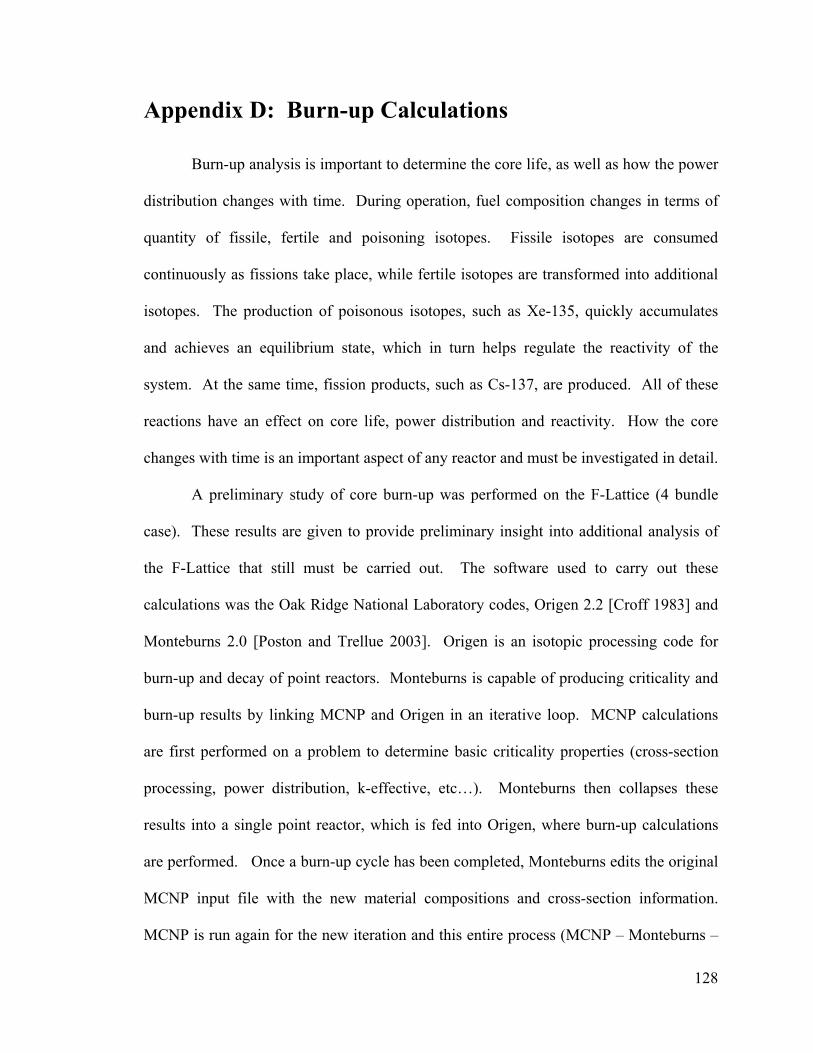
128
Appendix D: Burn-up Calculations
Burn-up analysis is important to determine the core life, as well as how the power
distribution changes with time. During operation, fuel composition changes in terms of
quantity of fissile, fertile and poisoning isotopes. Fissile isotopes are consumed
continuously as fissions take place, while fertile isotopes are transformed into additional
isotopes. The production of poisonous isotopes, such as Xe-135, quickly accumulates
and achieves an equilibrium state, which in turn helps regulate the reactivity of the
system. At the same time, fission products, such as Cs-137, are produced. All of these
reactions have an effect on core life, power distribution and reactivity. How the core
changes with time is an important aspect of any reactor and must be investigated in detail.
A preliminary study of core burn-up was performed on the F-Lattice (4 bundle
case). These results are given to provide preliminary insight into additional analysis of
the F-Lattice that still must be carried out. The software used to carry out these
calculations was the Oak Ridge National Laboratory codes, Origen 2.2 [Croff 1983] and
Monteburns 2.0 [Poston and Trellue 2003]. Origen is an isotopic processing code for
burn-up and decay of point reactors. Monteburns is capable of producing criticality and
burn-up results by linking MCNP and Origen in an iterative loop. MCNP calculations
are first performed on a problem to determine basic criticality properties (cross-section
processing, power distribution, k-effective, etc…). Monteburns then collapses these
results into a single point reactor, which is fed into Origen, where burn-up calculations
are performed. Once a burn-up cycle has been completed, Monteburns edits the original
MCNP input file with the new material compositions and cross-section information.
MCNP is run again for the new iteration and this entire process (MCNP – Monteburns –

129
Origen – Monteburns – MCNP) is repeated for the desired number of time steps. For
more information on Origen and Monteburns, refer to the documentation provided by
Croff [1983] and by Poston and Trellue [2003], respectively.
Two tests were carried out on the F-Lattice, assuming a fresh core with an
average burn rate of 9.80 MWt (control blades remain fully inserted over the entire
duration of burn). The first burn-up calculation was performed for 1 month (31 days).
Monteburns performed 31 outer burn steps (1 day intervals), which refers to the time step
in which neutron fluxes are actualized with an MCNP simulation. 60 internal steps are
performed with Origen between every out step. The Monteburns input file is included
below for more details. The second test was performed for 20 months with 40 outer steps
(2 week time steps) and 40 internal steps. K-effective calculations and important isotopic
abundances were tracked. (For a preliminary study, and due to time constraints, MCNP5
simulations were run with reduced accuracy, using only 10,000 particles for 150 inactive
cycles and 150 active cycles.)
Preliminary Burn-up Study Results The results of the 1 month burn-up calculation with 1 day time steps are given in
Figure D.1 – 7.
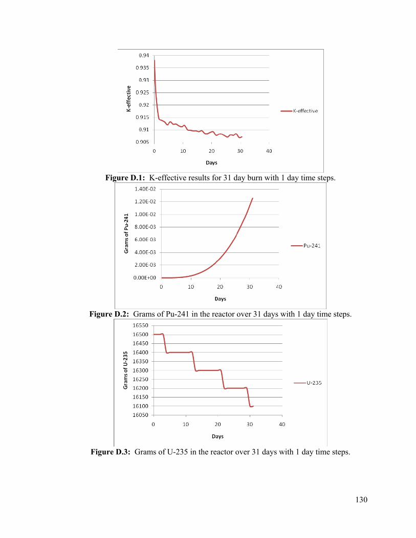
130
Figure D.1: K-effective results for 31 day burn with 1 day time steps.
Figure D.2: Grams of Pu-241 in the reactor over 31 days with 1 day time steps.
Figure D.3: Grams of U-235 in the reactor over 31 days with 1 day time steps.
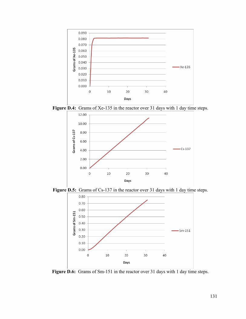
131
Figure D.4: Grams of Xe-135 in the reactor over 31 days with 1 day time steps.
Figure D.5: Grams of Cs-137 in the reactor over 31 days with 1 day time steps.
Figure D.6: Grams of Sm-151 in the reactor over 31 days with 1 day time steps.
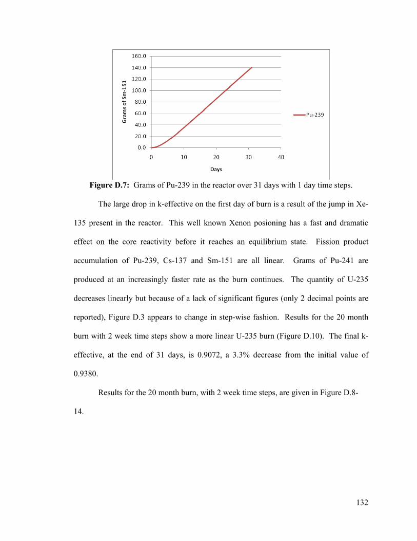
132
Figure D.7: Grams of Pu-239 in the reactor over 31 days with 1 day time steps.
The large drop in k-effective on the first day of burn is a result of the jump in Xe-
135 present in the reactor. This well known Xenon posioning has a fast and dramatic
effect on the core reactivity before it reaches an equilibrium state. Fission product
accumulation of Pu-239, Cs-137 and Sm-151 are all linear. Grams of Pu-241 are
produced at an increasingly faster rate as the burn continues. The quantity of U-235
decreases linearly but because of a lack of significant figures (only 2 decimal points are
reported), Figure D.3 appears to change in step-wise fashion. Results for the 20 month
burn with 2 week time steps show a more linear U-235 burn (Figure D.10). The final k-
effective, at the end of 31 days, is 0.9072, a 3.3% decrease from the initial value of
0.9380.
Results for the 20 month burn, with 2 week time steps, are given in Figure D.8- 14.
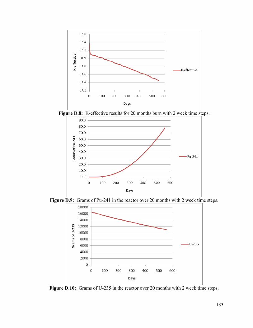
133
Figure D.8: K-effective results for 20 months burn with 2 week time steps.
Figure D.9: Grams of Pu-241 in the reactor over 20 months with 2 week time steps.
Figure D.10: Grams of U-235 in the reactor over 20 months with 2 week time steps.
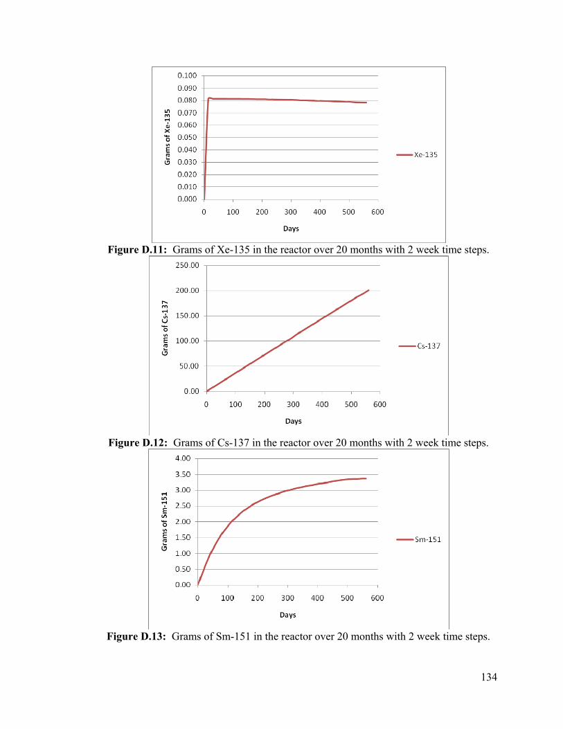
134
Figure D.11: Grams of Xe-135 in the reactor over 20 months with 2 week time steps.
Figure D.12: Grams of Cs-137 in the reactor over 20 months with 2 week time steps.
Figure D.13: Grams of Sm-151 in the reactor over 20 months with 2 week time steps.
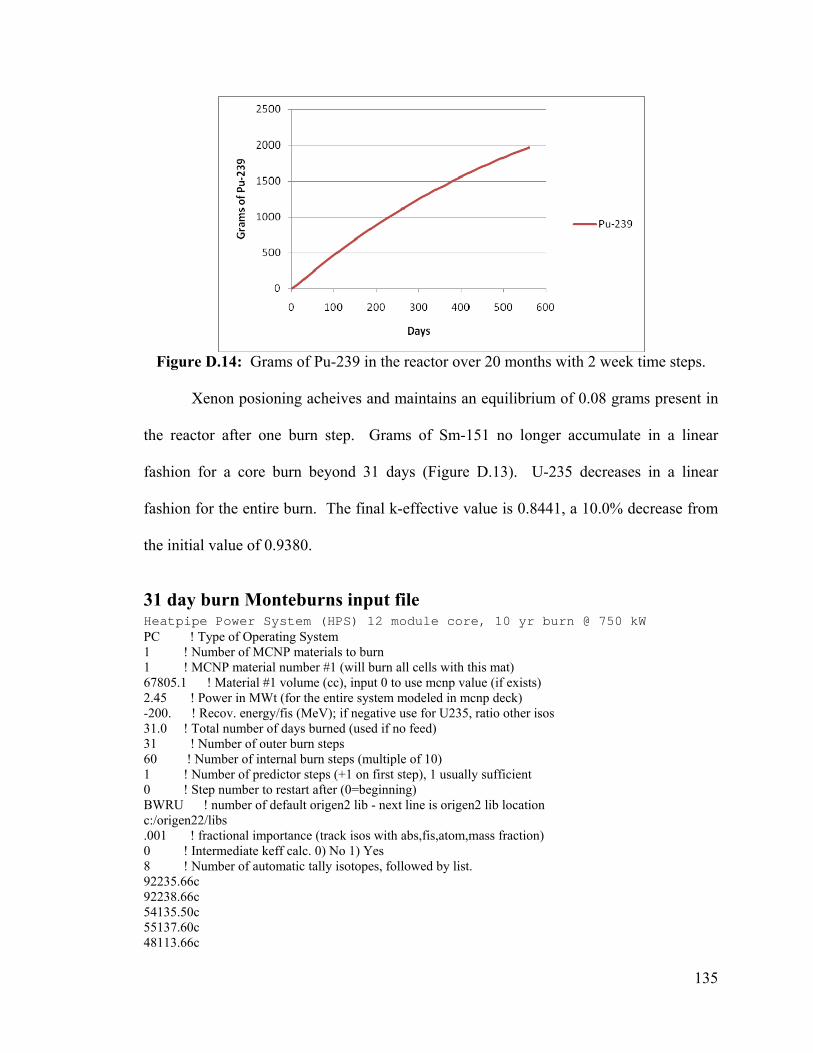
135
Figure D.14: Grams of Pu-239 in the reactor over 20 months with 2 week time steps.
Xenon posioning acheives and maintains an equilibrium of 0.08 grams present in
the reactor after one burn step. Grams of Sm-151 no longer accumulate in a linear
fashion for a core burn beyond 31 days (Figure D.13). U-235 decreases in a linear
fashion for the entire burn. The final k-effective value is 0.8441, a 10.0% decrease from
the initial value of 0.9380.
31 day burn Monteburns input file Heatpipe Power System (HPS) 12 module core, 10 yr burn @ 750 kW PC ! Type of Operating System 1 ! Number of MCNP materials to burn 1 ! MCNP material number #1 (will burn all cells with this mat) 67805.1 ! Material #1 volume (cc), input 0 to use mcnp value (if exists) 2.45 ! Power in MWt (for the entire system modeled in mcnp deck) -200. ! Recov. energy/fis (MeV); if negative use for U235, ratio other isos 31.0 ! Total number of days burned (used if no feed) 31 ! Number of outer burn steps 60 ! Number of internal burn steps (multiple of 10) 1 ! Number of predictor steps (+1 on first step), 1 usually sufficient 0 ! Step number to restart after (0=beginning) BWRU ! number of default origen2 lib - next line is origen2 lib location c:/origen22/libs .001 ! fractional importance (track isos with abs,fis,atom,mass fraction) 0 ! Intermediate keff calc. 0) No 1) Yes 8 ! Number of automatic tally isotopes, followed by list. 92235.66c 92238.66c 54135.50c 55137.60c 48113.66c
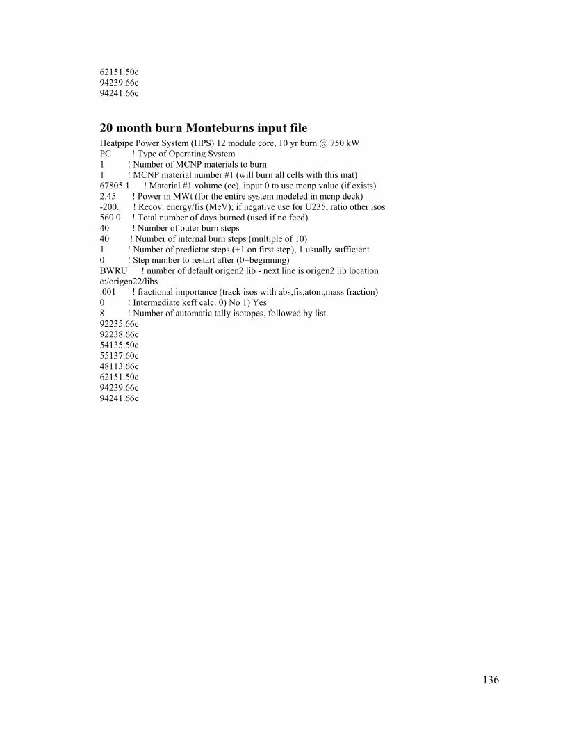
136
62151.50c 94239.66c 94241.66c
20 month burn Monteburns input file Heatpipe Power System (HPS) 12 module core, 10 yr burn @ 750 kW PC ! Type of Operating System 1 ! Number of MCNP materials to burn 1 ! MCNP material number #1 (will burn all cells with this mat) 67805.1 ! Material #1 volume (cc), input 0 to use mcnp value (if exists) 2.45 ! Power in MWt (for the entire system modeled in mcnp deck) -200. ! Recov. energy/fis (MeV); if negative use for U235, ratio other isos 560.0 ! Total number of days burned (used if no feed) 40 ! Number of outer burn steps 40 ! Number of internal burn steps (multiple of 10) 1 ! Number of predictor steps (+1 on first step), 1 usually sufficient 0 ! Step number to restart after (0=beginning) BWRU ! number of default origen2 lib - next line is origen2 lib location c:/origen22/libs .001 ! fractional importance (track isos with abs,fis,atom,mass fraction) 0 ! Intermediate keff calc. 0) No 1) Yes 8 ! Number of automatic tally isotopes, followed by list. 92235.66c 92238.66c 54135.50c 55137.60c 48113.66c 62151.50c 94239.66c 94241.66c

137
Author’s Biography
Steven Weiss was born in Oak Park, Illinois on June 20th, 1985. He graduated
from Downers Grove South High School in the spring of 2003. In the fall of 2003 he
began his studies at the University of Illinois at Urbana-Champaign. In the summer of
2005, Steven took part in a study abroad program with the Hiroshima Institute of
Technology in Hiroshima, Japan. In the spring of 2007 he graduated with a Bachelors of
Science in nuclear engineering and minor in computer science and immediately began
graduate school at the University of Illinois. Following the completion of this thesis,
Steven will be joining Westinghouse Electric Company as a Nuclear Core Design
Engineer, starting in the summer of 2008.


![Analytical solution to transient heat conduction in polar …verl.npre.illinois.edu/Documents/J-08-01.pdf · 2010-03-01 · with multiple layers in radial direction ... [1–4] in](https://img.pdfslide.us/doc/110x75/5b815dc57f8b9ae87c8c1fc7/analytical-solution-to-transient-heat-conduction-in-polar-verlnpre-2010-03-01.jpg)