Partial Online Cycle Elimination in Inclusion Constraint Graphs

Partial Online Cycle Elimination in Inclusion Constraint Graphs

Manuel FBhndrich* Jeffrey S. Foster* Zhendong Su* Alexander Aiken*

EECS Department University of California, Berkeley

387 Soda Hall #1776 Berkeley, CA 94720-1776

{manuel,jfoster,zhendong,aiken}@cs.berkeley.edu

Abstract

Many program analyses are naturally formulated and implemented using inclusion constraints. We present new results on the scalable implementation of such analyses based on two insights: first, that online elimination of cyclic constraints yields orders-of-magnitude improvements in analysis time for large problems; second, that the choice of constraint representation affects the quality and efficiency of online cycle elimination. We present an analytical model that explains our design choices and show that the model’s predictions match well with results from a substantial experiment.

1 Introduction

Inclusion constraints are a natural vehicle for expressing a wide range of program analyses including shape analysis, closure analysis, soft typing systems, receiver-class predic- tion for object-oriented programs, and points-to analysis for pointer-based programs, among others [Rey69, JM79, Shi88, PS91, AWL94, Hei94, And94, FFK+96, MW97]. Such analyses are efficient for small to medium size programs, but they are known to be impractical for large analysis problems.

Inclusion constraint systems have natural graph representations. For example, the constraints X 2 y 5 2 are represented by nodes for the quantities X,Y, and 2 and directed edges (X, Y) and (Y, 2) for the inclusions. Resolv- ing the constraints corresponds to adding new edges to the graph to express relationships implied by, but not explicit in, the initial system. In this example, the transitive edge (X, 2) represents the implied constraint X C 2.

The performance of constraint resolution can be im- proved by simplifying the constraint graph. Periodic simplification performed during resolution helps to scale to larger analysis problems [FA96, FF97, MWS’I], but performance is still unsatisfactory. One problem is deciding the frequency at which to perform simplifications to keep a well-balanced cost-benefit tradeoff. Simplification frequencies in past ap-

*Supported in part by an NDSEG fellowship, NSF Young Inves- tigator Award CCR-9457812, NSF Grant CCR-9416973, and a gift from Rockwell Corporation.

Psrmisaion lo make digital or hard copies of aII or part of this work for personal or classroom we is granted without fee provided that copies are not made or distributed for profit or commercial sdvan- tape and that copies bear this notice end the lull citation on the firs1 page. To copy otherwiss. lo republish, to post on servera or lo rsdistribute to lists. requires prior specific permission and/or a fee. SIGPLAN ‘98 Montrssl. Canada Q 1998 ACM 0-89791~987-4/98/0006...$5.00

proaches range from once for an entire module to once for every program expression.

In this paper we show that cycle elimination in the constraint graph (a particular simplification) is one key to making inclusion constraint analyses scale to large problems with good performance. Cyclic constraints have the form Xl c x2 E x3 . . . C X,, C_ Xr where the Xi are set variables. All variables on such a cycle are equal in all solutions of the constraints, and thus the cycle can be collapsed to a single variable.

We take an extreme approach to simplification frequency by performing cycle detection and elimination online, i.e., at every update of the constraint graph. At first glance, this approach seems overly expensive, since the best known algorithm for online cycle detection performs a full depth- first search for half of all edge additions [Shm83].

Our contribution is to show that partial online cycle detection can be performed cheaply by traversing only cer- tain paths during the search for cycles. This approach is inspired by a non-standard graph representation called inductive form (IF) introduced in [AWSS]. In practice, our approach requires constant time overhead on every edge addition and finds and eliminates about 80% of all variables involved in cycles. For our benchmarks, this approach radi- cally improves the scaling behavior, making analysis of large programs practical. Furthermore, we provide an analytical model to explain the performance of particular graph representations.

Except ours, all implementations of inclusion constraint solvers we are aware of employ a standard graph representation in which all edges are stored in adjacency lists and variable-variable edges always appear in successor lists. For example, the constraint X E y, between variables X and Y, is represented as a successor edge from node X to node y. Our measurements show that this standard form (SF), which is the one described in [Hei92] for use in set-based analysis (SBA), can also substantially benefit from partial online cycle elimination.

As our benchmark we study a points-to analysis for C [And94, SH97] implemented using both SF and IF. For large programs (more than 10000 lines), online cycle elimination reduces the execution time of our SF implementation by up to a factor of 13. Our implementation using IF and partial online cycle elimination outperforms SF with cycle elimination by up to a factor of 4, resulting in an overall speedup over standard implementations by up to 50.

Our measurement methodology uses a single well- engineered constraint solver to perform a number of exper-

85

iments using SF and IF with and without cycle elimination. We validate our results by comparing with Shapiro and Hor- witz’s SF implementation (SH) of the same points-to analysis [SH97]. Experiments show that our implementation of points-to analysis using SF without cycle elimination closely matches SH on our benchmarks.

In Section 2, we define a language for set constraints, the particular constraint formalism we shall use. We also present the graph representations SF and IF and describe our cycle elimination algorithm. In Section 3 we describe the version of points-to analysis we study. Section 4 presents measurements illustrating the efficacy of our cycle elimination algorithm. Section 5 studies an analytical model that explains why IF can outperform SF. Finally, Section 6 presents related work, and Section 7 concludes.

2 Definitions

2.1 Set Constraints

In this paper we use a small subset of the full language of set constraints [HJ90, AW92]. Constraints in our constraint language are of the form L 2 R, where L and R are set expressions. Set expressions consist of set variables X, Y, . . . from a family of variables Vars, terms constructed from n- ary constructors c E Con, an empty set 0, and a universal set 1.

L,RE se ::= X]c(sei,...,se,))O)l

Each constructor c is given a unique signature S, specifying the arity and variance of c. Intuitively, a constructor c is covatiant in an argument if the set denoted by a term c(. . .) becomes larger as the argument increases. Similarly, a constructor c is contravariant in an argument if the set denoted by a term c(. . . ) becomes smaller as the argument increases.

We define solutions to set constraints without restricting ourselves to a particular model’ for set expressions. We simply assume that each constructor c is also equipped with an interpretation &. Given a vatiable assignment A of sets to variables, set expressions are interpreted as follows2:

[X] A = A(X) [c(sel,... , se,)] A = qL(l[sel] A,. . . , [se,] A)

A solution to a system of constraints { Li C &} is a variable assignment A such that [Lil A C I[&] A for all i.

2.2 Constraint Graphs

Solving a system of constraints involves computing an explicit solved form of all solutions or of a particular solution. We study two distinct solved forms: Standard form SF represents the least solution explicitly and is commonly used for implementing SBA [Hei92]. Inductive form IF computes a representation of all solutions and is usually used with more expressive constraints and in type-based analyses [AW93, MW97]. As an aside, it is worth noting that for some analysis problems we require a representation of all solutions because no least solution exists. For the purposes of

‘Standard models are the termset model [Hei92, Kos93] or the ideal model IAW931.

2The inte&re&ion of 0 and 1 depends on the model and is not shown.

SU{XEX} w s

SU{se&l} ++ S

SU{OEse} * S

SU {c(sel,. . . ,se,) C c(se:,. . . , se’,)} +3 s u ui

1

{se& c se:} c covariant in i {sei > se:} c contravariant in i

S U {c(. . . ) s d(. . . )} ti no solution ifd#c

S U {c(. . . ) s 0) * no solution S U { 1 C 0) e no solution

S U { 1 E a!(. . . )} * no solution

Figure 1: Resolution rules R for SF and IF

comparing the two forms we shall implicitly assume throughout that with respect to the variables of interest constraint systems have least solutions.

The solved form of a constraint system is a directed graph G = (V, E) closed under a transitive closure rule, where the edges E represent atomic constraints and the vertices V axe variables, sources, and sinks. Sources are constructed terms appearing to the left of an inclusion, and sinks axe constructed terms appearing to the right of an inclusion. For the purposes of this paper, we treat 0 and 1 as constructors. A constraint is atomic if it is one of the three forms

XCY variable-variable constraint 2.; !(’ 5 source-variable constraint

. . . variable-sink constraint -

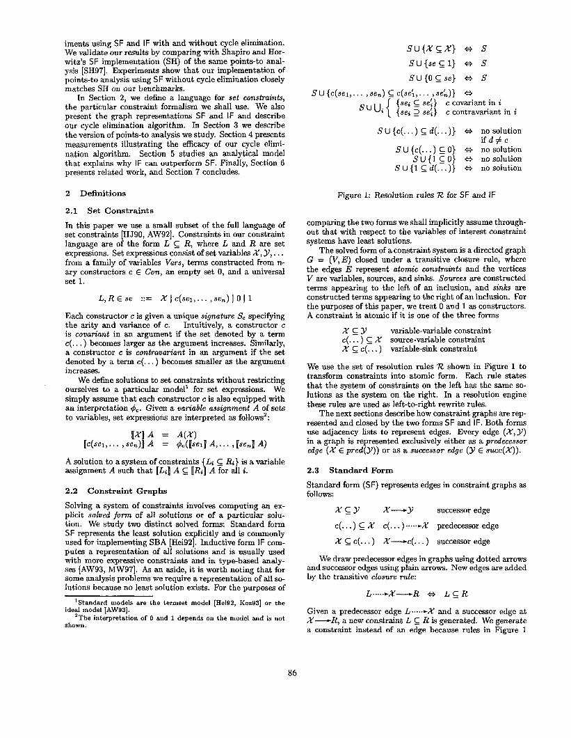
We use the set of resolution rules R shown in Figure 1 to transform constraints into atomic form. Each rule states that the system of constraints on the left has the same solutions as the system on the right. In a resolution engine these rules are used as left-to-right rewrite rules.

The next sections describe how constraint graphs are represented and closed by the two forms SF and IF. Both forms use adjacency lists to represent edges. Every edge (X,Y) in a graph is represented exclusively either as a predecessor edge (X E pred(y)) or as a successor edge (y E succ(X)).

2.3 Standard Form

Standard form (SF) represents edges in constraint graphs as follows:

XCY X-Y successor edge

c(...) G x c(...) ...+X predecessor edge

X & c(. . . ) X-c(. . . ) successor edge

We draw predecessor edges in graphs using dotted arrows and successor edges using plain arrows. New edges are added by the transitive closure rule:

L.....cX-R e LCR

Given a predecessor edge L -.-cX and a successor edge at X-R, a new constraint L c R is generated. We generate a constraint instead of an edge because rules in Figure 1

86

Lo c x i = l..k 2 g Ri i = l..m

Lk

1 Close

IF

I Close

Rl

Figure 2: Example constraints in SF and IF

may apply. Note that in this case, L is always of the form c(. . . ). This closure rule combined with rules R of Figure 1 produces a Final graph containing an explicit form of the least solution LS of the constraints [Hei92].

SF makes the least solution explicit by propagating sources forward to all reachable variables via the closure rule. The particular choice of successor and predecessor representation is motivated by the need to implement the closure rule locally. Given a variable X, the closure rule must be applied exactly to all combinations of predecessor and the successor edges of X.

Figure 2 shows an example system of constraints, the initial SF graph, and the resulting closed SF graph (left). The example assumes that set expressions L1 . . . Lk are sources and RI... R, are sinks. The closure of the standard form adds transitive edges from each source Li to all variables reachable from X i.e., Yi . . . Yt, 2. Note that the edges from Ll . . . Lk to 2 are added 1 times each, namely along all 1 edges Yi-2. The total work of closing the graph is 2kl edge additions, of which k(l - 1) additions are redundant, plus the work resulting from the km constraints Li C Rj (not shown).

To see why cycle elimination can asymptotically reduce the amount of work to close a graph, suppose there is an extra edge 2-X in Figure 2, forming a strongly connected component X, Yi , . . . , Yl, 2. If we collapse this component before adding the transitive edges Li *****+Yj, none of the 2kl transitive edge additions Li *..+Yj are performed (the km constraints Li E Rj are still produced of course).

2.4 Inductive Form

Inductive form (IF) exploits the fact that a variable-variable constraint X C Y can be represented either as a successor

edge (Y E succ(X)) or as a predecessor edge (X E Fed(Y)). The representation for a particular edge is chosen as a function of a fixed total order o : Vars + N on the variables. Edges in the constraint graph are represented as follows:

i

X-Y if o(X) > o(Y)

XCY a successor edge

X--Y if o(X) < o(Y) a predecessor edge

The choice of the order o(a) can have substantial impact on the size of the closed constraint graph and the amount of work required for the closure. We assume that the order o(-) is randomly chosen. Choosing a good order is hard, and we have found that a random order performs as well or better than any other order we picked.

The other two kinds of edges are represented as in standard form, and the closure rule also remains unchanged:

L....+X-R H L E R

Notice that L may be a source or a variable-unlike SF, where L is always a source. In IF the closure rule can therefore directly produce transitive edges between variables. (This is not to say that the closure of SF does not produce new edges between variables, but for SF such edges always involve the resolution rules R of Figure 1.) The closure rule combined with the resolution rules R produces a final graph in inductive form [AW93].

The least solution of the constraints is not explicit in the closed inductive form. However, it is easily computed as follows:

LS(Y) ={c(. . . ) 1 c(. . . ) . . ..+Y} u

87

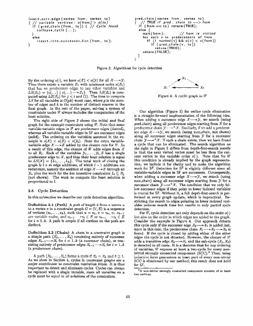
insert-succ-edge (vertex from, vertex to) { // variable vertices : o(from) > o(to)

if ( pred-chain (from, to)) { // Cycle found collapse-cycle (...);

I else

insert-into-successor-list (from, to); 1

pred-chain (vertex from, vertex to) { // TRUE if pred. chain to --> from

if (from == to) return (TRUE); else {

mark( from ); // from is visited for each v in predecessors of from

if (! marked(v) && o(v) < o(from)) if (pred-chain (v, to))

return (TRUE); return (FALSE);

1 1

Figure 3: Algorithms for cycle detection

By the ordering o(.), we have o(X) < o(Y) for all X....+Y. Thus there exists a variable 21 with minimum index o(&) that has no predecessor edges to any other variables and LS(&) = {c(. . .) [ c(. . .) . ..+Z~}. Then AS(&) is computed using LS(2j) for j < i and (1). The time to compute LS for all variables is O(pJc) worst case, where p is the number of edges and /c is the number of distinct sources in the final graph. In the rest of the paper, solving a system of constraints under IF always includes the computation of the least solution.

The right side of Figure 2 shows the initial and ha1 graph for the example constraints using IF. Note that some variable-varjable edges in IF are predecessor edges (dotted), whereas all variable-variable edges in SF are successor edges (solid). The ordering on the variables assumed in the example is o(X) < o(2) < o(yi). Note the extra variable- variable edge X *..+2 added by the closure rule for IF. As a result of this edge, the closure of IF adds edges from X to all a. Each of the variables &, . . . , Yl, 2 has a single predecessor edge to X, and thus their least solution is equal to LS(X) = {LI,... , Lk}. The total work of closing the graph is 1 + m edge additions, of which 1 - 1 additions are redundant, namely the addition of edge X....+Z through all yi, plus the work for the km transitive constraints Li 5 Rj (not shown). The work to compute the least solution is proportional to 1.

2.5 Cycle Detection

In this subsection we describe our cycle detection algorithm.

Definition 2.1 (Path) A path of length k from a vertex u to a vertex v in a constraint graph G = (V, E) is a sequence of vertices (~0 , . . . ,Vk), such that U = 210, V = ‘ok, ‘“l..Vk-1 are variable nodes, and vi-i-i E E or v~~~.~~.+~v~ E E for i = l..k. A path is simple if all vertices on the path are distinct.

Definition 2.2 (Chain) A chain in a constraint graph is a simple path (X0,. . . , xk) consisting entirely of SUCCeSSOr edges XS-~-X~ for i = l..k (a successor chain), or consisting entirely of predecessor edges Xi-1 ...++Xi for i = l..k (a predecessor chain).

A path (X0,. . . , xk) forms a cycle if X0 = Xk and k 2 1. AS we show in Section 4, cycles in constraint graphs are a major contributor to constraint resolution times. It is thus important to detect and eliminate cycles. Cycles can always be replaced with a single variable, since all variables on a cycle must be equal in all solutions of the constraints.

Figure 4: A cyclic graph in IF

Our algorithm (Figure 3) for online cycle elimination is a straight-forward implementation of the following idea. When adding a successor edge X-Y, we search (using pred-chain) along all predecessor edges starting from X for a predecessor chain JJ . . ..++X. Similarly, if we add a predecessor edge X ....+JJ, we search (using succ-chain, not shown) along all successor edges starting from Y for a successor chain y-+X. If such a chain exists, then we have found a cycle that can be eliminated. The search algorithm on the right in Figure 3 differs from depth-fist-search merely in that the next visited vertex must be less than the cur- rent vertex in the variable order o(.). Note that for IF this condition is already implied by the graph representation; we include it for clarity and to make the algorithm work for SF. Detection for SF is slightly different since all variable-variable edges in SF are successors. Consequently, when adding a successor edge X-Y, we search (using succ-chain) along all successor edges starting from Y for a successor chain y-+X. The condition that we only follow successor edges if they point to lower indexed variables is crucial for SF. Without it, a full depth-first-search is performed at every graph update, which is impractical. Re- stricting the search to edges pointing to lower indexed variables reduces search time but results in only partial cycle detection.

For IF, cycle detection not only depends on the order o(.) but also on the order in which edges are added to the graph. Consider the example in Figure 4. Our approach detects this cycle only if the successor edge X3-X1 is added last, since in this case, the predecessor chain Xl ....+Xz ...+X3 is found. If the cycle is closed by adding either of the other edges the cycle is not detected. However, the closure of IF adds a transitive edge XZ-Xl and the sub-cycle (Xl, X2) is detected in all cases. It is a theorem that for any ordering of variables, IF exposes at least a two-cycle for every non- trivial strongly connected component (SCC).3 Thus, using inductive form guarantees at least part of every non-trivial SCC is eliminated by our method; this result does not hold for SF.

‘A non-trivial strongly connected component consists of at least two vertices.

88

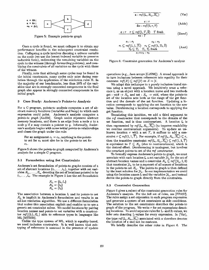
Figure 5: Example points-to graph

Once a cycle is found, we must collapse it to obtain any performance benefits in the subsequent constraint resolution. Collapsing a cycle involves choosing a witness variable on the cycle (we use the lowest indexed variable to preserve inductive form), redirecting the remaining variables on the cycle to the witness (through forwarding pointers), and com- bining the constraints of all variables on the cycle with those of the witness.

Finally, note that although some cycles may be found in the initial constraints, many cycles only arise during resolution through the application of the resolution rules R. In the majority of our benchmarks, less than 20% of the variables that are in strongly connected components in the final graph also appear in strongly connected components in the initial graph.

3 Case Study: Andersen’s Points-to Analysis

For a C program, points-to analysis computes a set of abstract memory locations (variables and heap) to which each expression could point. Andersen’s analysis computes a points-to graph [And94]. Graph nodes represent abstract memory locations, and there is an edge from a node z to a node y if x may contain a pointer to y. Informally, Ander- sen’s analysis begins with some initial points-to relationships and closes the graph under the rule:

For an assignment ei = e2, anything in the points- to set for e2 must also be in the points-to set for el.

Figure 5 shows the points-to graph computed by Andersen’s analysis for a simple C program.

3.1 Formulation using Set Constraints

Andersen’s set formulation of points-to graphs consists of a set of abstract locations {II , . . . , In}, together with set variables Xl,, . . . , Xl, denoting the set of locations pointed to by 11 , . . . , In. The example in Figure 5 has the set formulation

gb 1 ~;p

x:: = {I:}

The association between a location li and its points-to set Xl, is implicit in Andersen’s formulation and results in an ad-hoc resolution algorithm. We use a different formulation that makes this association explicit and enables us to use a generic set constraint solver. We model locations by pairing location names and noints-to set variables with a constructor ref({li},Xli) akin to reference types in languages like ML lMTH901.

Unlike th; type system of ML, which is equality-based, we need inclusion constraints. It is well known that subtyping of references is unsound in the presence of update

e:r &e : ref(O,~,T)

e : 7 T C_ ref(l,T,‘iT) 7 fresh *e : 7

(AdW

(Deref)

el=e2 : 72

Figure 6: Constraint generation for Andersen’s analysis

operations (e.g., Java arrays [GJSSG]). A sound approach is to turn inclusions between references into equality for their contents: ref(X) C ref(y) * X = Y.

We adapt this technique to a purely inclusion-based system using a novel approach. We intuitively treat a reference 1. as an object with a location name and two methods get : void + Xl, and set : Xi, + void, where the points-to set of the location acts both as the range of the get function and the domain of the set function. Updating a location corresponds to applying the set function to the new value. Dereferencing a location corresponds to applying the get function.

Translating this intuition, we add a third argument to the ref constructor that corresponds to the domain of the set function, and is thus contravariant. A location 1. is then represented by ref(1., Xl.,x) (to improve readability we overline contravariant arguments). To update an un- known location T with a set 7, it suffices to add a constraint T c ref(l,l,T). For example, if ref(&,Xl,,z) C T, then the transitive constraint ref(Z=, Xl.,x) c ref(l,l,n is equivalent to 7 c Xl, (due to contravariance), which is the desired effect. Dereferencing is analogous, but involves the covariant points-to set of the ref constructor.

To formally express Andersen’s points-to graph, we must associate with each location 1, a set variable yl= for the set of abstract location names and a constraint Xl, E ref (&, 1,0) that constrains YJ~ to be a superset of all names of locations in the points-to set Xi,. The points-to graph is then defined by the least solution for &. In our implementation we avoid using the location names 16 and the variables Yl,, and instead derive the points-to graph directly from the constraints.

3.2 Constraint Generation

Figure 6 gives a subset of the constraint-generation rules for Andersen’s analysis. For the full set of rules, see [FFA97]. The rules assign a set expression to each program expression and generate a system of set constraints as side conditions. The solution to the set constraints describes the points-to graph of the program. We write T for set expressions denoting locations. To avoid separate rules for L- and R-values, we infer sets denoting L-values for every expression. In (Var), the type ref&, XI.,%) associated with x therefore denotes the location of x and not its contents.

We briefly describe the other rules in Figure 6. The

89

AST Node* 700

035 1078 1412 a284 a305 302, ssss sac30 6326 0518 0752 811,

10046 15170 ma8 20900 31210 38802 38874 41497 40292 51223 53874 56938 71091 87301

LOC

428 a03 344 324 574 445

1179 652

1640 1805 298, 4903 a316 4D30

12046 5761 03.58

a5120 15214 12845 1831a a3943 31105 36155 a1583 2,381 59689

TotEll #Vers 171

319 210 a64 3% 207 510 241

1024 1378 1811 1855 1971 2764 3587 ,111 5617 ,009 78.99 0565 0005

12806 13848

9539 11490 11690 13401

I Nodes -73z

637 360 415 516 sa5 850 304

1804 2028 a**5 3095 aaoo 4578 6171

la213 9694

11630 12514 15058

9735 13708 20735 1537a 10067 18083 a1837

Initid Edges

Irll a97 a10 a40 329 176 48, a41

loao 1292 140, 1008 144a 2317 3380 6283 6691 6507 0904 868, 0450 3631

1040, 9740

12271 10058 11097

i #VSAr* 6

B 10

4 0 4 0

17 a0 17.

0 a9 50

0 30

i:: 63

155 34

347 108 340

91 333 400 108

5 a 3

?I 7 7 0

t 15

3 la 10 19 a4 63

::

:: 37

140 58

87

Table 1: Benchmark data common to all experiments

address-of operator (Addr) adds a level of indirection to its operand by adding a ref constructor. The dereferencing operator (Deref) does the opposite, removing a ref and making the fresh variable 7 a superset of the points-to set of r. The second constraint in the assignment rule (Asst) transforms the right-hand side 72 from an L-value to an R-value 3, as in (Deref) (recall these rules infer sets representing L- values). The first constraint ~1 s ref(l,l,z) makes 71 a subset of the points-to set of ~1. The final constraint 72 E 71 expresses exactly the intuitive meaning of assignment: the points-to set 5 of the left-hand side contains at least the points-to set 72 of the right-hand side. For example, the first statement of Figure 5, a = &b, generates the constraints 71 = ref(L,&.,K) C ref(l, 1,711, and so 71 E XL, and 72 = ref(0, ref(.&, Xl,,%), . . .) 5 ref(1, K,a), and so ref(&,Xl,,K) C 72. The final constraint 72 5 71 implies the desired effect, namely ref(b, XI,,~) E Xl,.

4 Measurements

In this section we compare the commonly used implementation strategy of set-based analysis [Hei92], which represents constraint graphs in standard form (SF), with the inductive form (IF) of [AW93]. We give empirical evidence that cycles in the constraint graph are the key inhibitors to scalabil- ity for both forms and that our online cycle elimination is cheap and improves the running times of both forms significantly. Using online cycle elimination, analysis times using inductive form come close to analysis times with perfect and zero-cost cycle elimination (measured using an oracle to predict cycles). Furthermore, on medium to large programs IF outperforms SF by factors of 2-4. This latter result is surprising, and we explore it on a more analytical level in Section 5.

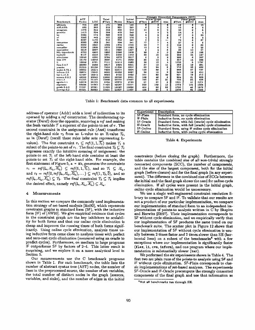
Our measurements use the C benchmark programs shown in Table 1. For each benchmark, the table lists the number of abstract syntax tree (AST) nodes, the number of lines in the preprocessed source, the number of set variables, the total number of distinct nodes in the graph (sources, variables, and sinks), and the number of edges in the initial

Experiment 1 Description SF-Plain I Standard form. no cycle elimination IF-Plain Inductive form; no c&zle elimination SF-Oracle Standard form, with full (oracle) cycle elimination IF-Oracle Inductive form, with full (oracle) cycle elimination SF-Online Standard from, using IF online cycle elimination IF-Online Inductive form, with online cycle elimiuation

Table 4: Experiments

constraints (before closing the graph). Furthermore, the table contains the combined size of all non-trivial strongly connected components (SCC), the number of components, and the size of the largest component, both for the initial graph (before closure) and for the final graph (in any experiment). The difference in the combined size of SCCs between the initial and the final graph shows the need for online cycle elimination. If all cycles were present in the initial graph, online cycle elimination would be unnecessary.

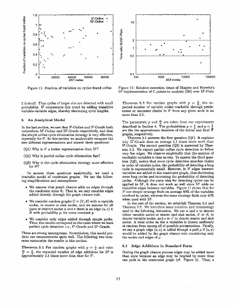
We use a single well-engineered constraint resolution li- brary to compare SF and IF. To validate that our results are not a product of our particular implementation, we compare our implementation of standard form to an independent implementation of points-to analysis written in C by Shapiro and Horwitz [SH97]. Their implementation corresponds to SF without cycle elimination, and we empirically verify that our implementation of SF produces the same trend on our benchmark suite. The scatter plot in Figure 12 shows that our implementation of SF without cycle elimination is usually between 2 times faster and 2 times slower than SH (hor- izontal lines) on a subset of the benchmarks4 with a few exceptions where our implementation is significantly faster (flex, li, cvs, inform), and one program where our implementation is substantially slower (tar).

We performed the six experiments shown in Table 4. The first two are plain runs of the points-to analysis using SF and IF without cycle elimination. SF-Plain corresponds to clas- sic implementations of set-based analyses. The experiments SF-Oracle and IF-Oracle precompute the strongly connected components of the final graph and use that information as

‘Not all benchmarks ran through SH.

90

Be”.hnlMk Edges allroots 384 diff.diffh ,11 Dnngrnm 610 genetic 515 ks 3386 “1 315 ft 3766 co”lpr+o* 402 rcMor 5777 compiler 2733 c.ssembler 5219 ML-typecheek 17908 eqntott 15667 sinwlntor 29935 l~S*-l?? 76789 li 113042, flex-2.4.7 98301 pmake 364732 mnke-3.72.1 74,878 inform-5.5 236017 tnr-1.11.2 278820 screen-3.6.2 963242 EVB-1 .a 214220 agmls-1.1 1706442 e*premo 859093 gawk-3.0.3 1653812 povmy-2.2 2710342

IF-Ph,rl Work

441 782 557 672

15362 428

19821 742

24887 3648 9844

169253 132260 6718.36

3047616 177872021

2231538 28462390 Q6349223 1623679.5 181?5919

130Pi98316 6702128

362820558 78018098

267208OQ3 490070572

Time(s)

008 0:13 0.09 0.13 0.46 0.11 0.61 0.15 1.30 0.61 1.21 5.38 3.63

14.48 64.43

4349.04 62.20

669.97 2287.20

359.31 433.98

2988.00 161.33

8686.46 1903.74 6605.69

12159.00

Edges aQo

606 412 446

1278 280

1204 366

3168 3027 4016

21860 4291

36280 72045

1740142 15736

306771 6Q3860 222182 250474 640161 116513

14,264, 741816 922422

1084147

300 661 450 406

2332 381

1733 520

5070 3992 4916

14Q501 ,085

28285, 678170

10363Q138 27498

8582058 43941107

.5606608 5842830

3879,130 8Q1083

140867874 23276456 414QQ85,

179010002

Time(s) 0.06

0.11 0.10 0.10 0.17 0.10 0.10 0.14 0.60 0.50 0.85 3.45 0.86 8.07

12.51 1629.02

4.70 134.45 624.01

90.64 80.30

610.8, 22.96

2077.24 373.30 686.Q2

2966.48

Edges

322 686 450 488 663 301

1008 376

2302 2.571 3552 3826 2927 4838 8412

13360 12954 15485 10967 31091 18711

- 26364 26050 32318

-

Work 907

762 483 542 078 414

1251 570

3309 3378 4326 GOOK 4030 6578

13796 76391 20795 4,806

119389 OS132 37260

-

43685 179301 123335

-

s

Time(s) ---Km

0.10 0.07 0.10 0.15 0.13 0.33 0.13 0.62 0.72 1.44 1.24 1.06 1.Q8 3.31

10.62 6.61 6.00

12.24 14.53

6.81 -

9.08 10.15 15.46

-

Table 2: Benchmark data for IF-Plain, SF-Plain, IF-Oracle, and SF-Oracle

Edges

261 688 369 432 850 272 832 317

2407 2655 3640 6606 2682

1296, 34029

470045 13100

133477 268863 11543,

84316 -

67253 532076 343268

jF-Olacl Work

284 OS? 393 481

1181 373

1024 403

3470 3476 4367 QJQ2 3868

16140 49028

786496 2114,

234533 484661 178675 136277

106422 905743 591302

-

AST

700 936

1078 1412 2284 2306 3027 3333 6269 5326 6316 0762 811,

10040 15119 16828 29960 31210 36892 38874 41407 49282 51223 53874 56038 71081 8,391

see #Vnrs

10 13 23 14 37

7 'IO 2,

104 a9 06

206 232 290 357

1736 356 775 866 606 831 804 75.5

1201 1773 17913 1678

n- Elim. Edges 10 -xc

7 697 IS 493

6 602 31 1136

4 308 44 1390 15 448 64 2893 17 2703 70 4061

238 6519 163 4074 206 ,344 269 10943

1284 28386 279 14678 660 21413 786 40498 422 35374 674 24216 781 39728 581 30677

1075 46568 1231 41390 1438 36103 1292 8,130

Work The(*) 408 o.00

767 0.11 536 0.11 556 0.13

1742 0.23 419 0.11

1800 0.29 669 0.16

4168 0.0, 3524 0.72 5016 1.13

11168 1.67 6264 1.10

14366 2.89 18121 3.65

1669.51 30.25 23842 6.50 83686 14.94

283025 40.10 110442 18.64

50122 0.20 235411 40.6,

52408 12.91 314633 63.55 155881 27.89 176OQ7 31.16 336573 58.63

Elim. 7

: 2

13 1

22 10 15

6 26 40 56 Ql

141 678 12.5 291 479 260 413 553 263 830 515 615 782

Edges 286

607 407 444

1182 270

1241 356

3079 3013 4004

21158 SD31

32521 58106

1260930 15246

213492 471810 168QTQ 153672 384080

89744 901331 54.5501 SQOBSQ

1382071

Table 3: Benchmark data for IF-Online and SF-Online

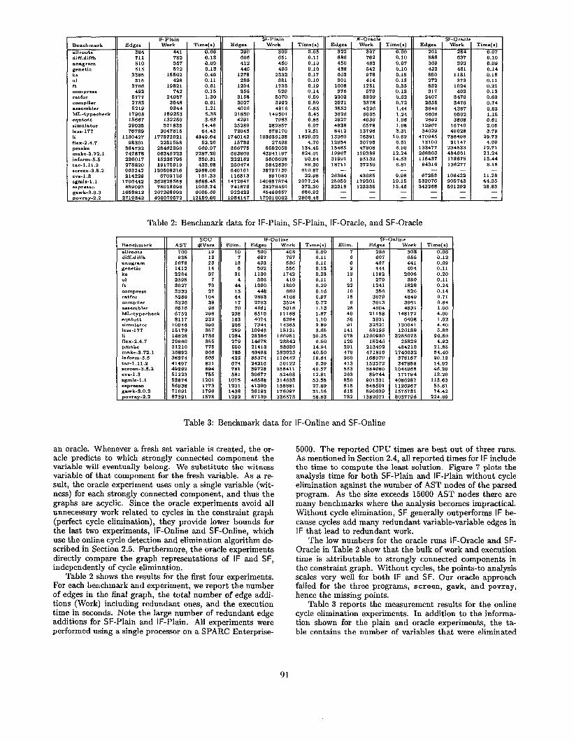
an oracle. Whenever a fresh set variable is created, the oracle predicts to which strongly connected component the variable will eventually belong. We substitute the witness variable of that component for the fresh variable. As a result, the oracle experiment uses only a single variable (witness) for each strongly connected component, and thus the graphs are acyclic. Since the oracle experiments avoid all unnecessary work related to cycles in the constraint graph (perfect cycle elimination), they provide lower bounds for the last two experiments, IF-Online and SF-Online, which use the online cycle detection and elimination algorithm described in Section 2.5. Furthermore, the oracle experiments directly compare the graph representations of IF and SF, independently of cycle elimination.

Table 2 shows the results for the first four experiments. For each benchmark and experiment, we report the number of edges in the final graph, the total number of edge additions (Work) including redundant ones, and the execution time in seconds. Note the large number of redundant edge additions for SF-Plain and IF-Plain. All experiments were performed using a single processor on a SPARC Enterprise-

Work TitlW(*)

305 0.08 656 0.12 441 0.00 494 0.11

2006 0.20 380 0.11

1828 0.24 526 0.14

4849 0.71 3961 0.64 4831 1.00

148172 4.00 0408 1.02

130041 4.40 126138 6.83

3285073 06.88 25828 4.92

484218 21.86 1740032 54.40

3,815, 20.13 347858 14.92

1044965 46.29 1,1,94 13.20

4086267 113.63 1126267 55.61 ll?b?31 74.42 8037706 224.80

Time(n) 0.07

0.10 0.09 0.14 0.15 0.11 0.21 0.13 0.63 0.74 0.83 1.15 0.81 2.05 3.79

29.73 4.99

12.71 21.24 13.44

8.15 -

11.28 44.35 28.83

-

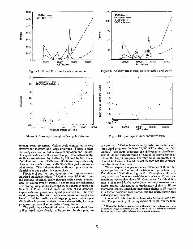
5000. The reported CPU times are best out of three runs. As mentioned in Section 2.4, all reported times for IF include the time to compute the least solution. Figure 7 plots the analysis time for both SF-Plain and IF-Plain without cycle elimination against the number of AST nodes of the parsed program. As the size exceeds 15000 AST nodes there are many benchmarks where the analysis becomes impractical. Without cycle elimination, SF generally outperforms IF because cycles add many redundant variable-variable edges in IF that lead to redundant work.

The low numbers for the oracle runs IF-Oracle and SF- Oracle in Table 2 show that the bulk of work and execution time is attributable to strongly connected components in the constraint graph. Without cycles, the points-to analysis scales very well for both IF and SF. Our oracle approach failed for the three programs, screen, gawk, and povray, hence the missing points.

Table 3 reports the measurement results for the online cycle elimination experiments. In addition to the information shown for the plain and oracle experiments, the table contains the number of variables that were eliminated

91

6000 -

200

150

100

50

0 20000 40000 60000 8OOcxl

AST nodes 20000 40000 60000 80000

AST nodes

Figure 7: SF and IF without cycle elimination Figure 8: Analysis times with cycle detection and oracle

5

4.5 -

20 - *

++ 0; +

10 - xx +

++ + 5- r:

,

3.5 - .

3 -

2- $.. + +

+

1 - + i$ :g +:

0.5 ’ F ‘I .+., . ‘I . ’ ‘( ‘I . + 0.01 0.1 10 loo

Adolute time(s) SF-Plain 1000 10000

2.5 - . . 0

2 - .

1.5 - l * . o .

1 foe . l .

0.66 +- 2 __________-_ -- _____ 2 ___-_- _-_- _________-_-- - _-___ -_-.-- ------ _-_-

0 20000 40000 60000 80000 AST nodes

Figure 9: Speedups through online cycle detection Figure 10: Speedups through inductive form

through cycle detection. Online cycle elimination is very effective for medium and large programs. Figure 8 plots the analysis times for online cycle elimination and the oracle experiments (note the scale change). The fastest analysis times are achieved by IF-Oracle, followed by SF-Oracle, IF-Online, and then SF-Online. IF-Online stays relatively close to the oracle times, while SF-Online performs some- what worse. This indicates that while our cycle detection algorithm is not perfect, it comes close.

Figure 9 shows the total speedup of our approach over standard implementations (IF-Online over SF-Plain), and the speedup obtained solely through online cycle elimination (SF-Online over SF-Plain). To show that our techniques help scaling, we plot the speedups vs. the absolute execution time of SF-Plain. As the execution time of the standard implementation grows, our speedup also grows. For very small programs, the cost of cycle elimination outweighs the benefits, but for medium and large programs, online cycle elimination improves analysis times substantially, for large programs by more than an order of magnitude.

The performance benefit of inductive over standard form is illustrated more clearly in Figure 10. In this plot, we

250

can see that IF-Online is consistently faster for medium and large-sized programs (at least 10,000 AST nodes) than SF- Online.6 For large programs the difference is significant, with IF-Online outperforming SF-Online by over a factor of 3.8 for the largest program. For very small programs, IF is at most 50% slower than SF, which in absolute times means only fractions of seconds.

We can explain the performance difference of IF and SF by comparing the fraction of variables on cycles found by IF-Online and SF-Online (Figure 11). Throughout, SF finds only about half as many variables on cycles as IF, and the remaining cycles slow down SF. One reason for this difference is that for SF, the cycle detection only searches successor chains. The analog to predecessor chains in SF are increasing chains. Searching increasing chains in SF results in a higher detection rate (57%), but the much higher cost outweighs any benefits.

Our model in Section 5 explains why SF finds fewer cycles. The probability of finding chains of length greater than

‘The outlier is the program flex; although flex is a large program, it contains large iuitialised arrays. Thus as far as points-to analysis is concerned, it actually behaves like a small program.

92

1.2 IF-Online l

SF-Online + 1 l *

P 0 0

+

0.8 - * :, l * ** 4 * .

l * . . . . + o* 0 +

0.6 - +* ++ * .I +

+ + +

OL 0 20000 40000 60000 80000

AST nodes

Figure 11: Fraction of variables on cycles found online

2 is small. Thus cycles of larger size are detected with small probability. IF counteracts this trend by adding transitive variable-variable edges, thereby shortening cycle lengths.

5 An Analytical Model

In the last section, we saw that IF-Online and IF-Oracle both outperform SF-Online and SF-Oracle respectively, and that the simple online cycle elimination strategy is very effective, especially for IF. In this section we analytically compare the two different representations and answer three questions:

(Ql) Why is IF a better representation than SF?

(Q2) Why is partial online cycle elimination fast?

(Q3) Why is the cycle elimination strategy more effective for IF?

To answer these questions analytically, we need a tractable model of constraint graphs. We use the following simplifications and assumptions:

l We assume that graph closure adds no edges through the resolution rules R. That is, we only consider edges added directly through the graph closure rule.

. We consider random graphs G = (V, E) with n variable nodes, m source or sink nodes, and we assume for all pairs of distinct nodes u and v there is an edge (u, v) E E with probability p, for some constant p.

l We consider only edges added through simple paths. Thus, the results correspond to the cases where we have perfect cycle detection i.e., IF-Oracle and SF-Oracle.

These are strong assumptions. Nevertheless, this model predicts our measurements quite well. The following two theo- rems summarize the results in this section.

Theorem 5.1 For random graphs with p = $ and ratio L?l=z the expected number of edge additions for SF is approx!mately 2.5 times more than that for IF.

10

2

1

0.5

0.1 100 1000 10000 100000

AST nodes

Figure 12: Relative execution times of Shapiro and Horwitz’s SF implementation of C points-to analysis (SH) over SF-Plain

Theorem 5.2 For random graphs with p = f, the expected number of variable nodes reachable through predecessor or successor chains in IF from any given node is no more than 2.2.

The parameters p and f are taken from our experiments described in Section 4. The probabilities p = i and p = $ are the the approximate densities of the initial and final IF graphs, respectively.

Theorem 5.1 answers the first question (Ql). It explains why SF-Oracle does on average 4.1 times more work than IF-Oracle. The second question (Q2) is answered by Theo- rem 5.2. We expect partial online cycle detection to follow very few edges. We observe empirically that the number of reachable variables is close to two. To answer the third question (Q3), notice that since cycle detection searches chains in order of variable index, the probability of detecting a long cycle is exponentially small. However, in IF edges between variables are added to the constraint graph, thus shortening some long cycles and increasing the probability of detecting cycles. Although the same idea for detecting cycles can be applied to SF, it does not work as well since SF adds no transitive edges between variables. Figure 11 shows that for IF our simple strategy I?nds on average 80% of the variables involved in cycles, whereas the same strategy finds only 40% when used with SF.

In the rest of the section, we establish Theorem 5.1 and Theorem 5.2. We introduce some notation and terminology used in the following discussion. We use u and v to denote either variable nodes or source and sink nodes, X or Xi to denote variable nodes, and c or c’ to denote source and sink nodes. A total order on the n variables is chosen uniformly at random from among all n! possible permutations. Finally, we say a graph edge (u, v) is added through a path p if (u, v) would be added by the graph closure rule considering only the nodes and edges of p.

5.1 Edge Additions in Standard Form

During the graph closure process edges may be added more than once because an edge may be implied by more than one path in the constraint graph (cf. Figure 2). Thus, a

93

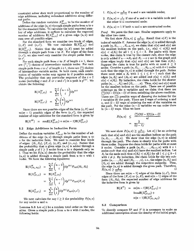
constraint solver does work proportional to the number of edge additions, including redundant additions along different paths.

Define the random variables XfL,V, to be the number of additions of the edge (u, v) through simple paths from u to v for the standard form. To calculate the total expected number of edge additions, it suffices to calculate the expected number of additions E(X&,) of a given edge (u,v) and sum over all possible edges.

For the standard form we consider two kinds of edges, (c, X) and (c,c’). We now calculate E(X&)) and

W&I ,I. Notice that the edge (c,X) must be added through a simple path from c to X. For edges of the form (c, c’), we also need only consider the simple paths from c to c’.

For each simple path from c to X of length i + 1, there are (“T1) choices of intermediate variable nodes. For each simpie’path from c to c’ of length i + 1, there are (y) choices of intermediate variable nodes. In both cases, each combi- nation of variable nodes may appear in i! possible orders. The probability that any particular sequence of the i + 2 nodes (including c and X or c and c’) is a path is p’+‘. We obtain the following:

W&)) = g p ; 1) i!pi+l i=l \ /

E(X&)) = 2 ; i!p”+’ 0 i=l \-/

Since there are mn. possible edges of the form (c, X) and m(m - 1) possible edges of the form (c,c’), the expected number of edge additions for the standard form is given by

E(X”) = mnE(X&)) + m(m - l)E(X&,))

5.2 Edge Additions in Inductive Form

Defme the random variables X&l to be the number of additions of the edge (u,v) through simple paths from u to v for the inductive form. We need to consider four kinds of edges: (Xr, Xe), (X,c), (c, X), and (cr,ce). Notice that the probability that a given edge (u,v) is added through a simple path p of 1 2 3 nodes from u to v depends only on 1. Thus we let Pi(u,v) denote the probability that the edge (u,v) is added through a simple path from u to v with i nodes. We have the following equations:

i!pif1Pi+2(Xly X2)

=

E(X[F,,=,l) = 2 ; i!pi+‘Pi+2(c,c’)

id 0

We next calculate for any 1 1 3 the probability PI (u, v) for any nodes u and v.

Lemma 5.3 Let o(.) be a random total order on the variables. Given a simple path p from u to v with 2 nodes, the following holds:

1. Pi (u, v) = I&J if u and v are variable nodes;

2. Pi(u, v) = & if one of u and v is a variable node and the other is a constructed node;

3. Pl (u, v) = 1 if both u and v are constructed nodes.

Proof. We prove the first case. Similar arguments apply to the other two cases.

We first show Pl(u,v) 5 &. Recall that o(X) is the index of variable X. Assume the edge (21, v) is added through apath (u,Xr,... , Xl-s,v), we claim that O(U) and o(v) are the smallest indices on the path, i.e., O(U) < o(Xi) and o(v) < o(Xi) for all 1 5 i 2 1 - 2. For paths with three nodes, this claim is true by the closure rule, since the edge is only added if u +...+Xl and Xi + v are in the graph and, these edges imply that o(u) and o(v) are less than o(Xr). Suppose the claim is true for paths with at most k 2 3 nodes. Consider a path (‘IL, Xl,. . . ,X,-r, v) with k+l nodes such that the edge (u, v) is added through the path. Notice there must exist a Xi with 1 5 i 5 k - 1 such that the edges (u, Xi) and (Xi,v) are added and O(U) < o(Xi) and o(v) < o(Xi). By induction, the claim holds for the shorter paths (u, . . . ,Xi)and(Xi,... , v). Thus, o(u) and o(v) must be the smallest indices on the path. There are n! possible orderings on the n variables and we claim that there are (7)(2(E - 2)!)(n - Z)! of th em satisfying the above condition. There are (1) possible ways of choosing the indices for the 1 variables on the path. There are 2 ways of ordering u and v, and (I - 2)! ways of ordering the rest of the variables on the path. For the other (n - 1) variables we can order them in (n - 1)! ways. Thus we have

fi(%V) 5 (;) (2(Z - 2)!)(n - I)!

I 71. 2

= l(l-l)’

We now show Pl(u,v) 2 &. Let o(e) be an ordering such that O(U) and o(v) are the smallest indices on the path &,X1,... , Xl,v). We show that the edge (u, v) is added through the path. The claim is clearly true for paths with three nodes. Suppose the claim holds for paths with at most k nodes. Consider a path (u, Xl,. . . , Xk-1, v) with k + 1 nodes such that O(U) and o(v) have the smallest indices. Let Xi be the node such that o(Xi) < o(Xj) for all 1 5 j 5 k - 1 with i # j. By induction, the claim holds for the two subpaths (u, . . . ,Xi) and(Xi,... , v), i.e., the edges (u, Xi) and (Xi,v) are added through the respective subpaths. Thus, the edge (u, v) is added through the given path. Therefore, fi(u,v) 2 q&j. 0

Since there are m(m - 1) edges of the form (c,c’), 2mn edges of the form (X, c) or (c, X), and n(n - 1) edges of the form (Xl, X2), the expected number of edge additions for the inductive form is given by

E(XIF) = m(m - l)E(X[:,c~l) +

2mnE(X$,d +

n(n - ~)W%,X~))

5.3 Comparison

To directly compare SF and IF it is necessary to make an additional assumption about the density of the initial graph.

94

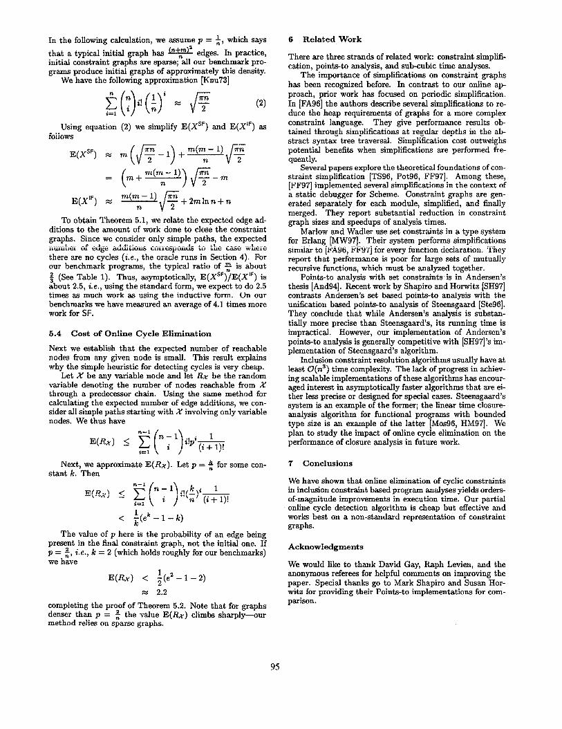
In the following calculation, we assume p = $, which says

that a typical initial graph has @$ edges. In practice, initial constraint graphs are sparse; all our benchmark programs produce initial graphs of approximately this density.

We have the following approximation [Knu73]

(2)

Using equation (2) we simplify E(XsF) and E(XIF) as follows

E(X”) x m(E-1) -l-mcm~l)~

To obtain Theorem 5.1, we relate the expected edge additions to the amount of work done to close the constraint graphs. Since we consider only simple paths, the expected number of edge additions corresponds to the case where there are no cycles (i.e., the oracle runs in Section 4). For our benchmark programs, the typical ratio of z is about $ (See Table 1). Thus, asymptotically, E(XsF)/E(XIF) is about 2.5, i.e., using the standard form, we expect to do 2.5 times as much work as using the inductive form. On our benchmarks we have measured an average of 4.1 times more work for SF.

5.4 Cost of Online Cycle Elimination

Next we establish that the expected number of reachable nodes from any given node is small. This result explains why the simple heuristic for detecting cycles is very cheap.

Let X be any variable node and let RX be the random variable denoting the number of nodes reachable from X through a predecessor chain. Using the same method for calculating the expected number of edge additions, we consider all simple paths starting with X involving only variable nodes. We thus have

Next, we approximate E(Rx). Let p = $ for some constant k. Then

< ;(ek-l-k)

The value of p here is the probability of an edge being present in the final constraint graph, not the initial one. If P= $, i.e., k = 2 (which holds roughly for our benchmarks) we have

E(Rx) < ;(e2-1 -2)

x 2.2

completing the proof of Theorem 5.2. Note that for graphs denser than p = 2 the value E(Rx) method relies on s;arse graphs.

climbs sharply-our

6 Related Work

There are three strands of related work: constraint simplification, points-to analysis, and sub-cubic time analyses.

The importance of simplifications on constraint graphs has been recognized before. In contrast to our online approach, prior work has focused on periodic simplification. In [FA96] the authors describe several simplifications to reduce the heap requirements of graphs for a more complex constraint language. They give performance results obtained through simplifications at regular depths in the abstract syntax tree traversal. Simplification cost outweighs potential benefits when simplifications are performed fre- quently.

Several papers explore the theoretical foundations of constraint simplification [TS96, Pot96, FF97]. Among these, [FF97] implemented several simplifications in the context of a static debugger for Scheme. Constraint graphs are generated separately for each module, simplified, and finally merged. They report substantial reduction in constraint graph sizes and speedups of analysis times.

Marlow and Wadler use set constraints in a type system for Erlang [MW97]. Their system performs simplifications similar to [FA96, FF97] for every function declaration. They report that performance is poor for large sets of mutually recursive functions, which must be analyzed together.

Points-to analysis with set constraints,is in Andersen’s thesis [And94]. Recent work by Shapiro and Horwitz [SH97] contrasts Andersen’s set based points-to analysis with the unification based points-to analysis of Steensgaard [SteSG]. They conclude that while Andersen’s analysis is substantially more precise than Steensgaard’s, its running time is impractical. However, our implementation of Andersen’s points-to analysis is generally competitive with [SH97]‘s implementation of Steensgaard’s algorithm.

Inclusion constraint resolution algorithms usually have at least O(n3) time complexity. The lack of progress in achiev- ing scalable implementations of these algorithms has encour- aged interest in asymptotically faster algorithms that are either less precise or designed for special cases. Steensgaard’s system is an example of the former; the linear time closure- analysis algorithm for functional programs with bounded type size is an example of the latter [Mos96, HM97]. We plan to study the impact of online cycle elimination on the performance of closure analysis in future work.

7 Conclusions

We have shown that online elimination of cyclic constraints in inclusion constraint based program analyses yields orders- of-magnitude improvements in execution time. Our partial online cycle detection algorithm is cheap but effective and works best on a non-standard representation of constraint graphs.

Acknowledgments

We would like to thank David Gay, Raph Levien, and the anonymous referees for helpful comments on improving the paper. Special thanks go to Mark Shapiro and Susan Hor- witz for providing their Points-to implementations for comparison.

95

References

[And941

[AW92]

[AW93]

[AWL941

[FA96]

[FFS’I]

[FFA97]

L. 0. Andersen. Program Analysis and Special- ization for the C Progmmmkzg Language. PhD thesis, DIKU, University of Copenhagen, May 1994. DIKU report 94/19.

A. Aiken and E. Wimmers. Solving Systems of Set Constraints. In Symposium on Logic in Com- puter Science, pages 329-340, June 1992.

A. Aiken and E. Wimmers. Type Inclusion Con- straints and Type Inference. In Proceedings of the 1993 Conference on Functional Programming Languages and Computer Architecture, pages 31- 41, Copenhagen, Denmark, June 1993.

A. Aiken, E. Wimmers, and T.K. Lakshman. Soft typing with conditional types. In Twenty-First Annual ACM Symposium on Principles of Pro- gramming Languages, January 1994.

M. Ftindrich and A. Aiken. Making Set- Constraint Based Program Analyses Scale. In First Workshop on Set Constraints at CP’g6, Cambridge, MA, August 1996. Available as Technical Report CSD-TR-96-917, University of California at Berkeley.

C. Flanagan and M. Felleisen. Componential Set- Based Analysis. In PLDI’97 [PLD97].

J. Foster, M. Ftindrich, and A. Aiken. Flow- Insensitive Points-to Analysis with Term and Set Constraints. Technical Report UCB//CSD-97- 964, U. of California, Berkeley, August 1997.

[FFK+96] C. Flanagan, M. Flat& S. Krishnamurthi, S. Weirich. and M. Felleisen. Catching Bugs in the Web of Program Invariants. In Pioceekgs of the 1996 ACM SIGPLAN Conference on Pro- gramming Language Design and Implementation, pages 23-32, May 1996.

[GJS96]

[Hei92]

[Hei94]

[HJ90]

[HM97]

[JM79]

James Gosling, Bill Joy, and Guy Steele. The Java Language Spec$cation, chapter 10, pages 199-200. Addison Wesley, 1996.

N. Heintze. Set Based Program Analysis. PhD thesis, Carnegie Mellon University, 1992.

N. Heintze. Set Based Analysis of ML Programs. In Proceedings of the 1994 ACM Conference on LISP and FPrnctional Programming, pages 306- 17, June 1994.

N. Heintae and J. Jaffar. A decision procedure for a class of Herbrand set constraints. In Sympo- sium on Logic in Computer Science, pages 42-51, June 1990.

N. Heintze and D. McAllester. Linear-Time Sub- transitive Control Flow Analysis. In PLDI’97 [PLD97].

N. D. Jones and S. S. Muchnick. Flow Anal- ysis and Optimization of LISP-like Structures. In Sk&h Annual ACM Symposium on Principles of Programming Languages, pages 244-256, Jan- uary 1979.

[Knu73]

[Koz93]

[MosSG]

[MTHSO]

[MW97]

[PLD97]

[Pot961

[PS91]

@w691

[SH97]

[ShiSS]

[Shm83]

[Ste96]

[TSSG]

D. Knuth. The Art of Computer Programming, Fundamental Algorithms, volume 1. Addison- Wesley, Reading, Mass., 2 edition, 1973.

D. Kozen. Logical Aspects of Set Constraints. In E. Bijrger, Y. Gurevich, and K. Meinke, editors, Proc. 1993 Conf. Computer Science Logic (CSL ‘93), volume 832 of Lecture Notes in Computer Science, pages 175-188. Springer-Verlag, 1993.

C. Mossin. Flow Analysis of Typed Higher-Order Programs. PhD thesis, DIKU, Department of Computer Science, University of Copenhagen, 1996.

Robin Milner, Mads Tofte, and Robert Harper. The Definition of Standard ML. MIT Press, 1990.

S. Marlow and P. Wadler. A Practical Subtyping System For Erlang. In Proceedings of the Inter- national Conference on Functional Programming (ICFP ‘97), June 1997.

Proceedings of the 1997 ACM SIGPLAN Confer- ence on Programming Language Design and Im- plementation, June 1997.

F. Pottier. Simplifying Subtyping Constraints. In Proceedings of the 1996 ACM SIGPLAN Inter- national Conference on Functional Programming (ICFP ‘961, pages 122-133, January 1996.

J. Palsberg and M. I. Schwartzbach. Object- Oriented Type Inference. In Proceedings of the ACM Conference on Object-Oriented programming: Systems, Languages, and Applications, October 1991.

J. C. Reynolds. Automatic Computation of Data Set Definitions, pages 456-461. Information Pro- cessing 68. North-Holland, 1969.

M. Shapiro and S. Horwitz. Fast and ACCU- rate Flow-Insensitive Points-To Analysis. In Pro- ceedings of the 84th Annual ACM SIGPLAN- SIGACT Symposium on Principles of Program- ming Languages, pages 1-14, January 1997.

0. Shivers. Control Flow Analysis in Scheme. In Proceedings of the ACM SIGPLAN ‘88 Confer- ence on Programming Language Design and Im- plementation, pages 164-174, June 1988.

0. Shmueli. Dynamic Cycle Detection. Informa- tion Processing Letters, 17(4):185-188, 8 Novem- ber 1983.

B. Steensgaard. Points-to Analysis in Almost Linear Time. In Proceedings of the i&d Annual ACM SIGPLAN-SIGACT Symposium on Ptin- ciples of Programming Languages, pages 32-41, January 1996.

V. Trifonov and S. Smith. Subtyping Con- strained Types. In Proceedings of the 3rd Inter- national Static Analysis Symposium, pages 349- 365, September 1996.

96

Documents

Partial Online Cycle Elimination in Inclusion Constraint Graphs