Embed Size (px)
Citation preview
PARTIAL DERIVATIVESPARTIAL DERIVATIVES
14
PARTIAL DERIVATIVES
14.6Directional Derivatives
and the Gradient Vector
In this section, we will learn how to find:
The rate of changes of a function of
two or more variables in any direction.
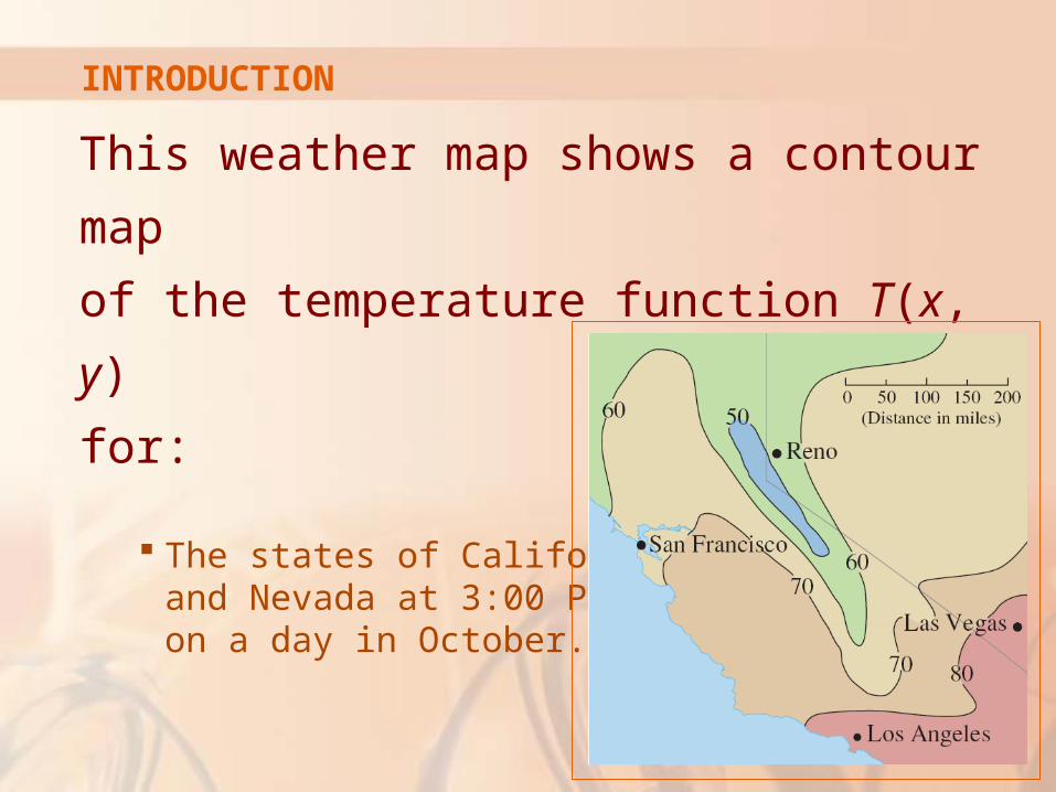
INTRODUCTION
This weather map shows a contour map
of the temperature function T(x, y)
for:
The states of California and Nevada at 3:00 PM on a day in October.
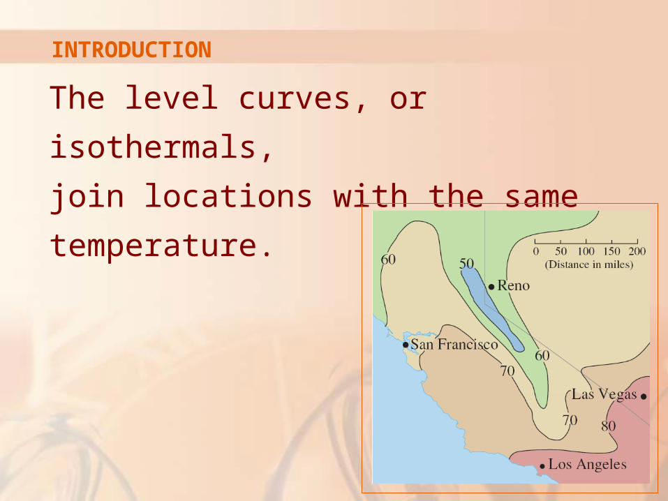
INTRODUCTION
The level curves, or isothermals,
join locations with the same
temperature.
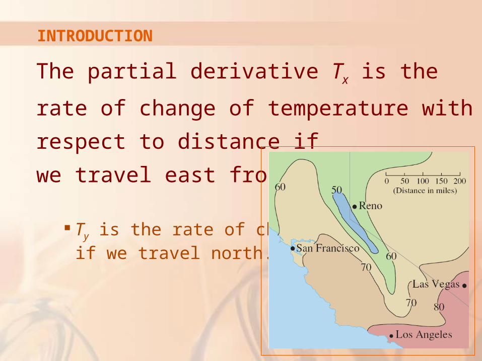
The partial derivative Tx is the rate of change
of temperature with respect to distance if
we travel east from Reno.
Ty is the rate of change if we travel north.
INTRODUCTION
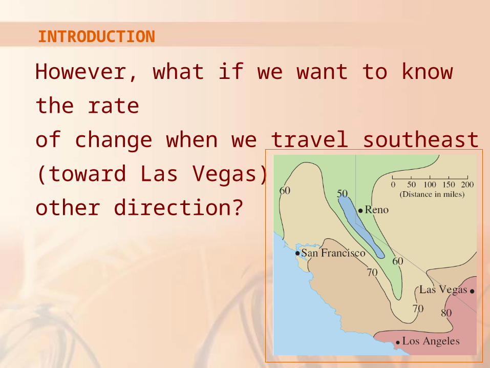
However, what if we want to know the rate
of change when we travel southeast (toward
Las Vegas), or in some other direction?
INTRODUCTION
In this section, we introduce a type of
derivative, called a directional derivative,
that enables us to find:
The rate of change of a function of two or more variables in any direction.
DIRECTIONAL DERIVATIVE
DIRECTIONAL DERIVATIVES
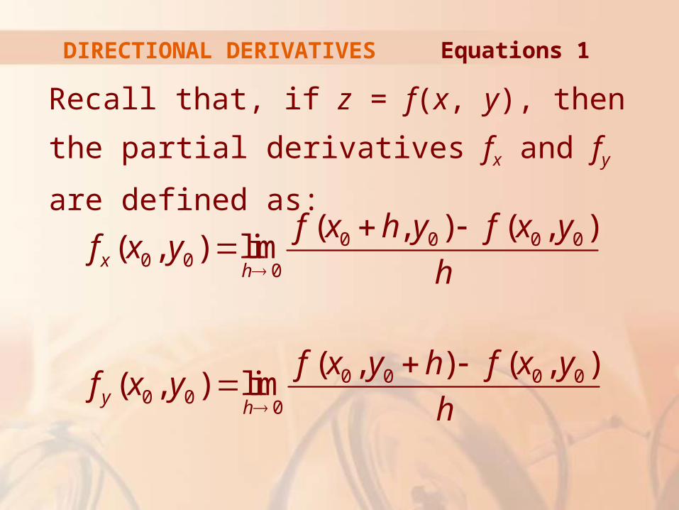
Recall that, if z = f(x, y), then the partial
derivatives fx and fy are defined as:
0 0 0 00 0
0
0 0 0 00 0
0
( , ) ( , )( , ) lim
( , ) ( , )( , ) lim
xh
yh
f x h y f x yf x y
h
f x y h f x yf x y
h
Equations 1
DIRECTIONAL DERIVATIVES
They represent the rates of change of z
in the x- and y-directions—that is, in
the directions of the unit vectors i and j.
Equations 1
DIRECTIONAL DERIVATIVES
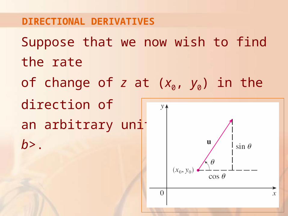
Suppose that we now wish to find the rate
of change of z at (x0, y0) in the direction of
an arbitrary unit vector u = <a, b>.
DIRECTIONAL DERIVATIVES
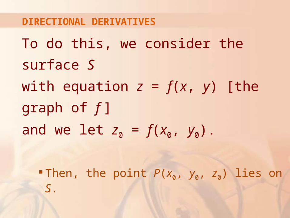
To do this, we consider the surface S
with equation z = f(x, y) [the graph of f ]
and we let z0 = f(x0, y0).
Then, the point P(x0, y0, z0) lies on S.
DIRECTIONAL DERIVATIVES
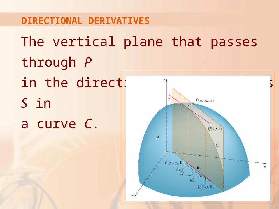
The vertical plane that passes through P
in the direction of u intersects S in
a curve C.
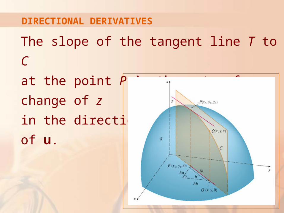
DIRECTIONAL DERIVATIVES
The slope of the tangent line T to C
at the point P is the rate of change of z
in the direction
of u.
DIRECTIONAL DERIVATIVES
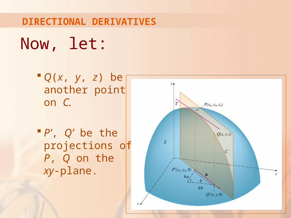
Now, let:
Q(x, y, z) be another point on C.
P’, Q’ be the projections of P, Q on the xy-plane.
DIRECTIONAL DERIVATIVES
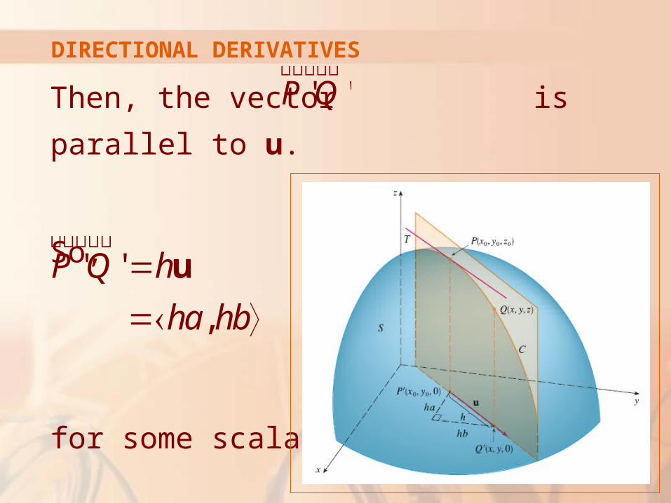
Then, the vector is parallel to u.
So,
for some scalar h.
' '��������������P Q
' '
,
P Q h
ha hb
u
��������������
DIRECTIONAL DERIVATIVES
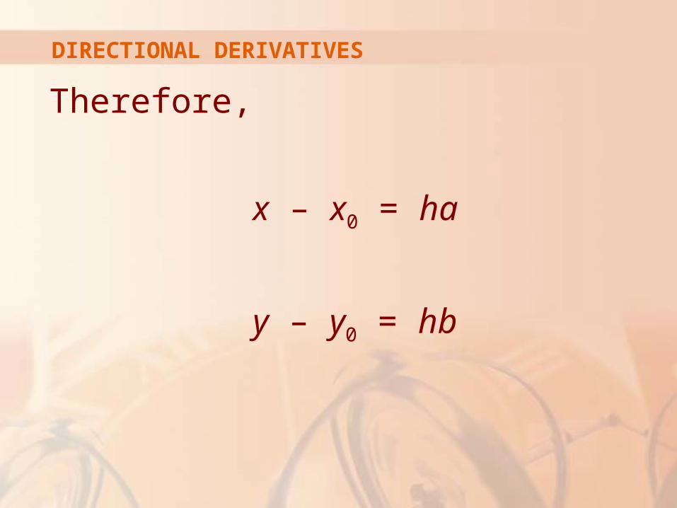
Therefore,
x – x0 = ha
y – y0 = hb
DIRECTIONAL DERIVATIVES
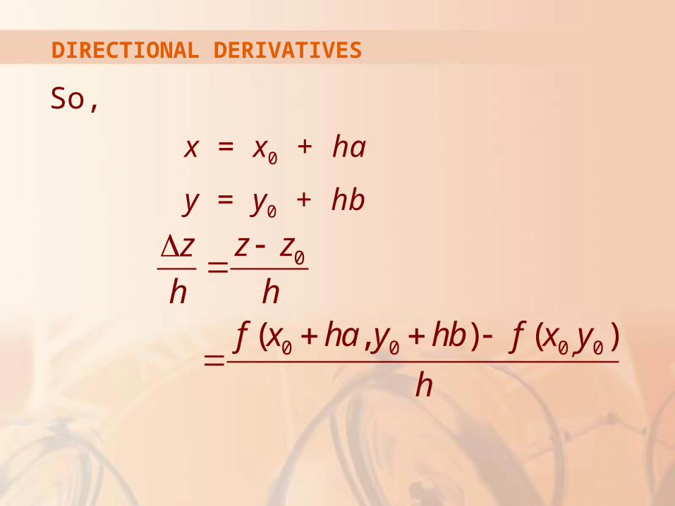
So,
x = x0 + ha
y = y0 + hb
0
0 0 0, 0( , ) ( )
z zz
h hf x ha y hb f x y
h
DIRECTIONAL DERIVATIVE
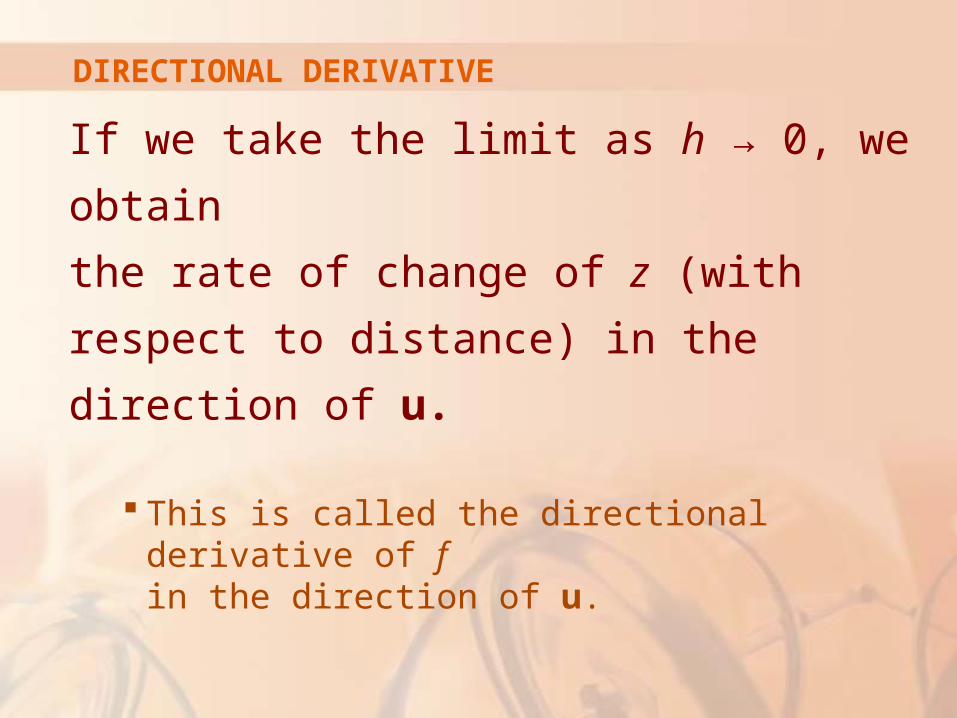
If we take the limit as h → 0, we obtain
the rate of change of z (with respect to
distance) in the direction of u.
This is called the directional derivative of f in the direction of u.
DIRECTIONAL DERIVATIVE
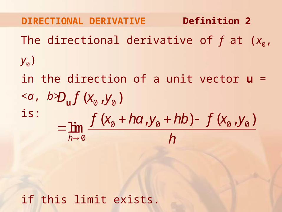
The directional derivative of f at (x0, y0)
in the direction of a unit vector u = <a, b>
is:
if this limit exists.
Definition 2
0 0
0 0 0 0
0
( , )
( , ) ( , )limh
D f x y
f x ha y hb f x y
h
u
DIRECTIONAL DERIVATIVES
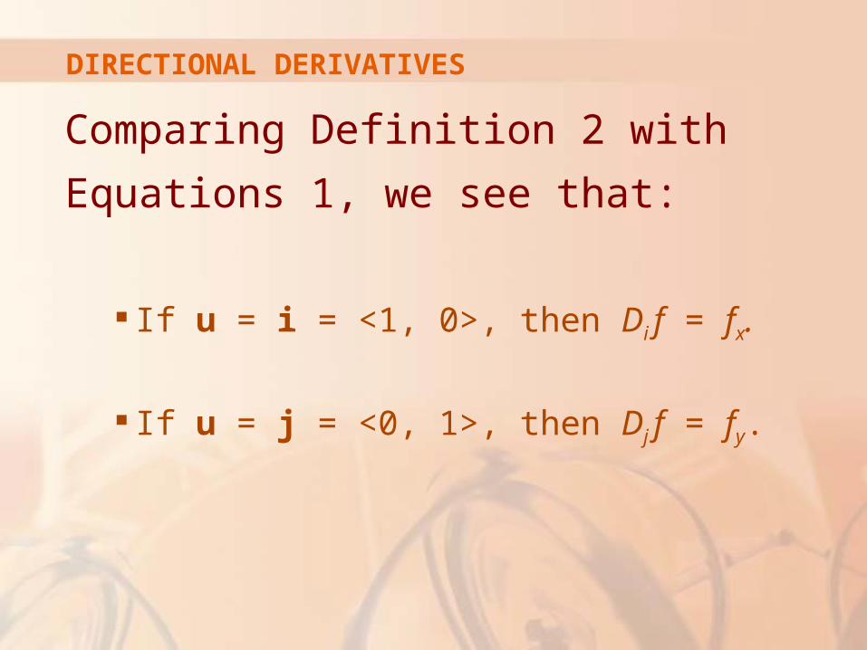
Comparing Definition 2 with Equations 1,
we see that:
If u = i = <1, 0>, then Di f = fx.
If u = j = <0, 1>, then Dj f = fy.
DIRECTIONAL DERIVATIVES
In other words, the partial derivatives of f
with respect to x and y are just special
cases of the directional derivative.
DIRECTIONAL DERIVATIVES
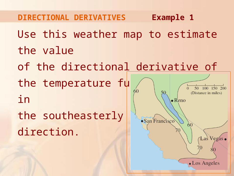
Use this weather map to estimate the value
of the directional derivative of the temperature
function at Reno in
the southeasterly
direction.
Example 1
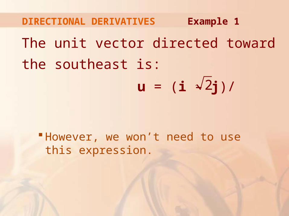
DIRECTIONAL DERIVATIVES
The unit vector directed toward
the southeast is:
u = (i – j)/
However, we won’t need to use this expression.
Example 1
2
DIRECTIONAL DERIVATIVES
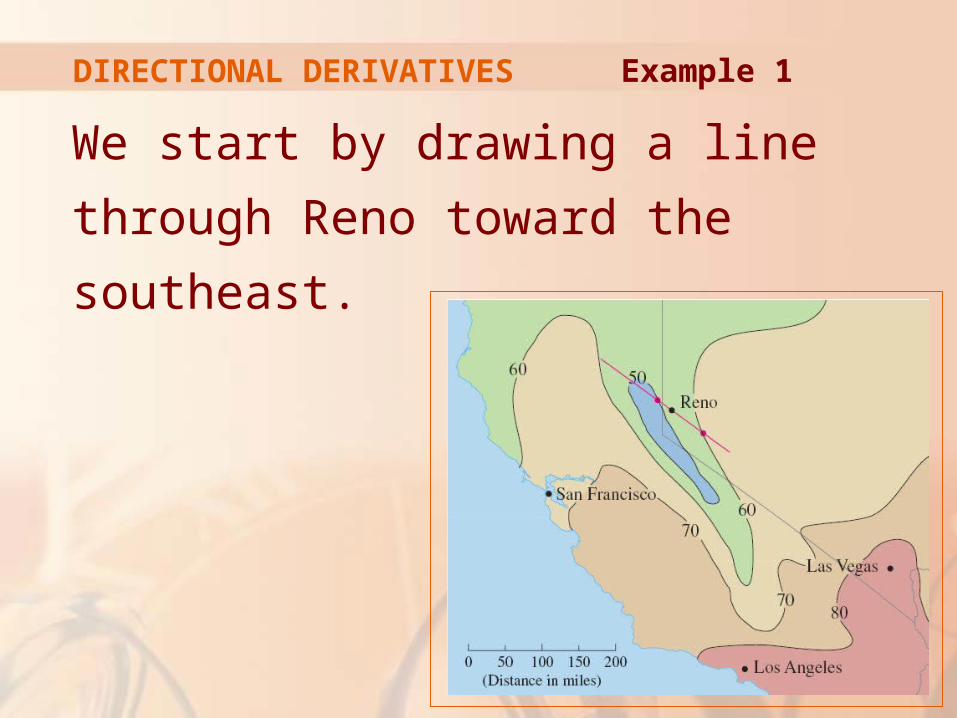
We start by drawing a line through Reno
toward the southeast.
Example 1
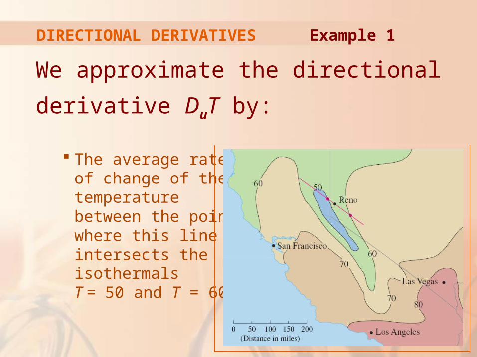
DIRECTIONAL DERIVATIVES
We approximate the directional derivative
DuT by:
The average rate of change of the temperature between the points where this line intersects the isothermals T = 50 and T = 60.
Example 1
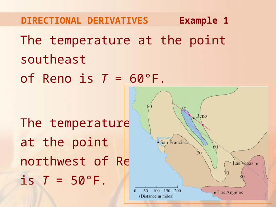
DIRECTIONAL DERIVATIVES
The temperature at the point southeast
of Reno is T = 60°F.
The temperature
at the point
northwest of Reno
is T = 50°F.
Example 1
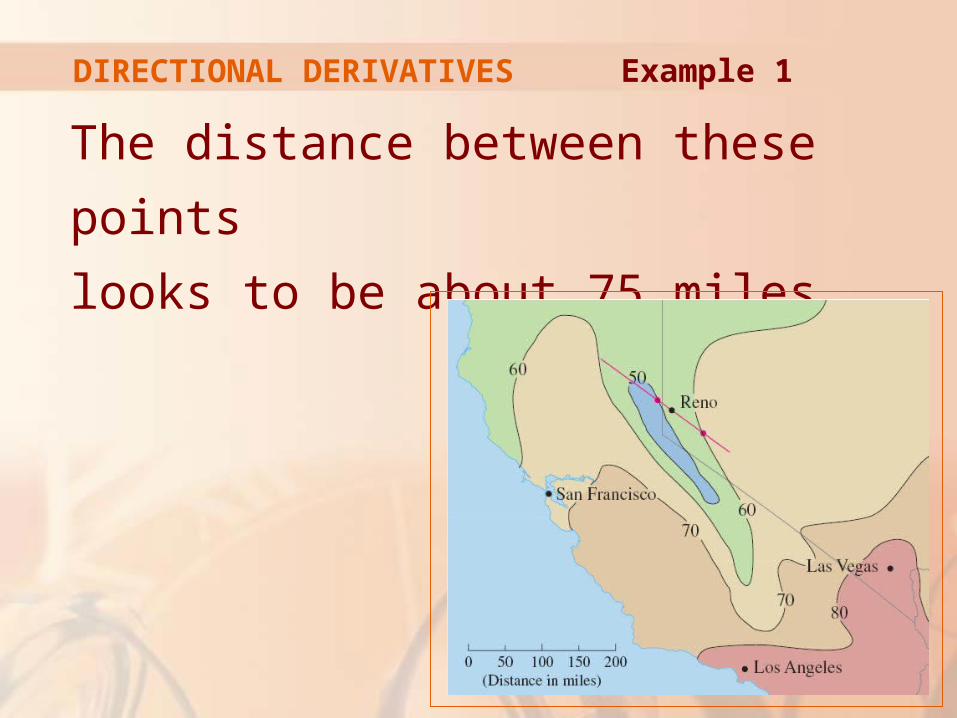
DIRECTIONAL DERIVATIVES
The distance between these points
looks to be about 75 miles.
Example 1
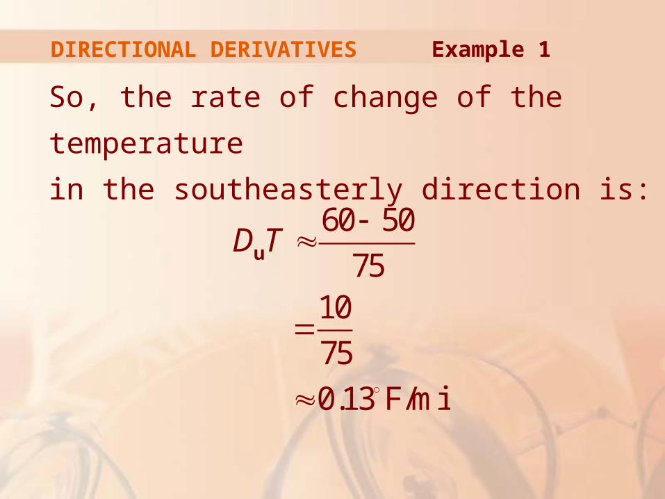
DIRECTIONAL DERIVATIVES
So, the rate of change of the temperature
in the southeasterly direction is:
Example 1
60 50
7510
75
0.13 F/mi
D T
u
DIRECTIONAL DERIVATIVES
When we compute the directional
derivative of a function defined by
a formula, we generally use the following
theorem.
DIRECTIONAL DERIVATIVES
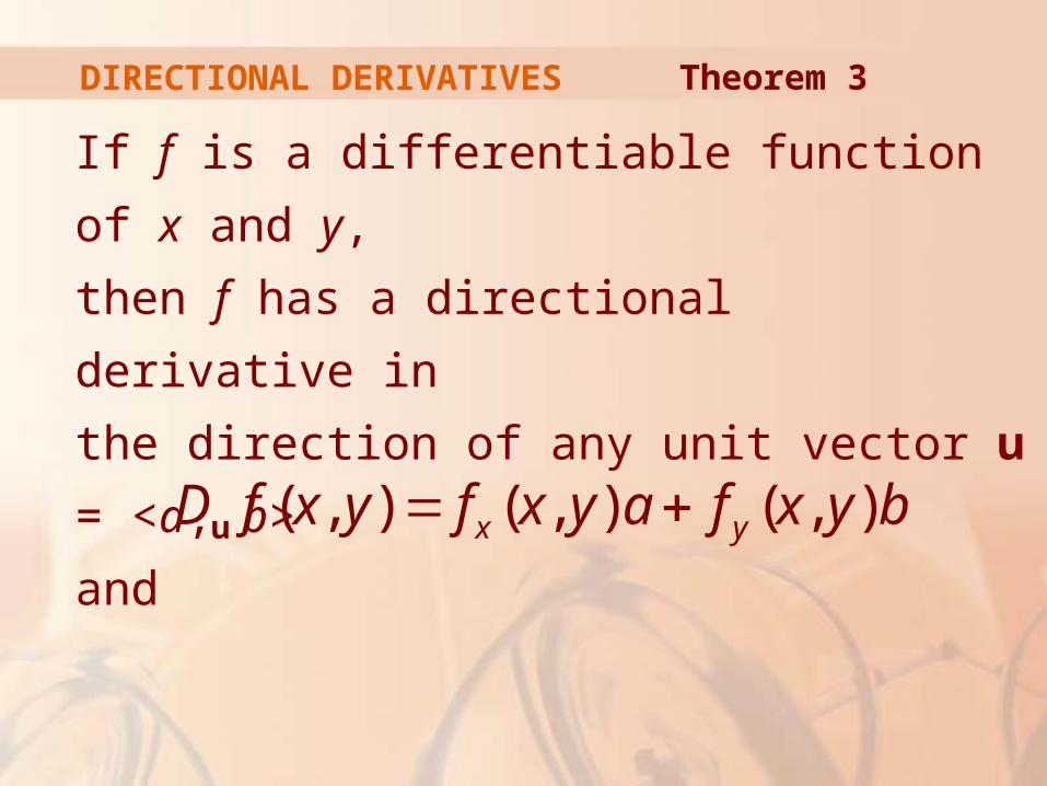
If f is a differentiable function of x and y,
then f has a directional derivative in
the direction of any unit vector u = <a, b>
and
Theorem 3
( , ) ( , ) ( , )x yD f x y f x y a f x y b u
DIRECTIONAL DERIVATIVES
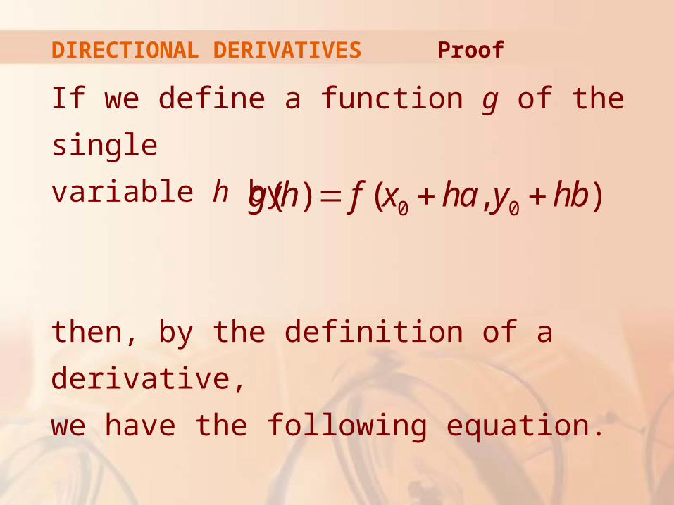
If we define a function g of the single
variable h by
then, by the definition of a derivative,
we have the following equation.
Proof
0 0( ) ( , ) g h f x ha y hb
DIRECTIONAL DERIVATIVES
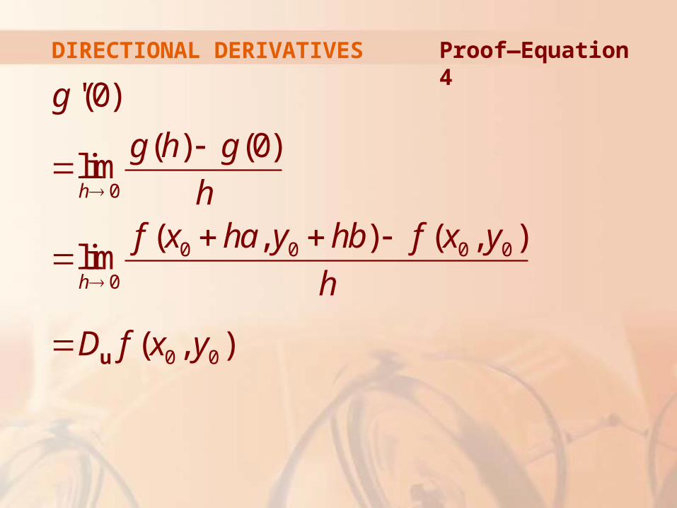
Proof—Equation 4
0
0 0 0 0
0
0 0
'(0)
( ) (0)lim
( , ) ( , )lim
( , )
h
h
g
g h g
hf x ha y hb f x y
h
D f x y
u
DIRECTIONAL DERIVATIVES
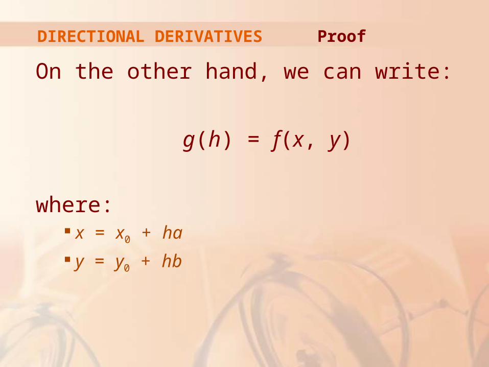
On the other hand, we can write:
g(h) = f(x, y)
where: x = x0 + ha
y = y0 + hb
Proof
DIRECTIONAL DERIVATIVES
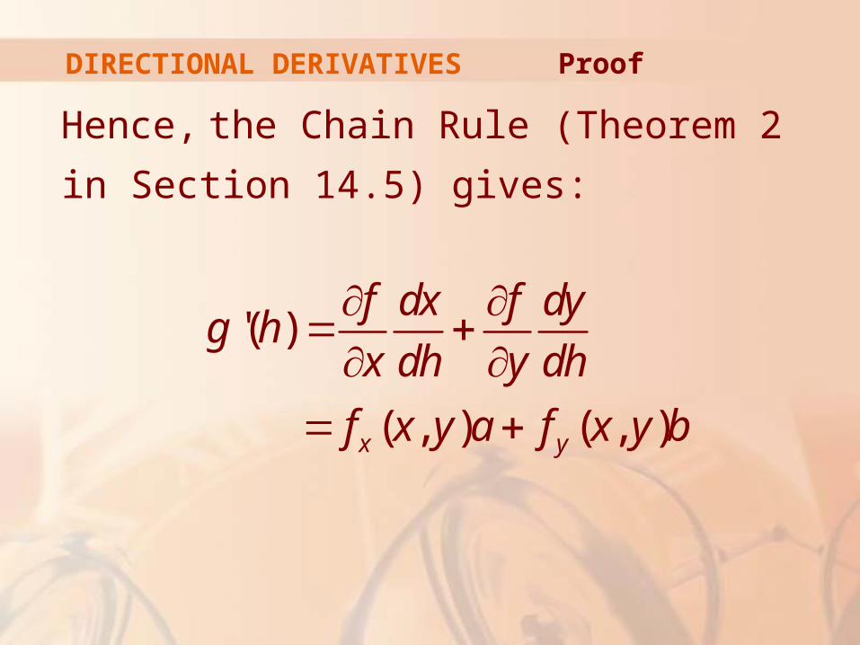
Hence, the Chain Rule (Theorem 2
in Section 14.5) gives:
'( )
( , ) ( , )x y
f dx f dyg h
x dh y dh
f x y a f x y b
Proof
DIRECTIONAL DERIVATIVES
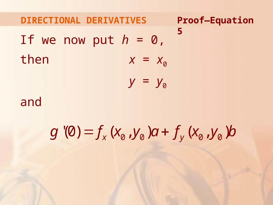
If we now put h = 0,
then x = x0
y = y0
and
0 0 0 0'(0) ( , ) ( , ) x yg f x y a f x y b
Proof—Equation 5
DIRECTIONAL DERIVATIVES
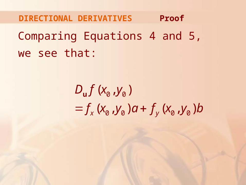
Comparing Equations 4 and 5,
we see that:
Proof
0 0
0 0 0 0
( , )
( , ) ( , )x y
D f x y
f x y a f x y b u
DIRECTIONAL DERIVATIVES
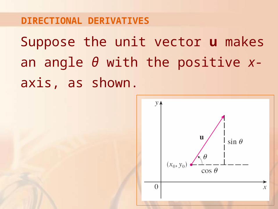
Suppose the unit vector u makes
an angle θ with the positive x-axis, as
shown.
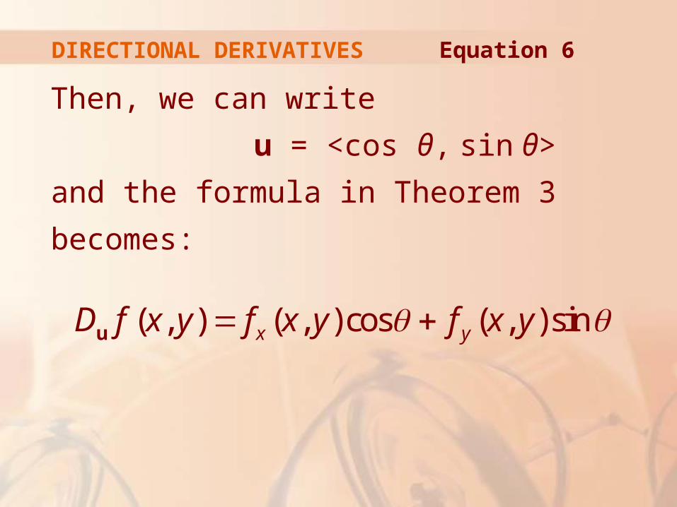
DIRECTIONAL DERIVATIVES
Then, we can write
u = <cos θ, sin θ>
and the formula in Theorem 3
becomes:
Equation 6
( , ) ( , ) cos ( , )sinx yD f x y f x y f x y u
DIRECTIONAL DERIVATIVES
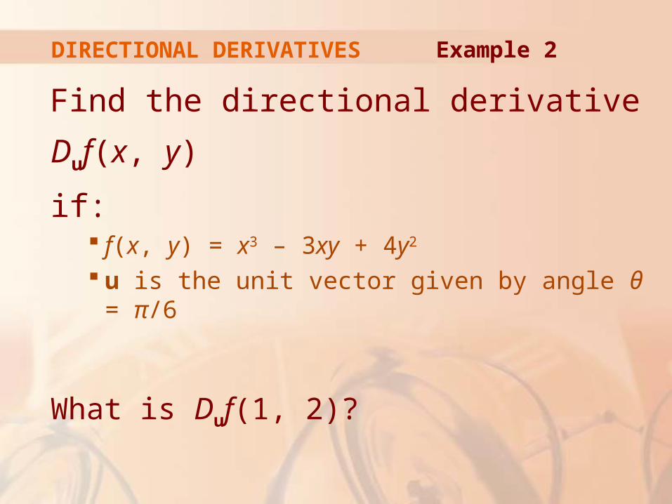
Find the directional derivative Duf(x, y)
if: f(x, y) = x3 – 3xy + 4y2
u is the unit vector given by angle θ = π/6
What is Duf(1, 2)?
Example 2
DIRECTIONAL DERIVATIVES
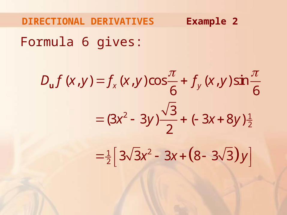
Formula 6 gives:
Example 2
2 12
212
( , ) ( , ) cos ( , )sin6 6
3(3 3 ) ( 3 8 )
2
3 3 3 8 3 3
x yD f x y f x y f x y
x y x y
x x y
u
DIRECTIONAL DERIVATIVES
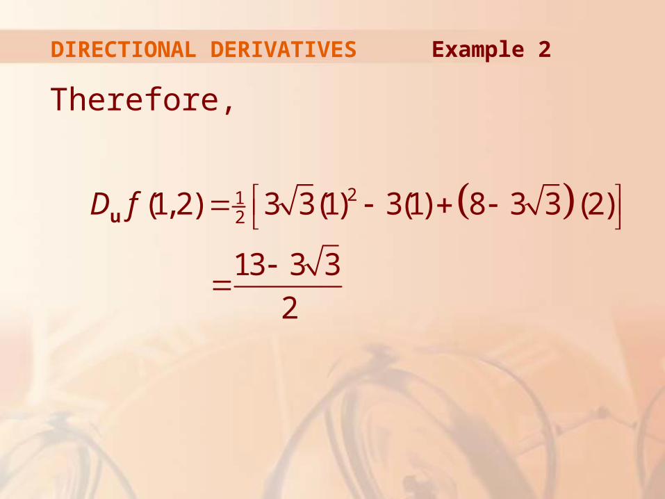
Therefore,
Example 2
212(1,2) 3 3(1) 3(1) 8 3 3 (2)
13 3 3
2
D fu
DIRECTIONAL DERIVATIVES
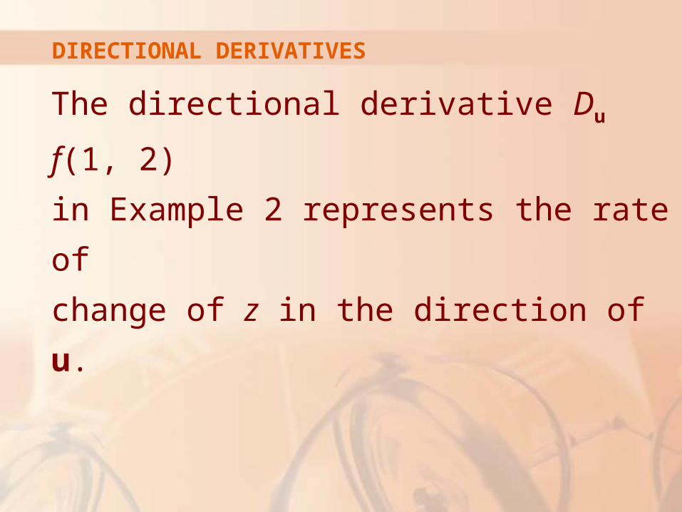
The directional derivative Du f(1, 2)
in Example 2 represents the rate of
change of z in the direction of u.

DIRECTIONAL DERIVATIVES
This is the slope of the tangent line to
the curve of intersection of the surface
z = x3 – 3xy + 4y2
and the vertical
plane through
(1, 2, 0) in the
direction of u
shown here.
THE GRADIENT VECTOR
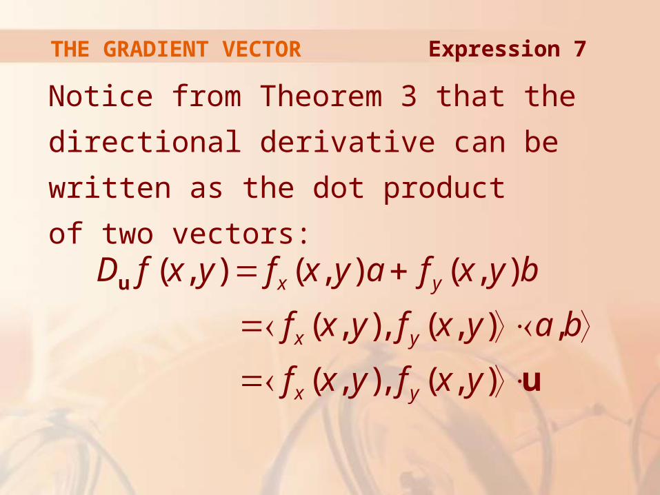
Notice from Theorem 3 that the directional
derivative can be written as the dot product
of two vectors:
( , ) ( , ) ( , )
( , ), ( , ) ,
( , ), ( , )
x y
x y
x y
D f x y f x y a f x y b
f x y f x y a b
f x y f x y
u
u
Expression 7
THE GRADIENT VECTOR
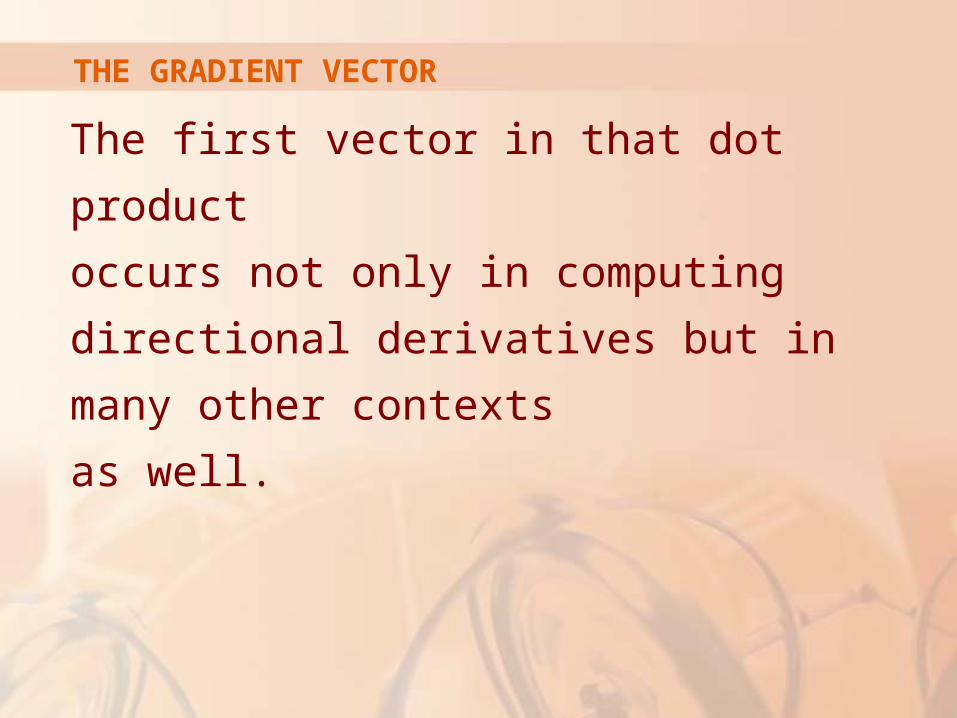
The first vector in that dot product
occurs not only in computing directional
derivatives but in many other contexts
as well.
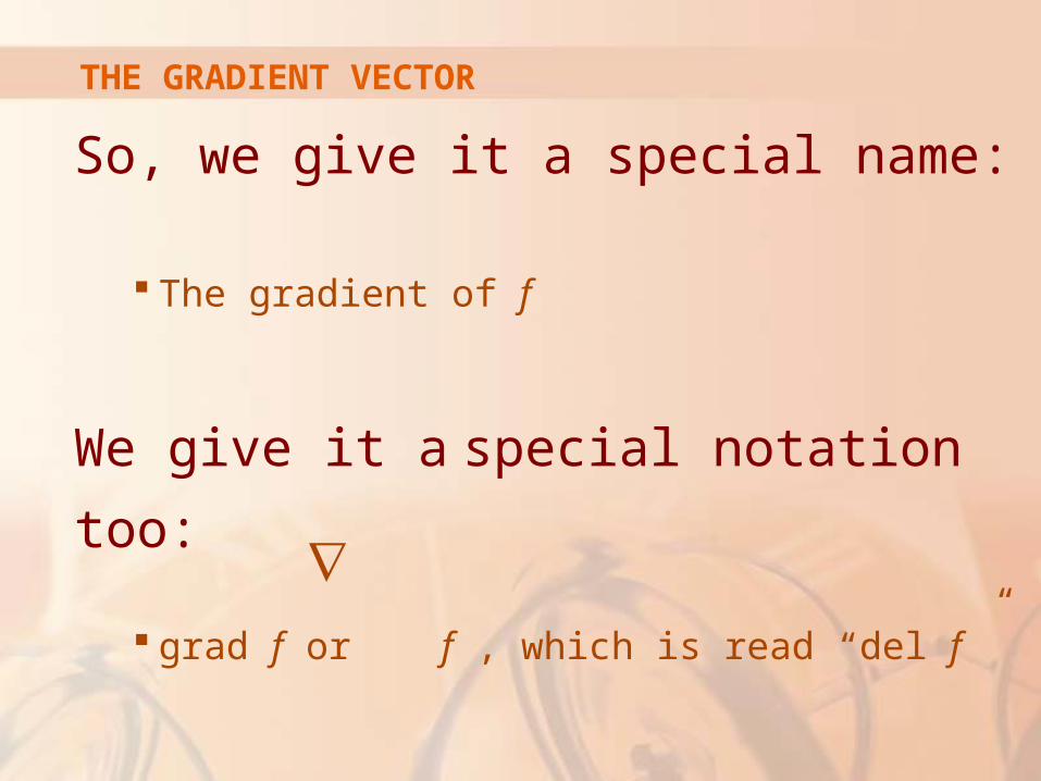
THE GRADIENT VECTOR
So, we give it a special name:
The gradient of f
We give it a special notation too:
grad f or f , which is read “del f ”
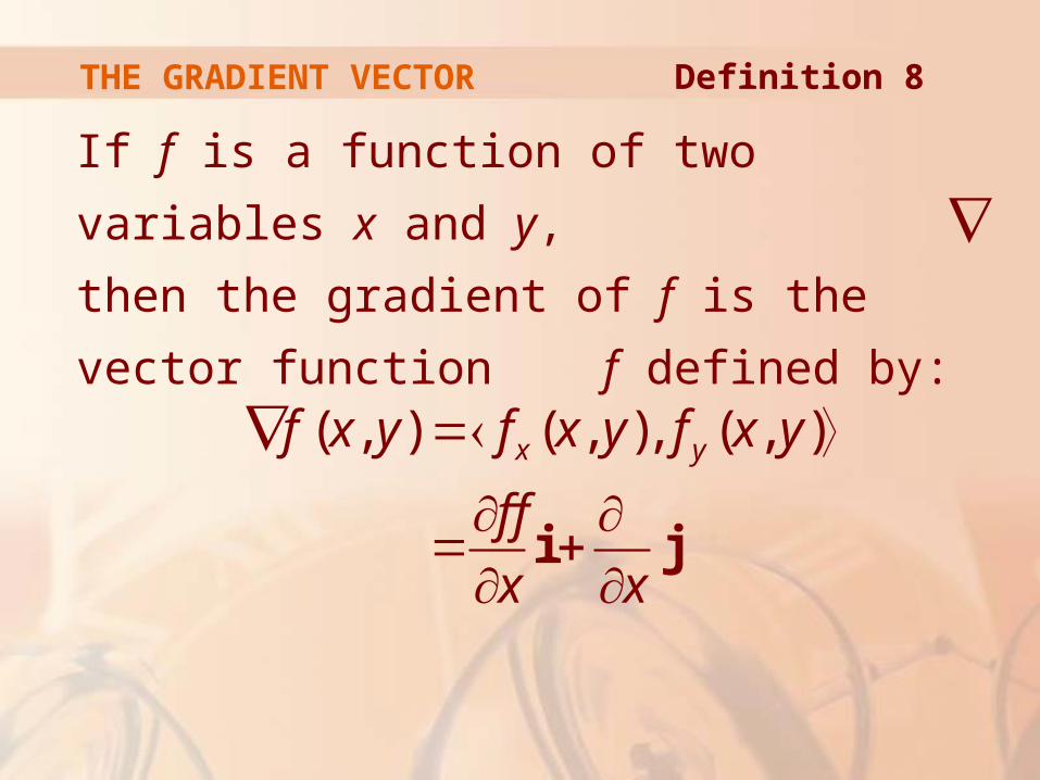
THE GRADIENT VECTOR
If f is a function of two variables x and y,
then the gradient of f is the vector function f
defined by:
Definition 8
( , ) ( , ), ( , )x yf x y f x y f x y
f f
x x
i j
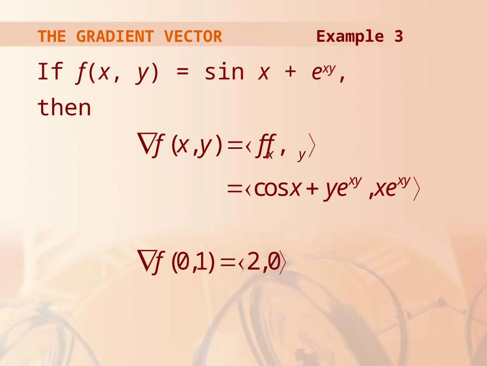
THE GRADIENT VECTOR
If f(x, y) = sin x + exy,
then
Example 3
( , ) ,
cos ,
(0,1) 2,0
x y
xy xy
f x y f f
x ye xe
f
THE GRADIENT VECTOR
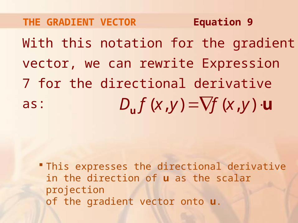
With this notation for the gradient vector, we
can rewrite Expression 7 for the directional
derivative as:
This expresses the directional derivative in the direction of u as the scalar projection of the gradient vector onto u.
Equation 9
( , ) ( , )D f x y f x y u u
THE GRADIENT VECTOR
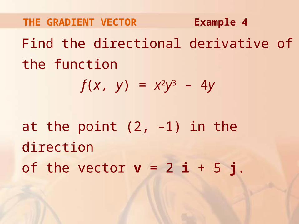
Find the directional derivative of the function
f(x, y) = x2y3 – 4y
at the point (2, –1) in the direction
of the vector v = 2 i + 5 j.
Example 4
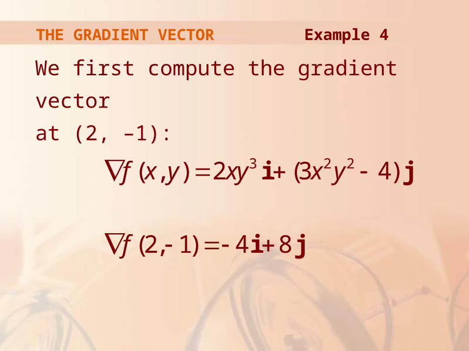
THE GRADIENT VECTOR
We first compute the gradient vector
at (2, –1):
Example 4
3 2 2( , ) 2 (3 4)
(2, 1) 4 8
f x y xy x y
f
i j
i j
THE GRADIENT VECTOR
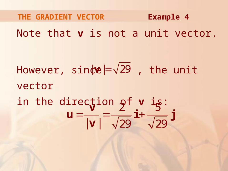
Note that v is not a unit vector.
However, since , the unit vector
in the direction of v is:
Example 4
| | 29v
2 5
| | 29 29 v
u i jv
THE GRADIENT VECTOR
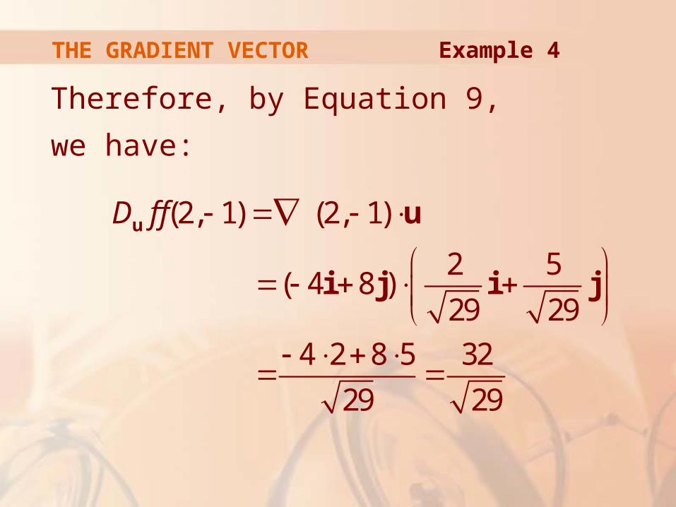
Therefore, by Equation 9,
we have:
Example 4
(2, 1) (2, 1)
2 5( 4 8 )
29 29
4 2 8 5 32
29 29
D f f
u u
i j i j
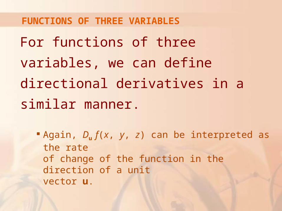
FUNCTIONS OF THREE VARIABLES
For functions of three variables, we can
define directional derivatives in a similar
manner.
Again, Du f(x, y, z) can be interpreted as the rate of change of the function in the direction of a unit vector u.
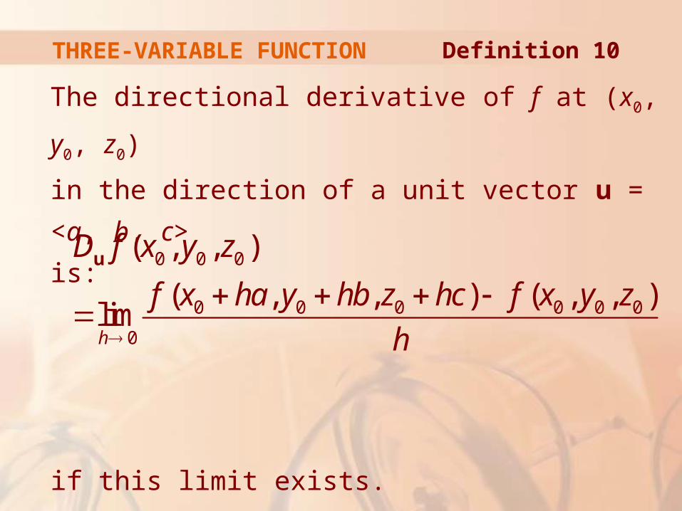
The directional derivative of f at (x0, y0, z0)
in the direction of a unit vector u = <a, b, c>
is:
if this limit exists.
THREE-VARIABLE FUNCTION Definition 10
0 0 0
0 0 0 0 0 0
0
( , , )
( , , ) ( , , )limh
D f x y z
f x ha y hb z hc f x y z
h
u
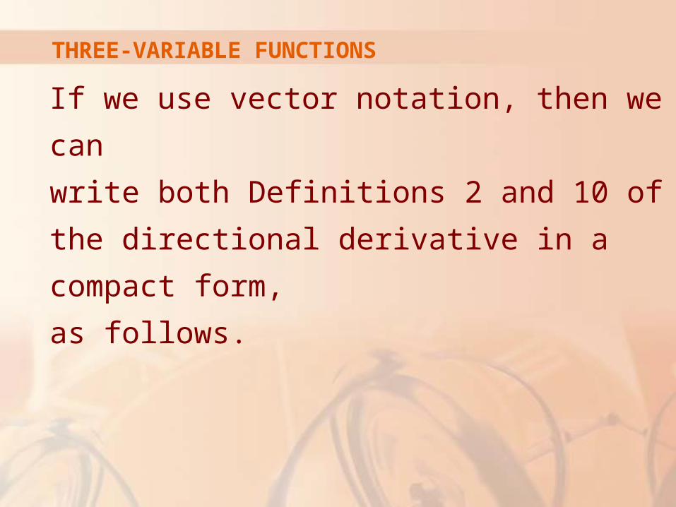
If we use vector notation, then we can
write both Definitions 2 and 10 of the
directional derivative in a compact form,
as follows.
THREE-VARIABLE FUNCTIONS
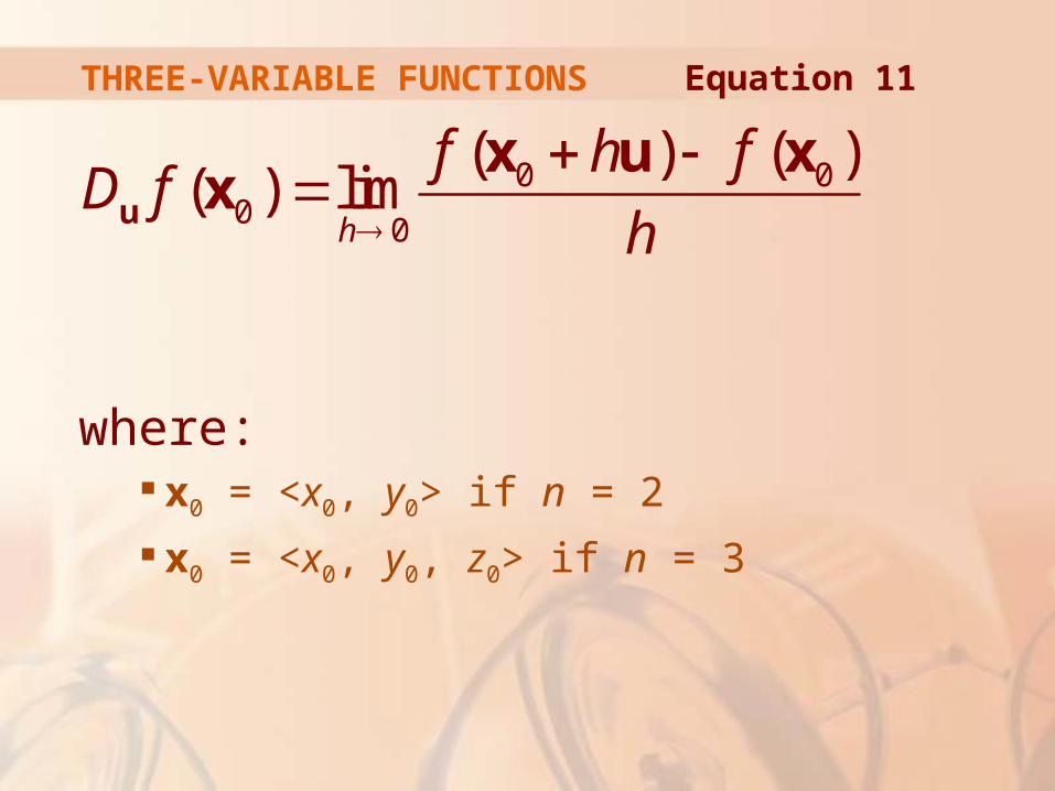
THREE-VARIABLE FUNCTIONS Equation 11
0 00
0
( ) ( )( ) lim
h
f h fD f
h
u
x u xx
where: x0 = <x0, y0> if n = 2
x0 = <x0, y0, z0> if n = 3
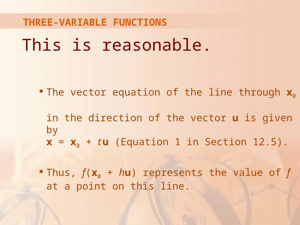
This is reasonable.
The vector equation of the line through x0 in the direction of the vector u is given by x = x0 + t u (Equation 1 in Section 12.5).
Thus, f(x0 + hu) represents the value of f at a point on this line.
THREE-VARIABLE FUNCTIONS
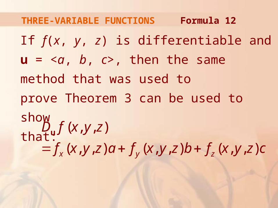
If f(x, y, z) is differentiable and u = <a, b, c>,
then the same method that was used to
prove Theorem 3 can be used to show
that:
THREE-VARIABLE FUNCTIONS Formula 12
( , , )
( , , ) ( , , ) ( , , )x y z
D f x y z
f x y z a f x y z b f x y z c u
THREE-VARIABLE FUNCTIONS
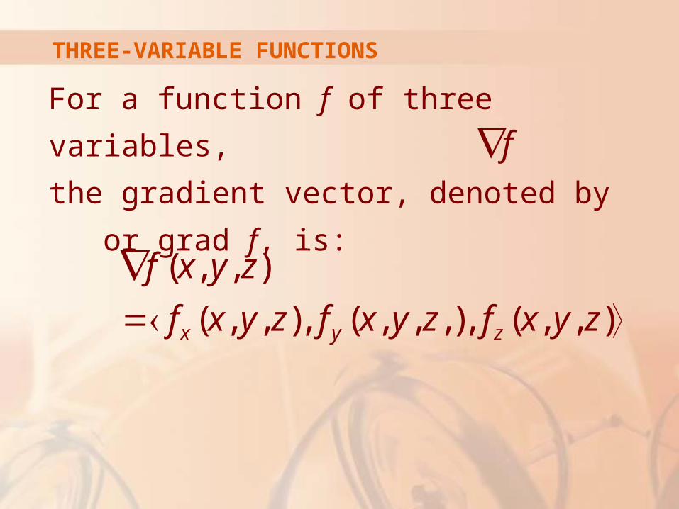
For a function f of three variables,
the gradient vector, denoted by or grad f,
is:
f
( , , )
( , , ), ( , , , ), ( , , )x y z
f x y z
f x y z f x y z f x y z
THREE-VARIABLE FUNCTIONS
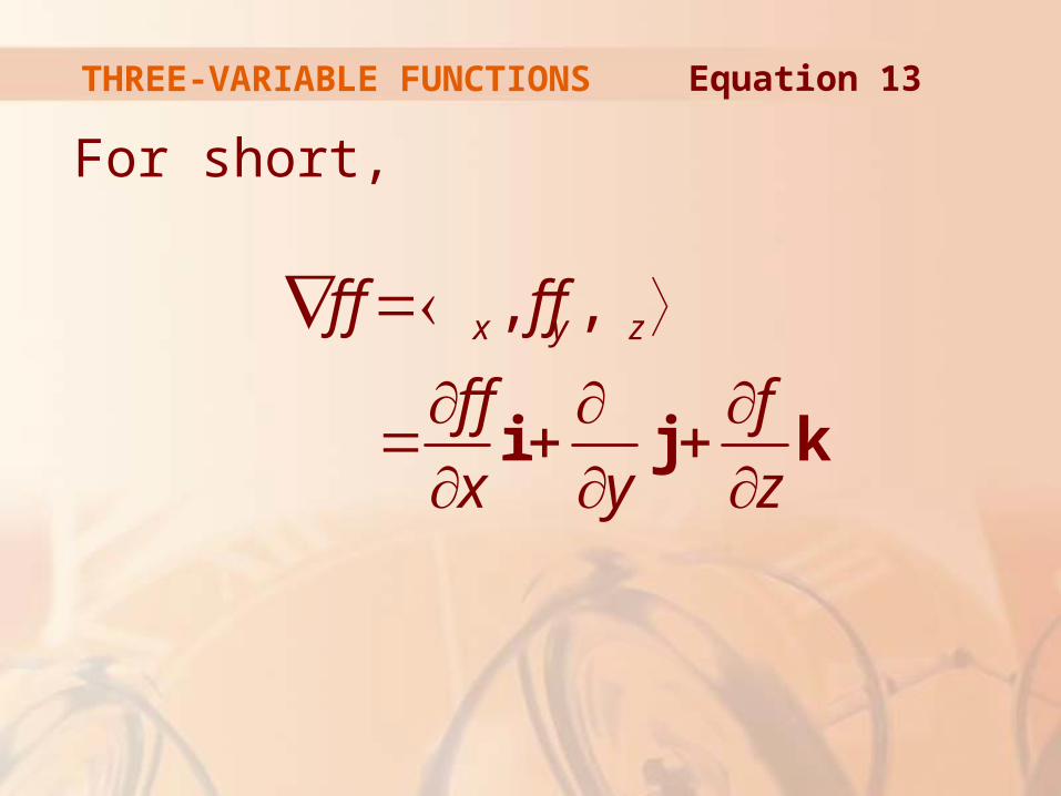
For short,
, ,x y zf f f f
f f f
x y z
i j k
Equation 13
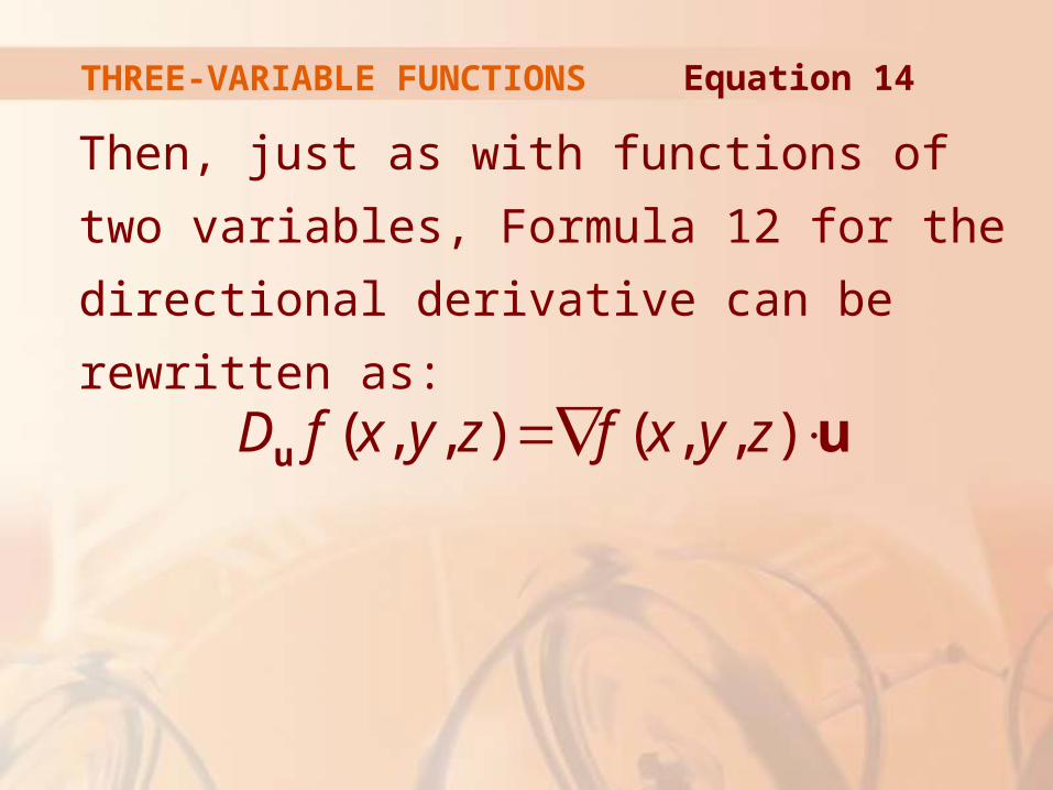
THREE-VARIABLE FUNCTIONS
Then, just as with functions of two variables,
Formula 12 for the directional derivative can
be rewritten as:
( , , ) ( , , )D f x y z f x y z u u
Equation 14
THREE-VARIABLE FUNCTIONS
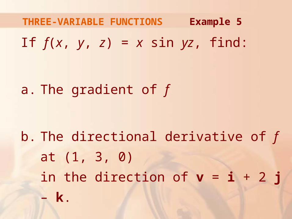
If f(x, y, z) = x sin yz, find:
a. The gradient of f
b. The directional derivative of f at (1, 3, 0)
in the direction of v = i + 2 j – k.
Example 5
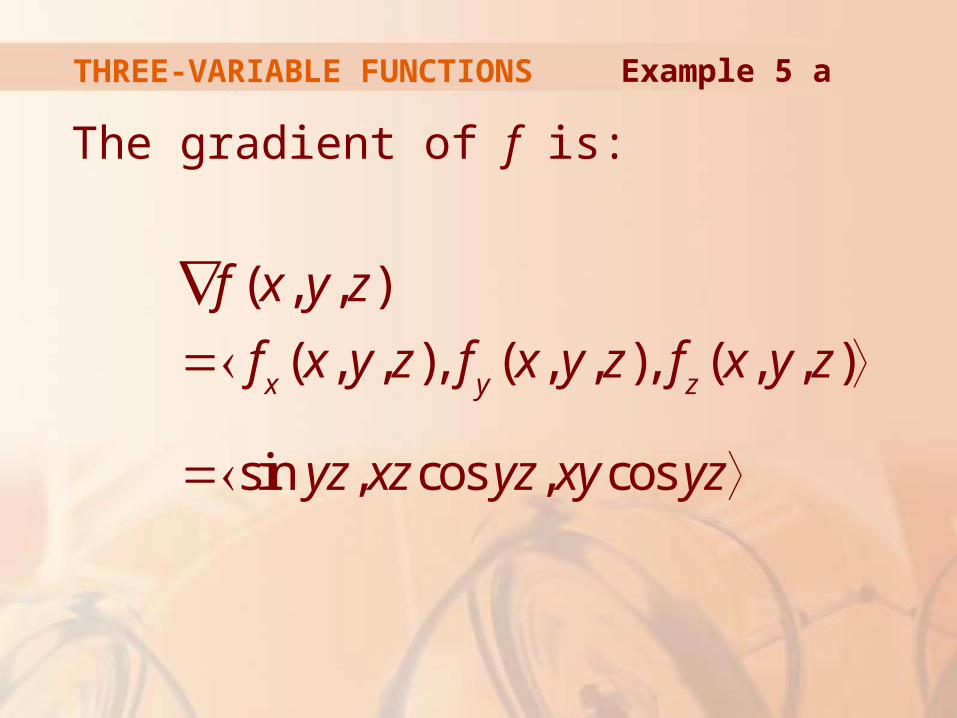
THREE-VARIABLE FUNCTIONS
The gradient of f is:
Example 5 a
f (x, y, z)
fx(x, y, z), f
y(x, y, z), f
z(x, y, z)
sin yz,xz cos yz,xycos yz
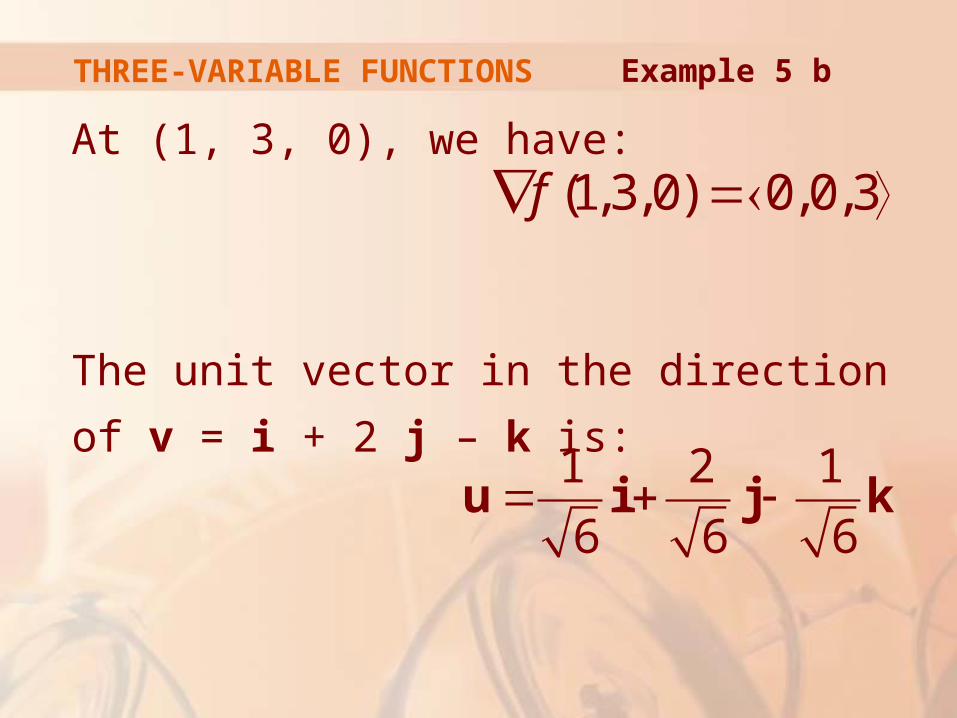
THREE-VARIABLE FUNCTIONS
At (1, 3, 0), we have:
The unit vector in the direction
of v = i + 2 j – k is:
Example 5 b
(1,3,0) 0,0,3f
1 2 1
6 6 6 u i j k
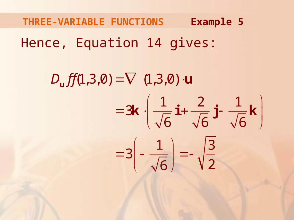
THREE-VARIABLE FUNCTIONS
Hence, Equation 14 gives:
Example 5
(1,3,0) (1,3,0)
1 2 13
6 6 6
1 33
26
D f f
u u
k i j k
MAXIMIZING THE DIRECTIONAL DERIVATIVE
Suppose we have a function f of two or three
variables and we consider all possible
directional derivatives of f at a given point.
These give the rates of change of f in all possible directions.
MAXIMIZING THE DIRECTIONAL DERIVATIVE
We can then ask the questions:
In which of these directions does f change fastest?
What is the maximum rate of change?
The answers are provided by
the following theorem.
MAXIMIZING THE DIRECTIONAL DERIVATIVE
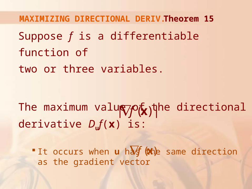
Suppose f is a differentiable function of
two or three variables.
The maximum value of the directional
derivative Duf(x) is:
It occurs when u has the same direction as the gradient vector
MAXIMIZING DIRECTIONAL DERIV. Theorem 15
| ( ) |f x
( )f x
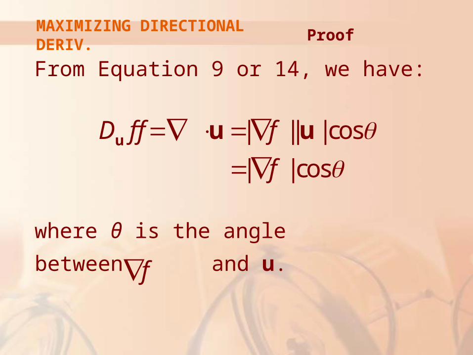
From Equation 9 or 14, we have:
where θ is the angle
between and u.
MAXIMIZING DIRECTIONAL DERIV. Proof
| || | cos
| | cos
D f f f
f
u u u
f
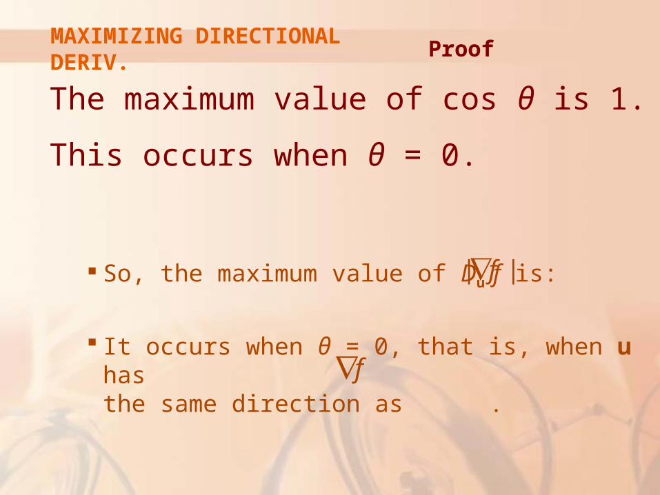
The maximum value of cos θ is 1.
This occurs when θ = 0.
So, the maximum value of Du f is:
It occurs when θ = 0, that is, when u has the same direction as .
MAXIMIZING DIRECTIONAL DERIV. Proof
| |f
f
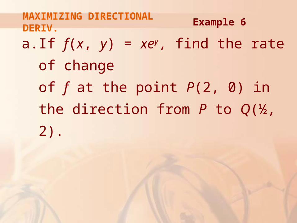
a. If f(x, y) = xey, find the rate of change
of f at the point P(2, 0) in the direction
from P to Q(½, 2).
MAXIMIZING DIRECTIONAL DERIV. Example 6
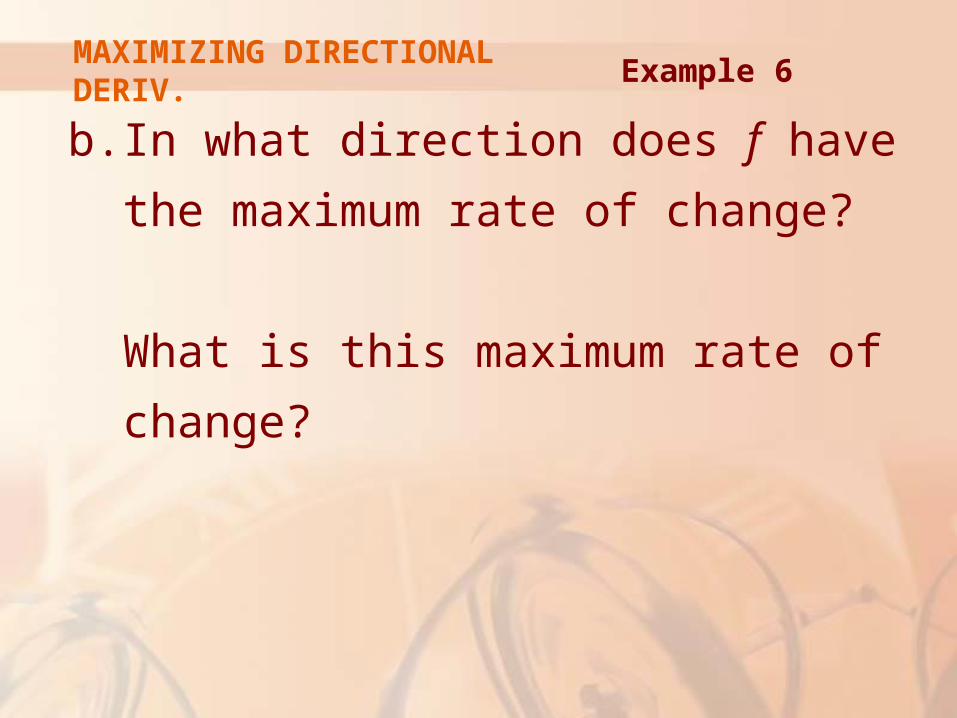
b. In what direction does f have
the maximum rate of change?
What is this maximum rate of change?
MAXIMIZING DIRECTIONAL DERIV. Example 6
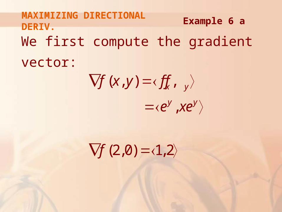
We first compute the gradient vector:
MAXIMIZING DIRECTIONAL DERIV. Example 6 a
( , ) ,
,
(2,0) 1,2
x y
y y
f x y f f
e xe
f
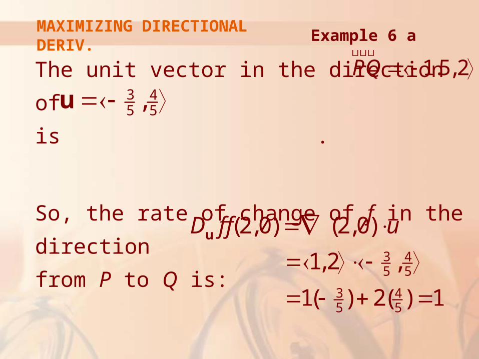
The unit vector in the direction of
is .
So, the rate of change of f in the direction
from P to Q is:
MAXIMIZING DIRECTIONAL DERIV. Example 6 a
1.5,2PQ ��������������
3 45 5, u
3 45 5
3 45 5
(2,0) (2,0)
1,2 ,
1( ) 2( ) 1
D f f u
u
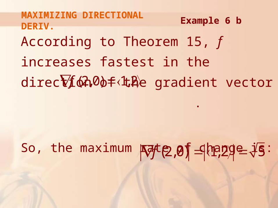
According to Theorem 15, f increases
fastest in the direction of the gradient vector
.
So, the maximum rate of change is:
MAXIMIZING DIRECTIONAL DERIV. Example 6 b
(2,0) 1,2f
(2,0) 1,2 5f
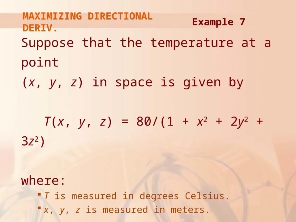
Suppose that the temperature at a point
(x, y, z) in space is given by
T(x, y, z) = 80/(1 + x2 + 2y2 + 3z2)
where: T is measured in degrees Celsius. x, y, z is measured in meters.
MAXIMIZING DIRECTIONAL DERIV. Example 7
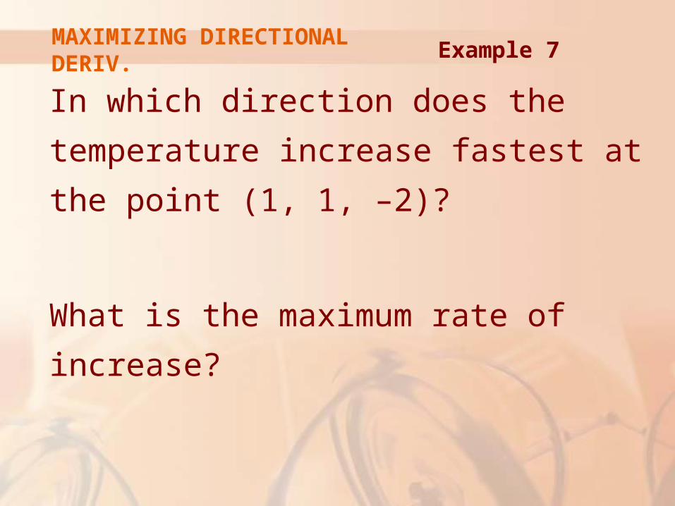
In which direction does the temperature
increase fastest at the point (1, 1, –2)?
What is the maximum rate of increase?
MAXIMIZING DIRECTIONAL DERIV. Example 7
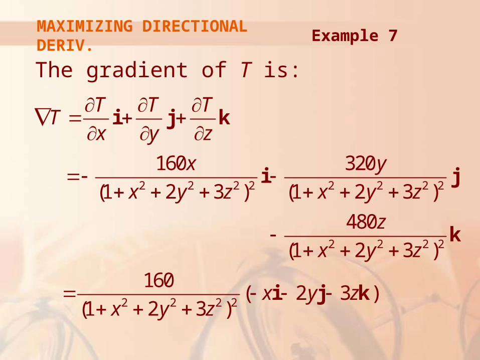
MAXIMIZING DIRECTIONAL DERIV.
The gradient of T is:
Example 7
2 2 2 2 2 2 2 2
2 2 2 2
2 2 2 2
160 320
(1 2 3 ) (1 2 3 )
480
(1 2 3 )
160( 2 3 )
(1 2 3 )
T T TT
x y z
x y
x y z x y z
z
x y z
x y zx y z
i j k
i j
k
i j k
MAXIMIZING DIRECTIONAL DERIV.
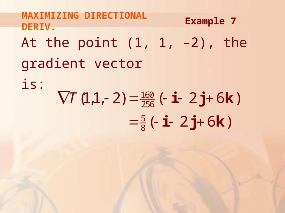
At the point (1, 1, –2), the gradient vector
is:
Example 7
160256
58
(1,1, 2) ( 2 6 )
( 2 6 )
T
i j k
i j k
MAXIMIZING DIRECTIONAL DERIV.
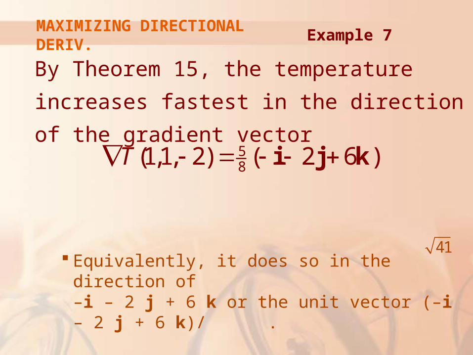
By Theorem 15, the temperature increases
fastest in the direction of the gradient vector
Equivalently, it does so in the direction of –i – 2 j + 6 k or the unit vector (–i – 2 j + 6 k)/ .
Example 7
58(1,1, 2) ( 2 6 )T i j k
41
MAXIMIZING DIRECTIONAL DERIV.
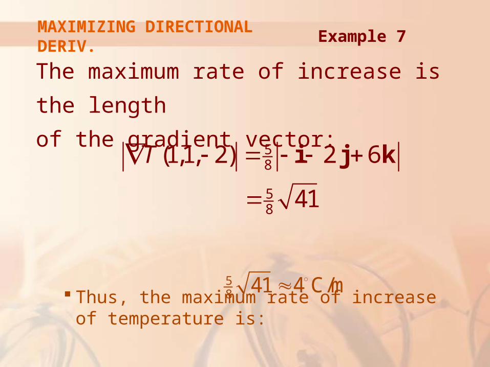
The maximum rate of increase is the length
of the gradient vector:
Thus, the maximum rate of increase of temperature is:
Example 7
58
58
(1,1, 2) 2 6
41
T
i j k
58 41 4 C/m
TANGENT PLANES TO LEVEL SURFACES
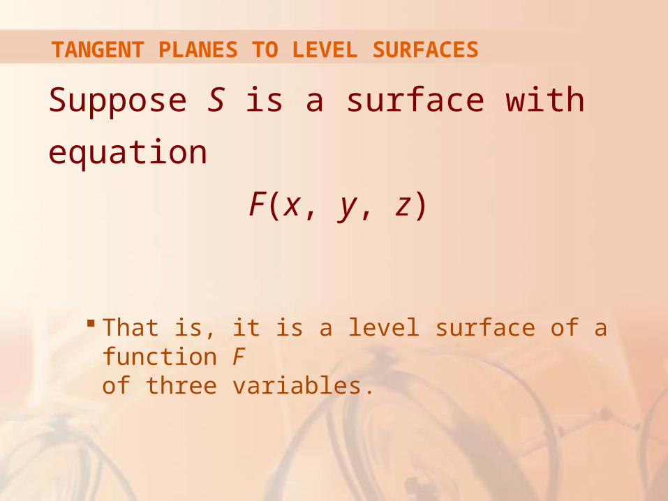
Suppose S is a surface with
equation
F(x, y, z)
That is, it is a level surface of a function F of three variables.
TANGENT PLANES TO LEVEL SURFACES
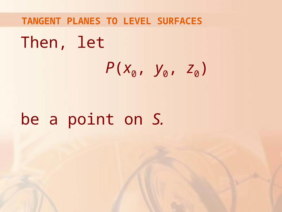
Then, let
P(x0, y0, z0)
be a point on S.
Then, let C be any curve that lies on
the surface S and passes through
the point P.
Recall from Section 13.1 that the curve C is described by a continuous vector function
r(t) = <x(t), y(t), z(t)>
TANGENT PLANES TO LEVEL SURFACES
Let t0 be the parameter value
corresponding to P.
That is, r(t0) = <x0, y0, z0>
TANGENT PLANES TO LEVEL SURFACES
Since C lies on S, any point (x(t), y(t), z(t))
must satisfy the equation of S.
That is,
F(x(t), y(t), z(t)) = k
Equation 16TANGENT PLANES
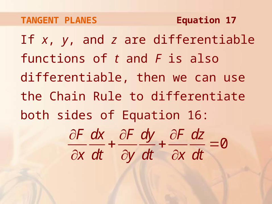
If x, y, and z are differentiable functions of t
and F is also differentiable, then we can use
the Chain Rule to differentiate both sides of
Equation 16:
TANGENT PLANES
0F dx F dy F dz
x dt y dt x dt
Equation 17
However, as
and
Equation 17 can be written in terms
of a dot product as:
TANGENT PLANES
'( ) 0F t r
, ,x y zF F F F
'( ) '( ), '( ), '( )t x t y t z t r
TANGENT PLANES
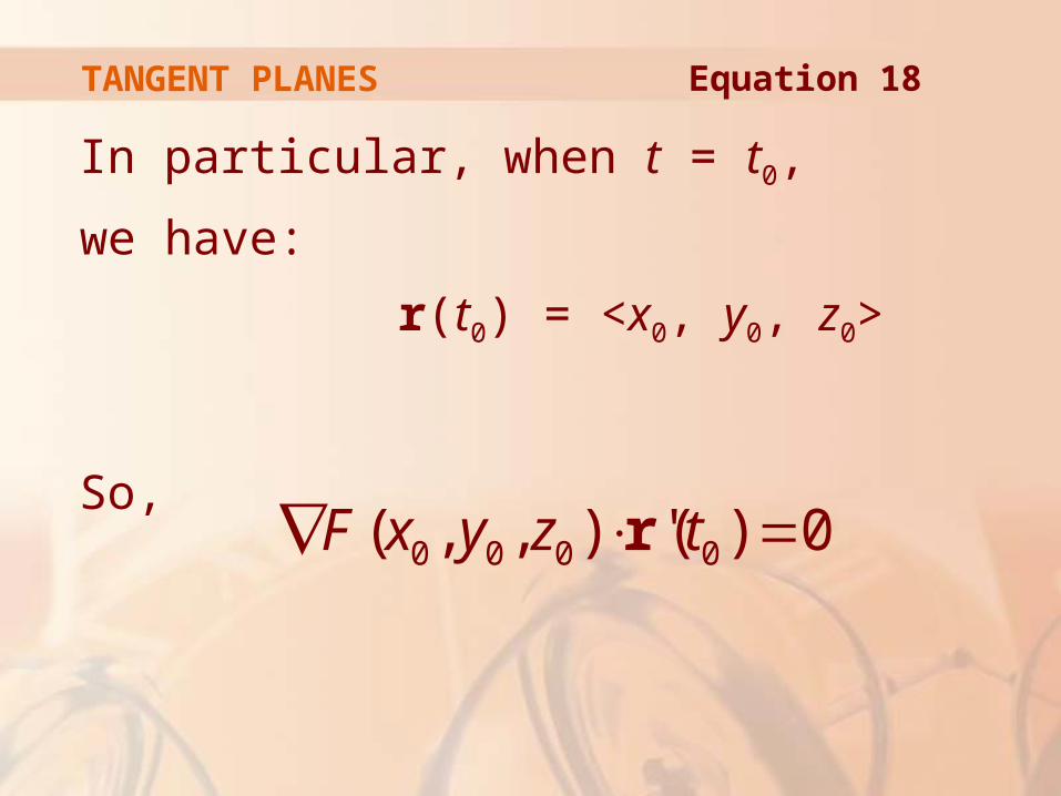
In particular, when t = t0,
we have:
r(t0) = <x0, y0, z0>
So, 0 0 0 0( , , ) '( ) 0F x y z t r
Equation 18
TANGENT PLANES
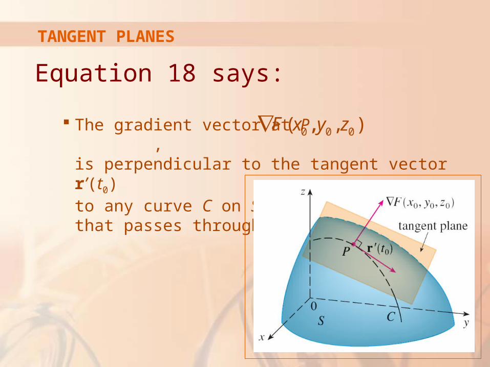
Equation 18 says:
The gradient vector at P, , is perpendicular to the tangent vector r’(t0) to any curve C on S that passes through P.
0 0 0( , , )F x y z
TANGENT PLANES
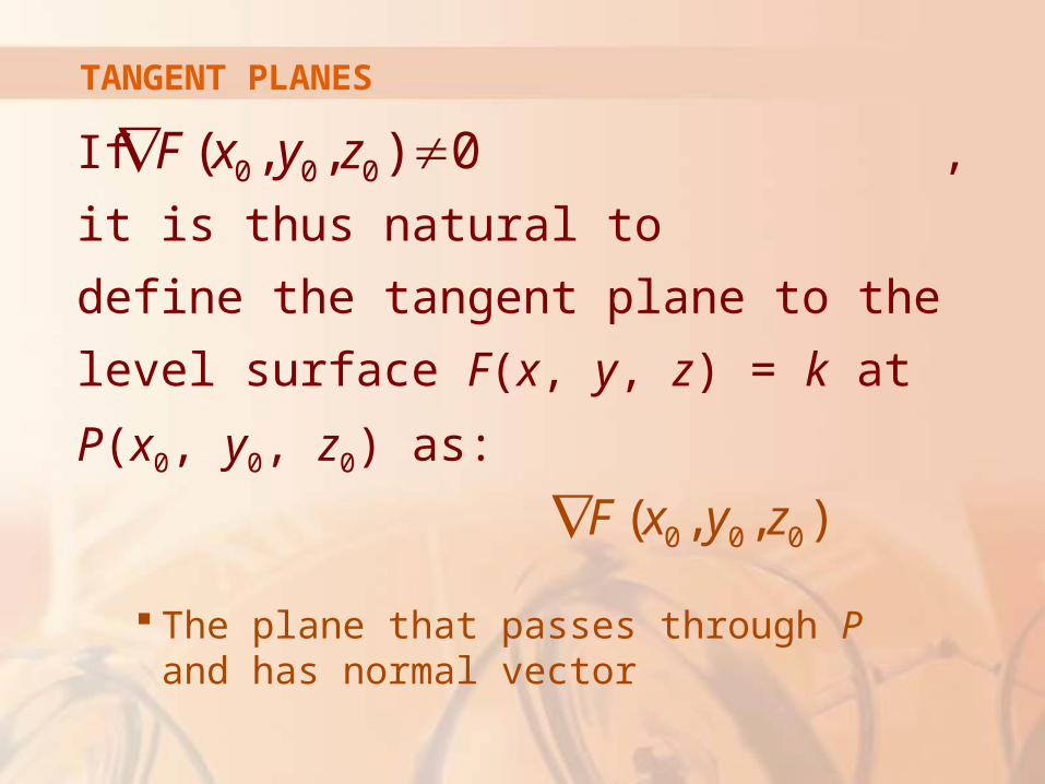
If , it is thus natural to
define the tangent plane to the level surface
F(x, y, z) = k at P(x0, y0, z0) as:
The plane that passes through P and has normal vector
0 0 0( , , ) 0F x y z
0 0 0( , , )F x y z
TANGENT PLANES
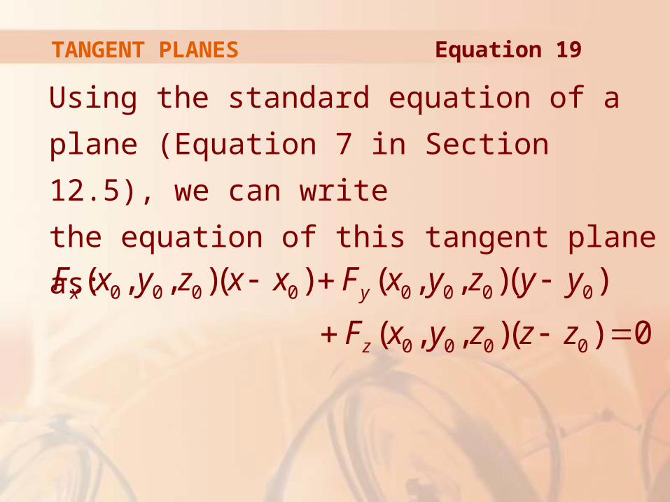
Using the standard equation of a plane
(Equation 7 in Section 12.5), we can write
the equation of this tangent plane as:
0 0 0 0 0 0 0 0
0 0 0 0
( , , )( ) ( , , )( )
( , , )( ) 0
x y
z
F x y z x x F x y z y y
F x y z z z
Equation 19
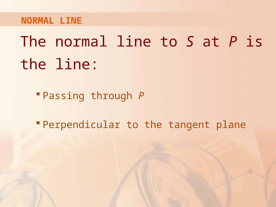
NORMAL LINE
The normal line to S at P is
the line:
Passing through P
Perpendicular to the tangent plane
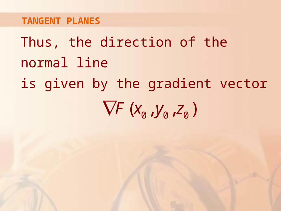
TANGENT PLANES
Thus, the direction of the normal line
is given by the gradient vector
0 0 0( , , )F x y z
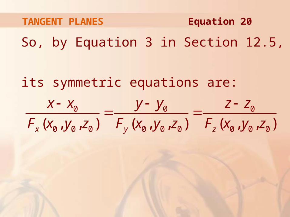
TANGENT PLANES
So, by Equation 3 in Section 12.5,
its symmetric equations are:
Equation 20
0 0 0
0 0 0 0 0 0 0 0 0( , , ) ( , , ) ( , , )x y z
x x y y z z
F x y z F x y z F x y z
TANGENT PLANES
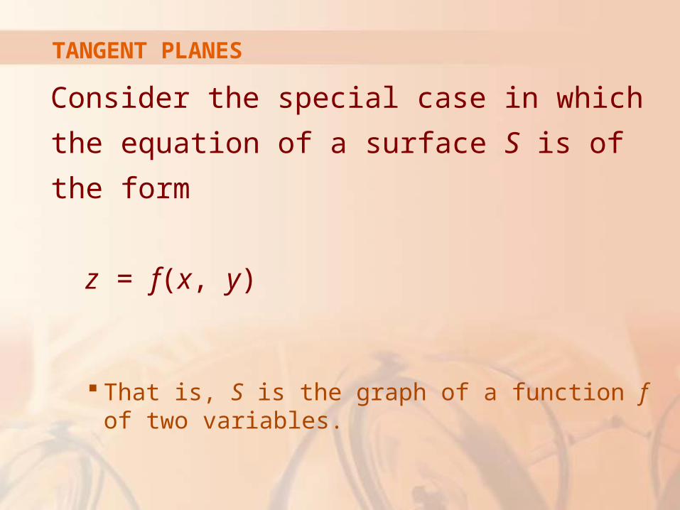
Consider the special case in which
the equation of a surface S is of the form
z = f(x, y)
That is, S is the graph of a function f of two variables.
TANGENT PLANES
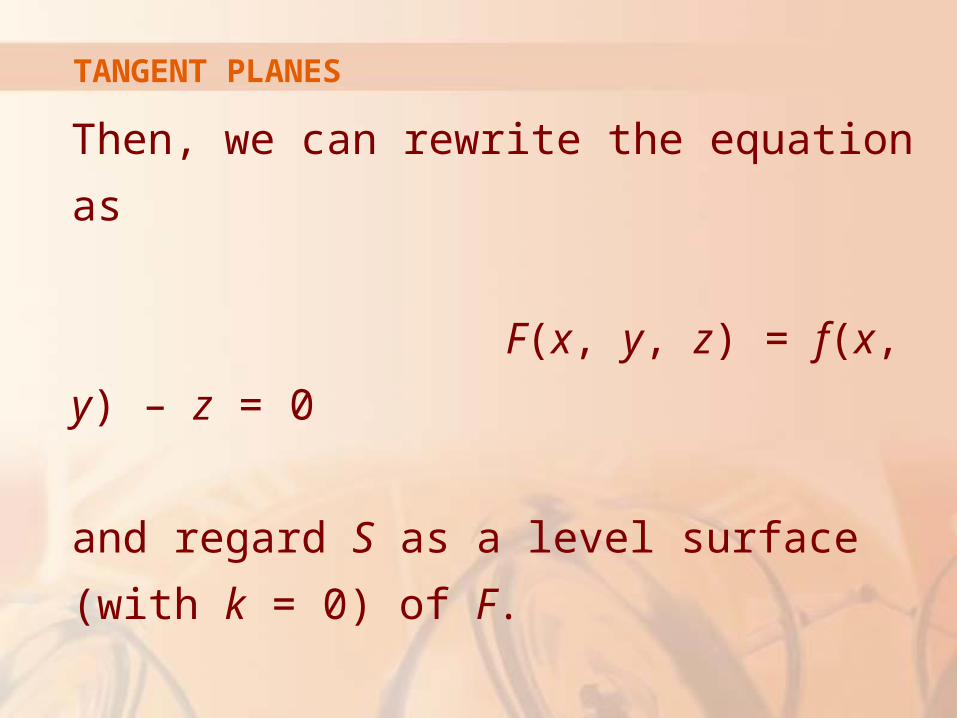
Then, we can rewrite the equation as
F(x, y, z) = f(x, y) – z = 0
and regard S as a level surface
(with k = 0) of F.
TANGENT PLANES
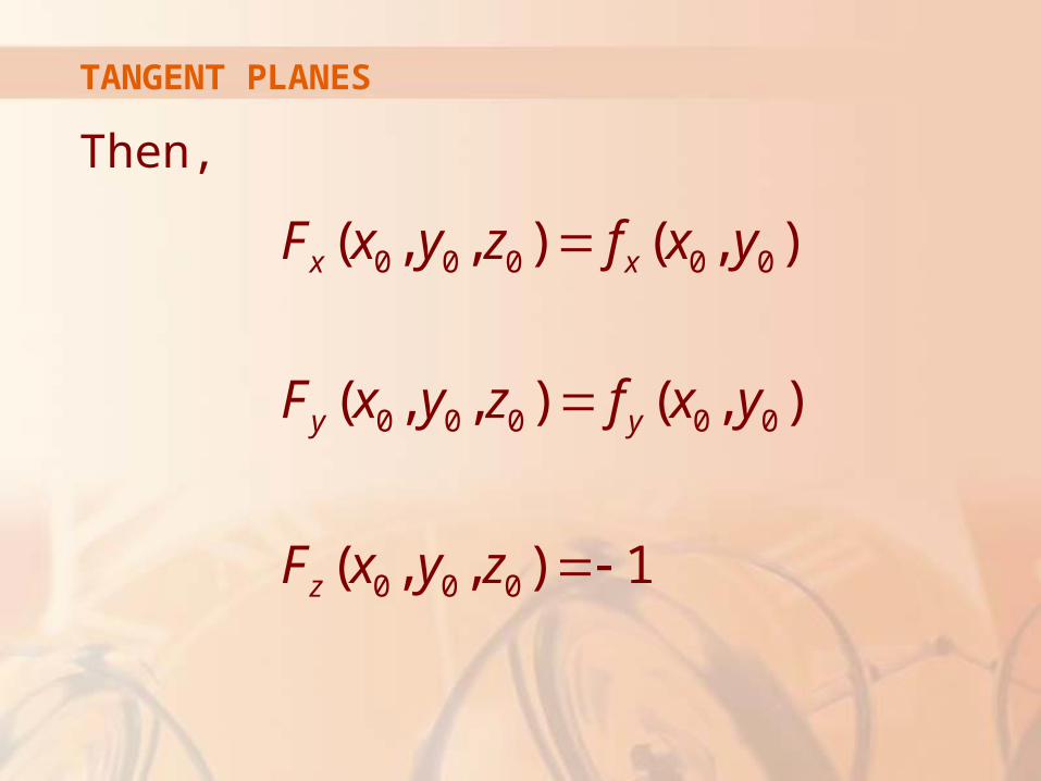
Then,
0 0 0 0 0
0 0 0 0 0
0 0 0
( , , ) ( , )
( , , ) ( , )
( , , ) 1
x x
y y
z
F x y z f x y
F x y z f x y
F x y z
TANGENT PLANES
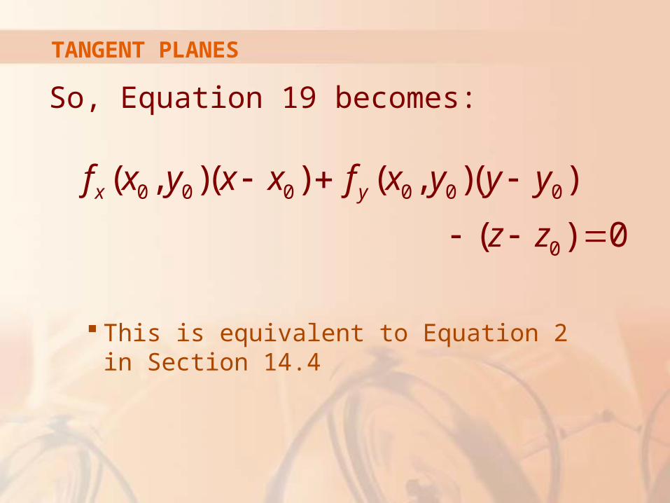
So, Equation 19 becomes:
This is equivalent to Equation 2 in Section 14.4
0 0 0 0 0 0
0
( , )( ) ( , )( )
( ) 0
x yf x y x x f x y y y
z z
TANGENT PLANES
Thus, our new, more general, definition
of a tangent plane is consistent with
the definition that was given for the special
case of Section 14.4
TANGENT PLANES
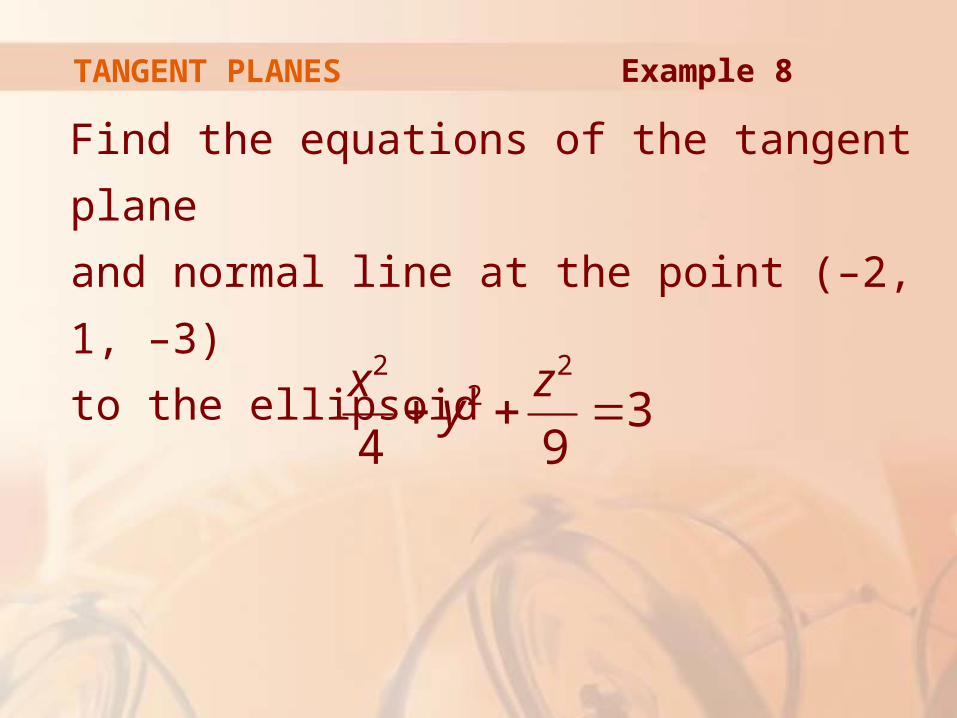
Find the equations of the tangent plane
and normal line at the point (–2, 1, –3)
to the ellipsoid
Example 8
2 22 3
4 9
x zy
TANGENT PLANES
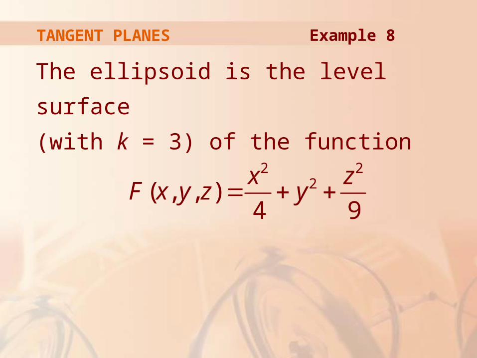
The ellipsoid is the level surface
(with k = 3) of the function
Example 8
2 22( , , )
4 9
x zF x y z y
TANGENT PLANES
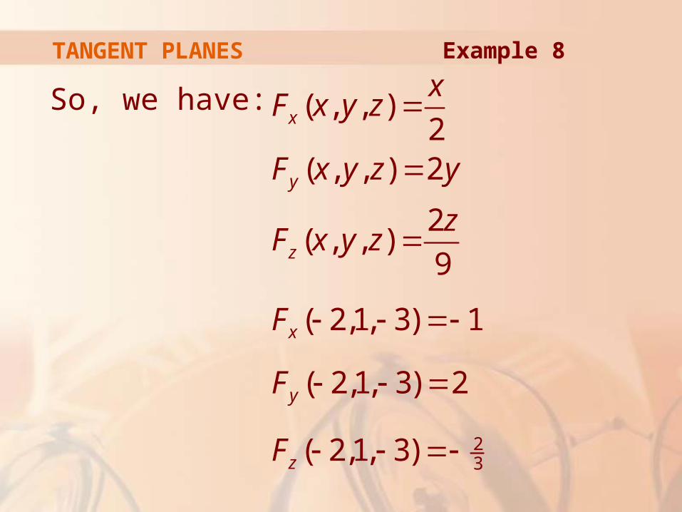
So, we have:
Example 8
23
( , , )2
( , , ) 2
2( , , )
9
( 2,1, 3) 1
( 2,1, 3) 2
( 2,1, 3)
x
y
z
x
y
z
xF x y z
F x y z y
zF x y z
F
F
F
TANGENT PLANES
Then, Equation 19 gives the equation
of the tangent plane at (–2, 1, –3)
as:
This simplifies to:
3x – 6y + 2z + 18 = 0
Example 8
231( 2) 2( 1) ( 3) 0x y z
TANGENT PLANES
By Equation 20, symmetric equations
of the normal line are:
23
2 1 3
1 2
x y z
Example 8
TANGENT PLANES
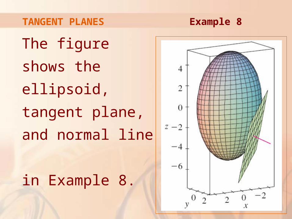
The figure shows
the ellipsoid,
tangent plane,
and normal line
in Example 8.
Example 8
SIGNIFICANCE OF GRADIENT VECTOR
We now summarize the ways
in which the gradient vector is
significant.
We first consider a function f of
three variables and a point P(x0, y0, z0)
in its domain.
SIGNIFICANCE OF GRADIENT VECTOR
On the one hand, we know from Theorem 15
that the gradient vector gives
the direction of fastest increase of f.
SIGNIFICANCE OF GRADIENT VECTOR
0 0 0( , , )f x y z
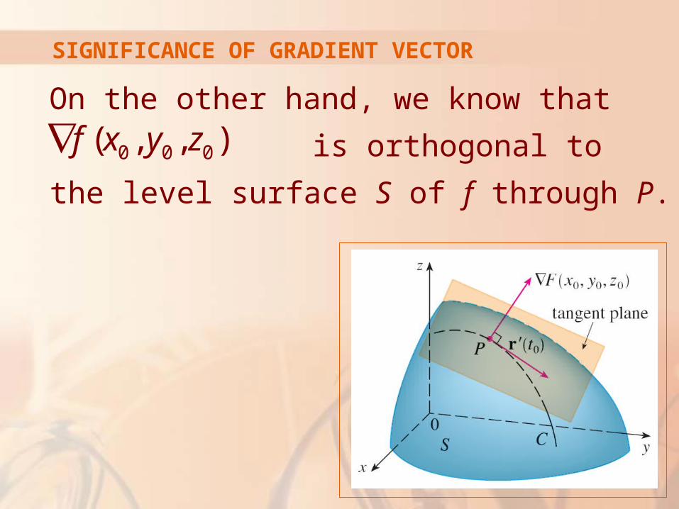
On the other hand, we know that
is orthogonal to the level
surface S of f through P.
SIGNIFICANCE OF GRADIENT VECTOR
0 0 0( , , )f x y z
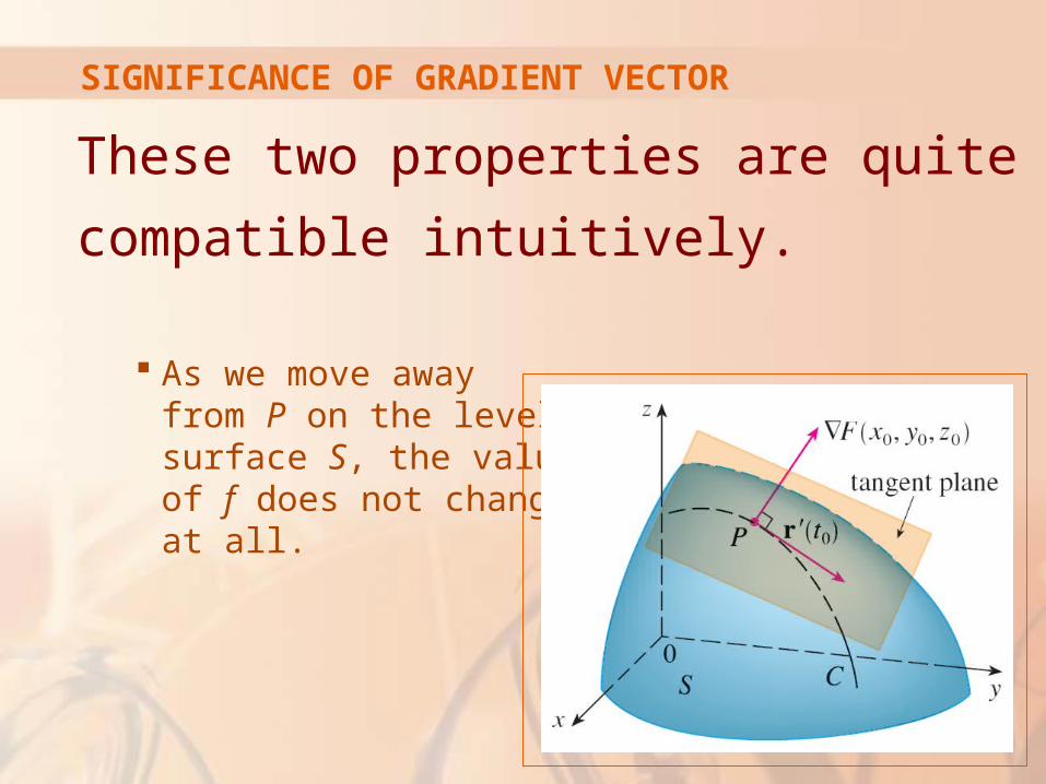
These two properties are quite
compatible intuitively.
As we move away from P on the level surface S, the value of f does not change at all.
SIGNIFICANCE OF GRADIENT VECTOR
So, it seems reasonable that, if we
move in the perpendicular direction,
we get the maximum increase.
SIGNIFICANCE OF GRADIENT VECTOR
In like manner, we consider a function f
of two variables and a point P(x0, y0)
in its domain.
SIGNIFICANCE OF GRADIENT VECTOR
Again, the gradient vector
gives the direction of fastest increase
of f.
SIGNIFICANCE OF GRADIENT VECTOR
0 0( , )f x y
Also, by considerations similar to our
discussion of tangent planes, it can be
shown that:
is perpendicular to the level curve f(x, y) = k that passes through P.
SIGNIFICANCE OF GRADIENT VECTOR
0 0( , )f x y
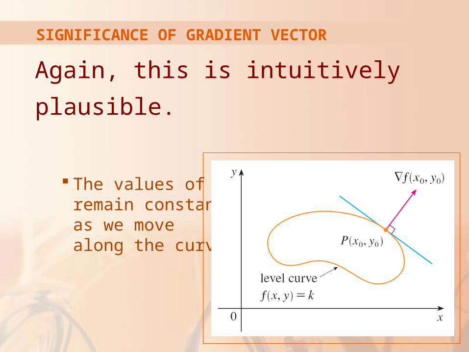
Again, this is intuitively plausible.
The values of f remain constant as we move along the curve.
SIGNIFICANCE OF GRADIENT VECTOR
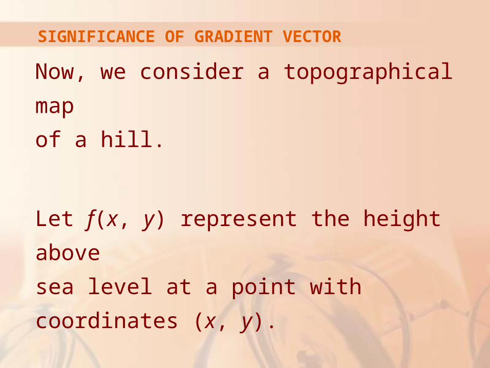
Now, we consider a topographical map
of a hill.
Let f(x, y) represent the height above
sea level at a point with coordinates (x, y).
SIGNIFICANCE OF GRADIENT VECTOR
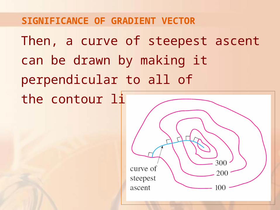
Then, a curve of steepest ascent can be
drawn by making it perpendicular to all of
the contour lines.
SIGNIFICANCE OF GRADIENT VECTOR
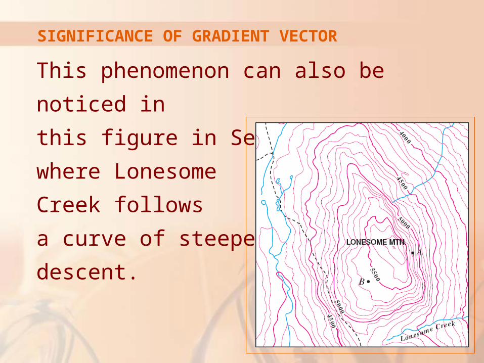
This phenomenon can also be noticed in
this figure in Section 14.1,
where Lonesome
Creek follows
a curve of steepest
descent.
SIGNIFICANCE OF GRADIENT VECTOR
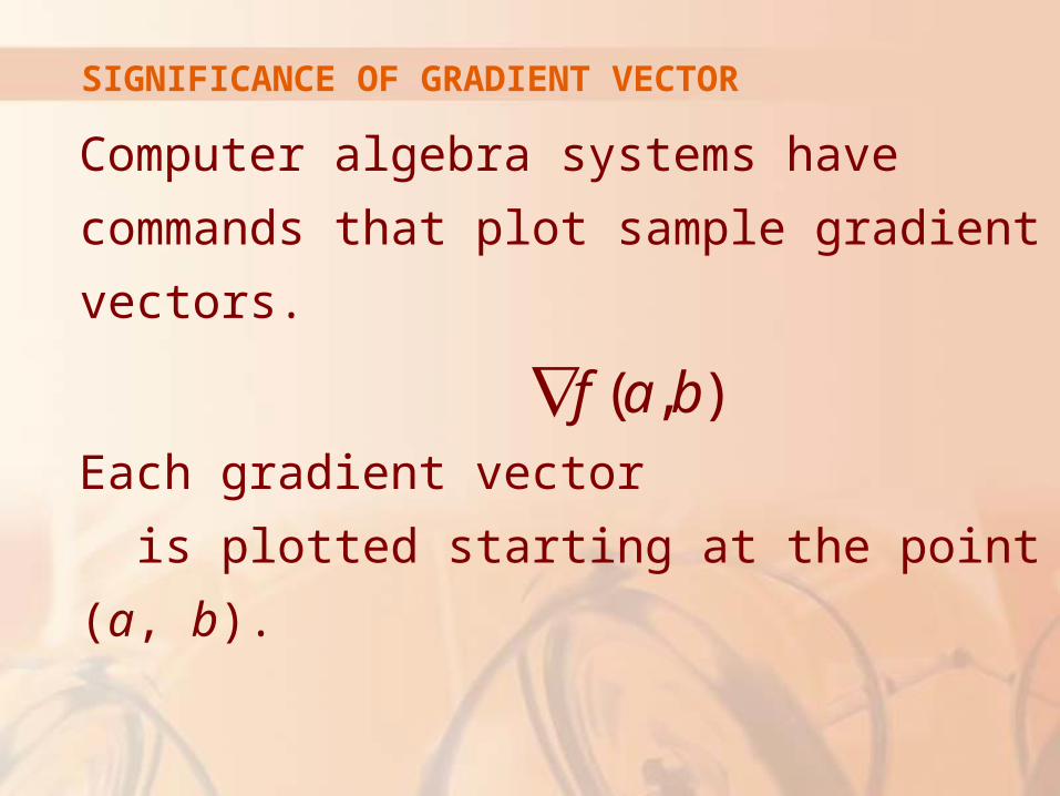
Computer algebra systems have commands
that plot sample gradient vectors.
Each gradient vector is plotted
starting at the point (a, b).
SIGNIFICANCE OF GRADIENT VECTOR
( , )f a b
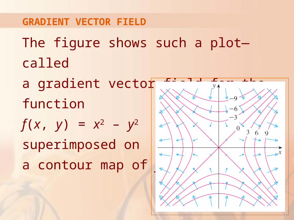
The figure shows such a plot—called
a gradient vector field—for the function
f(x, y) = x2 – y2
superimposed on
a contour map of f.
GRADIENT VECTOR FIELD
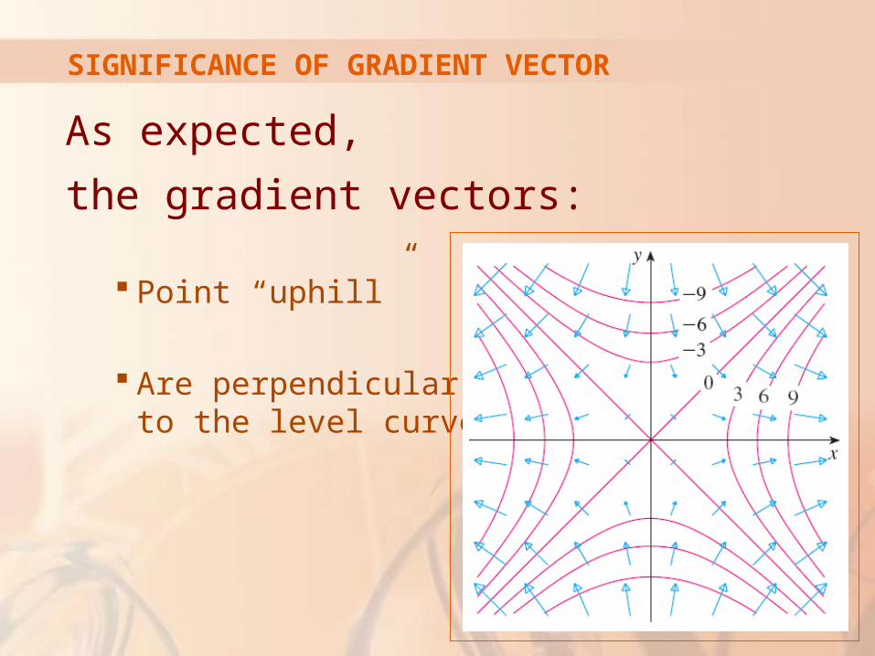
As expected,
the gradient vectors:
Point “uphill”
Are perpendicular to the level curves
SIGNIFICANCE OF GRADIENT VECTOR