Divide-and-Conquer AlgorithmsPart Two

Recap from Last Time

Divide-and-Conquer Algorithms

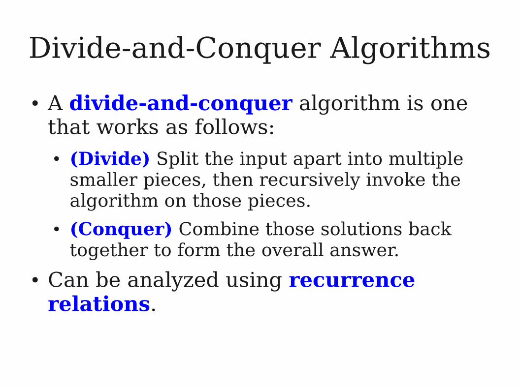
● A divide-and-conquer algorithm is one that works as follows:● (Divide) Split the input apart into multiple

smaller pieces, then recursively invoke the algorithm on those pieces.

● (Conquer) Combine those solutions back together to form the overall answer.

● Can be analyzed using recurrence relations.

Two Important Recurrences

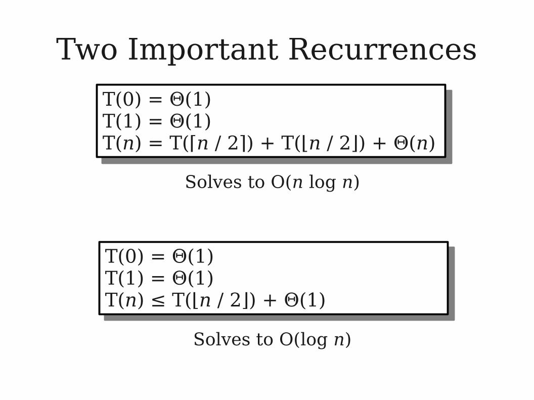
T(0) = Θ(1)T(1) = Θ(1)T(n) = T(⌈n / 2⌉) + T(⌊n / 2⌋) + Θ(n)

T(0) = Θ(1)T(1) = Θ(1)T(n) = T(⌈n / 2⌉) + T(⌊n / 2⌋) + Θ(n)

T(0) = Θ(1)T(1) = Θ(1)T(n) ≤ T(⌊n / 2⌋) + Θ(1)

T(0) = Θ(1)T(1) = Θ(1)T(n) ≤ T(⌊n / 2⌋) + Θ(1)

Solves to O(n log n)

Solves to O(log n)

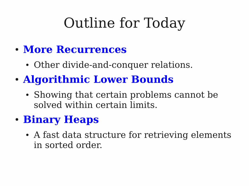
Outline for Today

● More Recurrences● Other divide-and-conquer relations.

● Algorithmic Lower Bounds● Showing that certain problems cannot be

solved within certain limits.

● Binary Heaps● A fast data structure for retrieving elements

in sorted order.

Another Algorithm:Maximizing Unimodal Arrays

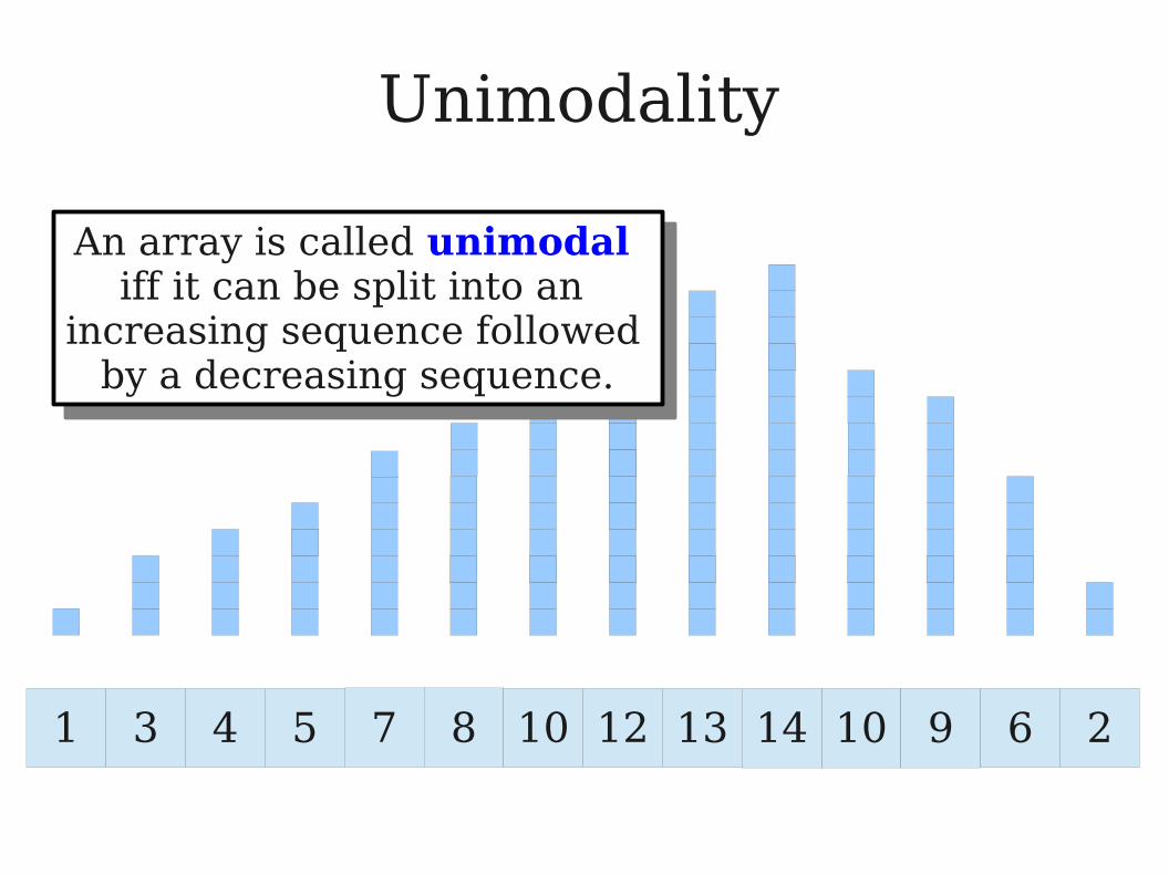
Unimodality

1 3 4 5 7 8 10 12 10 9 6 213 14

An array is called unimodal iff it can be split into an

increasing sequence followed by a decreasing sequence.

An array is called unimodal iff it can be split into an

increasing sequence followed by a decreasing sequence.

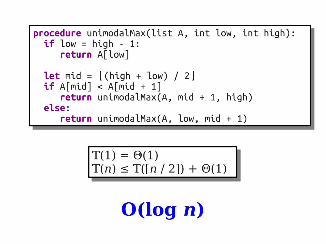
procedure unimodalMax(list A, int low, int high): if low = high - 1: return A[low]

let mid = (high + low) / 2⌊ ⌋ if A[mid] < A[mid + 1] return unimodalMax(A, mid + 1, high) else: return unimodalMax(A, low, mid + 1)

procedure unimodalMax(list A, int low, int high): if low = high - 1: return A[low]

let mid = (high + low) / 2⌊ ⌋ if A[mid] < A[mid + 1] return unimodalMax(A, mid + 1, high) else: return unimodalMax(A, low, mid + 1)

T(1) = Θ(1)T(n) ≤ T(⌈n / 2⌉) + Θ(1)

T(1) = Θ(1)T(n) ≤ T(⌈n / 2⌉) + Θ(1)

O(log n)

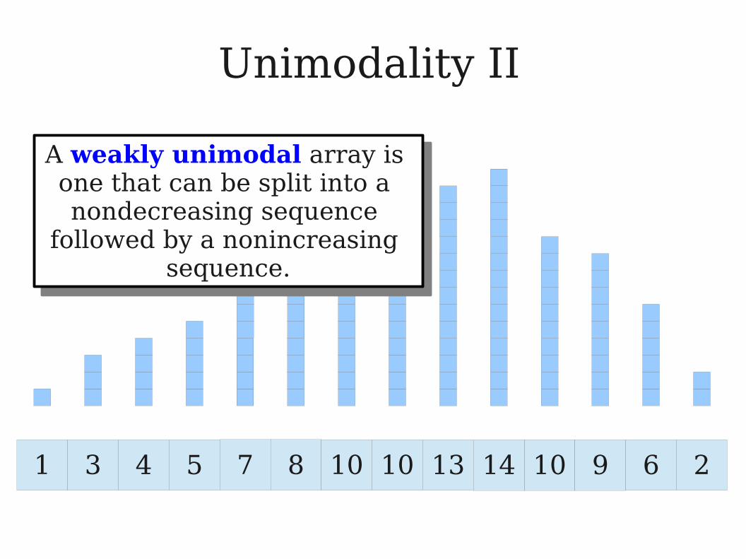
Unimodality II

1 3 4 5 7 8 10 10 10 9 6 213 14

A weakly unimodal array is one that can be split into a nondecreasing sequence

followed by a nonincreasing sequence.

A weakly unimodal array is one that can be split into a nondecreasing sequence

followed by a nonincreasing sequence.

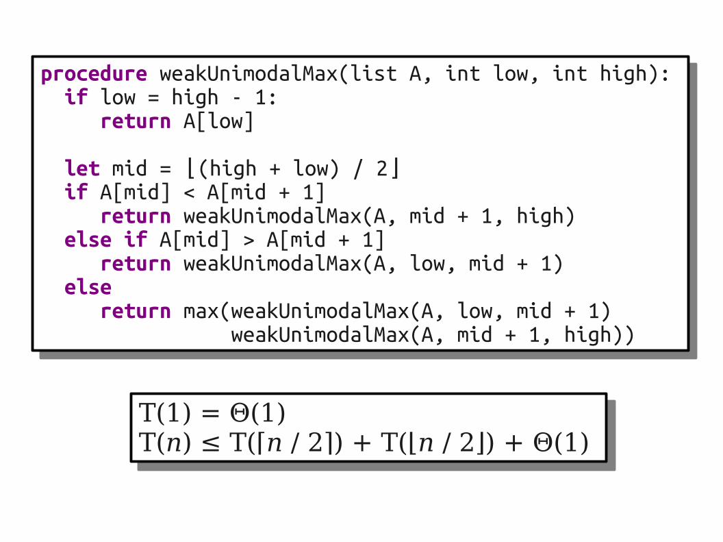
T(1) = Θ(1)T(n) ≤ T(⌈n / 2⌉) + T(⌊n / 2⌋) + Θ(1)

T(1) = Θ(1)T(n) ≤ T(⌈n / 2⌉) + T(⌊n / 2⌋) + Θ(1)

procedure weakUnimodalMax(list A, int low, int high): if low = high - 1: return A[low]

let mid = (high + low) / 2⌊ ⌋ if A[mid] < A[mid + 1] return weakUnimodalMax(A, mid + 1, high) else if A[mid] > A[mid + 1] return weakUnimodalMax(A, low, mid + 1) else return max(weakUnimodalMax(A, low, mid + 1) weakUnimodalMax(A, mid + 1, high))

procedure weakUnimodalMax(list A, int low, int high): if low = high - 1: return A[low]

let mid = (high + low) / 2⌊ ⌋ if A[mid] < A[mid + 1] return weakUnimodalMax(A, mid + 1, high) else if A[mid] > A[mid + 1] return weakUnimodalMax(A, low, mid + 1) else return max(weakUnimodalMax(A, low, mid + 1) weakUnimodalMax(A, mid + 1, high))

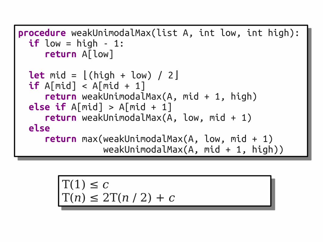
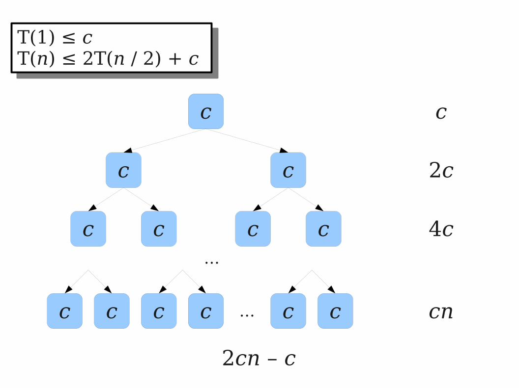
T(1) ≤ cT(n) ≤ 2T(n / 2) + c

T(1) ≤ cT(n) ≤ 2T(n / 2) + c

procedure weakUnimodalMax(list A, int low, int high): if low = high - 1: return A[low]

let mid = (high + low) / 2⌊ ⌋ if A[mid] < A[mid + 1] return weakUnimodalMax(A, mid + 1, high) else if A[mid] > A[mid + 1] return weakUnimodalMax(A, low, mid + 1) else return max(weakUnimodalMax(A, low, mid + 1) weakUnimodalMax(A, mid + 1, high))

procedure weakUnimodalMax(list A, int low, int high): if low = high - 1: return A[low]

let mid = (high + low) / 2⌊ ⌋ if A[mid] < A[mid + 1] return weakUnimodalMax(A, mid + 1, high) else if A[mid] > A[mid + 1] return weakUnimodalMax(A, low, mid + 1) else return max(weakUnimodalMax(A, low, mid + 1) weakUnimodalMax(A, mid + 1, high))

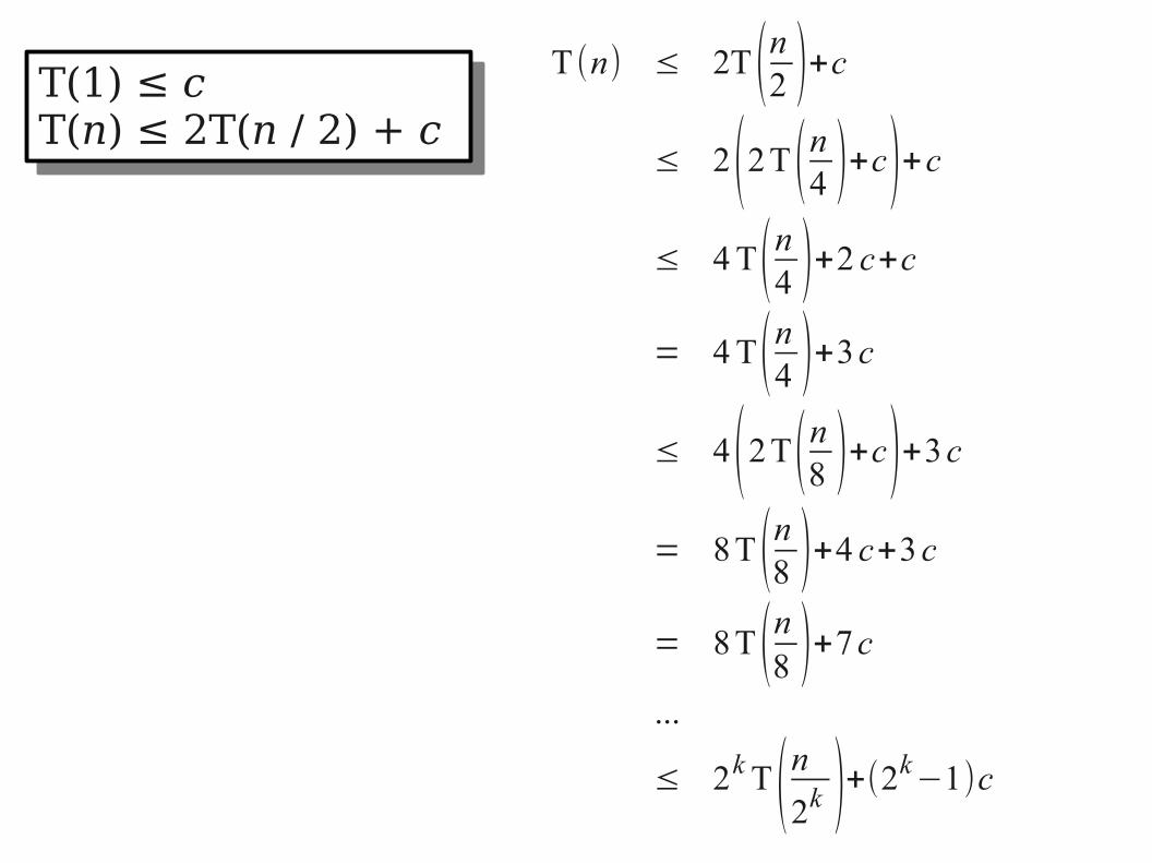
T (n) ≤ 2T (n2 )+c≤ 2(2T (n4 )+c)+c≤ 4 T(n4 )+2 c+c

= 4 T(n4 )+3c

≤ 4(2T(n8 )+c)+3c

= 8 T (n8 )+4 c+3c

= 8 T (n8 )+7c

...

≤ 2kT (n2k )+(2k−1)c

T(1) ≤ cT(n) ≤ 2T(n / 2) + c

T(1) ≤ cT(n) ≤ 2T(n / 2) + c

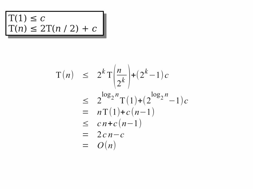
T (n) ≤ 2k T(n2k )+(2k−1)c

≤ 2log2 nT (1)+(2

log2 n−1)c= nT (1)+c (n−1)

≤ c n+c (n−1)

= 2c n−c= O (n)

T(1) ≤ cT(n) ≤ 2T(n / 2) + c

T(1) ≤ cT(n) ≤ 2T(n / 2) + c

T(1) ≤ cT(n) ≤ 2T(n / 2) + c

T(1) ≤ cT(n) ≤ 2T(n / 2) + c

c

c c

c c c c

c c c c c c

…

…

c

2c

4c

cn

2cn – c

Another Recurrence Relation

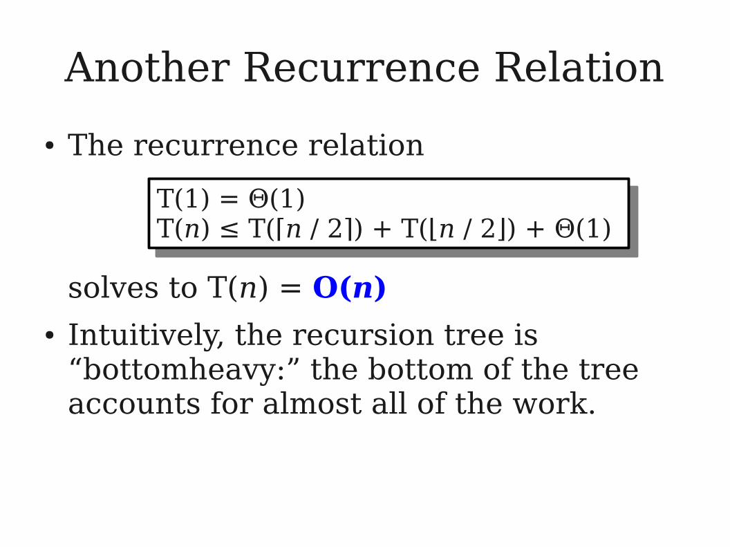
● The recurrence relation

solves to T(n) = O(n)● Intuitively, the recursion tree is

“bottomheavy:” the bottom of the tree accounts for almost all of the work.

T(1) = Θ(1)T(n) ≤ T(⌈n / 2⌉) + T(⌊n / 2⌋) + Θ(1)

T(1) = Θ(1)T(n) ≤ T(⌈n / 2⌉) + T(⌊n / 2⌋) + Θ(1)

Unimodal Arrays

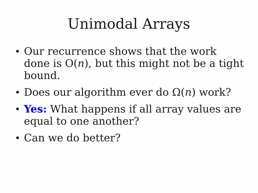
● Our recurrence shows that the work done is O(n), but this might not be a tight bound.

● Does our algorithm ever do Ω(n) work?● Yes: What happens if all array values are

equal to one another?● Can we do better?

A Lower Bound

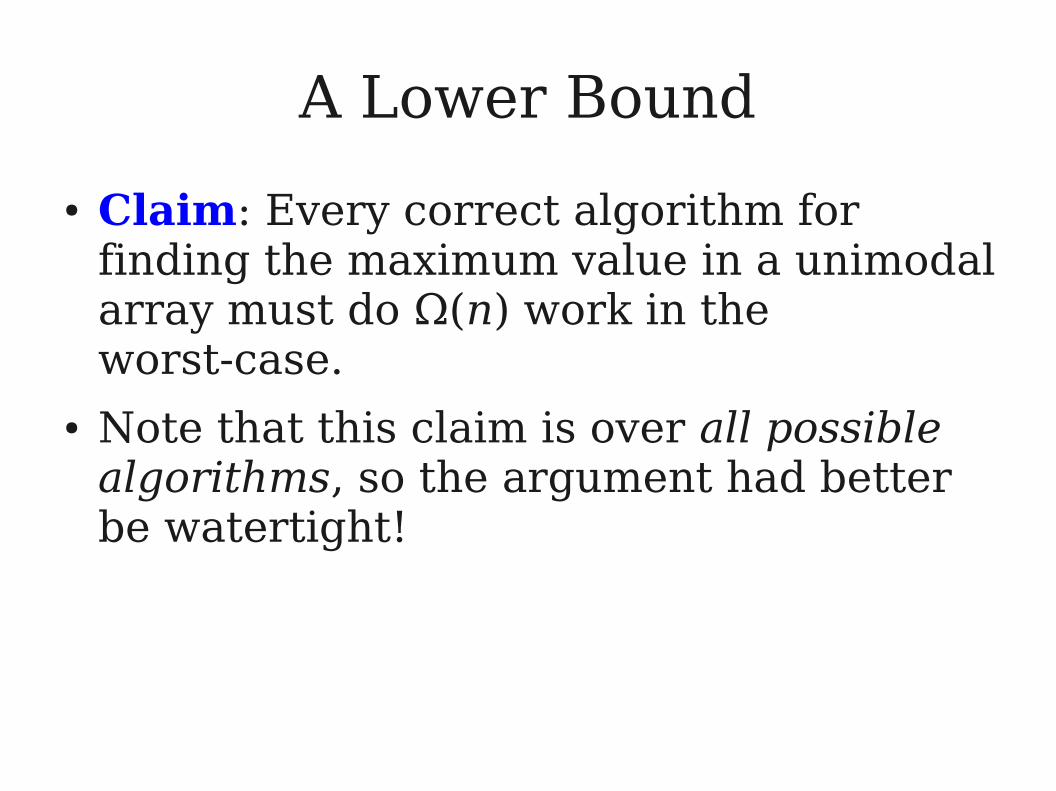
● Claim: Every correct algorithm for finding the maximum value in a unimodal array must do Ω(n) work in the worst-case.

● Note that this claim is over all possible algorithms, so the argument had better be watertight!

A Lower Bound

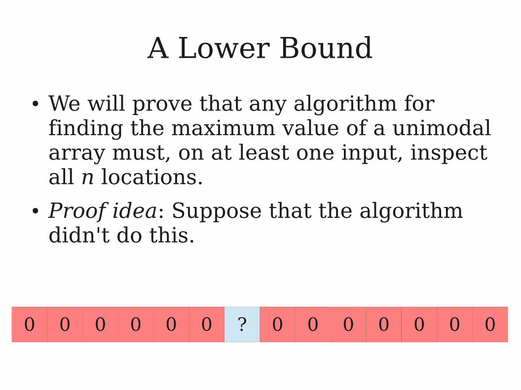
● We will prove that any algorithm for finding the maximum value of a unimodal array must, on at least one input, inspect all n locations.

● Proof idea: Suppose that the algorithm didn't do this.

0 0 0 0 0 0 ? 0 0 0 0 00 0

A Lower Bound

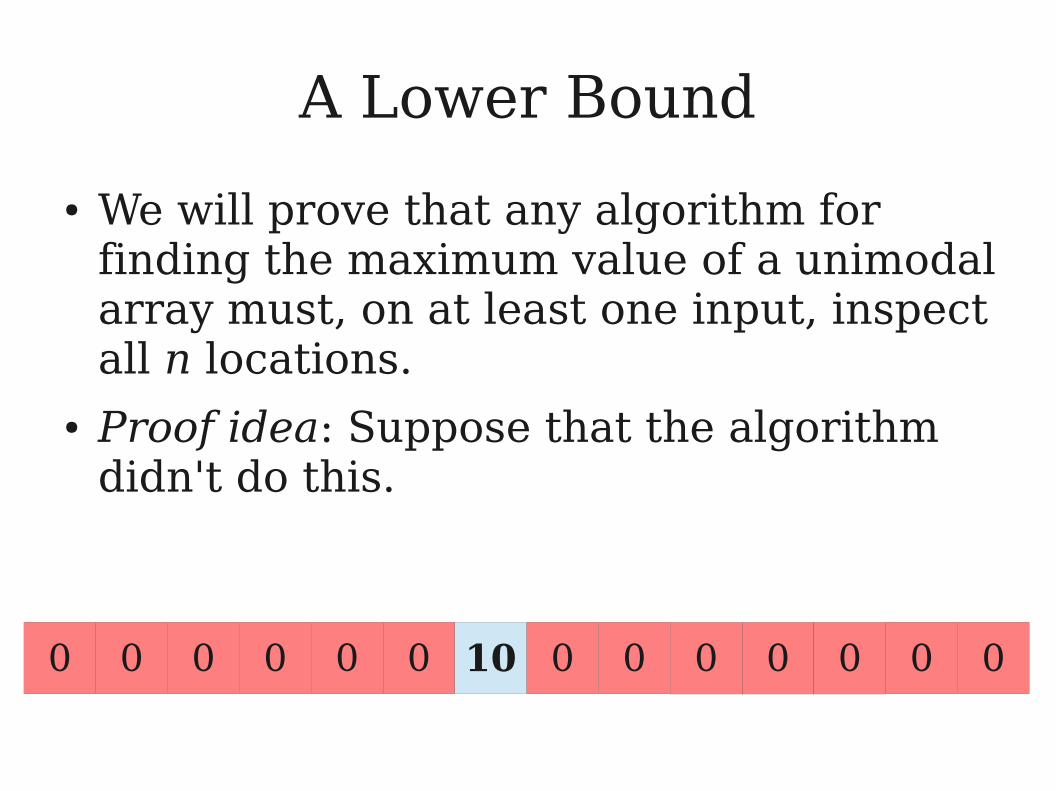
● We will prove that any algorithm for finding the maximum value of a unimodal array must, on at least one input, inspect all n locations.

● Proof idea: Suppose that the algorithm didn't do this.

0 0 0 0 0 0 10 0 0 0 0 00 0

A Lower Bound

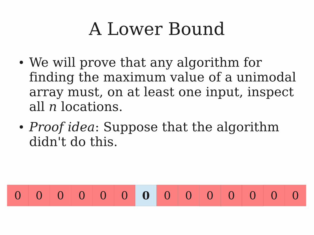
● We will prove that any algorithm for finding the maximum value of a unimodal array must, on at least one input, inspect all n locations.

● Proof idea: Suppose that the algorithm didn't do this.

0 0 0 0 0 0 0 0 0 0 0 00 0

Algorithmic Lower Bounds

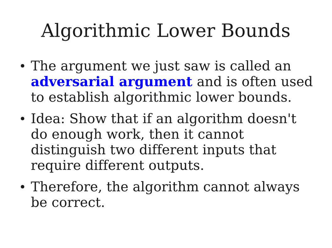
● The argument we just saw is called an adversarial argument and is often used to establish algorithmic lower bounds.

● Idea: Show that if an algorithm doesn't do enough work, then it cannot distinguish two different inputs that require different outputs.

● Therefore, the algorithm cannot always be correct.

o Notation

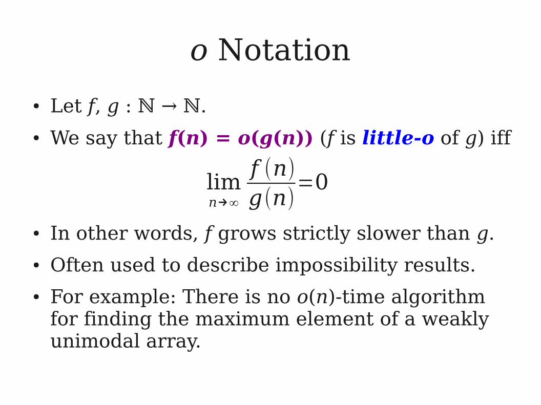
● Let f, g : ℕ → ℕ.

● We say that f(n) = o(g(n)) (f is little-o of g) iff

● In other words, f grows strictly slower than g.

● Often used to describe impossibility results.● For example: There is no o(n)-time algorithm

for finding the maximum element of a weakly unimodal array.

limn→∞

f (n)

g(n)=0

What Does This Mean?

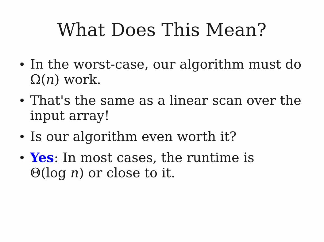
● In the worst-case, our algorithm must do Ω(n) work.

● That's the same as a linear scan over the input array!

● Is our algorithm even worth it?● Yes: In most cases, the runtime is

Θ(log n) or close to it.

Binary Heaps

Data Structures Matter

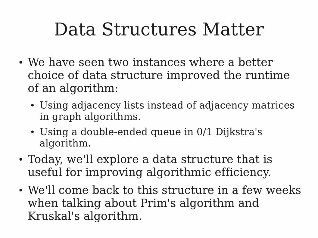
● We have seen two instances where a better choice of data structure improved the runtime of an algorithm:● Using adjacency lists instead of adjacency matrices

in graph algorithms.● Using a double-ended queue in 0/1 Dijkstra's

algorithm.

● Today, we'll explore a data structure that is useful for improving algorithmic efficiency.

● We'll come back to this structure in a few weeks when talking about Prim's algorithm and Kruskal's algorithm.

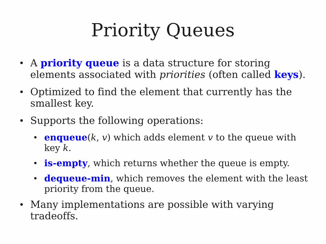
Priority Queues

● A priority queue is a data structure for storing elements associated with priorities (often called keys).

● Optimized to find the element that currently has the smallest key.

● Supports the following operations:

● enqueue(k, v) which adds element v to the queue with key k.

● is-empty, which returns whether the queue is empty.

● dequeue-min, which removes the element with the least priority from the queue.

● Many implementations are possible with varying tradeoffs.

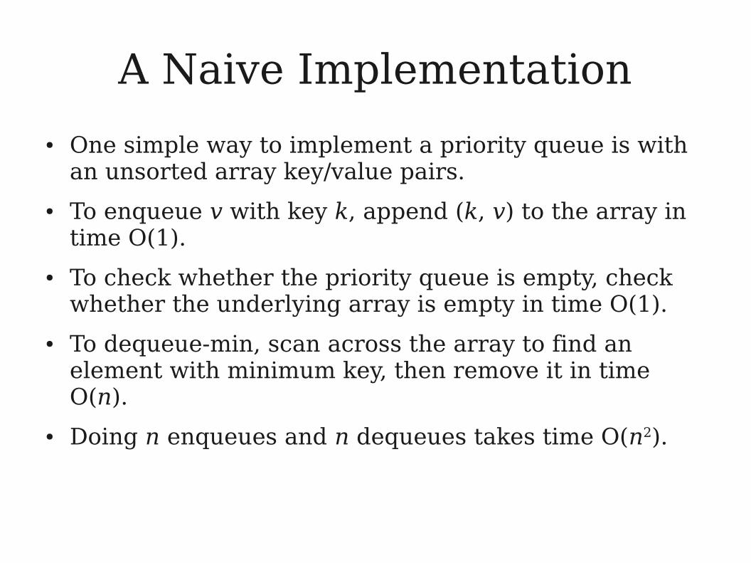
A Naive Implementation

● One simple way to implement a priority queue is with an unsorted array key/value pairs.

● To enqueue v with key k, append (k, v) to the array in time O(1).

● To check whether the priority queue is empty, check whether the underlying array is empty in time O(1).

● To dequeue-min, scan across the array to find an element with minimum key, then remove it in time O(n).

● Doing n enqueues and n dequeues takes time O(n2).

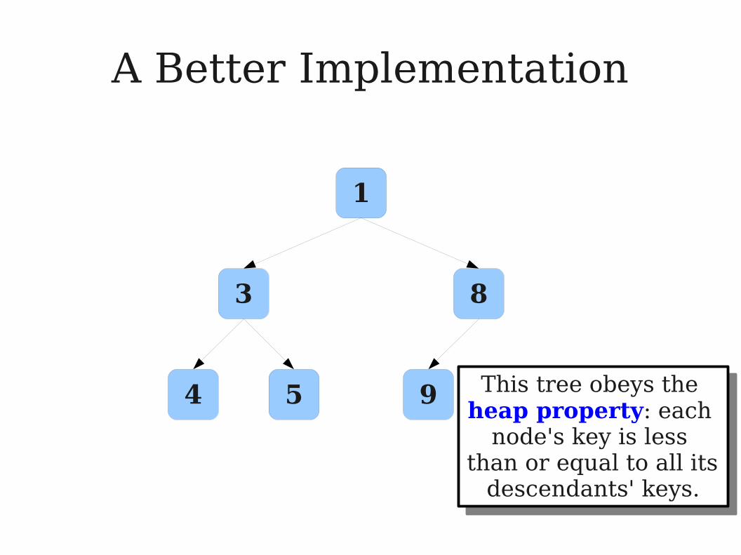
A Better Implementation

1

3 8

4 5 9 This tree obeys the heap property: each

node's key is less than or equal to all its

descendants' keys.

This tree obeys the heap property: each

node's key is less than or equal to all its

descendants' keys.

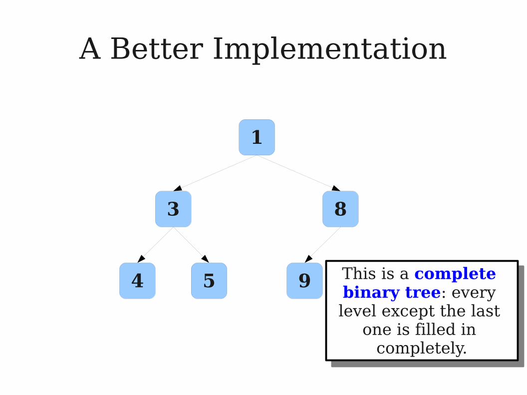
A Better Implementation

1

3 8

4 5 9 This is a complete binary tree: every level except the last

one is filled in completely.

This is a complete binary tree: every level except the last

one is filled in completely.

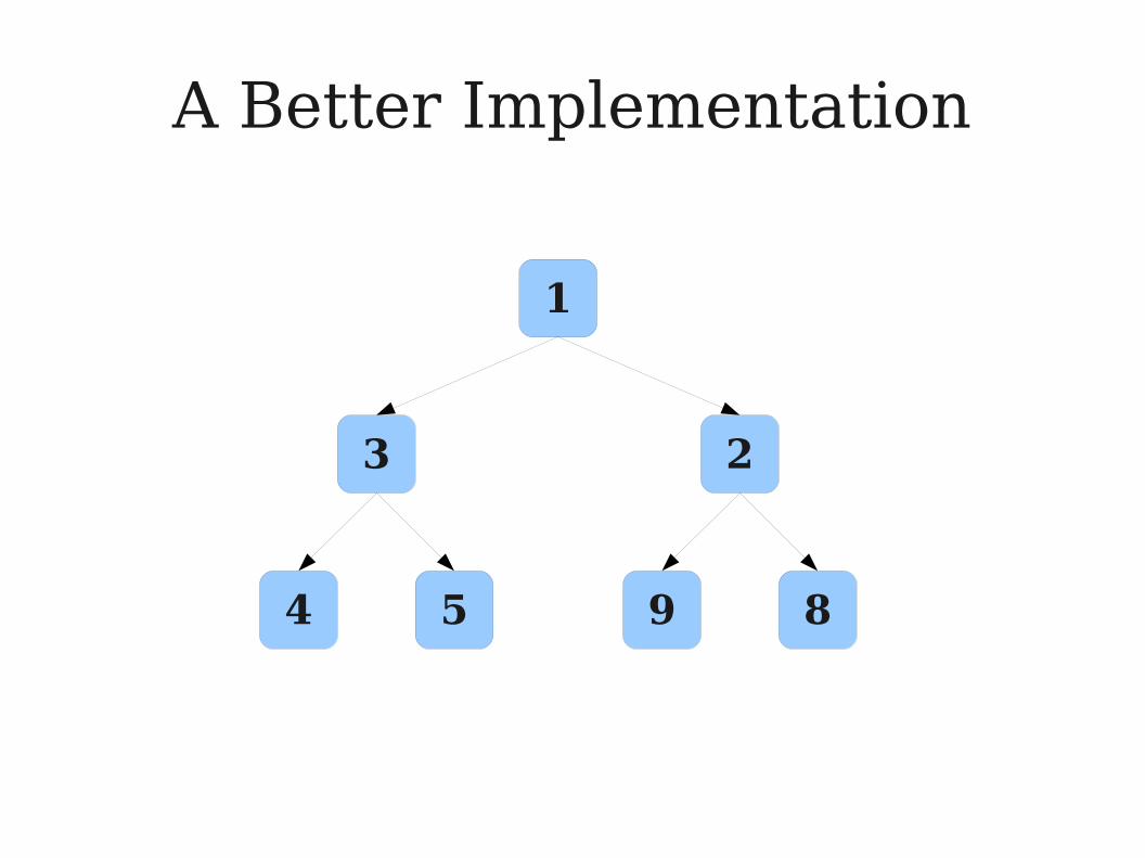
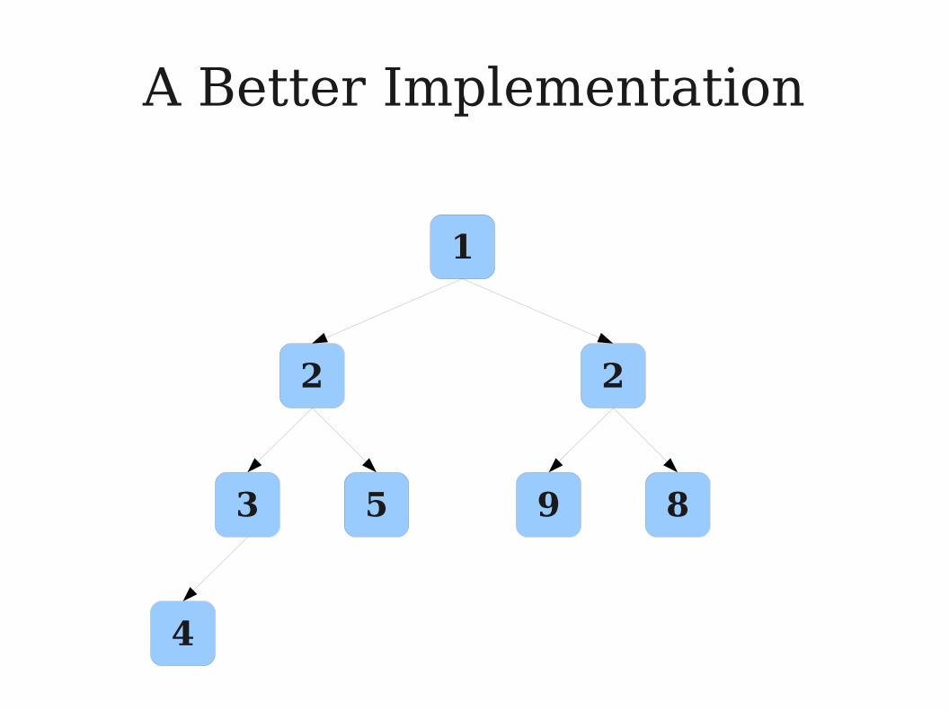
A Better Implementation

1

3 2

4 5 9 8

A Better Implementation

0

1 2

3 5 9 8

4

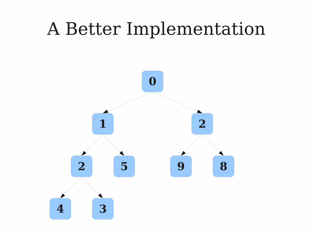
A Better Implementation

0

1 2

2 5 9 8

4 3

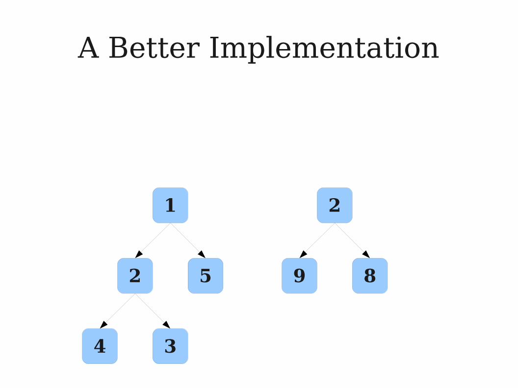
A Better Implementation

1 2

2 5 9 8

4 3

A Better Implementation

1 2

2 5 9 8

4

3

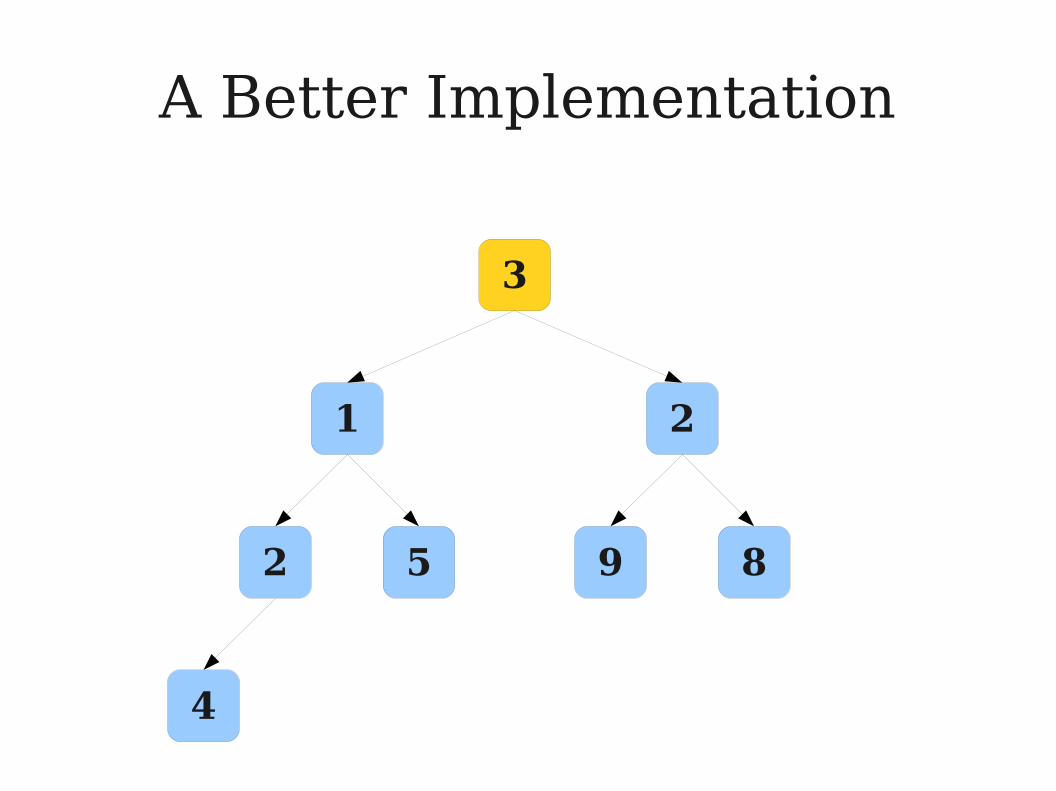
A Better Implementation

2 2

3 5 9 8

4

1

Binary Heap Efficiency

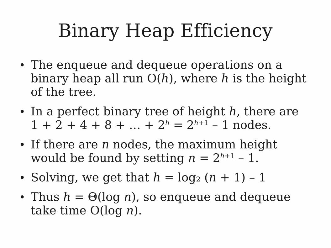
● The enqueue and dequeue operations on a binary heap all run O(h), where h is the height of the tree.

● In a perfect binary tree of height h, there are 1 + 2 + 4 + 8 + … + 2h = 2h+1 – 1 nodes.

● If there are n nodes, the maximum height would be found by setting n = 2h+1 – 1.

● Solving, we get that h = log₂ (n + 1) – 1

● Thus h = Θ(log n), so enqueue and dequeue take time O(log n).

Implementing Binary Heaps

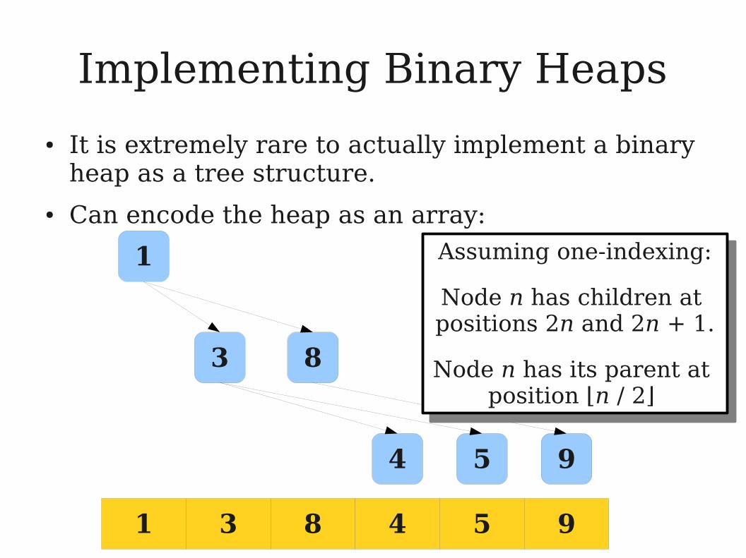
● It is extremely rare to actually implement a binary heap as a tree structure.

● Can encode the heap as an array:

1

3 8

4 5 9

1 3 8 4 5 9

Assuming one-indexing:

Node n has children at positions 2n and 2n + 1.

Node n has its parent at position ⌊n / 2⌋

Assuming one-indexing:

Node n has children at positions 2n and 2n + 1.

Node n has its parent at position ⌊n / 2⌋

Application: Heapsort

Heapsort

● The heapsort algorithm is as follows:● Build a max-heap from the array elements,

using the array itself to represent the heap.● Repeatedly dequeue from the heap until all

elements are placed in sorted order.

● This algorithm runs in time O(n log n), since it does n enqueues and n dequeues.

● Only requires O(1) auxiliary storage space, compared with O(n) space required in mergesort.

An Optimization: Heapify

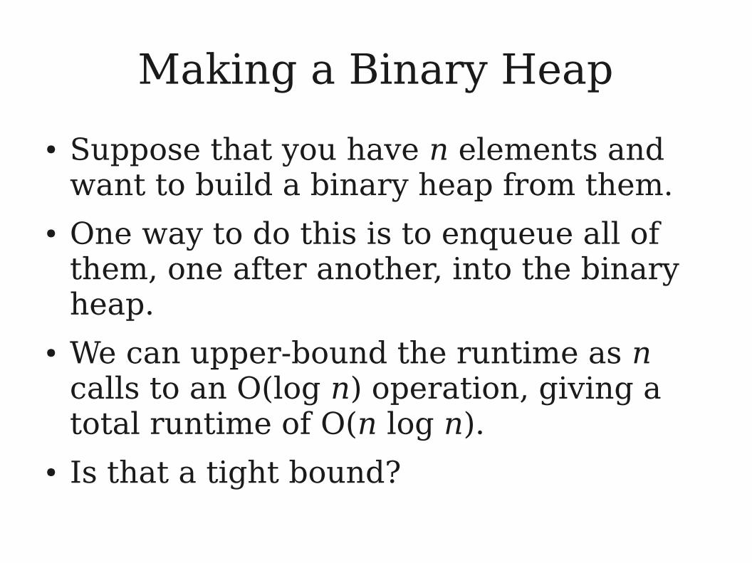
Making a Binary Heap

● Suppose that you have n elements and want to build a binary heap from them.

● One way to do this is to enqueue all of them, one after another, into the binary heap.

● We can upper-bound the runtime as n calls to an O(log n) operation, giving a total runtime of O(n log n).

● Is that a tight bound?

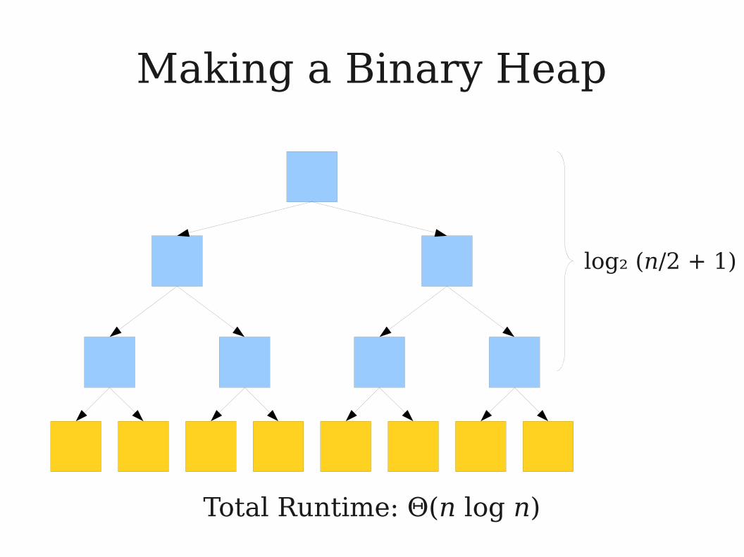
Making a Binary Heap

log₂ (n/2 + 1)

Total Runtime: Θ(n log n)

Quickly Making a Binary Heap

● Here is a slightly different algorithm for building a binary heap out of a set of data:● Put the nodes, in any order, into a complete

binary tree of the right size. (Shape property holds, but heap property might not.)

● For each node, starting at the bottom layer and going upward, run a bubble-down step on that node.

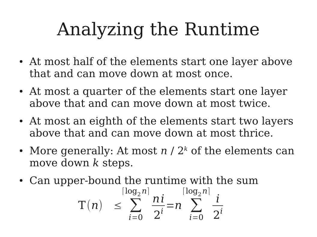
Analyzing the Runtime

● At most half of the elements start one layer above that and can move down at most once.

● At most a quarter of the elements start one layer above that and can move down at most twice.

● At most an eighth of the elements start two layers above that and can move down at most thrice.

● More generally: At most n / 2k of the elements can move down k steps.

● Can upper-bound the runtime with the sum

T (n) ≤ ∑i=0

⌈ log2n⌉ni

2i=n ∑

i=0

⌈ log2n⌉i

2i

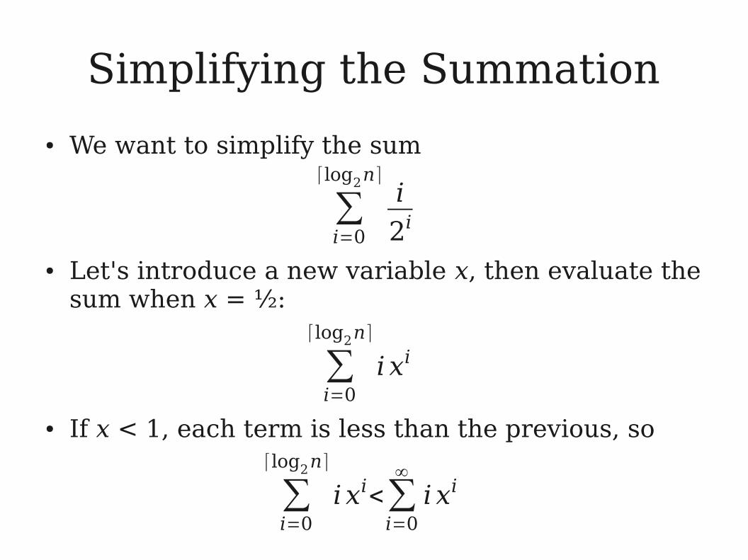
Simplifying the Summation

● We want to simplify the sum

● Let's introduce a new variable x, then evaluate the sum when x = ½:

● If x < 1, each term is less than the previous, so

∑i=0

⌈ log2n⌉i

2i

∑i=0

⌈ log2n⌉

i xi

∑i=0

⌈ log2n⌉

i xi<∑i=0

∞

i xi

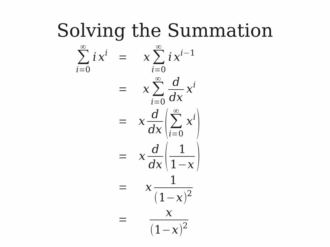
Solving the Summation∑i=0

∞

i xi = x∑i=0

∞

i xi−1

= x∑i=0

∞ ddx

xi

= xddx (∑i=0

∞

xi)= x

ddx ( 1

1−x )= x

1

(1−x)2

=x

(1−x)2

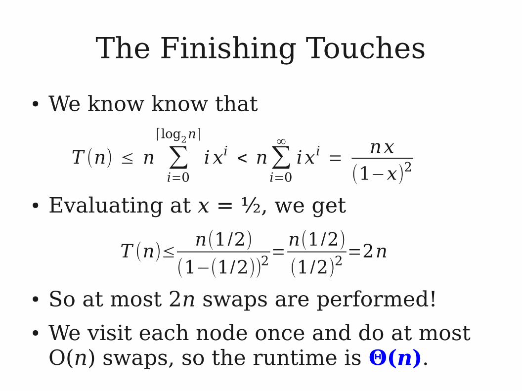
The Finishing Touches

● We know know that

● Evaluating at x = ½, we get

● So at most 2n swaps are performed!● We visit each node once and do at most

O(n) swaps, so the runtime is Θ(n).

T (n) ≤ n ∑i=0

⌈ log2n ⌉

i xi < n∑i=0

∞

i xi =nx

(1−x)2

T (n)≤n(1 /2)

(1−(1/2))2=

n(1 /2)

(1 /2)2=2n