Embed Size (px)
Citation preview

PART IIIGlobal Value Chains


Snapshot
• The coronavirus disease 2019 (COVID-19) pandemic has sharpened debates over the costs and benefits of global value chains (GVCs).
• Asia and the Pacific continues to feature some of the most integrated economies in the world, including Singapore; Taipei,China; and Viet Nam. In 2020, some 39% of the region’s exports involved indirect trading.
• Examining pandemic-induced demand shocks under varying hypothetical states of openness point to the amplifying effect of GVCs, as well as to the diverse experience of economies.
• Participation in GVCs and the size of the pandemic-related shock to gross domestic product (GDP) appear to have a U-shaped relationship. Greater participation is associated with a larger negative shock in 2020, but the relationship reverses beyond a certain point.
The COVID-19 Shock and the Two Faces of Global Value Chains
While debates over the risks of extended supply chains predate the COVID-19 pandemic, the unprecedented disruptions the coronavirus caused have escalated calls for some reshoring of economic activities and for greater economic self-sufficiency. What insights can a statistical analysis of the relationship between participation in GVCs and the economic impact from COVID-19 provide? Are economies that are more extensively embedded in international production networks more negatively affected by the pandemic, or less negatively affected?
In 2021, Key Indicators for Asia and the Pacific (Key Indicators) investigates this relationship between GVCs and economic performance during the pandemic. Using counterfactual exercises, it finds a wide range of outcomes for economies. However, on average, GVCs slightly amplified the effect of shocks via exposure to depressed foreign demand, compared to the counterfactual scenarios of autarky and bilateral-only trade. In a cross-economy analysis, it also finds a U-shaped relationship between GVC participation and the COVID-19 shock to growth, indicating again the heterogeneity of outcomes among economies. GVCs clearly have the power to both mitigate and amplify global disruptions.

230 Key Indicators for Asia and the Pacific 2021
The two faces of global value chains. The pandemic has highlighted the capacity for complex production-sharing arrangements to both mitigate and amplify shocks.
In a continuing effort to sharpen analytical tools, this edition of Key Indicators also revisits the GVC framework the publication first presented in 2015, updating and streamlining it in a new exposition that can be found in Appendix 3.1. The analyses and tables in Part III all follow this revised framework. Because calculation of the indicators relies on the Asian Development Bank’s Multiregional Input–Output (MRIO) Database, only 26 of the bank’s 49 member economies from Asia and the Pacific can be included: 24 developing economies, plus Australia and Japan.1
The COVID-19 Shock Under Different Trading Scenarios
Shocks such as the COVID-19 pandemic highlight the trade-offs that come with global economic integration. While an economy that is highly reliant on foreign markets is dependent on other economies whose performance has been hit hard by lockdowns, diversification can provide a buffer against plunges in domestic demand.
Quantifying this trade-off can be done through a counterfactual exercise that models COVID-19 demand shocks through prevailing input-output structures under three scenarios: autarky, classical trading, and GVCs. Depending on the scenario, an economy’s GDP is modeled to respond only to certain sources of demand. The first scenario of
1 The data presented in Part III are not official statistics. Production and trade data from various sources were integrated into the input–output economic framework and adjusted to conform with specific macroeconomic concepts. As such, data and statistics presented here could differ from relevant official statistics.
Global Value Chains
231Global Value Chains
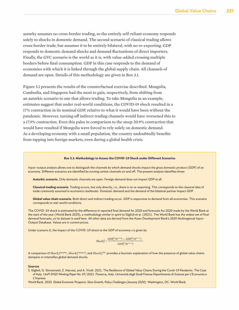
autarky assumes no cross-border trading, so the entirely self-reliant economy responds solely to shocks in domestic demand. The second scenario of classical trading allows cross-border trade, but assumes it to be entirely bilateral, with no re-exporting. GDP responds to domestic demand shocks and demand fluctuations of direct importers. Finally, the GVC scenario is the world as it is, with value-added crossing multiple borders before final consumption. GDP in this case responds to the demand of economies with which it is linked through the global supply chain. All channels of demand are open. Details of this methodology are given in Box 3.1.
Figure 3.1 presents the results of the counterfactual exercise described. Mongolia, Cambodia, and Singapore had the most to gain, respectively, from shifting from an autarkic scenario to one that allows trading. To take Mongolia as an example, estimates suggest that under real-world conditions, the COVID-19 shock resulted in a 17% contraction in its nominal GDP, relative to what it would have been without the pandemic. However, turning off indirect trading channels would have worsened this to a 17.9% contraction. Even this pales in comparison to the steep 20.9% contraction that would have resulted if Mongolia were forced to rely solely on domestic demand. As a developing economy with a small population, the country undoubtedly benefits from tapping into foreign markets, even during a global health crisis.
Box 3.1: Methodology to Assess the COVID-19 Shock under Different Scenarios
Input–output analysis allows one to distinguish the channels by which demand shocks impact the gross domestic product (GDP) of an economy. Different scenarios are identified by turning certain channels on and off. The present analysis identifies three:
Autarkic scenario. Only domestic channels are open. Foreign demand does not impact GDP at all.
Classical trading scenario. Trading occurs, but only directly, i.e., there is no re-exporting. This corresponds to the classical idea of trade commonly assumed in economics textbooks. Domestic demand and the demand of the bilateral partner impact GDP.
Global value chain scenario. Both direct and indirect trading occur. GDP is responsive to demand from all economies. This scenario corresponds to real-world conditions.
The COVID-19 shock is estimated by the difference in reported final demand for 2020 and forecasts for 2020 made by the World Bank at the start of the year (World Bank 2020), a methodology similar in spirit to Giglioli et al. (2021). The World Bank has the widest set of final demand forecasts, so its dataset is used here. All other data are derived from the Asian Development Bank’s 2020 Multiregional Input–Output Database. Values are in current prices.
Under scenario R, the impact of the COVID-19 shock to the GDP of economy s is given by
ShocksR GDPs
R (Yactual) — GDPsR (Yforecast)
GDPsR (Yforecast)
=
A comparison of ShocksAutarky, Shocks
Classical, and ShocksGVC provides a heuristic explanation of how the presence of global value chains
dampens or intensifies global demand shocks.
SourcesS. Giglioli, G. Giovannetti, E. Marvasi, and A. Vivoli. 2021. The Resilience of Global Value Chains During the Covid-19 Pandemic: The Case
of Italy. UniFI DISEI Working Paper No. 07/2021. Florence, Italy: Università degli Studi Firenze Dipartimento di Scienze per L’Economia e L’Impresa.
World Bank. 2020. Global Economic Prospects: Slow Growth, Policy Challenges (January 2020). Washington, DC: World Bank.
232 Key Indicators for Asia and the Pacific 2021
On the other end is Fiji, a tourism-oriented economy. Under the GVC scenario, the COVID-19 shock contracted the country’s nominal GDP by 21.2% relative to a pandemic-free 2020, comparable to the 21.5% contraction under the classical trading scenario. However, excluding all external demand channels brings the contraction down to 13.3%. Fiji’s high exposure to foreign demand has clearly amplified the shock of COVID-19. Indeed, it is notable that the only other economy that experienced a worse shock was Maldives, another small, tourism-reliant island economy.
Figure 3.1: The COVID-19 Shock under Different Trading ScenariosPe
rcen
t di�
eren
ce fr
om fo
reca
st
0%
–10%
–20%
Autarky
Mongolia
Cambodia
Singapore
Brunei Darussa
lamIndia
Bhutan
Pakistan
Indonesia PRC
Viet Nam
MalaysiaNepal
Philippines
Average
Republic of Korea
Australia
Maldives
BangladeshJapan
Hong Kong, China
Sri Lanka
Thailand
Kazakhstan
Taipei,China
Kyrgyz Republic
Lao PDR Fiji
8
4
0
–4
Perc
enta
ge-p
oint
di�
eren
ce
Classical tradingGVC
Autarky vs. GVCClassical trading vs. GVC
GVC = global value chain, Lao PDR = Lao People’s Democratic Republic, PRC = People’s Republic of China.Note: Average is unweighted.Sources: Asian Development Bank estimates; and Asian Development Bank Multiregional Input–Output Database, 2021.
Click here for figure data

Global Value Chains
233Global Value Chains
On average, GVCs have tended to amplify rather than dampen the COVID-19 shock for the 26 economies studied, with the shock being 0.6 points smaller under autarky compared with a GVC world. Note, however, that the difference is relatively small when compared with the realized shock of –10.9%. The average may also be skewed by the overrepresentation of trade-oriented developing economies in the sample. Indeed, a more sophisticated exercise performed by the Organisation for Economic Co-operation and Development (OECD) using a computable general equilibrium trade model finds that, in the presence of shocks, a “localized” regime tends to feature lower levels of GDP and increased instability relative to an “interconnected” regime (OECD 2021).
Global Value Chain Participation and COVID-19 Outcomes
For a clearer idea of how integration correlates with COVID-19 outcomes, a measure for GVC participation is necessary. This is obtained by categorizing the value of gross exports into those that stem from direct trading and those that stem from indirect trading. The latter consists of re-exports, imported inputs, and the purely double-counted quantities that arise when value-added crosses the same border twice or more. Details for decomposing exports are given in Box 3.2 and Appendix 3.1.
Box 3.2: Methodology to Assess Relationship Between Global Value Chain Participation and the COVID-19 Shock
Gross exports mask several distinct quantities that each provide information on the exporting economy’s global value chain (GVC) engagement. Disentangling these is the purpose of a value-added trade accounting framework, discussed more thoroughly in Appendix 3.1. To summarize, gross exports may be divided into five main categories:
DAVAX. Domestic value-added (DVA) exported to, and directly absorbed by, the importer.
REX. DVA exported to and re-exported by the importer, to eventually be absorbed abroad.
REF. DVA exported to and re-exported by the importer, to eventually be absorbed back home.
FVA. Foreign value-added. Imported inputs of goods and services in the overall exports of an economy.
PDC. Pure double-counting. In a GVC, some goods or services may cross the same border on two or more occasions.
DAVAX is direct trading, where value-added solely from the exporter is sent to, and absorbed solely by, the importer. The rest involve multiple border crossings before final consumption. Such indirect trading is what is understood in this analysis as GVC participation. The share of indirect trading in gross exports is the trade-based GVC participation rate.
As in Box 3.1, the COVID-19 shock is the difference between forecasted and actual growth rates for 2020. This time, the variable of interest is gross domestic product. Forecasts are from the October 2019 edition of the International Monetary Fund’s World Economic Outlook (IMF 2019), while actual growth rates are from the IMF’s April 2021 edition (IMF 2021). The IMF has the most complete set of gross domestic product forecasts for the Asian Development Bank Multiregional Input-Output economies.
In correlating GVC participation rates and the COVID-19 shock, participation rates for 2019 are used since rates for 2020 would have adjusted in some way to the pandemic, muddling the direction of causality.
SourcesInternational Monetary Fund (IMF). 2019. World Economic Outlook: Global Manufacturing Downturn, Rising Trade Barriers. Washington, DC:
International Monetary Fund.IMF. 2021. World Economic Outlook: Managing Divergent Recoveries. Washington, DC: International Monetary Fund.
234 Key Indicators for Asia and the Pacific 2021
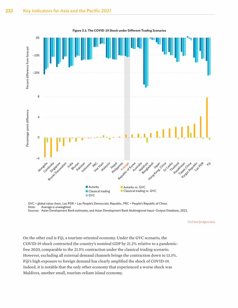
Looking at Asia and the Pacific’s exports in Figure 3.2 gives a notion of how integrated each economy is to GVCs. The green and red regions represent the import content of exports and thus gauge integration in a backward sense. The leaders here are the financial hub of Singapore and the manufacturing hubs of Viet Nam and Cambodia, all of whom had import contents of over 40%. These three take in substantial foreign value-added for processing, after which they pass this value-added along the chain. On the other end are economies such as Australia and Kazakhstan, whose commodity-rich exports naturally comprise mostly domestic content. Size is also a factor as large economies such as Indonesia, Japan, and the People’s Republic of China are able to source much of their inputs domestically.
Figure 3.2: Value-Added Categories in Asia and the Pacific’s Exports, 2020
SingaporeViet NamMalaysia
Taipei,ChinaCambodia
Republic of KoreaPhilippines
Brunei DarussalamThailand
KazakhstanKyrgyz Republic
MaldivesAverage
NepalMongolia
Hong Kong, ChinaIndonesia
JapanAustralia
IndiaPRC
Lao PDRFiji
BhutanSri Lanka
BangladeshPakistan
25% 50% 75%
Directly absorbedRe-exported and absorbed abroadRe-exported and returned home
Foreign value-addedPure double-counting
Lao PDR = Lao People’s Democratic Republic, PRC = People’s Republic of ChinaNote: Average is weighted by gross exports.Sources: Asian Development Bank estimates based on Koopman, Wang, and Wei (2014) and Borin and Mancini (2019); and Asian
Development Bank Multiregional Input–Output Database, 2021.
Click here for figure data
Global Value Chains
235Global Value Chains
Integration in the forward sense is measured by the medium and light blue regions, which represent how much of exports go on to be re-exported. The commodity-rich economies dominate this time, with Brunei Darussalam and Kazakhstan having over 25% of what they export passed further along the chain. The landlocked Lao People’s Democratic Republic also exhibited high forward integration, with re-exports occurring on 21% of its exports, possibly due to its reliance on ports in Viet Nam and Thailand for shipping its goods elsewhere. The fact that the backward-integrated economies of Cambodia and Viet Nam registered fairly low forward integration implies that they tend to serve final markets. A special type of forward integration, measured by the light blue regions, involves an economy’s exports eventually making their way back to its own domestic consumers. This suggests an economy that is positioned in the more upstream end of value chains. Of the economies sampled, only the People’s Republic of China had substantial exports of this kind.
The sum of backward and forward integration is equivalent to the share of indirect trading, what this analysis calls the GVC participation rate. The economies in Figure 3.2 are arranged in descending order of integration. The most integrated economies—Singapore; Viet Nam; Malaysia; Taipei,China; and Cambodia—are all in East Asia or Southeast Asia, and all registered GVC participation rates of 50% and above. The least integrated region was South Asia, with Bangladesh, Bhutan, India, Nepal, Pakistan, and Sri Lanka appearing in the bottom half of the chart. For Bangladesh and Pakistan in particular, over 75% of their trading was of the direct kind. Bucking the trend for the region is Maldives, whose substantial import content placed it among those with above-average integration.
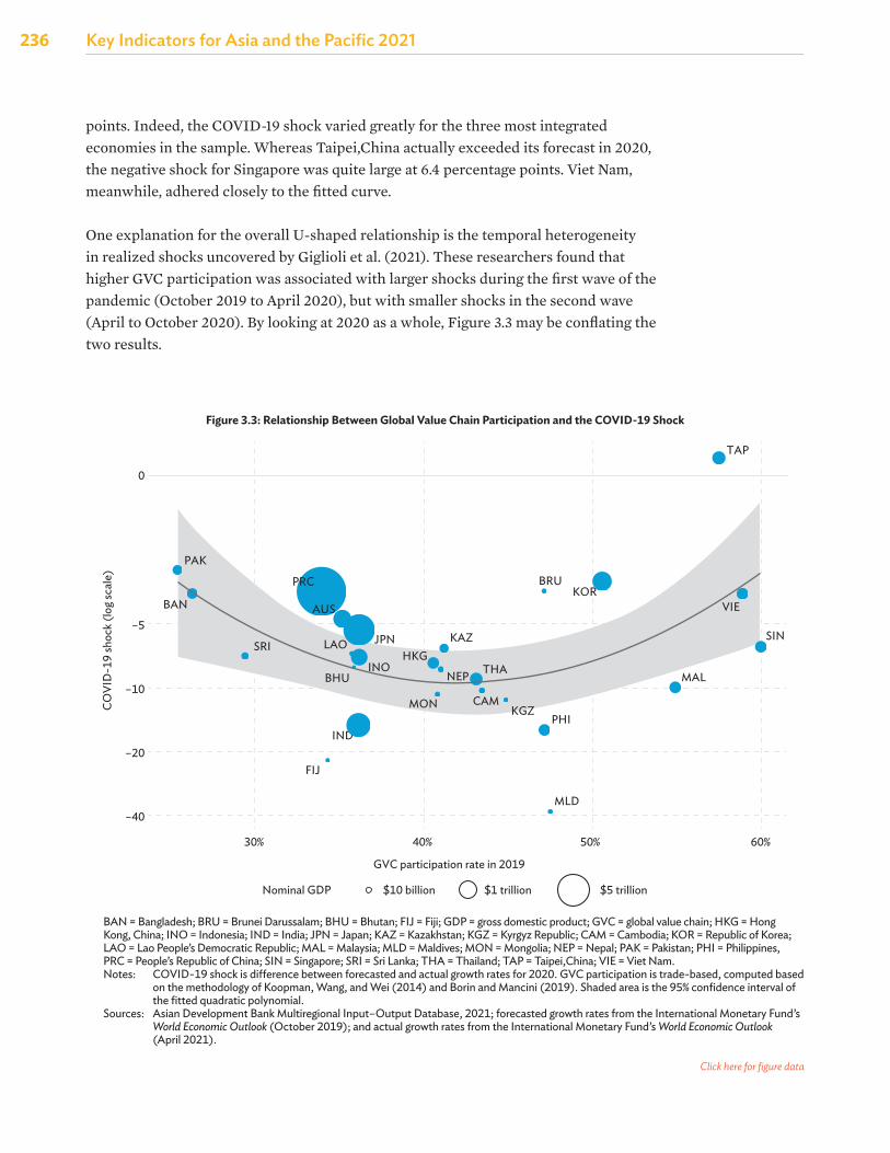
The variation in rates of GVC participation across these 26 economies provides an opportunity for examining how integration correlates with the size of the COVID-19 shock, again measured by the difference between forecasted and actual growth (Box 3.2). Results are plotted in Figure 3.3, which has GVC participation rates on the horizontal axis and the COVID-19 shock in log scale on the vertical axis. Point sizes reflect nominal GDP. A quadratic curve is fitted to reveal the estimated relationship, with the shaded band representing the 95% confidence interval.
Despite the limited sample size, a distinct U-shaped curve is detected between trade integration and the size of the COVID-19 shock. It appears that higher GVC participation is associated with larger negative shocks until a rate of about 45%, after which it becomes associated with smaller negative shocks. Contrast the experience of Pakistan, whose participation rate was 25% and whose 2020 growth was just 2.8 percentage points below the forecast, with that of Thailand, whose participation rate was 43% and whose growth was 9.1 points lower than the forecast. Then compare this with Viet Nam, whose participation rate was 59% and whose growth was just 3.6 points below the forecast.
It must be noted, however, that the estimated relationship has significant noise, especially at the highest rates of participation, largely because of the scarcity of data
236 Key Indicators for Asia and the Pacific 2021
points. Indeed, the COVID-19 shock varied greatly for the three most integrated economies in the sample. Whereas Taipei,China actually exceeded its forecast in 2020, the negative shock for Singapore was quite large at 6.4 percentage points. Viet Nam, meanwhile, adhered closely to the fitted curve.
One explanation for the overall U-shaped relationship is the temporal heterogeneity in realized shocks uncovered by Giglioli et al. (2021). These researchers found that higher GVC participation was associated with larger shocks during the first wave of the pandemic (October 2019 to April 2020), but with smaller shocks in the second wave (April to October 2020). By looking at 2020 as a whole, Figure 3.3 may be conflating the two results.
Figure 3.3: Relationship Between Global Value Chain Participation and the COVID-19 Shock
30%
FIJ
INDPHI
MAL
SIN
TAP
KORBRU
KAZ
THA
KGZCAMMON
NEP
HKGINO
BHU
SRI
BAN
PAK
LAO JPN
MLD
40%
GVC participation rate in 2019
Nominal GDP $10 billion $1 trillion $5 trillion
50% 60%
–5
0
–10
–20
–40
COVI
D-1
9 sh
ock
(log
scal
e)
VIE
PRC
AUS
BAN = Bangladesh; BRU = Brunei Darussalam; BHU = Bhutan; FIJ = Fiji; GDP = gross domestic product; GVC = global value chain; HKG = Hong Kong, China; INO = Indonesia; IND = India; JPN = Japan; KAZ = Kazakhstan; KGZ = Kyrgyz Republic; CAM = Cambodia; KOR = Republic of Korea; LAO = Lao People’s Democratic Republic; MAL = Malaysia; MLD = Maldives; MON = Mongolia; NEP = Nepal; PAK = Pakistan; PHI = Philippines, PRC = People’s Republic of China; SIN = Singapore; SRI = Sri Lanka; THA = Thailand; TAP = Taipei,China; VIE = Viet Nam.Notes: COVID-19 shock is difference between forecasted and actual growth rates for 2020. GVC participation is trade-based, computed based
on the methodology of Koopman, Wang, and Wei (2014) and Borin and Mancini (2019). Shaded area is the 95% confidence interval of the fitted quadratic polynomial.
Sources: Asian Development Bank Multiregional Input–Output Database, 2021; forecasted growth rates from the International Monetary Fund’s World Economic Outlook (October 2019); and actual growth rates from the International Monetary Fund’s World Economic Outlook (April 2021).
Click here for figure data
Global Value Chains
237Global Value Chains
On a final note, it must be emphasized that Figure 3.3 is specific to the COVID-19 pandemic and, given a different shock, these results may not necessarily hold. As such, no prescriptive conclusions regarding an “optimal” GVC participation rate should be taken from these outcomes.
Conclusion
The COVID-19 pandemic has revealed quite dramatically the two faces of GVCs. On the one hand, by connecting producers and consumers in long and complex supply chains, GVCs allow for the diversification of economic activity, and this can lower risk. On the other hand, a system-wide crisis like the 2020 pandemic turns these connections into channels for the amplification of shocks, thereby heightening risk. As the fates of economies become more entangled with one another, underperformance anywhere becomes a concern everywhere.
Nevertheless, just as success rates in managing the coronavirus stem largely from good policymaking, so too will the consequences of global integration. It is this that will ultimately determine which of the two faces of GVCs becomes ascendant for each economy in a post-pandemic world.
238 Key Indicators for Asia and the Pacific 2021
Appendix 3.1: An Analytical Framework for Studying Global Value Chains
Introduction
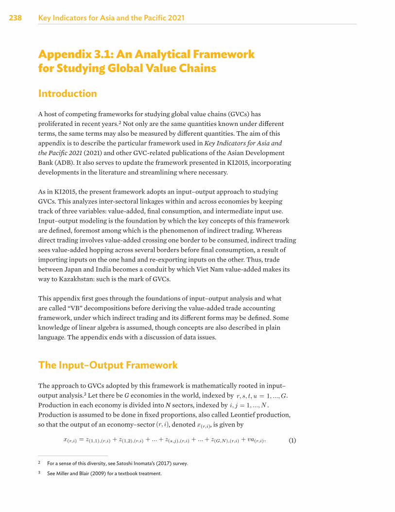
A host of competing frameworks for studying global value chains (GVCs) has proliferated in recent years.2 Not only are the same quantities known under different terms, the same terms may also be measured by different quantities. The aim of this appendix is to describe the particular framework used in Key Indicators for Asia and the Pacific 2021 (2021) and other GVC-related publications of the Asian Development Bank (ADB). It also serves to update the framework presented in KI2015, incorporating developments in the literature and streamlining where necessary.
As in KI2015, the present framework adopts an input–output approach to studying GVCs. This analyzes inter-sectoral linkages within and across economies by keeping track of three variables: value-added, final consumption, and intermediate input use. Input–output modeling is the foundation by which the key concepts of this framework are defined, foremost among which is the phenomenon of indirect trading. Whereas direct trading involves value-added crossing one border to be consumed, indirect trading sees value-added hopping across several borders before final consumption, a result of importing inputs on the one hand and re-exporting inputs on the other. Thus, trade between Japan and India becomes a conduit by which Viet Nam value-added makes its way to Kazakhstan: such is the mark of GVCs.
This appendix first goes through the foundations of input–output analysis and what are called “VB” decompositions before deriving the value-added trade accounting framework, under which indirect trading and its different forms may be defined. Some knowledge of linear algebra is assumed, though concepts are also described in plain language. The appendix ends with a discussion of data issues.
The Input–Output Framework
The approach to GVCs adopted by this framework is mathematically rooted in input–output analysis.3 Let there be G economies in the world, indexed by
Appendix 3.1: An Analytical Framework for Studying Global ValueChains
Introduction
A host of competing frameworks for studying global value chains (GVCs) has proliferated in recent years.1
Not only are the same quantities known under different terms, the same terms may also be measured bydifferent quantities. The aim of this appendix is to describe the particular framework used in Key Indicatorsfor Asia and the Pacific 2021 (2021) and other GVC-related publications of the Asian Development Bank(ADB). It also serves to update the framework presented in KI2015, incorporating developments in theliterature and streamlining where necessary.
As in KI2015, the present framework adopts an input–output approach to studying GVCs. This analyzesinter-sectoral linkages within and across economies by keeping track of three variables: value-added, finalconsumption, and intermediate input use. Input–output modeling is the foundation by which the keyconcepts of this framework are defined, foremost among which is the phenomenon of indirect trading.Whereas direct trading involves value-added crossing one border to be consumed, indirect trading seesvalue-added hopping across several borders before final consumption, a result of importing inputs on theone hand and re-exporting inputs on the other. Thus, trade between Japan and India becomes a conduit bywhich Viet Nam value-added makes its way to Kazakhstan: such is the mark of GVCs.
This appendix first goes through the foundations of input–output analysis and what are called “VB”decompositions before deriving the value-added trade accounting framework, under which indirect tradingand its different forms may be defined. Some knowledge of linear algebra is assumed, though concepts arealso described in plain language. The appendix ends with a discussion of data issues.
The Input–Output Framework
The approach to GVCs adopted by this framework is mathematically rooted in input–output analysis.2 Letthere be G economies in the world, indexed by r, s, t, u = 1, ..., G. Production in each economy is dividedinto N sectors, indexed by i, j = 1, ..., N . Production is assumed to be done in fixed proportions, also calledLeontief production, so that the output of an economy–sector (r, i), denoted x(r,i), is given by
x(r,i) = z(1,1),(r,i) + z(1,2),(r,i) + ... + z(s,j),(r,i) + ... + z(G,N),(r,i) + va(r,i), (1)1For a sense of this diversity, see Satoshi Inomata’s (2017) survey.2See Miller and Blair (2009) for a textbook treatment.
1
. Production in each economy is divided into N sectors, indexed by
Appendix 3.1: An Analytical Framework for Studying Global ValueChains
Introduction
A host of competing frameworks for studying global value chains (GVCs) has proliferated in recent years.1
Not only are the same quantities known under different terms, the same terms may also be measured bydifferent quantities. The aim of this appendix is to describe the particular framework used in Key Indicatorsfor Asia and the Pacific 2021 (2021) and other GVC-related publications of the Asian Development Bank(ADB). It also serves to update the framework presented in KI2015, incorporating developments in theliterature and streamlining where necessary.
As in KI2015, the present framework adopts an input–output approach to studying GVCs. This analyzesinter-sectoral linkages within and across economies by keeping track of three variables: value-added, finalconsumption, and intermediate input use. Input–output modeling is the foundation by which the keyconcepts of this framework are defined, foremost among which is the phenomenon of indirect trading.Whereas direct trading involves value-added crossing one border to be consumed, indirect trading seesvalue-added hopping across several borders before final consumption, a result of importing inputs on theone hand and re-exporting inputs on the other. Thus, trade between Japan and India becomes a conduit bywhich Viet Nam value-added makes its way to Kazakhstan: such is the mark of GVCs.
This appendix first goes through the foundations of input–output analysis and what are called “VB”decompositions before deriving the value-added trade accounting framework, under which indirect tradingand its different forms may be defined. Some knowledge of linear algebra is assumed, though concepts arealso described in plain language. The appendix ends with a discussion of data issues.
The Input–Output Framework
The approach to GVCs adopted by this framework is mathematically rooted in input–output analysis.2 Letthere be G economies in the world, indexed by r, s, t, u = 1, ..., G. Production in each economy is dividedinto N sectors, indexed by i, j = 1, ..., N . Production is assumed to be done in fixed proportions, also calledLeontief production, so that the output of an economy–sector (r, i), denoted x(r,i), is given by
x(r,i) = z(1,1),(r,i) + z(1,2),(r,i) + ... + z(s,j),(r,i) + ... + z(G,N),(r,i) + va(r,i), (1)1For a sense of this diversity, see Satoshi Inomata’s (2017) survey.2See Miller and Blair (2009) for a textbook treatment.
1
. Production is assumed to be done in fixed proportions, also called Leontief production, so that the output of an economy–sector
Appendix 3.1: An Analytical Framework for Studying Global ValueChains
Introduction
A host of competing frameworks for studying global value chains (GVCs) has proliferated in recent years.1
Not only are the same quantities known under different terms, the same terms may also be measured bydifferent quantities. The aim of this appendix is to describe the particular framework used in Key Indicatorsfor Asia and the Pacific 2021 (2021) and other GVC-related publications of the Asian Development Bank(ADB). It also serves to update the framework presented in KI2015, incorporating developments in theliterature and streamlining where necessary.
As in KI2015, the present framework adopts an input–output approach to studying GVCs. This analyzesinter-sectoral linkages within and across economies by keeping track of three variables: value-added, finalconsumption, and intermediate input use. Input–output modeling is the foundation by which the keyconcepts of this framework are defined, foremost among which is the phenomenon of indirect trading.Whereas direct trading involves value-added crossing one border to be consumed, indirect trading seesvalue-added hopping across several borders before final consumption, a result of importing inputs on theone hand and re-exporting inputs on the other. Thus, trade between Japan and India becomes a conduit bywhich Viet Nam value-added makes its way to Kazakhstan: such is the mark of GVCs.
This appendix first goes through the foundations of input–output analysis and what are called “VB”decompositions before deriving the value-added trade accounting framework, under which indirect tradingand its different forms may be defined. Some knowledge of linear algebra is assumed, though concepts arealso described in plain language. The appendix ends with a discussion of data issues.
The Input–Output Framework
The approach to GVCs adopted by this framework is mathematically rooted in input–output analysis.2 Letthere be G economies in the world, indexed by r, s, t, u = 1, ..., G. Production in each economy is dividedinto N sectors, indexed by i, j = 1, ..., N . Production is assumed to be done in fixed proportions, also calledLeontief production, so that the output of an economy–sector (r, i), denoted x(r,i), is given by
x(r,i) = z(1,1),(r,i) + z(1,2),(r,i) + ... + z(s,j),(r,i) + ... + z(G,N),(r,i) + va(r,i), (1)1For a sense of this diversity, see Satoshi Inomata’s (2017) survey.2See Miller and Blair (2009) for a textbook treatment.
1
, denoted
Appendix 3.1: An Analytical Framework for Studying Global ValueChains
Introduction
A host of competing frameworks for studying global value chains (GVCs) has proliferated in recent years.1
Not only are the same quantities known under different terms, the same terms may also be measured bydifferent quantities. The aim of this appendix is to describe the particular framework used in Key Indicatorsfor Asia and the Pacific 2021 (2021) and other GVC-related publications of the Asian Development Bank(ADB). It also serves to update the framework presented in KI2015, incorporating developments in theliterature and streamlining where necessary.
As in KI2015, the present framework adopts an input–output approach to studying GVCs. This analyzesinter-sectoral linkages within and across economies by keeping track of three variables: value-added, finalconsumption, and intermediate input use. Input–output modeling is the foundation by which the keyconcepts of this framework are defined, foremost among which is the phenomenon of indirect trading.Whereas direct trading involves value-added crossing one border to be consumed, indirect trading seesvalue-added hopping across several borders before final consumption, a result of importing inputs on theone hand and re-exporting inputs on the other. Thus, trade between Japan and India becomes a conduit bywhich Viet Nam value-added makes its way to Kazakhstan: such is the mark of GVCs.
This appendix first goes through the foundations of input–output analysis and what are called “VB”decompositions before deriving the value-added trade accounting framework, under which indirect tradingand its different forms may be defined. Some knowledge of linear algebra is assumed, though concepts arealso described in plain language. The appendix ends with a discussion of data issues.
The Input–Output Framework
The approach to GVCs adopted by this framework is mathematically rooted in input–output analysis.2 Letthere be G economies in the world, indexed by r, s, t, u = 1, ..., G. Production in each economy is dividedinto N sectors, indexed by i, j = 1, ..., N . Production is assumed to be done in fixed proportions, also calledLeontief production, so that the output of an economy–sector (r, i), denoted x(r,i), is given by
x(r,i) = z(1,1),(r,i) + z(1,2),(r,i) + ... + z(s,j),(r,i) + ... + z(G,N),(r,i) + va(r,i), (1)1For a sense of this diversity, see Satoshi Inomata’s (2017) survey.2See Miller and Blair (2009) for a textbook treatment.
1
, is given by
Appendix 3.1: An Analytical Framework for Studying Global ValueChains
Introduction
A host of competing frameworks for studying global value chains (GVCs) has proliferated in recent years.1
Not only are the same quantities known under different terms, the same terms may also be measured bydifferent quantities. The aim of this appendix is to describe the particular framework used in Key Indicatorsfor Asia and the Pacific 2021 (2021) and other GVC-related publications of the Asian Development Bank(ADB). It also serves to update the framework presented in KI2015, incorporating developments in theliterature and streamlining where necessary.
As in KI2015, the present framework adopts an input–output approach to studying GVCs. This analyzesinter-sectoral linkages within and across economies by keeping track of three variables: value-added, finalconsumption, and intermediate input use. Input–output modeling is the foundation by which the keyconcepts of this framework are defined, foremost among which is the phenomenon of indirect trading.Whereas direct trading involves value-added crossing one border to be consumed, indirect trading seesvalue-added hopping across several borders before final consumption, a result of importing inputs on theone hand and re-exporting inputs on the other. Thus, trade between Japan and India becomes a conduit bywhich Viet Nam value-added makes its way to Kazakhstan: such is the mark of GVCs.
This appendix first goes through the foundations of input–output analysis and what are called “VB”decompositions before deriving the value-added trade accounting framework, under which indirect tradingand its different forms may be defined. Some knowledge of linear algebra is assumed, though concepts arealso described in plain language. The appendix ends with a discussion of data issues.
The Input–Output Framework
The approach to GVCs adopted by this framework is mathematically rooted in input–output analysis.2 Letthere be G economies in the world, indexed by r, s, t, u = 1, ..., G. Production in each economy is dividedinto N sectors, indexed by i, j = 1, ..., N . Production is assumed to be done in fixed proportions, also calledLeontief production, so that the output of an economy–sector (r, i), denoted x(r,i), is given by
x(r,i) = z(1,1),(r,i) + z(1,2),(r,i) + ... + z(s,j),(r,i) + ... + z(G,N),(r,i) + va(r,i), (1)1For a sense of this diversity, see Satoshi Inomata’s (2017) survey.2See Miller and Blair (2009) for a textbook treatment.
1
(1)
2 For a sense of this diversity, see Satoshi Inomata’s (2017) survey.3 See Miller and Blair (2009) for a textbook treatment.
Global Value Chains
239Global Value Chains
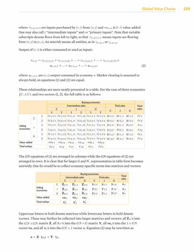
where where z(s,j),(r,i) are inputs purchased by (r, i) from (s, j) and va(r,i) is (r, i) value-added. One may also callz “intermediate inputs” and va “primary inputs”. Note that variable subscripts denote flows from left toright, so that z(s,j),(r,i) means inputs are flowing from (s, j) to (r, i). An asterisk means all entities, as inz(s,j),∗ or z∗,(r,i).
Output of (r, i) is either consumed or used as inputs:
x(r,i) = z(r,i),(1,1) + z(r,i),(1,2) + ... + z(r,i),(u,i) + ... + z(r,i),(G,N)+
y(r,i),1 + ... + y(r,i),u + ... + y(r,i),G, (2)
where y(r,i),u are (r, i) output consumed in economy u. Market clearing is assumed to always hold, soequations (1) and (2) are equal.
These relationships are more neatly presented in a table. For the case of three economies {C, J, U} and twosectors {1, 2}, the full table is as follows:
Buying economiesTotalsales
Intermediate sales Final salesC J U
C J U1 2 1 2 1 2
Sellingeconomies
C1 zC1,C1 zC1,C2 zC1,J1 zC1,J2 zC1,U1 zC1,U2 yC1,C yC1,J yC1,U xC1
2 zC2,C1 zC2,C2 zC2,J1 zC2,J2 zC2,U1 zC2,U2 yC2,C yC2,J yC2,U xC2
J1 zJ1,C1 zJ1,C2 zJ1,J1 zJ1,J2 zJ1,U1 zJ1,U2 yJ1,C yJ1,J yJ1,U xJ1
2 zJ2,C1 zJ2,C2 zJ2,J1 zJ2,J2 zJ2,U1 zJ2,U2 yJ2,C yJ2,J yJ2,U xJ2
U1 zU1,C1 zU1,C2 zU1,J1 zU1,J2 zU1,U1 zU1,U2 yU1,C yU1,J yU1,U xU1
2 zU2,C1 zU2,C2 zU2,J1 zU2,J2 zU2,U1 zU2,U2 yU2,C yU2,J yU2,U xU2
Value-added vaC1 vaC2 vaJ1 vaJ2 vaU1 vaU2
Total outlays xC1 xC2 xJ1 xJ2 xU1 xU2
The GN equations of (1) are arranged in columns while the GN equations of (2) are arranged in rows. It isclear that for larger G and N , representation in table form becomes unwieldy. One fix would be to collecteconomy-specific terms into matrices and vectors:
Buying economiesTotal salesIntermediate sales Final sales
C J U C J U
Selling economiesC ZCC ZCJ ZCU yCC yCJ yCU xC
J ZJC ZJJ ZJU yJC yJJ yJU xJ
U ZUC ZUJ ZUU yUC yUJ yUU xU
Value-added vaC vaJ vaU
Total outlays x′C x′
J x′U
Uppercase letters in bold denote matrices while lowercase letters in bold denote vectors. These may furtherbe collected into larger matrices and vectors: all Zsr’s into the GN ×GN matrix Z, all ysr’s into the GN ×G
2
are inputs purchased by where z(s,j),(r,i) are inputs purchased by (r, i) from (s, j) and va(r,i) is (r, i) value-added. One may also callz “intermediate inputs” and va “primary inputs”. Note that variable subscripts denote flows from left toright, so that z(s,j),(r,i) means inputs are flowing from (s, j) to (r, i). An asterisk means all entities, as inz(s,j),∗ or z∗,(r,i).
Output of (r, i) is either consumed or used as inputs:
x(r,i) = z(r,i),(1,1) + z(r,i),(1,2) + ... + z(r,i),(u,i) + ... + z(r,i),(G,N)+
y(r,i),1 + ... + y(r,i),u + ... + y(r,i),G, (2)
where y(r,i),u are (r, i) output consumed in economy u. Market clearing is assumed to always hold, soequations (1) and (2) are equal.
These relationships are more neatly presented in a table. For the case of three economies {C, J, U} and twosectors {1, 2}, the full table is as follows:
Buying economiesTotalsales
Intermediate sales Final salesC J U
C J U1 2 1 2 1 2
Sellingeconomies
C1 zC1,C1 zC1,C2 zC1,J1 zC1,J2 zC1,U1 zC1,U2 yC1,C yC1,J yC1,U xC1
2 zC2,C1 zC2,C2 zC2,J1 zC2,J2 zC2,U1 zC2,U2 yC2,C yC2,J yC2,U xC2
J1 zJ1,C1 zJ1,C2 zJ1,J1 zJ1,J2 zJ1,U1 zJ1,U2 yJ1,C yJ1,J yJ1,U xJ1
2 zJ2,C1 zJ2,C2 zJ2,J1 zJ2,J2 zJ2,U1 zJ2,U2 yJ2,C yJ2,J yJ2,U xJ2
U1 zU1,C1 zU1,C2 zU1,J1 zU1,J2 zU1,U1 zU1,U2 yU1,C yU1,J yU1,U xU1
2 zU2,C1 zU2,C2 zU2,J1 zU2,J2 zU2,U1 zU2,U2 yU2,C yU2,J yU2,U xU2
Value-added vaC1 vaC2 vaJ1 vaJ2 vaU1 vaU2
Total outlays xC1 xC2 xJ1 xJ2 xU1 xU2
The GN equations of (1) are arranged in columns while the GN equations of (2) are arranged in rows. It isclear that for larger G and N , representation in table form becomes unwieldy. One fix would be to collecteconomy-specific terms into matrices and vectors:
Buying economiesTotal salesIntermediate sales Final sales
C J U C J U
Selling economiesC ZCC ZCJ ZCU yCC yCJ yCU xC
J ZJC ZJJ ZJU yJC yJJ yJU xJ
U ZUC ZUJ ZUU yUC yUJ yUU xU
Value-added vaC vaJ vaU
Total outlays x′C x′
J x′U
Uppercase letters in bold denote matrices while lowercase letters in bold denote vectors. These may furtherbe collected into larger matrices and vectors: all Zsr’s into the GN ×GN matrix Z, all ysr’s into the GN ×G
2
from where z(s,j),(r,i) are inputs purchased by (r, i) from (s, j) and va(r,i) is (r, i) value-added. One may also callz “intermediate inputs” and va “primary inputs”. Note that variable subscripts denote flows from left toright, so that z(s,j),(r,i) means inputs are flowing from (s, j) to (r, i). An asterisk means all entities, as inz(s,j),∗ or z∗,(r,i).
Output of (r, i) is either consumed or used as inputs:
x(r,i) = z(r,i),(1,1) + z(r,i),(1,2) + ... + z(r,i),(u,i) + ... + z(r,i),(G,N)+
y(r,i),1 + ... + y(r,i),u + ... + y(r,i),G, (2)
where y(r,i),u are (r, i) output consumed in economy u. Market clearing is assumed to always hold, soequations (1) and (2) are equal.
These relationships are more neatly presented in a table. For the case of three economies {C, J, U} and twosectors {1, 2}, the full table is as follows:
Buying economiesTotalsales
Intermediate sales Final salesC J U
C J U1 2 1 2 1 2
Sellingeconomies
C1 zC1,C1 zC1,C2 zC1,J1 zC1,J2 zC1,U1 zC1,U2 yC1,C yC1,J yC1,U xC1
2 zC2,C1 zC2,C2 zC2,J1 zC2,J2 zC2,U1 zC2,U2 yC2,C yC2,J yC2,U xC2
J1 zJ1,C1 zJ1,C2 zJ1,J1 zJ1,J2 zJ1,U1 zJ1,U2 yJ1,C yJ1,J yJ1,U xJ1
2 zJ2,C1 zJ2,C2 zJ2,J1 zJ2,J2 zJ2,U1 zJ2,U2 yJ2,C yJ2,J yJ2,U xJ2
U1 zU1,C1 zU1,C2 zU1,J1 zU1,J2 zU1,U1 zU1,U2 yU1,C yU1,J yU1,U xU1
2 zU2,C1 zU2,C2 zU2,J1 zU2,J2 zU2,U1 zU2,U2 yU2,C yU2,J yU2,U xU2
Value-added vaC1 vaC2 vaJ1 vaJ2 vaU1 vaU2
Total outlays xC1 xC2 xJ1 xJ2 xU1 xU2
The GN equations of (1) are arranged in columns while the GN equations of (2) are arranged in rows. It isclear that for larger G and N , representation in table form becomes unwieldy. One fix would be to collecteconomy-specific terms into matrices and vectors:
Buying economiesTotal salesIntermediate sales Final sales
C J U C J U
Selling economiesC ZCC ZCJ ZCU yCC yCJ yCU xC
J ZJC ZJJ ZJU yJC yJJ yJU xJ
U ZUC ZUJ ZUU yUC yUJ yUU xU
Value-added vaC vaJ vaU
Total outlays x′C x′
J x′U
Uppercase letters in bold denote matrices while lowercase letters in bold denote vectors. These may furtherbe collected into larger matrices and vectors: all Zsr’s into the GN ×GN matrix Z, all ysr’s into the GN ×G
2
and where z(s,j),(r,i) are inputs purchased by (r, i) from (s, j) and va(r,i) is (r, i) value-added. One may also callz “intermediate inputs” and va “primary inputs”. Note that variable subscripts denote flows from left toright, so that z(s,j),(r,i) means inputs are flowing from (s, j) to (r, i). An asterisk means all entities, as inz(s,j),∗ or z∗,(r,i).
Output of (r, i) is either consumed or used as inputs:
x(r,i) = z(r,i),(1,1) + z(r,i),(1,2) + ... + z(r,i),(u,i) + ... + z(r,i),(G,N)+
y(r,i),1 + ... + y(r,i),u + ... + y(r,i),G, (2)
where y(r,i),u are (r, i) output consumed in economy u. Market clearing is assumed to always hold, soequations (1) and (2) are equal.
These relationships are more neatly presented in a table. For the case of three economies {C, J, U} and twosectors {1, 2}, the full table is as follows:
Buying economiesTotalsales
Intermediate sales Final salesC J U
C J U1 2 1 2 1 2
Sellingeconomies
C1 zC1,C1 zC1,C2 zC1,J1 zC1,J2 zC1,U1 zC1,U2 yC1,C yC1,J yC1,U xC1
2 zC2,C1 zC2,C2 zC2,J1 zC2,J2 zC2,U1 zC2,U2 yC2,C yC2,J yC2,U xC2
J1 zJ1,C1 zJ1,C2 zJ1,J1 zJ1,J2 zJ1,U1 zJ1,U2 yJ1,C yJ1,J yJ1,U xJ1
2 zJ2,C1 zJ2,C2 zJ2,J1 zJ2,J2 zJ2,U1 zJ2,U2 yJ2,C yJ2,J yJ2,U xJ2
U1 zU1,C1 zU1,C2 zU1,J1 zU1,J2 zU1,U1 zU1,U2 yU1,C yU1,J yU1,U xU1
2 zU2,C1 zU2,C2 zU2,J1 zU2,J2 zU2,U1 zU2,U2 yU2,C yU2,J yU2,U xU2
Value-added vaC1 vaC2 vaJ1 vaJ2 vaU1 vaU2
Total outlays xC1 xC2 xJ1 xJ2 xU1 xU2
The GN equations of (1) are arranged in columns while the GN equations of (2) are arranged in rows. It isclear that for larger G and N , representation in table form becomes unwieldy. One fix would be to collecteconomy-specific terms into matrices and vectors:
Buying economiesTotal salesIntermediate sales Final sales
C J U C J U
Selling economiesC ZCC ZCJ ZCU yCC yCJ yCU xC
J ZJC ZJJ ZJU yJC yJJ yJU xJ
U ZUC ZUJ ZUU yUC yUJ yUU xU
Value-added vaC vaJ vaU
Total outlays x′C x′
J x′U
Uppercase letters in bold denote matrices while lowercase letters in bold denote vectors. These may furtherbe collected into larger matrices and vectors: all Zsr’s into the GN ×GN matrix Z, all ysr’s into the GN ×G
2
is where z(s,j),(r,i) are inputs purchased by (r, i) from (s, j) and va(r,i) is (r, i) value-added. One may also callz “intermediate inputs” and va “primary inputs”. Note that variable subscripts denote flows from left toright, so that z(s,j),(r,i) means inputs are flowing from (s, j) to (r, i). An asterisk means all entities, as inz(s,j),∗ or z∗,(r,i).
Output of (r, i) is either consumed or used as inputs:
x(r,i) = z(r,i),(1,1) + z(r,i),(1,2) + ... + z(r,i),(u,i) + ... + z(r,i),(G,N)+
y(r,i),1 + ... + y(r,i),u + ... + y(r,i),G, (2)
where y(r,i),u are (r, i) output consumed in economy u. Market clearing is assumed to always hold, soequations (1) and (2) are equal.
These relationships are more neatly presented in a table. For the case of three economies {C, J, U} and twosectors {1, 2}, the full table is as follows:
Buying economiesTotalsales
Intermediate sales Final salesC J U
C J U1 2 1 2 1 2
Sellingeconomies
C1 zC1,C1 zC1,C2 zC1,J1 zC1,J2 zC1,U1 zC1,U2 yC1,C yC1,J yC1,U xC1
2 zC2,C1 zC2,C2 zC2,J1 zC2,J2 zC2,U1 zC2,U2 yC2,C yC2,J yC2,U xC2
J1 zJ1,C1 zJ1,C2 zJ1,J1 zJ1,J2 zJ1,U1 zJ1,U2 yJ1,C yJ1,J yJ1,U xJ1
2 zJ2,C1 zJ2,C2 zJ2,J1 zJ2,J2 zJ2,U1 zJ2,U2 yJ2,C yJ2,J yJ2,U xJ2
U1 zU1,C1 zU1,C2 zU1,J1 zU1,J2 zU1,U1 zU1,U2 yU1,C yU1,J yU1,U xU1
2 zU2,C1 zU2,C2 zU2,J1 zU2,J2 zU2,U1 zU2,U2 yU2,C yU2,J yU2,U xU2
Value-added vaC1 vaC2 vaJ1 vaJ2 vaU1 vaU2
Total outlays xC1 xC2 xJ1 xJ2 xU1 xU2
The GN equations of (1) are arranged in columns while the GN equations of (2) are arranged in rows. It isclear that for larger G and N , representation in table form becomes unwieldy. One fix would be to collecteconomy-specific terms into matrices and vectors:
Buying economiesTotal salesIntermediate sales Final sales
C J U C J U
Selling economiesC ZCC ZCJ ZCU yCC yCJ yCU xC
J ZJC ZJJ ZJU yJC yJJ yJU xJ
U ZUC ZUJ ZUU yUC yUJ yUU xU
Value-added vaC vaJ vaU
Total outlays x′C x′
J x′U
Uppercase letters in bold denote matrices while lowercase letters in bold denote vectors. These may furtherbe collected into larger matrices and vectors: all Zsr’s into the GN ×GN matrix Z, all ysr’s into the GN ×G
2
value-added. One may also call
where z(s,j),(r,i) are inputs purchased by (r, i) from (s, j) and va(r,i) is (r, i) value-added. One may also callz “intermediate inputs” and va “primary inputs”. Note that variable subscripts denote flows from left toright, so that z(s,j),(r,i) means inputs are flowing from (s, j) to (r, i). An asterisk means all entities, as inz(s,j),∗ or z∗,(r,i).
Output of (r, i) is either consumed or used as inputs:
x(r,i) = z(r,i),(1,1) + z(r,i),(1,2) + ... + z(r,i),(u,i) + ... + z(r,i),(G,N)+
y(r,i),1 + ... + y(r,i),u + ... + y(r,i),G, (2)
where y(r,i),u are (r, i) output consumed in economy u. Market clearing is assumed to always hold, soequations (1) and (2) are equal.
These relationships are more neatly presented in a table. For the case of three economies {C, J, U} and twosectors {1, 2}, the full table is as follows:
Buying economiesTotalsales
Intermediate sales Final salesC J U
C J U1 2 1 2 1 2
Sellingeconomies
C1 zC1,C1 zC1,C2 zC1,J1 zC1,J2 zC1,U1 zC1,U2 yC1,C yC1,J yC1,U xC1
2 zC2,C1 zC2,C2 zC2,J1 zC2,J2 zC2,U1 zC2,U2 yC2,C yC2,J yC2,U xC2
J1 zJ1,C1 zJ1,C2 zJ1,J1 zJ1,J2 zJ1,U1 zJ1,U2 yJ1,C yJ1,J yJ1,U xJ1
2 zJ2,C1 zJ2,C2 zJ2,J1 zJ2,J2 zJ2,U1 zJ2,U2 yJ2,C yJ2,J yJ2,U xJ2
U1 zU1,C1 zU1,C2 zU1,J1 zU1,J2 zU1,U1 zU1,U2 yU1,C yU1,J yU1,U xU1
2 zU2,C1 zU2,C2 zU2,J1 zU2,J2 zU2,U1 zU2,U2 yU2,C yU2,J yU2,U xU2
Value-added vaC1 vaC2 vaJ1 vaJ2 vaU1 vaU2
Total outlays xC1 xC2 xJ1 xJ2 xU1 xU2
The GN equations of (1) are arranged in columns while the GN equations of (2) are arranged in rows. It isclear that for larger G and N , representation in table form becomes unwieldy. One fix would be to collecteconomy-specific terms into matrices and vectors:
Buying economiesTotal salesIntermediate sales Final sales
C J U C J U
Selling economiesC ZCC ZCJ ZCU yCC yCJ yCU xC
J ZJC ZJJ ZJU yJC yJJ yJU xJ
U ZUC ZUJ ZUU yUC yUJ yUU xU
Value-added vaC vaJ vaU
Total outlays x′C x′
J x′U
Uppercase letters in bold denote matrices while lowercase letters in bold denote vectors. These may furtherbe collected into larger matrices and vectors: all Zsr’s into the GN ×GN matrix Z, all ysr’s into the GN ×G
2
“intermediate inputs” and where z(s,j),(r,i) are inputs purchased by (r, i) from (s, j) and va(r,i) is (r, i) value-added. One may also callz “intermediate inputs” and va “primary inputs”. Note that variable subscripts denote flows from left toright, so that z(s,j),(r,i) means inputs are flowing from (s, j) to (r, i). An asterisk means all entities, as inz(s,j),∗ or z∗,(r,i).
Output of (r, i) is either consumed or used as inputs:
x(r,i) = z(r,i),(1,1) + z(r,i),(1,2) + ... + z(r,i),(u,i) + ... + z(r,i),(G,N)+
y(r,i),1 + ... + y(r,i),u + ... + y(r,i),G, (2)
where y(r,i),u are (r, i) output consumed in economy u. Market clearing is assumed to always hold, soequations (1) and (2) are equal.
These relationships are more neatly presented in a table. For the case of three economies {C, J, U} and twosectors {1, 2}, the full table is as follows:
Buying economiesTotalsales
Intermediate sales Final salesC J U
C J U1 2 1 2 1 2
Sellingeconomies
C1 zC1,C1 zC1,C2 zC1,J1 zC1,J2 zC1,U1 zC1,U2 yC1,C yC1,J yC1,U xC1
2 zC2,C1 zC2,C2 zC2,J1 zC2,J2 zC2,U1 zC2,U2 yC2,C yC2,J yC2,U xC2
J1 zJ1,C1 zJ1,C2 zJ1,J1 zJ1,J2 zJ1,U1 zJ1,U2 yJ1,C yJ1,J yJ1,U xJ1
2 zJ2,C1 zJ2,C2 zJ2,J1 zJ2,J2 zJ2,U1 zJ2,U2 yJ2,C yJ2,J yJ2,U xJ2
U1 zU1,C1 zU1,C2 zU1,J1 zU1,J2 zU1,U1 zU1,U2 yU1,C yU1,J yU1,U xU1
2 zU2,C1 zU2,C2 zU2,J1 zU2,J2 zU2,U1 zU2,U2 yU2,C yU2,J yU2,U xU2
Value-added vaC1 vaC2 vaJ1 vaJ2 vaU1 vaU2
Total outlays xC1 xC2 xJ1 xJ2 xU1 xU2
The GN equations of (1) are arranged in columns while the GN equations of (2) are arranged in rows. It isclear that for larger G and N , representation in table form becomes unwieldy. One fix would be to collecteconomy-specific terms into matrices and vectors:
Buying economiesTotal salesIntermediate sales Final sales
C J U C J U
Selling economiesC ZCC ZCJ ZCU yCC yCJ yCU xC
J ZJC ZJJ ZJU yJC yJJ yJU xJ
U ZUC ZUJ ZUU yUC yUJ yUU xU
Value-added vaC vaJ vaU
Total outlays x′C x′
J x′U
Uppercase letters in bold denote matrices while lowercase letters in bold denote vectors. These may furtherbe collected into larger matrices and vectors: all Zsr’s into the GN ×GN matrix Z, all ysr’s into the GN ×G
2
“primary inputs”. Note that variable subscripts denote flows from left to right, so that
where z(s,j),(r,i) are inputs purchased by (r, i) from (s, j) and va(r,i) is (r, i) value-added. One may also callz “intermediate inputs” and va “primary inputs”. Note that variable subscripts denote flows from left toright, so that z(s,j),(r,i) means inputs are flowing from (s, j) to (r, i). An asterisk means all entities, as inz(s,j),∗ or z∗,(r,i).
Output of (r, i) is either consumed or used as inputs:
x(r,i) = z(r,i),(1,1) + z(r,i),(1,2) + ... + z(r,i),(u,i) + ... + z(r,i),(G,N)+
y(r,i),1 + ... + y(r,i),u + ... + y(r,i),G, (2)
where y(r,i),u are (r, i) output consumed in economy u. Market clearing is assumed to always hold, soequations (1) and (2) are equal.
These relationships are more neatly presented in a table. For the case of three economies {C, J, U} and twosectors {1, 2}, the full table is as follows:
Buying economiesTotalsales
Intermediate sales Final salesC J U
C J U1 2 1 2 1 2
Sellingeconomies
C1 zC1,C1 zC1,C2 zC1,J1 zC1,J2 zC1,U1 zC1,U2 yC1,C yC1,J yC1,U xC1
2 zC2,C1 zC2,C2 zC2,J1 zC2,J2 zC2,U1 zC2,U2 yC2,C yC2,J yC2,U xC2
J1 zJ1,C1 zJ1,C2 zJ1,J1 zJ1,J2 zJ1,U1 zJ1,U2 yJ1,C yJ1,J yJ1,U xJ1
2 zJ2,C1 zJ2,C2 zJ2,J1 zJ2,J2 zJ2,U1 zJ2,U2 yJ2,C yJ2,J yJ2,U xJ2
U1 zU1,C1 zU1,C2 zU1,J1 zU1,J2 zU1,U1 zU1,U2 yU1,C yU1,J yU1,U xU1
2 zU2,C1 zU2,C2 zU2,J1 zU2,J2 zU2,U1 zU2,U2 yU2,C yU2,J yU2,U xU2
Value-added vaC1 vaC2 vaJ1 vaJ2 vaU1 vaU2
Total outlays xC1 xC2 xJ1 xJ2 xU1 xU2
The GN equations of (1) are arranged in columns while the GN equations of (2) are arranged in rows. It isclear that for larger G and N , representation in table form becomes unwieldy. One fix would be to collecteconomy-specific terms into matrices and vectors:
Buying economiesTotal salesIntermediate sales Final sales
C J U C J U
Selling economiesC ZCC ZCJ ZCU yCC yCJ yCU xC
J ZJC ZJJ ZJU yJC yJJ yJU xJ
U ZUC ZUJ ZUU yUC yUJ yUU xU
Value-added vaC vaJ vaU
Total outlays x′C x′
J x′U
Uppercase letters in bold denote matrices while lowercase letters in bold denote vectors. These may furtherbe collected into larger matrices and vectors: all Zsr’s into the GN ×GN matrix Z, all ysr’s into the GN ×G
2
means inputs are flowing from where z(s,j),(r,i) are inputs purchased by (r, i) from (s, j) and va(r,i) is (r, i) value-added. One may also call
z “intermediate inputs” and va “primary inputs”. Note that variable subscripts denote flows from left toright, so that z(s,j),(r,i) means inputs are flowing from (s, j) to (r, i). An asterisk means all entities, as inz(s,j),∗ or z∗,(r,i).
Output of (r, i) is either consumed or used as inputs:
x(r,i) = z(r,i),(1,1) + z(r,i),(1,2) + ... + z(r,i),(u,i) + ... + z(r,i),(G,N)+
y(r,i),1 + ... + y(r,i),u + ... + y(r,i),G, (2)
where y(r,i),u are (r, i) output consumed in economy u. Market clearing is assumed to always hold, soequations (1) and (2) are equal.
These relationships are more neatly presented in a table. For the case of three economies {C, J, U} and twosectors {1, 2}, the full table is as follows:
Buying economiesTotalsales
Intermediate sales Final salesC J U
C J U1 2 1 2 1 2
Sellingeconomies
C1 zC1,C1 zC1,C2 zC1,J1 zC1,J2 zC1,U1 zC1,U2 yC1,C yC1,J yC1,U xC1
2 zC2,C1 zC2,C2 zC2,J1 zC2,J2 zC2,U1 zC2,U2 yC2,C yC2,J yC2,U xC2
J1 zJ1,C1 zJ1,C2 zJ1,J1 zJ1,J2 zJ1,U1 zJ1,U2 yJ1,C yJ1,J yJ1,U xJ1
2 zJ2,C1 zJ2,C2 zJ2,J1 zJ2,J2 zJ2,U1 zJ2,U2 yJ2,C yJ2,J yJ2,U xJ2
U1 zU1,C1 zU1,C2 zU1,J1 zU1,J2 zU1,U1 zU1,U2 yU1,C yU1,J yU1,U xU1
2 zU2,C1 zU2,C2 zU2,J1 zU2,J2 zU2,U1 zU2,U2 yU2,C yU2,J yU2,U xU2
Value-added vaC1 vaC2 vaJ1 vaJ2 vaU1 vaU2
Total outlays xC1 xC2 xJ1 xJ2 xU1 xU2
The GN equations of (1) are arranged in columns while the GN equations of (2) are arranged in rows. It isclear that for larger G and N , representation in table form becomes unwieldy. One fix would be to collecteconomy-specific terms into matrices and vectors:
Buying economiesTotal salesIntermediate sales Final sales
C J U C J U
Selling economiesC ZCC ZCJ ZCU yCC yCJ yCU xC
J ZJC ZJJ ZJU yJC yJJ yJU xJ
U ZUC ZUJ ZUU yUC yUJ yUU xU
Value-added vaC vaJ vaU
Total outlays x′C x′
J x′U
Uppercase letters in bold denote matrices while lowercase letters in bold denote vectors. These may furtherbe collected into larger matrices and vectors: all Zsr’s into the GN ×GN matrix Z, all ysr’s into the GN ×G
2
to where z(s,j),(r,i) are inputs purchased by (r, i) from (s, j) and va(r,i) is (r, i) value-added. One may also callz “intermediate inputs” and va “primary inputs”. Note that variable subscripts denote flows from left toright, so that z(s,j),(r,i) means inputs are flowing from (s, j) to (r, i). An asterisk means all entities, as inz(s,j),∗ or z∗,(r,i).
Output of (r, i) is either consumed or used as inputs:
x(r,i) = z(r,i),(1,1) + z(r,i),(1,2) + ... + z(r,i),(u,i) + ... + z(r,i),(G,N)+
y(r,i),1 + ... + y(r,i),u + ... + y(r,i),G, (2)
where y(r,i),u are (r, i) output consumed in economy u. Market clearing is assumed to always hold, soequations (1) and (2) are equal.
These relationships are more neatly presented in a table. For the case of three economies {C, J, U} and twosectors {1, 2}, the full table is as follows:
Buying economiesTotalsales
Intermediate sales Final salesC J U
C J U1 2 1 2 1 2
Sellingeconomies
C1 zC1,C1 zC1,C2 zC1,J1 zC1,J2 zC1,U1 zC1,U2 yC1,C yC1,J yC1,U xC1
2 zC2,C1 zC2,C2 zC2,J1 zC2,J2 zC2,U1 zC2,U2 yC2,C yC2,J yC2,U xC2
J1 zJ1,C1 zJ1,C2 zJ1,J1 zJ1,J2 zJ1,U1 zJ1,U2 yJ1,C yJ1,J yJ1,U xJ1
2 zJ2,C1 zJ2,C2 zJ2,J1 zJ2,J2 zJ2,U1 zJ2,U2 yJ2,C yJ2,J yJ2,U xJ2
U1 zU1,C1 zU1,C2 zU1,J1 zU1,J2 zU1,U1 zU1,U2 yU1,C yU1,J yU1,U xU1
2 zU2,C1 zU2,C2 zU2,J1 zU2,J2 zU2,U1 zU2,U2 yU2,C yU2,J yU2,U xU2
Value-added vaC1 vaC2 vaJ1 vaJ2 vaU1 vaU2
Total outlays xC1 xC2 xJ1 xJ2 xU1 xU2
The GN equations of (1) are arranged in columns while the GN equations of (2) are arranged in rows. It isclear that for larger G and N , representation in table form becomes unwieldy. One fix would be to collecteconomy-specific terms into matrices and vectors:
Buying economiesTotal salesIntermediate sales Final sales
C J U C J U
Selling economiesC ZCC ZCJ ZCU yCC yCJ yCU xC
J ZJC ZJJ ZJU yJC yJJ yJU xJ
U ZUC ZUJ ZUU yUC yUJ yUU xU
Value-added vaC vaJ vaU
Total outlays x′C x′
J x′U
Uppercase letters in bold denote matrices while lowercase letters in bold denote vectors. These may furtherbe collected into larger matrices and vectors: all Zsr’s into the GN ×GN matrix Z, all ysr’s into the GN ×G
2
. An asterisk means all entities, as in
where z(s,j),(r,i) are inputs purchased by (r, i) from (s, j) and va(r,i) is (r, i) value-added. One may also callz “intermediate inputs” and va “primary inputs”. Note that variable subscripts denote flows from left toright, so that z(s,j),(r,i) means inputs are flowing from (s, j) to (r, i). An asterisk means all entities, as inz(s,j),∗ or z∗,(r,i).
Output of (r, i) is either consumed or used as inputs:
x(r,i) = z(r,i),(1,1) + z(r,i),(1,2) + ... + z(r,i),(u,i) + ... + z(r,i),(G,N)+
y(r,i),1 + ... + y(r,i),u + ... + y(r,i),G, (2)
where y(r,i),u are (r, i) output consumed in economy u. Market clearing is assumed to always hold, soequations (1) and (2) are equal.
These relationships are more neatly presented in a table. For the case of three economies {C, J, U} and twosectors {1, 2}, the full table is as follows:
Buying economiesTotalsales
Intermediate sales Final salesC J U
C J U1 2 1 2 1 2
Sellingeconomies
C1 zC1,C1 zC1,C2 zC1,J1 zC1,J2 zC1,U1 zC1,U2 yC1,C yC1,J yC1,U xC1
2 zC2,C1 zC2,C2 zC2,J1 zC2,J2 zC2,U1 zC2,U2 yC2,C yC2,J yC2,U xC2
J1 zJ1,C1 zJ1,C2 zJ1,J1 zJ1,J2 zJ1,U1 zJ1,U2 yJ1,C yJ1,J yJ1,U xJ1
2 zJ2,C1 zJ2,C2 zJ2,J1 zJ2,J2 zJ2,U1 zJ2,U2 yJ2,C yJ2,J yJ2,U xJ2
U1 zU1,C1 zU1,C2 zU1,J1 zU1,J2 zU1,U1 zU1,U2 yU1,C yU1,J yU1,U xU1
2 zU2,C1 zU2,C2 zU2,J1 zU2,J2 zU2,U1 zU2,U2 yU2,C yU2,J yU2,U xU2
Value-added vaC1 vaC2 vaJ1 vaJ2 vaU1 vaU2
Total outlays xC1 xC2 xJ1 xJ2 xU1 xU2
The GN equations of (1) are arranged in columns while the GN equations of (2) are arranged in rows. It isclear that for larger G and N , representation in table form becomes unwieldy. One fix would be to collecteconomy-specific terms into matrices and vectors:
Buying economiesTotal salesIntermediate sales Final sales
C J U C J U
Selling economiesC ZCC ZCJ ZCU yCC yCJ yCU xC
J ZJC ZJJ ZJU yJC yJJ yJU xJ
U ZUC ZUJ ZUU yUC yUJ yUU xU
Value-added vaC vaJ vaU
Total outlays x′C x′
J x′U
Uppercase letters in bold denote matrices while lowercase letters in bold denote vectors. These may furtherbe collected into larger matrices and vectors: all Zsr’s into the GN ×GN matrix Z, all ysr’s into the GN ×G
2
or
where z(s,j),(r,i) are inputs purchased by (r, i) from (s, j) and va(r,i) is (r, i) value-added. One may also callz “intermediate inputs” and va “primary inputs”. Note that variable subscripts denote flows from left toright, so that z(s,j),(r,i) means inputs are flowing from (s, j) to (r, i). An asterisk means all entities, as inz(s,j),∗ or z∗,(r,i).
Output of (r, i) is either consumed or used as inputs:
x(r,i) = z(r,i),(1,1) + z(r,i),(1,2) + ... + z(r,i),(u,i) + ... + z(r,i),(G,N)+
y(r,i),1 + ... + y(r,i),u + ... + y(r,i),G, (2)
where y(r,i),u are (r, i) output consumed in economy u. Market clearing is assumed to always hold, soequations (1) and (2) are equal.
These relationships are more neatly presented in a table. For the case of three economies {C, J, U} and twosectors {1, 2}, the full table is as follows:
Buying economiesTotalsales
Intermediate sales Final salesC J U
C J U1 2 1 2 1 2
Sellingeconomies
C1 zC1,C1 zC1,C2 zC1,J1 zC1,J2 zC1,U1 zC1,U2 yC1,C yC1,J yC1,U xC1
2 zC2,C1 zC2,C2 zC2,J1 zC2,J2 zC2,U1 zC2,U2 yC2,C yC2,J yC2,U xC2
J1 zJ1,C1 zJ1,C2 zJ1,J1 zJ1,J2 zJ1,U1 zJ1,U2 yJ1,C yJ1,J yJ1,U xJ1
2 zJ2,C1 zJ2,C2 zJ2,J1 zJ2,J2 zJ2,U1 zJ2,U2 yJ2,C yJ2,J yJ2,U xJ2
U1 zU1,C1 zU1,C2 zU1,J1 zU1,J2 zU1,U1 zU1,U2 yU1,C yU1,J yU1,U xU1
2 zU2,C1 zU2,C2 zU2,J1 zU2,J2 zU2,U1 zU2,U2 yU2,C yU2,J yU2,U xU2
Value-added vaC1 vaC2 vaJ1 vaJ2 vaU1 vaU2
Total outlays xC1 xC2 xJ1 xJ2 xU1 xU2
The GN equations of (1) are arranged in columns while the GN equations of (2) are arranged in rows. It isclear that for larger G and N , representation in table form becomes unwieldy. One fix would be to collecteconomy-specific terms into matrices and vectors:
Buying economiesTotal salesIntermediate sales Final sales
C J U C J U
Selling economiesC ZCC ZCJ ZCU yCC yCJ yCU xC
J ZJC ZJJ ZJU yJC yJJ yJU xJ
U ZUC ZUJ ZUU yUC yUJ yUU xU
Value-added vaC vaJ vaU
Total outlays x′C x′
J x′U
Uppercase letters in bold denote matrices while lowercase letters in bold denote vectors. These may furtherbe collected into larger matrices and vectors: all Zsr’s into the GN ×GN matrix Z, all ysr’s into the GN ×G
2
.
Output of where z(s,j),(r,i) are inputs purchased by (r, i) from (s, j) and va(r,i) is (r, i) value-added. One may also callz “intermediate inputs” and va “primary inputs”. Note that variable subscripts denote flows from left toright, so that z(s,j),(r,i) means inputs are flowing from (s, j) to (r, i). An asterisk means all entities, as inz(s,j),∗ or z∗,(r,i).
Output of (r, i) is either consumed or used as inputs:
x(r,i) = z(r,i),(1,1) + z(r,i),(1,2) + ... + z(r,i),(u,i) + ... + z(r,i),(G,N)+
y(r,i),1 + ... + y(r,i),u + ... + y(r,i),G, (2)
where y(r,i),u are (r, i) output consumed in economy u. Market clearing is assumed to always hold, soequations (1) and (2) are equal.
These relationships are more neatly presented in a table. For the case of three economies {C, J, U} and twosectors {1, 2}, the full table is as follows:
Buying economiesTotalsales
Intermediate sales Final salesC J U
C J U1 2 1 2 1 2
Sellingeconomies
C1 zC1,C1 zC1,C2 zC1,J1 zC1,J2 zC1,U1 zC1,U2 yC1,C yC1,J yC1,U xC1
2 zC2,C1 zC2,C2 zC2,J1 zC2,J2 zC2,U1 zC2,U2 yC2,C yC2,J yC2,U xC2
J1 zJ1,C1 zJ1,C2 zJ1,J1 zJ1,J2 zJ1,U1 zJ1,U2 yJ1,C yJ1,J yJ1,U xJ1
2 zJ2,C1 zJ2,C2 zJ2,J1 zJ2,J2 zJ2,U1 zJ2,U2 yJ2,C yJ2,J yJ2,U xJ2
U1 zU1,C1 zU1,C2 zU1,J1 zU1,J2 zU1,U1 zU1,U2 yU1,C yU1,J yU1,U xU1
2 zU2,C1 zU2,C2 zU2,J1 zU2,J2 zU2,U1 zU2,U2 yU2,C yU2,J yU2,U xU2
Value-added vaC1 vaC2 vaJ1 vaJ2 vaU1 vaU2
Total outlays xC1 xC2 xJ1 xJ2 xU1 xU2
The GN equations of (1) are arranged in columns while the GN equations of (2) are arranged in rows. It isclear that for larger G and N , representation in table form becomes unwieldy. One fix would be to collecteconomy-specific terms into matrices and vectors:
Buying economiesTotal salesIntermediate sales Final sales
C J U C J U
Selling economiesC ZCC ZCJ ZCU yCC yCJ yCU xC
J ZJC ZJJ ZJU yJC yJJ yJU xJ
U ZUC ZUJ ZUU yUC yUJ yUU xU
Value-added vaC vaJ vaU
Total outlays x′C x′
J x′U
Uppercase letters in bold denote matrices while lowercase letters in bold denote vectors. These may furtherbe collected into larger matrices and vectors: all Zsr’s into the GN ×GN matrix Z, all ysr’s into the GN ×G
2
is either consumed or used as inputs:
where z(s,j),(r,i) are inputs purchased by (r, i) from (s, j) and va(r,i) is (r, i) value-added. One may also callz “intermediate inputs” and va “primary inputs”. Note that variable subscripts denote flows from left toright, so that z(s,j),(r,i) means inputs are flowing from (s, j) to (r, i). An asterisk means all entities, as inz(s,j),∗ or z∗,(r,i).
Output of (r, i) is either consumed or used as inputs:
x(r,i) = z(r,i),(1,1) + z(r,i),(1,2) + ... + z(r,i),(u,i) + ... + z(r,i),(G,N)+
y(r,i),1 + ... + y(r,i),u + ... + y(r,i),G, (2)
where y(r,i),u are (r, i) output consumed in economy u. Market clearing is assumed to always hold, soequations (1) and (2) are equal.
These relationships are more neatly presented in a table. For the case of three economies {C, J, U} and twosectors {1, 2}, the full table is as follows:
Buying economiesTotalsales
Intermediate sales Final salesC J U
C J U1 2 1 2 1 2
Sellingeconomies
C1 zC1,C1 zC1,C2 zC1,J1 zC1,J2 zC1,U1 zC1,U2 yC1,C yC1,J yC1,U xC1
2 zC2,C1 zC2,C2 zC2,J1 zC2,J2 zC2,U1 zC2,U2 yC2,C yC2,J yC2,U xC2
J1 zJ1,C1 zJ1,C2 zJ1,J1 zJ1,J2 zJ1,U1 zJ1,U2 yJ1,C yJ1,J yJ1,U xJ1
2 zJ2,C1 zJ2,C2 zJ2,J1 zJ2,J2 zJ2,U1 zJ2,U2 yJ2,C yJ2,J yJ2,U xJ2
U1 zU1,C1 zU1,C2 zU1,J1 zU1,J2 zU1,U1 zU1,U2 yU1,C yU1,J yU1,U xU1
2 zU2,C1 zU2,C2 zU2,J1 zU2,J2 zU2,U1 zU2,U2 yU2,C yU2,J yU2,U xU2
Value-added vaC1 vaC2 vaJ1 vaJ2 vaU1 vaU2
Total outlays xC1 xC2 xJ1 xJ2 xU1 xU2
The GN equations of (1) are arranged in columns while the GN equations of (2) are arranged in rows. It isclear that for larger G and N , representation in table form becomes unwieldy. One fix would be to collecteconomy-specific terms into matrices and vectors:
Buying economiesTotal salesIntermediate sales Final sales
C J U C J U
Selling economiesC ZCC ZCJ ZCU yCC yCJ yCU xC
J ZJC ZJJ ZJU yJC yJJ yJU xJ
U ZUC ZUJ ZUU yUC yUJ yUU xU
Value-added vaC vaJ vaU
Total outlays x′C x′
J x′U
Uppercase letters in bold denote matrices while lowercase letters in bold denote vectors. These may furtherbe collected into larger matrices and vectors: all Zsr’s into the GN ×GN matrix Z, all ysr’s into the GN ×G
2
(2)
where
where z(s,j),(r,i) are inputs purchased by (r, i) from (s, j) and va(r,i) is (r, i) value-added. One may also callz “intermediate inputs” and va “primary inputs”. Note that variable subscripts denote flows from left toright, so that z(s,j),(r,i) means inputs are flowing from (s, j) to (r, i). An asterisk means all entities, as inz(s,j),∗ or z∗,(r,i).
Output of (r, i) is either consumed or used as inputs:
x(r,i) = z(r,i),(1,1) + z(r,i),(1,2) + ... + z(r,i),(u,i) + ... + z(r,i),(G,N)+
y(r,i),1 + ... + y(r,i),u + ... + y(r,i),G, (2)
where y(r,i),u are (r, i) output consumed in economy u. Market clearing is assumed to always hold, soequations (1) and (2) are equal.
These relationships are more neatly presented in a table. For the case of three economies {C, J, U} and twosectors {1, 2}, the full table is as follows:
Buying economiesTotalsales
Intermediate sales Final salesC J U
C J U1 2 1 2 1 2
Sellingeconomies
C1 zC1,C1 zC1,C2 zC1,J1 zC1,J2 zC1,U1 zC1,U2 yC1,C yC1,J yC1,U xC1
2 zC2,C1 zC2,C2 zC2,J1 zC2,J2 zC2,U1 zC2,U2 yC2,C yC2,J yC2,U xC2
J1 zJ1,C1 zJ1,C2 zJ1,J1 zJ1,J2 zJ1,U1 zJ1,U2 yJ1,C yJ1,J yJ1,U xJ1
2 zJ2,C1 zJ2,C2 zJ2,J1 zJ2,J2 zJ2,U1 zJ2,U2 yJ2,C yJ2,J yJ2,U xJ2
U1 zU1,C1 zU1,C2 zU1,J1 zU1,J2 zU1,U1 zU1,U2 yU1,C yU1,J yU1,U xU1
2 zU2,C1 zU2,C2 zU2,J1 zU2,J2 zU2,U1 zU2,U2 yU2,C yU2,J yU2,U xU2
Value-added vaC1 vaC2 vaJ1 vaJ2 vaU1 vaU2
Total outlays xC1 xC2 xJ1 xJ2 xU1 xU2
The GN equations of (1) are arranged in columns while the GN equations of (2) are arranged in rows. It isclear that for larger G and N , representation in table form becomes unwieldy. One fix would be to collecteconomy-specific terms into matrices and vectors:
Buying economiesTotal salesIntermediate sales Final sales
C J U C J U
Selling economiesC ZCC ZCJ ZCU yCC yCJ yCU xC
J ZJC ZJJ ZJU yJC yJJ yJU xJ
U ZUC ZUJ ZUU yUC yUJ yUU xU
Value-added vaC vaJ vaU
Total outlays x′C x′
J x′U
Uppercase letters in bold denote matrices while lowercase letters in bold denote vectors. These may furtherbe collected into larger matrices and vectors: all Zsr’s into the GN ×GN matrix Z, all ysr’s into the GN ×G
2
are where z(s,j),(r,i) are inputs purchased by (r, i) from (s, j) and va(r,i) is (r, i) value-added. One may also callz “intermediate inputs” and va “primary inputs”. Note that variable subscripts denote flows from left toright, so that z(s,j),(r,i) means inputs are flowing from (s, j) to (r, i). An asterisk means all entities, as inz(s,j),∗ or z∗,(r,i).
Output of (r, i) is either consumed or used as inputs:
x(r,i) = z(r,i),(1,1) + z(r,i),(1,2) + ... + z(r,i),(u,i) + ... + z(r,i),(G,N)+
y(r,i),1 + ... + y(r,i),u + ... + y(r,i),G, (2)
where y(r,i),u are (r, i) output consumed in economy u. Market clearing is assumed to always hold, soequations (1) and (2) are equal.
These relationships are more neatly presented in a table. For the case of three economies {C, J, U} and twosectors {1, 2}, the full table is as follows:
Buying economiesTotalsales
Intermediate sales Final salesC J U
C J U1 2 1 2 1 2
Sellingeconomies
C1 zC1,C1 zC1,C2 zC1,J1 zC1,J2 zC1,U1 zC1,U2 yC1,C yC1,J yC1,U xC1
2 zC2,C1 zC2,C2 zC2,J1 zC2,J2 zC2,U1 zC2,U2 yC2,C yC2,J yC2,U xC2
J1 zJ1,C1 zJ1,C2 zJ1,J1 zJ1,J2 zJ1,U1 zJ1,U2 yJ1,C yJ1,J yJ1,U xJ1
2 zJ2,C1 zJ2,C2 zJ2,J1 zJ2,J2 zJ2,U1 zJ2,U2 yJ2,C yJ2,J yJ2,U xJ2
U1 zU1,C1 zU1,C2 zU1,J1 zU1,J2 zU1,U1 zU1,U2 yU1,C yU1,J yU1,U xU1
2 zU2,C1 zU2,C2 zU2,J1 zU2,J2 zU2,U1 zU2,U2 yU2,C yU2,J yU2,U xU2
Value-added vaC1 vaC2 vaJ1 vaJ2 vaU1 vaU2
Total outlays xC1 xC2 xJ1 xJ2 xU1 xU2
The GN equations of (1) are arranged in columns while the GN equations of (2) are arranged in rows. It isclear that for larger G and N , representation in table form becomes unwieldy. One fix would be to collecteconomy-specific terms into matrices and vectors:
Buying economiesTotal salesIntermediate sales Final sales
C J U C J U
Selling economiesC ZCC ZCJ ZCU yCC yCJ yCU xC
J ZJC ZJJ ZJU yJC yJJ yJU xJ
U ZUC ZUJ ZUU yUC yUJ yUU xU
Value-added vaC vaJ vaU
Total outlays x′C x′
J x′U
Uppercase letters in bold denote matrices while lowercase letters in bold denote vectors. These may furtherbe collected into larger matrices and vectors: all Zsr’s into the GN ×GN matrix Z, all ysr’s into the GN ×G
2
output consumed in economy
where z(s,j),(r,i) are inputs purchased by (r, i) from (s, j) and va(r,i) is (r, i) value-added. One may also callz “intermediate inputs” and va “primary inputs”. Note that variable subscripts denote flows from left toright, so that z(s,j),(r,i) means inputs are flowing from (s, j) to (r, i). An asterisk means all entities, as inz(s,j),∗ or z∗,(r,i).
Output of (r, i) is either consumed or used as inputs:
x(r,i) = z(r,i),(1,1) + z(r,i),(1,2) + ... + z(r,i),(u,i) + ... + z(r,i),(G,N)+
y(r,i),1 + ... + y(r,i),u + ... + y(r,i),G, (2)
where y(r,i),u are (r, i) output consumed in economy u. Market clearing is assumed to always hold, soequations (1) and (2) are equal.
These relationships are more neatly presented in a table. For the case of three economies {C, J, U} and twosectors {1, 2}, the full table is as follows:
Buying economiesTotalsales
Intermediate sales Final salesC J U
C J U1 2 1 2 1 2
Sellingeconomies
C1 zC1,C1 zC1,C2 zC1,J1 zC1,J2 zC1,U1 zC1,U2 yC1,C yC1,J yC1,U xC1
2 zC2,C1 zC2,C2 zC2,J1 zC2,J2 zC2,U1 zC2,U2 yC2,C yC2,J yC2,U xC2
J1 zJ1,C1 zJ1,C2 zJ1,J1 zJ1,J2 zJ1,U1 zJ1,U2 yJ1,C yJ1,J yJ1,U xJ1
2 zJ2,C1 zJ2,C2 zJ2,J1 zJ2,J2 zJ2,U1 zJ2,U2 yJ2,C yJ2,J yJ2,U xJ2
U1 zU1,C1 zU1,C2 zU1,J1 zU1,J2 zU1,U1 zU1,U2 yU1,C yU1,J yU1,U xU1
2 zU2,C1 zU2,C2 zU2,J1 zU2,J2 zU2,U1 zU2,U2 yU2,C yU2,J yU2,U xU2
Value-added vaC1 vaC2 vaJ1 vaJ2 vaU1 vaU2
Total outlays xC1 xC2 xJ1 xJ2 xU1 xU2
The GN equations of (1) are arranged in columns while the GN equations of (2) are arranged in rows. It isclear that for larger G and N , representation in table form becomes unwieldy. One fix would be to collecteconomy-specific terms into matrices and vectors:
Buying economiesTotal salesIntermediate sales Final sales
C J U C J U
Selling economiesC ZCC ZCJ ZCU yCC yCJ yCU xC
J ZJC ZJJ ZJU yJC yJJ yJU xJ
U ZUC ZUJ ZUU yUC yUJ yUU xU
Value-added vaC vaJ vaU
Total outlays x′C x′
J x′U
Uppercase letters in bold denote matrices while lowercase letters in bold denote vectors. These may furtherbe collected into larger matrices and vectors: all Zsr’s into the GN ×GN matrix Z, all ysr’s into the GN ×G
2
. Market clearing is assumed to always hold, so equations (1) and (2) are equal.
These relationships are more neatly presented in a table. For the case of three economies
where z(s,j),(r,i) are inputs purchased by (r, i) from (s, j) and va(r,i) is (r, i) value-added. One may also callz “intermediate inputs” and va “primary inputs”. Note that variable subscripts denote flows from left toright, so that z(s,j),(r,i) means inputs are flowing from (s, j) to (r, i). An asterisk means all entities, as inz(s,j),∗ or z∗,(r,i).
Output of (r, i) is either consumed or used as inputs:
x(r,i) = z(r,i),(1,1) + z(r,i),(1,2) + ... + z(r,i),(u,i) + ... + z(r,i),(G,N)+
y(r,i),1 + ... + y(r,i),u + ... + y(r,i),G, (2)
where y(r,i),u are (r, i) output consumed in economy u. Market clearing is assumed to always hold, soequations (1) and (2) are equal.
These relationships are more neatly presented in a table. For the case of three economies {C, J, U} and twosectors {1, 2}, the full table is as follows:
Buying economiesTotalsales
Intermediate sales Final salesC J U
C J U1 2 1 2 1 2
Sellingeconomies
C1 zC1,C1 zC1,C2 zC1,J1 zC1,J2 zC1,U1 zC1,U2 yC1,C yC1,J yC1,U xC1
2 zC2,C1 zC2,C2 zC2,J1 zC2,J2 zC2,U1 zC2,U2 yC2,C yC2,J yC2,U xC2
J1 zJ1,C1 zJ1,C2 zJ1,J1 zJ1,J2 zJ1,U1 zJ1,U2 yJ1,C yJ1,J yJ1,U xJ1
2 zJ2,C1 zJ2,C2 zJ2,J1 zJ2,J2 zJ2,U1 zJ2,U2 yJ2,C yJ2,J yJ2,U xJ2
U1 zU1,C1 zU1,C2 zU1,J1 zU1,J2 zU1,U1 zU1,U2 yU1,C yU1,J yU1,U xU1
2 zU2,C1 zU2,C2 zU2,J1 zU2,J2 zU2,U1 zU2,U2 yU2,C yU2,J yU2,U xU2
Value-added vaC1 vaC2 vaJ1 vaJ2 vaU1 vaU2
Total outlays xC1 xC2 xJ1 xJ2 xU1 xU2
The GN equations of (1) are arranged in columns while the GN equations of (2) are arranged in rows. It isclear that for larger G and N , representation in table form becomes unwieldy. One fix would be to collecteconomy-specific terms into matrices and vectors:
Buying economiesTotal salesIntermediate sales Final sales
C J U C J U
Selling economiesC ZCC ZCJ ZCU yCC yCJ yCU xC
J ZJC ZJJ ZJU yJC yJJ yJU xJ
U ZUC ZUJ ZUU yUC yUJ yUU xU
Value-added vaC vaJ vaU
Total outlays x′C x′
J x′U
Uppercase letters in bold denote matrices while lowercase letters in bold denote vectors. These may furtherbe collected into larger matrices and vectors: all Zsr’s into the GN ×GN matrix Z, all ysr’s into the GN ×G
2
and two sectors {1, 2}, the full table is as follows:
Buying economiesTotal sales
Intermediate sales Final salesC J U C J U1 2 1 2 1 2
Selling economies
C1
2
J1
2
U1
2Value-addedTotal outlays
The GN equations of (1) are arranged in columns while the GN equations of (2) are arranged in rows. It is clear that for larger G and N , representation in table form becomes unwieldy. One fix would be to collect economy-specific terms into matrices and vectors:
Buying economiesTotal salesIntermediate sales Final sales
C J U C J U
Selling economies
C
J
UValue-added
Total outlays
Uppercase letters in bold denote matrices while lowercase letters in bold denote vectors. These may further be collected into larger matrices and vectors: all
where z(s,j),(r,i) are inputs purchased by (r, i) from (s, j) and va(r,i) is (r, i) value-added. One may also callz “intermediate inputs” and va “primary inputs”. Note that variable subscripts denote flows from left toright, so that z(s,j),(r,i) means inputs are flowing from (s, j) to (r, i). An asterisk means all entities, as inz(s,j),∗ or z∗,(r,i).
Output of (r, i) is either consumed or used as inputs:
x(r,i) = z(r,i),(1,1) + z(r,i),(1,2) + ... + z(r,i),(u,i) + ... + z(r,i),(G,N)+
y(r,i),1 + ... + y(r,i),u + ... + y(r,i),G, (2)
where y(r,i),u are (r, i) output consumed in economy u. Market clearing is assumed to always hold, soequations (1) and (2) are equal.
These relationships are more neatly presented in a table. For the case of three economies {C, J, U} and twosectors {1, 2}, the full table is as follows:
Buying economiesTotalsales
Intermediate sales Final salesC J U
C J U1 2 1 2 1 2
Sellingeconomies
C1 zC1,C1 zC1,C2 zC1,J1 zC1,J2 zC1,U1 zC1,U2 yC1,C yC1,J yC1,U xC1
2 zC2,C1 zC2,C2 zC2,J1 zC2,J2 zC2,U1 zC2,U2 yC2,C yC2,J yC2,U xC2
J1 zJ1,C1 zJ1,C2 zJ1,J1 zJ1,J2 zJ1,U1 zJ1,U2 yJ1,C yJ1,J yJ1,U xJ1
2 zJ2,C1 zJ2,C2 zJ2,J1 zJ2,J2 zJ2,U1 zJ2,U2 yJ2,C yJ2,J yJ2,U xJ2
U1 zU1,C1 zU1,C2 zU1,J1 zU1,J2 zU1,U1 zU1,U2 yU1,C yU1,J yU1,U xU1
2 zU2,C1 zU2,C2 zU2,J1 zU2,J2 zU2,U1 zU2,U2 yU2,C yU2,J yU2,U xU2
Value-added vaC1 vaC2 vaJ1 vaJ2 vaU1 vaU2
Total outlays xC1 xC2 xJ1 xJ2 xU1 xU2
The GN equations of (1) are arranged in columns while the GN equations of (2) are arranged in rows. It isclear that for larger G and N , representation in table form becomes unwieldy. One fix would be to collecteconomy-specific terms into matrices and vectors:
Buying economiesTotal salesIntermediate sales Final sales
C J U C J U
Selling economiesC ZCC ZCJ ZCU yCC yCJ yCU xC
J ZJC ZJJ ZJU yJC yJJ yJU xJ
U ZUC ZUJ ZUU yUC yUJ yUU xU
Value-added vaC vaJ vaU
Total outlays x′C x′
J x′U
Uppercase letters in bold denote matrices while lowercase letters in bold denote vectors. These may furtherbe collected into larger matrices and vectors: all Zsr’s into the GN ×GN matrix Z, all ysr’s into the GN ×G
2
’s into the
where z(s,j),(r,i) are inputs purchased by (r, i) from (s, j) and va(r,i) is (r, i) value-added. One may also callz “intermediate inputs” and va “primary inputs”. Note that variable subscripts denote flows from left toright, so that z(s,j),(r,i) means inputs are flowing from (s, j) to (r, i). An asterisk means all entities, as inz(s,j),∗ or z∗,(r,i).
Output of (r, i) is either consumed or used as inputs:
x(r,i) = z(r,i),(1,1) + z(r,i),(1,2) + ... + z(r,i),(u,i) + ... + z(r,i),(G,N)+
y(r,i),1 + ... + y(r,i),u + ... + y(r,i),G, (2)
where y(r,i),u are (r, i) output consumed in economy u. Market clearing is assumed to always hold, soequations (1) and (2) are equal.
These relationships are more neatly presented in a table. For the case of three economies {C, J, U} and twosectors {1, 2}, the full table is as follows:
Buying economiesTotalsales
Intermediate sales Final salesC J U
C J U1 2 1 2 1 2
Sellingeconomies
C1 zC1,C1 zC1,C2 zC1,J1 zC1,J2 zC1,U1 zC1,U2 yC1,C yC1,J yC1,U xC1
2 zC2,C1 zC2,C2 zC2,J1 zC2,J2 zC2,U1 zC2,U2 yC2,C yC2,J yC2,U xC2
J1 zJ1,C1 zJ1,C2 zJ1,J1 zJ1,J2 zJ1,U1 zJ1,U2 yJ1,C yJ1,J yJ1,U xJ1
2 zJ2,C1 zJ2,C2 zJ2,J1 zJ2,J2 zJ2,U1 zJ2,U2 yJ2,C yJ2,J yJ2,U xJ2
U1 zU1,C1 zU1,C2 zU1,J1 zU1,J2 zU1,U1 zU1,U2 yU1,C yU1,J yU1,U xU1
2 zU2,C1 zU2,C2 zU2,J1 zU2,J2 zU2,U1 zU2,U2 yU2,C yU2,J yU2,U xU2
Value-added vaC1 vaC2 vaJ1 vaJ2 vaU1 vaU2
Total outlays xC1 xC2 xJ1 xJ2 xU1 xU2
The GN equations of (1) are arranged in columns while the GN equations of (2) are arranged in rows. It isclear that for larger G and N , representation in table form becomes unwieldy. One fix would be to collecteconomy-specific terms into matrices and vectors:
Buying economiesTotal salesIntermediate sales Final sales
C J U C J U
Selling economiesC ZCC ZCJ ZCU yCC yCJ yCU xC
J ZJC ZJJ ZJU yJC yJJ yJU xJ
U ZUC ZUJ ZUU yUC yUJ yUU xU
Value-added vaC vaJ vaU
Total outlays x′C x′
J x′U
Uppercase letters in bold denote matrices while lowercase letters in bold denote vectors. These may furtherbe collected into larger matrices and vectors: all Zsr’s into the GN ×GN matrix Z, all ysr’s into the GN ×G
2
matrix
where z(s,j),(r,i) are inputs purchased by (r, i) from (s, j) and va(r,i) is (r, i) value-added. One may also callz “intermediate inputs” and va “primary inputs”. Note that variable subscripts denote flows from left toright, so that z(s,j),(r,i) means inputs are flowing from (s, j) to (r, i). An asterisk means all entities, as inz(s,j),∗ or z∗,(r,i).
Output of (r, i) is either consumed or used as inputs:
x(r,i) = z(r,i),(1,1) + z(r,i),(1,2) + ... + z(r,i),(u,i) + ... + z(r,i),(G,N)+
y(r,i),1 + ... + y(r,i),u + ... + y(r,i),G, (2)
where y(r,i),u are (r, i) output consumed in economy u. Market clearing is assumed to always hold, soequations (1) and (2) are equal.
These relationships are more neatly presented in a table. For the case of three economies {C, J, U} and twosectors {1, 2}, the full table is as follows:
Buying economiesTotalsales
Intermediate sales Final salesC J U
C J U1 2 1 2 1 2
Sellingeconomies
C1 zC1,C1 zC1,C2 zC1,J1 zC1,J2 zC1,U1 zC1,U2 yC1,C yC1,J yC1,U xC1
2 zC2,C1 zC2,C2 zC2,J1 zC2,J2 zC2,U1 zC2,U2 yC2,C yC2,J yC2,U xC2
J1 zJ1,C1 zJ1,C2 zJ1,J1 zJ1,J2 zJ1,U1 zJ1,U2 yJ1,C yJ1,J yJ1,U xJ1
2 zJ2,C1 zJ2,C2 zJ2,J1 zJ2,J2 zJ2,U1 zJ2,U2 yJ2,C yJ2,J yJ2,U xJ2
U1 zU1,C1 zU1,C2 zU1,J1 zU1,J2 zU1,U1 zU1,U2 yU1,C yU1,J yU1,U xU1
2 zU2,C1 zU2,C2 zU2,J1 zU2,J2 zU2,U1 zU2,U2 yU2,C yU2,J yU2,U xU2
Value-added vaC1 vaC2 vaJ1 vaJ2 vaU1 vaU2
Total outlays xC1 xC2 xJ1 xJ2 xU1 xU2
The GN equations of (1) are arranged in columns while the GN equations of (2) are arranged in rows. It isclear that for larger G and N , representation in table form becomes unwieldy. One fix would be to collecteconomy-specific terms into matrices and vectors:
Buying economiesTotal salesIntermediate sales Final sales
C J U C J U
Selling economiesC ZCC ZCJ ZCU yCC yCJ yCU xC
J ZJC ZJJ ZJU yJC yJJ yJU xJ
U ZUC ZUJ ZUU yUC yUJ yUU xU
Value-added vaC vaJ vaU
Total outlays x′C x′
J x′U
Uppercase letters in bold denote matrices while lowercase letters in bold denote vectors. These may furtherbe collected into larger matrices and vectors: all Zsr’s into the GN ×GN matrix Z, all ysr’s into the GN ×G
2
, all
where z(s,j),(r,i) are inputs purchased by (r, i) from (s, j) and va(r,i) is (r, i) value-added. One may also callz “intermediate inputs” and va “primary inputs”. Note that variable subscripts denote flows from left toright, so that z(s,j),(r,i) means inputs are flowing from (s, j) to (r, i). An asterisk means all entities, as inz(s,j),∗ or z∗,(r,i).
Output of (r, i) is either consumed or used as inputs:
x(r,i) = z(r,i),(1,1) + z(r,i),(1,2) + ... + z(r,i),(u,i) + ... + z(r,i),(G,N)+
y(r,i),1 + ... + y(r,i),u + ... + y(r,i),G, (2)
where y(r,i),u are (r, i) output consumed in economy u. Market clearing is assumed to always hold, soequations (1) and (2) are equal.
These relationships are more neatly presented in a table. For the case of three economies {C, J, U} and twosectors {1, 2}, the full table is as follows:
Buying economiesTotalsales
Intermediate sales Final salesC J U
C J U1 2 1 2 1 2
Sellingeconomies
C1 zC1,C1 zC1,C2 zC1,J1 zC1,J2 zC1,U1 zC1,U2 yC1,C yC1,J yC1,U xC1
2 zC2,C1 zC2,C2 zC2,J1 zC2,J2 zC2,U1 zC2,U2 yC2,C yC2,J yC2,U xC2
J1 zJ1,C1 zJ1,C2 zJ1,J1 zJ1,J2 zJ1,U1 zJ1,U2 yJ1,C yJ1,J yJ1,U xJ1
2 zJ2,C1 zJ2,C2 zJ2,J1 zJ2,J2 zJ2,U1 zJ2,U2 yJ2,C yJ2,J yJ2,U xJ2
U1 zU1,C1 zU1,C2 zU1,J1 zU1,J2 zU1,U1 zU1,U2 yU1,C yU1,J yU1,U xU1
2 zU2,C1 zU2,C2 zU2,J1 zU2,J2 zU2,U1 zU2,U2 yU2,C yU2,J yU2,U xU2
Value-added vaC1 vaC2 vaJ1 vaJ2 vaU1 vaU2
Total outlays xC1 xC2 xJ1 xJ2 xU1 xU2
The GN equations of (1) are arranged in columns while the GN equations of (2) are arranged in rows. It isclear that for larger G and N , representation in table form becomes unwieldy. One fix would be to collecteconomy-specific terms into matrices and vectors:
Buying economiesTotal salesIntermediate sales Final sales
C J U C J U
Selling economiesC ZCC ZCJ ZCU yCC yCJ yCU xC
J ZJC ZJJ ZJU yJC yJJ yJU xJ
U ZUC ZUJ ZUU yUC yUJ yUU xU
Value-added vaC vaJ vaU
Total outlays x′C x′
J x′U
Uppercase letters in bold denote matrices while lowercase letters in bold denote vectors. These may furtherbe collected into larger matrices and vectors: all Zsr’s into the GN ×GN matrix Z, all ysr’s into the GN ×G
2
’s into the
where z(s,j),(r,i) are inputs purchased by (r, i) from (s, j) and va(r,i) is (r, i) value-added. One may also callz “intermediate inputs” and va “primary inputs”. Note that variable subscripts denote flows from left toright, so that z(s,j),(r,i) means inputs are flowing from (s, j) to (r, i). An asterisk means all entities, as inz(s,j),∗ or z∗,(r,i).
Output of (r, i) is either consumed or used as inputs:
x(r,i) = z(r,i),(1,1) + z(r,i),(1,2) + ... + z(r,i),(u,i) + ... + z(r,i),(G,N)+
y(r,i),1 + ... + y(r,i),u + ... + y(r,i),G, (2)
where y(r,i),u are (r, i) output consumed in economy u. Market clearing is assumed to always hold, soequations (1) and (2) are equal.
These relationships are more neatly presented in a table. For the case of three economies {C, J, U} and twosectors {1, 2}, the full table is as follows:
Buying economiesTotalsales
Intermediate sales Final salesC J U
C J U1 2 1 2 1 2
Sellingeconomies
C1 zC1,C1 zC1,C2 zC1,J1 zC1,J2 zC1,U1 zC1,U2 yC1,C yC1,J yC1,U xC1
2 zC2,C1 zC2,C2 zC2,J1 zC2,J2 zC2,U1 zC2,U2 yC2,C yC2,J yC2,U xC2
J1 zJ1,C1 zJ1,C2 zJ1,J1 zJ1,J2 zJ1,U1 zJ1,U2 yJ1,C yJ1,J yJ1,U xJ1
2 zJ2,C1 zJ2,C2 zJ2,J1 zJ2,J2 zJ2,U1 zJ2,U2 yJ2,C yJ2,J yJ2,U xJ2
U1 zU1,C1 zU1,C2 zU1,J1 zU1,J2 zU1,U1 zU1,U2 yU1,C yU1,J yU1,U xU1
2 zU2,C1 zU2,C2 zU2,J1 zU2,J2 zU2,U1 zU2,U2 yU2,C yU2,J yU2,U xU2
Value-added vaC1 vaC2 vaJ1 vaJ2 vaU1 vaU2
Total outlays xC1 xC2 xJ1 xJ2 xU1 xU2
The GN equations of (1) are arranged in columns while the GN equations of (2) are arranged in rows. It isclear that for larger G and N , representation in table form becomes unwieldy. One fix would be to collecteconomy-specific terms into matrices and vectors:
Buying economiesTotal salesIntermediate sales Final sales
C J U C J U
Selling economiesC ZCC ZCJ ZCU yCC yCJ yCU xC
J ZJC ZJJ ZJU yJC yJJ yJU xJ
U ZUC ZUJ ZUU yUC yUJ yUU xU
Value-added vaC vaJ vaU
Total outlays x′C x′
J x′U
Uppercase letters in bold denote matrices while lowercase letters in bold denote vectors. These may furtherbe collected into larger matrices and vectors: all Zsr’s into the GN ×GN matrix Z, all ysr’s into the GN ×G
2
matrix matrix Y, all vas’s into the 1 × GN vector va, and all xs’s into the GN × 1 vector x. Equation (2) may berewritten as
x = Z · iGN + Y · iG,
where iM = [1, 1, ..., 1]′ is a vector of 1’s with length M that serves to sum up Z and Y by rows. It will beuseful to separately denote the vector Y · iG as y, so the above can be written more simply as
x = Zi + y. (3)
Gross exports are the total sales of an economy–sector to another economy. To get an expression for this,the Z and Y matrices must be split between domestic and foreign sales:
Z = Zd + Zf (4)
Y = Yd + Yf (5)
Visualizing this using the three-economy, two-sector example,
ZCC ZCJ ZCU
ZJC ZJJ ZJU
ZUC ZUJ ZUU
=
ZCC 0 00 ZJJ 00 0 ZUU
+
0 ZCJ ZCU
ZJC 0 ZJU
ZUC ZUJ 0
yCC yCJ yCU
yCC yCJ yCU
yCC yCJ yCU
=
yCC 0 00 yCJ 00 0 yCU
+
0 yCJ yCU
yCC 0 yCU
yCC yCJ 0
The exports vector is defined as
e ≡ Zf · iGN + Yf · iG = Zf i + yf . (6)
It is also useful to construct an exports matrix E that identifies the destinations of each economy–sector’sexports. This is done by post-multiplying an aggregator matrix to the GN × GN matrix Zf to turn it intoa GN × G matrix. Thus,
E ≡ Zf · (IG ⊗ iN ) + Yf , (7)
3
, all matrix Y, all vas’s into the 1 × GN vector va, and all xs’s into the GN × 1 vector x. Equation (2) may berewritten as
x = Z · iGN + Y · iG,
where iM = [1, 1, ..., 1]′ is a vector of 1’s with length M that serves to sum up Z and Y by rows. It will beuseful to separately denote the vector Y · iG as y, so the above can be written more simply as
x = Zi + y. (3)
Gross exports are the total sales of an economy–sector to another economy. To get an expression for this,the Z and Y matrices must be split between domestic and foreign sales:
Z = Zd + Zf (4)
Y = Yd + Yf (5)
Visualizing this using the three-economy, two-sector example,
ZCC ZCJ ZCU
ZJC ZJJ ZJU
ZUC ZUJ ZUU
=
ZCC 0 00 ZJJ 00 0 ZUU
+
0 ZCJ ZCU
ZJC 0 ZJU
ZUC ZUJ 0
yCC yCJ yCU
yCC yCJ yCU
yCC yCJ yCU
=
yCC 0 00 yCJ 00 0 yCU
+
0 yCJ yCU
yCC 0 yCU
yCC yCJ 0
The exports vector is defined as
e ≡ Zf · iGN + Yf · iG = Zf i + yf . (6)
It is also useful to construct an exports matrix E that identifies the destinations of each economy–sector’sexports. This is done by post-multiplying an aggregator matrix to the GN × GN matrix Zf to turn it intoa GN × G matrix. Thus,
E ≡ Zf · (IG ⊗ iN ) + Yf , (7)
3
’s into the matrix Y, all vas’s into the 1 × GN vector va, and all xs’s into the GN × 1 vector x. Equation (2) may berewritten as
x = Z · iGN + Y · iG,
where iM = [1, 1, ..., 1]′ is a vector of 1’s with length M that serves to sum up Z and Y by rows. It will beuseful to separately denote the vector Y · iG as y, so the above can be written more simply as
x = Zi + y. (3)
Gross exports are the total sales of an economy–sector to another economy. To get an expression for this,the Z and Y matrices must be split between domestic and foreign sales:
Z = Zd + Zf (4)
Y = Yd + Yf (5)
Visualizing this using the three-economy, two-sector example,
ZCC ZCJ ZCU
ZJC ZJJ ZJU
ZUC ZUJ ZUU
=
ZCC 0 00 ZJJ 00 0 ZUU
+
0 ZCJ ZCU
ZJC 0 ZJU
ZUC ZUJ 0
yCC yCJ yCU
yCC yCJ yCU
yCC yCJ yCU
=
yCC 0 00 yCJ 00 0 yCU
+
0 yCJ yCU
yCC 0 yCU
yCC yCJ 0
The exports vector is defined as
e ≡ Zf · iGN + Yf · iG = Zf i + yf . (6)
It is also useful to construct an exports matrix E that identifies the destinations of each economy–sector’sexports. This is done by post-multiplying an aggregator matrix to the GN × GN matrix Zf to turn it intoa GN × G matrix. Thus,
E ≡ Zf · (IG ⊗ iN ) + Yf , (7)
3
vector matrix Y, all vas’s into the 1 × GN vector va, and all xs’s into the GN × 1 vector x. Equation (2) may be
rewritten as
x = Z · iGN + Y · iG,
where iM = [1, 1, ..., 1]′ is a vector of 1’s with length M that serves to sum up Z and Y by rows. It will beuseful to separately denote the vector Y · iG as y, so the above can be written more simply as
x = Zi + y. (3)
Gross exports are the total sales of an economy–sector to another economy. To get an expression for this,the Z and Y matrices must be split between domestic and foreign sales:
Z = Zd + Zf (4)
Y = Yd + Yf (5)
Visualizing this using the three-economy, two-sector example,
ZCC ZCJ ZCU
ZJC ZJJ ZJU
ZUC ZUJ ZUU
=
ZCC 0 00 ZJJ 00 0 ZUU
+
0 ZCJ ZCU
ZJC 0 ZJU
ZUC ZUJ 0
yCC yCJ yCU
yCC yCJ yCU
yCC yCJ yCU
=
yCC 0 00 yCJ 00 0 yCU
+
0 yCJ yCU
yCC 0 yCU
yCC yCJ 0
The exports vector is defined as
e ≡ Zf · iGN + Yf · iG = Zf i + yf . (6)
It is also useful to construct an exports matrix E that identifies the destinations of each economy–sector’sexports. This is done by post-multiplying an aggregator matrix to the GN × GN matrix Zf to turn it intoa GN × G matrix. Thus,
E ≡ Zf · (IG ⊗ iN ) + Yf , (7)
3
, and all matrix Y, all vas’s into the 1 × GN vector va, and all xs’s into the GN × 1 vector x. Equation (2) may berewritten as
x = Z · iGN + Y · iG,
where iM = [1, 1, ..., 1]′ is a vector of 1’s with length M that serves to sum up Z and Y by rows. It will beuseful to separately denote the vector Y · iG as y, so the above can be written more simply as
x = Zi + y. (3)
Gross exports are the total sales of an economy–sector to another economy. To get an expression for this,the Z and Y matrices must be split between domestic and foreign sales:
Z = Zd + Zf (4)
Y = Yd + Yf (5)
Visualizing this using the three-economy, two-sector example,
ZCC ZCJ ZCU
ZJC ZJJ ZJU
ZUC ZUJ ZUU
=
ZCC 0 00 ZJJ 00 0 ZUU
+
0 ZCJ ZCU
ZJC 0 ZJU
ZUC ZUJ 0
yCC yCJ yCU
yCC yCJ yCU
yCC yCJ yCU
=
yCC 0 00 yCJ 00 0 yCU
+
0 yCJ yCU
yCC 0 yCU
yCC yCJ 0
The exports vector is defined as
e ≡ Zf · iGN + Yf · iG = Zf i + yf . (6)
It is also useful to construct an exports matrix E that identifies the destinations of each economy–sector’sexports. This is done by post-multiplying an aggregator matrix to the GN × GN matrix Zf to turn it intoa GN × G matrix. Thus,
E ≡ Zf · (IG ⊗ iN ) + Yf , (7)
3
’s into the matrix Y, all vas’s into the 1 × GN vector va, and all xs’s into the GN × 1 vector x. Equation (2) may berewritten as
x = Z · iGN + Y · iG,
where iM = [1, 1, ..., 1]′ is a vector of 1’s with length M that serves to sum up Z and Y by rows. It will beuseful to separately denote the vector Y · iG as y, so the above can be written more simply as
x = Zi + y. (3)
Gross exports are the total sales of an economy–sector to another economy. To get an expression for this,the Z and Y matrices must be split between domestic and foreign sales:
Z = Zd + Zf (4)
Y = Yd + Yf (5)
Visualizing this using the three-economy, two-sector example,
ZCC ZCJ ZCU
ZJC ZJJ ZJU
ZUC ZUJ ZUU
=
ZCC 0 00 ZJJ 00 0 ZUU
+
0 ZCJ ZCU
ZJC 0 ZJU
ZUC ZUJ 0
yCC yCJ yCU
yCC yCJ yCU
yCC yCJ yCU
=
yCC 0 00 yCJ 00 0 yCU
+
0 yCJ yCU
yCC 0 yCU
yCC yCJ 0
The exports vector is defined as
e ≡ Zf · iGN + Yf · iG = Zf i + yf . (6)
It is also useful to construct an exports matrix E that identifies the destinations of each economy–sector’sexports. This is done by post-multiplying an aggregator matrix to the GN × GN matrix Zf to turn it intoa GN × G matrix. Thus,
E ≡ Zf · (IG ⊗ iN ) + Yf , (7)
3
vector matrix Y, all vas’s into the 1 × GN vector va, and all xs’s into the GN × 1 vector x. Equation (2) may berewritten as
x = Z · iGN + Y · iG,
where iM = [1, 1, ..., 1]′ is a vector of 1’s with length M that serves to sum up Z and Y by rows. It will beuseful to separately denote the vector Y · iG as y, so the above can be written more simply as
x = Zi + y. (3)
Gross exports are the total sales of an economy–sector to another economy. To get an expression for this,the Z and Y matrices must be split between domestic and foreign sales:
Z = Zd + Zf (4)
Y = Yd + Yf (5)
Visualizing this using the three-economy, two-sector example,
ZCC ZCJ ZCU
ZJC ZJJ ZJU
ZUC ZUJ ZUU
=
ZCC 0 00 ZJJ 00 0 ZUU
+
0 ZCJ ZCU
ZJC 0 ZJU
ZUC ZUJ 0
yCC yCJ yCU
yCC yCJ yCU
yCC yCJ yCU
=
yCC 0 00 yCJ 00 0 yCU
+
0 yCJ yCU
yCC 0 yCU
yCC yCJ 0
The exports vector is defined as
e ≡ Zf · iGN + Yf · iG = Zf i + yf . (6)
It is also useful to construct an exports matrix E that identifies the destinations of each economy–sector’sexports. This is done by post-multiplying an aggregator matrix to the GN × GN matrix Zf to turn it intoa GN × G matrix. Thus,
E ≡ Zf · (IG ⊗ iN ) + Yf , (7)
3
. Equation (2) may be rewritten as
matrix Y, all vas’s into the 1 × GN vector va, and all xs’s into the GN × 1 vector x. Equation (2) may berewritten as
x = Z · iGN + Y · iG,
where iM = [1, 1, ..., 1]′ is a vector of 1’s with length M that serves to sum up Z and Y by rows. It will beuseful to separately denote the vector Y · iG as y, so the above can be written more simply as
x = Zi + y. (3)
Gross exports are the total sales of an economy–sector to another economy. To get an expression for this,the Z and Y matrices must be split between domestic and foreign sales:
Z = Zd + Zf (4)
Y = Yd + Yf (5)
Visualizing this using the three-economy, two-sector example,
ZCC ZCJ ZCU
ZJC ZJJ ZJU
ZUC ZUJ ZUU
=
ZCC 0 00 ZJJ 00 0 ZUU
+
0 ZCJ ZCU
ZJC 0 ZJU
ZUC ZUJ 0
yCC yCJ yCU
yCC yCJ yCU
yCC yCJ yCU
=
yCC 0 00 yCJ 00 0 yCU
+
0 yCJ yCU
yCC 0 yCU
yCC yCJ 0
The exports vector is defined as
e ≡ Zf · iGN + Yf · iG = Zf i + yf . (6)
It is also useful to construct an exports matrix E that identifies the destinations of each economy–sector’sexports. This is done by post-multiplying an aggregator matrix to the GN × GN matrix Zf to turn it intoa GN × G matrix. Thus,
E ≡ Zf · (IG ⊗ iN ) + Yf , (7)
3
where z(s,j),(r,i) are inputs purchased by (r, i) from (s, j) and va(r,i) is (r, i) value-added. One may also callz “intermediate inputs” and va “primary inputs”. Note that variable subscripts denote flows from left toright, so that z(s,j),(r,i) means inputs are flowing from (s, j) to (r, i). An asterisk means all entities, as inz(s,j),∗ or z∗,(r,i).
Output of (r, i) is either consumed or used as inputs:
x(r,i) = z(r,i),(1,1) + z(r,i),(1,2) + ... + z(r,i),(u,i) + ... + z(r,i),(G,N)+
y(r,i),1 + ... + y(r,i),u + ... + y(r,i),G, (2)
where y(r,i),u are (r, i) output consumed in economy u. Market clearing is assumed to always hold, soequations (1) and (2) are equal.
These relationships are more neatly presented in a table. For the case of three economies {C, J, U} and twosectors {1, 2}, the full table is as follows:
Buying economiesTotalsales
Intermediate sales Final salesC J U
C J U1 2 1 2 1 2
Sellingeconomies
C1 zC1,C1 zC1,C2 zC1,J1 zC1,J2 zC1,U1 zC1,U2 yC1,C yC1,J yC1,U xC1
2 zC2,C1 zC2,C2 zC2,J1 zC2,J2 zC2,U1 zC2,U2 yC2,C yC2,J yC2,U xC2
J1 zJ1,C1 zJ1,C2 zJ1,J1 zJ1,J2 zJ1,U1 zJ1,U2 yJ1,C yJ1,J yJ1,U xJ1
2 zJ2,C1 zJ2,C2 zJ2,J1 zJ2,J2 zJ2,U1 zJ2,U2 yJ2,C yJ2,J yJ2,U xJ2
U1 zU1,C1 zU1,C2 zU1,J1 zU1,J2 zU1,U1 zU1,U2 yU1,C yU1,J yU1,U xU1
2 zU2,C1 zU2,C2 zU2,J1 zU2,J2 zU2,U1 zU2,U2 yU2,C yU2,J yU2,U xU2
Value-added vaC1 vaC2 vaJ1 vaJ2 vaU1 vaU2
Total outlays xC1 xC2 xJ1 xJ2 xU1 xU2
The GN equations of (1) are arranged in columns while the GN equations of (2) are arranged in rows. It isclear that for larger G and N , representation in table form becomes unwieldy. One fix would be to collecteconomy-specific terms into matrices and vectors:
Buying economiesTotal salesIntermediate sales Final sales
C J U C J U
Selling economiesC ZCC ZCJ ZCU yCC yCJ yCU xC
J ZJC ZJJ ZJU yJC yJJ yJU xJ
U ZUC ZUJ ZUU yUC yUJ yUU xU
Value-added vaC vaJ vaU
Total outlays x′C x′
J x′U
Uppercase letters in bold denote matrices while lowercase letters in bold denote vectors. These may furtherbe collected into larger matrices and vectors: all Zsr’s into the GN ×GN matrix Z, all ysr’s into the GN ×G
2
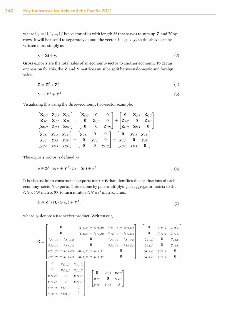
240 Key Indicators for Asia and the Pacific 2021
where
matrix Y, all vas’s into the 1 × GN vector va, and all xs’s into the GN × 1 vector x. Equation (2) may berewritten as
x = Z · iGN + Y · iG,
where iM = [1, 1, ..., 1]′ is a vector of 1’s with length M that serves to sum up Z and Y by rows. It will beuseful to separately denote the vector Y · iG as y, so the above can be written more simply as
x = Zi + y. (3)
Gross exports are the total sales of an economy–sector to another economy. To get an expression for this,the Z and Y matrices must be split between domestic and foreign sales:
Z = Zd + Zf (4)
Y = Yd + Yf (5)
Visualizing this using the three-economy, two-sector example,
ZCC ZCJ ZCU
ZJC ZJJ ZJU
ZUC ZUJ ZUU
=
ZCC 0 00 ZJJ 00 0 ZUU
+
0 ZCJ ZCU
ZJC 0 ZJU
ZUC ZUJ 0
yCC yCJ yCU
yCC yCJ yCU
yCC yCJ yCU
=
yCC 0 00 yCJ 00 0 yCU
+
0 yCJ yCU
yCC 0 yCU
yCC yCJ 0
The exports vector is defined as
e ≡ Zf · iGN + Yf · iG = Zf i + yf . (6)
It is also useful to construct an exports matrix E that identifies the destinations of each economy–sector’sexports. This is done by post-multiplying an aggregator matrix to the GN × GN matrix Zf to turn it intoa GN × G matrix. Thus,
E ≡ Zf · (IG ⊗ iN ) + Yf , (7)
3
is a vector of 1’s with length M that serves to sum up
matrix Y, all vas’s into the 1 × GN vector va, and all xs’s into the GN × 1 vector x. Equation (2) may berewritten as
x = Z · iGN + Y · iG,
where iM = [1, 1, ..., 1]′ is a vector of 1’s with length M that serves to sum up Z and Y by rows. It will beuseful to separately denote the vector Y · iG as y, so the above can be written more simply as
x = Zi + y. (3)
Gross exports are the total sales of an economy–sector to another economy. To get an expression for this,the Z and Y matrices must be split between domestic and foreign sales:
Z = Zd + Zf (4)
Y = Yd + Yf (5)
Visualizing this using the three-economy, two-sector example,
ZCC ZCJ ZCU
ZJC ZJJ ZJU
ZUC ZUJ ZUU
=
ZCC 0 00 ZJJ 00 0 ZUU
+
0 ZCJ ZCU
ZJC 0 ZJU
ZUC ZUJ 0
yCC yCJ yCU
yCC yCJ yCU
yCC yCJ yCU
=
yCC 0 00 yCJ 00 0 yCU
+
0 yCJ yCU
yCC 0 yCU
yCC yCJ 0
The exports vector is defined as
e ≡ Zf · iGN + Yf · iG = Zf i + yf . (6)
It is also useful to construct an exports matrix E that identifies the destinations of each economy–sector’sexports. This is done by post-multiplying an aggregator matrix to the GN × GN matrix Zf to turn it intoa GN × G matrix. Thus,
E ≡ Zf · (IG ⊗ iN ) + Yf , (7)
3
and
matrix Y, all vas’s into the 1 × GN vector va, and all xs’s into the GN × 1 vector x. Equation (2) may berewritten as
x = Z · iGN + Y · iG,
where iM = [1, 1, ..., 1]′ is a vector of 1’s with length M that serves to sum up Z and Y by rows. It will beuseful to separately denote the vector Y · iG as y, so the above can be written more simply as
x = Zi + y. (3)
Gross exports are the total sales of an economy–sector to another economy. To get an expression for this,the Z and Y matrices must be split between domestic and foreign sales:
Z = Zd + Zf (4)
Y = Yd + Yf (5)
Visualizing this using the three-economy, two-sector example,
ZCC ZCJ ZCU
ZJC ZJJ ZJU
ZUC ZUJ ZUU
=
ZCC 0 00 ZJJ 00 0 ZUU
+
0 ZCJ ZCU
ZJC 0 ZJU
ZUC ZUJ 0
yCC yCJ yCU
yCC yCJ yCU
yCC yCJ yCU
=
yCC 0 00 yCJ 00 0 yCU
+
0 yCJ yCU
yCC 0 yCU
yCC yCJ 0
The exports vector is defined as
e ≡ Zf · iGN + Yf · iG = Zf i + yf . (6)
It is also useful to construct an exports matrix E that identifies the destinations of each economy–sector’sexports. This is done by post-multiplying an aggregator matrix to the GN × GN matrix Zf to turn it intoa GN × G matrix. Thus,
E ≡ Zf · (IG ⊗ iN ) + Yf , (7)
3
by rows. It will be useful to separately denote the vector
matrix Y, all vas’s into the 1 × GN vector va, and all xs’s into the GN × 1 vector x. Equation (2) may berewritten as
x = Z · iGN + Y · iG,
where iM = [1, 1, ..., 1]′ is a vector of 1’s with length M that serves to sum up Z and Y by rows. It will beuseful to separately denote the vector Y · iG as y, so the above can be written more simply as
x = Zi + y. (3)
Gross exports are the total sales of an economy–sector to another economy. To get an expression for this,the Z and Y matrices must be split between domestic and foreign sales:
Z = Zd + Zf (4)
Y = Yd + Yf (5)
Visualizing this using the three-economy, two-sector example,
ZCC ZCJ ZCU
ZJC ZJJ ZJU
ZUC ZUJ ZUU
=
ZCC 0 00 ZJJ 00 0 ZUU
+
0 ZCJ ZCU
ZJC 0 ZJU
ZUC ZUJ 0
yCC yCJ yCU
yCC yCJ yCU
yCC yCJ yCU
=
yCC 0 00 yCJ 00 0 yCU
+
0 yCJ yCU
yCC 0 yCU
yCC yCJ 0
The exports vector is defined as
e ≡ Zf · iGN + Yf · iG = Zf i + yf . (6)
It is also useful to construct an exports matrix E that identifies the destinations of each economy–sector’sexports. This is done by post-multiplying an aggregator matrix to the GN × GN matrix Zf to turn it intoa GN × G matrix. Thus,
E ≡ Zf · (IG ⊗ iN ) + Yf , (7)
3
so the above can be written more simply as
matrix Y, all vas’s into the 1 × GN vector va, and all xs’s into the GN × 1 vector x. Equation (2) may berewritten as
x = Z · iGN + Y · iG,
where iM = [1, 1, ..., 1]′ is a vector of 1’s with length M that serves to sum up Z and Y by rows. It will beuseful to separately denote the vector Y · iG as y, so the above can be written more simply as
x = Zi + y. (3)
Gross exports are the total sales of an economy–sector to another economy. To get an expression for this,the Z and Y matrices must be split between domestic and foreign sales:
Z = Zd + Zf (4)
Y = Yd + Yf (5)
Visualizing this using the three-economy, two-sector example,
ZCC ZCJ ZCU
ZJC ZJJ ZJU
ZUC ZUJ ZUU
=
ZCC 0 00 ZJJ 00 0 ZUU
+
0 ZCJ ZCU
ZJC 0 ZJU
ZUC ZUJ 0
yCC yCJ yCU
yCC yCJ yCU
yCC yCJ yCU
=
yCC 0 00 yCJ 00 0 yCU
+
0 yCJ yCU
yCC 0 yCU
yCC yCJ 0
The exports vector is defined as
e ≡ Zf · iGN + Yf · iG = Zf i + yf . (6)
It is also useful to construct an exports matrix E that identifies the destinations of each economy–sector’sexports. This is done by post-multiplying an aggregator matrix to the GN × GN matrix Zf to turn it intoa GN × G matrix. Thus,
E ≡ Zf · (IG ⊗ iN ) + Yf , (7)
3
(3)
Gross exports are the total sales of an economy–sector to another economy. To get an expression for this, the
matrix Y, all vas’s into the 1 × GN vector va, and all xs’s into the GN × 1 vector x. Equation (2) may berewritten as
x = Z · iGN + Y · iG,
where iM = [1, 1, ..., 1]′ is a vector of 1’s with length M that serves to sum up Z and Y by rows. It will beuseful to separately denote the vector Y · iG as y, so the above can be written more simply as
x = Zi + y. (3)
Gross exports are the total sales of an economy–sector to another economy. To get an expression for this,the Z and Y matrices must be split between domestic and foreign sales:
Z = Zd + Zf (4)
Y = Yd + Yf (5)
Visualizing this using the three-economy, two-sector example,
ZCC ZCJ ZCU
ZJC ZJJ ZJU
ZUC ZUJ ZUU
=
ZCC 0 00 ZJJ 00 0 ZUU
+
0 ZCJ ZCU
ZJC 0 ZJU
ZUC ZUJ 0
yCC yCJ yCU
yCC yCJ yCU
yCC yCJ yCU
=
yCC 0 00 yCJ 00 0 yCU
+
0 yCJ yCU
yCC 0 yCU
yCC yCJ 0
The exports vector is defined as
e ≡ Zf · iGN + Yf · iG = Zf i + yf . (6)
It is also useful to construct an exports matrix E that identifies the destinations of each economy–sector’sexports. This is done by post-multiplying an aggregator matrix to the GN × GN matrix Zf to turn it intoa GN × G matrix. Thus,
E ≡ Zf · (IG ⊗ iN ) + Yf , (7)
3
and
matrix Y, all vas’s into the 1 × GN vector va, and all xs’s into the GN × 1 vector x. Equation (2) may berewritten as
x = Z · iGN + Y · iG,
where iM = [1, 1, ..., 1]′ is a vector of 1’s with length M that serves to sum up Z and Y by rows. It will beuseful to separately denote the vector Y · iG as y, so the above can be written more simply as
x = Zi + y. (3)
Gross exports are the total sales of an economy–sector to another economy. To get an expression for this,the Z and Y matrices must be split between domestic and foreign sales:
Z = Zd + Zf (4)
Y = Yd + Yf (5)
Visualizing this using the three-economy, two-sector example,
ZCC ZCJ ZCU
ZJC ZJJ ZJU
ZUC ZUJ ZUU
=
ZCC 0 00 ZJJ 00 0 ZUU
+
0 ZCJ ZCU
ZJC 0 ZJU
ZUC ZUJ 0
yCC yCJ yCU
yCC yCJ yCU
yCC yCJ yCU
=
yCC 0 00 yCJ 00 0 yCU
+
0 yCJ yCU
yCC 0 yCU
yCC yCJ 0
The exports vector is defined as
e ≡ Zf · iGN + Yf · iG = Zf i + yf . (6)
It is also useful to construct an exports matrix E that identifies the destinations of each economy–sector’sexports. This is done by post-multiplying an aggregator matrix to the GN × GN matrix Zf to turn it intoa GN × G matrix. Thus,
E ≡ Zf · (IG ⊗ iN ) + Yf , (7)
3
matrices must be split between domestic and foreign sales:
matrix Y, all vas’s into the 1 × GN vector va, and all xs’s into the GN × 1 vector x. Equation (2) may berewritten as
x = Z · iGN + Y · iG,
where iM = [1, 1, ..., 1]′ is a vector of 1’s with length M that serves to sum up Z and Y by rows. It will beuseful to separately denote the vector Y · iG as y, so the above can be written more simply as
x = Zi + y. (3)
Gross exports are the total sales of an economy–sector to another economy. To get an expression for this,the Z and Y matrices must be split between domestic and foreign sales:
Z = Zd + Zf (4)
Y = Yd + Yf (5)
Visualizing this using the three-economy, two-sector example,
ZCC ZCJ ZCU
ZJC ZJJ ZJU
ZUC ZUJ ZUU
=
ZCC 0 00 ZJJ 00 0 ZUU
+
0 ZCJ ZCU
ZJC 0 ZJU
ZUC ZUJ 0
yCC yCJ yCU
yCC yCJ yCU
yCC yCJ yCU
=
yCC 0 00 yCJ 00 0 yCU
+
0 yCJ yCU
yCC 0 yCU
yCC yCJ 0
The exports vector is defined as
e ≡ Zf · iGN + Yf · iG = Zf i + yf . (6)
It is also useful to construct an exports matrix E that identifies the destinations of each economy–sector’sexports. This is done by post-multiplying an aggregator matrix to the GN × GN matrix Zf to turn it intoa GN × G matrix. Thus,
E ≡ Zf · (IG ⊗ iN ) + Yf , (7)
3
(4)
matrix Y, all vas’s into the 1 × GN vector va, and all xs’s into the GN × 1 vector x. Equation (2) may berewritten as
x = Z · iGN + Y · iG,
where iM = [1, 1, ..., 1]′ is a vector of 1’s with length M that serves to sum up Z and Y by rows. It will beuseful to separately denote the vector Y · iG as y, so the above can be written more simply as
x = Zi + y. (3)
Gross exports are the total sales of an economy–sector to another economy. To get an expression for this,the Z and Y matrices must be split between domestic and foreign sales:
Z = Zd + Zf (4)
Y = Yd + Yf (5)
Visualizing this using the three-economy, two-sector example,
ZCC ZCJ ZCU
ZJC ZJJ ZJU
ZUC ZUJ ZUU
=
ZCC 0 00 ZJJ 00 0 ZUU
+
0 ZCJ ZCU
ZJC 0 ZJU
ZUC ZUJ 0
yCC yCJ yCU
yCC yCJ yCU
yCC yCJ yCU
=
yCC 0 00 yCJ 00 0 yCU
+
0 yCJ yCU
yCC 0 yCU
yCC yCJ 0
The exports vector is defined as
e ≡ Zf · iGN + Yf · iG = Zf i + yf . (6)
It is also useful to construct an exports matrix E that identifies the destinations of each economy–sector’sexports. This is done by post-multiplying an aggregator matrix to the GN × GN matrix Zf to turn it intoa GN × G matrix. Thus,
E ≡ Zf · (IG ⊗ iN ) + Yf , (7)
3
(5)
Visualizing this using the three-economy, two-sector example,
ZCC ZCJ ZCU
ZJC ZJJ ZJU
ZUC ZUJ ZUU
=
ZCC 0 00 ZJJ 00 0 ZUU
+
0 ZCJ ZCU
ZJC 0 ZJU
ZUC ZUJ 0
yCC yCJ yCU
yJC yJJ yJU
yUC yUJ yUU
=
yCC 0 00 yJJ 00 0 yUU
+
0 yCJ yCU
yJC 0 yJU
yUC yUJ 0
1
The exports vector is defined as
matrix Y, all vas’s into the 1 × GN vector va, and all xs’s into the GN × 1 vector x. Equation (2) may berewritten as
x = Z · iGN + Y · iG,
where iM = [1, 1, ..., 1]′ is a vector of 1’s with length M that serves to sum up Z and Y by rows. It will beuseful to separately denote the vector Y · iG as y, so the above can be written more simply as
x = Zi + y. (3)
Gross exports are the total sales of an economy–sector to another economy. To get an expression for this,the Z and Y matrices must be split between domestic and foreign sales:
Z = Zd + Zf (4)
Y = Yd + Yf (5)
Visualizing this using the three-economy, two-sector example,
ZCC ZCJ ZCU
ZJC ZJJ ZJU
ZUC ZUJ ZUU
=
ZCC 0 00 ZJJ 00 0 ZUU
+
0 ZCJ ZCU
ZJC 0 ZJU
ZUC ZUJ 0
yCC yCJ yCU
yCC yCJ yCU
yCC yCJ yCU
=
yCC 0 00 yCJ 00 0 yCU
+
0 yCJ yCU
yCC 0 yCU
yCC yCJ 0
The exports vector is defined as
e ≡ Zf · iGN + Yf · iG = Zf i + yf . (6)
It is also useful to construct an exports matrix E that identifies the destinations of each economy–sector’sexports. This is done by post-multiplying an aggregator matrix to the GN × GN matrix Zf to turn it intoa GN × G matrix. Thus,
E ≡ Zf · (IG ⊗ iN ) + Yf , (7)
3
(6)
It is also useful to construct an exports matrix
matrix Y, all vas’s into the 1 × GN vector va, and all xs’s into the GN × 1 vector x. Equation (2) may berewritten as
x = Z · iGN + Y · iG,
where iM = [1, 1, ..., 1]′ is a vector of 1’s with length M that serves to sum up Z and Y by rows. It will beuseful to separately denote the vector Y · iG as y, so the above can be written more simply as
x = Zi + y. (3)
Gross exports are the total sales of an economy–sector to another economy. To get an expression for this,the Z and Y matrices must be split between domestic and foreign sales:
Z = Zd + Zf (4)
Y = Yd + Yf (5)
Visualizing this using the three-economy, two-sector example,
ZCC ZCJ ZCU
ZJC ZJJ ZJU
ZUC ZUJ ZUU
=
ZCC 0 00 ZJJ 00 0 ZUU
+
0 ZCJ ZCU
ZJC 0 ZJU
ZUC ZUJ 0
yCC yCJ yCU
yCC yCJ yCU
yCC yCJ yCU
=
yCC 0 00 yCJ 00 0 yCU
+
0 yCJ yCU
yCC 0 yCU
yCC yCJ 0
The exports vector is defined as
e ≡ Zf · iGN + Yf · iG = Zf i + yf . (6)
It is also useful to construct an exports matrix E that identifies the destinations of each economy–sector’sexports. This is done by post-multiplying an aggregator matrix to the GN × GN matrix Zf to turn it intoa GN × G matrix. Thus,
E ≡ Zf · (IG ⊗ iN ) + Yf , (7)
3
that identifies the destinations of each economy–sector’s exports. This is done by post-multiplying an aggregator matrix to the
where z(s,j),(r,i) are inputs purchased by (r, i) from (s, j) and va(r,i) is (r, i) value-added. One may also callz “intermediate inputs” and va “primary inputs”. Note that variable subscripts denote flows from left toright, so that z(s,j),(r,i) means inputs are flowing from (s, j) to (r, i). An asterisk means all entities, as inz(s,j),∗ or z∗,(r,i).
Output of (r, i) is either consumed or used as inputs:
x(r,i) = z(r,i),(1,1) + z(r,i),(1,2) + ... + z(r,i),(u,i) + ... + z(r,i),(G,N)+
y(r,i),1 + ... + y(r,i),u + ... + y(r,i),G, (2)
where y(r,i),u are (r, i) output consumed in economy u. Market clearing is assumed to always hold, soequations (1) and (2) are equal.
These relationships are more neatly presented in a table. For the case of three economies {C, J, U} and twosectors {1, 2}, the full table is as follows:
Buying economiesTotalsales
Intermediate sales Final salesC J U
C J U1 2 1 2 1 2
Sellingeconomies
C1 zC1,C1 zC1,C2 zC1,J1 zC1,J2 zC1,U1 zC1,U2 yC1,C yC1,J yC1,U xC1
2 zC2,C1 zC2,C2 zC2,J1 zC2,J2 zC2,U1 zC2,U2 yC2,C yC2,J yC2,U xC2
J1 zJ1,C1 zJ1,C2 zJ1,J1 zJ1,J2 zJ1,U1 zJ1,U2 yJ1,C yJ1,J yJ1,U xJ1
2 zJ2,C1 zJ2,C2 zJ2,J1 zJ2,J2 zJ2,U1 zJ2,U2 yJ2,C yJ2,J yJ2,U xJ2
U1 zU1,C1 zU1,C2 zU1,J1 zU1,J2 zU1,U1 zU1,U2 yU1,C yU1,J yU1,U xU1
2 zU2,C1 zU2,C2 zU2,J1 zU2,J2 zU2,U1 zU2,U2 yU2,C yU2,J yU2,U xU2
Value-added vaC1 vaC2 vaJ1 vaJ2 vaU1 vaU2
Total outlays xC1 xC2 xJ1 xJ2 xU1 xU2
The GN equations of (1) are arranged in columns while the GN equations of (2) are arranged in rows. It isclear that for larger G and N , representation in table form becomes unwieldy. One fix would be to collecteconomy-specific terms into matrices and vectors:
Buying economiesTotal salesIntermediate sales Final sales
C J U C J U
Selling economiesC ZCC ZCJ ZCU yCC yCJ yCU xC
J ZJC ZJJ ZJU yJC yJJ yJU xJ
U ZUC ZUJ ZUU yUC yUJ yUU xU
Value-added vaC vaJ vaU
Total outlays x′C x′
J x′U
Uppercase letters in bold denote matrices while lowercase letters in bold denote vectors. These may furtherbe collected into larger matrices and vectors: all Zsr’s into the GN ×GN matrix Z, all ysr’s into the GN ×G
2
matrix
matrix Y, all vas’s into the 1 × GN vector va, and all xs’s into the GN × 1 vector x. Equation (2) may berewritten as
x = Z · iGN + Y · iG,
where iM = [1, 1, ..., 1]′ is a vector of 1’s with length M that serves to sum up Z and Y by rows. It will beuseful to separately denote the vector Y · iG as y, so the above can be written more simply as
x = Zi + y. (3)
Gross exports are the total sales of an economy–sector to another economy. To get an expression for this,the Z and Y matrices must be split between domestic and foreign sales:
Z = Zd + Zf (4)
Y = Yd + Yf (5)
Visualizing this using the three-economy, two-sector example,
ZCC ZCJ ZCU
ZJC ZJJ ZJU
ZUC ZUJ ZUU
=
ZCC 0 00 ZJJ 00 0 ZUU
+
0 ZCJ ZCU
ZJC 0 ZJU
ZUC ZUJ 0
yCC yCJ yCU
yCC yCJ yCU
yCC yCJ yCU
=
yCC 0 00 yCJ 00 0 yCU
+
0 yCJ yCU
yCC 0 yCU
yCC yCJ 0
The exports vector is defined as
e ≡ Zf · iGN + Yf · iG = Zf i + yf . (6)
It is also useful to construct an exports matrix E that identifies the destinations of each economy–sector’sexports. This is done by post-multiplying an aggregator matrix to the GN × GN matrix Zf to turn it intoa GN × G matrix. Thus,
E ≡ Zf · (IG ⊗ iN ) + Yf , (7)
3
to turn it into a
where z(s,j),(r,i) are inputs purchased by (r, i) from (s, j) and va(r,i) is (r, i) value-added. One may also callz “intermediate inputs” and va “primary inputs”. Note that variable subscripts denote flows from left toright, so that z(s,j),(r,i) means inputs are flowing from (s, j) to (r, i). An asterisk means all entities, as inz(s,j),∗ or z∗,(r,i).
Output of (r, i) is either consumed or used as inputs:
x(r,i) = z(r,i),(1,1) + z(r,i),(1,2) + ... + z(r,i),(u,i) + ... + z(r,i),(G,N)+
y(r,i),1 + ... + y(r,i),u + ... + y(r,i),G, (2)
where y(r,i),u are (r, i) output consumed in economy u. Market clearing is assumed to always hold, soequations (1) and (2) are equal.
These relationships are more neatly presented in a table. For the case of three economies {C, J, U} and twosectors {1, 2}, the full table is as follows:
Buying economiesTotalsales
Intermediate sales Final salesC J U
C J U1 2 1 2 1 2
Sellingeconomies
C1 zC1,C1 zC1,C2 zC1,J1 zC1,J2 zC1,U1 zC1,U2 yC1,C yC1,J yC1,U xC1
2 zC2,C1 zC2,C2 zC2,J1 zC2,J2 zC2,U1 zC2,U2 yC2,C yC2,J yC2,U xC2
J1 zJ1,C1 zJ1,C2 zJ1,J1 zJ1,J2 zJ1,U1 zJ1,U2 yJ1,C yJ1,J yJ1,U xJ1
2 zJ2,C1 zJ2,C2 zJ2,J1 zJ2,J2 zJ2,U1 zJ2,U2 yJ2,C yJ2,J yJ2,U xJ2
U1 zU1,C1 zU1,C2 zU1,J1 zU1,J2 zU1,U1 zU1,U2 yU1,C yU1,J yU1,U xU1
2 zU2,C1 zU2,C2 zU2,J1 zU2,J2 zU2,U1 zU2,U2 yU2,C yU2,J yU2,U xU2
Value-added vaC1 vaC2 vaJ1 vaJ2 vaU1 vaU2
Total outlays xC1 xC2 xJ1 xJ2 xU1 xU2
The GN equations of (1) are arranged in columns while the GN equations of (2) are arranged in rows. It isclear that for larger G and N , representation in table form becomes unwieldy. One fix would be to collecteconomy-specific terms into matrices and vectors:
Buying economiesTotal salesIntermediate sales Final sales
C J U C J U
Selling economiesC ZCC ZCJ ZCU yCC yCJ yCU xC
J ZJC ZJJ ZJU yJC yJJ yJU xJ
U ZUC ZUJ ZUU yUC yUJ yUU xU
Value-added vaC vaJ vaU
Total outlays x′C x′
J x′U
Uppercase letters in bold denote matrices while lowercase letters in bold denote vectors. These may furtherbe collected into larger matrices and vectors: all Zsr’s into the GN ×GN matrix Z, all ysr’s into the GN ×G
2
matrix. Thus,
matrix Y, all vas’s into the 1 × GN vector va, and all xs’s into the GN × 1 vector x. Equation (2) may berewritten as
x = Z · iGN + Y · iG,
where iM = [1, 1, ..., 1]′ is a vector of 1’s with length M that serves to sum up Z and Y by rows. It will beuseful to separately denote the vector Y · iG as y, so the above can be written more simply as
x = Zi + y. (3)
Gross exports are the total sales of an economy–sector to another economy. To get an expression for this,the Z and Y matrices must be split between domestic and foreign sales:
Z = Zd + Zf (4)
Y = Yd + Yf (5)
Visualizing this using the three-economy, two-sector example,
ZCC ZCJ ZCU
ZJC ZJJ ZJU
ZUC ZUJ ZUU
=
ZCC 0 00 ZJJ 00 0 ZUU
+
0 ZCJ ZCU
ZJC 0 ZJU
ZUC ZUJ 0
yCC yCJ yCU
yCC yCJ yCU
yCC yCJ yCU
=
yCC 0 00 yCJ 00 0 yCU
+
0 yCJ yCU
yCC 0 yCU
yCC yCJ 0
The exports vector is defined as
e ≡ Zf · iGN + Yf · iG = Zf i + yf . (6)
It is also useful to construct an exports matrix E that identifies the destinations of each economy–sector’sexports. This is done by post-multiplying an aggregator matrix to the GN × GN matrix Zf to turn it intoa GN × G matrix. Thus,
E ≡ Zf · (IG ⊗ iN ) + Yf , (7)
3
(7)
where where ⊗ denote a Kronecker product. Written out,
E ≡
0 zC1,J1 + zC1,J2 zC1,U1 + zC1,U2
0 zC2,J1 + zC2,J2 zC2,U1 + zC2,U2
zJ1,C1 + zJ1,C2 0 zJ1,U1 + zJ1,U2
zJ2,C1 + zJ2,C2 0 zJ2,U1 + zJ2,U2
zU1,C1 + zU1,C2 zU1,J1 + zU1,J2 0zU2,C1 + zU2,C2 zU2,J1 + zU2,J2 0
+
0 yC1,J yC1,U
0 yC2,J yC2,U
yJ1,C 0 yJ1,U
yJ2,C 0 yJ2,U
yU1,C yU1,J 0yU2,C yU2,J 0
=
0 eC1,J eC1,U
0 eC2,J eC2,U
eJ1,C 0 eJ1,U
eJ2,C 0 eJ2,U
eU1,C eU1,J 0eU2,C eU2,J 0
=
0 eCJ eCU
eJC 0 eJU
eUC eUJ 0
The technical coefficient a(s,j),(r,i) is the share of inputs from (s, j) in the output of (r, i): a(s,j),(r,i) ≡z(s,j),(r,i)/x(r,i). Collect all these into the GN × GN matrix of technical coefficients A. This may be used torewrite (3) as
x = Ax + y. (8)
Solving for x gives
x = (I − A)−1y = By, (9)
where the GN × GN matrix B is called the global Leontief inverse matrix.
VB Decomposition
Equation (9) is central to analyzing cross-economy and cross-sectoral linkages. It is clearer to see this if (8)and (9) are rewritten to isolate a single economy s:
xs =Gr
Asrxr +Gr
ysr (10)
=Gr
Gu
Bsryru (11)
Equation (10) says that s’s output xs is used as intermediates in r’s output or sold as final goods to r (for allr = 1, ..., G). The output of each r can in turn be used as intermediates by other economies, whose outputsare then used by further economies, and so on in a potentially infinite series of production stages. Equation(11) summarizes these to identify the final landing stage of s’s output. The product Bsryru is s output thatis “completed” into a final good by r, which then sends it to u for final absorption.
In most analyses, value-added rather than output is the preferred metric. Define the vector v with (s, i)th
4
denote a Kronecker product. Written out,
where ⊗ denote a Kronecker product. Written out,
E ≡
0 zC1,J1 + zC1,J2 zC1,U1 + zC1,U2
0 zC2,J1 + zC2,J2 zC2,U1 + zC2,U2
zJ1,C1 + zJ1,C2 0 zJ1,U1 + zJ1,U2
zJ2,C1 + zJ2,C2 0 zJ2,U1 + zJ2,U2
zU1,C1 + zU1,C2 zU1,J1 + zU1,J2 0zU2,C1 + zU2,C2 zU2,J1 + zU2,J2 0
+
0 yC1,J yC1,U
0 yC2,J yC2,U
yJ1,C 0 yJ1,U
yJ2,C 0 yJ2,U
yU1,C yU1,J 0yU2,C yU2,J 0
=
0 eC1,J eC1,U
0 eC2,J eC2,U
eJ1,C 0 eJ1,U
eJ2,C 0 eJ2,U
eU1,C eU1,J 0eU2,C eU2,J 0
=
0 eCJ eCU
eJC 0 eJU
eUC eUJ 0
The technical coefficient a(s,j),(r,i) is the share of inputs from (s, j) in the output of (r, i): a(s,j),(r,i) ≡z(s,j),(r,i)/x(r,i). Collect all these into the GN × GN matrix of technical coefficients A. This may be used torewrite (3) as
x = Ax + y. (8)
Solving for x gives
x = (I − A)−1y = By, (9)
where the GN × GN matrix B is called the global Leontief inverse matrix.
VB Decomposition
Equation (9) is central to analyzing cross-economy and cross-sectoral linkages. It is clearer to see this if (8)and (9) are rewritten to isolate a single economy s:
xs =Gr
Asrxr +Gr
ysr (10)
=Gr
Gu
Bsryru (11)
Equation (10) says that s’s output xs is used as intermediates in r’s output or sold as final goods to r (for allr = 1, ..., G). The output of each r can in turn be used as intermediates by other economies, whose outputsare then used by further economies, and so on in a potentially infinite series of production stages. Equation(11) summarizes these to identify the final landing stage of s’s output. The product Bsryru is s output thatis “completed” into a final good by r, which then sends it to u for final absorption.
In most analyses, value-added rather than output is the preferred metric. Define the vector v with (s, i)th
4
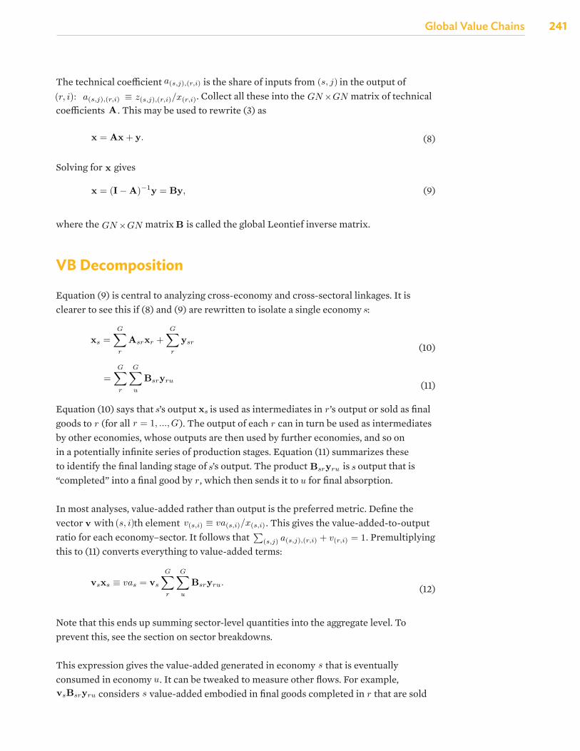
Global Value Chains
241Global Value Chains
The technical coefficient
where ⊗ denote a Kronecker product. Written out,
E ≡
0 zC1,J1 + zC1,J2 zC1,U1 + zC1,U2
0 zC2,J1 + zC2,J2 zC2,U1 + zC2,U2
zJ1,C1 + zJ1,C2 0 zJ1,U1 + zJ1,U2
zJ2,C1 + zJ2,C2 0 zJ2,U1 + zJ2,U2
zU1,C1 + zU1,C2 zU1,J1 + zU1,J2 0zU2,C1 + zU2,C2 zU2,J1 + zU2,J2 0
+
0 yC1,J yC1,U
0 yC2,J yC2,U
yJ1,C 0 yJ1,U
yJ2,C 0 yJ2,U
yU1,C yU1,J 0yU2,C yU2,J 0
=
0 eC1,J eC1,U
0 eC2,J eC2,U
eJ1,C 0 eJ1,U
eJ2,C 0 eJ2,U
eU1,C eU1,J 0eU2,C eU2,J 0
=
0 eCJ eCU
eJC 0 eJU
eUC eUJ 0
The technical coefficient a(s,j),(r,i) is the share of inputs from (s, j) in the output of (r, i): a(s,j),(r,i) ≡z(s,j),(r,i)/x(r,i). Collect all these into the GN × GN matrix of technical coefficients A. This may be used torewrite (3) as
x = Ax + y. (8)
Solving for x gives
x = (I − A)−1y = By, (9)
where the GN × GN matrix B is called the global Leontief inverse matrix.
VB Decomposition
Equation (9) is central to analyzing cross-economy and cross-sectoral linkages. It is clearer to see this if (8)and (9) are rewritten to isolate a single economy s:
xs =Gr
Asrxr +Gr
ysr (10)
=Gr
Gu
Bsryru (11)
Equation (10) says that s’s output xs is used as intermediates in r’s output or sold as final goods to r (for allr = 1, ..., G). The output of each r can in turn be used as intermediates by other economies, whose outputsare then used by further economies, and so on in a potentially infinite series of production stages. Equation(11) summarizes these to identify the final landing stage of s’s output. The product Bsryru is s output thatis “completed” into a final good by r, which then sends it to u for final absorption.
In most analyses, value-added rather than output is the preferred metric. Define the vector v with (s, i)th
4
is the share of inputs from where z(s,j),(r,i) are inputs purchased by (r, i) from (s, j) and va(r,i) is (r, i) value-added. One may also callz “intermediate inputs” and va “primary inputs”. Note that variable subscripts denote flows from left toright, so that z(s,j),(r,i) means inputs are flowing from (s, j) to (r, i). An asterisk means all entities, as inz(s,j),∗ or z∗,(r,i).
Output of (r, i) is either consumed or used as inputs:
x(r,i) = z(r,i),(1,1) + z(r,i),(1,2) + ... + z(r,i),(u,i) + ... + z(r,i),(G,N)+
y(r,i),1 + ... + y(r,i),u + ... + y(r,i),G, (2)
where y(r,i),u are (r, i) output consumed in economy u. Market clearing is assumed to always hold, soequations (1) and (2) are equal.
These relationships are more neatly presented in a table. For the case of three economies {C, J, U} and twosectors {1, 2}, the full table is as follows:
Buying economiesTotalsales
Intermediate sales Final salesC J U
C J U1 2 1 2 1 2
Sellingeconomies
C1 zC1,C1 zC1,C2 zC1,J1 zC1,J2 zC1,U1 zC1,U2 yC1,C yC1,J yC1,U xC1
2 zC2,C1 zC2,C2 zC2,J1 zC2,J2 zC2,U1 zC2,U2 yC2,C yC2,J yC2,U xC2
J1 zJ1,C1 zJ1,C2 zJ1,J1 zJ1,J2 zJ1,U1 zJ1,U2 yJ1,C yJ1,J yJ1,U xJ1
2 zJ2,C1 zJ2,C2 zJ2,J1 zJ2,J2 zJ2,U1 zJ2,U2 yJ2,C yJ2,J yJ2,U xJ2
U1 zU1,C1 zU1,C2 zU1,J1 zU1,J2 zU1,U1 zU1,U2 yU1,C yU1,J yU1,U xU1
2 zU2,C1 zU2,C2 zU2,J1 zU2,J2 zU2,U1 zU2,U2 yU2,C yU2,J yU2,U xU2
Value-added vaC1 vaC2 vaJ1 vaJ2 vaU1 vaU2
Total outlays xC1 xC2 xJ1 xJ2 xU1 xU2
The GN equations of (1) are arranged in columns while the GN equations of (2) are arranged in rows. It isclear that for larger G and N , representation in table form becomes unwieldy. One fix would be to collecteconomy-specific terms into matrices and vectors:
Buying economiesTotal salesIntermediate sales Final sales
C J U C J U
Selling economiesC ZCC ZCJ ZCU yCC yCJ yCU xC
J ZJC ZJJ ZJU yJC yJJ yJU xJ
U ZUC ZUJ ZUU yUC yUJ yUU xU
Value-added vaC vaJ vaU
Total outlays x′C x′
J x′U
Uppercase letters in bold denote matrices while lowercase letters in bold denote vectors. These may furtherbe collected into larger matrices and vectors: all Zsr’s into the GN ×GN matrix Z, all ysr’s into the GN ×G
2
in the output of
where ⊗ denote a Kronecker product. Written out,
E ≡
0 zC1,J1 + zC1,J2 zC1,U1 + zC1,U2
0 zC2,J1 + zC2,J2 zC2,U1 + zC2,U2
zJ1,C1 + zJ1,C2 0 zJ1,U1 + zJ1,U2
zJ2,C1 + zJ2,C2 0 zJ2,U1 + zJ2,U2
zU1,C1 + zU1,C2 zU1,J1 + zU1,J2 0zU2,C1 + zU2,C2 zU2,J1 + zU2,J2 0
+
0 yC1,J yC1,U
0 yC2,J yC2,U
yJ1,C 0 yJ1,U
yJ2,C 0 yJ2,U
yU1,C yU1,J 0yU2,C yU2,J 0
=
0 eC1,J eC1,U
0 eC2,J eC2,U
eJ1,C 0 eJ1,U
eJ2,C 0 eJ2,U
eU1,C eU1,J 0eU2,C eU2,J 0
=
0 eCJ eCU
eJC 0 eJU
eUC eUJ 0
The technical coefficient a(s,j),(r,i) is the share of inputs from (s, j) in the output of (r, i): a(s,j),(r,i) ≡z(s,j),(r,i)/x(r,i). Collect all these into the GN × GN matrix of technical coefficients A. This may be used torewrite (3) as
x = Ax + y. (8)
Solving for x gives
x = (I − A)−1y = By, (9)
where the GN × GN matrix B is called the global Leontief inverse matrix.
VB Decomposition
Equation (9) is central to analyzing cross-economy and cross-sectoral linkages. It is clearer to see this if (8)and (9) are rewritten to isolate a single economy s:
xs =Gr
Asrxr +Gr
ysr (10)
=Gr
Gu
Bsryru (11)
Equation (10) says that s’s output xs is used as intermediates in r’s output or sold as final goods to r (for allr = 1, ..., G). The output of each r can in turn be used as intermediates by other economies, whose outputsare then used by further economies, and so on in a potentially infinite series of production stages. Equation(11) summarizes these to identify the final landing stage of s’s output. The product Bsryru is s output thatis “completed” into a final good by r, which then sends it to u for final absorption.
In most analyses, value-added rather than output is the preferred metric. Define the vector v with (s, i)th
4
. Collect all these into the
where z(s,j),(r,i) are inputs purchased by (r, i) from (s, j) and va(r,i) is (r, i) value-added. One may also callz “intermediate inputs” and va “primary inputs”. Note that variable subscripts denote flows from left toright, so that z(s,j),(r,i) means inputs are flowing from (s, j) to (r, i). An asterisk means all entities, as inz(s,j),∗ or z∗,(r,i).
Output of (r, i) is either consumed or used as inputs:
x(r,i) = z(r,i),(1,1) + z(r,i),(1,2) + ... + z(r,i),(u,i) + ... + z(r,i),(G,N)+
y(r,i),1 + ... + y(r,i),u + ... + y(r,i),G, (2)
where y(r,i),u are (r, i) output consumed in economy u. Market clearing is assumed to always hold, soequations (1) and (2) are equal.
These relationships are more neatly presented in a table. For the case of three economies {C, J, U} and twosectors {1, 2}, the full table is as follows:
Buying economiesTotalsales
Intermediate sales Final salesC J U
C J U1 2 1 2 1 2
Sellingeconomies
C1 zC1,C1 zC1,C2 zC1,J1 zC1,J2 zC1,U1 zC1,U2 yC1,C yC1,J yC1,U xC1
2 zC2,C1 zC2,C2 zC2,J1 zC2,J2 zC2,U1 zC2,U2 yC2,C yC2,J yC2,U xC2
J1 zJ1,C1 zJ1,C2 zJ1,J1 zJ1,J2 zJ1,U1 zJ1,U2 yJ1,C yJ1,J yJ1,U xJ1
2 zJ2,C1 zJ2,C2 zJ2,J1 zJ2,J2 zJ2,U1 zJ2,U2 yJ2,C yJ2,J yJ2,U xJ2
U1 zU1,C1 zU1,C2 zU1,J1 zU1,J2 zU1,U1 zU1,U2 yU1,C yU1,J yU1,U xU1
2 zU2,C1 zU2,C2 zU2,J1 zU2,J2 zU2,U1 zU2,U2 yU2,C yU2,J yU2,U xU2
Value-added vaC1 vaC2 vaJ1 vaJ2 vaU1 vaU2
Total outlays xC1 xC2 xJ1 xJ2 xU1 xU2
The GN equations of (1) are arranged in columns while the GN equations of (2) are arranged in rows. It isclear that for larger G and N , representation in table form becomes unwieldy. One fix would be to collecteconomy-specific terms into matrices and vectors:
Buying economiesTotal salesIntermediate sales Final sales
C J U C J U
Selling economiesC ZCC ZCJ ZCU yCC yCJ yCU xC
J ZJC ZJJ ZJU yJC yJJ yJU xJ
U ZUC ZUJ ZUU yUC yUJ yUU xU
Value-added vaC vaJ vaU
Total outlays x′C x′
J x′U
Uppercase letters in bold denote matrices while lowercase letters in bold denote vectors. These may furtherbe collected into larger matrices and vectors: all Zsr’s into the GN ×GN matrix Z, all ysr’s into the GN ×G
2
matrix of technical coefficients
where ⊗ denote a Kronecker product. Written out,
E ≡
0 zC1,J1 + zC1,J2 zC1,U1 + zC1,U2
0 zC2,J1 + zC2,J2 zC2,U1 + zC2,U2
zJ1,C1 + zJ1,C2 0 zJ1,U1 + zJ1,U2
zJ2,C1 + zJ2,C2 0 zJ2,U1 + zJ2,U2
zU1,C1 + zU1,C2 zU1,J1 + zU1,J2 0zU2,C1 + zU2,C2 zU2,J1 + zU2,J2 0
+
0 yC1,J yC1,U
0 yC2,J yC2,U
yJ1,C 0 yJ1,U
yJ2,C 0 yJ2,U
yU1,C yU1,J 0yU2,C yU2,J 0
=
0 eC1,J eC1,U
0 eC2,J eC2,U
eJ1,C 0 eJ1,U
eJ2,C 0 eJ2,U
eU1,C eU1,J 0eU2,C eU2,J 0
=
0 eCJ eCU
eJC 0 eJU
eUC eUJ 0
The technical coefficient a(s,j),(r,i) is the share of inputs from (s, j) in the output of (r, i): a(s,j),(r,i) ≡z(s,j),(r,i)/x(r,i). Collect all these into the GN × GN matrix of technical coefficients A. This may be used torewrite (3) as
x = Ax + y. (8)
Solving for x gives
x = (I − A)−1y = By, (9)
where the GN × GN matrix B is called the global Leontief inverse matrix.
VB Decomposition
Equation (9) is central to analyzing cross-economy and cross-sectoral linkages. It is clearer to see this if (8)and (9) are rewritten to isolate a single economy s:
xs =Gr
Asrxr +Gr
ysr (10)
=Gr
Gu
Bsryru (11)
Equation (10) says that s’s output xs is used as intermediates in r’s output or sold as final goods to r (for allr = 1, ..., G). The output of each r can in turn be used as intermediates by other economies, whose outputsare then used by further economies, and so on in a potentially infinite series of production stages. Equation(11) summarizes these to identify the final landing stage of s’s output. The product Bsryru is s output thatis “completed” into a final good by r, which then sends it to u for final absorption.
In most analyses, value-added rather than output is the preferred metric. Define the vector v with (s, i)th
4
. This may be used to rewrite (3) as
where ⊗ denote a Kronecker product. Written out,
E ≡
0 zC1,J1 + zC1,J2 zC1,U1 + zC1,U2
0 zC2,J1 + zC2,J2 zC2,U1 + zC2,U2
zJ1,C1 + zJ1,C2 0 zJ1,U1 + zJ1,U2
zJ2,C1 + zJ2,C2 0 zJ2,U1 + zJ2,U2
zU1,C1 + zU1,C2 zU1,J1 + zU1,J2 0zU2,C1 + zU2,C2 zU2,J1 + zU2,J2 0
+
0 yC1,J yC1,U
0 yC2,J yC2,U
yJ1,C 0 yJ1,U
yJ2,C 0 yJ2,U
yU1,C yU1,J 0yU2,C yU2,J 0
=
0 eC1,J eC1,U
0 eC2,J eC2,U
eJ1,C 0 eJ1,U
eJ2,C 0 eJ2,U
eU1,C eU1,J 0eU2,C eU2,J 0
=
0 eCJ eCU
eJC 0 eJU
eUC eUJ 0
The technical coefficient a(s,j),(r,i) is the share of inputs from (s, j) in the output of (r, i): a(s,j),(r,i) ≡z(s,j),(r,i)/x(r,i). Collect all these into the GN × GN matrix of technical coefficients A. This may be used torewrite (3) as
x = Ax + y. (8)
Solving for x gives
x = (I − A)−1y = By, (9)
where the GN × GN matrix B is called the global Leontief inverse matrix.
VB Decomposition
Equation (9) is central to analyzing cross-economy and cross-sectoral linkages. It is clearer to see this if (8)and (9) are rewritten to isolate a single economy s:
xs =Gr
Asrxr +Gr
ysr (10)
=Gr
Gu
Bsryru (11)
Equation (10) says that s’s output xs is used as intermediates in r’s output or sold as final goods to r (for allr = 1, ..., G). The output of each r can in turn be used as intermediates by other economies, whose outputsare then used by further economies, and so on in a potentially infinite series of production stages. Equation(11) summarizes these to identify the final landing stage of s’s output. The product Bsryru is s output thatis “completed” into a final good by r, which then sends it to u for final absorption.
In most analyses, value-added rather than output is the preferred metric. Define the vector v with (s, i)th
4
(8)
Solving for
where ⊗ denote a Kronecker product. Written out,
E ≡
0 zC1,J1 + zC1,J2 zC1,U1 + zC1,U2
0 zC2,J1 + zC2,J2 zC2,U1 + zC2,U2
zJ1,C1 + zJ1,C2 0 zJ1,U1 + zJ1,U2
zJ2,C1 + zJ2,C2 0 zJ2,U1 + zJ2,U2
zU1,C1 + zU1,C2 zU1,J1 + zU1,J2 0zU2,C1 + zU2,C2 zU2,J1 + zU2,J2 0
+
0 yC1,J yC1,U
0 yC2,J yC2,U
yJ1,C 0 yJ1,U
yJ2,C 0 yJ2,U
yU1,C yU1,J 0yU2,C yU2,J 0
=
0 eC1,J eC1,U
0 eC2,J eC2,U
eJ1,C 0 eJ1,U
eJ2,C 0 eJ2,U
eU1,C eU1,J 0eU2,C eU2,J 0
=
0 eCJ eCU
eJC 0 eJU
eUC eUJ 0
The technical coefficient a(s,j),(r,i) is the share of inputs from (s, j) in the output of (r, i): a(s,j),(r,i) ≡z(s,j),(r,i)/x(r,i). Collect all these into the GN × GN matrix of technical coefficients A. This may be used torewrite (3) as
x = Ax + y. (8)
Solving for x gives
x = (I − A)−1y = By, (9)
where the GN × GN matrix B is called the global Leontief inverse matrix.
VB Decomposition
Equation (9) is central to analyzing cross-economy and cross-sectoral linkages. It is clearer to see this if (8)and (9) are rewritten to isolate a single economy s:
xs =Gr
Asrxr +Gr
ysr (10)
=Gr
Gu
Bsryru (11)
Equation (10) says that s’s output xs is used as intermediates in r’s output or sold as final goods to r (for allr = 1, ..., G). The output of each r can in turn be used as intermediates by other economies, whose outputsare then used by further economies, and so on in a potentially infinite series of production stages. Equation(11) summarizes these to identify the final landing stage of s’s output. The product Bsryru is s output thatis “completed” into a final good by r, which then sends it to u for final absorption.
In most analyses, value-added rather than output is the preferred metric. Define the vector v with (s, i)th
4
gives
where ⊗ denote a Kronecker product. Written out,
E ≡
0 zC1,J1 + zC1,J2 zC1,U1 + zC1,U2
0 zC2,J1 + zC2,J2 zC2,U1 + zC2,U2
zJ1,C1 + zJ1,C2 0 zJ1,U1 + zJ1,U2
zJ2,C1 + zJ2,C2 0 zJ2,U1 + zJ2,U2
zU1,C1 + zU1,C2 zU1,J1 + zU1,J2 0zU2,C1 + zU2,C2 zU2,J1 + zU2,J2 0
+
0 yC1,J yC1,U
0 yC2,J yC2,U
yJ1,C 0 yJ1,U
yJ2,C 0 yJ2,U
yU1,C yU1,J 0yU2,C yU2,J 0
=
0 eC1,J eC1,U
0 eC2,J eC2,U
eJ1,C 0 eJ1,U
eJ2,C 0 eJ2,U
eU1,C eU1,J 0eU2,C eU2,J 0
=
0 eCJ eCU
eJC 0 eJU
eUC eUJ 0
The technical coefficient a(s,j),(r,i) is the share of inputs from (s, j) in the output of (r, i): a(s,j),(r,i) ≡z(s,j),(r,i)/x(r,i). Collect all these into the GN × GN matrix of technical coefficients A. This may be used torewrite (3) as
x = Ax + y. (8)
Solving for x gives
x = (I − A)−1y = By, (9)
where the GN × GN matrix B is called the global Leontief inverse matrix.
VB Decomposition
Equation (9) is central to analyzing cross-economy and cross-sectoral linkages. It is clearer to see this if (8)and (9) are rewritten to isolate a single economy s:
xs =Gr
Asrxr +Gr
ysr (10)
=Gr
Gu
Bsryru (11)
Equation (10) says that s’s output xs is used as intermediates in r’s output or sold as final goods to r (for allr = 1, ..., G). The output of each r can in turn be used as intermediates by other economies, whose outputsare then used by further economies, and so on in a potentially infinite series of production stages. Equation(11) summarizes these to identify the final landing stage of s’s output. The product Bsryru is s output thatis “completed” into a final good by r, which then sends it to u for final absorption.
In most analyses, value-added rather than output is the preferred metric. Define the vector v with (s, i)th
4
(9)
where the
where z(s,j),(r,i) are inputs purchased by (r, i) from (s, j) and va(r,i) is (r, i) value-added. One may also callz “intermediate inputs” and va “primary inputs”. Note that variable subscripts denote flows from left toright, so that z(s,j),(r,i) means inputs are flowing from (s, j) to (r, i). An asterisk means all entities, as inz(s,j),∗ or z∗,(r,i).
Output of (r, i) is either consumed or used as inputs:
x(r,i) = z(r,i),(1,1) + z(r,i),(1,2) + ... + z(r,i),(u,i) + ... + z(r,i),(G,N)+
y(r,i),1 + ... + y(r,i),u + ... + y(r,i),G, (2)
where y(r,i),u are (r, i) output consumed in economy u. Market clearing is assumed to always hold, soequations (1) and (2) are equal.
These relationships are more neatly presented in a table. For the case of three economies {C, J, U} and twosectors {1, 2}, the full table is as follows:
Buying economiesTotalsales
Intermediate sales Final salesC J U
C J U1 2 1 2 1 2
Sellingeconomies
C1 zC1,C1 zC1,C2 zC1,J1 zC1,J2 zC1,U1 zC1,U2 yC1,C yC1,J yC1,U xC1
2 zC2,C1 zC2,C2 zC2,J1 zC2,J2 zC2,U1 zC2,U2 yC2,C yC2,J yC2,U xC2
J1 zJ1,C1 zJ1,C2 zJ1,J1 zJ1,J2 zJ1,U1 zJ1,U2 yJ1,C yJ1,J yJ1,U xJ1
2 zJ2,C1 zJ2,C2 zJ2,J1 zJ2,J2 zJ2,U1 zJ2,U2 yJ2,C yJ2,J yJ2,U xJ2
U1 zU1,C1 zU1,C2 zU1,J1 zU1,J2 zU1,U1 zU1,U2 yU1,C yU1,J yU1,U xU1
2 zU2,C1 zU2,C2 zU2,J1 zU2,J2 zU2,U1 zU2,U2 yU2,C yU2,J yU2,U xU2
Value-added vaC1 vaC2 vaJ1 vaJ2 vaU1 vaU2
Total outlays xC1 xC2 xJ1 xJ2 xU1 xU2
The GN equations of (1) are arranged in columns while the GN equations of (2) are arranged in rows. It isclear that for larger G and N , representation in table form becomes unwieldy. One fix would be to collecteconomy-specific terms into matrices and vectors:
Buying economiesTotal salesIntermediate sales Final sales
C J U C J U
Selling economiesC ZCC ZCJ ZCU yCC yCJ yCU xC
J ZJC ZJJ ZJU yJC yJJ yJU xJ
U ZUC ZUJ ZUU yUC yUJ yUU xU
Value-added vaC vaJ vaU
Total outlays x′C x′
J x′U
Uppercase letters in bold denote matrices while lowercase letters in bold denote vectors. These may furtherbe collected into larger matrices and vectors: all Zsr’s into the GN ×GN matrix Z, all ysr’s into the GN ×G
2
matrix
where ⊗ denote a Kronecker product. Written out,
E ≡
0 zC1,J1 + zC1,J2 zC1,U1 + zC1,U2
0 zC2,J1 + zC2,J2 zC2,U1 + zC2,U2
zJ1,C1 + zJ1,C2 0 zJ1,U1 + zJ1,U2
zJ2,C1 + zJ2,C2 0 zJ2,U1 + zJ2,U2
zU1,C1 + zU1,C2 zU1,J1 + zU1,J2 0zU2,C1 + zU2,C2 zU2,J1 + zU2,J2 0
+
0 yC1,J yC1,U
0 yC2,J yC2,U
yJ1,C 0 yJ1,U
yJ2,C 0 yJ2,U
yU1,C yU1,J 0yU2,C yU2,J 0
=
0 eC1,J eC1,U
0 eC2,J eC2,U
eJ1,C 0 eJ1,U
eJ2,C 0 eJ2,U
eU1,C eU1,J 0eU2,C eU2,J 0
=
0 eCJ eCU
eJC 0 eJU
eUC eUJ 0
The technical coefficient a(s,j),(r,i) is the share of inputs from (s, j) in the output of (r, i): a(s,j),(r,i) ≡z(s,j),(r,i)/x(r,i). Collect all these into the GN × GN matrix of technical coefficients A. This may be used torewrite (3) as
x = Ax + y. (8)
Solving for x gives
x = (I − A)−1y = By, (9)
where the GN × GN matrix B is called the global Leontief inverse matrix.
VB Decomposition
Equation (9) is central to analyzing cross-economy and cross-sectoral linkages. It is clearer to see this if (8)and (9) are rewritten to isolate a single economy s:
xs =Gr
Asrxr +Gr
ysr (10)
=Gr
Gu
Bsryru (11)
Equation (10) says that s’s output xs is used as intermediates in r’s output or sold as final goods to r (for allr = 1, ..., G). The output of each r can in turn be used as intermediates by other economies, whose outputsare then used by further economies, and so on in a potentially infinite series of production stages. Equation(11) summarizes these to identify the final landing stage of s’s output. The product Bsryru is s output thatis “completed” into a final good by r, which then sends it to u for final absorption.
In most analyses, value-added rather than output is the preferred metric. Define the vector v with (s, i)th
4
is called the global Leontief inverse matrix.
VB Decomposition
Equation (9) is central to analyzing cross-economy and cross-sectoral linkages. It is clearer to see this if (8) and (9) are rewritten to isolate a single economy
where ⊗ denote a Kronecker product. Written out,
E ≡
0 zC1,J1 + zC1,J2 zC1,U1 + zC1,U2
0 zC2,J1 + zC2,J2 zC2,U1 + zC2,U2
zJ1,C1 + zJ1,C2 0 zJ1,U1 + zJ1,U2
zJ2,C1 + zJ2,C2 0 zJ2,U1 + zJ2,U2
zU1,C1 + zU1,C2 zU1,J1 + zU1,J2 0zU2,C1 + zU2,C2 zU2,J1 + zU2,J2 0
+
0 yC1,J yC1,U
0 yC2,J yC2,U
yJ1,C 0 yJ1,U
yJ2,C 0 yJ2,U
yU1,C yU1,J 0yU2,C yU2,J 0
=
0 eC1,J eC1,U
0 eC2,J eC2,U
eJ1,C 0 eJ1,U
eJ2,C 0 eJ2,U
eU1,C eU1,J 0eU2,C eU2,J 0
=
0 eCJ eCU
eJC 0 eJU
eUC eUJ 0
The technical coefficient a(s,j),(r,i) is the share of inputs from (s, j) in the output of (r, i): a(s,j),(r,i) ≡z(s,j),(r,i)/x(r,i). Collect all these into the GN × GN matrix of technical coefficients A. This may be used torewrite (3) as
x = Ax + y. (8)
Solving for x gives
x = (I − A)−1y = By, (9)
where the GN × GN matrix B is called the global Leontief inverse matrix.
VB Decomposition
Equation (9) is central to analyzing cross-economy and cross-sectoral linkages. It is clearer to see this if (8)and (9) are rewritten to isolate a single economy s:
xs =Gr
Asrxr +Gr
ysr (10)
=Gr
Gu
Bsryru (11)
Equation (10) says that s’s output xs is used as intermediates in r’s output or sold as final goods to r (for allr = 1, ..., G). The output of each r can in turn be used as intermediates by other economies, whose outputsare then used by further economies, and so on in a potentially infinite series of production stages. Equation(11) summarizes these to identify the final landing stage of s’s output. The product Bsryru is s output thatis “completed” into a final good by r, which then sends it to u for final absorption.
In most analyses, value-added rather than output is the preferred metric. Define the vector v with (s, i)th
4
:
where ⊗ denote a Kronecker product. Written out,
E ≡
0 zC1,J1 + zC1,J2 zC1,U1 + zC1,U2
0 zC2,J1 + zC2,J2 zC2,U1 + zC2,U2
zJ1,C1 + zJ1,C2 0 zJ1,U1 + zJ1,U2
zJ2,C1 + zJ2,C2 0 zJ2,U1 + zJ2,U2
zU1,C1 + zU1,C2 zU1,J1 + zU1,J2 0zU2,C1 + zU2,C2 zU2,J1 + zU2,J2 0
+
0 yC1,J yC1,U
0 yC2,J yC2,U
yJ1,C 0 yJ1,U
yJ2,C 0 yJ2,U
yU1,C yU1,J 0yU2,C yU2,J 0
=
0 eC1,J eC1,U
0 eC2,J eC2,U
eJ1,C 0 eJ1,U
eJ2,C 0 eJ2,U
eU1,C eU1,J 0eU2,C eU2,J 0
=
0 eCJ eCU
eJC 0 eJU
eUC eUJ 0
The technical coefficient a(s,j),(r,i) is the share of inputs from (s, j) in the output of (r, i): a(s,j),(r,i) ≡z(s,j),(r,i)/x(r,i). Collect all these into the GN × GN matrix of technical coefficients A. This may be used torewrite (3) as
x = Ax + y. (8)
Solving for x gives
x = (I − A)−1y = By, (9)
where the GN × GN matrix B is called the global Leontief inverse matrix.
VB Decomposition
Equation (9) is central to analyzing cross-economy and cross-sectoral linkages. It is clearer to see this if (8)and (9) are rewritten to isolate a single economy s:
xs =Gr
Asrxr +Gr
ysr (10)
=Gr
Gu
Bsryru (11)
Equation (10) says that s’s output xs is used as intermediates in r’s output or sold as final goods to r (for allr = 1, ..., G). The output of each r can in turn be used as intermediates by other economies, whose outputsare then used by further economies, and so on in a potentially infinite series of production stages. Equation(11) summarizes these to identify the final landing stage of s’s output. The product Bsryru is s output thatis “completed” into a final good by r, which then sends it to u for final absorption.
In most analyses, value-added rather than output is the preferred metric. Define the vector v with (s, i)th
4
(10)
where ⊗ denote a Kronecker product. Written out,
E ≡
0 zC1,J1 + zC1,J2 zC1,U1 + zC1,U2
0 zC2,J1 + zC2,J2 zC2,U1 + zC2,U2
zJ1,C1 + zJ1,C2 0 zJ1,U1 + zJ1,U2
zJ2,C1 + zJ2,C2 0 zJ2,U1 + zJ2,U2
zU1,C1 + zU1,C2 zU1,J1 + zU1,J2 0zU2,C1 + zU2,C2 zU2,J1 + zU2,J2 0
+
0 yC1,J yC1,U
0 yC2,J yC2,U
yJ1,C 0 yJ1,U
yJ2,C 0 yJ2,U
yU1,C yU1,J 0yU2,C yU2,J 0
=
0 eC1,J eC1,U
0 eC2,J eC2,U
eJ1,C 0 eJ1,U
eJ2,C 0 eJ2,U
eU1,C eU1,J 0eU2,C eU2,J 0
=
0 eCJ eCU
eJC 0 eJU
eUC eUJ 0
The technical coefficient a(s,j),(r,i) is the share of inputs from (s, j) in the output of (r, i): a(s,j),(r,i) ≡z(s,j),(r,i)/x(r,i). Collect all these into the GN × GN matrix of technical coefficients A. This may be used torewrite (3) as
x = Ax + y. (8)
Solving for x gives
x = (I − A)−1y = By, (9)
where the GN × GN matrix B is called the global Leontief inverse matrix.
VB Decomposition
Equation (9) is central to analyzing cross-economy and cross-sectoral linkages. It is clearer to see this if (8)and (9) are rewritten to isolate a single economy s:
xs =Gr
Asrxr +Gr
ysr (10)
=Gr
Gu
Bsryru (11)
Equation (10) says that s’s output xs is used as intermediates in r’s output or sold as final goods to r (for allr = 1, ..., G). The output of each r can in turn be used as intermediates by other economies, whose outputsare then used by further economies, and so on in a potentially infinite series of production stages. Equation(11) summarizes these to identify the final landing stage of s’s output. The product Bsryru is s output thatis “completed” into a final good by r, which then sends it to u for final absorption.
In most analyses, value-added rather than output is the preferred metric. Define the vector v with (s, i)th
4
(11)
Equation (10) says that
where ⊗ denote a Kronecker product. Written out,
E ≡
0 zC1,J1 + zC1,J2 zC1,U1 + zC1,U2
0 zC2,J1 + zC2,J2 zC2,U1 + zC2,U2
zJ1,C1 + zJ1,C2 0 zJ1,U1 + zJ1,U2
zJ2,C1 + zJ2,C2 0 zJ2,U1 + zJ2,U2
zU1,C1 + zU1,C2 zU1,J1 + zU1,J2 0zU2,C1 + zU2,C2 zU2,J1 + zU2,J2 0
+
0 yC1,J yC1,U
0 yC2,J yC2,U
yJ1,C 0 yJ1,U
yJ2,C 0 yJ2,U
yU1,C yU1,J 0yU2,C yU2,J 0
=
0 eC1,J eC1,U
0 eC2,J eC2,U
eJ1,C 0 eJ1,U
eJ2,C 0 eJ2,U
eU1,C eU1,J 0eU2,C eU2,J 0
=
0 eCJ eCU
eJC 0 eJU
eUC eUJ 0
The technical coefficient a(s,j),(r,i) is the share of inputs from (s, j) in the output of (r, i): a(s,j),(r,i) ≡z(s,j),(r,i)/x(r,i). Collect all these into the GN × GN matrix of technical coefficients A. This may be used torewrite (3) as
x = Ax + y. (8)
Solving for x gives
x = (I − A)−1y = By, (9)
where the GN × GN matrix B is called the global Leontief inverse matrix.
VB Decomposition
Equation (9) is central to analyzing cross-economy and cross-sectoral linkages. It is clearer to see this if (8)and (9) are rewritten to isolate a single economy s:
xs =Gr
Asrxr +Gr
ysr (10)
=Gr
Gu
Bsryru (11)
Equation (10) says that s’s output xs is used as intermediates in r’s output or sold as final goods to r (for allr = 1, ..., G). The output of each r can in turn be used as intermediates by other economies, whose outputsare then used by further economies, and so on in a potentially infinite series of production stages. Equation(11) summarizes these to identify the final landing stage of s’s output. The product Bsryru is s output thatis “completed” into a final good by r, which then sends it to u for final absorption.
In most analyses, value-added rather than output is the preferred metric. Define the vector v with (s, i)th
4
’s output
where ⊗ denote a Kronecker product. Written out,
E ≡
0 zC1,J1 + zC1,J2 zC1,U1 + zC1,U2
0 zC2,J1 + zC2,J2 zC2,U1 + zC2,U2
zJ1,C1 + zJ1,C2 0 zJ1,U1 + zJ1,U2
zJ2,C1 + zJ2,C2 0 zJ2,U1 + zJ2,U2
zU1,C1 + zU1,C2 zU1,J1 + zU1,J2 0zU2,C1 + zU2,C2 zU2,J1 + zU2,J2 0
+
0 yC1,J yC1,U
0 yC2,J yC2,U
yJ1,C 0 yJ1,U
yJ2,C 0 yJ2,U
yU1,C yU1,J 0yU2,C yU2,J 0
=
0 eC1,J eC1,U
0 eC2,J eC2,U
eJ1,C 0 eJ1,U
eJ2,C 0 eJ2,U
eU1,C eU1,J 0eU2,C eU2,J 0
=
0 eCJ eCU
eJC 0 eJU
eUC eUJ 0
The technical coefficient a(s,j),(r,i) is the share of inputs from (s, j) in the output of (r, i): a(s,j),(r,i) ≡z(s,j),(r,i)/x(r,i). Collect all these into the GN × GN matrix of technical coefficients A. This may be used torewrite (3) as
x = Ax + y. (8)
Solving for x gives
x = (I − A)−1y = By, (9)
where the GN × GN matrix B is called the global Leontief inverse matrix.
VB Decomposition
Equation (9) is central to analyzing cross-economy and cross-sectoral linkages. It is clearer to see this if (8)and (9) are rewritten to isolate a single economy s:
xs =Gr
Asrxr +Gr
ysr (10)
=Gr
Gu
Bsryru (11)
Equation (10) says that s’s output xs is used as intermediates in r’s output or sold as final goods to r (for allr = 1, ..., G). The output of each r can in turn be used as intermediates by other economies, whose outputsare then used by further economies, and so on in a potentially infinite series of production stages. Equation(11) summarizes these to identify the final landing stage of s’s output. The product Bsryru is s output thatis “completed” into a final good by r, which then sends it to u for final absorption.
In most analyses, value-added rather than output is the preferred metric. Define the vector v with (s, i)th
4
is used as intermediates in
where ⊗ denote a Kronecker product. Written out,
E ≡
0 zC1,J1 + zC1,J2 zC1,U1 + zC1,U2
0 zC2,J1 + zC2,J2 zC2,U1 + zC2,U2
zJ1,C1 + zJ1,C2 0 zJ1,U1 + zJ1,U2
zJ2,C1 + zJ2,C2 0 zJ2,U1 + zJ2,U2
zU1,C1 + zU1,C2 zU1,J1 + zU1,J2 0zU2,C1 + zU2,C2 zU2,J1 + zU2,J2 0
+
0 yC1,J yC1,U
0 yC2,J yC2,U
yJ1,C 0 yJ1,U
yJ2,C 0 yJ2,U
yU1,C yU1,J 0yU2,C yU2,J 0
=
0 eC1,J eC1,U
0 eC2,J eC2,U
eJ1,C 0 eJ1,U
eJ2,C 0 eJ2,U
eU1,C eU1,J 0eU2,C eU2,J 0
=
0 eCJ eCU
eJC 0 eJU
eUC eUJ 0
The technical coefficient a(s,j),(r,i) is the share of inputs from (s, j) in the output of (r, i): a(s,j),(r,i) ≡z(s,j),(r,i)/x(r,i). Collect all these into the GN × GN matrix of technical coefficients A. This may be used torewrite (3) as
x = Ax + y. (8)
Solving for x gives
x = (I − A)−1y = By, (9)
where the GN × GN matrix B is called the global Leontief inverse matrix.
VB Decomposition
Equation (9) is central to analyzing cross-economy and cross-sectoral linkages. It is clearer to see this if (8)and (9) are rewritten to isolate a single economy s:
xs =Gr
Asrxr +Gr
ysr (10)
=Gr
Gu
Bsryru (11)
Equation (10) says that s’s output xs is used as intermediates in r’s output or sold as final goods to r (for allr = 1, ..., G). The output of each r can in turn be used as intermediates by other economies, whose outputsare then used by further economies, and so on in a potentially infinite series of production stages. Equation(11) summarizes these to identify the final landing stage of s’s output. The product Bsryru is s output thatis “completed” into a final good by r, which then sends it to u for final absorption.
In most analyses, value-added rather than output is the preferred metric. Define the vector v with (s, i)th
4
’s output or sold as final goods to
where ⊗ denote a Kronecker product. Written out,
E ≡
0 zC1,J1 + zC1,J2 zC1,U1 + zC1,U2
0 zC2,J1 + zC2,J2 zC2,U1 + zC2,U2
zJ1,C1 + zJ1,C2 0 zJ1,U1 + zJ1,U2
zJ2,C1 + zJ2,C2 0 zJ2,U1 + zJ2,U2
zU1,C1 + zU1,C2 zU1,J1 + zU1,J2 0zU2,C1 + zU2,C2 zU2,J1 + zU2,J2 0
+
0 yC1,J yC1,U
0 yC2,J yC2,U
yJ1,C 0 yJ1,U
yJ2,C 0 yJ2,U
yU1,C yU1,J 0yU2,C yU2,J 0
=
0 eC1,J eC1,U
0 eC2,J eC2,U
eJ1,C 0 eJ1,U
eJ2,C 0 eJ2,U
eU1,C eU1,J 0eU2,C eU2,J 0
=
0 eCJ eCU
eJC 0 eJU
eUC eUJ 0
The technical coefficient a(s,j),(r,i) is the share of inputs from (s, j) in the output of (r, i): a(s,j),(r,i) ≡z(s,j),(r,i)/x(r,i). Collect all these into the GN × GN matrix of technical coefficients A. This may be used torewrite (3) as
x = Ax + y. (8)
Solving for x gives
x = (I − A)−1y = By, (9)
where the GN × GN matrix B is called the global Leontief inverse matrix.
VB Decomposition
Equation (9) is central to analyzing cross-economy and cross-sectoral linkages. It is clearer to see this if (8)and (9) are rewritten to isolate a single economy s:
xs =Gr
Asrxr +Gr
ysr (10)
=Gr
Gu
Bsryru (11)
Equation (10) says that s’s output xs is used as intermediates in r’s output or sold as final goods to r (for allr = 1, ..., G). The output of each r can in turn be used as intermediates by other economies, whose outputsare then used by further economies, and so on in a potentially infinite series of production stages. Equation(11) summarizes these to identify the final landing stage of s’s output. The product Bsryru is s output thatis “completed” into a final good by r, which then sends it to u for final absorption.
In most analyses, value-added rather than output is the preferred metric. Define the vector v with (s, i)th
4
(for all
where ⊗ denote a Kronecker product. Written out,
E ≡
0 zC1,J1 + zC1,J2 zC1,U1 + zC1,U2
0 zC2,J1 + zC2,J2 zC2,U1 + zC2,U2
zJ1,C1 + zJ1,C2 0 zJ1,U1 + zJ1,U2
zJ2,C1 + zJ2,C2 0 zJ2,U1 + zJ2,U2
zU1,C1 + zU1,C2 zU1,J1 + zU1,J2 0zU2,C1 + zU2,C2 zU2,J1 + zU2,J2 0
+
0 yC1,J yC1,U
0 yC2,J yC2,U
yJ1,C 0 yJ1,U
yJ2,C 0 yJ2,U
yU1,C yU1,J 0yU2,C yU2,J 0
=
0 eC1,J eC1,U
0 eC2,J eC2,U
eJ1,C 0 eJ1,U
eJ2,C 0 eJ2,U
eU1,C eU1,J 0eU2,C eU2,J 0
=
0 eCJ eCU
eJC 0 eJU
eUC eUJ 0
The technical coefficient a(s,j),(r,i) is the share of inputs from (s, j) in the output of (r, i): a(s,j),(r,i) ≡z(s,j),(r,i)/x(r,i). Collect all these into the GN × GN matrix of technical coefficients A. This may be used torewrite (3) as
x = Ax + y. (8)
Solving for x gives
x = (I − A)−1y = By, (9)
where the GN × GN matrix B is called the global Leontief inverse matrix.
VB Decomposition
Equation (9) is central to analyzing cross-economy and cross-sectoral linkages. It is clearer to see this if (8)and (9) are rewritten to isolate a single economy s:
xs =Gr
Asrxr +Gr
ysr (10)
=Gr
Gu
Bsryru (11)
Equation (10) says that s’s output xs is used as intermediates in r’s output or sold as final goods to r (for allr = 1, ..., G). The output of each r can in turn be used as intermediates by other economies, whose outputsare then used by further economies, and so on in a potentially infinite series of production stages. Equation(11) summarizes these to identify the final landing stage of s’s output. The product Bsryru is s output thatis “completed” into a final good by r, which then sends it to u for final absorption.
In most analyses, value-added rather than output is the preferred metric. Define the vector v with (s, i)th
4
). The output of each
where ⊗ denote a Kronecker product. Written out,
E ≡
0 zC1,J1 + zC1,J2 zC1,U1 + zC1,U2
0 zC2,J1 + zC2,J2 zC2,U1 + zC2,U2
zJ1,C1 + zJ1,C2 0 zJ1,U1 + zJ1,U2
zJ2,C1 + zJ2,C2 0 zJ2,U1 + zJ2,U2
zU1,C1 + zU1,C2 zU1,J1 + zU1,J2 0zU2,C1 + zU2,C2 zU2,J1 + zU2,J2 0
+
0 yC1,J yC1,U
0 yC2,J yC2,U
yJ1,C 0 yJ1,U
yJ2,C 0 yJ2,U
yU1,C yU1,J 0yU2,C yU2,J 0
=
0 eC1,J eC1,U
0 eC2,J eC2,U
eJ1,C 0 eJ1,U
eJ2,C 0 eJ2,U
eU1,C eU1,J 0eU2,C eU2,J 0
=
0 eCJ eCU
eJC 0 eJU
eUC eUJ 0
The technical coefficient a(s,j),(r,i) is the share of inputs from (s, j) in the output of (r, i): a(s,j),(r,i) ≡z(s,j),(r,i)/x(r,i). Collect all these into the GN × GN matrix of technical coefficients A. This may be used torewrite (3) as
x = Ax + y. (8)
Solving for x gives
x = (I − A)−1y = By, (9)
where the GN × GN matrix B is called the global Leontief inverse matrix.
VB Decomposition
Equation (9) is central to analyzing cross-economy and cross-sectoral linkages. It is clearer to see this if (8)and (9) are rewritten to isolate a single economy s:
xs =Gr
Asrxr +Gr
ysr (10)
=Gr
Gu
Bsryru (11)
Equation (10) says that s’s output xs is used as intermediates in r’s output or sold as final goods to r (for allr = 1, ..., G). The output of each r can in turn be used as intermediates by other economies, whose outputsare then used by further economies, and so on in a potentially infinite series of production stages. Equation(11) summarizes these to identify the final landing stage of s’s output. The product Bsryru is s output thatis “completed” into a final good by r, which then sends it to u for final absorption.
In most analyses, value-added rather than output is the preferred metric. Define the vector v with (s, i)th
4
can in turn be used as intermediates by other economies, whose outputs are then used by further economies, and so on in a potentially infinite series of production stages. Equation (11) summarizes these to identify the final landing stage of
where ⊗ denote a Kronecker product. Written out,
E ≡
0 zC1,J1 + zC1,J2 zC1,U1 + zC1,U2
0 zC2,J1 + zC2,J2 zC2,U1 + zC2,U2
zJ1,C1 + zJ1,C2 0 zJ1,U1 + zJ1,U2
zJ2,C1 + zJ2,C2 0 zJ2,U1 + zJ2,U2
zU1,C1 + zU1,C2 zU1,J1 + zU1,J2 0zU2,C1 + zU2,C2 zU2,J1 + zU2,J2 0
+
0 yC1,J yC1,U
0 yC2,J yC2,U
yJ1,C 0 yJ1,U
yJ2,C 0 yJ2,U
yU1,C yU1,J 0yU2,C yU2,J 0
=
0 eC1,J eC1,U
0 eC2,J eC2,U
eJ1,C 0 eJ1,U
eJ2,C 0 eJ2,U
eU1,C eU1,J 0eU2,C eU2,J 0
=
0 eCJ eCU
eJC 0 eJU
eUC eUJ 0
The technical coefficient a(s,j),(r,i) is the share of inputs from (s, j) in the output of (r, i): a(s,j),(r,i) ≡z(s,j),(r,i)/x(r,i). Collect all these into the GN × GN matrix of technical coefficients A. This may be used torewrite (3) as
x = Ax + y. (8)
Solving for x gives
x = (I − A)−1y = By, (9)
where the GN × GN matrix B is called the global Leontief inverse matrix.
VB Decomposition
Equation (9) is central to analyzing cross-economy and cross-sectoral linkages. It is clearer to see this if (8)and (9) are rewritten to isolate a single economy s:
xs =Gr
Asrxr +Gr
ysr (10)
=Gr
Gu
Bsryru (11)
Equation (10) says that s’s output xs is used as intermediates in r’s output or sold as final goods to r (for allr = 1, ..., G). The output of each r can in turn be used as intermediates by other economies, whose outputsare then used by further economies, and so on in a potentially infinite series of production stages. Equation(11) summarizes these to identify the final landing stage of s’s output. The product Bsryru is s output thatis “completed” into a final good by r, which then sends it to u for final absorption.
In most analyses, value-added rather than output is the preferred metric. Define the vector v with (s, i)th
4
’s output. The product
where ⊗ denote a Kronecker product. Written out,
E ≡
0 zC1,J1 + zC1,J2 zC1,U1 + zC1,U2
0 zC2,J1 + zC2,J2 zC2,U1 + zC2,U2
zJ1,C1 + zJ1,C2 0 zJ1,U1 + zJ1,U2
zJ2,C1 + zJ2,C2 0 zJ2,U1 + zJ2,U2
zU1,C1 + zU1,C2 zU1,J1 + zU1,J2 0zU2,C1 + zU2,C2 zU2,J1 + zU2,J2 0
+
0 yC1,J yC1,U
0 yC2,J yC2,U
yJ1,C 0 yJ1,U
yJ2,C 0 yJ2,U
yU1,C yU1,J 0yU2,C yU2,J 0
=
0 eC1,J eC1,U
0 eC2,J eC2,U
eJ1,C 0 eJ1,U
eJ2,C 0 eJ2,U
eU1,C eU1,J 0eU2,C eU2,J 0
=
0 eCJ eCU
eJC 0 eJU
eUC eUJ 0
The technical coefficient a(s,j),(r,i) is the share of inputs from (s, j) in the output of (r, i): a(s,j),(r,i) ≡z(s,j),(r,i)/x(r,i). Collect all these into the GN × GN matrix of technical coefficients A. This may be used torewrite (3) as
x = Ax + y. (8)
Solving for x gives
x = (I − A)−1y = By, (9)
where the GN × GN matrix B is called the global Leontief inverse matrix.
VB Decomposition
Equation (9) is central to analyzing cross-economy and cross-sectoral linkages. It is clearer to see this if (8)and (9) are rewritten to isolate a single economy s:
xs =Gr
Asrxr +Gr
ysr (10)
=Gr
Gu
Bsryru (11)
Equation (10) says that s’s output xs is used as intermediates in r’s output or sold as final goods to r (for allr = 1, ..., G). The output of each r can in turn be used as intermediates by other economies, whose outputsare then used by further economies, and so on in a potentially infinite series of production stages. Equation(11) summarizes these to identify the final landing stage of s’s output. The product Bsryru is s output thatis “completed” into a final good by r, which then sends it to u for final absorption.
In most analyses, value-added rather than output is the preferred metric. Define the vector v with (s, i)th
4
is
where ⊗ denote a Kronecker product. Written out,
E ≡
0 zC1,J1 + zC1,J2 zC1,U1 + zC1,U2
0 zC2,J1 + zC2,J2 zC2,U1 + zC2,U2
zJ1,C1 + zJ1,C2 0 zJ1,U1 + zJ1,U2
zJ2,C1 + zJ2,C2 0 zJ2,U1 + zJ2,U2
zU1,C1 + zU1,C2 zU1,J1 + zU1,J2 0zU2,C1 + zU2,C2 zU2,J1 + zU2,J2 0
+
0 yC1,J yC1,U
0 yC2,J yC2,U
yJ1,C 0 yJ1,U
yJ2,C 0 yJ2,U
yU1,C yU1,J 0yU2,C yU2,J 0
=
0 eC1,J eC1,U
0 eC2,J eC2,U
eJ1,C 0 eJ1,U
eJ2,C 0 eJ2,U
eU1,C eU1,J 0eU2,C eU2,J 0
=
0 eCJ eCU
eJC 0 eJU
eUC eUJ 0
The technical coefficient a(s,j),(r,i) is the share of inputs from (s, j) in the output of (r, i): a(s,j),(r,i) ≡z(s,j),(r,i)/x(r,i). Collect all these into the GN × GN matrix of technical coefficients A. This may be used torewrite (3) as
x = Ax + y. (8)
Solving for x gives
x = (I − A)−1y = By, (9)
where the GN × GN matrix B is called the global Leontief inverse matrix.
VB Decomposition
Equation (9) is central to analyzing cross-economy and cross-sectoral linkages. It is clearer to see this if (8)and (9) are rewritten to isolate a single economy s:
xs =Gr
Asrxr +Gr
ysr (10)
=Gr
Gu
Bsryru (11)
Equation (10) says that s’s output xs is used as intermediates in r’s output or sold as final goods to r (for allr = 1, ..., G). The output of each r can in turn be used as intermediates by other economies, whose outputsare then used by further economies, and so on in a potentially infinite series of production stages. Equation(11) summarizes these to identify the final landing stage of s’s output. The product Bsryru is s output thatis “completed” into a final good by r, which then sends it to u for final absorption.
In most analyses, value-added rather than output is the preferred metric. Define the vector v with (s, i)th
4
output that is “completed” into a final good by
where ⊗ denote a Kronecker product. Written out,
E ≡
0 zC1,J1 + zC1,J2 zC1,U1 + zC1,U2
0 zC2,J1 + zC2,J2 zC2,U1 + zC2,U2
zJ1,C1 + zJ1,C2 0 zJ1,U1 + zJ1,U2
zJ2,C1 + zJ2,C2 0 zJ2,U1 + zJ2,U2
zU1,C1 + zU1,C2 zU1,J1 + zU1,J2 0zU2,C1 + zU2,C2 zU2,J1 + zU2,J2 0
+
0 yC1,J yC1,U
0 yC2,J yC2,U
yJ1,C 0 yJ1,U
yJ2,C 0 yJ2,U
yU1,C yU1,J 0yU2,C yU2,J 0
=
0 eC1,J eC1,U
0 eC2,J eC2,U
eJ1,C 0 eJ1,U
eJ2,C 0 eJ2,U
eU1,C eU1,J 0eU2,C eU2,J 0
=
0 eCJ eCU
eJC 0 eJU
eUC eUJ 0
The technical coefficient a(s,j),(r,i) is the share of inputs from (s, j) in the output of (r, i): a(s,j),(r,i) ≡z(s,j),(r,i)/x(r,i). Collect all these into the GN × GN matrix of technical coefficients A. This may be used torewrite (3) as
x = Ax + y. (8)
Solving for x gives
x = (I − A)−1y = By, (9)
where the GN × GN matrix B is called the global Leontief inverse matrix.
VB Decomposition
Equation (9) is central to analyzing cross-economy and cross-sectoral linkages. It is clearer to see this if (8)and (9) are rewritten to isolate a single economy s:
xs =Gr
Asrxr +Gr
ysr (10)
=Gr
Gu
Bsryru (11)
Equation (10) says that s’s output xs is used as intermediates in r’s output or sold as final goods to r (for allr = 1, ..., G). The output of each r can in turn be used as intermediates by other economies, whose outputsare then used by further economies, and so on in a potentially infinite series of production stages. Equation(11) summarizes these to identify the final landing stage of s’s output. The product Bsryru is s output thatis “completed” into a final good by r, which then sends it to u for final absorption.
In most analyses, value-added rather than output is the preferred metric. Define the vector v with (s, i)th
4
, which then sends it to
where ⊗ denote a Kronecker product. Written out,
E ≡
0 zC1,J1 + zC1,J2 zC1,U1 + zC1,U2
0 zC2,J1 + zC2,J2 zC2,U1 + zC2,U2
zJ1,C1 + zJ1,C2 0 zJ1,U1 + zJ1,U2
zJ2,C1 + zJ2,C2 0 zJ2,U1 + zJ2,U2
zU1,C1 + zU1,C2 zU1,J1 + zU1,J2 0zU2,C1 + zU2,C2 zU2,J1 + zU2,J2 0
+
0 yC1,J yC1,U
0 yC2,J yC2,U
yJ1,C 0 yJ1,U
yJ2,C 0 yJ2,U
yU1,C yU1,J 0yU2,C yU2,J 0
=
0 eC1,J eC1,U
0 eC2,J eC2,U
eJ1,C 0 eJ1,U
eJ2,C 0 eJ2,U
eU1,C eU1,J 0eU2,C eU2,J 0
=
0 eCJ eCU
eJC 0 eJU
eUC eUJ 0
The technical coefficient a(s,j),(r,i) is the share of inputs from (s, j) in the output of (r, i): a(s,j),(r,i) ≡z(s,j),(r,i)/x(r,i). Collect all these into the GN × GN matrix of technical coefficients A. This may be used torewrite (3) as
x = Ax + y. (8)
Solving for x gives
x = (I − A)−1y = By, (9)
where the GN × GN matrix B is called the global Leontief inverse matrix.
VB Decomposition
Equation (9) is central to analyzing cross-economy and cross-sectoral linkages. It is clearer to see this if (8)and (9) are rewritten to isolate a single economy s:
xs =Gr
Asrxr +Gr
ysr (10)
=Gr
Gu
Bsryru (11)
Equation (10) says that s’s output xs is used as intermediates in r’s output or sold as final goods to r (for allr = 1, ..., G). The output of each r can in turn be used as intermediates by other economies, whose outputsare then used by further economies, and so on in a potentially infinite series of production stages. Equation(11) summarizes these to identify the final landing stage of s’s output. The product Bsryru is s output thatis “completed” into a final good by r, which then sends it to u for final absorption.
In most analyses, value-added rather than output is the preferred metric. Define the vector v with (s, i)th
4
for final absorption.
In most analyses, value-added rather than output is the preferred metric. Define the vector
where ⊗ denote a Kronecker product. Written out,
E ≡
0 zC1,J1 + zC1,J2 zC1,U1 + zC1,U2
0 zC2,J1 + zC2,J2 zC2,U1 + zC2,U2
zJ1,C1 + zJ1,C2 0 zJ1,U1 + zJ1,U2
zJ2,C1 + zJ2,C2 0 zJ2,U1 + zJ2,U2
zU1,C1 + zU1,C2 zU1,J1 + zU1,J2 0zU2,C1 + zU2,C2 zU2,J1 + zU2,J2 0
+
0 yC1,J yC1,U
0 yC2,J yC2,U
yJ1,C 0 yJ1,U
yJ2,C 0 yJ2,U
yU1,C yU1,J 0yU2,C yU2,J 0
=
0 eC1,J eC1,U
0 eC2,J eC2,U
eJ1,C 0 eJ1,U
eJ2,C 0 eJ2,U
eU1,C eU1,J 0eU2,C eU2,J 0
=
0 eCJ eCU
eJC 0 eJU
eUC eUJ 0
The technical coefficient a(s,j),(r,i) is the share of inputs from (s, j) in the output of (r, i): a(s,j),(r,i) ≡z(s,j),(r,i)/x(r,i). Collect all these into the GN × GN matrix of technical coefficients A. This may be used torewrite (3) as
x = Ax + y. (8)
Solving for x gives
x = (I − A)−1y = By, (9)
where the GN × GN matrix B is called the global Leontief inverse matrix.
VB Decomposition
Equation (9) is central to analyzing cross-economy and cross-sectoral linkages. It is clearer to see this if (8)and (9) are rewritten to isolate a single economy s:
xs =Gr
Asrxr +Gr
ysr (10)
=Gr
Gu
Bsryru (11)
Equation (10) says that s’s output xs is used as intermediates in r’s output or sold as final goods to r (for allr = 1, ..., G). The output of each r can in turn be used as intermediates by other economies, whose outputsare then used by further economies, and so on in a potentially infinite series of production stages. Equation(11) summarizes these to identify the final landing stage of s’s output. The product Bsryru is s output thatis “completed” into a final good by r, which then sends it to u for final absorption.
In most analyses, value-added rather than output is the preferred metric. Define the vector v with (s, i)th
4
with
where ⊗ denote a Kronecker product. Written out,
E ≡
0 zC1,J1 + zC1,J2 zC1,U1 + zC1,U2
0 zC2,J1 + zC2,J2 zC2,U1 + zC2,U2
zJ1,C1 + zJ1,C2 0 zJ1,U1 + zJ1,U2
zJ2,C1 + zJ2,C2 0 zJ2,U1 + zJ2,U2
zU1,C1 + zU1,C2 zU1,J1 + zU1,J2 0zU2,C1 + zU2,C2 zU2,J1 + zU2,J2 0
+
0 yC1,J yC1,U
0 yC2,J yC2,U
yJ1,C 0 yJ1,U
yJ2,C 0 yJ2,U
yU1,C yU1,J 0yU2,C yU2,J 0
=
0 eC1,J eC1,U
0 eC2,J eC2,U
eJ1,C 0 eJ1,U
eJ2,C 0 eJ2,U
eU1,C eU1,J 0eU2,C eU2,J 0
=
0 eCJ eCU
eJC 0 eJU
eUC eUJ 0
The technical coefficient a(s,j),(r,i) is the share of inputs from (s, j) in the output of (r, i): a(s,j),(r,i) ≡z(s,j),(r,i)/x(r,i). Collect all these into the GN × GN matrix of technical coefficients A. This may be used torewrite (3) as
x = Ax + y. (8)
Solving for x gives
x = (I − A)−1y = By, (9)
where the GN × GN matrix B is called the global Leontief inverse matrix.
VB Decomposition
Equation (9) is central to analyzing cross-economy and cross-sectoral linkages. It is clearer to see this if (8)and (9) are rewritten to isolate a single economy s:
xs =Gr
Asrxr +Gr
ysr (10)
=Gr
Gu
Bsryru (11)
Equation (10) says that s’s output xs is used as intermediates in r’s output or sold as final goods to r (for allr = 1, ..., G). The output of each r can in turn be used as intermediates by other economies, whose outputsare then used by further economies, and so on in a potentially infinite series of production stages. Equation(11) summarizes these to identify the final landing stage of s’s output. The product Bsryru is s output thatis “completed” into a final good by r, which then sends it to u for final absorption.
In most analyses, value-added rather than output is the preferred metric. Define the vector v with (s, i)th
4
th element element v(s,i) ≡ va(s,i)/x(s,i). This gives the value-added-to-output ratio for each economy–sector. It followsthat
∑(s,j) a(s,j),(r,i) + v(r,i) = 1. Premultiplying this to (11) converts everything to value-added terms:
vsxs ≡ vas = vs
G∑r
G∑u
Bsryru. (12)
Note that this ends up summing sector-level quantities into the aggregate level. To prevent this, see thesection on sector breakdowns.
This expression gives the value-added generated in economy s that is eventually consumed in economy u.It can be tweaked to measure other flows. For example, vsBsryru considers s value-added embodied infinal goods completed in r that are sold to u. To measure s value-added embodied in r’s total exports, onemay instead write vsBsrer∗. These expressions are called VB decompositions and they serve to identify thevalue-added origins of certain quantities.
Even more specific flows may be derived by defining input use structures for domestic intermediates Zd andforeign intermediates Zf separately, yielding Ad and Af where A = Ad +Af . Equation (8) can be rewrittenas
x = (Adx + yd) + (Af x + yf ). (13)
Moreover, since Zf i = Af x, the exports vector (6) can also be rewritten as
e = Af x + yf . (14)
Plugging this into (13) and solving for x,
x = (Adx + yd) + e
= (I − Ad)−1(yd + e)
= Bd(yd + e). (15)
The matrix Bd is called the local Leontief inverse matrix. Its interpretation is the same as the B matrix,except it assumes an input structure that precludes buying and selling inputs abroad. As such, only theblock diagonal elements are non-zero. This isolates the purely domestic portion of production. ComparevsBssyss and vsBd
ssyss. While they both meaure s value-added in its own final consumption, the firstexpression allows for some processing abroad while the second restricts it to purely domestic linkages. Thiswill be crucial in disentangling direct and indirect trading.
Decomposing Exports into Value-Added Categories
Gross exports mask several distinct forms of trading. A substantial portion for most economies is directtrading, where value-added crosses one border before being consumed. The rest involves indirect trading,which itself can take three forms. It can arise from the use of imported inputs, so that one economy’s exportscontain value-added from another economy. It can arise from re-exports, so that one economy’s value-addedgets absorbed somewhere other than its direct importer. Finally, it can arise from what is called “pure”
5
. This gives the value-added-to-output ratio for each economy–sector. It follows that
element v(s,i) ≡ va(s,i)/x(s,i). This gives the value-added-to-output ratio for each economy–sector. It followsthat
∑(s,j) a(s,j),(r,i) + v(r,i) = 1. Premultiplying this to (11) converts everything to value-added terms:
vsxs ≡ vas = vs
G∑r
G∑u
Bsryru. (12)
Note that this ends up summing sector-level quantities into the aggregate level. To prevent this, see thesection on sector breakdowns.
This expression gives the value-added generated in economy s that is eventually consumed in economy u.It can be tweaked to measure other flows. For example, vsBsryru considers s value-added embodied infinal goods completed in r that are sold to u. To measure s value-added embodied in r’s total exports, onemay instead write vsBsrer∗. These expressions are called VB decompositions and they serve to identify thevalue-added origins of certain quantities.
Even more specific flows may be derived by defining input use structures for domestic intermediates Zd andforeign intermediates Zf separately, yielding Ad and Af where A = Ad +Af . Equation (8) can be rewrittenas
x = (Adx + yd) + (Af x + yf ). (13)
Moreover, since Zf i = Af x, the exports vector (6) can also be rewritten as
e = Af x + yf . (14)
Plugging this into (13) and solving for x,
x = (Adx + yd) + e
= (I − Ad)−1(yd + e)
= Bd(yd + e). (15)
The matrix Bd is called the local Leontief inverse matrix. Its interpretation is the same as the B matrix,except it assumes an input structure that precludes buying and selling inputs abroad. As such, only theblock diagonal elements are non-zero. This isolates the purely domestic portion of production. ComparevsBssyss and vsBd
ssyss. While they both meaure s value-added in its own final consumption, the firstexpression allows for some processing abroad while the second restricts it to purely domestic linkages. Thiswill be crucial in disentangling direct and indirect trading.
Decomposing Exports into Value-Added Categories
Gross exports mask several distinct forms of trading. A substantial portion for most economies is directtrading, where value-added crosses one border before being consumed. The rest involves indirect trading,which itself can take three forms. It can arise from the use of imported inputs, so that one economy’s exportscontain value-added from another economy. It can arise from re-exports, so that one economy’s value-addedgets absorbed somewhere other than its direct importer. Finally, it can arise from what is called “pure”
5
. Premultiplying this to (11) converts everything to value-added terms:
element v(s,i) ≡ va(s,i)/x(s,i). This gives the value-added-to-output ratio for each economy–sector. It followsthat
∑(s,j) a(s,j),(r,i) + v(r,i) = 1. Premultiplying this to (11) converts everything to value-added terms:
vsxs ≡ vas = vs
G∑r
G∑u
Bsryru. (12)
Note that this ends up summing sector-level quantities into the aggregate level. To prevent this, see thesection on sector breakdowns.
This expression gives the value-added generated in economy s that is eventually consumed in economy u.It can be tweaked to measure other flows. For example, vsBsryru considers s value-added embodied infinal goods completed in r that are sold to u. To measure s value-added embodied in r’s total exports, onemay instead write vsBsrer∗. These expressions are called VB decompositions and they serve to identify thevalue-added origins of certain quantities.
Even more specific flows may be derived by defining input use structures for domestic intermediates Zd andforeign intermediates Zf separately, yielding Ad and Af where A = Ad +Af . Equation (8) can be rewrittenas
x = (Adx + yd) + (Af x + yf ). (13)
Moreover, since Zf i = Af x, the exports vector (6) can also be rewritten as
e = Af x + yf . (14)
Plugging this into (13) and solving for x,
x = (Adx + yd) + e
= (I − Ad)−1(yd + e)
= Bd(yd + e). (15)
The matrix Bd is called the local Leontief inverse matrix. Its interpretation is the same as the B matrix,except it assumes an input structure that precludes buying and selling inputs abroad. As such, only theblock diagonal elements are non-zero. This isolates the purely domestic portion of production. ComparevsBssyss and vsBd
ssyss. While they both meaure s value-added in its own final consumption, the firstexpression allows for some processing abroad while the second restricts it to purely domestic linkages. Thiswill be crucial in disentangling direct and indirect trading.
Decomposing Exports into Value-Added Categories
Gross exports mask several distinct forms of trading. A substantial portion for most economies is directtrading, where value-added crosses one border before being consumed. The rest involves indirect trading,which itself can take three forms. It can arise from the use of imported inputs, so that one economy’s exportscontain value-added from another economy. It can arise from re-exports, so that one economy’s value-addedgets absorbed somewhere other than its direct importer. Finally, it can arise from what is called “pure”
5
(12)
Note that this ends up summing sector-level quantities into the aggregate level. To prevent this, see the section on sector breakdowns.
This expression gives the value-added generated in economy
element v(s,i) ≡ va(s,i)/x(s,i). This gives the value-added-to-output ratio for each economy–sector. It followsthat
∑(s,j) a(s,j),(r,i) + v(r,i) = 1. Premultiplying this to (11) converts everything to value-added terms:
vsxs ≡ vas = vs
G∑r
G∑u
Bsryru. (12)
Note that this ends up summing sector-level quantities into the aggregate level. To prevent this, see thesection on sector breakdowns.
This expression gives the value-added generated in economy s that is eventually consumed in economy u.It can be tweaked to measure other flows. For example, vsBsryru considers s value-added embodied infinal goods completed in r that are sold to u. To measure s value-added embodied in r’s total exports, onemay instead write vsBsrer∗. These expressions are called VB decompositions and they serve to identify thevalue-added origins of certain quantities.
Even more specific flows may be derived by defining input use structures for domestic intermediates Zd andforeign intermediates Zf separately, yielding Ad and Af where A = Ad +Af . Equation (8) can be rewrittenas
x = (Adx + yd) + (Af x + yf ). (13)
Moreover, since Zf i = Af x, the exports vector (6) can also be rewritten as
e = Af x + yf . (14)
Plugging this into (13) and solving for x,
x = (Adx + yd) + e
= (I − Ad)−1(yd + e)
= Bd(yd + e). (15)
The matrix Bd is called the local Leontief inverse matrix. Its interpretation is the same as the B matrix,except it assumes an input structure that precludes buying and selling inputs abroad. As such, only theblock diagonal elements are non-zero. This isolates the purely domestic portion of production. ComparevsBssyss and vsBd
ssyss. While they both meaure s value-added in its own final consumption, the firstexpression allows for some processing abroad while the second restricts it to purely domestic linkages. Thiswill be crucial in disentangling direct and indirect trading.
Decomposing Exports into Value-Added Categories
Gross exports mask several distinct forms of trading. A substantial portion for most economies is directtrading, where value-added crosses one border before being consumed. The rest involves indirect trading,which itself can take three forms. It can arise from the use of imported inputs, so that one economy’s exportscontain value-added from another economy. It can arise from re-exports, so that one economy’s value-addedgets absorbed somewhere other than its direct importer. Finally, it can arise from what is called “pure”
5
that is eventually consumed in economy
element v(s,i) ≡ va(s,i)/x(s,i). This gives the value-added-to-output ratio for each economy–sector. It followsthat
∑(s,j) a(s,j),(r,i) + v(r,i) = 1. Premultiplying this to (11) converts everything to value-added terms:
vsxs ≡ vas = vs
G∑r
G∑u
Bsryru. (12)
Note that this ends up summing sector-level quantities into the aggregate level. To prevent this, see thesection on sector breakdowns.
This expression gives the value-added generated in economy s that is eventually consumed in economy u.It can be tweaked to measure other flows. For example, vsBsryru considers s value-added embodied infinal goods completed in r that are sold to u. To measure s value-added embodied in r’s total exports, onemay instead write vsBsrer∗. These expressions are called VB decompositions and they serve to identify thevalue-added origins of certain quantities.
Even more specific flows may be derived by defining input use structures for domestic intermediates Zd andforeign intermediates Zf separately, yielding Ad and Af where A = Ad +Af . Equation (8) can be rewrittenas
x = (Adx + yd) + (Af x + yf ). (13)
Moreover, since Zf i = Af x, the exports vector (6) can also be rewritten as
e = Af x + yf . (14)
Plugging this into (13) and solving for x,
x = (Adx + yd) + e
= (I − Ad)−1(yd + e)
= Bd(yd + e). (15)
The matrix Bd is called the local Leontief inverse matrix. Its interpretation is the same as the B matrix,except it assumes an input structure that precludes buying and selling inputs abroad. As such, only theblock diagonal elements are non-zero. This isolates the purely domestic portion of production. ComparevsBssyss and vsBd
ssyss. While they both meaure s value-added in its own final consumption, the firstexpression allows for some processing abroad while the second restricts it to purely domestic linkages. Thiswill be crucial in disentangling direct and indirect trading.
Decomposing Exports into Value-Added Categories
Gross exports mask several distinct forms of trading. A substantial portion for most economies is directtrading, where value-added crosses one border before being consumed. The rest involves indirect trading,which itself can take three forms. It can arise from the use of imported inputs, so that one economy’s exportscontain value-added from another economy. It can arise from re-exports, so that one economy’s value-addedgets absorbed somewhere other than its direct importer. Finally, it can arise from what is called “pure”
5
. It can be tweaked to measure other flows. For example,
element v(s,i) ≡ va(s,i)/x(s,i). This gives the value-added-to-output ratio for each economy–sector. It followsthat
∑(s,j) a(s,j),(r,i) + v(r,i) = 1. Premultiplying this to (11) converts everything to value-added terms:
vsxs ≡ vas = vs
G∑r
G∑u
Bsryru. (12)
Note that this ends up summing sector-level quantities into the aggregate level. To prevent this, see thesection on sector breakdowns.
This expression gives the value-added generated in economy s that is eventually consumed in economy u.It can be tweaked to measure other flows. For example, vsBsryru considers s value-added embodied infinal goods completed in r that are sold to u. To measure s value-added embodied in r’s total exports, onemay instead write vsBsrer∗. These expressions are called VB decompositions and they serve to identify thevalue-added origins of certain quantities.
Even more specific flows may be derived by defining input use structures for domestic intermediates Zd andforeign intermediates Zf separately, yielding Ad and Af where A = Ad +Af . Equation (8) can be rewrittenas
x = (Adx + yd) + (Af x + yf ). (13)
Moreover, since Zf i = Af x, the exports vector (6) can also be rewritten as
e = Af x + yf . (14)
Plugging this into (13) and solving for x,
x = (Adx + yd) + e
= (I − Ad)−1(yd + e)
= Bd(yd + e). (15)
The matrix Bd is called the local Leontief inverse matrix. Its interpretation is the same as the B matrix,except it assumes an input structure that precludes buying and selling inputs abroad. As such, only theblock diagonal elements are non-zero. This isolates the purely domestic portion of production. ComparevsBssyss and vsBd
ssyss. While they both meaure s value-added in its own final consumption, the firstexpression allows for some processing abroad while the second restricts it to purely domestic linkages. Thiswill be crucial in disentangling direct and indirect trading.
Decomposing Exports into Value-Added Categories
Gross exports mask several distinct forms of trading. A substantial portion for most economies is directtrading, where value-added crosses one border before being consumed. The rest involves indirect trading,which itself can take three forms. It can arise from the use of imported inputs, so that one economy’s exportscontain value-added from another economy. It can arise from re-exports, so that one economy’s value-addedgets absorbed somewhere other than its direct importer. Finally, it can arise from what is called “pure”
5
considers
element v(s,i) ≡ va(s,i)/x(s,i). This gives the value-added-to-output ratio for each economy–sector. It followsthat
∑(s,j) a(s,j),(r,i) + v(r,i) = 1. Premultiplying this to (11) converts everything to value-added terms:
vsxs ≡ vas = vs
G∑r
G∑u
Bsryru. (12)
Note that this ends up summing sector-level quantities into the aggregate level. To prevent this, see thesection on sector breakdowns.
This expression gives the value-added generated in economy s that is eventually consumed in economy u.It can be tweaked to measure other flows. For example, vsBsryru considers s value-added embodied infinal goods completed in r that are sold to u. To measure s value-added embodied in r’s total exports, onemay instead write vsBsrer∗. These expressions are called VB decompositions and they serve to identify thevalue-added origins of certain quantities.
Even more specific flows may be derived by defining input use structures for domestic intermediates Zd andforeign intermediates Zf separately, yielding Ad and Af where A = Ad +Af . Equation (8) can be rewrittenas
x = (Adx + yd) + (Af x + yf ). (13)
Moreover, since Zf i = Af x, the exports vector (6) can also be rewritten as
e = Af x + yf . (14)
Plugging this into (13) and solving for x,
x = (Adx + yd) + e
= (I − Ad)−1(yd + e)
= Bd(yd + e). (15)
The matrix Bd is called the local Leontief inverse matrix. Its interpretation is the same as the B matrix,except it assumes an input structure that precludes buying and selling inputs abroad. As such, only theblock diagonal elements are non-zero. This isolates the purely domestic portion of production. ComparevsBssyss and vsBd
ssyss. While they both meaure s value-added in its own final consumption, the firstexpression allows for some processing abroad while the second restricts it to purely domestic linkages. Thiswill be crucial in disentangling direct and indirect trading.
Decomposing Exports into Value-Added Categories
Gross exports mask several distinct forms of trading. A substantial portion for most economies is directtrading, where value-added crosses one border before being consumed. The rest involves indirect trading,which itself can take three forms. It can arise from the use of imported inputs, so that one economy’s exportscontain value-added from another economy. It can arise from re-exports, so that one economy’s value-addedgets absorbed somewhere other than its direct importer. Finally, it can arise from what is called “pure”
5
value-added embodied in final goods completed in
where ⊗ denote a Kronecker product. Written out,
E ≡
0 zC1,J1 + zC1,J2 zC1,U1 + zC1,U2
0 zC2,J1 + zC2,J2 zC2,U1 + zC2,U2
zJ1,C1 + zJ1,C2 0 zJ1,U1 + zJ1,U2
zJ2,C1 + zJ2,C2 0 zJ2,U1 + zJ2,U2
zU1,C1 + zU1,C2 zU1,J1 + zU1,J2 0zU2,C1 + zU2,C2 zU2,J1 + zU2,J2 0
+
0 yC1,J yC1,U
0 yC2,J yC2,U
yJ1,C 0 yJ1,U
yJ2,C 0 yJ2,U
yU1,C yU1,J 0yU2,C yU2,J 0
=
0 eC1,J eC1,U
0 eC2,J eC2,U
eJ1,C 0 eJ1,U
eJ2,C 0 eJ2,U
eU1,C eU1,J 0eU2,C eU2,J 0
=
0 eCJ eCU
eJC 0 eJU
eUC eUJ 0
The technical coefficient a(s,j),(r,i) is the share of inputs from (s, j) in the output of (r, i): a(s,j),(r,i) ≡z(s,j),(r,i)/x(r,i). Collect all these into the GN × GN matrix of technical coefficients A. This may be used torewrite (3) as
x = Ax + y. (8)
Solving for x gives
x = (I − A)−1y = By, (9)
where the GN × GN matrix B is called the global Leontief inverse matrix.
VB Decomposition
Equation (9) is central to analyzing cross-economy and cross-sectoral linkages. It is clearer to see this if (8)and (9) are rewritten to isolate a single economy s:
xs =Gr
Asrxr +Gr
ysr (10)
=Gr
Gu
Bsryru (11)
Equation (10) says that s’s output xs is used as intermediates in r’s output or sold as final goods to r (for allr = 1, ..., G). The output of each r can in turn be used as intermediates by other economies, whose outputsare then used by further economies, and so on in a potentially infinite series of production stages. Equation(11) summarizes these to identify the final landing stage of s’s output. The product Bsryru is s output thatis “completed” into a final good by r, which then sends it to u for final absorption.
In most analyses, value-added rather than output is the preferred metric. Define the vector v with (s, i)th
4
that are sold
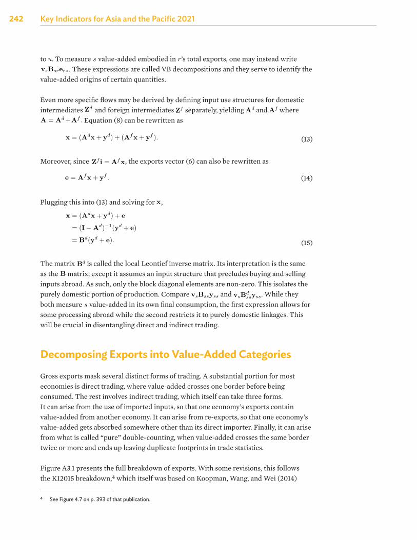
242 Key Indicators for Asia and the Pacific 2021
to
where ⊗ denote a Kronecker product. Written out,
E ≡
0 zC1,J1 + zC1,J2 zC1,U1 + zC1,U2
0 zC2,J1 + zC2,J2 zC2,U1 + zC2,U2
zJ1,C1 + zJ1,C2 0 zJ1,U1 + zJ1,U2
zJ2,C1 + zJ2,C2 0 zJ2,U1 + zJ2,U2
zU1,C1 + zU1,C2 zU1,J1 + zU1,J2 0zU2,C1 + zU2,C2 zU2,J1 + zU2,J2 0
+
0 yC1,J yC1,U
0 yC2,J yC2,U
yJ1,C 0 yJ1,U
yJ2,C 0 yJ2,U
yU1,C yU1,J 0yU2,C yU2,J 0
=
0 eC1,J eC1,U
0 eC2,J eC2,U
eJ1,C 0 eJ1,U
eJ2,C 0 eJ2,U
eU1,C eU1,J 0eU2,C eU2,J 0
=
0 eCJ eCU
eJC 0 eJU
eUC eUJ 0
The technical coefficient a(s,j),(r,i) is the share of inputs from (s, j) in the output of (r, i): a(s,j),(r,i) ≡z(s,j),(r,i)/x(r,i). Collect all these into the GN × GN matrix of technical coefficients A. This may be used torewrite (3) as
x = Ax + y. (8)
Solving for x gives
x = (I − A)−1y = By, (9)
where the GN × GN matrix B is called the global Leontief inverse matrix.
VB Decomposition
Equation (9) is central to analyzing cross-economy and cross-sectoral linkages. It is clearer to see this if (8)and (9) are rewritten to isolate a single economy s:
xs =Gr
Asrxr +Gr
ysr (10)
=Gr
Gu
Bsryru (11)
Equation (10) says that s’s output xs is used as intermediates in r’s output or sold as final goods to r (for allr = 1, ..., G). The output of each r can in turn be used as intermediates by other economies, whose outputsare then used by further economies, and so on in a potentially infinite series of production stages. Equation(11) summarizes these to identify the final landing stage of s’s output. The product Bsryru is s output thatis “completed” into a final good by r, which then sends it to u for final absorption.
In most analyses, value-added rather than output is the preferred metric. Define the vector v with (s, i)th
4
. To measure
element v(s,i) ≡ va(s,i)/x(s,i). This gives the value-added-to-output ratio for each economy–sector. It followsthat
∑(s,j) a(s,j),(r,i) + v(r,i) = 1. Premultiplying this to (11) converts everything to value-added terms:
vsxs ≡ vas = vs
G∑r
G∑u
Bsryru. (12)
Note that this ends up summing sector-level quantities into the aggregate level. To prevent this, see thesection on sector breakdowns.
This expression gives the value-added generated in economy s that is eventually consumed in economy u.It can be tweaked to measure other flows. For example, vsBsryru considers s value-added embodied infinal goods completed in r that are sold to u. To measure s value-added embodied in r’s total exports, onemay instead write vsBsrer∗. These expressions are called VB decompositions and they serve to identify thevalue-added origins of certain quantities.
Even more specific flows may be derived by defining input use structures for domestic intermediates Zd andforeign intermediates Zf separately, yielding Ad and Af where A = Ad +Af . Equation (8) can be rewrittenas
x = (Adx + yd) + (Af x + yf ). (13)
Moreover, since Zf i = Af x, the exports vector (6) can also be rewritten as
e = Af x + yf . (14)
Plugging this into (13) and solving for x,
x = (Adx + yd) + e
= (I − Ad)−1(yd + e)
= Bd(yd + e). (15)
The matrix Bd is called the local Leontief inverse matrix. Its interpretation is the same as the B matrix,except it assumes an input structure that precludes buying and selling inputs abroad. As such, only theblock diagonal elements are non-zero. This isolates the purely domestic portion of production. ComparevsBssyss and vsBd
ssyss. While they both meaure s value-added in its own final consumption, the firstexpression allows for some processing abroad while the second restricts it to purely domestic linkages. Thiswill be crucial in disentangling direct and indirect trading.
Decomposing Exports into Value-Added Categories
Gross exports mask several distinct forms of trading. A substantial portion for most economies is directtrading, where value-added crosses one border before being consumed. The rest involves indirect trading,which itself can take three forms. It can arise from the use of imported inputs, so that one economy’s exportscontain value-added from another economy. It can arise from re-exports, so that one economy’s value-addedgets absorbed somewhere other than its direct importer. Finally, it can arise from what is called “pure”
5
value-added embodied in
where ⊗ denote a Kronecker product. Written out,
E ≡
0 zC1,J1 + zC1,J2 zC1,U1 + zC1,U2
0 zC2,J1 + zC2,J2 zC2,U1 + zC2,U2
zJ1,C1 + zJ1,C2 0 zJ1,U1 + zJ1,U2
zJ2,C1 + zJ2,C2 0 zJ2,U1 + zJ2,U2
zU1,C1 + zU1,C2 zU1,J1 + zU1,J2 0zU2,C1 + zU2,C2 zU2,J1 + zU2,J2 0
+
0 yC1,J yC1,U
0 yC2,J yC2,U
yJ1,C 0 yJ1,U
yJ2,C 0 yJ2,U
yU1,C yU1,J 0yU2,C yU2,J 0
=
0 eC1,J eC1,U
0 eC2,J eC2,U
eJ1,C 0 eJ1,U
eJ2,C 0 eJ2,U
eU1,C eU1,J 0eU2,C eU2,J 0
=
0 eCJ eCU
eJC 0 eJU
eUC eUJ 0
The technical coefficient a(s,j),(r,i) is the share of inputs from (s, j) in the output of (r, i): a(s,j),(r,i) ≡z(s,j),(r,i)/x(r,i). Collect all these into the GN × GN matrix of technical coefficients A. This may be used torewrite (3) as
x = Ax + y. (8)
Solving for x gives
x = (I − A)−1y = By, (9)
where the GN × GN matrix B is called the global Leontief inverse matrix.
VB Decomposition
Equation (9) is central to analyzing cross-economy and cross-sectoral linkages. It is clearer to see this if (8)and (9) are rewritten to isolate a single economy s:
xs =Gr
Asrxr +Gr
ysr (10)
=Gr
Gu
Bsryru (11)
Equation (10) says that s’s output xs is used as intermediates in r’s output or sold as final goods to r (for allr = 1, ..., G). The output of each r can in turn be used as intermediates by other economies, whose outputsare then used by further economies, and so on in a potentially infinite series of production stages. Equation(11) summarizes these to identify the final landing stage of s’s output. The product Bsryru is s output thatis “completed” into a final good by r, which then sends it to u for final absorption.
In most analyses, value-added rather than output is the preferred metric. Define the vector v with (s, i)th
4
’s total exports, one may instead write
element v(s,i) ≡ va(s,i)/x(s,i). This gives the value-added-to-output ratio for each economy–sector. It followsthat
∑(s,j) a(s,j),(r,i) + v(r,i) = 1. Premultiplying this to (11) converts everything to value-added terms:
vsxs ≡ vas = vs
G∑r
G∑u
Bsryru. (12)
Note that this ends up summing sector-level quantities into the aggregate level. To prevent this, see thesection on sector breakdowns.
This expression gives the value-added generated in economy s that is eventually consumed in economy u.It can be tweaked to measure other flows. For example, vsBsryru considers s value-added embodied infinal goods completed in r that are sold to u. To measure s value-added embodied in r’s total exports, onemay instead write vsBsrer∗. These expressions are called VB decompositions and they serve to identify thevalue-added origins of certain quantities.
Even more specific flows may be derived by defining input use structures for domestic intermediates Zd andforeign intermediates Zf separately, yielding Ad and Af where A = Ad +Af . Equation (8) can be rewrittenas
x = (Adx + yd) + (Af x + yf ). (13)
Moreover, since Zf i = Af x, the exports vector (6) can also be rewritten as
e = Af x + yf . (14)
Plugging this into (13) and solving for x,
x = (Adx + yd) + e
= (I − Ad)−1(yd + e)
= Bd(yd + e). (15)
The matrix Bd is called the local Leontief inverse matrix. Its interpretation is the same as the B matrix,except it assumes an input structure that precludes buying and selling inputs abroad. As such, only theblock diagonal elements are non-zero. This isolates the purely domestic portion of production. ComparevsBssyss and vsBd
ssyss. While they both meaure s value-added in its own final consumption, the firstexpression allows for some processing abroad while the second restricts it to purely domestic linkages. Thiswill be crucial in disentangling direct and indirect trading.
Decomposing Exports into Value-Added Categories
Gross exports mask several distinct forms of trading. A substantial portion for most economies is directtrading, where value-added crosses one border before being consumed. The rest involves indirect trading,which itself can take three forms. It can arise from the use of imported inputs, so that one economy’s exportscontain value-added from another economy. It can arise from re-exports, so that one economy’s value-addedgets absorbed somewhere other than its direct importer. Finally, it can arise from what is called “pure”
5
. These expressions are called VB decompositions and they serve to identify the value-added origins of certain quantities.
Even more specific flows may be derived by defining input use structures for domestic intermediates
element v(s,i) ≡ va(s,i)/x(s,i). This gives the value-added-to-output ratio for each economy–sector. It followsthat
∑(s,j) a(s,j),(r,i) + v(r,i) = 1. Premultiplying this to (11) converts everything to value-added terms:
vsxs ≡ vas = vs
G∑r
G∑u
Bsryru. (12)
Note that this ends up summing sector-level quantities into the aggregate level. To prevent this, see thesection on sector breakdowns.
This expression gives the value-added generated in economy s that is eventually consumed in economy u.It can be tweaked to measure other flows. For example, vsBsryru considers s value-added embodied infinal goods completed in r that are sold to u. To measure s value-added embodied in r’s total exports, onemay instead write vsBsrer∗. These expressions are called VB decompositions and they serve to identify thevalue-added origins of certain quantities.
Even more specific flows may be derived by defining input use structures for domestic intermediates Zd andforeign intermediates Zf separately, yielding Ad and Af where A = Ad +Af . Equation (8) can be rewrittenas
x = (Adx + yd) + (Af x + yf ). (13)
Moreover, since Zf i = Af x, the exports vector (6) can also be rewritten as
e = Af x + yf . (14)
Plugging this into (13) and solving for x,
x = (Adx + yd) + e
= (I − Ad)−1(yd + e)
= Bd(yd + e). (15)
The matrix Bd is called the local Leontief inverse matrix. Its interpretation is the same as the B matrix,except it assumes an input structure that precludes buying and selling inputs abroad. As such, only theblock diagonal elements are non-zero. This isolates the purely domestic portion of production. ComparevsBssyss and vsBd
ssyss. While they both meaure s value-added in its own final consumption, the firstexpression allows for some processing abroad while the second restricts it to purely domestic linkages. Thiswill be crucial in disentangling direct and indirect trading.
Decomposing Exports into Value-Added Categories
Gross exports mask several distinct forms of trading. A substantial portion for most economies is directtrading, where value-added crosses one border before being consumed. The rest involves indirect trading,which itself can take three forms. It can arise from the use of imported inputs, so that one economy’s exportscontain value-added from another economy. It can arise from re-exports, so that one economy’s value-addedgets absorbed somewhere other than its direct importer. Finally, it can arise from what is called “pure”
5
and foreign intermediates
element v(s,i) ≡ va(s,i)/x(s,i). This gives the value-added-to-output ratio for each economy–sector. It followsthat
∑(s,j) a(s,j),(r,i) + v(r,i) = 1. Premultiplying this to (11) converts everything to value-added terms:
vsxs ≡ vas = vs
G∑r
G∑u
Bsryru. (12)
Note that this ends up summing sector-level quantities into the aggregate level. To prevent this, see thesection on sector breakdowns.
This expression gives the value-added generated in economy s that is eventually consumed in economy u.It can be tweaked to measure other flows. For example, vsBsryru considers s value-added embodied infinal goods completed in r that are sold to u. To measure s value-added embodied in r’s total exports, onemay instead write vsBsrer∗. These expressions are called VB decompositions and they serve to identify thevalue-added origins of certain quantities.
Even more specific flows may be derived by defining input use structures for domestic intermediates Zd andforeign intermediates Zf separately, yielding Ad and Af where A = Ad +Af . Equation (8) can be rewrittenas
x = (Adx + yd) + (Af x + yf ). (13)
Moreover, since Zf i = Af x, the exports vector (6) can also be rewritten as
e = Af x + yf . (14)
Plugging this into (13) and solving for x,
x = (Adx + yd) + e
= (I − Ad)−1(yd + e)
= Bd(yd + e). (15)
The matrix Bd is called the local Leontief inverse matrix. Its interpretation is the same as the B matrix,except it assumes an input structure that precludes buying and selling inputs abroad. As such, only theblock diagonal elements are non-zero. This isolates the purely domestic portion of production. ComparevsBssyss and vsBd
ssyss. While they both meaure s value-added in its own final consumption, the firstexpression allows for some processing abroad while the second restricts it to purely domestic linkages. Thiswill be crucial in disentangling direct and indirect trading.
Decomposing Exports into Value-Added Categories
Gross exports mask several distinct forms of trading. A substantial portion for most economies is directtrading, where value-added crosses one border before being consumed. The rest involves indirect trading,which itself can take three forms. It can arise from the use of imported inputs, so that one economy’s exportscontain value-added from another economy. It can arise from re-exports, so that one economy’s value-addedgets absorbed somewhere other than its direct importer. Finally, it can arise from what is called “pure”
5
separately, yielding
element v(s,i) ≡ va(s,i)/x(s,i). This gives the value-added-to-output ratio for each economy–sector. It followsthat
∑(s,j) a(s,j),(r,i) + v(r,i) = 1. Premultiplying this to (11) converts everything to value-added terms:
vsxs ≡ vas = vs
G∑r
G∑u
Bsryru. (12)
Note that this ends up summing sector-level quantities into the aggregate level. To prevent this, see thesection on sector breakdowns.
This expression gives the value-added generated in economy s that is eventually consumed in economy u.It can be tweaked to measure other flows. For example, vsBsryru considers s value-added embodied infinal goods completed in r that are sold to u. To measure s value-added embodied in r’s total exports, onemay instead write vsBsrer∗. These expressions are called VB decompositions and they serve to identify thevalue-added origins of certain quantities.
Even more specific flows may be derived by defining input use structures for domestic intermediates Zd andforeign intermediates Zf separately, yielding Ad and Af where A = Ad +Af . Equation (8) can be rewrittenas
x = (Adx + yd) + (Af x + yf ). (13)
Moreover, since Zf i = Af x, the exports vector (6) can also be rewritten as
e = Af x + yf . (14)
Plugging this into (13) and solving for x,
x = (Adx + yd) + e
= (I − Ad)−1(yd + e)
= Bd(yd + e). (15)
The matrix Bd is called the local Leontief inverse matrix. Its interpretation is the same as the B matrix,except it assumes an input structure that precludes buying and selling inputs abroad. As such, only theblock diagonal elements are non-zero. This isolates the purely domestic portion of production. ComparevsBssyss and vsBd
ssyss. While they both meaure s value-added in its own final consumption, the firstexpression allows for some processing abroad while the second restricts it to purely domestic linkages. Thiswill be crucial in disentangling direct and indirect trading.
Decomposing Exports into Value-Added Categories
Gross exports mask several distinct forms of trading. A substantial portion for most economies is directtrading, where value-added crosses one border before being consumed. The rest involves indirect trading,which itself can take three forms. It can arise from the use of imported inputs, so that one economy’s exportscontain value-added from another economy. It can arise from re-exports, so that one economy’s value-addedgets absorbed somewhere other than its direct importer. Finally, it can arise from what is called “pure”
5
and
element v(s,i) ≡ va(s,i)/x(s,i). This gives the value-added-to-output ratio for each economy–sector. It followsthat
∑(s,j) a(s,j),(r,i) + v(r,i) = 1. Premultiplying this to (11) converts everything to value-added terms:
vsxs ≡ vas = vs
G∑r
G∑u
Bsryru. (12)
Note that this ends up summing sector-level quantities into the aggregate level. To prevent this, see thesection on sector breakdowns.
This expression gives the value-added generated in economy s that is eventually consumed in economy u.It can be tweaked to measure other flows. For example, vsBsryru considers s value-added embodied infinal goods completed in r that are sold to u. To measure s value-added embodied in r’s total exports, onemay instead write vsBsrer∗. These expressions are called VB decompositions and they serve to identify thevalue-added origins of certain quantities.
Even more specific flows may be derived by defining input use structures for domestic intermediates Zd andforeign intermediates Zf separately, yielding Ad and Af where A = Ad +Af . Equation (8) can be rewrittenas
x = (Adx + yd) + (Af x + yf ). (13)
Moreover, since Zf i = Af x, the exports vector (6) can also be rewritten as
e = Af x + yf . (14)
Plugging this into (13) and solving for x,
x = (Adx + yd) + e
= (I − Ad)−1(yd + e)
= Bd(yd + e). (15)
The matrix Bd is called the local Leontief inverse matrix. Its interpretation is the same as the B matrix,except it assumes an input structure that precludes buying and selling inputs abroad. As such, only theblock diagonal elements are non-zero. This isolates the purely domestic portion of production. ComparevsBssyss and vsBd
ssyss. While they both meaure s value-added in its own final consumption, the firstexpression allows for some processing abroad while the second restricts it to purely domestic linkages. Thiswill be crucial in disentangling direct and indirect trading.
Decomposing Exports into Value-Added Categories
Gross exports mask several distinct forms of trading. A substantial portion for most economies is directtrading, where value-added crosses one border before being consumed. The rest involves indirect trading,which itself can take three forms. It can arise from the use of imported inputs, so that one economy’s exportscontain value-added from another economy. It can arise from re-exports, so that one economy’s value-addedgets absorbed somewhere other than its direct importer. Finally, it can arise from what is called “pure”
5
where
element v(s,i) ≡ va(s,i)/x(s,i). This gives the value-added-to-output ratio for each economy–sector. It followsthat
∑(s,j) a(s,j),(r,i) + v(r,i) = 1. Premultiplying this to (11) converts everything to value-added terms:
vsxs ≡ vas = vs
G∑r
G∑u
Bsryru. (12)
Note that this ends up summing sector-level quantities into the aggregate level. To prevent this, see thesection on sector breakdowns.
This expression gives the value-added generated in economy s that is eventually consumed in economy u.It can be tweaked to measure other flows. For example, vsBsryru considers s value-added embodied infinal goods completed in r that are sold to u. To measure s value-added embodied in r’s total exports, onemay instead write vsBsrer∗. These expressions are called VB decompositions and they serve to identify thevalue-added origins of certain quantities.
Even more specific flows may be derived by defining input use structures for domestic intermediates Zd andforeign intermediates Zf separately, yielding Ad and Af where A = Ad +Af . Equation (8) can be rewrittenas
x = (Adx + yd) + (Af x + yf ). (13)
Moreover, since Zf i = Af x, the exports vector (6) can also be rewritten as
e = Af x + yf . (14)
Plugging this into (13) and solving for x,
x = (Adx + yd) + e
= (I − Ad)−1(yd + e)
= Bd(yd + e). (15)
The matrix Bd is called the local Leontief inverse matrix. Its interpretation is the same as the B matrix,except it assumes an input structure that precludes buying and selling inputs abroad. As such, only theblock diagonal elements are non-zero. This isolates the purely domestic portion of production. ComparevsBssyss and vsBd
ssyss. While they both meaure s value-added in its own final consumption, the firstexpression allows for some processing abroad while the second restricts it to purely domestic linkages. Thiswill be crucial in disentangling direct and indirect trading.
Decomposing Exports into Value-Added Categories
Gross exports mask several distinct forms of trading. A substantial portion for most economies is directtrading, where value-added crosses one border before being consumed. The rest involves indirect trading,which itself can take three forms. It can arise from the use of imported inputs, so that one economy’s exportscontain value-added from another economy. It can arise from re-exports, so that one economy’s value-addedgets absorbed somewhere other than its direct importer. Finally, it can arise from what is called “pure”
5
Equation (8) can be rewritten as
element v(s,i) ≡ va(s,i)/x(s,i). This gives the value-added-to-output ratio for each economy–sector. It followsthat
∑(s,j) a(s,j),(r,i) + v(r,i) = 1. Premultiplying this to (11) converts everything to value-added terms:
vsxs ≡ vas = vs
G∑r
G∑u
Bsryru. (12)
Note that this ends up summing sector-level quantities into the aggregate level. To prevent this, see thesection on sector breakdowns.
This expression gives the value-added generated in economy s that is eventually consumed in economy u.It can be tweaked to measure other flows. For example, vsBsryru considers s value-added embodied infinal goods completed in r that are sold to u. To measure s value-added embodied in r’s total exports, onemay instead write vsBsrer∗. These expressions are called VB decompositions and they serve to identify thevalue-added origins of certain quantities.
Even more specific flows may be derived by defining input use structures for domestic intermediates Zd andforeign intermediates Zf separately, yielding Ad and Af where A = Ad +Af . Equation (8) can be rewrittenas
x = (Adx + yd) + (Af x + yf ). (13)
Moreover, since Zf i = Af x, the exports vector (6) can also be rewritten as
e = Af x + yf . (14)
Plugging this into (13) and solving for x,
x = (Adx + yd) + e
= (I − Ad)−1(yd + e)
= Bd(yd + e). (15)
The matrix Bd is called the local Leontief inverse matrix. Its interpretation is the same as the B matrix,except it assumes an input structure that precludes buying and selling inputs abroad. As such, only theblock diagonal elements are non-zero. This isolates the purely domestic portion of production. ComparevsBssyss and vsBd
ssyss. While they both meaure s value-added in its own final consumption, the firstexpression allows for some processing abroad while the second restricts it to purely domestic linkages. Thiswill be crucial in disentangling direct and indirect trading.
Decomposing Exports into Value-Added Categories
Gross exports mask several distinct forms of trading. A substantial portion for most economies is directtrading, where value-added crosses one border before being consumed. The rest involves indirect trading,which itself can take three forms. It can arise from the use of imported inputs, so that one economy’s exportscontain value-added from another economy. It can arise from re-exports, so that one economy’s value-addedgets absorbed somewhere other than its direct importer. Finally, it can arise from what is called “pure”
5
(13)
Moreover, since
element v(s,i) ≡ va(s,i)/x(s,i). This gives the value-added-to-output ratio for each economy–sector. It followsthat
∑(s,j) a(s,j),(r,i) + v(r,i) = 1. Premultiplying this to (11) converts everything to value-added terms:
vsxs ≡ vas = vs
G∑r
G∑u
Bsryru. (12)
Note that this ends up summing sector-level quantities into the aggregate level. To prevent this, see thesection on sector breakdowns.
This expression gives the value-added generated in economy s that is eventually consumed in economy u.It can be tweaked to measure other flows. For example, vsBsryru considers s value-added embodied infinal goods completed in r that are sold to u. To measure s value-added embodied in r’s total exports, onemay instead write vsBsrer∗. These expressions are called VB decompositions and they serve to identify thevalue-added origins of certain quantities.
Even more specific flows may be derived by defining input use structures for domestic intermediates Zd andforeign intermediates Zf separately, yielding Ad and Af where A = Ad +Af . Equation (8) can be rewrittenas
x = (Adx + yd) + (Af x + yf ). (13)
Moreover, since Zf i = Af x, the exports vector (6) can also be rewritten as
e = Af x + yf . (14)
Plugging this into (13) and solving for x,
x = (Adx + yd) + e
= (I − Ad)−1(yd + e)
= Bd(yd + e). (15)
The matrix Bd is called the local Leontief inverse matrix. Its interpretation is the same as the B matrix,except it assumes an input structure that precludes buying and selling inputs abroad. As such, only theblock diagonal elements are non-zero. This isolates the purely domestic portion of production. ComparevsBssyss and vsBd
ssyss. While they both meaure s value-added in its own final consumption, the firstexpression allows for some processing abroad while the second restricts it to purely domestic linkages. Thiswill be crucial in disentangling direct and indirect trading.
Decomposing Exports into Value-Added Categories
Gross exports mask several distinct forms of trading. A substantial portion for most economies is directtrading, where value-added crosses one border before being consumed. The rest involves indirect trading,which itself can take three forms. It can arise from the use of imported inputs, so that one economy’s exportscontain value-added from another economy. It can arise from re-exports, so that one economy’s value-addedgets absorbed somewhere other than its direct importer. Finally, it can arise from what is called “pure”
5
, the exports vector (6) can also be rewritten as
element v(s,i) ≡ va(s,i)/x(s,i). This gives the value-added-to-output ratio for each economy–sector. It followsthat
∑(s,j) a(s,j),(r,i) + v(r,i) = 1. Premultiplying this to (11) converts everything to value-added terms:
vsxs ≡ vas = vs
G∑r
G∑u
Bsryru. (12)
Note that this ends up summing sector-level quantities into the aggregate level. To prevent this, see thesection on sector breakdowns.
This expression gives the value-added generated in economy s that is eventually consumed in economy u.It can be tweaked to measure other flows. For example, vsBsryru considers s value-added embodied infinal goods completed in r that are sold to u. To measure s value-added embodied in r’s total exports, onemay instead write vsBsrer∗. These expressions are called VB decompositions and they serve to identify thevalue-added origins of certain quantities.
Even more specific flows may be derived by defining input use structures for domestic intermediates Zd andforeign intermediates Zf separately, yielding Ad and Af where A = Ad +Af . Equation (8) can be rewrittenas
x = (Adx + yd) + (Af x + yf ). (13)
Moreover, since Zf i = Af x, the exports vector (6) can also be rewritten as
e = Af x + yf . (14)
Plugging this into (13) and solving for x,
x = (Adx + yd) + e
= (I − Ad)−1(yd + e)
= Bd(yd + e). (15)
The matrix Bd is called the local Leontief inverse matrix. Its interpretation is the same as the B matrix,except it assumes an input structure that precludes buying and selling inputs abroad. As such, only theblock diagonal elements are non-zero. This isolates the purely domestic portion of production. ComparevsBssyss and vsBd
ssyss. While they both meaure s value-added in its own final consumption, the firstexpression allows for some processing abroad while the second restricts it to purely domestic linkages. Thiswill be crucial in disentangling direct and indirect trading.
Decomposing Exports into Value-Added Categories
Gross exports mask several distinct forms of trading. A substantial portion for most economies is directtrading, where value-added crosses one border before being consumed. The rest involves indirect trading,which itself can take three forms. It can arise from the use of imported inputs, so that one economy’s exportscontain value-added from another economy. It can arise from re-exports, so that one economy’s value-addedgets absorbed somewhere other than its direct importer. Finally, it can arise from what is called “pure”
5
(14)
Plugging this into (13) and solving for
element v(s,i) ≡ va(s,i)/x(s,i). This gives the value-added-to-output ratio for each economy–sector. It followsthat
∑(s,j) a(s,j),(r,i) + v(r,i) = 1. Premultiplying this to (11) converts everything to value-added terms:
vsxs ≡ vas = vs
G∑r
G∑u
Bsryru. (12)
Note that this ends up summing sector-level quantities into the aggregate level. To prevent this, see thesection on sector breakdowns.
This expression gives the value-added generated in economy s that is eventually consumed in economy u.It can be tweaked to measure other flows. For example, vsBsryru considers s value-added embodied infinal goods completed in r that are sold to u. To measure s value-added embodied in r’s total exports, onemay instead write vsBsrer∗. These expressions are called VB decompositions and they serve to identify thevalue-added origins of certain quantities.
Even more specific flows may be derived by defining input use structures for domestic intermediates Zd andforeign intermediates Zf separately, yielding Ad and Af where A = Ad +Af . Equation (8) can be rewrittenas
x = (Adx + yd) + (Af x + yf ). (13)
Moreover, since Zf i = Af x, the exports vector (6) can also be rewritten as
e = Af x + yf . (14)
Plugging this into (13) and solving for x,
x = (Adx + yd) + e
= (I − Ad)−1(yd + e)
= Bd(yd + e). (15)
The matrix Bd is called the local Leontief inverse matrix. Its interpretation is the same as the B matrix,except it assumes an input structure that precludes buying and selling inputs abroad. As such, only theblock diagonal elements are non-zero. This isolates the purely domestic portion of production. ComparevsBssyss and vsBd
ssyss. While they both meaure s value-added in its own final consumption, the firstexpression allows for some processing abroad while the second restricts it to purely domestic linkages. Thiswill be crucial in disentangling direct and indirect trading.
Decomposing Exports into Value-Added Categories
Gross exports mask several distinct forms of trading. A substantial portion for most economies is directtrading, where value-added crosses one border before being consumed. The rest involves indirect trading,which itself can take three forms. It can arise from the use of imported inputs, so that one economy’s exportscontain value-added from another economy. It can arise from re-exports, so that one economy’s value-addedgets absorbed somewhere other than its direct importer. Finally, it can arise from what is called “pure”
5
,
element v(s,i) ≡ va(s,i)/x(s,i). This gives the value-added-to-output ratio for each economy–sector. It followsthat
∑(s,j) a(s,j),(r,i) + v(r,i) = 1. Premultiplying this to (11) converts everything to value-added terms:
vsxs ≡ vas = vs
G∑r
G∑u
Bsryru. (12)
Note that this ends up summing sector-level quantities into the aggregate level. To prevent this, see thesection on sector breakdowns.
This expression gives the value-added generated in economy s that is eventually consumed in economy u.It can be tweaked to measure other flows. For example, vsBsryru considers s value-added embodied infinal goods completed in r that are sold to u. To measure s value-added embodied in r’s total exports, onemay instead write vsBsrer∗. These expressions are called VB decompositions and they serve to identify thevalue-added origins of certain quantities.
Even more specific flows may be derived by defining input use structures for domestic intermediates Zd andforeign intermediates Zf separately, yielding Ad and Af where A = Ad +Af . Equation (8) can be rewrittenas
x = (Adx + yd) + (Af x + yf ). (13)
Moreover, since Zf i = Af x, the exports vector (6) can also be rewritten as
e = Af x + yf . (14)
Plugging this into (13) and solving for x,
x = (Adx + yd) + e
= (I − Ad)−1(yd + e)
= Bd(yd + e). (15)
The matrix Bd is called the local Leontief inverse matrix. Its interpretation is the same as the B matrix,except it assumes an input structure that precludes buying and selling inputs abroad. As such, only theblock diagonal elements are non-zero. This isolates the purely domestic portion of production. ComparevsBssyss and vsBd
ssyss. While they both meaure s value-added in its own final consumption, the firstexpression allows for some processing abroad while the second restricts it to purely domestic linkages. Thiswill be crucial in disentangling direct and indirect trading.
Decomposing Exports into Value-Added Categories
Gross exports mask several distinct forms of trading. A substantial portion for most economies is directtrading, where value-added crosses one border before being consumed. The rest involves indirect trading,which itself can take three forms. It can arise from the use of imported inputs, so that one economy’s exportscontain value-added from another economy. It can arise from re-exports, so that one economy’s value-addedgets absorbed somewhere other than its direct importer. Finally, it can arise from what is called “pure”
5
(15)
The matrix
element v(s,i) ≡ va(s,i)/x(s,i). This gives the value-added-to-output ratio for each economy–sector. It followsthat
∑(s,j) a(s,j),(r,i) + v(r,i) = 1. Premultiplying this to (11) converts everything to value-added terms:
vsxs ≡ vas = vs
G∑r
G∑u
Bsryru. (12)
Note that this ends up summing sector-level quantities into the aggregate level. To prevent this, see thesection on sector breakdowns.
This expression gives the value-added generated in economy s that is eventually consumed in economy u.It can be tweaked to measure other flows. For example, vsBsryru considers s value-added embodied infinal goods completed in r that are sold to u. To measure s value-added embodied in r’s total exports, onemay instead write vsBsrer∗. These expressions are called VB decompositions and they serve to identify thevalue-added origins of certain quantities.
Even more specific flows may be derived by defining input use structures for domestic intermediates Zd andforeign intermediates Zf separately, yielding Ad and Af where A = Ad +Af . Equation (8) can be rewrittenas
x = (Adx + yd) + (Af x + yf ). (13)
Moreover, since Zf i = Af x, the exports vector (6) can also be rewritten as
e = Af x + yf . (14)
Plugging this into (13) and solving for x,
x = (Adx + yd) + e
= (I − Ad)−1(yd + e)
= Bd(yd + e). (15)
The matrix Bd is called the local Leontief inverse matrix. Its interpretation is the same as the B matrix,except it assumes an input structure that precludes buying and selling inputs abroad. As such, only theblock diagonal elements are non-zero. This isolates the purely domestic portion of production. ComparevsBssyss and vsBd
ssyss. While they both meaure s value-added in its own final consumption, the firstexpression allows for some processing abroad while the second restricts it to purely domestic linkages. Thiswill be crucial in disentangling direct and indirect trading.
Decomposing Exports into Value-Added Categories
Gross exports mask several distinct forms of trading. A substantial portion for most economies is directtrading, where value-added crosses one border before being consumed. The rest involves indirect trading,which itself can take three forms. It can arise from the use of imported inputs, so that one economy’s exportscontain value-added from another economy. It can arise from re-exports, so that one economy’s value-addedgets absorbed somewhere other than its direct importer. Finally, it can arise from what is called “pure”
5
is called the local Leontief inverse matrix. Its interpretation is the same as the
element v(s,i) ≡ va(s,i)/x(s,i). This gives the value-added-to-output ratio for each economy–sector. It followsthat
∑(s,j) a(s,j),(r,i) + v(r,i) = 1. Premultiplying this to (11) converts everything to value-added terms:
vsxs ≡ vas = vs
G∑r
G∑u
Bsryru. (12)
Note that this ends up summing sector-level quantities into the aggregate level. To prevent this, see thesection on sector breakdowns.
This expression gives the value-added generated in economy s that is eventually consumed in economy u.It can be tweaked to measure other flows. For example, vsBsryru considers s value-added embodied infinal goods completed in r that are sold to u. To measure s value-added embodied in r’s total exports, onemay instead write vsBsrer∗. These expressions are called VB decompositions and they serve to identify thevalue-added origins of certain quantities.
Even more specific flows may be derived by defining input use structures for domestic intermediates Zd andforeign intermediates Zf separately, yielding Ad and Af where A = Ad +Af . Equation (8) can be rewrittenas
x = (Adx + yd) + (Af x + yf ). (13)
Moreover, since Zf i = Af x, the exports vector (6) can also be rewritten as
e = Af x + yf . (14)
Plugging this into (13) and solving for x,
x = (Adx + yd) + e
= (I − Ad)−1(yd + e)
= Bd(yd + e). (15)
The matrix Bd is called the local Leontief inverse matrix. Its interpretation is the same as the B matrix,except it assumes an input structure that precludes buying and selling inputs abroad. As such, only theblock diagonal elements are non-zero. This isolates the purely domestic portion of production. ComparevsBssyss and vsBd
ssyss. While they both meaure s value-added in its own final consumption, the firstexpression allows for some processing abroad while the second restricts it to purely domestic linkages. Thiswill be crucial in disentangling direct and indirect trading.
Decomposing Exports into Value-Added Categories
Gross exports mask several distinct forms of trading. A substantial portion for most economies is directtrading, where value-added crosses one border before being consumed. The rest involves indirect trading,which itself can take three forms. It can arise from the use of imported inputs, so that one economy’s exportscontain value-added from another economy. It can arise from re-exports, so that one economy’s value-addedgets absorbed somewhere other than its direct importer. Finally, it can arise from what is called “pure”
5
matrix, except it assumes an input structure that precludes buying and selling inputs abroad. As such, only the block diagonal elements are non-zero. This isolates the purely domestic portion of production. Compare
element v(s,i) ≡ va(s,i)/x(s,i). This gives the value-added-to-output ratio for each economy–sector. It followsthat
∑(s,j) a(s,j),(r,i) + v(r,i) = 1. Premultiplying this to (11) converts everything to value-added terms:
vsxs ≡ vas = vs
G∑r
G∑u
Bsryru. (12)
Note that this ends up summing sector-level quantities into the aggregate level. To prevent this, see thesection on sector breakdowns.
This expression gives the value-added generated in economy s that is eventually consumed in economy u.It can be tweaked to measure other flows. For example, vsBsryru considers s value-added embodied infinal goods completed in r that are sold to u. To measure s value-added embodied in r’s total exports, onemay instead write vsBsrer∗. These expressions are called VB decompositions and they serve to identify thevalue-added origins of certain quantities.
Even more specific flows may be derived by defining input use structures for domestic intermediates Zd andforeign intermediates Zf separately, yielding Ad and Af where A = Ad +Af . Equation (8) can be rewrittenas
x = (Adx + yd) + (Af x + yf ). (13)
Moreover, since Zf i = Af x, the exports vector (6) can also be rewritten as
e = Af x + yf . (14)
Plugging this into (13) and solving for x,
x = (Adx + yd) + e
= (I − Ad)−1(yd + e)
= Bd(yd + e). (15)
The matrix Bd is called the local Leontief inverse matrix. Its interpretation is the same as the B matrix,except it assumes an input structure that precludes buying and selling inputs abroad. As such, only theblock diagonal elements are non-zero. This isolates the purely domestic portion of production. ComparevsBssyss and vsBd
ssyss. While they both meaure s value-added in its own final consumption, the firstexpression allows for some processing abroad while the second restricts it to purely domestic linkages. Thiswill be crucial in disentangling direct and indirect trading.
Decomposing Exports into Value-Added Categories
Gross exports mask several distinct forms of trading. A substantial portion for most economies is directtrading, where value-added crosses one border before being consumed. The rest involves indirect trading,which itself can take three forms. It can arise from the use of imported inputs, so that one economy’s exportscontain value-added from another economy. It can arise from re-exports, so that one economy’s value-addedgets absorbed somewhere other than its direct importer. Finally, it can arise from what is called “pure”
5
and
element v(s,i) ≡ va(s,i)/x(s,i). This gives the value-added-to-output ratio for each economy–sector. It followsthat
∑(s,j) a(s,j),(r,i) + v(r,i) = 1. Premultiplying this to (11) converts everything to value-added terms:
vsxs ≡ vas = vs
G∑r
G∑u
Bsryru. (12)
Note that this ends up summing sector-level quantities into the aggregate level. To prevent this, see thesection on sector breakdowns.
This expression gives the value-added generated in economy s that is eventually consumed in economy u.It can be tweaked to measure other flows. For example, vsBsryru considers s value-added embodied infinal goods completed in r that are sold to u. To measure s value-added embodied in r’s total exports, onemay instead write vsBsrer∗. These expressions are called VB decompositions and they serve to identify thevalue-added origins of certain quantities.
Even more specific flows may be derived by defining input use structures for domestic intermediates Zd andforeign intermediates Zf separately, yielding Ad and Af where A = Ad +Af . Equation (8) can be rewrittenas
x = (Adx + yd) + (Af x + yf ). (13)
Moreover, since Zf i = Af x, the exports vector (6) can also be rewritten as
e = Af x + yf . (14)
Plugging this into (13) and solving for x,
x = (Adx + yd) + e
= (I − Ad)−1(yd + e)
= Bd(yd + e). (15)
The matrix Bd is called the local Leontief inverse matrix. Its interpretation is the same as the B matrix,except it assumes an input structure that precludes buying and selling inputs abroad. As such, only theblock diagonal elements are non-zero. This isolates the purely domestic portion of production. ComparevsBssyss and vsBd
ssyss. While they both meaure s value-added in its own final consumption, the firstexpression allows for some processing abroad while the second restricts it to purely domestic linkages. Thiswill be crucial in disentangling direct and indirect trading.
Decomposing Exports into Value-Added Categories
Gross exports mask several distinct forms of trading. A substantial portion for most economies is directtrading, where value-added crosses one border before being consumed. The rest involves indirect trading,which itself can take three forms. It can arise from the use of imported inputs, so that one economy’s exportscontain value-added from another economy. It can arise from re-exports, so that one economy’s value-addedgets absorbed somewhere other than its direct importer. Finally, it can arise from what is called “pure”
5
. While they both measure
element v(s,i) ≡ va(s,i)/x(s,i). This gives the value-added-to-output ratio for each economy–sector. It followsthat
∑(s,j) a(s,j),(r,i) + v(r,i) = 1. Premultiplying this to (11) converts everything to value-added terms:
vsxs ≡ vas = vs
G∑r
G∑u
Bsryru. (12)
Note that this ends up summing sector-level quantities into the aggregate level. To prevent this, see thesection on sector breakdowns.
This expression gives the value-added generated in economy s that is eventually consumed in economy u.It can be tweaked to measure other flows. For example, vsBsryru considers s value-added embodied infinal goods completed in r that are sold to u. To measure s value-added embodied in r’s total exports, onemay instead write vsBsrer∗. These expressions are called VB decompositions and they serve to identify thevalue-added origins of certain quantities.
Even more specific flows may be derived by defining input use structures for domestic intermediates Zd andforeign intermediates Zf separately, yielding Ad and Af where A = Ad +Af . Equation (8) can be rewrittenas
x = (Adx + yd) + (Af x + yf ). (13)
Moreover, since Zf i = Af x, the exports vector (6) can also be rewritten as
e = Af x + yf . (14)
Plugging this into (13) and solving for x,
x = (Adx + yd) + e
= (I − Ad)−1(yd + e)
= Bd(yd + e). (15)
The matrix Bd is called the local Leontief inverse matrix. Its interpretation is the same as the B matrix,except it assumes an input structure that precludes buying and selling inputs abroad. As such, only theblock diagonal elements are non-zero. This isolates the purely domestic portion of production. ComparevsBssyss and vsBd
ssyss. While they both meaure s value-added in its own final consumption, the firstexpression allows for some processing abroad while the second restricts it to purely domestic linkages. Thiswill be crucial in disentangling direct and indirect trading.
Decomposing Exports into Value-Added Categories
Gross exports mask several distinct forms of trading. A substantial portion for most economies is directtrading, where value-added crosses one border before being consumed. The rest involves indirect trading,which itself can take three forms. It can arise from the use of imported inputs, so that one economy’s exportscontain value-added from another economy. It can arise from re-exports, so that one economy’s value-addedgets absorbed somewhere other than its direct importer. Finally, it can arise from what is called “pure”
5
value-added in its own final consumption, the first expression allows for some processing abroad while the second restricts it to purely domestic linkages. This will be crucial in disentangling direct and indirect trading.
Decomposing Exports into Value-Added Categories
Gross exports mask several distinct forms of trading. A substantial portion for most economies is direct trading, where value-added crosses one border before being consumed. The rest involves indirect trading, which itself can take three forms. It can arise from the use of imported inputs, so that one economy’s exports contain value-added from another economy. It can arise from re-exports, so that one economy’s value-added gets absorbed somewhere other than its direct importer. Finally, it can arise from what is called “pure” double-counting, when value-added crosses the same border twice or more and ends up leaving duplicate footprints in trade statistics.
Figure A3.1 presents the full breakdown of exports. With some revisions, this follows the KI2015 breakdown,4 which itself was based on Koopman, Wang, and Wei (2014)
4 See Figure 4.7 on p. 393 of that publication.
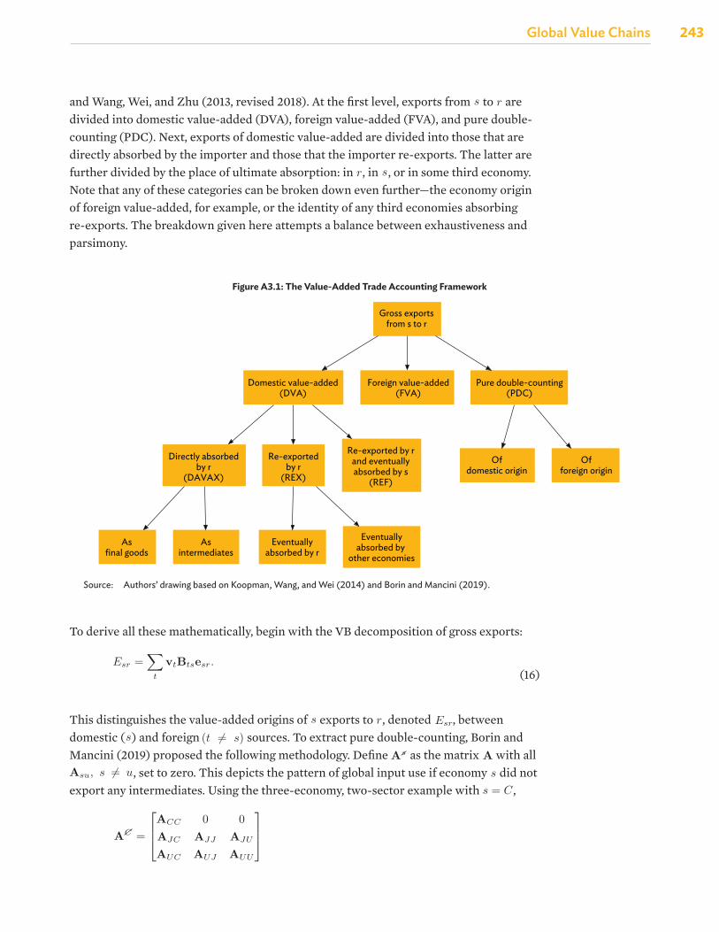
Global Value Chains
243Global Value Chains
and Wang, Wei, and Zhu (2013, revised 2018). At the first level, exports from
element v(s,i) ≡ va(s,i)/x(s,i). This gives the value-added-to-output ratio for each economy–sector. It followsthat
∑(s,j) a(s,j),(r,i) + v(r,i) = 1. Premultiplying this to (11) converts everything to value-added terms:
vsxs ≡ vas = vs
G∑r
G∑u
Bsryru. (12)
Note that this ends up summing sector-level quantities into the aggregate level. To prevent this, see thesection on sector breakdowns.
This expression gives the value-added generated in economy s that is eventually consumed in economy u.It can be tweaked to measure other flows. For example, vsBsryru considers s value-added embodied infinal goods completed in r that are sold to u. To measure s value-added embodied in r’s total exports, onemay instead write vsBsrer∗. These expressions are called VB decompositions and they serve to identify thevalue-added origins of certain quantities.
Even more specific flows may be derived by defining input use structures for domestic intermediates Zd andforeign intermediates Zf separately, yielding Ad and Af where A = Ad +Af . Equation (8) can be rewrittenas
x = (Adx + yd) + (Af x + yf ). (13)
Moreover, since Zf i = Af x, the exports vector (6) can also be rewritten as
e = Af x + yf . (14)
Plugging this into (13) and solving for x,
x = (Adx + yd) + e
= (I − Ad)−1(yd + e)
= Bd(yd + e). (15)
The matrix Bd is called the local Leontief inverse matrix. Its interpretation is the same as the B matrix,except it assumes an input structure that precludes buying and selling inputs abroad. As such, only theblock diagonal elements are non-zero. This isolates the purely domestic portion of production. ComparevsBssyss and vsBd
ssyss. While they both meaure s value-added in its own final consumption, the firstexpression allows for some processing abroad while the second restricts it to purely domestic linkages. Thiswill be crucial in disentangling direct and indirect trading.
Decomposing Exports into Value-Added Categories
Gross exports mask several distinct forms of trading. A substantial portion for most economies is directtrading, where value-added crosses one border before being consumed. The rest involves indirect trading,which itself can take three forms. It can arise from the use of imported inputs, so that one economy’s exportscontain value-added from another economy. It can arise from re-exports, so that one economy’s value-addedgets absorbed somewhere other than its direct importer. Finally, it can arise from what is called “pure”
5
to
where ⊗ denote a Kronecker product. Written out,
E ≡
0 zC1,J1 + zC1,J2 zC1,U1 + zC1,U2
0 zC2,J1 + zC2,J2 zC2,U1 + zC2,U2
zJ1,C1 + zJ1,C2 0 zJ1,U1 + zJ1,U2
zJ2,C1 + zJ2,C2 0 zJ2,U1 + zJ2,U2
zU1,C1 + zU1,C2 zU1,J1 + zU1,J2 0zU2,C1 + zU2,C2 zU2,J1 + zU2,J2 0
+
0 yC1,J yC1,U
0 yC2,J yC2,U
yJ1,C 0 yJ1,U
yJ2,C 0 yJ2,U
yU1,C yU1,J 0yU2,C yU2,J 0
=
0 eC1,J eC1,U
0 eC2,J eC2,U
eJ1,C 0 eJ1,U
eJ2,C 0 eJ2,U
eU1,C eU1,J 0eU2,C eU2,J 0
=
0 eCJ eCU
eJC 0 eJU
eUC eUJ 0
The technical coefficient a(s,j),(r,i) is the share of inputs from (s, j) in the output of (r, i): a(s,j),(r,i) ≡z(s,j),(r,i)/x(r,i). Collect all these into the GN × GN matrix of technical coefficients A. This may be used torewrite (3) as
x = Ax + y. (8)
Solving for x gives
x = (I − A)−1y = By, (9)
where the GN × GN matrix B is called the global Leontief inverse matrix.
VB Decomposition
Equation (9) is central to analyzing cross-economy and cross-sectoral linkages. It is clearer to see this if (8)and (9) are rewritten to isolate a single economy s:
xs =Gr
Asrxr +Gr
ysr (10)
=Gr
Gu
Bsryru (11)
Equation (10) says that s’s output xs is used as intermediates in r’s output or sold as final goods to r (for allr = 1, ..., G). The output of each r can in turn be used as intermediates by other economies, whose outputsare then used by further economies, and so on in a potentially infinite series of production stages. Equation(11) summarizes these to identify the final landing stage of s’s output. The product Bsryru is s output thatis “completed” into a final good by r, which then sends it to u for final absorption.
In most analyses, value-added rather than output is the preferred metric. Define the vector v with (s, i)th
4
are divided into domestic value-added (DVA), foreign value-added (FVA), and pure double-counting (PDC). Next, exports of domestic value-added are divided into those that are directly absorbed by the importer and those that the importer re-exports. The latter are further divided by the place of ultimate absorption: in
where ⊗ denote a Kronecker product. Written out,
E ≡
0 zC1,J1 + zC1,J2 zC1,U1 + zC1,U2
0 zC2,J1 + zC2,J2 zC2,U1 + zC2,U2
zJ1,C1 + zJ1,C2 0 zJ1,U1 + zJ1,U2
zJ2,C1 + zJ2,C2 0 zJ2,U1 + zJ2,U2
zU1,C1 + zU1,C2 zU1,J1 + zU1,J2 0zU2,C1 + zU2,C2 zU2,J1 + zU2,J2 0
+
0 yC1,J yC1,U
0 yC2,J yC2,U
yJ1,C 0 yJ1,U
yJ2,C 0 yJ2,U
yU1,C yU1,J 0yU2,C yU2,J 0
=
0 eC1,J eC1,U
0 eC2,J eC2,U
eJ1,C 0 eJ1,U
eJ2,C 0 eJ2,U
eU1,C eU1,J 0eU2,C eU2,J 0
=
0 eCJ eCU
eJC 0 eJU
eUC eUJ 0
The technical coefficient a(s,j),(r,i) is the share of inputs from (s, j) in the output of (r, i): a(s,j),(r,i) ≡z(s,j),(r,i)/x(r,i). Collect all these into the GN × GN matrix of technical coefficients A. This may be used torewrite (3) as
x = Ax + y. (8)
Solving for x gives
x = (I − A)−1y = By, (9)
where the GN × GN matrix B is called the global Leontief inverse matrix.
VB Decomposition
Equation (9) is central to analyzing cross-economy and cross-sectoral linkages. It is clearer to see this if (8)and (9) are rewritten to isolate a single economy s:
xs =Gr
Asrxr +Gr
ysr (10)
=Gr
Gu
Bsryru (11)
Equation (10) says that s’s output xs is used as intermediates in r’s output or sold as final goods to r (for allr = 1, ..., G). The output of each r can in turn be used as intermediates by other economies, whose outputsare then used by further economies, and so on in a potentially infinite series of production stages. Equation(11) summarizes these to identify the final landing stage of s’s output. The product Bsryru is s output thatis “completed” into a final good by r, which then sends it to u for final absorption.
In most analyses, value-added rather than output is the preferred metric. Define the vector v with (s, i)th
4
, in
element v(s,i) ≡ va(s,i)/x(s,i). This gives the value-added-to-output ratio for each economy–sector. It followsthat
∑(s,j) a(s,j),(r,i) + v(r,i) = 1. Premultiplying this to (11) converts everything to value-added terms:
vsxs ≡ vas = vs
G∑r
G∑u
Bsryru. (12)
Note that this ends up summing sector-level quantities into the aggregate level. To prevent this, see thesection on sector breakdowns.
This expression gives the value-added generated in economy s that is eventually consumed in economy u.It can be tweaked to measure other flows. For example, vsBsryru considers s value-added embodied infinal goods completed in r that are sold to u. To measure s value-added embodied in r’s total exports, onemay instead write vsBsrer∗. These expressions are called VB decompositions and they serve to identify thevalue-added origins of certain quantities.
Even more specific flows may be derived by defining input use structures for domestic intermediates Zd andforeign intermediates Zf separately, yielding Ad and Af where A = Ad +Af . Equation (8) can be rewrittenas
x = (Adx + yd) + (Af x + yf ). (13)
Moreover, since Zf i = Af x, the exports vector (6) can also be rewritten as
e = Af x + yf . (14)
Plugging this into (13) and solving for x,
x = (Adx + yd) + e
= (I − Ad)−1(yd + e)
= Bd(yd + e). (15)
The matrix Bd is called the local Leontief inverse matrix. Its interpretation is the same as the B matrix,except it assumes an input structure that precludes buying and selling inputs abroad. As such, only theblock diagonal elements are non-zero. This isolates the purely domestic portion of production. ComparevsBssyss and vsBd
ssyss. While they both meaure s value-added in its own final consumption, the firstexpression allows for some processing abroad while the second restricts it to purely domestic linkages. Thiswill be crucial in disentangling direct and indirect trading.
Decomposing Exports into Value-Added Categories
Gross exports mask several distinct forms of trading. A substantial portion for most economies is directtrading, where value-added crosses one border before being consumed. The rest involves indirect trading,which itself can take three forms. It can arise from the use of imported inputs, so that one economy’s exportscontain value-added from another economy. It can arise from re-exports, so that one economy’s value-addedgets absorbed somewhere other than its direct importer. Finally, it can arise from what is called “pure”
5
, or in some third economy. Note that any of these categories can be broken down even further—the economy origin of foreign value-added, for example, or the identity of any third economies absorbing re-exports. The breakdown given here attempts a balance between exhaustiveness and parsimony.
Figure A3.1: The Value-Added Trade Accounting Framework
Gross exportsfrom s to r
Domestic value-added(DVA)
Directly absorbedby r
(DAVAX)
Asfinal goods
Asintermediates
Eventuallyabsorbed by r
Eventuallyabsorbed by
other economies
Re-exportedby r
(REX)
Ofdomestic origin
Offoreign origin
Re-exported by rand eventuallyabsorbed by s
(REF)
Foreign value-added(FVA)
Pure double-counting(PDC)
Source: Authors’ drawing based on Koopman, Wang, and Wei (2014) and Borin and Mancini (2019).
To derive all these mathematically, begin with the VB decomposition of gross exports:
double-counting, when value-added crosses the same border twice or more and ends up leaving duplicatefootprints in trade statistics.
Figure A3.1.1 presents the full breakdown of exports. With some revisions, this follows the KI2015breakdown3, which itself was based on Koopman, Wang, and Wei (2014) and Wang, Wei, and Zhu (2013,revised 2018). At the first level, exports from s to r are divided into domestic value-added (DVA), foreignvalue-added (FVA), and pure double-counting (PDC). Next, exports of domestic value-added are dividedinto those that are directly absorbed by the importer and those that the importer re-exports. The latter arefurther divided by the place of ultimate absorption: in r, in s, or in some third economy. Note that any ofthese categories can be broken down even further—the economy origin of foreign value-added, for example,or the identity of any third economies absorbing re-exports. The breakdown given here attempts a balancebetween exhaustiveness and parsimony.
Figure A3.1.1: The Value-Added Trade Accounting Framework
Gross exports
from s to r
Domestic value-added
(DVA)
Foreign value-added
(FVA)
Pure double-counting
(PDC)
Directly absorbed
by r
(DAVAX)
Re-exported
by r
(REX)
Re-exported by r
and eventually
absorbed by s
(REF)
As
final goods
As
intermediates
Of
domestic origin
Of
foreign origin
Eventually
absorbed by r
Eventually
absorbed by
other economies
Source: Authors’ drawing based on Koopman, Wang, and Wei (2014) and Borin and Mancini (2019).
To derive all these mathematically, begin with the VB decomposition of gross exports:
Esr =∑
t
vtBtsesr. (16)
This distinguishes the value-added origins of s exports to r, denoted Esr, between domestic (s) and foreign(t = s) sources. To extract pure double-counting, Borin and Mancini (2019) proposed the followingmethodology. Define As as the matrix A with all Asu, s = u, set to zero. This depicts the patternof global input use if economy s did not export any intermediates. Using the three-economy, two-sector
3See Figure 4.7 on p. 393 of that publication.
6
(16)
This distinguishes the value-added origins of
element v(s,i) ≡ va(s,i)/x(s,i). This gives the value-added-to-output ratio for each economy–sector. It followsthat
∑(s,j) a(s,j),(r,i) + v(r,i) = 1. Premultiplying this to (11) converts everything to value-added terms:
vsxs ≡ vas = vs
G∑r
G∑u
Bsryru. (12)
Note that this ends up summing sector-level quantities into the aggregate level. To prevent this, see thesection on sector breakdowns.
This expression gives the value-added generated in economy s that is eventually consumed in economy u.It can be tweaked to measure other flows. For example, vsBsryru considers s value-added embodied infinal goods completed in r that are sold to u. To measure s value-added embodied in r’s total exports, onemay instead write vsBsrer∗. These expressions are called VB decompositions and they serve to identify thevalue-added origins of certain quantities.
Even more specific flows may be derived by defining input use structures for domestic intermediates Zd andforeign intermediates Zf separately, yielding Ad and Af where A = Ad +Af . Equation (8) can be rewrittenas
x = (Adx + yd) + (Af x + yf ). (13)
Moreover, since Zf i = Af x, the exports vector (6) can also be rewritten as
e = Af x + yf . (14)
Plugging this into (13) and solving for x,
x = (Adx + yd) + e
= (I − Ad)−1(yd + e)
= Bd(yd + e). (15)
The matrix Bd is called the local Leontief inverse matrix. Its interpretation is the same as the B matrix,except it assumes an input structure that precludes buying and selling inputs abroad. As such, only theblock diagonal elements are non-zero. This isolates the purely domestic portion of production. ComparevsBssyss and vsBd
ssyss. While they both meaure s value-added in its own final consumption, the firstexpression allows for some processing abroad while the second restricts it to purely domestic linkages. Thiswill be crucial in disentangling direct and indirect trading.
Decomposing Exports into Value-Added Categories
Gross exports mask several distinct forms of trading. A substantial portion for most economies is directtrading, where value-added crosses one border before being consumed. The rest involves indirect trading,which itself can take three forms. It can arise from the use of imported inputs, so that one economy’s exportscontain value-added from another economy. It can arise from re-exports, so that one economy’s value-addedgets absorbed somewhere other than its direct importer. Finally, it can arise from what is called “pure”
5
exports to
where ⊗ denote a Kronecker product. Written out,
E ≡
0 zC1,J1 + zC1,J2 zC1,U1 + zC1,U2
0 zC2,J1 + zC2,J2 zC2,U1 + zC2,U2
zJ1,C1 + zJ1,C2 0 zJ1,U1 + zJ1,U2
zJ2,C1 + zJ2,C2 0 zJ2,U1 + zJ2,U2
zU1,C1 + zU1,C2 zU1,J1 + zU1,J2 0zU2,C1 + zU2,C2 zU2,J1 + zU2,J2 0
+
0 yC1,J yC1,U
0 yC2,J yC2,U
yJ1,C 0 yJ1,U
yJ2,C 0 yJ2,U
yU1,C yU1,J 0yU2,C yU2,J 0
=
0 eC1,J eC1,U
0 eC2,J eC2,U
eJ1,C 0 eJ1,U
eJ2,C 0 eJ2,U
eU1,C eU1,J 0eU2,C eU2,J 0
=
0 eCJ eCU
eJC 0 eJU
eUC eUJ 0
The technical coefficient a(s,j),(r,i) is the share of inputs from (s, j) in the output of (r, i): a(s,j),(r,i) ≡z(s,j),(r,i)/x(r,i). Collect all these into the GN × GN matrix of technical coefficients A. This may be used torewrite (3) as
x = Ax + y. (8)
Solving for x gives
x = (I − A)−1y = By, (9)
where the GN × GN matrix B is called the global Leontief inverse matrix.
VB Decomposition
Equation (9) is central to analyzing cross-economy and cross-sectoral linkages. It is clearer to see this if (8)and (9) are rewritten to isolate a single economy s:
xs =Gr
Asrxr +Gr
ysr (10)
=Gr
Gu
Bsryru (11)
Equation (10) says that s’s output xs is used as intermediates in r’s output or sold as final goods to r (for allr = 1, ..., G). The output of each r can in turn be used as intermediates by other economies, whose outputsare then used by further economies, and so on in a potentially infinite series of production stages. Equation(11) summarizes these to identify the final landing stage of s’s output. The product Bsryru is s output thatis “completed” into a final good by r, which then sends it to u for final absorption.
In most analyses, value-added rather than output is the preferred metric. Define the vector v with (s, i)th
4
, denoted
double-counting, when value-added crosses the same border twice or more and ends up leaving duplicatefootprints in trade statistics.
Figure A3.1.1 presents the full breakdown of exports. With some revisions, this follows the KI2015breakdown3, which itself was based on Koopman, Wang, and Wei (2014) and Wang, Wei, and Zhu (2013,revised 2018). At the first level, exports from s to r are divided into domestic value-added (DVA), foreignvalue-added (FVA), and pure double-counting (PDC). Next, exports of domestic value-added are dividedinto those that are directly absorbed by the importer and those that the importer re-exports. The latter arefurther divided by the place of ultimate absorption: in r, in s, or in some third economy. Note that any ofthese categories can be broken down even further—the economy origin of foreign value-added, for example,or the identity of any third economies absorbing re-exports. The breakdown given here attempts a balancebetween exhaustiveness and parsimony.
Figure A3.1.1: The Value-Added Trade Accounting Framework
Gross exports
from s to r
Domestic value-added
(DVA)
Foreign value-added
(FVA)
Pure double-counting
(PDC)
Directly absorbed
by r
(DAVAX)
Re-exported
by r
(REX)
Re-exported by r
and eventually
absorbed by s
(REF)
As
final goods
As
intermediates
Of
domestic origin
Of
foreign origin
Eventually
absorbed by r
Eventually
absorbed by
other economies
Source: Authors’ drawing based on Koopman, Wang, and Wei (2014) and Borin and Mancini (2019).
To derive all these mathematically, begin with the VB decomposition of gross exports:
Esr =∑
t
vtBtsesr. (16)
This distinguishes the value-added origins of s exports to r, denoted Esr, between domestic (s) and foreign(t = s) sources. To extract pure double-counting, Borin and Mancini (2019) proposed the followingmethodology. Define As as the matrix A with all Asu, s = u, set to zero. This depicts the patternof global input use if economy s did not export any intermediates. Using the three-economy, two-sector
3See Figure 4.7 on p. 393 of that publication.
6
, between domestic (
element v(s,i) ≡ va(s,i)/x(s,i). This gives the value-added-to-output ratio for each economy–sector. It followsthat
∑(s,j) a(s,j),(r,i) + v(r,i) = 1. Premultiplying this to (11) converts everything to value-added terms:
vsxs ≡ vas = vs
G∑r
G∑u
Bsryru. (12)
Note that this ends up summing sector-level quantities into the aggregate level. To prevent this, see thesection on sector breakdowns.
This expression gives the value-added generated in economy s that is eventually consumed in economy u.It can be tweaked to measure other flows. For example, vsBsryru considers s value-added embodied infinal goods completed in r that are sold to u. To measure s value-added embodied in r’s total exports, onemay instead write vsBsrer∗. These expressions are called VB decompositions and they serve to identify thevalue-added origins of certain quantities.
Even more specific flows may be derived by defining input use structures for domestic intermediates Zd andforeign intermediates Zf separately, yielding Ad and Af where A = Ad +Af . Equation (8) can be rewrittenas
x = (Adx + yd) + (Af x + yf ). (13)
Moreover, since Zf i = Af x, the exports vector (6) can also be rewritten as
e = Af x + yf . (14)
Plugging this into (13) and solving for x,
x = (Adx + yd) + e
= (I − Ad)−1(yd + e)
= Bd(yd + e). (15)
The matrix Bd is called the local Leontief inverse matrix. Its interpretation is the same as the B matrix,except it assumes an input structure that precludes buying and selling inputs abroad. As such, only theblock diagonal elements are non-zero. This isolates the purely domestic portion of production. ComparevsBssyss and vsBd
ssyss. While they both meaure s value-added in its own final consumption, the firstexpression allows for some processing abroad while the second restricts it to purely domestic linkages. Thiswill be crucial in disentangling direct and indirect trading.
Decomposing Exports into Value-Added Categories
Gross exports mask several distinct forms of trading. A substantial portion for most economies is directtrading, where value-added crosses one border before being consumed. The rest involves indirect trading,which itself can take three forms. It can arise from the use of imported inputs, so that one economy’s exportscontain value-added from another economy. It can arise from re-exports, so that one economy’s value-addedgets absorbed somewhere other than its direct importer. Finally, it can arise from what is called “pure”
5
) and foreign
double-counting, when value-added crosses the same border twice or more and ends up leaving duplicatefootprints in trade statistics.
Figure A3.1.1 presents the full breakdown of exports. With some revisions, this follows the KI2015breakdown3, which itself was based on Koopman, Wang, and Wei (2014) and Wang, Wei, and Zhu (2013,revised 2018). At the first level, exports from s to r are divided into domestic value-added (DVA), foreignvalue-added (FVA), and pure double-counting (PDC). Next, exports of domestic value-added are dividedinto those that are directly absorbed by the importer and those that the importer re-exports. The latter arefurther divided by the place of ultimate absorption: in r, in s, or in some third economy. Note that any ofthese categories can be broken down even further—the economy origin of foreign value-added, for example,or the identity of any third economies absorbing re-exports. The breakdown given here attempts a balancebetween exhaustiveness and parsimony.
Figure A3.1.1: The Value-Added Trade Accounting Framework
Gross exports
from s to r
Domestic value-added
(DVA)
Foreign value-added
(FVA)
Pure double-counting
(PDC)
Directly absorbed
by r
(DAVAX)
Re-exported
by r
(REX)
Re-exported by r
and eventually
absorbed by s
(REF)
As
final goods
As
intermediates
Of
domestic origin
Of
foreign origin
Eventually
absorbed by r
Eventually
absorbed by
other economies
Source: Authors’ drawing based on Koopman, Wang, and Wei (2014) and Borin and Mancini (2019).
To derive all these mathematically, begin with the VB decomposition of gross exports:
Esr =∑
t
vtBtsesr. (16)
This distinguishes the value-added origins of s exports to r, denoted Esr, between domestic (s) and foreign(t = s) sources. To extract pure double-counting, Borin and Mancini (2019) proposed the followingmethodology. Define As as the matrix A with all Asu, s = u, set to zero. This depicts the patternof global input use if economy s did not export any intermediates. Using the three-economy, two-sector
3See Figure 4.7 on p. 393 of that publication.
6
sources. To extract pure double-counting, Borin and Mancini (2019) proposed the following methodology. Define
double-counting, when value-added crosses the same border twice or more and ends up leaving duplicatefootprints in trade statistics.
Figure A3.1.1 presents the full breakdown of exports. With some revisions, this follows the KI2015breakdown3, which itself was based on Koopman, Wang, and Wei (2014) and Wang, Wei, and Zhu (2013,revised 2018). At the first level, exports from s to r are divided into domestic value-added (DVA), foreignvalue-added (FVA), and pure double-counting (PDC). Next, exports of domestic value-added are dividedinto those that are directly absorbed by the importer and those that the importer re-exports. The latter arefurther divided by the place of ultimate absorption: in r, in s, or in some third economy. Note that any ofthese categories can be broken down even further—the economy origin of foreign value-added, for example,or the identity of any third economies absorbing re-exports. The breakdown given here attempts a balancebetween exhaustiveness and parsimony.
Figure A3.1.1: The Value-Added Trade Accounting Framework
Gross exports
from s to r
Domestic value-added
(DVA)
Foreign value-added
(FVA)
Pure double-counting
(PDC)
Directly absorbed
by r
(DAVAX)
Re-exported
by r
(REX)
Re-exported by r
and eventually
absorbed by s
(REF)
As
final goods
As
intermediates
Of
domestic origin
Of
foreign origin
Eventually
absorbed by r
Eventually
absorbed by
other economies
Source: Authors’ drawing based on Koopman, Wang, and Wei (2014) and Borin and Mancini (2019).
To derive all these mathematically, begin with the VB decomposition of gross exports:
Esr =∑
t
vtBtsesr. (16)
This distinguishes the value-added origins of s exports to r, denoted Esr, between domestic (s) and foreign(t = s) sources. To extract pure double-counting, Borin and Mancini (2019) proposed the followingmethodology. Define As as the matrix A with all Asu, s = u, set to zero. This depicts the patternof global input use if economy s did not export any intermediates. Using the three-economy, two-sector
3See Figure 4.7 on p. 393 of that publication.
6
as the matrix
double-counting, when value-added crosses the same border twice or more and ends up leaving duplicatefootprints in trade statistics.
Figure A3.1.1 presents the full breakdown of exports. With some revisions, this follows the KI2015breakdown3, which itself was based on Koopman, Wang, and Wei (2014) and Wang, Wei, and Zhu (2013,revised 2018). At the first level, exports from s to r are divided into domestic value-added (DVA), foreignvalue-added (FVA), and pure double-counting (PDC). Next, exports of domestic value-added are dividedinto those that are directly absorbed by the importer and those that the importer re-exports. The latter arefurther divided by the place of ultimate absorption: in r, in s, or in some third economy. Note that any ofthese categories can be broken down even further—the economy origin of foreign value-added, for example,or the identity of any third economies absorbing re-exports. The breakdown given here attempts a balancebetween exhaustiveness and parsimony.
Figure A3.1.1: The Value-Added Trade Accounting Framework
Gross exports
from s to r
Domestic value-added
(DVA)
Foreign value-added
(FVA)
Pure double-counting
(PDC)
Directly absorbed
by r
(DAVAX)
Re-exported
by r
(REX)
Re-exported by r
and eventually
absorbed by s
(REF)
As
final goods
As
intermediates
Of
domestic origin
Of
foreign origin
Eventually
absorbed by r
Eventually
absorbed by
other economies
Source: Authors’ drawing based on Koopman, Wang, and Wei (2014) and Borin and Mancini (2019).
To derive all these mathematically, begin with the VB decomposition of gross exports:
Esr =∑
t
vtBtsesr. (16)
This distinguishes the value-added origins of s exports to r, denoted Esr, between domestic (s) and foreign(t = s) sources. To extract pure double-counting, Borin and Mancini (2019) proposed the followingmethodology. Define As as the matrix A with all Asu, s = u, set to zero. This depicts the patternof global input use if economy s did not export any intermediates. Using the three-economy, two-sector
3See Figure 4.7 on p. 393 of that publication.
6
with all
double-counting, when value-added crosses the same border twice or more and ends up leaving duplicatefootprints in trade statistics.
Figure A3.1.1 presents the full breakdown of exports. With some revisions, this follows the KI2015breakdown3, which itself was based on Koopman, Wang, and Wei (2014) and Wang, Wei, and Zhu (2013,revised 2018). At the first level, exports from s to r are divided into domestic value-added (DVA), foreignvalue-added (FVA), and pure double-counting (PDC). Next, exports of domestic value-added are dividedinto those that are directly absorbed by the importer and those that the importer re-exports. The latter arefurther divided by the place of ultimate absorption: in r, in s, or in some third economy. Note that any ofthese categories can be broken down even further—the economy origin of foreign value-added, for example,or the identity of any third economies absorbing re-exports. The breakdown given here attempts a balancebetween exhaustiveness and parsimony.
Figure A3.1.1: The Value-Added Trade Accounting Framework
Gross exports
from s to r
Domestic value-added
(DVA)
Foreign value-added
(FVA)
Pure double-counting
(PDC)
Directly absorbed
by r
(DAVAX)
Re-exported
by r
(REX)
Re-exported by r
and eventually
absorbed by s
(REF)
As
final goods
As
intermediates
Of
domestic origin
Of
foreign origin
Eventually
absorbed by r
Eventually
absorbed by
other economies
Source: Authors’ drawing based on Koopman, Wang, and Wei (2014) and Borin and Mancini (2019).
To derive all these mathematically, begin with the VB decomposition of gross exports:
Esr =∑
t
vtBtsesr. (16)
This distinguishes the value-added origins of s exports to r, denoted Esr, between domestic (s) and foreign(t = s) sources. To extract pure double-counting, Borin and Mancini (2019) proposed the followingmethodology. Define As as the matrix A with all Asu, s = u, set to zero. This depicts the patternof global input use if economy s did not export any intermediates. Using the three-economy, two-sector
3See Figure 4.7 on p. 393 of that publication.
6
, set to zero. This depicts the pattern of global input use if economy
element v(s,i) ≡ va(s,i)/x(s,i). This gives the value-added-to-output ratio for each economy–sector. It followsthat
∑(s,j) a(s,j),(r,i) + v(r,i) = 1. Premultiplying this to (11) converts everything to value-added terms:
vsxs ≡ vas = vs
G∑r
G∑u
Bsryru. (12)
Note that this ends up summing sector-level quantities into the aggregate level. To prevent this, see thesection on sector breakdowns.
This expression gives the value-added generated in economy s that is eventually consumed in economy u.It can be tweaked to measure other flows. For example, vsBsryru considers s value-added embodied infinal goods completed in r that are sold to u. To measure s value-added embodied in r’s total exports, onemay instead write vsBsrer∗. These expressions are called VB decompositions and they serve to identify thevalue-added origins of certain quantities.
Even more specific flows may be derived by defining input use structures for domestic intermediates Zd andforeign intermediates Zf separately, yielding Ad and Af where A = Ad +Af . Equation (8) can be rewrittenas
x = (Adx + yd) + (Af x + yf ). (13)
Moreover, since Zf i = Af x, the exports vector (6) can also be rewritten as
e = Af x + yf . (14)
Plugging this into (13) and solving for x,
x = (Adx + yd) + e
= (I − Ad)−1(yd + e)
= Bd(yd + e). (15)
The matrix Bd is called the local Leontief inverse matrix. Its interpretation is the same as the B matrix,except it assumes an input structure that precludes buying and selling inputs abroad. As such, only theblock diagonal elements are non-zero. This isolates the purely domestic portion of production. ComparevsBssyss and vsBd
ssyss. While they both meaure s value-added in its own final consumption, the firstexpression allows for some processing abroad while the second restricts it to purely domestic linkages. Thiswill be crucial in disentangling direct and indirect trading.
Decomposing Exports into Value-Added Categories
Gross exports mask several distinct forms of trading. A substantial portion for most economies is directtrading, where value-added crosses one border before being consumed. The rest involves indirect trading,which itself can take three forms. It can arise from the use of imported inputs, so that one economy’s exportscontain value-added from another economy. It can arise from re-exports, so that one economy’s value-addedgets absorbed somewhere other than its direct importer. Finally, it can arise from what is called “pure”
5
did not export any intermediates. Using the three-economy, two-sector example with example with s = C,
AC =
ACC 0 0AJC AJJ AJU
AUC AUJ AUU
.
Moreover, define As as the complement of As , so that
As = A − As. (17)
The matrix Bs ≡ (I − As)−1 is, like Bd, a modification of the global Leontief inverse under a particularinput use structure. In this case, it assumes no economy besides s can use s intermediate inputs, though s
can still use every other economy’s inputs. This precludes s using imported inputs embedded with its ownvalue-added to make its exports, thereby excluding double-counting. Plugging this into (16) will thereforegive
Esr =
t
vtBstsesr + Pure double-counting.
To get an expression for the double-counting term, write
I = Bs(I − As),
which follows by definition of matrix inversion. Inserting (17) gives
I = Bs(I − A + As)
= Bs(I − A) + BsAs.
Post-multiplying both sides by B gives
B = Bs + BsAsB,
for which the tth block matrix on the sth column is
Bts = Bsts + Bs
ts
s=u
AsuBus. (18)
Expression (18) may then be used on (16) to get
Esr = vsBsssesr
DV Asr
+t=s
vtBstsesr
F V Asr
+
t
vtBsts
s=u
AsuBusesr
P DCsr
. (19)
The use of (18) is the most significant innovation from the KI2015 framework. Discrepancies between thepresent framework and KI2015 are solely due to this.
DV Asr is divided into those directly absorbed by r and those re-exported by r. Express (14) and (15) in
7
,
example with s = C,
AC =
ACC 0 0AJC AJJ AJU
AUC AUJ AUU
.
Moreover, define As as the complement of As , so that
As = A − As. (17)
The matrix Bs ≡ (I − As)−1 is, like Bd, a modification of the global Leontief inverse under a particularinput use structure. In this case, it assumes no economy besides s can use s intermediate inputs, though s
can still use every other economy’s inputs. This precludes s using imported inputs embedded with its ownvalue-added to make its exports, thereby excluding double-counting. Plugging this into (16) will thereforegive
Esr =
t
vtBstsesr + Pure double-counting.
To get an expression for the double-counting term, write
I = Bs(I − As),
which follows by definition of matrix inversion. Inserting (17) gives
I = Bs(I − A + As)
= Bs(I − A) + BsAs.
Post-multiplying both sides by B gives
B = Bs + BsAsB,
for which the tth block matrix on the sth column is
Bts = Bsts + Bs
ts
s=u
AsuBus. (18)
Expression (18) may then be used on (16) to get
Esr = vsBsssesr
DV Asr
+t=s
vtBstsesr
F V Asr
+
t
vtBsts
s=u
AsuBusesr
P DCsr
. (19)
The use of (18) is the most significant innovation from the KI2015 framework. Discrepancies between thepresent framework and KI2015 are solely due to this.
DV Asr is divided into those directly absorbed by r and those re-exported by r. Express (14) and (15) in
7
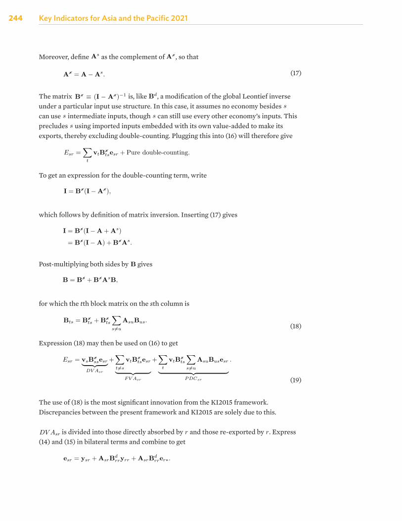
244 Key Indicators for Asia and the Pacific 2021
Moreover, define
example with s = C,
AC =
ACC 0 0AJC AJJ AJU
AUC AUJ AUU
.
Moreover, define As as the complement of As , so that
As = A − As. (17)
The matrix Bs ≡ (I − As)−1 is, like Bd, a modification of the global Leontief inverse under a particularinput use structure. In this case, it assumes no economy besides s can use s intermediate inputs, though s
can still use every other economy’s inputs. This precludes s using imported inputs embedded with its ownvalue-added to make its exports, thereby excluding double-counting. Plugging this into (16) will thereforegive
Esr =
t
vtBstsesr + Pure double-counting.
To get an expression for the double-counting term, write
I = Bs(I − As),
which follows by definition of matrix inversion. Inserting (17) gives
I = Bs(I − A + As)
= Bs(I − A) + BsAs.
Post-multiplying both sides by B gives
B = Bs + BsAsB,
for which the tth block matrix on the sth column is
Bts = Bsts + Bs
ts
s=u
AsuBus. (18)
Expression (18) may then be used on (16) to get
Esr = vsBsssesr
DV Asr
+t=s
vtBstsesr
F V Asr
+
t
vtBsts
s=u
AsuBusesr
P DCsr
. (19)
The use of (18) is the most significant innovation from the KI2015 framework. Discrepancies between thepresent framework and KI2015 are solely due to this.
DV Asr is divided into those directly absorbed by r and those re-exported by r. Express (14) and (15) in
7
as the complement of
example with s = C,
AC =
ACC 0 0AJC AJJ AJU
AUC AUJ AUU
.
Moreover, define As as the complement of As , so that
As = A − As. (17)
The matrix Bs ≡ (I − As)−1 is, like Bd, a modification of the global Leontief inverse under a particularinput use structure. In this case, it assumes no economy besides s can use s intermediate inputs, though s
can still use every other economy’s inputs. This precludes s using imported inputs embedded with its ownvalue-added to make its exports, thereby excluding double-counting. Plugging this into (16) will thereforegive
Esr =
t
vtBstsesr + Pure double-counting.
To get an expression for the double-counting term, write
I = Bs(I − As),
which follows by definition of matrix inversion. Inserting (17) gives
I = Bs(I − A + As)
= Bs(I − A) + BsAs.
Post-multiplying both sides by B gives
B = Bs + BsAsB,
for which the tth block matrix on the sth column is
Bts = Bsts + Bs
ts
s=u
AsuBus. (18)
Expression (18) may then be used on (16) to get
Esr = vsBsssesr
DV Asr
+t=s
vtBstsesr
F V Asr
+
t
vtBsts
s=u
AsuBusesr
P DCsr
. (19)
The use of (18) is the most significant innovation from the KI2015 framework. Discrepancies between thepresent framework and KI2015 are solely due to this.
DV Asr is divided into those directly absorbed by r and those re-exported by r. Express (14) and (15) in
7
, so that
example with s = C,
AC =
ACC 0 0AJC AJJ AJU
AUC AUJ AUU
.
Moreover, define As as the complement of As , so that
As = A − As. (17)
The matrix Bs ≡ (I − As)−1 is, like Bd, a modification of the global Leontief inverse under a particularinput use structure. In this case, it assumes no economy besides s can use s intermediate inputs, though s
can still use every other economy’s inputs. This precludes s using imported inputs embedded with its ownvalue-added to make its exports, thereby excluding double-counting. Plugging this into (16) will thereforegive
Esr =
t
vtBstsesr + Pure double-counting.
To get an expression for the double-counting term, write
I = Bs(I − As),
which follows by definition of matrix inversion. Inserting (17) gives
I = Bs(I − A + As)
= Bs(I − A) + BsAs.
Post-multiplying both sides by B gives
B = Bs + BsAsB,
for which the tth block matrix on the sth column is
Bts = Bsts + Bs
ts
s=u
AsuBus. (18)
Expression (18) may then be used on (16) to get
Esr = vsBsssesr
DV Asr
+t=s
vtBstsesr
F V Asr
+
t
vtBsts
s=u
AsuBusesr
P DCsr
. (19)
The use of (18) is the most significant innovation from the KI2015 framework. Discrepancies between thepresent framework and KI2015 are solely due to this.
DV Asr is divided into those directly absorbed by r and those re-exported by r. Express (14) and (15) in
7
(17)
The matrix
example with s = C,
AC =
ACC 0 0AJC AJJ AJU
AUC AUJ AUU
.
Moreover, define As as the complement of As , so that
As = A − As. (17)
The matrix Bs ≡ (I − As)−1 is, like Bd, a modification of the global Leontief inverse under a particularinput use structure. In this case, it assumes no economy besides s can use s intermediate inputs, though s
can still use every other economy’s inputs. This precludes s using imported inputs embedded with its ownvalue-added to make its exports, thereby excluding double-counting. Plugging this into (16) will thereforegive
Esr =
t
vtBstsesr + Pure double-counting.
To get an expression for the double-counting term, write
I = Bs(I − As),
which follows by definition of matrix inversion. Inserting (17) gives
I = Bs(I − A + As)
= Bs(I − A) + BsAs.
Post-multiplying both sides by B gives
B = Bs + BsAsB,
for which the tth block matrix on the sth column is
Bts = Bsts + Bs
ts
s=u
AsuBus. (18)
Expression (18) may then be used on (16) to get
Esr = vsBsssesr
DV Asr
+t=s
vtBstsesr
F V Asr
+
t
vtBsts
s=u
AsuBusesr
P DCsr
. (19)
The use of (18) is the most significant innovation from the KI2015 framework. Discrepancies between thepresent framework and KI2015 are solely due to this.
DV Asr is divided into those directly absorbed by r and those re-exported by r. Express (14) and (15) in
7
is, like
example with s = C,
AC =
ACC 0 0AJC AJJ AJU
AUC AUJ AUU
.
Moreover, define As as the complement of As , so that
As = A − As. (17)
The matrix Bs ≡ (I − As)−1 is, like Bd, a modification of the global Leontief inverse under a particularinput use structure. In this case, it assumes no economy besides s can use s intermediate inputs, though s
can still use every other economy’s inputs. This precludes s using imported inputs embedded with its ownvalue-added to make its exports, thereby excluding double-counting. Plugging this into (16) will thereforegive
Esr =
t
vtBstsesr + Pure double-counting.
To get an expression for the double-counting term, write
I = Bs(I − As),
which follows by definition of matrix inversion. Inserting (17) gives
I = Bs(I − A + As)
= Bs(I − A) + BsAs.
Post-multiplying both sides by B gives
B = Bs + BsAsB,
for which the tth block matrix on the sth column is
Bts = Bsts + Bs
ts
s=u
AsuBus. (18)
Expression (18) may then be used on (16) to get
Esr = vsBsssesr
DV Asr
+t=s
vtBstsesr
F V Asr
+
t
vtBsts
s=u
AsuBusesr
P DCsr
. (19)
The use of (18) is the most significant innovation from the KI2015 framework. Discrepancies between thepresent framework and KI2015 are solely due to this.
DV Asr is divided into those directly absorbed by r and those re-exported by r. Express (14) and (15) in
7
, a modification of the global Leontief inverse under a particular input use structure. In this case, it assumes no economy besides
element v(s,i) ≡ va(s,i)/x(s,i). This gives the value-added-to-output ratio for each economy–sector. It followsthat
∑(s,j) a(s,j),(r,i) + v(r,i) = 1. Premultiplying this to (11) converts everything to value-added terms:
vsxs ≡ vas = vs
G∑r
G∑u
Bsryru. (12)
Note that this ends up summing sector-level quantities into the aggregate level. To prevent this, see thesection on sector breakdowns.
This expression gives the value-added generated in economy s that is eventually consumed in economy u.It can be tweaked to measure other flows. For example, vsBsryru considers s value-added embodied infinal goods completed in r that are sold to u. To measure s value-added embodied in r’s total exports, onemay instead write vsBsrer∗. These expressions are called VB decompositions and they serve to identify thevalue-added origins of certain quantities.
Even more specific flows may be derived by defining input use structures for domestic intermediates Zd andforeign intermediates Zf separately, yielding Ad and Af where A = Ad +Af . Equation (8) can be rewrittenas
x = (Adx + yd) + (Af x + yf ). (13)
Moreover, since Zf i = Af x, the exports vector (6) can also be rewritten as
e = Af x + yf . (14)
Plugging this into (13) and solving for x,
x = (Adx + yd) + e
= (I − Ad)−1(yd + e)
= Bd(yd + e). (15)
The matrix Bd is called the local Leontief inverse matrix. Its interpretation is the same as the B matrix,except it assumes an input structure that precludes buying and selling inputs abroad. As such, only theblock diagonal elements are non-zero. This isolates the purely domestic portion of production. ComparevsBssyss and vsBd
ssyss. While they both meaure s value-added in its own final consumption, the firstexpression allows for some processing abroad while the second restricts it to purely domestic linkages. Thiswill be crucial in disentangling direct and indirect trading.
Decomposing Exports into Value-Added Categories
Gross exports mask several distinct forms of trading. A substantial portion for most economies is directtrading, where value-added crosses one border before being consumed. The rest involves indirect trading,which itself can take three forms. It can arise from the use of imported inputs, so that one economy’s exportscontain value-added from another economy. It can arise from re-exports, so that one economy’s value-addedgets absorbed somewhere other than its direct importer. Finally, it can arise from what is called “pure”
5
can use
element v(s,i) ≡ va(s,i)/x(s,i). This gives the value-added-to-output ratio for each economy–sector. It followsthat
∑(s,j) a(s,j),(r,i) + v(r,i) = 1. Premultiplying this to (11) converts everything to value-added terms:
vsxs ≡ vas = vs
G∑r
G∑u
Bsryru. (12)
Note that this ends up summing sector-level quantities into the aggregate level. To prevent this, see thesection on sector breakdowns.
This expression gives the value-added generated in economy s that is eventually consumed in economy u.It can be tweaked to measure other flows. For example, vsBsryru considers s value-added embodied infinal goods completed in r that are sold to u. To measure s value-added embodied in r’s total exports, onemay instead write vsBsrer∗. These expressions are called VB decompositions and they serve to identify thevalue-added origins of certain quantities.
Even more specific flows may be derived by defining input use structures for domestic intermediates Zd andforeign intermediates Zf separately, yielding Ad and Af where A = Ad +Af . Equation (8) can be rewrittenas
x = (Adx + yd) + (Af x + yf ). (13)
Moreover, since Zf i = Af x, the exports vector (6) can also be rewritten as
e = Af x + yf . (14)
Plugging this into (13) and solving for x,
x = (Adx + yd) + e
= (I − Ad)−1(yd + e)
= Bd(yd + e). (15)
The matrix Bd is called the local Leontief inverse matrix. Its interpretation is the same as the B matrix,except it assumes an input structure that precludes buying and selling inputs abroad. As such, only theblock diagonal elements are non-zero. This isolates the purely domestic portion of production. ComparevsBssyss and vsBd
ssyss. While they both meaure s value-added in its own final consumption, the firstexpression allows for some processing abroad while the second restricts it to purely domestic linkages. Thiswill be crucial in disentangling direct and indirect trading.
Decomposing Exports into Value-Added Categories
Gross exports mask several distinct forms of trading. A substantial portion for most economies is directtrading, where value-added crosses one border before being consumed. The rest involves indirect trading,which itself can take three forms. It can arise from the use of imported inputs, so that one economy’s exportscontain value-added from another economy. It can arise from re-exports, so that one economy’s value-addedgets absorbed somewhere other than its direct importer. Finally, it can arise from what is called “pure”
5
intermediate inputs, though
element v(s,i) ≡ va(s,i)/x(s,i). This gives the value-added-to-output ratio for each economy–sector. It followsthat
∑(s,j) a(s,j),(r,i) + v(r,i) = 1. Premultiplying this to (11) converts everything to value-added terms:
vsxs ≡ vas = vs
G∑r
G∑u
Bsryru. (12)
Note that this ends up summing sector-level quantities into the aggregate level. To prevent this, see thesection on sector breakdowns.
This expression gives the value-added generated in economy s that is eventually consumed in economy u.It can be tweaked to measure other flows. For example, vsBsryru considers s value-added embodied infinal goods completed in r that are sold to u. To measure s value-added embodied in r’s total exports, onemay instead write vsBsrer∗. These expressions are called VB decompositions and they serve to identify thevalue-added origins of certain quantities.
Even more specific flows may be derived by defining input use structures for domestic intermediates Zd andforeign intermediates Zf separately, yielding Ad and Af where A = Ad +Af . Equation (8) can be rewrittenas
x = (Adx + yd) + (Af x + yf ). (13)
Moreover, since Zf i = Af x, the exports vector (6) can also be rewritten as
e = Af x + yf . (14)
Plugging this into (13) and solving for x,
x = (Adx + yd) + e
= (I − Ad)−1(yd + e)
= Bd(yd + e). (15)
The matrix Bd is called the local Leontief inverse matrix. Its interpretation is the same as the B matrix,except it assumes an input structure that precludes buying and selling inputs abroad. As such, only theblock diagonal elements are non-zero. This isolates the purely domestic portion of production. ComparevsBssyss and vsBd
ssyss. While they both meaure s value-added in its own final consumption, the firstexpression allows for some processing abroad while the second restricts it to purely domestic linkages. Thiswill be crucial in disentangling direct and indirect trading.
Decomposing Exports into Value-Added Categories
Gross exports mask several distinct forms of trading. A substantial portion for most economies is directtrading, where value-added crosses one border before being consumed. The rest involves indirect trading,which itself can take three forms. It can arise from the use of imported inputs, so that one economy’s exportscontain value-added from another economy. It can arise from re-exports, so that one economy’s value-addedgets absorbed somewhere other than its direct importer. Finally, it can arise from what is called “pure”
5
can still use every other economy’s inputs. This precludes
element v(s,i) ≡ va(s,i)/x(s,i). This gives the value-added-to-output ratio for each economy–sector. It followsthat
∑(s,j) a(s,j),(r,i) + v(r,i) = 1. Premultiplying this to (11) converts everything to value-added terms:
vsxs ≡ vas = vs
G∑r
G∑u
Bsryru. (12)
Note that this ends up summing sector-level quantities into the aggregate level. To prevent this, see thesection on sector breakdowns.
This expression gives the value-added generated in economy s that is eventually consumed in economy u.It can be tweaked to measure other flows. For example, vsBsryru considers s value-added embodied infinal goods completed in r that are sold to u. To measure s value-added embodied in r’s total exports, onemay instead write vsBsrer∗. These expressions are called VB decompositions and they serve to identify thevalue-added origins of certain quantities.
Even more specific flows may be derived by defining input use structures for domestic intermediates Zd andforeign intermediates Zf separately, yielding Ad and Af where A = Ad +Af . Equation (8) can be rewrittenas
x = (Adx + yd) + (Af x + yf ). (13)
Moreover, since Zf i = Af x, the exports vector (6) can also be rewritten as
e = Af x + yf . (14)
Plugging this into (13) and solving for x,
x = (Adx + yd) + e
= (I − Ad)−1(yd + e)
= Bd(yd + e). (15)
The matrix Bd is called the local Leontief inverse matrix. Its interpretation is the same as the B matrix,except it assumes an input structure that precludes buying and selling inputs abroad. As such, only theblock diagonal elements are non-zero. This isolates the purely domestic portion of production. ComparevsBssyss and vsBd
ssyss. While they both meaure s value-added in its own final consumption, the firstexpression allows for some processing abroad while the second restricts it to purely domestic linkages. Thiswill be crucial in disentangling direct and indirect trading.
Decomposing Exports into Value-Added Categories
Gross exports mask several distinct forms of trading. A substantial portion for most economies is directtrading, where value-added crosses one border before being consumed. The rest involves indirect trading,which itself can take three forms. It can arise from the use of imported inputs, so that one economy’s exportscontain value-added from another economy. It can arise from re-exports, so that one economy’s value-addedgets absorbed somewhere other than its direct importer. Finally, it can arise from what is called “pure”
5
using imported inputs embedded with its own value-added to make its exports, thereby excluding double-counting. Plugging this into (16) will therefore give
example with s = C,
AC =
ACC 0 0AJC AJJ AJU
AUC AUJ AUU
.
Moreover, define As as the complement of As , so that
As = A − As. (17)
The matrix Bs ≡ (I − As)−1 is, like Bd, a modification of the global Leontief inverse under a particularinput use structure. In this case, it assumes no economy besides s can use s intermediate inputs, though s
can still use every other economy’s inputs. This precludes s using imported inputs embedded with its ownvalue-added to make its exports, thereby excluding double-counting. Plugging this into (16) will thereforegive
Esr =
t
vtBstsesr + Pure double-counting.
To get an expression for the double-counting term, write
I = Bs(I − As),
which follows by definition of matrix inversion. Inserting (17) gives
I = Bs(I − A + As)
= Bs(I − A) + BsAs.
Post-multiplying both sides by B gives
B = Bs + BsAsB,
for which the tth block matrix on the sth column is
Bts = Bsts + Bs
ts
s=u
AsuBus. (18)
Expression (18) may then be used on (16) to get
Esr = vsBsssesr
DV Asr
+t=s
vtBstsesr
F V Asr
+
t
vtBsts
s=u
AsuBusesr
P DCsr
. (19)
The use of (18) is the most significant innovation from the KI2015 framework. Discrepancies between thepresent framework and KI2015 are solely due to this.
DV Asr is divided into those directly absorbed by r and those re-exported by r. Express (14) and (15) in
7
To get an expression for the double-counting term, write
example with s = C,
AC =
ACC 0 0AJC AJJ AJU
AUC AUJ AUU
.
Moreover, define As as the complement of As , so that
As = A − As. (17)
The matrix Bs ≡ (I − As)−1 is, like Bd, a modification of the global Leontief inverse under a particularinput use structure. In this case, it assumes no economy besides s can use s intermediate inputs, though s
can still use every other economy’s inputs. This precludes s using imported inputs embedded with its ownvalue-added to make its exports, thereby excluding double-counting. Plugging this into (16) will thereforegive
Esr =
t
vtBstsesr + Pure double-counting.
To get an expression for the double-counting term, write
I = Bs(I − As),
which follows by definition of matrix inversion. Inserting (17) gives
I = Bs(I − A + As)
= Bs(I − A) + BsAs.
Post-multiplying both sides by B gives
B = Bs + BsAsB,
for which the tth block matrix on the sth column is
Bts = Bsts + Bs
ts
s=u
AsuBus. (18)
Expression (18) may then be used on (16) to get
Esr = vsBsssesr
DV Asr
+t=s
vtBstsesr
F V Asr
+
t
vtBsts
s=u
AsuBusesr
P DCsr
. (19)
The use of (18) is the most significant innovation from the KI2015 framework. Discrepancies between thepresent framework and KI2015 are solely due to this.
DV Asr is divided into those directly absorbed by r and those re-exported by r. Express (14) and (15) in
7
which follows by definition of matrix inversion. Inserting (17) gives
example with s = C,
AC =
ACC 0 0AJC AJJ AJU
AUC AUJ AUU
.
Moreover, define As as the complement of As , so that
As = A − As. (17)
The matrix Bs ≡ (I − As)−1 is, like Bd, a modification of the global Leontief inverse under a particularinput use structure. In this case, it assumes no economy besides s can use s intermediate inputs, though s
can still use every other economy’s inputs. This precludes s using imported inputs embedded with its ownvalue-added to make its exports, thereby excluding double-counting. Plugging this into (16) will thereforegive
Esr =
t
vtBstsesr + Pure double-counting.
To get an expression for the double-counting term, write
I = Bs(I − As),
which follows by definition of matrix inversion. Inserting (17) gives
I = Bs(I − A + As)
= Bs(I − A) + BsAs.
Post-multiplying both sides by B gives
B = Bs + BsAsB,
for which the tth block matrix on the sth column is
Bts = Bsts + Bs
ts
s=u
AsuBus. (18)
Expression (18) may then be used on (16) to get
Esr = vsBsssesr
DV Asr
+t=s
vtBstsesr
F V Asr
+
t
vtBsts
s=u
AsuBusesr
P DCsr
. (19)
The use of (18) is the most significant innovation from the KI2015 framework. Discrepancies between thepresent framework and KI2015 are solely due to this.
DV Asr is divided into those directly absorbed by r and those re-exported by r. Express (14) and (15) in
7
Post-multiplying both sides by
example with s = C,
AC =
ACC 0 0AJC AJJ AJU
AUC AUJ AUU
.
Moreover, define As as the complement of As , so that
As = A − As. (17)
The matrix Bs ≡ (I − As)−1 is, like Bd, a modification of the global Leontief inverse under a particularinput use structure. In this case, it assumes no economy besides s can use s intermediate inputs, though s
can still use every other economy’s inputs. This precludes s using imported inputs embedded with its ownvalue-added to make its exports, thereby excluding double-counting. Plugging this into (16) will thereforegive
Esr =
t
vtBstsesr + Pure double-counting.
To get an expression for the double-counting term, write
I = Bs(I − As),
which follows by definition of matrix inversion. Inserting (17) gives
I = Bs(I − A + As)
= Bs(I − A) + BsAs.
Post-multiplying both sides by B gives
B = Bs + BsAsB,
for which the tth block matrix on the sth column is
Bts = Bsts + Bs
ts
s=u
AsuBus. (18)
Expression (18) may then be used on (16) to get
Esr = vsBsssesr
DV Asr
+t=s
vtBstsesr
F V Asr
+
t
vtBsts
s=u
AsuBusesr
P DCsr
. (19)
The use of (18) is the most significant innovation from the KI2015 framework. Discrepancies between thepresent framework and KI2015 are solely due to this.
DV Asr is divided into those directly absorbed by r and those re-exported by r. Express (14) and (15) in
7
gives
example with s = C,
AC =
ACC 0 0AJC AJJ AJU
AUC AUJ AUU
.
Moreover, define As as the complement of As , so that
As = A − As. (17)
The matrix Bs ≡ (I − As)−1 is, like Bd, a modification of the global Leontief inverse under a particularinput use structure. In this case, it assumes no economy besides s can use s intermediate inputs, though s
can still use every other economy’s inputs. This precludes s using imported inputs embedded with its ownvalue-added to make its exports, thereby excluding double-counting. Plugging this into (16) will thereforegive
Esr =
t
vtBstsesr + Pure double-counting.
To get an expression for the double-counting term, write
I = Bs(I − As),
which follows by definition of matrix inversion. Inserting (17) gives
I = Bs(I − A + As)
= Bs(I − A) + BsAs.
Post-multiplying both sides by B gives
B = Bs + BsAsB,
for which the tth block matrix on the sth column is
Bts = Bsts + Bs
ts
s=u
AsuBus. (18)
Expression (18) may then be used on (16) to get
Esr = vsBsssesr
DV Asr
+t=s
vtBstsesr
F V Asr
+
t
vtBsts
s=u
AsuBusesr
P DCsr
. (19)
The use of (18) is the most significant innovation from the KI2015 framework. Discrepancies between thepresent framework and KI2015 are solely due to this.
DV Asr is divided into those directly absorbed by r and those re-exported by r. Express (14) and (15) in
7
for which the tth block matrix on the sth column is
example with s = C,
AC =
ACC 0 0AJC AJJ AJU
AUC AUJ AUU
.
Moreover, define As as the complement of As , so that
As = A − As. (17)
The matrix Bs ≡ (I − As)−1 is, like Bd, a modification of the global Leontief inverse under a particularinput use structure. In this case, it assumes no economy besides s can use s intermediate inputs, though s
can still use every other economy’s inputs. This precludes s using imported inputs embedded with its ownvalue-added to make its exports, thereby excluding double-counting. Plugging this into (16) will thereforegive
Esr =
t
vtBstsesr + Pure double-counting.
To get an expression for the double-counting term, write
I = Bs(I − As),
which follows by definition of matrix inversion. Inserting (17) gives
I = Bs(I − A + As)
= Bs(I − A) + BsAs.
Post-multiplying both sides by B gives
B = Bs + BsAsB,
for which the tth block matrix on the sth column is
Bts = Bsts + Bs
ts
s =u
AsuBus. (18)
Expression (18) may then be used on (16) to get
Esr = vsBsssesr
DV Asr
+t=s
vtBstsesr
F V Asr
+
t
vtBsts
s=u
AsuBusesr
P DCsr
. (19)
The use of (18) is the most significant innovation from the KI2015 framework. Discrepancies between thepresent framework and KI2015 are solely due to this.
DV Asr is divided into those directly absorbed by r and those re-exported by r. Express (14) and (15) in
7
(18)
Expression (18) may then be used on (16) to get
example with s = C,
AC =
ACC 0 0AJC AJJ AJU
AUC AUJ AUU
.
Moreover, define As as the complement of As , so that
As = A − As. (17)
The matrix Bs ≡ (I − As)−1 is, like Bd, a modification of the global Leontief inverse under a particularinput use structure. In this case, it assumes no economy besides s can use s intermediate inputs, though s
can still use every other economy’s inputs. This precludes s using imported inputs embedded with its ownvalue-added to make its exports, thereby excluding double-counting. Plugging this into (16) will thereforegive
Esr =
t
vtBstsesr + Pure double-counting.
To get an expression for the double-counting term, write
I = Bs(I − As),
which follows by definition of matrix inversion. Inserting (17) gives
I = Bs(I − A + As)
= Bs(I − A) + BsAs.
Post-multiplying both sides by B gives
B = Bs + BsAsB,
for which the tth block matrix on the sth column is
Bts = Bsts + Bs
ts
s=u
AsuBus. (18)
Expression (18) may then be used on (16) to get
Esr = vsBsssesr
DV Asr
+t=s
vtBstsesr
F V Asr
+
t
vtBsts
s=u
AsuBusesr
P DCsr
. (19)
The use of (18) is the most significant innovation from the KI2015 framework. Discrepancies between thepresent framework and KI2015 are solely due to this.
DV Asr is divided into those directly absorbed by r and those re-exported by r. Express (14) and (15) in
7
(19)
The use of (18) is the most significant innovation from the KI2015 framework. Discrepancies between the present framework and KI2015 are solely due to this.
example with s = C,
AC =
ACC 0 0AJC AJJ AJU
AUC AUJ AUU
.
Moreover, define As as the complement of As , so that
As = A − As. (17)
The matrix Bs ≡ (I − As)−1 is, like Bd, a modification of the global Leontief inverse under a particularinput use structure. In this case, it assumes no economy besides s can use s intermediate inputs, though s
can still use every other economy’s inputs. This precludes s using imported inputs embedded with its ownvalue-added to make its exports, thereby excluding double-counting. Plugging this into (16) will thereforegive
Esr =
t
vtBstsesr + Pure double-counting.
To get an expression for the double-counting term, write
I = Bs(I − As),
which follows by definition of matrix inversion. Inserting (17) gives
I = Bs(I − A + As)
= Bs(I − A) + BsAs.
Post-multiplying both sides by B gives
B = Bs + BsAsB,
for which the tth block matrix on the sth column is
Bts = Bsts + Bs
ts
s=u
AsuBus. (18)
Expression (18) may then be used on (16) to get
Esr = vsBsssesr
DV Asr
+t=s
vtBstsesr
F V Asr
+
t
vtBsts
s=u
AsuBusesr
P DCsr
. (19)
The use of (18) is the most significant innovation from the KI2015 framework. Discrepancies between thepresent framework and KI2015 are solely due to this.
DV Asr is divided into those directly absorbed by r and those re-exported by r. Express (14) and (15) in
7
is divided into those directly absorbed by
where ⊗ denote a Kronecker product. Written out,
E ≡
0 zC1,J1 + zC1,J2 zC1,U1 + zC1,U2
0 zC2,J1 + zC2,J2 zC2,U1 + zC2,U2
zJ1,C1 + zJ1,C2 0 zJ1,U1 + zJ1,U2
zJ2,C1 + zJ2,C2 0 zJ2,U1 + zJ2,U2
zU1,C1 + zU1,C2 zU1,J1 + zU1,J2 0zU2,C1 + zU2,C2 zU2,J1 + zU2,J2 0
+
0 yC1,J yC1,U
0 yC2,J yC2,U
yJ1,C 0 yJ1,U
yJ2,C 0 yJ2,U
yU1,C yU1,J 0yU2,C yU2,J 0
=
0 eC1,J eC1,U
0 eC2,J eC2,U
eJ1,C 0 eJ1,U
eJ2,C 0 eJ2,U
eU1,C eU1,J 0eU2,C eU2,J 0
=
0 eCJ eCU
eJC 0 eJU
eUC eUJ 0
The technical coefficient a(s,j),(r,i) is the share of inputs from (s, j) in the output of (r, i): a(s,j),(r,i) ≡z(s,j),(r,i)/x(r,i). Collect all these into the GN × GN matrix of technical coefficients A. This may be used torewrite (3) as
x = Ax + y. (8)
Solving for x gives
x = (I − A)−1y = By, (9)
where the GN × GN matrix B is called the global Leontief inverse matrix.
VB Decomposition
Equation (9) is central to analyzing cross-economy and cross-sectoral linkages. It is clearer to see this if (8)and (9) are rewritten to isolate a single economy s:
xs =Gr
Asrxr +Gr
ysr (10)
=Gr
Gu
Bsryru (11)
Equation (10) says that s’s output xs is used as intermediates in r’s output or sold as final goods to r (for allr = 1, ..., G). The output of each r can in turn be used as intermediates by other economies, whose outputsare then used by further economies, and so on in a potentially infinite series of production stages. Equation(11) summarizes these to identify the final landing stage of s’s output. The product Bsryru is s output thatis “completed” into a final good by r, which then sends it to u for final absorption.
In most analyses, value-added rather than output is the preferred metric. Define the vector v with (s, i)th
4
and those re-exported by
where ⊗ denote a Kronecker product. Written out,
E ≡
0 zC1,J1 + zC1,J2 zC1,U1 + zC1,U2
0 zC2,J1 + zC2,J2 zC2,U1 + zC2,U2
zJ1,C1 + zJ1,C2 0 zJ1,U1 + zJ1,U2
zJ2,C1 + zJ2,C2 0 zJ2,U1 + zJ2,U2
zU1,C1 + zU1,C2 zU1,J1 + zU1,J2 0zU2,C1 + zU2,C2 zU2,J1 + zU2,J2 0
+
0 yC1,J yC1,U
0 yC2,J yC2,U
yJ1,C 0 yJ1,U
yJ2,C 0 yJ2,U
yU1,C yU1,J 0yU2,C yU2,J 0
=
0 eC1,J eC1,U
0 eC2,J eC2,U
eJ1,C 0 eJ1,U
eJ2,C 0 eJ2,U
eU1,C eU1,J 0eU2,C eU2,J 0
=
0 eCJ eCU
eJC 0 eJU
eUC eUJ 0
The technical coefficient a(s,j),(r,i) is the share of inputs from (s, j) in the output of (r, i): a(s,j),(r,i) ≡z(s,j),(r,i)/x(r,i). Collect all these into the GN × GN matrix of technical coefficients A. This may be used torewrite (3) as
x = Ax + y. (8)
Solving for x gives
x = (I − A)−1y = By, (9)
where the GN × GN matrix B is called the global Leontief inverse matrix.
VB Decomposition
Equation (9) is central to analyzing cross-economy and cross-sectoral linkages. It is clearer to see this if (8)and (9) are rewritten to isolate a single economy s:
xs =Gr
Asrxr +Gr
ysr (10)
=Gr
Gu
Bsryru (11)
Equation (10) says that s’s output xs is used as intermediates in r’s output or sold as final goods to r (for allr = 1, ..., G). The output of each r can in turn be used as intermediates by other economies, whose outputsare then used by further economies, and so on in a potentially infinite series of production stages. Equation(11) summarizes these to identify the final landing stage of s’s output. The product Bsryru is s output thatis “completed” into a final good by r, which then sends it to u for final absorption.
In most analyses, value-added rather than output is the preferred metric. Define the vector v with (s, i)th
4
. Express (14) and (15) in bilateral terms and combine to get
bilateral terms and combine to get
esr = ysr + AsrBdrryrr + AsrBd
rrer∗.
This simply states that all exports to r must either be final goods consumed by r or intermediates used byr. Output in the latter may in turn be absorbed by r or re-exported and absorbed elsewhere. Using this toexpand DV Asr gives
DV Asr = vsBsss
[ysr + AsrBd
rryrr + AsrBdrrer∗
].
The first two terms comprise exports to r that are absorbed in r without passing through any other border.These are termed “directly absorbed value-added exports” or DAV AX. Economy r’s re-exports, AsrBd
rrer∗,may be broken down into those that ultimately end up back in economy s, called “reflection” (REF ) followingKoopman, Wang, and Wei (2014), and those that end up elsewhere (REX). It is also helpful to extractfrom the latter those that are ultimately absorbed by the direct importer r.
DV Asr = vsBsss
[ysr + AsrBd
rryrr
]︸ ︷︷ ︸
DAV AXsr
+ vsBsssAsrBd
rr
[ ∑u=r,s
yru +∑u=r
Aru
( ∑k
∑ℓ=s,r
Bukykℓ +∑
k
Bukykr
)]
︸ ︷︷ ︸REXsr
(20)
+ vsBsssAsrBd
rr
[yrs +
∑u=r
Aru
∑k
Bukyks
]
︸ ︷︷ ︸REF sr
.
Each term has two or more sub-terms, referred to sequentially as DAV AX1, DAV AX2, and so on. Thisdecomposition may also be done on FV A but is omitted here.
Equations (19) and (20) comprise the value-added trade accounting framework.4 A full description of eachterm is given in Table A3.1.1, along with their counterparts, if any, to KI2015.5 Overall, the presentframework streamlines KI2015’s 16 terms into 5 broad categories: DAV AX, REX, REF , FV A, and PDC.These may be elaborated into 10 finer categories.
Sector Breakdowns
Equations (19) and (20) yield aggregate, economy-wide figures, thought oftentimes the analysis requires amore granular, sector-level perspective. Borin and Mancini (2019) gave three main approaches to breakingdown aggregate figures by sector.6
4In Borin and Mancini’s (2019) taxonomy of trade accounting frameworks, this is a source-based approach from the exporter’sperspective.
5Note that this is only a conceptual correspondence, meaning they intend to measure the same thing. Most terms, however,cannot mathematically be reconciled with those in KI2015 due to the use of (18). Note also that REX1, REX2, and REX3have no counterparts in KI2015, though their sum conceptually corresponds to the sum of terms 3, 4, and 5.
6In KI2015, breakdown by export sectors is called “backward-linkage-based” while breakdown by origin sectors is called“forward-linkage-based”. See pp. 393–95 of that publication.
8
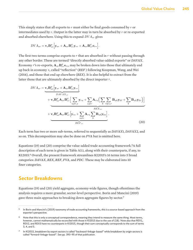
Global Value Chains
245Global Value Chains
This simply states that all exports to
where ⊗ denote a Kronecker product. Written out,
E ≡
0 zC1,J1 + zC1,J2 zC1,U1 + zC1,U2
0 zC2,J1 + zC2,J2 zC2,U1 + zC2,U2
zJ1,C1 + zJ1,C2 0 zJ1,U1 + zJ1,U2
zJ2,C1 + zJ2,C2 0 zJ2,U1 + zJ2,U2
zU1,C1 + zU1,C2 zU1,J1 + zU1,J2 0zU2,C1 + zU2,C2 zU2,J1 + zU2,J2 0
+
0 yC1,J yC1,U
0 yC2,J yC2,U
yJ1,C 0 yJ1,U
yJ2,C 0 yJ2,U
yU1,C yU1,J 0yU2,C yU2,J 0
=
0 eC1,J eC1,U
0 eC2,J eC2,U
eJ1,C 0 eJ1,U
eJ2,C 0 eJ2,U
eU1,C eU1,J 0eU2,C eU2,J 0
=
0 eCJ eCU
eJC 0 eJU
eUC eUJ 0
The technical coefficient a(s,j),(r,i) is the share of inputs from (s, j) in the output of (r, i): a(s,j),(r,i) ≡z(s,j),(r,i)/x(r,i). Collect all these into the GN × GN matrix of technical coefficients A. This may be used torewrite (3) as
x = Ax + y. (8)
Solving for x gives
x = (I − A)−1y = By, (9)
where the GN × GN matrix B is called the global Leontief inverse matrix.
VB Decomposition
Equation (9) is central to analyzing cross-economy and cross-sectoral linkages. It is clearer to see this if (8)and (9) are rewritten to isolate a single economy s:
xs =Gr
Asrxr +Gr
ysr (10)
=Gr
Gu
Bsryru (11)
Equation (10) says that s’s output xs is used as intermediates in r’s output or sold as final goods to r (for allr = 1, ..., G). The output of each r can in turn be used as intermediates by other economies, whose outputsare then used by further economies, and so on in a potentially infinite series of production stages. Equation(11) summarizes these to identify the final landing stage of s’s output. The product Bsryru is s output thatis “completed” into a final good by r, which then sends it to u for final absorption.
In most analyses, value-added rather than output is the preferred metric. Define the vector v with (s, i)th
4
must either be final goods consumed by
where ⊗ denote a Kronecker product. Written out,
E ≡
0 zC1,J1 + zC1,J2 zC1,U1 + zC1,U2
0 zC2,J1 + zC2,J2 zC2,U1 + zC2,U2
zJ1,C1 + zJ1,C2 0 zJ1,U1 + zJ1,U2
zJ2,C1 + zJ2,C2 0 zJ2,U1 + zJ2,U2
zU1,C1 + zU1,C2 zU1,J1 + zU1,J2 0zU2,C1 + zU2,C2 zU2,J1 + zU2,J2 0
+
0 yC1,J yC1,U
0 yC2,J yC2,U
yJ1,C 0 yJ1,U
yJ2,C 0 yJ2,U
yU1,C yU1,J 0yU2,C yU2,J 0
=
0 eC1,J eC1,U
0 eC2,J eC2,U
eJ1,C 0 eJ1,U
eJ2,C 0 eJ2,U
eU1,C eU1,J 0eU2,C eU2,J 0
=
0 eCJ eCU
eJC 0 eJU
eUC eUJ 0
The technical coefficient a(s,j),(r,i) is the share of inputs from (s, j) in the output of (r, i): a(s,j),(r,i) ≡z(s,j),(r,i)/x(r,i). Collect all these into the GN × GN matrix of technical coefficients A. This may be used torewrite (3) as
x = Ax + y. (8)
Solving for x gives
x = (I − A)−1y = By, (9)
where the GN × GN matrix B is called the global Leontief inverse matrix.
VB Decomposition
Equation (9) is central to analyzing cross-economy and cross-sectoral linkages. It is clearer to see this if (8)and (9) are rewritten to isolate a single economy s:
xs =Gr
Asrxr +Gr
ysr (10)
=Gr
Gu
Bsryru (11)
Equation (10) says that s’s output xs is used as intermediates in r’s output or sold as final goods to r (for allr = 1, ..., G). The output of each r can in turn be used as intermediates by other economies, whose outputsare then used by further economies, and so on in a potentially infinite series of production stages. Equation(11) summarizes these to identify the final landing stage of s’s output. The product Bsryru is s output thatis “completed” into a final good by r, which then sends it to u for final absorption.
In most analyses, value-added rather than output is the preferred metric. Define the vector v with (s, i)th
4
or intermediates used by
where ⊗ denote a Kronecker product. Written out,
E ≡
0 zC1,J1 + zC1,J2 zC1,U1 + zC1,U2
0 zC2,J1 + zC2,J2 zC2,U1 + zC2,U2
zJ1,C1 + zJ1,C2 0 zJ1,U1 + zJ1,U2
zJ2,C1 + zJ2,C2 0 zJ2,U1 + zJ2,U2
zU1,C1 + zU1,C2 zU1,J1 + zU1,J2 0zU2,C1 + zU2,C2 zU2,J1 + zU2,J2 0
+
0 yC1,J yC1,U
0 yC2,J yC2,U
yJ1,C 0 yJ1,U
yJ2,C 0 yJ2,U
yU1,C yU1,J 0yU2,C yU2,J 0
=
0 eC1,J eC1,U
0 eC2,J eC2,U
eJ1,C 0 eJ1,U
eJ2,C 0 eJ2,U
eU1,C eU1,J 0eU2,C eU2,J 0
=
0 eCJ eCU
eJC 0 eJU
eUC eUJ 0
The technical coefficient a(s,j),(r,i) is the share of inputs from (s, j) in the output of (r, i): a(s,j),(r,i) ≡z(s,j),(r,i)/x(r,i). Collect all these into the GN × GN matrix of technical coefficients A. This may be used torewrite (3) as
x = Ax + y. (8)
Solving for x gives
x = (I − A)−1y = By, (9)
where the GN × GN matrix B is called the global Leontief inverse matrix.
VB Decomposition
Equation (9) is central to analyzing cross-economy and cross-sectoral linkages. It is clearer to see this if (8)and (9) are rewritten to isolate a single economy s:
xs =Gr
Asrxr +Gr
ysr (10)
=Gr
Gu
Bsryru (11)
Equation (10) says that s’s output xs is used as intermediates in r’s output or sold as final goods to r (for allr = 1, ..., G). The output of each r can in turn be used as intermediates by other economies, whose outputsare then used by further economies, and so on in a potentially infinite series of production stages. Equation(11) summarizes these to identify the final landing stage of s’s output. The product Bsryru is s output thatis “completed” into a final good by r, which then sends it to u for final absorption.
In most analyses, value-added rather than output is the preferred metric. Define the vector v with (s, i)th
4
. Output in the latter may in turn be absorbed by
where ⊗ denote a Kronecker product. Written out,
E ≡
0 zC1,J1 + zC1,J2 zC1,U1 + zC1,U2
0 zC2,J1 + zC2,J2 zC2,U1 + zC2,U2
zJ1,C1 + zJ1,C2 0 zJ1,U1 + zJ1,U2
zJ2,C1 + zJ2,C2 0 zJ2,U1 + zJ2,U2
zU1,C1 + zU1,C2 zU1,J1 + zU1,J2 0zU2,C1 + zU2,C2 zU2,J1 + zU2,J2 0
+
0 yC1,J yC1,U
0 yC2,J yC2,U
yJ1,C 0 yJ1,U
yJ2,C 0 yJ2,U
yU1,C yU1,J 0yU2,C yU2,J 0
=
0 eC1,J eC1,U
0 eC2,J eC2,U
eJ1,C 0 eJ1,U
eJ2,C 0 eJ2,U
eU1,C eU1,J 0eU2,C eU2,J 0
=
0 eCJ eCU
eJC 0 eJU
eUC eUJ 0
The technical coefficient a(s,j),(r,i) is the share of inputs from (s, j) in the output of (r, i): a(s,j),(r,i) ≡z(s,j),(r,i)/x(r,i). Collect all these into the GN × GN matrix of technical coefficients A. This may be used torewrite (3) as
x = Ax + y. (8)
Solving for x gives
x = (I − A)−1y = By, (9)
where the GN × GN matrix B is called the global Leontief inverse matrix.
VB Decomposition
Equation (9) is central to analyzing cross-economy and cross-sectoral linkages. It is clearer to see this if (8)and (9) are rewritten to isolate a single economy s:
xs =Gr
Asrxr +Gr
ysr (10)
=Gr
Gu
Bsryru (11)
Equation (10) says that s’s output xs is used as intermediates in r’s output or sold as final goods to r (for allr = 1, ..., G). The output of each r can in turn be used as intermediates by other economies, whose outputsare then used by further economies, and so on in a potentially infinite series of production stages. Equation(11) summarizes these to identify the final landing stage of s’s output. The product Bsryru is s output thatis “completed” into a final good by r, which then sends it to u for final absorption.
In most analyses, value-added rather than output is the preferred metric. Define the vector v with (s, i)th
4
or re-exported and absorbed elsewhere. Using this to expand
bilateral terms and combine to get
esr = ysr + AsrBdrryrr + AsrBd
rrer∗.
This simply states that all exports to r must either be final goods consumed by r or intermediates used byr. Output in the latter may in turn be absorbed by r or re-exported and absorbed elsewhere. Using this toexpand DV Asr gives
DV Asr = vsBsss
[ysr + AsrBd
rryrr + AsrBdrrer∗
].
The first two terms comprise exports to r that are absorbed in r without passing through any other border.These are termed “directly absorbed value-added exports” or DAV AX. Economy r’s re-exports, AsrBd
rrer∗,may be broken down into those that ultimately end up back in economy s, called “reflection” (REF ) followingKoopman, Wang, and Wei (2014), and those that end up elsewhere (REX). It is also helpful to extractfrom the latter those that are ultimately absorbed by the direct importer r.
DV Asr = vsBsss
[ysr + AsrBd
rryrr
]︸ ︷︷ ︸
DAV AXsr
+ vsBsssAsrBd
rr
[ ∑u=r,s
yru +∑u=r
Aru
( ∑k
∑ℓ=s,r
Bukykℓ +∑
k
Bukykr
)]
︸ ︷︷ ︸REXsr
(20)
+ vsBsssAsrBd
rr
[yrs +
∑u=r
Aru
∑k
Bukyks
]
︸ ︷︷ ︸REF sr
.
Each term has two or more sub-terms, referred to sequentially as DAV AX1, DAV AX2, and so on. Thisdecomposition may also be done on FV A but is omitted here.
Equations (19) and (20) comprise the value-added trade accounting framework.4 A full description of eachterm is given in Table A3.1.1, along with their counterparts, if any, to KI2015.5 Overall, the presentframework streamlines KI2015’s 16 terms into 5 broad categories: DAV AX, REX, REF , FV A, and PDC.These may be elaborated into 10 finer categories.
Sector Breakdowns
Equations (19) and (20) yield aggregate, economy-wide figures, thought oftentimes the analysis requires amore granular, sector-level perspective. Borin and Mancini (2019) gave three main approaches to breakingdown aggregate figures by sector.6
4In Borin and Mancini’s (2019) taxonomy of trade accounting frameworks, this is a source-based approach from the exporter’sperspective.
5Note that this is only a conceptual correspondence, meaning they intend to measure the same thing. Most terms, however,cannot mathematically be reconciled with those in KI2015 due to the use of (18). Note also that REX1, REX2, and REX3have no counterparts in KI2015, though their sum conceptually corresponds to the sum of terms 3, 4, and 5.
6In KI2015, breakdown by export sectors is called “backward-linkage-based” while breakdown by origin sectors is called“forward-linkage-based”. See pp. 393–95 of that publication.
8
gives
bilateral terms and combine to get
esr = ysr + AsrBdrryrr + AsrBd
rrer∗.
This simply states that all exports to r must either be final goods consumed by r or intermediates used byr. Output in the latter may in turn be absorbed by r or re-exported and absorbed elsewhere. Using this toexpand DV Asr gives
DV Asr = vsBsss
[ysr + AsrBd
rryrr + AsrBdrrer∗
].
The first two terms comprise exports to r that are absorbed in r without passing through any other border.These are termed “directly absorbed value-added exports” or DAV AX. Economy r’s re-exports, AsrBd
rrer∗,may be broken down into those that ultimately end up back in economy s, called “reflection” (REF ) followingKoopman, Wang, and Wei (2014), and those that end up elsewhere (REX). It is also helpful to extractfrom the latter those that are ultimately absorbed by the direct importer r.
DV Asr = vsBsss
[ysr + AsrBd
rryrr
]︸ ︷︷ ︸
DAV AXsr
+ vsBsssAsrBd
rr
[ ∑u=r,s
yru +∑u=r
Aru
( ∑k
∑ℓ=s,r
Bukykℓ +∑
k
Bukykr
)]
︸ ︷︷ ︸REXsr
(20)
+ vsBsssAsrBd
rr
[yrs +
∑u=r
Aru
∑k
Bukyks
]
︸ ︷︷ ︸REF sr
.
Each term has two or more sub-terms, referred to sequentially as DAV AX1, DAV AX2, and so on. Thisdecomposition may also be done on FV A but is omitted here.
Equations (19) and (20) comprise the value-added trade accounting framework.4 A full description of eachterm is given in Table A3.1.1, along with their counterparts, if any, to KI2015.5 Overall, the presentframework streamlines KI2015’s 16 terms into 5 broad categories: DAV AX, REX, REF , FV A, and PDC.These may be elaborated into 10 finer categories.
Sector Breakdowns
Equations (19) and (20) yield aggregate, economy-wide figures, thought oftentimes the analysis requires amore granular, sector-level perspective. Borin and Mancini (2019) gave three main approaches to breakingdown aggregate figures by sector.6
4In Borin and Mancini’s (2019) taxonomy of trade accounting frameworks, this is a source-based approach from the exporter’sperspective.
5Note that this is only a conceptual correspondence, meaning they intend to measure the same thing. Most terms, however,cannot mathematically be reconciled with those in KI2015 due to the use of (18). Note also that REX1, REX2, and REX3have no counterparts in KI2015, though their sum conceptually corresponds to the sum of terms 3, 4, and 5.
6In KI2015, breakdown by export sectors is called “backward-linkage-based” while breakdown by origin sectors is called“forward-linkage-based”. See pp. 393–95 of that publication.
8
The first two terms comprise exports to
where ⊗ denote a Kronecker product. Written out,
E ≡
0 zC1,J1 + zC1,J2 zC1,U1 + zC1,U2
0 zC2,J1 + zC2,J2 zC2,U1 + zC2,U2
zJ1,C1 + zJ1,C2 0 zJ1,U1 + zJ1,U2
zJ2,C1 + zJ2,C2 0 zJ2,U1 + zJ2,U2
zU1,C1 + zU1,C2 zU1,J1 + zU1,J2 0zU2,C1 + zU2,C2 zU2,J1 + zU2,J2 0
+
0 yC1,J yC1,U
0 yC2,J yC2,U
yJ1,C 0 yJ1,U
yJ2,C 0 yJ2,U
yU1,C yU1,J 0yU2,C yU2,J 0
=
0 eC1,J eC1,U
0 eC2,J eC2,U
eJ1,C 0 eJ1,U
eJ2,C 0 eJ2,U
eU1,C eU1,J 0eU2,C eU2,J 0
=
0 eCJ eCU
eJC 0 eJU
eUC eUJ 0
The technical coefficient a(s,j),(r,i) is the share of inputs from (s, j) in the output of (r, i): a(s,j),(r,i) ≡z(s,j),(r,i)/x(r,i). Collect all these into the GN × GN matrix of technical coefficients A. This may be used torewrite (3) as
x = Ax + y. (8)
Solving for x gives
x = (I − A)−1y = By, (9)
where the GN × GN matrix B is called the global Leontief inverse matrix.
VB Decomposition
Equation (9) is central to analyzing cross-economy and cross-sectoral linkages. It is clearer to see this if (8)and (9) are rewritten to isolate a single economy s:
xs =Gr
Asrxr +Gr
ysr (10)
=Gr
Gu
Bsryru (11)
Equation (10) says that s’s output xs is used as intermediates in r’s output or sold as final goods to r (for allr = 1, ..., G). The output of each r can in turn be used as intermediates by other economies, whose outputsare then used by further economies, and so on in a potentially infinite series of production stages. Equation(11) summarizes these to identify the final landing stage of s’s output. The product Bsryru is s output thatis “completed” into a final good by r, which then sends it to u for final absorption.
In most analyses, value-added rather than output is the preferred metric. Define the vector v with (s, i)th
4
that are absorbed in
where ⊗ denote a Kronecker product. Written out,
E ≡
0 zC1,J1 + zC1,J2 zC1,U1 + zC1,U2
0 zC2,J1 + zC2,J2 zC2,U1 + zC2,U2
zJ1,C1 + zJ1,C2 0 zJ1,U1 + zJ1,U2
zJ2,C1 + zJ2,C2 0 zJ2,U1 + zJ2,U2
zU1,C1 + zU1,C2 zU1,J1 + zU1,J2 0zU2,C1 + zU2,C2 zU2,J1 + zU2,J2 0
+
0 yC1,J yC1,U
0 yC2,J yC2,U
yJ1,C 0 yJ1,U
yJ2,C 0 yJ2,U
yU1,C yU1,J 0yU2,C yU2,J 0
=
0 eC1,J eC1,U
0 eC2,J eC2,U
eJ1,C 0 eJ1,U
eJ2,C 0 eJ2,U
eU1,C eU1,J 0eU2,C eU2,J 0
=
0 eCJ eCU
eJC 0 eJU
eUC eUJ 0
The technical coefficient a(s,j),(r,i) is the share of inputs from (s, j) in the output of (r, i): a(s,j),(r,i) ≡z(s,j),(r,i)/x(r,i). Collect all these into the GN × GN matrix of technical coefficients A. This may be used torewrite (3) as
x = Ax + y. (8)
Solving for x gives
x = (I − A)−1y = By, (9)
where the GN × GN matrix B is called the global Leontief inverse matrix.
VB Decomposition
Equation (9) is central to analyzing cross-economy and cross-sectoral linkages. It is clearer to see this if (8)and (9) are rewritten to isolate a single economy s:
xs =Gr
Asrxr +Gr
ysr (10)
=Gr
Gu
Bsryru (11)
Equation (10) says that s’s output xs is used as intermediates in r’s output or sold as final goods to r (for allr = 1, ..., G). The output of each r can in turn be used as intermediates by other economies, whose outputsare then used by further economies, and so on in a potentially infinite series of production stages. Equation(11) summarizes these to identify the final landing stage of s’s output. The product Bsryru is s output thatis “completed” into a final good by r, which then sends it to u for final absorption.
In most analyses, value-added rather than output is the preferred metric. Define the vector v with (s, i)th
4
without passing through any other border. These are termed “directly absorbed value-added exports” or DAVAX. Economy
where ⊗ denote a Kronecker product. Written out,
E ≡
0 zC1,J1 + zC1,J2 zC1,U1 + zC1,U2
0 zC2,J1 + zC2,J2 zC2,U1 + zC2,U2
zJ1,C1 + zJ1,C2 0 zJ1,U1 + zJ1,U2
zJ2,C1 + zJ2,C2 0 zJ2,U1 + zJ2,U2
zU1,C1 + zU1,C2 zU1,J1 + zU1,J2 0zU2,C1 + zU2,C2 zU2,J1 + zU2,J2 0
+
0 yC1,J yC1,U
0 yC2,J yC2,U
yJ1,C 0 yJ1,U
yJ2,C 0 yJ2,U
yU1,C yU1,J 0yU2,C yU2,J 0
=
0 eC1,J eC1,U
0 eC2,J eC2,U
eJ1,C 0 eJ1,U
eJ2,C 0 eJ2,U
eU1,C eU1,J 0eU2,C eU2,J 0
=
0 eCJ eCU
eJC 0 eJU
eUC eUJ 0
The technical coefficient a(s,j),(r,i) is the share of inputs from (s, j) in the output of (r, i): a(s,j),(r,i) ≡z(s,j),(r,i)/x(r,i). Collect all these into the GN × GN matrix of technical coefficients A. This may be used torewrite (3) as
x = Ax + y. (8)
Solving for x gives
x = (I − A)−1y = By, (9)
where the GN × GN matrix B is called the global Leontief inverse matrix.
VB Decomposition
Equation (9) is central to analyzing cross-economy and cross-sectoral linkages. It is clearer to see this if (8)and (9) are rewritten to isolate a single economy s:
xs =Gr
Asrxr +Gr
ysr (10)
=Gr
Gu
Bsryru (11)
Equation (10) says that s’s output xs is used as intermediates in r’s output or sold as final goods to r (for allr = 1, ..., G). The output of each r can in turn be used as intermediates by other economies, whose outputsare then used by further economies, and so on in a potentially infinite series of production stages. Equation(11) summarizes these to identify the final landing stage of s’s output. The product Bsryru is s output thatis “completed” into a final good by r, which then sends it to u for final absorption.
In most analyses, value-added rather than output is the preferred metric. Define the vector v with (s, i)th
4
’s re-exports,
bilateral terms and combine to get
esr = ysr + AsrBdrryrr + AsrBd
rrer∗.
This simply states that all exports to r must either be final goods consumed by r or intermediates used byr. Output in the latter may in turn be absorbed by r or re-exported and absorbed elsewhere. Using this toexpand DV Asr gives
DV Asr = vsBsss
[ysr + AsrBd
rryrr + AsrBdrrer∗
].
The first two terms comprise exports to r that are absorbed in r without passing through any other border.These are termed “directly absorbed value-added exports” or DAV AX. Economy r’s re-exports, AsrBd
rrer∗,may be broken down into those that ultimately end up back in economy s, called “reflection” (REF ) followingKoopman, Wang, and Wei (2014), and those that end up elsewhere (REX). It is also helpful to extractfrom the latter those that are ultimately absorbed by the direct importer r.
DV Asr = vsBsss
[ysr + AsrBd
rryrr
]︸ ︷︷ ︸
DAV AXsr
+ vsBsssAsrBd
rr
[ ∑u=r,s
yru +∑u=r
Aru
( ∑k
∑ℓ=s,r
Bukykℓ +∑
k
Bukykr
)]
︸ ︷︷ ︸REXsr
(20)
+ vsBsssAsrBd
rr
[yrs +
∑u=r
Aru
∑k
Bukyks
]
︸ ︷︷ ︸REF sr
.
Each term has two or more sub-terms, referred to sequentially as DAV AX1, DAV AX2, and so on. Thisdecomposition may also be done on FV A but is omitted here.
Equations (19) and (20) comprise the value-added trade accounting framework.4 A full description of eachterm is given in Table A3.1.1, along with their counterparts, if any, to KI2015.5 Overall, the presentframework streamlines KI2015’s 16 terms into 5 broad categories: DAV AX, REX, REF , FV A, and PDC.These may be elaborated into 10 finer categories.
Sector Breakdowns
Equations (19) and (20) yield aggregate, economy-wide figures, thought oftentimes the analysis requires amore granular, sector-level perspective. Borin and Mancini (2019) gave three main approaches to breakingdown aggregate figures by sector.6
4In Borin and Mancini’s (2019) taxonomy of trade accounting frameworks, this is a source-based approach from the exporter’sperspective.
5Note that this is only a conceptual correspondence, meaning they intend to measure the same thing. Most terms, however,cannot mathematically be reconciled with those in KI2015 due to the use of (18). Note also that REX1, REX2, and REX3have no counterparts in KI2015, though their sum conceptually corresponds to the sum of terms 3, 4, and 5.
6In KI2015, breakdown by export sectors is called “backward-linkage-based” while breakdown by origin sectors is called“forward-linkage-based”. See pp. 393–95 of that publication.
8
, may be broken down into those that ultimately end up back in economy
element v(s,i) ≡ va(s,i)/x(s,i). This gives the value-added-to-output ratio for each economy–sector. It followsthat
∑(s,j) a(s,j),(r,i) + v(r,i) = 1. Premultiplying this to (11) converts everything to value-added terms:
vsxs ≡ vas = vs
G∑r
G∑u
Bsryru. (12)
Note that this ends up summing sector-level quantities into the aggregate level. To prevent this, see thesection on sector breakdowns.
This expression gives the value-added generated in economy s that is eventually consumed in economy u.It can be tweaked to measure other flows. For example, vsBsryru considers s value-added embodied infinal goods completed in r that are sold to u. To measure s value-added embodied in r’s total exports, onemay instead write vsBsrer∗. These expressions are called VB decompositions and they serve to identify thevalue-added origins of certain quantities.
Even more specific flows may be derived by defining input use structures for domestic intermediates Zd andforeign intermediates Zf separately, yielding Ad and Af where A = Ad +Af . Equation (8) can be rewrittenas
x = (Adx + yd) + (Af x + yf ). (13)
Moreover, since Zf i = Af x, the exports vector (6) can also be rewritten as
e = Af x + yf . (14)
Plugging this into (13) and solving for x,
x = (Adx + yd) + e
= (I − Ad)−1(yd + e)
= Bd(yd + e). (15)
The matrix Bd is called the local Leontief inverse matrix. Its interpretation is the same as the B matrix,except it assumes an input structure that precludes buying and selling inputs abroad. As such, only theblock diagonal elements are non-zero. This isolates the purely domestic portion of production. ComparevsBssyss and vsBd
ssyss. While they both meaure s value-added in its own final consumption, the firstexpression allows for some processing abroad while the second restricts it to purely domestic linkages. Thiswill be crucial in disentangling direct and indirect trading.
Decomposing Exports into Value-Added Categories
Gross exports mask several distinct forms of trading. A substantial portion for most economies is directtrading, where value-added crosses one border before being consumed. The rest involves indirect trading,which itself can take three forms. It can arise from the use of imported inputs, so that one economy’s exportscontain value-added from another economy. It can arise from re-exports, so that one economy’s value-addedgets absorbed somewhere other than its direct importer. Finally, it can arise from what is called “pure”
5
, called “reflection” (REF ) following Koopman, Wang, and Wei (2014), and those that end up elsewhere (REX). It is also helpful to extract from the latter those that are ultimately absorbed by the direct importer
where ⊗ denote a Kronecker product. Written out,
E ≡
0 zC1,J1 + zC1,J2 zC1,U1 + zC1,U2
0 zC2,J1 + zC2,J2 zC2,U1 + zC2,U2
zJ1,C1 + zJ1,C2 0 zJ1,U1 + zJ1,U2
zJ2,C1 + zJ2,C2 0 zJ2,U1 + zJ2,U2
zU1,C1 + zU1,C2 zU1,J1 + zU1,J2 0zU2,C1 + zU2,C2 zU2,J1 + zU2,J2 0
+
0 yC1,J yC1,U
0 yC2,J yC2,U
yJ1,C 0 yJ1,U
yJ2,C 0 yJ2,U
yU1,C yU1,J 0yU2,C yU2,J 0
=
0 eC1,J eC1,U
0 eC2,J eC2,U
eJ1,C 0 eJ1,U
eJ2,C 0 eJ2,U
eU1,C eU1,J 0eU2,C eU2,J 0
=
0 eCJ eCU
eJC 0 eJU
eUC eUJ 0
The technical coefficient a(s,j),(r,i) is the share of inputs from (s, j) in the output of (r, i): a(s,j),(r,i) ≡z(s,j),(r,i)/x(r,i). Collect all these into the GN × GN matrix of technical coefficients A. This may be used torewrite (3) as
x = Ax + y. (8)
Solving for x gives
x = (I − A)−1y = By, (9)
where the GN × GN matrix B is called the global Leontief inverse matrix.
VB Decomposition
Equation (9) is central to analyzing cross-economy and cross-sectoral linkages. It is clearer to see this if (8)and (9) are rewritten to isolate a single economy s:
xs =Gr
Asrxr +Gr
ysr (10)
=Gr
Gu
Bsryru (11)
Equation (10) says that s’s output xs is used as intermediates in r’s output or sold as final goods to r (for allr = 1, ..., G). The output of each r can in turn be used as intermediates by other economies, whose outputsare then used by further economies, and so on in a potentially infinite series of production stages. Equation(11) summarizes these to identify the final landing stage of s’s output. The product Bsryru is s output thatis “completed” into a final good by r, which then sends it to u for final absorption.
In most analyses, value-added rather than output is the preferred metric. Define the vector v with (s, i)th
4
.
(20)
Each term has two or more sub-terms, referred to sequentially as DAVAX1, DAVAX2, and so on. This decomposition may also be done on FVA but is omitted here.
Equations (19) and (20) comprise the value-added trade accounting framework.5A full description of each term is given in Table A3.1, along with their counterparts, if any, to KI2015.6 Overall, the present framework streamlines KI2015’s 16 terms into 5 broad categories: DAVAX, REX, REF, FVA, and PDC. These may be elaborated into 10 finer categories.
Sector Breakdowns
Equations (19) and (20) yield aggregate, economy-wide figures, though oftentimes the analysis requires a more granular, sector-level perspective. Borin and Mancini (2019) gave three main approaches to breaking down aggregate figures by sector.7
5 In Borin and Mancini’s (2019) taxonomy of trade accounting frameworks, this is a source-based approach from the exporter’s perspective.
6 Note that this is only a conceptual correspondence, meaning they intend to measure the same thing. Most terms, however, cannot mathematically be reconciled with those in KI2015 due to the use of (18). Note also that REX1, REX2, and REX3 have no counterparts in KI2015, though their sum conceptually corresponds to the sum of terms 3, 4, and 5.
7 In KI2015, breakdown by export sectors is called “backward-linkage-based” while breakdown by origin sectors is called “forward-linkage-based”. See pp. 393–95 of that publication.
bilateral terms and combine to get
esr = ysr + AsrBdrryrr + AsrBd
rrer∗.
This simply states that all exports to r must either be final goods consumed by r or intermediates used byr. Output in the latter may in turn be absorbed by r or re-exported and absorbed elsewhere. Using this toexpand DV Asr gives
DV Asr = vsBsss
[ysr + AsrBd
rryrr + AsrBdrrer∗
].
The first two terms comprise exports to r that are absorbed in r without passing through any other border.These are termed “directly absorbed value-added exports” or DAV AX. Economy r’s re-exports, AsrBd
rrer∗,may be broken down into those that ultimately end up back in economy s, called “reflection” (REF ) followingKoopman, Wang, and Wei (2014), and those that end up elsewhere (REX). It is also helpful to extractfrom the latter those that are ultimately absorbed by the direct importer r.
DV Asr = vsBsss
[ysr + AsrBd
rryrr
]︸ ︷︷ ︸
DAV AXsr
+ vsBsssAsrBd
rr
[ ∑u=r,s
yru +∑u=r
Aru
( ∑k
∑ℓ=s,r
Bukykℓ +∑
k
Bukykr
)]
︸ ︷︷ ︸REXsr
(20)
+ vsBsssAsrBd
rr
[yrs +
∑u=r
Aru
∑k
Bukyks
]
︸ ︷︷ ︸REF sr
.
Each term has two or more sub-terms, referred to sequentially as DAV AX1, DAV AX2, and so on. Thisdecomposition may also be done on FV A but is omitted here.
Equations (19) and (20) comprise the value-added trade accounting framework.4 A full description of eachterm is given in Table A3.1.1, along with their counterparts, if any, to KI2015.5 Overall, the presentframework streamlines KI2015’s 16 terms into 5 broad categories: DAV AX, REX, REF , FV A, and PDC.These may be elaborated into 10 finer categories.
Sector Breakdowns
Equations (19) and (20) yield aggregate, economy-wide figures, thought oftentimes the analysis requires amore granular, sector-level perspective. Borin and Mancini (2019) gave three main approaches to breakingdown aggregate figures by sector.6
4In Borin and Mancini’s (2019) taxonomy of trade accounting frameworks, this is a source-based approach from the exporter’sperspective.
5Note that this is only a conceptual correspondence, meaning they intend to measure the same thing. Most terms, however,cannot mathematically be reconciled with those in KI2015 due to the use of (18). Note also that REX1, REX2, and REX3have no counterparts in KI2015, though their sum conceptually corresponds to the sum of terms 3, 4, and 5.
6In KI2015, breakdown by export sectors is called “backward-linkage-based” while breakdown by origin sectors is called“forward-linkage-based”. See pp. 393–95 of that publication.
8
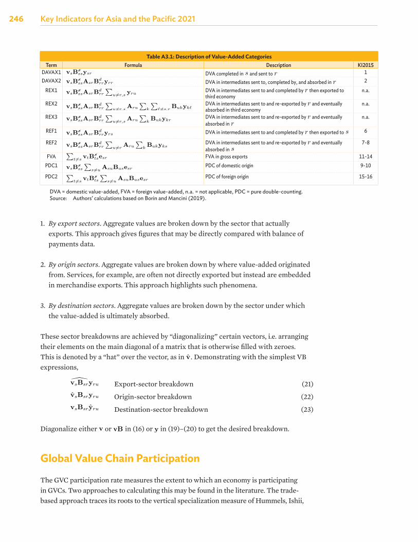
246 Key Indicators for Asia and the Pacific 2021
1. By export sectors. Aggregate values are broken down by the sector that actually exports. This approach gives figures that may be directly compared with balance of payments data.
2. By origin sectors. Aggregate values are broken down by where value-added originated from. Services, for example, are often not directly exported but instead are embedded in merchandise exports. This approach highlights such phenomena.
3. By destination sectors. Aggregate values are broken down by the sector under which the value-added is ultimately absorbed.
These sector breakdowns are achieved by “diagonalizing” certain vectors, i.e. arranging their elements on the main diagonal of a matrix that is otherwise filled with zeroes. This is denoted by a “hat” over the vector, as in
Table A3.1.1: Description of Value-Added Categories
Term Formula Description KI2015
DAVAX1 vsBsssysr DVA completed in s and sent to r 1
DAVAX2 vsBsssAsrBd
rryrr DVA in intermediates sent to, completedby, and absorbed in r
2
REX1 vsBsssAsrBd
rr
∑u=r,s
yru DVA in intermediates sent to andcompleted by r then exported to thirdeconomy
n.a.
REX2 vsBsssAsrBd
rr
∑u=r,s
Aru
∑k
∑ℓ=s,r
Bukykℓ DVA in intermediates sent to andre-exported by r and eventuallyabsorbed in third economy
n.a.
REX3 vsBsssAsrBd
rr
∑u=r,s
Aru
∑k
Bukykr DVA in intermediates sent to andre-exported by r and eventuallyabsorbed in r
n.a.
REF1 vsBsssAsrBd
rryrs DVA in intermediates sent to andcompleted by r then exported to s
6
REF2 vsBsssAsrBd
rr
∑u=r
Aru
∑k
Bukyks DVA in intermediates sent to andre-exported by r and eventuallyabsorbed in s
7–8
FVA∑
t=svtBs
tsesr FVA in gross exports 11–14
PDC1 vsBsss
∑s=u
AsuBusesr PDC of domestic origin 9–10
PDC2∑
t=svtBs
ts
∑s=u
AsuBusesr PDC of foreign origin 15–16
DVA = domestic value-added, FVA = foreign value-added, PDC = pure double-counting
Source: Authors’ calculations based on Borin and Mancini (2019).
1. By export sectors. Aggregate values are broken down by the sector that actually exports. This approachgives figures that may be directly compared with balance of payments data.
2. By origin sectors. Aggregate values are broken down by where value-added originated from. Services,for example, are often not directly exported but instead are embedded in merchandise exports. Thisapproach highlights such phenomena.
3. By destination sectors. Aggregate values are broken down by the sector under which the value-addedis ultimately absorbed.
These sector breakdowns are achieved by “diagonalizing” certain vectors, i.e. arranging their elements on themain diagonal of a matrix that is otherwise filled with zeroes. This is denoted by a “hat” over the vector, asin v. Demonstrating with the simplest VB expressions,
vsBsryru Export-sector breakdown (21)
vsBsryru Origin-sector breakdown (22)
vsBsryru Destination-sector breakdown (23)
Diagonalize either v or vB in (16) or y in (19)–(20) to get the desired breakdown.
9
. Demonstrating with the simplest VB expressions,
Export-sector breakdown (21)
Origin-sector breakdown (22)
Destination-sector breakdown (23)
Diagonalize either
Table A3.1.1: Description of Value-Added Categories
Term Formula Description KI2015
DAVAX1 vsBsssysr DVA completed in s and sent to r 1
DAVAX2 vsBsssAsrBd
rryrr DVA in intermediates sent to, completedby, and absorbed in r
2
REX1 vsBsssAsrBd
rr
∑u=r,s
yru DVA in intermediates sent to andcompleted by r then exported to thirdeconomy
n.a.
REX2 vsBsssAsrBd
rr
∑u=r,s
Aru
∑k
∑ℓ=s,r
Bukykℓ DVA in intermediates sent to andre-exported by r and eventuallyabsorbed in third economy
n.a.
REX3 vsBsssAsrBd
rr
∑u=r,s
Aru
∑k
Bukykr DVA in intermediates sent to andre-exported by r and eventuallyabsorbed in r
n.a.
REF1 vsBsssAsrBd
rryrs DVA in intermediates sent to andcompleted by r then exported to s
6
REF2 vsBsssAsrBd
rr
∑u=r
Aru
∑k
Bukyks DVA in intermediates sent to andre-exported by r and eventuallyabsorbed in s
7–8
FVA∑
t=svtBs
tsesr FVA in gross exports 11–14
PDC1 vsBsss
∑s=u
AsuBusesr PDC of domestic origin 9–10
PDC2∑
t=svtBs
ts
∑s=u
AsuBusesr PDC of foreign origin 15–16
DVA = domestic value-added, FVA = foreign value-added, PDC = pure double-counting
Source: Authors’ calculations based on Borin and Mancini (2019).
1. By export sectors. Aggregate values are broken down by the sector that actually exports. This approachgives figures that may be directly compared with balance of payments data.
2. By origin sectors. Aggregate values are broken down by where value-added originated from. Services,for example, are often not directly exported but instead are embedded in merchandise exports. Thisapproach highlights such phenomena.
3. By destination sectors. Aggregate values are broken down by the sector under which the value-addedis ultimately absorbed.
These sector breakdowns are achieved by “diagonalizing” certain vectors, i.e. arranging their elements on themain diagonal of a matrix that is otherwise filled with zeroes. This is denoted by a “hat” over the vector, asin v. Demonstrating with the simplest VB expressions,
vsBsryru Export-sector breakdown (21)
vsBsryru Origin-sector breakdown (22)
vsBsryru Destination-sector breakdown (23)
Diagonalize either v or vB in (16) or y in (19)–(20) to get the desired breakdown.
9
or
Table A3.1.1: Description of Value-Added Categories
Term Formula Description KI2015
DAVAX1 vsBsssysr DVA completed in s and sent to r 1
DAVAX2 vsBsssAsrBd
rryrr DVA in intermediates sent to, completedby, and absorbed in r
2
REX1 vsBsssAsrBd
rr
∑u=r,s
yru DVA in intermediates sent to andcompleted by r then exported to thirdeconomy
n.a.
REX2 vsBsssAsrBd
rr
∑u=r,s
Aru
∑k
∑ℓ=s,r
Bukykℓ DVA in intermediates sent to andre-exported by r and eventuallyabsorbed in third economy
n.a.
REX3 vsBsssAsrBd
rr
∑u=r,s
Aru
∑k
Bukykr DVA in intermediates sent to andre-exported by r and eventuallyabsorbed in r
n.a.
REF1 vsBsssAsrBd
rryrs DVA in intermediates sent to andcompleted by r then exported to s
6
REF2 vsBsssAsrBd
rr
∑u=r
Aru
∑k
Bukyks DVA in intermediates sent to andre-exported by r and eventuallyabsorbed in s
7–8
FVA∑
t=svtBs
tsesr FVA in gross exports 11–14
PDC1 vsBsss
∑s=u
AsuBusesr PDC of domestic origin 9–10
PDC2∑
t=svtBs
ts
∑s=u
AsuBusesr PDC of foreign origin 15–16
DVA = domestic value-added, FVA = foreign value-added, PDC = pure double-counting
Source: Authors’ calculations based on Borin and Mancini (2019).
1. By export sectors. Aggregate values are broken down by the sector that actually exports. This approachgives figures that may be directly compared with balance of payments data.
2. By origin sectors. Aggregate values are broken down by where value-added originated from. Services,for example, are often not directly exported but instead are embedded in merchandise exports. Thisapproach highlights such phenomena.
3. By destination sectors. Aggregate values are broken down by the sector under which the value-addedis ultimately absorbed.
These sector breakdowns are achieved by “diagonalizing” certain vectors, i.e. arranging their elements on themain diagonal of a matrix that is otherwise filled with zeroes. This is denoted by a “hat” over the vector, asin v. Demonstrating with the simplest VB expressions,
vsBsryru Export-sector breakdown (21)
vsBsryru Origin-sector breakdown (22)
vsBsryru Destination-sector breakdown (23)
Diagonalize either v or vB in (16) or y in (19)–(20) to get the desired breakdown.
9
in (16) or
Table A3.1.1: Description of Value-Added Categories
Term Formula Description KI2015
DAVAX1 vsBsssysr DVA completed in s and sent to r 1
DAVAX2 vsBsssAsrBd
rryrr DVA in intermediates sent to, completedby, and absorbed in r
2
REX1 vsBsssAsrBd
rr
∑u=r,s
yru DVA in intermediates sent to andcompleted by r then exported to thirdeconomy
n.a.
REX2 vsBsssAsrBd
rr
∑u=r,s
Aru
∑k
∑ℓ=s,r
Bukykℓ DVA in intermediates sent to andre-exported by r and eventuallyabsorbed in third economy
n.a.
REX3 vsBsssAsrBd
rr
∑u=r,s
Aru
∑k
Bukykr DVA in intermediates sent to andre-exported by r and eventuallyabsorbed in r
n.a.
REF1 vsBsssAsrBd
rryrs DVA in intermediates sent to andcompleted by r then exported to s
6
REF2 vsBsssAsrBd
rr
∑u=r
Aru
∑k
Bukyks DVA in intermediates sent to andre-exported by r and eventuallyabsorbed in s
7–8
FVA∑
t=svtBs
tsesr FVA in gross exports 11–14
PDC1 vsBsss
∑s=u
AsuBusesr PDC of domestic origin 9–10
PDC2∑
t=svtBs
ts
∑s=u
AsuBusesr PDC of foreign origin 15–16
DVA = domestic value-added, FVA = foreign value-added, PDC = pure double-counting
Source: Authors’ calculations based on Borin and Mancini (2019).
1. By export sectors. Aggregate values are broken down by the sector that actually exports. This approachgives figures that may be directly compared with balance of payments data.
2. By origin sectors. Aggregate values are broken down by where value-added originated from. Services,for example, are often not directly exported but instead are embedded in merchandise exports. Thisapproach highlights such phenomena.
3. By destination sectors. Aggregate values are broken down by the sector under which the value-addedis ultimately absorbed.
These sector breakdowns are achieved by “diagonalizing” certain vectors, i.e. arranging their elements on themain diagonal of a matrix that is otherwise filled with zeroes. This is denoted by a “hat” over the vector, asin v. Demonstrating with the simplest VB expressions,
vsBsryru Export-sector breakdown (21)
vsBsryru Origin-sector breakdown (22)
vsBsryru Destination-sector breakdown (23)
Diagonalize either v or vB in (16) or y in (19)–(20) to get the desired breakdown.
9
in (19)–(20) to get the desired breakdown.
Global Value Chain Participation
The GVC participation rate measures the extent to which an economy is participating in GVCs. Two approaches to calculating this may be found in the literature. The trade-based approach traces its roots to the vertical specialization measure of Hummels, Ishii,
Table A3.1: Description of Value-Added CategoriesTerm Formula Description KI2015
DAVAX1 DVA completed in
element v(s,i) ≡ va(s,i)/x(s,i). This gives the value-added-to-output ratio for each economy–sector. It followsthat
∑(s,j) a(s,j),(r,i) + v(r,i) = 1. Premultiplying this to (11) converts everything to value-added terms:
vsxs ≡ vas = vs
G∑r
G∑u
Bsryru. (12)
Note that this ends up summing sector-level quantities into the aggregate level. To prevent this, see thesection on sector breakdowns.
This expression gives the value-added generated in economy s that is eventually consumed in economy u.It can be tweaked to measure other flows. For example, vsBsryru considers s value-added embodied infinal goods completed in r that are sold to u. To measure s value-added embodied in r’s total exports, onemay instead write vsBsrer∗. These expressions are called VB decompositions and they serve to identify thevalue-added origins of certain quantities.
Even more specific flows may be derived by defining input use structures for domestic intermediates Zd andforeign intermediates Zf separately, yielding Ad and Af where A = Ad +Af . Equation (8) can be rewrittenas
x = (Adx + yd) + (Af x + yf ). (13)
Moreover, since Zf i = Af x, the exports vector (6) can also be rewritten as
e = Af x + yf . (14)
Plugging this into (13) and solving for x,
x = (Adx + yd) + e
= (I − Ad)−1(yd + e)
= Bd(yd + e). (15)
The matrix Bd is called the local Leontief inverse matrix. Its interpretation is the same as the B matrix,except it assumes an input structure that precludes buying and selling inputs abroad. As such, only theblock diagonal elements are non-zero. This isolates the purely domestic portion of production. ComparevsBssyss and vsBd
ssyss. While they both meaure s value-added in its own final consumption, the firstexpression allows for some processing abroad while the second restricts it to purely domestic linkages. Thiswill be crucial in disentangling direct and indirect trading.
Decomposing Exports into Value-Added Categories
Gross exports mask several distinct forms of trading. A substantial portion for most economies is directtrading, where value-added crosses one border before being consumed. The rest involves indirect trading,which itself can take three forms. It can arise from the use of imported inputs, so that one economy’s exportscontain value-added from another economy. It can arise from re-exports, so that one economy’s value-addedgets absorbed somewhere other than its direct importer. Finally, it can arise from what is called “pure”
5
and sent to
where ⊗ denote a Kronecker product. Written out,
E ≡
0 zC1,J1 + zC1,J2 zC1,U1 + zC1,U2
0 zC2,J1 + zC2,J2 zC2,U1 + zC2,U2
zJ1,C1 + zJ1,C2 0 zJ1,U1 + zJ1,U2
zJ2,C1 + zJ2,C2 0 zJ2,U1 + zJ2,U2
zU1,C1 + zU1,C2 zU1,J1 + zU1,J2 0zU2,C1 + zU2,C2 zU2,J1 + zU2,J2 0
+
0 yC1,J yC1,U
0 yC2,J yC2,U
yJ1,C 0 yJ1,U
yJ2,C 0 yJ2,U
yU1,C yU1,J 0yU2,C yU2,J 0
=
0 eC1,J eC1,U
0 eC2,J eC2,U
eJ1,C 0 eJ1,U
eJ2,C 0 eJ2,U
eU1,C eU1,J 0eU2,C eU2,J 0
=
0 eCJ eCU
eJC 0 eJU
eUC eUJ 0
The technical coefficient a(s,j),(r,i) is the share of inputs from (s, j) in the output of (r, i): a(s,j),(r,i) ≡z(s,j),(r,i)/x(r,i). Collect all these into the GN × GN matrix of technical coefficients A. This may be used torewrite (3) as
x = Ax + y. (8)
Solving for x gives
x = (I − A)−1y = By, (9)
where the GN × GN matrix B is called the global Leontief inverse matrix.
VB Decomposition
Equation (9) is central to analyzing cross-economy and cross-sectoral linkages. It is clearer to see this if (8)and (9) are rewritten to isolate a single economy s:
xs =Gr
Asrxr +Gr
ysr (10)
=Gr
Gu
Bsryru (11)
Equation (10) says that s’s output xs is used as intermediates in r’s output or sold as final goods to r (for allr = 1, ..., G). The output of each r can in turn be used as intermediates by other economies, whose outputsare then used by further economies, and so on in a potentially infinite series of production stages. Equation(11) summarizes these to identify the final landing stage of s’s output. The product Bsryru is s output thatis “completed” into a final good by r, which then sends it to u for final absorption.
In most analyses, value-added rather than output is the preferred metric. Define the vector v with (s, i)th
4
1DAVAX2 DVA in intermediates sent to, completed by, and absorbed in
where ⊗ denote a Kronecker product. Written out,
E ≡
0 zC1,J1 + zC1,J2 zC1,U1 + zC1,U2
0 zC2,J1 + zC2,J2 zC2,U1 + zC2,U2
zJ1,C1 + zJ1,C2 0 zJ1,U1 + zJ1,U2
zJ2,C1 + zJ2,C2 0 zJ2,U1 + zJ2,U2
zU1,C1 + zU1,C2 zU1,J1 + zU1,J2 0zU2,C1 + zU2,C2 zU2,J1 + zU2,J2 0
+
0 yC1,J yC1,U
0 yC2,J yC2,U
yJ1,C 0 yJ1,U
yJ2,C 0 yJ2,U
yU1,C yU1,J 0yU2,C yU2,J 0
=
0 eC1,J eC1,U
0 eC2,J eC2,U
eJ1,C 0 eJ1,U
eJ2,C 0 eJ2,U
eU1,C eU1,J 0eU2,C eU2,J 0
=
0 eCJ eCU
eJC 0 eJU
eUC eUJ 0
The technical coefficient a(s,j),(r,i) is the share of inputs from (s, j) in the output of (r, i): a(s,j),(r,i) ≡z(s,j),(r,i)/x(r,i). Collect all these into the GN × GN matrix of technical coefficients A. This may be used torewrite (3) as
x = Ax + y. (8)
Solving for x gives
x = (I − A)−1y = By, (9)
where the GN × GN matrix B is called the global Leontief inverse matrix.
VB Decomposition
Equation (9) is central to analyzing cross-economy and cross-sectoral linkages. It is clearer to see this if (8)and (9) are rewritten to isolate a single economy s:
xs =Gr
Asrxr +Gr
ysr (10)
=Gr
Gu
Bsryru (11)
Equation (10) says that s’s output xs is used as intermediates in r’s output or sold as final goods to r (for allr = 1, ..., G). The output of each r can in turn be used as intermediates by other economies, whose outputsare then used by further economies, and so on in a potentially infinite series of production stages. Equation(11) summarizes these to identify the final landing stage of s’s output. The product Bsryru is s output thatis “completed” into a final good by r, which then sends it to u for final absorption.
In most analyses, value-added rather than output is the preferred metric. Define the vector v with (s, i)th
4
2
REX1 DVA in intermediates sent to and completed by
where ⊗ denote a Kronecker product. Written out,
E ≡
0 zC1,J1 + zC1,J2 zC1,U1 + zC1,U2
0 zC2,J1 + zC2,J2 zC2,U1 + zC2,U2
zJ1,C1 + zJ1,C2 0 zJ1,U1 + zJ1,U2
zJ2,C1 + zJ2,C2 0 zJ2,U1 + zJ2,U2
zU1,C1 + zU1,C2 zU1,J1 + zU1,J2 0zU2,C1 + zU2,C2 zU2,J1 + zU2,J2 0
+
0 yC1,J yC1,U
0 yC2,J yC2,U
yJ1,C 0 yJ1,U
yJ2,C 0 yJ2,U
yU1,C yU1,J 0yU2,C yU2,J 0
=
0 eC1,J eC1,U
0 eC2,J eC2,U
eJ1,C 0 eJ1,U
eJ2,C 0 eJ2,U
eU1,C eU1,J 0eU2,C eU2,J 0
=
0 eCJ eCU
eJC 0 eJU
eUC eUJ 0
The technical coefficient a(s,j),(r,i) is the share of inputs from (s, j) in the output of (r, i): a(s,j),(r,i) ≡z(s,j),(r,i)/x(r,i). Collect all these into the GN × GN matrix of technical coefficients A. This may be used torewrite (3) as
x = Ax + y. (8)
Solving for x gives
x = (I − A)−1y = By, (9)
where the GN × GN matrix B is called the global Leontief inverse matrix.
VB Decomposition
Equation (9) is central to analyzing cross-economy and cross-sectoral linkages. It is clearer to see this if (8)and (9) are rewritten to isolate a single economy s:
xs =Gr
Asrxr +Gr
ysr (10)
=Gr
Gu
Bsryru (11)
Equation (10) says that s’s output xs is used as intermediates in r’s output or sold as final goods to r (for allr = 1, ..., G). The output of each r can in turn be used as intermediates by other economies, whose outputsare then used by further economies, and so on in a potentially infinite series of production stages. Equation(11) summarizes these to identify the final landing stage of s’s output. The product Bsryru is s output thatis “completed” into a final good by r, which then sends it to u for final absorption.
In most analyses, value-added rather than output is the preferred metric. Define the vector v with (s, i)th
4
then exported to third economy
n.a.
REX2 DVA in intermediates sent to and re-exported by
where ⊗ denote a Kronecker product. Written out,
E ≡
0 zC1,J1 + zC1,J2 zC1,U1 + zC1,U2
0 zC2,J1 + zC2,J2 zC2,U1 + zC2,U2
zJ1,C1 + zJ1,C2 0 zJ1,U1 + zJ1,U2
zJ2,C1 + zJ2,C2 0 zJ2,U1 + zJ2,U2
zU1,C1 + zU1,C2 zU1,J1 + zU1,J2 0zU2,C1 + zU2,C2 zU2,J1 + zU2,J2 0
+
0 yC1,J yC1,U
0 yC2,J yC2,U
yJ1,C 0 yJ1,U
yJ2,C 0 yJ2,U
yU1,C yU1,J 0yU2,C yU2,J 0
=
0 eC1,J eC1,U
0 eC2,J eC2,U
eJ1,C 0 eJ1,U
eJ2,C 0 eJ2,U
eU1,C eU1,J 0eU2,C eU2,J 0
=
0 eCJ eCU
eJC 0 eJU
eUC eUJ 0
The technical coefficient a(s,j),(r,i) is the share of inputs from (s, j) in the output of (r, i): a(s,j),(r,i) ≡z(s,j),(r,i)/x(r,i). Collect all these into the GN × GN matrix of technical coefficients A. This may be used torewrite (3) as
x = Ax + y. (8)
Solving for x gives
x = (I − A)−1y = By, (9)
where the GN × GN matrix B is called the global Leontief inverse matrix.
VB Decomposition
Equation (9) is central to analyzing cross-economy and cross-sectoral linkages. It is clearer to see this if (8)and (9) are rewritten to isolate a single economy s:
xs =Gr
Asrxr +Gr
ysr (10)
=Gr
Gu
Bsryru (11)
Equation (10) says that s’s output xs is used as intermediates in r’s output or sold as final goods to r (for allr = 1, ..., G). The output of each r can in turn be used as intermediates by other economies, whose outputsare then used by further economies, and so on in a potentially infinite series of production stages. Equation(11) summarizes these to identify the final landing stage of s’s output. The product Bsryru is s output thatis “completed” into a final good by r, which then sends it to u for final absorption.
In most analyses, value-added rather than output is the preferred metric. Define the vector v with (s, i)th
4
and eventually absorbed in third economy
n.a.
REX3 DVA in intermediates sent to and re-exported by
where ⊗ denote a Kronecker product. Written out,
E ≡
0 zC1,J1 + zC1,J2 zC1,U1 + zC1,U2
0 zC2,J1 + zC2,J2 zC2,U1 + zC2,U2
zJ1,C1 + zJ1,C2 0 zJ1,U1 + zJ1,U2
zJ2,C1 + zJ2,C2 0 zJ2,U1 + zJ2,U2
zU1,C1 + zU1,C2 zU1,J1 + zU1,J2 0zU2,C1 + zU2,C2 zU2,J1 + zU2,J2 0
+
0 yC1,J yC1,U
0 yC2,J yC2,U
yJ1,C 0 yJ1,U
yJ2,C 0 yJ2,U
yU1,C yU1,J 0yU2,C yU2,J 0
=
0 eC1,J eC1,U
0 eC2,J eC2,U
eJ1,C 0 eJ1,U
eJ2,C 0 eJ2,U
eU1,C eU1,J 0eU2,C eU2,J 0
=
0 eCJ eCU
eJC 0 eJU
eUC eUJ 0
The technical coefficient a(s,j),(r,i) is the share of inputs from (s, j) in the output of (r, i): a(s,j),(r,i) ≡z(s,j),(r,i)/x(r,i). Collect all these into the GN × GN matrix of technical coefficients A. This may be used torewrite (3) as
x = Ax + y. (8)
Solving for x gives
x = (I − A)−1y = By, (9)
where the GN × GN matrix B is called the global Leontief inverse matrix.
VB Decomposition
Equation (9) is central to analyzing cross-economy and cross-sectoral linkages. It is clearer to see this if (8)and (9) are rewritten to isolate a single economy s:
xs =Gr
Asrxr +Gr
ysr (10)
=Gr
Gu
Bsryru (11)
Equation (10) says that s’s output xs is used as intermediates in r’s output or sold as final goods to r (for allr = 1, ..., G). The output of each r can in turn be used as intermediates by other economies, whose outputsare then used by further economies, and so on in a potentially infinite series of production stages. Equation(11) summarizes these to identify the final landing stage of s’s output. The product Bsryru is s output thatis “completed” into a final good by r, which then sends it to u for final absorption.
In most analyses, value-added rather than output is the preferred metric. Define the vector v with (s, i)th
4
and eventually absorbed in
where ⊗ denote a Kronecker product. Written out,
E ≡
0 zC1,J1 + zC1,J2 zC1,U1 + zC1,U2
0 zC2,J1 + zC2,J2 zC2,U1 + zC2,U2
zJ1,C1 + zJ1,C2 0 zJ1,U1 + zJ1,U2
zJ2,C1 + zJ2,C2 0 zJ2,U1 + zJ2,U2
zU1,C1 + zU1,C2 zU1,J1 + zU1,J2 0zU2,C1 + zU2,C2 zU2,J1 + zU2,J2 0
+
0 yC1,J yC1,U
0 yC2,J yC2,U
yJ1,C 0 yJ1,U
yJ2,C 0 yJ2,U
yU1,C yU1,J 0yU2,C yU2,J 0
=
0 eC1,J eC1,U
0 eC2,J eC2,U
eJ1,C 0 eJ1,U
eJ2,C 0 eJ2,U
eU1,C eU1,J 0eU2,C eU2,J 0
=
0 eCJ eCU
eJC 0 eJU
eUC eUJ 0
The technical coefficient a(s,j),(r,i) is the share of inputs from (s, j) in the output of (r, i): a(s,j),(r,i) ≡z(s,j),(r,i)/x(r,i). Collect all these into the GN × GN matrix of technical coefficients A. This may be used torewrite (3) as
x = Ax + y. (8)
Solving for x gives
x = (I − A)−1y = By, (9)
where the GN × GN matrix B is called the global Leontief inverse matrix.
VB Decomposition
Equation (9) is central to analyzing cross-economy and cross-sectoral linkages. It is clearer to see this if (8)and (9) are rewritten to isolate a single economy s:
xs =Gr
Asrxr +Gr
ysr (10)
=Gr
Gu
Bsryru (11)
Equation (10) says that s’s output xs is used as intermediates in r’s output or sold as final goods to r (for allr = 1, ..., G). The output of each r can in turn be used as intermediates by other economies, whose outputsare then used by further economies, and so on in a potentially infinite series of production stages. Equation(11) summarizes these to identify the final landing stage of s’s output. The product Bsryru is s output thatis “completed” into a final good by r, which then sends it to u for final absorption.
In most analyses, value-added rather than output is the preferred metric. Define the vector v with (s, i)th
4
n.a.
REF1 DVA in intermediates sent to and completed by
where ⊗ denote a Kronecker product. Written out,
E ≡
0 zC1,J1 + zC1,J2 zC1,U1 + zC1,U2
0 zC2,J1 + zC2,J2 zC2,U1 + zC2,U2
zJ1,C1 + zJ1,C2 0 zJ1,U1 + zJ1,U2
zJ2,C1 + zJ2,C2 0 zJ2,U1 + zJ2,U2
zU1,C1 + zU1,C2 zU1,J1 + zU1,J2 0zU2,C1 + zU2,C2 zU2,J1 + zU2,J2 0
+
0 yC1,J yC1,U
0 yC2,J yC2,U
yJ1,C 0 yJ1,U
yJ2,C 0 yJ2,U
yU1,C yU1,J 0yU2,C yU2,J 0
=
0 eC1,J eC1,U
0 eC2,J eC2,U
eJ1,C 0 eJ1,U
eJ2,C 0 eJ2,U
eU1,C eU1,J 0eU2,C eU2,J 0
=
0 eCJ eCU
eJC 0 eJU
eUC eUJ 0
The technical coefficient a(s,j),(r,i) is the share of inputs from (s, j) in the output of (r, i): a(s,j),(r,i) ≡z(s,j),(r,i)/x(r,i). Collect all these into the GN × GN matrix of technical coefficients A. This may be used torewrite (3) as
x = Ax + y. (8)
Solving for x gives
x = (I − A)−1y = By, (9)
where the GN × GN matrix B is called the global Leontief inverse matrix.
VB Decomposition
Equation (9) is central to analyzing cross-economy and cross-sectoral linkages. It is clearer to see this if (8)and (9) are rewritten to isolate a single economy s:
xs =Gr
Asrxr +Gr
ysr (10)
=Gr
Gu
Bsryru (11)
Equation (10) says that s’s output xs is used as intermediates in r’s output or sold as final goods to r (for allr = 1, ..., G). The output of each r can in turn be used as intermediates by other economies, whose outputsare then used by further economies, and so on in a potentially infinite series of production stages. Equation(11) summarizes these to identify the final landing stage of s’s output. The product Bsryru is s output thatis “completed” into a final good by r, which then sends it to u for final absorption.
In most analyses, value-added rather than output is the preferred metric. Define the vector v with (s, i)th
4
then exported to
element v(s,i) ≡ va(s,i)/x(s,i). This gives the value-added-to-output ratio for each economy–sector. It followsthat
∑(s,j) a(s,j),(r,i) + v(r,i) = 1. Premultiplying this to (11) converts everything to value-added terms:
vsxs ≡ vas = vs
G∑r
G∑u
Bsryru. (12)
Note that this ends up summing sector-level quantities into the aggregate level. To prevent this, see thesection on sector breakdowns.
This expression gives the value-added generated in economy s that is eventually consumed in economy u.It can be tweaked to measure other flows. For example, vsBsryru considers s value-added embodied infinal goods completed in r that are sold to u. To measure s value-added embodied in r’s total exports, onemay instead write vsBsrer∗. These expressions are called VB decompositions and they serve to identify thevalue-added origins of certain quantities.
Even more specific flows may be derived by defining input use structures for domestic intermediates Zd andforeign intermediates Zf separately, yielding Ad and Af where A = Ad +Af . Equation (8) can be rewrittenas
x = (Adx + yd) + (Af x + yf ). (13)
Moreover, since Zf i = Af x, the exports vector (6) can also be rewritten as
e = Af x + yf . (14)
Plugging this into (13) and solving for x,
x = (Adx + yd) + e
= (I − Ad)−1(yd + e)
= Bd(yd + e). (15)
The matrix Bd is called the local Leontief inverse matrix. Its interpretation is the same as the B matrix,except it assumes an input structure that precludes buying and selling inputs abroad. As such, only theblock diagonal elements are non-zero. This isolates the purely domestic portion of production. ComparevsBssyss and vsBd
ssyss. While they both meaure s value-added in its own final consumption, the firstexpression allows for some processing abroad while the second restricts it to purely domestic linkages. Thiswill be crucial in disentangling direct and indirect trading.
Decomposing Exports into Value-Added Categories
Gross exports mask several distinct forms of trading. A substantial portion for most economies is directtrading, where value-added crosses one border before being consumed. The rest involves indirect trading,which itself can take three forms. It can arise from the use of imported inputs, so that one economy’s exportscontain value-added from another economy. It can arise from re-exports, so that one economy’s value-addedgets absorbed somewhere other than its direct importer. Finally, it can arise from what is called “pure”
5
6
REF2 DVA in intermediates sent to and re-exported by
where ⊗ denote a Kronecker product. Written out,
E ≡
0 zC1,J1 + zC1,J2 zC1,U1 + zC1,U2
0 zC2,J1 + zC2,J2 zC2,U1 + zC2,U2
zJ1,C1 + zJ1,C2 0 zJ1,U1 + zJ1,U2
zJ2,C1 + zJ2,C2 0 zJ2,U1 + zJ2,U2
zU1,C1 + zU1,C2 zU1,J1 + zU1,J2 0zU2,C1 + zU2,C2 zU2,J1 + zU2,J2 0
+
0 yC1,J yC1,U
0 yC2,J yC2,U
yJ1,C 0 yJ1,U
yJ2,C 0 yJ2,U
yU1,C yU1,J 0yU2,C yU2,J 0
=
0 eC1,J eC1,U
0 eC2,J eC2,U
eJ1,C 0 eJ1,U
eJ2,C 0 eJ2,U
eU1,C eU1,J 0eU2,C eU2,J 0
=
0 eCJ eCU
eJC 0 eJU
eUC eUJ 0
The technical coefficient a(s,j),(r,i) is the share of inputs from (s, j) in the output of (r, i): a(s,j),(r,i) ≡z(s,j),(r,i)/x(r,i). Collect all these into the GN × GN matrix of technical coefficients A. This may be used torewrite (3) as
x = Ax + y. (8)
Solving for x gives
x = (I − A)−1y = By, (9)
where the GN × GN matrix B is called the global Leontief inverse matrix.
VB Decomposition
Equation (9) is central to analyzing cross-economy and cross-sectoral linkages. It is clearer to see this if (8)and (9) are rewritten to isolate a single economy s:
xs =Gr
Asrxr +Gr
ysr (10)
=Gr
Gu
Bsryru (11)
Equation (10) says that s’s output xs is used as intermediates in r’s output or sold as final goods to r (for allr = 1, ..., G). The output of each r can in turn be used as intermediates by other economies, whose outputsare then used by further economies, and so on in a potentially infinite series of production stages. Equation(11) summarizes these to identify the final landing stage of s’s output. The product Bsryru is s output thatis “completed” into a final good by r, which then sends it to u for final absorption.
In most analyses, value-added rather than output is the preferred metric. Define the vector v with (s, i)th
4
and eventually absorbed in
element v(s,i) ≡ va(s,i)/x(s,i). This gives the value-added-to-output ratio for each economy–sector. It followsthat
∑(s,j) a(s,j),(r,i) + v(r,i) = 1. Premultiplying this to (11) converts everything to value-added terms:
vsxs ≡ vas = vs
G∑r
G∑u
Bsryru. (12)
Note that this ends up summing sector-level quantities into the aggregate level. To prevent this, see thesection on sector breakdowns.
This expression gives the value-added generated in economy s that is eventually consumed in economy u.It can be tweaked to measure other flows. For example, vsBsryru considers s value-added embodied infinal goods completed in r that are sold to u. To measure s value-added embodied in r’s total exports, onemay instead write vsBsrer∗. These expressions are called VB decompositions and they serve to identify thevalue-added origins of certain quantities.
Even more specific flows may be derived by defining input use structures for domestic intermediates Zd andforeign intermediates Zf separately, yielding Ad and Af where A = Ad +Af . Equation (8) can be rewrittenas
x = (Adx + yd) + (Af x + yf ). (13)
Moreover, since Zf i = Af x, the exports vector (6) can also be rewritten as
e = Af x + yf . (14)
Plugging this into (13) and solving for x,
x = (Adx + yd) + e
= (I − Ad)−1(yd + e)
= Bd(yd + e). (15)
The matrix Bd is called the local Leontief inverse matrix. Its interpretation is the same as the B matrix,except it assumes an input structure that precludes buying and selling inputs abroad. As such, only theblock diagonal elements are non-zero. This isolates the purely domestic portion of production. ComparevsBssyss and vsBd
ssyss. While they both meaure s value-added in its own final consumption, the firstexpression allows for some processing abroad while the second restricts it to purely domestic linkages. Thiswill be crucial in disentangling direct and indirect trading.
Decomposing Exports into Value-Added Categories
Gross exports mask several distinct forms of trading. A substantial portion for most economies is directtrading, where value-added crosses one border before being consumed. The rest involves indirect trading,which itself can take three forms. It can arise from the use of imported inputs, so that one economy’s exportscontain value-added from another economy. It can arise from re-exports, so that one economy’s value-addedgets absorbed somewhere other than its direct importer. Finally, it can arise from what is called “pure”
5
7-8
FVA FVA in gross exports 11-14PDC1 PDC of domestic origin 9-10
PDC2 PDC of foreign origin 15-16
DVA = domestic value-added, FVA = foreign value-added, n.a. = not applicable, PDC = pure double-counting. Source: Authors’ calculations based on Borin and Mancini (2019).
Table A3.1.1: Description of Value-Added Categories
Term Formula Description KI2015
DAVAX1 vsBsssysr DVA completed in s and sent to r 1
DAVAX2 vsBsssAsrBd
rryrr DVA in intermediates sent to, completedby, and absorbed in r
2
REX1 vsBsssAsrBd
rr
∑u=r,s
yru DVA in intermediates sent to andcompleted by r then exported to thirdeconomy
n.a.
REX2 vsBsssAsrBd
rr
∑u=r,s
Aru
∑k
∑ℓ=s,r
Bukykℓ DVA in intermediates sent to andre-exported by r and eventuallyabsorbed in third economy
n.a.
REX3 vsBsssAsrBd
rr
∑u=r,s
Aru
∑k
Bukykr DVA in intermediates sent to andre-exported by r and eventuallyabsorbed in r
n.a.
REF1 vsBsssAsrBd
rryrs DVA in intermediates sent to andcompleted by r then exported to s
6
REF2 vsBsssAsrBd
rr
∑u=r
Aru
∑k
Bukyks DVA in intermediates sent to andre-exported by r and eventuallyabsorbed in s
7–8
FVA∑
t=svtBs
tsesr FVA in gross exports 11–14
PDC1 vsBsss
∑s=u
AsuBusesr PDC of domestic origin 9–10
PDC2∑
t=svtBs
ts
∑s=u
AsuBusesr PDC of foreign origin 15–16
DVA = domestic value-added, FVA = foreign value-added, PDC = pure double-counting
Source: Authors’ calculations based on Borin and Mancini (2019).
1. By export sectors. Aggregate values are broken down by the sector that actually exports. This approachgives figures that may be directly compared with balance of payments data.
2. By origin sectors. Aggregate values are broken down by where value-added originated from. Services,for example, are often not directly exported but instead are embedded in merchandise exports. Thisapproach highlights such phenomena.
3. By destination sectors. Aggregate values are broken down by the sector under which the value-addedis ultimately absorbed.
These sector breakdowns are achieved by “diagonalizing” certain vectors, i.e. arranging their elements on themain diagonal of a matrix that is otherwise filled with zeroes. This is denoted by a “hat” over the vector, asin v. Demonstrating with the simplest VB expressions,
vsBsryru Export-sector breakdown (21)
vsBsryru Origin-sector breakdown (22)
vsBsryru Destination-sector breakdown (23)
Diagonalize either v or vB in (16) or y in (19)–(20) to get the desired breakdown.
9
Table A3.1.1: Description of Value-Added Categories
Term Formula Description KI2015
DAVAX1 vsBsssysr DVA completed in s and sent to r 1
DAVAX2 vsBsssAsrBd
rryrr DVA in intermediates sent to, completedby, and absorbed in r
2
REX1 vsBsssAsrBd
rr
∑u=r,s
yru DVA in intermediates sent to andcompleted by r then exported to thirdeconomy
n.a.
REX2 vsBsssAsrBd
rr
∑u=r,s
Aru
∑k
∑ℓ=s,r
Bukykℓ DVA in intermediates sent to andre-exported by r and eventuallyabsorbed in third economy
n.a.
REX3 vsBsssAsrBd
rr
∑u =r,s
Aru
∑k
Bukykr DVA in intermediates sent to andre-exported by r and eventuallyabsorbed in r
n.a.
REF1 vsBsssAsrBd
rryrs DVA in intermediates sent to andcompleted by r then exported to s
6
REF2 vsBsssAsrBd
rr
∑u=r
Aru
∑k
Bukyks DVA in intermediates sent to andre-exported by r and eventuallyabsorbed in s
7–8
FVA∑
t=svtBs
tsesr FVA in gross exports 11–14
PDC1 vsBsss
∑s=u
AsuBusesr PDC of domestic origin 9–10
PDC2∑
t=svtBs
ts
∑s=u
AsuBusesr PDC of foreign origin 15–16
DVA = domestic value-added, FVA = foreign value-added, PDC = pure double-counting
Source: Authors’ calculations based on Borin and Mancini (2019).
1. By export sectors. Aggregate values are broken down by the sector that actually exports. This approachgives figures that may be directly compared with balance of payments data.
2. By origin sectors. Aggregate values are broken down by where value-added originated from. Services,for example, are often not directly exported but instead are embedded in merchandise exports. Thisapproach highlights such phenomena.
3. By destination sectors. Aggregate values are broken down by the sector under which the value-addedis ultimately absorbed.
These sector breakdowns are achieved by “diagonalizing” certain vectors, i.e. arranging their elements on themain diagonal of a matrix that is otherwise filled with zeroes. This is denoted by a “hat” over the vector, asin v. Demonstrating with the simplest VB expressions,
vsBsryru Export-sector breakdown (21)
vsBsryru Origin-sector breakdown (22)
vsBsryru Destination-sector breakdown (23)
Diagonalize either v or vB in (16) or y in (19)–(20) to get the desired breakdown.
9
Table A3.1.1: Description of Value-Added Categories
Term Formula Description KI2015
DAVAX1 vsBsssysr DVA completed in s and sent to r 1
DAVAX2 vsBsssAsrBd
rryrr DVA in intermediates sent to, completedby, and absorbed in r
2
REX1 vsBsssAsrBd
rr
∑u=r,s
yru DVA in intermediates sent to andcompleted by r then exported to thirdeconomy
n.a.
REX2 vsBsssAsrBd
rr
∑u=r,s
Aru
∑k
∑ℓ=s,r
Bukykℓ DVA in intermediates sent to andre-exported by r and eventuallyabsorbed in third economy
n.a.
REX3 vsBsssAsrBd
rr
∑u=r,s
Aru
∑k
Bukykr DVA in intermediates sent to andre-exported by r and eventuallyabsorbed in r
n.a.
REF1 vsBsssAsrBd
rryrs DVA in intermediates sent to andcompleted by r then exported to s
6
REF2 vsBsssAsrBd
rr
∑u=r
Aru
∑k
Bukyks DVA in intermediates sent to andre-exported by r and eventuallyabsorbed in s
7–8
FVA∑
t=svtBs
tsesr FVA in gross exports 11–14
PDC1 vsBsss
∑s =u
AsuBusesr PDC of domestic origin 9–10
PDC2∑
t=svtBs
ts
∑s=u
AsuBusesr PDC of foreign origin 15–16
DVA = domestic value-added, FVA = foreign value-added, PDC = pure double-counting
Source: Authors’ calculations based on Borin and Mancini (2019).
1. By export sectors. Aggregate values are broken down by the sector that actually exports. This approachgives figures that may be directly compared with balance of payments data.
2. By origin sectors. Aggregate values are broken down by where value-added originated from. Services,for example, are often not directly exported but instead are embedded in merchandise exports. Thisapproach highlights such phenomena.
3. By destination sectors. Aggregate values are broken down by the sector under which the value-addedis ultimately absorbed.
These sector breakdowns are achieved by “diagonalizing” certain vectors, i.e. arranging their elements on themain diagonal of a matrix that is otherwise filled with zeroes. This is denoted by a “hat” over the vector, asin v. Demonstrating with the simplest VB expressions,
vsBsryru Export-sector breakdown (21)
vsBsryru Origin-sector breakdown (22)
vsBsryru Destination-sector breakdown (23)
Diagonalize either v or vB in (16) or y in (19)–(20) to get the desired breakdown.
9
Table A3.1.1: Description of Value-Added Categories
Term Formula Description KI2015
DAVAX1 vsBsssysr DVA completed in s and sent to r 1
DAVAX2 vsBsssAsrBd
rryrr DVA in intermediates sent to, completedby, and absorbed in r
2
REX1 vsBsssAsrBd
rr
∑u=r,s
yru DVA in intermediates sent to andcompleted by r then exported to thirdeconomy
n.a.
REX2 vsBsssAsrBd
rr
∑u=r,s
Aru
∑k
∑ℓ=s,r
Bukykℓ DVA in intermediates sent to andre-exported by r and eventuallyabsorbed in third economy
n.a.
REX3 vsBsssAsrBd
rr
∑u=r,s
Aru
∑k
Bukykr DVA in intermediates sent to andre-exported by r and eventuallyabsorbed in r
n.a.
REF1 vsBsssAsrBd
rryrs DVA in intermediates sent to andcompleted by r then exported to s
6
REF2 vsBsssAsrBd
rr
∑u=r
Aru
∑k
Bukyks DVA in intermediates sent to andre-exported by r and eventuallyabsorbed in s
7–8
FVA∑
t=svtBs
tsesr FVA in gross exports 11–14
PDC1 vsBsss
∑s=u
AsuBusesr PDC of domestic origin 9–10
PDC2∑
t=svtBs
ts
∑s=u
AsuBusesr PDC of foreign origin 15–16
DVA = domestic value-added, FVA = foreign value-added, PDC = pure double-counting
Source: Authors’ calculations based on Borin and Mancini (2019).
1. By export sectors. Aggregate values are broken down by the sector that actually exports. This approachgives figures that may be directly compared with balance of payments data.
2. By origin sectors. Aggregate values are broken down by where value-added originated from. Services,for example, are often not directly exported but instead are embedded in merchandise exports. Thisapproach highlights such phenomena.
3. By destination sectors. Aggregate values are broken down by the sector under which the value-addedis ultimately absorbed.
These sector breakdowns are achieved by “diagonalizing” certain vectors, i.e. arranging their elements on themain diagonal of a matrix that is otherwise filled with zeroes. This is denoted by a “hat” over the vector, asin v. Demonstrating with the simplest VB expressions,
vsBsryru Export-sector breakdown (21)
vsBsryru Origin-sector breakdown (22)
vsBsryru Destination-sector breakdown (23)
Diagonalize either v or vB in (16) or y in (19)–(20) to get the desired breakdown.
9
Global Value Chains
247Global Value Chains
and Yi (2001), who defined GVCs as trade that crosses at least two borders before final consumption—what might be called indirect trade. Their paper only provides a backward measure of this in the form of the import content of exports. Calculation of the forward end—exports that are re-exported by the direct partner—would only come with the trade accounting framework of Koopman et al. (2014). In the terminology of Borin and Mancini (2019), vertical specialization becomes GVC exports (GVCX) and are defined as follows:
(24) (25)
Total GVC exports are the sum of the two. The trade-based GVC participation rate is obtained by dividing these with gross exports.
Global Value Chain Participation
The GVC participation rate measures the extent to which an economy is participating in GVCs. Twoapproaches to calculating this may be found in the literature. The trade-based approach traces its rootsto the vertical specialization measure of Hummels, Ishii, and Yi (2001), who defined GVCs as trade thatcrosses at least two borders before final consumption—what might be called indirect trade. Their paperonly provides a backward measure of this in the form of the import content of exports. Calculation of theforward end—exports that are re-exported by the direct partner—would only come with the trade accountingframework of Koopman et al. (2014). In the terminology of Borin and Mancini (2019), vertical specializationbecomes GVC exports (GV CX) and are defined as follows:
GV CXbackwardsr = FV Asr + PDCsr, (24)
GV CXforwardsr = REXsr + REF sr. (25)
Total GVC exports are the sum of the two. The trade-based GVC participation rate is obtained by dividingthese with gross exports.
GV CP Tradesr = GV CXbackwardsr
Esr+ GV CXforwardsr
Esr. (26)
This may be split up to include only backward GVCs or only forward GVCs. It may also be summed acrossall trading partners r to get an overall rate. In breaking this rate down by sector, it is more intuitive to usethe export-sector breakdown since the denominator is gross exports.
Alternatively, Wang, Wei, Yu, and Zhu (2017) propose a production-based measure of GVC participation,computed as follows:7
GV CP Productions =
∑r =s DAV AX2sr + REXsr + REF sr
vas. (27)
This is the share of domestic value-added sent abroad in an unfinished state. Note that this is defined onlyfor the sum of s’s trading partners. In breaking this rate down by sector, it is more intuitive to use theorigin-sector breakdown since the denominator is domestic value-added. # Revealed Comparative Advantage
The revealed comparative advantage (RCA) index is a classic trade indicator first proposed by Béla Balassa(1965). It uses existing patterns of trade to identify where an economy’s comparative advantage lies.Formally, the economy s’s RCA index for sector i is given by
RCA(s,i) =E(s,i)/Es∑
r E(r,i)/∑
r Er, (28)
where∑
r E(r,i) is the sum of sector i exports from all economies and∑
r Er is the total exports of alleconomies. This compares the share of i in s’s exports with the average share of i in all economies’ exports.If RCA(s,i) > 1, then economy s is said to have a revealed comparative advantage in sector i. For example,if textiles are 50% of Cambodia’s exports while for the average economy textiles are only 40% of exports,then Cambodia’s RCA index in textiles is 50/40 = 1.25, which implies that it is specializing in that sector.
7This is called the forward GVC participation rate by Wang et al. (2017). Their backward GVC participation rate is notcovered in this framework.
10
(26)
This may be split up to include only backward GVCs or only forward GVCs. It may also be summed across all trading partners
where ⊗ denote a Kronecker product. Written out,
E ≡
0 zC1,J1 + zC1,J2 zC1,U1 + zC1,U2
0 zC2,J1 + zC2,J2 zC2,U1 + zC2,U2
zJ1,C1 + zJ1,C2 0 zJ1,U1 + zJ1,U2
zJ2,C1 + zJ2,C2 0 zJ2,U1 + zJ2,U2
zU1,C1 + zU1,C2 zU1,J1 + zU1,J2 0zU2,C1 + zU2,C2 zU2,J1 + zU2,J2 0
+
0 yC1,J yC1,U
0 yC2,J yC2,U
yJ1,C 0 yJ1,U
yJ2,C 0 yJ2,U
yU1,C yU1,J 0yU2,C yU2,J 0
=
0 eC1,J eC1,U
0 eC2,J eC2,U
eJ1,C 0 eJ1,U
eJ2,C 0 eJ2,U
eU1,C eU1,J 0eU2,C eU2,J 0
=
0 eCJ eCU
eJC 0 eJU
eUC eUJ 0
The technical coefficient a(s,j),(r,i) is the share of inputs from (s, j) in the output of (r, i): a(s,j),(r,i) ≡z(s,j),(r,i)/x(r,i). Collect all these into the GN × GN matrix of technical coefficients A. This may be used torewrite (3) as
x = Ax + y. (8)
Solving for x gives
x = (I − A)−1y = By, (9)
where the GN × GN matrix B is called the global Leontief inverse matrix.
VB Decomposition
Equation (9) is central to analyzing cross-economy and cross-sectoral linkages. It is clearer to see this if (8)and (9) are rewritten to isolate a single economy s:
xs =Gr
Asrxr +Gr
ysr (10)
=Gr
Gu
Bsryru (11)
Equation (10) says that s’s output xs is used as intermediates in r’s output or sold as final goods to r (for allr = 1, ..., G). The output of each r can in turn be used as intermediates by other economies, whose outputsare then used by further economies, and so on in a potentially infinite series of production stages. Equation(11) summarizes these to identify the final landing stage of s’s output. The product Bsryru is s output thatis “completed” into a final good by r, which then sends it to u for final absorption.
In most analyses, value-added rather than output is the preferred metric. Define the vector v with (s, i)th
4
to get an overall rate. In breaking this rate down by sector, it is more intuitive to use the export-sector breakdown since the denominator is gross exports.
Alternatively, Wang, Wei, Yu, and Zhu (2017) propose a production-based measure of GVC participation, computed as follows:8
Global Value Chain Participation
The GVC participation rate measures the extent to which an economy is participating in GVCs. Twoapproaches to calculating this may be found in the literature. The trade-based approach traces its rootsto the vertical specialization measure of Hummels, Ishii, and Yi (2001), who defined GVCs as trade thatcrosses at least two borders before final consumption—what might be called indirect trade. Their paperonly provides a backward measure of this in the form of the import content of exports. Calculation of theforward end—exports that are re-exported by the direct partner—would only come with the trade accountingframework of Koopman et al. (2014). In the terminology of Borin and Mancini (2019), vertical specializationbecomes GVC exports (GV CX) and are defined as follows:
GV CXbackwardsr = FV Asr + PDCsr, (24)
GV CXforwardsr = REXsr + REF sr. (25)
Total GVC exports are the sum of the two. The trade-based GVC participation rate is obtained by dividingthese with gross exports.
GV CP Tradesr = GV CXbackwardsr
Esr+ GV CXforwardsr
Esr. (26)
This may be split up to include only backward GVCs or only forward GVCs. It may also be summed acrossall trading partners r to get an overall rate. In breaking this rate down by sector, it is more intuitive to usethe export-sector breakdown since the denominator is gross exports.
Alternatively, Wang, Wei, Yu, and Zhu (2017) propose a production-based measure of GVC participation,computed as follows:7
GV CP Productions =
∑r =s DAV AX2sr + REXsr + REF sr
vas. (27)
This is the share of domestic value-added sent abroad in an unfinished state. Note that this is defined onlyfor the sum of s’s trading partners. In breaking this rate down by sector, it is more intuitive to use theorigin-sector breakdown since the denominator is domestic value-added. # Revealed Comparative Advantage
The revealed comparative advantage (RCA) index is a classic trade indicator first proposed by Béla Balassa(1965). It uses existing patterns of trade to identify where an economy’s comparative advantage lies.Formally, the economy s’s RCA index for sector i is given by
RCA(s,i) =E(s,i)/Es∑
r E(r,i)/∑
r Er, (28)
where∑
r E(r,i) is the sum of sector i exports from all economies and∑
r Er is the total exports of alleconomies. This compares the share of i in s’s exports with the average share of i in all economies’ exports.If RCA(s,i) > 1, then economy s is said to have a revealed comparative advantage in sector i. For example,if textiles are 50% of Cambodia’s exports while for the average economy textiles are only 40% of exports,then Cambodia’s RCA index in textiles is 50/40 = 1.25, which implies that it is specializing in that sector.
7This is called the forward GVC participation rate by Wang et al. (2017). Their backward GVC participation rate is notcovered in this framework.
10
(27)
This is the share of domestic value-added sent abroad in an unfinished state. Note that this is defined only for the sum of
element v(s,i) ≡ va(s,i)/x(s,i). This gives the value-added-to-output ratio for each economy–sector. It followsthat
∑(s,j) a(s,j),(r,i) + v(r,i) = 1. Premultiplying this to (11) converts everything to value-added terms:
vsxs ≡ vas = vs
G∑r
G∑u
Bsryru. (12)
Note that this ends up summing sector-level quantities into the aggregate level. To prevent this, see thesection on sector breakdowns.
This expression gives the value-added generated in economy s that is eventually consumed in economy u.It can be tweaked to measure other flows. For example, vsBsryru considers s value-added embodied infinal goods completed in r that are sold to u. To measure s value-added embodied in r’s total exports, onemay instead write vsBsrer∗. These expressions are called VB decompositions and they serve to identify thevalue-added origins of certain quantities.
Even more specific flows may be derived by defining input use structures for domestic intermediates Zd andforeign intermediates Zf separately, yielding Ad and Af where A = Ad +Af . Equation (8) can be rewrittenas
x = (Adx + yd) + (Af x + yf ). (13)
Moreover, since Zf i = Af x, the exports vector (6) can also be rewritten as
e = Af x + yf . (14)
Plugging this into (13) and solving for x,
x = (Adx + yd) + e
= (I − Ad)−1(yd + e)
= Bd(yd + e). (15)
The matrix Bd is called the local Leontief inverse matrix. Its interpretation is the same as the B matrix,except it assumes an input structure that precludes buying and selling inputs abroad. As such, only theblock diagonal elements are non-zero. This isolates the purely domestic portion of production. ComparevsBssyss and vsBd
ssyss. While they both meaure s value-added in its own final consumption, the firstexpression allows for some processing abroad while the second restricts it to purely domestic linkages. Thiswill be crucial in disentangling direct and indirect trading.
Decomposing Exports into Value-Added Categories
Gross exports mask several distinct forms of trading. A substantial portion for most economies is directtrading, where value-added crosses one border before being consumed. The rest involves indirect trading,which itself can take three forms. It can arise from the use of imported inputs, so that one economy’s exportscontain value-added from another economy. It can arise from re-exports, so that one economy’s value-addedgets absorbed somewhere other than its direct importer. Finally, it can arise from what is called “pure”
5
’s trading partners. In breaking this rate down by sector, it is more intuitive to use the origin-sector breakdown since the denominator is domestic value-added.
Revealed Comparative Advantage
The revealed comparative advantage (RCA) index is a classic trade indicator first proposed by Béla Balassa (1965). It uses existing patterns of trade to identify where an economy’s comparative advantage lies. Formally, the economy
element v(s,i) ≡ va(s,i)/x(s,i). This gives the value-added-to-output ratio for each economy–sector. It followsthat
∑(s,j) a(s,j),(r,i) + v(r,i) = 1. Premultiplying this to (11) converts everything to value-added terms:
vsxs ≡ vas = vs
G∑r
G∑u
Bsryru. (12)
Note that this ends up summing sector-level quantities into the aggregate level. To prevent this, see thesection on sector breakdowns.
This expression gives the value-added generated in economy s that is eventually consumed in economy u.It can be tweaked to measure other flows. For example, vsBsryru considers s value-added embodied infinal goods completed in r that are sold to u. To measure s value-added embodied in r’s total exports, onemay instead write vsBsrer∗. These expressions are called VB decompositions and they serve to identify thevalue-added origins of certain quantities.
Even more specific flows may be derived by defining input use structures for domestic intermediates Zd andforeign intermediates Zf separately, yielding Ad and Af where A = Ad +Af . Equation (8) can be rewrittenas
x = (Adx + yd) + (Af x + yf ). (13)
Moreover, since Zf i = Af x, the exports vector (6) can also be rewritten as
e = Af x + yf . (14)
Plugging this into (13) and solving for x,
x = (Adx + yd) + e
= (I − Ad)−1(yd + e)
= Bd(yd + e). (15)
The matrix Bd is called the local Leontief inverse matrix. Its interpretation is the same as the B matrix,except it assumes an input structure that precludes buying and selling inputs abroad. As such, only theblock diagonal elements are non-zero. This isolates the purely domestic portion of production. ComparevsBssyss and vsBd
ssyss. While they both meaure s value-added in its own final consumption, the firstexpression allows for some processing abroad while the second restricts it to purely domestic linkages. Thiswill be crucial in disentangling direct and indirect trading.
Decomposing Exports into Value-Added Categories
Gross exports mask several distinct forms of trading. A substantial portion for most economies is directtrading, where value-added crosses one border before being consumed. The rest involves indirect trading,which itself can take three forms. It can arise from the use of imported inputs, so that one economy’s exportscontain value-added from another economy. It can arise from re-exports, so that one economy’s value-addedgets absorbed somewhere other than its direct importer. Finally, it can arise from what is called “pure”
5
’s RCA index for sector
Global Value Chain Participation
The GVC participation rate measures the extent to which an economy is participating in GVCs. Twoapproaches to calculating this may be found in the literature. The trade-based approach traces its rootsto the vertical specialization measure of Hummels, Ishii, and Yi (2001), who defined GVCs as trade thatcrosses at least two borders before final consumption—what might be called indirect trade. Their paperonly provides a backward measure of this in the form of the import content of exports. Calculation of theforward end—exports that are re-exported by the direct partner—would only come with the trade accountingframework of Koopman et al. (2014). In the terminology of Borin and Mancini (2019), vertical specializationbecomes GVC exports (GV CX) and are defined as follows:
GV CXbackwardsr = FV Asr + PDCsr, (24)
GV CXforwardsr = REXsr + REF sr. (25)
Total GVC exports are the sum of the two. The trade-based GVC participation rate is obtained by dividingthese with gross exports.
GV CP Tradesr = GV CXbackwardsr
Esr+ GV CXforwardsr
Esr. (26)
This may be split up to include only backward GVCs or only forward GVCs. It may also be summed acrossall trading partners r to get an overall rate. In breaking this rate down by sector, it is more intuitive to usethe export-sector breakdown since the denominator is gross exports.
Alternatively, Wang, Wei, Yu, and Zhu (2017) propose a production-based measure of GVC participation,computed as follows:7
GV CP Productions =
∑r =s DAV AX2sr + REXsr + REF sr
vas. (27)
This is the share of domestic value-added sent abroad in an unfinished state. Note that this is defined onlyfor the sum of s’s trading partners. In breaking this rate down by sector, it is more intuitive to use theorigin-sector breakdown since the denominator is domestic value-added. # Revealed Comparative Advantage
The revealed comparative advantage (RCA) index is a classic trade indicator first proposed by Béla Balassa(1965). It uses existing patterns of trade to identify where an economy’s comparative advantage lies.Formally, the economy s’s RCA index for sector i is given by
RCA(s,i) =E(s,i)/Es∑
r E(r,i)/∑
r Er, (28)
where∑
r E(r,i) is the sum of sector i exports from all economies and∑
r Er is the total exports of alleconomies. This compares the share of i in s’s exports with the average share of i in all economies’ exports.If RCA(s,i) > 1, then economy s is said to have a revealed comparative advantage in sector i. For example,if textiles are 50% of Cambodia’s exports while for the average economy textiles are only 40% of exports,then Cambodia’s RCA index in textiles is 50/40 = 1.25, which implies that it is specializing in that sector.
7This is called the forward GVC participation rate by Wang et al. (2017). Their backward GVC participation rate is notcovered in this framework.
10
is given by
Global Value Chain Participation
The GVC participation rate measures the extent to which an economy is participating in GVCs. Twoapproaches to calculating this may be found in the literature. The trade-based approach traces its rootsto the vertical specialization measure of Hummels, Ishii, and Yi (2001), who defined GVCs as trade thatcrosses at least two borders before final consumption—what might be called indirect trade. Their paperonly provides a backward measure of this in the form of the import content of exports. Calculation of theforward end—exports that are re-exported by the direct partner—would only come with the trade accountingframework of Koopman et al. (2014). In the terminology of Borin and Mancini (2019), vertical specializationbecomes GVC exports (GV CX) and are defined as follows:
GV CXbackwardsr = FV Asr + PDCsr, (24)
GV CXforwardsr = REXsr + REF sr. (25)
Total GVC exports are the sum of the two. The trade-based GVC participation rate is obtained by dividingthese with gross exports.
GV CP Tradesr = GV CXbackwardsr
Esr+ GV CXforwardsr
Esr. (26)
This may be split up to include only backward GVCs or only forward GVCs. It may also be summed acrossall trading partners r to get an overall rate. In breaking this rate down by sector, it is more intuitive to usethe export-sector breakdown since the denominator is gross exports.
Alternatively, Wang, Wei, Yu, and Zhu (2017) propose a production-based measure of GVC participation,computed as follows:7
GV CP Productions =
∑r =s DAV AX2sr + REXsr + REF sr
vas. (27)
This is the share of domestic value-added sent abroad in an unfinished state. Note that this is defined onlyfor the sum of s’s trading partners. In breaking this rate down by sector, it is more intuitive to use theorigin-sector breakdown since the denominator is domestic value-added. # Revealed Comparative Advantage
The revealed comparative advantage (RCA) index is a classic trade indicator first proposed by Béla Balassa(1965). It uses existing patterns of trade to identify where an economy’s comparative advantage lies.Formally, the economy s’s RCA index for sector i is given by
RCA(s,i) =E(s,i)/Es∑
r E(r,i)/∑
r Er, (28)
where∑
r E(r,i) is the sum of sector i exports from all economies and∑
r Er is the total exports of alleconomies. This compares the share of i in s’s exports with the average share of i in all economies’ exports.If RCA(s,i) > 1, then economy s is said to have a revealed comparative advantage in sector i. For example,if textiles are 50% of Cambodia’s exports while for the average economy textiles are only 40% of exports,then Cambodia’s RCA index in textiles is 50/40 = 1.25, which implies that it is specializing in that sector.
7This is called the forward GVC participation rate by Wang et al. (2017). Their backward GVC participation rate is notcovered in this framework.
10
(28)
8 This is called the forward GVC participation rate by Wang et al. (2017). Their backward GVC participation rate is not covered in this framework.
Global Value Chain Participation
The GVC participation rate measures the extent to which an economy is participating in GVCs. Twoapproaches to calculating this may be found in the literature. The trade-based approach traces its rootsto the vertical specialization measure of Hummels, Ishii, and Yi (2001), who defined GVCs as trade thatcrosses at least two borders before final consumption—what might be called indirect trade. Their paperonly provides a backward measure of this in the form of the import content of exports. Calculation of theforward end—exports that are re-exported by the direct partner—would only come with the trade accountingframework of Koopman et al. (2014). In the terminology of Borin and Mancini (2019), vertical specializationbecomes GVC exports (GV CX) and are defined as follows:
GV CXbackwardsr = FV Asr + PDCsr, (24)
GV CXforwardsr = REXsr + REF sr. (25)
Total GVC exports are the sum of the two. The trade-based GVC participation rate is obtained by dividingthese with gross exports.
GV CP Tradesr = GV CXbackwardsr
Esr+ GV CXforwardsr
Esr. (26)
This may be split up to include only backward GVCs or only forward GVCs. It may also be summed acrossall trading partners r to get an overall rate. In breaking this rate down by sector, it is more intuitive to usethe export-sector breakdown since the denominator is gross exports.
Alternatively, Wang, Wei, Yu, and Zhu (2017) propose a production-based measure of GVC participation,computed as follows:7
GV CP Productions =
∑r =s DAV AX2sr + REXsr + REF sr
vas. (27)
This is the share of domestic value-added sent abroad in an unfinished state. Note that this is defined onlyfor the sum of s’s trading partners. In breaking this rate down by sector, it is more intuitive to use theorigin-sector breakdown since the denominator is domestic value-added. # Revealed Comparative Advantage
The revealed comparative advantage (RCA) index is a classic trade indicator first proposed by Béla Balassa(1965). It uses existing patterns of trade to identify where an economy’s comparative advantage lies.Formally, the economy s’s RCA index for sector i is given by
RCA(s,i) =E(s,i)/Es∑
r E(r,i)/∑
r Er, (28)
where∑
r E(r,i) is the sum of sector i exports from all economies and∑
r Er is the total exports of alleconomies. This compares the share of i in s’s exports with the average share of i in all economies’ exports.If RCA(s,i) > 1, then economy s is said to have a revealed comparative advantage in sector i. For example,if textiles are 50% of Cambodia’s exports while for the average economy textiles are only 40% of exports,then Cambodia’s RCA index in textiles is 50/40 = 1.25, which implies that it is specializing in that sector.
7This is called the forward GVC participation rate by Wang et al. (2017). Their backward GVC participation rate is notcovered in this framework.
10
248 Key Indicators for Asia and the Pacific 2021
where
Global Value Chain Participation
The GVC participation rate measures the extent to which an economy is participating in GVCs. Twoapproaches to calculating this may be found in the literature. The trade-based approach traces its rootsto the vertical specialization measure of Hummels, Ishii, and Yi (2001), who defined GVCs as trade thatcrosses at least two borders before final consumption—what might be called indirect trade. Their paperonly provides a backward measure of this in the form of the import content of exports. Calculation of theforward end—exports that are re-exported by the direct partner—would only come with the trade accountingframework of Koopman et al. (2014). In the terminology of Borin and Mancini (2019), vertical specializationbecomes GVC exports (GV CX) and are defined as follows:
GV CXbackwardsr = FV Asr + PDCsr, (24)
GV CXforwardsr = REXsr + REF sr. (25)
Total GVC exports are the sum of the two. The trade-based GVC participation rate is obtained by dividingthese with gross exports.
GV CP Tradesr = GV CXbackwardsr
Esr+ GV CXforwardsr
Esr. (26)
This may be split up to include only backward GVCs or only forward GVCs. It may also be summed acrossall trading partners r to get an overall rate. In breaking this rate down by sector, it is more intuitive to usethe export-sector breakdown since the denominator is gross exports.
Alternatively, Wang, Wei, Yu, and Zhu (2017) propose a production-based measure of GVC participation,computed as follows:7
GV CP Productions =
∑r =s DAV AX2sr + REXsr + REF sr
vas. (27)
This is the share of domestic value-added sent abroad in an unfinished state. Note that this is defined onlyfor the sum of s’s trading partners. In breaking this rate down by sector, it is more intuitive to use theorigin-sector breakdown since the denominator is domestic value-added. # Revealed Comparative Advantage
The revealed comparative advantage (RCA) index is a classic trade indicator first proposed by Béla Balassa(1965). It uses existing patterns of trade to identify where an economy’s comparative advantage lies.Formally, the economy s’s RCA index for sector i is given by
RCA(s,i) =E(s,i)/Es∑
r E(r,i)/∑
r Er, (28)
where∑
r E(r,i) is the sum of sector i exports from all economies and∑
r Er is the total exports of alleconomies. This compares the share of i in s’s exports with the average share of i in all economies’ exports.If RCA(s,i) > 1, then economy s is said to have a revealed comparative advantage in sector i. For example,if textiles are 50% of Cambodia’s exports while for the average economy textiles are only 40% of exports,then Cambodia’s RCA index in textiles is 50/40 = 1.25, which implies that it is specializing in that sector.
7This is called the forward GVC participation rate by Wang et al. (2017). Their backward GVC participation rate is notcovered in this framework.
10
is the sum of sector
Global Value Chain Participation
The GVC participation rate measures the extent to which an economy is participating in GVCs. Twoapproaches to calculating this may be found in the literature. The trade-based approach traces its rootsto the vertical specialization measure of Hummels, Ishii, and Yi (2001), who defined GVCs as trade thatcrosses at least two borders before final consumption—what might be called indirect trade. Their paperonly provides a backward measure of this in the form of the import content of exports. Calculation of theforward end—exports that are re-exported by the direct partner—would only come with the trade accountingframework of Koopman et al. (2014). In the terminology of Borin and Mancini (2019), vertical specializationbecomes GVC exports (GV CX) and are defined as follows:
GV CXbackwardsr = FV Asr + PDCsr, (24)
GV CXforwardsr = REXsr + REF sr. (25)
Total GVC exports are the sum of the two. The trade-based GVC participation rate is obtained by dividingthese with gross exports.
GV CP Tradesr = GV CXbackwardsr
Esr+ GV CXforwardsr
Esr. (26)
This may be split up to include only backward GVCs or only forward GVCs. It may also be summed acrossall trading partners r to get an overall rate. In breaking this rate down by sector, it is more intuitive to usethe export-sector breakdown since the denominator is gross exports.
Alternatively, Wang, Wei, Yu, and Zhu (2017) propose a production-based measure of GVC participation,computed as follows:7
GV CP Productions =
∑r =s DAV AX2sr + REXsr + REF sr
vas. (27)
This is the share of domestic value-added sent abroad in an unfinished state. Note that this is defined onlyfor the sum of s’s trading partners. In breaking this rate down by sector, it is more intuitive to use theorigin-sector breakdown since the denominator is domestic value-added. # Revealed Comparative Advantage
The revealed comparative advantage (RCA) index is a classic trade indicator first proposed by Béla Balassa(1965). It uses existing patterns of trade to identify where an economy’s comparative advantage lies.Formally, the economy s’s RCA index for sector i is given by
RCA(s,i) =E(s,i)/Es∑
r E(r,i)/∑
r Er, (28)
where∑
r E(r,i) is the sum of sector i exports from all economies and∑
r Er is the total exports of alleconomies. This compares the share of i in s’s exports with the average share of i in all economies’ exports.If RCA(s,i) > 1, then economy s is said to have a revealed comparative advantage in sector i. For example,if textiles are 50% of Cambodia’s exports while for the average economy textiles are only 40% of exports,then Cambodia’s RCA index in textiles is 50/40 = 1.25, which implies that it is specializing in that sector.
7This is called the forward GVC participation rate by Wang et al. (2017). Their backward GVC participation rate is notcovered in this framework.
10
exports from all economies and
Global Value Chain Participation
The GVC participation rate measures the extent to which an economy is participating in GVCs. Twoapproaches to calculating this may be found in the literature. The trade-based approach traces its rootsto the vertical specialization measure of Hummels, Ishii, and Yi (2001), who defined GVCs as trade thatcrosses at least two borders before final consumption—what might be called indirect trade. Their paperonly provides a backward measure of this in the form of the import content of exports. Calculation of theforward end—exports that are re-exported by the direct partner—would only come with the trade accountingframework of Koopman et al. (2014). In the terminology of Borin and Mancini (2019), vertical specializationbecomes GVC exports (GV CX) and are defined as follows:
GV CXbackwardsr = FV Asr + PDCsr, (24)
GV CXforwardsr = REXsr + REF sr. (25)
Total GVC exports are the sum of the two. The trade-based GVC participation rate is obtained by dividingthese with gross exports.
GV CP Tradesr = GV CXbackwardsr
Esr+ GV CXforwardsr
Esr. (26)
This may be split up to include only backward GVCs or only forward GVCs. It may also be summed acrossall trading partners r to get an overall rate. In breaking this rate down by sector, it is more intuitive to usethe export-sector breakdown since the denominator is gross exports.
Alternatively, Wang, Wei, Yu, and Zhu (2017) propose a production-based measure of GVC participation,computed as follows:7
GV CP Productions =
∑r =s DAV AX2sr + REXsr + REF sr
vas. (27)
This is the share of domestic value-added sent abroad in an unfinished state. Note that this is defined onlyfor the sum of s’s trading partners. In breaking this rate down by sector, it is more intuitive to use theorigin-sector breakdown since the denominator is domestic value-added. # Revealed Comparative Advantage
The revealed comparative advantage (RCA) index is a classic trade indicator first proposed by Béla Balassa(1965). It uses existing patterns of trade to identify where an economy’s comparative advantage lies.Formally, the economy s’s RCA index for sector i is given by
RCA(s,i) =E(s,i)/Es∑
r E(r,i)/∑
r Er, (28)
where∑
r E(r,i) is the sum of sector i exports from all economies and∑
r Er is the total exports of alleconomies. This compares the share of i in s’s exports with the average share of i in all economies’ exports.If RCA(s,i) > 1, then economy s is said to have a revealed comparative advantage in sector i. For example,if textiles are 50% of Cambodia’s exports while for the average economy textiles are only 40% of exports,then Cambodia’s RCA index in textiles is 50/40 = 1.25, which implies that it is specializing in that sector.
7This is called the forward GVC participation rate by Wang et al. (2017). Their backward GVC participation rate is notcovered in this framework.
10
is the total exports of all economies. This compares the share of
Global Value Chain Participation
The GVC participation rate measures the extent to which an economy is participating in GVCs. Twoapproaches to calculating this may be found in the literature. The trade-based approach traces its rootsto the vertical specialization measure of Hummels, Ishii, and Yi (2001), who defined GVCs as trade thatcrosses at least two borders before final consumption—what might be called indirect trade. Their paperonly provides a backward measure of this in the form of the import content of exports. Calculation of theforward end—exports that are re-exported by the direct partner—would only come with the trade accountingframework of Koopman et al. (2014). In the terminology of Borin and Mancini (2019), vertical specializationbecomes GVC exports (GV CX) and are defined as follows:
GV CXbackwardsr = FV Asr + PDCsr, (24)
GV CXforwardsr = REXsr + REF sr. (25)
Total GVC exports are the sum of the two. The trade-based GVC participation rate is obtained by dividingthese with gross exports.
GV CP Tradesr = GV CXbackwardsr
Esr+ GV CXforwardsr
Esr. (26)
This may be split up to include only backward GVCs or only forward GVCs. It may also be summed acrossall trading partners r to get an overall rate. In breaking this rate down by sector, it is more intuitive to usethe export-sector breakdown since the denominator is gross exports.
Alternatively, Wang, Wei, Yu, and Zhu (2017) propose a production-based measure of GVC participation,computed as follows:7
GV CP Productions =
∑r =s DAV AX2sr + REXsr + REF sr
vas. (27)
This is the share of domestic value-added sent abroad in an unfinished state. Note that this is defined onlyfor the sum of s’s trading partners. In breaking this rate down by sector, it is more intuitive to use theorigin-sector breakdown since the denominator is domestic value-added. # Revealed Comparative Advantage
The revealed comparative advantage (RCA) index is a classic trade indicator first proposed by Béla Balassa(1965). It uses existing patterns of trade to identify where an economy’s comparative advantage lies.Formally, the economy s’s RCA index for sector i is given by
RCA(s,i) =E(s,i)/Es∑
r E(r,i)/∑
r Er, (28)
where∑
r E(r,i) is the sum of sector i exports from all economies and∑
r Er is the total exports of alleconomies. This compares the share of i in s’s exports with the average share of i in all economies’ exports.If RCA(s,i) > 1, then economy s is said to have a revealed comparative advantage in sector i. For example,if textiles are 50% of Cambodia’s exports while for the average economy textiles are only 40% of exports,then Cambodia’s RCA index in textiles is 50/40 = 1.25, which implies that it is specializing in that sector.
7This is called the forward GVC participation rate by Wang et al. (2017). Their backward GVC participation rate is notcovered in this framework.
10
in
element v(s,i) ≡ va(s,i)/x(s,i). This gives the value-added-to-output ratio for each economy–sector. It followsthat
∑(s,j) a(s,j),(r,i) + v(r,i) = 1. Premultiplying this to (11) converts everything to value-added terms:
vsxs ≡ vas = vs
G∑r
G∑u
Bsryru. (12)
Note that this ends up summing sector-level quantities into the aggregate level. To prevent this, see thesection on sector breakdowns.
This expression gives the value-added generated in economy s that is eventually consumed in economy u.It can be tweaked to measure other flows. For example, vsBsryru considers s value-added embodied infinal goods completed in r that are sold to u. To measure s value-added embodied in r’s total exports, onemay instead write vsBsrer∗. These expressions are called VB decompositions and they serve to identify thevalue-added origins of certain quantities.
Even more specific flows may be derived by defining input use structures for domestic intermediates Zd andforeign intermediates Zf separately, yielding Ad and Af where A = Ad +Af . Equation (8) can be rewrittenas
x = (Adx + yd) + (Af x + yf ). (13)
Moreover, since Zf i = Af x, the exports vector (6) can also be rewritten as
e = Af x + yf . (14)
Plugging this into (13) and solving for x,
x = (Adx + yd) + e
= (I − Ad)−1(yd + e)
= Bd(yd + e). (15)
The matrix Bd is called the local Leontief inverse matrix. Its interpretation is the same as the B matrix,except it assumes an input structure that precludes buying and selling inputs abroad. As such, only theblock diagonal elements are non-zero. This isolates the purely domestic portion of production. ComparevsBssyss and vsBd
ssyss. While they both meaure s value-added in its own final consumption, the firstexpression allows for some processing abroad while the second restricts it to purely domestic linkages. Thiswill be crucial in disentangling direct and indirect trading.
Decomposing Exports into Value-Added Categories
Gross exports mask several distinct forms of trading. A substantial portion for most economies is directtrading, where value-added crosses one border before being consumed. The rest involves indirect trading,which itself can take three forms. It can arise from the use of imported inputs, so that one economy’s exportscontain value-added from another economy. It can arise from re-exports, so that one economy’s value-addedgets absorbed somewhere other than its direct importer. Finally, it can arise from what is called “pure”
5
’s exports with the average share of
Global Value Chain Participation
The GVC participation rate measures the extent to which an economy is participating in GVCs. Twoapproaches to calculating this may be found in the literature. The trade-based approach traces its rootsto the vertical specialization measure of Hummels, Ishii, and Yi (2001), who defined GVCs as trade thatcrosses at least two borders before final consumption—what might be called indirect trade. Their paperonly provides a backward measure of this in the form of the import content of exports. Calculation of theforward end—exports that are re-exported by the direct partner—would only come with the trade accountingframework of Koopman et al. (2014). In the terminology of Borin and Mancini (2019), vertical specializationbecomes GVC exports (GV CX) and are defined as follows:
GV CXbackwardsr = FV Asr + PDCsr, (24)
GV CXforwardsr = REXsr + REF sr. (25)
Total GVC exports are the sum of the two. The trade-based GVC participation rate is obtained by dividingthese with gross exports.
GV CP Tradesr = GV CXbackwardsr
Esr+ GV CXforwardsr
Esr. (26)
This may be split up to include only backward GVCs or only forward GVCs. It may also be summed acrossall trading partners r to get an overall rate. In breaking this rate down by sector, it is more intuitive to usethe export-sector breakdown since the denominator is gross exports.
Alternatively, Wang, Wei, Yu, and Zhu (2017) propose a production-based measure of GVC participation,computed as follows:7
GV CP Productions =
∑r =s DAV AX2sr + REXsr + REF sr
vas. (27)
This is the share of domestic value-added sent abroad in an unfinished state. Note that this is defined onlyfor the sum of s’s trading partners. In breaking this rate down by sector, it is more intuitive to use theorigin-sector breakdown since the denominator is domestic value-added. # Revealed Comparative Advantage
The revealed comparative advantage (RCA) index is a classic trade indicator first proposed by Béla Balassa(1965). It uses existing patterns of trade to identify where an economy’s comparative advantage lies.Formally, the economy s’s RCA index for sector i is given by
RCA(s,i) =E(s,i)/Es∑
r E(r,i)/∑
r Er, (28)
where∑
r E(r,i) is the sum of sector i exports from all economies and∑
r Er is the total exports of alleconomies. This compares the share of i in s’s exports with the average share of i in all economies’ exports.If RCA(s,i) > 1, then economy s is said to have a revealed comparative advantage in sector i. For example,if textiles are 50% of Cambodia’s exports while for the average economy textiles are only 40% of exports,then Cambodia’s RCA index in textiles is 50/40 = 1.25, which implies that it is specializing in that sector.
7This is called the forward GVC participation rate by Wang et al. (2017). Their backward GVC participation rate is notcovered in this framework.
10
in all economies’ exports. If
Global Value Chain Participation
The GVC participation rate measures the extent to which an economy is participating in GVCs. Twoapproaches to calculating this may be found in the literature. The trade-based approach traces its rootsto the vertical specialization measure of Hummels, Ishii, and Yi (2001), who defined GVCs as trade thatcrosses at least two borders before final consumption—what might be called indirect trade. Their paperonly provides a backward measure of this in the form of the import content of exports. Calculation of theforward end—exports that are re-exported by the direct partner—would only come with the trade accountingframework of Koopman et al. (2014). In the terminology of Borin and Mancini (2019), vertical specializationbecomes GVC exports (GV CX) and are defined as follows:
GV CXbackwardsr = FV Asr + PDCsr, (24)
GV CXforwardsr = REXsr + REF sr. (25)
Total GVC exports are the sum of the two. The trade-based GVC participation rate is obtained by dividingthese with gross exports.
GV CP Tradesr = GV CXbackwardsr
Esr+ GV CXforwardsr
Esr. (26)
This may be split up to include only backward GVCs or only forward GVCs. It may also be summed acrossall trading partners r to get an overall rate. In breaking this rate down by sector, it is more intuitive to usethe export-sector breakdown since the denominator is gross exports.
Alternatively, Wang, Wei, Yu, and Zhu (2017) propose a production-based measure of GVC participation,computed as follows:7
GV CP Productions =
∑r =s DAV AX2sr + REXsr + REF sr
vas. (27)
This is the share of domestic value-added sent abroad in an unfinished state. Note that this is defined onlyfor the sum of s’s trading partners. In breaking this rate down by sector, it is more intuitive to use theorigin-sector breakdown since the denominator is domestic value-added. # Revealed Comparative Advantage
The revealed comparative advantage (RCA) index is a classic trade indicator first proposed by Béla Balassa(1965). It uses existing patterns of trade to identify where an economy’s comparative advantage lies.Formally, the economy s’s RCA index for sector i is given by
RCA(s,i) =E(s,i)/Es∑
r E(r,i)/∑
r Er, (28)
where∑
r E(r,i) is the sum of sector i exports from all economies and∑
r Er is the total exports of alleconomies. This compares the share of i in s’s exports with the average share of i in all economies’ exports.If RCA(s,i) > 1, then economy s is said to have a revealed comparative advantage in sector i. For example,if textiles are 50% of Cambodia’s exports while for the average economy textiles are only 40% of exports,then Cambodia’s RCA index in textiles is 50/40 = 1.25, which implies that it is specializing in that sector.
7This is called the forward GVC participation rate by Wang et al. (2017). Their backward GVC participation rate is notcovered in this framework.
10
then economy
element v(s,i) ≡ va(s,i)/x(s,i). This gives the value-added-to-output ratio for each economy–sector. It followsthat
∑(s,j) a(s,j),(r,i) + v(r,i) = 1. Premultiplying this to (11) converts everything to value-added terms:
vsxs ≡ vas = vs
G∑r
G∑u
Bsryru. (12)
Note that this ends up summing sector-level quantities into the aggregate level. To prevent this, see thesection on sector breakdowns.
This expression gives the value-added generated in economy s that is eventually consumed in economy u.It can be tweaked to measure other flows. For example, vsBsryru considers s value-added embodied infinal goods completed in r that are sold to u. To measure s value-added embodied in r’s total exports, onemay instead write vsBsrer∗. These expressions are called VB decompositions and they serve to identify thevalue-added origins of certain quantities.
Even more specific flows may be derived by defining input use structures for domestic intermediates Zd andforeign intermediates Zf separately, yielding Ad and Af where A = Ad +Af . Equation (8) can be rewrittenas
x = (Adx + yd) + (Af x + yf ). (13)
Moreover, since Zf i = Af x, the exports vector (6) can also be rewritten as
e = Af x + yf . (14)
Plugging this into (13) and solving for x,
x = (Adx + yd) + e
= (I − Ad)−1(yd + e)
= Bd(yd + e). (15)
The matrix Bd is called the local Leontief inverse matrix. Its interpretation is the same as the B matrix,except it assumes an input structure that precludes buying and selling inputs abroad. As such, only theblock diagonal elements are non-zero. This isolates the purely domestic portion of production. ComparevsBssyss and vsBd
ssyss. While they both meaure s value-added in its own final consumption, the firstexpression allows for some processing abroad while the second restricts it to purely domestic linkages. Thiswill be crucial in disentangling direct and indirect trading.
Decomposing Exports into Value-Added Categories
Gross exports mask several distinct forms of trading. A substantial portion for most economies is directtrading, where value-added crosses one border before being consumed. The rest involves indirect trading,which itself can take three forms. It can arise from the use of imported inputs, so that one economy’s exportscontain value-added from another economy. It can arise from re-exports, so that one economy’s value-addedgets absorbed somewhere other than its direct importer. Finally, it can arise from what is called “pure”
5
is said to have a revealed comparative advantage in sector
Global Value Chain Participation
The GVC participation rate measures the extent to which an economy is participating in GVCs. Twoapproaches to calculating this may be found in the literature. The trade-based approach traces its rootsto the vertical specialization measure of Hummels, Ishii, and Yi (2001), who defined GVCs as trade thatcrosses at least two borders before final consumption—what might be called indirect trade. Their paperonly provides a backward measure of this in the form of the import content of exports. Calculation of theforward end—exports that are re-exported by the direct partner—would only come with the trade accountingframework of Koopman et al. (2014). In the terminology of Borin and Mancini (2019), vertical specializationbecomes GVC exports (GV CX) and are defined as follows:
GV CXbackwardsr = FV Asr + PDCsr, (24)
GV CXforwardsr = REXsr + REF sr. (25)
Total GVC exports are the sum of the two. The trade-based GVC participation rate is obtained by dividingthese with gross exports.
GV CP Tradesr = GV CXbackwardsr
Esr+ GV CXforwardsr
Esr. (26)
This may be split up to include only backward GVCs or only forward GVCs. It may also be summed acrossall trading partners r to get an overall rate. In breaking this rate down by sector, it is more intuitive to usethe export-sector breakdown since the denominator is gross exports.
Alternatively, Wang, Wei, Yu, and Zhu (2017) propose a production-based measure of GVC participation,computed as follows:7
GV CP Productions =
∑r =s DAV AX2sr + REXsr + REF sr
vas. (27)
This is the share of domestic value-added sent abroad in an unfinished state. Note that this is defined onlyfor the sum of s’s trading partners. In breaking this rate down by sector, it is more intuitive to use theorigin-sector breakdown since the denominator is domestic value-added. # Revealed Comparative Advantage
The revealed comparative advantage (RCA) index is a classic trade indicator first proposed by Béla Balassa(1965). It uses existing patterns of trade to identify where an economy’s comparative advantage lies.Formally, the economy s’s RCA index for sector i is given by
RCA(s,i) =E(s,i)/Es∑
r E(r,i)/∑
r Er, (28)
where∑
r E(r,i) is the sum of sector i exports from all economies and∑
r Er is the total exports of alleconomies. This compares the share of i in s’s exports with the average share of i in all economies’ exports.If RCA(s,i) > 1, then economy s is said to have a revealed comparative advantage in sector i. For example,if textiles are 50% of Cambodia’s exports while for the average economy textiles are only 40% of exports,then Cambodia’s RCA index in textiles is 50/40 = 1.25, which implies that it is specializing in that sector.
7This is called the forward GVC participation rate by Wang et al. (2017). Their backward GVC participation rate is notcovered in this framework.
10
. For example, if textiles are 50% of Cambodia’s exports while for the average economy textiles are only 40% of exports, then Cambodia’s RCA index in textiles is 50/40 = 1.25, which implies that it is specializing in that sector.
The formula in (28) uses gross exports, but the various components that make it up may also be used to reveal other types of specialization. One that is particularly illuminating is the value-added exports (VAX) measure of Johnson and Noguera (2012), defined as all exports of domestic value-added absorbed abroad:9
The formula in (28) uses gross exports, but the various components that make it up may also be used toreveal other types of specialization. One that is particularly illuminating is the value-added exports (V AX)measure of Johnson and Noguera (2012), defined as all exports of domestic value-added absorbed abroad:8
V AXsr = DAV AXsr + REXsr. (29)
Breaking this down by sector (using any approach) allows for its use in the RCA formula, resulting in avalue-added-adjusted version of the index:
RCAVAX(s,i) =
V AX(s,i)/V AXs∑r V AX(r,i)/
∑r V AXr
. (30)
The RCA and RCAVAX may give very different indices in the presence of substantial foreign value-added.
Data Sources
The tools developed above are implemented using the rich information found in an inter-country input–output (ICIO) table. This combines national accounts data, balance of payments data, gross trade statistics,benchmark input–output tables, and other relevant information from as many economies as possible to formone global input–output table. Several such datasets have been constructed since KI2015 was published,including the Organisation for Economic Co-operation and Development’s ICIO Tables and the World Input-Output Database (WIOD).
Most ADB analyses rely on its own Multi-Regional Input-Output (MRIO) tables, an expansion of the WIOD(Timmer et al., 2015). The ADB MRIO project, begun in 2014, synthesized the WIOD with statistics fromits partners in Asia and the Pacific to construct a database that currently covers 62 economies plus a residual“rest of the world” entity (see Table 3A.1.2). Each one is divided into 35 sectors based on the InternationalStandard Industrial Classification of All Economic Activities (ISIC) revision 3.1 (Table 3A.1.3), with 15-and 5-sector level aggregations also available (Table 3A.1.4). With a dedicated team updating it annuallyusing the latest published statistics, the ADB MRIO is generally the most up-to-date ICIO in existence andfeatures the widest coverage of developing Asia.
Of course, ICIOs are not without their caveats. Not only can benchmark input–output tables be several yearsoutdated, their very accuracy hinges upon the ability of national statistics agencies to measure economicactivity—a challenge for even the most advanced economies. Not all comply with the latest statisticalguidelines from the United Nations and the International Monetary Fund, raising issues of internationalcomparability. Many cells in an ICIO are not so much data as they are educated guesses by the compiler.
Economy coverage can also distort calculations in the accounting framework, particularly re-exports. Thisis because for the relationship C → J → U to be counted, at least two entities must be covered in the ICIO.If, say, J and U are not, then they would be aggregated into the “rest of the world”, in which case therelationship becomes C → Rest of the world. What ought to have been a GVC ends up looking like directtrading.
8KI2015 calls this V AX_G or V AX_F depending on the sector breakdown. See p. 392–95.
11
(29)
Breaking this down by sector (using any approach) allows for its use in the RCA formula, resulting in a value-added-adjusted version of the index:
The formula in (28) uses gross exports, but the various components that make it up may also be used toreveal other types of specialization. One that is particularly illuminating is the value-added exports (V AX)measure of Johnson and Noguera (2012), defined as all exports of domestic value-added absorbed abroad:8
V AXsr = DAV AXsr + REXsr. (29)
Breaking this down by sector (using any approach) allows for its use in the RCA formula, resulting in avalue-added-adjusted version of the index:
RCAVAX(s,i) =
V AX(s,i)/V AXs∑r V AX(r,i)/
∑r V AXr
. (30)
The RCA and RCAVAX may give very different indices in the presence of substantial foreign value-added.
Data Sources
The tools developed above are implemented using the rich information found in an inter-country input–output (ICIO) table. This combines national accounts data, balance of payments data, gross trade statistics,benchmark input–output tables, and other relevant information from as many economies as possible to formone global input–output table. Several such datasets have been constructed since KI2015 was published,including the Organisation for Economic Co-operation and Development’s ICIO Tables and the World Input-Output Database (WIOD).
Most ADB analyses rely on its own Multi-Regional Input-Output (MRIO) tables, an expansion of the WIOD(Timmer et al., 2015). The ADB MRIO project, begun in 2014, synthesized the WIOD with statistics fromits partners in Asia and the Pacific to construct a database that currently covers 62 economies plus a residual“rest of the world” entity (see Table 3A.1.2). Each one is divided into 35 sectors based on the InternationalStandard Industrial Classification of All Economic Activities (ISIC) revision 3.1 (Table 3A.1.3), with 15-and 5-sector level aggregations also available (Table 3A.1.4). With a dedicated team updating it annuallyusing the latest published statistics, the ADB MRIO is generally the most up-to-date ICIO in existence andfeatures the widest coverage of developing Asia.
Of course, ICIOs are not without their caveats. Not only can benchmark input–output tables be several yearsoutdated, their very accuracy hinges upon the ability of national statistics agencies to measure economicactivity—a challenge for even the most advanced economies. Not all comply with the latest statisticalguidelines from the United Nations and the International Monetary Fund, raising issues of internationalcomparability. Many cells in an ICIO are not so much data as they are educated guesses by the compiler.
Economy coverage can also distort calculations in the accounting framework, particularly re-exports. Thisis because for the relationship C → J → U to be counted, at least two entities must be covered in the ICIO.If, say, J and U are not, then they would be aggregated into the “rest of the world”, in which case therelationship becomes C → Rest of the world. What ought to have been a GVC ends up looking like directtrading.
8KI2015 calls this V AX_G or V AX_F depending on the sector breakdown. See p. 392–95.
11
(30)
The
The formula in (28) uses gross exports, but the various components that make it up may also be used toreveal other types of specialization. One that is particularly illuminating is the value-added exports (V AX)measure of Johnson and Noguera (2012), defined as all exports of domestic value-added absorbed abroad:8
V AXsr = DAV AXsr + REXsr. (29)
Breaking this down by sector (using any approach) allows for its use in the RCA formula, resulting in avalue-added-adjusted version of the index:
RCAVAX(s,i) =
V AX(s,i)/V AXs∑r V AX(r,i)/
∑r V AXr
. (30)
The RCA and RCAVAX may give very different indices in the presence of substantial foreign value-added.
Data Sources
The tools developed above are implemented using the rich information found in an inter-country input–output (ICIO) table. This combines national accounts data, balance of payments data, gross trade statistics,benchmark input–output tables, and other relevant information from as many economies as possible to formone global input–output table. Several such datasets have been constructed since KI2015 was published,including the Organisation for Economic Co-operation and Development’s ICIO Tables and the World Input-Output Database (WIOD).
Most ADB analyses rely on its own Multi-Regional Input-Output (MRIO) tables, an expansion of the WIOD(Timmer et al., 2015). The ADB MRIO project, begun in 2014, synthesized the WIOD with statistics fromits partners in Asia and the Pacific to construct a database that currently covers 62 economies plus a residual“rest of the world” entity (see Table 3A.1.2). Each one is divided into 35 sectors based on the InternationalStandard Industrial Classification of All Economic Activities (ISIC) revision 3.1 (Table 3A.1.3), with 15-and 5-sector level aggregations also available (Table 3A.1.4). With a dedicated team updating it annuallyusing the latest published statistics, the ADB MRIO is generally the most up-to-date ICIO in existence andfeatures the widest coverage of developing Asia.
Of course, ICIOs are not without their caveats. Not only can benchmark input–output tables be several yearsoutdated, their very accuracy hinges upon the ability of national statistics agencies to measure economicactivity—a challenge for even the most advanced economies. Not all comply with the latest statisticalguidelines from the United Nations and the International Monetary Fund, raising issues of internationalcomparability. Many cells in an ICIO are not so much data as they are educated guesses by the compiler.
Economy coverage can also distort calculations in the accounting framework, particularly re-exports. Thisis because for the relationship C → J → U to be counted, at least two entities must be covered in the ICIO.If, say, J and U are not, then they would be aggregated into the “rest of the world”, in which case therelationship becomes C → Rest of the world. What ought to have been a GVC ends up looking like directtrading.
8KI2015 calls this V AX_G or V AX_F depending on the sector breakdown. See p. 392–95.
11
and
The formula in (28) uses gross exports, but the various components that make it up may also be used toreveal other types of specialization. One that is particularly illuminating is the value-added exports (V AX)measure of Johnson and Noguera (2012), defined as all exports of domestic value-added absorbed abroad:8
V AXsr = DAV AXsr + REXsr. (29)
Breaking this down by sector (using any approach) allows for its use in the RCA formula, resulting in avalue-added-adjusted version of the index:
RCAVAX(s,i) =
V AX(s,i)/V AXs∑r V AX(r,i)/
∑r V AXr
. (30)
The RCA and RCAVAX may give very different indices in the presence of substantial foreign value-added.
Data Sources
The tools developed above are implemented using the rich information found in an inter-country input–output (ICIO) table. This combines national accounts data, balance of payments data, gross trade statistics,benchmark input–output tables, and other relevant information from as many economies as possible to formone global input–output table. Several such datasets have been constructed since KI2015 was published,including the Organisation for Economic Co-operation and Development’s ICIO Tables and the World Input-Output Database (WIOD).
Most ADB analyses rely on its own Multi-Regional Input-Output (MRIO) tables, an expansion of the WIOD(Timmer et al., 2015). The ADB MRIO project, begun in 2014, synthesized the WIOD with statistics fromits partners in Asia and the Pacific to construct a database that currently covers 62 economies plus a residual“rest of the world” entity (see Table 3A.1.2). Each one is divided into 35 sectors based on the InternationalStandard Industrial Classification of All Economic Activities (ISIC) revision 3.1 (Table 3A.1.3), with 15-and 5-sector level aggregations also available (Table 3A.1.4). With a dedicated team updating it annuallyusing the latest published statistics, the ADB MRIO is generally the most up-to-date ICIO in existence andfeatures the widest coverage of developing Asia.
Of course, ICIOs are not without their caveats. Not only can benchmark input–output tables be several yearsoutdated, their very accuracy hinges upon the ability of national statistics agencies to measure economicactivity—a challenge for even the most advanced economies. Not all comply with the latest statisticalguidelines from the United Nations and the International Monetary Fund, raising issues of internationalcomparability. Many cells in an ICIO are not so much data as they are educated guesses by the compiler.
Economy coverage can also distort calculations in the accounting framework, particularly re-exports. Thisis because for the relationship C → J → U to be counted, at least two entities must be covered in the ICIO.If, say, J and U are not, then they would be aggregated into the “rest of the world”, in which case therelationship becomes C → Rest of the world. What ought to have been a GVC ends up looking like directtrading.
8KI2015 calls this V AX_G or V AX_F depending on the sector breakdown. See p. 392–95.
11
may give very different indices in the presence of substantial foreign value-added.
Data Sources
The tools developed above are implemented using the rich information found in an inter-country input–output (ICIO) table. This combines national accounts data, balance of payments data, gross trade statistics, benchmark input–output tables, and other relevant information from as many economies as possible to form one global input–output table. Several such datasets have been constructed since KI2015 was published, including the Organisation for Economic Co-operation and Development’s ICIO Tables and the World Input-Output Database (WIOD).
Most ADB analyses rely on its own Multiregional Input–Output (MRIO) Database, an expansion of the WIOD (Timmer et al., 2015). The ADB MRIO project, begun in 2014, synthesized the WIOD with statistics from its partners in Asia and the Pacific to construct a database that currently covers 62 economies plus a residual “rest of the world” entity (see Table A3.2). Each one is divided into 35 sectors based on the International Standard Industrial Classification of All Economic Activities (ISIC) revision 3.1 (Table A3.3), with 15- and 5-sector level aggregations also available (Table A3.4). With a dedicated team updating it annually using the latest published statistics,
9 KI2015 calls this VAX_G or VAX_F depending on the sector breakdown. See pp. 392–95.
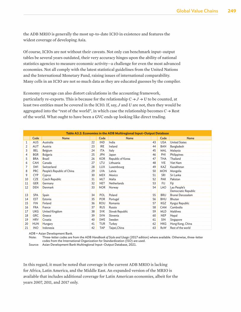
Global Value Chains
249Global Value Chains
the ADB MRIO is generally the most up-to-date ICIO in existence and features the widest coverage of developing Asia.
Of course, ICIOs are not without their caveats. Not only can benchmark input–output tables be several years outdated, their very accuracy hinges upon the ability of national statistics agencies to measure economic activity—a challenge for even the most advanced economies. Not all comply with the latest statistical guidelines from the United Nations and the International Monetary Fund, raising issues of international comparability. Many cells in an ICIO are not so much data as they are educated guesses by the compiler.
Economy coverage can also distort calculations in the accounting framework, particularly re-exports. This is because for the relationship C • J • U to be counted, at least two entities must be covered in the ICIO. If, say, J and U are not, then they would be aggregated into the “rest of the world”, in which case the relationship becomes C • Rest of the world. What ought to have been a GVC ends up looking like direct trading.
Table A3.2: Economies in the ADB Multiregional Input–Output DatabaseCode Name Code Name Code Name
1 AUS Australia 22 IND India 43 USA United States2 AUT Austria 23 IRE Ireland 44 BAN Bangladesh3 BEL Belgium 24 ITA Italy 45 MAL Malaysia4 BGR Bulgaria 25 JPN Japan 46 PHI Philippines5 BRA Brazil 26 KOR Republic of Korea 47 THA Thailand6 CAN Canada 27 LTU Lithuania 48 VIE Viet Nam7 SWI Switzerland 28 LUX Luxembourg 49 KAZ Kazakhstan8 PRC People’s Republic of China 29 LVA Latvia 50 MON Mongolia9 CYP Cyprus 30 MEX Mexico 51 SRI Sri Lanka
10 CZE Czech Republic 31 MLT Malta 52 PAK Pakistan11 GER Germany 32 NET Netherlands 53 FIJ Fiji12 DEN Denmark 33 NOR Norway 54 LAO Lao People’s
Democratic Republic13 SPA Spain 34 POL Poland 55 BRU Brunei Darussalam14 EST Estonia 35 POR Portugal 56 BHU Bhutan15 FIN Finland 36 ROU Romania 57 KGZ Kyrgyz Republic16 FRA France 37 RUS Russia 58 CAM Cambodia17 UKG United Kingdom 38 SVK Slovak Republic 59 MLD Maldives18 GRC Greece 39 SVN Slovenia 60 NEP Nepal19 HRV Croatia 40 SWE Sweden 61 SIN Singapore20 HUN Hungary 41 TUR Turkey 62 HKG Hong Kong, China21 INO Indonesia 42 TAP Taipei,China 63 RoW Rest of the world
ADB = Asian Development Bank.Note: Three-letter codes are from the ADB Handbook of Style and Usage (2017 edition) where available. Otherwise, three-letter
codes from the International Organization for Standardization (ISO) are used.Source: Asian Development Bank Multiregional Input–Output Database, 2021.
In this regard, it must be noted that coverage in the current ADB MRIO is lacking for Africa, Latin America, and the Middle East. An expanded version of the MRIO is available that includes additional coverage for Latin American economies, albeit for the years 2007, 2011, and 2017 only.
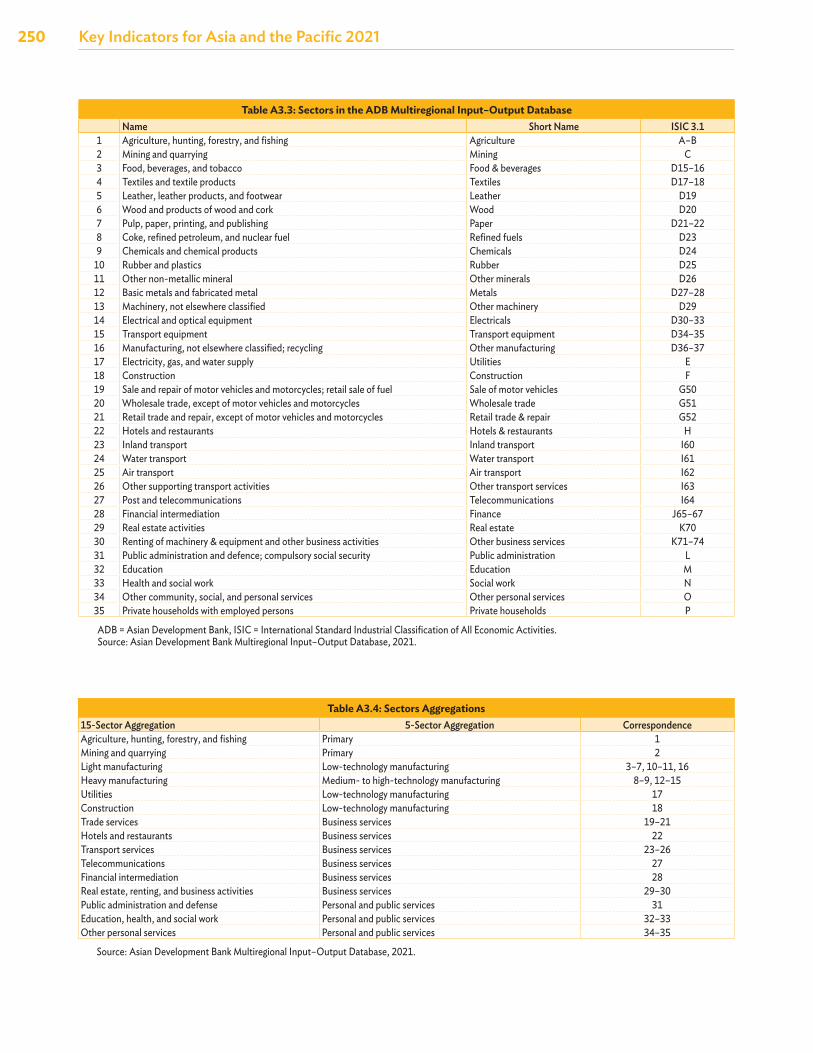
250 Key Indicators for Asia and the Pacific 2021
Table A3.3: Sectors in the ADB Multiregional Input–Output DatabaseName Short Name ISIC 3.1
1 Agriculture, hunting, forestry, and fishing Agriculture A–B2 Mining and quarrying Mining C3 Food, beverages, and tobacco Food & beverages D15–164 Textiles and textile products Textiles D17–185 Leather, leather products, and footwear Leather D196 Wood and products of wood and cork Wood D207 Pulp, paper, printing, and publishing Paper D21–228 Coke, refined petroleum, and nuclear fuel Refined fuels D239 Chemicals and chemical products Chemicals D24
10 Rubber and plastics Rubber D2511 Other non-metallic mineral Other minerals D2612 Basic metals and fabricated metal Metals D27–2813 Machinery, not elsewhere classified Other machinery D2914 Electrical and optical equipment Electricals D30–3315 Transport equipment Transport equipment D34–3516 Manufacturing, not elsewhere classified; recycling Other manufacturing D36–3717 Electricity, gas, and water supply Utilities E18 Construction Construction F19 Sale and repair of motor vehicles and motorcycles; retail sale of fuel Sale of motor vehicles G5020 Wholesale trade, except of motor vehicles and motorcycles Wholesale trade G5121 Retail trade and repair, except of motor vehicles and motorcycles Retail trade & repair G5222 Hotels and restaurants Hotels & restaurants H23 Inland transport Inland transport I6024 Water transport Water transport I6125 Air transport Air transport I6226 Other supporting transport activities Other transport services I6327 Post and telecommunications Telecommunications I6428 Financial intermediation Finance J65–6729 Real estate activities Real estate K7030 Renting of machinery & equipment and other business activities Other business services K71–7431 Public administration and defence; compulsory social security Public administration L32 Education Education M33 Health and social work Social work N34 Other community, social, and personal services Other personal services O35 Private households with employed persons Private households P
ADB = Asian Development Bank, ISIC = International Standard Industrial Classification of All Economic Activities.Source: Asian Development Bank Multiregional Input–Output Database, 2021.
Table A3.4: Sectors Aggregations15-Sector Aggregation 5-Sector Aggregation CorrespondenceAgriculture, hunting, forestry, and fishing Primary 1Mining and quarrying Primary 2Light manufacturing Low-technology manufacturing 3–7, 10–11, 16Heavy manufacturing Medium- to high-technology manufacturing 8–9, 12–15Utilities Low-technology manufacturing 17Construction Low-technology manufacturing 18Trade services Business services 19–21Hotels and restaurants Business services 22Transport services Business services 23–26Telecommunications Business services 27Financial intermediation Business services 28Real estate, renting, and business activities Business services 29–30Public administration and defense Personal and public services 31Education, health, and social work Personal and public services 32–33Other personal services Personal and public services 34–35
Source: Asian Development Bank Multiregional Input–Output Database, 2021.

Global Value Chains
251Global Value Chains
Summary
This appendix has covered the various conventions and approaches to GVC analysis used in the Key Indicators for Asia and the Pacific and various other ADB publications. Its major preoccupation is characterizing the different types of value-added trade masked by gross export statistics. To this end, exports are decomposed into five main categories: domestic value-added directly absorbed (DAVAX), domestic value-added re- exported and absorbed abroad (REX), domestic value-added re-exported and brought back home (REF), foreign value-added (FVA), and pure double-counting (PDC). These terms form the core of GVC analysis. Their relative shares, their individual trends, and their sector make-up all reveal something about the exporting economy’s GVC engagement. They may also be used to calculate associated indicators, including the GVC participation rate and the value-added-adjusted revealed comparative advantage index.
On a final note, it should be emphasized that the inclusion or exclusion of certain approaches in this framework is not intended as an argument over their validity, usefulness, or importance. The objective is merely to provide a coherent framework that best suits the needs of this publication and its users. Indeed, the framework has been kept relatively sparse to allow for flexibility in incorporating other methodologies as the need arises.
252 Key Indicators for Asia and the Pacific 2021
References
Asian Development Bank (ADB). 2015. Key Indicators for Asia and the Pacific 2015. Manila, Philippines: Asian Development Bank.
B. Balassa. 1965. Trade Liberalisation and “Revealed” Comparative Advantage. The Manchester School. 33 (2). pp. 99–123.
A. Borin and M. Mancini. 2019. Measuring What Matters in Global Value Chains and Value-Added Trade. Policy Research Working Paper No. 8804. Washington, DC: World Bank.
S. Giglioli, G. Giovannetti, E. Marvasi, and A. Vivoli. 2021. The Resilience of Global Value Chains During the Covid-19 Pandemic: The Case of Italy. UniFI DISEI Working Paper No. 07/2021. Florence, Italy: Università degli Studi Firenze Dipartimento di Scienze per L’Economia e L’Impresa.
D. Hummels, J. Ishii, and K. M. Yi. 2001. The Nature and Growth of Vertical Specialization in World Trade. Journal of International Economics. 54. pp. 75–96.
S. Inomata. 2017. Analytical Frameworks for Global Value Chains: An Overview. In World Bank, Global Value Chain Development Report 2017: Measuring and Analyzing the Impact of GVCs on Economic Development. pp. 15–35. Washington, DC: World Bank.
International Monetary Fund (IMF). 2019. World Economic Outlook: Global Manufacturing Downturn, Rising Trade Barriers. Washington, DC: International Monetary Fund.
IMF. 2021. World Economic Outlook: Managing Divergent Recoveries. Washington, DC: International Monetary Fund.
R. C. Johnson and G. Noguera. 2012. Accounting for Intermediates: Production Sharing and Trade in Value Added. Journal of International Economics. 86. pp. 224–236.
R. Koopman, Z. Wang, and S. J. Wei. 2014. Tracing Value-Added and Double Counting in Gross Exports. American Economic Review. 104 (2). pp. 459–494.
R. E. Miller and P. D. Blair. 2009. Input–Output Analysis: Foundations and Extensions (2nd ed.). Cambridge, UK: Cambridge University Press.
Organisation for Economic Co-operation and Development (OECD). 2021. Global Value Chains: Efficiency and Risks in the Context of COVID-19. Paris, France: Organisation for Economic Co-operation and Development.
M. P. Timmer, E. Dietzenbacher, B. Los, R. Stehrer, and G. J. de Vries. 2015. An Illustrated User Guide to the World Input–Output Database: The Case of Global Automotive Production. Review of International Economics. 23 (3). pp. 575–605.
Z. Wang, S. J. Wei, X. Yu, and K. Zhu. 2017. Measures of Participation in Global Value Chains and Global Business Cycles. NBER Working Paper No. 23222. Cambridge, MA: National Bureau of Economic Research.
Z. Wang, S. J. Wei, and K. Zhu. 2018. Quantifying International Production Sharing at the Bilateral and Sector Levels. NBER Working Paper No. 19677. Cambridge, MA: National Bureau of Economic Research.
World Bank. 2020. Global Economic Prospects: Slow Growth, Policy Challenges (January 2020). Washington, DC: World Bank.
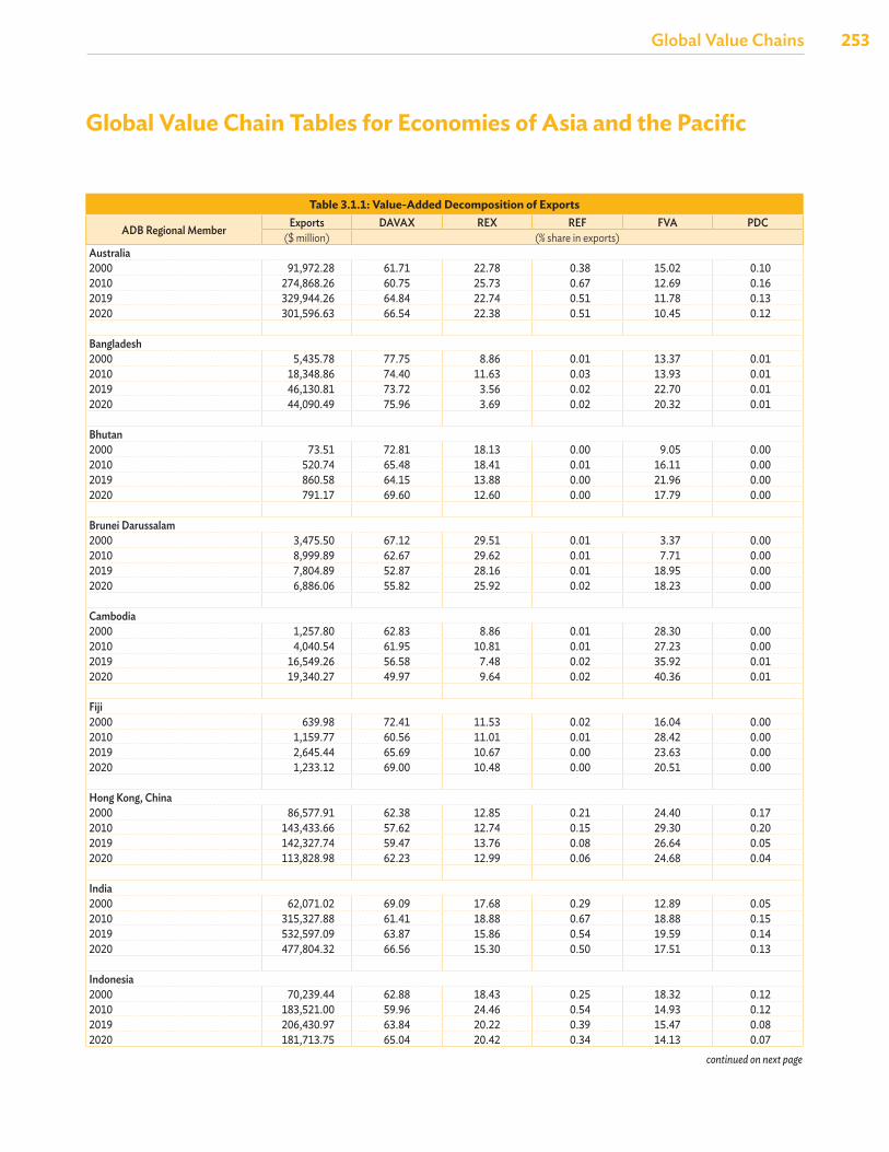
Global Value Chains
253Global Value Chains
Global Value Chain Tables for Economies of Asia and the Pacific
Table 3.1.1: Value-Added Decomposition of Exports
ADB Regional Member Exports DAVAX REX REF FVA PDC($ million) (% share in exports)
Australia2000 91,972.28 61.71 22.78 0.38 15.02 0.102010 274,868.26 60.75 25.73 0.67 12.69 0.162019 329,944.26 64.84 22.74 0.51 11.78 0.132020 301,596.63 66.54 22.38 0.51 10.45 0.12
Bangladesh2000 5,435.78 77.75 8.86 0.01 13.37 0.012010 18,348.86 74.40 11.63 0.03 13.93 0.012019 46,130.81 73.72 3.56 0.02 22.70 0.012020 44,090.49 75.96 3.69 0.02 20.32 0.01
Bhutan2000 73.51 72.81 18.13 0.00 9.05 0.002010 520.74 65.48 18.41 0.01 16.11 0.002019 860.58 64.15 13.88 0.00 21.96 0.002020 791.17 69.60 12.60 0.00 17.79 0.00
Brunei Darussalam2000 3,475.50 67.12 29.51 0.01 3.37 0.002010 8,999.89 62.67 29.62 0.01 7.71 0.002019 7,804.89 52.87 28.16 0.01 18.95 0.002020 6,886.06 55.82 25.92 0.02 18.23 0.00
Cambodia2000 1,257.80 62.83 8.86 0.01 28.30 0.002010 4,040.54 61.95 10.81 0.01 27.23 0.002019 16,549.26 56.58 7.48 0.02 35.92 0.012020 19,340.27 49.97 9.64 0.02 40.36 0.01
Fiji2000 639.98 72.41 11.53 0.02 16.04 0.002010 1,159.77 60.56 11.01 0.01 28.42 0.002019 2,645.44 65.69 10.67 0.00 23.63 0.002020 1,233.12 69.00 10.48 0.00 20.51 0.00
Hong Kong, China2000 86,577.91 62.38 12.85 0.21 24.40 0.172010 143,433.66 57.62 12.74 0.15 29.30 0.202019 142,327.74 59.47 13.76 0.08 26.64 0.052020 113,828.98 62.23 12.99 0.06 24.68 0.04
India2000 62,071.02 69.09 17.68 0.29 12.89 0.052010 315,327.88 61.41 18.88 0.67 18.88 0.152019 532,597.09 63.87 15.86 0.54 19.59 0.142020 477,804.32 66.56 15.30 0.50 17.51 0.13
Indonesia2000 70,239.44 62.88 18.43 0.25 18.32 0.122010 183,521.00 59.96 24.46 0.54 14.93 0.122019 206,430.97 63.84 20.22 0.39 15.47 0.082020 181,713.75 65.04 20.42 0.34 14.13 0.07
continued on next page
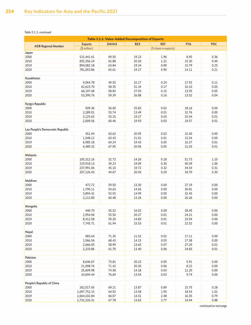
254 Key Indicators for Asia and the Pacific 2021
Table 3.1.1: Value-Added Decomposition of Exports
ADB Regional Member Exports DAVAX REX REF FVA PDC($ million) (% share in exports)
Japan2000 515,441.61 69.50 19.23 1.96 8.95 0.362010 835,356.24 62.88 20.20 1.22 15.30 0.402019 894,082.18 63.84 19.24 0.89 15.79 0.252020 781,053.86 65.61 19.17 0.90 14.11 0.21
Kazakhstan2000 9,064.78 49.55 32.17 0.24 17.92 0.112010 62,623.70 58.35 31.34 0.17 10.10 0.052019 66,197.68 58.83 27.03 0.15 13.95 0.052020 53,390.76 59.39 26.88 0.16 13.52 0.04
Kyrgyz Republic2000 509.36 56.00 25.82 0.02 18.16 0.002010 2,289.01 53.74 13.49 0.01 32.76 0.002019 3,125.63 55.15 19.27 0.03 25.54 0.012020 2,009.56 60.46 19.93 0.03 19.57 0.01
Lao People’s Democratic Republic2000 451.94 63.62 20.95 0.02 15.40 0.002010 1,548.12 63.43 21.01 0.01 15.54 0.002019 6,985.18 64.24 19.43 0.05 16.27 0.012020 6,489.32 67.95 20.96 0.05 11.03 0.01
Malaysia2000 105,312.16 32.72 14.26 0.18 51.73 1.102010 219,918.13 39.23 19.09 0.30 40.39 1.002019 237,991.06 45.10 19.72 0.32 34.54 0.312020 207,126.43 44.67 20.04 0.29 34.70 0.30
Maldives2000 472.72 59.50 13.30 0.00 27.19 0.002010 1,790.11 54.63 14.56 0.00 30.81 0.002019 3,894.41 52.55 14.99 0.00 32.45 0.002020 2,112.80 60.48 13.26 0.00 26.26 0.00
Mongolia2000 440.70 55.52 16.02 0.00 28.45 0.002010 2,954.96 55.50 20.27 0.01 24.21 0.002019 8,412.58 59.20 14.85 0.01 25.94 0.002020 7,745.71 61.94 15.53 0.01 22.52 0.00
Nepal2000 983.64 71.35 11.52 0.02 17.11 0.002010 1,066.56 68.43 14.15 0.03 17.38 0.002019 2,666.05 58.99 13.65 0.07 27.29 0.012020 2,233.86 61.70 13.40 0.06 24.83 0.01
Pakistan2000 8,646.67 73.81 20.23 0.05 5.91 0.002010 21,098.76 71.42 20.30 0.06 8.22 0.002019 25,609.98 74.58 14.18 0.03 11.20 0.002020 24,694.44 76.69 13.54 0.03 9.74 0.00
People’s Republic of China2000 262,017.65 69.21 13.87 0.89 15.75 0.282010 1,697,752.15 64.92 13.58 1.95 18.54 1.012019 2,664,102.84 66.07 14.31 2.48 16.35 0.792020 2,732,326.31 67.78 13.63 2.77 14.94 0.88
Table 3.1.1: continued
continued on next page
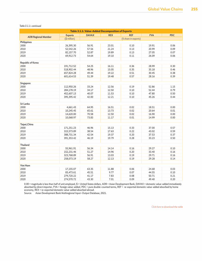
Global Value Chains
255Global Value Chains
Table 3.1.1: Value-Added Decomposition of Exports
ADB Regional Member Exports DAVAX REX REF FVA PDC($ million) (% share in exports)
Philippines2000 26,395.30 56.91 23.01 0.10 19.91 0.062010 52,542.26 57.56 21.24 0.13 20.99 0.092019 82,157.70 52.87 19.89 0.13 27.05 0.072020 69,912.73 54.64 19.10 0.11 26.09 0.06
Republic of Korea2000 191,712.52 54.25 16.11 0.36 28.99 0.302010 518,902.44 48.96 15.05 0.35 35.18 0.462019 657,824.28 49.44 19.22 0.51 30.45 0.382020 601,614.53 51.39 19.48 0.57 28.16 0.39
Singapore2000 112,950.26 33.24 12.56 0.19 52.86 1.152010 284,178.19 34.17 12.50 0.10 52.44 0.792019 452,607.13 40.07 11.53 0.10 47.80 0.502020 395,395.42 42.00 12.21 0.10 45.26 0.44
Sri Lanka2000 4,661.43 64.95 16.51 0.02 18.51 0.002010 10,245.45 65.61 13.73 0.02 20.64 0.012019 14,620.00 70.58 12.50 0.02 16.90 0.002020 10,068.97 73.83 11.17 0.01 14.99 0.00
Taipei,China2000 171,251.23 46.96 15.13 0.33 37.00 0.572010 315,573.89 38.54 17.63 0.22 43.02 0.592019 388,731.34 42.54 19.37 0.20 37.53 0.372020 391,353.42 46.19 19.79 0.28 33.23 0.50
Thailand2000 55,961.91 56.34 14.14 0.16 29.27 0.102010 152,231.46 51.27 14.96 0.20 33.40 0.162019 323,768.89 56.91 13.03 0.19 29.71 0.162020 258,073.19 58.27 12.13 0.19 29.28 0.14
Viet Nam2000 17,155.07 63.35 11.88 0.06 24.68 0.032010 83,473.61 45.51 9.77 0.07 44.55 0.102019 279,720.22 41.17 7.83 0.08 50.71 0.212020 274,570.72 43.30 7.01 0.09 49.40 0.20
0.00 = magnitude is less than half of unit employed, $ = United States dollars, ADB = Asian Development Bank, DAVAX = domestic value-added immediately absorbed by direct importer, FVA = foreign value-added, PDC = pure double-counted terms, REF = re-exported domestic value-added absorbed by home economy, REX = re-exported domestic value-added absorbed abroad.Source: Asian Development Bank Multiregional Input–Output Database, 2021.
Table 3.1.1: continued
Click here to download the table
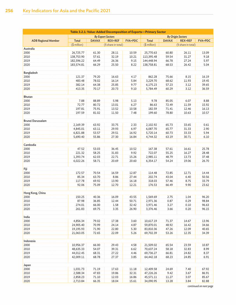
256 Key Indicators for Asia and the Pacific 2021
Table 3.2.1: Value-Added Decomposition of Exports—Primary Sector
ADB Regional MemberBy Export Sectors By Origin Sectors
Total DAVAX REX+REF FVA+PDC Total DAVAX REX+REF FVA+PDC($ million) (% share in total) ($ million) (% share in total)
Australia2000 26,725.77 61.30 28.11 10.59 25,770.63 60.80 26.11 13.092010 138,753.90 57.61 32.19 10.21 113,395.48 59.54 31.27 9.182019 182,596.22 64.49 26.36 9.15 144,448.94 66.78 27.24 5.972020 183,574.81 66.29 25.50 8.22 138,758.81 68.53 26.42 5.04
Bangladesh2000 121.37 79.20 16.63 4.17 862.28 75.66 8.15 16.192010 483.48 78.02 16.14 5.84 3,229.70 68.62 11.93 19.452019 382.14 64.38 25.85 9.77 6,175.23 57.23 3.12 39.652020 413.35 70.17 20.73 9.10 5,784.49 60.29 3.12 36.59
Bhutan2000 7.88 88.89 5.98 5.13 9.78 85.05 6.07 8.882010 72.77 80.72 13.01 6.27 86.63 72.49 11.59 15.922019 197.81 75.91 13.52 10.58 182.59 71.41 12.46 16.132020 197.59 81.02 11.50 7.48 199.60 78.80 10.63 10.57
Brunei Darussalam2000 2,169.39 63.92 33.75 2.33 2,102.92 65.73 33.65 0.612010 4,845.01 63.11 29.93 6.97 6,087.70 65.77 31.33 2.902019 6,821.88 53.57 29.51 16.92 5,720.14 60.73 33.33 5.942020 5,690.40 55.86 27.30 16.84 4,744.32 63.19 30.71 6.10
Cambodia2000 47.52 53.03 36.45 10.52 167.38 57.61 16.61 25.782010 221.32 58.25 31.83 9.92 722.07 55.25 16.27 28.482019 1,393.74 62.03 22.71 15.26 2,985.11 48.79 13.73 37.482020 6,022.26 58.71 20.69 20.60 6,354.17 54.24 19.06 26.70
Fiji2000 172.57 70.54 16.59 12.87 114.48 72.85 12.71 14.442010 85.34 63.70 8.86 27.44 202.74 43.04 6.40 50.562019 117.78 69.92 13.90 16.18 318.03 57.46 8.75 33.792020 92.06 75.09 12.70 12.21 176.53 66.49 9.90 23.62
Hong Kong, China2000 150.25 40.36 16.09 43.55 1,569.69 2.75 1.04 96.202010 87.98 36.85 12.44 50.71 2,971.36 0.87 0.29 98.842019 274.01 66.00 1.58 32.42 3,971.46 3.27 0.10 96.632020 261.83 69.75 3.35 26.90 3,376.46 3.66 0.20 96.15
India2000 4,856.34 79.02 17.38 3.60 10,617.19 71.37 14.67 13.962010 24,905.40 70.99 24.14 4.87 59,870.01 48.92 16.42 34.662019 19,195.93 71.90 22.80 5.30 83,810.36 47.26 12.09 40.652020 21,063.05 72.65 22.09 5.26 69,702.39 53.26 12.35 34.39
Indonesia2000 10,956.37 66.00 29.43 4.58 21,509.02 65.54 23.59 10.872010 48,635.33 54.07 39.31 6.62 70,637.24 58.18 32.83 8.992019 44,012.45 68.31 27.22 4.46 69,736.27 66.81 24.82 8.372020 42,009.11 68.78 27.37 3.85 64,442.18 68.23 24.85 6.91
Japan2000 1,031.73 71.19 17.63 11.18 12,409.58 24.69 7.40 67.922010 2,588.34 47.83 19.86 32.31 47,226.26 9.42 3.67 86.912019 2,858.23 71.10 12.03 16.86 45,571.11 11.27 3.07 85.672020 2,713.84 66.35 18.04 15.61 34,090.95 13.28 3.84 82.88
continued on next page
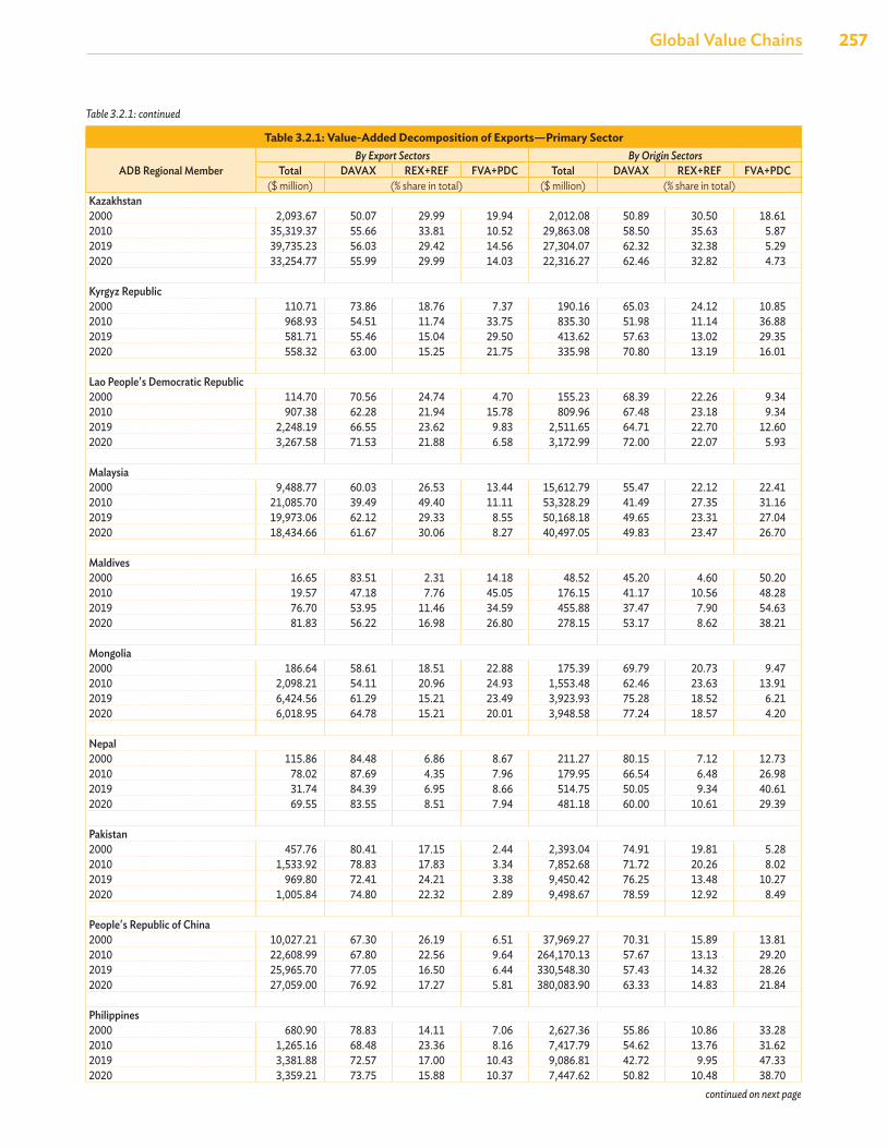
Global Value Chains
257Global Value Chains
Table 3.2.1: Value-Added Decomposition of Exports—Primary Sector
ADB Regional MemberBy Export Sectors By Origin Sectors
Total DAVAX REX+REF FVA+PDC Total DAVAX REX+REF FVA+PDC($ million) (% share in total) ($ million) (% share in total)
Kazakhstan2000 2,093.67 50.07 29.99 19.94 2,012.08 50.89 30.50 18.612010 35,319.37 55.66 33.81 10.52 29,863.08 58.50 35.63 5.872019 39,735.23 56.03 29.42 14.56 27,304.07 62.32 32.38 5.292020 33,254.77 55.99 29.99 14.03 22,316.27 62.46 32.82 4.73
Kyrgyz Republic2000 110.71 73.86 18.76 7.37 190.16 65.03 24.12 10.852010 968.93 54.51 11.74 33.75 835.30 51.98 11.14 36.882019 581.71 55.46 15.04 29.50 413.62 57.63 13.02 29.352020 558.32 63.00 15.25 21.75 335.98 70.80 13.19 16.01
Lao People's Democratic Republic2000 114.70 70.56 24.74 4.70 155.23 68.39 22.26 9.342010 907.38 62.28 21.94 15.78 809.96 67.48 23.18 9.342019 2,248.19 66.55 23.62 9.83 2,511.65 64.71 22.70 12.602020 3,267.58 71.53 21.88 6.58 3,172.99 72.00 22.07 5.93
Malaysia2000 9,488.77 60.03 26.53 13.44 15,612.79 55.47 22.12 22.412010 21,085.70 39.49 49.40 11.11 53,328.29 41.49 27.35 31.162019 19,973.06 62.12 29.33 8.55 50,168.18 49.65 23.31 27.042020 18,434.66 61.67 30.06 8.27 40,497.05 49.83 23.47 26.70
Maldives2000 16.65 83.51 2.31 14.18 48.52 45.20 4.60 50.202010 19.57 47.18 7.76 45.05 176.15 41.17 10.56 48.282019 76.70 53.95 11.46 34.59 455.88 37.47 7.90 54.632020 81.83 56.22 16.98 26.80 278.15 53.17 8.62 38.21
Mongolia2000 186.64 58.61 18.51 22.88 175.39 69.79 20.73 9.472010 2,098.21 54.11 20.96 24.93 1,553.48 62.46 23.63 13.912019 6,424.56 61.29 15.21 23.49 3,923.93 75.28 18.52 6.212020 6,018.95 64.78 15.21 20.01 3,948.58 77.24 18.57 4.20
Nepal2000 115.86 84.48 6.86 8.67 211.27 80.15 7.12 12.732010 78.02 87.69 4.35 7.96 179.95 66.54 6.48 26.982019 31.74 84.39 6.95 8.66 514.75 50.05 9.34 40.612020 69.55 83.55 8.51 7.94 481.18 60.00 10.61 29.39
Pakistan2000 457.76 80.41 17.15 2.44 2,393.04 74.91 19.81 5.282010 1,533.92 78.83 17.83 3.34 7,852.68 71.72 20.26 8.022019 969.80 72.41 24.21 3.38 9,450.42 76.25 13.48 10.272020 1,005.84 74.80 22.32 2.89 9,498.67 78.59 12.92 8.49
People's Republic of China2000 10,027.21 67.30 26.19 6.51 37,969.27 70.31 15.89 13.812010 22,608.99 67.80 22.56 9.64 264,170.13 57.67 13.13 29.202019 25,965.70 77.05 16.50 6.44 330,548.30 57.43 14.32 28.262020 27,059.00 76.92 17.27 5.81 380,083.90 63.33 14.83 21.84
Philippines2000 680.90 78.83 14.11 7.06 2,627.36 55.86 10.86 33.282010 1,265.16 68.48 23.36 8.16 7,417.79 54.62 13.76 31.622019 3,381.88 72.57 17.00 10.43 9,086.81 42.72 9.95 47.332020 3,359.21 73.75 15.88 10.37 7,447.62 50.82 10.48 38.70
Table 3.2.1: continued
continued on next page
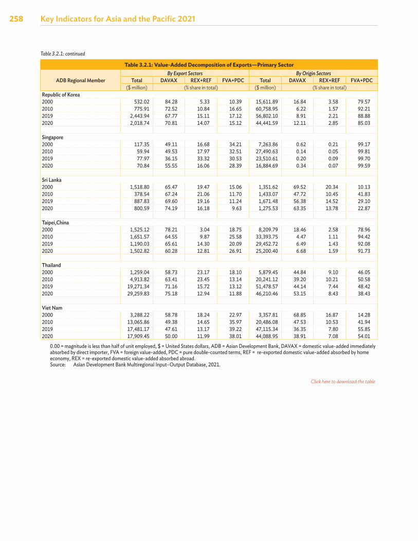
258 Key Indicators for Asia and the Pacific 2021
Table 3.2.1: Value-Added Decomposition of Exports—Primary Sector
ADB Regional MemberBy Export Sectors By Origin Sectors
Total DAVAX REX+REF FVA+PDC Total DAVAX REX+REF FVA+PDC($ million) (% share in total) ($ million) (% share in total)
Republic of Korea2000 532.02 84.28 5.33 10.39 15,611.89 16.84 3.58 79.572010 775.91 72.52 10.84 16.65 60,758.95 6.22 1.57 92.212019 2,443.94 67.77 15.11 17.12 56,802.10 8.91 2.21 88.882020 2,018.74 70.81 14.07 15.12 44,441.59 12.11 2.85 85.03
Singapore2000 117.35 49.11 16.68 34.21 7,263.86 0.62 0.21 99.172010 59.94 49.53 17.97 32.51 27,490.63 0.14 0.05 99.812019 77.97 36.15 33.32 30.53 23,510.61 0.20 0.09 99.702020 70.84 55.55 16.06 28.39 16,884.69 0.34 0.07 99.59
Sri Lanka2000 1,518.80 65.47 19.47 15.06 1,351.62 69.52 20.34 10.132010 378.54 67.24 21.06 11.70 1,433.07 47.72 10.45 41.832019 887.83 69.60 19.16 11.24 1,671.48 56.38 14.52 29.102020 800.59 74.19 16.18 9.63 1,275.53 63.35 13.78 22.87
Taipei,China2000 1,525.12 78.21 3.04 18.75 8,209.79 18.46 2.58 78.962010 1,651.57 64.55 9.87 25.58 33,393.75 4.47 1.11 94.422019 1,190.03 65.61 14.30 20.09 29,452.72 6.49 1.43 92.082020 1,502.82 60.28 12.81 26.91 25,200.40 6.68 1.59 91.73
Thailand2000 1,259.04 58.73 23.17 18.10 5,879.45 44.84 9.10 46.052010 4,913.82 63.41 23.45 13.14 20,241.12 39.20 10.21 50.582019 19,271.34 71.16 15.72 13.12 51,478.57 44.14 7.44 48.422020 29,259.83 75.18 12.94 11.88 46,210.46 53.15 8.43 38.43
Viet Nam2000 3,288.22 58.78 18.24 22.97 3,357.81 68.85 16.87 14.282010 13,065.86 49.38 14.65 35.97 20,486.08 47.53 10.53 41.942019 17,481.17 47.61 13.17 39.22 47,115.34 36.35 7.80 55.852020 17,909.45 50.00 11.99 38.01 44,088.95 38.91 7.08 54.01
0.00 = magnitude is less than half of unit employed, $ = United States dollars, ADB = Asian Development Bank, DAVAX = domestic value-added immediately absorbed by direct importer, FVA = foreign value-added, PDC = pure double-counted terms, REF = re-exported domestic value-added absorbed by home economy, REX = re-exported domestic value-added absorbed abroad.Source: Asian Development Bank Multiregional Input–Output Database, 2021.
Table 3.2.1: continued
Click here to download the table
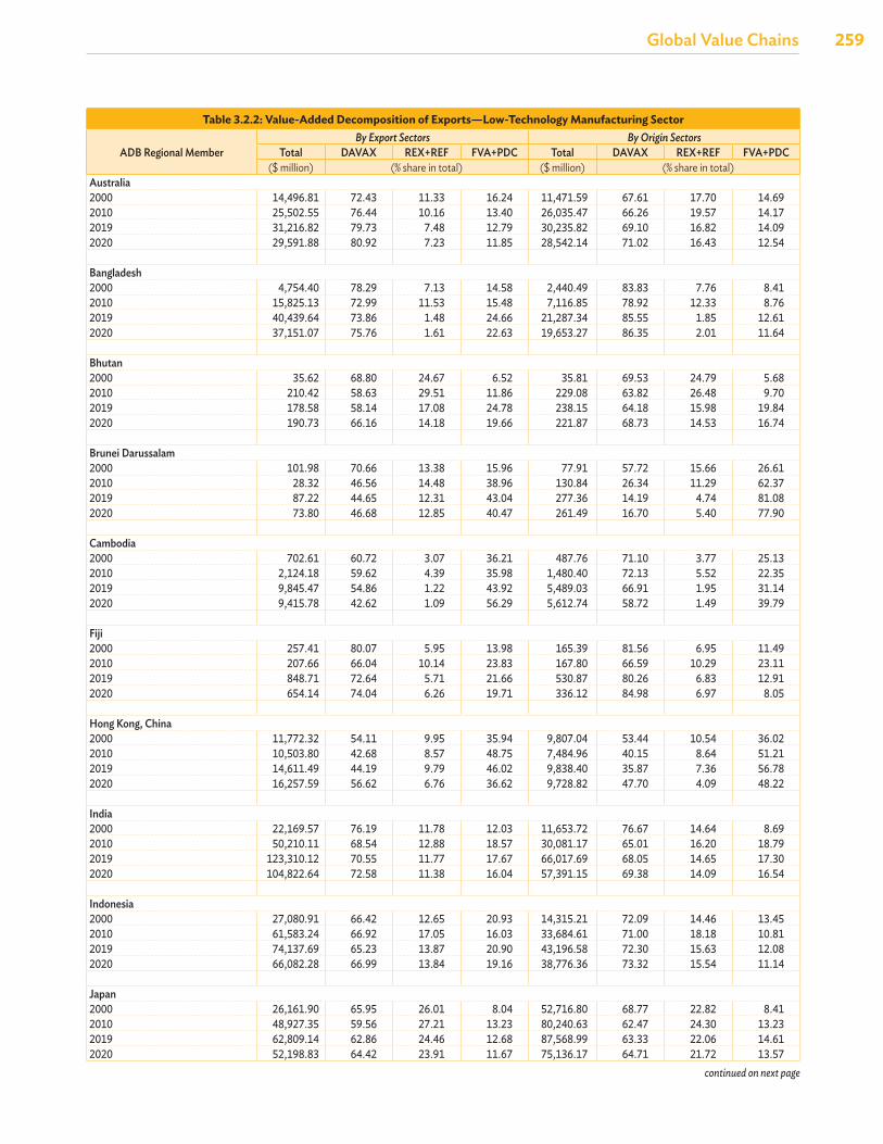
Global Value Chains
259Global Value Chains
Table 3.2.2: Value-Added Decomposition of Exports—Low-Technology Manufacturing Sector
ADB Regional MemberBy Export Sectors By Origin Sectors
Total DAVAX REX+REF FVA+PDC Total DAVAX REX+REF FVA+PDC($ million) (% share in total) ($ million) (% share in total)
Australia2000 14,496.81 72.43 11.33 16.24 11,471.59 67.61 17.70 14.692010 25,502.55 76.44 10.16 13.40 26,035.47 66.26 19.57 14.172019 31,216.82 79.73 7.48 12.79 30,235.82 69.10 16.82 14.092020 29,591.88 80.92 7.23 11.85 28,542.14 71.02 16.43 12.54
Bangladesh2000 4,754.40 78.29 7.13 14.58 2,440.49 83.83 7.76 8.412010 15,825.13 72.99 11.53 15.48 7,116.85 78.92 12.33 8.762019 40,439.64 73.86 1.48 24.66 21,287.34 85.55 1.85 12.612020 37,151.07 75.76 1.61 22.63 19,653.27 86.35 2.01 11.64
Bhutan2000 35.62 68.80 24.67 6.52 35.81 69.53 24.79 5.682010 210.42 58.63 29.51 11.86 229.08 63.82 26.48 9.702019 178.58 58.14 17.08 24.78 238.15 64.18 15.98 19.842020 190.73 66.16 14.18 19.66 221.87 68.73 14.53 16.74
Brunei Darussalam2000 101.98 70.66 13.38 15.96 77.91 57.72 15.66 26.612010 28.32 46.56 14.48 38.96 130.84 26.34 11.29 62.372019 87.22 44.65 12.31 43.04 277.36 14.19 4.74 81.082020 73.80 46.68 12.85 40.47 261.49 16.70 5.40 77.90
Cambodia2000 702.61 60.72 3.07 36.21 487.76 71.10 3.77 25.132010 2,124.18 59.62 4.39 35.98 1,480.40 72.13 5.52 22.352019 9,845.47 54.86 1.22 43.92 5,489.03 66.91 1.95 31.142020 9,415.78 42.62 1.09 56.29 5,612.74 58.72 1.49 39.79
Fiji2000 257.41 80.07 5.95 13.98 165.39 81.56 6.95 11.492010 207.66 66.04 10.14 23.83 167.80 66.59 10.29 23.112019 848.71 72.64 5.71 21.66 530.87 80.26 6.83 12.912020 654.14 74.04 6.26 19.71 336.12 84.98 6.97 8.05
Hong Kong, China2000 11,772.32 54.11 9.95 35.94 9,807.04 53.44 10.54 36.022010 10,503.80 42.68 8.57 48.75 7,484.96 40.15 8.64 51.212019 14,611.49 44.19 9.79 46.02 9,838.40 35.87 7.36 56.782020 16,257.59 56.62 6.76 36.62 9,728.82 47.70 4.09 48.22
India2000 22,169.57 76.19 11.78 12.03 11,653.72 76.67 14.64 8.692010 50,210.11 68.54 12.88 18.57 30,081.17 65.01 16.20 18.792019 123,310.12 70.55 11.77 17.67 66,017.69 68.05 14.65 17.302020 104,822.64 72.58 11.38 16.04 57,391.15 69.38 14.09 16.54
Indonesia2000 27,080.91 66.42 12.65 20.93 14,315.21 72.09 14.46 13.452010 61,583.24 66.92 17.05 16.03 33,684.61 71.00 18.18 10.812019 74,137.69 65.23 13.87 20.90 43,196.58 72.30 15.63 12.082020 66,082.28 66.99 13.84 19.16 38,776.36 73.32 15.54 11.14
Japan2000 26,161.90 65.95 26.01 8.04 52,716.80 68.77 22.82 8.412010 48,927.35 59.56 27.21 13.23 80,240.63 62.47 24.30 13.232019 62,809.14 62.86 24.46 12.68 87,568.99 63.33 22.06 14.612020 52,198.83 64.42 23.91 11.67 75,136.17 64.71 21.72 13.57
continued on next page
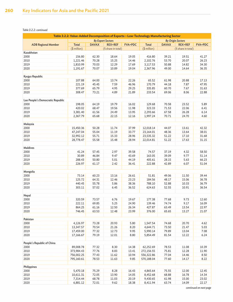
260 Key Indicators for Asia and the Pacific 2021
Table 3.2.2: Value-Added Decomposition of Exports—Low-Technology Manufacturing Sector
ADB Regional MemberBy Export Sectors By Origin Sectors
Total DAVAX REX+REF FVA+PDC Total DAVAX REX+REF FVA+PDC($ million) (% share in total) ($ million) (% share in total)
Kazakhstan2000 156.80 62.30 18.64 19.05 416.80 39.21 19.51 41.272010 1,221.46 70.28 15.25 14.46 2,102.76 53.70 20.07 26.232019 1,810.99 70.03 12.29 17.69 3,117.53 50.88 14.82 34.302020 1,191.67 70.07 10.89 19.04 2,367.96 49.00 14.64 36.35
Kyrgyz Republic2000 107.88 64.00 13.74 22.26 65.52 61.98 20.88 17.132010 221.19 45.45 7.59 46.96 170.79 44.18 7.87 47.952019 377.69 65.79 4.95 29.25 335.85 60.70 7.67 31.632020 308.47 73.21 4.89 21.89 233.54 69.06 8.06 22.88
Lao People's Democratic Republic2000 198.05 64.19 19.79 16.02 129.68 70.58 23.52 5.892010 420.02 68.47 19.56 11.98 323.33 71.53 22.06 6.412019 3,381.40 61.56 24.49 13.95 2,293.66 67.58 26.28 6.142020 2,367.79 65.68 22.15 12.16 1,997.24 70.71 24.70 4.60
Malaysia2000 15,450.36 50.28 11.74 37.99 12,018.14 44.07 13.61 42.322010 47,247.04 55.04 11.19 33.77 23,164.01 48.36 13.64 38.012019 32,992.12 55.71 15.33 28.96 23,535.32 51.22 17.10 31.682020 28,778.47 55.58 15.48 28.94 22,014.81 51.22 17.63 31.15
Maldives2000 41.24 57.45 2.97 39.58 74.57 37.19 4.32 58.502010 30.89 46.84 9.47 43.69 163.05 39.09 9.77 51.142019 288.43 50.80 5.01 44.19 405.61 28.15 5.63 66.232020 226.97 61.17 2.42 36.41 222.88 42.89 6.07 51.04
Mongolia2000 73.14 60.23 13.16 26.61 51.81 49.06 11.50 39.442010 125.72 64.31 12.46 23.23 184.56 48.17 15.06 36.782019 440.45 55.78 5.86 38.36 788.10 52.88 10.33 36.792020 303.11 57.02 6.45 36.52 624.63 52.55 10.91 36.54
Nepal2000 320.59 73.57 6.76 19.67 177.38 77.68 9.73 12.602010 222.11 69.85 5.25 24.90 139.46 74.74 9.17 16.092019 864.25 61.16 12.50 26.34 427.87 63.49 13.54 22.972020 746.45 63.53 12.48 23.99 376.00 65.65 13.27 21.07
Pakistan2000 4,126.97 73.28 20.93 5.80 1,547.54 74.68 20.70 4.622010 13,347.57 70.54 21.26 8.20 4,644.71 73.50 21.47 5.032019 17,459.00 77.32 12.73 9.95 5,990.14 79.89 13.04 7.082020 17,166.67 79.19 12.01 8.80 5,854.49 81.54 12.22 6.24
People's Republic of China2000 89,008.78 77.32 8.30 14.38 62,252.69 78.53 11.08 10.392010 373,984.43 77.76 8.83 13.41 272,156.55 75.81 12.28 11.902019 756,002.25 77.43 11.62 10.94 556,322.86 77.04 14.46 8.502020 795,160.61 78.53 11.63 9.85 570,188.04 77.60 14.17 8.22
Philippines2000 5,470.18 75.29 8.28 16.43 4,865.64 75.55 12.00 12.452010 10,611.31 72.05 13.90 14.05 8,452.68 68.88 16.78 14.342019 7,314.44 68.78 11.03 20.19 9,430.65 61.98 15.00 23.022020 6,881.12 72.01 9.62 18.38 8,411.94 63.74 14.09 22.17
continued on next page
Table 3.2.2: continued
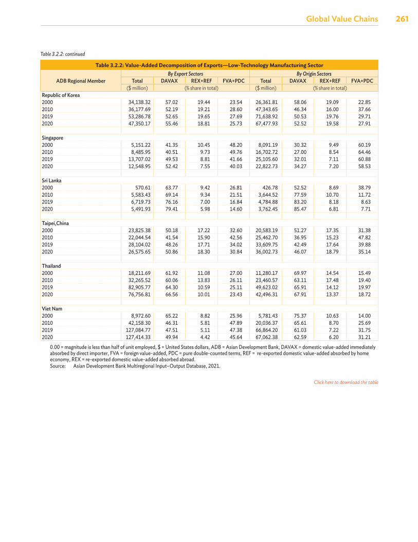
Global Value Chains
261Global Value Chains
Table 3.2.2: Value-Added Decomposition of Exports—Low-Technology Manufacturing Sector
ADB Regional MemberBy Export Sectors By Origin Sectors
Total DAVAX REX+REF FVA+PDC Total DAVAX REX+REF FVA+PDC($ million) (% share in total) ($ million) (% share in total)
Republic of Korea2000 34,138.32 57.02 19.44 23.54 26,361.81 58.06 19.09 22.852010 36,177.69 52.19 19.21 28.60 47,343.65 46.34 16.00 37.662019 53,286.78 52.65 19.65 27.69 71,638.92 50.53 19.76 29.712020 47,350.17 55.46 18.81 25.73 67,477.93 52.52 19.58 27.91
Singapore2000 5,151.22 41.35 10.45 48.20 8,091.19 30.32 9.49 60.192010 8,485.95 40.51 9.73 49.76 16,702.72 27.00 8.54 64.462019 13,707.02 49.53 8.81 41.66 25,105.60 32.01 7.11 60.882020 12,548.95 52.42 7.55 40.03 22,822.73 34.27 7.20 58.53
Sri Lanka2000 570.61 63.77 9.42 26.81 426.78 52.52 8.69 38.792010 5,583.43 69.14 9.34 21.51 3,644.52 77.59 10.70 11.722019 6,719.73 76.16 7.00 16.84 4,784.88 83.20 8.18 8.632020 5,491.93 79.41 5.98 14.60 3,762.45 85.47 6.81 7.71
Taipei,China2000 23,825.38 50.18 17.22 32.60 20,583.19 51.27 17.35 31.382010 22,044.54 41.54 15.90 42.56 25,462.70 36.95 15.23 47.822019 28,104.02 48.26 17.71 34.02 33,609.75 42.49 17.64 39.882020 26,575.65 50.86 18.30 30.84 36,002.73 46.07 18.79 35.14
Thailand2000 18,211.69 61.92 11.08 27.00 11,280.17 69.97 14.54 15.492010 32,265.52 60.06 13.83 26.11 23,460.57 63.11 17.48 19.402019 82,905.77 64.30 10.59 25.11 49,623.02 65.91 14.12 19.972020 76,756.81 66.56 10.01 23.43 42,496.31 67.91 13.37 18.72
Viet Nam2000 8,972.60 65.22 8.82 25.96 5,781.43 75.37 10.63 14.002010 42,158.30 46.31 5.81 47.89 20,036.37 65.61 8.70 25.692019 127,084.77 47.51 5.11 47.38 66,864.20 61.03 7.22 31.752020 127,414.33 49.94 4.42 45.64 67,062.38 62.59 6.20 31.21
0.00 = magnitude is less than half of unit employed, $ = United States dollars, ADB = Asian Development Bank, DAVAX = domestic value-added immediately absorbed by direct importer, FVA = foreign value-added, PDC = pure double-counted terms, REF = re-exported domestic value-added absorbed by home economy, REX = re-exported domestic value-added absorbed abroad.Source: Asian Development Bank Multiregional Input–Output Database, 2021.
Table 3.2.2: continued
Click here to download the table
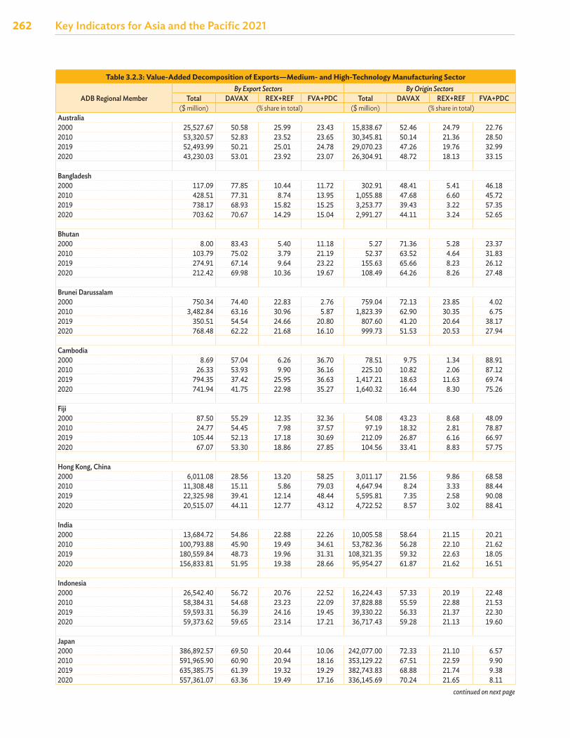
262 Key Indicators for Asia and the Pacific 2021
Table 3.2.3: Value-Added Decomposition of Exports—Medium- and High-Technology Manufacturing Sector
ADB Regional MemberBy Export Sectors By Origin Sectors
Total DAVAX REX+REF FVA+PDC Total DAVAX REX+REF FVA+PDC($ million) (% share in total) ($ million) (% share in total)
Australia2000 25,527.67 50.58 25.99 23.43 15,838.67 52.46 24.79 22.762010 53,320.57 52.83 23.52 23.65 30,345.81 50.14 21.36 28.502019 52,493.99 50.21 25.01 24.78 29,070.23 47.26 19.76 32.992020 43,230.03 53.01 23.92 23.07 26,304.91 48.72 18.13 33.15
Bangladesh2000 117.09 77.85 10.44 11.72 302.91 48.41 5.41 46.182010 428.51 77.31 8.74 13.95 1,055.88 47.68 6.60 45.722019 738.17 68.93 15.82 15.25 3,253.77 39.43 3.22 57.352020 703.62 70.67 14.29 15.04 2,991.27 44.11 3.24 52.65
Bhutan2000 8.00 83.43 5.40 11.18 5.27 71.36 5.28 23.372010 103.79 75.02 3.79 21.19 52.37 63.52 4.64 31.832019 274.91 67.14 9.64 23.22 155.63 65.66 8.23 26.122020 212.42 69.98 10.36 19.67 108.49 64.26 8.26 27.48
Brunei Darussalam2000 750.34 74.40 22.83 2.76 759.04 72.13 23.85 4.022010 3,482.84 63.16 30.96 5.87 1,823.39 62.90 30.35 6.752019 350.51 54.54 24.66 20.80 807.60 41.20 20.64 38.172020 768.48 62.22 21.68 16.10 999.73 51.53 20.53 27.94
Cambodia2000 8.69 57.04 6.26 36.70 78.51 9.75 1.34 88.912010 26.33 53.93 9.90 36.16 225.10 10.82 2.06 87.122019 794.35 37.42 25.95 36.63 1,417.21 18.63 11.63 69.742020 741.94 41.75 22.98 35.27 1,640.32 16.44 8.30 75.26
Fiji2000 87.50 55.29 12.35 32.36 54.08 43.23 8.68 48.092010 24.77 54.45 7.98 37.57 97.19 18.32 2.81 78.872019 105.44 52.13 17.18 30.69 212.09 26.87 6.16 66.972020 67.07 53.30 18.86 27.85 104.56 33.41 8.83 57.75
Hong Kong, China2000 6,011.08 28.56 13.20 58.25 3,011.17 21.56 9.86 68.582010 11,308.48 15.11 5.86 79.03 4,647.94 8.24 3.33 88.442019 22,325.98 39.41 12.14 48.44 5,595.81 7.35 2.58 90.082020 20,515.07 44.11 12.77 43.12 4,722.52 8.57 3.02 88.41
India2000 13,684.72 54.86 22.88 22.26 10,005.58 58.64 21.15 20.212010 100,793.88 45.90 19.49 34.61 53,782.36 56.28 22.10 21.622019 180,559.84 48.73 19.96 31.31 108,321.35 59.32 22.63 18.052020 156,833.81 51.95 19.38 28.66 95,954.27 61.87 21.62 16.51
Indonesia2000 26,542.40 56.72 20.76 22.52 16,224.43 57.33 20.19 22.482010 58,384.31 54.68 23.23 22.09 37,828.88 55.59 22.88 21.532019 59,593.31 56.39 24.16 19.45 39,330.22 56.33 21.37 22.302020 59,373.62 59.65 23.14 17.21 36,717.43 59.28 21.13 19.60
Japan2000 386,892.57 69.50 20.44 10.06 242,077.00 72.33 21.10 6.572010 591,965.90 60.90 20.94 18.16 353,129.22 67.51 22.59 9.902019 635,385.75 61.39 19.32 19.29 382,743.83 68.88 21.74 9.382020 557,361.07 63.36 19.49 17.16 336,145.69 70.24 21.65 8.11
continued on next page
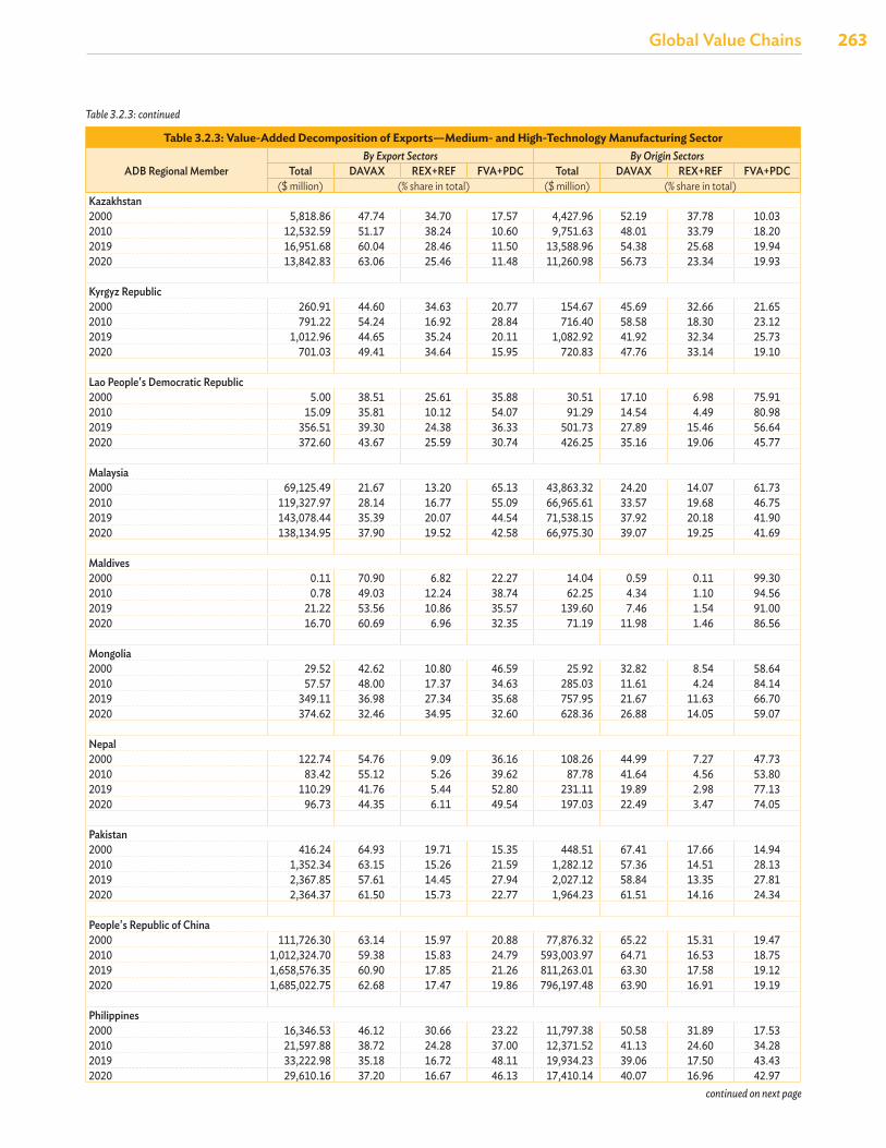
Global Value Chains
263Global Value Chains
Table 3.2.3: Value-Added Decomposition of Exports—Medium- and High-Technology Manufacturing Sector
ADB Regional MemberBy Export Sectors By Origin Sectors
Total DAVAX REX+REF FVA+PDC Total DAVAX REX+REF FVA+PDC($ million) (% share in total) ($ million) (% share in total)
Kazakhstan2000 5,818.86 47.74 34.70 17.57 4,427.96 52.19 37.78 10.032010 12,532.59 51.17 38.24 10.60 9,751.63 48.01 33.79 18.202019 16,951.68 60.04 28.46 11.50 13,588.96 54.38 25.68 19.942020 13,842.83 63.06 25.46 11.48 11,260.98 56.73 23.34 19.93
Kyrgyz Republic2000 260.91 44.60 34.63 20.77 154.67 45.69 32.66 21.652010 791.22 54.24 16.92 28.84 716.40 58.58 18.30 23.122019 1,012.96 44.65 35.24 20.11 1,082.92 41.92 32.34 25.732020 701.03 49.41 34.64 15.95 720.83 47.76 33.14 19.10
Lao People's Democratic Republic2000 5.00 38.51 25.61 35.88 30.51 17.10 6.98 75.912010 15.09 35.81 10.12 54.07 91.29 14.54 4.49 80.982019 356.51 39.30 24.38 36.33 501.73 27.89 15.46 56.642020 372.60 43.67 25.59 30.74 426.25 35.16 19.06 45.77
Malaysia2000 69,125.49 21.67 13.20 65.13 43,863.32 24.20 14.07 61.732010 119,327.97 28.14 16.77 55.09 66,965.61 33.57 19.68 46.752019 143,078.44 35.39 20.07 44.54 71,538.15 37.92 20.18 41.902020 138,134.95 37.90 19.52 42.58 66,975.30 39.07 19.25 41.69
Maldives2000 0.11 70.90 6.82 22.27 14.04 0.59 0.11 99.302010 0.78 49.03 12.24 38.74 62.25 4.34 1.10 94.562019 21.22 53.56 10.86 35.57 139.60 7.46 1.54 91.002020 16.70 60.69 6.96 32.35 71.19 11.98 1.46 86.56
Mongolia2000 29.52 42.62 10.80 46.59 25.92 32.82 8.54 58.642010 57.57 48.00 17.37 34.63 285.03 11.61 4.24 84.142019 349.11 36.98 27.34 35.68 757.95 21.67 11.63 66.702020 374.62 32.46 34.95 32.60 628.36 26.88 14.05 59.07
Nepal2000 122.74 54.76 9.09 36.16 108.26 44.99 7.27 47.732010 83.42 55.12 5.26 39.62 87.78 41.64 4.56 53.802019 110.29 41.76 5.44 52.80 231.11 19.89 2.98 77.132020 96.73 44.35 6.11 49.54 197.03 22.49 3.47 74.05
Pakistan2000 416.24 64.93 19.71 15.35 448.51 67.41 17.66 14.942010 1,352.34 63.15 15.26 21.59 1,282.12 57.36 14.51 28.132019 2,367.85 57.61 14.45 27.94 2,027.12 58.84 13.35 27.812020 2,364.37 61.50 15.73 22.77 1,964.23 61.51 14.16 24.34
People's Republic of China2000 111,726.30 63.14 15.97 20.88 77,876.32 65.22 15.31 19.472010 1,012,324.70 59.38 15.83 24.79 593,003.97 64.71 16.53 18.752019 1,658,576.35 60.90 17.85 21.26 811,263.01 63.30 17.58 19.122020 1,685,022.75 62.68 17.47 19.86 796,197.48 63.90 16.91 19.19
Philippines2000 16,346.53 46.12 30.66 23.22 11,797.38 50.58 31.89 17.532010 21,597.88 38.72 24.28 37.00 12,371.52 41.13 24.60 34.282019 33,222.98 35.18 16.72 48.11 19,934.23 39.06 17.50 43.432020 29,610.16 37.20 16.67 46.13 17,410.14 40.07 16.96 42.97
Table 3.2.3: continued
continued on next page
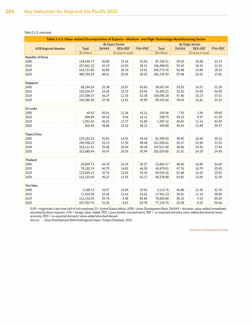
264 Key Indicators for Asia and the Pacific 2021
Table 3.2.3: Value-Added Decomposition of Exports—Medium- and High-Technology Manufacturing Sector
ADB Regional MemberBy Export Sectors By Origin Sectors
Total DAVAX REX+REF FVA+PDC Total DAVAX REX+REF FVA+PDC($ million) (% share in total) ($ million) (% share in total)
Republic of Korea2000 134,640.73 50.80 15.63 33.56 87,358.31 59.50 18.38 22.132010 427,862.23 47.19 14.50 38.31 246,488.91 59.43 18.42 22.152019 516,721.85 46.80 20.19 33.01 300,773.76 56.88 24.80 18.322020 480,794.35 48.91 20.55 30.55 281,139.30 57.68 24.52 17.81
Singapore2000 68,194.56 25.38 10.97 63.65 39,007.84 33.93 14.57 51.502010 139,236.37 24.26 10.19 65.55 76,495.21 35.32 14.59 50.092019 225,308.17 36.27 11.35 52.38 100,040.28 47.46 15.23 37.312020 196,386.36 37.48 12.61 49.90 90,425.66 49.04 16.81 34.15
Sri Lanka2000 40.62 45.61 11.26 43.13 245.46 7.50 1.90 90.602010 898.89 49.33 9.56 41.11 938.75 49.24 9.37 41.392019 1,051.63 46.53 11.77 41.69 1,307.16 46.82 11.14 42.042020 818.46 48.86 13.02 38.12 939.80 48.54 11.89 39.57
Taipei,China2000 119,181.53 41.81 14.01 44.18 81,390.00 48.45 16.40 35.162010 240,938.23 34.13 17.39 48.48 151,056.61 45.17 23.30 31.532019 310,111.41 39.68 20.04 40.28 197,017.66 48.06 24.30 27.642020 313,680.94 43.47 20.59 35.94 201,029.85 51.31 24.29 24.40
Thailand2000 20,839.73 44.29 16.34 39.37 13,864.17 48.46 16.89 34.652010 79,185.74 40.79 14.82 44.39 43,479.01 47.76 16.79 35.452019 123,830.13 42.76 13.04 44.20 69,554.26 51.88 14.20 33.922020 112,133.00 45.27 12.55 42.17 60,578.88 54.82 13.69 31.49
Viet Nam2000 2,188.72 54.57 15.80 29.63 3,115.76 46.88 11.36 41.762010 17,018.58 33.36 13.62 53.02 17,501.23 30.01 11.10 58.892019 111,142.03 29.76 9.38 60.86 78,828.86 30.15 9.16 60.692020 107,555.70 31.55 8.67 59.78 77,134.70 32.08 8.25 59.66
0.00 = magnitude is less than half of unit employed, $ = United States dollars, ADB = Asian Development Bank, DAVAX = domestic value-added immediately absorbed by direct importer, FVA = foreign value-added, PDC = pure double-counted terms, REF = re-exported domestic value-added absorbed by home economy, REX = re-exported domestic value-added absorbed abroad.Source: Asian Development Bank Multiregional Input–Output Database, 2021.
Table 3.2.3: continued
Click here to download the table
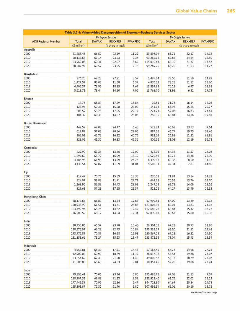
Global Value Chains
265Global Value Chains
Table 3.2.4: Value-Added Decomposition of Exports—Business Services Sector
ADB Regional MemberBy Export Sectors By Origin Sectors
Total DAVAX REX+REF FVA+PDC Total DAVAX REX+REF FVA+PDC($ million) (% share in total) ($ million) (% share in total)
Australia2000 21,285.45 66.52 22.19 11.29 33,898.04 63.71 22.17 14.122010 50,135.67 67.14 23.53 9.34 93,265.12 62.86 24.64 12.502019 53,969.08 69.31 22.07 8.62 115,010.64 65.10 21.37 13.532020 38,287.97 69.57 23.25 7.18 99,269.25 66.70 21.53 11.77
Bangladesh2000 376.20 69.23 27.21 3.57 1,497.04 73.56 11.50 14.932010 1,427.57 83.03 11.58 5.39 4,870.33 73.28 11.12 15.602019 4,406.37 73.96 18.35 7.69 13,554.95 70.15 6.47 23.382020 5,613.71 78.44 14.50 7.06 13,765.70 73.95 6.32 19.73
Bhutan2000 17.78 68.87 17.29 13.84 19.51 71.78 16.14 12.082010 123.96 59.38 15.58 25.05 141.03 63.98 15.25 20.772019 203.59 53.78 17.05 29.17 274.21 59.06 16.33 24.612020 184.39 60.38 14.57 25.06 250.35 65.84 14.36 19.81
Brunei Darussalam2000 442.57 69.08 24.47 6.45 522.24 66.63 23.73 9.642010 612.82 57.08 20.86 22.06 887.36 46.79 19.75 33.462019 502.01 42.72 16.52 40.76 932.03 26.98 11.21 61.812020 323.02 41.32 16.33 42.36 806.12 31.03 12.19 56.78
Cambodia2000 429.90 67.33 13.66 19.00 472.05 64.36 11.57 24.082010 1,597.60 65.72 16.09 18.19 1,525.56 62.72 14.38 22.902019 4,486.93 61.95 13.29 24.76 6,390.98 60.38 8.50 31.132020 3,133.54 57.07 11.09 31.84 5,502.31 47.34 7.81 44.85
Fiji2000 119.47 70.76 15.89 13.35 270.51 71.94 13.84 14.222010 824.07 58.88 11.41 29.71 662.28 70.55 13.76 15.702019 1,168.90 56.59 14.43 28.98 1,249.23 62.75 14.09 23.162020 329.68 57.28 17.15 25.57 518.22 64.17 13.49 22.33
Hong Kong, China2000 68,177.65 66.80 13.54 19.66 67,999.51 67.00 13.89 19.122010 120,938.90 61.51 13.61 24.88 123,002.96 62.01 13.83 24.162019 104,499.94 65.76 14.82 19.42 117,685.28 65.84 15.42 18.732020 76,205.59 68.12 14.54 17.34 92,090.03 68.67 15.00 16.32
India2000 18,750.86 65.57 23.98 10.45 26,304.38 67.21 20.93 11.862010 128,576.97 66.23 22.93 10.84 155,335.29 65.50 21.82 12.682019 193,972.89 70.89 16.18 12.93 250,867.28 69.28 16.22 14.502020 181,358.66 73.27 15.23 11.49 233,872.35 71.04 15.43 13.54
Indonesia2000 4,957.81 68.37 17.21 14.43 17,168.40 57.78 14.98 27.242010 12,909.05 69.99 18.89 11.12 38,017.38 57.54 19.38 23.072019 23,554.62 67.40 21.20 11.40 49,005.57 58.13 18.79 23.072020 11,586.88 65.63 24.53 9.84 38,351.45 57.20 19.06 23.74
Japan2000 99,395.41 70.06 23.14 6.80 195,495.78 69.08 21.83 9.092010 188,197.35 69.88 21.53 8.59 333,922.40 65.76 22.02 12.222019 177,441.39 70.96 22.56 6.47 344,725.30 64.69 20.54 14.782020 155,308.87 72.30 21.90 5.80 307,695.54 66.06 20.19 13.75
continued on next page
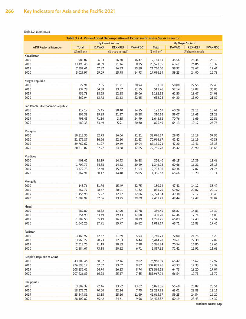
266 Key Indicators for Asia and the Pacific 2021
Table 3.2.4: Value-Added Decomposition of Exports—Business Services Sector
ADB Regional MemberBy Export Sectors By Origin Sectors
Total DAVAX REX+REF FVA+PDC Total DAVAX REX+REF FVA+PDC($ million) (% share in total) ($ million) (% share in total)
Kazakhstan2000 980.87 56.83 26.70 16.47 2,164.81 45.56 26.34 28.102010 13,190.45 70.59 21.16 8.25 20,571.55 63.61 26.06 10.322019 7,597.41 67.87 16.33 15.80 21,750.00 58.92 23.67 17.412020 5,029.97 69.09 15.98 14.93 17,096.54 59.23 24.00 16.78
Kyrgyz Republic2000 22.91 57.35 21.71 20.94 93.00 50.00 22.55 27.452010 239.78 54.88 13.57 31.55 511.46 52.14 12.02 35.852019 956.73 58.65 12.28 29.06 1,132.53 62.50 13.47 24.032020 362.94 63.72 13.63 22.65 633.23 64.30 13.90 21.80
Lao People's Democratic Republic2000 117.17 55.45 20.40 24.15 122.67 60.28 21.11 18.612010 192.38 59.35 21.37 19.28 310.56 59.07 19.65 21.282019 993.45 71.16 3.85 24.99 1,648.32 70.76 6.69 22.562020 480.33 73.49 5.91 20.60 875.49 64.13 10.12 25.75
Malaysia2000 10,818.36 52.73 16.06 31.21 32,096.27 29.85 12.19 57.962010 31,179.87 56.26 22.10 21.63 70,966.67 41.42 16.19 42.382019 39,762.62 61.27 19.69 19.04 87,155.21 47.20 19.41 33.382020 20,610.07 57.97 24.38 17.65 72,755.78 45.42 20.90 33.68
Maldives2000 408.42 58.39 14.93 26.68 326.40 69.15 17.39 13.462010 1,707.77 54.88 14.63 30.49 1,346.78 60.66 16.21 23.132019 3,472.73 52.60 15.87 31.54 2,703.06 60.36 17.87 21.762020 1,762.91 60.47 14.48 25.05 1,356.67 65.66 15.20 19.14
Mongolia2000 145.76 51.76 15.49 32.75 180.94 47.41 14.12 38.472010 667.77 58.67 20.01 21.32 884.70 59.02 20.82 20.172019 1,156.98 55.22 12.72 32.06 2,774.84 49.38 12.17 38.452020 1,009.92 57.06 13.25 29.69 2,401.71 49.44 12.49 38.07
Nepal2000 289.89 68.32 17.90 13.78 389.45 68.87 14.83 16.302010 354.90 63.49 19.43 17.08 430.20 67.46 17.74 14.802019 1,309.53 55.49 16.22 28.29 1,298.75 65.03 17.43 17.542020 1,046.26 57.91 15.97 26.12 1,015.17 65.71 16.83 17.46
Pakistan2000 3,163.92 72.67 21.39 5.94 3,740.71 72.00 21.75 6.252010 3,963.22 70.73 22.83 6.44 6,444.28 70.61 22.30 7.092019 2,618.76 71.19 20.83 7.98 6,396.84 70.54 16.80 12.662020 2,184.67 73.18 20.12 6.71 5,817.32 72.41 15.91 11.68
People's Republic of China2000 43,309.46 68.02 22.16 9.82 76,968.89 65.42 16.62 17.972010 276,698.17 67.07 23.07 9.87 534,089.96 63.33 17.33 19.342019 208,236.42 64.74 26.53 8.74 873,596.18 64.73 18.20 17.072020 207,926.89 66.98 25.17 7.85 885,967.74 66.54 17.73 15.72
Philippines2000 3,802.32 72.46 13.92 13.62 6,821.05 55.60 20.89 23.512010 18,372.71 70.00 22.24 7.75 23,259.95 63.01 23.88 13.112019 35,847.81 63.15 25.16 11.69 41,065.97 59.25 24.54 16.202020 28,102.82 65.42 24.61 9.98 34,478.87 60.19 23.43 16.37
continued on next page
Table 3.2.4: continued
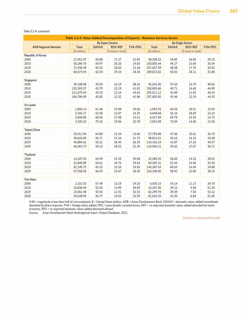
Global Value Chains
267Global Value Chains
Table 3.2.4: Value-Added Decomposition of Exports—Business Services Sector
ADB Regional MemberBy Export Sectors By Origin Sectors
Total DAVAX REX+REF FVA+PDC Total DAVAX REX+REF FVA+PDC($ million) (% share in total) ($ million) (% share in total)
Republic of Korea2000 21,951.07 69.88 17.27 12.85 58,358.15 54.85 16.00 29.152010 50,284.70 59.97 20.20 19.83 150,005.44 49.27 15.69 35.042019 72,438.39 60.32 18.50 21.18 207,657.59 48.38 17.70 33.922020 60,673.94 62.54 19.10 18.36 189,813.02 50.02 18.11 31.86
Singapore2000 39,108.58 45.50 16.19 38.32 55,615.30 37.63 13.75 48.622010 135,393.07 43.79 15.19 41.02 158,805.66 40.71 14.40 44.892019 211,675.54 43.23 12.14 44.63 295,011.12 41.89 11.92 46.192020 184,786.09 45.82 12.32 41.86 257,835.85 43.46 12.19 44.35
Sri Lanka2000 1,856.14 61.36 19.58 19.06 1,954.76 64.56 19.51 15.932010 3,182.17 63.58 22.07 14.35 4,048.68 65.16 18.69 16.152019 5,846.80 68.50 17.98 13.51 6,417.84 69.78 15.50 14.722020 2,925.22 70.16 19.06 10.78 3,823.08 72.04 14.40 13.56
Taipei,China2000 25,911.94 64.80 21.54 13.66 57,793.88 47.66 15.61 36.732010 49,626.00 56.71 21.54 21.75 98,814.21 40.16 16.16 43.682019 45,884.61 55.21 18.40 26.39 119,416.24 41.87 17.16 40.972020 46,063.73 59.13 18.52 22.35 119,569.21 45.62 17.67 36.71
Thailand2000 14,187.30 64.99 15.33 19.68 23,289.25 56.83 14.25 28.922010 31,849.89 63.61 16.76 19.63 60,392.31 52.44 15.06 32.502019 92,140.75 65.32 15.26 19.42 144,287.63 60.63 14.49 24.882020 37,558.58 66.03 15.67 18.30 103,438.00 58.92 12.85 28.23
Viet Nam2000 2,315.33 67.49 13.19 19.33 4,505.15 54.14 11.17 34.702010 10,830.04 55.92 13.99 30.09 24,297.05 39.12 9.58 51.302019 23,061.48 55.56 11.92 32.53 82,299.78 39.39 7.50 53.122020 20,638.59 56.77 10.63 32.59 81,619.20 41.50 6.84 51.65
0.00 = magnitude is less than half of unit employed, $ = United States dollars, ADB = Asian Development Bank, DAVAX = domestic value-added immediately absorbed by direct importer, FVA = foreign value-added, PDC = pure double-counted terms, REF = re-exported domestic value-added absorbed by home economy, REX = re-exported domestic value-added absorbed abroad.Source: Asian Development Bank Multiregional Input–Output Database, 2021.
Table 3.2.4: continued
Click here to download the table
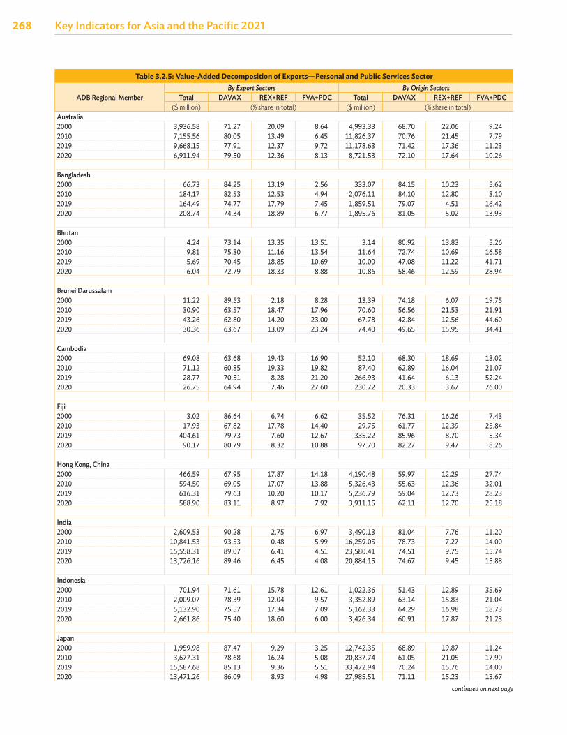
268 Key Indicators for Asia and the Pacific 2021
Table 3.2.5: Value-Added Decomposition of Exports—Personal and Public Services Sector
ADB Regional MemberBy Export Sectors By Origin Sectors
Total DAVAX REX+REF FVA+PDC Total DAVAX REX+REF FVA+PDC($ million) (% share in total) ($ million) (% share in total)
Australia2000 3,936.58 71.27 20.09 8.64 4,993.33 68.70 22.06 9.242010 7,155.56 80.05 13.49 6.45 11,826.37 70.76 21.45 7.792019 9,668.15 77.91 12.37 9.72 11,178.63 71.42 17.36 11.232020 6,911.94 79.50 12.36 8.13 8,721.53 72.10 17.64 10.26
Bangladesh2000 66.73 84.25 13.19 2.56 333.07 84.15 10.23 5.622010 184.17 82.53 12.53 4.94 2,076.11 84.10 12.80 3.102019 164.49 74.77 17.79 7.45 1,859.51 79.07 4.51 16.422020 208.74 74.34 18.89 6.77 1,895.76 81.05 5.02 13.93
Bhutan2000 4.24 73.14 13.35 13.51 3.14 80.92 13.83 5.262010 9.81 75.30 11.16 13.54 11.64 72.74 10.69 16.582019 5.69 70.45 18.85 10.69 10.00 47.08 11.22 41.712020 6.04 72.79 18.33 8.88 10.86 58.46 12.59 28.94
Brunei Darussalam2000 11.22 89.53 2.18 8.28 13.39 74.18 6.07 19.752010 30.90 63.57 18.47 17.96 70.60 56.56 21.53 21.912019 43.26 62.80 14.20 23.00 67.78 42.84 12.56 44.602020 30.36 63.67 13.09 23.24 74.40 49.65 15.95 34.41
Cambodia2000 69.08 63.68 19.43 16.90 52.10 68.30 18.69 13.022010 71.12 60.85 19.33 19.82 87.40 62.89 16.04 21.072019 28.77 70.51 8.28 21.20 266.93 41.64 6.13 52.242020 26.75 64.94 7.46 27.60 230.72 20.33 3.67 76.00
Fiji2000 3.02 86.64 6.74 6.62 35.52 76.31 16.26 7.432010 17.93 67.82 17.78 14.40 29.75 61.77 12.39 25.842019 404.61 79.73 7.60 12.67 335.22 85.96 8.70 5.342020 90.17 80.79 8.32 10.88 97.70 82.27 9.47 8.26
Hong Kong, China2000 466.59 67.95 17.87 14.18 4,190.48 59.97 12.29 27.742010 594.50 69.05 17.07 13.88 5,326.43 55.63 12.36 32.012019 616.31 79.63 10.20 10.17 5,236.79 59.04 12.73 28.232020 588.90 83.11 8.97 7.92 3,911.15 62.11 12.70 25.18
India2000 2,609.53 90.28 2.75 6.97 3,490.13 81.04 7.76 11.202010 10,841.53 93.53 0.48 5.99 16,259.05 78.73 7.27 14.002019 15,558.31 89.07 6.41 4.51 23,580.41 74.51 9.75 15.742020 13,726.16 89.46 6.45 4.08 20,884.15 74.67 9.45 15.88
Indonesia2000 701.94 71.61 15.78 12.61 1,022.36 51.43 12.89 35.692010 2,009.07 78.39 12.04 9.57 3,352.89 63.14 15.83 21.042019 5,132.90 75.57 17.34 7.09 5,162.33 64.29 16.98 18.732020 2,661.86 75.40 18.60 6.00 3,426.34 60.91 17.87 21.23
Japan2000 1,959.98 87.47 9.29 3.25 12,742.35 68.89 19.87 11.242010 3,677.31 78.68 16.24 5.08 20,837.74 61.05 21.05 17.902019 15,587.68 85.13 9.36 5.51 33,472.94 70.24 15.76 14.002020 13,471.26 86.09 8.93 4.98 27,985.51 71.11 15.23 13.67
continued on next page
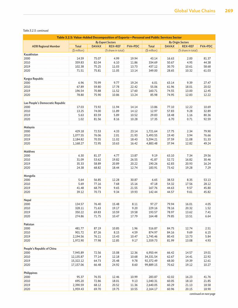
Global Value Chains
269Global Value Chains
Table 3.2.5: Value-Added Decomposition of Exports—Personal and Public Services Sector
ADB Regional MemberBy Export Sectors By Origin Sectors
Total DAVAX REX+REF FVA+PDC Total DAVAX REX+REF FVA+PDC($ million) (% share in total) ($ million) (% share in total)
Kazakhstan2000 14.59 75.07 4.99 19.94 43.14 16.63 2.00 81.372010 359.83 82.04 6.10 11.86 334.69 50.67 4.95 44.382019 102.38 75.25 11.03 13.73 437.12 30.70 10.61 58.682020 71.51 75.81 11.05 13.14 349.00 28.65 10.32 61.03
Kyrgyz Republic2000 6.96 70.99 9.77 19.24 6.01 63.14 9.39 27.472010 67.89 59.80 17.78 22.42 55.06 61.96 18.01 20.022019 196.54 70.88 11.52 17.60 160.71 74.55 13.00 12.452020 78.80 75.90 10.86 13.24 85.98 74.95 12.83 12.22
Lao People's Democratic Republic2000 17.03 73.92 11.94 14.14 13.86 77.10 12.22 10.692010 13.25 74.00 11.89 14.12 12.97 57.83 9.28 32.892019 5.63 83.59 5.89 10.52 29.83 18.48 1.16 80.362020 1.02 81.56 8.16 10.28 17.35 6.70 0.71 92.59
Malaysia2000 429.18 72.53 4.33 23.14 1,721.64 17.75 2.34 79.902010 1,077.55 76.06 2.01 21.93 5,493.55 19.40 3.94 76.662019 2,184.82 70.55 11.02 18.43 5,594.21 37.59 11.08 51.332020 1,168.27 72.95 10.63 16.42 4,883.48 37.94 12.82 49.24
Maldives2000 6.30 81.37 4.77 13.87 9.19 63.10 7.34 29.562010 31.09 53.62 19.82 26.55 41.87 52.72 16.82 30.462019 35.33 58.89 20.89 20.22 190.26 62.83 20.93 16.242020 24.38 68.82 18.44 12.74 183.91 73.42 19.28 7.29
Mongolia2000 5.64 56.85 12.28 30.87 6.65 38.53 8.35 53.132010 5.69 77.16 7.68 15.16 47.18 54.32 17.56 28.122019 41.48 68.79 9.65 21.55 167.76 44.63 9.57 45.802020 39.12 70.73 9.34 19.93 142.44 44.57 9.61 45.82
Nepal2000 134.57 76.40 15.48 8.11 97.27 79.94 16.01 4.052010 328.11 71.63 19.17 9.20 229.16 78.16 20.32 1.522019 350.22 69.83 10.59 19.58 193.57 78.97 13.62 7.412020 274.86 71.75 10.47 17.79 164.48 79.85 13.51 6.64
Pakistan2000 481.77 87.19 10.85 1.96 516.87 84.75 12.74 2.512010 901.72 87.26 8.15 4.59 874.97 84.16 9.69 6.152019 2,194.56 76.11 13.43 10.47 1,745.46 80.43 13.73 5.842020 1,972.90 77.98 12.85 9.17 1,559.73 81.99 13.08 4.93
People's Republic of China2000 7,945.89 72.56 15.08 12.36 6,950.44 66.42 14.57 19.012010 12,135.87 77.14 12.18 10.68 34,331.54 62.67 14.41 22.922019 15,322.12 64.73 25.48 9.78 92,372.49 68.00 19.39 12.612020 17,157.06 66.48 24.92 8.60 99,889.15 70.62 19.12 10.27
Philippines2000 95.37 76.55 12.46 10.99 283.87 42.02 16.23 41.762010 695.20 72.86 18.01 9.13 1,040.31 60.05 18.10 21.852019 2,390.59 68.12 20.52 11.36 2,640.05 60.29 21.13 18.582020 1,959.43 69.70 19.75 10.55 2,164.17 60.96 20.15 18.90
Table 3.2.5: continued
continued on next page
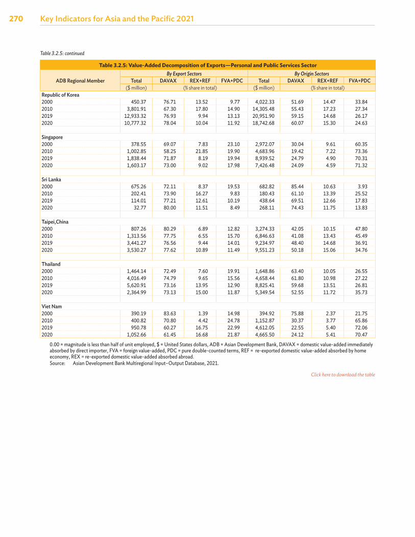
270 Key Indicators for Asia and the Pacific 2021
Table 3.2.5: Value-Added Decomposition of Exports—Personal and Public Services Sector
ADB Regional MemberBy Export Sectors By Origin Sectors
Total DAVAX REX+REF FVA+PDC Total DAVAX REX+REF FVA+PDC($ million) (% share in total) ($ million) (% share in total)
Republic of Korea2000 450.37 76.71 13.52 9.77 4,022.33 51.69 14.47 33.842010 3,801.91 67.30 17.80 14.90 14,305.48 55.43 17.23 27.342019 12,933.32 76.93 9.94 13.13 20,951.90 59.15 14.68 26.172020 10,777.32 78.04 10.04 11.92 18,742.68 60.07 15.30 24.63
Singapore2000 378.55 69.07 7.83 23.10 2,972.07 30.04 9.61 60.352010 1,002.85 58.25 21.85 19.90 4,683.96 19.42 7.22 73.362019 1,838.44 71.87 8.19 19.94 8,939.52 24.79 4.90 70.312020 1,603.17 73.00 9.02 17.98 7,426.48 24.09 4.59 71.32
Sri Lanka2000 675.26 72.11 8.37 19.53 682.82 85.44 10.63 3.932010 202.41 73.90 16.27 9.83 180.43 61.10 13.39 25.522019 114.01 77.21 12.61 10.19 438.64 69.51 12.66 17.832020 32.77 80.00 11.51 8.49 268.11 74.43 11.75 13.83
Taipei,China2000 807.26 80.29 6.89 12.82 3,274.33 42.05 10.15 47.802010 1,313.56 77.75 6.55 15.70 6,846.63 41.08 13.43 45.492019 3,441.27 76.56 9.44 14.01 9,234.97 48.40 14.68 36.912020 3,530.27 77.62 10.89 11.49 9,551.23 50.18 15.06 34.76
Thailand2000 1,464.14 72.49 7.60 19.91 1,648.86 63.40 10.05 26.552010 4,016.49 74.79 9.65 15.56 4,658.44 61.80 10.98 27.222019 5,620.91 73.16 13.95 12.90 8,825.41 59.68 13.51 26.812020 2,364.99 73.13 15.00 11.87 5,349.54 52.55 11.72 35.73
Viet Nam2000 390.19 83.63 1.39 14.98 394.92 75.88 2.37 21.752010 400.82 70.80 4.42 24.78 1,152.87 30.37 3.77 65.862019 950.78 60.27 16.75 22.99 4,612.05 22.55 5.40 72.062020 1,052.66 61.45 16.68 21.87 4,665.50 24.12 5.41 70.47
0.00 = magnitude is less than half of unit employed, $ = United States dollars, ADB = Asian Development Bank, DAVAX = domestic value-added immediately absorbed by direct importer, FVA = foreign value-added, PDC = pure double-counted terms, REF = re-exported domestic value-added absorbed by home economy, REX = re-exported domestic value-added absorbed abroad.Source: Asian Development Bank Multiregional Input–Output Database, 2021.
Table 3.2.5: continued
Click here to download the table
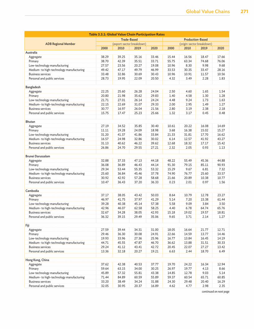
Global Value Chains
271Global Value Chains
Table 3.3.1: Global Value Chain Participation Rates
ADB Regional MemberTrade-Based Production-Based
(export-sector breakdown) (origin-sector breakdown)2000 2010 2019 2020 2000 2010 2019 2020
AustraliaAggregate 38.29 39.25 35.16 33.46 15.44 16.56 18.47 17.66Primary 38.70 42.39 35.51 33.71 55.75 63.34 74.68 76.06Low-technology manufacturing 27.57 23.56 20.27 19.08 10.96 8.30 9.98 9.68Medium- to high-technology manufacturing 49.42 47.17 49.79 46.99 33.53 30.35 33.47 28.16Business services 33.48 32.86 30.69 30.43 10.96 10.91 11.57 10.56Personal and public services 28.73 19.95 22.09 20.50 4.32 3.49 2.28 1.83
BangladeshAggregate 22.25 25.60 26.28 24.04 2.50 4.60 1.65 1.54Primary 20.80 21.98 35.62 29.83 1.40 4.58 1.30 1.28Low-technology manufacturing 21.71 27.01 26.14 24.24 4.48 9.24 1.73 1.63Medium- to high-technology manufacturing 22.15 22.69 31.07 29.33 2.00 2.95 1.49 1.27Business services 30.77 16.97 26.04 21.56 2.80 3.19 2.38 2.18Personal and public services 15.75 17.47 25.23 25.66 1.32 3.17 0.45 0.48
BhutanAggregate 27.19 34.52 35.85 30.40 10.61 20.22 16.08 14.69Primary 11.11 19.28 24.09 18.98 3.68 16.38 15.02 15.27Low-technology manufacturing 31.20 41.37 41.86 33.84 21.33 31.81 17.70 16.62Medium- to high-technology manufacturing 16.57 24.98 32.86 30.02 6.14 12.57 41.92 43.27Business services 31.13 40.62 46.22 39.62 12.68 18.32 17.17 15.42Personal and public services 26.86 24.70 29.55 27.21 2.32 2.05 0.93 1.13
Brunei DarussalamAggregate 32.88 37.33 47.13 44.18 48.22 55.49 45.36 44.88Primary 36.08 36.89 46.43 44.14 91.30 79.15 85.11 90.93Low-technology manufacturing 29.34 53.44 55.35 53.32 15.29 9.67 6.81 7.32Medium- to high-technology manufacturing 25.60 36.84 45.46 37.78 74.90 76.77 25.60 33.57Business services 30.92 42.92 57.28 58.68 21.66 20.89 10.38 10.77Personal and public services 10.47 36.43 37.20 36.33 0.23 2.01 0.97 1.56
CambodiaAggregate 37.17 38.05 43.42 50.03 8.64 10.79 12.78 23.27Primary 46.97 41.75 37.97 41.29 5.14 7.20 15.38 61.44Low-technology manufacturing 39.28 40.38 45.14 57.38 5.58 9.09 3.84 3.50Medium- to high-technology manufacturing 42.96 46.07 62.58 58.25 4.40 6.78 64.74 65.76Business services 32.67 34.28 38.05 42.93 15.18 19.02 19.57 18.81Personal and public services 36.32 39.15 29.49 35.06 9.65 3.71 2.14 1.27
FijiAggregate 27.59 39.44 34.31 31.00 18.05 16.64 21.77 12.71Primary 29.46 36.30 30.08 24.91 22.66 14.59 13.77 14.46Low-technology manufacturing 19.93 33.96 27.36 25.96 16.77 13.84 16.45 14.19Medium- to high-technology manufacturing 44.71 45.55 47.87 46.70 36.62 13.88 31.51 30.33Business services 29.24 41.12 43.41 42.72 20.45 22.07 27.27 13.42Personal and public services 13.36 32.18 20.27 19.21 6.63 2.44 18.70 6.49
Hong Kong, ChinaAggregate 37.62 42.38 40.53 37.77 19.70 24.22 16.34 12.94Primary 59.64 63.15 34.00 30.25 26.97 19.77 4.13 8.66Low-technology manufacturing 45.89 57.32 55.81 43.38 14.85 12.78 9.03 5.14Medium- to high-technology manufacturing 71.44 84.89 60.59 55.89 59.37 60.54 65.71 60.85Business services 33.20 38.49 34.24 31.88 24.30 29.48 20.40 16.29Personal and public services 32.05 30.95 20.37 16.89 4.62 4.77 2.98 2.35
continued on next page
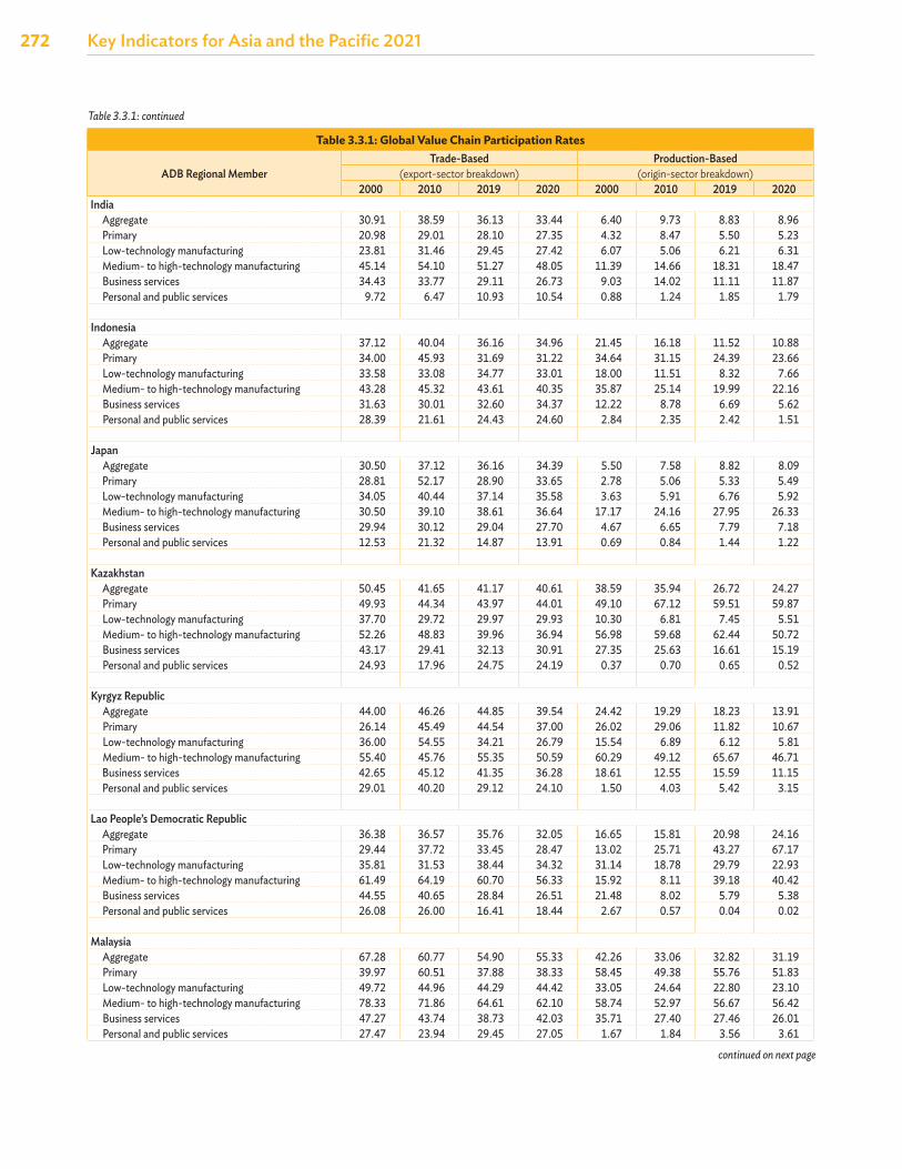
272 Key Indicators for Asia and the Pacific 2021
Table 3.3.1: Global Value Chain Participation Rates
ADB Regional MemberTrade-Based Production-Based
(export-sector breakdown) (origin-sector breakdown)2000 2010 2019 2020 2000 2010 2019 2020
IndiaAggregate 30.91 38.59 36.13 33.44 6.40 9.73 8.83 8.96Primary 20.98 29.01 28.10 27.35 4.32 8.47 5.50 5.23Low-technology manufacturing 23.81 31.46 29.45 27.42 6.07 5.06 6.21 6.31Medium- to high-technology manufacturing 45.14 54.10 51.27 48.05 11.39 14.66 18.31 18.47Business services 34.43 33.77 29.11 26.73 9.03 14.02 11.11 11.87Personal and public services 9.72 6.47 10.93 10.54 0.88 1.24 1.85 1.79
IndonesiaAggregate 37.12 40.04 36.16 34.96 21.45 16.18 11.52 10.88Primary 34.00 45.93 31.69 31.22 34.64 31.15 24.39 23.66Low-technology manufacturing 33.58 33.08 34.77 33.01 18.00 11.51 8.32 7.66Medium- to high-technology manufacturing 43.28 45.32 43.61 40.35 35.87 25.14 19.99 22.16Business services 31.63 30.01 32.60 34.37 12.22 8.78 6.69 5.62Personal and public services 28.39 21.61 24.43 24.60 2.84 2.35 2.42 1.51
JapanAggregate 30.50 37.12 36.16 34.39 5.50 7.58 8.82 8.09Primary 28.81 52.17 28.90 33.65 2.78 5.06 5.33 5.49Low-technology manufacturing 34.05 40.44 37.14 35.58 3.63 5.91 6.76 5.92Medium- to high-technology manufacturing 30.50 39.10 38.61 36.64 17.17 24.16 27.95 26.33Business services 29.94 30.12 29.04 27.70 4.67 6.65 7.79 7.18Personal and public services 12.53 21.32 14.87 13.91 0.69 0.84 1.44 1.22
KazakhstanAggregate 50.45 41.65 41.17 40.61 38.59 35.94 26.72 24.27Primary 49.93 44.34 43.97 44.01 49.10 67.12 59.51 59.87Low-technology manufacturing 37.70 29.72 29.97 29.93 10.30 6.81 7.45 5.51Medium- to high-technology manufacturing 52.26 48.83 39.96 36.94 56.98 59.68 62.44 50.72Business services 43.17 29.41 32.13 30.91 27.35 25.63 16.61 15.19Personal and public services 24.93 17.96 24.75 24.19 0.37 0.70 0.65 0.52
Kyrgyz RepublicAggregate 44.00 46.26 44.85 39.54 24.42 19.29 18.23 13.91Primary 26.14 45.49 44.54 37.00 26.02 29.06 11.82 10.67Low-technology manufacturing 36.00 54.55 34.21 26.79 15.54 6.89 6.12 5.81Medium- to high-technology manufacturing 55.40 45.76 55.35 50.59 60.29 49.12 65.67 46.71Business services 42.65 45.12 41.35 36.28 18.61 12.55 15.59 11.15Personal and public services 29.01 40.20 29.12 24.10 1.50 4.03 5.42 3.15
Lao People’s Democratic RepublicAggregate 36.38 36.57 35.76 32.05 16.65 15.81 20.98 24.16Primary 29.44 37.72 33.45 28.47 13.02 25.71 43.27 67.17Low-technology manufacturing 35.81 31.53 38.44 34.32 31.14 18.78 29.79 22.93Medium- to high-technology manufacturing 61.49 64.19 60.70 56.33 15.92 8.11 39.18 40.42Business services 44.55 40.65 28.84 26.51 21.48 8.02 5.79 5.38Personal and public services 26.08 26.00 16.41 18.44 2.67 0.57 0.04 0.02
MalaysiaAggregate 67.28 60.77 54.90 55.33 42.26 33.06 32.82 31.19Primary 39.97 60.51 37.88 38.33 58.45 49.38 55.76 51.83Low-technology manufacturing 49.72 44.96 44.29 44.42 33.05 24.64 22.80 23.10Medium- to high-technology manufacturing 78.33 71.86 64.61 62.10 58.74 52.97 56.67 56.42Business services 47.27 43.74 38.73 42.03 35.71 27.40 27.46 26.01Personal and public services 27.47 23.94 29.45 27.05 1.67 1.84 3.56 3.61
Table 3.3.1: continued
continued on next page
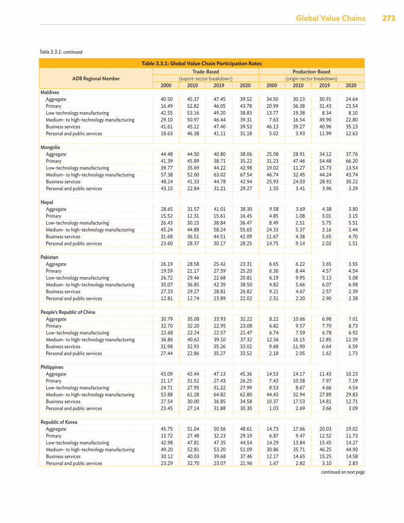
Global Value Chains
273Global Value Chains
Table 3.3.1: Global Value Chain Participation Rates
ADB Regional MemberTrade-Based Production-Based
(export-sector breakdown) (origin-sector breakdown)2000 2010 2019 2020 2000 2010 2019 2020
MaldivesAggregate 40.50 45.37 47.45 39.52 34.50 30.23 30.91 24.64Primary 16.49 52.82 46.05 43.78 20.99 36.38 31.43 23.54Low-technology manufacturing 42.55 53.16 49.20 38.83 13.77 19.38 8.34 8.10Medium- to high-technology manufacturing 29.10 50.97 46.44 39.31 7.63 16.54 49.90 22.80Business services 41.61 45.12 47.40 39.53 46.13 39.27 40.96 35.13Personal and public services 18.63 46.38 41.11 31.18 5.02 3.93 11.99 12.63
MongoliaAggregate 44.48 44.50 40.80 38.06 25.08 28.91 34.12 37.76Primary 41.39 45.89 38.71 35.22 31.23 47.46 54.48 66.20Low-technology manufacturing 39.77 35.69 44.22 42.98 19.02 11.27 15.73 13.54Medium- to high-technology manufacturing 57.38 52.00 63.02 67.54 46.74 32.45 44.24 43.74Business services 48.24 41.33 44.78 42.94 25.93 24.03 28.92 30.22Personal and public services 43.15 22.84 31.21 29.27 1.55 3.41 3.96 3.29
NepalAggregate 28.65 31.57 41.01 38.30 9.58 3.69 4.38 3.80Primary 15.52 12.31 15.61 16.45 4.85 1.08 3.01 3.15Low-technology manufacturing 26.43 30.15 38.84 36.47 8.49 2.51 5.75 5.51Medium- to high-technology manufacturing 45.24 44.88 58.24 55.65 24.33 5.37 3.16 3.44Business services 31.68 36.51 44.51 42.09 11.67 4.38 5.65 4.70Personal and public services 23.60 28.37 30.17 28.25 14.75 9.14 2.02 1.51
PakistanAggregate 26.19 28.58 25.42 23.31 6.65 6.22 3.65 3.55Primary 19.59 21.17 27.59 25.20 6.30 8.44 4.57 4.54Low-technology manufacturing 26.72 29.46 22.68 20.81 6.19 9.95 5.13 5.08Medium- to high-technology manufacturing 35.07 36.85 42.39 38.50 4.82 5.66 6.07 6.98Business services 27.33 29.27 28.81 26.82 9.21 4.67 2.57 2.39Personal and public services 12.81 12.74 23.89 22.02 2.51 2.20 2.90 2.38
People’s Republic of ChinaAggregate 30.79 35.08 33.93 32.22 8.22 10.66 6.98 7.01Primary 32.70 32.20 22.95 23.08 6.82 9.57 7.70 8.73Low-technology manufacturing 22.68 22.24 22.57 21.47 6.74 7.59 6.78 6.92Medium- to high-technology manufacturing 36.86 40.62 39.10 37.32 12.56 16.15 12.85 12.39Business services 31.98 32.93 35.26 33.02 9.68 11.90 6.64 6.59Personal and public services 27.44 22.86 35.27 33.52 2.18 2.05 1.62 1.73
PhilippinesAggregate 43.09 42.44 47.13 45.36 14.53 14.17 11.43 10.23Primary 21.17 31.52 27.43 26.25 7.43 10.58 7.97 7.19Low-technology manufacturing 24.71 27.95 31.22 27.99 8.53 8.67 4.66 4.54Medium- to high-technology manufacturing 53.88 61.28 64.82 62.80 44.43 32.94 27.89 29.83Business services 27.54 30.00 36.85 34.58 10.37 17.53 14.81 12.71Personal and public services 23.45 27.14 31.88 30.30 1.03 2.69 3.66 3.09
Republic of KoreaAggregate 45.75 51.04 50.56 48.61 14.73 17.66 20.03 19.02Primary 15.72 27.48 32.23 29.19 6.87 9.47 12.52 11.73Low-technology manufacturing 42.98 47.81 47.35 44.54 14.29 13.84 15.45 14.27Medium- to high-technology manufacturing 49.20 52.81 53.20 51.09 30.86 35.71 46.25 44.90Business services 30.12 40.03 39.68 37.46 12.17 14.65 15.25 14.58Personal and public services 23.29 32.70 23.07 21.96 1.67 2.82 3.10 2.83
Table 3.3.1: continued
continued on next page
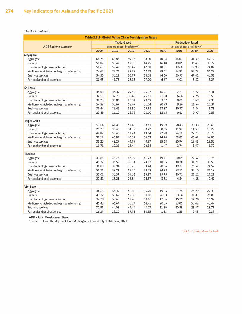
274 Key Indicators for Asia and the Pacific 2021
Table 3.3.1: Global Value Chain Participation Rates
ADB Regional MemberTrade-Based Production-Based
(export-sector breakdown) (origin-sector breakdown)2000 2010 2019 2020 2000 2010 2019 2020
SingaporeAggregate 66.76 65.83 59.93 58.00 40.04 44.07 41.39 42.19Primary 50.89 50.47 63.85 44.45 46.10 40.85 36.45 35.77Low-technology manufacturing 58.65 59.49 50.47 47.58 18.61 19.60 19.93 24.07Medium- to high-technology manufacturing 74.62 75.74 63.73 62.52 58.41 54.93 52.73 56.23Business services 54.50 56.21 56.77 54.18 44.00 50.93 47.42 46.55Personal and public services 30.93 41.75 28.13 27.00 6.67 4.01 3.52 3.27
Sri LankaAggregate 35.05 34.39 29.42 26.17 16.71 7.24 6.72 4.41Primary 34.53 32.76 30.40 25.81 21.30 6.66 7.26 5.58Low-technology manufacturing 36.23 30.86 23.84 20.59 3.57 8.02 5.69 4.30Medium- to high-technology manufacturing 54.39 50.67 53.47 51.14 20.99 9.36 11.54 10.34Business services 38.64 36.42 31.50 29.84 23.87 10.37 9.84 5.75Personal and public services 27.89 26.10 22.79 20.00 12.65 0.63 0.97 0.59
Taipei,ChinaAggregate 53.04 61.46 57.46 53.81 19.99 28.43 30.33 29.69Primary 21.79 35.45 34.39 39.72 8.55 11.97 11.53 10.29Low-technology manufacturing 49.82 58.46 51.74 49.14 22.98 24.19 27.25 25.73Medium- to high-technology manufacturing 58.19 65.87 60.32 56.53 44.28 59.89 66.62 64.05Business services 35.20 43.29 44.79 40.87 15.68 20.94 19.45 19.50Personal and public services 19.71 22.25 23.44 22.38 1.47 2.74 3.67 3.70
ThailandAggregate 43.66 48.73 43.09 41.73 19.71 20.09 22.52 19.76Primary 41.27 36.59 28.84 24.82 18.35 18.28 31.71 38.50Low-technology manufacturing 38.08 39.94 35.70 33.44 20.06 19.23 26.57 24.57Medium- to high-technology manufacturing 55.71 59.21 57.24 54.73 34.78 33.11 32.10 31.19Business services 35.01 36.39 34.68 33.97 19.75 20.71 22.21 17.21Personal and public services 27.51 25.21 26.84 26.87 3.53 4.34 4.88 2.49
Viet NamAggregate 36.65 54.49 58.83 56.70 19.56 21.75 24.79 22.48Primary 41.22 50.62 52.39 50.00 26.83 33.56 31.81 28.89Low-technology manufacturing 34.78 53.69 52.49 50.06 17.86 15.29 17.70 15.92Medium- to high-technology manufacturing 45.43 66.64 70.24 68.45 20.55 33.05 50.42 45.47Business services 32.51 44.08 44.44 43.23 21.39 20.89 25.47 23.71Personal and public services 16.37 29.20 39.73 38.55 1.33 1.55 2.43 2.39
ADB = Asian Development Bank.Source: Asian Development Bank Multiregional Input–Output Database, 2021.
Table 3.3.1: continued
Click here to download the table
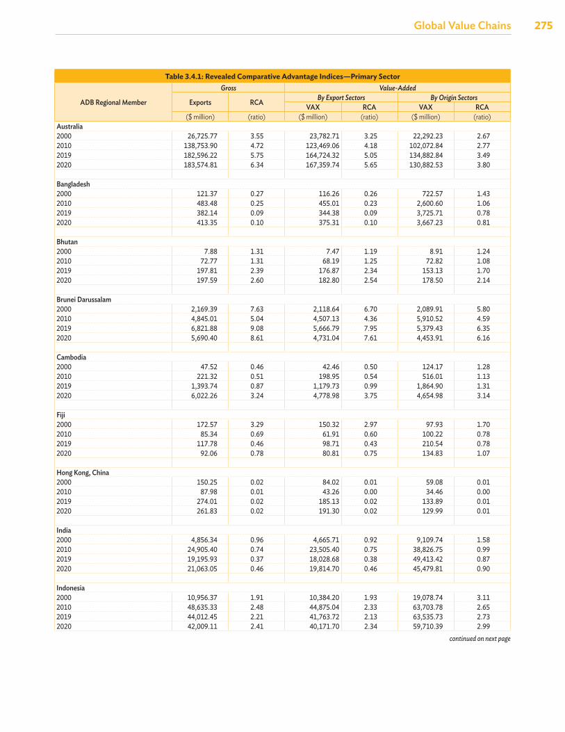
Global Value Chains
275Global Value Chains
Table 3.4.1: Revealed Comparative Advantage Indices—Primary Sector
ADB Regional Member
Gross Value-Added
Exports RCA By Export Sectors By Origin SectorsVAX RCA VAX RCA
($ million) (ratio) ($ million) (ratio) ($ million) (ratio)Australia2000 26,725.77 3.55 23,782.71 3.25 22,292.23 2.67 2010 138,753.90 4.72 123,469.06 4.18 102,072.84 2.77 2019 182,596.22 5.75 164,724.32 5.05 134,882.84 3.49 2020 183,574.81 6.34 167,359.74 5.65 130,882.53 3.80
Bangladesh2000 121.37 0.27 116.26 0.26 722.57 1.43 2010 483.48 0.25 455.01 0.23 2,600.60 1.06 2019 382.14 0.09 344.38 0.09 3,725.71 0.78 2020 413.35 0.10 375.31 0.10 3,667.23 0.81
Bhutan2000 7.88 1.31 7.47 1.19 8.91 1.24 2010 72.77 1.31 68.19 1.25 72.82 1.08 2019 197.81 2.39 176.87 2.34 153.13 1.70 2020 197.59 2.60 182.80 2.54 178.50 2.14
Brunei Darussalam2000 2,169.39 7.63 2,118.64 6.70 2,089.91 5.80 2010 4,845.01 5.04 4,507.13 4.36 5,910.52 4.59 2019 6,821.88 9.08 5,666.79 7.95 5,379.43 6.35 2020 5,690.40 8.61 4,731.04 7.61 4,453.91 6.16
Cambodia2000 47.52 0.46 42.46 0.50 124.17 1.28 2010 221.32 0.51 198.95 0.54 516.01 1.13 2019 1,393.74 0.87 1,179.73 0.99 1,864.90 1.31 2020 6,022.26 3.24 4,778.98 3.75 4,654.98 3.14
Fiji2000 172.57 3.29 150.32 2.97 97.93 1.70 2010 85.34 0.69 61.91 0.60 100.22 0.78 2019 117.78 0.46 98.71 0.43 210.54 0.78 2020 92.06 0.78 80.81 0.75 134.83 1.07
Hong Kong, China2000 150.25 0.02 84.02 0.01 59.08 0.01 2010 87.98 0.01 43.26 0.00 34.46 0.00 2019 274.01 0.02 185.13 0.02 133.89 0.01 2020 261.83 0.02 191.30 0.02 129.99 0.01
India2000 4,856.34 0.96 4,665.71 0.92 9,109.74 1.58 2010 24,905.40 0.74 23,505.40 0.75 38,826.75 0.99 2019 19,195.93 0.37 18,028.68 0.38 49,413.42 0.87 2020 21,063.05 0.46 19,814.70 0.46 45,479.81 0.90
Indonesia2000 10,956.37 1.91 10,384.20 1.93 19,078.74 3.11 2010 48,635.33 2.48 44,875.04 2.33 63,703.78 2.65 2019 44,012.45 2.21 41,763.72 2.13 63,535.73 2.73 2020 42,009.11 2.41 40,171.70 2.34 59,710.39 2.99
continued on next page
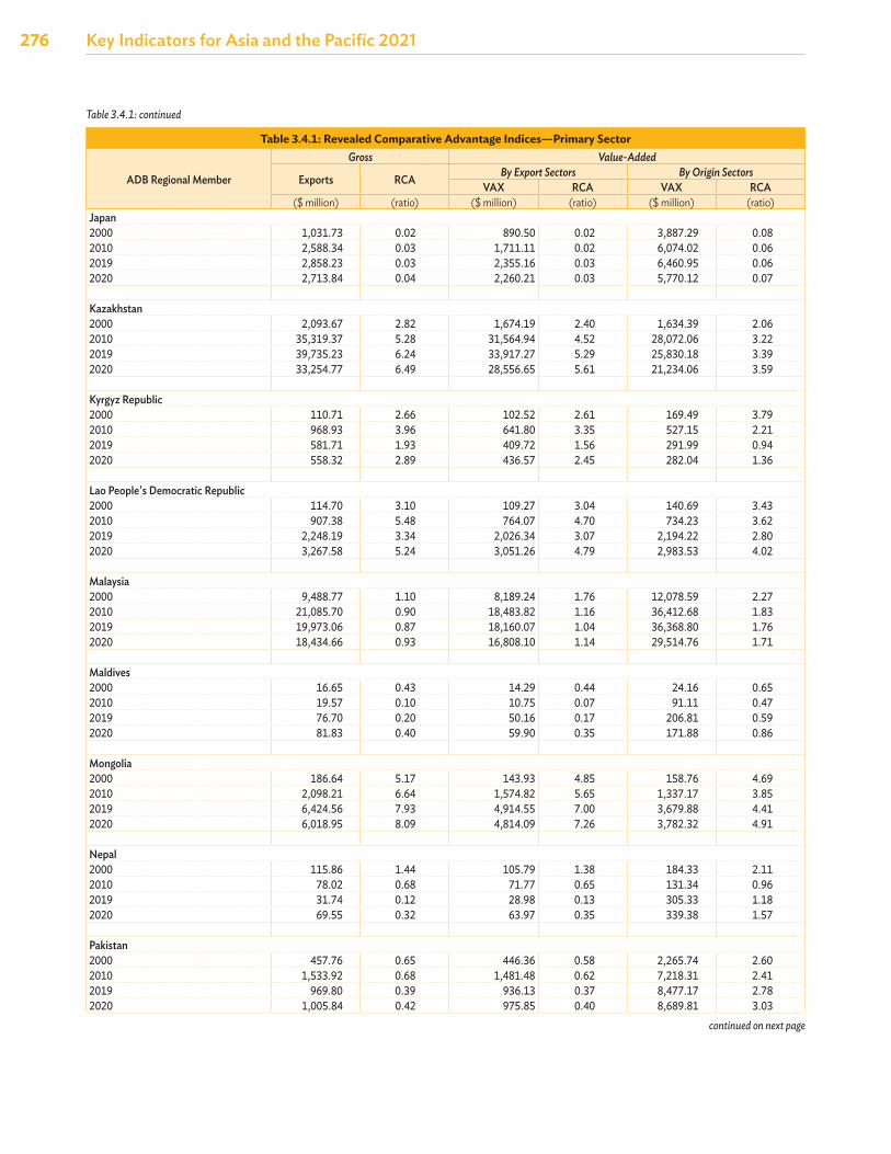
276 Key Indicators for Asia and the Pacific 2021
Table 3.4.1: Revealed Comparative Advantage Indices—Primary Sector
ADB Regional Member
Gross Value-Added
Exports RCA By Export Sectors By Origin SectorsVAX RCA VAX RCA
($ million) (ratio) ($ million) (ratio) ($ million) (ratio)Japan2000 1,031.73 0.02 890.50 0.02 3,887.29 0.08 2010 2,588.34 0.03 1,711.11 0.02 6,074.02 0.06 2019 2,858.23 0.03 2,355.16 0.03 6,460.95 0.06 2020 2,713.84 0.04 2,260.21 0.03 5,770.12 0.07
Kazakhstan2000 2,093.67 2.82 1,674.19 2.40 1,634.39 2.06 2010 35,319.37 5.28 31,564.94 4.52 28,072.06 3.22 2019 39,735.23 6.24 33,917.27 5.29 25,830.18 3.39 2020 33,254.77 6.49 28,556.65 5.61 21,234.06 3.59
Kyrgyz Republic2000 110.71 2.66 102.52 2.61 169.49 3.79 2010 968.93 3.96 641.80 3.35 527.15 2.21 2019 581.71 1.93 409.72 1.56 291.99 0.94 2020 558.32 2.89 436.57 2.45 282.04 1.36
Lao People's Democratic Republic2000 114.70 3.10 109.27 3.04 140.69 3.43 2010 907.38 5.48 764.07 4.70 734.23 3.62 2019 2,248.19 3.34 2,026.34 3.07 2,194.22 2.80 2020 3,267.58 5.24 3,051.26 4.79 2,983.53 4.02
Malaysia2000 9,488.77 1.10 8,189.24 1.76 12,078.59 2.27 2010 21,085.70 0.90 18,483.82 1.16 36,412.68 1.83 2019 19,973.06 0.87 18,160.07 1.04 36,368.80 1.76 2020 18,434.66 0.93 16,808.10 1.14 29,514.76 1.71
Maldives2000 16.65 0.43 14.29 0.44 24.16 0.65 2010 19.57 0.10 10.75 0.07 91.11 0.47 2019 76.70 0.20 50.16 0.17 206.81 0.59 2020 81.83 0.40 59.90 0.35 171.88 0.86
Mongolia2000 186.64 5.17 143.93 4.85 158.76 4.69 2010 2,098.21 6.64 1,574.82 5.65 1,337.17 3.85 2019 6,424.56 7.93 4,914.55 7.00 3,679.88 4.41 2020 6,018.95 8.09 4,814.09 7.26 3,782.32 4.91
Nepal2000 115.86 1.44 105.79 1.38 184.33 2.11 2010 78.02 0.68 71.77 0.65 131.34 0.96 2019 31.74 0.12 28.98 0.13 305.33 1.18 2020 69.55 0.32 63.97 0.35 339.38 1.57
Pakistan2000 457.76 0.65 446.36 0.58 2,265.74 2.60 2010 1,533.92 0.68 1,481.48 0.62 7,218.31 2.41 2019 969.80 0.39 936.13 0.37 8,477.17 2.78 2020 1,005.84 0.42 975.85 0.40 8,689.81 3.03
continued on next page
Table 3.4.1: continued
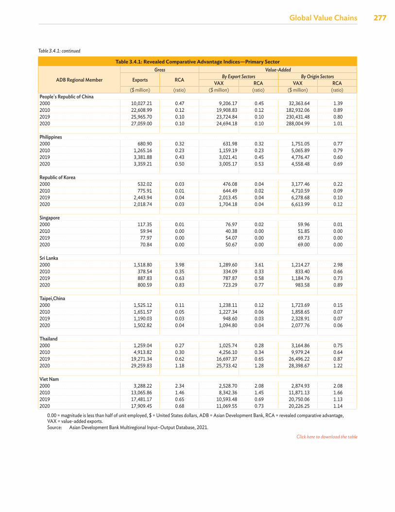
Global Value Chains
277Global Value Chains
Table 3.4.1: Revealed Comparative Advantage Indices—Primary Sector
ADB Regional Member
Gross Value-Added
Exports RCA By Export Sectors By Origin SectorsVAX RCA VAX RCA
($ million) (ratio) ($ million) (ratio) ($ million) (ratio)People's Republic of China2000 10,027.21 0.47 9,206.17 0.45 32,363.64 1.39 2010 22,608.99 0.12 19,908.83 0.12 182,932.06 0.89 2019 25,965.70 0.10 23,724.84 0.10 230,431.48 0.80 2020 27,059.00 0.10 24,694.18 0.10 288,004.99 1.01
Philippines2000 680.90 0.32 631.98 0.32 1,751.05 0.77 2010 1,265.16 0.23 1,159.19 0.23 5,065.89 0.79 2019 3,381.88 0.43 3,021.41 0.45 4,776.47 0.60 2020 3,359.21 0.50 3,005.17 0.53 4,558.48 0.69
Republic of Korea2000 532.02 0.03 476.08 0.04 3,177.46 0.22 2010 775.91 0.01 644.49 0.02 4,710.59 0.09 2019 2,443.94 0.04 2,013.45 0.04 6,278.68 0.10 2020 2,018.74 0.03 1,704.18 0.04 6,613.99 0.12
Singapore2000 117.35 0.01 76.97 0.02 59.96 0.01 2010 59.94 0.00 40.38 0.00 51.85 0.00 2019 77.97 0.00 54.07 0.00 69.73 0.00 2020 70.84 0.00 50.67 0.00 69.00 0.00
Sri Lanka2000 1,518.80 3.98 1,289.60 3.61 1,214.27 2.98 2010 378.54 0.35 334.09 0.33 833.40 0.66 2019 887.83 0.63 787.87 0.58 1,184.76 0.73 2020 800.59 0.83 723.29 0.77 983.58 0.89
Taipei,China2000 1,525.12 0.11 1,238.11 0.12 1,723.69 0.15 2010 1,651.57 0.05 1,227.34 0.06 1,858.65 0.07 2019 1,190.03 0.03 948.60 0.03 2,328.91 0.07 2020 1,502.82 0.04 1,094.80 0.04 2,077.76 0.06
Thailand2000 1,259.04 0.27 1,025.74 0.28 3,164.86 0.75 2010 4,913.82 0.30 4,256.10 0.34 9,979.24 0.64 2019 19,271.34 0.62 16,697.37 0.65 26,496.22 0.87 2020 29,259.83 1.18 25,733.42 1.28 28,398.67 1.22
Viet Nam2000 3,288.22 2.34 2,528.70 2.08 2,874.93 2.08 2010 13,065.86 1.46 8,342.36 1.45 11,871.13 1.66 2019 17,481.17 0.65 10,593.48 0.69 20,750.06 1.13 2020 17,909.45 0.68 11,069.55 0.73 20,226.25 1.14
0.00 = magnitude is less than half of unit employed, $ = United States dollars, ADB = Asian Development Bank, RCA = revealed comparative advantage, VAX = value-added exports.Source: Asian Development Bank Multiregional Input–Output Database, 2021.
Table 3.4.1: continued
Click here to download the table
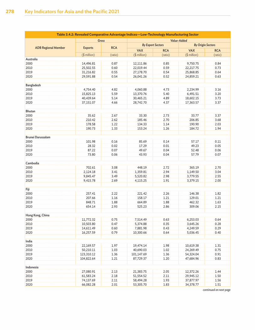
278 Key Indicators for Asia and the Pacific 2021
Table 3.4.2: Revealed Comparative Advantage Indices—Low-Technology Manufacturing Sector
ADB Regional Member
Gross Value-Added
Exports RCABy Export Sectors By Origin Sectors
VAX RCA VAX RCA($ million) (ratio) ($ million) (ratio) ($ million) (ratio)
Australia2000 14,496.81 0.87 12,111.86 0.85 9,750.75 0.84 2010 25,502.55 0.60 22,019.44 0.59 22,217.75 0.73 2019 31,216.82 0.55 27,178.70 0.54 25,868.85 0.64 2020 29,591.88 0.54 26,041.26 0.52 24,859.21 0.63
Bangladesh2000 4,754.40 4.82 4,060.88 4.73 2,234.99 3.16 2010 15,825.13 5.59 13,370.76 5.40 6,491.51 3.20 2019 40,439.64 5.14 30,465.21 4.89 18,602.15 3.73 2020 37,151.07 4.66 28,742.70 4.37 17,363.57 3.37
Bhutan2000 35.62 2.67 33.30 2.73 33.77 3.37 2010 210.42 2.62 185.46 2.70 206.85 3.68 2019 178.58 1.22 134.33 1.14 190.90 2.03 2020 190.73 1.33 153.24 1.26 184.72 1.94
Brunei Darussalam2000 101.98 0.16 85.69 0.14 57.17 0.11 2010 28.32 0.02 17.29 0.01 49.23 0.05 2019 87.22 0.07 49.67 0.04 52.48 0.06 2020 73.80 0.06 43.93 0.04 57.79 0.07
Cambodia2000 702.61 3.08 448.19 2.72 365.19 2.70 2010 2,124.18 3.41 1,359.81 2.94 1,149.50 3.04 2019 9,845.47 3.49 5,520.82 2.98 3,779.55 2.55 2020 9,415.78 2.69 4,115.25 1.91 3,379.15 2.00
Fiji2000 257.41 2.22 221.42 2.26 146.38 1.82 2010 207.66 1.16 158.17 1.21 129.01 1.21 2019 848.71 1.88 664.89 1.88 462.32 1.63 2020 654.14 2.93 525.23 2.86 309.06 2.15
Hong Kong, China2000 11,772.32 0.75 7,514.49 0.63 6,253.03 0.64 2010 10,503.80 0.47 5,374.88 0.35 3,645.26 0.28 2019 14,611.49 0.60 7,881.98 0.43 4,249.59 0.29 2020 16,257.59 0.79 10,300.66 0.64 5,036.45 0.40
India2000 22,169.57 1.97 19,474.14 1.98 10,619.38 1.31 2010 50,210.11 1.03 40,690.03 1.02 24,269.49 0.75 2019 123,310.12 1.36 101,147.69 1.36 54,324.04 0.91 2020 104,822.64 1.21 87,729.37 1.20 47,684.96 0.83
Indonesia2000 27,080.91 2.13 21,383.75 2.05 12,372.26 1.44 2010 61,583.24 2.18 51,554.52 2.11 29,945.12 1.50 2019 74,137.69 2.11 58,494.28 1.93 37,877.97 1.56 2020 66,082.28 2.01 53,305.70 1.83 34,378.77 1.51
continued on next page
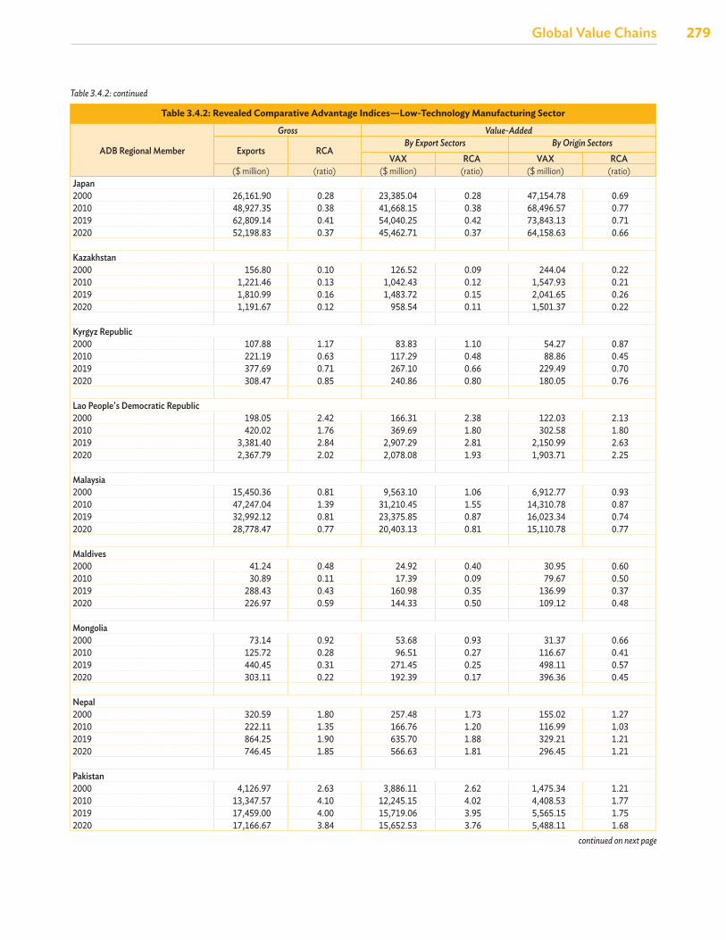
Global Value Chains
279Global Value Chains
Table 3.4.2: Revealed Comparative Advantage Indices—Low-Technology Manufacturing Sector
ADB Regional Member
Gross Value-Added
Exports RCABy Export Sectors By Origin Sectors
VAX RCA VAX RCA($ million) (ratio) ($ million) (ratio) ($ million) (ratio)
Japan2000 26,161.90 0.28 23,385.04 0.28 47,154.78 0.69 2010 48,927.35 0.38 41,668.15 0.38 68,496.57 0.77 2019 62,809.14 0.41 54,040.25 0.42 73,843.13 0.71 2020 52,198.83 0.37 45,462.71 0.37 64,158.63 0.66
Kazakhstan2000 156.80 0.10 126.52 0.09 244.04 0.22 2010 1,221.46 0.13 1,042.43 0.12 1,547.93 0.21 2019 1,810.99 0.16 1,483.72 0.15 2,041.65 0.26 2020 1,191.67 0.12 958.54 0.11 1,501.37 0.22
Kyrgyz Republic2000 107.88 1.17 83.83 1.10 54.27 0.87 2010 221.19 0.63 117.29 0.48 88.86 0.45 2019 377.69 0.71 267.10 0.66 229.49 0.70 2020 308.47 0.85 240.86 0.80 180.05 0.76
Lao People's Democratic Republic2000 198.05 2.42 166.31 2.38 122.03 2.13 2010 420.02 1.76 369.69 1.80 302.58 1.80 2019 3,381.40 2.84 2,907.29 2.81 2,150.99 2.63 2020 2,367.79 2.02 2,078.08 1.93 1,903.71 2.25
Malaysia2000 15,450.36 0.81 9,563.10 1.06 6,912.77 0.93 2010 47,247.04 1.39 31,210.45 1.55 14,310.78 0.87 2019 32,992.12 0.81 23,375.85 0.87 16,023.34 0.74 2020 28,778.47 0.77 20,403.13 0.81 15,110.78 0.77
Maldives2000 41.24 0.48 24.92 0.40 30.95 0.60 2010 30.89 0.11 17.39 0.09 79.67 0.50 2019 288.43 0.43 160.98 0.35 136.99 0.37 2020 226.97 0.59 144.33 0.50 109.12 0.48
Mongolia2000 73.14 0.92 53.68 0.93 31.37 0.66 2010 125.72 0.28 96.51 0.27 116.67 0.41 2019 440.45 0.31 271.45 0.25 498.11 0.57 2020 303.11 0.22 192.39 0.17 396.36 0.45
Nepal2000 320.59 1.80 257.48 1.73 155.02 1.27 2010 222.11 1.35 166.76 1.20 116.99 1.03 2019 864.25 1.90 635.70 1.88 329.21 1.21 2020 746.45 1.85 566.63 1.81 296.45 1.21
Pakistan2000 4,126.97 2.63 3,886.11 2.62 1,475.34 1.21 2010 13,347.57 4.10 12,245.15 4.02 4,408.53 1.77 2019 17,459.00 4.00 15,719.06 3.95 5,565.15 1.75 2020 17,166.67 3.84 15,652.53 3.76 5,488.11 1.68
continued on next page
Table 3.4.2: continued
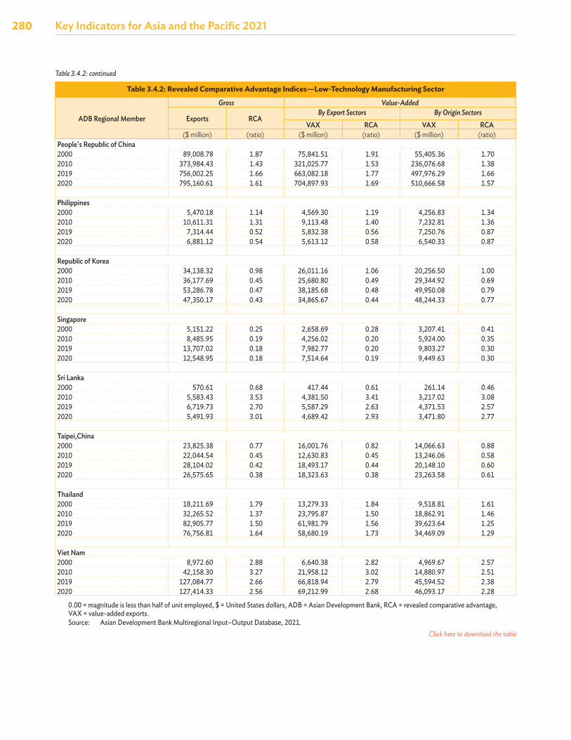
280 Key Indicators for Asia and the Pacific 2021
Table 3.4.2: Revealed Comparative Advantage Indices—Low-Technology Manufacturing Sector
ADB Regional Member
Gross Value-Added
Exports RCABy Export Sectors By Origin Sectors
VAX RCA VAX RCA($ million) (ratio) ($ million) (ratio) ($ million) (ratio)
People's Republic of China2000 89,008.78 1.87 75,841.51 1.91 55,405.36 1.70 2010 373,984.43 1.43 321,025.77 1.53 236,076.68 1.38 2019 756,002.25 1.66 663,082.18 1.77 497,976.29 1.66 2020 795,160.61 1.61 704,897.93 1.69 510,666.58 1.57
Philippines2000 5,470.18 1.14 4,569.30 1.19 4,256.83 1.34 2010 10,611.31 1.31 9,113.48 1.40 7,232.81 1.36 2019 7,314.44 0.52 5,832.38 0.56 7,250.76 0.87 2020 6,881.12 0.54 5,613.12 0.58 6,540.33 0.87
Republic of Korea2000 34,138.32 0.98 26,011.16 1.06 20,256.50 1.00 2010 36,177.69 0.45 25,680.80 0.49 29,344.92 0.69 2019 53,286.78 0.47 38,185.68 0.48 49,950.08 0.79 2020 47,350.17 0.43 34,865.67 0.44 48,244.33 0.77
Singapore2000 5,151.22 0.25 2,658.69 0.28 3,207.41 0.41 2010 8,485.95 0.19 4,256.02 0.20 5,924.00 0.35 2019 13,707.02 0.18 7,982.77 0.20 9,803.27 0.30 2020 12,548.95 0.18 7,514.64 0.19 9,449.63 0.30
Sri Lanka2000 570.61 0.68 417.44 0.61 261.14 0.46 2010 5,583.43 3.53 4,381.50 3.41 3,217.02 3.08 2019 6,719.73 2.70 5,587.29 2.63 4,371.53 2.57 2020 5,491.93 3.01 4,689.42 2.93 3,471.80 2.77
Taipei,China2000 23,825.38 0.77 16,001.76 0.82 14,066.63 0.88 2010 22,044.54 0.45 12,630.83 0.45 13,246.06 0.58 2019 28,104.02 0.42 18,493.17 0.44 20,148.10 0.60 2020 26,575.65 0.38 18,323.63 0.38 23,263.58 0.61
Thailand2000 18,211.69 1.79 13,279.33 1.84 9,518.81 1.61 2010 32,265.52 1.37 23,795.87 1.50 18,862.91 1.46 2019 82,905.77 1.50 61,981.79 1.56 39,623.64 1.25 2020 76,756.81 1.64 58,680.19 1.73 34,469.09 1.29
Viet Nam2000 8,972.60 2.88 6,640.38 2.82 4,969.67 2.57 2010 42,158.30 3.27 21,958.12 3.02 14,880.97 2.51 2019 127,084.77 2.66 66,818.94 2.79 45,594.52 2.38 2020 127,414.33 2.56 69,212.99 2.68 46,093.17 2.28
0.00 = magnitude is less than half of unit employed, $ = United States dollars, ADB = Asian Development Bank, RCA = revealed comparative advantage, VAX = value-added exports.Source: Asian Development Bank Multiregional Input–Output Database, 2021.
Table 3.4.2: continued
Click here to download the table
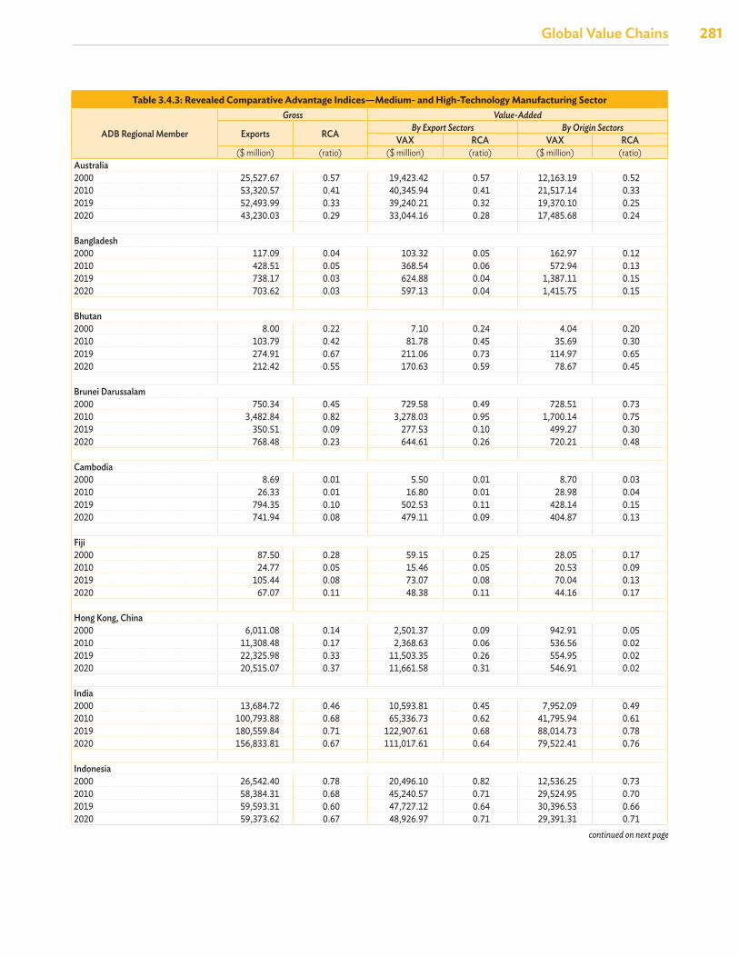
Global Value Chains
281Global Value Chains
Table 3.4.3: Revealed Comparative Advantage Indices—Medium- and High-Technology Manufacturing Sector
ADB Regional Member
Gross Value-Added
Exports RCA By Export Sectors By Origin SectorsVAX RCA VAX RCA
($ million) (ratio) ($ million) (ratio) ($ million) (ratio)Australia2000 25,527.67 0.57 19,423.42 0.57 12,163.19 0.52 2010 53,320.57 0.41 40,345.94 0.41 21,517.14 0.33 2019 52,493.99 0.33 39,240.21 0.32 19,370.10 0.25 2020 43,230.03 0.29 33,044.16 0.28 17,485.68 0.24
Bangladesh2000 117.09 0.04 103.32 0.05 162.97 0.12 2010 428.51 0.05 368.54 0.06 572.94 0.13 2019 738.17 0.03 624.88 0.04 1,387.11 0.15 2020 703.62 0.03 597.13 0.04 1,415.75 0.15
Bhutan2000 8.00 0.22 7.10 0.24 4.04 0.20 2010 103.79 0.42 81.78 0.45 35.69 0.30 2019 274.91 0.67 211.06 0.73 114.97 0.65 2020 212.42 0.55 170.63 0.59 78.67 0.45
Brunei Darussalam2000 750.34 0.45 729.58 0.49 728.51 0.73 2010 3,482.84 0.82 3,278.03 0.95 1,700.14 0.75 2019 350.51 0.09 277.53 0.10 499.27 0.30 2020 768.48 0.23 644.61 0.26 720.21 0.48
Cambodia2000 8.69 0.01 5.50 0.01 8.70 0.03 2010 26.33 0.01 16.80 0.01 28.98 0.04 2019 794.35 0.10 502.53 0.11 428.14 0.15 2020 741.94 0.08 479.11 0.09 404.87 0.13
Fiji2000 87.50 0.28 59.15 0.25 28.05 0.17 2010 24.77 0.05 15.46 0.05 20.53 0.09 2019 105.44 0.08 73.07 0.08 70.04 0.13 2020 67.07 0.11 48.38 0.11 44.16 0.17
Hong Kong, China2000 6,011.08 0.14 2,501.37 0.09 942.91 0.05 2010 11,308.48 0.17 2,368.63 0.06 536.56 0.02 2019 22,325.98 0.33 11,503.35 0.26 554.95 0.02 2020 20,515.07 0.37 11,661.58 0.31 546.91 0.02
India2000 13,684.72 0.46 10,593.81 0.45 7,952.09 0.49 2010 100,793.88 0.68 65,336.73 0.62 41,795.94 0.61 2019 180,559.84 0.71 122,907.61 0.68 88,014.73 0.78 2020 156,833.81 0.67 111,017.61 0.64 79,522.41 0.76
Indonesia2000 26,542.40 0.78 20,496.10 0.82 12,536.25 0.73 2010 58,384.31 0.68 45,240.57 0.71 29,524.95 0.70 2019 59,593.31 0.60 47,727.12 0.64 30,396.53 0.66 2020 59,373.62 0.67 48,926.97 0.71 29,391.31 0.71
continued on next page
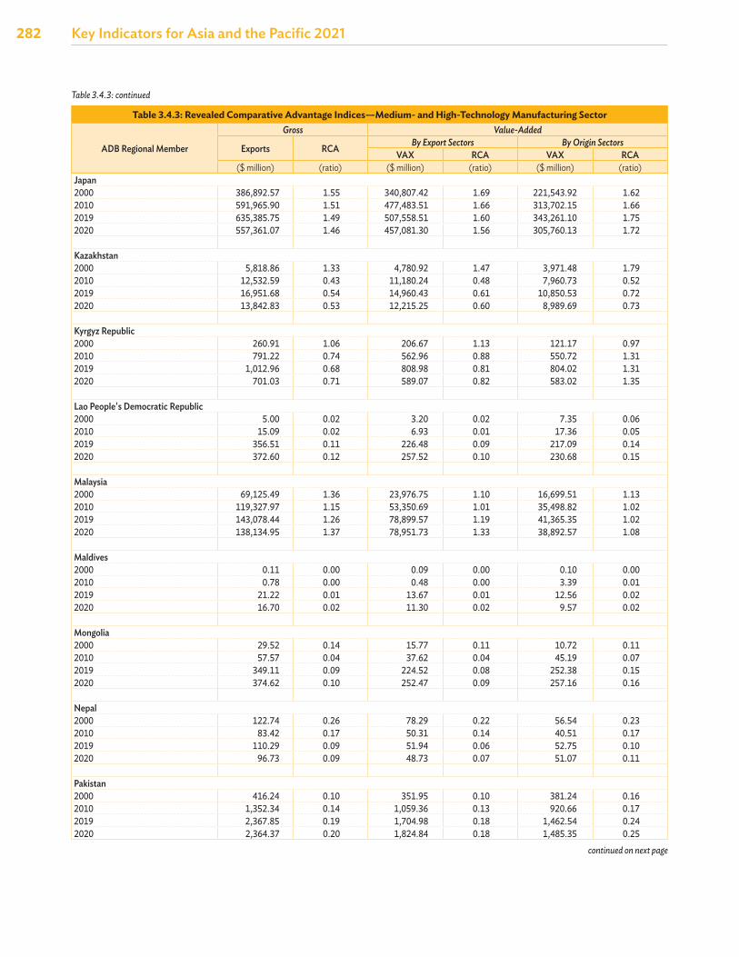
282 Key Indicators for Asia and the Pacific 2021
Table 3.4.3: Revealed Comparative Advantage Indices—Medium- and High-Technology Manufacturing Sector
ADB Regional Member
Gross Value-Added
Exports RCA By Export Sectors By Origin SectorsVAX RCA VAX RCA
($ million) (ratio) ($ million) (ratio) ($ million) (ratio)Japan2000 386,892.57 1.55 340,807.42 1.69 221,543.92 1.62 2010 591,965.90 1.51 477,483.51 1.66 313,702.15 1.66 2019 635,385.75 1.49 507,558.51 1.60 343,261.10 1.75 2020 557,361.07 1.46 457,081.30 1.56 305,760.13 1.72
Kazakhstan2000 5,818.86 1.33 4,780.92 1.47 3,971.48 1.79 2010 12,532.59 0.43 11,180.24 0.48 7,960.73 0.52 2019 16,951.68 0.54 14,960.43 0.61 10,850.53 0.72 2020 13,842.83 0.53 12,215.25 0.60 8,989.69 0.73
Kyrgyz Republic2000 260.91 1.06 206.67 1.13 121.17 0.97 2010 791.22 0.74 562.96 0.88 550.72 1.31 2019 1,012.96 0.68 808.98 0.81 804.02 1.31 2020 701.03 0.71 589.07 0.82 583.02 1.35
Lao People's Democratic Republic2000 5.00 0.02 3.20 0.02 7.35 0.06 2010 15.09 0.02 6.93 0.01 17.36 0.05 2019 356.51 0.11 226.48 0.09 217.09 0.14 2020 372.60 0.12 257.52 0.10 230.68 0.15
Malaysia2000 69,125.49 1.36 23,976.75 1.10 16,699.51 1.13 2010 119,327.97 1.15 53,350.69 1.01 35,498.82 1.02 2019 143,078.44 1.26 78,899.57 1.19 41,365.35 1.02 2020 138,134.95 1.37 78,951.73 1.33 38,892.57 1.08
Maldives2000 0.11 0.00 0.09 0.00 0.10 0.00 2010 0.78 0.00 0.48 0.00 3.39 0.01 2019 21.22 0.01 13.67 0.01 12.56 0.02 2020 16.70 0.02 11.30 0.02 9.57 0.02
Mongolia2000 29.52 0.14 15.77 0.11 10.72 0.11 2010 57.57 0.04 37.62 0.04 45.19 0.07 2019 349.11 0.09 224.52 0.08 252.38 0.15 2020 374.62 0.10 252.47 0.09 257.16 0.16
Nepal2000 122.74 0.26 78.29 0.22 56.54 0.23 2010 83.42 0.17 50.31 0.14 40.51 0.17 2019 110.29 0.09 51.94 0.06 52.75 0.10 2020 96.73 0.09 48.73 0.07 51.07 0.11
Pakistan2000 416.24 0.10 351.95 0.10 381.24 0.16 2010 1,352.34 0.14 1,059.36 0.13 920.66 0.17 2019 2,367.85 0.19 1,704.98 0.18 1,462.54 0.24 2020 2,364.37 0.20 1,824.84 0.18 1,485.35 0.25
continued on next page
Table 3.4.3: continued
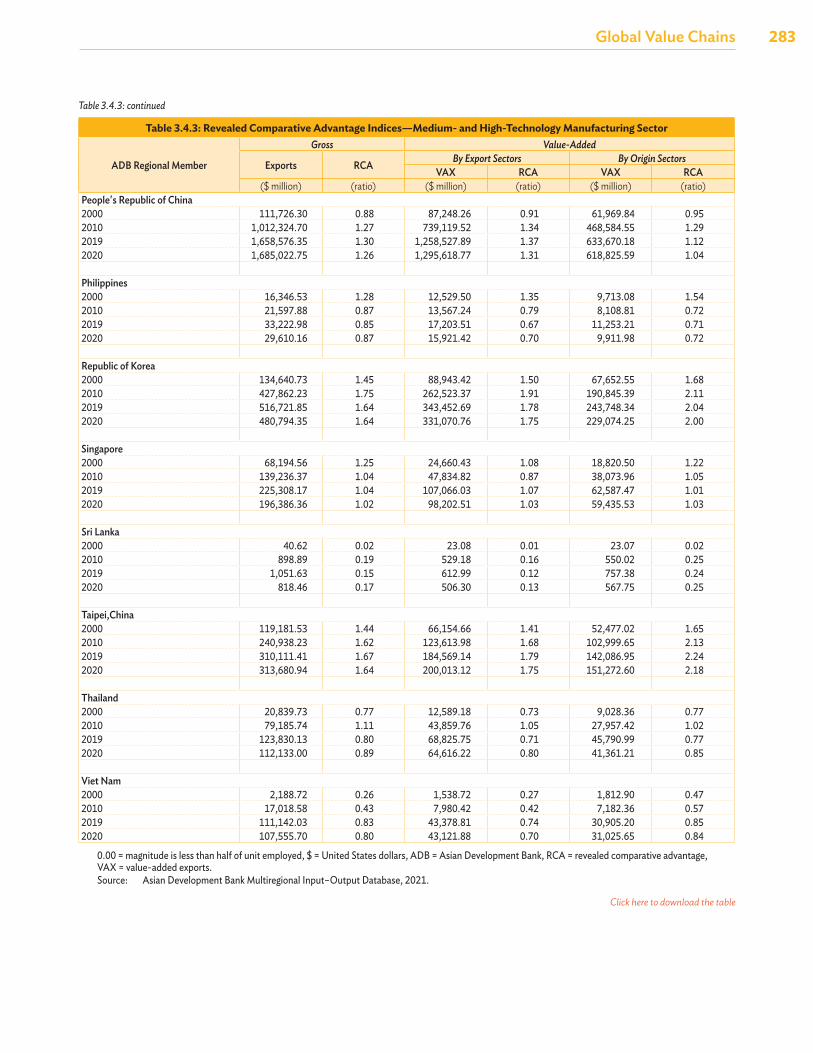
Global Value Chains
283Global Value Chains
Table 3.4.3: Revealed Comparative Advantage Indices—Medium- and High-Technology Manufacturing Sector
ADB Regional Member
Gross Value-Added
Exports RCA By Export Sectors By Origin SectorsVAX RCA VAX RCA
($ million) (ratio) ($ million) (ratio) ($ million) (ratio)People's Republic of China2000 111,726.30 0.88 87,248.26 0.91 61,969.84 0.95 2010 1,012,324.70 1.27 739,119.52 1.34 468,584.55 1.29 2019 1,658,576.35 1.30 1,258,527.89 1.37 633,670.18 1.12 2020 1,685,022.75 1.26 1,295,618.77 1.31 618,825.59 1.04
Philippines2000 16,346.53 1.28 12,529.50 1.35 9,713.08 1.54 2010 21,597.88 0.87 13,567.24 0.79 8,108.81 0.72 2019 33,222.98 0.85 17,203.51 0.67 11,253.21 0.71 2020 29,610.16 0.87 15,921.42 0.70 9,911.98 0.72
Republic of Korea2000 134,640.73 1.45 88,943.42 1.50 67,652.55 1.68 2010 427,862.23 1.75 262,523.37 1.91 190,845.39 2.11 2019 516,721.85 1.64 343,452.69 1.78 243,748.34 2.04 2020 480,794.35 1.64 331,070.76 1.75 229,074.25 2.00
Singapore2000 68,194.56 1.25 24,660.43 1.08 18,820.50 1.22 2010 139,236.37 1.04 47,834.82 0.87 38,073.96 1.05 2019 225,308.17 1.04 107,066.03 1.07 62,587.47 1.01 2020 196,386.36 1.02 98,202.51 1.03 59,435.53 1.03
Sri Lanka2000 40.62 0.02 23.08 0.01 23.07 0.02 2010 898.89 0.19 529.18 0.16 550.02 0.25 2019 1,051.63 0.15 612.99 0.12 757.38 0.24 2020 818.46 0.17 506.30 0.13 567.75 0.25
Taipei,China2000 119,181.53 1.44 66,154.66 1.41 52,477.02 1.65 2010 240,938.23 1.62 123,613.98 1.68 102,999.65 2.13 2019 310,111.41 1.67 184,569.14 1.79 142,086.95 2.24 2020 313,680.94 1.64 200,013.12 1.75 151,272.60 2.18
Thailand2000 20,839.73 0.77 12,589.18 0.73 9,028.36 0.77 2010 79,185.74 1.11 43,859.76 1.05 27,957.42 1.02 2019 123,830.13 0.80 68,825.75 0.71 45,790.99 0.77 2020 112,133.00 0.89 64,616.22 0.80 41,361.21 0.85
Viet Nam2000 2,188.72 0.26 1,538.72 0.27 1,812.90 0.47 2010 17,018.58 0.43 7,980.42 0.42 7,182.36 0.57 2019 111,142.03 0.83 43,378.81 0.74 30,905.20 0.85 2020 107,555.70 0.80 43,121.88 0.70 31,025.65 0.84
0.00 = magnitude is less than half of unit employed, $ = United States dollars, ADB = Asian Development Bank, RCA = revealed comparative advantage, VAX = value-added exports.Source: Asian Development Bank Multiregional Input–Output Database, 2021.
Table 3.4.3: continued
Click here to download the table
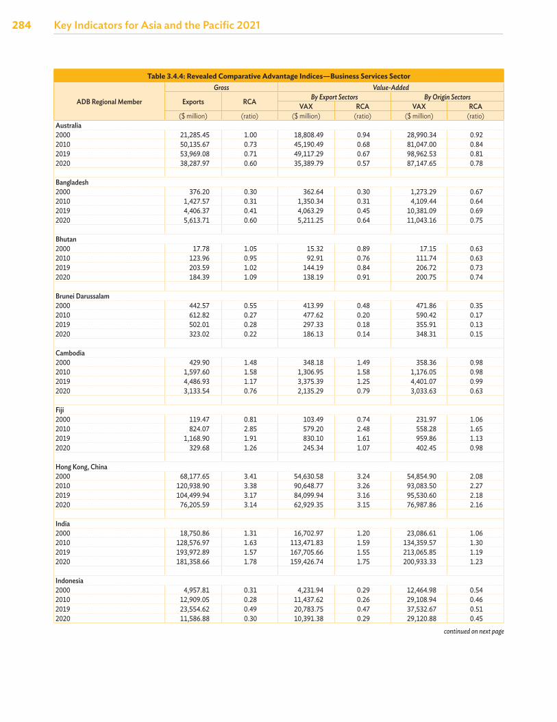
284 Key Indicators for Asia and the Pacific 2021
Table 3.4.4: Revealed Comparative Advantage Indices—Business Services Sector
ADB Regional Member
Gross Value-Added
Exports RCA By Export Sectors By Origin SectorsVAX RCA VAX RCA
($ million) (ratio) ($ million) (ratio) ($ million) (ratio)Australia2000 21,285.45 1.00 18,808.49 0.94 28,990.34 0.92 2010 50,135.67 0.73 45,190.49 0.68 81,047.00 0.84 2019 53,969.08 0.71 49,117.29 0.67 98,962.53 0.81 2020 38,287.97 0.60 35,389.79 0.57 87,147.65 0.78
Bangladesh2000 376.20 0.30 362.64 0.30 1,273.29 0.67 2010 1,427.57 0.31 1,350.34 0.31 4,109.44 0.64 2019 4,406.37 0.41 4,063.29 0.45 10,381.09 0.69 2020 5,613.71 0.60 5,211.25 0.64 11,043.16 0.75
Bhutan2000 17.78 1.05 15.32 0.89 17.15 0.63 2010 123.96 0.95 92.91 0.76 111.74 0.63 2019 203.59 1.02 144.19 0.84 206.72 0.73 2020 184.39 1.09 138.19 0.91 200.75 0.74
Brunei Darussalam2000 442.57 0.55 413.99 0.48 471.86 0.35 2010 612.82 0.27 477.62 0.20 590.42 0.17 2019 502.01 0.28 297.33 0.18 355.91 0.13 2020 323.02 0.22 186.13 0.14 348.31 0.15
Cambodia2000 429.90 1.48 348.18 1.49 358.36 0.98 2010 1,597.60 1.58 1,306.95 1.58 1,176.05 0.98 2019 4,486.93 1.17 3,375.39 1.25 4,401.07 0.99 2020 3,133.54 0.76 2,135.29 0.79 3,033.63 0.63
Fiji2000 119.47 0.81 103.49 0.74 231.97 1.06 2010 824.07 2.85 579.20 2.48 558.28 1.65 2019 1,168.90 1.91 830.10 1.61 959.86 1.13 2020 329.68 1.26 245.34 1.07 402.45 0.98
Hong Kong, China2000 68,177.65 3.41 54,630.58 3.24 54,854.90 2.08 2010 120,938.90 3.38 90,648.77 3.26 93,083.50 2.27 2019 104,499.94 3.17 84,099.94 3.16 95,530.60 2.18 2020 76,205.59 3.14 62,929.35 3.15 76,987.86 2.16
India2000 18,750.86 1.31 16,702.97 1.20 23,086.61 1.06 2010 128,576.97 1.63 113,471.83 1.59 134,359.57 1.30 2019 193,972.89 1.57 167,705.66 1.55 213,065.85 1.19 2020 181,358.66 1.78 159,426.74 1.75 200,933.33 1.23
Indonesia2000 4,957.81 0.31 4,231.94 0.29 12,464.98 0.54 2010 12,909.05 0.28 11,437.62 0.26 29,108.94 0.46 2019 23,554.62 0.49 20,783.75 0.47 37,532.67 0.51 2020 11,586.88 0.30 10,391.38 0.29 29,120.88 0.45
continued on next page
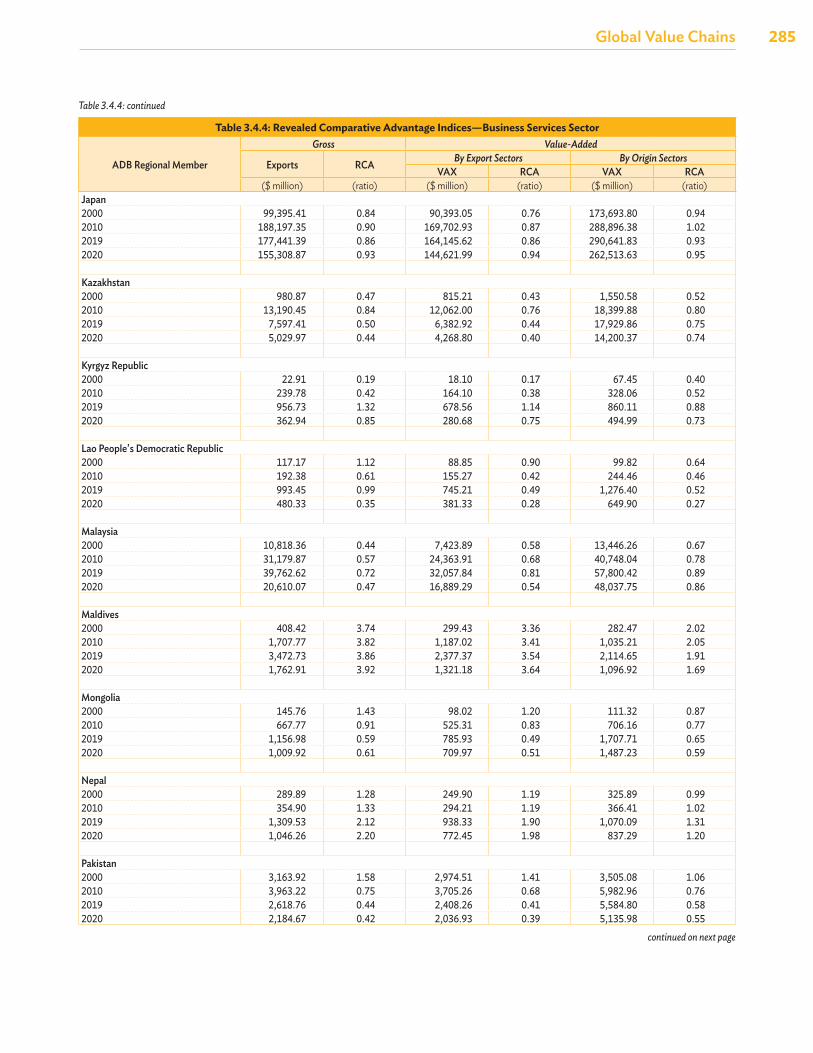
Global Value Chains
285Global Value Chains
Table 3.4.4: Revealed Comparative Advantage Indices—Business Services Sector
ADB Regional Member
Gross Value-Added
Exports RCA By Export Sectors By Origin SectorsVAX RCA VAX RCA
($ million) (ratio) ($ million) (ratio) ($ million) (ratio)Japan2000 99,395.41 0.84 90,393.05 0.76 173,693.80 0.94 2010 188,197.35 0.90 169,702.93 0.87 288,896.38 1.02 2019 177,441.39 0.86 164,145.62 0.86 290,641.83 0.93 2020 155,308.87 0.93 144,621.99 0.94 262,513.63 0.95
Kazakhstan2000 980.87 0.47 815.21 0.43 1,550.58 0.52 2010 13,190.45 0.84 12,062.00 0.76 18,399.88 0.80 2019 7,597.41 0.50 6,382.92 0.44 17,929.86 0.75 2020 5,029.97 0.44 4,268.80 0.40 14,200.37 0.74
Kyrgyz Republic2000 22.91 0.19 18.10 0.17 67.45 0.40 2010 239.78 0.42 164.10 0.38 328.06 0.52 2019 956.73 1.32 678.56 1.14 860.11 0.88 2020 362.94 0.85 280.68 0.75 494.99 0.73
Lao People's Democratic Republic2000 117.17 1.12 88.85 0.90 99.82 0.64 2010 192.38 0.61 155.27 0.42 244.46 0.46 2019 993.45 0.99 745.21 0.49 1,276.40 0.52 2020 480.33 0.35 381.33 0.28 649.90 0.27
Malaysia2000 10,818.36 0.44 7,423.89 0.58 13,446.26 0.67 2010 31,179.87 0.57 24,363.91 0.68 40,748.04 0.78 2019 39,762.62 0.72 32,057.84 0.81 57,800.42 0.89 2020 20,610.07 0.47 16,889.29 0.54 48,037.75 0.86
Maldives2000 408.42 3.74 299.43 3.36 282.47 2.02 2010 1,707.77 3.82 1,187.02 3.41 1,035.21 2.05 2019 3,472.73 3.86 2,377.37 3.54 2,114.65 1.91 2020 1,762.91 3.92 1,321.18 3.64 1,096.92 1.69
Mongolia2000 145.76 1.43 98.02 1.20 111.32 0.87 2010 667.77 0.91 525.31 0.83 706.16 0.77 2019 1,156.98 0.59 785.93 0.49 1,707.71 0.65 2020 1,009.92 0.61 709.97 0.51 1,487.23 0.59
Nepal2000 289.89 1.28 249.90 1.19 325.89 0.99 2010 354.90 1.33 294.21 1.19 366.41 1.02 2019 1,309.53 2.12 938.33 1.90 1,070.09 1.31 2020 1,046.26 2.20 772.45 1.98 837.29 1.20
Pakistan2000 3,163.92 1.58 2,974.51 1.41 3,505.08 1.06 2010 3,963.22 0.75 3,705.26 0.68 5,982.96 0.76 2019 2,618.76 0.44 2,408.26 0.41 5,584.80 0.58 2020 2,184.67 0.42 2,036.93 0.39 5,135.98 0.55
Table 3.4.4: continued
continued on next page
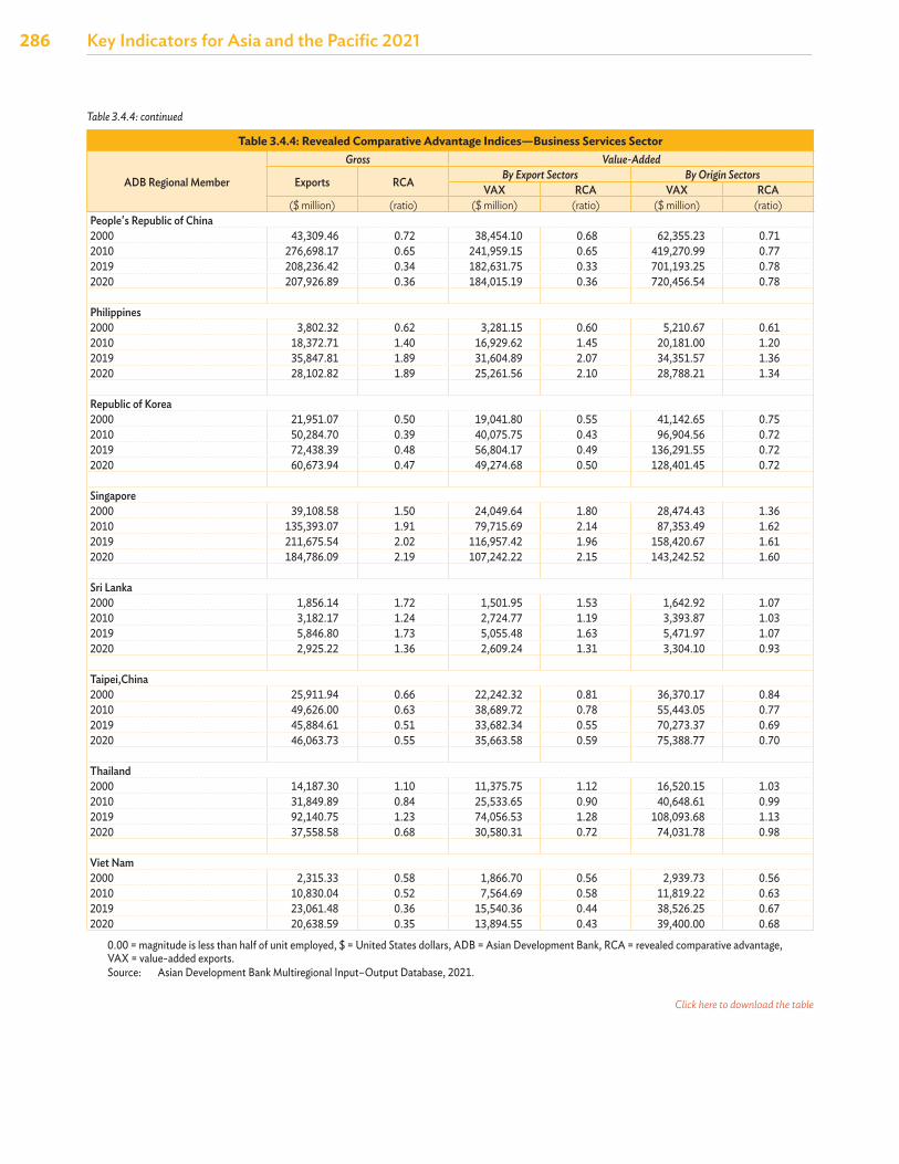
286 Key Indicators for Asia and the Pacific 2021
Table 3.4.4: Revealed Comparative Advantage Indices—Business Services Sector
ADB Regional Member
Gross Value-Added
Exports RCA By Export Sectors By Origin SectorsVAX RCA VAX RCA
($ million) (ratio) ($ million) (ratio) ($ million) (ratio)People's Republic of China2000 43,309.46 0.72 38,454.10 0.68 62,355.23 0.71 2010 276,698.17 0.65 241,959.15 0.65 419,270.99 0.77 2019 208,236.42 0.34 182,631.75 0.33 701,193.25 0.78 2020 207,926.89 0.36 184,015.19 0.36 720,456.54 0.78
Philippines2000 3,802.32 0.62 3,281.15 0.60 5,210.67 0.61 2010 18,372.71 1.40 16,929.62 1.45 20,181.00 1.20 2019 35,847.81 1.89 31,604.89 2.07 34,351.57 1.36 2020 28,102.82 1.89 25,261.56 2.10 28,788.21 1.34
Republic of Korea2000 21,951.07 0.50 19,041.80 0.55 41,142.65 0.75 2010 50,284.70 0.39 40,075.75 0.43 96,904.56 0.72 2019 72,438.39 0.48 56,804.17 0.49 136,291.55 0.72 2020 60,673.94 0.47 49,274.68 0.50 128,401.45 0.72
Singapore2000 39,108.58 1.50 24,049.64 1.80 28,474.43 1.36 2010 135,393.07 1.91 79,715.69 2.14 87,353.49 1.62 2019 211,675.54 2.02 116,957.42 1.96 158,420.67 1.61 2020 184,786.09 2.19 107,242.22 2.15 143,242.52 1.60
Sri Lanka2000 1,856.14 1.72 1,501.95 1.53 1,642.92 1.07 2010 3,182.17 1.24 2,724.77 1.19 3,393.87 1.03 2019 5,846.80 1.73 5,055.48 1.63 5,471.97 1.07 2020 2,925.22 1.36 2,609.24 1.31 3,304.10 0.93
Taipei,China2000 25,911.94 0.66 22,242.32 0.81 36,370.17 0.84 2010 49,626.00 0.63 38,689.72 0.78 55,443.05 0.77 2019 45,884.61 0.51 33,682.34 0.55 70,273.37 0.69 2020 46,063.73 0.55 35,663.58 0.59 75,388.77 0.70
Thailand2000 14,187.30 1.10 11,375.75 1.12 16,520.15 1.03 2010 31,849.89 0.84 25,533.65 0.90 40,648.61 0.99 2019 92,140.75 1.23 74,056.53 1.28 108,093.68 1.13 2020 37,558.58 0.68 30,580.31 0.72 74,031.78 0.98
Viet Nam2000 2,315.33 0.58 1,866.70 0.56 2,939.73 0.56 2010 10,830.04 0.52 7,564.69 0.58 11,819.22 0.63 2019 23,061.48 0.36 15,540.36 0.44 38,526.25 0.67 2020 20,638.59 0.35 13,894.55 0.43 39,400.00 0.68
0.00 = magnitude is less than half of unit employed, $ = United States dollars, ADB = Asian Development Bank, RCA = revealed comparative advantage, VAX = value-added exports.Source: Asian Development Bank Multiregional Input–Output Database, 2021.
Table 3.4.4: continued
Click here to download the table
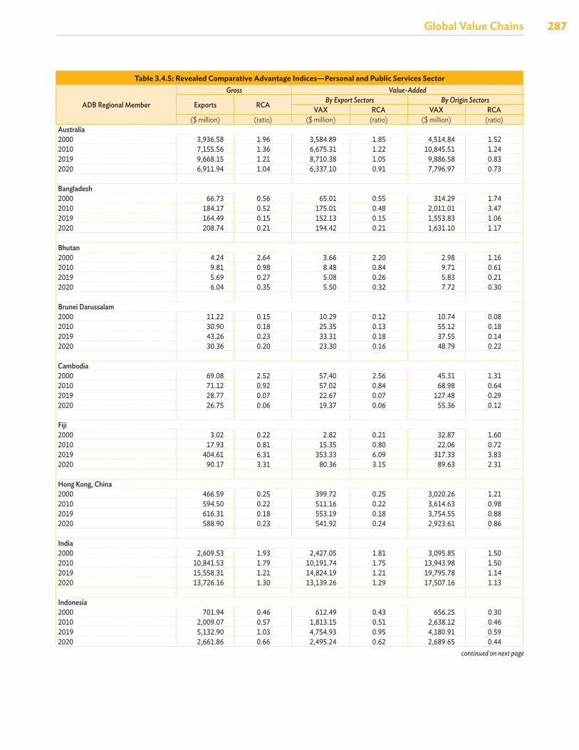
Global Value Chains
287Global Value Chains
Table 3.4.5: Revealed Comparative Advantage Indices—Personal and Public Services Sector
ADB Regional Member
Gross Value-Added
Exports RCA By Export Sectors By Origin SectorsVAX RCA VAX RCA
($ million) (ratio) ($ million) (ratio) ($ million) (ratio)Australia2000 3,936.58 1.96 3,584.89 1.85 4,514.84 1.52 2010 7,155.56 1.36 6,675.31 1.22 10,845.51 1.24 2019 9,668.15 1.21 8,710.38 1.05 9,886.58 0.83 2020 6,911.94 1.04 6,337.10 0.91 7,796.97 0.73
Bangladesh2000 66.73 0.56 65.01 0.55 314.29 1.74 2010 184.17 0.52 175.01 0.48 2,011.01 3.47 2019 164.49 0.15 152.13 0.15 1,553.83 1.06 2020 208.74 0.21 194.42 0.21 1,631.10 1.17
Bhutan2000 4.24 2.64 3.66 2.20 2.98 1.16 2010 9.81 0.98 8.48 0.84 9.71 0.61 2019 5.69 0.27 5.08 0.26 5.83 0.21 2020 6.04 0.35 5.50 0.32 7.72 0.30
Brunei Darussalam2000 11.22 0.15 10.29 0.12 10.74 0.08 2010 30.90 0.18 25.35 0.13 55.12 0.18 2019 43.26 0.23 33.31 0.18 37.55 0.14 2020 30.36 0.20 23.30 0.16 48.79 0.22
Cambodia2000 69.08 2.52 57.40 2.56 45.31 1.31 2010 71.12 0.92 57.02 0.84 68.98 0.64 2019 28.77 0.07 22.67 0.07 127.48 0.29 2020 26.75 0.06 19.37 0.06 55.36 0.12
Fiji2000 3.02 0.22 2.82 0.21 32.87 1.60 2010 17.93 0.81 15.35 0.80 22.06 0.72 2019 404.61 6.31 353.33 6.09 317.33 3.83 2020 90.17 3.31 80.36 3.15 89.63 2.31
Hong Kong, China2000 466.59 0.25 399.72 0.25 3,020.26 1.21 2010 594.50 0.22 511.16 0.22 3,614.63 0.98 2019 616.31 0.18 553.19 0.18 3,754.55 0.88 2020 588.90 0.23 541.92 0.24 2,923.61 0.86
India2000 2,609.53 1.93 2,427.05 1.81 3,095.85 1.50 2010 10,841.53 1.79 10,191.74 1.75 13,943.98 1.50 2019 15,558.31 1.21 14,824.19 1.21 19,795.78 1.14 2020 13,726.16 1.30 13,139.26 1.29 17,507.16 1.13
Indonesia2000 701.94 0.46 612.49 0.43 656.25 0.30 2010 2,009.07 0.57 1,813.15 0.51 2,638.12 0.46 2019 5,132.90 1.03 4,754.93 0.95 4,180.91 0.59 2020 2,661.86 0.66 2,495.24 0.62 2,689.65 0.44
continued on next page
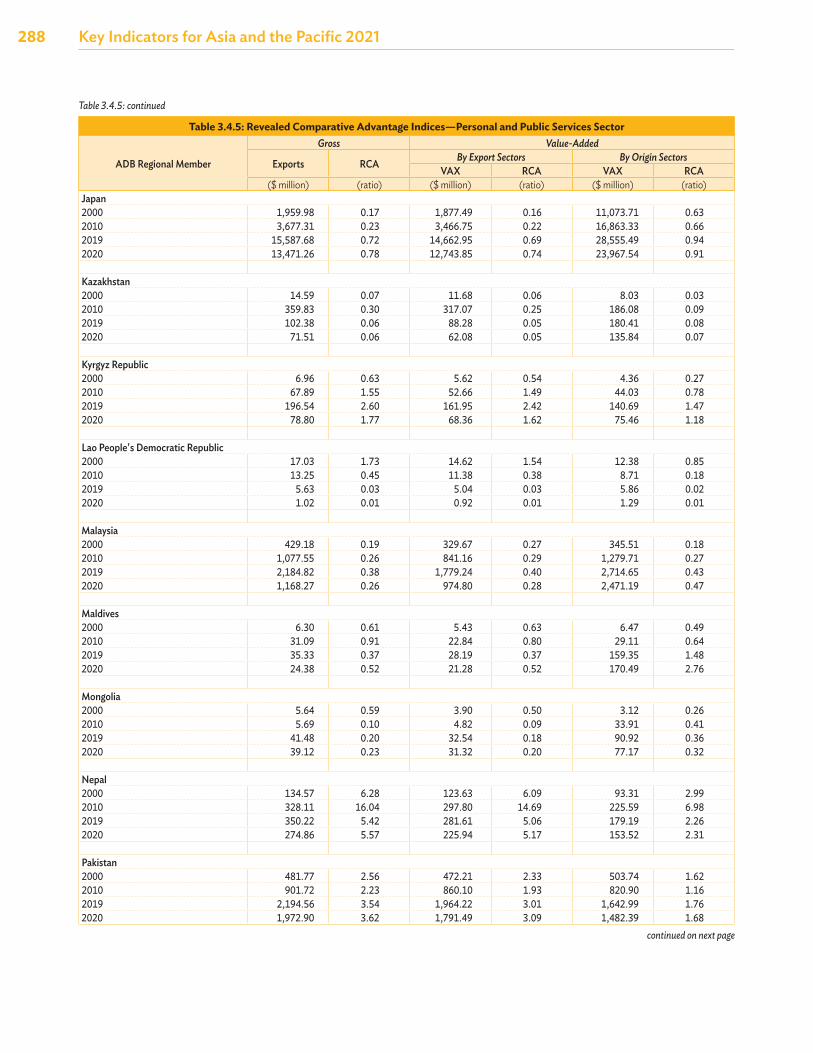
288 Key Indicators for Asia and the Pacific 2021
Table 3.4.5: Revealed Comparative Advantage Indices—Personal and Public Services Sector
ADB Regional Member
Gross Value-Added
Exports RCA By Export Sectors By Origin SectorsVAX RCA VAX RCA
($ million) (ratio) ($ million) (ratio) ($ million) (ratio)Japan2000 1,959.98 0.17 1,877.49 0.16 11,073.71 0.63 2010 3,677.31 0.23 3,466.75 0.22 16,863.33 0.66 2019 15,587.68 0.72 14,662.95 0.69 28,555.49 0.94 2020 13,471.26 0.78 12,743.85 0.74 23,967.54 0.91
Kazakhstan2000 14.59 0.07 11.68 0.06 8.03 0.03 2010 359.83 0.30 317.07 0.25 186.08 0.09 2019 102.38 0.06 88.28 0.05 180.41 0.08 2020 71.51 0.06 62.08 0.05 135.84 0.07
Kyrgyz Republic2000 6.96 0.63 5.62 0.54 4.36 0.27 2010 67.89 1.55 52.66 1.49 44.03 0.78 2019 196.54 2.60 161.95 2.42 140.69 1.47 2020 78.80 1.77 68.36 1.62 75.46 1.18
Lao People's Democratic Republic2000 17.03 1.73 14.62 1.54 12.38 0.85 2010 13.25 0.45 11.38 0.38 8.71 0.18 2019 5.63 0.03 5.04 0.03 5.86 0.02 2020 1.02 0.01 0.92 0.01 1.29 0.01
Malaysia2000 429.18 0.19 329.67 0.27 345.51 0.18 2010 1,077.55 0.26 841.16 0.29 1,279.71 0.27 2019 2,184.82 0.38 1,779.24 0.40 2,714.65 0.43 2020 1,168.27 0.26 974.80 0.28 2,471.19 0.47
Maldives2000 6.30 0.61 5.43 0.63 6.47 0.49 2010 31.09 0.91 22.84 0.80 29.11 0.64 2019 35.33 0.37 28.19 0.37 159.35 1.48 2020 24.38 0.52 21.28 0.52 170.49 2.76
Mongolia2000 5.64 0.59 3.90 0.50 3.12 0.26 2010 5.69 0.10 4.82 0.09 33.91 0.41 2019 41.48 0.20 32.54 0.18 90.92 0.36 2020 39.12 0.23 31.32 0.20 77.17 0.32
Nepal2000 134.57 6.28 123.63 6.09 93.31 2.99 2010 328.11 16.04 297.80 14.69 225.59 6.98 2019 350.22 5.42 281.61 5.06 179.19 2.26 2020 274.86 5.57 225.94 5.17 153.52 2.31
Pakistan2000 481.77 2.56 472.21 2.33 503.74 1.62 2010 901.72 2.23 860.10 1.93 820.90 1.16 2019 2,194.56 3.54 1,964.22 3.01 1,642.99 1.76 2020 1,972.90 3.62 1,791.49 3.09 1,482.39 1.68
continued on next page
Table 3.4.5: continued
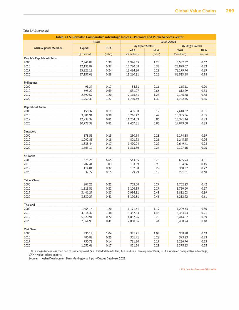
Global Value Chains
289Global Value Chains
Table 3.4.5: Revealed Comparative Advantage Indices—Personal and Public Services Sector
ADB Regional Member
Gross Value-Added
Exports RCA By Export Sectors By Origin SectorsVAX RCA VAX RCA
($ million) (ratio) ($ million) (ratio) ($ million) (ratio)People's Republic of China2000 7,945.89 1.39 6,926.55 1.28 5,582.52 0.67 2010 12,135.87 0.37 10,730.08 0.35 25,879.07 0.53 2019 15,322.12 0.24 13,484.30 0.22 78,179.74 0.89 2020 17,157.06 0.28 15,260.81 0.26 86,533.18 0.98
Philippines2000 95.37 0.17 84.81 0.16 165.11 0.20 2010 695.20 0.69 631.27 0.66 812.29 0.53 2019 2,390.59 1.20 2,116.61 1.23 2,146.78 0.88 2020 1,959.43 1.27 1,750.49 1.30 1,752.75 0.86
Republic of Korea2000 450.37 0.11 405.30 0.12 2,648.62 0.51 2010 3,801.91 0.38 3,216.42 0.42 10,335.36 0.85 2019 12,933.32 0.81 11,204.09 0.86 15,391.44 0.83 2020 10,777.32 0.81 9,467.81 0.85 14,049.08 0.83
Singapore2000 378.55 0.15 290.94 0.23 1,174.38 0.59 2010 1,002.85 0.18 801.93 0.26 1,245.55 0.26 2019 1,838.44 0.17 1,470.24 0.22 2,649.41 0.28 2020 1,603.17 0.18 1,313.80 0.24 2,127.16 0.25
Sri Lanka2000 675.26 6.65 543.35 5.78 655.94 4.51 2010 202.41 1.03 183.09 0.98 134.36 0.45 2019 114.01 0.32 102.38 0.29 360.37 0.72 2020 32.77 0.15 29.99 0.13 231.01 0.68
Taipei,China2000 807.26 0.22 703.00 0.27 1,702.33 0.42 2010 1,313.56 0.22 1,106.15 0.27 3,720.60 0.57 2019 3,441.27 0.37 2,956.11 0.43 5,812.03 0.59 2020 3,530.27 0.41 3,120.51 0.46 6,212.92 0.61
Thailand2000 1,464.14 1.20 1,171.61 1.19 1,209.43 0.80 2010 4,016.49 1.38 3,387.04 1.46 3,384.24 0.91 2019 5,620.91 0.72 4,887.96 0.75 6,444.87 0.69 2020 2,364.99 0.41 2,080.86 0.44 3,430.24 0.48
Viet Nam2000 390.19 1.04 331.71 1.03 308.98 0.63 2010 400.82 0.25 301.41 0.28 393.33 0.23 2019 950.78 0.14 731.20 0.19 1,286.76 0.23 2020 1,052.66 0.17 821.24 0.23 1,375.13 0.25
0.00 = magnitude is less than half of unit employed, $ = United States dollars, ADB = Asian Development Bank, RCA = revealed comparative advantage, VAX = value-added exports.Source: Asian Development Bank Multiregional Input–Output Database, 2021.
Table 3.4.5: continued
Click here to download the table