Part II: Sample Preparation for AFM Particle Characterization

Natasha Starostina, Paul West

Pacific Nanotechnology, Inc.3350 Scott Blvd., Suite 29

Santa Clara, CA 95054www.nanoparticles.pacificnanotech.com

Revision.1/16/06.A

Part II: Sample Preparation for AFM Particle Characterization 1

Revision.1/16/06.A

Introduction

Over the past 20 years Scanning Probe Microscopes (SPM) have emerged as an essential material characterization technique in various fields1,2,3,4,5. The importance of the SPM was evident as early as 1984 when the Nobel prize was awarded for the Scanning Tunneling Microscope (STM) invention by IBM researchers1. Today the Atomic Force Microscope (AFM) is the most commonly used scanning probe technique for materials characterization2. Major advantages of AFM are that it has a combination of high resolution in three dimensions, the sample does not have to be conductive, and there is no requirement for operation within a vacuum.

With an AFM, a large range of topographies and many types of materials can be imaged. Examples of surface features that may be imaged include: atomic terraces, carbon nanotubes, colloidal particles, viruses, DVD textures up to micro lens textures, fractured surfaces, and complex multi-phase polymers. In other words, AFM is capable of delivering unique 3D topography information from the angstrom level to the micron scale with unprecedented resolution.

With an AFM, the Z-axis resolution (i.e., perpendicular to the surface) is typically better than the resolution in the XY scan plane of the sample surface. Under ambient conditions, the Z-resolution for most of the commercially available AFMs is on the sub-angstrom level. Resolution in the X-Y scan place is oftern limited by the diameter of the probe and is on the order of a few nanometers. In the X and Y ases, AFM images are always a convolution of the probe geometry and sample texture. However, if the probe is much smaller than the surface features, the image distortions introduced by the probe are minimal.

The extreme sensitivity of the AFM is derived from a force sensor that measures forces between the probe and target surface which are typically less than 1 nN/nm. Most AFM’s utilize a light lever or a force sensor, as first disclosed in 1929 and then applied to the AFM in 1986. Figure 1 shows a schematic of the AFM. Recently, a new type of force sensor, based on a crystal resonator, shows promise for making the AFM much simpler to operate6,7 and it provides a very high force sensitivity required for high resolution imaging.

Figure 1: Schematic of AFM

Laser

Cantilever

Photo Detector

So

Differential Amplifier

Sample

Natasha Starostina, Paul WestPacific Nanotechnology3350 Scott Blvd.Santa Clara, CA 95054

Abstract

Scanning Probe Microscopy has been routinely employed as a surface characterization technique for nearly 20 years. Atomic Force Microscopy is the most widely used subset of SPM, which can be used in ambient conditions with minimum sample preparation. AFM is able to measure three-dimensional topography information from the angstrom level to the micron scale with unprecedented resolution. This paper reviews the most common methods of sample preparation that are used for imaging nanoparticles with an AFM. AFM is well suited to individual particle characterization. The standard set of measured parameters includes: volume, height, size, shape, aspect ratio and particle surface morphology. As a single-particle technique, physical parameters for each particle in an image can be recorded and the data set can be processed to generate a statistical distribution for an entire set of particles (i.e. ensemble-like information). Speeding up the process of obtaining data is critical for many reasons and definitely makes AFM more attractive given its ability of individual particle imaging. In general, the AFM particle characterization is both cost and time effective as well as easier to use than electron microscopy. The resolution of AFM is greater or comparable to that of SEM/TEM, and strong advantages of AFM for particle characterization include direct measurements of height, volume and 3D display.

Part II: Sample Preparation for AFM Particle Characterization 2

Revision.1/16/06.A

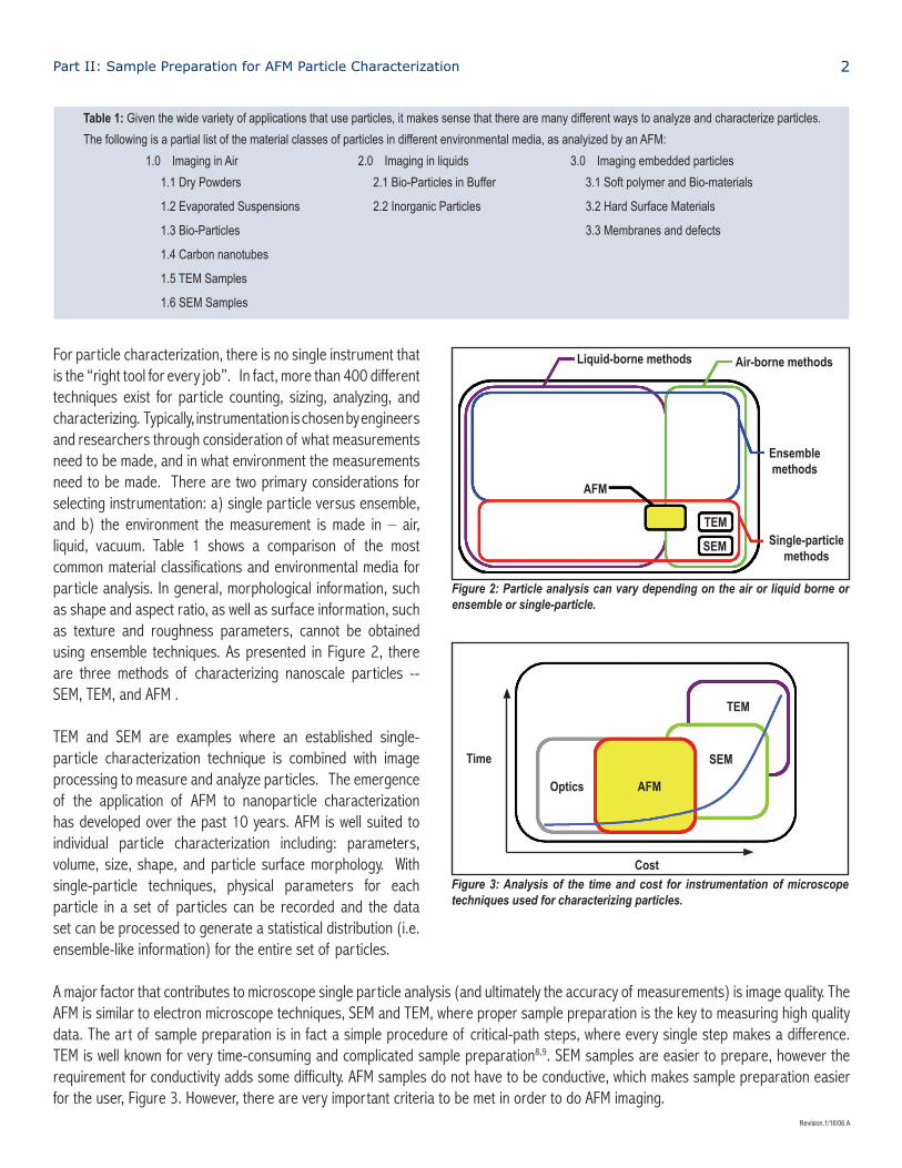
For particle characterization, there is no single instrument that is the “right tool for every job”. In fact, more than 400 different techniques exist for particle counting, sizing, analyzing, and characterizing. Typically, instrumentation is chosen by engineers and researchers through consideration of what measurements need to be made, and in what environment the measurements need to be made. There are two primary considerations for selecting instrumentation: a) single particle versus ensemble, and b) the environment the measurement is made in – air, liquid, vacuum. Table 1 shows a comparison of the most common material classifications and environmental media for particle analysis. In general, morphological information, such as shape and aspect ratio, as well as surface information, such as texture and roughness parameters, cannot be obtained using ensemble techniques. As presented in Figure 2, there are three methods of characterizing nanoscale particles -- SEM, TEM, and AFM .

TEM and SEM are examples where an established single-particle characterization technique is combined with image processing to measure and analyze particles. The emergence of the application of AFM to nanoparticle characterization has developed over the past 10 years. AFM is well suited to individual particle characterization including: parameters, volume, size, shape, and particle surface morphology. With single-particle techniques, physical parameters for each particle in a set of particles can be recorded and the data set can be processed to generate a statistical distribution (i.e. ensemble-like information) for the entire set of particles.

A major factor that contributes to microscope single particle analysis (and ultimately the accuracy of measurements) is image quality. The AFM is similar to electron microscope techniques, SEM and TEM, where proper sample preparation is the key to measuring high quality data. The art of sample preparation is in fact a simple procedure of critical-path steps, where every single step makes a difference. TEM is well known for very time-consuming and complicated sample preparation8,9. SEM samples are easier to prepare, however the requirement for conductivity adds some difficulty. AFM samples do not have to be conductive, which makes sample preparation easier for the user, Figure 3. However, there are very important criteria to be met in order to do AFM imaging.

Figure 2: Particle analysis can vary depending on the air or liquid borne or ensemble or single-particle.

Liquid-borne methods Air-borne methods

Ensemblemethods

Single-particlemethods

AFM

TEM

SEM

Figure 3: Analysis of the time and cost for instrumentation of microscope techniques used for characterizing particles.

Optics

Time

Cost

AFM

SEM

TEM

Table 1: Given the wide variety of applications that use particles, it makes sense that there are many different ways to analyze and characterize particles.

The following is a partial list of the material classes of particles in different environmental media, as analyized by an AFM:

1.0 Imaging in Air 2.0 Imaging in liquids 3.0 Imaging embedded particles

1.1 Dry Powders 2.1 Bio-Particles in Buffer 3.1 Soft polymer and Bio-materials

1.2 Evaporated Suspensions 2.2 Inorganic Particles 3.2 Hard Surface Materials

1.3 Bio-Particles 3.3 Membranes and defects

1.4 Carbon nanotubes

1.5 TEM Samples

1.6 SEM Samples

Part II: Sample Preparation for AFM Particle Characterization 3

Revision.1/16/06.A

The main focus of this article is to present a general survey of AFM sample preparation methods for nanoparticle characterization. The authors present a review of the available methods for AFM particle imaging and characterization in ambient conditions and in liquids. When available, references for additional information are provided. All AFM images shown is this paper have been obtained on a Light Lever or Crystal Nano-RP™ AFM. Close contact mode is the imaging mode for all images scanned in air this paper.

Particles, Dispersion, Substrates, Adhesives

The vast variety of particles can be categorized as engineered and non-engineered environmental particles. Engineered or artificially created particles break down to organic and inorganic categories. Those categories in turn have additional subdivisions, for example powders, suspensions and embedded particles. Different approaches can be used to prepare AFM samples10-16. Particle size, hydrophobicity, native environment and bio-compatibility are taken into consideration.

AFM particle imaging requires that: a) The particles to be rigidly adhered to a substrate. b) The particles to be dispersed on a the substrate. c) The substrate roughness is less than the size of the nanoparticles .

Often an adhesive is required for affixing the nanoparticles on a substrate. There are a large number of adhesive choices of the adhesive for small particle deposition. The most commonly used chemicals are poly-l-lysine, poly-D-lysine17, PEI (poly-ethyleneimide) or APTES (aminopropyltriethoxy silane) to facilitate chemical bonding between particle and substrate. Functionalized surfaces might either promote adsorption or allow covalent bonding. Sometimes hydrophobic substrates are preferable in air-AFM, this way formation of a water monolayer can be avoided12. HPOG or spin-coating of polymers is a convenient method for creating hydrophobic substrates. If imaging needs to be done in an aqua-solution then hydrophilic agents should be used. Particle-substrate affinity has to be stronger than tip to particle interaction. Buffer solution chemical composition, pH, can be modified to maximize the adhesion between particles and the substrate, when imaging in liquid10.

If the nanoparticles are not dispersed on the substrate it is not possible to characterize them. Establishing the optimal method for dispersing nanoparticles on a substrate often requires experimentation. The challenge of dispersing nanoparticles on the substrate is great primarily because of several competing factors. On a large scale, exposure time and dilution of the particle solution must be considered. On a smaller scale, the interfacial free energy and electrostatic energy associated with the nanoparticles tend to cause them to clump together or keep them far apart. On other hand, hydrophilic-hydrophobic forces interacting between particles, substrate and solution can cause agglomeration and coalescence. In many cases additives and surfactants present in particle suspension may cause various effects on dispersing of the particles, especially during and after evaporation.

In general, for AFM particle analysis the smaller the size of the particles the flatter/smoother the substrate must be. In other words, the size of the particles should be greater than the topographical features of the substrate. The most commonly used substrates include: glass cover slips, mica, HOPG graphite, silicon oxide wafers, and atomically flat gold. This is the reason that atomically flat substrates are preferable for biological applications, for example imaging DNA12 and proteins. Glass, mica and silicon work very well for fine-size features, like bio-cells, colloids, quantum dots and carbon nanotubes. Sometimes polymer membranes, filters or macromolecular gels can be used to immobilize large particles. If a sample comes in the form of a bulk material such as wood or epoxy-resin, then metal discs are normally used as a substrate. The adhesive used in this case is typically carbon tape or thermal wax.

Part II: Sample Preparation for AFM Particle Characterization 4

Revision.1/16/06.A

Examples of Imaging Nanoparticles with AFM

There are numerous combinations of nanoparticles, substrates and adhesives that have been demonstrated to work with an AFM. Described here are examples of some of the most common types of applications addressed with an AFM.

1.0 Imaging in air

A substantial advantage of using an AFM for Nanoparticle characterization is that the scanning may be done in ambient conditions. Thus, most applications for characterizing Nanoparticles are performed in air.

1.1. Dry powders

A great variety of particles are produced or distributed as dry powders. Commonly used substrates for ultra-fine powder deposition are glass slides, HOPG and mica. In order to increase the adhesive properties of the substrate, poly-L-lysine is may be deposited on the substrate’s surface. Once a substrate is chemically treated and dry, it is immediately ready for powder deposition. Powder distribution is achieved by dusting a small amount of powder over the entire area of the substrate, and setting it aside for a few minutes. Then the substrate is flipped over to remove large agglomerate of particles. Dry adsorption works very well for super fine powders, particle size less than 150nm, Figure 4. Deposition rate as well as density of the deposition are tow of the challenges associated with this method.

If granular size is larger than 500nm a different method should be used. A polished metal disc works very well as a substrate and thermal wax works well as anchoring medium. A piece of wax is placed on the metal disk and is warmed up on a heating element until the wax softens, at approximately at 60-70 degrees C. After the wax softens, there is a visible liquid interface or its surface. After seeing the liquid interface, remove the metal disc from the heater, wait until the surface just starts to solidify, and sprinkle some powder over the sample area. The sample is ready for AFM imaging when the thermal wax becomes solid and the metal disk is at room

Figure 4: AFM images of different dry powders deposited on poly-D-lysine covered glass slide. Scan size: 5 x 5 micron. A: Aluminum oxide powder, size ~60 nm; B: Indium oxide powder, size 30-50 nm; C: Niobium oxide powder, 20-50 nm.

A B C

Figure 5: AFM images of different mid-size particles deposited by dry method. A & B: Borosili-cate glass spheres (Duke Scientific Inc.), diameter = 2µm, scan size 27 x 27 µm and 13 x 13 µm; C: Rh particles on silicon deposited by laser ablation method, scan size 2.4 x 2.4 µm.

A B C

Figure 6: AFM images of different suspensions deposited on poly-L-lysine treated mica Scan size is 5 x 5 micron. A: Gold colloids (Ted Pella Inc.), diameter = 28 nm; B: Polymer nano-spheres (Duke Scientific Inc.), diameter = 102 nm; C: CdSe core-shell quntum dots aggolomerates and single particles (Evident Technology Inc.), diameter = 4 ÷ 8 nm, phase image.

A B C

Part II: Sample Preparation for AFM Particle Characterization 5

Revision.1/16/06.A

temperature, typically after 10-15 minutes. Experimentation is often required to obtain the optimal particle surface density. The depth of the embedding depends on particle weight and size as well as the temperature of the thermal wax, Figure 5-A and 5-B, and is very difficult to control with this method. If this effect is undesirable, droplet deposition should be used. In the case of the wet method, the amount of the particle embedded into the anchoring media is negligible.

A novel approach to creating nanoparticles is laser ablation. It is demonstrated that laser ablation may be used for depositing nanosize metal clusters on substrates18. In this case there is no additional treatment or preparation required. This method produces a wide distribution of particles size and shapes, depending on the conditions of the irradiating laser, Figure 5-C.

1.2. Evaporated Suspensions

Droplet-evaporation or adsorption methods are used for preparing AFM samples from liquid suspensions13, Figure 6. A droplet of liquid is deposited on freshly cleaved mica or a poly-l-lysine covered slide. The droplet is then carefully washed after allowing the sample to sit for about 10 minutes. To dry the sample before scanning, either leave it overnight in a dust protected environment or use a furnace/heater to accelerate the drying process.

Certain kinds of particles, quantum dots for example, come in a toluene solution. If the solution or suspension comes in any non-aqua form, it is very important to choose the substrate accordingly. Glass or silicon work well for toluene, see Figure 6-C.

1.3. Bio-particles Using the correct sample preparation techniques for life-science and biological applications is extremely critical because an immobilized specimen can degrade during sample preparation or even during imaging. Requirements for substrate flatness, chemical compatibility and reagent purity are rigorous. Also, surface charges, surface energy and hydrophobicity play a very important role in selecting the optimal sample preparation methodology. There are several review papers written on biological sample preparation11, 12. There are the major methods: absorption, replication, and mechanical trapping. Sometimes additional fixation is necessary and several methods can be combined to achieve the desired results, Figure 7.

Physorption (physical absorption) or non-covalent methods, for example aerosol-spray deposition, immersion and droplet-evaporation, is achieved by adsorbing biological cells on highly negatively charged mica. Additional chemical treatment, such as fuctionalizing by

Figure 7: AFM images of blood cells immobilized and fixed on glass cover slip. Scan size A: 71 x 71 µm; B: 24 x 24 µm; C: 10 x 10 micron.

A B C

Figure 8: AFM images of drug crystallines deposited on poly-D-lysine covered glass. Scan size A: 10 x 10 µm; B: 4 x 4 µm; C: 1.6 x 1.6 micron.

A B C

Figure 9: AFM images of catalyst grown single and multi-wall carbon nanotubes on silicon sub-strate. Scan size A: 2.8 x 2.8 µm; B: 1.5 x 1.5 µm; C: 0.71 x 0.71 micron.

A B C

Part II: Sample Preparation for AFM Particle Characterization 6

Revision.1/16/06.A

salinization, can be used to facilitate stronger bonding on the surface of the biological specimen. Tight affinity to the substrate is the mandatory requirement for successful AFM imaging. The downside of the non-covalent absorption method is that it could cause undesired re-arrangements of the bacterial cells. If displacement or distortions are critical or if the molecular object has to be integrated into a complex molecular assembly, then covalent methodologies should be used.

Sometimes fixing with glutaraldehyde is necessary to minimize tip-object interaction and to prevent possible damage of the biological sample. Studies show that mechanical trapping of biological objects in a membrane filter appears to be the most reliable method to measure actual surface topography11,20. It is beyond the scope of this paper to describe all existing techniques.

In the case of many pharmaceutical applications, particles come either as dry powders or liquid suspensions, Figure 8. If this is the case, sample preparation for AFM is the same as for inorganic powders and suspensions as described in Powder/Suspensions, sections, 1.1 and 1.2. 1.4. Carbon-nanotubes

Carbon nanotubes, nanowires and whiskers are a subset of nanoparticles. These particles are normally produced in large quantities as powders or are grown directly on a substrate. Arc-discharge, laser ablation and chemical vapor deposition (CVD) methods have been successful in making carbon fibers, filaments, and nanotube materials. These methods are well described by H.Dai21. Typically one of two methods is used for preparing nanotube samples for AFM imaging: catalyst growth or deposition. Catalyst growth is the best method for creating a clean sample for studying the unique properties of single-wall nanotubes, Figure 9.

When preparing carbon nanotube samples for AFM imaging with deposition, it is important to use a dispersant. Very diluted dispersant suspensions of carbon nanotubes are spin coated on a silicon wafer, rinsed thoroughly with water, then dried in air. Any commercial spin-coater may be used.

1.5. TEM-samples

Imaging of samples prepared for TEM analysis is very simple and straightforward with AFM. There is no need for additional surface treatment or even a sample fixture, Figure 10. The 3 mm disc typically used for TEM analysis must be firmly fixed in the AFM sample stage. Usually double sticky tape or carbon tape works well to secure the disc. The perforation in the TEM sample can easily be located with the optical microscope in the AFM stage. Once the perforation is located, the AFM probe can then be precisely positioned over the electron transparent area or father away from the perforated area for AFM scanning. It is recommended that vacuum tweezers be used for handling TEM samples.

1.6. SEM-samples

Samples made for SEM imaging are may be directly imaged in an AFM, Figure 11. Sample preparation procedures can be simplified for AFM scanning because the sample does not require a conductive coating. When compared to an SEM, traditional considerations for

Figure 10: AFM images of 261 nm diameter latex spheres on polymer diffraction replica. Replica pitch size is 0.461 micron. Scan size A: 5 x 5 µm; B: 2.4 x 2.4 µm; C: 1.2 x 1.2 µm.

A B C

Figure 11: A: 3D view of gold islands on carbon, scan size1.2 x 1.2 µm. SEM calibration standard, particle size range 30 ÷ 500 nm. B: Superplastic ceramic, scan size 3 x 3 µm.

A B

Part II: Sample Preparation for AFM Particle Characterization 7

Revision.1/16/06.A

good material contrast are not important. For example, in an AFM precipitated particles on a flat substrate will always appear with good contrast regardless of material choice for the particle and substrate8,9.

2.0. Imaging in liquid

AFM is an essential tool to identify topographical features of particles submerged in liquid. The range of applications include soft polymers, bio-particles (cells, membranes, viruses) and a variety of inorganic particles.

2.1. Bio-particles in buffer

An important advantages of AFM over other microscopy techniques is the ability of an AFM to image biological samples in a native aqueous environment. AFM offers the possibility of in-vivo monitoring of the dynamics of biological changes in living cells, viruses and micromolecular crystals17, 19, 20, 22-26. Imaging in liquid with an AFM requires a stable immobilization of biological objects. Absorption on a polycationic treated surface or on an agarose coating provide stable fixation for experiments in liquid19. Absorbing specimens directly from the buffer solution can be controlled by the electrolyte concentration and pH of the buffer solution17,19. Glutaraldehyde fixing is necessary for certain applications in a bio-AFM sample. The fixing agent is applied after absorption. In fact, fixation destroys molecular functionality and could affect true structure. Hydrophobic substrates and bio-incompatible agents are not recommended for solution-based measurements and should be avoided.

Both contact or close contact imaging modes can be used in liquid. Close contact mode is the mode of choice for imaging soft samples in air, however in liquids it may not be the best technique19. In fact, the contact mode is the optimum mode for imaging samples with large contact area, such as purple membrane. In the case of samples with individual particles attached to the substrate, other imaging modes are used22-26.

2.2. Inorganic particles in intermittent medium

Both the particle and adhesive holding the particles in place during imaging should be un-dissolvable when imaging in liquid for obvious reasons. It is also very desirable if both adhesive and particles are hydrophilic if imaging is done in an aqueous solution.

3.0. Imaging of embedded particles

Nanoparticles that are imbedded in surfaces can be visualized using physical measurement techniques such as vibrating phase and LFM27. Certainly, if particles largely extend out of the surface, then traditional methods for topographic imaging will work.

3.1. Soft and bio-materials

Often it is desirable to image particles embedded in a solid medium, bio-tissue, or polymer thin film. In the case of relatively soft material like organic tissue or soft polymers it is important to cross section the specimen and make a very smooth, clean cut. A microtone is typically used to produce 0.5 micron or thinner slices that are suitable for AFM imaging, Figure 13-A. The microtone slices must be firmly fixed on a glass substrate before AFM scanning. Chemical etching of semi-thin sections of an epoxy-resin embedded specimen is a very good technique for visualizing embedded particles with an AFM. Being able to scan with an AFM in this case depends on sample preparation before the particles are embedded in the substrate.

Figure 12: Phase mode diagram in vibrating (close contact) mode.

Part II: Sample Preparation for AFM Particle Characterization 8

Revision.1/16/06.A

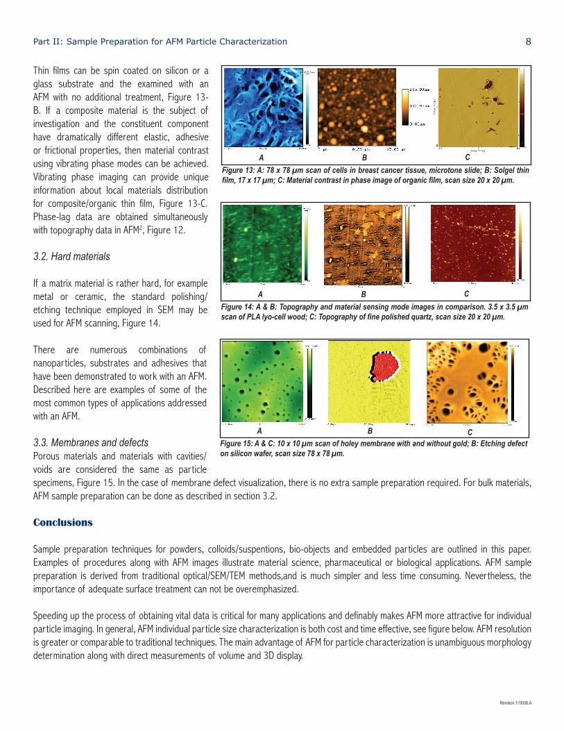
Thin films can be spin coated on silicon or a glass substrate and the examined with an AFM with no additional treatment, Figure 13-B. If a composite material is the subject of investigation and the constituent component have dramatically different elastic, adhesive or frictional properties, then material contrast using vibrating phase modes can be achieved. Vibrating phase imaging can provide unique information about local materials distribution for composite/organic thin film, Figure 13-C. Phase-lag data are obtained simultaneously with topography data in AFM2, Figure 12.

3.2. Hard materials

If a matrix material is rather hard, for example metal or ceramic, the standard polishing/etching technique employed in SEM may be used for AFM scanning, Figure 14.

There are numerous combinations of nanoparticles, substrates and adhesives that have been demonstrated to work with an AFM. Described here are examples of some of the most common types of applications addressed with an AFM.

3.3. Membranes and defectsPorous materials and materials with cavities/voids are considered the same as particle specimens, Figure 15. In the case of membrane defect visualization, there is no extra sample preparation required. For bulk materials, AFM sample preparation can be done as described in section 3.2.

Conclusions

Sample preparation techniques for powders, colloids/suspentions, bio-objects and embedded particles are outlined in this paper. Examples of procedures along with AFM images illustrate material science, pharmaceutical or biological applications. AFM sample preparation is derived from traditional optical/SEM/TEM methods,and is much simpler and less time consuming. Nevertheless, the importance of adequate surface treatment can not be overemphasized.

Speeding up the process of obtaining vital data is critical for many applications and definably makes AFM more attractive for individual particle imaging. In general, AFM individual particle size characterization is both cost and time effective, see figure below. AFM resolution is greater or comparable to traditional techniques. The main advantage of AFM for particle characterization is unambiguous morphology determination along with direct measurements of volume and 3D display.

Figure 14: A & B: Topography and material sensing mode images in comparison. 3.5 x 3.5 µm scan of PLA lyo-cell wood; C: Topography of fine polished quartz, scan size 20 x 20 µm.

A B C

Figure 15: A & C: 10 x 10 µm scan of holey membrane with and without gold; B: Etching defect on silicon wafer, scan size 78 x 78 µm.

A B C

Figure 13: A: 78 x 78 µm scan of cells in breast cancer tissue, microtone slide; B: Solgel thin film, 17 x 17 µm; C: Material contrast in phase image of organic film, scan size 20 x 20 µm.

A B C

Part II: Sample Preparation for AFM Particle Characterization 9

Revision.1/16/06.A

References:

1. G. Binning, C.F. Quate, Ch. Gerber, E. Weibel, Phys.Rev.Lett. 49, 57-61 (1982) 2. G. Binning, C.F. Quate and Ch. Gerber, Phys.Rev.Lett. 56, 930-933 (1986) 3. S. Dror, Scanning force microscopy: with applications to electric, magnetic and atomic forces, Oxford University Press, 1994 4. D.Bonnell, Scanning Probe Microscopy and spectroscopy, Wiley-VCH, 2001 5. B.P. Jena and J.K.H. Horber, Atomic force microscopy in cell biology, Academic Press, 2002 6. Zh. Peng and P. West, Appl.Phys.Lett. 86, 014107 (2005) 7. P. West, Zh.Peng, N.Starostina, American Laboratory, 23-24, april 2005 8. F. Stenley, Scanning and transmission electron microscopy, W.H.Freeman, 1993 9. P. Goodhew, J. Humpreys, R. Beanland, Electron microscopy and analysis, Taylor & Francis, 2001 10. D. Muller, M. Amrein, A. Engel, Jour.Struct.Biology 119,172-188 (1997) 11. V. Vadillo-Rodrigez, H. Busscher, W. Norde, J. Vries, R. Dijkstra, I. Stokroos and H. Mei, Applied and Enviromental Microbiolgy, 5441-5446, Sept.2004 12. K. Kirat, I. Burton, V. Dupres and Y. Duprene, Journal of Microscopy, 218,199-207 Pt3 (2005) 13. J. Vasenka, S. Manne, R. Gison, Th. Marsh, E. Henderson, Biophysical Journal 65, 992 (1993) 14. U. Swartz, H. Haefke, Th. Jung, E. Meyer, H-J Gunttherodt, Ultramicroscopy 41,435-439 (1992) 15. M. Van Cleef, S.Holt, G. Watson, S. Myhra, Journal of Microscopy, 181,2-9, Pt1 (1996) 16. C. Ritter, M. Heyde, U. Swartz, K. Rademann, Langmuir, 18,7798-7803, 2002 17. A. Engel and D. Muller, Nature Structural Biology 7, 715-718 (2000) 18. A. Morales, Ch.Lieber, Science, 279, 208-211 (1998) 19. P. Wagner, FEBS Letters 430, 112-115 (1998) 20. A. Bolshakova, O. Kiselyova, I. Yaminsky, Biotechnol.Prog 20,1615-1622 (2004) 21. H. Dai, Carbon Nanotubes, Topics Appl.Phys. 80, 29-53 (2001) 22. F. Moreno-Herrero, J. Colchero, J. Gomez-Herrero and A. Baro, Phys.Rev.E 69, 031915 (2004) 23. Tomaselli KJ, Damsky CH, Reichardt LF, J Cell Biol,105:2347 (1987) 24. A. McPherson, Yu. Kuznetsov, A. Malkin, M. Plomp, Jour.Struct.Biology, 142,32-46 (2003) 25. Yu. Kuznetsov, A. Low, H. Fan, A. McPherson, Virology, 323, 189-196, 2004 26. Yu. Kuznetsov, J. Gurnon, J. Van Etten, A. McPherson, Jour.Struct.Biology, 149, 256-263, 2005 27. P. West, N. Starostina, Advanced Materials & Processes, 35-37, February 2004

Advantages of using an AFM for particle analysis are:

• Faster than SEM and TEM • Instrumentation is more affordable • Direct three dimensional map • Works on many types of nanoparticles

Acknowledgments

The authors would like to thank Prof. P. Collins (UCI), Prof A. McPherson (UCI), Dr. Yu. Kuznetzov (UCI), Dr. M. Hines (Evidenttechnology, Inc.), and Dr. J. Baldeschwieler (CalTech) for fruitful discussions.