Part IB Inorganic Chemistry Option 1: Physical Methods in ...goodwin.chem.ox.ac.uk/goodwin/TEACHING_files/alg_ib_diffraction.pdf · Part IB Chemistry Option 1: Physical Methods in

$Page 1: Part IB Inorganic Chemistry Option 1: Physical Methods in ...goodwin.chem.ox.ac.uk/goodwin/TEACHING_files/alg_ib_diffraction.pdf · Part IB Chemistry Option 1: Physical Methods in$
Part IB Inorganic Chemistry

Option 1:Physical Methods in Inorganic ChemistryDiffraction Techniques

Dr Andrew L GoodwinHilary Term 2010

Seizure (detail), Roger Hiorns, 2009

Part IB ChemistryOption 1: Physical Methods in Inorganic Chemistry (Diffraction Techniques) 1

Lecture 1 (Monday 18/1/10): Reciprocal SpaceOverview of Physical Methods 1 course. Introduction to reciprocal space. Fourier relation-ship between real space and reciprocal space. Convolution and the convolution theorem.The reciprocal lattice.

Lecture 2 (Friday 22/1/10): Experimental TechniquesDiffraction geometry. Powder vs single-crystal diffraction. Neutron, x-ray and electrondiffraction. Thermal motion. Experimental data treatment.

Lecture 3 (Monday 25/1/10): Local StructurePatterson maps and the pair distribution function. Diffraction patterns of glasses, liquidsand amorphous materials. EXAFS.

Lecture 4 (Monday 8/3/10): Worked ExamplesIndexing non-cubic diffraction patterns. Structure factor calculations.

Standard texts on crystallography and diffraction

M. T. Dove, Structure and Dynamics (Oxford University Press, 2003).G. E. Bacon, Neutron Diffraction (Oxford University Press, 1975).G. Harburn, C. A. Taylor & T. R. Welberry, Atlas of optical transforms (Bell, 1975).M. F. C. Ladd & R. A. Palmer, Structure determination by X-ray crystallography (Plenum,1985).D. McKie & C. McKie, Essentials of Crystallography (Blackwell, 1986).P. Luger, Modern X-ray analysis on single crystals (de Gruyter, 1980).

Useful websites

You should also look at the course WWW pages, which contain links to a number of relevantsites—e.g. tutorials and other information:

http://goodwin.chem.ox.ac.uk/goodwin/TEACHING.html

A particularly useful website for learning about reciprocal space is the “Diffraction andFourier transform” Java applet written by Nicolas Schoeni and Gervais Chapuis:

http://escher.epfl.ch/eCrystallography/applets/fft.html

In addition, Kevin Cowtan has produced a very useful online “Book of Fourier”, from whichmany of the cat/duck examples used in this course are taken:

http://www.ysbl.york.ac.uk/∼cowtan/fourier/fourier.html

Some tips on indexing powder diffraction patterns (both cubic and non-cubic) are given onthe NCSU website:

http://wikis.lib.ncsu.edu/index.php/Powder diffraction/Indexing powder patterns


Three Spheres II, Maurits Escher, 1946

Lecture 1: Reciprocal space

Our goal in this course is to review the methods by which chemists have managed, overthe past century, to determine the atomic-level structure of materials. Much of this buildson your knowledge of crystallography and diffraction from Part IA, but we are going todeal with the concepts involved on a slightly deeper level. We will begin by revisiting thediffraction process itself, recasting our understanding in terms of “reciprocal space” — atopic that forms the subject of this first lecture.

In order to understand how diffraction really works, we need some idea of how wavesinteract with matter. And the key is to think of the arrangement of atoms in a material as aset of waves itself. A bizarre concept, perhaps. But actually atoms are small enough thatthe “particle-like” descriptions of structure we might instinctively seek to use — density ata given position in space — are no more real than the “wave-like” concepts of amplitudeand periodicity. It would seem strange, for example, to describe a wave on a body of waterin terms of a “mass”, or to locate it at a precise point in space. The same is true of theradiation one uses in a diffraction experiment, and in some senses the same is true evenof individual atoms. While our intuition lives in “real space”, where structure is a densityfunction ρ(r) that characterises how much matter is at a given point r, what we will developin this lecture is a feel for “reciprocal space”, where structure is defined instead in termsof a function F (Q) that tells us what components of waves of periodicity Q are required toproduce the same arrangement of atoms.


Let us first formalise what we mean by periodicity. Here there are two concepts: a waverepeats after a given distance, called the wavelength λ, and a wave propagates along aparticular direction. So by saying a wave has the periodicity Q we are defining Q = |Q| =2π/λ and assigning the direction Q/Q to be the same as the direction of propagation ofthe wave. Mathematically, we would represent the wave by the function ψ(r) = exp(iQ · r).Note that this function repeats every time that Q · r increases by another multiple of 2π,which will occur for each wavelength λ added to r in a direction parallel to Q. This is whatwe mean by a wave of wavelength λ that propagates parallel to Q.

A key point is that large values of Q correspond to waves with very small wavelengths,while small values of Q correspond to waves with long wavelengths. So, perhaps coun-terintuitively, as we add waves of larger and larger values of Q to assemble our materialstructure, we are actually making finer- and finer-scale adjustments in real space. Thebroadest features in real-space will be described by waves of smallest Q values in recip-rocal space. Note also that the units of Q are inverse length (usually A−1, since we will beusing A as units for structure on the atomic scale). So when we speak of reciprocal space,we are using inverse lengths as our units.

The conversion itself between real space and reciprocal space is relatively straightforward.As we said above, our reciprocal space function F (Q) is meant to tell us what componentsof waves of periodicity Q are needed to produce the real-space density function ρ(r). Thisis precisely the mapping described by Fourier transforms, which tell us how to deconstructany function into an equivalent set of waves of different periodicities. The mathematicsgives us then:

F (Q) =

∫ρ(r) exp(iQ · r) dr, (1)

ρ(r) =1

2π

∫F (Q) exp(−iQ · r) dQ. (2)

We will see in the next lecture that what diffraction does is to give us a way of measuringF (Q) (or, at least, related functions). In principle, if we measure F (Q) for sufficientlymany values of Q then we could use the reverse Fourier transform (equation (2) above)to reconstruct the distribution function ρ(r). This is the underlying idea of crystallography.There are problems along the way, and we will deal with these as we come to them. But forthe time being what is most important is for us to develop an intuition for what F (Q) lookslike for different systems — how it is related to ρ(r) and what it can tell us in itself aboutmaterial structure.

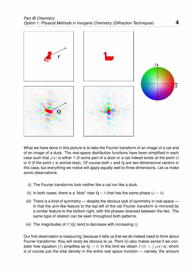
Perhaps the first thing to note about F (Q) is that it is a complex number (even giventhat the real-space distribution ρ(r) is real, and positive, everywhere). As such, we canthink separately about its magnitude |F (Q)| and its complex argument φ, which we callits “phase”; that is, F (Q) = |F (Q)| × exp(iφ). We will use a very convenient method ofrepresenting both of these components pictorially (see following figure), where a diagramof reciprocal space is coloured such that the intensity at a given point Q corresponds tothe magnitude of F (Q), and the colour tells us about the phase φ.


What we have done in this picture is to take the Fourier transform of an image of a cat andof an image of a duck. The real-space distribution functions have been simplified in eachcase such that ρ(r) is either 1 (if some part of a duck or a cat indeed exists at the point r)or 0 (if the point r is animal-less). Of course both r and Q are two-dimensional vectors inthis case, but everything we notice will apply equally well to three dimensions. Let us makesome observations:

(i) The Fourier transforms look neither like a cat nor like a duck.

(ii) In both cases, there is a “blob” near Q = 0 that has the same phase (φ ∼ 0).

(iii) There is a kind of symmetry — despite the obvious lack of symmetry in real-space —in that the arm-like feature to the top-left of the cat Fourier transform is mirrored bya similar feature to the bottom-right, with the phases reversed between the two. Thesame type of relation can be seen throughout both patterns.

(iv) The magnitudes of F (Q) tend to decrease with increasing Q.

Our first observation is reassuring, because it tells us that we do indeed need to think aboutFourier transforms: they will rarely be obvious to us. Point (ii) also makes sense if we con-sider how equation (1) simpilfies as Q → 0: in this limit we obtain F (0) =

∫ρ(r) dr, which

is of course just the total density in the entire real space function — namely, the amount


of cat or the amount of duck. Since both are positive and real, we expect a positive andreal value for F (0); hence the graphical Fourier transforms are intense and red-coloured attheir centres. Our statement with regard to symmetry also follows from equation (1) if weconsider the relationship between F (Q) and F (−Q):

F (−Q) =

∫ρ(r) exp(−ir ·Q) dr =

[∫ρ(r) exp(iQ · r) dr

]∗= [F(Q)]∗, (3)

where the asterisk notation represents the operation of complex conjugation. Hence themagnitudes of F (Q) and F (−Q) are identical, and their phases reversed. This rule isknown as “Friedel’s law”, which also demands that F (0) must be real.

To understand the last of our four observations, we must recall our statements above con-cerning the meaning of F (Q) at large Q. The bulk of the density in real space — the factthat, for either cat or duck, we basically have a collection of density near the origin andnot much else — will be recovered from the long-wavelength information near Q = 0. Thehigh-frequency information at larger Q will help separate the cat’s tail from its body, or willgive the duck its beak and wings. This sort of detail concerns less and less density in realspace, and so the components of the waves required will decrease with increasing Q.

In the picture above we have illustrated this by calculating the reverse Fourier transform ofthe duck image with different parts of reciprocal space excluded. If we use just the low Q

region (left hand side in the image above), then we get the broad features of the duck; if weuse just the high Q region, then we obtain the edges. Indeed these approaches are usedin image processing for compression (low Q filtering) or to determine edges (high Q).

A useful mathematical concept when dealing with Fourier transforms is called convolutionand is a little strange. It is the idea of combining two functions such that we place a copy


of one function at each point in space, weighted by the value of the second function atthe same point. The mathematics is dealt with separately in an appendix, but the concept(which is all that is important) is explained more satisfactorily through a diagram.

On the left hand side we have two density functions: the first might reasonably represent asingle molecule, while the second is just a set of points. What the convolution of these twofunctions does is to place a copy of the molecule at each point in the set (or, equivalently,to copy the set of points for each atom in the molecule). We end up with a set of molecules,whose spacing is determined by the original set of points. The convolution operation itselfis represented by the operator ⊗, and is quite useful because it enables us to deconstructa complex object (a group of molecules) into two simpler objects: a single molecule andan array of points. But it is even more useful in the current context, because the Fouriertransform of a convolution is equivalent to the product of the individual Fourier transforms.Let us see this pictorially in terms of the Fourier transforms of the above images:

Note that the Fourier transform of the grid of points is itself real-valued everywhere, so thatthe phases in the final result come directly from the phases for the individual molecule.So on the one hand the phases are telling us something about the molecule, while on theother hand the grid-like pattern is telling us about how the molecules are repeated in realspace.

Of course, the essential feature that distinguishes the crystalline form as a state of matteris the existence, on the atomic scale, of some recurring structural unit — be it a single atomor a group of atoms — whose repeat extends at regular intervals in all three dimensions.As we know, the crystal is built up from from a tessellation of these identical unit cells, suchthat the contents of any one unit cell can be mapped directly onto the contents of anotherthrough translations alone.


Here is where the concept of convolution is so useful: it enables us to consider an entirecrystal lattice as the contents of a single unit cell (the “motif”) convoluted with a lattice ofpoints that describes the tessellation itself — how the unit cells are stacked together toform the crystal. In order to understand the Fourier transform of a crystal, all we need isto understand the Fourier transform of the motif and the Fourier transform of the lattice ofpoints. We can take the product of these two transforms to arrive at the Fourier transformof the crystal itself.

So the question now is to ask what the Fourier transform of a lattice actually looks like.To answer this, let us first define the lattice mathematically as a series of delta-functionslocated at integral combinations of the unit cell vectors a, b and c:

L(r) =∑UVW

δ[r− (Ua + V b +Wc)]. (4)

We could do the mathematics (and indeed all is written out in gory detail in an appendix),and calculate the Fourier transform R(Q) =

∫ ∑UVW δ[r− (Ua + V b +Wc)] exp(iQ · r) dr

directly. The result is a lattice itself, now running throughout reciprocal space:

R(Q) =∑hkl

δ[Q− (ha∗ + kb∗ + lc∗)]. (5)

Here the “reciprocal lattice vectors” a∗, b∗ and c∗ generate this “reciprocal lattice”:

a∗ = 2πb× c

a · (b× c), b∗ = 2π

c× a

b · (c× a), c∗ = 2π

a× b

c · (a× b). (6)

These equations look more complicated than they actually are. Their derivation is givenas an appendix, but we are really only concerned with their meaning (the important thing,after all). In each case, the cross product contained in the numerator produces a vectorthat is perpendicular to the two real-space axes involved. That is, b × c — and hencea∗ — is perpendicular to b and c. In cases where a, b and c are not orthogonal (suchas in hexagonal systems), then a∗ may not necessarily be parallel to a, and so on. Thedenominator is actually the same value in each case: namely, the unit cell volume. It scalesthe vector to the correct length, and it’s not too hard to see that in simple systems we endup with intuitive results.


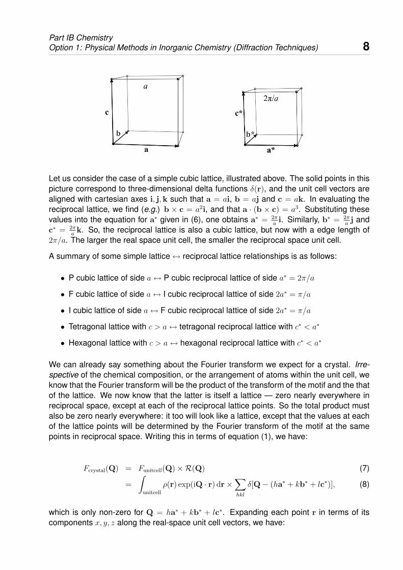
Let us consider the case of a simple cubic lattice, illustrated above. The solid points in thispicture correspond to three-dimensional delta functions δ(r), and the unit cell vectors arealigned with cartesian axes i, j,k such that a = ai, b = aj and c = ak. In evaluating thereciprocal lattice, we find (e.g.) b × c = a2i, and that a · (b × c) = a3. Substituting thesevalues into the equation for a∗ given in (6), one obtains a∗ = 2π

ai. Similarly, b∗ = 2π

aj and

c∗ = 2πak. So, the reciprocal lattice is also a cubic lattice, but now with a edge length of

2π/a. The larger the real space unit cell, the smaller the reciprocal space unit cell.

A summary of some simple lattice↔ reciprocal lattice relationships is as follows:

• P cubic lattice of side a↔ P cubic reciprocal lattice of side a∗ = 2π/a

• F cubic lattice of side a↔ I cubic reciprocal lattice of side 2a∗ = π/a

• I cubic lattice of side a↔ F cubic reciprocal lattice of side 2a∗ = π/a

• Tetragonal lattice with c > a↔ tetragonal reciprocal lattice with c∗ < a∗

• Hexagonal lattice with c > a↔ hexagonal reciprocal lattice with c∗ < a∗

We can already say something about the Fourier transform we expect for a crystal. Irre-spective of the chemical composition, or the arrangement of atoms within the unit cell, weknow that the Fourier transform will be the product of the transform of the motif and the thatof the lattice. We now know that the latter is itself a lattice — zero nearly everywhere inreciprocal space, except at each of the reciprocal lattice points. So the total product mustalso be zero nearly everywhere: it too will look like a lattice, except that the values at eachof the lattice points will be determined by the Fourier transform of the motif at the samepoints in reciprocal space. Writing this in terms of equation (1), we have:

Fcrystal(Q) = Funitcell(Q)×R(Q) (7)

=

∫unitcell

ρ(r) exp(iQ · r) dr×∑hkl

δ[Q− (ha∗ + kb∗ + lc∗)], (8)

which is only non-zero for Q = ha∗ + kb∗ + lc∗. Expanding each point r in terms of itscomponents x, y, z along the real-space unit cell vectors, we have:


Fcrystal(hkl) =

∫unitcell

ρ(r) exp[i(ha∗ + kb∗ + lc∗) · (xa + yb + zc)] dr (9)

=

∫unitcell

ρ(r) exp[2πi(hx+ ky + lz)] dr. (10)

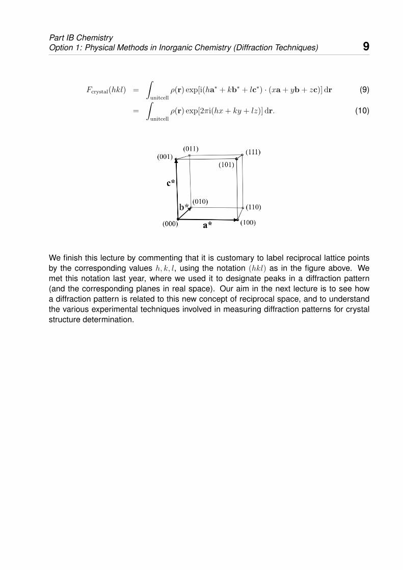
We finish this lecture by commenting that it is customary to label reciprocal lattice pointsby the corresponding values h, k, l, using the notation (hkl) as in the figure above. Wemet this notation last year, where we used it to designate peaks in a diffraction pattern(and the corresponding planes in real space). Our aim in the next lecture is to see howa diffraction pattern is related to this new concept of reciprocal space, and to understandthe various experimental techniques involved in measuring diffraction patterns for crystalstructure determination.


1024 Farben, Gerhard Richter, 1973

Lecture 2: Experimental Techniques

We have now seen, in the first lecture, how material structure can be thought of in termsof reciprocal space — a bizarre world where the arrangement of atoms is built up froma superposition of different waves. Reciprocal space is actually quite a central conceptin much of solid state chemistry and condensed matter physics, so it is a concept worthunderstanding in itself. But its particular relevance in a crystallographic context is that it isa reciprocal-space view of material structure that one obtains in a diffraction experiment.When we shine a suitable beam of radiation at a crystal, the beam diffracts, and the patternof spots we see is actually a direct view of the reciprocal lattice we learned about in Lecture1. Our first goal in this lecture is to explain how the reciprocal space formalisms we havedeveloped are consistent with the Bragg equations we studied in Part IA.

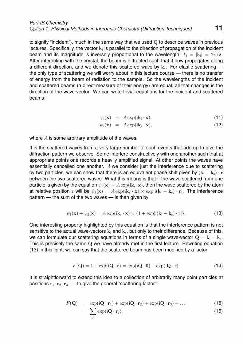
The diffraction process begins with a beam of radiation, which we consider to be a wavepropagating through space. The types of radiation usually used are x-rays or neutrons,and we will cover these in greater depth shortly. For the time being, the important conceptis that this radiation is a wave and, as such, can be described by a wave-vector ki (“i” here


to signify “incident”), much in the same way that we used Q to describe waves in previouslectures. Specifically, the vector ki is parallel to the direction of propagation of the incidentbeam and its magnitude is inversely proportional to the wavelength: ki = |ki| = 2π/λ.After interacting with the crystal, the beam is diffracted such that it now propagates alonga different direction, and we denote this scattered wave by ks. For elastic scattering —the only type of scattering we will worry about in this lecture course — there is no transferof energy from the beam of radiation to the sample. So the wavelengths of the incidentand scattered beams (a direct measure of their energy) are equal; all that changes is thedirection of the wave-vector. We can write trivial equations for the incident and scatteredbeams:

ψi(x) = A exp(iki · x), (11)ψs(x) = A exp(iks · x), (12)

where A is some arbitrary amplitude of the waves.

It is the scattered waves from a very large number of such events that add up to give thediffraction pattern we observe. Some interfere constructively with one another such that atappropriate points one records a heavily amplified signal. At other points the waves haveessentially cancelled one another. If we consider just the interference due to scatteringby two particles, we can show that there is an equivalent phase shift given by (ki − ks) · rbetween the two scattered waves. What this means is that if the wave scattered from oneparticle is given by the equation ψ1(x) = A exp(iks ·x), then the wave scattered by the atomat relative position r will be ψ2(x) = A exp(iks · x) × exp[i(ki − ks) · r]. The interferencepattern — the sum of the two waves — is then given by

ψ1(x) + ψ2(x) = A exp(iks · x)× {1 + exp[i(ki − ks) · r]}. (13)

One interesting property highlighted by this equation is that the interference pattern is notsensitive to the actual wave-vectors ki and ks, but only to their difference. Because of this,we can formulate our scattering equations in terms of a single wave-vector Q = ki − ks.This is precisely the same Q we have already met in the first lecture. Rewriting equation(13) in this light, we can say that the scattered beam has been modified by a factor

F (Q) = 1 + exp(iQ · r) = exp(iQ · 0) + exp(iQ · r). (14)

It is straightforward to extend this idea to a collection of arbitrarily many point particles atpositions r1, r2, r3, . . . to give the general “scattering factor”:

F (Q) = exp(iQ · r1) + exp(iQ · r2) + exp(iQ · r3) + . . . (15)

=∑j

exp(iQ · rj). (16)


Indeed, by converting this sum to an integral over all space we allow a further generalisa-tion to arbitrary particle distributions (i.e. allowing for non-point particles):

F (Q) =

∫ρ(r) exp(iQ · r) dr. (17)

This equation should be entirely familiar. What we have shown here is quite remarkable:namely, that the scattering process is nothing but a Fourier transformation itself. In adiffraction experiment, the scattered wave characterised by ks tells us about the Fouriercomponent at the wave-vector Q = ki−ks. By measuring the scattered waves for differentwave-vectors ks (and, effectively, for different Q), we can actually piece together a picture ofreciprocal space. Diffraction is an experimental technique that allows us to view reciprocalspace directly.

Well, almost. There is (as always) one fundamental problem. Namely, that when we detecta scattered wave such as F (Q), what we are measuring is not the wave itself, but someintensity I(Q) that is proportional to the square of its modulus: I(Q) ∝ |F (Q)|2. Thisintensity is a real positive value, whereas the amplitude F (Q) is a complex number. Bymeasuring intensity rather than amplitude we have surrendered all information about thephase of the amplitude. In terms of our cat/duck Fourier transform illustrations of the lastlecture, what we are saying is that we measure the intensity of the colours in the Fourierimages, but not the colours themselves. This makes it very difficult to reconstruct a real-space description of structure from what is an incomplete “colour-blind” reciprocal-spacedescription. Known as the “phase problem”, this issue is a real hurdle for crystallography.There are good clues from crystal symmetry and some clever maths comes in handy too.We will not have the chance in this short course to cover the details of how the phaseproblem is overcome, but it is important at this stage to know at least that it exists and whyit is indeed a problem.

For the time being, we will concern ourselves a little more with the geometry of diffractionexperiments, and the relationship between the various quantities involved. The first thingwe will do is to relate our scattering vector Q to the various diffraction concepts we firstencountered in second year: namely, the Bragg diffraction angle 2θ, d-spacing and theBragg law. Reminding ourselves of the scattering geometry illustrated in the diagram onpage 10, we begin with the relationship

Q2 = |Q|2 = |ki − ks|2 = k2i + k2

s (18)= k2

i + k2s − 2kiks cos 2θ (19)

= 2

(2π

λ

)2

− 2

(2π

λ

)2

cos 2θ (20)

=16π2

λ2sin2 θ, (21)


where we have used the identity 1 − cos 2θ = 2 sin2 θ. Consequently, the magnitude Q ofthe scattering vector is related to the Bragg angle θ by the equation

Q =4π

λsin θ. (22)

Bragg’s law told us that we expect to see a diffraction peak corresponding to the Braggangle θ whenever there were a set of atomic planes separated by the distance d = λ/2 sin θ.Recasting this in terms of Q, we have

Q =2π

d. (23)

Hopefully this should make complete sense in terms of our picture of the reciprocal lattice.We now know, from Lecture 1, that we expect only to see components in reciprocal spacewhenever Q is a reciprocal lattice vector Q = ha∗ + kb∗ + lc∗. The corresponding magni-tude of Q is quite easy to calculate in the case where the lattice (and reciprocal lattice) isorthogonal: by Pythagoras we have

Q =[(ha∗)2 + (kb∗)2 + (lc∗)2

]1/2 (24)

=

[4π2h2

a2+

4π2k2

b2+

4π2l2

c2

]1/2

, (25)

which, when substituted into equation (23) gives us the (hopefully) familiar expression ford-spacing in an orthogonal crystal:

1

d2=h2

a2+k2

b2+l2

c2. (26)

In a powder diffraction experiment we see a one-dimensional representation of reciprocalspace: it is as if the reciprocal lattice has been collapsed onto a single axis, with the origin(000) at the left-hand side of a diffractogram and intensities then measured as a function


of the increasing magnitudes Q. Nevertheless we can still think of each peak as belongingto a specific point in the full three-dimensional reciprocal lattice. One useful exercise is toconsider what happens to the reciprocal lattice and its corresponding powder diffractionpattern as a cubic crystal is elongated slightly along one of its three axes.

Both powder and single-crystal diffraction experiments have advantages and disadvan-tages, and the preference for one or the other relies on a number of factors, including:

(i) Single crystals can often be difficult to grow of a sufficient size (∼mm3) — especiallyfor neutron experiments, where cm−3 samples are needed. In such cases, powderdiffraction may be the only plausible crystallographic technique available. Sometimesa sample that appears to consist of single crystals is actually highly “twinned” — thatis, where each block actually consists of a number of domains related to varyingdegrees by different symmetries.

(ii) Naturally, single-crystal diffraction patterns give three-dimensional representations ofreciprocal space, whereas this information is collapsed onto a single axis for powderdiffraction experiments. There is a loss of information involved in the powder aver-aging process, and consequently structure solution is much more difficult in generalfrom powder data than from single crystal data.

(iii) In general, the best single crystal diffractometers have a lower reciprocal-space res-olution than the best powder diffractometers. This means that subtle structural dis-tortions can often be missed in single crystal experiments, but become evident inpowder data. For this reason, powder diffraction is very often the method of choicefor monitoring the structural changes associated with phase transitions in crystallinematerials.

(iv) Powder diffraction experiments can be complicated by “preferred orientation” — wherebythe crystallites in the powder do not pack entirely randomly, and this leads to changesin the observed reflection intensities. This problem is often most noticeable for highlyanisotropic systems, e.g. with rod-like or layered structures.

(v) Single crystal experiments are of limited use in assessing the purity of a chemicalsample, since the experiment is only performed on a small and specifically-chosensubset of the actual sample. Powder diffraction allows the chemist to determine thenumber and proportions of different phases present because even a small samplecan be representative of the whole.

Irrespective of whether we are studying powders or single crystals, there is a physicallimitation on the maximum value of 2θ that one can measure: namely, 2θ = 180◦. Thismeans that we can only measure reciprocal space up to a maximum value Qmax = 4π/λ

(by equation (22)). The use of shorter wavelengths λ would enable us to measure more ofreciprocal space, but we will never be able to measure everything. The physical meaning ofthis minimum wavelength is that it corresponds to the finest level of detail in real space thatone can hope to resolve from a reverse Fourier transform of the diffraction data. We have


already seen that the exclusion of high frequency components in our Fourier duck (page 5)meant that we could not distinguish either its beak or its wings. So, if we are to distinguishneighbouring atoms from one another, we will need a sufficiently small wavelength to givea real-space resolution of about 1 A.

There are two principal types of radiation that satisfy this requirement. The first is a beamof x-rays, and the second is a beam of thermal neutrons. There are many similaritiesbetween these two sources of radiation — certainly they both produce diffraction patternsas described above. But there are a number of important differences, due primarily to thedifferent physics associated with their scattering mechanisms. The overall message is thatwe can obtain complementary information from x-ray diffraction and neutron diffraction:much of the cutting-edge science in the field exploits features of both techniques.

X-rays are the part of the electromagnetic spectrum with wavelengths in the range 0.1–100 A, and hence with energies in the range 102–105 eV. To appreciate this energy scale,we note that the kinetic energy of an atom in a gas at room temperature is 0.025 eV. Indeed,x-rays are sufficiently energetic to ionise atoms, and can interfere with the chemistry ofmaterials over even quite short periods.

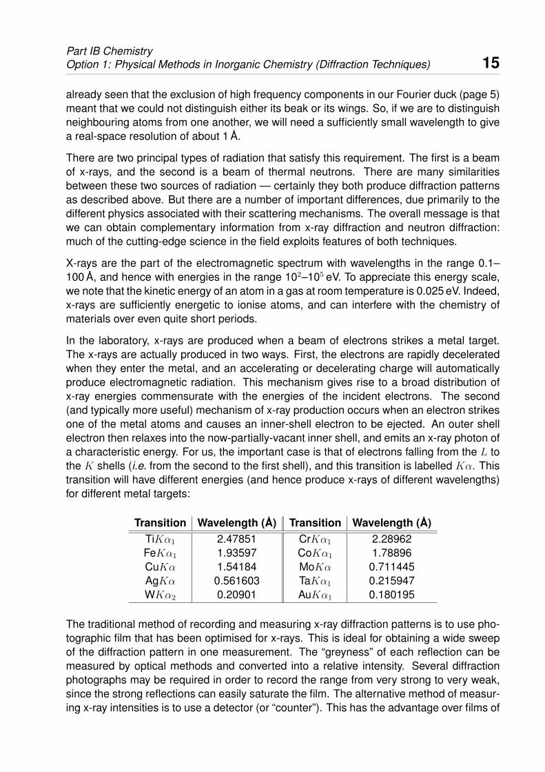
In the laboratory, x-rays are produced when a beam of electrons strikes a metal target.The x-rays are actually produced in two ways. First, the electrons are rapidly deceleratedwhen they enter the metal, and an accelerating or decelerating charge will automaticallyproduce electromagnetic radiation. This mechanism gives rise to a broad distribution ofx-ray energies commensurate with the energies of the incident electrons. The second(and typically more useful) mechanism of x-ray production occurs when an electron strikesone of the metal atoms and causes an inner-shell electron to be ejected. An outer shellelectron then relaxes into the now-partially-vacant inner shell, and emits an x-ray photon ofa characteristic energy. For us, the important case is that of electrons falling from the L tothe K shells (i.e. from the second to the first shell), and this transition is labelled Kα. Thistransition will have different energies (and hence produce x-rays of different wavelengths)for different metal targets:

Transition Wavelength (A) Transition Wavelength (A)TiKα1 2.47851 CrKα1 2.28962FeKα1 1.93597 CoKα1 1.78896CuKα 1.54184 MoKα 0.711445AgKα 0.561603 TaKα1 0.215947WKα2 0.20901 AuKα1 0.180195

The traditional method of recording and measuring x-ray diffraction patterns is to use pho-tographic film that has been optimised for x-rays. This is ideal for obtaining a wide sweepof the diffraction pattern in one measurement. The “greyness” of each reflection can bemeasured by optical methods and converted into a relative intensity. Several diffractionphotographs may be required in order to record the range from very strong to very weak,since the strong reflections can easily saturate the film. The alternative method of measur-ing x-ray intensities is to use a detector (or “counter”). This has the advantage over films of


giving the intensity directly and more accurately. The disadvantage is that a single detectorwill only record a single point in reciprocal space at any one time. This problem can beovercome by using area detectors that contain a large number of pixels, each of which iscapable of recording its own signal. These are now the most widely used form of detector.

One fundamental limitation on the use of x-ray tubes is that the maximum intensity is limitedby the need to prevent overheating of the target. X-ray production is not very efficient, andmost of the energy of the incident electron beam is lost as heat. This can be overcome inpart by using rotating targets, so that the electron beam does not strike a single area of thetarget. However, there is still a mechanical limitation on the maximum intensity produced.Moreover, the wavelength of x-rays produced by a given x-ray tube is determined by thenature of its metal target, and so is not variable.

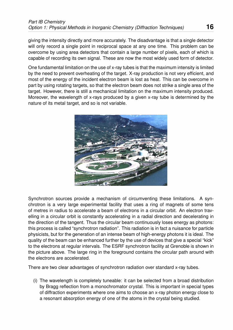
Synchrotron sources provide a mechanism of circumventing these limitations. A syn-chrotron is a very large experimental facility that uses a ring of magnets of some tensof metres in radius to accelerate a beam of electrons in a circular orbit. An electron trav-elling in a circular orbit is constantly accelerating in a radial direction and decelerating inthe direction of the tangent. Thus the circular beam continuously loses energy as photons:this process is called “synchrotron radiation”. This radiation is in fact a nuisance for particlephysicists, but for the generation of an intense beam of high-energy photons it is ideal. Thequality of the beam can be enhanced further by the use of devices that give a special “kick”to the electrons at regular intervals. The ESRF synchrotron facility at Grenoble is shown inthe picture above. The large ring in the foreground contains the circular path around withthe electrons are accelerated.

There are two clear advantages of synchrotron radiation over standard x-ray tubes.

(i) The wavelength is completely tuneable: it can be selected from a broad distributionby Bragg reflection from a monochromator crystal. This is important in special typesof diffraction experiments where one aims to choose an x-ray photon energy close toa resonant absorption energy of one of the atoms in the crystal being studied.


(ii) The intensity is increased by many orders of magnitude. This permits the use ofsmaller crystals, increases the resolution of the observed diffraction patterns andallows incredibly fast measurements so that kinetic studies can be performed.

The second type of radiation, namely a beam of thermal neutrons, can be produced in oneof two ways. The “traditional” method is to generate beams of neutrons within a nuclearreactor. These are produced in the form of a broad spectrum. Individual wavelengthscan be selected by Bragg diffraction from a crystal monochromator (as for x-rays). Inthis situation the diffraction equipment that utilises the neutron beam is similar in principleto that used with laboratory x-ray beams. The primary difference is one of scale: theneutron apparatus is typically much larger. In addition to scale, there is a key environmentalproblem in this method of producing neutrons, perhaps unsurprisingly, requires a nuclearreactor

A modern alternative source of neutrons — the second method of generating thermalneutrons alluded to above — is called a “spallation source”. At such a facility, the productionof neutrons begins when a beam of high-energy protons is fired into a heavy-metal target(such as tungsten). The protons strike the nuclei and eject high-energy neutrons. In factthe energies of these neutrons are too high to be useful, so they are slowed down bya moderating material (e.g. liquid methane). The moderator acts to absorb much of theneutrons’ energy, producing a spectrum of neutrons with useable wavelengths. Differentmoderators produce slightly different distributions of wavelengths, and this property can beexploited for various applications.

The initial beam of protons is pulsed, so the beam of neutrons is also produced in a se-ries of discrete pulses. The neutron scattering instrumentation at a spallation source ex-ploits the pulsed nature of the neutron beam by measuring the wavelength by time-of-flighttechniques. This avoids the wastage incurred by selecting individual wavelengths with a


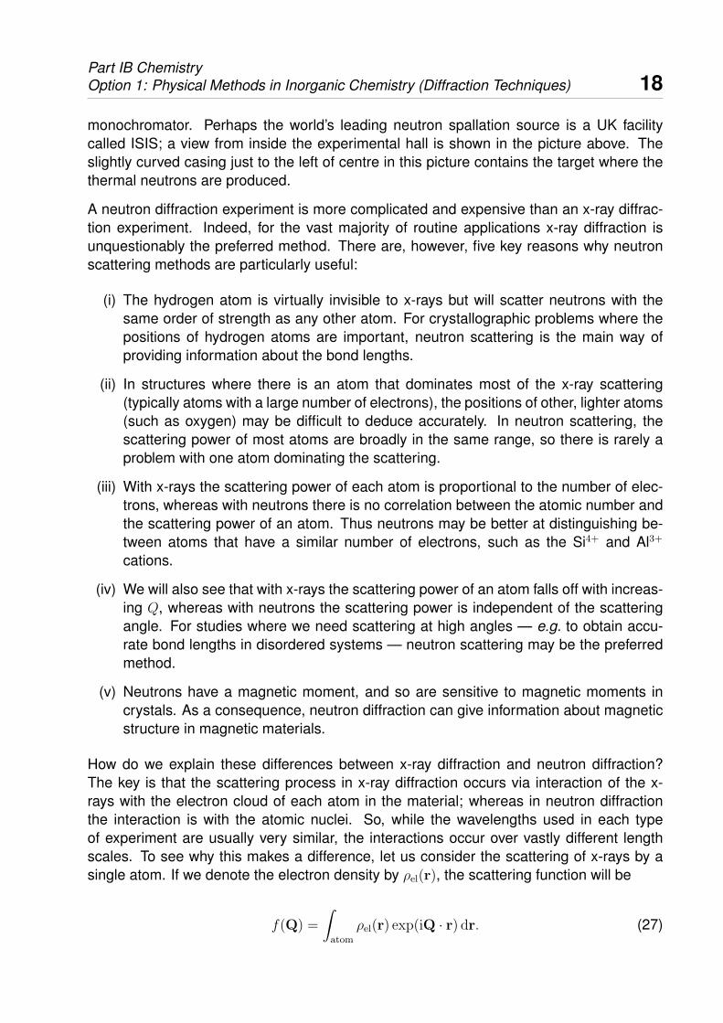
monochromator. Perhaps the world’s leading neutron spallation source is a UK facilitycalled ISIS; a view from inside the experimental hall is shown in the picture above. Theslightly curved casing just to the left of centre in this picture contains the target where thethermal neutrons are produced.

A neutron diffraction experiment is more complicated and expensive than an x-ray diffrac-tion experiment. Indeed, for the vast majority of routine applications x-ray diffraction isunquestionably the preferred method. There are, however, five key reasons why neutronscattering methods are particularly useful:

(i) The hydrogen atom is virtually invisible to x-rays but will scatter neutrons with thesame order of strength as any other atom. For crystallographic problems where thepositions of hydrogen atoms are important, neutron scattering is the main way ofproviding information about the bond lengths.

(ii) In structures where there is an atom that dominates most of the x-ray scattering(typically atoms with a large number of electrons), the positions of other, lighter atoms(such as oxygen) may be difficult to deduce accurately. In neutron scattering, thescattering power of most atoms are broadly in the same range, so there is rarely aproblem with one atom dominating the scattering.

(iii) With x-rays the scattering power of each atom is proportional to the number of elec-trons, whereas with neutrons there is no correlation between the atomic number andthe scattering power of an atom. Thus neutrons may be better at distinguishing be-tween atoms that have a similar number of electrons, such as the Si4+ and Al3+

cations.

(iv) We will also see that with x-rays the scattering power of an atom falls off with increas-ing Q, whereas with neutrons the scattering power is independent of the scatteringangle. For studies where we need scattering at high angles — e.g. to obtain accu-rate bond lengths in disordered systems — neutron scattering may be the preferredmethod.

(v) Neutrons have a magnetic moment, and so are sensitive to magnetic moments incrystals. As a consequence, neutron diffraction can give information about magneticstructure in magnetic materials.

How do we explain these differences between x-ray diffraction and neutron diffraction?The key is that the scattering process in x-ray diffraction occurs via interaction of the x-rays with the electron cloud of each atom in the material; whereas in neutron diffractionthe interaction is with the atomic nuclei. So, while the wavelengths used in each typeof experiment are usually very similar, the interactions occur over vastly different lengthscales. To see why this makes a difference, let us consider the scattering of x-rays by asingle atom. If we denote the electron density by ρel(r), the scattering function will be

f(Q) =

∫atom

ρel(r) exp(iQ · r) dr. (27)


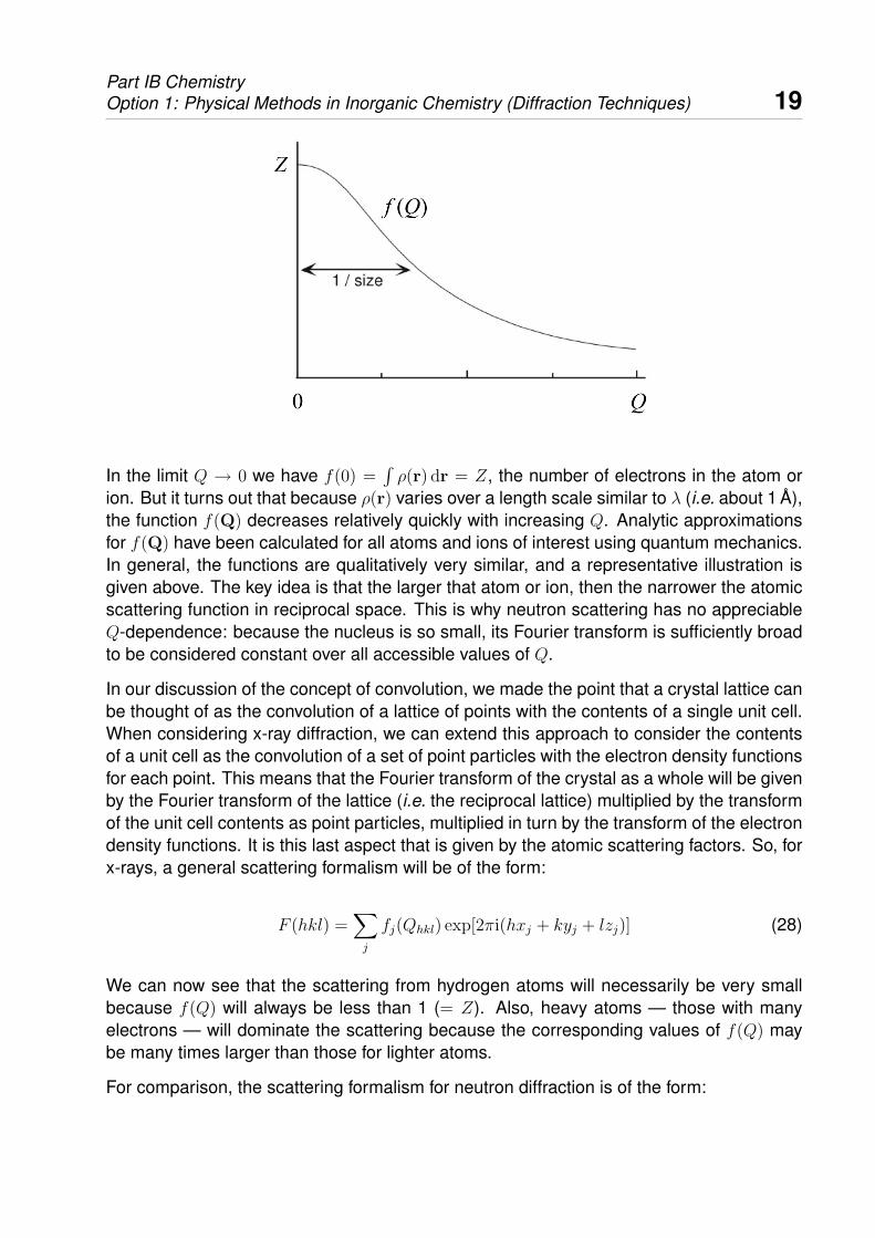
In the limit Q → 0 we have f(0) =∫ρ(r) dr = Z, the number of electrons in the atom or

ion. But it turns out that because ρ(r) varies over a length scale similar to λ (i.e. about 1 A),the function f(Q) decreases relatively quickly with increasing Q. Analytic approximationsfor f(Q) have been calculated for all atoms and ions of interest using quantum mechanics.In general, the functions are qualitatively very similar, and a representative illustration isgiven above. The key idea is that the larger that atom or ion, then the narrower the atomicscattering function in reciprocal space. This is why neutron scattering has no appreciableQ-dependence: because the nucleus is so small, its Fourier transform is sufficiently broadto be considered constant over all accessible values of Q.

In our discussion of the concept of convolution, we made the point that a crystal lattice canbe thought of as the convolution of a lattice of points with the contents of a single unit cell.When considering x-ray diffraction, we can extend this approach to consider the contentsof a unit cell as the convolution of a set of point particles with the electron density functionsfor each point. This means that the Fourier transform of the crystal as a whole will be givenby the Fourier transform of the lattice (i.e. the reciprocal lattice) multiplied by the transformof the unit cell contents as point particles, multiplied in turn by the transform of the electrondensity functions. It is this last aspect that is given by the atomic scattering factors. So, forx-rays, a general scattering formalism will be of the form:

F (hkl) =∑j

fj(Qhkl) exp[2πi(hxj + kyj + lzj)] (28)

We can now see that the scattering from hydrogen atoms will necessarily be very smallbecause f(Q) will always be less than 1 (= Z). Also, heavy atoms — those with manyelectrons — will dominate the scattering because the corresponding values of f(Q) maybe many times larger than those for lighter atoms.

For comparison, the scattering formalism for neutron diffraction is of the form:


F (hkl) =∑j

bj exp[2πi(hxj + kyj + lzj)], (29)

where bj is the “neutron scattering length” for the atom j — a quantity that describes howstrongly that particular type of atom scatters neutrons. There is no systematic variation inthe scattering lengths as a function of atomic size, and both positive and negative valuesare known; consequently, similarly sized atoms can actually scatter neutrons quite differ-ently. This means that x-ray and neutron diffraction experiments emphasise different typesof atoms differently, and this can be of enormous help in separating the scattering due toindividual types of atoms, such as hydrogen.

Electron diffraction is a third diffraction technique, where the scattering process now in-volves a beam of high-energy electrons — usually generated in a transmission electronmicroscope (TEM). The wavelength involved is very small (λ ' 0.01–0.1 A), so in principleone can see quite a lot of reciprocal space. The electron beam also has a high intensity,and this gives rise to two effects: on the one hand, it means that the technique is verywell suited to observing weak diffraction features, such as superlattice peaks or structureddiffuse scattering; on the other hand, it means also that is highly destructive, and materialsmay only survive under an electron beam for seconds (or less). Because electrons reactwith materials so very easily, it is necessary to use very thin samples, and to illuminate onlya very small cross-section (typically 10–100 nm). This has the advantage, however, thatsingle-crystal-like patterns can be obtained from microcrystalline powder samples. Finally,electron diffraction obeys essentially the same scattering equations as for x-rays, since thescattering process involves deflection by the electron clouds of individual atoms.

For completeness, we will consider one other contribution to the scattering functions that isrelevant to both neutron and x-ray diffraction patterns. That is the effect of thermal motion,which essentially acts to blur the position of each atom. To account for this, the positionof each atom needs to be convoluted with the spread of displacements that arise fromthe thermal motion. Consequently, the Fourier transform of the unit cell incorporates theFourier transform of the spread of displacements as an additional multiplicative factor. Ifwe assume that the thermal motion is isotropic and harmonic, then the Fourier transformof the spread of displacements (which for harmonic motion will be a Gaussian distribution)is given as

Tj(Q) = exp(−8π2〈u2j〉 sin2 θ/λ2) (30)

= exp(−Bj sin2 θ/λ2), (31)

where 〈u2j〉 is the mean-squared displacement of atom j, and Bj is commonly-used short-

hand for the quantity 8π2〈u2j〉. Because 〈u2

j〉 is found to be proportional to temperature(except at low temperatures), this is usually called the “temperature factor”, An alternativename is the “Debye-Waller factor”, after the people who first developed the theory. So,taking into consideration the thermal motion, the x-ray structure factor becomes


F (hkl) =∑j

f(Qhkl) exp[2πi(hxj + kyj + lzj)] exp(−Bj sin2 θhkl/λ2). (32)

The primary effect of thermal motion on the diffraction pattern is to reduce the intensities ofthose reflections at large Q (large θ). As temperature increases, the displacement param-eters Bj will increase, and the corresponding exponential term in equation (32) decreases,reducing the intensities further.


Wall Drawing 1186 (detail), Sol Lewitt, 2005

Lecture 3: Local Structure

We begin this lecture by returning to the idea that a diffraction experiment measures somequantity proportional to the square of the modulus of the structure factor; i.e., I(Q) ∝|F (Q)|2. Despite the fact that we have lost much of the information contained within F (Q),there is still merit in attempting a reverse Fourier transform using the intensities I(Q) ratherthan the structure factors themselves.

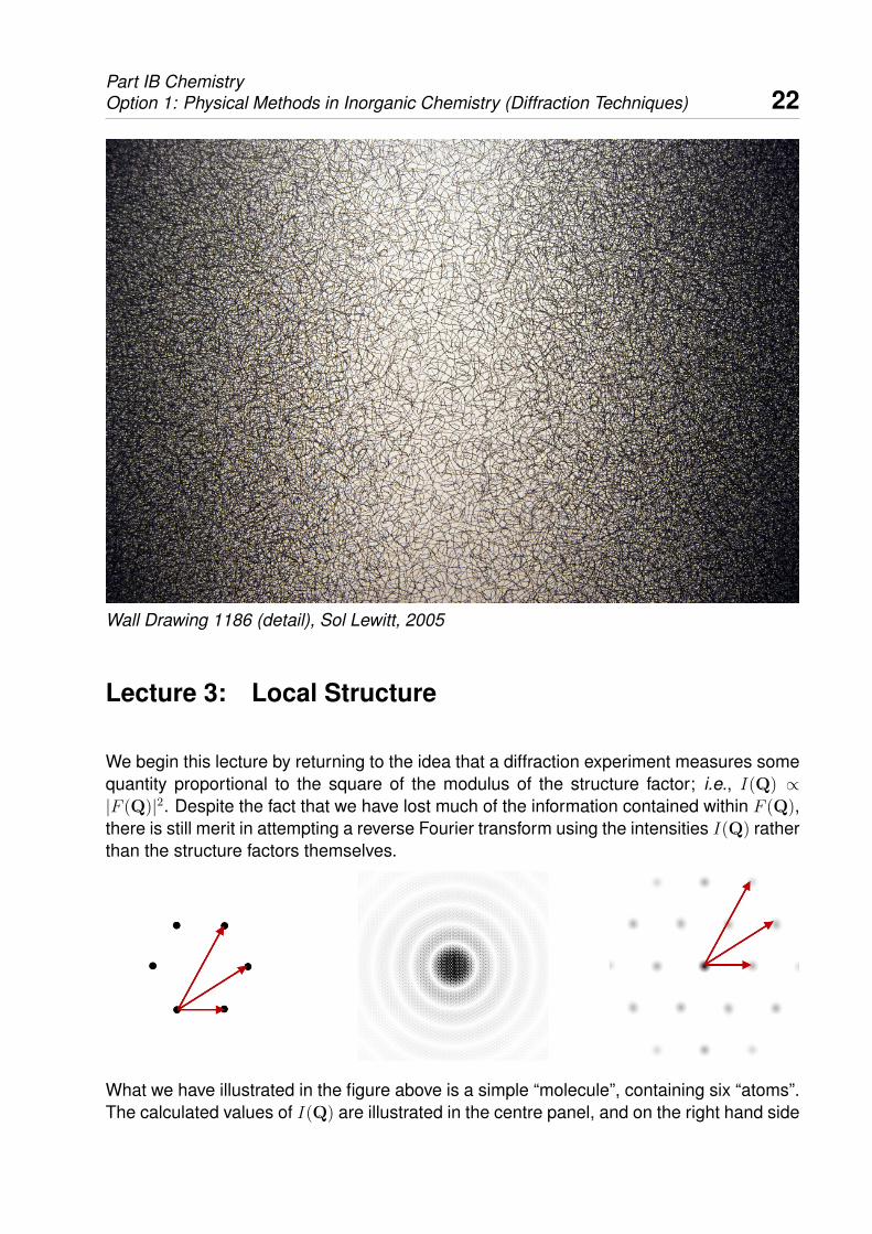
What we have illustrated in the figure above is a simple “molecule”, containing six “atoms”.The calculated values of I(Q) are illustrated in the centre panel, and on the right hand side


we see the reverse Fourier transform of this intensity information — a so-called “Pattersonmap”. A Patterson map will contain a peak for each interatomic vector in the originalstructure. So here we have many more peaks than there are atoms in the molecule, buteach peak can still be attributed to a pair of atoms in the molecule itself. We can see whythis works if we consider the mathematics involved (neglecting thermal motion or atomicscattering factors, for simplicity):

I(Q) ∝ |F (Q)|2 =

∣∣∣∣∫ ρ(r) exp(iQ · r) dr

∣∣∣∣2 (33)

=

∫ρ(r) exp(iQ · r) dr×

∫ρ(r) exp(−iQ · r) dr (34)

=

∫∫ρ(rj − ri) exp[iQ · (rj − ri)] dri drj. (35)

So the intensities reflect information about the separations of all pairs of particles, ratherthan their absolute positions. It is these separations that we recover in a Patterson map.Historically, such maps played an important role in the early methods of crystal structuresolution. Dorothy Hodgkin was one of the key pioneers, and it was her method of workingback from the Patterson map to the most likely positions of atoms that allowed her todetermine the structure of vitamin B12 — work for which she was awarded the Nobel prizein Chemistry in 1964.

A similar function, termed the pair distribution function (often abbreviated to PDF) can alsobe obtained from powder samples, except here the orientational information is lost. ThePDF is given the symbol g(r), and is defined such that the number of atoms with separationbetween r and r+dr is given as 4πr2ρ0g(r) dr. Here ρ0 is the number density of the sample;i.e. the number of atoms per unit volume. In the limit of large r, where the relative positionsof atoms are essentially independent, we have g(r) = 1 — the same value expected for astatistical (random) distribution of particles. At distances smaller than the sum of atomicradii, there can be no pairs of atoms, and we have g(r) = 0. There will be peaks in theg(r) function around the various distances that correspond to local separations, includingbond lengths and/or contact distances. The area under each peak will be related to thenumber of such contacts. For the nearest-neighbour interactions, this provides a handleon the coordination numbers:

coordination number =

∫ r,max

r,min

4πr2ρ0g(r) dr. (36)

Much as in Eq. (35) the powder-averaged scattering pattern S(Q) one would measure in adiffraction experiment is related to the PDF via:

S(Q) = 1 +4πρ0

Q

∫ ∞0

[g(r)− 1]r sin(Qr) dr. (37)

This relationship is invertible so that we can write g(r) in terms of S(Q):

g(r) = 1 +1

2π2ρ0r

∫ ∞0

Q[S(Q)− 1] sin(Qr) dQ. (38)


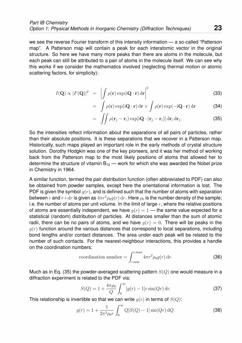
What this tells us that we can obtain a measure of g(r) directly from measurements ofS(Q). One application of these equations is to study bonding and local order even innon-crystalline materials such as silica glass (SiO2). In the figure above we show pair dis-tribution data for SiO2 (in the form of a frequently-used function T (r) = 4πrg(r)) extractedfrom S(Q) measurements. The first peak in T (r) is centred on 1.6 A, which is the size ofthe Si–O bond length in crystalline silicates. The integral of the first peak is consistent witheach silicon atom being bonded to four oxygen atoms. The peak at 3.0 A is the shortestSi–Si distance, and indicates that the Si–O–Si bond subtends an angle of ∼ 145◦.

For the same reasons discussed in Lecture 2, the PDF resolution in real-space is deter-mined by the value of Qmax for the diffraction experiment. Neutron diffractometers such asthe GEM instrument at ISIS are capable of measuring S(Q) to very large values of Q '40 A−1, and this has meant such instruments are ideal for PDF measurements. The inter-est in PDF arises mainly because it is one of the very few techniques available for studyingthe structure in materials with no long-range periodicity, or where the local structure issubstantially different from that deduced from “traditional” crystallographic approaches.

One other such technique is known as “extended x-ray absorption fine structure” (EXAFS),which is essentially a form of x-ray absorption spectroscopy. The basic principle is asfollows. A tuneable beam of x-rays is fired at a sample sample using x-ray energies thatare close to the K-edge absorption energy of a specific element in the sample. The K-edge energy is of course that required to dissociate a core 1s electron from the targetelement: it scales approximately as E0 ' Z2.16 so that speecific elements can easily betargeted individually. For x-ray energies slightly higher than E0, the photoejected electronwill end up with some remnant momentum such that its wavefunction is characterised by awave-vector with magnitude

k =

√2me(E − E0)

~2. (39)


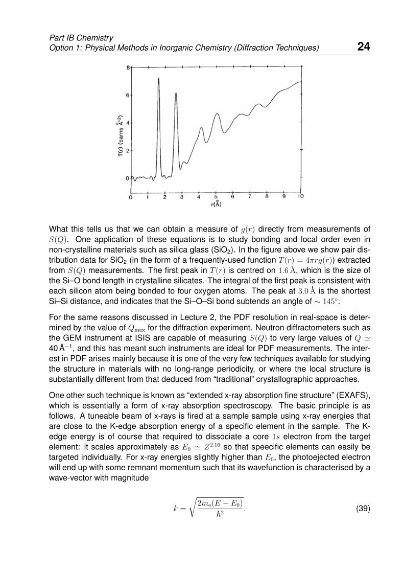
The wavefunction of this photoejected electron will interact with those of the neighbouringatoms, and the scattering processes involved can yield either constructive or destructiveinterference depending how well the periodicity given by k matches the arrangement ofthese neighbours. In turn this means that absorption is more likely at some energies thanat others, and one observes a modulation in the x-ray absorption spectrum at energiesgreater than E0.

We can analyse these “post-edge” oscillations by normalising the absorption function µ(E):

χ(E) =µ(E)− µ0

µ0

(40)

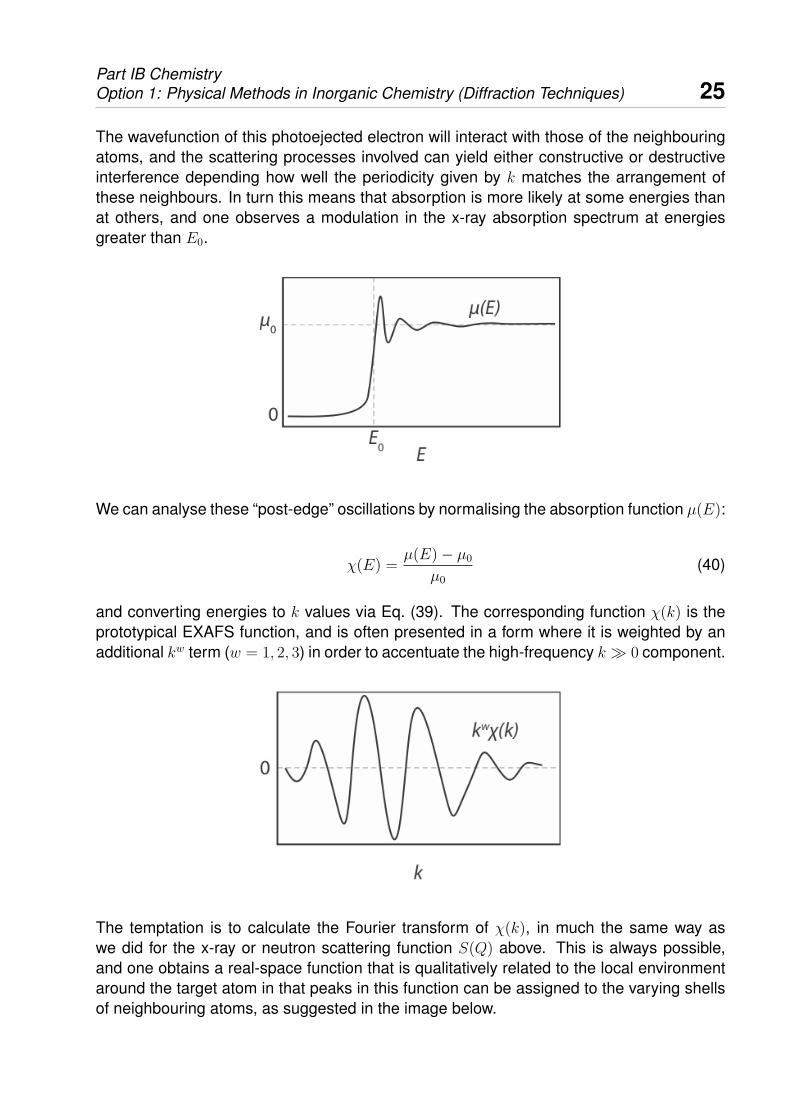
and converting energies to k values via Eq. (39). The corresponding function χ(k) is theprototypical EXAFS function, and is often presented in a form where it is weighted by anadditional kw term (w = 1, 2, 3) in order to accentuate the high-frequency k � 0 component.

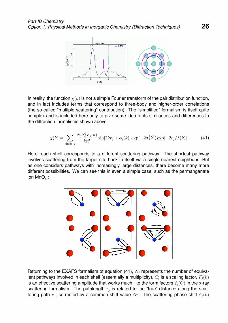
The temptation is to calculate the Fourier transform of χ(k), in much the same way aswe did for the x-ray or neutron scattering function S(Q) above. This is always possible,and one obtains a real-space function that is qualitatively related to the local environmentaround the target atom in that peaks in this function can be assigned to the varying shellsof neighbouring atoms, as suggested in the image below.


In reality, the function χ(k) is not a simple Fourier transform of the pair distribution function,and in fact includes terms that correspond to three-body and higher-order correlations(the so-called “multiple scattering” contribution). The “simplified” formalism is itself quitecomplex and is included here only to give some idea of its similarities and differences tothe diffraction formalisms shown above.

χ(k) =∑

shells j

NjS20Fj(k)

kr2j

sin[2krj + φj(k)] exp(−2σ2jk

2) exp[−2rj/λ(k)] (41)

Here, each shell corresponds to a different scattering pathway. The shortest pathwayinvolves scattering from the target site back to itself via a single nearest neighbour. Butas one considers pathways with increasingly large distances, there become many moredifferent possibilities. We can see this in even a simple case, such as the permanganateion MnO−4 :

Returning to the EXAFS formalism of equation (41), Nj represents the number of equiva-lent pathways involved in each shell (essentially a multiplicity), S2

0 is a scaling factor, Fj(k)

is an effective scattering amplitude that works much like the form factors fj(Q) in the x-rayscattering formalism. The pathlength rj is related to the “true” distance along the scat-tering path r0, corrected by a common shift value ∆r. The scattering phase shift φj(k)


can be calculated for each shell, as can the mean-free path λ(k). Finally, the values σjare measures of the mean-squared displacements of the atoms in each shell, and so theterm exp(−2σ2

jk2) works just like a Debye-Waller factor. Most of this is not critically impor-

tant here; what is important is that the formalism is almost a sine Fourier transform of thescattering density around the target centre, but unfortunately is not quite so simple.

In terms of the practical use of EXAFS as a probe of local structure, we note the following:

(i) EXAFS does not require long-range periodicity, so the technique is applicable toglasses or amorphous materials in exactly the same way as for crystalline materials.Likewise it can also be used with liquids or even gases.

(ii) Because it is element specific, it provides a way of targeting specific sites within astructure. This is especially useful in biological systems such as metalloprortiens,where the metal centre is usually critical for function.

(iii) Because tuneable x-ray energies are needed, EXAFS requires synchrotron radiation.It is not an in-house experimental technique.

(iv) Often multiple scattering effects end up dominating the EXAFS signal and this meansthat extraction of a unique structural model is usually impossible. The method is oftenmore definitively useful for invalidating than for validating models.

In class we will work through some examples of systems where EXAFS and pair distribu-tion function methods have provided insight into important scientific problems in a numberof different fields.


Color Equation, Pamela Nelson, 2007

Lecture 4: Worked Examples

In second year, you learned how to index cubic diffraction patterns: converting d-spacingsto 1/d2 values; renormalising so that the first reflection is given a value equal to 1; lookingfor a common factor needed to make all values integral; then using N = h2 + k2 + l2 toassign hkl indices to each reflection. Things are not so simple for non-cubic structures,and we begin this lecture by looking at how one might go about indexing the diffractionpatterns of tetragonal and hexagonal crystal systems. In general, it is worth remarkingthat indexing by hand — such as we will undertake here — is all but impossible for crystalsystems of lower symmetry. There are automated methods of indexing available for suchcases, but if the unit cell is quite large or the symmetry sufficiently low even these can runinto difficulties.

We are going to document here some of the formalisms involved, even though there is noexpectation at all that you learn these by heart. We begin by putting Q = ha∗ + kb∗ + c∗

and recalling that Q = 2π/d, such that


1

d2=

Q2

4π2=|ha∗ + kb∗ + lc∗|2

4π2(42)

This is a very general equation, and is true irrespective of the crystal symmetry: we havemade no assumptions here. The term on the numerator involves working out the modulusof a vector in reciprocal space, and the complications arise when the reciprocal lattice vec-tors a∗,b∗, c∗ are not mutually perpendicular. What we are going to do now is to evaluatethis expression for the tetragonal and hexagonal cases, working through from the deriva-tion of the reciprocal lattice vectors themselves. To do this we express the reciprocal latticevectors in terms of their components along the cartesian axes. Starting with the tetragonalcase, we have

a = ai

b = aj

c = ck (43)

Although we could leap ahead and exploit the fact that these three axes are orthogonal tosimplify Eq. (42), let us take our time so that things are more obvious when it comes to thehexagonal case. Recalling Eq. (6), we have:

a∗ =2π(b× c)

a · (b× c)

=

2π det

i j k

0 a 0

0 0 c

/ai · det

i j k

0 a 0

0 0 c

= {2πac i}

/{a2c}

=2π

ai (44)

(Note that I am taking it for granted here that all are happy with calculating vector crossproducts. The method I am using — namely taking the determinant of a suitable 3 × 3

matrix — is just my own preferred method, and if you have your own way of doing this,that is fine (so long as it works every time!) As an exercise, it might be worth checkingthat you also get the same results for the other two reciprocal lattice vectors: b∗ = 2π

aj and

c∗ = 2πck.)

Substituting these expressions into Eq. (42) we obtain

1

d2=

∣∣2πha

i + 2πka

j + 2πlc

k∣∣2

4π2

=h2 + k2

a2+l2

c2, (45)


which is the general expression we will use for tetragonal systems. Note that calculatingterm in the numerator is now straightforward because the unit vectors i, j,k are certainlymutually perpendicular.

For a hexagonal system, it is conventional to arrange the axes such that

a = ai

b = −a2i +

√3a

2j

c = ck (46)

Proceeding as before to evaluate the reciprocal lattice vectors, we obtain (taking a deepbreath here)

a∗ =2π(b× c)

a · (b× c)

=

2π det

i j k

−a2

√3a2

0

0 0 c

/ai · det

i j k

−a2

√3a2

0

0 0 c

=

{2π

(√3ac

2i +

ac

2j

)}/{√3

2a2c

}=

2π

ai +

2π√3a

j. (47)

We leave as an exercise the derivations b∗ = 4π√3a

j and c∗ = 2πck, and return to Eq. (42):

1

d2=

∣∣∣2πha i + 2π√3a

(h+ 2k)j + 2πlc

k∣∣∣2

4π2

=h2

a2+h2 + 4hk + 4k2

3a2+l2

c2

=4(h2 + hk + k2)

3a2+l2

c2, (48)

which is now the expression we will use for hexagonal systems (and indeed you will seequoted in past papers). It is not necessary that you know how to do these derivations forthe exam, but sometimes it is useful to see from where they come nonetheless.

Let us turn to some examples now, and consider first the tetragonal crystal TiO2 (rutile).Given the list of d-spacings below, our likely task is to try and assign hkl values to eachreflection, and to use this information to calculate the unit cell parameters. The first two


steps in our approach would be identical to the method we are used to using for cubic sys-tems: we convert d-spacings to 1/d2 values and then renormalise so that the first reflectionis given a value equal to 1. I call these renormalised values Σ, because in the cubic casethey should equal the sum h2 + k2 + l2; another common label is N , but you should feelfree to use whatever you like. There is no fixed convention.

d (A) 1/d2 (A−2) Σ Σ′ = 2Σ

3.2482 0.0948 1 22.4871 0.1617 1.7057 3.41142.2969 0.1896 2 42.1871 0.2091 2.2057 4.41142.0544 0.2369 2.5 51.6874 0.3512 3.7049 7.40981.6241 0.3791 4 81.4791 0.4571 4.8217 9.64341.4527 0.4739 5 101.4237 0.4934 5.2046 10.40921.3599 0.5408 5.7046 11.40921.3461 0.5519 5.8217 11.6434

The hope is that the first reflection will be either of the type (hk0) or (00l): this is often thecase since the highest d-spacing reflections tend to have the lowest hkl indices. By renor-malising against this reflection, we expect to see integral Σ values for any other reflectionsof the same type (hk0) or (00l), respectively: in the first instance Σ = h2 + k2 + (a

c)2l2; and

in the second Σ = l2 + ( ca)2(h2 + k2).

In this case we notice two things in the normalised values Σ. First, we end up with onereflection having Σ = 2.5. Second, there are two pairs of reflections for which the Σ valuesdiffer by 0.5: d = 2.4871, 2.1871 and d = 1.4237, 1.3599. What this is telling us is thatwe need to multiply our Σ values by 2 in order to make things integral. We now have fivereflections that are of the same type as the first reflection, with Σ′ = 2Σ values equal to2, 4, 5, 8 and 10. We have to decide whether we think we are dealing with (hk0) or (00l)

reflections here. In the former case, we would have Σ′ = h2 +k2, and it is possible to assignh, k values that satisfy all five reflections. In the latter case we have Σ′ = l2, and here weclearly run into problems. So we can say with some confidence that we are looking at (hk0)

reflections, and can assign all five: (110), (200), (210), (220), (310). We can also calculatea = 4.5937 A.

We have now assigned all the integral Σ′ reflections, and are left only with the tricky non-integral ones. We know that these are either of the form (00l) or (hkl). The first step isto identify which differ by integral values: these will be reflections with the same index l,but with different h and k values. Within the type of error we expect, we can say that thereare two groups: d = 2.4871, 2.1871, 1.6874, 1.4237, 1.3599 A all have Σ′ values endingin .4114 (or thereabouts); whereas d = 1.47911, 1.3461 A have Σ′ values ending in .6434.What we have to do now is to use these clues to work out what Σ′ value would correspond


to the basic reflection (001). Because the .4114 group occurs at larger d-spacings, the bestfirst guess is that l = 1 for all these reflections, while the .6434 reflections will correspondeither to l = 2 or even a higher index. If this guess is correct, we can say that Σ′(001) isa number of the form X.6434, with X = 3, 2, 1 or 0. Note that larger values of X are morelikely because we only see two orders of l 6= 0 reflections.

d (A) 1/d2 (A−2) Σ′ Σ′ − 3.4114 Σ′ − 2.4114

2.4871 0.1617 3.4114 0 12.1871 0.2091 4.4114 1 21.6874 0.3512 7.4098 4 51.4237 0.4934 10.4092 7 81.3599 0.5408 11.4092 8 9

The first temptation is to assign Σ′(001) = 3.4114. We subtract this value from the Σ′ valuesfor all the members of this group, and what we are checking to see now is if we can accountfor the remainder in terms of a suitable h2+k2 term. This is shown in the table above, wherewe see all is fine except for the fourth reflection in this group: there are no h and k valuessuch that h2 + k2 = 7. We can say now that the d = 2.4871 reflection is not (001).

The next possibility is that Σ′(001) = 2.4114, and again we subtract this value as above.We now find h2 + k2 terms for which we can account in all five cases: 1 = 1 + 0, 2 = 1 +1, 5 = 4 + 1, 8 = 4 + 4, 9 = 9 + 0. This seems to work well and we tentatively assign thereflections as (101), (111), (211), (221) and (301).

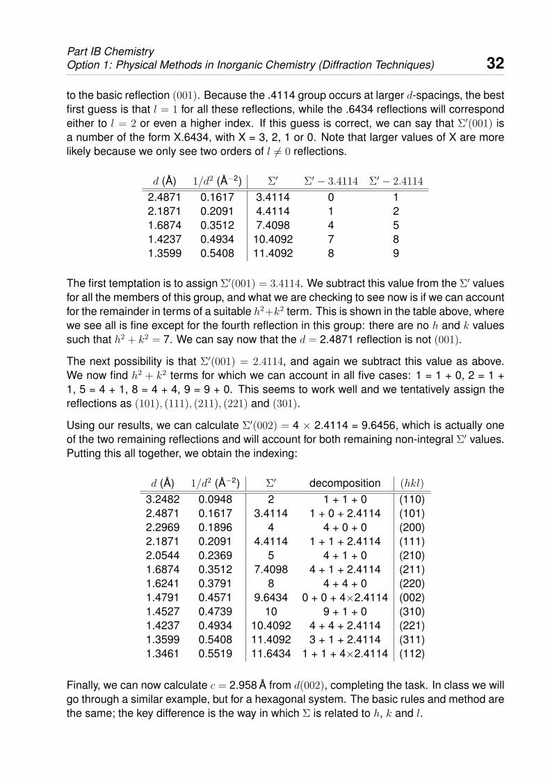
Using our results, we can calculate Σ′(002) = 4 × 2.4114 = 9.6456, which is actually oneof the two remaining reflections and will account for both remaining non-integral Σ′ values.Putting this all together, we obtain the indexing:

d (A) 1/d2 (A−2) Σ′ decomposition (hkl)

3.2482 0.0948 2 1 + 1 + 0 (110)2.4871 0.1617 3.4114 1 + 0 + 2.4114 (101)2.2969 0.1896 4 4 + 0 + 0 (200)2.1871 0.2091 4.4114 1 + 1 + 2.4114 (111)2.0544 0.2369 5 4 + 1 + 0 (210)1.6874 0.3512 7.4098 4 + 1 + 2.4114 (211)1.6241 0.3791 8 4 + 4 + 0 (220)1.4791 0.4571 9.6434 0 + 0 + 4×2.4114 (002)1.4527 0.4739 10 9 + 1 + 0 (310)1.4237 0.4934 10.4092 4 + 4 + 2.4114 (221)1.3599 0.5408 11.4092 3 + 1 + 2.4114 (311)1.3461 0.5519 11.6434 1 + 1 + 4×2.4114 (112)

Finally, we can now calculate c = 2.958 A from d(002), completing the task. In class we willgo through a similar example, but for a hexagonal system. The basic rules and method arethe same; the key difference is the way in which Σ is related to h, k and l.


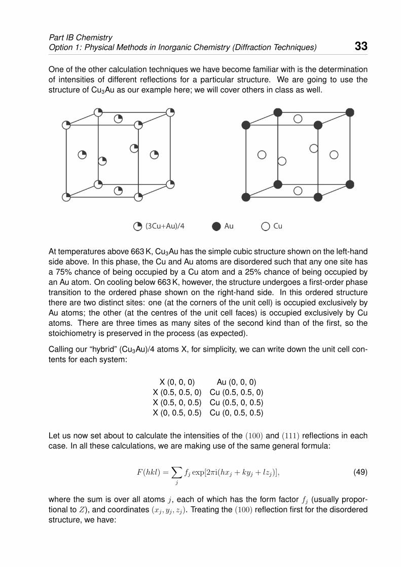
One of the other calculation techniques we have become familiar with is the determinationof intensities of different reflections for a particular structure. We are going to use thestructure of Cu3Au as our example here; we will cover others in class as well.

At temperatures above 663 K, Cu3Au has the simple cubic structure shown on the left-handside above. In this phase, the Cu and Au atoms are disordered such that any one site hasa 75% chance of being occupied by a Cu atom and a 25% chance of being occupied byan Au atom. On cooling below 663 K, however, the structure undergoes a first-order phasetransition to the ordered phase shown on the right-hand side. In this ordered structurethere are two distinct sites: one (at the corners of the unit cell) is occupied exclusively byAu atoms; the other (at the centres of the unit cell faces) is occupied exclusively by Cuatoms. There are three times as many sites of the second kind than of the first, so thestoichiometry is preserved in the process (as expected).

Calling our “hybrid” (Cu3Au)/4 atoms X, for simplicity, we can write down the unit cell con-tents for each system:

X (0, 0, 0) Au (0, 0, 0)X (0.5, 0.5, 0) Cu (0.5, 0.5, 0)X (0.5, 0, 0.5) Cu (0.5, 0, 0.5)X (0, 0.5, 0.5) Cu (0, 0.5, 0.5)

Let us now set about to calculate the intensities of the (100) and (111) reflections in eachcase. In all these calculations, we are making use of the same general formula:

F (hkl) =∑j

fj exp[2πi(hxj + kyj + lzj)], (49)

where the sum is over all atoms j, each of which has the form factor fj (usually propor-tional to Z), and coordinates (xj, yj, zj). Treating the (100) reflection first for the disorderedstructure, we have:


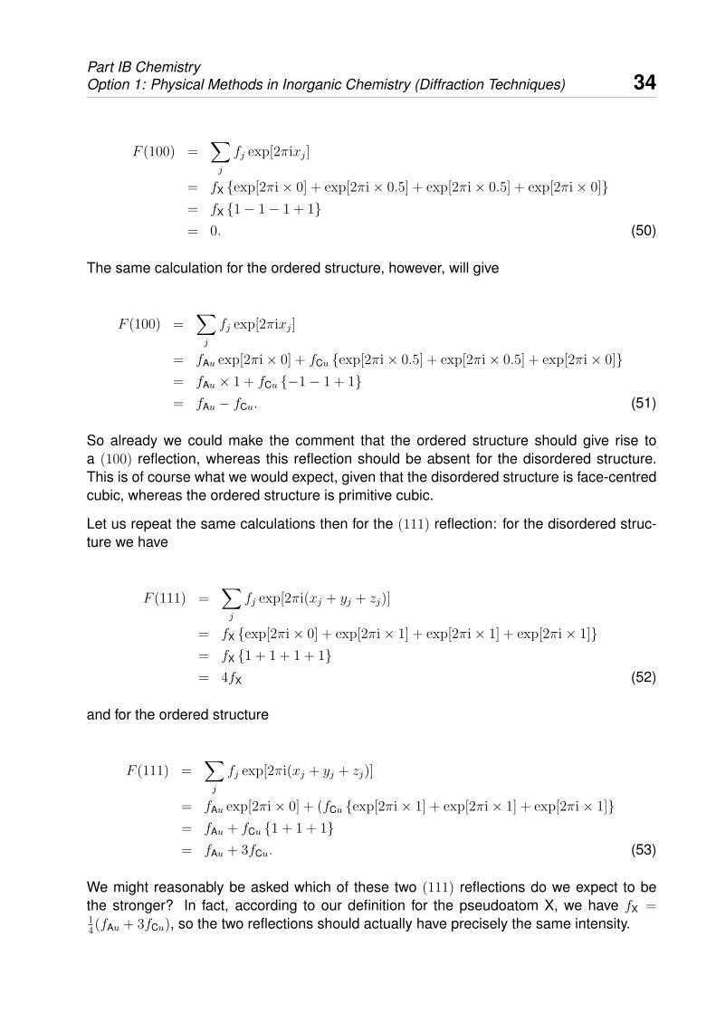
F (100) =∑j

fj exp[2πixj]

= fX {exp[2πi× 0] + exp[2πi× 0.5] + exp[2πi× 0.5] + exp[2πi× 0]}= fX {1− 1− 1 + 1}= 0. (50)

The same calculation for the ordered structure, however, will give

F (100) =∑j

fj exp[2πixj]

= fAu exp[2πi× 0] + fCu {exp[2πi× 0.5] + exp[2πi× 0.5] + exp[2πi× 0]}= fAu × 1 + fCu {−1− 1 + 1}= fAu − fCu. (51)

So already we could make the comment that the ordered structure should give rise toa (100) reflection, whereas this reflection should be absent for the disordered structure.This is of course what we would expect, given that the disordered structure is face-centredcubic, whereas the ordered structure is primitive cubic.

Let us repeat the same calculations then for the (111) reflection: for the disordered struc-ture we have

F (111) =∑j

fj exp[2πi(xj + yj + zj)]

= fX {exp[2πi× 0] + exp[2πi× 1] + exp[2πi× 1] + exp[2πi× 1]}= fX {1 + 1 + 1 + 1}= 4fX (52)

and for the ordered structure

F (111) =∑j

fj exp[2πi(xj + yj + zj)]

= fAu exp[2πi× 0] + (fCu {exp[2πi× 1] + exp[2πi× 1] + exp[2πi× 1]}= fAu + fCu {1 + 1 + 1}= fAu + 3fCu. (53)

We might reasonably be asked which of these two (111) reflections do we expect to bethe stronger? In fact, according to our definition for the pseudoatom X, we have fX =14(fAu + 3fCu), so the two reflections should actually have precisely the same intensity.


Exercises

(i) Consider a hexagonal lattice with unit cell vectors oriented relative to the cartesianunit vectors i, j, k as follows:

a = ai

b = −a2i +

√3a

2j

c = ck

Sketch the reciprocal lattice (assume c > a) and label the reciprocal lattice points.With reference to your sketch, explain why the d-spacings for the (100) and (110)

reflections would be identical.

(ii) Sketch the reciprocal lattice that corresponds to a face-centred cubic lattice in realspace. Label the reciprocal lattice points, remembering that the first reciprocal latticepoint along the a∗ direction may not be (100). How can you use your diagram tounderstand the systematic absences associated with F-centering?

(iii) KCl adopts the standard rocksalt structure, but contains the isoelectronic ions K+ andCl−. Sketch what you think the powder diffraction patterns might look like using (i)x-rays and (ii) neutrons, highlighting the most significant differences.

(iv) Centrosymmetric crystals are so-called because for each atom at a position (x, y, z)

there is an equivalent atom at (−x,−y,−z). Use this fact to show that all structurefactors F (hkl) for a centrosymmetric crystal are real-valued.

(v) Using appropriate sketches, indicate what you think the likely differences and similar-ities are amongst the pair distribution functions of crystalline, glassy and liquid formsof SiO2.

(vi) Find an example in the literature of where EXAFS and PDF methods have apparentlycontradicted one another. Comment on how this might occur, assuming the scientificintegrity of the researches concerned can be taken as read.

(vii) The d-spacings and intensities in the x-ray powder diffraction pattern of NaLiSO4 aregiven in the table below. Assign each reflection and give the Bravais lattice and unitcell parameters.

d (A) Intensity (arb.) d (A) Intensity (arb.)6.60518 2.6 3.01615 35.65.48728 2.8 2.94201 31.74.92895 0.5 2.74364 77.83.95031 60.2 2.49652 0.63.81350 100.0 2.46447 6.03.30259 3.2 2.42012 8.83.13152 2.1 2.32938 3.7


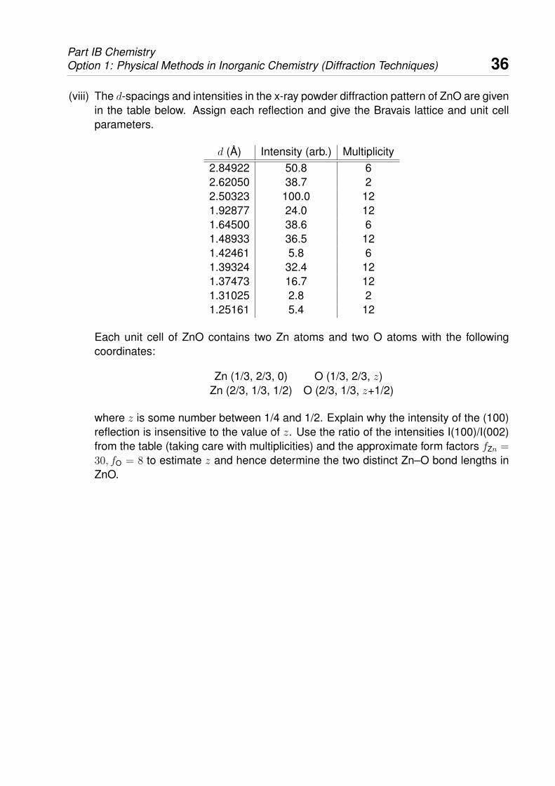
(viii) The d-spacings and intensities in the x-ray powder diffraction pattern of ZnO are givenin the table below. Assign each reflection and give the Bravais lattice and unit cellparameters.

d (A) Intensity (arb.) Multiplicity2.84922 50.8 62.62050 38.7 22.50323 100.0 121.92877 24.0 121.64500 38.6 61.48933 36.5 121.42461 5.8 61.39324 32.4 121.37473 16.7 121.31025 2.8 21.25161 5.4 12

Each unit cell of ZnO contains two Zn atoms and two O atoms with the followingcoordinates:

Zn (1/3, 2/3, 0) O (1/3, 2/3, z)Zn (2/3, 1/3, 1/2) O (2/3, 1/3, z+1/2)

where z is some number between 1/4 and 1/2. Explain why the intensity of the (100)reflection is insensitive to the value of z. Use the ratio of the intensities I(100)/I(002)from the table (taking care with multiplicities) and the approximate form factors fZn =

30, fO = 8 to estimate z and hence determine the two distinct Zn–O bond lengths inZnO.


Appendix: Convolution theorem

We say that the function f(x) is the convolution of two functions g(x) and h(x) if

f(x) =

∫g(x′)h(x− x′) dx′. (54)

We denote this relationship as f(x) = g(x)⊗h(x) (an alternative representation sometimesused is f = g ∗ h). The convolution is essentially an integral that expresses the amount ofoverlap of the function h(x) as it is shifted over the function g(x): it essentially “blends” onefunction with another.

The operation is commutative:

g(x)⊗ h(x) =

∫ ∞−∞

g(x′)h(x− x′) dx′

=

∫ −∞∞

g(x− x′′)h(x′′) · −dx′′ (x′′ = x− x′) (55)

=

∫ ∞−∞

h(x′′)g(x− x′′) dx′′ (56)

= h(x)⊗ g(x) (57)

Our key result actually concerns the Fourier transform of a convolution. Writing the trans-forms of our three functions f(x), g(x) and h(x) as F (k), G(k) and H(k), respectively, wehave:

F (k) =

∫f(x) exp(ikx)) dx (58)

=

∫g(x)⊗ h(x) exp(ikx) dx (59)

=

∫∫g(x′)h(x− x′) exp(ikx) dx′ dx (60)

=

∫∫g(x′)h(x− x′) exp[ik(x− x′)] exp(ikx′) dx′ dx (61)

=

∫g(x′) exp(ikx′) dx′ ×

∫h(x− x′) exp[ik(x− x′)] dx (62)

=

∫g(x′) exp(ikx′) dx′ ×

∫h(x′′) exp(ikx′′) dx′′ (x′′ = x− x′) (63)

= G(k)×H(k) (64)

Appendix: Reciprocal lattice derivation

Here we want to show that the Fourier transform of the one-dimensional lattice functionL(x) =

∑n δ(x − na) is given by the reciprocal lattice function R(Q) =

∑Q δ(Q − 2πh/a).

Let us define R(Q) as the Fourier transform of L(x). Then we have:


R(Q) =

∫L(x) exp(iQx) dx (65)

=

∫ ∑n

δ(x− na) exp(iQx) dx (66)

=∑n

∫δ(x− na) exp(iQx) dx (67)

Now, for each integral within the sum on the right-hand side of this equation we will partitionspace into two regions: that region such that x is less than a small distance ε from na, andall remaining values of x. That is,

R(Q) =∑n

[∫ ∞|x−na|=ε

δ(x− na) exp(iQx) dx

= +

∫ |x−na|=ε|x−na|=0

δ(x− na) exp(iQx) dx

](68)

=∑n

[0 + exp(iQna)] (69)

Now, for most Q, the summation on the right hand side will cancel over all values of n togive 0. The exception occurs whenever Q = 2πh/a (h an integer), in which case

R(Q) = R(h) =∑n

exp(2πinh)→∞ (70)

So R(Q) is a series of spikes located at Q = 2πh/a; that is

R(Q) =∑h

δ(Q− 2πh/a) (71)

as required.

Extending this to three dimensions we have L(r) =∑

UVW δ[r − (Ua + V b + Wc)]. ItsFourier transform is

R(Q) =

∫L(r) exp(iQ · r) dr (72)

=∑UVW

exp[iQ · (Ua + V b +Wc)] (73)

This function is now a three-dimensional set of δ-functions located at Q for which Q · (Ua+

b + c) is an integral multiple of 2π. Consider the vector


a∗ = 2πb× c

a · (b× c)(74)

Note that b× c is a vector perpendicular to both b and c so that a∗ · b = a∗ · c = 0 and

a∗ · a = 2πa · (b× c)

a · (b× c)= 2π (75)

So Q = ha∗ will satisfy the δ-function requirement for all integral h. Similarly, assigning

b∗ = 2πc× a

b · (c× a)(76)

and

c∗ = 2πa× b

c · (a× b)(77)

means that any integral combination Q = ha∗+kb∗+ lc∗ will also satisfy the requirements,giving

R(Q) =∑hkl

δ[Q− (ha∗ + kb∗ + lc∗)] (78)

as required.

Documents

Part IB Inorganic Chemistry Option 1: Physical Methods in ...goodwin.chem.ox.ac.uk/goodwin/TEACHING_files/alg_ib_diffraction.pdf · Part IB Chemistry Option 1: Physical Methods in