Embed Size (px)
Citation preview
Part IA — Probability
Based on lectures by R. WeberNotes taken by Dexter Chua
Lent 2015
These notes are not endorsed by the lecturers, and I have modified them (oftensignificantly) after lectures. They are nowhere near accurate representations of what
was actually lectured, and in particular, all errors are almost surely mine.
Basic conceptsClassical probability, equally likely outcomes. Combinatorial analysis, permutationsand combinations. Stirling’s formula (asymptotics for logn! proved). [3]
Axiomatic approachAxioms (countable case). Probability spaces. Inclusion-exclusion formula. Continuityand subadditivity of probability measures. Independence. Binomial, Poisson and geo-metric distributions. Relation between Poisson and binomial distributions. Conditionalprobability, Bayes’s formula. Examples, including Simpson’s paradox. [5]
Discrete random variablesExpectation. Functions of a random variable, indicator function, variance, standarddeviation. Covariance, independence of random variables. Generating functions: sumsof independent random variables, random sum formula, moments.
Conditional expectation. Random walks: gambler’s ruin, recurrence relations. Dif-ference equations and their solution. Mean time to absorption. Branching processes:generating functions and extinction probability. Combinatorial applications of generat-ing functions. [7]
Continuous random variablesDistributions and density functions. Expectations; expectation of a function of arandom variable. Uniform, normal and exponential random variables. Memorylessproperty of exponential distribution. Joint distributions: transformation of randomvariables (including Jacobians), examples. Simulation: generating continuous randomvariables, independent normal random variables. Geometrical probability: Bertrand’sparadox, Buffon’s needle. Correlation coefficient, bivariate normal random variables. [6]
Inequalities and limitsMarkov’s inequality, Chebyshev’s inequality. Weak law of large numbers. Convexity:Jensen’s inequality for general random variables, AM/GM inequality.
Moment generating functions and statement (no proof) of continuity theorem. State-
ment of central limit theorem and sketch of proof. Examples, including sampling. [3]
1
Contents IA Probability
Contents
0 Introduction 3
1 Classical probability 41.1 Classical probability . . . . . . . . . . . . . . . . . . . . . . . . . 41.2 Counting . . . . . . . . . . . . . . . . . . . . . . . . . . . . . . . 51.3 Stirling’s formula . . . . . . . . . . . . . . . . . . . . . . . . . . . 8
2 Axioms of probability 112.1 Axioms and definitions . . . . . . . . . . . . . . . . . . . . . . . . 112.2 Inequalities and formulae . . . . . . . . . . . . . . . . . . . . . . 132.3 Independence . . . . . . . . . . . . . . . . . . . . . . . . . . . . . 162.4 Important discrete distributions . . . . . . . . . . . . . . . . . . . 172.5 Conditional probability . . . . . . . . . . . . . . . . . . . . . . . 18
3 Discrete random variables 223.1 Discrete random variables . . . . . . . . . . . . . . . . . . . . . . 223.2 Inequalities . . . . . . . . . . . . . . . . . . . . . . . . . . . . . . 313.3 Weak law of large numbers . . . . . . . . . . . . . . . . . . . . . 333.4 Multiple random variables . . . . . . . . . . . . . . . . . . . . . . 343.5 Probability generating functions . . . . . . . . . . . . . . . . . . 37
4 Interesting problems 434.1 Branching processes . . . . . . . . . . . . . . . . . . . . . . . . . 434.2 Random walk and gambler’s ruin . . . . . . . . . . . . . . . . . . 46
5 Continuous random variables 505.1 Continuous random variables . . . . . . . . . . . . . . . . . . . . 505.2 Stochastic ordering and inspection paradox . . . . . . . . . . . . 545.3 Jointly distributed random variables . . . . . . . . . . . . . . . . 555.4 Geometric probability . . . . . . . . . . . . . . . . . . . . . . . . 575.5 The normal distribution . . . . . . . . . . . . . . . . . . . . . . . 595.6 Transformation of random variables . . . . . . . . . . . . . . . . 615.7 Moment generating functions . . . . . . . . . . . . . . . . . . . . 66
6 More distributions 686.1 Cauchy distribution . . . . . . . . . . . . . . . . . . . . . . . . . 686.2 Gamma distribution . . . . . . . . . . . . . . . . . . . . . . . . . 696.3 Beta distribution* . . . . . . . . . . . . . . . . . . . . . . . . . . 696.4 More on the normal distribution . . . . . . . . . . . . . . . . . . 706.5 Multivariate normal . . . . . . . . . . . . . . . . . . . . . . . . . 71
7 Central limit theorem 74
8 Summary of distributions 788.1 Discrete distributions . . . . . . . . . . . . . . . . . . . . . . . . . 788.2 Continuous distributions . . . . . . . . . . . . . . . . . . . . . . . 78
2
0 Introduction IA Probability
0 Introduction
In every day life, we often encounter the use of the term probability, and theyare used in many different ways. For example, we can hear people say:
(i) The probability that a fair coin will land heads is 1/2.
(ii) The probability that a selection of 6 members wins the National LotteryLotto jackpot is 1 in
(196
)= 13983816 or 7.15112× 10⁻⁸.
(iii) The probability that a drawing pin will land ’point up’ is 0.62.
(iv) The probability that a large earthquake will occur on the San AndreasFault in the next 30 years is about 21%
(v) The probability that humanity will be extinct by 2100 is about 50%
The first two cases are things derived from logic. For example, we know thatthe coin either lands heads or tails. By definition, a fair coin is equally likely toland heads or tail. So the probability of either must be 1/2.
The third is something probably derived from experiments. Perhaps we did1000 experiments and 620 of the pins point up. The fourth and fifth examplesbelong to yet another category that talks about are beliefs and predictions.
We call the first kind “classical probability”, the second kind “frequentistprobability” and the last “subjective probability”. In this course, we onlyconsider classical probability.
3
1 Classical probability IA Probability
1 Classical probability
We start with a rather informal introduction to probability. Afterwards, inChapter 2, we will have a formal axiomatic definition of probability and formallystudy their properties.
1.1 Classical probability
Definition (Classical probability). Classical probability applies in a situationwhen there are a finite number of equally likely outcome.
A classical example is the problem of points.
Example. A and B play a game in which they keep throwing coins. If a headlands, then A gets a point. Otherwise, B gets a point. The first person to get10 points wins a prize.
Now suppose A has got 8 points and B has got 7, but the game has to endbecause an earthquake struck. How should they divide the prize? We answerthis by finding the probability of A winning. Someone must have won by theend of 19 rounds, i.e. after 4 more rounds. If A wins at least 2 of them, then Awins. Otherwise, B wins.
The number of ways this can happen is(
42
)+(
43
)+(
44
)= 11, while there are
16 possible outcomes in total. So A should get 11/16 of the prize.
In general, consider an experiment that has a random outcome.
Definition (Sample space). The set of all possible outcomes is the sample space,Ω. We can lists the outcomes as ω1, ω2, · · · ∈ Ω. Each ω ∈ Ω is an outcome.
Definition (Event). A subset of Ω is called an event.
Example. When rolling a dice, the sample space is 1, 2, 3, 4, 5, 6, and eachitem is an outcome. “Getting an odd number” and “getting 3” are two possibleevents.
In probability, we will be dealing with sets a lot, so it would be helpful tocome up with some notation.
Definition (Set notations). Given any two events A,B ⊆ Ω,
– The complement of A is AC = A′ = A = Ω \A.
– “A or B” is the set A ∪B.
– “A and B” is the set A ∩B.
– A and B are mutually exclusive or disjoint if A ∩B = ∅.
– If A ⊆ B, then A occurring implies B occurring.
Definition (Probability). Suppose Ω = ω1, ω2, · · · , ωN. Let A ⊆ Ω be anevent. Then the probability of A is
P(A) =Number of outcomes in A
Number of outcomes in Ω=|A|N.
4
1 Classical probability IA Probability
Here we are assuming that each outcome is equally likely to happen, whichis the case in (fair) dice rolls and coin flips.
Example. Suppose r digits are drawn at random from a table of random digitsfrom 0 to 9. What is the probability that
(i) No digit exceeds k;
(ii) The largest digit drawn is k?
The sample space is Ω = (a1, a2, · · · , ar) : 0 ≤ ai ≤ 9. Then |Ω| = 10r.Let Ak = [no digit exceeds k] = (a1, · · · , ar) : 0 ≤ ai ≤ k. Then |Ak| =
(k + 1)r. So
P (Ak) =(k + 1)r
10r.
Now let Bk = [largest digit drawn is k]. We can find this by finding all outcomesin which no digits exceed k, and subtract it by the number of outcomes in whichno digit exceeds k − 1. So |Bk| = |Ak| − |Ak−1| and
P (Bk) =(k + 1)r − kr
10r.
1.2 Counting
To find probabilities, we often need to count things. For example, in our exampleabove, we had to count the number of elements in Bk.
Example. A menu has 6 starters, 7 mains and 6 desserts. How many possiblemeals combinations are there? Clearly 6× 7× 6 = 252.
Here we are using the fundamental rule of counting:
Theorem (Fundamental rule of counting). Suppose we have to make r multiplechoices in sequence. There are m1 possibilities for the first choice, m2 possibilitiesfor the second etc. Then the total number of choices is m1 ×m2 × · · ·mr.
Example. How many ways can 1, 2, · · · , n be ordered? The first choice has npossibilities, the second has n−1 possibilities etc. So there are n×(n−1)×· · ·×1 =n!.
Sampling with or without replacement
Suppose we have to pick n items from a total of x items. We can model this asfollows: Let N = 1, 2, · · · , n be the list. Let X = 1, 2, · · · , x be the items.Then each way of picking the items is a function f : N → X with f(i) = item atthe ith position.
Definition (Sampling with replacement). When we sample with replacement,after choosing at item, it is put back and can be chosen again. Then any samplingfunction f satisfies sampling with replacement.
Definition (Sampling without replacement). When we sample without replace-ment, after choosing an item, we kill it with fire and cannot choose it again.Then f must be an injective function, and clearly we must have x ≥ n.
5
1 Classical probability IA Probability
We can also have sampling with replacement, but we require each item to bechosen at least once. In this case, f must be surjective.
Example. Suppose N = a, b, c and X = p, q, r, s. How many injectivefunctions are there N → X?
When we choose f(a), we have 4 options. When we choose f(b), we have3 left. When we choose f(c), we have 2 choices left. So there are 24 possiblechoices.
Example. I have n keys in my pocket. We select one at random once and tryto unlock. What is the possibility that I succeed at the rth trial?
Suppose we do it with replacement. We have to fail the first r − 1 trials andsucceed in the rth. So the probability is
(n− 1)(n− 1) · · · (n− 1)(1)
nr=
(n− 1)r−1
nr.
Now suppose we are smarter and try without replacement. Then the probabilityis
(n− 1)(n− 2) · · · (n− r + 1)(1)
n(n− 1) · · · (n− r + 1)=
1
n.
Example (Birthday problem). How many people are needed in a room for thereto be a probability that two people have the same birthday to be at least a half?
Suppose f(r) is the probability that, in a room of r people, there is a birthdaymatch.
We solve this by finding the probability of no match, 1 − f(r). The totalnumber of possibilities of birthday combinations is 365r. For nobody to havethe same birthday, the first person can have any birthday. The second has 364else to choose, etc. So
P(no match) =365 · 364 · 363 · · · (366− r)
365 · 365 · 365 · · · 365.
If we calculate this with a computer, we find that f(22) = 0.475695 and f(23) =0.507297.
While this might sound odd since 23 is small, this is because we are thinkingabout the wrong thing. The probability of match is related more to the number ofpairs of people, not the number of people. With 23 people, we have 23× 22/2 =253 pairs, which is quite large compared to 365.
Sampling with or without regard to ordering
There are cases where we don’t care about, say list positions. For example, if wepick two representatives from a class, the order of picking them doesn’t matter.
In terms of the function f : N → X, after mapping to f(1), f(2), · · · , f(n),we can
– Leave the list alone
– Sort the list ascending. i.e. we might get (2, 5, 4) and (4, 2, 5). If we don’tcare about list positions, these are just equivalent to (2, 4, 5).
6
1 Classical probability IA Probability
– Re-number each item by the number of the draw on which it was first seen.For example, we can rename (2, 5, 2) and (5, 4, 5) both as (1, 2, 1). Thishappens if the labelling of items doesn’t matter.
– Both of above. So we can rename (2, 5, 2) and (8, 5, 5) both as (1, 1, 2).
Total number of cases
Combining these four possibilities with whether we have replacement, no replace-ment, or “everything has to be chosen at least once”, we have 12 possible casesof counting. The most important ones are:
– Replacement + with ordering: the number of ways is xn.
– Without replacement + with ordering: the number of ways is x(n) = xn =x(x− 1) · · · (x− n+ 1).
– Without replacement + without order: we only care which items getselected. The number of ways is
(xn
)= Cxn = x(n)/n!.
– Replacement + without ordering: we only care how many times the itemgot chosen. This is equivalent to partitioning n into n1 + n2 + · · · + nk.Say n = 6 and k = 3. We can write a particular partition as
∗∗ | ∗ | ∗ ∗ ∗
So we have n+ k − 1 symbols and k − 1 of them are bars. So the numberof ways is
(n+k−1k−1
).
Multinomial coefficient
Suppose that we have to pick n items, and each item can either be an apple oran orange. The number of ways of picking such that k apples are chosen is, bydefinition,
(nk
).
In general, suppose we have to fill successive positions in a list of lengthn, with replacement, from a set of k items. The number of ways of doing sosuch that item i is picked ni times is defined to be the multinomial coefficient(
nn1,n2,··· ,nk
).
Definition (Multinomial coefficient). A multinomial coefficient is(n
n1, n2, · · · , nk
)=
(n
n1
)(n− n1
n2
)· · ·(n− n1 · · · − nk−1
nk
)=
n!
n1!n2! · · ·nk!.
It is the number of ways to distribute n items into k positions, in which the ithposition has ni items.
Example. We know that
(x+ y)n = xn +
(n
1
)xn−1y + · · ·+ yn.
If we have a trinomial, then
(x+ y + z)n =∑
n1,n2,n3
(n
n1, n2, n3
)xn1yn2zn3 .
7
1 Classical probability IA Probability
Example. How many ways can we deal 52 cards to 4 player, each with a handof 13? The total number of ways is(
52
13, 13, 13, 13
)=
52!
(13!)4= 53644737765488792839237440000 = 5.36× 1028.
While computers are still capable of calculating that, what if we tried morepower cards? Suppose each person has n cards. Then the number of ways is
(4n)!
(n!)4,
which is huge. We can use Stirling’s Formula to approximate it:
1.3 Stirling’s formula
Before we state and prove Stirling’s formula, we prove a weaker (but examinable)version:
Proposition. log n! ∼ n log n
Proof. Note that
log n! =
n∑k=1
log k.
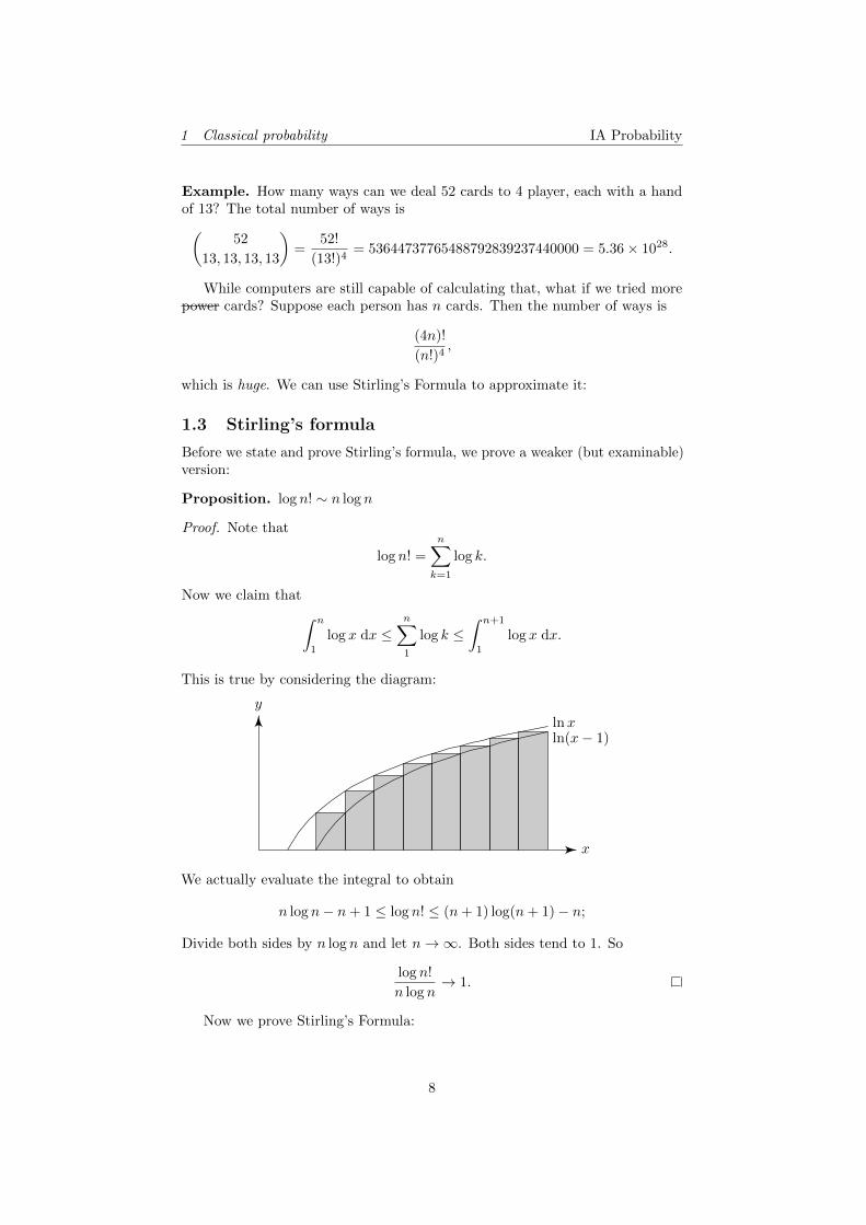
Now we claim that∫ n
1
log x dx ≤n∑1
log k ≤∫ n+1
1
log x dx.
This is true by considering the diagram:
x
y
lnxln(x− 1)
We actually evaluate the integral to obtain
n log n− n+ 1 ≤ log n! ≤ (n+ 1) log(n+ 1)− n;
Divide both sides by n log n and let n→∞. Both sides tend to 1. So
log n!
n log n→ 1.
Now we prove Stirling’s Formula:
8
1 Classical probability IA Probability
Theorem (Stirling’s formula). As n→∞,
log
(n!en
nn+ 12
)= log
√2π +O
(1
n
)Corollary.
n! ∼√
2πnn+ 12 e−n
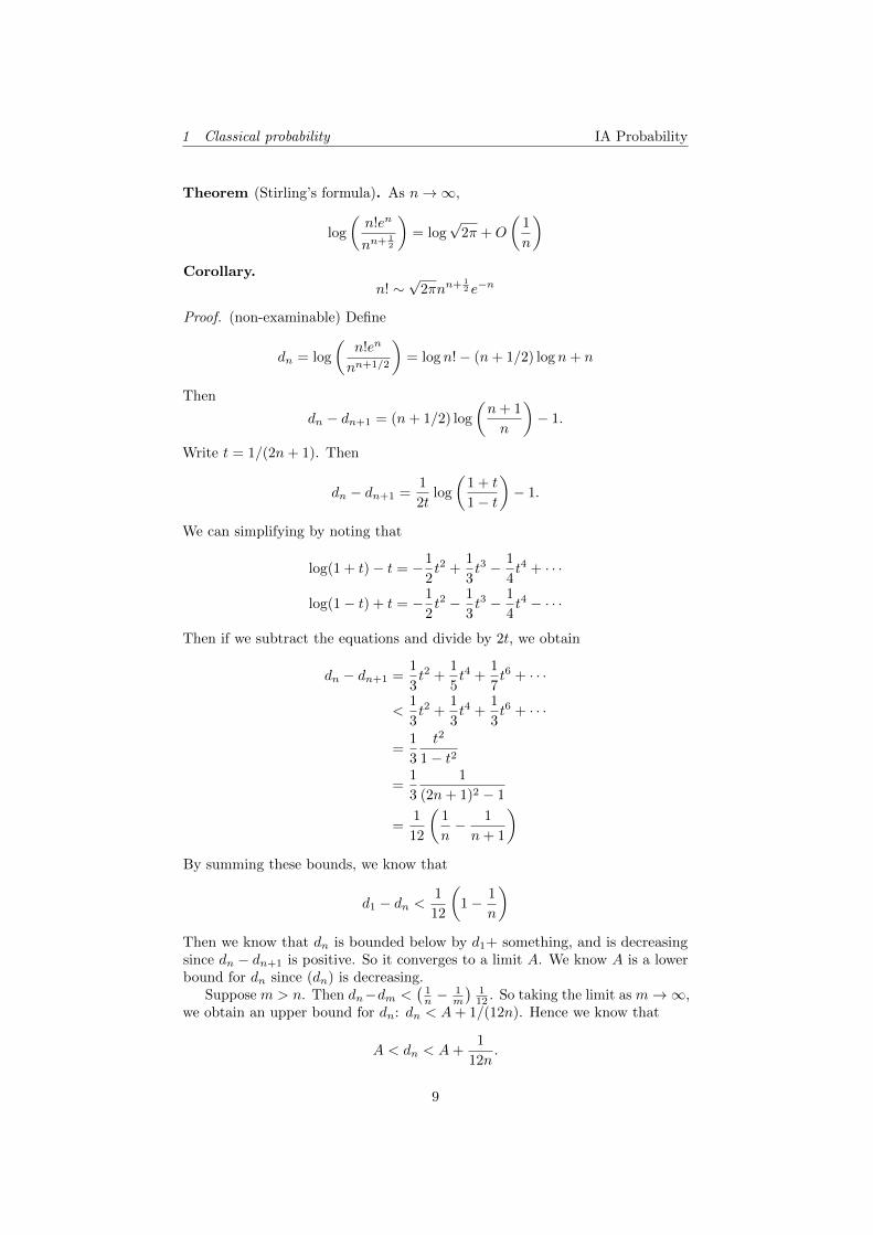
Proof. (non-examinable) Define
dn = log
(n!en
nn+1/2
)= log n!− (n+ 1/2) log n+ n
Then
dn − dn+1 = (n+ 1/2) log
(n+ 1
n
)− 1.
Write t = 1/(2n+ 1). Then
dn − dn+1 =1
2tlog
(1 + t
1− t
)− 1.
We can simplifying by noting that
log(1 + t)− t = −1
2t2 +
1
3t3 − 1
4t4 + · · ·
log(1− t) + t = −1
2t2 − 1
3t3 − 1
4t4 − · · ·
Then if we subtract the equations and divide by 2t, we obtain
dn − dn+1 =1
3t2 +
1
5t4 +
1
7t6 + · · ·
<1
3t2 +
1
3t4 +
1
3t6 + · · ·
=1
3
t2
1− t2
=1
3
1
(2n+ 1)2 − 1
=1
12
(1
n− 1
n+ 1
)By summing these bounds, we know that
d1 − dn <1
12
(1− 1
n
)Then we know that dn is bounded below by d1+ something, and is decreasingsince dn − dn+1 is positive. So it converges to a limit A. We know A is a lowerbound for dn since (dn) is decreasing.
Suppose m > n. Then dn−dm <(
1n −
1m
)112 . So taking the limit as m→∞,
we obtain an upper bound for dn: dn < A+ 1/(12n). Hence we know that
A < dn < A+1
12n.
9
1 Classical probability IA Probability
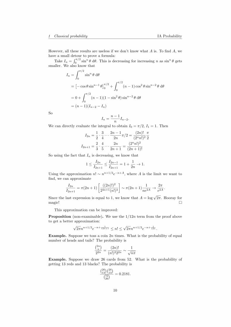
However, all these results are useless if we don’t know what A is. To find A, wehave a small detour to prove a formula:
Take In =∫ π/2
0sinn θ dθ. This is decreasing for increasing n as sinn θ gets
smaller. We also know that
In =
∫ π/2
0
sinn θ dθ
=[− cos θ sinn−1 θ
]π/20
+
∫ π/2
0
(n− 1) cos2 θ sinn−2 θ dθ
= 0 +
∫ π/2
0
(n− 1)(1− sin2 θ) sinn−2 θ dθ
= (n− 1)(In−2 − In)
So
In =n− 1
nIn−2.
We can directly evaluate the integral to obtain I0 = π/2, I1 = 1. Then
I2n =1
2· 3
4· · · 2n− 1
2nπ/2 =
(2n)!
(2nn!)2
π
2
I2n+1 =2
3· 4
5· · · 2n
2n+ 1=
(2nn!)2
(2n+ 1)!
So using the fact that In is decreasing, we know that
1 ≤ I2nI2n+1
≤ I2n−1
I2n+1= 1 +
1
2n→ 1.
Using the approximation n! ∼ nn+1/2e−n+A, where A is the limit we want tofind, we can approximate
I2nI2n+1
= π(2n+ 1)
[((2n)!)2
24n+1(n!)4
]∼ π(2n+ 1)
1
ne2A→ 2π
e2A.
Since the last expression is equal to 1, we know that A = log√
2π. Hooray formagic!
This approximation can be improved:
Proposition (non-examinable). We use the 1/12n term from the proof aboveto get a better approximation:
√2πnn+1/2e−n+ 1
12n+1 ≤ n! ≤√
2πnn+1/2e−n+ 112n .
Example. Suppose we toss a coin 2n times. What is the probability of equalnumber of heads and tails? The probability is(
2nn
)22n
=(2n)!
(n!)222n∼ 1√
nπ
Example. Suppose we draw 26 cards from 52. What is the probability ofgetting 13 reds and 13 blacks? The probability is(
2613
)(2613
)(5226
) = 0.2181.
10
2 Axioms of probability IA Probability
2 Axioms of probability
2.1 Axioms and definitions
So far, we have semi-formally defined some probabilistic notions. However, whatwe had above was rather restrictive. We were only allowed to have a finitenumber of possible outcomes, and all outcomes occur with the same probability.However, most things in the real world do not fit these descriptions. For example,we cannot use this to model a coin that gives heads with probability π−1.
In general, “probability” can be defined as follows:
Definition (Probability space). A probability space is a triple (Ω,F ,P). Ω is aset called the sample space, F is a collection of subsets of Ω, and P : F → [0, 1]is the probability measure.F has to satisfy the following axioms:
(i) ∅,Ω ∈ F .
(ii) A ∈ F ⇒ AC ∈ F .
(iii) A1, A2, · · · ∈ F ⇒⋃∞i=1Ai ∈ F .
And P has to satisfy the following Kolmogorov axioms:
(i) 0 ≤ P(A) ≤ 1 for all A ∈ F
(ii) P(Ω) = 1
(iii) For any countable collection of events A1, A2, · · · which are disjoint, i.e.Ai ∩Aj = ∅ for all i, j, we have
P
(⋃i
Ai
)=∑i
P(Ai).
Items in Ω are known as the outcomes, items in F are known as the events, andP(A) is the probability of the event A.
If Ω is finite (or countable), we usually take F to be all the subsets of Ω, i.e.the power set of Ω. However, if Ω is, say, R, we have to be a bit more carefuland only include nice subsets, or else we cannot have a well-defined P.
Often it is not helpful to specify the full function P. Instead, in discrete cases,we just specify the probabilities of each outcome, and use the third axiom toobtain the full P.
Definition (Probability distribution). Let Ω = ω1, ω2, · · · . Choose numbersp1, p2, · · · such that
∑∞i=1 pi = 1. Let p(ωi) = pi. Then define
P(A) =∑ωi∈A
p(ωi).
This P(A) satisfies the above axioms, and p1, p2, · · · is the probability distribution
Using the axioms, we can quickly prove a few rather obvious results.
Theorem.
11
2 Axioms of probability IA Probability
(i) P(∅) = 0
(ii) P(AC) = 1− P(A)
(iii) A ⊆ B ⇒ P(A) ≤ P(B)
(iv) P(A ∪B) = P(A) + P(B)− P(A ∩B).
Proof.
(i) Ω and ∅ are disjoint. So P(Ω) + P(∅) = P(Ω ∪ ∅) = P(Ω). So P(∅) = 0.
(ii) P(A) + P(AC) = P(Ω) = 1 since A and AC are disjoint.
(iii) Write B = A ∪ (B ∩AC). ThenP (B) = P(A) + P(B ∩AC) ≥ P(A).
(iv) P(A ∪ B) = P(A) + P(B ∩ AC). We also know that P(B) = P(A ∩ B) +P(B ∩AC). Then the result follows.
From above, we know that P(A ∪B) ≤ P(A) + P(B). So we say that P is asubadditive function. Also, P(A ∩B) + P(A ∪B) ≤ P(A) + P(B) (in fact bothsides are equal!). We say P is submodular.
The next theorem is better expressed in terms of limits.
Definition (Limit of events). A sequence of events A1, A2, · · · is increasing ifA1 ⊆ A2 · · · . Then we define the limit as
limn→∞
An =
∞⋃1
An.
Similarly, if they are decreasing, i.e. A1 ⊇ A2 · · · , then
limn→∞
An =
∞⋂1
An.
Theorem. If A1, A2, · · · is increasing or decreasing, then
limn→∞
P(An) = P(
limn→∞
An
).
Proof. Take B1 = A1, B2 = A2 \A1. In general,
Bn = An \n−1⋃
1
Ai.
Thenn⋃1
Bi =
n⋃1
Ai,
∞⋃1
Bi =
∞⋃1
Ai.
12
2 Axioms of probability IA Probability
Then
P(limAn) = P
(∞⋃1
Ai
)
= P
(∞⋃1
Bi
)
=
∞∑1
P(Bi) (Axiom III)
= limn→∞
n∑i=1
P(Bi)
= limn→∞
P
(n⋃1
Ai
)= limn→∞
P(An).
and the decreasing case is proven similarly (or we can simply apply the above toACi ).
2.2 Inequalities and formulae
Theorem (Boole’s inequality). For any A1, A2, · · · ,
P
( ∞⋃i=1
Ai
)≤∞∑i=1
P(Ai).
This is also known as the “union bound”.
Proof. Our third axiom states a similar formula that only holds for disjoint sets.So we need a (not so) clever trick to make them disjoint. We define
B1 = A1
B2 = A2 \A1
Bi = Ai \i−1⋃k=1
Ak.
So we know that ⋃Bi =
⋃Ai.
But the Bi are disjoint. So our Axiom (iii) gives
P
(⋃i
Ai
)= P
(⋃i
Bi
)=∑i
P (Bi) ≤∑i
P (Ai) .
Where the last inequality follows from (iii) of the theorem above.
Example. Suppose we have countably infinite number of biased coins. LetAk = [kth toss head] and P(Ak) = pk. Suppose
∑∞1 pk < ∞. What is the
probability that there are infinitely many heads?
13
2 Axioms of probability IA Probability
The event “there is at least one more head after the ith coin toss” is⋃∞k=iAk.
There are infinitely many heads if and only if there are unboundedly many cointosses, i.e. no matter how high i is, there is still at least more more head afterthe ith toss.
So the probability required is
P
( ∞⋂i=1
∞⋃k=i
Ak
)= limi→∞
P
( ∞⋃k=i
Ak
)≤ limi→∞
∞∑k=i
pk = 0
Therefore P(infinite number of heads) = 0.
Example (Erdos 1947). Is it possible to colour a complete n-graph (i.e. a graphof n vertices with edges between every pair of vertices) red and black such thatthere is no k-vertex complete subgraph with monochrome edges?
Erdos said this is possible if(n
k
)21−(k2) < 1.
We colour edges randomly, and let Ai = [ith subgraph has monochrome edges].Then the probability that at least one subgraph has monochrome edges is
P(⋃
Ai
)≤∑
P(Ai) =
(n
k
)2 · 2−(k2).
The last expression is obtained since there are(nk
)ways to choose a subgraph; a
monochrome subgraph can be either red or black, thus the multiple of 2; and
the probability of getting all red (or black) is 2−(k2).If this probability is less than 1, then there must be a way to colour them in
which it is impossible to find a monochrome subgraph, or else the probability is
1. So if(nk
)21−(k2) < 1, the colouring is possible.
Theorem (Inclusion-exclusion formula).
P
(n⋃i
Ai
)=
n∑1
P(Ai)−∑i1<i2
P(Ai1 ∩Aj2) +∑
i1<i2<i3
P(Ai1 ∩Ai2 ∩Ai3)− · · ·
+ (−1)n−1P(A1 ∩ · · · ∩An).
Proof. Perform induction on n. n = 2 is proven above.Then
P(A1 ∪A2 ∪ · · ·An) = P(A1) + P(A2 ∪ · · · ∪An)− P
(n⋃i=2
(A1 ∩Ai)
).
Then we can apply the induction hypothesis for n − 1, and expand the mess.The details are very similar to that in IA Numbers and Sets.
Example. Let 1, 2, · · · , n be randomly permuted to π(1), π(2), · · · , π(n). Ifi 6= π(i) for all i, we say we have a derangement.
Let Ai = [i 6= π(i)].
14
2 Axioms of probability IA Probability
Then
P
(n⋃i=1
Ai
)=∑k
P(Ak)−∑k1<k2
P(Ak1 ∩Ak2) + · · ·
= n · 1
n−(n
2
)1
n
1
n− 1+
(n
3
)1
n
1
n− 1
1
n− 2+ · · ·
= 1− 1
2!+
1
3!− · · ·+ (−1)n−1 1
n!
→ e−1
So the probability of derangement is 1− P(⋃Ak) ≈ 1− e−1 ≈ 0.632.
Recall that, from inclusion exclusion,
P(A ∪B ∪ C) = P(A) + P(B) + P(C)− P(AB)− P(BC)− P(AC) + P(ABC),
where P(AB) is a shorthand for P(A ∩B). If we only take the first three terms,then we get Boole’s inequality
P(A ∪B ∪ C) ≤ P(A) + P(B) + P(C).
In general
Theorem (Bonferroni’s inequalities). For any events A1, A2, · · · , An and 1 ≤r ≤ n, if r is odd, then
P
(n⋃1
Ai
)≤∑i1
P(Ai1)−∑i1<i2
P(Ai1Ai2) +∑
i1<i2<i3
P(Ai1Ai2Ai3) + · · ·
+∑
i1<i2<···<ir
P(Ai1Ai2Ai3 · · ·Air ).
If r is even, then
P
(n⋃1
Ai
)≥∑i1
P(Ai1)−∑i1<i2
P(Ai1Ai2) +∑
i1<i2<i3
P(Ai1Ai2Ai3) + · · ·
−∑
i1<i2<···<ir
P(Ai1Ai2Ai3 · · ·Air ).
Proof. Easy induction on n.
Example. Let Ω = 1, 2, · · · ,m and 1 ≤ j, k ≤ m. Write Ak = 1, 2, · · · , k.Then
Ak ∩Aj = 1, 2, · · · ,min(j, k) = Amin(j,k)
andAk ∪Aj = 1, 2, · · · ,max(j, k) = Amax(j,k).
We also have P(Ak) = k/m.Now let 1 ≤ x1, · · · , xn ≤ m be some numbers. Then Bonferroni’s inequality
says
P(⋃
Axi
)≥∑
P(Axi)−∑i<j
P(Axi ∩Axj ).
Somaxx1, x2, · · · , xn ≥
∑xi −
∑i1<i2
minx1, x2.
15
2 Axioms of probability IA Probability
2.3 Independence
Definition (Independent events). Two events A and B are independent if
P(A ∩B) = P(A)P(B).
Otherwise, they are said to be dependent.
Two events are independent if they are not related to each other. For example,if you roll two dice separately, the outcomes will be independent.
Proposition. If A and B are independent, then A and BC are independent.
Proof.
P(A ∩BC) = P(A)− P(A ∩B)
= P(A)− P(A)P(B)
= P(A)(1− P(B))
= P(A)P(BC)
This definition applies to two events. What does it mean to say that threeor more events are independent?
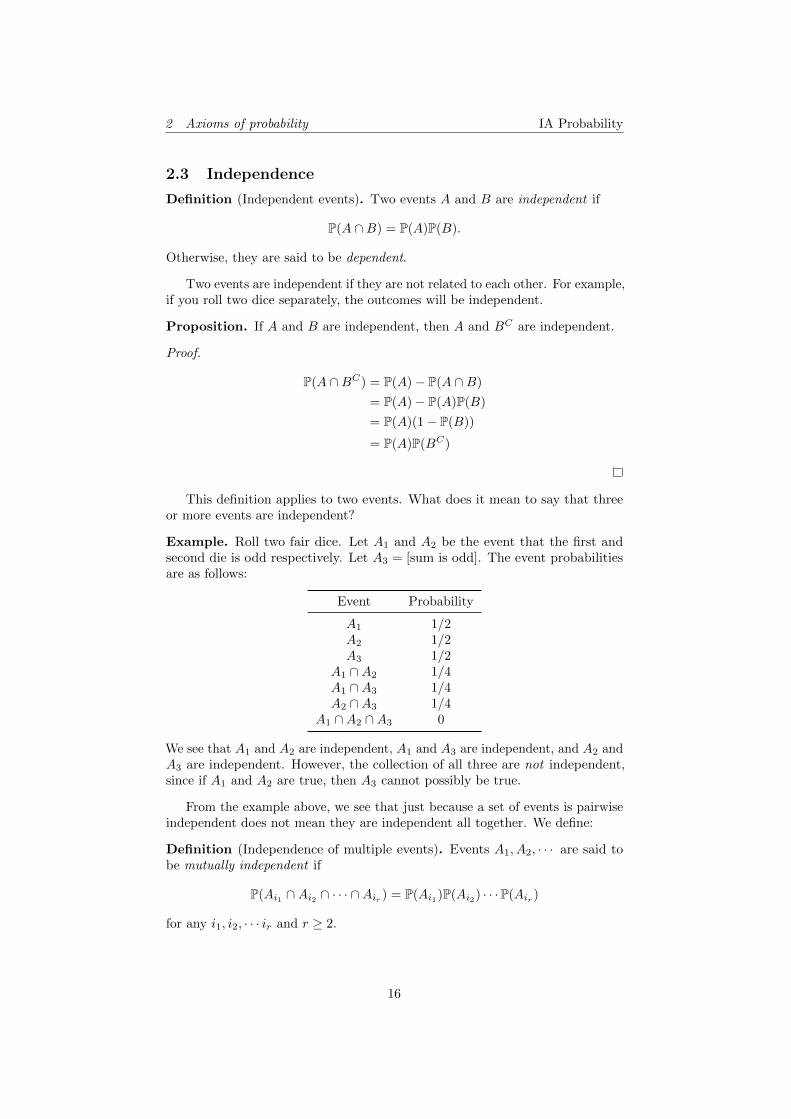
Example. Roll two fair dice. Let A1 and A2 be the event that the first andsecond die is odd respectively. Let A3 = [sum is odd]. The event probabilitiesare as follows:
Event Probability
A1 1/2A2 1/2A3 1/2
A1 ∩A2 1/4A1 ∩A3 1/4A2 ∩A3 1/4
A1 ∩A2 ∩A3 0
We see that A1 and A2 are independent, A1 and A3 are independent, and A2 andA3 are independent. However, the collection of all three are not independent,since if A1 and A2 are true, then A3 cannot possibly be true.
From the example above, we see that just because a set of events is pairwiseindependent does not mean they are independent all together. We define:
Definition (Independence of multiple events). Events A1, A2, · · · are said tobe mutually independent if
P(Ai1 ∩Ai2 ∩ · · · ∩Air ) = P(Ai1)P(Ai2) · · ·P(Air )
for any i1, i2, · · · ir and r ≥ 2.
16
2 Axioms of probability IA Probability
Example. Let Aij be the event that i and j roll the same. We roll 4 dice. Then
P(A12 ∩A13) =1
6· 1
6=
1
36= P(A12)P(A13).
But
P(A12 ∩A13 ∩A23) =1
366= P(A12)P(A13)P(A23).
So they are not mutually independent.
We can also apply this concept to experiments. Suppose we model twoindependent experiments with Ω1 = α1, α2, · · · and Ω2 = β1, β2, · · · withprobabilities P(αi) = pi and P(βi) = qi. Further suppose that these twoexperiments are independent, i.e.
P((αi, βj)) = piqj
for all i, j. Then we can have a new sample space Ω = Ω1 × Ω2.Now suppose A ⊆ Ω1 and B ⊆ Ω2 are results (i.e. events) of the two
experiments. We can view them as subspaces of Ω by rewriting them as A× Ω2
and Ω1 ×B. Then the probability
P(A ∩B) =∑
αi∈A,βi∈B
piqi =∑αi∈A
pi∑βi∈B
qi = P(A)P(B).
So we say the two experiments are “independent” even though the term usuallyrefers to different events in the same experiment. We can generalize this to nindependent experiments, or even countably many infinite experiments.
2.4 Important discrete distributions
We’re now going to quickly go through a few important discrete probabilitydistributions. By discrete we mean the sample space is countable. The samplespace is Ω = ω1, ω2, · · · and pi = P(ωi).
Definition (Bernoulli distribution). Suppose we toss a coin. Ω = H,T andp ∈ [0, 1]. The Bernoulli distribution, denoted B(1, p) has
P(H) = p; P(T ) = 1− p.
Definition (Binomial distribution). Suppose we toss a coin n times, each withprobability p of getting heads. Then
P(HHTT · · ·T ) = pp(1− p) · · · (1− p).
So
P(two heads) =
(n
2
)p2(1− p)n−2.
In general,
P(k heads) =
(n
k
)pk(1− p)n−k.
We call this the binomial distribution and write it as B(n, p).
17
2 Axioms of probability IA Probability
Definition (Geometric distribution). Suppose we toss a coin with probability pof getting heads. The probability of having a head after k consecutive tails is
pk = (1− p)kp
This is geometric distribution. We say it is memoryless because how many tailswe’ve got in the past does not give us any information to how long I’ll have towait until I get a head.
Definition (Hypergeometric distribution). Suppose we have an urn with n1 redballs and n2 black balls. We choose n balls. The probability that there are kred balls is
P(k red) =
(n1
k
)(n2
n−k)(
n1+n2
n
) .
Definition (Poisson distribution). The Poisson distribution denoted P (λ) is
pk =λk
k!e−λ
for k ∈ N.
What is this weird distribution? It is a distribution used to model rare events.Suppose that an event happens at a rate of λ. We can think of this as therebeing a lot of trials, say n of them, and each has a probability λ/n of succeeding.As we take the limit n→∞, we obtain the Poisson distribution.
Theorem (Poisson approximation to binomial). Suppose n → ∞ and p → 0such that np = λ. Then
qk =
(n
k
)pk(1− p)n−k → λk
k!e−λ.
Proof.
qk =
(n
k
)pk(1− p)n−k
=1
k!
n(n− 1) · · · (n− k + 1)
nk(np)k
(1− np
n
)n−k→ 1
k!λke−λ
since (1− a/n)n → e−a.
2.5 Conditional probability
Definition (Conditional probability). Suppose B is an event with P(B) > 0.For any event A ⊆ Ω, the conditional probability of A given B is
P(A | B) =P(A ∩B)
P(B).
We interpret as the probability of A happening given that B has happened.
18
2 Axioms of probability IA Probability
Note that if A and B are independent, then
P(A | B) =P(A ∩B)
P(B)=
P(A)P(B)
P(B)= P(A).
Example. In a game of poker, let Ai = [player i gets royal flush]. Then
P(A1) = 1.539× 10⁻⁶.
andP(A2 | A1) = 1.969× 10⁻⁶.
It is significantly bigger, albeit still incredibly tiny. So we say “good handsattract”.
If P(A | B) > P(A), then we say that B attracts A. Since
P(A ∩B)
P(B)> P(A)⇔ P(A ∩B)
P(A)> P(B),
A attracts B if and only if B attracts A. We can also say A repels B if A attractsBC .
Theorem.
(i) P(A ∩B) = P(A | B)P(B).
(ii) P(A ∩B ∩ C) = P(A | B ∩ C)P(B | C)P(C).
(iii) P(A | B ∩ C) = P(A∩B|C)P(B|C) .
(iv) The function P( · | B) restricted to subsets of B is a probability function(or measure).
Proof. Proofs of (i), (ii) and (iii) are trivial. So we only prove (iv). To provethis, we have to check the axioms.
(i) Let A ⊆ B. Then P(A | B) = P(A∩B)P(B) ≤ 1.
(ii) P(B | B) = P(B)P(B) = 1.
(iii) Let Ai be disjoint events that are subsets of B. Then
P
(⋃i
Ai
∣∣∣∣∣B)
=P(⋃iAi ∩B)
P(B)
=P (⋃iAi)
P(B)
=∑ P(Ai)
P(B)
=∑ P(Ai ∩B)
P(B)
=∑
P(Ai | B).
19
2 Axioms of probability IA Probability
Definition (Partition). A partition of the sample space is a collection of disjointevents Bi∞i=0 such that
⋃iBi = Ω.
For example, “odd” and “even” partition the sample space into two events.The following result should be clear:
Proposition. If Bi is a partition of the sample space, and A is any event, then
P(A) =
∞∑i=1
P(A ∩Bi) =
∞∑i=1
P(A | Bi)P(Bi).
Example. A fair coin is tossed repeatedly. The gambler gets +1 for head, and−1 for tail. Continue until he is broke or achieves $a. Let
px = P(goes broke | starts with $x),
and B1 be the event that he gets head on the first toss. Then
px = P(B1)px+1 + P(BC1 )px−1
px =1
2px+1 +
1
2px−1
We have two boundary conditions p0 = 1, pa = 0. Then solving the recurrencerelation, we have
px = 1− x
a.
Theorem (Bayes’ formula). Suppose Bi is a partition of the sample space, andA and Bi all have non-zero probability. Then for any Bi,
P(Bi | A) =P(A | Bi)P(Bi)∑j P(A | Bj)P(Bj)
.
Note that the denominator is simply P(A) written in a fancy way.
Example (Screen test). Suppose we have a screening test that tests whether apatient has a particular disease. We denote positive and negative results as +and − respectively, and D denotes the person having disease. Suppose that thetest is not absolutely accurate, and
P(+ | D) = 0.98
P(+ | DC) = 0.01
P(D) = 0.001.
So what is the probability that a person has the disease given that he received apositive result?
P(D | +) =P(+ | D)P(D)
P(+ | D)P(D) + P(+ | DC)P(DC)
=0.98 · 0.001
0.98 · 0.001 + 0.01 · 0.999
= 0.09
So this test is pretty useless. Even if you get a positive result, since the disease isso rare, it is more likely that you don’t have the disease and get a false positive.
20
2 Axioms of probability IA Probability
Example. Consider the two following cases:
(i) I have 2 children, one of whom is a boy.
(ii) I have two children, one of whom is a son born on a Tuesday.
What is the probability that both of them are boys?
(i) P(BB | BB ∪BG) = 1/41/4+2/4 = 1
3 .
(ii) Let B∗ denote a boy born on a Tuesday, and B a boy not born on aTuesday. Then
P(B∗B∗ ∪B∗B | BB∗ ∪B∗B∗ ∪B∗G) =114 ·
114 + 2 · 1
14 ·614
114 ·
114 + 2 · 1
14 ·614 + 2 · 1
14 ·12
=13
27.
How can we understand this? It is much easier to have a boy born on a Tuesdayif you have two boys than one boy. So if we have the information that a boyis born on a Tuesday, it is now less likely that there is just one boy. In otherwords, it is more likely that there are two boys.
21
3 Discrete random variables IA Probability
3 Discrete random variables
With what we’ve got so far, we are able to answer questions like “what is theprobability of getting a heads?” or “what is the probability of getting 10 headsin a row?”. However, we cannot answer questions like “what do we expect toget on average?”. What does it even mean to take the average of a “heads” anda “tail”?
To make some sense of this notion, we have to assign, to each outcome, anumber. For example, if let “heads” correspond to 1 and “tails” correspond to 0.Then on average, we can expect to get 0.5. This is the idea of a random variable.
3.1 Discrete random variables
Definition (Random variable). A random variable X taking values in a set ΩXis a function X : Ω→ ΩX . ΩX is usually a set of numbers, e.g. R or N.
Intuitively, a random variable assigns a “number” (or a thing in ΩX) to eachevent (e.g. assign 6 to the event “dice roll gives 6”).
Definition (Discrete random variables). A random variable is discrete if ΩX isfinite or countably infinite.
Notation. Let T ⊆ ΩX , define
P(X ∈ T ) = P(ω ∈ Ω : X(ω) ∈ T).
i.e. the probability that the outcome is in T .
Here, instead of talking about the probability of getting a particular outcomeor event, we are concerned with the probability of a random variable taking aparticular value. If Ω is itself countable, then we can write this as
P(X ∈ T ) =∑
ω∈Ω:X(ω)∈T
pω.
Example. Let X be the value shown by rolling a fair die. Then ΩX =1, 2, 3, 4, 5, 6. We know that
P(X = i) =1
6.
We call this the discrete uniform distribution.
Definition (Discrete uniform distribution). A discrete uniform distributionis a discrete distribution with finitely many possible outcomes, in which eachoutcome is equally likely.
Example. Suppose we roll two dice, and let the values obtained by X and Y .Then the sum can be represented by X + Y , with
ΩX+Y = 2, 3, · · · , 12.
This shows that we can add random variables to get a new random variable.
22
3 Discrete random variables IA Probability
Notation. We writePX(x) = P(X = x).
We can also write X ∼ B(n, p) to mean
P(X = r) =
(n
r
)pr(1− p)n−r,
and similarly for the other distributions we have come up with before.
Definition (Expectation). The expectation (or mean) of a real-valued X isequal to
E[X] =∑ω∈Ω
pωX(ω).
provided this is absolutely convergent. Otherwise, we say the expectation doesn’texist. Alternatively,
E[X] =∑x∈ΩX
∑ω:X(ω)=x
pωX(ω)
=∑x∈ΩX
x∑
ω:X(ω)=x
pω
=∑x∈ΩX
xP (X = x).
We are sometimes lazy and just write EX.
This is the “average” value of X we expect to get. Note that this definitiononly holds in the case where the sample space Ω is countable. If Ω is continuous(e.g. the whole of R), then we have to define the expectation as an integral.
Example. Let X be the sum of the outcomes of two dice. Then
E[X] = 2 · 1
36+ 3 · 2
36+ · · ·+ 12 · 1
36= 7.
Note that E[X] can be non-existent if the sum is not absolutely convergent.However, it is possible for the expected value to be infinite:
Example (St. Petersburg paradox). Suppose we play a game in which we keeptossing a coin until you get a tail. If you get a tail on the ith round, then I payyou $2i. The expected value is
E[X] =1
2· 2 +
1
4· 4 +
1
8· 8 + · · · =∞.
This means that on average, you can expect to get an infinite amount of money!In real life, though, people would hardly be willing to pay $20 to play this game.There are many ways to resolve this paradox, such as taking into account thefact that the host of the game has only finitely many money and thus your realexpected gain is much smaller.
Example. We calculate the expected values of different distributions:
23
3 Discrete random variables IA Probability
(i) Poisson P (λ). Let X ∼ P (λ). Then
PX(r) =λre−λ
r!.
So
E[X] =
∞∑r=0
rP (X = r)
=
∞∑r=0
rλre−λ
r!
=
∞∑r=1
λλr−1e−λ
(r − 1)!
= λ
∞∑r=0
λre−λ
r!
= λ.
(ii) Let X ∼ B(n, p). Then
E[X] =
n∑0
rP (x = r)
=
n∑0
r
(n
r
)pr(1− p)n−r
=
n∑0
rn!
r!(n− r)!pr(1− p)n−r
= np
n∑r=1
(n− 1)!
(r − 1)![(n− 1)− (r − 1)]!pr−1(1− p)(n−1)−(r−1)
= np
n−1∑0
(n− 1
r
)pr(1− p)n−1−r
= np.
Given a random variable X, we can create new random variables such asX + 3 or X2. Formally, let f : R→ R and X be a real-valued random variable.Then f(X) is a new random variable that maps ω 7→ f(X(ω)).
Example. if a, b, c are constants, then a+bX and (X−c)2 are random variables,defined as
(a+ bX)(ω) = a+ bX(ω)
(X − c)2(ω) = (X(ω)− c)2.
Theorem.
(i) If X ≥ 0, then E[X] ≥ 0.
24
3 Discrete random variables IA Probability
(ii) If X ≥ 0 and E[X] = 0, then P(X = 0) = 1.
(iii) If a and b are constants, then E[a+ bX] = a+ bE[X].
(iv) If X and Y are random variables, then E[X + Y ] = E[X] + E[Y ]. This istrue even if X and Y are not independent.
(v) E[X] is a constant that minimizes E[(X − c)2] over c.
Proof.
(i) X ≥ 0 means that X(ω) ≥ 0 for all ω. Then
E[X] =∑ω
pωX(ω) ≥ 0.
(ii) If there exists ω such that X(ω) > 0 and pω > 0, then E[X] > 0. SoX(ω) = 0 for all ω.
(iii)
E[a+ bX] =∑ω
(a+ bX(ω))pω = a+ b∑ω
pω = a+ b E[X].
(iv)
E[X+Y ] =∑ω
pω[X(ω)+Y (ω)] =∑ω
pωX(ω)+∑ω
pωY (ω) = E[X]+E[Y ].
(v)
E[(X − c)2] = E[(X − E[X] + E[X]− c)2]
= E[(X − E[X])2 + 2(E[X]− c)(X − E[X]) + (E[X]− c)2]
= E(X − E[X])2 + 0 + (E[X]− c)2.
This is clearly minimized when c = E[X]. Note that we obtained the zeroin the middle because E[X − E[X]] = E[X]− E[X] = 0.
An easy generalization of (iv) above is
Theorem. For any random variables X1, X2, · · ·Xn, for which the followingexpectations exist,
E
[n∑i=1
Xi
]=
n∑i=1
E[Xi].
Proof.∑ω
p(ω)[X1(ω) + · · ·+Xn(ω)] =∑ω
p(ω)X1(ω) + · · ·+∑ω
p(ω)Xn(ω).
Definition (Variance and standard deviation). The variance of a randomvariable X is defined as
var(X) = E[(X − E[X])2].
The standard deviation is the square root of the variance,√
var(X).
25
3 Discrete random variables IA Probability
This is a measure of how “dispersed” the random variable X is. If we have alow variance, then the value of X is very likely to be close to E[X].
Theorem.
(i) varX ≥ 0. If varX = 0, then P(X = E[X]) = 1.
(ii) var(a+ bX) = b2 var(X). This can be proved by expanding the definitionand using the linearity of the expected value.
(iii) var(X) = E[X2]− E[X]2, also proven by expanding the definition.
Example (Binomial distribution). Let X ∼ B(n, p) be a binomial distribution.Then E[X] = np. We also have
E[X(X − 1)] =
n∑r=0
r(r − 1)n!
r!(n− r)!pr(1− p)n−r
= n(n− 1)p2n∑r=2
(n− 2
r − 2
)pr−2(1− p)(n−2)−(r−2)
= n(n− 1)p2.
The sum goes to 1 since it is the sum of all probabilities of a binomial N(n−2, p)So E[X2] = n(n− 1)p2 + E[X] = n(n− 1)p2 + np. So
var(X) = E[X2]− (E[X])2 = np(1− p) = npq.
Example (Poisson distribution). If X ∼ P (λ), then E[X] = λ, and var(X) = λ,since P (λ) is B(n, p) with n→∞, p→ 0, np→ λ.
Example (Geometric distribution). Suppose P(X = r) = qrp for r = 0, 1, 2, · · · .Then
E[X] =
∞∑0
rpqr
= pq
∞∑0
rqr−1
= pq
∞∑0
d
dqqr
= pqd
dq
∞∑0
qr
= pqd
dq
1
1− q=
pq
(1− q)2
=q
p.
26
3 Discrete random variables IA Probability
Then
E[X(X − 1)] =
∞∑0
r(r − 1)pqr
= pq2∞∑0
r(r − 1)qr−2
= pq2 d2
dq2
1
1− q
=2pq2
(1− q)3
So the variance is
var(X) =2pq2
(1− q)3+q
p− q2
p2=
q
p2.
Definition (Indicator function). The indicator function or indicator variableI[A] (or IA) of an event A ⊆ Ω is
I[A](ω) =
1 ω ∈ A0 ω 6∈ A
This indicator random variable is not interesting by itself. However, it is arather useful tool to prove results.
It has the following properties:
Proposition.
– E[I[A]] =∑ω p(ω)I[A](ω) = P(A).
– I[AC ] = 1− I[A].
– I[A ∩B] = I[A]I[B].
– I[A ∪B] = I[A] + I[B]− I[A]I[B].
– I[A]2 = I[A].
These are easy to prove from definition. In particular, the last propertycomes from the fact that I[A] is either 0 and 1, and 02 = 0, 12 = 1.
Example. Let 2n people (n husbands and n wives, with n > 2) sit alternateman-woman around the table randomly. Let N be the number of couples sittingnext to each other.
Let Ai = [ith couple sits together]. Then
N =
n∑i=1
I[Ai].
Then
E[N ] = E[∑
I[Ai]]
=
n∑1
E[I[Ai]
]= nE
[I[A1]
]= nP(Ai) = n · 2
n= 2.
27
3 Discrete random variables IA Probability
We also have
E[N2] = E[(∑
I[Ai])2]
= E
∑i
I[Ai]2 + 2
∑i<j
I[Ai]I[Aj ]
= nE
[I[Ai]
]+ n(n− 1)E
[I[A1]I[A2]
]We have E[I[A1]I[A2]] = P(A1 ∩ A2) = 2
n
(1
n−11
n−1 + n−2n−1
2n−1
). Plugging in,
we ultimately obtain var(N) = 2(n−2)n−1 .
In fact, as n→∞, N ∼ P (2).
We can use these to prove the inclusion-exclusion formula:
Theorem (Inclusion-exclusion formula).
P
(n⋃i
Ai
)=
n∑1
P(Ai)−∑i1<i2
P(Ai1 ∩Aj2) +∑
i1<i2<i3
P(Ai1 ∩Ai2 ∩Ai3)− · · ·
+ (−1)n−1P(A1 ∩ · · · ∩An).
Proof. Let Ij be the indicator function for Aj . Write
Sr =∑
i1<i2<···<ir
Ii1Ii2 · · · Iir ,
andsr = E[Sr] =
∑i1<···<ir
P(Ai1 ∩ · · · ∩Air ).
Then
1−n∏j=1
(1− Ij) = S1 − S2 + S3 · · ·+ (−1)n−1Sn.
So
P
(n⋃1
Aj
)= E
[1−
n∏1
(1− Ij)
]= s1 − s2 + s3 − · · ·+ (−1)n−1sn.
We can extend the idea of independence to random variables. Two randomvariables are independent if the value of the first does not affect the value of thesecond.
Definition (Independent random variables). Let X1, X2, · · · , Xn be discreterandom variables. They are independent iff for any x1, x2, · · · , xn,
P(X1 = x1, · · · , Xn = xn) = P(X1 = x1) · · ·P(Xn = xn).
Theorem. If X1, · · · , Xn are independent random variables, and f1, · · · , fn arefunctions R→ R, then f1(X1), · · · , fn(Xn) are independent random variables.
28
3 Discrete random variables IA Probability
Proof. Note that given a particular yi, there can be many different xi for whichfi(xi) = yi. When finding P(fi(xi) = yi), we need to sum over all xi such thatfi(xi) = fi. Then
P(f1(X1) = y1, · · · fn(Xn) = yn) =∑
x1:f1(x1)=y1··
xn:fn(xn)=yn
P(X1 = x1, · · · , Xn = xn)
=∑
x1:f1(x1)=y1··
xn:fn(xn)=yn
n∏i=1
P(Xi = xi)
=
n∏i=1
∑xi:fi(xi)=yi
P(Xi = xi)
=
n∏i=1
P(fi(xi) = yi).
Note that the switch from the second to third line is valid since they both expandto the same mess.
Theorem. If X1, · · · , Xn are independent random variables and all the followingexpectations exists, then
E[∏
Xi
]=∏
E[Xi].
Proof. Write Ri for the range of Xi. Then
E
[n∏1
Xi
]=∑x1∈R1
· · ·∑
xn∈Rn
x1x2 · · ·xn × P(X1 = x1, · · · , Xn = xn)
=
n∏i=1
∑xi∈Ri
xiP(Xi = xi)
=
n∏i=1
E[Xi].
Corollary. Let X1, · · ·Xn be independent random variables, and f1, f2, · · · fnare functions R→ R. Then
E[∏
fi(xi)]
=∏
E[fi(xi)].
Theorem. If X1, X2, · · ·Xn are independent random variables, then
var(∑
Xi
)=∑
var(Xi).
29
3 Discrete random variables IA Probability
Proof.
var(∑
Xi
)= E
[(∑Xi
)2]−(E[∑
Xi
])2
= E
∑X2i +
∑i 6=j
XiXj
− (∑E[Xi])2
=∑
E[X2i ] +
∑i 6=j
E[Xi]E[Xj ]−∑
(E[Xi])2 −
∑i 6=j
E[Xi]E[Xj ]
=∑
E[X2i ]− (E[Xi])
2.
Corollary. Let X1, X2, · · ·Xn be independent identically distributed randomvariables (iid rvs). Then
var
(1
n
∑Xi
)=
1
nvar(X1).
Proof.
var
(1
n
∑Xi
)=
1
n2var(∑
Xi
)=
1
n2
∑var(Xi)
=1
n2n var(X1)
=1
nvar(X1)
This result is important in statistics. This means that if we want to reducethe variance of our experimental results, then we can repeat the experimentmany times (corresponding to a large n), and then the sample average will havea small variance.
Example. Let Xi be iid B(1, p), i.e. P(1) = p and P(0) = 1 − p. ThenY = X1 +X2 + · · ·+Xn ∼ B(n, p).
Since var(Xi) = E[X2i ] − (E[Xi])
2 = p − p2 = p(1 − p), we have var(Y ) =np(1− p).
Example. Suppose we have two rods of unknown lengths a, b. We can measurethe lengths, but is not accurate. Let A and B be the measured value. Suppose
E[A] = a, var(A) = σ2
E[B] = b, var(B) = σ2.
We can measure it more accurately by measuring X = A+B and Y = A−B.Then we estimate a and b by
a =X + Y
2, b =
X − Y2
.
30
3 Discrete random variables IA Probability
Then E[a] = a and E[b] = b, i.e. they are unbiased. Also
var(a) =1
4var(X + Y ) =
1
42σ2 =
1
2σ2,
and similarly for b. So we can measure it more accurately by measuring thesticks together instead of separately.
3.2 Inequalities
Here we prove a lot of different inequalities which may be useful for certaincalculations. In particular, Chebyshev’s inequality will allow us to prove theweak law of large numbers.
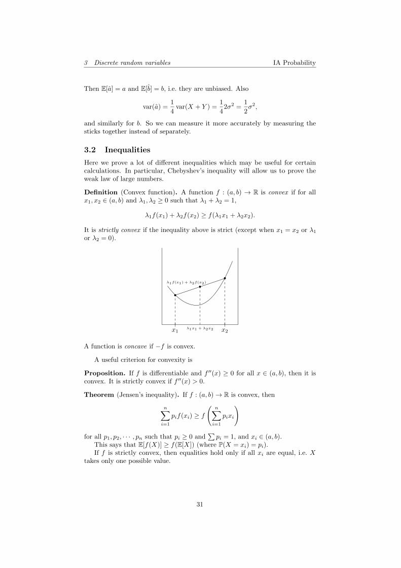
Definition (Convex function). A function f : (a, b) → R is convex if for allx1, x2 ∈ (a, b) and λ1, λ2 ≥ 0 such that λ1 + λ2 = 1,
λ1f(x1) + λ2f(x2) ≥ f(λ1x1 + λ2x2).
It is strictly convex if the inequality above is strict (except when x1 = x2 or λ1
or λ2 = 0).
x1 x2λ1x1 + λ2x2
λ1f(x1) + λ2f(x2)
A function is concave if −f is convex.
A useful criterion for convexity is
Proposition. If f is differentiable and f ′′(x) ≥ 0 for all x ∈ (a, b), then it isconvex. It is strictly convex if f ′′(x) > 0.
Theorem (Jensen’s inequality). If f : (a, b)→ R is convex, then
n∑i=1
pif(xi) ≥ f
(n∑i=1
pixi
)
for all p1, p2, · · · , pn such that pi ≥ 0 and∑pi = 1, and xi ∈ (a, b).
This says that E[f(X)] ≥ f(E[X]) (where P(X = xi) = pi).If f is strictly convex, then equalities hold only if all xi are equal, i.e. X
takes only one possible value.
31
3 Discrete random variables IA Probability
Proof. Induct on n. It is true for n = 2 by the definition of convexity. Then
f(p1x1 + · · ·+ pnxn) = f
(p1x1 + (p2 + · · ·+ pn)
p2x2 + · · ·+ lnxnp2 + · · ·+ pn
)≤ p1f(x1) + (p2 + · · · pn)f
(p2x2 + · · ·+ pnxnp2 + · · ·+ pn
).
≤ p1f(x1) + (p2 + · · ·+ pn)
[p2
( )f(x2) + · · ·+ pn
( )f(xn)
]= p1f(x1) + · · ·+ pn(xn).
where the ( ) is p2 + · · ·+ pn.Strictly convex case is proved with ≤ replaced by < by definition of strict
convexity.
Corollary (AM-GM inequality). Given x1, · · · , xn positive reals, then(∏xi
)1/n
≤ 1
n
∑xi.
Proof. Take f(x) = − log x. This is concave since its second derivative isx−2 > 0.
Take P(x = xi) = 1/n. Then
E[f(x)] =1
n
∑− log xi = − log GM
and
f(E[x]) = − log1
n
∑xi = − log AM
Since f(E[x]) ≤ E[f(x)], AM ≥ GM. Since − log x is strictly convex, AM = GMonly if all xi are equal.
Theorem (Cauchy-Schwarz inequality). For any two random variables X,Y ,
(E[XY ])2 ≤ E[X2]E[Y 2].
Proof. If Y = 0, then both sides are 0. Otherwise, E[Y 2] > 0. Let
w = X − Y · E[XY ]
E[Y 2].
Then
E[w2] = E[X2 − 2XY
E[XY ]
E[Y 2]+ Y 2 (E[XY ])2
(E[Y 2])2
]= E[X2]− 2
(E[XY ])2
E[Y 2]+
(E[XY ])2
E[Y 2]
= E[X2]− (E[XY ])2
E[Y 2]
Since E[w2] ≥ 0, the Cauchy-Schwarz inequality follows.
32
3 Discrete random variables IA Probability
Theorem (Markov inequality). If X is a random variable with E|X| <∞ andε > 0, then
P(|X| ≥ ε) ≤ E|X|ε
.
Proof. We make use of the indicator function. We have
I[|X| ≥ ε] ≤ |X|ε.
This is proved by exhaustion: if |X| ≥ ε, then LHS = 1 and RHS ≥ 1; If |X| < ε,then LHS = 0 and RHS is non-negative.
Take the expected value to obtain
P(|X| ≥ ε) ≤ E|X|ε
.
Similarly, we have
Theorem (Chebyshev inequality). If X is a random variable with E[X2] <∞and ε > 0, then
P(|X| ≥ ε) ≤ E[X2]
ε2.
Proof. Again, we have
I[|X| ≥ ε] ≤ x2
ε2.
Then take the expected value and the result follows.
Note that these are really powerful results, since they do not make anyassumptions about the distribution of X. On the other hand, if we knowsomething about the distribution, we can often get a larger bound.
An important corollary is that if µ = E[X], then
P(|X − µ| ≥ ε) ≤ E[(X − µ)2]
ε2=
varX
ε2
3.3 Weak law of large numbers
Theorem (Weak law of large numbers). Let X1, X2, · · · be iid random variables,with mean µ and varσ2.
Let Sn =∑ni=1Xi.
Then for all ε > 0,
P(∣∣∣∣Snn − µ
∣∣∣∣ ≥ ε)→ 0
as n→∞.We say, Sn
n tends to µ (in probability), or
Snn→p µ.
33
3 Discrete random variables IA Probability
Proof. By Chebyshev,
P(∣∣∣∣Snn − µ
∣∣∣∣ ≥ ε) ≤ E(Snn − µ
)2ε2
=1
n2
E(Sn − nµ)2
ε2
=1
n2ε2var(Sn)
=n
n2ε2var(X1)
=σ2
nε2→ 0
Note that we cannot relax the “independent” condition. For example, ifX1 = X2 = X3 = · · · = 1 or 0, each with probability 1/2. Then Sn/n 6→ 1/2since it is either 1 or 0.
Example. Suppose we toss a coin with probability p of heads. Then
Snn
=number of heads
number of tosses.
Since E[Xi] = p, then the weak law of large number tells us that
Snn→p p.
This means that as we toss more and more coins, the proportion of heads willtend towards p.
Since we called the above the weak law, we also have the strong law, whichis a stronger statement.
Theorem (Strong law of large numbers).
P(Snn→ µ as n→∞
)= 1.
We saySnn→as µ,
where “as” means “almost surely”.
It can be shown that the weak law follows from the strong law, but not theother way round. The proof is left for Part II because it is too hard.
3.4 Multiple random variables
If we have two random variables, we can study the relationship between them.
Definition (Covariance). Given two random variables X,Y , the covariance is
cov(X,Y ) = E[(X − E[X])(Y − E[Y ])].
34
3 Discrete random variables IA Probability
Proposition.
(i) cov(X, c) = 0 for constant c.
(ii) cov(X + c, Y ) = cov(X,Y ).
(iii) cov(X,Y ) = cov(Y,X).
(iv) cov(X,Y ) = E[XY ]− E[X]E[Y ].
(v) cov(X,X) = var(X).
(vi) var(X + Y ) = var(X) + var(Y ) + 2 cov(X,Y ).
(vii) If X, Y are independent, cov(X,Y ) = 0.
These are all trivial to prove and proof is omitted.It is important to note that cov(X,Y ) = 0 does not imply X and Y are
independent.
Example.
– Let (X,Y ) = (2, 0), (−1,−1) or (−1, 1) with equal probabilities of 1/3.These are not independent since Y = 0⇒ X = 2.
However, cov(X,Y ) = E[XY ]− E[X]E[Y ] = 0− 0 · 0 = 0.
– If we randomly pick a point on the unit circle, and let the coordinates be(X,Y ), then E[X] = E[Y ] = E[XY ] = 0 by symmetry. So cov(X,Y ) = 0but X and Y are clearly not independent (they have to satisfy x2 +y2 = 1).
The covariance is not that useful in measuring how well two variables correlate.For one, the covariance can (potentially) have dimensions, which means that thenumerical value of the covariance can depend on what units we are using. Also,the magnitude of the covariance depends largely on the variance of X and Ythemselves. To solve these problems, we define
Definition (Correlation coefficient). The correlation coefficient of X and Y is
corr(X,Y ) =cov(X,Y )√
var(X) var(Y ).
Proposition. | corr(X,Y )| ≤ 1.
Proof. Apply Cauchy-Schwarz to X − E[X] and Y − E[Y ].
Again, zero correlation does not necessarily imply independence.Alternatively, apart from finding a fixed covariance or correlation number,
we can see how the distribution of X depends on Y . Given two random variablesX,Y , P(X = x, Y = y) is known as the joint distribution. From this jointdistribution, we can retrieve the probabilities P(X = x) and P(Y = y). We canalso consider different conditional expectations.
35
3 Discrete random variables IA Probability
Definition (Conditional distribution). Let X and Y be random variables (ingeneral not independent) with joint distribution P(X = x, Y = y). Then themarginal distribution (or simply distribution) of X is
P(X = x) =∑y∈Ωy
P(X = x, Y = y).
The conditional distribution of X given Y is
P(X = x | Y = y) =P(X = x, Y = y)
P(Y = y).
The conditional expectation of X given Y is
E[X | Y = y] =∑x∈ΩX
xP(X = x | Y = y).
We can view E[X | Y ] as a random variable in Y : given a value of Y , we returnthe expectation of X.
Example. Consider a dice roll. Let Y = 1 denote an even roll and Y = 0 denotean odd roll. Let X be the value of the roll. Then E[X | Y ] = 3 + Y , ie 4 if even,3 if odd.
Example. Let X1, · · · , Xn be iid B(1, p). Let Y = X1 + · · ·+Xn. Then
P(X1 = 1 | Y = r) =P(X1 = 1,
∑n2 Xi = r − 1)
P(Y = r)
=p(n−1r−1
)pr−1(1− p)(n−1)−(r−1)(nr
)pr(1− p)n−1
=r
n.
So
E[X1 | Y ] = 1 · rn
+ 0(
1− r
n
)=r
n=Y
n.
Note that this is a random variable!
Theorem. If X and Y are independent, then
E[X | Y ] = E[X]
Proof.
E[X | Y = y] =∑x
xP(X = x | Y = y)
=∑x
xP(X = x)
= E[X]
We know that the expected value of a dice roll given it is even is 4, and theexpected value given it is odd is 3. Since it is equally likely to be even or odd,the expected value of the dice roll is 3.5. This is formally captured by
36
3 Discrete random variables IA Probability
Theorem (Tower property of conditional expectation).
EY [EX [X | Y ]] = EX [X],
where the subscripts indicate what variable the expectation is taken over.
Proof.
EY [EX [X | Y ]] =∑y
P(Y = y)E[X | Y = y]
=∑y
P(Y = y)∑x
xP(X = x | Y = y)
=∑x
∑y
xP(X = x, Y = y)
=∑x
x∑y
P(X = x, Y = y)
=∑x
xP(X = x)
= E[X].
This is also called the law of total expectation. We can also state it as:suppose A1, A2, · · · , An is a partition of Ω. Then
E[X] =∑
i:P(Ai)>0
E[X | Ai]P(Ai).
3.5 Probability generating functions
Consider a random variable X, taking values 0, 1, 2, · · · . Let pr = P(X = r).
Definition (Probability generating function (pgf)). The probability generatingfunction (pgf) of X is
p(z) = E[zX ] =
∞∑r=0
P(X = r)zr = p0 + p1z + p2z2 · · · =
∞∑0
przr.
This is a power series (or polynomial), and converges if |z| ≤ 1, since
|p(z)| ≤∑r
pr|zr| ≤∑r
pr = 1.
We sometimes write as pX(z) to indicate what the random variable.
This definition might seem a bit out of the blue. However, it turns out to bea rather useful algebraic tool that can concisely summarize information aboutthe probability distribution.
Example. Consider a fair di.e. Then pr = 1/6 for r = 1, · · · , 6. So
p(z) = E[zX ] =1
6(z + z2 + · · ·+ z6) =
1
6z
(1− z6
1− z
).
37
3 Discrete random variables IA Probability
Theorem. The distribution of X is uniquely determined by its probabilitygenerating function.
Proof. By definition, p0 = p(0), p1 = p′(0) etc. (where p′ is the derivative of p).In general,
di
dzip(z)
∣∣∣∣z=0
= i!pi.
So we can recover (p0, p1, · · · ) from p(z).
Theorem (Abel’s lemma).
E[X] = limz→1
p′(z).
If p′(z) is continuous, then simply E[X] = p′(1).
Note that this theorem is trivial if p′(1) exists, as long as we know that wecan differentiate power series term by term. What is important here is that evenif p′(1) doesn’t exist, we can still take the limit and obtain the expected value,e.g. when E[X] =∞.
Proof. For z < 1, we have
p′(z) =
∞∑1
rprzr−1 ≤
∞∑1
rpr = E[X].
So we must havelimz→1
p′(z) ≤ E[X].
On the other hand, for any ε, if we pick N large, then
N∑1
rpr ≥ E[X]− ε.
So
E[X]− ε ≤N∑1
rpr = limz→1
N∑1
rprzr−1 ≤ lim
z→1
∞∑1
rprzr−1 = lim
z→1p′(z).
So E[X] ≤ limz→1
p′(z). So the result follows
Theorem.E[X(X − 1)] = lim
z→1p′′(z).
Proof. Same as above.
Example. Consider the Poisson distribution. Then
pr = P(X = r) =1
r!λre−λ.
Then
p(z) = E[zX ] =∞∑0
zr1
r!λre−λ = eλze−λ = eλ(z−1).
38
3 Discrete random variables IA Probability
We can have a sanity check: p(1) = 1, which makes sense, since p(1) is the sumof probabilities.
We have
E[X] =d
dzeλ(z−1)
∣∣∣∣z=1
= λ,
and
E[X(X − 1)] =d2
dx2eλ(z−1)
∣∣∣∣z=1
= λ2
Sovar(X) = E[X2]− E[X]2 = λ2 + λ− λ2 = λ.
Theorem. Suppose X1, X2, · · · , Xn are independent random variables with pgfsp1, p2, · · · , pn. Then the pgf of X1 +X2 + · · ·+Xn is p1(z)p2(z) · · · pn(z).
Proof.
E[zX1+···+Xn ] = E[zX1 · · · zXn ] = E[zX1 ] · · ·E[zXn ] = p1(z) · · · pn(z).
Example. Let X ∼ B(n, p). Then
p(z) =
n∑r=0
P(X = r)zr =∑(
n
r
)pr(1− p)n−rzr = (pz+ (1− p))n = (pz+ q)n.
So p(z) is the product of n copies of pz+ q. But pz+ q is the pgf of Y ∼ B(1, p).This shows that X = Y1 + Y2 + · · · + Yn (which we already knew), i.e. a
binomial distribution is the sum of Bernoulli trials.
Example. If X and Y are independent Poisson random variables with parame-ters λ, µ respectively, then
E[tX+Y ] = E[tX ]E[tY ] = eλ(t−1)eµ(t−1) = e(λ+µ)(t−1)
So X + Y ∼ P(λ+ µ).We can also do it directly:
P(X + Y = r) =
r∑i=0
P(X = i, Y = r − i) =
r∑i=0
P(X = i)P(X = r − i),
but is much more complicated.
We can use pgf-like functions to obtain some combinatorial results.
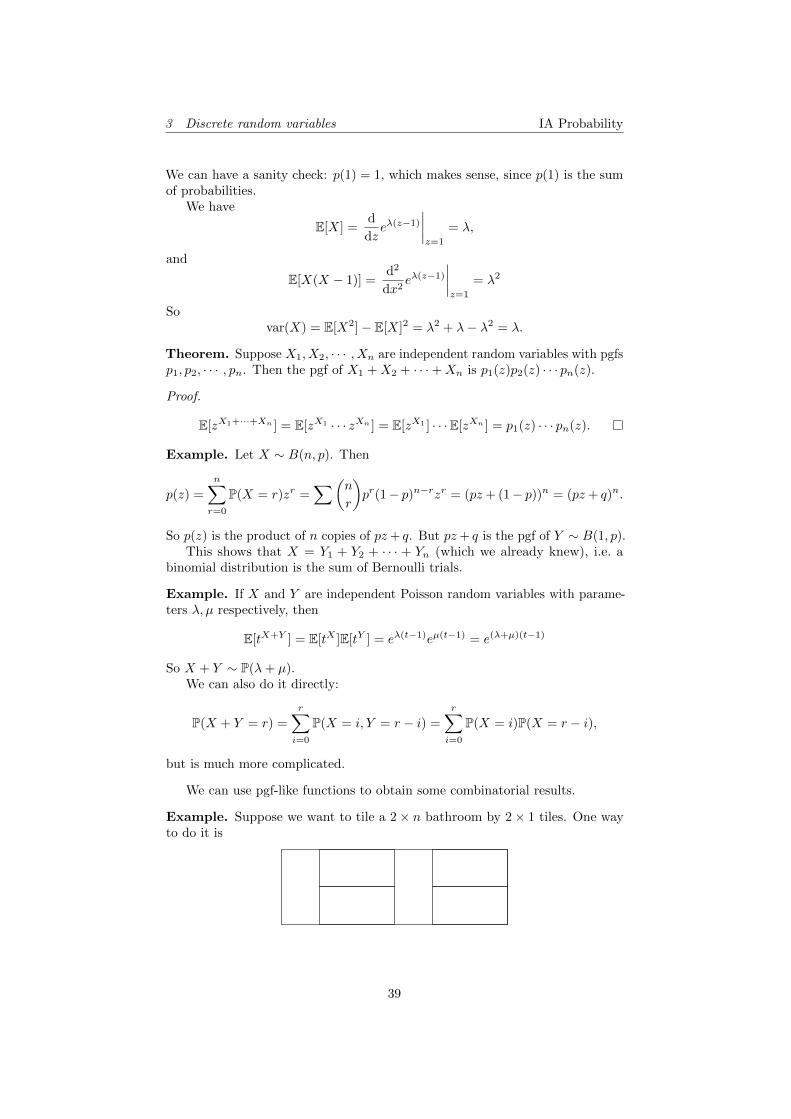
Example. Suppose we want to tile a 2× n bathroom by 2× 1 tiles. One wayto do it is
39
3 Discrete random variables IA Probability
We can do it recursively: suppose there are fn ways to tile a 2× n grid. Then ifwe start tiling, the first tile is either vertical, in which we have fn−1 ways to tilethe remaining ones; or the first tile is horizontal, in which we have fn−2 ways totile the remaining. So
fn = fn−1 + fn−2,
which is simply the Fibonacci sequence, with f0 = f1 = 1.Let
F (z) =
∞∑n=0
fnzn.
Then from our recurrence relation, we obtain
fnzn = fn−1z
n + fn−2zn.
So∞∑n=2
fnzn =
∞∑n=2
fn−1zn +
∞∑n=2
fn−2zn.
Since f0 = f1 = 1, we have
F (z)− f0 − zf1 = z(F (z)− f0) + z2F (z).
Thus F (z) = (1− z − z2)−1. If we write
α1 =1
2(1 +
√5), α2 =
1
2(1−
√5).
then we have
F (z) = (1− z − z2)−1
=1
(1− α1z)(1− α2z)
=1
α1 − α2
(α1
1− α1z− α2
1− α2z
)=
1
α1 − α2
(α1
∞∑n=0
αn1 zn − α2
∞∑n=0
αn2 zn
).
So
fn =αn+1
1 − αn+12
α1 − α2.
Example. A Dyck word is a string of brackets that match, such as (), or ((())()).There is only one Dyck word of length 2, (). There are 2 of length 4, (()) and
()(). Similarly, there are 5 Dyck words of length 5.Let Cn be the number of Dyck words of length 2n. We can split each Dyck
word into (w1)w2, where w1 and w2 are Dyck words. Since the lengths of w1
and w2 must sum up to 2(n− 1),
Cn+1 =
n∑i=0
CiCn−i. (∗)
40
3 Discrete random variables IA Probability
We again use pgf-like functions: let
c(x) =
∞∑n=0
Cnxn.
From (∗), we can show that
c(x) = 1 + xc(x)2.
We can solve to show that
c(x) =1−√
1− 4x
2x=
∞∑0
(2n
n
)xn
n+ 1,
noting that C0 = 1. Then
Cn =1
n+ 1
(2n
n
).
Sums with a random number of terms
A useful application of generating functions is the sum with a random numberof random terms. For example, an insurance company may receive a randomnumber of claims, each demanding a random amount of money. Then we havea sum of a random number of terms. This can be answered using probabilitygenerating functions.
Example. Let X1, X2, · · · , Xn be iid with pgf p(z) = E[zX ]. Let N be a randomvariable independent of Xi with pgf h(z). What is the pgf of S = X1 + · · ·+XN?
E[zS ] = E[zX1+···+XN ]
= EN [EXi [zX1+...+XN | N ]︸ ︷︷ ︸assuming fixed N
]
=
∞∑n=0
P(N = n)E[zX1+X2+···+Xn ]
=
∞∑n=0
P(N = n)E[zX1 ]E[zX2 ] · · ·E[zXn ]
=
∞∑n=0
P(N = n)(E[zX1 ])n
=
∞∑n=0
P(N = n)p(z)n
= h(p(z))
since h(x) =∑∞n=0 P(N = n)xn.
So
E[S] =d
dzh(p(z))
∣∣∣∣z=1
= h′(p(1))p′(1)
= E[N ]E[X1]
41
3 Discrete random variables IA Probability
To calculate the variance, use the fact that
E[S(S − 1)] =d2
dz2h(p(z))
∣∣∣∣z=1
.
Then we can find that
var(S) = E[N ] var(X1) + E[X21 ] var(N).
42
4 Interesting problems IA Probability
4 Interesting problems
Here we are going to study two rather important and interesting probabilisticprocesses — branching processes and random walks. Solutions to these willtypically involve the use of probability generating functions.
4.1 Branching processes
Branching processes are used to model population growth by reproduction. Atthe beginning, there is only one individual. At each iteration, the individualproduces a random number of offsprings. In the next iteration, each offspringwill individually independently reproduce randomly according to the samedistribution. We will ask questions such as the expected number of individualsin a particular generation and the probability of going extinct.
Consider X0, X1, · · · , where Xn is the number of individuals in the nthgeneration. We assume the following:
(i) X0 = 1
(ii) Each individual lives for unit time and produces k offspring with probabilitypk.
(iii) Suppose all offspring behave independently. Then
Xn+1 = Y n1 + Y n2 + · · ·+ Y nXn ,
where Y ni are iid random variables, which is the same as X1 (the superscriptdenotes the generation).
It is useful to consider the pgf of a branching process. Let F (z) be the pgf ofY ni . Then
F (z) = E[zYni ] = E[zX1 ] =
∞∑k=0
pkzk.
DefineFn(z) = E[zXn ].
The main theorem of branching processes here is
Theorem.
Fn+1(z) = Fn(F (z)) = F (F (F (· · ·F (z) · · · )))) = F (Fn(z)).
43
4 Interesting problems IA Probability
Proof.
Fn+1(z) = E[zXn+1 ]
= E[E[zXn+1 | Xn]]
=
∞∑k=0
P(Xn = k)E[zXn+1 | Xn = k]
=
∞∑k=0
P(Xn = k)E[zYn1 +···+Y nk | Xn = k]
=
∞∑k=0
P(Xn = k)E[zY1 ]E[zY2 ] · · ·E[zYn ]
=
∞∑k=0
P(Xn = k)(E[zX1 ])k
=∑k=0
P(Xn = k)F (z)k
= Fn(F (z))
Theorem. Suppose
E[X1] =∑
kpk = µ
andvar(X1) = E[(X − µ)2] =
∑(k − µ)2pk <∞.
ThenE[Xn] = µn, varXn = σ2µn−1(1 + µ+ µ2 + · · ·+ µn−1).
Proof.
E[Xn] = E[E[Xn | Xn−1]]
= E[µXn−1]
= µE[Xn−1]
Then by induction, E[Xn] = µn (since X0 = 1).To calculate the variance, note that
var(Xn) = E[X2n]− (E[Xn])2
and henceE[X2
n] = var(Xn) + (E[X])2
We then calculate
E[X2n] = E[E[X2
n | Xn−1]]
= E[var(Xn) + (E[Xn])2 | Xn−1]
= E[Xn−1 var(X1) + (µXn−1)2]
= E[Xn−1σ2 + (µXn−1)2]
= σ2µn−1 + µ2E[X2n−1].
44
4 Interesting problems IA Probability
So
varXn = E[X2n]− (E[Xn])2
= µ2E[X2n−1] + σ2µn−1 − µ2(E[Xn−1])2
= µ2(E[X2n−1]− E[Xn−1]2) + σ2µn−1
= µ2 var(Xn−1) + σ2µn−1
= µ4 var(Xn−2) + σ2(µn−1 + µn)
= · · ·= µ2(n−1) var(X1) + σ2(µn−1 + µn + · · ·+ µ2n−3)
= σ2µn−1(1 + µ+ · · ·+ µn−1).
Of course, we can also obtain this using the probability generating function aswell.
Extinction probability
Let An be the event Xn = 0, ie extinction has occurred by the nth generation.Let q be the probability that extinction eventually occurs. Let
A =
∞⋃n=1
An = [extinction eventually occurs].
Since A1 ⊆ A2 ⊆ A3 ⊆ · · · , we know that
q = P(A) = limn→∞
P(An) = limn→∞
P(Xn = 0).
ButP(Xn = 0) = Fn(0),
since Fn(0) =∑
P(Xn = k)zk. So
F (q) = F(
limn→∞
Fn(0))
= limn→∞
F (Fn(0)) = limn→∞
Fn+1(0) = q.
SoF (q) = q.
Alternatively, using the law of total probability
q =∑k
P(X1 = k)P(extinction | X1 = k) =∑k
pkqk = F (q),
where the second equality comes from the fact that for the whole population togo extinct, each individual population must go extinct.
This means that to find the probability of extinction, we need to find a fixedpoint of F . However, if there are many fixed points, which should we pick?
Theorem. The probability of extinction q is the smallest root to the equationq = F (q). Write µ = E[X1]. Then if µ ≤ 1, then q = 1; if µ > 1, then q < 1.
45
4 Interesting problems IA Probability
Proof. To show that it is the smallest root, let α be the smallest root. Then notethat 0 ≤ α⇒ F (0) ≤ F (α) = α since F is increasing (proof: write the functionout!). Hence F (F (0)) ≤ α. Continuing inductively, Fn(0) ≤ α for all n. So
q = limn→∞
Fn(0) ≤ α.
So q = α.To show that q = 1 when µ ≤ 1, we show that q = 1 is the only root. We
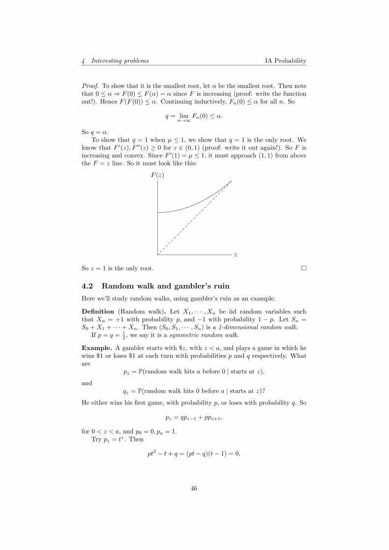
know that F ′(z), F ′′(z) ≥ 0 for z ∈ (0, 1) (proof: write it out again!). So F isincreasing and convex. Since F ′(1) = µ ≤ 1, it must approach (1, 1) from abovethe F = z line. So it must look like this:
z
F (z)
So z = 1 is the only root.
4.2 Random walk and gambler’s ruin
Here we’ll study random walks, using gambler’s ruin as an example.
Definition (Random walk). Let X1, · · · , Xn be iid random variables suchthat Xn = +1 with probability p, and −1 with probability 1 − p. Let Sn =S0 +X1 + · · ·+Xn. Then (S0, S1, · · · , Sn) is a 1-dimensional random walk.
If p = q = 12 , we say it is a symmetric random walk.
Example. A gambler starts with $z, with z < a, and plays a game in which hewins $1 or loses $1 at each turn with probabilities p and q respectively. Whatare
pz = P(random walk hits a before 0 | starts at z),
andqz = P(random walk hits 0 before a | starts at z)?
He either wins his first game, with probability p, or loses with probability q. So
pz = qpz−1 + ppz+1,
for 0 < z < a, and p0 = 0, pa = 1.Try pz = tz. Then
pt2 − t+ q = (pt− q)(t− 1) = 0,
46
4 Interesting problems IA Probability
noting that p = 1− q. If p 6= q, then
pz = A1z +B
(q
p
)z.
Since pz = 0, we get A = −B. Since pa = 1, we obtain
pz =1− (p/q)z
1− (p/q)a.
If p = q, then pz = A+Bz = z/a.Similarly, (or perform the substitutions p 7→ q, q 7→ p and z 7→ a− z)
qz =(p/q)z − (q/p)a
1− (p/q)a
if p 6= q, and
qz =a− zz
if p = q. Since pz + qz = 1, we know that the game will eventually end.What if a→∞? What is the probability of going bankrupt?
P(path hits 0 ever) = P
( ∞⋃a=z+1
[path hits 0 before a]
)= lima→∞
P(path hits 0 before a)
= lima→∞
qz
=
(p/q)z p > q
1 p ≤ q.
So if the odds are against you (i.e. the probability of losing is greater than theprobability of winning), then no matter how small the difference is, you arebound to going bankrupt eventually.
Duration of the game
Let Dz = expected time until the random walk hits 0 or a, starting from z. Wefirst show that this is bounded. We know that there is one simple way to hit 0or a: get +1 or −1 for a times in a row. This happens with probability pa + qa,and takes a steps. So even if this were the only way to hit 0 or a, the expectedduration would be a
pa+qa . So we must have
Dz ≤a
pa + qa
This is a very crude bound, but it is sufficient to show that it is bounded, andwe can meaningfully apply formulas to this finite quantity.
We have
Dz = E[duration]
= E[E[duration | X1]]
= pE[duration | X1 = 1] + qE[duration | X1 = −1]
= p(1 +Dz+1) + q(1−Dz−1)
47
4 Interesting problems IA Probability
SoDz = 1 + pDz+1 + qDz−1,
subject to D0 = Da = 0.We first find a particular solution by trying Dz = Cz. Then
Cz = 1 + pC(z + 1) = qC(z − 1).
So
C =1
q − p,
for p 6= q. The we find the complementary solution. Try Dz = tz.
pt2 − t+ q = 0,
which has roots 1 and q/p. So the general solution is
Dz = A+B
(q
p
)z+
z
q − p.
Putting in the boundary conditions,
Dz =z
q − p− a
q − p· 1− (q/p)z
1− (q/p)a.
If p = q, then to find the particular solution, we have to try
Dz = Cz2.
Then we find C = −1. So
Dz = −z2 +A+Bz.
Then the boundary conditions give
Dz = z(a− z).
Using generating functions
We can use generating functions to solve the problem as well.Let Uz,n = P(random walk absorbed at 0 at n | start in z).We have the following conditions: U0,0 = 1; Uz,0 = 0 for 0 < z ≤ a;
U0,n = Ua,n = 0 for n > 0.We define a pgf-like function.
Uz(s) =
∞∑n=0
Uz,nsn.
We know thatUz,n+1 = pUz+1,n + qUz−1,n.
Multiply by sn+1 and sum on n = 0, 1, · · · . Then
Uz(s) = psUz+1(s) + qsUz−1(s).
48
4 Interesting problems IA Probability
We try Uz(s) = [λ(s)]z. Then
λ(s) = psλ(s)2 + qs.
Then
λ1(s), λ2(s) =1±
√1− 4pqs2
2ps.
SoUz(s) = A(s)λ1(s)z +B(s)λ2(s)z.
Since U0(s) = 1 and Ua(s) = 0, we know that
A(s) +B(s) = 1
andA(s)λ1(s)a +B(s)λ2(s)a = 0.
Then we find that
Uz(s) =λ1(s)aλ2(s)z − λ2(s)aλ1(s)z
λ1(s)a − λ2(s)a.
Since λ1(s)λ2(s) = qp , we can “simplify” this to obtain
Uz(s) =
(q
p
)z· λ1(s)a−z − λ2(s)a−z
λ1(s)a − λ2(s)a.
We see that Uz(1) = qz. We can apply the same method to find the generatingfunction for absorption at a, say Vz(s). Then the generating function for theduration is Uz + Vz. Hence the expected duration is Dz = U ′z(1) + V ′z (1).
49
5 Continuous random variables IA Probability
5 Continuous random variables
5.1 Continuous random variables
So far, we have only looked at the case where the outcomes Ω are discrete.Consider an experiment where we throw a needle randomly onto the groundand record the angle it makes with a fixed horizontal. Then our sample space isΩ = ω ∈ R : 0 ≤ ω < 2π. Then we have
P(ω ∈ [0, θ]) =θ
2π, 0 ≤ θ ≤ 2π.
With continuous distributions, we can no longer talk about the probability ofgetting a particular number, since this is always zero. For example, we willalmost never get an angle of exactly 0.42 radians.
Instead, we can only meaningfully talk about the probability of X falling intoa particular range. To capture the distribution of X, we want to define a functionf such that for each x and small δx, the probability of X lying in [x, x+ δx] isgiven by f(x)δx + o(δx). This f is known as the probability density function.
Integrating this, we know that the probability of X ∈ [a, b] is∫ baf(x) dx. We
take this as the definition of f .
Definition (Continuous random variable). A random variable X : Ω → R iscontinuous if there is a function f : R→ R≥0 such that
P(a ≤ X ≤ b) =
∫ b
a
f(x) dx.
We call f the probability density function, which satisfies
– f ≥ 0
–∫∞−∞ f(x) = 1.
Note that P(X = a) = 0 since it is∫ aaf(x) dx. Then we also have
P
⋃a∈Q
[X = a]
= 0,
since it is a countable union of probability 0 events (and axiom 3 states that theprobability of the countable union is the sum of probabilities, i.e. 0).
Definition (Cumulative distribution function). The cumulative distributionfunction (or simply distribution function) of a random variable X (discrete,continuous, or neither) is
F (x) = P(X ≤ x).
We can see that F (x) is increasing and F (x)→ 1 as x→∞.In the case of continuous random variables, we have
F (x) =
∫ x
∞f(z) dz.
50
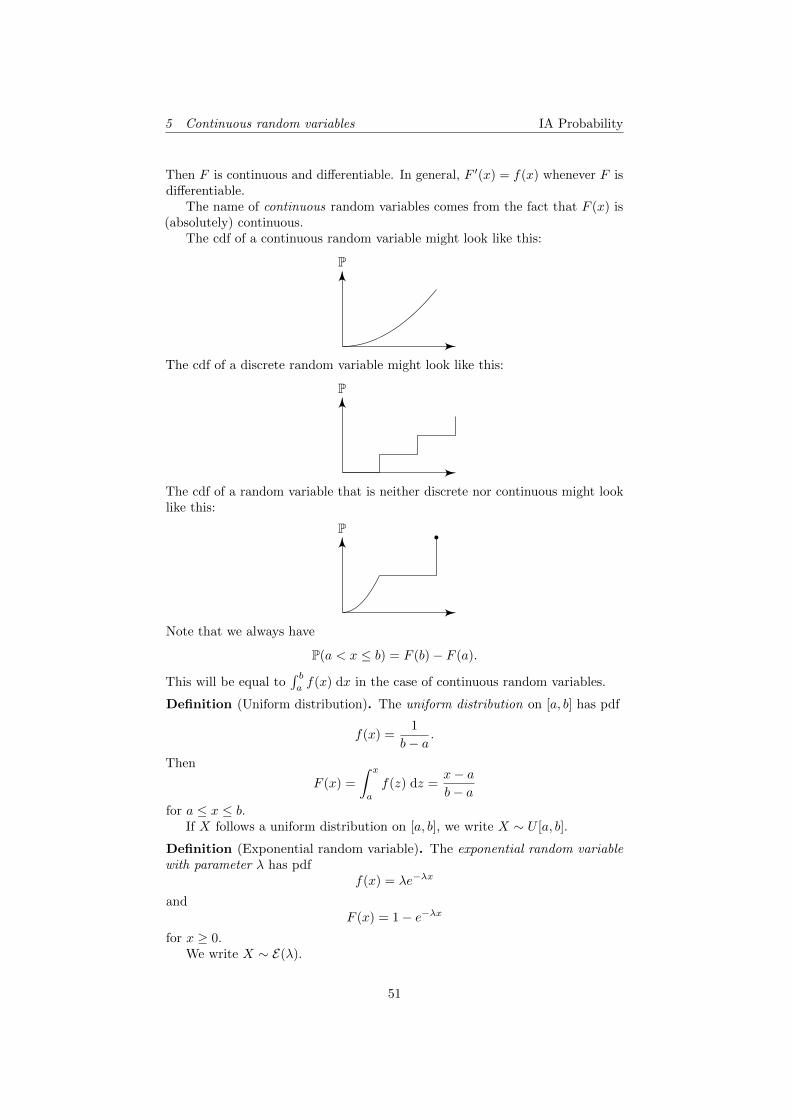
5 Continuous random variables IA Probability
Then F is continuous and differentiable. In general, F ′(x) = f(x) whenever F isdifferentiable.
The name of continuous random variables comes from the fact that F (x) is(absolutely) continuous.
The cdf of a continuous random variable might look like this:
P
The cdf of a discrete random variable might look like this:
P
The cdf of a random variable that is neither discrete nor continuous might looklike this:
P
Note that we always have
P(a < x ≤ b) = F (b)− F (a).
This will be equal to∫ baf(x) dx in the case of continuous random variables.
Definition (Uniform distribution). The uniform distribution on [a, b] has pdf
f(x) =1
b− a.
Then
F (x) =
∫ x
a
f(z) dz =x− ab− a
for a ≤ x ≤ b.If X follows a uniform distribution on [a, b], we write X ∼ U [a, b].
Definition (Exponential random variable). The exponential random variablewith parameter λ has pdf
f(x) = λe−λx
andF (x) = 1− e−λx
for x ≥ 0.We write X ∼ E(λ).
51
5 Continuous random variables IA Probability
Then
P(a ≤ x ≤ b) =
∫ b
a
f(z) dz = e−λa − e−λb.
Proposition. The exponential random variable is memoryless, i.e.
P(X ≥ x+ z | X ≥ x) = P(X ≥ z).
This means that, say if X measures the lifetime of a light bulb, knowing it hasalready lasted for 3 hours does not give any information about how much longerit will last.
Recall that the geometric random variable is the discrete memoryless randomvariable.
Proof.
P(X ≥ x+ z | X ≥ x) =P(X ≥ x+ z)
P(X ≥ x)
=
∫∞x+z
f(u) du∫∞xf(u) du
=e−λ(x+z)
e−λx
= e−λz
= P(X ≥ z).
Similarly, given that, you have lived for x days, what is the probability ofdying within the next δx days?
P(X ≤ x+ δx | X ≥ x) =P(x ≤ X ≤ x+ δx)
P(X ≥ x)
=λe−λxδx
e−λx
= λδx.
So it is independent of how old you currently are, assuming your survival followsan exponential distribution.
In general, we can define the hazard rate to be
h(x) =f(x)
1− F (x).
Then
P(x ≤ X ≤ x+ δx | X ≥ x) =P(x ≤ X ≤ x+ δx)
P(X ≥ x)=
δxf(x)
1− F (x)= δx · h(x).
In the case of exponential distribution, h(x) is constant and equal to λ.Similar to discrete variables, we can define the expected value and the variance.
However, we will (obviously) have to replace the sum with an integral.
52
5 Continuous random variables IA Probability
Definition (Expectation). The expectation (or mean) of a continuous randomvariable is
E[X] =
∫ ∞−∞
xf(x) dx,
provided not both∫∞
0xf(x) dx and
∫ 0
−∞ xf(x) dx are infinite.
Theorem. If X is a continuous random variable, then
E[X] =
∫ ∞0
P(X ≥ x) dx−∫ ∞
0
P(X ≤ −x) dx.
This result is more intuitive in the discrete case:
∞∑x=0
xP(X = x) =
∞∑x=0
∞∑y=x+1
P(X = y) =
∞∑x=0
P(X > x),
where the first equality holds because on both sides, we have x copies of P(X = x)in the sum.
Proof. ∫ ∞0
P(X ≥ x) dx =
∫ ∞0
∫ ∞x
f(y) dy dx
=
∫ ∞0
∫ ∞0
I[y ≥ x]f(y) dy dx
=
∫ ∞0
(∫ ∞0
I[x ≤ y] dx
)f(y) dy
=
∫ ∞0
yf(y) dy.
We can similarly show that∫∞
0P(X ≤ −x) dx = −
∫ 0
−∞ yf(y) dy.
Example. Suppose X ∼ E(λ). Then
P(X ≥ x) =
∫ ∞x
λe−λt dt = e−λx.
So
E[X] =
∫ ∞0
e−λx dx =1
λ.
Definition (Variance). The variance of a continuous random variable is
var(X) = E[(X − E[X])2] = E[X2]− (E[X])2.
So we have
var(X) =
∫ ∞−∞
x2f(x) dx−(∫ ∞−∞
xf(x) dx
)2
.
53
5 Continuous random variables IA Probability
Example. Let X ∼ U [a, b]. Then
E[X] =
∫ b
a
x1
b− adx =
a+ b
2.
So
var(X) =
∫ b
a
x2 1
b− adx− (E[X])2
=1
12(b− a)2.
Apart from the mean, or expected value, we can also have other notions of“average values”.
Definition (Mode and median). Given a pdf f(x), we call x a mode if
f(x) ≥ f(x)
for all x. Note that a distribution can have many modes. For example, in theuniform distribution, all x are modes.
We say it is a median if∫ x
−∞f(x) dx =
1
2=
∫ ∞x
f(x) dx.
For a discrete random variable, the median is x such that
P(X ≤ x) ≥ 1
2, P(X ≥ x) ≥ 1
2.
Here we have a non-strict inequality since if the random variable, say, alwaystakes value 0, then both probabilities will be 1.
Suppose that we have an experiment whose outcome follows the distributionof X. We can perform the experiment many times and obtain many resultsX1, · · · , Xn. The average of these results is known as the sample mean.
Definition (Sample mean). If X1, · · · , Xn is a random sample from somedistribution, then the sample mean is
X =1
n
n∑1
Xi.
5.2 Stochastic ordering and inspection paradox
We want to define a (partial) order on two different random variables. Forexample, we might want to say that X + 2 > X, where X is a random variable.
A simple definition might be expectation ordering, where X ≥ Y if E[X] ≥E[Y ]. This, however, is not satisfactory since X ≥ Y and Y ≥ X does not implyX = Y . Instead, we can use the stochastic order.
Definition (Stochastic order). The stochastic order is defined as: X ≥st Y ifP(X > t) ≥ P(Y > t) for all t.
54
5 Continuous random variables IA Probability
This is clearly transitive. Stochastic ordering implies expectation ordering,since
X ≥st Y ⇒∫ ∞
0
P(X > x) dx ≥∫ ∞
0
P(y > x) dx⇒ E[X] ≥ E[Y ].
Alternatively, we can also order things by hazard rate.
Example (Inspection paradox). Suppose that n families have children attendinga school. Family i has Xi children at the school, where X1, · · · , Xn are iid randomvariables, with P (Xi = k) = pk. Suppose that the average family size is µ.
Now pick a child at random. What is the probability distribution of hisfamily size? Let J be the index of the family from which she comes (which is arandom variable). Then
P(XJ = k | J = j) =P(J = j,Xj = k)
P(J = j).
The denominator is 1/n. The numerator is more complex. This would requirethe jth family to have k members, which happens with probability pk; andthat we picked a member from the jth family, which happens with probability
E[
kk+
∑i6=j Xi
]. So
P(XJ = k | J = j) = E
[nkpk
k +∑i 6=j Xi
].
Note that this is independent of j. So
P(XJ = k) = E
[nkpk
k +∑i 6=j Xi
].
Also, P(X1 = k) = pk. So
P(XJ = k)
P(X1 = k)= E
[nk
k +∑i6=j Xi
].
This is increasing in k, and greater than 1 for k > µ. So the average value of thefamily size of the child we picked is greater than the average family size. It canbe shown that XJ is stochastically greater than X1.
This means that if we pick the children randomly, the sample mean of thefamily size will be greater than the actual mean. This is since for the larger afamily is, the more likely it is for us to pick a child from the family.
5.3 Jointly distributed random variables
Definition (Joint distribution). Two random variables X,Y have joint distri-bution F : R2 7→ [0, 1] defined by
F (x, y) = P(X ≤ x, Y ≤ y).
The marginal distribution of X is
FX(x) = P(X ≤ x) = P(X ≤ x, Y <∞) = F (x,∞) = limy→∞
F (x, y)
55
5 Continuous random variables IA Probability
Definition (Jointly distributed random variables). We say X1, · · · , Xn arejointly distributed continuous random variables and have joint pdf f if for anyset A ⊆ Rn
P((X1, · · · , Xn) ∈ A) =
∫(x1,···xn)∈A
f(x1, · · · , xn) dx1 · · · dxn.
wheref(x1, · · · , xn) ≥ 0
and ∫Rnf(x1, · · · , xn) dx1 · · · dxn = 1.
Example. In the case where n = 2,
F (x, y) = P(X ≤ x, Y ≤ y) =
∫ x
−∞
∫ y
−∞f(x, y) dx dy.
If F is differentiable, then
f(x, y) =∂2
∂x∂yF (x, y).
Theorem. If X and Y are jointly continuous random variables, then they areindividually continuous random variables.
Proof. We prove this by showing that X has a density function.We know that
P(X ∈ A) = P(X ∈ A, Y ∈ (−∞,+∞))
=
∫x∈A
∫ ∞−∞
f(x, y) dy dx
=
∫x∈A
fX(x) dx
So
fX(x) =
∫ ∞−∞
f(x, y) dy
is the (marginal) pdf of X.
Definition (Independent continuous random variables). Continuous randomvariables X1, · · · , Xn are independent if
P(X1 ∈ A1, X2 ∈ A2, · · · , Xn ∈ An) = P(X1 ∈ A1)P(X2 ∈ A2) · · ·P(Xn ∈ An)
for all Ai ⊆ ΩXi .If we let FXi and fXi be the cdf, pdf of X, then
F (x1, · · · , xn) = FX1(x1) · · ·FXn(xn)
andf(x1, · · · , xn) = fX1(x1) · · · fXn(xn)
are each individually equivalent to the definition above.
56
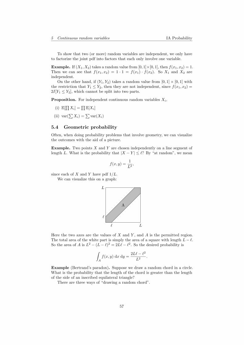
5 Continuous random variables IA Probability
To show that two (or more) random variables are independent, we only haveto factorize the joint pdf into factors that each only involve one variable.
Example. If (X1, X2) takes a random value from [0, 1]×[0, 1], then f(x1, x2) = 1.Then we can see that f(x1, x2) = 1 · 1 = f(x1) · f(x2). So X1 and X2 areindependent.
On the other hand, if (Y1, Y2) takes a random value from [0, 1]× [0, 1] withthe restriction that Y1 ≤ Y2, then they are not independent, since f(x1, x2) =2I[Y1 ≤ Y2], which cannot be split into two parts.
Proposition. For independent continuous random variables Xi,
(i) E[∏Xi] =
∏E[Xi]
(ii) var(∑Xi) =
∑var(Xi)
5.4 Geometric probability
Often, when doing probability problems that involve geometry, we can visualizethe outcomes with the aid of a picture.
Example. Two points X and Y are chosen independently on a line segment oflength L. What is the probability that |X − Y | ≤ `? By “at random”, we mean
f(x, y) =1
L2,
since each of X and Y have pdf 1/L.We can visualize this on a graph:
A
` L
`
L
Here the two axes are the values of X and Y , and A is the permitted region.The total area of the white part is simply the area of a square with length L− `.So the area of A is L2 − (L− `)2 = 2L`− `2. So the desired probability is∫
A
f(x, y) dx dy =2L`− `2
L2.
Example (Bertrand’s paradox). Suppose we draw a random chord in a circle.What is the probability that the length of the chord is greater than the lengthof the side of an inscribed equilateral triangle?
There are three ways of “drawing a random chord”.
57
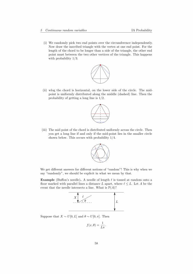
5 Continuous random variables IA Probability
(i) We randomly pick two end points over the circumference independently.Now draw the inscribed triangle with the vertex at one end point. For thelength of the chord to be longer than a side of the triangle, the other endpoint must between the two other vertices of the triangle. This happenswith probability 1/3.
(ii) wlog the chord is horizontal, on the lower side of the circle. The mid-point is uniformly distributed along the middle (dashed) line. Then theprobability of getting a long line is 1/2.
(iii) The mid point of the chord is distributed uniformly across the circle. Thenyou get a long line if and only if the mid-point lies in the smaller circleshown below. This occurs with probability 1/4.
We get different answers for different notions of “random”! This is why when wesay “randomly”, we should be explicit in what we mean by that.
Example (Buffon’s needle). A needle of length ` is tossed at random onto afloor marked with parallel lines a distance L apart, where ` ≤ L. Let A be theevent that the needle intersects a line. What is P(A)?
`Xθ L
Suppose that X ∼ U [0, L] and θ ∼ U [0, π]. Then
f(x, θ) =1
Lπ.
58
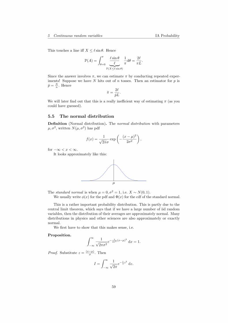
5 Continuous random variables IA Probability
This touches a line iff X ≤ ` sin θ. Hence
P(A) =
∫ π
θ=0
` sin θ
`︸ ︷︷ ︸P(X≤` sin θ)
1
πdθ =
2`
πL.
Since the answer involves π, we can estimate π by conducting repeated exper-iments! Suppose we have N hits out of n tosses. Then an estimator for p isp = N
n . Hence
π =2`
pL.
We will later find out that this is a really inefficient way of estimating π (as youcould have guessed).
5.5 The normal distribution
Definition (Normal distribution). The normal distribution with parametersµ, σ2, written N(µ, σ2) has pdf
f(x) =1√2πσ
exp
(− (x− µ)2
2σ2
),
for −∞ < x <∞.It looks approximately like this:
µ
The standard normal is when µ = 0, σ2 = 1, i.e. X ∼ N(0, 1).We usually write φ(x) for the pdf and Φ(x) for the cdf of the standard normal.
This is a rather important probability distribution. This is partly due to thecentral limit theorem, which says that if we have a large number of iid randomvariables, then the distribution of their averages are approximately normal. Manydistributions in physics and other sciences are also approximately or exactlynormal.
We first have to show that this makes sense, i.e.
Proposition. ∫ ∞−∞
1√2πσ2
e−1
2σ2(x−µ)2 dx = 1.
Proof. Substitute z = (x−µ)σ . Then
I =
∫ ∞−∞
1√2πe−
12 z
2
dz.
59
5 Continuous random variables IA Probability
Then
I2 =
∫ ∞−∞
1√2πe−x
2/2 dx
∫ ∞∞
1√2πe−y
2/2 dy
=
∫ ∞0
∫ 2π
0
1
2πe−r
2/2r dr dθ
= 1.
We also have
Proposition. E[X] = µ.
Proof.
E[X] =1√2πσ
∫ ∞−∞
xe−(x−µ)2/2σ2
dx
=1√2πσ
∫ ∞−∞
(x− µ)e−(x−µ)2/2σ2
dx+1√2πσ
∫ ∞−∞
µe−(x−µ)2/2σ2
dx.
The first term is antisymmetric about µ and gives 0. The second is just µ timesthe integral we did above. So we get µ.
Also, by symmetry, the mode and median of a normal distribution are alsoboth µ.
Proposition. var(X) = σ2.
Proof. We have var(X) = E[X2]−(E[X])2. Substitute Z = X−µσ . Then E[Z] = 0,
E[Z2] = 1σ2E[X2].
Then
var(Z) =1√2π
∫ ∞−∞
z2e−z2/2 dz
=
[− 1√
2πze−z
2/2
]∞−∞
+1√2π
∫ ∞−∞
e−z2/2 dz
= 0 + 1
= 1
So varX = σ2.
Example. UK adult male heights are normally distributed with mean 70” andstandard deviation 3”. In the Netherlands, these figures are 71” and 3”.
What is P(Y > X), where X and Y are the heights of randomly chosen UKand Netherlands males, respectively?
We have X ∼ N(70, 32) and Y ∼ N(71, 32). Then (as we will show in laterlectures) Y −X ∼ N(1, 18).
P(Y > X) = P(Y −X > 0) = P(Y −X − 1√
18>−1√
18
)= 1− Φ(−1/
√18),
since (Y−X)−1√18
∼ N(0, 1), and the answer is approximately 0.5931.
60
5 Continuous random variables IA Probability
Now suppose that in both countries, the Olympic male basketball teams areselected from that portion of male whose hight is at least above 4” above themean (which corresponds to the 9.1% tallest males of the country). What is theprobability that a randomly chosen Netherlands player is taller than a randomlychosen UK player?
For the second part, we have
P(Y > X | X ≥ 74, Y ≥ 75) =
∫ 75
x=74φX(x) dx+
∫∞x=75
∫∞y=x
φY (y)φX(x) dy dx∫∞x=74
φX(x) dx∫∞y=75
φY (y) dy,
which is approximately 0.7558. So even though the Netherlands people are onlyslightly taller, if we consider the tallest bunch, the Netherlands people will bemuch taller on average.
5.6 Transformation of random variables
We will now look at what happens when we apply a function to random variables.We first look at the simple case where there is just one variable, and then moveon to the general case where we have multiple variables and can mix themtogether.
Single random variable
Theorem. If X is a continuous random variable with a pdf f(x), and h(x)is a continuous, strictly increasing function with h−1(x) differentiable, thenY = h(X) is a random variable with pdf
fY (y) = fX(h−1(y))d
dyh−1(y).
Proof.
FY (y) = P(Y ≤ y)
= P(h(X) ≤ y)
= P(X ≤ h−1(y))
= F (h−1(y))
Take the derivative with respect to y to obtain
fY (y) = F ′Y (y) = f(h−1(y))d
dyh−1(y).
It is often easier to redo the proof than to remember the result.
Example. Let X ∼ U [0, 1]. Let Y = − logX. Then
P(Y ≤ y) = P(− logX ≤ y)
= P(X ≥ e−y)
= 1− e−y.
But this is the cumulative distribution function of E(1). So Y is exponentiallydistributed with λ = 1.
61
5 Continuous random variables IA Probability
In general, we get the following result:
Theorem. Let U ∼ U [0, 1]. For any strictly increasing distribution function F ,the random variable X = F−1U has distribution function F .
Proof.P(X ≤ x) = P(F−1(U) ≤ x) = P(U ≤ F (x)) = F (x).
This condition “strictly increasing” is needed for the inverse to exist. If it isnot, we can define
F−1(u) = infx : F (x) ≥ u, 0 < u < 1,
and the same result holds.This can also be done for discrete random variables P(X = xi) = pi by letting
X = xj if
j−1∑i=0
pi ≤ U <
j∑i=0
pi,
for U ∼ U [0, 1].
Multiple random variables
Suppose X1, X2, · · · , Xn are random variables with joint pdf f . Let
Y1 = r1(X1, · · · , Xn)
Y2 = r2(X1, · · · , Xn)
...
Yn = rn(X1, · · · , Xn).
For example, we might have Y1 = X1
X1+X2and Y2 = X1 +X2.
Let R ⊆ Rn such that P((X1, · · · , Xn) ∈ R) = 1, i.e. R is the set of all values(Xi) can take.
Suppose S is the image of R under the above transformation, and the mapR→ S is bijective. Then there exists an inverse function
X1 = s1(Y1, · · · , Yn)
X2 = s2(Y1, · · · , Yn)
...
Xn = sn(Y1, · · · , Yn).
For example, if X1, X2 refers to the coordinates of a random point in Cartesiancoordinates, Y1, Y2 might be the coordinates in polar coordinates.
Definition (Jacobian determinant). Suppose ∂si∂yj
exists and is continuous at
every point (y1, · · · , yn) ∈ S. Then the Jacobian determinant is
J =∂(s1, · · · , sn)
∂(y1, · · · , yn)= det
∂s1∂y1
· · · ∂s1∂yn
.... . .
...∂sn∂y1
· · · ∂sn∂yn
62
5 Continuous random variables IA Probability
Take A ⊆ R and B = r(A). Then using results from IA Vector Calculus, weget
P((X1, · · · , Xn) ∈ A) =
∫A
f(x1, · · · , xn) dx1 · · · dxn
=
∫B
f(s1(y1, · · · yn), s2, · · · , sn)|J | dy1 · · · dyn
= P((Y1, · · ·Yn) ∈ B).
So
Proposition. (Y1, · · · , Yn) has density
g(y1, · · · , yn) = f(s1(y1, · · · , yn), · · · sn(y1, · · · , yn))|J |
if (y1, · · · , yn) ∈ S, 0 otherwise.
Example. Suppose (X,Y ) has density
f(x, y) =
4xy 0 ≤ x ≤ 1, 0 ≤ y ≤ 1
0 otherwise
We see that X and Y are independent, with each having a density f(x) = 2x.Define U = X/Y , V = XY . Then we have X =
√UV and Y =
√V/U .
The Jacobian is
det
(∂x/∂u ∂x/∂v∂y/∂u ∂y/∂v
)= det
(12
√v/u 1
2
√u/v
− 12
√v/u3 1
2
√1/uv
)=
1
2u
Alternatively, we can find this by considering
det
(∂u/∂x ∂u/∂y∂v/∂x ∂u/∂y
)= 2u,
and then inverting the matrix. So
g(u, v) = 4√uv
√v
u
1
2u=
2v
u,
if (u, v) is in the image S, 0 otherwise. So
g(u, v) =2v
uI[(u, v) ∈ S].
Since this is not separable, we know that U and V are not independent.
In the linear case, life is easy. Suppose
Y =
Y1
...Yn
= A
X1
...Xn
= AX
Then X = A−1Y. Then ∂xi∂yj
= (A−1)ij . So |J | = |det(A−1)| = |detA|−1. So
g(y1, · · · , yn) =1
|detA|f(A−1y).
63
5 Continuous random variables IA Probability
Example. Suppose X1, X2 have joint pdf f(x1, x2). Suppose we want to findthe pdf of Y = X1 +X2. We let Z = X2. Then X1 = Y −Z and X2 = Z. Then(
YZ
)=
(1 10 1
)(X1
X2
)= AX
Then |J | = 1/|detA| = 1. Then
g(y, z) = f(y − z, z)
So
gY (y) =
∫ ∞−∞
f(y − z, z) dz =
∫ ∞−∞
f(z, y − z) dz.
If X1 and X2 are independent, f(x1, x2) = f1(x1)f2(x2). Then
g(y) =
∫ ∞−∞
f1(z)f2(y − z) dz.
Non-injective transformations
We previously discussed transformation of random variables by injective maps.What if the mapping is not? There is no simple formula for that, and we haveto work out each case individually.
Example. Suppose X has pdf f . What is the pdf of Y = |X|?We use our definition. We have
P(|X| ∈ x(a, b)) =
∫ b
a
f(x) +
∫ −a−b
f(x) dx =
∫ b
a
(f(x) + f(−x)) dx.
SofY (x) = f(x) + f(−x),
which makes sense, since getting |X| = x is equivalent to getting X = x orX = −x.
Example. Suppose X1 ∼ E(λ), X2 ∼ E(µ) are independent random variables.Let Y = min(X1, X2). Then
P(Y ≥ t) = P(X1 ≥ t,X2 ≥ t)= P(X1 ≥ t)P(X2 ≥ t)= e−λte−µt
= e−(λ+µ)t.
So Y ∼ E(λ+ µ).
Given random variables, not only can we ask for the minimum of the variables,but also ask for, say, the second-smallest one. In general, we define the orderstatistics as follows:
Definition (Order statistics). Suppose that X1, · · · , Xn are some random vari-ables, and Y1, · · · , Yn is X1, · · · , Xn arranged in increasing order, i.e. Y1 ≤ Y2 ≤· · · ≤ Yn. This is the order statistics.
We sometimes write Yi = X(i).
64
5 Continuous random variables IA Probability
Assume the Xi are iid with cdf F and pdf f . Then the cdf of Yn is
P(Yn ≤ y) = P(X1 ≤ y, · · · , Xn ≤ y) = P(X1 ≤ y) · · ·P(Xn ≤ y) = F (y)n.
So the pdf of Yn isd
dyF (y)n = nf(y)F (y)n−1.
Also,P(Y1 ≥ y) = P(X1 ≥ y, · · · , Xn ≥ y) = (1− F (y))n.
What about the joint distribution of Y1, Yn?
G(y1, yn) = P(Y1 ≤ y1, Yn ≤ yn)
= P(Yn ≤ yn)− P(Y1 ≥ y1, Yn ≤ yn)
= F (yn)n − (F (yn)− F (y1))n.
Then the pdf is
∂2
∂y1∂ynG(y1, yn) = n(n− 1)(F (yn)− F (y1))n−2f(y1)f(yn).
We can think about this result in terms of the multinomial distribution. By defi-nition, the probability that Y1 ∈ [y1, y1+δ) and Yn ∈ (yn−δ, yn] is approximatelyg(y1, yn).
Suppose that δ is sufficiently small that all other n− 2 Xi’s are very unlikelyto fall into [y1, y1 + δ) and (yn − δ, yn]. Then to find the probability required,we can treat the sample space as three bins. We want exactly one Xi to fallinto the first and last bins, and n− 2 Xi’s to fall into the middle one. There are(
n1,n−2,1
)= n(n− 1) ways of doing so.
The probability of each thing falling into the middle bin is F (yn)− F (y1),and the probabilities of falling into the first and last bins are f(y1)δ and f(yn)δ.Then the probability of Y1 ∈ [y1, y1 + δ) and Yn ∈ (yn − δ, yn] is
n(n− 1)(F (yn)− F (y1))n−2f(y1)f(yn)δ2,
and the result follows.We can also find the joint distribution of the order statistics, say g, since it
is just given byg(y1, · · · yn) = n!f(y1) · · · f(yn),
if y1 ≤ y2 ≤ · · · ≤ yn, 0 otherwise. We have this formula because there are n!combinations of x1, · · · , xn that produces a given order statistics y1, · · · , yn, andthe pdf of each combination is f(y1) · · · f(yn).
In the case of iid exponential variables, we find a nice distribution for theorder statistic.
Example. Let X1, · · · , Xn be iid E(λ), and Y1, · · · , Yn be the order statistic.Let
Z1 = Y1
Z2 = Y2 − Y1
...
Zn = Yn − Yn−1.
65
5 Continuous random variables IA Probability
These are the distances between the occurrences. We can write this as a Z = AY,with
A =
1 0 0 · · · 0−1 1 0 · · · 0...
......
. . ....
0 0 0 · · · 1
Then det(A) = 1 and hence |J | = 1. Suppose that the pdf of Z1, · · · , Zn is, sayh. Then
h(z1, · · · , zn) = g(y1, · · · , yn) · 1= n!f(y1) · · · f(yn)
= n!λne−λ(y1+···+yn)
= n!λne−λ(nz1+(n−1)z2+···+zn)
=
n∏i=1
(λi)e−(λi)zn+1−i
Since h is expressed as a product of n density functions, we have
Zi ∼ E((n+ 1− i)λ).
with all Zi independent.
5.7 Moment generating functions
If X is a continuous random variable, then the analogue of the probabilitygenerating function is the moment generating function:
Definition (Moment generating function). The moment generating function ofa random variable X is
m(θ) = E[eθX ].
For those θ in which m(θ) is finite, we have
m(θ) =
∫ ∞−∞
eθxf(x) dx.
We can prove results similar to that we had for probability generatingfunctions.
We will assume the following without proof:
Theorem. The mgf determines the distribution of X provided m(θ) is finitefor all θ in some interval containing the origin.
Definition (Moment). The rth moment of X is E[Xr].
Theorem. The rth moment X is the coefficient of θr
r! in the power seriesexpansion of m(θ), and is
E[Xr] =dn
dθnm(θ)
∣∣∣∣θ=0
= m(n)(0).
66
5 Continuous random variables IA Probability
Proof. We have
eθX = 1 + θX +θ2
2!X2 + · · · .
So
m(θ) = E[eθX ] = 1 + θE[X] +θ2
2!E[X2] + · · ·
Example. Let X ∼ E(λ). Then its mgf is
E[eθX ] =
∫ ∞0
eθxλe−λx dx = λ
∫ ∞0
e−(λ−θ)x dx =λ
λ− θ,
where 0 < θ < λ. So
E[X] = m′(0) =λ
(λ− θ)2
∣∣∣∣θ=0
=1
λ.
Also,
E[X2] = m′′(0) =2λ
(λ− θ)3
∣∣∣∣θ=0
=2
λ2.
So
var(X) = E[X2]− E[X]2 =2
λ2− 1
λ2=
1
λ2.
Theorem. If X and Y are independent random variables with moment gener-ating functions mX(θ),mY (θ), then X + Y has mgf mX+Y (θ) = mX(θ)mY (θ).
Proof.
E[eθ(X+Y )] = E[eθXeθY ] = E[eθX ]E[eθY ] = mX(θ)mY (θ).
67
6 More distributions IA Probability
6 More distributions
6.1 Cauchy distribution
Definition (Cauchy distribution). The Cauchy distribution has pdf
f(x) =1
π(1 + x2)
for −∞ < x <∞.
We check that this is a genuine distribution:∫ ∞−∞
1
π(1 + x2)dx =
∫ π/2
−π/2
1
πdθ = 1
with the substitution x = tan θ. The distribution is a bell-shaped curve.
Proposition. The mean of the Cauchy distribution is undefined, while E[X2] =∞.
Proof.
E[X] =
∫ ∞0
x
π(1 + x2)dx+
∫ 0
−∞
x
π(1 + x2)dx =∞−∞
which is undefined, but E[X2] =∞+∞ =∞.
Suppose X,Y are independent Cauchy distributions. Let Z = X + Y . Then
f(z) =
∫ ∞−∞
fX(x)fY (z − x) dx
=
∫ ∞−∞
1
π2
1
(1 + x2)(1 + (z − x)2)dx
=1/2
π(1 + (z/2)2)
for all −∞ < z < ∞ (the integral can be evaluated using a tedious partialfraction expansion).
So 12Z has a Cauchy distribution. Alternatively the arithmetic mean of
Cauchy random variables is a Cauchy random variable.By induction, we can show that 1
n (X1 + · · ·+Xn) follows Cauchy distribution.This becomes a “counter-example” to things like the weak law of large numbersand the central limit theorem. Of course, this is because those theorems requirethe random variable to have a mean, which the Cauchy distribution lacks.
Example.
(i) If Θ ∼ U [−π2 ,π2 ], then X = tan θ has a Cauchy distribution. For example,
if we fire a bullet at a wall 1 meter apart at a random random angle θ, thevertical displacement follows a Cauchy distribution.
68
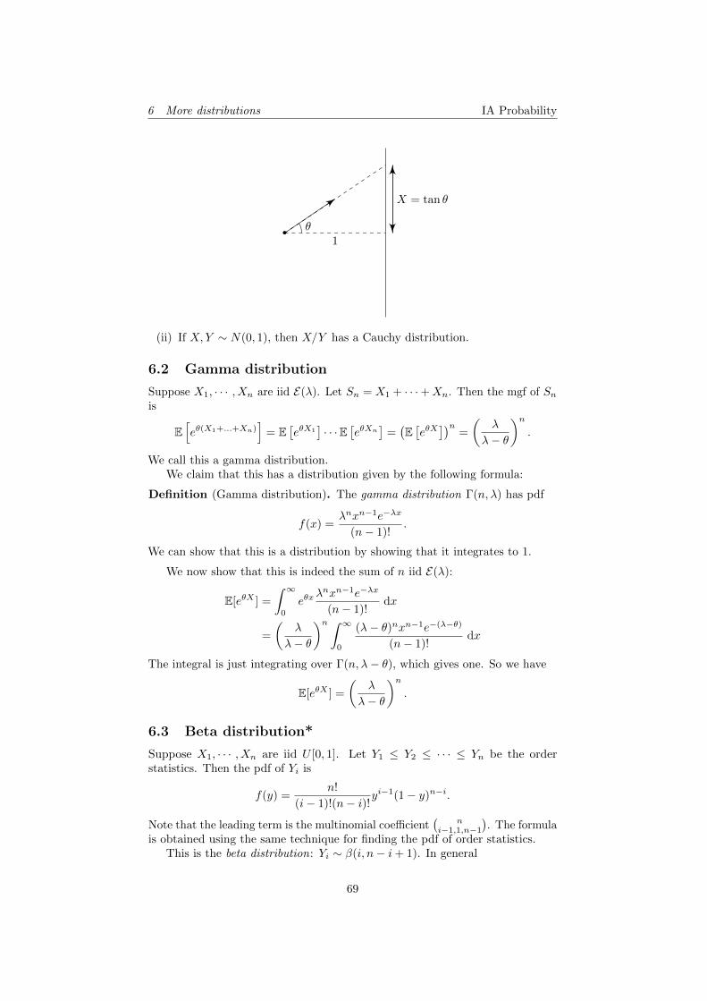
6 More distributions IA Probability
1θ
X = tan θ
(ii) If X,Y ∼ N(0, 1), then X/Y has a Cauchy distribution.
6.2 Gamma distribution
Suppose X1, · · · , Xn are iid E(λ). Let Sn = X1 + · · ·+Xn. Then the mgf of Snis
E[eθ(X1+...+Xn)
]= E
[eθX1
]· · ·E
[eθXn
]=(E[eθX
])n=
(λ
λ− θ
)n.
We call this a gamma distribution.We claim that this has a distribution given by the following formula:
Definition (Gamma distribution). The gamma distribution Γ(n, λ) has pdf
f(x) =λnxn−1e−λx
(n− 1)!.
We can show that this is a distribution by showing that it integrates to 1.
We now show that this is indeed the sum of n iid E(λ):
E[eθX ] =
∫ ∞0
eθxλnxn−1e−λx
(n− 1)!dx
=
(λ
λ− θ
)n ∫ ∞0
(λ− θ)nxn−1e−(λ−θ)
(n− 1)!dx
The integral is just integrating over Γ(n, λ− θ), which gives one. So we have
E[eθX ] =
(λ
λ− θ
)n.
6.3 Beta distribution*
Suppose X1, · · · , Xn are iid U [0, 1]. Let Y1 ≤ Y2 ≤ · · · ≤ Yn be the orderstatistics. Then the pdf of Yi is
f(y) =n!
(i− 1)!(n− i)!yi−1(1− y)n−i.
Note that the leading term is the multinomial coefficient(
ni−1,1,n−1
). The formula
is obtained using the same technique for finding the pdf of order statistics.This is the beta distribution: Yi ∼ β(i, n− i+ 1). In general
69
6 More distributions IA Probability
Definition (Beta distribution). The beta distribution β(a, b) has pdf
f(x; a, b) =Γ(a+ b)
Γ(a)Γ(b)xa−1(1− x)b−1
for 0 ≤ x ≤ 1.This has mean a/(a+ b).
Its moment generating function is
m(θ) = 1 +
∞∑k=1
(k−1∏r=0
a+ r
a+ b+ r
)θk
k!,
which is horrendous!
6.4 More on the normal distribution
Proposition. The moment generating function of N(µ, σ2) is
E[eθX ] = exp
(θµ+
1
2θ2σ2
).
Proof.
E[eθX ] =
∫ ∞−∞
eθx1√2πσ
e−12σ
2(x−µ)2 dx.
Substitute z = x−µσ . Then
E[eθX ] =
∫ ∞−∞
1√2πeθ(µ+σz)e−
12 z
2
dz
= eθµ+ 12 θ
2σ2
∫ ∞−∞
1√2πe−
12 (z−θσ)2︸ ︷︷ ︸
pdf of N(σθ,1)
dz
= eθµ+ 12 θ
2σ2
.
Theorem. Suppose X,Y are independent random variables with X ∼ N(µ1, σ21),
and Y ∼ (µ2, σ22). Then
(i) X + Y ∼ N(µ1 + µ2, σ21 + σ2
2).
(ii) aX ∼ N(aµ1, a2σ2
1).
Proof.
(i)
E[eθ(X+Y )] = E[eθX ] · E[eθY ]
= eµ1θ+12σ
21θ
2
· eµ2θ+12σ
22θ
= e(µ1+µ2)θ+ 12 (σ2
1+σ22)θ2
which is the mgf of N(µ1 + µ2, σ21 + σ2
2).
70
6 More distributions IA Probability
(ii)
E[eθ(aX)] = E[e(θa)X ]
= eµ(aθ)+ 12σ
2(aθ)2
= e(aµ)θ+ 12 (a2σ2)θ2
Finally, suppose X ∼ N(0, 1). Write φ(x) = 1√2πe−x
2/2 for its pdf. It would
be very difficult to find a closed form for its cumulative distribution function,but we can find an upper bound for it:
P(X ≥ x) =
∫ ∞x
φ(t) dt
≤∫ ∞x
(1 +
1
t2
)φ(t) dt
=1
xφ(x)
To see the last step works, simply differentiate the result and see that you get(1 + 1
x2
)φ(x). So
P(X ≥ x) ≤ 1
x
1√2πe−
12x
2
.
Then
logP(X ≥ x) ∼ −1
2x2.
6.5 Multivariate normal
Let X1, · · · , Xn be iid N(0, 1). Then their joint density is
g(x1, · · · , xn) =
n∏i=1
φ(xi)
=n∏1
1√2πe−
12x
2i
=1
(2π)n/2e−
12
∑n1 x
2i
=1
(2π)n/2e−
12x
Tx,
where x = (x1, · · · , xn)T .This result works if X1, · · · , Xn are iid N(0, 1). Suppose we are interested in
Z = µ +AX,
where A is an invertible n× n matrix. We can think of this as n measurementsZ that are affected by underlying standard-normal factors X. Then
X = A−1(Z− µ)
and
|J | = |det(A−1)| = 1
detA
71
6 More distributions IA Probability
So
f(z1, · · · , zn) =1
(2π)n/21
detAexp
[−1
2
((A−1(z− µ))T (A−1(z− µ))
)]=
1
(2π)n/2 detAexp
[−1
2(z− µ)TΣ−1(z− µ)
]=
1
(2π)n/2√
det Σexp
[−1
2(z− µ)TΣ−1(z− µ)
].
where Σ = AAT and Σ−1 = (A−1)TA−1. We say
Z =
Z1
...Zn
∼MVN(µ,Σ) or N(µ,Σ).
This is the multivariate normal.What is this matrix Σ? Recall that cov(Zi, Zj) = E[(Zi − µi)(Zj − µj)]. It
turns out this covariance is the i, jth entry of Σ, since
E[(Z− µ)(Z− µ)T ] = E[AX(AX)T ]
= E(AXXTAT ) = AE[XXT ]AT
= AIAT
= AAT
= Σ
So we also call Σ the covariance matrix.In the special case where n = 1, this is a normal distribution and Σ = σ2.Now suppose Z1, · · · , Zn have covariances 0. Then Σ = diag(σ2
1 , · · · , σ2n).
Then
f(z1, · · · , zn) =
n∏1
1√2πσi
e− 1
2σ2i
(zi−µi)2.
So Z1, · · · , Zn are independent, with Zi ∼ N(µi, σ2i ).
Here we proved that if cov = 0, then the variables are independent. However,this is only true when Zi are multivariate normal. It is generally not true forarbitrary distributions.
For these random variables that involve vectors, we will need to modify ourdefinition of moment generating functions. We define it to be
m(θ) = E[eθTX] = E[eθ1X1+···+θnXn ].
Bivariate normal
This is the special case of the multivariate normal when n = 2. Since therearen’t too many terms, we can actually write them out.
The bivariate normal has
Σ =
(σ2
1 ρσ1σ2
ρσ1σ2 σ22
).
72
6 More distributions IA Probability
Then
corr(X1, X2) =cov(X1, X2)√
var(X1) var(X2)=ρσ1σ2
σ1σ2= ρ.
And
Σ−1 =1
1− ρ2
(σ−2
1 −ρσ−11 σ−1
2
−ρσ−11 σ−1
2 σ−22
)The joint pdf of the bivariate normal with zero mean is
f(x1, x2) =1
2πσ1σ2
√1− ρ2
exp
(− 1
2(1− ρ2)
(x2
1
σ21
− 2ρx1x2
σ1σ2+x2
2
σ22
))If the mean is non-zero, replace xi with xi − µi.
The joint mgf of the bivariate normal is
m(θ1, θ2) = eθ1µ1+θ2µ2+ 12 (θ21σ
21+2θ1θ2ρσ1σ2+θ22σ
22).
Nice and elegant.
73
7 Central limit theorem IA Probability
7 Central limit theorem
Suppose X1, · · · , Xn are iid random variables with mean µ and variance σ2. LetSn = X1 + · · ·+Xn. Then we have previously shown that
var(Sn/√n) = var
(Sn − nµ√
n
)= σ2.
Theorem (Central limit theorem). Let X1, X2, · · · be iid random variables withE[Xi] = µ, var(Xi) = σ2 <∞. Define
Sn = X1 + · · ·+Xn.
Then for all finite intervals (a, b),
limn→∞
P(a ≤ Sn − nµ
σ√n≤ b)
=
∫ b
a
1√2πe−
12 t
2
dt.
Note that the final term is the pdf of a standard normal. We say
Sn − nµσ√n→D N(0, 1).
To show this, we will use the continuity theorem without proof:
Theorem (Continuity theorem). If the random variables X1, X2, · · · have mgf’sm1(θ),m2(θ), · · · and mn(θ) → m(θ) as n → ∞ for all θ, then Xn →D therandom variable with mgf m(θ).
We now provide a sketch-proof of the central limit theorem:
Proof. wlog, assume µ = 0, σ2 = 1 (otherwise replace Xi with Xi−µσ ).
Then
mXi(θ) = E[eθXi ] = 1 + θE[Xi] +θ2
2!E[X2
i ] + · · ·
= 1 +1
2θ2 +
1
3!θ3E[X3
i ] + · · ·
Now consider Sn/√n. Then
E[eθSn/√n] = E[eθ(X1+...+Xn)/
√n]
= E[eθX1/√n] · · ·E[eθXn/
√n]
=(E[eθX1/
√n])n
=
(1 +
1
2θ2 1
n+
1
3!θ3E[X3]
1
n3/2+ · · ·
)n→ e
12 θ
2
as n→∞ since (1 + a/n)n → ea. And this is the mgf of the standard normal.So the result follows from the continuity theorem.
74
7 Central limit theorem IA Probability
Note that this is not a very formal proof, since we have to require E[X3] tobe finite. Also, sometimes the moment generating function is not defined. Butthis will work for many “nice” distributions we will ever meet.
The proper proof uses the characteristic function
χX(θ) = E[eiθX ].
An important application is to use the normal distribution to approximate alarge binomial.
Let Xi ∼ B(1, p). Then Sn ∼ B(n, p). So E[Sn] = np and var(Sn) = p(1−p).So
Sn − np√np(1− p)
→D N(0, 1).
Example. Suppose two planes fly a route. Each of n passengers chooses a planeat random. The number of people choosing plane 1 is S ∼ B(n, 1
2 ). Supposeeach has s seats. What is
F (s) = P(S > s),
i.e. the probability that plane 1 is over-booked? We have
F (s) = P(S > s) = P
S − n/2√n · 1
2 ·12
>s− n/2√n/2
.
SinceS − np√n/2
∼ N(0, 1),
we have
F (s) ≈ 1− Φ
(s− n/2√n/2
).
For example, if n = 1000 and s = 537, then Sn−n/2√n/2
≈ 2.34, Φ(2.34) ≈ 0.99,
and F (s) ≈ 0.01. So with only 74 seats as buffer between the two planes, theprobability of overbooking is just 1/100.
Example. An unknown proportion p of the electorate will vote Labour. It isdesired to find p without an error not exceeding 0.005. How large should thesample be?
We estimate by
p′ =Snn,
where Xi ∼ B(1, p). Then
P(|p′ − p| ≤ 0.005) = P(|Sn − np| ≤ 0.005n)
= P
|Sn − np|√np(1− p)︸ ︷︷ ︸≈N(0,1)
≤ 0.005n√np(1− p)
75
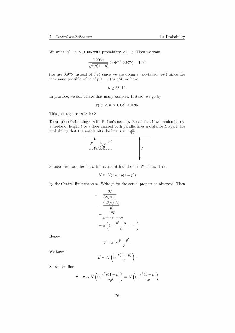
7 Central limit theorem IA Probability
We want |p′ − p| ≤ 0.005 with probability ≥ 0.95. Then we want
0.005n√np(1− p)
≥ Φ−1(0.975) = 1.96.
(we use 0.975 instead of 0.95 since we are doing a two-tailed test) Since themaximum possible value of p(1− p) is 1/4, we have
n ≥ 38416.
In practice, we don’t have that many samples. Instead, we go by
P(|p′ < p| ≤ 0.03) ≥ 0.95.
This just requires n ≥ 1068.
Example (Estimating π with Buffon’s needle). Recall that if we randomly tossa needle of length ` to a floor marked with parallel lines a distance L apart, theprobability that the needle hits the line is p = 2`
πL .
`Xθ L
Suppose we toss the pin n times, and it hits the line N times. Then
N ≈ N(np, np(1− p))
by the Central limit theorem. Write p′ for the actual proportion observed. Then
π =2`
(N/n)L
=π2`/(πL)
p′
=πp
p+ (p′ − p)
= π
(1− p′ − p
p+ · · ·
)Hence
π − π ≈ p− p′
p.
We know
p′ ∼ N(p,p(1− p)
n
).
So we can find
π − π ∼ N(
0,π2p(1− p)
np2
)= N
(0,π2(1− p)
np
)
76
7 Central limit theorem IA Probability
We want a small variance, and that occurs when p is the largest. Since p = 2`/πL,this is maximized with ` = L. In this case,
p =2
π,
and
π − π ≈ N(
0,(π − 2)π2
2n
).
If we want to estimate π to 3 decimal places, then we need
P(|π − π| ≤ 0.001) ≥ 0.95.
This is true if and only if
0.001
√2n
(π − 2)(π2)≥ Φ−1(0.975) = 1.96
So n ≥ 2.16× 10⁷. So we can obtain π to 3 decimal places just by throwing astick 20 million times! Isn’t that exciting?
77
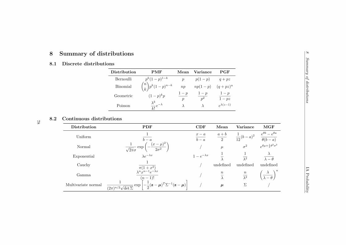
8S
um
mary
of
distribu
tion
sIA
Prob
ability
8 Summary of distributions
8.1 Discrete distributions
Distribution PMF Mean Variance PGF
Bernoulli pk(1− p)1−k p p(1− p) q + pz
Binomial
(n
k
)pk(1− p)n−k np np(1− p) (q + pz)n
Geometric (1− p)kp 1− pp
1− pp2
1− p1− pz
Poissonλk
k!e−λ λ λ eλ(z−1)
8.2 Continuous distributions
Distribution PDF CDF Mean Variance MGF
Uniform1
b− ax− ab− a
a+ b
2
1
12(b− a)2 eθb − eθa
θ(b− a)
Normal1√2πσ
exp
(− (x− µ)2
2σ2
)/ µ σ2 eθµ+ 1
2 θ2σ2
Exponential λe−λx 1− e−λx 1
λ
1
λ2
λ
λ− θCauchy
1
π(1 + x2)/ undefined undefined undefined
Gammaλnxn−1e−λx
(n− 1)!/
n
λ
n
λ2
(λ
λ− θ
)nMultivariate normal
1
(2π)n/2√
det Σexp
[−1
2(z− µ)TΣ−1(z− µ)
]/ µ Σ /
78