Embed Size (px)
Citation preview
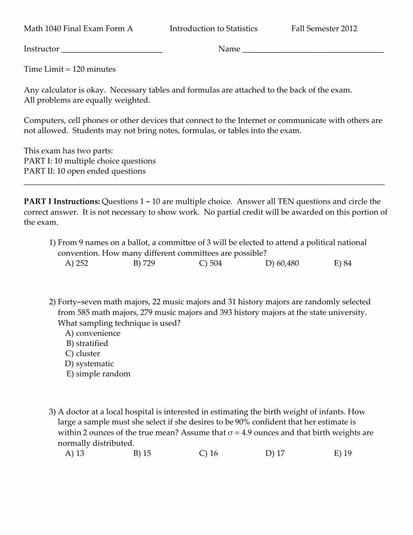
Math 1040 Final Exam Form A Introduction to Statistics Fall Semester 2012
Instructor _________________________ Name ___________________________________
Time Limit = 120 minutes
Any calculator is okay. Necessary tables and formulas are attached to the back of the exam.All problems are equally weighted.
Computers, cell phones or other devices that connect to the Internet or communicate with others arenot allowed. Students may not bring notes, formulas, or tables into the exam.
This exam has two parts:PART I: 10 multiple choice questionsPART II: 10 open ended questions_________________________________________________________________________________________
PART I Instructions: Questions 1 - 10 are multiple choice. Answer all TEN questions and circle the
correct answer. It is not necessary to show work. No partial credit will be awarded on this portion ofthe exam.
1) From 9 names on a ballot, a committee of 3 will be elected to attend a political national
convention. How many different committees are possible?A) 252 B) 729 C) 504 D) 60,480 E) 84
2) Forty-seven math majors, 22 music majors and 31 history majors are randomly selected
from 585 math majors, 279 music majors and 393 history majors at the state university.
What sampling technique is used?A) convenienceB) stratifiedC) clusterD) systematicE) simple random
3) A doctor at a local hospital is interested in estimating the birth weight of infants. Howlarge a sample must she select if she desires to be 90% confident that her estimate is
within 2 ounces of the true mean? Assume that σ = 4.9 ounces and that birth weights are
normally distributed.A) 13 B) 15 C) 16 D) 17 E) 19

4) According to the law of large numbers, as more observations are added to the sample, thedifference between the sample mean and the population mean
A) Remains about the sameB) Tends to become smallerC) Is inversely affected by the data addedD) Tends to become larger
5) The length of time it takes college students to find a parking spot in the library parkinglot follows a normal distribution with a mean of 6.5 minutes and a standard deviation of 1
minute. Find the probability that a randomly selected college student will take between5.0 and 7.5 minutes to find a parking spot in the library lot.
A) 0.4938 B) 0.0919 C) 0.7745 D) 0.2255
6) A researcher wishes to construct a confidence interval for a population mean μ. If thesample size is 19, what conditions must be satisfied to compute the confidence interval?
A) The population standard deviation σ must be known.
B) It must be true that np^(1-p
^) ≥ 10 and n ≤ 0.05N.
C) The data must come from a population that is approximately normal with nooutliers.
D) The confidence level cannot be greater than 90%.
7) Investing is a game of chance. Suppose there is a 36% chance that a risky stock investment
will end up in a total loss of your investment. Because the rewards are so high, you decideto invest in five independent risky stocks. Find the probability that at least one of your
five investments becomes a total loss.
A) 0.8926 B) 0.0604 C) 0.006 D) 0.302
8) If we do not reject the null hypothesis when the null hypothesis is in error, then we havemade a
A) Type I error B) Correct decisionC) Type II error D) Type β error

9) What effect would increasing the sample size have on a confidence interval?A) No change B) Change the confidence levelC) Increase the width of the interval D) Decrease the width of the interval
10) A seed company has a test plot in which it is testing the germination of a hybrid seed.They plant 50 rows of 40 seeds per row. After a two-week period, the researchers count
how many seeds per row have sprouted. They noted that the least number of seeds togerminate was 33 and some rows had all 40 germinate. The germination data is given
below in the table. The random variable X represents the number of seeds in a row that
germinated and P(x) represents the probability of selecting a row with that number ofseeds germinating. Determine the expected number of seeds per row that germinated.
x 33 34 35 36 37 38 39 40
P(x) 0.02 0.06 0.10 0.20 0.24 0.26 0.10 0.02
A) 1.51 B) 4.61 C) 36.50 D) 36.86 E) 37.00
_________________________________________________________________________________________
PART II Instructions: Questions 11 - 20 are open response. Answer all TEN questions carefully and
completely, for full credit you must show all appropriate work and clearly indicate your answers._________________________________________________________________________________________
11) The owner of a computer repair shop has determined that their daily revenue has mean$7200 and standard deviation $1200. The daily revenue totals for the next 30 days will bemonitored. What is the probability that the mean daily revenue for the next 30 days willexceed $7500? Round your answer to 4 decimal places.

12) The costs in dollars of a random sample of 20 college textbooks are given in thestem-and-leaf plot below.
Stem Leaves
2 7 8
3 6
4 0 2
5 3
6 7
7 1 6 9 9
8 2 4 4
9 0 3 5 7
10 5 7
Legend: 2 7 represents $27
i) Find the five number summary for this data set. Include the name or correct symbolfor each of the numbers as well as its value.
ii) Draw a boxplot of this data set.
iii) Use complete sentences to briefly describe the shape of the distribution for this data.
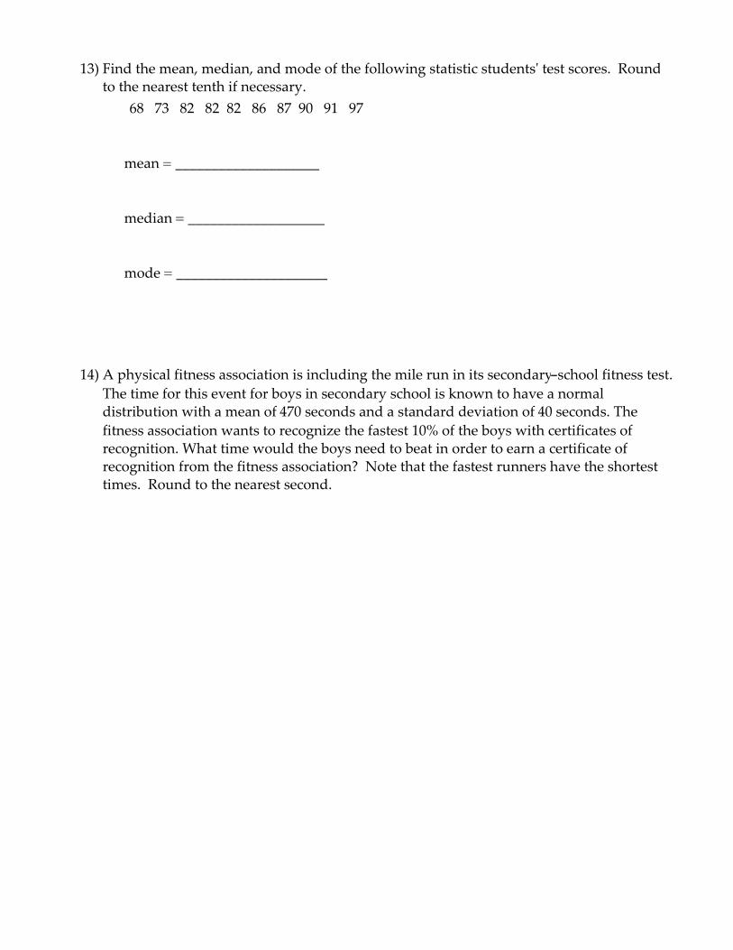
13) Find the mean, median, and mode of the following statistic students' test scores. Roundto the nearest tenth if necessary.
68 73 82 82 82 86 87 90 91 97
mean = ____________________
median = ___________________
mode = _____________________
14) A physical fitness association is including the mile run in its secondary-school fitness test.
The time for this event for boys in secondary school is known to have a normaldistribution with a mean of 470 seconds and a standard deviation of 40 seconds. The
fitness association wants to recognize the fastest 10% of the boys with certificates ofrecognition. What time would the boys need to beat in order to earn a certificate ofrecognition from the fitness association? Note that the fastest runners have the shortesttimes. Round to the nearest second.

15) The data below are the final exam scores of 10 randomly selected history students and thenumber of hours they slept the night before the exam.
Hours, x
Scores, y
3
65
5
80
2
60
8
88
2
66
4
78
4
85
5
90
6
90
3
71
The scatterplot for this data:
x1 2 3 4 5 6 7 8 9 10
y
90
85
80
75
70
65
60
Hours of Sleep
Ex
am S
core
s
x1 2 3 4 5 6 7 8 9 10
y
90
85
80
75
70
65
60
Hours of Sleep
Ex
am S
core
s
i) Based on the scatterplot, is it reasonable to suggest that there is a linear relationshipbetween hours of sleep and exam scores? Yes or No (circle one)
ii) Find the correlation coefficient for the given data. Round to 4 decimal places.
iii) Determine if there is a significant linear correlation. Report the critical value and stateyour conclusion.
iv) Find the equation of the least-squares regression line for this data. Round values to 2
decimal places.
v) Use the regression equation to predict the exam score of a student who slept for 7hours the night before the exam. Is the predicted exam score a good estimate? Brieflyexplain your answer.

16) A random sample of 20 college students is selected. Each student is asked how muchtime he or she spent on the Internet during the previous week. The following times (inhours) are recorded:
8 12 3 15 16 5 16 5 6 10
3 12 13 4 4 11 9 17 14 12
i) Create a frequency and relative frequency table for this data. Use 3 as the lower classlimit of the first class, and use a class width of 4.
ClassTally
(optional) FrequencyRelative
Frequency
ii) Create a relative frequency histogram for the data. Be sure to label your axes.
x
y
x
y

17) When 440 junior college students were surveyed, 200 said they have a passport. Construct
a 95% confidence interval for the proportion of junior college students that have apassport. Round to the nearest thousandth.
18) The National Association of Realtors estimates that 23% of all homes purchased in 2004were considered investment properties. If a sample of 800 homes sold in 2004 is obtainedwhat is the probability that at most 200 homes are going to be used as investmentproperty? Round your answer to 4 decimal places.

19) In 2010, 36% of adults in a certain country were morbidly obese. A health practitionersuspects that the percent has changed since then. She obtains a random sample of 1042adults and finds that 393 are morbidly obese. Is this sufficient evidence to support thepractitioner's suspicion that the percent of morbidly obese adults has changed at theα = 0.10 level of significance?
Are you using the Classical or P-Value approach? (circle one)
Null Hypothesis:
Alternative Hypothesis:
Test Statistic:
Critical Value(s) or P-Value (circle which of these you are using):
Conclusion about the Null Hypothesis:
Do the data support the health practitioner's suspicion? Answer with complete sentences.

20) A shipping firm suspects that the mean life of a certain brand of tire used by its trucks isless than 40,000 miles. To check the hypothesis, the firm randomly selects and tests 18 of
these tires and finds that they have a mean lifetime of 39,300 miles with a standard
deviation of 1200 miles. At α = 0.05, test the shipping firm's hypothesis. Assume that the
life of the tires is normally distributed with no outliers. Show a complete solutionincluding all your steps.

Tables and Formulas for Sullivan, Statistics: Informed Decisions Using Data ©2010 Pearson Education, Inc
Chapter 2 Organizing and Summarizing Data
• Class midpoint: The sum of consecutive lower class limitsdivided by 2.
• Relative frequency =frequency
sum of all frequencies
Chapter 3 Numerically Summarizing Data
• Population Mean:
• Sample Mean:
•
• Population Variance:
• Sample Variance:
• Population Standard Deviation:
• Sample Standard Deviation:
• Empirical Rule: If the shape of the distribution is bell-shaped, then
• Approximately 68% of the data lie within 1 standarddeviation of the mean
• Approximately 95% of the data lie within 2 standarddeviations of the mean
• Approximately 99.7% of the data lie within 3 stan-dard deviations of the mean
• Population Mean from Grouped Data:
• Sample Mean from Grouped Data: x =gxifigfi
m =gxifigfi
s = 2s2s = 2s2
s2 =g1xi - x22n - 1
=
gx2i -1gxi22n
n - 1
s2 =g1xi - m22N
=
gx2i -1 gxi22N
N
Range = Largest Data Value - Smallest Data Value
x =gxin
m =gxiN
• Weighted Mean:
• Population Variance from Grouped Data:
• Sample Variance from Grouped Data:
• Population z-score:
• Sample z-score:
• Interquartile Range:
• Lower and Upper Fences:
• Five-Number Summary
Minimum, Q1 , M, Q3 , Maximum
Lower fence = Q1 - 1.51IQR2Upper fence = Q3 + 1.51IQR2
IQR = Q3 - Q1
z =x - x
s
z =x - m
s
s2 =g1xi - m22fiAgfi B - 1
=
gx2ifi -
1gxifi22gfi
gfi - 1
s2 =g1xi - m22fi
gfi=
gx2ifi -
1gxifi22gfi
gfi
xw =gwixigwi
CHAPTER 4 Describing the Relation between Two Variables
• observed
• for the least-squares regression model
• The coefficient of determination, measures theproportion of total variation in the response variablethat is explained by the least-squares regression line.
R2,
yN = b1x + b0
R2 = r2
y - predicted y = y - yNResidual =
• Correlation Coefficient:
• The equation of the least-squares regression line is
where is the predicted value,
is the slope, and is the intercept.b0 = y - b1x
b1 = r #sy
sxyNyN = b1x + b0,
r =
a axi - xsx b ayi - ysyb
n - 1
CHAPTER 5 Probability
• Empirical Probability
• Classical Probability
P1E2 =number of ways that E can occur
number of possible outcomes=N1E2N1S2
P1E2 Lfrequency of E
number of trials of experiment
• Addition Rule for Disjoint Events
• Addition Rule for n Disjoint Events
• General Addition Rule
P1E or F2 = P1E2 + P1F2 - P1E and F2
P1E or F or G or Á 2 = P1E2 + P1F2 + P1G2 + Á
P1E or F2 = P1E2 + P1F2

Tables and Formulas for Sullivan, Statistics: Informed Decisions Using Data ©2010 Pearson Education, Inc
CHAPTER 6 Discrete Probability Distributions
• Mean and Standard Deviation of a Binomial RandomVariable
• Poisson Probability Distribution Function
• Mean and Standard Deviation of a Poisson Random Variable
mX = lt sX = 2lt
P1x2 =1lt2xx!e-lt x = 0, 1, 2, Á
sX = 4np11 - p2mX = np
• Mean (Expected Value) of a Discrete Random Variable
• Variance of a Discrete Random Variable
• Binomial Probability Distribution Function
P1x2 = nCxpx11 - p2n-x
s2X = g1x - m22 # P1x2 = gx2P1x2 - m2
X
mX = gx # P1x2
CHAPTER 7 The Normal Distribution
• Standardizing a Normal Random Variable
z =x - m
s
• Finding the Score: x = m + zs
CHAPTER 8 Sampling Distributions
• Mean and Standard Deviation of the Sampling Distribu-tion of
• Sample Proportion: pN =x
n
mx = m and sx =s
2nx
• Mean and Standard Deviation of the SamplingDistribution of
mpN = p and spN = Cp11 - p2n
pN
CHAPTER 9 Estimating the Value of a Parameter Using Confidence Intervals
Confidence Intervals
• A confidence interval about with
known is .
• A confidence interval about with
unknown is . Note: is computed using
degrees of freedom.
• A confidence interval about p is
.
• A confidence interval about is
.1n - 12s2xa/2
26 s2 6
1n - 12s2x1-a/2
2
s211 - a2 # 100%
pn ; za/2# CpN11 - pn2n
11 - a2 # 100%
n - 1
ta/2x ; ta/2# s1n
sm11 - a2 # 100%
x ; za/2# s1n
sm11 - a2 # 100%
Sample Size
• To estimate the population mean with a margin of error E
at a level of confidence:
rounded up to the next integer.
• To estimate the population proportion with a marginof error E at a level of confidence:
rounded up to the next integer,
where is a prior estimate of the population proportion,
or rounded up to the next integer when
no prior estimate of p is available.
n = 0.25 a za/2
Eb2
pN
n = pN11 - pN2a za/2
Eb2
11 - a2 # 100%
n = a za/2# sEb211 - a2 # 100%
• Complement Rule
• Multiplication Rule for Independent Events
• Multiplication Rule for n Independent Events
• Conditional Probability Rule
• General Multiplication Rule
P1E and F2 = P1E2 # P1F ƒE2
P1F ƒE2 =P1E and F2P1E2 =
N1E and F2N1E2
P1E and F and GÁ 2 = P1E2 # P1F2 # P1G2 # Á
P1E and F2 = P1E2 # P1F2
P1Ec2 = 1 - P1E2• Factorial
• Permutation of n objects taken r at a time:
• Combination of n objects taken r at a time:
• Permutations with Repetition:
n!
n1! # n2! # Á # nk!
nCr =n!
r!1n - r2!
nPr =n!
1n - r2!n! = n # 1n - 12 # 1n - 22 # Á # 3 # 2 # 1

Tables and Formulas for Sullivan, Statistics: Informed Decisions Using Data ©2010 Pearson Education, Inc
CHAPTER 10 Testing Claims Regarding a Parameter
•
• x20 =1n - 12s2s0
2
z0 =pN - p0
Cp011 - p02
n
CHAPTER 11 Inferences on Two Samples
• Test Statistic for Matched-Pairs data
where is the mean and is the standard deviation ofthe differenced data.
• Confidence Interval for Matched-Pairs data:
Note: is found using degrees of freedom.
• Test Statistic Comparing Two Means (Independent Sampling):
• Confidence Interval for the Difference of Two Means(Independent Samples):
1x1 - x22 ; ta/2Cs1
2
n1
+s2
2
n2
t0 =1x1 - x22 - 1m1 - m22
Cs1
2
n1
+s2
2
n2
n - 1ta/2
d ; ta/2# sd1n
sdd
t0 =d - mdsdn1n
Note: is found using the smaller of or degrees of freedom.
• Test Statistic Comparing Two Population Proportions
where
• Confidence Interval for the Difference of Two Proportions
• Test Statistic for Comparing Two Population StandardDeviations
• Finding a Critical F for the Left Tail
F1-a,n1-1,n2-1 =1
Fa,n2-1,n1-1
F0 =s1
2
s22
1pN1 - pN22 ; za/2CpN111 - pN12n1
+pN211 - pN22n2
pN =x1 + x2
n1 + n2
.z0 =pN1 - pN2 - (p1 - p2)
4pN11 - pN2B1
n1
+1
n2
n2 - 1n1 - 1ta/2
Test Statistics
• single mean, known
• single mean, unknownst0 =
x - m0
sn1n
sz0 =
x - m0
sn1n
CHAPTER 12 Inference on Categorical Data
• Chi-Square Test Statistic
All and no more than 20% less than 5.Ei Ú 1
i = 1, 2, Á , k
x20 = a
1observed - expected22expected
= a1Oi - Ei22Ei
• Expected Counts (when testing for goodness of fit)
• Expected Frequencies (when testing for independence orhomogeneity of proportions)
Expected frequency =1row total21column total2
table total
Ei = mi = npi for i = 1, 2, Á , k
CHAPTER 13 Comparing Three or More Means
• Test Statistic for One-Way ANOVA
where
MSE =1n1 - 12s12 + 1n2 - 12s22 + Á + 1nk - 12sk2
n - k
MST =n11x1 - x22 + n21x2 - x22 + Á + nk1xk - x22
k - 1
F =Mean square due to treatment
Mean square due to error=
MST
MSE
• Test Statistic for Tukey’s Test after One-Way ANOVA
q =1x2 - x12 - 1m2 - m12
As2
2 # a 1
n1
+1
n2b
=x2 - x1
As2
2# a 1
n1
+1
n2
b

Tables and Formulas for Sullivan, Statistics: Informed Decisions Using Data ©2010 Pearson Education, Inc
Table I
Row
Number 01–05 06–10 11–15 16–20 21–25 26–30 31–35 36–40 41–45 46–50
01 89392 23212 74483 36590 25956 36544 68518 40805 09980 0046702 61458 17639 96252 95649 73727 33912 72896 66218 52341 9714103 11452 74197 81962 48443 90360 26480 73231 37740 26628 4469004 27575 04429 31308 02241 01698 19191 18948 78871 36030 23980
05 36829 59109 88976 46845 28329 47460 88944 08264 00843 8459206 81902 93458 42161 26099 09419 89073 82849 09160 61845 4090607 59761 55212 33360 68751 86737 79743 85262 31887 37879 1752508 46827 25906 64708 20307 78423 15910 86548 08763 47050 1851309 24040 66449 32353 83668 13874 86741 81312 54185 78824 0071810 98144 96372 50277 15571 82261 66628 31457 00377 63423 55141
11 14228 17930 30118 00438 49666 65189 62869 31304 17117 7148912 55366 51057 90065 14791 62426 02957 85518 28822 30588 3279813 96101 30646 35526 90389 73634 79304 96635 06626 94683 1669614 38152 55474 30153 26525 83647 31988 82182 98377 33802 8047115 85007 18416 24661 95581 45868 15662 28906 36392 07617 50248
16 85544 15890 80011 18160 33468 84106 40603 01315 74664 2055317 10446 20699 98370 17684 16932 80449 92654 02084 19985 5932118 67237 45509 17638 65115 29757 80705 82686 48565 72612 6176019 23026 89817 05403 82209 30573 47501 00135 33955 50250 7259220 67411 58542 18678 46491 13219 84084 27783 34508 55158 78742
Column Number
Random Numbers
Table II
Critical Values for Correlation Coefficient
n
3 0.997
4 0.950
5 0.878
6 0.811
7 0.754
8 0.707
9 0.666
n
10 0.632
11 0.602
12 0.576
13 0.553
14 0.532
15 0.514
16 0.497
n
17 0.482
18 0.468
19 0.456
20 0.444
21 0.433
22 0.423
23 0.413
n
24 0.404
25 0.396
26 0.388
27 0.381
28 0.374
29 0.367
30 0.361

Tables and Formulas for Sullivan, Statistics: Informed Decisions Using Data ©2010 Pearson Education, Inc
23.4 0.0003 0.0003 0.0003 0.0003 0.0003 0.0003 0.0003 0.0003 0.0003 0.0002
23.3 0.0005 0.0005 0.0005 0.0004 0.0004 0.0004 0.0004 0.0004 0.0004 0.0003
23.2 0.0007 0.0007 0.0006 0.0006 0.0006 0.0006 0.0006 0.0005 0.0005 0.0005
23.1 0.0010 0.0009 0.0009 0.0009 0.0008 0.0008 0.0008 0.0008 0.0007 0.0007
23.0 0.0013 0.0013 0.0013 0.0012 0.0012 0.0011 0.0011 0.0011 0.0010 0.0010
22.9 0.0019 0.0018 0.0018 0.0017 0.0016 0.0016 0.0015 0.0015 0.0014 0.0014
22.8 0.0026 0.0025 0.0024 0.0023 0.0023 0.0022 0.0021 0.0021 0.0020 0.0019
22.7 0.0035 0.0034 0.0033 0.0032 0.0031 0.0030 0.0029 0.0028 0.0027 0.0026
22.6 0.0047 0.0045 0.0044 0.0043 0.0041 0.0040 0.0039 0.0038 0.0037 0.0036
22.5 0.0062 0.0060 0.0059 0.0057 0.0055 0.0054 0.0052 0.0051 0.0049 0.0048
22.4 0.0082 0.0080 0.0078 0.0075 0.0073 0.0071 0.0069 0.0068 0.0066 0.0064
22.3 0.0107 0.0104 0.0102 0.0099 0.0096 0.0094 0.0091 0.0089 0.0087 0.0084
22.2 0.0139 0.0136 0.0132 0.0129 0.0125 0.0122 0.0119 0.0116 0.0113 0.0110
22.1 0.0179 0.0174 0.0170 0.0166 0.0162 0.0158 0.0154 0.0150 0.0146 0.0143
22.0 0.0228 0.0222 0.0217 0.0212 0.0207 0.0202 0.0197 0.0192 0.0188 0.0183
21.9 0.0287 0.0281 0.0274 0.0268 0.0262 0.0256 0.0250 0.0244 0.0239 0.0233
21.8 0.0359 0.0351 0.0344 0.0336 0.0329 0.0322 0.0314 0.0307 0.0301 0.0294
21.7 0.0446 0.0436 0.0427 0.0418 0.0409 0.0401 0.0392 0.0384 0.0375 0.0367
21.6 0.0548 0.0537 0.0526 0.0516 0.0505 0.0495 0.0485 0.0475 0.0465 0.0455
21.5 0.0668 0.0655 0.0643 0.0630 0.0618 0.0606 0.0594 0.0582 0.0571 0.0559
21.4 0.0808 0.0793 0.0778 0.0764 0.0749 0.0735 0.0721 0.0708 0.0694 0.0681
21.3 0.0968 0.0951 0.0934 0.0918 0.0901 0.0885 0.0869 0.0853 0.0838 0.0823
21.2 0.1151 0.1131 0.1112 0.1093 0.1075 0.1056 0.1038 0.1020 0.1003 0.0985
21.1 0.1357 0.1335 0.1314 0.1292 0.1271 0.1251 0.1230 0.1210 0.1190 0.1170
21.0 0.1587 0.1562 0.1539 0.1515 0.1492 0.1469 0.1446 0.1423 0.1401 0.1379
20.9 0.1841 0.1814 0.1788 0.1762 0.1736 0.1711 0.1685 0.1660 0.1635 0.1611
20.8 0.2119 0.2090 0.2061 0.2033 0.2005 0.1977 0.1949 0.1922 0.1894 0.1867
20.7 0.2420 0.2389 0.2358 0.2327 0.2296 0.2266 0.2236 0.2206 0.2177 0.2148
20.6 0.2743 0.2709 0.2676 0.2643 0.2611 0.2578 0.2546 0.2514 0.2483 0.2451
20.5 0.3085 0.3050 0.3015 0.2981 0.2946 0.2912 0.2877 0.2843 0.2810 0.2776
20.4 0.3446 0.3409 0.3372 0.3336 0.3300 0.3264 0.3228 0.3192 0.3156 0.3121
20.3 0.3821 0.3783 0.3745 0.3707 0.3669 0.3632 0.3594 0.3557 0.3520 0.3483
20.2 0.4207 0.4168 0.4129 0.4090 0.4052 0.4013 0.3974 0.3936 0.3897 0.3859
20.1 0.4602 0.4562 0.4522 0.4483 0.4443 0.4404 0.4364 0.4325 0.4286 0.4247
20.0 0.5000 0.4960 0.4920 0.4880 0.4840 0.4801 0.4761 0.4721 0.4681 0.4641
Standard Normal Distribution
Table V
z .00 .01 .02 .03 .04 .05 .06 .07 .08 .09Area
z
0.0 0.5000 0.5040 0.5080 0.5120 0.5160 0.5199 0.5239 0.5279 0.5319 0.5359
0.1 0.5398 0.5438 0.5478 0.5517 0.5557 0.5596 0.5636 0.5675 0.5714 0.5753
0.2 0.5793 0.5832 0.5871 0.5910 0.5948 0.5987 0.6026 0.6064 0.6103 0.6141
0.3 0.6179 0.6217 0.6255 0.6293 0.6331 0.6368 0.6406 0.6443 0.6480 0.6517
0.4 0.6554 0.6591 0.6628 0.6664 0.6700 0.6736 0.6772 0.6808 0.6844 0.6879
0.5 0.6915 0.6950 0.6985 0.7019 0.7054 0.7088 0.7123 0.7157 0.7190 0.7224
0.6 0.7257 0.7291 0.7324 0.7357 0.7389 0.7422 0.7454 0.7486 0.7517 0.7549
0.7 0.7580 0.7611 0.7642 0.7673 0.7704 0.7734 0.7764 0.7794 0.7823 0.7852
0.8 0.7881 0.7910 0.7939 0.7967 0.7995 0.8023 0.8051 0.8078 0.8106 0.8133
0.9 0.8159 0.8186 0.8212 0.8238 0.8264 0.8289 0.8315 0.8340 0.8365 0.8389
1.0 0.8413 0.8438 0.8461 0.8485 0.8508 0.8531 0.8554 0.8577 0.8599 0.8621
1.1 0.8643 0.8665 0.8686 0.8708 0.8729 0.8749 0.8770 0.8790 0.8810 0.8830
1.2 0.8849 0.8869 0.8888 0.8907 0.8925 0.8944 0.8962 0.8980 0.8997 0.9015
1.3 0.9032 0.9049 0.9066 0.9082 0.9099 0.9115 0.9131 0.9147 0.9162 0.9177
1.4 0.9192 0.9207 0.9222 0.9236 0.9251 0.9265 0.9279 0.9292 0.9306 0.9319
1.5 0.9332 0.9345 0.9357 0.9370 0.9382 0.9394 0.9406 0.9418 0.9429 0.9441
1.6 0.9452 0.9463 0.9474 0.9484 0.9495 0.9505 0.9515 0.9525 0.9535 0.9545
1.7 0.9554 0.9564 0.9573 0.9582 0.9591 0.9599 0.9608 0.9616 0.9625 0.9633
1.8 0.9641 0.9649 0.9656 0.9664 0.9671 0.9678 0.9686 0.9693 0.9699 0.9706
1.9 0.9713 0.9719 0.9726 0.9732 0.9738 0.9744 0.9750 0.9756 0.9761 0.9767
2.0 0.9772 0.9778 0.9783 0.9788 0.9793 0.9798 0.9803 0.9808 0.9812 0.9817
2.1 0.9821 0.9826 0.9830 0.9834 0.9838 0.9842 0.9846 0.9850 0.9854 0.9857
2.2 0.9861 0.9864 0.9868 0.9871 0.9875 0.9878 0.9881 0.9884 0.9887 0.9890
2.3 0.9893 0.9896 0.9898 0.9901 0.9904 0.9906 0.9909 0.9911 0.9913 0.9916
2.4 0.9918 0.9920 0.9922 0.9925 0.9927 0.9929 0.9931 0.9932 0.9934 0.9936
2.5 0.9938 0.9940 0.9941 0.9943 0.9945 0.9946 0.9948 0.9949 0.9951 0.9952
2.6 0.9953 0.9955 0.9956 0.9957 0.9959 0.9960 0.9961 0.9962 0.9963 0.9964
2.7 0.9965 0.9966 0.9967 0.9968 0.9969 0.9970 0.9971 0.9972 0.9973 0.9974
2.8 0.9974 0.9975 0.9976 0.9977 0.9977 0.9978 0.9979 0.9979 0.9980 0.9981
2.9 0.9981 0.9982 0.9982 0.9983 0.9984 0.9984 0.9985 0.9985 0.9986 0.9986
3.0 0.9987 0.9987 0.9987 0.9988 0.9988 0.9989 0.9989 0.9989 0.9990 0.9990
3.1 0.9990 0.9991 0.9991 0.9991 0.9992 0.9992 0.9992 0.9992 0.9993 0.9993
3.2 0.9993 0.9993 0.9994 0.9994 0.9994 0.9994 0.9994 0.9995 0.9995 0.9995
3.3 0.9995 0.9995 0.9995 0.9996 0.9996 0.9996 0.9996 0.9996 0.9996 0.9997
3.4 0.9997 0.9997 0.9997 0.9997 0.9997 0.9997 0.9997 0.9997 0.9997 0.9998
Confidence Interval Critical Values,
Level of Confidence Critical Value,
0.90 or 90% 1.645
0.95 or 95% 1.96
0.98 or 98% 2.33
0.99 or 99% 2.575
zA/2
zA/2 Hypothesis Testing Critical Values
Level of Significance, Left Tailed Right Tailed Two-Tailed
0.10 21.28 1.28 61.645
0.05 21.645 1.645 61.96
0.01 22.33 2.33 62.575
A

Tables and Formulas for Sullivan, Statistics: Informed Decisions Using Data ©2010 Pearson Education, Inc
1 1.000 1.376 1.963 3.078 6.314 12.706 15.894 31.821 63.657 127.321 318.309 636.619 2 0.816 1.061 1.386 1.886 2.920 4.303 4.849 6.965 9.925 14.089 22.327 31.599 3 0.765 0.978 1.250 1.638 2.353 3.182 3.482 4.541 5.841 7.453 10.215 12.924 4 0.741 0.941 1.190 1.533 2.132 2.776 2.999 3.747 4.604 5.598 7.173 8.610 5 0.727 0.920 1.156 1.476 2.015 2.571 2.757 3.365 4.032 4.773 5.893 6.869
6 0.718 0.906 1.134 1.440 1.943 2.447 2.612 3.143 3.707 4.317 5.208 5.959 7 0.711 0.896 1.119 1.415 1.895 2.365 2.517 2.998 3.499 4.029 4.785 5.408 8 0.706 0.889 1.108 1.397 1.860 2.306 2.449 2.896 3.355 3.833 4.501 5.041 9 0.703 0.883 1.100 1.383 1.833 2.262 2.398 2.821 3.250 3.690 4.297 4.781 10 0.700 0.879 1.093 1.372 1.812 2.228 2.359 2.764 3.169 3.581 4.144 4.587
11 0.697 0.876 1.088 1.363 1.796 2.201 2.328 2.718 3.106 3.497 4.025 4.437 12 0.695 0.873 1.083 1.356 1.782 2.179 2.303 2.681 3.055 3.428 3.930 4.318 13 0.694 0.870 1.079 1.350 1.771 2.160 2.282 2.650 3.012 3.372 3.852 4.221 14 0.692 0.868 1.076 1.345 1.761 2.145 2.264 2.624 2.977 3.326 3.787 4.140 15 0.691 0.866 1.074 1.341 1.753 2.131 2.249 2.602 2.947 3.286 3.733 4.073
16 0.690 0.865 1.071 1.337 1.746 2.120 2.235 2.583 2.921 3.252 3.686 4.015 17 0.689 0.863 1.069 1.333 1.740 2.110 2.224 2.567 2.898 3.222 3.646 3.965 18 0.688 0.862 1.067 1.330 1.734 2.101 2.214 2.552 2.878 3.197 3.610 3.922 19 0.688 0.861 1.066 1.328 1.729 2.093 2.205 2.539 2.861 3.174 3.579 3.883 20 0.687 0.860 1.064 1.325 1.725 2.086 2.197 2.528 2.845 3.153 3.552 3.850
21 0.686 0.859 1.063 1.323 1.721 2.080 2.189 2.518 2.831 3.135 3.527 3.819 22 0.686 0.858 1.061 1.321 1.717 2.074 2.183 2.508 2.819 3.119 3.505 3.792 23 0.685 0.858 1.060 1.319 1.714 2.069 2.177 2.500 2.807 3.104 3.485 3.768 24 0.685 0.857 1.059 1.318 1.711 2.064 2.172 2.492 2.797 3.091 3.467 3.745 25 0.684 0.856 1.058 1.316 1.708 2.060 2.167 2.485 2.787 3.078 3.450 3.725
26 0.684 0.856 1.058 1.315 1.706 2.056 2.162 2.479 2.779 3.067 3.435 3.707 27 0.684 0.855 1.057 1.314 1.703 2.052 2.158 2.473 2.771 3.057 3.421 3.690 28 0.683 0.855 1.056 1.313 1.701 2.048 2.154 2.467 2.763 3.047 3.408 3.674 29 0.683 0.854 1.055 1.311 1.699 2.045 2.150 2.462 2.756 3.038 3.396 3.659 30 0.683 0.854 1.055 1.310 1.697 2.042 2.147 2.457 2.750 3.030 3.385 3.646
31 0.682 0.853 1.054 1.309 1.696 2.040 2.144 2.453 2.744 3.022 3.375 3.633 32 0.682 0.853 1.054 1.309 1.694 2.037 2.141 2.449 2.738 3.015 3.365 3.622 33 0.682 0.853 1.053 1.308 1.692 2.035 2.138 2.445 2.733 3.008 3.356 3.611 34 0.682 0.852 1.052 1.307 1.691 2.032 2.136 2.441 2.728 3.002 3.348 3.601 35 0.682 0.852 1.052 1.306 1.690 2.030 2.133 2.438 2.724 2.996 3.340 3.591
36 0.681 0.852 1.052 1.306 1.688 2.028 2.131 2.434 2.719 2.990 3.333 3.582 37 0.681 0.851 1.051 1.305 1.687 2.026 2.129 2.431 2.715 2.985 3.326 3.574 38 0.681 0.851 1.051 1.304 1.686 2.024 2.127 2.429 2.712 2.980 3.319 3.566 39 0.681 0.851 1.050 1.304 1.685 2.023 2.125 2.426 2.708 2.976 3.313 3.558 40 0.681 0.851 1.050 1.303 1.684 2.021 2.123 2.423 2.704 2.971 3.307 3.551
50 0.679 0.849 1.047 1.299 1.676 2.009 2.109 2.403 2.678 2.937 3.261 3.496 60 0.679 0.848 1.045 1.296 1.671 2.000 2.099 2.390 2.660 2.915 3.232 3.460 70 0.678 0.847 1.044 1.294 1.667 1.994 2.093 2.381 2.648 2.899 3.211 3.435 80 0.678 0.846 1.043 1.292 1.664 1.990 2.088 2.374 2.639 2.887 3.195 3.416 90 0.677 0.846 1.042 1.291 1.662 1.987 2.084 2.368 2.632 2.878 3.183 3.402
100 0.677 0.845 1.042 1.290 1.660 1.984 2.081 2.364 2.626 2.871 3.174 3.3901000 0.675 0.842 1.037 1.282 1.646 1.962 2.056 2.330 2.581 2.813 3.098 3.300z 0.674 0.842 1.036 1.282 1.645 1.960 2.054 2.326 2.576 2.807 3.090 3.291
t-Distribution
Table VI
df 0.25 0.20 0.15 0.10 0.05 0.025 0.02 0.01 0.005 0.0025 0.001 0.0005
Area in Right Tail
t
Area in
right tail

Math 1040 Final Exam Form A Introduction to Statistics Fall Semester 2012
Instructor _________________________ Name ___________________________________
Time Limit = 120 minutes
Any calculator is okay. Necessary tables and formulas are attached to the back of the exam.All problems are equally weighted.
Computers, cell phones or other devices that connect to the Internet or communicate with others arenot allowed. Students may not bring notes, formulas, or tables into the exam.
This exam has two parts:PART I: 10 multiple choice questionsPART II: 10 open ended questions_________________________________________________________________________________________
PART I Instructions: Questions 1 - 10 are multiple choice. Answer all TEN questions and circle the
correct answer. It is not necessary to show work. No partial credit will be awarded on this portion ofthe exam.
1) From 9 names on a ballot, a committee of 3 will be elected to attend a political national
convention. How many different committees are possible?A) 252 B) 729 C) 504 D) 60,480 E) 84
2) Forty-seven math majors, 22 music majors and 31 history majors are randomly selected
from 585 math majors, 279 music majors and 393 history majors at the state university.
What sampling technique is used?A) convenienceB) stratifiedC) clusterD) systematicE) simple random
3) A doctor at a local hospital is interested in estimating the birth weight of infants. Howlarge a sample must she select if she desires to be 90% confident that her estimate is
within 2 ounces of the true mean? Assume that σ = 4.9 ounces and that birth weights are
normally distributed.A) 13 B) 15 C) 16 D) 17 E) 19

4) According to the law of large numbers, as more observations are added to the sample, thedifference between the sample mean and the population mean
A) Remains about the sameB) Tends to become smallerC) Is inversely affected by the data addedD) Tends to become larger
5) The length of time it takes college students to find a parking spot in the library parkinglot follows a normal distribution with a mean of 6.5 minutes and a standard deviation of 1
minute. Find the probability that a randomly selected college student will take between5.0 and 7.5 minutes to find a parking spot in the library lot.
A) 0.4938 B) 0.0919 C) 0.7745 D) 0.2255
6) A researcher wishes to construct a confidence interval for a population mean μ. If thesample size is 19, what conditions must be satisfied to compute the confidence interval?
A) The population standard deviation σ must be known.
B) It must be true that np^(1-p
^) ≥ 10 and n ≤ 0.05N.
C) The data must come from a population that is approximately normal with nooutliers.
D) The confidence level cannot be greater than 90%.
7) Investing is a game of chance. Suppose there is a 36% chance that a risky stock investment
will end up in a total loss of your investment. Because the rewards are so high, you decideto invest in five independent risky stocks. Find the probability that at least one of your
five investments becomes a total loss. Round to the nearest ten-thousandth when
necessary.A) 0.8926 B) 0.0604 C) 0.006 D) 0.302
8) If we do not reject the null hypothesis when the null hypothesis is in error, then we havemade a
A) Type I error B) Correct decisionC) Type II error D) Type β error

9) What effect would increasing the sample size have on a confidence interval?A) No change B) Change the confidence levelC) Increase the width of the interval D) Decrease the width of the interval
10) A seed company has a test plot in which it is testing the germination of a hybrid seed.They plant 50 rows of 40 seeds per row. After a two-week period, the researchers count
how many seeds per row have sprouted. They noted that the least number of seeds togerminate was 33 and some rows had all 40 germinate. The germination data is given
below in the table. The random variable X represents the number of seeds in a row that
germinated and P(x) represents the probability of selecting a row with that number ofseeds germinating. Determine the expected number of seeds per row that germinated.
x 33 34 35 36 37 38 39 40
P(x) 0.02 0.06 0.10 0.20 0.24 0.26 0.10 0.02
A) 0.13 B) 4.6 C) 36 D) 36.5 E) 36.9
_________________________________________________________________________________________
PART II Instructions: Questions 11 - 20 are open response. Answer all TEN questions carefully and
completely, for full credit you must show all appropriate work and clearly indicate your answers._________________________________________________________________________________________
11) The owner of a computer repair shop has determined that their daily revenue has mean$7200 and standard deviation $1200. The daily revenue totals for the next 30 days will bemonitored. What is the probability that the mean daily revenue for the next 30 days willexceed $7500? Round your answer to 4 decimal places.

12) The costs in dollars of a random sample of 20 college textbooks are given in thestem-and-leaf plot below.
Stem Leaves
2 7 8
3 6
4 0 2
5 3
6 7
7 1 6 9 9
8 2 4 4
9 0 3 5 7
10 5 7
Legend: 2 7 represents $27
i) Find the five number summary for this data set. Include the name or correct symbolfor each of the numbers as well as its value.
ii) Draw a boxplot for this data set.
iii) Use complete sentences to briefly describe the shape of the distribution for this data.

13) Find the mean, median, and mode of the following statistic students' test scores. Roundto the nearest tenth if necessary.
68 73 82 82 82 86 87 90 91 97
mean = ____________________
median = ___________________
mode = _____________________
14) A physical fitness association is including the mile run in its secondary-school fitness test.
The time for this event for boys in secondary school is known to have a normaldistribution with a mean of 470 seconds and a standard deviation of 40 seconds. The
fitness association wants to recognize the fastest 10% of the boys with certificates ofrecognition. What time would the boys need to beat in order to earn a certificate ofrecognition from the fitness association? Round to the nearest second.

15) The data below are the final exam scores of 10 randomly selected history students and thenumber of hours they slept the night before the exam.
Hours, x
Scores, y
3
65
5
80
2
60
8
88
2
66
4
78
4
85
5
90
6
90
3
71
The scatterplot for this data:
x1 2 3 4 5 6 7 8 9 10
y
90
85
80
75
70
65
60
Hours of Sleep
Ex
am S
core
s
x1 2 3 4 5 6 7 8 9 10
y
90
85
80
75
70
65
60
Hours of Sleep
Ex
am S
core
s
i) Based on the scatterplot, is it reasonable to suggest that there is a linear relationshipbetween hours of sleep and exam scores? Yes or No (circle one)
ii) Find the correlation coefficient for the given data. Round to 4 decimal places.
iii) Determine if there is a significant linear correlation. Report the critical value and stateyour conclusion.
iv) Find the equation of the least-squares regression line for this data. Round values to 2
decimal places.
v) Use the regression equation to predict the exam score of a student who slept for 7hours the night before the exam. Is the predicted exam score a good estimate? Brieflyexplain your answer.

16) A random sample of 20 college students is selected. Each student is asked how muchtime he or she spent on the Internet during the previous week. The following times (inhours) are recorded:
8 12 3 15 16 5 16 5 6 10
3 12 13 4 4 11 9 17 14 12
i) Create a frequency and relative frequency table for this data. Use 3 as the lower classlimit of the first class, and use a class width of 4.
ClassTally
(optional) FrequencyRelative
Frequency
ii) Create a relative frequency histogram for the data. Be sure to label your axes.
x
y
x
y

17) When 440 junior college students were surveyed, 200 said they have a passport. Construct
a 95% confidence interval for the proportion of junior college students that have apassport. Round to the nearest thousandth.
18) The National Association of Realtors estimates that 23% of all homes purchased in 2004were considered investment properties. If a sample of 800 homes sold in 2004 is obtainedwhat is the probability that at most 200 homes are going to be used as investmentproperty? Round your answer to 4 decimal places.

19) In 2010, 36% of adults in a certain country were morbidly obese. A health practitionersuspects that the percent has changed since then. She obtains a random sample of 1042adults and finds that 393 are morbidly obese. Is this sufficient evidence to support thepractitioner's suspicion that eh percent of morbidly obese adults has changed at the α =
0.1 level of significance? Round p^ to five decimal places when calculating the test statistic.
Are you using the Classical or P-Value approach? (circle one)
Null Hypothesis:
Alternative Hypothesis:
Test Statistic:
Critical Value(s) or P-Value (circle which of these you are using):
Conclusion about the Null Hypothesis:
Do the data support the health practitioner's suspicion? Answer with complete sentences.

20) A shipping firm suspects that the mean life of a certain brand of tire used by its trucks isless than 40,000 miles. To check the hypothesis, the firm randomly selects and tests 18 of
these tires and finds that they have a mean lifetime of 39,300 miles with a standard
deviation of 1200 miles. At α = 0.05, test the shipping firm's hypothesis. Assume that the
life of the tires is normally distributed with no outliers. Show a complete solutionincluding all your steps.