Embed Size (px)
Citation preview

Part C
InSAR processing: a mathematical approach

________________________________________________________________ Statistics of SAR and InSAR images
C-3
1. Statistics of SAR and InSAR images
1.1 The backscattering process
1.1.1 Introduction The dimension of the resolution cell of a SAR survey is much greater than the wavelength of the impingeing radiation. Roughly speaking, targets that have small reflectivity and are more distant than a wavelength, backscatter independently. The amplitude of the focused signal corresponds to the algebraic combination of all the reflections from independent scatterers within the cell, with their proper amplitudes and phases. This superposition of effects is only approximate as one should consider not only the primary reflections (i.e. satellite → target → satellite), but also multiple ones (say satellite → tree trunk → ground → satellite). Anyway, the focused signal is the combination of many independent reflections, with the possibility that some of them are much higher than the others. Therefore, statistics is the main tool to describe the backscattered signal: the probability density of the returns will be approximately Gaussian as the probability density of the sum of several independent complex numbers tends to be Gaussian, for the central limit theorem. The power of the reflections is additive, as usual. In this section we shall consider the amplitudes of the returns, first in the cases of artificial and then of natural back scatterers.
Obviously, as the artificial reflectors of interest are those highly visible from the satellite, they will correspond to scatterers made in such a way as to concentrate the incoming energy back towards the receiver; as the receiver is far away, the curvature of the surfaces will be small, and the scatterer will look like a mirror or a combination of mirrors. These scatterers are characterised by their Radar Cross Section (RCS), i.e. the effective surface area that intercepts the incident wave and that scatters the energy isotropically into space.
The behaviour of natural scatterers, on the other hand, is better described by using the superposition principle and statistics.
1.1.2 Artificial backscatterers Radiation coming from a satellite impinges on all sorts of backscatterers on the terrain under observation. If the surface of the scatterer is flat, the radiation is in general mirrored away from the satellite. For this reason, flat surfaces (lakes, quiet seawater, etc.) appear mostly black in the intensity images. However, it may also happen that a flat surface mirrors back towards the satellite (say, a flat roof with the right inclination and azimuth) and in this case the pixel appears very bright, as the RCS is high. Other man-made scatterers that appear bright are long cylinders (wires) aligned along the azimuth direction or vertically (the polarisation of the radiation in the case of ERS is VV). Dihedral scatterers (e.g. the corners formed by

TM-19 _________________________________________________________________________ InSAR Principles
C-4
buildings) parallel to the azimuth direction are also bright. The directivity of a dihedral filling a resolution cell is very high, since this cell is generally about 5 metres long. Any change in the azimuth direction that makes the ends of the dihedral move ±λ /4 in the satellite direction would eliminate the backscatter, and this corresponds to a beam-width of about 0.33 degrees. Finally, metallic mirrors pointed precisely in the direction of the satellite ensure a bright reflection with a very high directivity if the radar cross section is high enough.
Taking into account the two-way path and the directivity, the radar cross section of a mirror pointed towards the satellite is:
π2π42
2 SAAS λλ
=→= Equation 1.1
where A is the area of the mirror.
Assuming a square mirror with side length l , in the case of ERS we have:
S = 3923 × l4 Equation 1.2
If we wish a mirror to appear much brighter than the surroundings, its reflectivity should be, say, 100 times that of the neighbouring pixels. Now, the area of a pixel for Single Look Complex data is about 90 m2. If we suppose that the normalised local reflectivity of the terrain is σ0 = –6dB, then:
6.01090100 −××>S Equation 1.3
Figure 1-1: Trihedrons
The area of the mirror should be greater than 0.76 m2. The ensuing directivity is rather high (about 1.9 degrees between the zeros of the radiation pattern in azimuth and range directions, if the mirror is square). In order to decrease this directivity and simplify the positioning of the reflector, trihedral scatterers (corner reflectors) are often used. Three mirrors together form the corner of a trihedron. The multiple reflection of the incoming radiation is scattered exactly back, notwithstanding a low directivity (tens of degrees). The phase of the return is equivalent to that of a reflection from a point located at the corner of the trihedron. The effective area of the corner reflector is two thirds of that of the area of its triangular mouth, if the corner is pointed exactly; otherwise, it decreases gently with the angle. In order to have the same 0.76 m2 area derived from the metallic mirror, the side of the trihedron corresponding to the corner reflector should be greater than 1.14 m.
Other corners have a cubic shape, rather than triangular. The RCS then increases by a factor of 9.
1.1.3 Natural backscatterers: the spectral shift principle If we have natural (non-metallic) scatterers, then their reflectivity is usually rather small and we can neglect multiple reflections. We can use the principle of superposition of effects to calculate the total backscatter by combining the contributions of series of hypothetical idealised elementary

________________________________________________________________ Statistics of SAR and InSAR images
C-5
backscatterers. Two types of elementary backscatterers are of interest in interferometry:
• the grating (a spatial sinusoid) • the point scatterer
a) The grating that we refer to lies in a horizontal plane, is uniform along the azimuth direction, has the length δg of the ground range resolution cell. We define Λ /2 as its period along the range direction.
Considering the two-way travel path, in order to have a reflection the returns from the elements of the grating should arrive in phase. If θ is the incidence angle, the spatial period of the grating should be in the interval:
θθ sin2sin2 minmax
maxmin f
cf
c=Λ÷=Λ Equation 1.4
where:
Bff += minmax Equation 1.5
and B = 16×106 is the bandwidth (for the ERS case).
Any extended scatterer visible to the radar can be considered as superposition of gratings at these different wave numbers, or of point scatterers.
b) The point scatterer is wide band and has a very wide directivity function, i.e. the amplitude of its return changes very slowly with the wavelength and with the incidence angle.
In the case of the grating, the amplitude of the return of the extended scatterer changes rapidly both with the frequency and the direction of arrival of the radiation. In fact, as is the case for a mirror or a dihedral, the amplitude of the return is cancelled out if the contributions of the elementary scatterers that delimit the grating move ±λ /4 in the direction of the satellite. Indicating the slant and ground range resolutions with δ s and δg respectively, we get:
θδδδ
sin;
2s
gs Bc
== Equation 1.6
Let us consider now the return from a grating that occupies the entire range resolution cell and is tuned to the radar central frequency. If the radar frequency changes from f to f ± B /2, i.e. at the edges of the band, the return will reduce to zero. Again the return is zero if the off-nadir direction changes from θ to θ +Δθ ; to calculate Δθ we impose that the two-way travel path change between the nearest and the farthest elementary point scatterers (with the same amplitude) composing the grating is equal to λ . Then:
( )θ
θδθλθ
λθδθθδ
tancos2
sinsin2sin2
fB
g
gg
==Δ
→=+Δ+
Equation 1.7

TM-19 _________________________________________________________________________ InSAR Principles
C-6
The change Δθ is obtained if the satellite orbit shifts in the sky by the so-called critical baseline Bcr:
θθ
θθ
2cossin
cos fhBhBcr
⋅=
⋅Δ= Equation 1.8
where h is the height of the satellite orbit.
Notice however, that if both the off-nadir angle increases by Δθ and the radar central frequency shifts (decreases) by B the grating is fully visible, since the perspective change compensates for the frequency change (the wave number shift concept). If incident angle and observation frequency change at the same time by the correct amount, the same ground grating is observed. If only one grating existed in the image, say at the wave number Λ0, it would generate a return only if illuminated with different temporal frequencies f 1 in one image and f2 in the other image. The interferogram would show fringes at the frequency f2 – f1 = Δf .
θθ
θθ
tancos
tan hfBff n−=
Δ−=Δ Equation 1.9
Now, the observation that the reflectivity of the terrain is the combination of the effects of different gratings is equivalent to the expansion of the terrain reflectivity in a Fourier series. Distributed scatterers have independent Fourier components and therefore the amplitudes of the gratings that compose the reflection will be independent random variables. In interferometric imaging, multiplying two images corresponds to multiplying the amplitudes of the component gratings. The average of the product of the amplitudes of two independent gratings is zero. If the reflecting grating is the same for the two images (because it was illuminated with different temporal frequencies in the two images) the amplitude of the product is non-zero, and the beat will have the frequency Δf (the fringe). The progressive increase of the baseline and therefore the progressive change in viewing angle implies that the fringe frequency |Δf | increases to be finally greater than the signal bandwidth thus making the fringe not observable. Larger baselines thus produce fringes with increasing frequency. The gratings that do not find corresponding elements with which to interfere in the other image (the non-cooperating components) contribute to the noise. Finally, no grating at all will be visible in both images for a baseline greater than the critical one: in this case, distributed scatterers will be unable to generate interferograms. If the gratings that do not appear in both images are removed with proper filtering, the resolution of the interferogram is unchanged even if the single images have a reduced resolution. However, the level of the noise in the interferogram will be lower.
Isolated point scatterers interfere properly until the baseline exceeds the directivity of the scatterer itself. If the scatterer is small, this directivity is very low, i.e. it will scatter over a wide range of directions.
In conclusion, natural scatterers are the superposition of point scatterers located at random positions within the resolution cell with random amplitudes; using band limited radar, we see only their spatial frequency

________________________________________________________________ Statistics of SAR and InSAR images
C-7
components (the gratings) with wave numbers in the interval corresponding to (Λmin ÷ Λmax), depending on the incident angle and the illumination frequency. To have a good interferogram with distributed scatterers and high baselines, suitable range filtering should be applied.
1.1.4 Statistics of the return For the central limit theorem to hold, the phase and quadrature components of the return, and superposition of many independent elementary scatterers, gratings or point scatterers, are independent Gaussian random variables, with variance dependent on the terrain reflectivity. The amplitude of a single pixel in a SAR image (the modulus of the return) then has a Rayleigh distribution. Its amplitude squared (or intensity) has a Laplacian distribution with mean I [Bamler98A]. The value of I in a pixel of horizontal coordinates r (range), a (azimuth) is dependent on the local reflectivity of the terrain characterised by a non-dimensional parameter, σ0, times the inverse of the sine of the slope of the terrain, to incorporate foreshortening effects that brighten any surfaces that verge towards the satellite.
The value of σ0 decreases for increasing values of the off-nadir angle θ , and depends on the terrain cover [Laur98]. In order to correctly estimate σ0, it is necessary to average the value of the intensity (the amplitude squared) over several pixels that should have the same statistics.
∑=
∧
=N
iiu
N 1
20 1σ Equation 1.10
The amplitude of each pixel being a random variable, the SAR images are covered in speckle. However, it has to be understood that for repeated acquisitions of a stationary object the speckle ‘noise’ remains the same, which is different from other kinds of random noise. To remove the randomness of the amplitudes, in order to have a good estimate of σ0, the amplitude squares of several neighbouring pixels should be averaged. The Parseval relation tells also that the same results of speckle reduction can be achieved by reducing the azimuth and/or the range resolution of each image, by a factor of say Nr × Naz (where Nr is the number of range looks and Naz the number of azimuth looks) with as many disjoint frequency and/or wave number filters and then averaging incoherently the amplitudes of the Nr × Naz different images thus obtained. The resulting average estimate of
∧0σ , will have a reduced variance by a factor of Nr × Naz compared with 0σ .
The formula that gives the dispersion of the estimate, however, depends also on the random noise superposed on the data that increases the dispersion of the estimate. With very noisy data (high signal-to-noise ratio, or SNR), the amplitude is due to noise more than to signal, and therefore the dispersion of the combined estimates increases. It is usually given in terms of the Equivalent Number of Looks (ENL):

TM-19 _________________________________________________________________________ InSAR Principles
C-8
( ) ( )22
02
0
20
200
20
11 ⎟⎠⎞
⎜⎝⎛ +
×=
⎥⎦
⎤⎢⎣
⎡−
⎥⎥⎦
⎤
⎢⎢⎣
⎡⎟⎟⎠
⎞⎜⎜⎝
⎛=
⎥⎥⎦
⎤
⎢⎢⎣
⎡⎟⎟⎠
⎞⎜⎜⎝
⎛⎥⎦
⎤⎢⎣
⎡−
=∧∧∧∧
SNR
NN
EEEE
ENL azr
σσ
σ
σσ
σ Eq. 1.11
Radiometric resolution is another parameter used to characterise the image quality and therefore the amount of speckle on the data:
⎟⎟⎠
⎞⎜⎜⎝
⎛
×⎟⎠⎞
⎜⎝⎛ ++=
azrdB NNSNR
R 1111log10 10
ENLENL3.411log10 10 ≅⎟⎟
⎠
⎞⎜⎜⎝
⎛+= Equation 1.12
1.2 Interferometric images: coherence In the case of interferometric images, the amplitude | v | of each pixel of the interferogram is proportional to the product of the amplitudes |u1|, |u2| of the two initial images, and its phase φ is equal to their phase difference. We have seen that SAR image pixels are the realisation of random processes and therefore we can expect the amplitudes of the interferogram to fluctuate severely even in the most favourable case of no temporal decorrelation (i.e. the target did not change between the two takes) and zero baseline (i.e. there is absolutely no change in the off-nadir angle). Therefore, the phase noise changes from pixel to pixel due to the different impact of the random noise superposed on the random amplitudes of the pixels. Pixels with weak returns will show more dispersed interferometric phases; strong and stable scatterers will yield more reliable phases. In addition, there are important changes between the two acquisitions: temporal, due to the change in the off-nadir angle, and due to random noise. We now define the measure of this change γ , the coherence of the two SAR images (also called the complex correlation coefficient):
[ ]
022
21
*21 ; 1 ;
][][
][φγγγ =∠<==
IvE
uEuE
uuE Eq. 1.13
where E is the expected value of the random variable x
The argument of γ , φ0, is equal to the expected value of the interferometric phase. Obviously γ is a function of the expected values that we have to estimate from the data. Using N independent image samples, the usual estimator is:
∑∑∑
==
==N
i iN
i i
N
i ii
uu
uu
1
221
21
1*21γ
Equation 1.14

________________________________________________________________ Statistics of SAR and InSAR images
C-9
Examples of tandem coherence images of the Etna volcano are shown in Figure 1-2.
Figure 1-2: Tandem coherence of Mount Etna in different seasons
1.2.1 Statistics of coherence estimators Estimation of the coherence is particularly difficult when its value is low; in fact, the estimator in Equation 1.15 is biased away from 0, as it is clear that if N=1, the estimate of the coherence is 1. For N > 4, and if γ = 0:
[ ] 04
ˆ >≅N
E πγ Equation 1.15
The probability density of this estimate has been found [Touzi99]; the Cramer Rao Lower Bound (CRLB) for the dispersion is:
( ) ( )NCR 2
1ˆvar
22γγ
−= Equation 1.16

TM-19 _________________________________________________________________________ InSAR Principles
C-10
The interferometric phase can be estimated as:
∑=
∠=∠=N
iii uu
1
*21ˆˆ γφ Equation 1.17
We notice that using this estimate, weaker, noisier pixels have less influence on the final estimate. This estimate also shows that the interferometric phase is usually based on local averages. The value of N , i.e. the number of independent pixels generally used to estimate the coherence, ranges from 16 to 40. This limits the bias, but has the disadvantage of making local estimates of the coherence impossible since it is averaged on areas of thousands of metres square. This implies that the spatial resolution of an interferogram is intrinsically lower than that of a single SAR image, since the phases corresponding to single pixels are not necessarily reliable. In cases of low coherence (say 0.1), the number of looks to be averaged should increase up to 100 [Eineder99].
The Cramer Rao bound on the phase variance is:
N2
112
ˆ
γγ
σφ
−= Equation 1.18
This bound can be assumed as a reasonable value of the phase estimator variance for N big enough; say, greater than 4 [Rosen00].
Figure 1-3: Argument of the coherence (estimated interferometric phase) as a
function of the number of looks (N = 1, 2, and 5) for a sequence of 1000 pixels with random amplitude. The actual phase to be estimated is 0; the image SNR is 20 dB.
Due to the randomness of the amplitude of the pixel, the dispersion of the phase estimates (for N=1, 2), is unacceptable even if the image SNR is very high. For N > 4, the phase dispersion decreases approximately with the square root of N.

________________________________________________________________ Statistics of SAR and InSAR images
C-11
For small N , as seen in Figure 1-3, it may happen that the amplitude of the pixel is low and thus small amounts of noise can create wide phase deviations. This effect decreases sharply by increasing the number of looks [Lee94]. Notice also the presence in Equation 1.18 of the term 1/| γ |; this term accounts for the interaction of the noise in one image with the noise in the other and becomes important as soon as the coherence gets low. Then, to reduce the phase variance to acceptable values, N should increase and then the resolution will drop.
It is important to stress that, when the dimensions of the window used to estimate the coherence increase, a phase factor could be considered to compensate for volumetric effects within the window, that are unaccounted for using the current topographical model. This phase correction, if unknown, could be determined in such a way as to maximise the resulting coherence; hence, this correction would increase the coherence bias ([Dammert99]). To avoid this problem we can use another estimator of the coherence, which is phase independent but also biased and with higher variance. This estimate is based on the intensities of the two images, rather then on their complex values [MontiGuarnieri97]:
1ˆ22
21
21 −=∑∑
∑i ii i
i ii
q II
IIγ Equation 1.19
The advantage of the use of amplitudes is that the argument of the coherence, i.e. the interferometric phase, is spatially varying and therefore it has to be removed before averaging. This entails that in rugged areas the coherence will be systematically underestimated if the above formula is used without corrections or optimisation. On the other hand, we have seen before that if we insert a phase correction in that formula in order to optimise the coherence value, we get a bias.
The joint probability density of amplitude and phase of an interferogram is [Lee94]:
( ) ( )( )
( ) ⎪⎭
⎪⎬⎫
⎪⎩
⎪⎨⎧
−
−
−= 2
02 1
cos2exp
1π
2,
γ
φφγ
γφ
I
v
I
vvpdf
( )⎟⎟
⎠
⎞
⎜⎜
⎝
⎛
−× 20
1
2
γI
vK Equation 1.20
where |γ | is the coherence K0 is the modified Bessel function

TM-19 _________________________________________________________________________ InSAR Principles
C-12
The marginal distributions of the phase and of the amplitudes are:
⎟⎟
⎠
⎞
⎜⎜
⎝
⎛
−−
−−−+
×−−
−=
)(cos||1
))cos(||cos()cos(||1
)(cos||11
2||1)((
022
00
022
2
φφγ
φφγφφγ
φφγπγφ
ar
Eq. 1.21
( ) ( ) ( )⎟⎟⎠
⎞⎜⎜⎝
⎛
−⎟⎟⎠
⎞⎜⎜⎝
⎛
−−=
202022 ||1||2
||1||||2
||1
||4|)((|γγ
γ
γ IvK
IvI
I
vvpdf Eq. 1.22
1.2.2 Impact of the baseline on coherence The coherence has an important diagnostic power. Remember that two acquisitions at baselines equal to or greater than Bcr will entail a complete loss of coherence in the case of extended scatterers. This effect has been discussed in the previous sections and was intuitively shown in Part A as corresponding to the celestial footprint of an antenna as wide as the ground resolution cell. Then, unless the ‘non-cooperating’ wave number components (the useless parts of the spectrum of the signal) are filtered out, the coherence of the two acquisitions will decrease linearly, becoming zero when the baseline reaches Bcr. In other words, if we do not eliminate the non-cooperating components we have, on flat terrain:
⎟⎟⎠
⎞⎜⎜⎝
⎛−=
cr
nb B
B1γ Equation 1.23
The components at each wave number of the illuminated spectrum will be imaged at frequencies f1 in one take and f1 + Δf in the other take.
)(tancos
)tan( αθθ
αθθ
−−=
−Δ
−=Δh
fBff n Equation 1.24
where: Bn is the component of the baseline in the direction orthogonal to the range
h is the satellite height
hBn θ
θcos
=Δ Equation 1.25
These formulas show that the situation becomes more complex when the slope greatly changes with range and/or azimuth, since then the filter necessary to remove the ‘useless’ components becomes space varying. Finally, when the change of slope is so severe as to become significant within a resolution cell, then coherence loss is unavoidable, due to the ‘volume’ effect as will be discussed in section 1.4.2 [Fornaro01].

________________________________________________________________ Statistics of SAR and InSAR images
C-13
1.3 Power spectrum of interferometric images The power spectrum of an interferometric image is composed of two parts: the coherent part generating the fringe, and the noise. In order to evaluate it, first we oversample both images in range by a factor 2:1; the spectrum of each image is then a rectangle, occupying half of the available frequency range. Then, we cross-multiply the two images and thus we convolve the two spectra along the range axis. If the two images are totally incoherent, the resulting spectrum convolution of the two rectangles is triangular and centred in the origin. If there is a coherent component in the two images after cross multiplication, it generates a peak at zero frequency, if the baseline is zero. If the baseline is non-zero, the peak is located at the frequency Δf seen in a previous paragraph Equation 1.24. If we carry out the so called ‘spectral shift filtering’, removing the signal components corresponding to wave numbers visible in one image but not in the other (i.e. the components that do not contribute to the spectral peak at frequency Δf), the spectrum is still triangular, but centred at Δf .
1.4 Causes of coherence loss
1.4.1 Noise, temporal change There are several causes that limit coherence in interferometric images: the most immediate to appreciate is the effect due to the random noise added to the radar measurement. From the definition of coherence, we get:
SNR
SNR 11
1
+=γ Equation 1.26
The changes with time of the scattering properties of the target should also be taken into account, which is done in the corresponding section in level 2 of this manual.
1.4.2 Volumetric effects Another important effect that reduces the coherence with increasing baselines is the volumetric effect [Gatelli94, Rott96]. If we have stable scatterers having uniform probability density within a box of length δg along ground and height Δz , then the radar returns will combine with different phases as the off-nadir angle changes. The height of the box that entails total loss of coherence at baseline Bn is equal to the altitude of ambiguity ha:
nn
a BBhhz 94002
tan0 ≅
⋅=Δ
θλ Equation 1.27
where Bn = 250 m, Δz0 = 38 m (for ERS/Envisat)

TM-19 _________________________________________________________________________ InSAR Principles
C-14
For small values of Δz , the coherence loss due to volume is approximately [Gatelli94] :
22
61 ⎟⎟
⎠
⎞⎜⎜⎝
⎛ Δ−=
az h
zπγ Equation 1.28
Similarly, for a Gaussian distribution of the terrain heights over a plane, with dispersion σ z within the resolution cell, we get a phase dispersion of the returns equal to σφ = 2πσ z /ha. The coherence is:
22
22
π212
12
exp ⎟⎟⎠
⎞⎜⎜⎝
⎛−=−≅⎟
⎟⎠
⎞⎜⎜⎝
⎛ −=
a
zz h
σσσγ φφ
Equation 1.29
showing that the loss of coherence depends on the vertical dispersion of the scatterers.
Finally, as we have pointed out previously, the coherence γ is dependent on the baseline, unless proper filtering actions are taken. In the case of extended scatterers the coherence is always zero, when the baseline is greater than Bcr.
crncr
nb BB
BB
<⎟⎟⎠
⎞⎜⎜⎝
⎛−= ; 1γ Equation 1.30
In conclusion, taking into account all the causes of coherence loss (noise, temporal change, volume, baseline) we get:
⎟⎟⎠
⎞⎜⎜⎝
⎛−×−××
+==
cr
ntbztSNR B
BSNR
1)2/exp(/111 2
φσγγγγγγ Eq. 1.31
Further coherence reductions could be due to the imperfect alignment of the pointing of the antenna (Doppler centroid differences), that would cause a mismatch of the two azimuth spectra, similar to the effect of baseline decorrelation. The consequences could be reduced with a proper azimuth filtering of the two images.

_________________________________________________________ Focusing, interferometry and slope estimate
C-15
2. Focusing, interferometry and slope estimate In this chapter we study the effect of range and azimuth focusing on the final InSAR quality. We then derive an optimal technique for estimating the terrain topography, namely the slope. Finally, we give hints for optimising the processor, in order to get the best quality image, and at the same time we evaluate the impact of non-ideal processing.
2.1 SAR model: acquisition and focusing The design of an optimal SAR focusing kernel for interferometric applications is based on the linear model for SAR acquisition and processing drawn in Figure 2-1.
Figure 2-1: Equivalent simplified model of SAR acquisition and focusing
The source s(t ,τ ), is the scene reflectivity in the range, azimuth SAR reference (defined here by the fast-time, slow-time coordinates t ,τ) of the Master image.
The SAR acquisition is modelled by the linear, space-varying impulsive-target response, hSAR(t ,τ ; t0,τ 0) , that depends on the target location t0,τ 0.
The noise term, w(t ,τ ), accounts for all the noise sources, mainly thermal, quantisation, alias and ambiguity.
The SAR focusing is represented by the space-varying impulse response hFOC(t ,τ ; t0,τ0).
The output, Single Look Focused (SLC) SAR image, is represented by the signal ),(ˆ τts .
2.1.1 Phase preserving focusing The role of the SAR processor is to retrieve an estimate of the complex source reflectivity: ),(ˆ τts that is the closest as possible to the true one: ),(),(ˆ ττ tsts ≈ .
TM-19 _________________________________________________________________________ InSAR Principles
C-16
The optimisation would depend greatly upon the characterisation of the sources, of the noise, and the output. As an example, a processor optimised for measuring backscatter on a detected image would not necessarily be optimal for interferometry; likewise a processor optimised for interferometry with a distributed scene would not necessarily be optimal for applications on permanent scatterers.
Here we assume that the processor is intended for ‘classical’ interferometry, where the input is a distributed target modelled as a Gaussian circular complex process.
We make here two further assumptions, which are quite accepted in most SAR systems:
1) We approximate the SAR acquisition impulse response as stationary within the 2D support of the focusing operator
2) We assume that noise is also stationary, at least in the same signal support
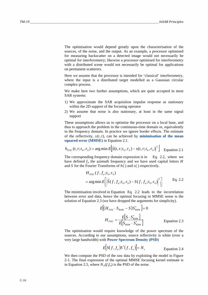
These assumptions allows us to optimise the processor on a local base, and thus to approach the problem in the continuous-time domain or, equivalently in the frequency domain. In practice we ignore border effects. The estimate of the reflectivity, s(t ,τ), can be achieved by minimisation of the mean squared error (MMSE) in Equation 2.1.
[ ]2000000 ),;,(),;,(ˆminarg),;,( ττττττ ttsttsEtthFOC −= Equation 2.1
The corresponding frequency domain expression is in Eq. 2.2, where we have defined f a the azimuth frequency and we have used capital letters H and S for the Fourier Transforms of h( ) and s( ) respectively.
⎥⎦⎤
⎢⎣⎡ −=
2
0000
00
),;,(),;,(ˆminarg
),;,(
ττ
τ
tffStffSE
tffH
aa
aFOC
Eq. 2.2
The minimisation involved in Equation Eq. 2.2 leads to the incorrelation between error and data, hence the optimal focusing in MMSE sense is the solution of Equation 2.3 (we have dropped the arguments for simplicity).
( )[ ] 0=−⋅ ∗RAWRAWFOC SSSHE
[ ]
[ ]∗
∗
⋅⋅
=RAWRAW
RAWFOC SSE
SSEH Equation 2.3
The optimisation would require knowledge of the power spectrum of the sources. According to our assumptions, source reflectivity is white (over a very large bandwidth) with Power Spectrum Density (PSD)
( ) ( )[ ] saa NffSffSE =,, * Equation 2.4
We then compute the PSD of the raw data by exploiting the model in Figure 2-1. The final expression of the optimal MMSE focusing kernel estimate is in Equation 2.5, where Nw(f ,fa) is the PSD of the noise.

_________________________________________________________ Focusing, interferometry and slope estimate
C-17
s
awN
ffNSAR
SARFOC
HHH
),(2 +=
∗
Equation 2.5
The result in Equation 2.5 is the well known MMSE Wiener inversion, that leads either to the matched filter, when Nw << Ns, or to the inverse filter, when Ns >> Nw. In any case, the focusing reference is phase matched to the SAR acquisition, so that the overall end-to-end transfer function has zero phase (linear, if we add the proper delay): that is the reason why SAR focusing for interferometry is usually defined as ‘Phase Preserving’.
In a conventional SAR, we expect a constant PSD for both thermal and quantisation noise, whereas the azimuth ambiguity is weighted by the antenna pattern giving a coloured noise. A conventional rectangular antenna of length L causes the spectral weighting:
( ) ( )⎟⎠⎞
⎜⎝⎛ −= DCaa ff
vLfG2
sinc2 Equation 2.6
The azimuth ambiguity is due to the folding of the spectra due to PRF: the PSD of SAR data, the first left and right ambiguities, and the expected ambiguity-to-signal PSD are plotted in Figure 2-2.
Figure 2-2: Azimuth Antenna Pattern in the frequency domain (dB) (continuous
line) together with its left and right replica, folded by azimuth sampling (PRF). The ambiguity-to-signal ratio is plotted as the dotted line.
We notice that for most of the azimuth bandwidth the signal is much larger that the ambiguity, so that the optimal focusing in Equation 2.5 is very close to the inverse filter. This is quite different form the matched filter used in RADAR detection and communications; in fact the matched filter comes out from the maximum likelihood optimisation for isolated targets, and not for a continuous distribution of scatterers. Finally, we observe that in most commercial Phase Preserving processors, proper spectral shaping windows are applied in order to reduce the side lobes in presence of non-stationary

TM-19 _________________________________________________________________________ InSAR Principles
C-18
targets (like strong point scatterers or man made artefacts). These shapes should then be equalised for interferometric processing on a nearly homogenous scene.
2.1.2 CEOS offset processing test The CEOS phase preserving test has been introduced to check the quality of the space-domain varying implementation of the processor. SAR processors usually approach a space-varying transfer function by block-processing, and adapting the processing parameters in each block. The ‘CEOS offset’ tests the self consistency of such approach, in particular checking that the same transfer function is implemented at a specific range and azimuth, disregarding the relative position with respect to the block [Bamler95A, Rosich96]:
“Process two SLCs from the same raw data set and with the same orbit, but offset by l00 lines in azimuth and l00 sample in range. The interferogram formed from these two properly coregistered SLCs should ideally have a constant phase of zero and thus reveals processor induced artefacts.”
The test must be passed with the following results:
• Mean of interferogram phase ≤ 0.1o • Standard deviation of interferogram phase ≤ 5.5o (corresponding to a
reduction in coherence ≤ 0.1 %) • No obvious phase discontinuity at the boundaries of processing blocks
The test does not provide a reference Doppler, however it is wise to perform it at the largest Doppler foreseen for the mission. Moreover, the azimuth shift should not be given when testing ScanSAR modes.
Clearly the test provides only a necessary condition, for example any range invariant operator would pass it, and the same for a one-dimensional operator. Hence, it is necessary to combine it with a measure of the actual focused quality.
We also notice that further self-consistency tests could be implemented, such as comparing the processing of blocks of different sizes.
2.2 Interferometric SAR processing So far we have considered the design of an optimal focusing processor as the one that provides the most consistent reconstruction of the source reflectivity. However, in processing a specific interferometric pair, some further processing specifically matched to that image pair can be performed to provide the best quality final interferogram.
The simplified design of the system and the processing in the interferometric case is shown in Figure 2-3. Here again we assume a distributed target, as we refer to conventional interferometry. We observe that the source reflectivity is affected by a noise contribution, namely ‘scene decorrelation noise’ that will not be noticed in processing a single channel (see Figure 2-1). With this warning in mind, we represent this contribution as an additive

_________________________________________________________ Focusing, interferometry and slope estimate
C-19
noise source. Scene decorrelation may arise from change in the scattering properties between the two acquisitions, from volumetric effects or baseline decorrelation [Zebker92]: for repeat-pass interferometry this may be indeed the strongest noise.
Figure 2-3: Schematic block diagram for the generation of a complex interferogram
in the single-baseline case. The scene decorrelation noise is not noticeable on the single image.
The SAR acquisition channels for master and slave are not identical to the single channel shown in Figure 2-1, as here we must account for the different acquisition geometry that interferometry looks for. Following the discussion in section 1.1.3 we need to replace the reflectivity s(t ,τ ) by its modulated version:
⎟⎠⎞
⎜⎝⎛ Δ−⋅=
⎟⎠⎞
⎜⎝⎛ Δ+⋅=
tfjtsts
tfjtsts
S
M
22exp),(),(
22exp),(),(
πττ
πττ
Equation 2.7
where M and S refer to the master and slave respectively.
We have approximated the case of a constant sloped terrain, leading to the total frequency shift Δf expressed in Equation 1.19 (notice that the equal repartition of the total spectral shift into two contributions of Δf /2 in each channel is purely conventional). The case of space-varying slopes will be approached in a later section.
2.2.1 Spectral shift and common band filtering (revisited)
The object of the processing block named: ‘spectral shift and common band filtering’ in the diagram of Figure 2-3 is to extract only those contributions correlated in both channels, and likewise to remove all the decorrelated contributions. Let us refer to the master and slave phase-preserving complex focused images as sM(t ,τ ) and sS(t ,τ ) respectively.

TM-19 _________________________________________________________________________ InSAR Principles
C-20
We again have to face the problem of an optimal estimate in the MMSE sense, but now the task is to filter the master instead of focusing, thus getting an image as close as possible to the slave:
),(*),(ˆ | ττ tsshts SMMMS ≈= Equation 2.8
where MSs |ˆ is the reconstruction of the slave image given the master, and hM is the reconstruction filter to be designed (the ‘spectral shift and common band’ block in Figure 2-3).
In the same way, a slave reflectivity would then be reconstructed from the master.
The design of filter hM is accomplished by minimising the MMSE in the bidimensional frequency domain:
⎥⎦⎤
⎢⎣⎡ −=
⋅=2
|
|
ˆminarg
ˆ
MMSHM
MMMS
SSEH
SHS Equation 2.9
This minimisation leads to the incorrelation between the error and data:
( )[ ] 0ˆ| =⋅− ∗
MMMS SSSE Equation 2.10
Eventually we derive the formulation of the reconstruction filter:
[ ][ ]∗
∗
=MM
MS
SSESSEH Equation 2.11
This filter keeps the most correlated information. However, Equation 2.11 does not hold for non-zero spectral shifts (Δf ≠ 0), i.e. it does not hold for different modulation of the sources that come out of the interferometric acquisition geometry (see section 1.1.3). In this case we have to shift the spectra of the two signals prior to correlating them, and this leads to the following result:
[ ][ ]
⎟⎠⎞⎜
⎝⎛ +
Δ+Δ−=
Δ−Δ+=
∗
∗
∗
s
awMaFOCM
NffNffH
aEM
aESaEM
SS
aSaM
ffH
fffHfffH
SSEfffSfffSE
H
),(),(2 2
1),(
),2/(),2/(
),2/(),2/(
Eq. 2.12
where: HEM and HES represent the end-to-end transfer functions (acquisition + focusing, as shown in Figure 2-1) of the master and slave channels respectively NwM(f ,fa) is the equivalent noise PSD on the raw master image HFOCM is the focusing transfer function of the master
Be warned that the inversion involved in Equation 2.16 is meaningful only in the bandwidth of the end-to-end transfer function (out of this band there is

_________________________________________________________ Focusing, interferometry and slope estimate
C-21
indeed no signal), or better in a smaller bandwidth to account for non-linearity of the on-board filter.
In a usual SAR system, the end-to-end transfer function is close to a band-pass in both range and azimuth, with the central frequency equal to the transmitted frequency f0 in range and to the Doppler centroid in azimuth. Therefore, the numerator in EquationEq. 2.12 has the fundamental role of keeping only the contributions in the common bandwidth (after providing spectral alignment), whereas the role of denominator is just to filter out-band noise.
2.3 DEM generation: optimal slope estimate Let us derive here the estimate of the spectral shift Δf , by assuming the 1-D case (along range). We notice that Δf is related to the ground range slope, hence this estimate is what interferometry looks for in DEM-generation oriented applications.
The Maximum Likelihood estimator of the interferometric phase has been derived in [Tebaldini05] for the case of a distributed target, and properly accounts for both the non-stationary local topography and the discrete (sampled) case. However, in the particular case of a constant slope we can get the same result by a minimising the squared error in the frequency domain.
Let us assume the MMSE estimate of the slave SLC, obtained by processing the master with the filter computed in EquationEq. 2.12. The error between the estimate and the given master image is:
( ))()(ˆ)( || ffSfSfE SMSMS Δ+−= Equation 2.13
We estimate the local spectral shift by imposing the minimisation of the integrated error, in the frequency domain:
dffWfEf MSMSHf)()(minargˆ
|2
|, ∫Δ=Δ Equation 2.14
where the whitening term WS|M(f) provides the optimal weight, that should be inversely proportional to the variance of the error itself, σ2
ESM(f).
The schematic block diagram of the optimal estimate of the frequency shift is drawn in Figure 2-4.

TM-19 _________________________________________________________________________ InSAR Principles
C-22
Figure 2-4: Schematic block diagram for (a) the interferometric model and (b) the optimal (MMSE) estimate of the local slope (or frequency shift, Δf)
The optimal expression of the weights is then computed as follows:
dffA
fA
ffSfSE
AfW
ESM
ESMSMS
MS
)(
)()()(ˆ)(
2
22
|
|
−∫=
=
⎥⎦⎤
⎢⎣⎡ Δ−−
=
σ
σ Eq. 2.15
Note that the scheme assumes all the spectral shift is in the slave image. Moreover we are considering the 1-D case (along range). The master and slave reconstruction filters, from Equation Eq. 2.12, become:
( )
( )s
wS
s
wM
ESES
aESaESSM
EMEM
aESaEMMS
HHffHfffH
H
HHfffHffH
H
σσ
σσ
+Δ−
=
+Δ+
=
∗
∗
∗
∗
1),(),(
1),(),(
|
|
Equation 2.16
where σwM, σwS, and σS represent respectively the standard deviation of the noise on the master image, the noise on the slave image, and the source reflectivity, and we assume that the inversion is applied only in the master and slave’s bandwidths.
The computation of the error variance, σ2ESM(f), can be performed by
exploiting the interferometric model, the error definition in Equation 2.13, and the master synthesis expressed by Equation 2.9 and Equation 2.16.
Eventually we achieve the result expressed in Eq. 2.17, where we have assumed the same transfer function for the master and the slave end-to-end channel, He(f).

_________________________________________________________ Focusing, interferometry and slope estimate
C-23
( ) ( )( ) ⎟⎟⎟
⎠
⎞
⎜⎜⎜
⎝
⎛
++
Δ−−+=
∗
22222
2
42222)()(
)(ESwSSwM
EESESwSESM
H
fHffHHf
σσσσσσσσ Eq. 2.17
This equation can be further rearranged to evidence the weighting factor γ , defined in Equation 2.18, which – not surprisingly – corresponds exactly to the coherence of the interferometric pair.
( )( )2222
42
SwMSwS
S
σσσσσ
γ++
= Equation 2.18
We eventually compute the whitening factor by combining Eq. 2.17 and Equation 2.18 and using them in Eq. 2.15 to get the final frequency shift estimator:
dffHffHfH
fHA
dffHffHfH
ffSfSfHfAf
EEE
E
EEE
SMSE
f
224
2
224
2
|2
)()()(
)(
)()()(
)()(ˆ)()(minargˆ
Δ−−=
Δ−−
Δ−−Δ=Δ
∗
∗Δ
∫
∫
γ
γ
Eq. 2.19
We can furthermore simplify this expression, by assuming that HE(f) = H0, constant in the whole range bandwidth, getting the result:
dfffSfSHffH
fAf MMS
Ef
2
|2
02
)()(ˆ/)(1
)(minargˆ Δ−−Δ−−
Δ=Δ
∗Δ ∫γ
Eq. 2.20
to be windowed in the range bandwidth. This expression needs to be completed with its symmetric contribution (the estimate of the slave from the master), as shown in Figure 2-4.
Let us focus on the whitening term (the first factor in the integral in Eq. 2.20). For each search frequency, fΔ , we assume that correlated
contributions come from f > fΔ , therefore we weight these contributions with the factor 1/(1–γ2) that is always > 1, and gets larger the higher the coherence. On the other side, the contribution outside the supposed common bandwidth, has unit weight. It is interesting to note that the Cramér Rao Bound would depend upon the width of the transition between the two regions (f < fΔ and f > fΔ ): a sharp transition (that would result from a wide extent of the data), would provide high accuracy, whereas a smooth transition (small range extent) would provide a coarse accuracy. [Tebaldini05] gives a simplification for γ2 << 1; in that case Eq. 2.20 leads to:
⎟⎠⎞⎜
⎝⎛ −Δ++Δ−−=Δ ∫∫Δ
dffSffSdfffSfSf MSMMMSf
2
|
2
| )()(ˆ)()(ˆminargˆ Eq. 2.21
where the two symmetric contributions have already been added.

TM-19 _________________________________________________________________________ InSAR Principles
C-24
This would be the ML estimate for low SNR, thus quite robust with respect to model errors.
2.4 Noise sources The impact of noise in interferometry is quite different from the single channel case due to the added source decorrelation, shown in Figure 2-3. In order to evaluate its impact with respect to the other contributions, we have evaluated the various signal-to-noise ratios for a typical ERS-Envisat case. More precisely, we have assumed:
• a typical Noise Equivalent σ0 of –24 dB [Laur98]; • a mean reflectivity σ0 = −10 dB (the 50% reference curve adopted for
Envisat ASAR); and • two different levels of scene decorrelation, roughly corresponding to ‘good’ (e.g. stable in time) and ‘very good’ cases (γ = 0.7 and γ = 0.95), this last achievable only on desert areas.
Results are plotted in Figure 2-5.
Figure 2-5: Ratio between Noise Power Spectrum and Signal PSD, estimated on the raw data, for the different kinds of decorrelation noise sources. Scene decorrelation
appears to be the dominant effect of scene coherence up to γ = 0.95.
Note that we have assumed that data has been processed with the inverse filter, so that both system noise (thermal and quantisation) and azimuth ambiguity appear rather high-pass. Even though for most of the azimuth bandwidth the major contributor seems to be the scene decorrelation, the
_________________________________________________________ Focusing, interferometry and slope estimate
C-25
best quality is simply achieved by maximising the ‘processed’ azimuth bandwidth, e.g. by performing antenna pattern deconvolution.
In conclusion, the inverse focusing reference (with some tapering at the bandwidth edges) is recommended for maximising interferometric quality in most cases (γ scene up to 0.95), whereas a more complex scene-dependent optimisation is required for highly coherent scenes.
The advantage of performing antenna pattern deconvolution, compared for example with the use of a flat amplitude reference, can be approximated to a 3 dB improvement in SNR, as by compensating for the antenna pattern we increase the processed Doppler bandwidth from ∼PRF/2 (the antenna –3 dB bandwidth) to ∼PRF.
2.5 Processing decorrelation artefacts So far, we have defined the optimal phase preserving focusing and interferometric processors by assuming perfect knowledge of the geometric and system-related parameters.
However, it may happen that, due to errors in these parameters or to the realisation of an approximate processor, the transfer function implemented in not exactly phase matched to the system. In these cases, the impact on the final quality can be expressed in terms of the coherence [Just94]. Let HSAR1, HSAR2 be the acquisition transfer function of the two interferometric channels (see Figure 2-1), and HFOC1, HFOC2 the two focusing operators, and HE1 = HIRF1⋅HFOC1, the end-to-end transfer function of channel 1 (similarly for channel 2). Coherence can be expressed directly in the frequency domain by means of Parseval identity [MontiGuarnieri96B, Cattabeni94]. If we assume a totally correlated target and we ignore noise we get the processor coherence contribution:
( ) ( )∫∫∫∫
∫∫=
aaSARaaSAR
aaSARaSARproc
dfdfffHdfdfffH
dfdfffHffH
22
21
*21
|),(||),(|
),(),(γ Eq. 2.22
This contribution should then be multiplied by the other decorrelation sources (temporal, geometric etc.) to get the overall coherence [Rodriguez92, Villasenor92].
In theory, the integrals should be extended to the common support between the two datasets, both in range and in azimuth, to account for the filtering expressed in Eq. 2.12, and the result would be space-varying. In practice we will evaluate the impact of distortions by assuming the full range and azimuth bandwidth.
We discuss here the cases of an error in the Doppler rate, and an error in the estimate of co-registering parameters.
TM-19 _________________________________________________________________________ InSAR Principles
C-26
2.5.1 Examples of decorrelation sources Let us assume that the phase artefact in SAR focusing is expressed by the (residual) pure phase transfer function Hd(f) = exp(j2πφ(f)) in both channels, one-dimensional in range. The coherence contribution can be estimated by exploiting Eq. 2.22, obtaining:
∫
∫
Δ+−Δ−=
Δ+Δ−=
dfffffjB
dfffHffHB ddproc
)))()((2(exp1
)()(1 *
φφπ
γ Equation 2.23
Note that no decorrelation results if the phase error is symmetric, or if the spectral shift is zero – whatever the distortion. As an example, an error in the replica quadratic phase coefficient leads to a defocusing, but not to a coherence loss, provided that the same error is applied to both channels.
In a general case, we can predict that the same phase distortion leads to no quality loss in azimuth, whereas it can give space-variant decorrelation (and phase bias) in range, according to the spectral shift.
However, if the phase distortion applies to one channel only, a decorrelation noise is introduced. This can be the case when a fixed replica is used to perform range focusing. Let us approximate the error as a pure quadratic phase, like in Equation 2.24, where k is the quadratic phase error.
),exp()/(rect )( 2jkfBffH = Equation 2.24
For ERS, we can expect a drift of ± 0.015% with respect to the nominal value ko = 7.5⋅10–12 rad/Hz2. The coherence can be estimated by series expansion of H(f), and assuming the worst case (no spectral shift), the correlation contribution of processing is expressed in Equation 2.25.
∫∫+
−
+
− ⎟⎟⎠
⎞⎜⎜⎝
⎛−+==
2/
2/
42
22/
2/
2
211)exp(1 B
B
B
Bproc fkjkf
Bdfjkf
BKγ
121601
242 kBjBkproc +⎟⎟
⎠
⎞⎜⎜⎝
⎛−≅γ Equation 2.25
This gives a phase bias arg(γproc) ≅ [(kB2)/12] = 0.2 rad and a decorrelation 1−|γproc| = 0.3. This decorrelation can be relevant for high quality processing.
Let now assume an azimuth misalignment Δt between the two images, e.g. a ‘residual’ TF, expressed in Equation 2.26 on one channel (and zero phase on the other).
2/2/)2exp(),(1
BffBffjffH
dcdc
xtxT
+≤≤−Δ≅ π
Equation 2.26
In Equation 2.26 we have assumed a Doppler Centroid Frequency fdc and a total bandwidth B (≤ PRF). This phase error leads to the coherence contribution shown in Equation 2.27.

_________________________________________________________ Focusing, interferometry and slope estimate
C-27
)2exp()(sinc
)2exp(1 2/
2/
tdct
Bf
Bf tproc
fjB
dffjB
dc
dc
ΔΔ=
Δ= ∫+
−
π
πγ Equation 2.27
The effect on the final interferogram is:
• a loss of quality, that depends on the coherence amplitude, i.e. a decorrelation: 1−| γproc| = 1−sinc( BΔt) ≅ [1/6]π2( BΔt)2 ;
• a phase bias, equal to the coherence phase, ∠γproc = 2πf dcΔt.
The decorrelation imposes a limit on the maximum tolerable misalignment, for example if we accept | γproc| < 0.95 (the best case assumed in Figure 2-5), we get Δt << 0.15 resolution cells. The phase bias is irrelevant only if it is constant over the processed data set (e.g. both misalignment and Doppler Centroid do not change), since the interferogram is usually known apart from a constant phase. Otherwise it can introduce significant phase artefacts: a misalignment of Δt = 0.15 /B would get a phase offset of 27o for a Doppler Centroid fdc = B /2. This is quite important if, for example, two different looks should be coherently averaged [MontiGuarnieri99B].
Other examples in literature may be found in [Just94, Cattabeni94].

____________________________________________________________________Advances in phase unwrapping
C-29
3. Advances in phase unwrapping
3.1 Introduction One of the most difficult problems in interferometry is the extraction of the absolute phases from the available wrapped values. In fact, in order to estimate topography and motion of the terrain we need the absolute phases, whereas the data are phase differences between the two images, in their principal interval ±π. Moreover, the wrapped phases are not available everywhere since we may have pixels without a significant radar return. And then, even if the phases are reliable, they may correspond to portions of the topography that are subject to alias and layover. This implies that, when using only one image pair, the operation of phase unwrapping may be subject to uncertainties that cannot be solved, unless we make hypotheses, usually statistical ones, on the structure of the underlying topography, or if we use additional information. In the section on multi-image phase unwrapping, we will see that this problem can have a unique solution if several image pairs with different baselines are combined. Obviously, this solution is available only where the target did not change during the entire span of the several surveys or it is seen simultaneously with multiple baselines and/or with multiple frequencies. Then, no hypothesis on the surface continuity is needed and the unwrapping can be carried out pixel by pixel. In this section we will approach the problem of phase unwrapping for image pairs, starting with simple cases (no or low noise, no aliasing) and then moving towards more difficult cases. The flat topography contribution is supposed to have been removed already.
In order to phase unwrap, we measure first the interferometric phase for all pixels and make an initial assumption that the measured values are reliable. Then, we add to each pixel phase value the integer multiple of 2π that is required to unwrap it. If we then scale the unwrapped phases to heights we get the topography in SAR coordinates. Any assignment of integers is acceptable, but then the topography may vary wildly from one pixel to the next. In other words, unlimited topographies exist, that honour the data.
Figure 3-1 shows an example of two-dimensional phase unwrapping on simulated data. The original topography is presented at left. The topography corresponding to the wrapped phase is presented at right.

TM-19 _________________________________________________________________________ InSAR Principles
C-30
Figure 3-1: Phase unwrapping. Left: absolute phase, named ψ .
Right: wrapped phase, named φ . Phase unwrapping regenerates the absolute phase, given the wrapped one (i.e. from right to left).
Problems of mono dimensional phase unwrapping are then exemplified in Figure 3-2: the unwrapping is carried out by supposing that the phase differences between neighbouring pixels are always under half cycle: whenever a phase difference greater than that is encountered, a cycle skip is surmised and compensated. In the case that the original phase difference is greater, this procedure generates an error.
1st plot: Absolute phase to be regenerated from the wrapped phase
2nd plot: Wrapped phase
3rd plot: Gradient of the wrapped phase. Absolute values larger than π are in red.
4th plot: Red dots wrapped to estimate the gradient of the unwrapped phase. This is incorrect when data are aliased, |Δψ |>π, as at sample 18.
5th plot: Reconstructed phase, obtained by integrating the gradient estimate from left to right.
6th plot: Notice the propagation of the error
Figure 3-2: Mono-dimensional phase unwrapping carried out by ‘integration of the estimate’

____________________________________________________________________Advances in phase unwrapping
C-31
3.2 Residues and charges To get a unique solution from a single pair of images, besides assuming there is no noise, we have to further suppose that the initial surface was sampled without alias. The actual phase differences between neighbouring grid points are then less than π or, in terms of topography, the elevation difference between neighbouring grid points is smaller than ha/2. This might be false in mountainous regions where layover is present in the resultant SAR data. We remember here that we can (and we should, as we shall see in the forthcoming sections) always remove the topography that is already known, to make the data as flat as possible. In other words, we should compensate for the local average slope of the terrain using a priori information of the topography, derived, for example, from lower resolution surveys. If there is no noise and no alias, then there is a true assignment of cycles to sum to the phases. The differences between the unwrapped phases of neighbouring pixels will then have a magnitude smaller than π and coincide with the Wrapped Phase Differences (WPD). The WPD are the measured phase differences (Figure 3-3) of two neighbouring grid points (thus in the interval ±2π) re-wrapped by adding ±2π (if necessary) so that they stay in the interval ±π. From the WPD we can, for no noise and no aliasing, retrieve the unwrapped values.
Figure 3-3: Left: The gradient is estimated by WPD. In the example, ψ i–1 = 3π/4; ψ i = –3π/4; the gradient is then Δψ= –6/4 π wrapped to WPD=–6/4 π +2π =π/2.
Right: In the 2-D case, the gradient is a vector with two components.
The problems with 2D phase unwrapping are exemplified in Figure 3-4 and Figure 3-5. The corruption of the WPD due to noise causes ambiguities.
Figure 3-4: A constant phase slope for the noiseless case. Left: wrapped phase.
Right: lines corresponding to zero crossings of the real and imaginary parts. These lines never cross (modulus ≠ 0). However, when the slope increases, the distance
between the lines decreases.

TM-19 _________________________________________________________________________ InSAR Principles
C-32
The problem is more easily understood in the continuous case. Suppose that we start from a discrete set of random complex numbers pij disposed on a square grid; then, we interpolate the real and imaginary parts of the pij’s, by convolving them, say, with a 2-D sinc function. We get a complex function p(x ,y) which is the sum of two continuous surfaces:
),Im(),Re(),( yxjyxyxp += Equation 3.1
The corresponding sampled surface is:
; ; ; ),( , Δ=Δ== jyixpyxp jijiji Equation 3.2
The phase ∠ p(x ,y) is well defined everywhere but at the points (say with coordinates (xr,yr)) where both Re(x ,y) and Im(x ,y) are zero, i.e. where the lines corresponding to the zeros of Re(x ,y) (∠ p(x ,y) = ±π/2) cross the lines corresponding to the zeros of Im(x ,y) (∠ p(x ,y) = π/2 ± π/2). These phase contour lines cross at the points (xr,yr) that are not necessarily on the sampling lattice [Schwartsman94]. Since the two continuous surfaces Re(x ,y) and Im(x ,y) are locally planar, only two possibilities exist, namely those circulating clockwise around (xr,yr) the phase either increasing or decreasing by 2π at each circuit (Figure 3-5). In the interferometric literature, following Goldstein who first studied this problem in the discrete case, we call these points residues, and charge refers to the sign of the curl of the phases. If we unwrap the phase by integrating the WPD following a closed path that encircles a residue, the result of the integration will be ± 2π. Then, the integration of the WPD is ambiguous if the phase contour lines cross. Therefore, a random phase distribution does not allow a unique solution for phase unwrapping. Depending on the integration path, we will find infinite solutions, all potentially acceptable and none of them being any more significant than any other.
Figure 3-5: Left: In the presence of noise, amplitude may go to zero, and two
neighbouring vortices with opposite charges are created. Right: If integration on a closed path embraces a vortex, a residual of ±2π results at each circuit. In fact,
whenever a zero line is crossed, the phase loses π/2.
If the phase contour lines cross, as will happen if the data are noisy enough, the vector field that has as components the WPD along azimuth and range is rotational. Then, the curl of this vector field is non-zero. If the continuous curl is non-zero and the total number of residues (both positive and negative) in a cell is non-zero, the discrete curl (the one measured on the discrete

____________________________________________________________________Advances in phase unwrapping
C-33
lattice, if the sampling frequency is sufficient) will also be non-zero, as will be seen in the next section.
3.2.1 Effects of noise: pairs of residues, undefined positions of the ‘ghost lines’
We consider now the case of low noise and no alias: for instance when the complex values pij correspond to a constant slope and therefore the phases increase progressively along a direction parallel to the slope. The lines that correspond to zero imaginary part and those corresponding to zero real part are interleaved as seen in Figure 3-5. The spacing of the lines corresponding to the zeros decrease with increasing slope. However, if no crossings exist then no residues appear, and the unwrapping problem has a unique solution (if the sampling grid is fine enough that alias is absent).
Let us now consider an example containing some complex noise. The lines corresponding to the zeros of the real and imaginary parts now start to wiggle and, with increasing noise, may cross in two neighbouring points. We have a pair of residues, where both Re(p)= Im(p)=0; in these two points the total sum of signal and noise has modulus equal to zero (Figure 3-5).
The charges of the two residues have opposite signs, as visible in the figure, since in one case the phase around the residue increases clockwise and in the other case anticlockwise. If the noise level is increased, more and more pairs of residues appear, always with opposite charges (Figure 3-6 and Figure 3-7) [Rosen00].
Figure 3-6: Residuals due to noise (SNR=8 dB) in the presence of a linear
increasing slope. Left: residuals, marked with ‘O’ and ‘+’ and contour lines of zero-real, zero-imaginary parts. Right: phase field. The density of the residuals
increases with the slope.

TM-19 _________________________________________________________________________ InSAR Principles
C-34
Now the unwrap problem is without a unique solution. If a phase integration path encircles only one of the two residues of any pair, 2π will be added (or subtracted) to the total phase and the final topography will depend on the integration path chosen. Any topography consistent with this noisy but continuous phase distribution cannot be continuous and should have an abrupt 2π discontinuity (e.g. a wall with height ha) connecting two residues with opposite charge.
From what we have seen, the number of pairs of residues will increase both with the local slope (that makes the lines of zeros closer to each other) and with noise (that makes the lines of zeros wiggle more) (Figure 3-7).
Figure 3-7: Residuals due to noise, as in Figure 3-6, but for different values of SNR:
left: 8 dB, right: 4.5 dB.
It is interesting to remark that the gradient of the phase change induced by the couple of residues is in the direction opposite to that of the slope. In fact, if the noise is small and the lines of the zeros of real and imaginary parts barely cross (say are tangent), the gradient will keep the same direction, change sign, and point down slope. Therefore the effect of noise will always be that of reducing the apparent amplitude of the slope. This result has been noticed and explained by Spagnolini [Spagnolini95] and Bamler [Bamler98B].
Let us now consider what happens when we sample on a grid. If the local topography is smooth and thus there is no alias, no ambiguity occurs in the noiseless case. The effects of noise will be pairs of residues, which will be close to one another if the noise is small. The residues will be revealed by computing the sum of the WPD around a square of four neighbouring pixels of the grid (the discrete curl) (see Figure 3-8).

____________________________________________________________________Advances in phase unwrapping
C-35
Figure 3-8: Gradient field in the neighbourhood of a dipole. Zero-real: continuous line. Zero-imaginary: dotted line. The gradient becomes very large approaching the
vortices and its direction is opposite to the local slope.
The discrete curl will be zero in normal situations, and ± 2π if the four neighbouring pixels encircle a point where we have a crossing of the lines that correspond to zero real and imaginary parts. It will again be zero if two residues are encircled that have opposite charge.
If now we wish to find a topography consistent with this phase distribution, i.e. to unwrap it, any integration path should not encircle any single residue, but only pairs with opposite charge. The simple way to do that is to connect neighbouring residues with opposite charges to lines that are not to be crossed. These lines, which have no physical meaning and their location totally undefined but for their end points, are called ‘branch cuts’ by Goldstein [Goldstein88] or ‘ghost lines’ by Prati [Prati90A]. The first name corresponds mainly to the hypothesis that the residues are due to noise and the branch cuts correspond to lines that are totally undefined, apart from their end points. The second name is related to alias in the topography due to coarse sampling, and in this case the actual position of the ghost lines is well determined physically but is undetectable from the experiment. This will be better seen in the next section.
For increasing noise levels, the possible topographies become more and more complex, with meandering walls with height ha that start from any positively charged residue and end in any negatively charged one. As said before, there is no way to ‘detect’ any ha discontinuity from the wrapped phases because the phases are not affected. In principle, a good way to unwrap is not to cross any branch cut; but again, their locations are totally undefined and therefore undeterminable from the phases. However, if there is no alias and the residues are due only to noise, and if the noise is small, it is reasonable to couple together neighbouring residues with opposite charge.
Increasing the level of the noise without limit, we get a very high density of residues. They are asymptotically one in three of the lattice points for sampled independent Gaussian noise on a square lattice. The density is one in four on a triangular lattice. Thus, if we have a rather flat surface with a lot

TM-19 _________________________________________________________________________ InSAR Principles
C-36
of phase noise, the best solution to smooth the phases before unwrapping, averaging them and thus removing the effects of neighbouring residues with opposite charges.
3.2.2 Effects of alias: unknown position of the ghost lines
In SAR geometry, it may happen quite often that the slope of a hill facing the radar has, between two adjacent pixels, a variation of the elevation with range higher than ha/2. Aliasing occurs since the WPDs are insensitive to any big elevation change and only measure the fractional part that is less than ha/2. Thus, we are obliged to consider the case of aliased surfaces: as with noisy data, we have residues and thus we have again a failure of any simple technique to determine the unwrapped phase. If we initialise the process at any given point of the image and then integrate the WPD from there to everywhere else, crossing an elevation change in the topography that is greater than ha/2 (a ghost line), we add 2π to the phases from this point on. Without alias and without noise, the sum of the WPD along any path would give us the same value as the unwrapped phase. In the case of alias, the discontinuity exists in the data but is visible only where it falls below ha/2. So, suppose we start from a valley and ascend to the top of a hill, as in Figure 3-9. If we access this point following a path that does not cross any such discontinuity, we shall find the correct altitude. If, while climbing the hill, we cross a discontinuity without knowing it, the final altitude will be short by ha.
Figure 3-9: Phase due to topography. Left: A strong gradient causes a phase discontinuity that may lead to alias,
depending on the baseline. Right: Wrapping a parabolic-like topography (shown in the shaded box). Pairs of residuals of opposite signs (marked with stars) are generated at the endpoints of the fringes.
How to avoid such a problem? We can detect the ends of the discontinuity since in these points the discrete curl of the WPD is non-zero. However, unless we use some a priori information of, say, geological nature, there is no way to tell where the discontinuity belongs, in between these two points (hence, the name ‘ghost lines’). In general, we may have many discontinuities in the image; we see only their end points, as in Figure 3-9

____________________________________________________________________Advances in phase unwrapping
C-37
(right), and we do not know which residue to connect with which other (even if we know that we have to connect residues of opposite charges to begin and end any discontinuity). As long as we place discontinuities along ghost lines of height ha beginning and ending at residues with the proper charge, we get topographies consistent with the phases. However, we have an unlimited number of solutions. In the case of alias, however, we can use a priori information. For example, alias is more likely in foreshortened areas, where the amplitude increases. The ghost line is likely to follow the direction of high amplitude lines [Prati90A].
3.3 Optimal topographies under the Lp norm We can find now different unwrapped phase distributions (topographies) optimal in the sense that each minimises a norm (Lp) of the error. Just as a reminder, we recall that in the case of a random variable z that corresponds to noisy measurements of the variable a , i.e.
ii naz += Equation 3.3
where z i, ni are the samples of the data and of the noise.
Then pa , the estimate of a optimal under norm p , is the number that minimises J :
[ ] ⎥⎦
⎤⎢⎣
⎡−== ∑
i
pi
apap zaJa ||minargminargˆ Equation 3.4
For p = 0, a is the value of the mode of the z i’s; for p = 1, their median; and for p = 2, their mean.
In the case of phase unwrapping, we can consider the policy of minimising the differences, raised to the power p , between the unwrapped phase differences along azimuth and range Δ(a)ψ i,j, Δ(r)ψ i,j corresponding to the chosen topography, and the WPD ji
aw ,
)( φΔ , jirw ,
)( φΔ along the azimuth and range coordinates i , j . We minimise then [Ghiglia98]:
∑∑∑∑ Δ−−+Δ−−= ++i j
pi,j
rwjiji
pji
awjiji
i jpC | | | | )(
,1,,)(
, 1, φψψφψψ Eq. 3.5
Obviously the minimisation of such a figure of merit appears to be, for p ≠ 2, a formidable problem, with no guarantees of being unique and, even more important, no guarantees that the optimal solution will be significant. However, there are important implications of the formula that show the usefulness of such an approach.
3.3.1 L2, L1, L0 , optimal topographies There are two apparently trivial phase unwrapping methodologies of a noisy and aliased phase field that are easy to describe: the first is to scan the image progressively, say left to right and then top to bottom, and to sum the WPDs
TM-19 _________________________________________________________________________ InSAR Principles
C-38
along each scan line, and along the vertical for the first pixel of each line. We get a topography with positive and negative ‘walls’, i.e. ha elevation discontinuities, directed along the scan lines, that start at the residues, and most likely end at the boundaries of the image: a very unlikely topography indeed, but consistent with the data and not optimal under any norm. Then, we could scan the image in any another direction and we would get another topography, unlikely as well. It is very interesting to observe [Fornaro96, Franceschetti99] that the average of all these unlikely topographies yields the optimal solution under the norm L2. Apart from boundary effects, we would get the same result by minimising the mean square value of the differences between the WPD (range and azimuth) and the phase differences derived from the unwrapped phases (the topography). In other words, we get such a topography that the WPD are matched as far as possible in the least square.
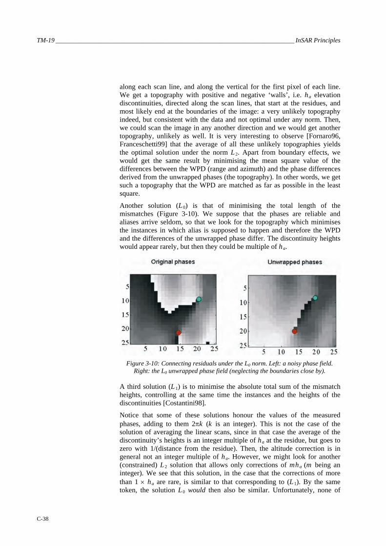
Another solution (L0) is that of minimising the total length of the mismatches (Figure 3-10). We suppose that the phases are reliable and aliases arrive seldom, so that we look for the topography which minimises the instances in which alias is supposed to happen and therefore the WPD and the differences of the unwrapped phase differ. The discontinuity heights would appear rarely, but then they could be multiple of ha.
Figure 3-10: Connecting residuals under the L0 norm. Left: a noisy phase field.
Right: the L0 unwrapped phase field (neglecting the boundaries close by).
A third solution (L1) is to minimise the absolute total sum of the mismatch heights, controlling at the same time the instances and the heights of the discontinuities [Costantini98].
Notice that some of these solutions honour the values of the measured phases, adding to them 2πk (k is an integer). This is not the case of the solution of averaging the linear scans, since in that case the average of the discontinuity’s heights is an integer multiple of ha at the residue, but goes to zero with 1/(distance from the residue). Then, the altitude correction is in general not an integer multiple of ha. However, we might look for another (constrained) L2 solution that allows only corrections of mha (m being an integer). We see that this solution, in the case that the corrections of more than 1 × ha are rare, is similar to that corresponding to (L1). By the same token, the solution L0 would then also be similar. Unfortunately, none of

____________________________________________________________________Advances in phase unwrapping
C-39
these solutions needs to be ‘true’ and statistics is the only tool available to evaluate the quality of the result.
Examples of phase unwrapping are given in Figure 3-11, Figure 3-12 and Figure 3-13.
Figure 3-11: An example of errors in Phase Unwrapping. Left: unwrapped phase
(error is encircled). Right: local slopes, estimated as the gradient of the unwrapped phase. Notice that the error is more evident in this image.
Figure 3-12: Example of 2-D phase unwrapping. (a) Noiseless unwrapped data; (b) Residuals, marked by white / black dots (depending on the sign) and zero-real, zero imaginary part contour lines. Only two residuals, due to topography, are found; (c) noisy wrapped phases; (d) distribution of residuals: of these, two are due to alias, the others to noise. Notice that the pair of opposite residuals tends to be aligned
orthogonal to the slopes, and that ‘–’ anticipates ‘+’ in positive slopes.

TM-19 _________________________________________________________________________ InSAR Principles
C-40
Figure 3-13: Examples of L 2 and L 0 norm phase unwrapping of the data in
Equation 3.11. (a) L 2 solution in the noiseless case: inconsistent with the data; (b) L 0 solution in the noiseless case: this is consistent with the data, albeit not
unique. (c) L 2 solution in the noisy case; (d) Phase error: it is a rotational field where the sources and sinks are in the residuals; (e) L 0 phase unwrapping, data
consistent; (f) difference between the L 0 solution and the original, noiseless topography: the difference is due to the noise. Large errors (only multiples of the
altitude of ambiguity h a) may exist, depending on the structure of the original data.
3.3.2 Slope estimates The previous techniques are designed to solve phase unwrapping problems in optics, Nuclear Magnetic Resonance, SAR interferometry etc. We will discuss now multi-pass SAR. Then, we have both alias and noise; in fact, the coherence on parts of the image might be quite low and the values of the interferometric phases very dispersed. Then, there is no other solution than making some sort of average and estimating the topography in a statistical sense. A reasonable approach is to hypothesise a locally planar surface and therefore the problem is reduced to that of slope estimation. Each slope corresponds to a sinusoidal behaviour of the fringes, uniform across the direction of the slope and with a frequency dependent on the slope. If the amplitudes of the interferometric signal were statistically uniform in the region of the slope, the maximum likelihood technique to estimate the slope in provided in section 2.3, a suboptimal but efficient technique could seek simply for the peak of the interferogram periodogram. In other words, we
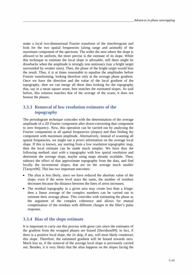
____________________________________________________________________Advances in phase unwrapping
C-41
make a local two-dimensional Fourier transform of the interferogram and look for the two spatial frequencies (along range and azimuth) of the maximum component of the spectrum. The wider the area where the slope is allowed to be uniform, the more precise is the estimate of its slope. While this technique to estimate the local slope is advisable, still there might be drawbacks when the amplitude is strongly non stationary (say a bright target surrounded by weaker ones). Then, the phase of the bright target would bias the result. Thus, it is at times reasonable to equalise the amplitudes before Fourier transforming, looking therefore only at the average phase gradient. Once we have the direction and the value of the local gradient of the topography, then we can merge all these data looking for the topography that, say in a mean square sense, best matches the estimated slopes. As said before, this solution matches that of the average of the scans; it does not honour the phases.
3.3.3 Removal of low resolution estimates of the topography
The periodogram technique coincides with the determination of the average amplitude of a 2D Fourier component after down-converting that component to zero frequency. Now, this operation can be carried out by analysing the Fourier components at all spatial frequencies (slopes) and then finding the component with maximum amplitude. Alternatively, instead of scanning all spatial frequencies, we might use a priori information on the average local slope. If this is known, say starting from a low resolution topographic map, then the local estimate can be made much simpler. We have thus the following method: start with a topography with low spatial resolution and determine the average slope, maybe using maps already available. Then, subtract the effect of that approximate topography from the data, and find locally the incremental slopes, that are on the average much smaller [Tarayre96]. This has two important outcomes:
• The alias is less likely, since we have reduced the absolute value of the slope; even if the noise level stays the same, the number of residues decreases because the distance between the lines of zeros increases;
• The residual topography in a given area may create less than a fringe: then a linear average of the complex numbers can be carried out to estimate their average phase. This coincides with estimating the phase as the argument of the complex coherence and allows for mutual compensation of the residues with different charges in the filter’s pulse response.
3.3.4 Bias of the slope estimate It is important to carry out this process with great care since the estimates of the gradient from the wrapped phases are biased [Davidson99]; in fact, if there is a positive local slope, the 2π skip, if any, will most likely counteract this slope. Therefore, the estimated gradient will be biased towards zero. Much less so, if the removal of the average local slope is previously carried out. Besides, it is very likely that the alias happens on the slopes facing the

TM-19 _________________________________________________________________________ InSAR Principles
C-42
satellite, where layover is likely. In these areas, the brightness is much higher due to the extent of the reflected energy that falls into a single resolution cell. Thus, it is reasonable to expect that most of the alias will occur in bright spots and, going from smaller to higher ranges, the aliased gradient will be short of 2π.
3.4 Analysis in the wave-number domain An interesting technique derived from the paper [Costantini99] is the following: measure the noisy phase gradient and evaluate the rotational component. In the frequency domain we evaluate the noisy gradients Ga(u ,v), Gr(u ,v) of the unwrapped phase field ψ (a ,r) (the inverse Fourier transform of P(u ,v)):
22 ]||[ ; ),(),(),( PnEvunvujuPvuG aaaa μ=+= Eq. 3.6
22 ]||[ ; ),(),(),( PnEvunvujvPvuG rrrr μ=+= Eq. 3.7
where (a , r) are the two coordinates (azimuth, range) (u , v) are the corresponding spatial frequencies in the transformed domain.
In order to simplify the notation, we assume continuous instead of sampled data.
P(u ,v) is the transform of the unwrapped phase (and, apart from a constant factor, the topography in SAR coordinates).
Ga, Gr are the transforms of the unwrapped phase (topography) gradients and apart from the noise due to wrapping these are equal to ju , jv times P(u ,v).
na, nr indicate the transforms of the noise mostly due to alias, i.e. of the walls with height equal to 2π or a multiple (proportional to multiples of ha that extend along range and/or azimuth), and that are visible only at their ends.
Simplifying the notation, we first find the 2D transform of the curl of the data as:
)( ravaR unvnjjuGjvGC −=−= Equation 3.8
Its inverse transform corresponds to the residues (mostly negative and due to layover). Then, where the absolute value of the discrete curl is greater than a threshold (π/4 in [Costantini99]) we add 2π to reduce it and re-compute the phase, and then iterate.
3.4.1 L2 optimisation in the wave-number domain Using this notation, we can also give the results of the L2 optimisation, which appeared in [Prati94B], since the unwrapped phase would be the optimal linear combination of the two noisy gradients:

____________________________________________________________________Advances in phase unwrapping
C-43
),(),(),(),(),( vuGvuRvuGvuAvuP ra +=)
Equation 3.9
Imposing orthogonality between data and reconstruction error we have:
( )[ ]( )[ ] 0
0*
*
=−
=−
r
a
GPPE
GPPE)
)
Equation 3.10
If we assume that the noise on the gradient is small and spectrally shaped as |P |, we find, consistently with [Ghiglia98], that if
μ r = μa = μ Equation 3.11
Then:
222
22 ; ),( ; ),( vujvvuRjuvuA +=Ω+Ω
−=
+Ω−
=μμ Eq. 3.12
In other words, if the noise is small, the Laplacian of the unwrapped phases to be estimated is equal to the Laplacian obtained from the WPD. In fact we get:
( ) ),(),(),(2 vujvGvujuGvuP ra −−=+Ω)
μ Equation 3.13
This is equivalent to the equations found in Equation B3.4, except that this is written in the frequency domain and Equation B3.4 is in the time domain.
Recalling that the noise on the gradient is shaped as walls in all directions, then:
21
Ω==
λμμ ar Equation 3.14
the coefficients become:
1
4
2
14
2
),( ; ),(λλ +Ω
Ω−=
+ΩΩ−
=jvvuRjuvuA Equation 3.15
Further, if we admit that with unequal sampling in azimuth and range the noise would not have equal power (i.e. mostly across range) then the coefficients become:
ar
arar
a
arar
r
vujvvuR
vujuvuA
μμμμμμ
μμμμμ
μ
>>++
−=
++−
=
; ),(
; ),(
22
22
Eq. 3.16
and therefore the reconstructed ‘walls’ would be mostly along azimuth and across range, giving results similar to what could be obtained using the technique described in [Costantini99].
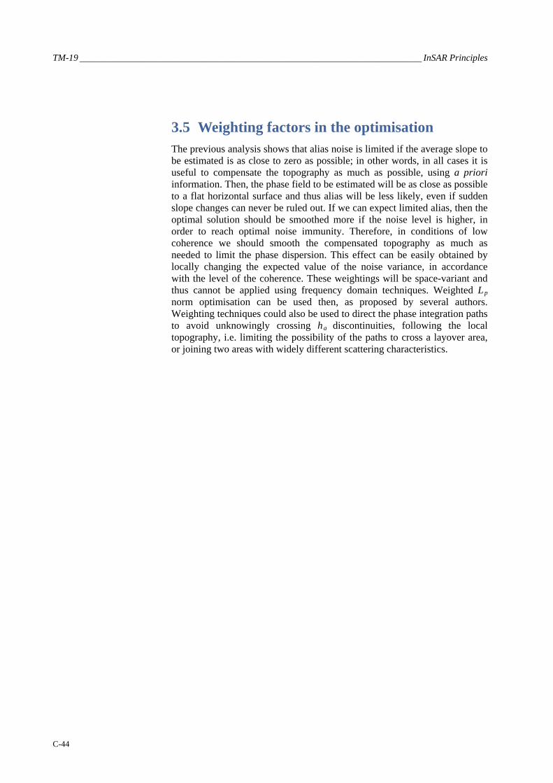
TM-19 _________________________________________________________________________ InSAR Principles
C-44
3.5 Weighting factors in the optimisation The previous analysis shows that alias noise is limited if the average slope to be estimated is as close to zero as possible; in other words, in all cases it is useful to compensate the topography as much as possible, using a priori information. Then, the phase field to be estimated will be as close as possible to a flat horizontal surface and thus alias will be less likely, even if sudden slope changes can never be ruled out. If we can expect limited alias, then the optimal solution should be smoothed more if the noise level is higher, in order to reach optimal noise immunity. Therefore, in conditions of low coherence we should smooth the compensated topography as much as needed to limit the phase dispersion. This effect can be easily obtained by locally changing the expected value of the noise variance, in accordance with the level of the coherence. These weightings will be space-variant and thus cannot be applied using frequency domain techniques. Weighted Lp norm optimisation can be used then, as proposed by several authors. Weighting techniques could also be used to direct the phase integration paths to avoid unknowingly crossing ha discontinuities, following the local topography, i.e. limiting the possibility of the paths to cross a layover area, or joining two areas with widely different scattering characteristics.

_____________________________Multiple image combination for DEM generation and ground motion estimation
C-45
4. Multiple image combination for DEM generation and ground motion estimation
4.1 Multi-baseline phase unwrapping for InSAR topography estimation
The theory of topographic mapping using SAR interferograms and the difficulties related to phase unwrapping of InSAR data have been presented in detail in recent review papers [Bamler98A, Massonnet98, Rosen00], and books [Franceschetti99, Ghiglia98]; here we address the multi-baseline technique, that removes the unwrapping problem in practice.
In the ideal case of no noise and no artefacts due to changes in the propagation medium, the interferometric phase φ of each pixel is proportional to the travel path difference and a function of the local topography. Since the quantity that can be measured from the interferometric image is not the phase ψ , but its wrapped (principal) value φ , the value of ψ has to be determined by means of a 2-D phase-unwrapping procedure. The quality of the final DEM is strongly dependent on this processing step. Conventional orbit determination is not precise enough for absolute phase retrieval and usually the final DEM is a map where all the values are computed with respect to a reference point P0 of known elevation z0. Therefore the datum used for DEM generation is not the phase φ of the generic pixel, but the unwrapped phase difference between P and P 0.
Once the phase unwrapping step has been carried out, it is possible to obtain the elevation of each pixel in the image. The phase to height conversion function g(Δφ) can be computed if the acquisition geometry is known. In general g(Δφ) is a non-linear relation involving, besides Δφ , the acquisition positions, i.e. the satellite orbits, the coordinates of the reference point, the range and azimuth variations between P and P 0, and the system wavelength.
In Figure 4-1 the area of interest is a small patch of ground around P0; the satellite trajectories are considered linear; and the phase to height conversion function can be well approximated by a linear relation:
( ) φφ Δ⋅+Δ⋅+Δ⋅=Δ=−=Δ CyBrAgzzz 0 Equation 4.1
where A , B , C are constant parameters, Δr = r(P) – r(P0) and Δy = y(P) – y(P0) (i.e. they correspond to the variations between the two pixels in range and azimuth direction respectively).
This linear approximation is useful because it highlights the main features of the acquisition geometry.
A depends on the off-nadir angle.

TM-19 _________________________________________________________________________ InSAR Principles
C-46
B is usually small but not negligible, since the orbits cannot be assumed parallel.
C is inversely proportional to the normal baseline Bn in y = y0 = y(P0). The height difference corresponding to a phase variation of one cycle is the so-called altitude of ambiguity h a:
θλπ sin2
2 0
n
Ma B
rCh =⋅= Equation 4.2
where θ is the antenna off-nadir angle rM0 is the distance between P 0 and the master trajectory (Figure 4-1).
y0P0
P
L
z
y
x
Bzi
Bxi
Bzf
BxfBn
M
S
H
rM0
Figure 4-1: InSAR geometry and symbols used
From the previous equation it follows that the greater the baseline, the greater is the interferometric phase difference between two points and the more difficult will be the unwrapping process due to the higher probability of phase aliasing. Moreover, geometric decorrelation strongly limits the SNR in high baseline interferograms [Gatelli94]. On the contrary, low baseline interferograms show good fringes, usually easy to unwrap, but with poor topographic accuracy [Ferretti99]. If more than one interferogram of the same region is available, phase unwrapping should be carried out simultaneously on the entire data set. The underlying idea of the multi-baseline approach is simple:
Interferograms are different measures of the same physical variable: the topography [Ferretti96B, Ferretti97]
If no a priori information about the topography is available, phase unwrapping of a single SAR interferogram is an ill-posed inverse problem. Even in high coherence areas, the presence of phase aliasing can produce serious artefacts on the estimated topography. If NI interferograms of the

_____________________________Multiple image combination for DEM generation and ground motion estimation
C-47
same region are available, with different baseline values, it is possible to combine the data to eliminate phase aliasing.
Theoretically it should be enough to have two interferograms with baseline ratios that are prime with respect to each other (their ratio is not a rational number) to be able to remove phase ambiguities (the Chinese remainder theorem). In practice, where data are noisy and baselines random, the use of multiple interferograms significantly increases the elevation ambiguity level. The use of Bayesian inference gives a rigorous framework for the estimation, taking into account possible a priori information about the DEM.
Let P0 be a point of known elevation (GCP: Ground Control Point). The target is then to compute the elevation of each point P in the area of interest with respect to P0. Let z(P) be the height variation between P and P0. This quantity can be considered as a random variable, its value can be estimated from the NI measures available. If f(z /Δφ i) is the probability density function (PDF) of the variable z conditioned to the wrapped phase value Δφ i (the apex specifies the interferogram used for the estimation), from the Bayes rule, if the measures are statistically independent, we have:
( ) ( )( ) ( )zf
fzf
Czf apNI
ww
NIwwNI
ww φφφφ
φφΔΔ
ΔΔ=ΔΔ
,.....,/,.....,1,.....,/ 1
11
Eq. 4.3
where C is a normalisation constant. The Maximum A Posteriori (MAP) estimate z of the variable z maximises this PDF. When the value of z is determined, it is easy to choose the multiple of 2π to be added to each interferogram: the correct value of the phase will correspond, in fact, to the height value nearest to the estimated one. In order to compute the conditional density we use the coherence maps associated with each interferogram. From the absolute value of the local coherence γ and the number of looks in the interferogram (the number of degrees of freedom in the estimate of Δφ), it is possible to compute the expression of the PDF of the interferometric phase and thus of the elevation. The conditional density function of the elevation for each interferogram is periodic with a different period (the altitude of ambiguity) dependent on the baseline. In each period the higher is the quality of the fringes (the coherence) the sharper is the histogram.
The product of the conditional densities shows a neat peak whenever the coherence is not close to zero and the baseline errors are not too high. The sharper the global peak, the higher the reliability of the results, i.e. the probability that the correct value of the height variation lies inside a given interval. In Figure 4-2 an example is shown of this kind of computation, where three interferograms with three different baseline values are considered.
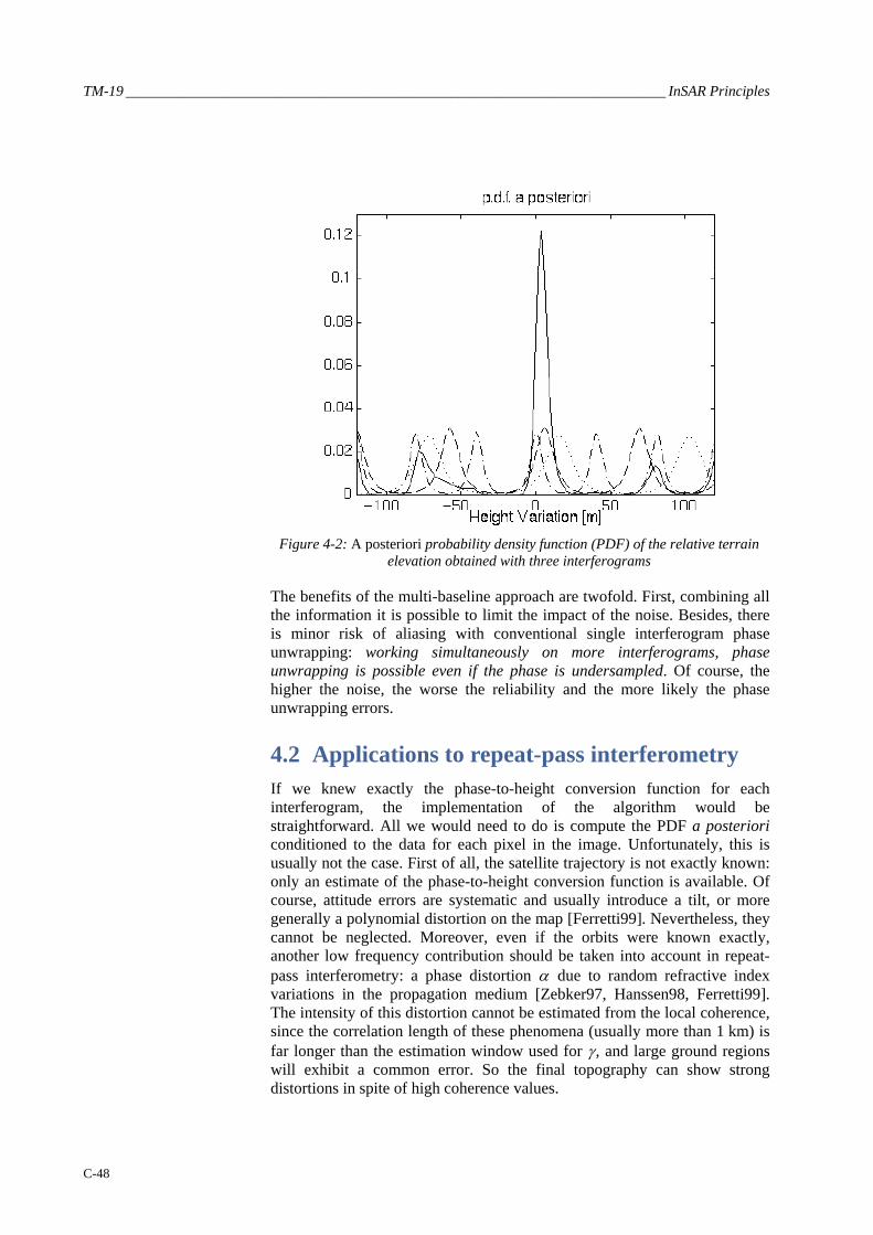
TM-19 _________________________________________________________________________ InSAR Principles
C-48
Figure 4-2: A posteriori probability density function (PDF) of the relative terrain
elevation obtained with three interferograms
The benefits of the multi-baseline approach are twofold. First, combining all the information it is possible to limit the impact of the noise. Besides, there is minor risk of aliasing with conventional single interferogram phase unwrapping: working simultaneously on more interferograms, phase unwrapping is possible even if the phase is undersampled. Of course, the higher the noise, the worse the reliability and the more likely the phase unwrapping errors.
4.2 Applications to repeat-pass interferometry If we knew exactly the phase-to-height conversion function for each interferogram, the implementation of the algorithm would be straightforward. All we would need to do is compute the PDF a posteriori conditioned to the data for each pixel in the image. Unfortunately, this is usually not the case. First of all, the satellite trajectory is not exactly known: only an estimate of the phase-to-height conversion function is available. Of course, attitude errors are systematic and usually introduce a tilt, or more generally a polynomial distortion on the map [Ferretti99]. Nevertheless, they cannot be neglected. Moreover, even if the orbits were known exactly, another low frequency contribution should be taken into account in repeat-pass interferometry: a phase distortion α due to random refractive index variations in the propagation medium [Zebker97, Hanssen98, Ferretti99]. The intensity of this distortion cannot be estimated from the local coherence, since the correlation length of these phenomena (usually more than 1 km) is far longer than the estimation window used for γ , and large ground regions will exhibit a common error. So the final topography can show strong distortions in spite of high coherence values.

_____________________________Multiple image combination for DEM generation and ground motion estimation
C-49
Atmospheric effects and baseline errors thus strongly reduce the effectiveness of the multi-baseline approach outlined above. In order to correctly unwrap the phase values, a good match between the topographic profiles coming from each interferogram is necessary. These low-frequency phenomena make a straightforward implementation of the multi-baseline approach unfeasible. The ‘resonance’ of the PDFs relative to the interferograms would become more and more unreliable for pixels more and more distant from the reference point P0.
The process has to be localised in order to remove these low wave number effects before expanding the procedure to wider and wider areas. In order to compensate for possible baseline errors and atmospheric distortion, the phase-to-height conversion functions are iteratively optimised as more and more points are unwrapped. A Root Least Mean Square (RLMS) optimisation is used to minimise the error between the elevation values obtained from each datum. Since the locally optimised baseline values compensate not only for orbit indeterminations but for atmospheric distortions too, they are called effective baselines. The need for optimisation procedures would make the implementation of the algorithm cumbersome and very time consuming. For that reason the processing is carried out at two different resolution levels. The image is divided into small blocks (of about 1 × 1 km) such that:
1) orbits can be considered linear; 2) phase distortion due to possible atmospheric effects can be considered
linear; 3) the phase to height conversion function can be well approximated, for
each interferogram, by a linear function:
iiiii DCyBrAz +Δ⋅+Δ⋅+Δ⋅=Δ φ Equation 4.4
where the apex specifies one of the NI interferograms. As already mentioned, all these variations are defined with respect to a reference point chosen inside each block. The reference point is a pixel having high coherence value in all the interferograms. The Di parameter compensates for phase noise on φ i(P0). Inside each block it is then possible to carry out a linear recursive optimisation, fast and effectively.
Results concerning two difficult test areas (Vesuvius and Etna) are presented below. The unwrapped phase maps were obtained by averaging the interferograms by a factor 5 in the azimuth direction (three effective looks were considered for PDF computation), maintaining full resolution data in slant range. The final resolution cell is about 20 × 20 m for flat terrain. Remember that the reconstructed unwrapped phase is identical to the original wrapped phase when unwrapped. In order to assess the reliability of the results, an a priori DEM of both test sites was used.

TM-19 _________________________________________________________________________ InSAR Principles
C-50
4.2.1 Example 1: the Vesuvius data set The multi-image reflectivity map (incoherent average of the co-registered SAR data) of the region around Mount Vesuvius is shown in Figure 4-3. The maximum height variation is 1281 m (from sea level to the top of the volcano). Seven Tandem interferograms were used, the baseline values ranging from 39 to 253 m. No a priori information was exploited during the processing.
Figure 4-3: Mount Vesuvius: multi-image reflectivity map

_____________________________Multiple image combination for DEM generation and ground motion estimation
C-51
Figure 4-4 shows the estimated topography after the first processing step. The blocks are still not unwrapped with respect to each other.
Figure 4-4: Estimated topography after the first processing step
The final DEM was computed using the seven unwrapped phase maps and the technique described in [Ferretti99]. In order to reduce baseline errors, the ESA precise orbits products (processed at GFZ/D-PAF, Oberpfaffenhofen) have been used to estimate the satellite trajectory relative to each image. A 3-D perspective of the final result is shown in Figure 4-5.
Figure 4-5: 3-D perspective view of the Mt. Vesuvius DEM

TM-19 _________________________________________________________________________ InSAR Principles
C-52
The error between the combined DEM and a reference (SPOT) topography (in SAR coordinates) is shown in Figure 4-6. White pixels correspond to areas not unwrapped (reliability under threshold). The error standard deviation is about 8 m. It should be noted that the available SPOT DEM has an estimated accuracy of 7 – 8 m, so multi-baseline InSAR data allow a precise estimation of the topographic profile.
Figure 4-6: Difference between the combined DEM and a reference (SPOT)
topography (in SAR coordinates)

_____________________________Multiple image combination for DEM generation and ground motion estimation
C-53
4.2.2 Example 2: The Etna data set The second example shown is the region around Etna. Eight interferograms were used. The area selected is about 30 × 30 km. As usual, the images were averaged only by a factor of five in the azimuth direction (Figure 4-7).
Figure 4-7: Mt. Etna: multi-image reflectivity map
An example of a reliability map generated by the multi-baseline phase unwrapping software is shown in Figure 4-8, while the best coherence map of the Etna data set is shown in Figure 4-9 for comparison.
Figure 4-8: Reliability map generated by the multi-baseline phase unwrapping
software. White=reliable; Black=unreliable.
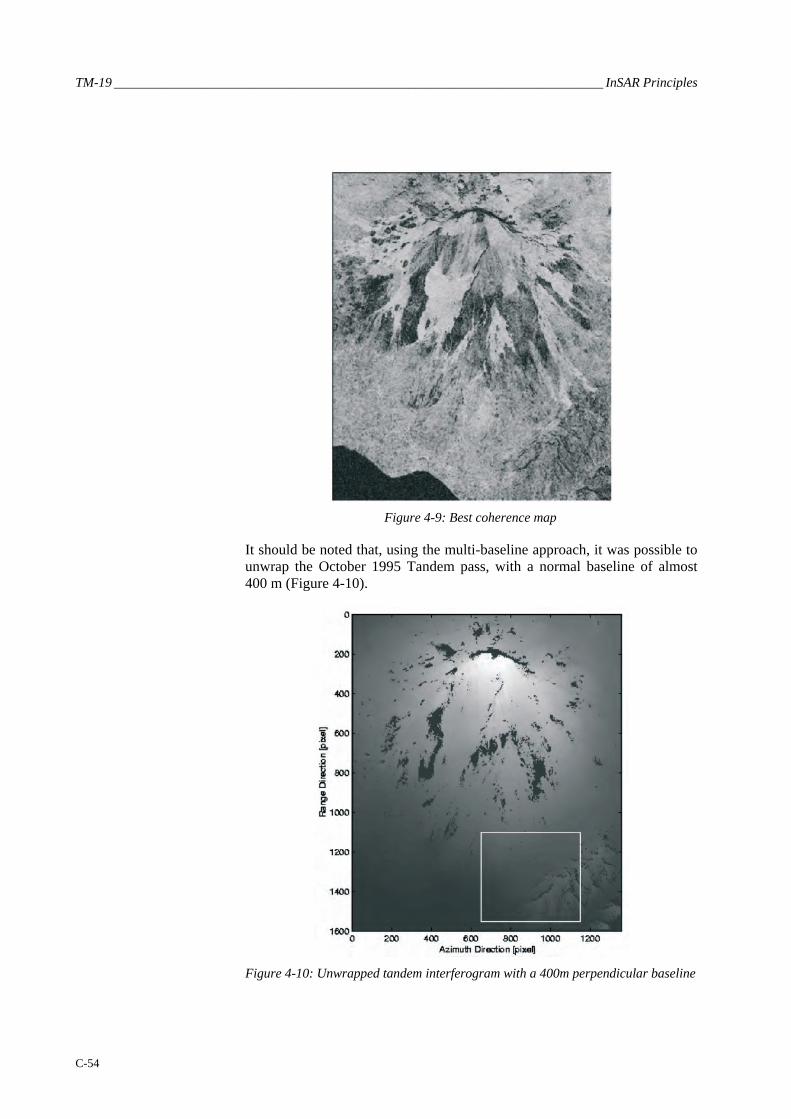
TM-19 _________________________________________________________________________ InSAR Principles
C-54
Figure 4-9: Best coherence map
It should be noted that, using the multi-baseline approach, it was possible to unwrap the October 1995 Tandem pass, with a normal baseline of almost 400 m (Figure 4-10).
Figure 4-10: Unwrapped tandem interferogram with a 400m perpendicular baseline

_____________________________Multiple image combination for DEM generation and ground motion estimation
C-55
The difficulties related to the unwrapping of this high baseline interferogram can be appreciated by analysing Figure 4-11, which shows a close up of the wrapped interferogram.
Figure 4-11: Close up of the wrapped interferogram with a 400m perpendicular
baseline
A perspective view of the final DEM, obtained from the combination of all the unwrapped phase data [Ferretti99], is shown in Figure 4-12.
Figure 4-12: Perspective view of the reconstructed Etna DEM

TM-19 _________________________________________________________________________ InSAR Principles
C-56
In order to assess the reliability of the final estimated topography, Figure 4-13 shows the error histogram with respect to a reference DEM provided by IPGP (estimated accuracy 4 m). The error standard deviation (computed for unwrapped pixels) is 7.5 m.
Figure 4-13: Elevation error histogram with respect to a reference DEM provided
by IPGP i(estimated accuracy 4 m)
4.3 The ‘Permanent Scatterers’ technique One of the main difficulties encountered in differential InSAR (DInSAR) applications is temporal and geometric decorrelation. The main goal of this section is the identification of single pixels (called Permanent Scatterers, PS) that are coherent over long time intervals and for wide look-angle variations [Ferretti00, Ferretti01]. This allows one to use many or all ERS acquisitions relative to an area of interest. In fact when the dimension of the PS is smaller than the resolution cell, the coherence is good (the speckle is the same) even for image pairs taken with baselines greater than the decorrelation length. On those pixels, sub-metre DEM accuracy and millimetric terrain motion detection can be achieved, even if the coherence is low in the surrounding areas. Reliable elevation and deformation measurements can then be obtained on this subset of image pixels that can be used as a ‘natural’ GPS network.
The mathematical framework for this kind of estimation is relatively simple. Let us suppose that N+1 ERS SAR images of the area of interest are
i Institut de Physique du Globe de Paris

_____________________________Multiple image combination for DEM generation and ground motion estimation
C-57
available. Data are first co-registered on a unique master, and a DEM of the area is estimated starting from low temporal baseline pairs [Ferretti99]. Next, N differential interferograms between all SAR images and the master are computed. After DEM compensation, the residual phase of interferogram i is:
itopoiiTii nr _4 εαλπφ +++= Equation 4.5
where λ is the system wavelength, α i the atmospheric phase contribution, ni the decorrelation noise, ε topo_i the phase contribution due to possible errors in the DEM (proportional to the normal baseline of each image Bn_i, and rTi is the possible target motion in the direction of the satellite line-of-sight.
The first term in Equation 4.5 can then be written as follows:
NLiviNLiirTi vCTvr μμλπ
λπ
+=+=44
Equation 4.6
where v is the unknown component of the mean target velocity in the direction of the line of sight, μNL is the phase term due to a possible non-linear target motion Ti is the temporal baseline between the master acquisition and the generic i-th slave image.
Since we have N differential interferograms of the same area with different temporal and geometric baselines, we finally write, for each pixel, a linear system of N equations and two unknowns:
vCC vizzii += εφ Ni ....1= Equation 4.7
Where: ε z is the DEM error Czi is proportional to Bn_i
The problem would be linear if we knew the unwrapped phase values. However, using a simple periodogram (albeit with an irregular sampling of the two dimensions: baselines and time) we can estimate both the residual elevation and the mean line of sight velocity, provided that the signal-to-noise ratio is high enough.
Actually the Linear Phase Residues (LPR) wi (i.e. phase data after linear detrending in temporal and spatial baseline) are the sum of three contributions: atmospheric components (Atmospheric Phase Screen – APS) of the master and the slave acquisitions, noise, and non-linear motion:
iiNLirvizziii nvCCw ++=−−= αμεφ Equation 4.8
Since μNL, α and n are independent random variables, the residual phase variance σ2
w is the sum of three contributions: σ2μ NL, σ2
α, σ2n. As a matter
of fact, a proper estimation of target motion and elevation is possible only if

TM-19 _________________________________________________________________________ InSAR Principles
C-58
σ2w is low. To this end, the analysis is carried out in two steps. First a subset
of image pixels is selected using the coherence maps of the area of interest: only locations of highly coherent targets are retained (low σ2
n). If now we consider a pair of targets not too far apart (distance less than, say, 1 km), it is usually possible to estimate Δv (relative mean velocity) and Δε z (relative elevation error) with a high degree of accuracy. In fact, low distance implies low variance of the atmospheric component: for points less than 1 km apart, values of σ2
α less than 0.1 rad2 are common. Moreover, the motion of neighbouring pixels is usually correlated. If this hypothesis is verified, σ2μ should be low as well. Estimation of (v , ε z) is then obtained by integrating the values of (Δv , Δε z) previously estimated from pairs of neighbouring pixels. Following this approach, we can actually unwrap the differential interferograms. In fact, if the condition |wi|<π is satisfied, we can easily recover the unwrapped phase differences Δϕ i between pairs of neighbouring pixels and then integrate them all over the sparse grid of PS candidates.
We can summarise the results as follows. Phase unwrapping of differential interferograms characterised by high geometrical and temporal baseline is possible only on a sparse grid of targets, previously selected as PS Candidates (PSC), and using a multi-image approach. The mathematical framework is easier if the constant velocity model can be applied. However, this hypothesis is not a real constraint and the technique can cope with non-uniform target motion, provided that the PS density and coherence is high enough (low σ2
w). Phase differences are unwrapped taking advantage of the estimated values of relative velocity Δv and relative elevation Δε z of each pair of scatterers. Phase data are then integrated using one of the techniques used for unwrapping regularly sampled data.
4.3.1 Space-time estimation Once phase data are unwrapped, it is possible to estimate the signal of interest by using an optimum filter, and properly weighting the data vector. In general, we may be interested in estimates at unmeasured points and instants too (interpolation and/or prediction). It should be noted that the optimum filter is space and time variant.
The key point for optimum filtering is the estimation of the correlation values. While expression of the correlation matrix of the atmospheric component can be obtained from Kolmogorov theory, a statistical description of the local displacement field can be very difficult to achieve.
Basically, this choice should reflect our knowledge about the physical phenomenon we are dealing with. If a model is available, parameters and expression of the correlation matrix assume a specific physical meaning. If no a priori information is available about the displacement field of the area of interest, a possible approach that can be adopted is the whitening of the time series of the Linear Phase Residues (LPR) samples. Once the residual phases of the PS Candidates have been obtained (data compensated for the estimated DEM errors and the mean velocity field), we can start looking at their temporal evolution, to check for subsidence leakage. The time-smoothed component should be considered as an estimation of the non-

_____________________________Multiple image combination for DEM generation and ground motion estimation
C-59
uniform motion contribution. Atmospheric Phase Screen (APS) estimation is then carried out to spatially smooth the time high-pass filtered LPR data.
To make it simple, we can for each pixel carry out a temporal smoothing using a triangular filter and remove the low pass component. However, seasonal effects can be removed from the data by using a band-pass filter. Phase residuals are then spatially filtered. After estimation and removal of all the APS superimposed on the data, we can finally estimate the motion of each pixel in the image and identify more PS’s. In fact the PSC set is just a rough estimation of the PS set since isolated coherent targets are not detected due to the space average used for coherence estimation.
4.3.2 Subsidence in Pomona An interesting case of subsidence, studied using differential interferometry and other techniques, is found in Pomona, California [Peltzereos]. 41 ERS images were obtained with the same track and frame (Track: 170. Frame: 2925). All were resampled on the same master acquisition (ERS-2, 6 April 1996) and 40 interferograms were obtained. Figure 4-14 shows the incoherent average of all the data (close up of Los Serranos area): due to the high number of looks, the radiometric quality of this image is comparable to that of an optical one. Using four Tandem pairs, we also determined a reference DEM (approximately 10 m accuracy, also limited by building effects) of the area of interest using the wavelet approach, and the corresponding phase was removed from each single image.
Figure 4-14: Geocoded multi-image reflectivity map of the test site (close up of Los Serranos area). The high radiometric quality is due to the incoherent data average
After the initial selection of the Permanent Scatterers set (about 3 PS/km2 were identified), phase increments between each PS and all the others less than 1 km away were estimated using the periodogram technique. To illustrate this approach, Figure 4-15 shows the temporal distribution of the takes together with their normal baselines, referred to the master image.

TM-19 _________________________________________________________________________ InSAR Principles
C-60
Figure 4-15: Space-time distribution of the available data. The bidimensional
sinusoid represents the phase contribution for a LOS velocity of 2 cm/y and a DEM error of 5 m.
The range of normal baselines is about +/– 1100 m, while the maximum temporal baseline is more than 6 years. If a PS had a Line Of Sight (LOS) velocity of, say, 2 cm/y and a residual elevation difference of 5 m with respect to a neighbouring scatterer, considered as a reference, its phase variations as a function of time and baseline would be a 2D sinusoid, also represented in Figure 4-15. If now we accept, temporarily, the hypothesis of constant LOS velocity of each pixel, then using a periodogram we can estimate both the residual elevation and the LOS velocity difference of the pixels. As already mentioned, this operation was carried out for all PS pairs less than 1 km apart, thus removing the effects of the residual elevation with respect to the average DEM and of the LOS velocity, and estimating the unwrapped phase values.
After estimation of both elevation and mean velocity of the targets, time series analysis of the phase residues in correspondence with each PS was carried out. The target is to identify possible non-linear motion contributions. APS’s were then interpolated on the original regular grid and removed from each datum. It should be noted that each APS is actually the difference of the atmospheric component of the slave image and the APS of the master acquisition. Averaging the 40 APS’s it was possible to get an estimation of the master contribution and then of each single contribution. An example of estimated APS is shown in Figure 4-16.

_____________________________Multiple image combination for DEM generation and ground motion estimation
C-61
Figure 4-16: Example of APS estimated for 6 April 1996. The APS has been superimposed on the multi-image reflectivity map of the area. APS standard
deviation is 0.86 rad.
Figure 4-17: Pomona: estimated displacement field in cm relative to the time
interval a) June 1992: February 1994; b) interval June 1992: September 1995; c) interval June 1992: May 1997; d) June 1992: January 1999. Colour scale has been saturated for visualisation purposes (+/– 12 cm). Contour lines step: 2.5 cm
After APS removal it is possible to estimate not only the mean velocity field of the area but a displacement field as a function of time, possibly interpolating the displacement maps on a regular temporal grid. Here we

TM-19 _________________________________________________________________________ InSAR Principles
C-62
report a sequence of four spatial maps corresponding to four equally-spaced time intervals (Figure 4-17).
The non-linear motion behaviour is reflected in the change of shape of the contour lines. A perspective view of the displacement field of Figure 4-17 is also shown in Figure 4-18. Maximum positive and negative displacements are +6 and –20 cm, respectively.
Figure 4-18: Perspective view of the displacement field relative to June 1992:
January 1999. Minimum negative value: –20 cm. Maximum positive displacement: +6 cm.
4.3.3 Ground slip along the Hayward fault The velocity field across the Hayward fault in California has been estimated by exploiting 55 ERS images acquired between June 1992 and November 1999 and processed with the Permanent Scatterers technique.
The PS density in the area is very high (over 200 PS/km2), so that the estimated LOS velocity field looks continuous in Figure 4-19. The relative dispersion of the velocity values in the two areas separated by the fault is lower than 0.4 mm/y. The stepwise discontinuity of about 2 mm/y in the average deformation rate can be identified easily and the hanging wall of the fault can be located with an accuracy of a few tens of metres.
In order to minimise interpolation artefacts, data are reported in SAR coordinates (range, azimuth) rather than in geographical coordinates. The sampling step is about 4 metres both in slant range and azimuth (ERS images have been interpolated by a factor of two in range direction). The radiometric quality of the image has been strongly improved by computing the incoherent average of the data.

_____________________________Multiple image combination for DEM generation and ground motion estimation
C-63
Figure 4-19: (a) Estimated LOS velocity field across the Hayward fault. (b) Close-up on cross section AA'.
(c) LOS displacement rates relative to the PS along section AA'.
4.3.4 Seasonal deformation in the Santa Clara Valley The PS technique can be exploited to identify seasonal deformation phenomena. As an example, the temporal analysis of the PS identified in the Santa Clara Valley (California) showed seasonal behaviour of the deformation due to the periodic water level variation, affecting an area limited by two known seismic faults.
The amplitude of this almost sinusoidal ground deformation is shown in Figure 4-20. Here, the border lines of the area affected by the seasonal deformation correspond to known seismic faults and are clearly visible on the colour image.

TM-19 _________________________________________________________________________ InSAR Principles
C-64
Figure 4-20: Map showing the amplitude of the seasonal ground deformation in the
Santa Clara Valley (CA)
The typical behaviour of a PS in the area affected by seasonal motion is shown in Figure 4-21. In this analysis 46 ERS images, from May 1992 to September 2000, have been used.
Figure 4-21: Typical behaviour of a PS in the area affected by seasonal motion
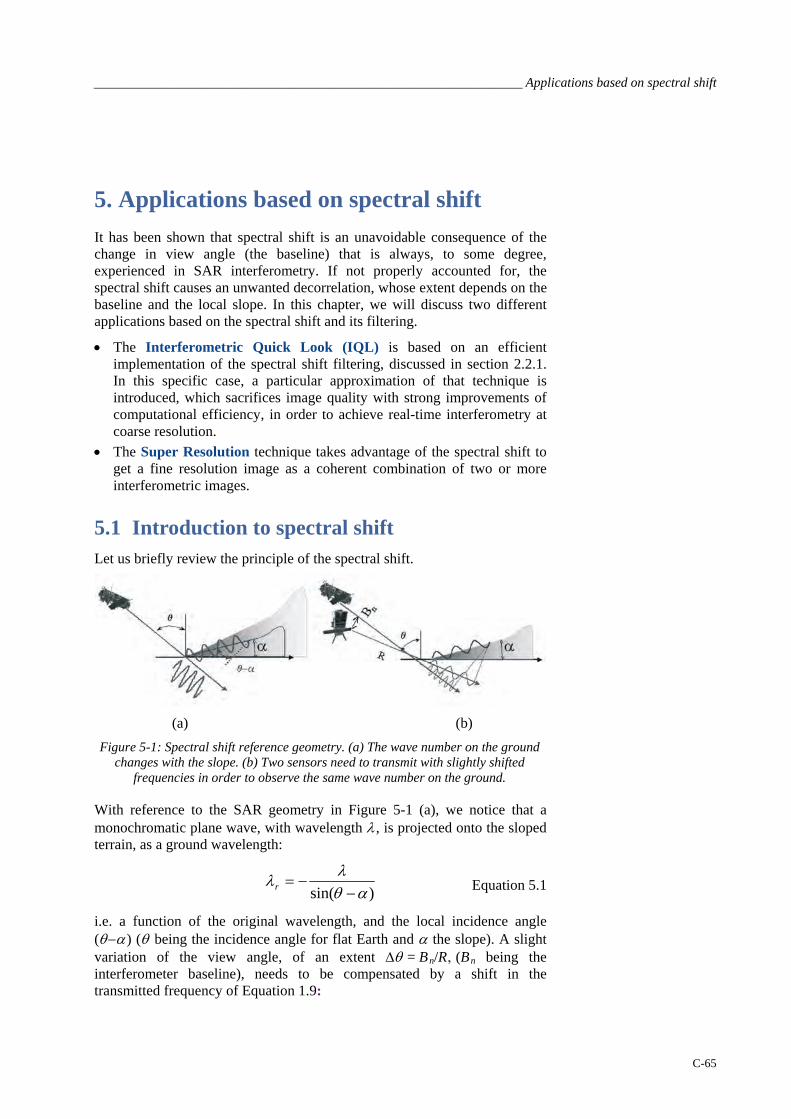
________________________________________________________________ Applications based on spectral shift
C-65
5. Applications based on spectral shift It has been shown that spectral shift is an unavoidable consequence of the change in view angle (the baseline) that is always, to some degree, experienced in SAR interferometry. If not properly accounted for, the spectral shift causes an unwanted decorrelation, whose extent depends on the baseline and the local slope. In this chapter, we will discuss two different applications based on the spectral shift and its filtering.
• The Interferometric Quick Look (IQL) is based on an efficient implementation of the spectral shift filtering, discussed in section 2.2.1. In this specific case, a particular approximation of that technique is introduced, which sacrifices image quality with strong improvements of computational efficiency, in order to achieve real-time interferometry at coarse resolution.
• The Super Resolution technique takes advantage of the spectral shift to get a fine resolution image as a coherent combination of two or more interferometric images.
5.1 Introduction to spectral shift Let us briefly review the principle of the spectral shift.
(a) (b)
Figure 5-1: Spectral shift reference geometry. (a) The wave number on the ground changes with the slope. (b) Two sensors need to transmit with slightly shifted
frequencies in order to observe the same wave number on the ground.
With reference to the SAR geometry in Figure 5-1 (a), we notice that a monochromatic plane wave, with wavelength λ , is projected onto the sloped terrain, as a ground wavelength:
)sin( αθλλ
−−=r Equation 5.1
i.e. a function of the original wavelength, and the local incidence angle (θ−α) (θ being the incidence angle for flat Earth and α the slope). A slight variation of the view angle, of an extent Δθ = Bn/R , (Bn being the interferometer baseline), needs to be compensated by a shift in the transmitted frequency of Equation 1.9:

TM-19 _________________________________________________________________________ InSAR Principles
C-66
( )αθθθ
θ −Δ
−=Δ∂∂
=Δtan
fff Equation 5.2
This fact is shown in Figure 5-1(b). As already stated in chapter 1.1, interferometry is made possible by the actual finite bandwidth of the SAR system. As an example, the value of spectral shift has been plotted in Figure 5-2 as a function of the ground slope, for three different baselines. In the example, the baseline value of 1000 is defined as ‘critical’ since this would introduce a spectral shift, for a flat terrain, equal to the system bandwidth: fringes will vanish for larger baselines.
Figure 5-2: Spectral shift has been plotted as a function of the terrain slope,
starting from back-slope (on the left) ending to the fore-slope, on the right. The ERS geometry was assumed, and three plots are drawn for different normal baselines. Dashed areas correspond to shadow and layover. The dark stripe in the middle marks the frequencies within ± the system bandwidth: when the spectral shift
exceeds that bandwidth, no correlated return is given.
The capability of getting interferometry over steep fore-slopes is thus linked to the amount of fractional bandwidth available. The fact is shown in Figure 5-3, where the common spectral components have been emphasised by the dark shading. If these components are selected by properly filtering the Master and Slave image, the spectra cross-correlations caused by the interferometric beat will result in an impulse, that is a linear phase in the time domain, e.g. the interferometric fringe represented in the plot of Figure 5-3 (on the right).

________________________________________________________________ Applications based on spectral shift
C-67
Figure 5-3: The master and slave image reflectivity are shifted by an amount that depends on the baseline. Their common spectral components (shaded in the first
three plots on the left) are used for interferometry (top right). The other components can be combined to reconstruct a ‘wide bandwidth’ reflectivity, hence a super-
resolution image (bottom left).
As a different and complementary application, the common and non-common spectral components can be added coherently to provide a large bandwidth, hence a super resolution image (see Figure 5-3 on the right).
5.2 Interferometric quick look (IQL) IQL represents a complete interferometric processor intended to get medium resolution STRIPMAP interferograms with quite small computational complexity. The processor exploits the spectral shift principle in order to halve the data rate with only a moderate loss in the final quality. This idea, first expressed in literature in [MontiGuarnieri93, Gatelli94], was developed by Politecnico di Milano into a full processor, to be installed at ESA facilities for browsing purposes [Walker98].
The processor reduces the ‘computing’ costs (time, memory, disk-space) by moving the ‘spectral shift & common band filtering’ step, usually performed on the azimuth focused images (see chapter B2) at the level of raw data, i.e. as the first step of the interferometric processing chain. This is done by range half-band filtering and decimation. Usually decimation implies a loss of information; however, in this case, the range filters are tuned to the spectral shift (for flat Earth) so that most of the information removed would have contributed as noise in the final interferogram. According to Figure 5-2, a spectral shift of ~9 MHz (half of the sampling bandwidth) corresponds to a baseline of ~500 m (for flat terrain). When the interferometric baseline is 500 m, the quality available by the IQL will be close to that of the full

TM-19 _________________________________________________________________________ InSAR Principles
C-68
resolutionii. For smaller baselines, the half-bandwidth filtering results in some loss of quality with respect to a full resolution processing.
Besides range spectral shift, the IQL implements an efficient azimuth common band filtering (see chapter B1), once again applied directly to the raw data. This filtering is simply implemented by means of an N = 8 channel polyphase and DFT filter bank [Fliege94], that divides the raw data into eight azimuth looks, of which three are discarded and the other kept. Such processing is well suited to the ERS Tandem mission, which experiences a Doppler Shift of 300 Hz (~ 1/6 of the PRF).
The joint use of this unconventional scheme for range subsampling and azimuth look formation provides the following advantages:
1) the computing costs are reduced by a factor ~3 due to data decimation, 2) all the known advantages of SAR multi-look processors in terms of
parallelism, scalability and efficiency have been achieved, and 3) the SNR is enhanced, thus improving performances of the required
parameter estimates.
The IQL implementation also integrated several ‘tricks’ to gain efficiency, like the exploitation of small, optimised kernels for image co-registration, and an original, quick-and-dirty algorithm to compute coherence maps [MontiGuarnieri97].
An overview of the whole algorithm is provided in the schematic block diagram in Figure 5-4; more details will be found in the journal paper [MontiGuarnieri99B].
Figure 5-4: Schematic block diagram of the IQL processor
ii Note that the processor actually performs a spectral shift filtering tuned for flat
Earth, which is not the best choice on a sloping terrain.
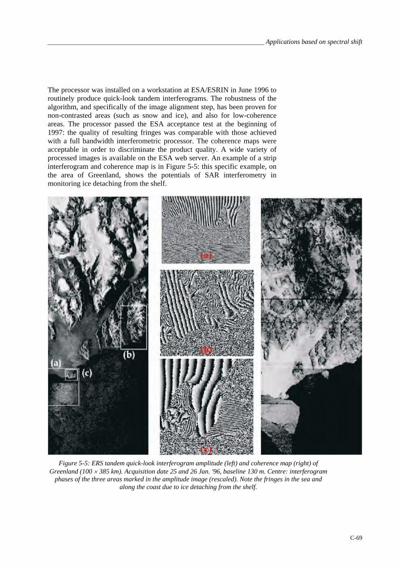
________________________________________________________________ Applications based on spectral shift
C-69
The processor was installed on a workstation at ESA/ESRIN in June 1996 to routinely produce quick-look tandem interferograms. The robustness of the algorithm, and specifically of the image alignment step, has been proven for non-contrasted areas (such as snow and ice), and also for low-coherence areas. The processor passed the ESA acceptance test at the beginning of 1997: the quality of resulting fringes was comparable with those achieved with a full bandwidth interferometric processor. The coherence maps were acceptable in order to discriminate the product quality. A wide variety of processed images is available on the ESA web server. An example of a strip interferogram and coherence map is in Figure 5-5: this specific example, on the area of Greenland, shows the potentials of SAR interferometry in monitoring ice detaching from the shelf.
Figure 5-5: ERS tandem quick-look interferogram amplitude (left) and coherence map (right) of
Greenland (100 × 385 km). Acquisition date 25 and 26 Jan. '96, baseline 130 m. Centre: interferogram phases of the three areas marked in the amplitude image (rescaled). Note the fringes in the sea and
along the coast due to ice detaching from the shelf.

TM-19 _________________________________________________________________________ InSAR Principles
C-70
5.3 Super-resolution The range super-resolution technique is based on the observation that, when the same target is imaged from different view angles, all the views can be combined to get an image at an enhanced resolution. This principle is the very root of Synthetic Aperture Radar, and is furthermore exploited in SAR-SPOT systems that steer the antenna azimuth pattern in order to pinpoint a fixed target.
The extension to the range case, suggested for the first time in [Prati92], results in range super-resolution. The basic principle is the one shown in Figure 5-3 (lower part) for two images, but it can be extended to a large number of images. The proper in-phase summation of all the images is slightly complicated by the fact that the image should be corrected for a constant phase shift and also properly calibrated in amplitude. Notice that the in-phase summation of overlapped spectral contributions may cause spectral modulation effects, and these are quite complicated to compensate for as the cross-correlation of each spectral component is not known a priori.
The final result would be a single super-resolution complex image. The actual resolution enhancement would depend upon the baseline span and the local topography.
One of the major limitations of the technique in repeat pass SAR interferometry is represented by the temporal decorrelation that would arise in the long time interval between acquisitions (> 35 days for ERS). In fact, in processing with ERS datasets, this technique provided its best results in presence of point scatterers, which are most likely to correlate over the long term. For this reason, very good results are expected by applying super-resolution enhancements in simultaneous or in very short revisit time SAR interferometry, like for the interferometric cart-wheel combination proposed by D. Massonnet (see for example [Massonnet01]), or for the ERS-Envisat tandem discussed in chapter C7.
One of the better examples of the capability of this technique is provided in [Suess98]: a resolution enhancement of a factor 2.7 was obtained by exploiting the technique described in [Prati93, Gatelli94] and coherently averaging 9 images (see Figure 5-6).

________________________________________________________________ Applications based on spectral shift
C-71
Figure 5-6: Super-resolution in urban areas: Harbour with oil storage, Amsterdam.
Left: incoherent average (9 images) Right: coherent average (range resolution enhancement of a factor 2.7). Range is horizontal in the images.
[Images courtesy of M. Suess, Daimler-Benz Aerospace Dornier]


_______________________________________________________________________ Differential interferometry
C-73
6. Differential interferometry
6.1 Introduction Distinguishing between ‘differential’ interferometry and ‘conventional’ interferometry is largely artificial, because interferometry is an intrinsically differential technique. Its ability to summarise all the geometric differences in range between two radar images is the result of several widely different phenomena. These phenomena can be regarded as different layers of information. Therefore, we must remove the various layers of geometric information one after another, in order to single out the one that is useful for a given application. As often in radar, the crucial word here is ambiguity. If there are n various causes of geometric difference involved in a final result (interferogram), one must know, in theory, the n – 1 first layers of information in order to acquire a good knowledge of the n th layer.
In the most general case, four different information layers are stacked in an interferogram. In other words, n = 4. Of these layers, two arise from the difference of point of view between the two images used to form the interferogram. These are the orbital residuals and the topographic residuals. Two additional layers come from the difference between the acquisition times of the pair of images. These are the displacements and the atmospheric artefact.
Specially designed systems allow a reduction of the number of layers. For instance, the Shuttle Radar Topography Mission (SRTM), flown for the first time in 2000, eliminated the time difference by acquiring the two images simultaneously. Thus it reduced the number of layers to two (topography and orbital residuals). Furthermore, since the two antennae were linked by a physical beam, the degrees of freedom of the orbital fringes were themselves severely reduced. This system was therefore well suited for topographic mapping.
The ideal situation in which all the contributors to the geometric changes except one are perfectly known almost never occurs. The n – 1 information layers will usually leave residuals that will create unwanted artefacts. These unwanted layers will also govern the strategy of image selection, as the user will seek to select scenes whose conditions of acquisition will amplify the useful information and minimise the rest. In the next section, we will recall the orders of magnitude of the various layers.
The most basic step in interferometry consists of subtracting the phases between two radar images in order to get rid of the randomness built within each pixel by the layout of elementary targets. But this step is only the beginning of a long series of subtractions, indicating that interferometry is differential by nature.
In this section, in order to better understand differential interferometry, we will assume the ideal situation in which we know every detail of the geometry of the site and of the orbits during each data take. We will then

TM-19 _________________________________________________________________________ InSAR Principles
C-74
explore the ways in which the actual situation drifts away from this ideal and how we can characterise these drifts and learn from them.
6.2 Differential interferometry using an available DEM
In principle, building differential interferometry software is straightforward if reliable external sources of information exist. For instance, if the shape of the landscape is correctly known from a digital elevation model (DEM), we can screen each point in the DEM, once properly sampled to meet the user’s needs, and define for each point the corresponding Cartesian vector P in a given reference system. Assuming we accurately know the orbits of the two satellite passes involved in the formation of an interferogram in the same reference system, we can determine the closest distance r to point vector P and the corresponding satellite position vector S and velocity vector V.
It is clear that the above knowledge comes either from conventional geometry (such as computing P for each point in the terrain grid), or from orbit propagation software (such as is required for determining r, S and V). We label the two radar images involved in the interferogram 1 and 2, using the convention that 1 refers to the oldest image, or, if the two are acquired simultaneously, to the one used as a geometric reference (i.e. the phase in 2 is subtracted from the phase in 1).
For each point of our ground sampling grid we can obtain P as well as S1, V1, r1 for the first image, and S2, V2, r2 for the second one. Writing software to do this can be simplified by reusing subroutines from geographic systems as well as from orbit computations. At the same time, we can easily define a unit vector U1 by:
1
1
rPS −
=1U Equation 6.1
We define a vector U2 similarly. These vectors point from the point of interest on the ground to the respective satellite’s positions at closest range.
If we now use the expression mod(r,2λ
) to mean the fractional part of r
expressed in units of half the wavelength λ , then the interferogram between images 1 and 2 should in principle exhibit the following phase value:
)),(),((2
rmod2
rmod421
λλλπφ −=Δ Equation 6.2
We can remove Δφ from the interferogram, thus turning it into a differential interferogram as it is depicted in Figure 6-1. This operation involves comparing very different numbers, for r amounts typically to 3 × 10⁷ times half the wavelength for ERS-1. However using double precision numbers or similar precautions can take care of the potential rounding problems in a software program.

_______________________________________________________________________ Differential interferometry
C-75
Figure 6-1: Drawing of ‘perfect world’ interferometry
Interferometry is a very straightforward technique. Assuming that the position of a satellite can be ascertained with arbitrary accuracy, so can the distance between it and any given point on the ground. We are then free to express this distance in units of wavelength. The expected ‘geometric phase’ can be computed for any point on the ground. However, this geometric phase cannot be extracted from a single image, where it is mixed with a seemingly arbitrary ‘construction phase’ which depends on the internal layout of elementary targets inside the pixel surface. Fortunately, if the interferometric conditions are met, the construction phase can be eliminated between two radar images, leaving the difference of the geometric phases. The difference of the geometric phases can also be simulated from the distances of the two satellite passes. The difference between the experimental phase difference and the simulated phase difference should leave a ‘flat’ interferogram as a result of a perfect knowledge of all the ground and orbital geometric features.
The sampling on the ground must obey two kinds of constraints: first, it is desirable to take advantage of the full content of information in the radar image. Therefore the ground sampling must be denser than the equivalent range and azimuth sampling of the radar, once it has been projected on the ground. Second, the signal represented by Δφ must be correctly sampled. In particular the change of Δφ from a point on the ground to any of its neighbours must stay below 2π. This is nothing more than the interferometric condition we have met before, in an earlier section (A.2.4).
For the sake of simplicity, we will assume that the generic differential processor consists, for each point on the ground, of the following four steps (this does not represent the most widely used procedure; however, an experimental processor [Massonnet00] implements it):
1. Selecting the position of the given point on the ground in range and time (i.e. across track and along track) in the two radar images to be combined,

TM-19 _________________________________________________________________________ InSAR Principles
C-76
2. Resampling the equivalent radar pixels in both images,
3. Subtracting the phases of these pixels and
4. Subtracting the geometric Δφ (the phase predicted by geometry).
The result of these steps is a map of the difference of phase in geographic coordinates, whose value should be zero if the assumptions for phase correction were fully accurate (i.e. the geometric prediction of the phase is exactly the observed phase difference between the images). In this case, the process would be useless because we would not have learnt anything from it!
The real world, however, is better represented by Figure 6-2, where all our initial assumptions are inaccurate to a certain extent.
Figure 6-2: Categorising interferometric content
In the real world, four causes make the prediction of Figure 6-1 wrong; two of these are related to the different viewing geometries of the two satellites:
1) Inaccuracy of orbit knowledge (for both satellites) 2) Inaccuracy of elevation knowledge
Two of the causes are related to the time elapsed between the data acquisitions:
3) The change in the radio-electric ‘depth’ of the atmosphere, itself linked to changes in pressure and moisture or to turbulence
4) Displacements of the ground taking place between the imaging sessions
One can therefore say that, with respect to the point of view, interferometry must obey a condition (the similarity of the point of view of both images) and provides two information layers (the accurate orbital positioning and the topographic residuals); whereas, with respect to the elapsed time, interferometry must obey another condition (the surface conservation) and provides two additional information layers (the atmospheric depth change and the ground displacements). All these ‘layers’ exist together in any interferogram, with different scales and sensitivities, unless a specific design cuts some of these. This is the case for the SRTM mission: having no time

_______________________________________________________________________ Differential interferometry
C-77
difference eliminates two layers, and the fixed-length beam reduces the degrees of freedom of the baseline (i.e. orbital) inaccuracy.
If our knowledge of the position of, say, the first satellite is wrong by δS1, this error causes a change of range of U1•δS1. The altitude of the point on the ground not being perfectly known also results in an error δP. We assume that only the vertical component, δh, of this δP is not zero. If we denote the vertical component of U1 ‘U1u’ (for ‘up’), the error in altitude creates a change in range of the first image:
δr1 = )1( 21uU
h−δ
Equation 6.3
The topographic error necessarily exists also in the second image, creating an almost identical change δr2 obtained by changing U1u to U2u in the expression. Apart from this shift in positioning, the error in altitude creates a round-trip phase change in the interferogram, due to the misalignment of the two wave-fronts, equal to (δr1 U1u – δr2 U2u) or, in phase:
Δφ = 4π )1()(
21
21
u
uu
UUUh
−−
λδ
Equation 6.4
We denote the change of elevation capable of creating a full 2π phase cycle between the images as the ‘altitude of ambiguity’. This is therefore equal to:
ha = )(2)1(
21
21
uu
u
UUU−
−λ Equation 6.5
It is clear that since the vectors U can be produced from procedures not related to any knowledge in the radar field, so can the altitude of ambiguity ha too. For changes in the two distances U1 and U2, it is only their difference that is accessible. This explains why interferometry is relatively insensitive to variations in topographic height. The angle (S1, P, S2) is so acute, constrained by the interferometric condition, that several tens or hundreds of metres are required to create a single topographic fringe, depending on the orbital separation. A good consequence of this, often surprising at first sight, is that a digital terrain model of only moderate accuracy is often sufficient to reduce the topographic content of an interferogram down to a negligible fraction of a phase cycle, thus leaving a ‘clean’ displacement map, accurate to millimetres.
The displacement in the terrain of point P occurring in the time elapsed between the acquisitions of the two images also creates a δP vector, which imposes changes only on the second image, creating a round-trip phase change in the interferogram equal to:
Δφ = – 4π λδPU •2
Equation 6.6
As a consequence, the line-of-sight component of any displacement of the terrain is directly recorded as a phase shift, and unlike topography, displacement in the millimetre range can be observed and measured.

TM-19 _________________________________________________________________________ InSAR Principles
C-78
Finally, the refractive index of the atmosphere, for the entire path traversed by the radar waves during the acquisition of either image, creates a contribution to the difference of phase. In a subsequent section we will distinguish between the effect of static atmosphere over flat terrain, the effect of static atmosphere over mountainous terrain, and the effect of heterogeneous troposphere or ionosphere on the signal. These effects introduce phase shifts that generally remain within one ERS fringe (equivalent to a terrain height displacement of 28 mm), but might occasionally reach several fringes.
In the above discussion, we have seen how the pointing vector U, a pure result of geographic and orbital knowledge, can be used to explain the behaviour of various geometric changes in an interferogram. The pointing vector also allows the definition of the limits of interferometric measurements to be examined. Let us define the ‘altitude of pixel’ hp as the elevation change that creates a change of range equal to the size of a range pixel. Q is the ratio of the carrier frequency and the range sampling frequency of the radar (Q is 279.5 for ERS), and the one-way range pixel
size is2λQ
, hence:
hp = uU
Q2
λ Equation 6.7
The altitude of pixel can be related to the altitude of ambiguity:
ha = ))2
(1()(
2
112
21
ppp
pp
hQ
hhQhh λ
−− Equation 6.8
Considering the change of altitude corresponding to the range pixel of image 1, in the presence of a displacement gradient creating δP between each range pixel, and with a slope creating δh between each range pixel, the global condition for which interferometry is feasible is:
12 2 <•
−+λ
δδ PUhh
hh
aa
p Equation 6.9
It is theoretically possible that a pair of images outside this interferometric
domain (for instance because 1>a
p
hh
) could nonetheless produce a local
interferogram because of a local displacement gradient that counteracts the first term. Alternatively, a strong deformation gradient may push an interferogram outside the interferometric domain, even if the satellite orbital baseline separation is small. This may happen in the vicinity of terrain faults or in glaciers.

_______________________________________________________________________ Differential interferometry
C-79
6.3 Differential interferometry with three or more combined images
A ‘radar only’ approach to producing differential interferograms without using any external information is very appealing. It requires at least three radar images.
Figure 6-3 shows the assumed geometry of a landscape captured by any two radar images, labelled Master and Slave. The third image (and any additional images) would be similar to the Slave, but is not shown in order to simplify the drawing.
Figure 6-3: Description of interferometric geometry
In the master image, from the near-range to the i th pixel, the distance changes from R0 to R0+iΔ , Δ being the range pixel size. In the slave image, the point observed at near-range by the master is actually offset by p pixels (p can be positive or negative, and is generally not an integer, unlike i). In the current point with altitude hi, the range to the slave track equals the one of the master, plus the near range offset, plus the number of fringes counted from the near-range to point i . The fringe count must be divided by the factor Q to be expressed in units of range pixels. The distance between the tracks is d , angles θ and gi, used in the development, complete the geometric description. Of course, in reality the Earth is not flat, but taking a ‘flat’ reference (for instance given by the plane tangential to the surface at mid-swath) is more convenient and does not affect the principles underlying the following discussion. As usual, we choose one of the images arbitrarily as a geometric reference (the master image). The others will be called, respectively, the slave image and the complementary image. Their values are denoted by m , s
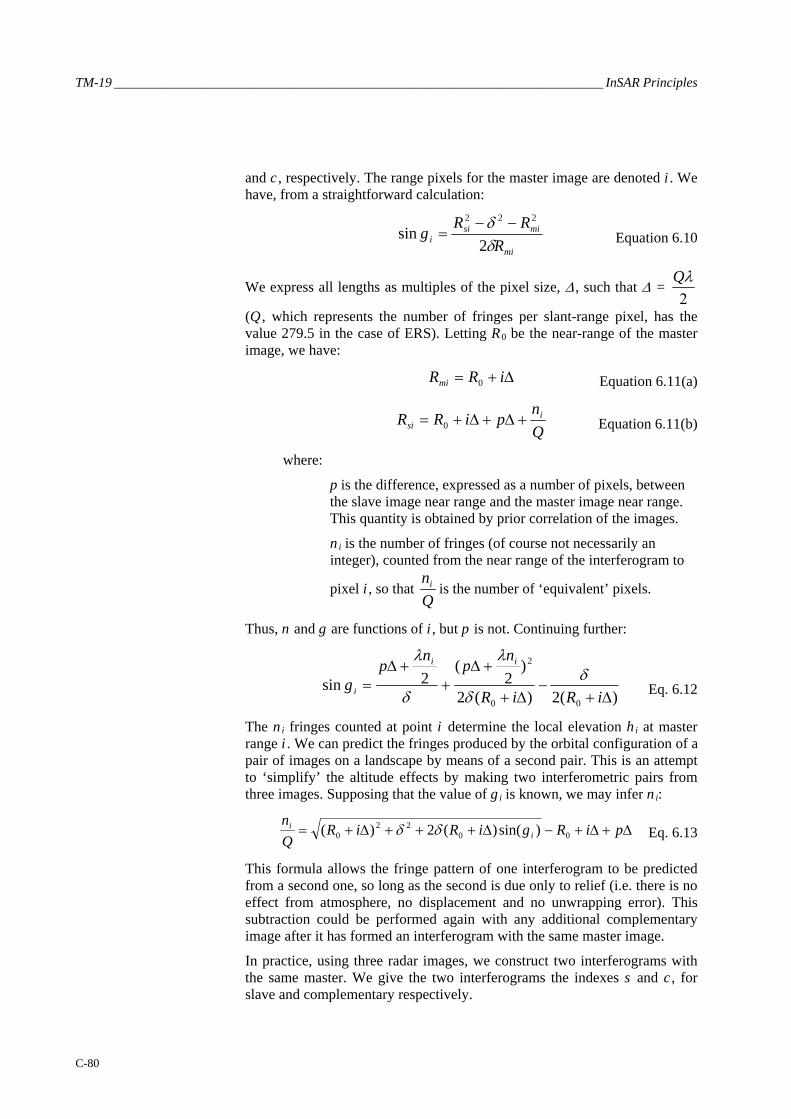
TM-19 _________________________________________________________________________ InSAR Principles
C-80
and c , respectively. The range pixels for the master image are denoted i . We have, from a straightforward calculation:
mi
misii R
RRg
δδ
2sin
222 −−= Equation 6.10
We express all lengths as multiples of the pixel size, Δ , such that Δ = 2λQ
(Q , which represents the number of fringes per slant-range pixel, has the value 279.5 in the case of ERS). Letting R0 be the near-range of the master image, we have:
Δ+= iRRmi 0 Equation 6.11(a)
Qn
piRR isi +Δ+Δ+= 0 Equation 6.11(b)
where:
p is the difference, expressed as a number of pixels, between the slave image near range and the master image near range. This quantity is obtained by prior correlation of the images.
n i is the number of fringes (of course not necessarily an integer), counted from the near range of the interferogram to
pixel i , so that Qni is the number of ‘equivalent’ pixels.
Thus, n and g are functions of i , but p is not. Continuing further:
)(2)(2
)2
(2sin
00
2
Δ+−
Δ+
+Δ+
+Δ=
iRiR
np
np
gii
iδ
δ
λ
δ
λ
Eq. 6.12
The ni fringes counted at point i determine the local elevation hi at master range i . We can predict the fringes produced by the orbital configuration of a pair of images on a landscape by means of a second pair. This is an attempt to ‘simplify’ the altitude effects by making two interferometric pairs from three images. Supposing that the value of gi is known, we may infer ni:
Δ+Δ+−Δ+++Δ+= piRgiRiRQn
ii
0022
0 )sin()(2)( δδ Eq. 6.13
This formula allows the fringe pattern of one interferogram to be predicted from a second one, so long as the second is due only to relief (i.e. there is no effect from atmosphere, no displacement and no unwrapping error). This subtraction could be performed again with any additional complementary image after it has formed an interferogram with the same master image.
In practice, using three radar images, we construct two interferograms with the same master. We give the two interferograms the indexes s and c , for slave and complementary respectively.

_______________________________________________________________________ Differential interferometry
C-81
First, we calculate gs(i) from ps, ns(i) and ds, which are the values for the first interferogram (master-slave).
Next, we define the look angle gs(i) – θ s, which is equal to gc(i) – θ c because the master radar beam direction is common to the two interferograms. In practice, only the difference θ c – θ s is needed for this operation. Finally, we recalculate sin(gc) by means of δ c and pc to calculate
Qinc )(
, from which nc(i) follows.
We may subtract these calculated fringes from the second interferogram, leaving only the phase shifts due to changes on the ground. The second interferogram does not need to be unwrapped at this stage. The advantage of the method is that it does not require external data other than radar images. The first drawback of the method is that it assumes the geometric differences between master and slave to be due only to topography, which is usually wrong to some extent due to atmospheric artefacts.
Another drawback is the difficulty in deciding whether movements in the terrain have occurred in the master-slave image pair or the master-complement pair. Both can influence the final result. This drawback is shared by the integer combination technique (see below).
Finally, it is necessary to resolve the phase ambiguity (see section “phase unwrapping”) prior to the application of the technique.
6.4 Techniques to avoid phase unwrapping
6.4.1 Integer combination The ambiguous nature of the fringes within a wrapped interferogram make it of limited practical value. In particular, no linear combination nor any kind of scaling can be undertaken on a ‘wrapped’ interferogram. Despite the improvements of various methods for phase unwrapping, an active field of research that goes beyond radar imagery, unwrapping is still difficult, risky and damaging. It is risky because of the possible introduction of errors that will be incorporated in any further processing steps and which will become impossible to recognise easily after any scaling of the resulting interferogram. It might also be damaging because the software will be forced to black out parts of the image where the coherence is too low. The areas that cannot be unwrapped have poor coherence, but often contain some information that will be lost by this thresholding process. After correction for topographic and orbital contributions, the interferogram contains three kinds of information:
1. The fluctuation in the number of fringes due to the noise ν , either from thermal noise or partial incoherence of the terrain in the time elapsed
2. The number of fringes ah
εdue to the errors ε in the DEM, where ha is
the altitude of ambiguity.

TM-19 _________________________________________________________________________ InSAR Principles
C-82
3. The number of fringes μ caused by any differential effects, including local variations in the atmospheric thickness, as well as local ground motion between the data takes.
All three quantities (ν , ε and μ) vary greatly across the image. In contrast, ha is rather stable, usually varying gently with range and not at all with azimuth.
The interferogram in which the effects of topography and the ‘orbital fringes’ have been retrieved gives us the fractional part of:
ah
εμν ++ Equation 6.14
It cannot be mathematically manipulated by the formulas of the double difference unless it has been unwrapped. However, we can manipulate the interferogram while preserving its integer and fractional parts. If we multiply the interferogram by an integer q1, we will likewise multiply the number of phase transitions and the initial integer values. Note that the integer values remain unknown unless unwrapping has been performed. We obtain the fractional part of:
ae
qqq εμν 1
11 ++ Equation 6.15
If we combine the first interferogram with a second, characterised by another independent noise distribution, another altitude of ambiguity, other differential effects and another multiplication factor q2, but the same local DEM error ε , we obtain the fractional part of:
( ) ( ) ⎟⎟⎠
⎞⎜⎜⎝
⎛+++++
2
2
1
122112211
aa hq
hq
qqqq εμμνν Equation 6.16
where the quantities related to the first and second interferograms are indexed by 1 and 2 respectively.
As a consequence of the multiplications, the RMS amplitude of the noise becomes:
22
22
21
21 nqnq + Equation 6.17
This resulting increase of the noise in practice limits the choice of the absolute value of q1 or q2 to less than 3. Otherwise, once multiplied by a
typical factor of 22
21 qq + , the noise distribution could too easily exceed
one cycle, and the result would be useless. Noise is usually responsible for a phase uncertainty equivalent to a few percent of a cycle.
The interferogram resulting from this kind of combination exhibits an equivalent altitude of ambiguity hae, written as:
2
2
1
11
aaae hq
hq
h+= Equation 6.18

_______________________________________________________________________ Differential interferometry
C-83
The consequences of the above formula are easy to understand. Phase unwrapping is only required for altitudes of ambiguity lower than the typical accuracy of globally available Digital Elevation Models and higher than the ones set by the interferometric limit. Formerly this ranged from 200 m (the accuracy of GLOBE dataset) to 10 m (the interferometric limit of ERS). Now the altitudes of ambiguities for which unwrapping might be required range from 30 m (accuracy of the publicly available global DEM produced by the Shuttle Radar Topography Mission) to a few metres. As a consequence, even if the choice of q1 and q2 is limited to ±1, ±2 or ±3, there will be combinations which can emulate equivalent altitudes of ambiguity larger than 30 m most of the time. Even if the resulting interferograms are generated in a map-projected geometry, which means independently of the radar image geometry, it is possible to use the technique between pairs from ascending and descending orbits or between pairs from different satellites.
The technique of integer combination often contradicts intuitive expectations about fringe behaviour. After modelling the dense fringe pattern (Figure 6-4(a)) with a horizontal fringe pattern of the same density (Figure 6-4 (b)), we subtract the horizontal fringe model from the initial fringe pattern and obtain, surprisingly, a purely vertical pattern (Figure 6-4 (c)).
Figure 6-4: Illustration of interferometric combination. Set of fringes (a to c) that
contradicts ‘natural’ opinion about fringe behaviour.
Similarly, even ambiguous (i.e. ‘wrapped’) interferograms can be manipulated by linear combination provided they are multiplied by whole numbers. In an ambiguous interferogram, we can basically ignore the integer part of the fringes. This part remains an integer only if it is multiplied by an integer. We simulate an interferogram on Mount Etna with a topographic sensitivity of 130 m per fringe (Figure 6-5(d)). We then simulate another interferogram with a sensitivity of –255 m per fringe (Figure 6-5(e)). Multiplying the first interferogram by two (which doubles the number of fringes) and adding the result to the first interferogram creates a new interferogram with a topographic dependence decreased to –6630 m per fringe (Figure 6-5(f)).

TM-19 _________________________________________________________________________ InSAR Principles
C-84
Figure 6-5: Illustration of interferometric combination (d to f). In d), we have a
simulated mountain with a topographic sensitivity of 130 metre-per-fringe. In e), we have a sensitivity of –255 metre-per-fringe. Simply adding twice e) to d) provides an image of the simulated mountain featuring a topographic dependence decreased to
–6630 metre-per-fringe seen in f).
In this last image, unwrapping becomes unnecessary because the mountain is not as high as the elevation represented by a single fringe. The combined interferogram (Figure 6-5(f)) can therefore be multiplied by a non-integer coefficient in order to automatically unwrap the image of (Figure 6-5(d)) (the most sensitive to topography) and to obtain an accurate elevation map.
6.4.2 Interferogram stacking Another useful idea to bypass, at least partially, the need for phase unwrapping is interferometric stacking [Sandwell98]. According to this procedure, each interferogram of a series is first derived (i.e. the gradients of the phase are computed). The phase gradients are not ambiguous and can be scaled according to the orbital separation in order to reach a normalised topographic sensitivity. After being scaled, the gradients of the series are stacked and averaged. At this stage, this or that contributor (for instance the topographic contribution) to the interferometric information can be removed using a priori knowledge. During this operation, one may reasonably hope that atmospheric residuals are efficiently attenuated and that their averaged gradient is close to zero. The average interferogram is then reconstructed by integration. Global, FFT-based reconstruction methods are especially efficient for unwrapping gradients with values close to zero. Similarly to the integer combination method, the method can be used not only to cancel out topography, but also to eliminate deformation gradient proportional to time, by proper scaling, or any other specific contributor.
The drawback of the method is the difficulty in computing gradients on noisy phase images, which requires delicate pre-filtering. Sandwell et al. describe the necessary precautions to be taken.

_______________________________________________________________________ Differential interferometry
C-85
6.5 Information contained in interferometric measurements
6.5.1 Residual orbital fringes Usually the first term to be corrected right after the production of an interferogram corresponds to residual orbital fringes. These fringes are generally the dominant signal in the raw differential interferogram, and even a very good assessment of orbital position can lead to a significant number of residual fringes. Using the notations of previous sections, an error δS on the satellite’s position creates a number of fringes f amounting to:
f = 2 λδSU •
Equation 6.19
Let us assume that we can assess the number of residual fringes, both at near range f n and at far range f f, together with the corresponding pointing vectors Un and Uf, themselves almost insensitive to the changes caused by δS . Since Un and Uf are not collinear, we may assume:
δS = αUn + βUf Equation 6.20
which leads to:
λ f n = 2α + 2βUf•Un Equation 6.21 (a)
λ f f = 2αUn•Uf + 2β Equation 6.21(b)
The system yields α and β and finally δS . A first problem is that we do not know f n and f f but only their difference f f – f n. A quick fix would be to assume f n = 0, but what are the consequences? To answer the question, let us assume that δS results from f n = 0 and f f = f and that δS ' results from f n = n and f f = f + n . By definition, δS and δS ' are equally valid at far range and near range. Let us assume an intermediate range where the pointing vector is written:
U = x Un + y Uf Equation 6.22
with the unit condition:
U2 = x2+y2+2xyUf•Un = 1 Equation 6.23
The difference in correction for U depends on whether it is computed from δS or δS ':
( )fyxSSSS UUU n +•−=•− )'(2
)'(2
δδλδδλ Equation 6.24
Using the relations:
0)(2
=• nUSδλ; fUS f =• )(
2δλ
;
nUS n =• )'(2
δλ; nfUS f +=• )'(
2δλ
Equation 6.25

TM-19 _________________________________________________________________________ InSAR Principles
C-86
we have:
)'(2
SS δδλ− •U = yf – xn – y (f+n) = –n (x+y) Equation 6.26
We assumed a shift of n fringes between the two corrections. The unexpected difference between the corrections, which we later call the ‘error’, is therefore: n (1 – x – y) fringes. Let us now observe that Uf•Un is the cosine of the antenna aperture of the radar in elevation (pointing difference between near range and far range). If W is the useful height of the antenna, that is about one metre for ERS, we have:
2
2
21
Wnfλ
−≈• UU Equation 6.27
hence:
( ) 2
22 1
Wxyyx λ
+≈+ Equation 6.28(a)
2
2
21
Wxyyx λ
+≈+ Equation 6.28(b)
leading to an error of magnitude: 2
2
2Wxyn λ
, x + y being close to one. The
maximum is obtained for x = y = 0.5, that is for the intermediate point
between far and near range. The worst case error becomes: 2
2
8Wnλ
; we want
this ‘error’ to remain a small fraction of the wavelength. We choose for
instance: 2
2
8Wnλ
< 32λ
Finally, we observe that n fringes is the error made on the estimation of the range of the second image when it corresponds to the near-range of the first image. The absolute number of fringes has no importance as long as it is
such that: n < λ4
2W
For ERS-1, n fringes must be smaller than 4.5 m to obey the above condition. Since the interferometric processing requires the two images to be superposable to better than a fraction of the range (or azimuth pixel), we may consider that it is always met (ERS range pixel size is 7.9 m).
A second problem is that we do not know which orbit to move, that is, how the error is distributed between the orbits. In order to know more about this, we will use the following trick: we take two widely separated ERS orbits in order to be in a ‘worst case’ situation. We then generate a fake interferogram: a constant image filled with zeroes. We then use an ‘orbital tuning’ program to correct the fake interferogram by a number of residual fringes typical of the accurate assessment of ERS’s orbital paths. We correct the interferogram with a typical ‘orbital’ fringe pattern, amounting to zero,

_______________________________________________________________________ Differential interferometry
C-87
eleven, six and a half and fifteen fringes at each corner. As a consequence, our interferogram, initially ‘flat’, exhibits this number of fringes (shown in Figure 6-6(a)). We ask the program to execute this first correction by moving only the first orbit.
Figure 6-6: Illustration of the error in orbital tuning
Next, we run the program again in order to eliminate the fringes we just created, but we ask the program to correct only the second orbit. This time, we correct the four corners of the interferogram by the opposite quantities, respectively, by zero, minus eleven, minus six and a half and minus fifteen fringes. The result (Figure 6-6(b)) is flat to within the maximum error that can be committed by a wrong sharing of the responsibility between orbits. The figure clearly shows that this error is not a matter of concern (typically one grey level). Such a conclusion would not apply if the initial orbital error could have produced tens of residual fringes.
Orbital tuning provides a unique solution if one of the trajectories can be said to take all the error for itself. In reality of course both trajectories are faulty to some extent. What is the residual error we commit in correcting one trajectory for the full error? To assess this we take two orbits close to the maximum orbital separation permitted by the principles of interferometry, then we ‘correct’ an initially flat interferogram, introducing a number of fringes by moving one of the orbits (part a). We then correct the fringes, considered as an artefact, by modifying the second orbit. The result (part b) is representative of the maximum error that could be made using the ‘single orbit hypothesis’. In order to make the result visible, the error image (b) has been multiplied by 256, so that the maximum error (the white surfaces) corresponds to 1/256 cycle, well below any reasonable accuracy threshold of SAR interferometry. The structure of the error is mainly governed by the

TM-19 _________________________________________________________________________ InSAR Principles
C-88
topography of the area. A high relief area has been selected in this test, run by H. Vadon of CNESiii.
6.5.2 Uncorrected topography Some topographic residuals arise from uncorrected topography or errors in the DEM used. The errors are scaled by the topographic sensitivities of the pairs involved, which is the basis of the pair-wise logic that can be used to discriminate these effects from others.
6.5.3 Heterogeneous troposphere The contribution of heterogeneous atmosphere was first detected in 1994 [Massonnet94], and quickly confirmed as the major limitation of interferometric accuracy for displacement mapping as well as for topographic reconstruction. The signature of this artefact is linked to the date of the data takes. A given image will propagate the structures created by various delays through clouds, pressure waves, etc. in any interferogram in which the image is a part constituent. The structure would always have the same amplitude, although its sign would change depending on whether the faulty image is used as master or slave in the combination. This behaviour allows an easy screening of atmospheric effects if several interferograms are available on a given site.
Figure 6-7 shows the effect of cloud ‘rolls’ in eastern United States. To the experienced eye, the atmospheric effects can be recognised directly (i.e. even if a single interferogram is available), because they have typical shapes and ‘ragged’ borders that are not usually found in topographic or displacement signals. Figure 6-7 is an example of visualisation of meteorological phenomena through radar interferometry. These phenomena are characterised by their insensitivity to the time elapsed between the acquisition of the images used to form the interferogram, as well as their insensitivity to the orbital separation of the corresponding satellite tracks. However, a given radar image is responsible for the same structure observed in several interferograms with a constant magnitude.
iii By personal communication

_______________________________________________________________________ Differential interferometry
C-89
Figure 6-7: Atmospheric heterogeneity, cloud ‘rolls’ in eastern US. Here we see the
effect of atmospheric turbulence generated by winds interacting with topography. The topographic contribution from the Blue Mountains, east of Washington, has not
been corrected. The 1000 m or so high mountains can hardly create one fringe in this interferogram that is not very sensitive to topography. However, the wind
‘rolls’ as it crosses the topography, creating waves that are easy to see in dark blue. Their amplitude is very low – 3 mm crest to crest – but their structure makes them
easy to spot. The images were separated by 3 days.
6.5.4 Heterogeneous ionosphere The ionosphere is likely to alter the signal in a similar manner to the troposphere [Massonnet94], except that the ionosphere is a much thicker layer than the troposphere and actually extends up to the satellite’s orbit. As a consequence, it is more difficult to relate external data (such as GPS paths) to an artefact. However, the heterogeneity of the ionosphere is less than that of the troposphere and is not influenced by the topography. Similarly, the ‘static ionosphere’ does not create artefacts, because it is above any topography. The way to discriminate the effect of the ionosphere is the same as for detecting a heterogeneous troposphere.

TM-19 _________________________________________________________________________ InSAR Principles
C-90
6.5.5 Static atmosphere Since the refractive index of the atmosphere is not exactly equal to one, all rays emitted by a radar undergo a curvature which results in a consistent apparent displacement of the satellite [Tarayre96]. However, if some topography is present in the scene, the depth of atmosphere effectively crossed by the wave varies. If the general features of the atmosphere (e.g. the moisture density) change between the two data takes used to form an interferogram, a difference in delay will appear, modulated by the topography. The signature of this effect is an interferogram in which structures linked to topography appear, but without any relationship to the orbital separation of the pair. This ‘topography’ would be seen even without any orbital separation.
6.5.6 Radar clock drift In the course of interferometric experiments with ERS-1 over very long data strips, some parallel fringes were found to remain even after orbital fringes had been removed. Although it is difficult to prove firmly the origin and nature of these remaining fringes, a possible explanation is that this is due to a frequency drift of the local oscillator onboard the radar [Massonnet95B].
We assume the carrier frequency is:
f c = f0 + t fb Equation 6.29
where f b is a time-dependent bias of the ‘official’ frequency f0 (5.3 GHz for ERS, used in the experiment). The bias can create ‘clock fringes’ if the carrier frequency has drifted somewhat when the pulse returns. It is then mixed with a slightly different frequency, typically after a number k of inter-pulse periods (k equals 9 for ERS). If f a is the pulse repetition frequency, the fringe rate, expressed in fringes per second, is:
a
b
fkf
Equation 6.30
If data from ERS-1 and ERS-2 are mixed in an interferogram, only the difference of their frequency biases will contribute to clock fringes. A difference in their f0 would be cancelled when remixed. So there is no real difference between mixing ERS-1 with ERS-2 or working with the same satellite. In either case, the fringe rate would be:
a
bb
fffk )( 21 −
Equation 6.31
Several attempts to find more examples of the ‘clock artefact’, in particular for ERS-2, failed. The only example remains the one which was obtained by combining two very long data strips (about 2000 km) over eastern Europe (Figure 6-8). The data were acquired on 25 September and 1 October 1991 and showed very little sensitivity to topography.

_______________________________________________________________________ Differential interferometry
C-91
Figure 6-8: Processing a long strip of ERS-1 data from Ukraine to Finland that
exhibits a series of fringes that cannot be explained by topography (the whole area is rather flat), displacement, or by atmospheric changes (the amplitude is too large)
The stability of the clock for ERS-1 was designed to be good over about one second, but by good fortune it was found to perform well in practice over a period of five minutes, very much better than specified. This allowed the radar to produce long segments of interferometric data without ‘interfering with itself’ too much. To allow this to be done again in future, a much higher clock stability should be planned at the design phase and preferably made a requirement.


______________________________________________ Envisat-ASAR interferometric techniques and applications
C-93
7. Envisat-ASAR interferometric techniques and applications In this chapter we will extend the interferometric techniques and applications discussed so far to the case when two acquisitions are made from different SAR modes, for example ScanSAR and Alternating Polarisation mode, and combined interferometrically. Such combinations have achieved progressively more importance since the first ScanSAR sensors (SIR-C, SRTM, RADARSAT) demonstrated the capabilities of ScanSAR interferometry.
7.1 Introduction We will focus here mainly on the Envisat-ASAR sensor, which has three acquisition modes that can be combined interferometrically:
• The conventional full resolution SAR mode, named Image Mode (IM) • An Alternating Polarisation Mode with multi-polarity capabilities (APM) • A ScanSAR mode with Wide Swath coverage (WSM)
The geometry of these acquisition modes is sketched in Figure 7-1, and the main features have been summarised in Table 7-1.
Figure 7-1: Interferometric modes of Envisat ASAR
Mode Swath Coverage (km)
Space resolution
Polarisations
IM IS1–IS7 14o–45o
50–100 30 m VV or HH
AP IS1–IS7 14o–45o
50–100 30 m VV+HH; VV+HV; HH+HV
WSM SS1–SS5 16o–44o
400 150 m VV or HH
Table 7-1: Envisat acquisition modes

TM-19 _________________________________________________________________________ InSAR Principles
C-94
Both AP and WSM are ScanSAR modes: the capability of performing interferometry in such modes will be discussed in the next section. We will generalise the interferogram generation technique, discussed in chapter 2 for the combination of two full resolution SAR images, to the combination of two images taken with different modes and resolution. Thereafter, we will detail the possible interferometric combinations of Envisat ASAR, and present some applications.
7.2 ScanSAR: an introduction ScanSAR is Synthetic Aperture Radar with swath coverage, in slant range, that is wider than that of conventional SAR systems. This coverage is achieved by scanning different sub-swaths, i.e. by switching the antenna look angle into different positions [Moore81, Currie92].
The geometry of a five sub-swath ScanSAR (e.g. Envisat’s ASAR WSM) is shown in Figure 7-2. The ScanSAR sensor acquires short ‘bursts’ of radar echoes for a time interval TD (dwell time) by cyclically scanning all the Ns sub-swaths.
Figure 7-2: Geometry of the five beams (or sub-swaths) of ScanSAR
This specific acquisition scheme allows for the coverage of a ground scene that is Ns times wider than that of a conventional SAR mode (∼400 km for Envisat and RADARSAT), at the same SNR balance (the transmitted power is always concentrated in one beam only), but with a proportional loss in the azimuth resolution [Currie92].
An undesired effect of the burst mode acquisition is a non-stationary Doppler history. This fact is evident in Figure 7-3: when an acquisition is being made, each target in the footprint is imaged from a different angle (three targets are represented here). Hence, both the amplitude and the phase

______________________________________________ Envisat-ASAR interferometric techniques and applications
C-95
of an echo depend upon the displacement between the target and the burst. In particular, the target located at the centre of the antenna beam when the acquisition is on provides the strongest contribution and its spectrum will be centred on the Doppler centroid, fDC.
Figure 7-3: ScanSAR acquisition of three different targets. The Doppler phase
history and the amplitude are differently weighted depending on the azimuth time of the target with respect to the scan pattern.
The resulting azimuth-variant amplitude is known as scalloping. Scalloping is the major drawback of ScanSAR, when fine amplitude calibration is required, as it introduces an azimuth variant CNR (Clutter to Noise Ratio). The sole possibility for reducing scalloping is to have the same target imaged in several looks or bursts, Nb, from different viewing angles. In ASAR WSM, for example, three azimuth ‘looks’ have been acquired (i.e. Nb = 3) for each target. The dwell time is then limited to TD < TF /(NsNb), NsNb being the product of looks × sub-swaths. This in turn worsens the geometric resolution, giving 150 m for the ASAR WSM. However, the radiometric accuracy is improved.
7.2.1 Acquisition The impact of the burst acquisition of the focused ScanSAR data can be easily understood in the 1-D case (quite reasonable, as ScanSAR has a large resolution cell). We start from the SAR acquisition, in a simplified, straight geometry (see for example [Bamler92]):
( ) ( )( ) ( )( )20 πexp/, ξθξξ −+−= tfjrtvaths Rs Equation 7.1
where hs(t)is the signal incident on a point scatterer ξ is azimuth time

TM-19 _________________________________________________________________________ InSAR Principles
C-96
ro is the slant range a( ) represents the antenna gain, as a function of the angle β(t) = –v(t–ξ)/r0, fR is the Doppler rate θ s the squint angle
The notation hs(t ,ξ) has been introduced to distinguish the signal domain, t , from the data domain, ξ . However, the SAR acquisition is stationary (azimuth invariant) as hs actually depends upon the difference (t – ξ). But when we apply the burst window, rect(t /TD), the azimuth invariance is lost:
hs(t ,ξ) = a(v(t– ξ)/r0+θ s) exp(jπfR(t– ξ)2 ) rect(t /TD)
–TF/2 < t < TF/2 Equation 7.2
This is made clear in Figure 7-3, which shows in the upper-left corner the contributions of the three echoes that add up to the burst.
The effect of the burst on the spectrum of the acquired echo can be simply evaluated by transforming (Equation 7.2). We need to apply the Method of Stationary Phaseiv (MSP) (see, for example, [Curlander91]).
2||
,rect)2(expexp),(2
PRFff
Tffff
fjf
fjffafH
DC
DR
DCR
RRs
<+
⎟⎟⎠
⎞⎜⎜⎝
⎛ ++−⎟⎟
⎠
⎞⎜⎜⎝
⎛−⎟⎟
⎠
⎞⎜⎜⎝
⎛≅
ξπξ
πξ β Eq. 7.3
where fDC = –2v /c f0sin(θ s) is the Doppler centroid.
Here again we have indicated the dependence of the spectrum of each echo on the actual location of the scatterer: Hs(f ,ξ ). The burst mode acquisition accounts for the last term in Equation 7.3. The effect is twofold:
• the spectrum of each echo has a reduced bandwidth Bs = fRTD, hence also a coarse resolution;
• the spectrum is bandpass, and its central frequency depends on the target location:
f c = fDC + fRξ Equation 7.4
7.2.2 Focusing Focusing, in ScanSAR systems, means assigning to each target in the whole (large) footprint the proper contribution to the (short) burst. The simplest way to get phase-preserving ScanSAR focusing is to apply the same SAR reference, i.e., matched to (Equation 7.1), to the burst, after zero-padding it for the duration of the footprint. We assume here to compensate for the azimuth antenna pattern by the proper inverse referencev, we get:
iv We assume here that the azimuth time-bandwidth product (in the burst duration)
is much greater than one. For very low resolution ScanSAR, different focusing schemes should be implemented, see reference [MontiGuarnieri2001].
v In SAR processing, the antenna pattern compensation is not usually performed. In ScanSAR this is required if scalloping compensation is needed on the basis of a single burst, see also [Bamler95B].
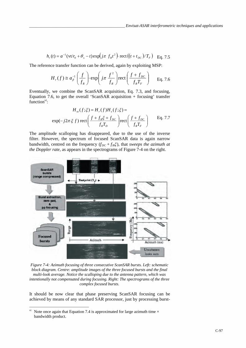
______________________________________________ Envisat-ASAR interferometric techniques and applications
C-97
( ) ( )( )FDCRsr Ttttfjtrath /rect exp)vt()( 21 +⋅−+/= 0− πθ Eq. 7.5
The reference transfer function can be derived, again by exploiting MSP:
⎟⎟⎠
⎞⎜⎜⎝
⎛ +⎟⎟⎠
⎞⎜⎜⎝
⎛⋅⎟⎟
⎠
⎞⎜⎜⎝
⎛≅ −
FR
DC
RRr Tf
ffffj
ffafH rectexp)(
21 πβ Eq. 7.6
Eventually, we combine the ScanSAR acquisition, Eq. 7.3, and focusing, Equation 7.6, to get the overall ‘ScanSAR acquisition + focusing’ transfer functionvi:
⎟⎟⎠
⎞⎜⎜⎝
⎛ +⎟⎟⎠
⎞⎜⎜⎝
⎛ ++−
==
FR
DC
DR
DCR
srss
Tfff
Tffff
fj
fHfHfH
rect rect )2exp(
);()();(
ξξπ
ξξ
Eq. 7.7
The amplitude scalloping has disappeared, due to the use of the inverse filter. However, the spectrum of focused ScanSAR data is again narrow bandwidth, centred on the frequency (fDC + fRξ), that sweeps the azimuth at the Doppler rate, as appears in the spectrograms of Figure 7-4 on the right.
Figure 7-4: Azimuth focusing of three consecutive ScanSAR bursts. Left: schematic block diagram. Centre: amplitude images of the three focused bursts and the final multi-look average. Notice the scalloping due to the antenna pattern, which was
intentionally not compensated during focusing. Right: The spectrograms of the three complex focused bursts.
It should be now clear that phase preserving ScanSAR focusing can be achieved by means of any standard SAR processor, just by processing burst-
vi Note once again that Equation 7.4 is approximated for large azimuth time ×
bandwidth product.

TM-19 _________________________________________________________________________ InSAR Principles
C-98
by-burst, and by (previously) zero-padding each burst to the duration of the whole footprint.
If the desired output is a multi-look image, it would be sufficient to detect and average all the focused bursts (in practice, only Nb bursts contribute at each azimuth), as shown in Figure 7-4.
The use of conventional SAR focusing to perform ScanSAR focusing is however not efficient at all, as the output image will be sampled at the SAR PRF rate, that is many times the Shannon limit (the inverse of the resolution). For example, in ASAR WSM, the ScanSAR resolution is 30 times coarser than the IM one.
To this end, several algorithms have been proposed in the literature for computing ScanSAR phase-preserving focused images directly at the low sampling rate: see [Bamler96, MontiGuarnieri96A, Moreira96, Cumming97, Lanari98]. These algorithms are different implementations of the same transfer function, with comparable computational efficiency.
7.3 ScanSAR interferometry Let us suppose we have two (repeat-pass) ScanSAR acquisitions, by perfectly synchronised scans, parallel orbits and the same Doppler Centroid.
The generation of a multi-look ScanSAR-ScanSAR interferogram can be achieved by separately processing each burst [MontiGuarnieri96A]. First, phase-preserving focusing should be performed (see section C.6.2.). Next, all the steps described in chapter B2 for normal SAR interferometry should be applied, with the exception of the common band filtering (not required for synchronised acquisitions):
1) range oversampling 2) spectral shift filtering 3) slave co-registration 4) Hermitian multiplication
The interferograms achieved by processing different bursts should be coherently averaged: the mosaicking is similar to that shown for the amplitudes in Figure 7-6. A slightly different approach is found in [Bamler99].
In the actual implementation, one should ensure that the data were focused with the correct Doppler rate, and that the co-registering parameters are quite accurate (better than the ScanSAR resolution!). It can be shown that very small errors in these parameters will introduce phase artefacts and bias. A technique to provide the proper estimate of co-registering parameters for ScanSAR is described in [Moreira00].
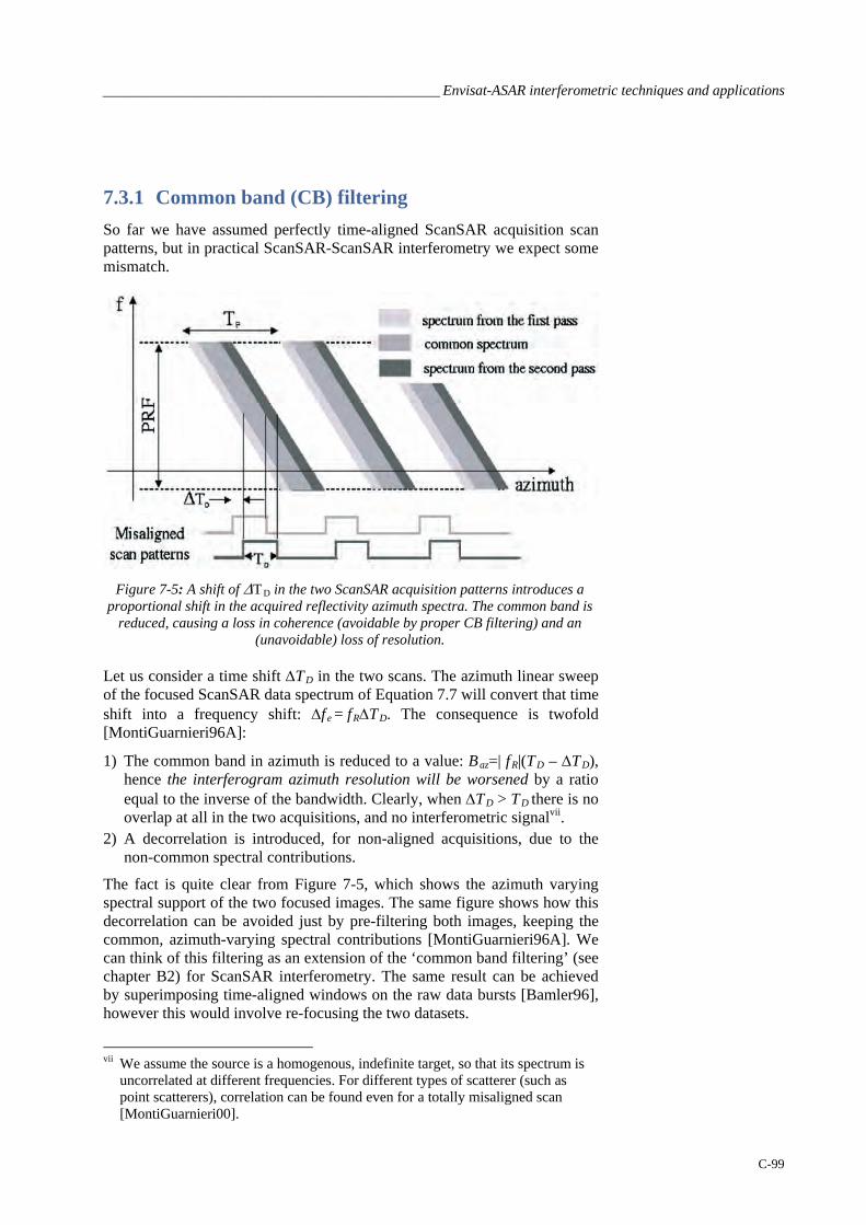
______________________________________________ Envisat-ASAR interferometric techniques and applications
C-99
7.3.1 Common band (CB) filtering So far we have assumed perfectly time-aligned ScanSAR acquisition scan patterns, but in practical ScanSAR-ScanSAR interferometry we expect some mismatch.
Figure 7-5: A shift of ΔTD in the two ScanSAR acquisition patterns introduces a proportional shift in the acquired reflectivity azimuth spectra. The common band is
reduced, causing a loss in coherence (avoidable by proper CB filtering) and an (unavoidable) loss of resolution.
Let us consider a time shift ΔTD in the two scans. The azimuth linear sweep of the focused ScanSAR data spectrum of Equation 7.7 will convert that time shift into a frequency shift: Δf e = fRΔTD. The consequence is twofold [MontiGuarnieri96A]:
1) The common band in azimuth is reduced to a value: Baz=| fR|(TD – ΔTD), hence the interferogram azimuth resolution will be worsened by a ratio equal to the inverse of the bandwidth. Clearly, when ΔTD > TD there is no overlap at all in the two acquisitions, and no interferometric signalvii.
2) A decorrelation is introduced, for non-aligned acquisitions, due to the non-common spectral contributions.
The fact is quite clear from Figure 7-5, which shows the azimuth varying spectral support of the two focused images. The same figure shows how this decorrelation can be avoided just by pre-filtering both images, keeping the common, azimuth-varying spectral contributions [MontiGuarnieri96A]. We can think of this filtering as an extension of the ‘common band filtering’ (see chapter B2) for ScanSAR interferometry. The same result can be achieved by superimposing time-aligned windows on the raw data bursts [Bamler96], however this would involve re-focusing the two datasets.
vii We assume the source is a homogenous, indefinite target, so that its spectrum is
uncorrelated at different frequencies. For different types of scatterer (such as point scatterers), correlation can be found even for a totally misaligned scan [MontiGuarnieri00].

TM-19 _________________________________________________________________________ InSAR Principles
C-100
7.4 Multi-mode SAR interferometry The availability of repeat pass ScanSAR interferometry is subject to constraints on the synchronisation of the two acquisitions. For high resolution ScanSARs, these constraints are likely to be met: for example a 2-beams-1-burst ScanSAR (RADARSAT ‘ScanSAR Narrow A’ or Envisat AP modes) always has some overlap in the scans, even for random synchronisation. This is not the case for low-resolution ScanSARs: for the Envisat WSM, for example, an along-track synchronisation of the scan cycle better than 30 ms is required. The fact is made worse by second order effects, here neglected, like the azimuth spectral shift [MontiGuarnieri96A].
Another constraint for low resolution ScanSAR interferometry is the stringent baseline limit, due to the small system bandwidth. For the ASAR WSM mode the ‘critical’ baseline (for flat Earth) is Bnc = 450 m, at mid range, leading to ‘practical’ (or ‘useful’) baselines in the order of 100 m. The occurrence of such baselines is expected to be quite marginal (10% based on the interferometric acquisitions of the ERS mission [Solaas94]).
These limitations can be overcome by combining a low resolution ScanSAR acquisition with a full-resolution SAR one as both these modes are usually available on the latest sensors. This combination would be useless for mapping topography, due to its poor geometric resolution. However, it could be quite effective if a DEM is provided. In that case, an optimal combination is summarised in [MontiGuarnieri99A] to get a differential interferogram with the same quality of full resolution ones, and comparable baseline constraints. The geometric resolution would be the ScanSAR one.
7.4.1 Multi-mode interferometric combination Performing ScanSAR – SAR interferometry requires a sort of spectral shift & common bandwidth filtering [MontiGuarnieri99A]. The concept is illustrated in Figure 7-6. We assume one very fine resolution focused image (‘master’ in the figure), and one very coarse resolution one, maybe ScanSAR (‘slave’ in the figure). We also assume knowledge of the topography, e.g. a DEM (like the SRTM ones). The steps to follow are explained below.
1. Synthesise the low-resolution complex reflectivity image The slave image is synthesised by exploiting the master image (the fine resolution one) and the DEM. We do it as discussed in section 2.2, here extended to the 2-D case, with attention to the ScanSAR ‘sweeping’ spectrum. We end up with EquationEq. 7.8, in which the exponential is the ‘synthetic fringe pattern’, and hs is a filter with the same bandwidth as the slave acquisition.
),(),(4
exp),(),( 0 rxhrxRc
fjrxvrxv SMS ∗⎟
⎠⎞
⎜⎝⎛ Δ≅
π) Eq. 7.8

______________________________________________ Envisat-ASAR interferometric techniques and applications
C-101
This filter plays the fundamental role of integrating all the contributions in the large resolution cell, properly compensated for the travel path distance (see Figure 7-6).
Figure 7-6: The low resolution (ScanSAR) slave image can be synthesised, given the
fine resolution (SAR) one plus a DEM
2. Interferometrically combine the synthesised slave with the actual slave This gives a (theoretical) zero baseline interferogram, e.g. an interferogram in which most of the topographic contributions have been removed [MontiGuarnieri99A].
This technique provides the proper removal of volume decorrelation, extending the interferometric capability to the same baseline range of the conventional full resolution case. Notice that the approach is consistent with the optimal slope estimate derived in section 2.3.
The generalisation of such techniques to the combination of any mode (SAR, ScanSAR, SPOT etc.) and resolution is provided in reference [Fornaro01]. The general case, in which the geometric resolutions of the two images may be comparable, requires pre-filtering to be applied to both images. The design of the pair of bidimensional, space-variant filters is approached by a statistical point of view in [Fornaro01], where a search for the maximisation of coherence (hence, an L2) is made under the assumption of a stationary, indefinite homogenous target.
The solution is found in a three-step procedure, which is a generalisation of the one in Figure 2-3.
It consists of the following steps:
1) An estimate of the slave reflectivity Sv is derived, given the master reflectivity, Mv and the synthetic fringes;
2) An estimate of the master reflectivity Mv is derived, given the slave reflectivity, Sv , and the synthetic fringes;

TM-19 _________________________________________________________________________ InSAR Principles
C-102
3) The two estimates are combined to get the ‘cleaned’ interferogram: ( )SM vconjvi )) ×=
These steps are summarised in Figure 7-7.
Figure 7-7: Generalised scheme for the spectral shift & common band filtering,
allowing for any interferometric combination of SAR and/or ScanSAR modes
Note that these steps correspond to the MMSE estimators already discussed in section 2.2, here extended to the general case in which slopes vary locally. The proper design of the two filters is detailed in [Fornaro01]. A good approximation of these filters is provided in the scheme of Figure 7-7.
In the figure, a white reflectivity is assumed as the source (left part of the figure). Only two demodulated and band-pass filtered versions of this reflectivity are known: they represent the focused master and slave images (vM and vS in the figure). The 2D transfer functions HM and HS account for the overall acquisition and focusing. As an example, for ScanSAR, we should use:
H(f ,f x)=Hss(f x;ξ) rect(f /BR) Equation 7.9
where Hss(f x;ξ) is defined in Equation 7.7.
The generalised spectral shift and common band filtering, in the right-hand shaded block in Figure 7-7, is implemented in three steps for both the master and slave image:
1) Whitening of the 2D spectrum: this is mainly a compensation for the azimuth antenna pattern as discussed in section 2.1.1;
2) Multiplying by the synthetic fringe, exp(jϕ(P)), in order to get spectral alignment between the two images;
3) Filtering of the master image in the slave bandwidth and vice versa.
A further modulation by exp(jϕ(P)), (not shown in the scheme of Figure 7-7), should be applied to the master image if a differential interferogram is to be computed.

______________________________________________ Envisat-ASAR interferometric techniques and applications
C-103
Finally, notice that interferometry is possible if there is some spectral overlap. If we translate the time modulation and filtering into convolution and multiplication in the frequency domain, the following should hold:
[ ] 0),())(exp(*),( ≠× azSazM ffHPjFffH ϕ and
[ ] 0),())(exp(*),( ≠× azMazS ffHPjFffH ϕ Eq. 7.10
where convolution times the Fourier transform of the synthetic fringes, F[exp(jϕ(P))], can be interpreted, for a flat terrain, as a spectral shift. In so doing, we derive the proper constraint for ScanSAR synchronisation discussed in the previous section.
7.5 Applications The multi-mode, multi-resolution combination just derived is useful for multi-mode missions such as Envisat ASAR. With reference to the ASAR acquisition modes in Figure 7-1 (IM, AP & WSM), and the constraint of the previous equation, the following interferometric combinations are possible:
a. Conventional full resolution interferometry: IM/IM b. ScanSAR/ScanSAR and ScanSAR/SAR interferometry: WSM/WSM and
IM/WSM c. Alternating Polarisation interferometry: AP/AP (ScanSAR/ScanSAR), d. Alternating Polarisation/full resolution interferometry: AP/IM
(ScanSAR/SAR)
7.5.1 AP/AP and AP/IM interferometry The Alternating Polarisation (AP) mode of ASAR (see Figure 7-1) is capable of providing multi-polarimetric images by means of ScanSAR acquisitions, in which switching is made on polarisations instead of sub-swaths.
The purpose of AP interferometry is to estimate the Polarimetric Phase Difference (PPD) and the polarimetric correlation [Pasquali98, Pasquali98a]. This information is of great help in the processes of identification and classification of different scattering mechanisms, and where the penetration depth is different at different polarisations. As an example, the PPD is 0° for an odd number of reflections (point target) and 180° for an even number of reflections (dihedrals).
The ASAR sensor is able to simultaneously acquire two different AP (ScanSAR) images on the same swath: either HH/VV, or HH/HV, or VV/VH. These two images have different spectral contributions and cannot be combined with each other, but they can be combined with another AP mode or IM mode acquisition (either HH or VV) of the same area.
The IM data is split into two parts, each coherent with either the HH or the VV AP polarisation, through an azimuth space-varying filter [Pasquali98, Pasquali98a]. An interferogram is then formed for each of the two coherent AP-IM combinations. A differential interferogram is finally generated after an adaptive filtering process that improves the SNR of the two AP-IM
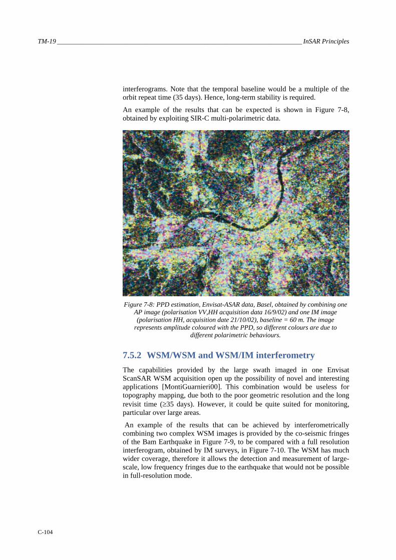
TM-19 _________________________________________________________________________ InSAR Principles
C-104
interferograms. Note that the temporal baseline would be a multiple of the orbit repeat time (35 days). Hence, long-term stability is required.
An example of the results that can be expected is shown in Figure 7-8, obtained by exploiting SIR-C multi-polarimetric data.
Figure 7-8: PPD estimation, Envisat-ASAR data, Basel, obtained by combining one
AP image (polarisation VV,HH acquisition data 16/9/02) and one IM image (polarisation HH, acquisition date 21/10/02), baseline = 60 m. The image
represents amplitude coloured with the PPD, so different colours are due to different polarimetric behaviours.
7.5.2 WSM/WSM and WSM/IM interferometry The capabilities provided by the large swath imaged in one Envisat ScanSAR WSM acquisition open up the possibility of novel and interesting applications [MontiGuarnieri00]. This combination would be useless for topography mapping, due both to the poor geometric resolution and the long revisit time (≥35 days). However, it could be quite suited for monitoring, particular over large areas.
An example of the results that can be achieved by interferometrically combining two complex WSM images is provided by the co-seismic fringes of the Bam Earthquake in Figure 7-9, to be compared with a full resolution interferogram, obtained by IM surveys, in Figure 7-10. The WSM has much wider coverage, therefore it allows the detection and measurement of large-scale, low frequency fringes due to the earthquake that would not be possible in full-resolution mode.

______________________________________________ Envisat-ASAR interferometric techniques and applications
C-105
Figure 7-9: Large scale (200 × 400 km), geocoded interferogram (absolute value coloured with phases), of the area of Bam (Iran), achieved by combining two
Envisat WS images acquired on 2 September 2003 and 8 June 2004, track 306. The normal baseline was 100 m and the scan patterns were synchronised up to 84%, leading to a resolution of approximately 40 m (range) × 150 m (azimuth). The
topographic contributions were removed by exploiting an SRTM DEM. The fringe contributions are mainly due to the earthquake of 26 December 2003 (some
atmospheric artefacts are still visible in the lower left part of the image).
Figure 7-10: Interferogram of BAM area, as in Figure 7-9, but achieved by combining two IM images: 3 December 2003 and 11 February 2004, with a
baseline close to zero. The interferogram resolution is pretty fine, approximately 20 × 10 m, but the ground coverage is much smaller than the previous image. The
different fringe pattern is due to the difference in the look angle.

TM-19 _________________________________________________________________________ InSAR Principles
C-106
Furthermore, the large WSM swath allows for frequent revisit-time monitoring. Such a system could be based on the mixed use of ScanSAR and full resolution images for WSM/IM interferometry. An example of a WSM/STRIPMAP interferogram is shown in Figure 7-11. The advantages of WSM/STRIPMAP versus WSM/WSM are twofold: firstly there is no need for scan pattern synchronisation; secondly there is much less volumetric decorrelation, provided that the optimal combination here discussed is used. The conclusion is that we have a higher probability of getting valuable information in this case than in WSM/WSM interferometry. However, the interferogram coverage would be the same as the STRIPMAP, and its resolution the same as the WSM.
Figure 7-11: Combined ScanSAR/STRIPMAP interferogram of the area around Las
Vegas. Left: fringes, right: detected amplitude, closeup of Las Vegas downtown. Topography has mostly been removed by exploiting an SRTM DEM: residual
fringes are thus mainly due to atmospheric effects.
We could likewise take advantage of the wide ScanSAR swath for frequent monitoring, in two different ways. A first system could provide alerts over hazardous areas. The use of WSM would reduce the revisit time to a few days due to the very large ScanSAR swath. Such a system would require that, for any new WSM acquisition, an IM with a suitable baseline has already been acquired over the same area. The number of IM images that must be previously acquired over the area of interest has been plotted in Figure 7-12 as a function of the revisit time and the orbit span.

______________________________________________ Envisat-ASAR interferometric techniques and applications
C-107
Figure 7-12: Number of images to be acquired to build the minimum database, computed here by assuming random orbit sampling and latitudes of 45o. The
number must be doubled to include ascending and descending orbits.
A second system could be provided by reversing the order of acquisitions. A first set of WSM images (the actual number is the same as in Figure 7-13) could be acquired over the area of interest in a short time. Thereafter, every new full resolution IM image could be combined with an WSM image in the database to get a (differential) interferogram. Such a system would be suitable to monitor large-scale changes like surface deformation, meteorological effect, Earth tides, according to user demand. The scheme of such a system is illustrated in Figure 7-13.
Figure 7-13: Monitoring system that exploits low and high-resolution acquisitions
to get short revisiting time intervals. Low and high resolution images correspond to WSM and IM acquisitions respectively.


______________________________________________________________________ ERS-Envisat interferometry
C-109
8. ERS-Envisat interferometry
8.1 Introduction Let us assume a combination of two monostatic SAR systems with slightly different central frequencies f0 and almost the same bandwidth W , such as ERS-2 (f0 = 5.3 GHz, W ≈ 16 MHz) and Envisat (f0 = 5.331 GHz, W ≈ 16 MHz). The two sensors could revisit the same areas, say after half an hour. This system would have very low temporal decorrelation, even better than the Tandem ERS mission, making the combination suitable for:
• High accuracy mapping on rolling topographies • Upgrading accuracy of the existing Tandem ERS1/2 DEM to a few cm,
and removing atmospheric artefacts
This frequency gap could be compensated by tuning the baseline, following the tuneable SAR idea [Prati94B, Gatelli94]. Hence, both super-resolution images and interferometry could be performed, as described in chapter C5. The trade-off between super-resolution and interferometry would be controlled by the baseline.
8.2 ERS-Envisat interferometric combination Figure 8-1 shows the ERS-Envisat interferometric geometry. The ERS-2 sensor operates at a slightly lower frequency than Envisat.
Figure 8-1: Geometry of the combined ERS-Envisat InSAR system.
R is the slant range axis, Bn the normal baseline, θ the incidence angle and α the terrain slope in range.

TM-19 _________________________________________________________________________ InSAR Principles
C-110
8.3 Frequency gap compensation The frequency gap can be compensated by exploiting the baseline. For interferometry, we require that the same wavenumber on the ground be illuminated by both sensors. According to Figure 8-2, Envisat can compensate for its intrinsic higher carrier frequency, fo = 5.33, by exploiting a lower incidence angle.
(a) (b)
Figure 8-2: (a) Spectral shift in MHz as a function of the range slope expressed for baselines from 1 km to 5 km. (b) Overlap of ERS and Envisat wave-number
spectrum at different baseline for flat terrain. Super-resolution × 2 is achieved when the two spectra are marginally overlapped, whereas full resolution interferometry
requires a complete overlap.
The baseline required to provide the proper wave-number shift on a ground terrain slanting at an angle α is:
of
fRB )tan( αθα
−Δ= Equation 8.1
The baseline Bα0 would generate a total spectral overlap of the two images and thus a constant phase interferogram with coherence γ = 1 in the absence of temporal variations and volume effects. Terrain slopes at range α ≠ αo would generate a relative spectral shift:
⎥⎦
⎤⎢⎣
⎡−
−−
Δ=Φ 1)tan()tan(),(
aaf o
o ϑϑαα Equation 8.2
As shown in Figure 8-2(a), if a 2000 metre baseline is adopted, a 5° slope in range would be perfectly compensated (no spectral shift) and slopes within the range ± 5° would have a spectral shift smaller than 10 MHz (about 2/3 of the system bandwidth W). Thus, if we assume rolling topography sites with gently varying slopes (i.e. almost constant within at least 3 consecutive pixels: about 75 m), and limited between ± 5°, an almost unitary coherence could be obtained on the entire image by means of the so called ‘common band filtering’ technique.

______________________________________________________________________ ERS-Envisat interferometry
C-111
8.4 Vertical accuracy The main advantage of such large-baseline interferometric combination lies in its intrinsic vertical accuracy. This accuracy can be computed by linking the standard deviation of the phase in Equation 1.18 with the phase standard deviation as a function of the coherence, γ , in Equation 1.16. We get an approximation for the standard deviation of the height:
BR
Nh πθλ
γγσ 4
sin2
1 2−= Equation 8.3
The coherence is expected to be good, due to the 1-day (or less) repeat pass interval. As an example, if we assume an overall coherence of γ = 0.5, and we average over N = 5 independent samples (i.e. a ground patch of ∼200 m2 on flat terrain), we get σφ ≅ 30 cm. The same accuracy would be achieved with a conventional Tandem interferogram (assuming Bn ≅ 200 m) by exploiting a ground patch that is 100 times bigger, e.g. 20 km2. However, in that case we would lose spatial accuracy.
8.5 Altitude of ambiguity Once the terrain slope α is compensated by means of the baseline Bα , the altitude of ambiguity ha can be computed similarly to the section 2:
α
αθBf
cRho
a 2)sin( −
= Equation 8.4
Then, by substituting the expression of the compensation baseline Bα , given by 8.1, we get the following simple expression:
fcha Δ
−=
2)cos( αθ
Equation 8.5
In the case of ERS-Envisat interferometry the following expression of the altitude of ambiguity (in metres) holds:
)cos(510312
)cos(1036
8
αθαθ−≅
⋅⋅−⋅
=ah Equation 8.6
As an example, if we consider a terrain slope of 2.5% (about 1.5°), the altitude of ambiguity would be about 4.6 metres. It should be noted that with such a small altitude of ambiguity compared with the pixel size (25 × 5 m range/azimuth) the resulting interferogram (even if strongly coherent) would be difficult to unwrap, especially in the azimuth direction where the terrain slope is not compensated. Nonetheless, the main application of this system would be the improvement of the accuracy of the low spatial frequencies of an existing DEM (e.g. generated from ERS Tandem images). Thus, the existing DEM could be used to demodulate the ERS-Envisat interferogram and the residue could be low-pass filtered, thus improving the coherence, which might be low due to temporal changes and volume scattering.

TM-19 _________________________________________________________________________ InSAR Principles
C-112
8.6 Effect of volume scattering Due to terrain roughness around the slope α0 compensated with the baseline Bα 0, the interferogram coherence decreases. We can refer to the volume scattering decorrelation computed in Equation 1.28:
2221 ⎟⎟
⎠
⎞⎜⎜⎝
⎛−≅
a
zz h
σπγ Equation 8.7
In the case of interest for us, i.e. ha = 4.6 m, either σ z < 0.6 m, or Δz << 2 m. These conditions are rather stringent, but are likely to be satisfied in flat areas or in rolling topography.
8.7 Experimental results Notwithstanding the problems due to the unavailability of ERS-2 gyros, experimental evidence for the possibility of generating a SAR-ERS/ASAR-Envisat interferogram can be provided. The main goal of this experiment was to quantify the actual vertical accuracy of an ERS-Envisat interferometric DEM of a rural area along the rivers Réveillon and Yerres (tributaries of Seine) in the immediate neighbourhood of Paris. Second was to show that with a 30' temporal baseline and 1.5 km geometric baseline, neat fringes can be obtained on vegetated areas, whereas a random location phase screen is obtained on urban areas. Following the spectral shift theory, it should be pointed out that with a normal baseline of about 1.5 km the 30 MHz frequency shift can be practically compensated on cross-track terrain slopes ranging from –1 to 8 degrees. Moreover, in our data the DC difference was found to be about 800 Hz, thus leaving a common band in azimuth slightly greater than 20% of the ERS Pulse Repetition Frequency (see Figure 8-3).
Figure 8-3: SAR-ERS and ASAR-Envisat azimuth spectra. The resulting azimuth
common band is about 20% of the ERS pulse repetition frequency.

______________________________________________________________________ ERS-Envisat interferometry
C-113
The unfiltered interferogram that was obtained after accurate image registration, and its azimuth common band filtered version, are shown in Figure 8-4.
Figure 8-4: Left: unfiltered interferogram obtained after accurate ERS-Envisat image registration. Right: The
interferometric fringes after the azimuth common band filtering.
The slant range common band filtered interferogram is shown in Figure 8-5.
Figure 8-5: Left: The ERS-Envisat interferometric fringes after slant-range common band filtering. Right: Local
ground range slope estimated from the local spectral shift that maximises the local coherence.
Due to the 1.5 km baseline, the altitude of ambiguity is about 6 m. The map of the ground range slope shown in Figure 8-5 has been derived from the value of frequency (changed by means of the common band filtering described above) that maximises the local complex coherence (an approximation of the optimal estimator in section 2.3).

TM-19 _________________________________________________________________________ InSAR Principles
C-114
Figure 8-6 shows a detail of the ERS-Envisat interferometric fringes of the rural area including the rivers Réveillon and Yerres. On this area the coherence and the relative elevation standard deviation histogram have been computed.
Figure 8-6: Detail of the ERS-Envisat interferometric fringes of the rural area
including the rivers Reveillon and Yerres
The two histograms are shown in Figure 8-7. Here it is possible to appreciate the very high vertical accuracy that can be obtained by combining ERS-2 and Envisat SAR images.
Figure 8-7: Left: Coherence histogram of the area shown in Figure 8-6. Right:
Histogram of the elevation accuracy derived from the coherence map shown on the left.
Finally, the ERS-Envisat interferogram of Paris is shown in Figure 8-8. Here it is interesting to note that neat fringes are clearly visible on the city parks (the 30' temporal baseline avoids temporal decorrelation), whereas on the urbanised areas an almost random phase field (the location phase screen of point scatterers) is present. This is exactly the opposite of what we are familiar with from ERS/ERS interferograms (small geometric and large

______________________________________________________________________ ERS-Envisat interferometry
C-115
temporal baselines), and it highlights the kind of applications the technique would lead to.
Figure 8-8: The left part of the image is centred on Paris. Here neat fringes are
clearly visible on the city parks, whereas on the urbanised areas an almost random phase field is present.