Working with Data and Charts

In Excel, a formula calculates a value based on the values in other cells of theworkbook. Excel displays the result of a formula in a cell as a numeric value.

A function is an abbreviated formula that performs a specific operation on agroup of values. Excel provides more than 250 functions that can help youwith tasks ranging from determining loan payments to calculating investmentreturns.

You’ve already learned the fundamentals of creating a worksheet, so now youcan concentrate on some of the other features that add to the data presenta-tion. For example, you can create a chart based on data in a worksheet.Charts are very useful for interpreting data; however, different people look atdata in different ways. To account for this, you can quickly change the appear-ance of charts in Excel by clicking directly on the chart. You can change titles,legend information, axis points, category names, and more.

The axes are the grid on which the data is plotted. On a 2D chart, the y-axis isthe vertical axis on a chart (the value axis) and the x-axis is the horizontal axis(the category axis). A 3D chart has these two axes, plus a z-axis. You can con-trol all the aspects of the axes—the appearance of the line, the tick marks, thenumber format used, and more.

PA

RT 9

09 0789729628 CH09 8/21/03 1:26 PM Page 140

Formatting Numbers andCharts

GeneralCurrencyPercentCommaOne decimalplace

Three decimalplaces

Chart toolbar

Legend

ChartX-axis

AutoSumCalculation

Date

Function

Functionresult

Chart title

Y-axis

09 0789729628 CH09 8/21/03 1:26 PM Page 141

Start

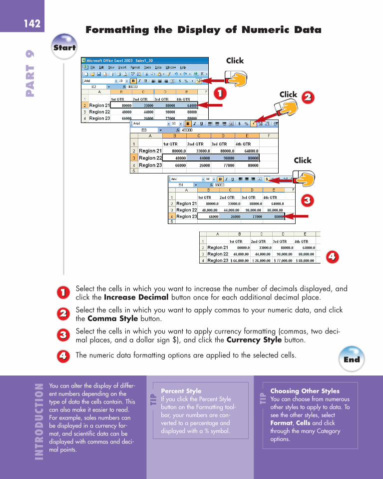
Select the cells in which you want to increase the number of decimals displayed, andclick the Increase Decimal button once for each additional decimal place.

Select the cells in which you want to apply commas to your numeric data, and clickthe Comma Style button.

Select the cells in which you want to apply currency formatting (commas, two deci-mal places, and a dollar sign $), and click the Currency Style button.

The numeric data formatting options are applied to the selected cells.

142PA

RT 9

Formatting the Display of Numeric Data

22

33

33

44

11

11

INTR

OD

UCT

ION

TIP

TIPPercent Style

If you click the Percent Stylebutton on the Formatting tool-bar, your numbers are con-verted to a percentage anddisplayed with a % symbol.

You can alter the display of differ-ent numbers depending on thetype of data the cells contain. Thiscan also make it easier to read.For example, sales numbers canbe displayed in a currency for-mat, and scientific data can bedisplayed with commas and deci-mal points.

Choosing Other StylesYou can choose from numerousother styles to apply to data. Tosee the other styles, selectFormat, Cells and clickthrough the many Categoryoptions.

End

22

44

Click

Click

Click

09 0789729628 CH09 8/21/03 1:26 PM Page 142

Start

143Performing Calculations with AutoSum

Click the cell in which you want the AutoSum function to appear.

Click the AutoSum button on the Standard toolbar and select the preferred functionfrom the drop-down list (in this example, Sum).

If Excel automatically selected the correct range (the selected range is surrounded witha flashing dotted line), press the Enter key. If not, see the tip at the bottom of the page.

Click the cell containing the function. Notice that the formula is displayed in theFormula bar.

INTR

OD

UCT

ION

TIP

Selecting Specific AutoSum CellsIf you don’t want to use the range of cells AutoSum selects for you, clickthe first cell you want, hold down the Ctrl key, and click each additionalcell you want to include in the calculation. When you finish selecting thecells you want to calculate, press Enter. For more information on select-ing cells, see “Selecting Cells” and “Selecting a Range of Cells” in Part7, “Getting Started with Excel.”

Excel can use formulas and func-tions to perform calculations foryou. Because a formula refers tothe cells themselves rather than tothe values they contain, Excelupdates the sum whenever youchange the values in the cells.You’ll probably use the AutoSumformula frequently—it adds num-bers in a range of cells.

End

22

22

33

44

44

11

11

33

Click

Click

Click

09 0789729628 CH09 8/21/03 1:26 PM Page 143

Start

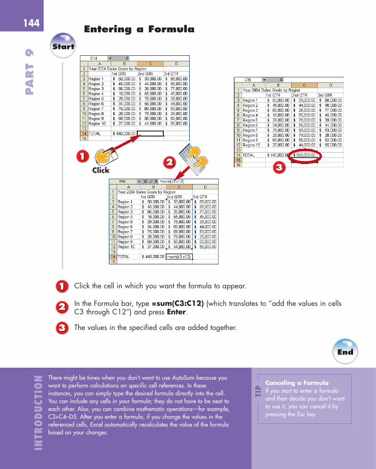
Click the cell in which you want the formula to appear.

In the Formula bar, type =sum(C3:C12) (which translates to “add the values in cellsC3 through C12”) and press Enter.

The values in the specified cells are added together.

144PA

RT 9

Entering a Formula

22

22

33

11

11

INTR

OD

UCT

ION

TIP

There might be times when you don’t want to use AutoSum because youwant to perform calculations on specific cell references. In theseinstances, you can simply type the desired formula directly into the cell.You can include any cells in your formula; they do not have to be next toeach other. Also, you can combine mathematic operations—for example,C3+C4–D5. After you enter a formula, if you change the values in thereferenced cells, Excel automatically recalculates the value of the formulabased on your changes.

Canceling a FormulaIf you start to enter a formulaand then decide you don’t wantto use it, you can cancel it bypressing the Esc key.

End

Click 33

09 0789729628 CH09 8/21/03 1:26 PM Page 144

HIN

T

Start

145Copying a Formula

Select the cell that contains the formula you want to copy, and click the Copy buttonon the Standard toolbar.

Select the cell (or multiple cells) into which you want to paste the formula, and clickthe Paste button.

The formula automatically performs the calculation on similarly located data, placingthe results into the selected cell(s).

INTR

OD

UCT

ION

TIP

Order of OperationExcel first performs any calcula-tions within parentheses. Then,it performs multiplication ordivision calculations, from leftto right. Finally, it performs anyaddition or subtraction, fromleft to right.

When you build your worksheet,you might want to use the samedata and formulas in more thanone cell. With Excel’s Copy com-mand, you can create the initialdata or formula once and thenplace copies of this information inthe appropriate cells.

End

22

22

33

11

11Click

Click

33

09 0789729628 CH09 8/21/03 1:26 PM Page 145

Start

Select the cell in which you want the function to appear, and click the InsertFunction button to open the Insert Function dialog box.

If you don’t know the name of the function you want to use, type a brief descriptionof it in the Search for a Function box and click Go.The recommended function (in this case, PMT) is highlighted in the Select a Function list.Read the function’s description to ensure that it’s the one you want. If so, double-click it.

The Function Arguments dialog box opens. Click in the Rate field and type, forexample, .06/12 for a 6% interest loan with monthly payments.

146PA

RT 9

Entering a Function

22

22

33

33

44

11

11

INTR

OD

UCT

ION

TIP

A function is one of Excel’s many built-in formulas for performing a spe-cialized calculation on the data in your worksheet. For example, insteadof totaling your sales data, suppose you want to determine the averageof each quarter per region (the Average function), the highest sales num-bers for the year (the Max function), or the lowest sales numbers for theyear (the Min function). Or perhaps, as in this task, you want to findhow much your payment would be on a home loan given a specificinterest rate (Rate), number of periods (Nper), and price (Present Value).(Note that this calculates only the principal and interest portion for yourhome loan payment [PMT]).

Opening the InsertFunction Dialog BoxYou can also select AutoSum,More Functions on the Standardtoolbar to open the InsertFunction dialog box, or youcan select Insert, Function.

Click

Double-click

Click

44

09 0789729628 CH09 8/21/03 1:26 PM Page 146

TIP

The Function ArgumentsDialog BoxPractice using the many func-tions offered in the FunctionArguments dialog box, and seethe results you get from yourcalculations. You can move theFunction Arguments dialog boxaround to better see your cells.

147

Assuming the loan is a 30-year loan, click in the Nper field and type, for example,360 (12 months times 30 years on the loan).

Click in the Pv field and type 200000 for a $200,000 loan. You can leave anyfields blank that are not bolded.

Click OK.

The calculation of the payment function is displayed in the cell and in the Formulabar. End

66

77

77

88

88

55

TIP

Entering ArgumentsAn argument is anything used in the function to produce the end result.As you enter information into the Function Arguments dialog box, readthe argument descriptions that appear. If, after reading an argument’sdescription, you still aren’t sure what you should enter, click the Helpon This Function link in the bottom-left corner of the dialog box.

Click

55

66

09 0789729628 CH09 8/21/03 1:26 PM Page 147

Start

Click a cell with a #VALUE! message and review the cell’s formula in the Formulabar. Can you find the error?

To add the values C2 through C12 and divide by 10, the formula must include“SUM” in the function. Type SUM in the Formula Bar and press Enter.Click a cell with a #NAME? message. Move the mouse pointer over the cell toreview a ScreenTip about the error.

148PA

RT 9

Correcting Formula and Function Errors

22

33

33

11

11

INTR

OD

UCT

ION

TIP

Tracing ErrorsCheck formulas by tracingprecedents (all cells that are ref-erenced [in order] in the for-mula). You can also tracedependents (start with a cellthat is referenced in a formula,and then trace all the cells thatreference that cell).

Excel notifies you when there are errors in your data by displaying dif-ferent error descriptions. #VALUE? means the formula in the cell con-tains either nonnumeric data or cell/function names that cannot be usedin the calculation. #NAME? means the formula contains incorrectlyspelled cell/function names. #REF! indicates that the formula contains areference to a cell that isn't valid. #### means the column is not wideenough to display the data. #DIV/0! means that the formula is trying todivide a number by 0 or that the formula is referencing an empty cell.

Click

Click

22

09 0789729628 CH09 8/21/03 1:26 PM Page 148

HIN

T

End

TIP

Performing a Trace Click the cell with the error,select Tools, FormulaAuditing, and select eitherTrace Precedents or TraceDependents.

149

In this example, avg is not the correct name of the desired function; the correct nameis average. In the Formula bar, replace avg with average and press Enter.

If the status bar displays a Circular reference error (for example, Circular: D15),double-click the cell it references.

In this case, the formula is referencing its own cell. Type the correct formula in theFormula bar (in this example, =SUM(D3:D12)/10) and press Enter.

If a cell displays #####, the column isn’t wide enough to display all the cell‘s data.Click and drag the column border to make it wider, and the error is gone.

66

77

55

TIP

Circular ReferencesThe formula for cell E15 in this task is the average for fourth-quartersales for the 10 regions, displayed as follows: =E14/10. If you insteadwrote this formula as =E3:E12/10, it would still be correct (E14 justhappens to be the total for the regions). But, if you accidentally wrote=E3:E15/10, including the cell in which you want the answer, therewould be a circular reference. You cannot produce an answer for cellE15 while including it in the calculation; the answer would go roundand round, continuously changing—hence the name circular reference.

44

Double-click

Drag55

77

44

66

09 0789729628 CH09 8/21/03 1:26 PM Page 149

Start

Select the cells you want to include in your chart, and click the Chart Wizard but-ton on the Standard toolbar.

The first page of the Chart Wizard opens. Select a type from the Chart Type listand the Chart Sub-type list; then click Next.

Depending on how you want your information to display in the chart, select eitherRows or Columns in the Series in area; then click Next.

150PA

RT 9

Inserting Charts

22

33

11

INTR

OD

UCT

ION

TIP

Viewing a SampleThe Chart Wizard enables youto select how your data lookswith a chart type and subtype.To do so, move your mousepointer over the Press andHold to View Sample but-ton and then press and holddown the left mouse button.

Interpreting numeric data by looking at numbers in a table can be diffi-cult. Using data to create charts can help people visualize the data’s sig-nificance. For example, you might not have noticed in a spreadsheet thatthe same month of every year has low sales figures, but it becomes obvi-ous when you make a chart from the data in that spreadsheet. Thechart’s visual nature also helps others review your data without the needto review every single number.

11

2233

Click

Click

Click

09 0789729628 CH09 8/21/03 1:26 PM Page 150

TIP

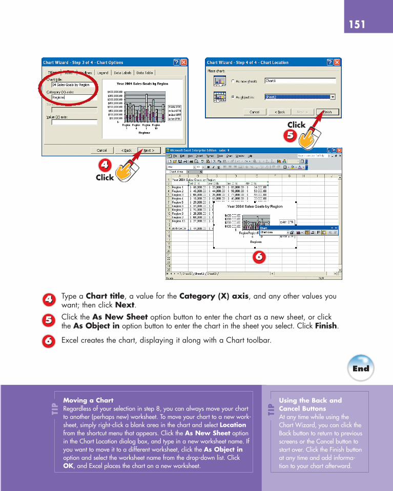
Moving a ChartRegardless of your selection in step 8, you can always move your chartto another (perhaps new) worksheet. To move your chart to a new work-sheet, simply right-click a blank area in the chart and select Locationfrom the shortcut menu that appears. Click the As New Sheet optionin the Chart Location dialog box, and type in a new worksheet name. Ifyou want to move it to a different worksheet, click the As Object inoption and select the worksheet name from the drop-down list. ClickOK, and Excel places the chart on a new worksheet.

TIP

Using the Back andCancel ButtonsAt any time while using theChart Wizard, you can click theBack button to return to previousscreens or the Cancel button tostart over. Click the Finish buttonat any time and add informa-tion to your chart afterward.

151

Type a Chart title, a value for the Category (X) axis, and any other values youwant; then click Next.Click the As New Sheet option button to enter the chart as a new sheet, or clickthe As Object in option button to enter the chart in the sheet you select. Click Finish.

Excel creates the chart, displaying it along with a Chart toolbar.

End

66

55

44

Click

66

55

44

Click

09 0789729628 CH09 8/21/03 1:26 PM Page 151

HIN

T

End

Start

Click the Chart Objects down arrow and select the object in the chart you want toedit (scroll through the list if necessary).

After you select the object, for example, the Category Axis, you can use the otherbuttons on the Chart toolbar to make changes to it.Move the mouse pointer over the rest of the buttons on the Chart toolbar to seeScreenTips of the other types of edits you can make to your chart.

Format the object, alter the chart type, add a legend and/or data table, swap the series data by row or by column, and change text objects’ direction angle.

152PA

RT 9

Editing Charts with the Chart Toolbar

22

33

44

11

INTR

OD

UCT

ION

TIP

Double-Clicking the ChartOne of the fastest ways to edita chart’s options is to double-click the element in the chartyou want to alter. The appropri-ate dialog box opens, enablingyou to make the changes youneed.

Charts are useful for interpreting data, but different people look at data indifferent ways. To accommodate different users, you can change titles, leg-end information, axis points, category names, and more. The Charttoolbar—which you can activate by opening the View menu and selectingToolbars, Chart—lists all the items in your chart that you can alter. Simplyindicate which chart object you want to alter, and then click the appropriatebutton. If you don’t know the name of the item you want to format on yourchart, simply click the object on the chart and the name will appear in theChart Objects list box on the Chart toolbar.

22

33

44

11

Click

Click

09 0789729628 CH09 8/21/03 1:26 PM Page 152

Start

153

End

TIP

HIN

TTurning Off AutoCalculateAutoCalculate continues towork until you turn it off. Youcan turn off the AutoCalculatefeature by selecting None fromthe AutoCalculate shortcutmenu.

33

33

Select the cells you want to AutoCalculate.

Right-click the status bar and select the AutoCalculate option from the shortcutmenu. (The default AutoCalculate operation is to sum the numbers.)

Using AutoCalculate

22

22

11

INTR

OD

UCT

ION Suppose you want to see a func-

tion performed on some of yourdata—in this example, to deter-mine the lowest quarterly salesgoal of any region in 2004—butyou don’t want to add the functiondirectly into the worksheet. Excel’sAutoCalculate feature can help.

11

Click

Right-Click

The status bar displays the selected calculation, for example, the lowest number inthe selection (Min = $18,000.00).

09 0789729628 CH09 8/21/03 1:26 PM Page 153

HIN

T

Start

Select a cell in the column you want sorted alphabetically or numerically (dependingon whether the sort column contains text data or numeric data).

Click the Sort Ascending button on the Standard toolbar.

The data is sorted alphabetically from A to Z or numerically from the lowest amountto the highest. Click the Sort Descending button.

This sorts the data alphabetically from Z to A, or numerically from the highestamount to the lowest.

154PA

RT 9

Sorting Data Lists

22

33

44

11

INTR

OD

UCT

ION

TIP

Sorting on Multiple ColumnsTo sort on multiple columns of data, select Data, Sort to open the Sortdialog box. Select the first Sort by column name (for example,Region) from the drop-down list box; then choose up to two moreoptions from the Then by drop-down list box (for example, YTDSales). Make sure you indicate whether you have a header row (if not,the columns will list as Column1, Column2, and so on), and click theOK button to perform the sort on your data.

You can easily change the orderof the data in your worksheet. If,for example, you want to alpha-betically arrange the names in adata list of sales representatives,you can sort on Last Name.Alternatively, you might want tosort your sales representatives bythe region in which they work orby YTD sales.

End

22

33

11

44

Click

Click

09 0789729628 CH09 8/21/03 1:26 PM Page 154

Start

155Freezing Rows and Columns

Click the cell to the right of and below the area you want to freeze. (Typically, this iscell B2 if your main header row is Row 1 and your main column is Column A.)

Open the Window menu and select Freeze Panes.

Move through the worksheet using the arrow keys on your keyboard. Frozen Row 1and Column A enables you to view your data without losing sight of the titles.

Open the Window menu and select Unfreeze Panes to unfreeze the columns androws.

INTR

OD

UCT

ION

TIP

Splitting a WorksheetBy splitting a worksheet, you can scroll independently into different hori-zontal and vertical parts of a worksheet. This is useful if you want toview different parts of a worksheet or copy and paste between differentareas of a large worksheet. Simply unfreeze the panes, and then openthe Window menu and select Split. You can move the split bars byclicking and dragging them as necessary.

Many of your worksheets mightbe large enough that you cannotview all the data onscreen at thesame time. In addition, if theworksheet contains row or columntitles and you scroll down or tothe right, some of the titles are toofar to the top or left of the work-sheet for you to see.

End

22

33

44

11

11

33Click

Click 22

44Click

09 0789729628 CH09 8/21/03 1:26 PM Page 155