3. Peano Arithmetic

3.1. Language and Axioms.

Definition 3.1. The language of arithmetic consists of:

• A 0-ary function symbol (i.e. a constant) 0,• A unary function symbol S,• Two binary function symbols +, ·,• Two binary relation symbols =, <,• For each n, infinitely many n-ary predicate symbols Xi

n.

We often abbreviate ¬(x = y) by x 6= y and sometimes ¬(x < y) byx 6< y. We write x ≤ y as an abbreviation for x < y ∨ x = y and s+ t, s · tas “abbreviations” for +st and ·st.

We intend these symbols to represent their usual meanings regardingarithmetic. S is the successor operation. The predicate symbols Xi

n in-tentionally have no fixed meaning; their purpose is so that if we prove aformula φ containing one of them then not only have we proven φ[ψ/Xi

n](the formula where we replace Xi

n with the formula ψ) for any ψ in ourlanguage, we have proven φ[ψ/Xi

n] for any formula in any extension of thelanguage of arithmetic.

Definition 3.2. P− consists of formulas:

• ∀x(x = x),• ∀x∀y(x = y → φ[x/z]→ φ[y/z]) where φ is atomic and x and y are

substitutable for z in φ,• ∀x(Sx 6= 0),• ∀x∀y(Sx = Sy → x = y),• ∀x∀y(x < Sy ↔ x ≤ y),• ∀x(x 6< 0),• ∀x∀y(x < y ∨ x = y ∨ y < x),• ∀x(x+ 0 = x),• ∀x∀y(x+ Sy = S(x+ y)),• ∀x(x · 0 = 0),• ∀x∀y(x · Sy = x · y + x).

The second equality axiom is a bit subtle. In particular, note that φ isallowed to contain x or y, so we can easily derive

x = y → x = x→ y = x

(taking φ to be z = x) and

y = x→ y = w → x = w

(taking φ to be z = w).Finally, in order to prove anything interesting, we need to add an induc-

tion scheme.1

2

Definition 3.3. The axioms of arithmetic, ΓPA, consist of P− plus, forevery formula φ and each variable x, the formula

φ[0/x]→ ∀x(φ→ φ[Sx/x])→ ∀xφ.We write PA ` Γ ⇒ Σ if Fc ` ΓPAΓ ⇒ Σ and HA ` Γ ⇒ Σ if Fi `

ΓPAΓ⇒ Σ.

PA stands for Peano Arithmetic while HA stands for Heyting arithmetic.

Definition 3.4. The numerals are the terms built only from 0 and S. If nis a natural number, we write n for the numeral given recursively by:

• 0 is the term 0,• n+ 1 is the term Sn.

3.2. Basic Properties. We will generally not try to give even simple proofsexplicitly in the sequent calculus: even very simple arguments rapidly be-come infeasible. (Consider, for example, that the most basic argumentsinvolving substitution generally take several inference rules.)

Instead, we will accept from our previous work that Fc already capturesmost ordinary logical reasoning, and we will give careful arguments from theaxioms, using informal logic.

Theorem 3.5. HA proves that additition is commutative:

∀x∀y x+ y = y + x.

Proof. By induction on x. It suffices to show ∀y 0+y = y+0 and ∀y(x+y =y + x)→ ∀y(Sx+ y = y + Sx).

For the first of these, since y + 0 = y, it suffices to show that 0 + y = y;we show this by induction on y. 0 + 0 = 0 is an instance of an axiom, andif 0 + y = y then 0 + Sy = S(0 + y) = Sy.

Now assume that ∀y(x + y = y + x). Again, we go by induction on y.Sx + 0 = Sx and we have already shown that 0 + Sx = Sx. SupposeSx+ y = y + Sx; then

Sx+Sy = S(Sx+y) = S(y+Sx) = SS(y+x) = SS(x+y) = S(x+Sy) = S(Sy+x) = Sy+Sx.

(Consider just how many infence rules it would take to completely formalizeapplying the transitivity of = over seven equalities, which forms only one ofthe three inductive arguments in the proof.) �

By similar arguments, HA (and so also PA) proves all the standard factsabout the arithmetic operations. These systems are (more than) strongenough to engage in sensible coding of more complicated (but still finite)objects. The details of how to accomplish this sort of coding are tedious andsufficiently described elsewhere, but we will briefly describe what it meansto code something in the language of arithmetic with an example.

One of the first things that needs to be coded is the notion of a finitesequence of natural numbers. What we mean by this is that we wish toinformally set up a correspondence between finite sequences and natural

3

numbers. Let us name a function π which is an injective map from finitesequences to natural numbers. The range of π should be definable; that is,there should be a formula φπ such that HA ` φπ(n) when n = π(σ) forsome σ and HA ` ¬φπ(n) when n is not in the range of π.

Then we need the natural operations on sequences to be definable. Forinstance, we would like to be able to take a sequence σ and a natural num-ber n and define the sequence σ_〈n〉 which consists of appending n to thesequence σ. To code this, we should have a formula φ_ such that:

• If m = π(σ_〈n〉) then HA ` φ_(π(σ), n,m),

• If m 6= π(σ_〈n〉) then HA ` ¬φ_(π(σ), n,m),• HA ` ∀x, y, z, z′(φ_(x, y, z) ∧ φ_(x, y, z′)→ z = z′), and• HA ` ∀x, y(φπ(x)→ ∃zφ_(x, y, z)).

The first two clauses state the HA proves that φ_ correctly identifiesπ(σ_〈n〉) for actual sequences σ and natural numbers n. But this isn’tenough to give the last two clauses, because HA can’t actually prove thatthe numerals n are the only numbers. So the last two clauses say that HAcan actually prove that φ_ represents a well-defined function. (For instance,the last two clauses ensure that in a nonstandard model, which has “non-standard sequences”, the _ operation still has a sensible interpretation.)

Coding sequences is crucial to the power of HA because we can carry outinduction along sequences. In particular, this lets us define exponentiation:we say x = yz if there is a sequence σ of length z such that σ(0) = y,σ(i + 1) = σ(i) · y for each i, and the last element of σ is equal to x. Andonce we have done this, we could define iterated exponentiation, and so on.

Once we can code sequences, it also becomes much easier to define othernotions, since we can use sequences to combine multiple pieces of informationin a single number. For instance, we could define a finite group to consist ofa quadruple 〈G, e,+G,

−1〉 where G is a number coding a finite set, e is anelement of G, +G and −1 are numbers coding finite sets of pairs, and thenwrite down a long formula describing what has to happen for this quadrupleto properly define a group.

To illustrate just how much is provable, we quote Harvey Friedman’s“grand conjecture”

Every theorem published in the Annals of Mathematics whosestatement involves only finitary mathematical objects (i.e.,what logicians call an arithmetical statement) can be provedin EFA. EFA is the weak fragment of Peano Arithmetic basedon the usual quantifier-free axioms for 0, 1, +, , exp, togetherwith the scheme of induction for all formulas in the languageall of whose quantifiers are bounded.

(We will define the notion of a bounded quantifier below.) In other words,almost all of conventional combinatorics, number theory, finite group theory,and so on can be coded up and then proven, not only inside PA, but in acomparatively small fragment of PA. (Later on we’ll have a way to quantify

4

how strong fragments of PA are, and we’ll learn that EFA is very smallindeed.)

3.3. The Arithmetical Hierarchy.

Definition 3.6. We write ∀x < y φ as an abbreviation for ∀x(x < y → φ)and ∃x < y φ as an abbreviation for ∃x(x < y ∧ φ).

Note that PA ` ¬∀x < y ¬φ↔ ∃x < y φ and PA ` ¬∃x < y ¬φ↔ ∀x <y φ, just as we would expect. We call these bounded quantifiers. As we willsee, formulas in which all quantifiers are bounded behave like quantifier-freeformulas. We call other quantifiers unbounded.

Because HA can describe sequences in a single number, there is no realdifference between a single quantifier ∃x and a block of quantifiers of thesame type, ∃x1∃x2 · · · ∃xn—anything said with the later could be coded upand expressed with a single quantifier. Furthermore, all the coding necessarycan be done using only bounded quantifiers. Therefore we will generallysimply write a single quantifier, knowing that it could stand for multiplequantifiers of the same type.

Definition 3.7. The ∆0 formulas are those in which all quantifiers arebounded. Σ0 and Π0 are alternates names for ∆0.

The Σn+1 formulas are formulas of the form

∃xφ(possibly with a block of several existential quantifiers) where φ is Πn.

The Πn+1 formulas are formulas of the form

∀xφ(possibly with a block of several universal quantifiers) where φ is Σn.

In particular, the truth of ∆0 formulas is computable, in the sense thatgiven numeric values for the free variables in ∆0, we can easily run a com-puter program which checks in finite time whether the formula is true (underthe intended interpretation in the natural numbers).

By the same argument that shows every formula is equivalent in Fc toa prenex formula, PA shows that every formula is equivalent to a formulawith its unbounded quantifiers in front, which must be Σn or Πn for somen.

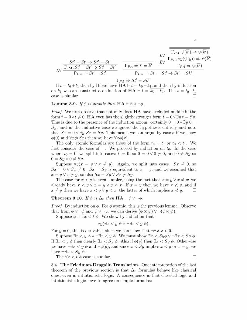
Lemma 3.8. If t is a closed term then there is a natural number k suchthat HA ` t = k.

Proof. By induction on the construction of the term t. If t = 0 then this istrivial since 0 = 0 is derivable.

If t = St′ then by IH we have HA ` t′ = k′, and therefore we can deriveSt′ = Sk′. To keep the formula managable, we write ψ(t) as an abbreviationfor t′ = t → St′ = St′ → St′ = St. Note that this is an instance of thesubstitution axiom.

5

St′ = St′ ⇒ St′ = St′

ΓPA, St′ = St′ ⇒ St′ = St′

L∀ΓPA ⇒ St′ = St′

ΓPA ⇒ t′ = k′

ΓPA, ψ(k′)⇒ ψ(k′)L∀

ΓPA, ∀y(ψ(y))⇒ ψ(k′)L∀

ΓPA ⇒ ψ(k′)

ΓPA ⇒ St′ = St′ → St′ = Sk′

ΓPA ⇒ St′ = Sk′

If t = t0+ t1 then by IH we have HA ` t = k0+k1, and then by inductionon k1 we can construct a deduction of HA ` t = k0 + k1. The t = t0 · t1case is similar. �

Lemma 3.9. If φ is atomic then HA ` φ ∨ ¬φ.

Proof. We first observe that not only does HA have excluded middle in theform t = 0∨t 6= 0, HA even has the slightly stronger form t = 0∨∃y t = Sy.This is due to the presence of the induction axiom: certainly 0 = 0∨∃y 0 =Sy, and in the inductive case we ignore the hypothesis entirely and notethat Sx = 0 ∨ ∃y Sx = Sy. This means we can argue by cases: if we showφ(0) and ∀xφ(Sx) then we have ∀xφ(x).

The only atomic formulas are those of the form t0 = t1 or t0 < t1. Wefirst consider the case of =. We proceed by induction on t0. In the casewhere t0 = 0, we split into cases: 0 = 0, so 0 = 0 ∨ 0 6= 0, and 0 6= Sy so0 = Sy ∨ 0 6= Sy.

Suppose ∀y(x = y ∨ x 6= y). Again, we split into cases. Sx 6= 0, soSx = 0 ∨ Sx 6= 0. Sx = Sy is equivalent to x = y, and we assumed thatx = y ∨ x 6= y, so also Sx = Sy ∨ Sx 6= Sy.

The case for x < y is even simpler, using the fact that x = y ∨ x 6= y: wealready have x < y ∨ x = y ∨ y < x. If x = y then we have x 6< y, and ifx 6= y then we have x < y ∨ y < x, the latter of which implies x 6< y. �

Theorem 3.10. If φ is ∆0 then HA ` φ ∨ ¬φ.

Proof. By induction on φ. For φ atomic, this is the previous lemma. Observethat from φ ∨ ¬φ and ψ ∨ ¬ψ, we can derive (φ~ ψ) ∨ ¬(φ~ ψ).

Suppose φ is ∃x < t φ. We show by induction that

∀y(∃x < y φ ∨ ¬∃x < y φ).

For y = 0, this is derivable, since we can show that ¬∃x x < 0.Suppose ∃x < y φ ∨ ¬∃x < y φ. We must show ∃x < Syφ ∨ ¬∃x < Sy φ.

If ∃x < y φ then clearly ∃x < Sy φ. Also if φ(y) then ∃x < Sy φ. Otherwisewe have ¬∃x < y φ and ¬φ(y), and since x < Sy implies x < y or x = y, wehave ¬∃x < Sy φ.

The ∀x < t φ case is similar. �

3.4. The Friedman-Dragalin Translation. One interpretation of the lasttheorem of the previous section is that ∆0 formulas behave like classicalones, even in intuitionistic logic. A consequence is that classical logic andintuitionistic logic have to agree on simple formulas:

6

Theorem 3.11. If φ is Π2 and PA ` φ then HA ` φ.

This statement is not true if we deduce a sequent of Π2 formulas insteadof a single formula.

For the proof, we need another translation of formulas:

Definition 3.12. Fix a formula θ.

• ⊥FD is θ,• If p is atomic and not ⊥, pFD is p ∨ θ,• (φ~ ψ)FD is φFD ~ ψFD,• (Qxφ)FD is Qx(φFD).

Note that this is the result of the ∗ translation from intuitionistic tominimal logic followed by replacing every occurrence of ⊥ with θ.

Lemma 3.13. If Fm ` Γ⇒ Σ and Γ[θ/⊥],Σ[θ/⊥] are the result of replacingevery occurrence of ⊥ with the formula θ, then Fm ` Γ[θ/⊥]⇒ Σ[θ/⊥].

Proof. Proof sketch: This follows from the fact that ⊥ has no special prop-erties in minimal logic. We proceed by induction on deductions, and theonly way ⊥ can be introduced is by weakening or by the axiom ⊥ ⇒ ⊥. �

Theorem 3.14. If HA ` Γ⇒ Σ then HA ` ΓFD ⇒ ΣFD.

Proof. We proved for first-order logic in general that if Fi ` ΓPA,Γ ⇒ Σthen Fm ` Γ∗A,Γ

∗ ⇒ Σ∗. The previous lemma then shows that Fm `ΓFDPA ,Γ

FD ⇒ ΣFD.Furthermore, we have already seen that Fi ` φ → φ∗, and by the same

argument, Fi ` φ → φFD. In particular, we may apply cuts over all theaxioms of ΓPA actually used in the original proof to obtain Fi ` ΓPA,Γ

FD ⇒ΣFD, and therefore HA ` ΓFD ⇒ ΣFD. �

Lemma 3.15. If φ is ∆0 and no free variable in θ appears bound in φ thenHA ` φFD → φ ∨ θ.

Proof. By induction on φ. If φ is ⊥, this is trivial since ⊥FD is θ. If φ isatomic then φFD is exactly φ ∨ θ.

If φ = ψ0 ∨ ψ1, it is easy to derive ψ0 ∨ θ ⇒ (ψ0 ∨ ψ1) ∨ θ and ψ1 ∨ θ ⇒(ψ0 ∨ ψ1) ∨ θ. Since the inductive hypothesis gives ψFD0 → ψ0 ∨ θ andψFD1 → ψ1 ∨ θ, we can conclude ψFD0 ∨ ψFD1 → (ψ0 ∨ ψ1) ∨ θ.

The cases for ∧,→ are similar.Suppose φ is ∃x< tψ. We show by induction that ∀y((∃x < y ψ)FD →

(∃x < y ψ ∨ θ)). Note that (∃x < y ψ)FD is ∃x((x < y ∨ θ)∧ ψFD). If y = 0then since x 6< y, the premise immediately implies θ. Suppose the claimholds for y, and we set out to show it for Sy. Assume ∃x((x < Sy∨θ)∧ψFD);using the main inductive hypothesis, we have ∃x((x < Sy ∨ θ) ∧ (ψ ∨ θ)).This easily implies (∃x < Sy ψ) ∨ θ.

The case for ∀x < tψ is similar. �

Theorem 3.16. If φ is Π2 and PA ` φ then HA ` φ.

7

Proof. We have φ = ∀xθ where θ = ∃yψ is Σ1. We have a deduction ofθ in PA. Using the double negation translation yields a deduction HA `(∀y(ψ → ⊥))→ ⊥.

Applying the Friedman-Dragalin translation gives us

HA ` ∀y(ψFD → θ)→ θ.

We have by the previous lemma HA ` ψFD → ψ ∨ θ, and since ψ → θ,we actually have HA ` ψFD → θ and so HA ` ∀y(ψFD → θ). Combiningthese, we we obtain a deduction of HA ` θ. �

3.5. Ordinals. In order to discuss cut-elimination for Peano Arithmetic, itis helpful to have a theory of ordinals.

We will be concerned with linear orders which can be defined in HA—that is, there is a formula ≺ (x, y) with exactly the two listed free variables,where HA can prove that ≺ is a linear order. We will in fact primarilybe interested in the case where ≺ is ∆0. We will write x ≺ y in place of≺ (x, y). We are mostly interested in the interpretation of ≺ as an orderingon the actual natural numbers, and so we will sometimes equate formulaswhich define orderings with the ordering itself.

Definition 3.17. A definable linear ordering of ω is a formula ≺ (x, y) withexactly the two listed free variables such that HA deduces:

• x 6≺ x,• If x ≺ y and y ≺ z then x ≺ z,• If x 6= y, either x ≺ y or y ≺ x.

≺ is a well-ordering if there is no infinite sequence n1 � n2 � · · · .

The statement that ≺ is a well-ordering can’t be directly expressed in thelanguage of arithmetic, but we can make a coherent attempt. We use thepresence of the fresh predicate symbols to represent the idea of quantifyingover all sequences: we view a binary predicate X as a sequence, sayingX(s, t) holds if s is the t-th element of the sequence. Then the statementWO(≺) is:

∃x∀y∀zX(x, y) ∧X(Sx, z)→ z 6≺ y.In other words, X does not list an infinite descending sequence in ≺. IfHA ` WO(≺) then it is actually true that, in the standard model, ≺ de-scribes a well-ordering. (In a nonstandard model, this may not be the casebecause in such models X describes sequences of “nonstandard length”.)Of course, there are many examples of formulas ≺ which actually describewell-orderings, but where HA cannot prove WO(≺).

Being a well-ordering is equivalent to saying that every non-empty setcontains a least element. We can’t quite state this inside arithmetic, so weprove it externally.

Theorem 3.18. ≺ is a well-ordering iff whenever Y is non-empty, there isa ≺-least element of Y .

8

Proof. Suppose Y is non-empty but has no ≺-least element. Let x1 ∈ Y .Since x1 is not ≺-least, there is an x2 ≺ x1 with x2 ∈ Y . Similarly, x2 isnot ≺-least in Y . Iterating, we obtain an infinite decreasing sequence in ≺,which shows that ≺ is not well-ordered.

Conversely if ≺ is not well-ordered then there is an infinite descendingsequence x1 � x2 � · · · , and clearly {xn} is a non-empty subset of X withno ≺-least element. �

In particular, every well-ordering other than the one with empty domainhas a least element, which we generally call 0.

One special feature of well-orderings is that they are precisely the orderson which transfinite induction makes sense.

Theorem 3.19. Suppose (X,≺) is a non-empty well-ordering. Let Z ⊆ Xbe a set such that 0 ∈ Z and such that for any x ∈ X, if every y ≺ x belongsto Z then x belongs to Z. Then Z = X.

Proof. Suppose Z ( X. Then X \ Z is non-empty, and therefore has a≺-least element x ∈ X \ Z. But then for every y ≺ x, y ∈ Z, and thereforex ∈ Z, a contradiction. �

Moreover, transfinite induction can be stated inside arithmetic (in therough way that being a well-ordering can be stated): we write TI(≺, X) forthe formula

∀x[(∀y ≺ xX(y))→ X(x)]→ ∀xX(x).

We can write TI(≺, φ) if we are interested in particular cases of transfiniteinduction, or TI(≺, X) to indicate the statement with one of our fresh pred-icates X. Note that if we can prove TI(≺, X) with X a fresh predicate thenwe can prove TI(≺, φ) for any formula φ.

Another key properties of well-orderings is that they are in some senseunique.

Definition 3.20. An initial segment of X (under ≺) is a set Z ⊆ X suchthat whenever z ∈ Z and x ≺ z, x ∈ Z.

Theorem 3.21. Let (X,≺) and (Y,≺′) be well-orderings. Then either thereis an order-preserving bijection from X to an initial segment of Y , or anorder-preserving bijection from Y to an initial segment of X.

Proof. If either is empty, this is trivial. Otherwise, we will define, by trans-finite recursion, a function f from an initial segment of X to an initialsegment of Y which is a bijection on these initial segments and which isorder-preserving (so f(x) ≺ f(y) iff x ≺ y).

Initially we set f(0) = 0. Suppose X ′ ⊆ X, Y ′ ⊆ Y are initial segmentsand we have defined an order-preserving bijection f : X ′ → Y ′. If X ′ = Xthen f is an order-preserving bijection from X to an initial segment of Y .If Y ′ = Y then f−1 is an order-preserving bijection from Y to an initialsegment of X.

9

Otherwise there is a least x ∈ X \ X ′ and a least y ∈ Y \ Y ′, and weextend f by setting f(x) = y. Clearly X ′ ∪ {x} and Y ′ ∪ {y} are initialsegments and the extended f is an order-preserving bijection. �

This means that even though the underlying sets X and Y might bedifferent, we can find a copy one of these orderings inside the other.

In particular, this allows us to induce an ordering on well-orderings them-selves: (X,≺) is less than or equal to (Y,≺′) if there is an order-preservingbijection from (X,≺) to an initial segment of Y . (The initial segment couldbe all of Y , so we allow for “equality”.) In fact, this is a well-ordering onthe well-orders!

We use the term ordinal to mean an equivalence class of well-orderings—that is to say, the order itself, rather than some particular description of theorder.

Let’s consider some concrete examples of well-orders which are definablein PA. Each finite number is an ordinal, and since there is only one linearordering on a finite set (up to isomorphism), there is a unique finite ordinal ofeach size. In other words, 0 is the smallest ordinal, 1 (the ordinal consistingof a single point) is the next smallest, then 2 (the ordinal with two points,one smaller than the other), and so on.

Above all these ordinal is the ordering of the natural numbers, which wecall ω. This ordinal has infinitely many elements ordered in a row. Clearlyω is definable, by the formula x < y.

A more interesting ordering is given by

x ≺ω+1 y ↔ [(0 < x ∧ x < y) ∨ (x = 0 ∧ 0 < y)] .

The smallest element in this order is 1, followed by 2, then 3, and so on,with 0 larger than any positive number. In other words, this ordering lookslike ω, but with an extra element tacked on at the end, larger than any finiteelement.

Next we could define ω+2, which looks like ω+1 but with another numberadded on after. In general, if α is any ordering, we could define α+ 1 to bethe ordering that looks like α, but with one additional element larger thanany element of α.

Theorem 3.22. If HA proves that α is well-ordered then HA proves thatα+ 1 is well-ordered.

Proof. It suffices to show that if X is an infinite descending sequence inα + 1 then we can define from X an infinite descending sequence in α.This is easily done: take the sequence x 7→ X(x + 1) (that is, the formulaY (x, y)↔ X(x+1, y)). Certainly every element of the sequence X after thefirst must be below the largest element, and therefore must belong to theordering α. �

We could keep going, and eventually get

x ≺ω+ω y ↔ [(x and y are either both even or both odd and x < y) ∨ (x is odd and y is even)] .

10

This ordering starts with all the odd numbers in their usual order—whichlooks like a copy of ω—and then above them is another copy of ω.

We note that there is a significant difference between well-orderings likeω and ω + ω on the one hand, and well-orderings like ω + 7 on the either.Some well-orderings have largest elements, and some do not. (0 is a specialcase.)

Definition 3.23. We say α is a successor ordinal if there is some β suchthat α = β + 1. If α is neither 0 nor a successor ordinal, we say α is a limitordinal.

Definition 3.24. Let β1 < β2 < · · · be an increasing sequence of ordinals.We define supn βn to be the least ordinal larger than any βn.

Note that supn βn is well-defined, since the ordinals are themselves well-ordered, so there is a least such ordinal.

Lemma 3.25. Suppose α is a limit ordinal which can be represented withdomain the natural numbers. Then there is a sequence β1 < β2 < · · · suchthat α = supn βn.

Proof. Consider some representation of α as a well-ordering ≺ on the naturalnumbers. For each n, define γn = {m | m ≺ n}. γn is an initial segmentof α, so is itself a well-ordering. γn does include n, so γn is a proper initialsegment, in particular γn < α. Define β0 = γ0 and given βn, define βn+1 tobe γm where m is least such that βn < γm.

We have supn βn ≤ α since each βn < α. Suppose δ < α; then δ maybe mapped to some proper initial segment of α, so in particular α \ δ isnon-empty, and there must be some least k belonging to α \ δ. Then δ ={m | m ≺ k}, and therefore δ < γk+1 ≤ βk+1. This holds for every δ < α,so α ≤ supn βn. �

We can define addition on well-orderings:

Definition 3.26.

• α+ 0 = α,• α+ (β + 1) = (α+ β) + 1,• If λ = supn βn is a limit, α+ λ = supn(α+ βn).

An immediate consequence of this definition is that addition is not com-mutative. It is easy to see why: addition corresponds to the operation ofplacing one ordering after another. So ω < ω + 1, because adding a newelement at the end of ω gets a larger ordering. But 1 + ω = ω, since ωalready has an infinite increasing sequence, and adding an element to thebeginning doesn’t change its length.

We can similarly define multiplication as iterated addition:

Definition 3.27.

• α · 0 = 0,

11

• α · (β + 1) = α · β + α,• If λ = supn βn is a limit, α · λ = supn(α · βn).

Again, this is not commutative. For instance, ω · 2 = ω + ω is two copiesof ω, as we have already seen. But 2 · ω is infinitely many pairs, which isreally the same as ω.

To consider the first really non-trivial example, ω · ω = ω2 consists of acopy of ω, followed by a second copy of ω, followed by a third, and so on.An easy representation is in terms of pairs: we think of the pair (n,m) asrepresenting ω · n + m, so (n,m) < (n′,m′) if either n < n′ or n = n′ andm < m′.

Although we will not prove it, both addition and multiplication are stillassociative.

Naturally, the next step is exponentiation.

Definition 3.28.

• α0 = 1,• αβ+1 = αβ · α,• If λ = supn βn then αλ = supn(αβn).

We will really only use the cases where α = 2 or α = ω. It is impor-tant to note that ordinal exponentiation is not cardinal exponentiation. Inparticular, 2ω = ω, which is very different from 2ℵ0 .

It turns out that there is a natural representation of exponentiation.

Lemma 3.29. Consider the collection X of finite functions x : β → α (herewe equate α and β with the set of smaller ordinals) such that x(γ) is non-zero at finitely many values. We may order such functions by setting x ≺ yif when γ < β is largest such that x(γ) 6= y(γ), x(γ) < y(γ). Then X is arepresentation of the ordinal αβ.

Choosing γ largest here is possible since x(γ) and y(γ) are non-zero atfinitely many places.

Proof. By induction on β. When β = 0, |X | = 1, since it contains only theempty function. Suppose the claim holds for β, and we show it for β + 1:each function x ∈ X can be viewed as a pair (γx, x

′) where γx < α and x′

is a function from β to α. Clearly x ≺ y if either γx < γy or γx = γy andx′ ≺ y′. Therefore X can be viewed as α copies of X ′ in order, which isexactly αβ · α.

If λ = supn βn, observe that every element of Xλ is an element of Xβn forsome n. �

One special feature of all these operations is that they have fixed points.

Definition 3.30. α is additively principal if whenever β, γ < α, β + γ < α.α is multiplicatively principal if whenever β, γ < α, β · γ < α.α is exponentially principal if whenever β, γ < α, βγ < α.

Lemma 3.31. α > 0 is additively principal iff α = ωβ for some β.

12

Proof. By induction on β. If β = 0 then α = ω0 = 1, and the claimis obvious. Suppose the claim holds for β; if γ, δ < ωβ+1 = ωβ · ω thenthere must be n,m < ω such that γ < ωβ · n and δ < ωβ · m. Thenγ + δ < ωβ · n+ ωβ ·m = ωβ(n+m) < ωβ+1.

If λ = supn βn, the claim holds for each βn, and γ, δ < ωλ then there issome n such that γ, δ < ωβn , and therefore γ + δ < ωβn < ωλ. �

Similarly, α > 2 is multiplicatively principal iff α = ωωβ

for some β.(0, 1, 2 are multiplicatively principal as well.)

The first exponentially principal ordinal greater than 0 is named ε0, andhas a special relationship with PA. ε0 is the limit of taking exponents:define ω0 = 0, ωn+1 = ωωn . Then ε0 = supn ωn.

Our next step will be obtaining a description of ε0 inside arithmetic. Wewill do this by providing a normal form—a canonical way of writing theordinals below ε0.

Lemma 3.32. If α is additively principal and β < α then β + α = α.

Proof. If α = 0 or α = 1, this is trivial. Otherwise α is a limit, so β + α =supn(β + αn) = α. �

Lemma 3.33. If α is not additively principal, there are β, γ < α such thatβ + γ = α.

Proof. Choose β, γ < α such that β + γ ≥ α. Let γ′ be least such thatβ + γ′ ≥ α; clearly γ′ ≤ γ < α. If γ′ = δ + 1 then we have β + δ < α,so β + γ′ ≤ α, and therefore β + γ′ = α. If γ′ = supn δn then for each n,β + δn < α, and therefore supn(β + δn) ≤ α, so again β + γ′ = α. �

Lemma 3.34. Suppose β, γ are additively principle, α < γ, α < β, andγ + α = β + α. Then γ = β

Proof. Suppose the claim fails, and let γ be smallest so that this fails, soα < γ, α < β, γ, β are additively principle, and γ + α = β + α, but γ 6= β.If β < γ then β would be an example of an ordinal smaller than γ for whichthe same statement holds, so we must have γ < β.

But since γ < β, α < β, and β is additively principle γ + α < β ≤ β + α,a contradiction. �

Theorem 3.35 (Additive Normal Form). For any α, there is a uniquesequence of additively principal ordinals α1 ≥ α2 ≥ · · · ≥ αn such thatα = α1 + α2 + · · ·+ αn.

Proof. We define the sequence explicitly as follows. We let α1 be the largestadditively principal ordinal ≤ α. To see that this exists, observe that thesupremum of additively principal ordinals is itself additively principal, so wemay take α1 to be the supremum of all additively principal ordinals ≤ α.Suppose we have chosen α1 ≥ · · · ≥ αk so that α1 + · · · + αk ≤ α. Ifthese are equal, we are done, so suppose α1 + · · · + αk < α. Let αk+1 bethe largest additively principal ordinal such that α1 + · · ·+ αk + αk+1 ≤ α

13

(again, the largest such ordinal exists by taking it to be the supremum ofall such ordinals). We have αk+1 ≤ αk since if αk+1 > αk,

α1 + · · ·+ αk + αk+1 = α1 + · · ·+ αk−1 + αk+1 ≤ αcontradicting the maximality of αk.

It remains to show that this process terminates. Since the ordinals arewell-founded, the sequence α1 ≥ · · · ≥ αk · · · cannot be strictly decreasinginfinitely many times, so in order for the process to fail to terminate, therewould have to be some k so that αk = αk+n for all n. That is,

α1 + · · ·+ αk · n ≤ αfor all n. But then α1 + · · · + αk · ω ≤ α, and since αk · ω is additivelyprincipal and αk < αk · ω, we contradict the maximality of αk.

Now we need to show uniqueness. Suppose β1 ≥ · · · ≥ βm, each βi isadditively principal, and β1 + · · ·+ βm = α. We will show by induction oni that βi = αi. Suppose βj = αj for j < i. If αi < βi then, by maximalityof αi,

α < α1 + · · ·+ αi−1 + βi = β1 + · · ·+ βi−1 + βi ≤ β1 + · · ·+ βm,

contradicting the assumption that β1+· · ·+βm = α. If βi < αi then βi′ < αifor every i′ ≥ i, and therefore

β1+· · ·+βi−1+βi+· · ·+βm = α1+· · ·+αi−1+βi+· · ·+βm < α1+· · ·+αi−1+αi ≤ α,and so β1 + · · ·+ βm < α, again contradicting the assumption. �

Theorem 3.36. Suppose 0 < α < ε0. Then there is a unique sequence ofordinals α1 ≤ α2 ≤ · · · ≤ αn < α such that α = ωαn + · · ·+ ωα1.

Definition 3.37. We define the Cantor normal forms as follows:

• 0 is a Cantor normal form,• If α1 ≥ α2 ≥ · · · ≥ αn are in Cantor normal form then so is

ωα1 + ωα2 + · · ·+ ωαn .

Since each Cantor normal form is in additive normal form, the Cantornormal form is unique. Note that it is easy to code the Cantor normal formin arithmetic using sequences.

We need one more arithmetic operation, a modification of addition whichis commutative.

Definition 3.38. The natural or commutative sum of α and β, written #,is given as follows. Suppose the additive normal forms of α and β are

α = α1 + · · ·+ αn

and

β = αn+1 + · · ·+ αn+m.

Then

α#β = απ(1) + · · ·+ απ(n+m)

14

where π : [1, n+m]→ [1, n+m] is a permutation such that απ(i+1) ≤ απ(i)for all i < n+m.

For instance, 1#ω = ω + 1. More elaborately,

(ωω + ω2 + 1)#(ω3 + ω2 + ω) = ωω + ω3 + ω2 · 2 + 1.

This choice of permutation π is precisely the choice that makes α#β as largeas possible.

Lemma 3.39.

(1) α#β = β#α,(2) α < β implies α#γ < β#γ and γ#α < γ#β,(3) # is associative,(4) If α is additively principle and β, γ < α then β#γ < α.

3.6. Cut-Elimination. The cut-elimination theorem for first-order logicapplies to Peano Arithmetic, but it isn’t very useful: given a deduction ofΓPA,Γ ⇒ Σ, there is a cut-free deduction, but since the axioms in ΓPAinclude every formula, we lose all the useful properties of cut-elimination.What we would really like is to be able to obtain a deduction without in-duction axioms—that is, given a deduction of ΓPA,Γ ⇒ Σ, we would likea cut-free deduction of P−,Γ ⇒ Σ. This would have two benefits; first,it would give us (most of) the consequences of cut-elimination back, sincethe axioms of P− are very simple formulas. Further, such a result sayssomething about the consistency of PA: in particular, if PA ` ⊥ then` P− ⇒ ⊥. Since the axioms of P− are essentially just definitions, thelatter is impossible, so we could conclude that PA is consistent.

There is one problem: the proposed theorem isn’t quite true. However itis true if we restrict ourselves to formulas of a specific form. In particular,we will show that if PA ` Σ where Σ consists only of Σ1 formulas thenFc ` P− ⇒ Σ.

The proof of cut-elimination for Peano Arithmetic is a step beyond any-thing we have done so far. In order to simplify the proof, we will take astrange route. We will introduce a new sequent calculus which allows in-finitary rules—that is, rules which have infinitely many branches. We willshow how to embed proofs from regular Peano Arithmetic into this infini-tary system, and then we will prove that a form cut-elimination holds inthis infinitary system. Specifically, we will prove that if Fc ` ΓPA,Γ ⇒ Σ

then Fcf∞ ` P−,Γ⇒ Σ.

In order to complete the proof, we will have to move from the infinitarysystem back to regular Peano Arithmetic. In general, this is not possible,but it will be possible when the statement we have proven consists only ofΣ1 formulas.

We first define the system F∞, which consists of replacing the R∀ ruleand L∃ rules in Fc with two new rules, known as the ω rules:

Γ⇒ Σ, φ[0/x] . . . Γ⇒ Σ, φ[n/x] . . .Rω

Γ⇒ Σ,∀xφ

15

Γ, φ[0/x]⇒ Σ . . . Γ, φ[n/x]⇒ Σ . . .Lω

Γ, ∃xφ⇒ ΣWe also add the requirement that all sequents consist entirely of sentences—

that is, there are no free variables.Observe that in F∞, the induction rule is derivable! First, note that we

can derive Fc ` φ[0/x],∀x(φ→ φ[Sx/x])⇒ φ[n/x] for any n. We show thisby induction on n: for n = 0, this is trivial. Suppose the claim holds for n.Then

φ[0/x], ∀x(φ→ φ[Sx/x])⇒ φ[n/x] φ[Sn/x]⇒ φ[Sn/x]

φ[0/x],∀x(φ→ φ[Sx/x]), φ[n/x]→ φ[Sn/x]⇒ φ[Sn/x]

φ[0/x], ∀x(φ→ φ[Sx/x])⇒ φ[Sn/x]Now the induction axiom follows from a single application of the ω-rule

followed by two applications of R→.

Theorem 3.40. If Fc ` Γ⇒ Σ where ΓΣ has no free variables then F∞ `Γ⇒ Σ.

Proof. By induction on deductions, we show:

If Fc ` Γ ⇒ Σ, where x1, . . . , xn are the free variables inΓ⇒ Σ, then whenever t1, . . . , tn are closed terms, there is adeduction F∞ ` Γ[t1/x1] · · · [tn/xn]⇒ Σ[t1/x1] · · · [tn/xn].

If the last inference is anything other than L∃ or R∀ then the claim followsimmediately from IH, since all other inference rules of Fc are also rules ofF∞.

Suppose the final rule is R∀. Then the preceeding step was Γ⇒ Σ, φ[y/x]for some free y. By IH, for each n, there is a deduction of Γ ⇒ Σ, φ[n/x],and therefore the claim followed by an application of Rω. The Lω case issimilar. �

So suppose we have a deduction of Fc ` ΓPA,Γ ⇒ Σ. By compactness,we may assume we used finitely many axioms from ΓPA, and in particular,finitely many induction axioms, say Γ0

A. By the previous theorem, there isa deduction of F∞ ` Γ0

A, P−,Γ⇒ Σ. We may then apply finitely many cuts

with derivations of the induction axioms to conclude that F∞ ` P−,Γ⇒ Σ.

Definition 3.41. The height of a deduction in F∞ is given recursively by:

• The height of an axiom is 1,• If a deduction d is formed from subdeductions {di} then the height

of d is the smallest ordinal whose height is greater than the heightof any di.

We write `αr Γ⇒ Σ if there is a deduction of Γ⇒ Σ such that all cuts inthis deduction have rank < r and the height is ≤ α.

We still have our old friends the inversion lemmas:

Lemma 3.42. (1) Suppose `αr Γ ⇒ Σ, φ ∧ ψ. Then `αr Γ ⇒ Σ, φ and`αr Γ⇒ Σ, ψ.

16

(2) Suppose `αr Γ, φ ∨ ψ ⇒ Σ. Then `αr Γ, φ⇒ Σ and `αr Γ, ψ ⇒ Σ.(3) Suppose `αr Γ, φ→ ψ ⇒ Σ. Then `αr Γ, ψ ⇒ Σ and `αr Γ⇒ Σ, φ.(4) Suppose `αr Γ⇒ Σ,∀xφ. Then for any n, `αr Γ⇒ Σ, φ[n/x].(5) Suppose `αr Γ, ∃xφ⇒ Σ. Then for any n, `αr Γ, φ[n/x]⇒ Σ.

And the reduction lemmas:

Lemma 3.43. (1) Suppose `αr Γ⇒ Σ, φ∧ψ and `βr Γ, φ∧ψ ⇒ Σ where

rk(φ ∧ ψ) ≤ r. Then `α#βr Γ⇒ Σ.

(2) Suppose `αr Γ, φ∨ψ ⇒ Σ and `βr Γ⇒ Σ, φ∨ψ where rk(φ∨ψ) ≤ r.Then `α#βr Γ⇒ Σ.

(3) Suppose `αr Γ, φ → ψ ⇒ Σ and `βr Γ ⇒ Σ, φ → ψ where rk(φ →ψ) ≤ r. Then `α#βr Γ⇒ Σ.

(4) Suppose `αr Γ ⇒ Σ,∀xφ and `βr Γ, ∀xφ ⇒ Σ where rk(∀xφ) ≤ r.

Then `α#βr Γ⇒ Σ.(5) Suppose `αr Γ,∃xφ ⇒ Σ and `βr Γ ⇒ Σ, ∃xφ where rk(∃xφ) ≤ r.

Then `α#βr Γ⇒ Σ.

Proof. We prove the first of these; the others are similar. We proceed byinduction on β. We consider two cases.

For the first case, suppose the last inference of the deduction of Γ, φ∧ψ ⇒Σ had main formula φ ∧ ψ. Then immediate subdeduction must have beena deduction of either Γ, φ ∧ ψ, φ ⇒ Σ or of Γ, φ ∧ ψ,ψ ⇒ Σ, and have hadheight δ < β for some δ. Without loss of generality, we assume the former.By IH, there is a deduction of Γ, φ⇒ Σ of height α#δ and by inversion thereis a deduction of Γ ⇒ Σ, φ of height α. We obtain a deduction of Γ ⇒ Σby applying a cut over φ. This deduction has height > max{α#δ, α}. Sinceβ > δ, α#β > α#δ and also β > 0 so α#β > α. Therefore this deductionhas height at most α#β. �

Lemma 3.44. Suppose `αr+1 Γ⇒ Σ. Then `2αr Γ⇒ Σ.

Proof. By induction on α. If the last inference of the deduction is anythingother than a cut over a formula of rank r, the claim follows by applying IH toall subdeductions and then applying the same inference. All subdeductionshave height < α, so IH gives deductions of height < 2α.

Suppose the last inference is a cut over a formula of rank r. The twosubdeductions have heights β, β′ < α, and by IH, there are deductions ofheight at most 2β, 2β

′with all cuts having rank < r. We then apply the

previous lemma, obtaining a deduction of Γ⇒ Σ of height at most 2β#2β′ ≤

2max{β,β′}+1 ≤ 2α. �

Definition 3.45. Define 2α0 = α and 2αr+1 = 22αr .

Theorem 3.46. If `αr Γ⇒ Σ then `2αr

0 Γ⇒ Σ.

For arbitrary sequents Γ ⇒ Σ, having a cut-free proof in F∞ doesn’t dous much good.

17

Theorem 3.47. Consider a deduction of Γ⇒ Σ in Fcf∞ where every formula

in Γ has the form ∀xφ with φ quantifier-free and every formula in Σ has the

form ∃xψ with ψ quantifier-free. Then this is a deduction in Fcfc .

Proof. Easily seen since, by the generalized subformula property, the ω rulesdo not appear in such a deduction. �

3.7. Consequences of Cut-elimination. We can ask what it would taketo formalize the argument just given—that is to carry it out, not in ordinarymathematics, but inside some sequent calculus. PA includes more thanenough knowledge about natural numbers to code deductions and makestatements about PA itself.

Very careful work shows that the following is enough. IΣ1 is the restric-tion of PA in which the only induction axioms allowed are those where φ isΣ1.

(It is usual to use, in place of IΣ1, an even weaker theory, PRA (“primi-tive recursive arithmetic”), in which there are no quantifiers in the language—and therefore, none in the induction axioms—but where some additionalfunctions—the primitive recursive functions—are added to make enoughcoding definable.)

Definition 3.48. Let α be a description of an ordinal in the language ofarithmetic (that is, an injection π : α → N such that there are formulas rand <α such that r(n) holds iff n is in the range of π and <α (n,m) holdsiff n and m are in the range of π and π−1(n) < π−1(m)). We write TI(α, φ)for the formula

(∀x (∀y <α xφ(y))→ φ(x))→ ∀xφ(x).

Theorem 3.49. IΣ1+{TI(ε0, φ) | φ is Σ1} proves that PA is 1-consistent.

Idea of the proof : With great care, one can actually carry out the proofof cut-elimination just described entirely within the formal system of PRAtogether with induction up to ε0 on quantifier-free formulas. This isn’t at allobvious—after all, the proof given involved infinite objects. However whenthe sequent being proven is Σ1, the ω-rule can be systematically replacedby a constructive ω-rule, in which there is a computable function f withthe property that for each n, f(n) is a code describing a deduction of Γ ⇒Σ, φ[n/x]. This code might have to reference other functions coding otherω rules, so the details are quite complicated.

Since Godel’s Incompleteness Theorem applies to PA, it follows that theargument just given cannot be carried out inside PA, nor in any fragmentof it. Therefore we have:

Corollary 3.50. PA does not prove TI(ε0, X) for any representation of theordinal ε0.

Indeed, the following is true:

18

Theorem 3.51. For every α < ε0, there is a representation of α such thatPA ` TI(α,X).

In fact, PA ` TI(α,X) for the “natural” representations of α. Howeverthere are “artificial” representations of even, say, ω, such that PA cannotprove transfinite induction. For instance, consider the following ordering:

x ≺ y if either x < y and PA is consistent, or y < x and PAis not consistent.

If PA is consistent, this is a representation of ω, but if PA is not consistent,this is a representation of the ordering which is ω reversed, which obviouslyhas an infinite decreasing sequence 0 � 1 � 2 � · · · . So if PA could provetransfinite induction for this ordering, it could prove its own consistency.

Extensions T of IΣ1, such as PA and its extensions and fragments, oftenhave an ordinal α for which the following are all true:

• α is the supremum of those ordinals such that there is some repre-sentation of α such that T ` TI(α),• α is the least ordinal such that T 6` TI(α),• α is least such that IΣ1 + TI(α) ` T is 1 − consistent (to say that

a theory is 1-consistent means that every Σ1 sentence it proves isactually true),• If T ` ∀x∃yφ(x, y) where φ is ∆0 then the function mapping x to

the least such y is “≺ α-computable” (this means that the functionis not only computable, but computable by a machine which, at eachstep, decrements a timer, where the timer is always an ordinal < α,and where the machine always finishes by the time the timer reaches0),• If T ` ∀x∃yφ(x, y) where φ is ∆0 then the function mapping x to the

least such y is bounded by some fast-growing function (see below)fβ with β < α, and T proves that each fβ for β < α is total.

It is possible to contrive artificial theories in which these properties do notalign, but for “natural” theories, these properties all occur at the sameordinal. We call this the proof-theoretic ordinal of T.

There is an analagous approach to proof-theoretic ordinals for theories ofsets (specifically, weak fragments of ZFC) rather than theories of arithmetic;in this case the proof-theoretic ordinal generally aligns with the least α suchthat every Π2 formula provable in the theory is satisfied at Lα, the α-thlevel of the constructible hierarchy.

Proof-theoretic ordinals sort theories into a rough hierarchy of strength.If the ordinal of S is less than the ordinal of T (and both are theories of—possibly extensions of—the language of arithmetic) then any Π2 consequenceof S (in their common language) will typically also be a consequence of T.This is one of the reasons for the special role of Π2 formulas, and computablefunctions, in proof-theory.

19

Definition 3.52. Suppose that α is a countable ordinal and for everylimit ordinal λ ≤ α we have fixed an increasing sequence λ[n] such thatλ = supn λ[n]. Then we define the fast-growing hierarchy of functions byrecursion on ordinals α:

• f0(x) = x+ 1,• fβ+1(x) = fxβ (x),

• fλ(x) = fλ[x](x).

Observe that f1(x) = fx0 (x) = x + x = 2x, f2(x) = fx1 (x) = 2xx. As aresult, these functions grow very quickly indeed!

One consequence of these results is that there is a cap to how quicklyfunctions which PA can prove total are allowed to grow, and therefore oneway to show that something cannot be proven in PA is to prove that itgrows faster than fα for every α < ε0. (“Grows faster” here could meanfα(x) < g(x) for infinitely many x.)

3.8. Goodstein’s Theorem. All these leads to an example of a “natural”statement unprovable in PA.

Definition 3.53. We define a hereditary base n notation for a number in-ductively by:

• 0 is a hereditary base n notation,• If for each i ≤ k, ai is a hereditary base n notation and i < j impliesai ≤ aj then

nak + nak−1 + · · ·+ na0

is a hereditary base n notation.

This is a generalization of the usual way of writing a number in base n,with the addition that the exponents themselves must also be written inbase n.

For example, in hereditary base 2, the first few numbers are:

20, 220, 22

0+ 20, 22

20

, 2220

+ 20, 2220

+ 220, 22

20

+ 220

+ 20, . . .

For a larger example, to write 73 in hereditary base 3, we first write 73in regular base 3:

221 = 34 + 34 + 33 + 33 + 3 + 1 + 1

and then we rewrite each exponent itself in base 3:

221 = 33+1 + 33+1 + 33 + 33 + 3 + 1 + 1

finally obtaining:

221 = 3330+30 + 33

30+30 + 3330

+ 3330

+ 330

+ 30 + 30.

Definition 3.54. We define the function ιa,b(x) to be the function givenby writing the number x in hereditary base a notation and then replacingevery a with a b.

20

For example

ι3,4(221) = ι3,4(333

0+30 + 33

30+30 + 3330

+ 3330

+ 330

+ 30 + 30)

= 4440+40 + 44

40+40 + 4440

+ 4440

+ 440

+ 40 + 40

= 45 + 45 + 44 + 44 + 4 + 1 + 1

= 2566.

Definition 3.55. For any x, the Goodstein sequence starting with x is thesequence a1, a2, . . . where:

• a1 = x,• ak+1 = ιk+1,k+2(ak)− 1.

More generally, a generalized Goodstein sequence is a sequence a1, a2, . . .together with an auxiliary sequence h1, h2, . . . such that for every k, hk <hk+1 and

ak+1 < ιhk+1,hk+2(ak).

For example, the Goodstein sequence starting with 3 is the sequence

• a1 = 3 = 21 + 20,• a2 = ι2,3(2

1 + 20)− 1 = 31 + 30 − 1 = 3,• a3 = ι3,4(3)− 1 = 41 − 1 = 3,• a4 = ι4,5(4

0 + 40 + 40)− 1 = 2,• a5 = ι5,6(5

0 + 50)− 1 = 1,• a6 = 0.

On the other hand, the Goodstein sequence starting with 4 begins:

• a1 = 4 = 22,• a2 = ι2,3(2

2)− 1 = 33 − 1 = 26 = 32 + 32 + 3 + 3 + 1 + 1,• a3 = ι3,4(26) = 42 + 42 + 4 + 4 + 1 = 41,• a4 = ι4,5(41) = 52 + 52 + 5 + 5 = 60.

In fact, this sequence will eventually start decreasing, and will eventuallyreach 0—after 32402653211 − 2 steps!

Theorem 3.56. For every h and every x, the h-Goodstein sequence startingwith x eventually reaches 0.

Proof. We prove this by transfinite induction up to ε0. For any number x,we may define ιa,ω(x), the result of replacing a in the hereditary base anotation with ω. The result is always an ordinal in Cantor Normal Form,and in particular, an ordinal < ε0. For instance, consider the Goodsteinsequence starting with 4:

• ι2,ω(a1) = ωω,• ι3,ω(a2) = ω2 + ω2 + ω + ω + 1 + 1,• ι4,ω(a3) = ω2 + ω2 + ω + ω + 1,• ι5,ω(a4) = ω2 + ω2 + ω + ω.

21

This suggests the main point: no matter what h is, ιh(k+2),ω(ak+1) <ιh(k+1),ω(ak). This is easily seen, since ιb,ω(ιa,b(x)) = ιa,ω(x), and there-fore

ιh(k+2),ω(ak+1) < ιh(k+2),ω(ak+1+1) = ιh(k+2),ω(ιh(k+1),h(k+2)(ak)) = ιh(k+1),ω(ak).

Therefore the sequenceιh(k+1),ω(ak)

is a strictly decreasing sequence of ordinals below ε0, and therefore eventuallymust hit 0. �

Theorem 3.57. Suppose that for every h and every x, the h-Goodsteinsequence starting with x eventually reaches 0. Then ε0 is well-founded.

Proof. Suppose g were an infinite descending sequence below ε0, g(1) >g(2) > · · · . We can easily choose an h so that ιk+1,ω(ak) = g(k) for allk > 1, simply by setting h(k) = ιω,k+1(g(k))− ιω,k+1(g(k + 1)). �

In particular, it follows that PA cannot prove that every h-Goodsteinsequence eventually terminates. In fact, with a bit more care, it is possibleto show that the function mapping x to the number of steps in the Goodsteinsequence starting with x grows at roughly the speed of fε0 , and thereforePA cannot even prove that regular Goodstein sequences terminate.