Part 3: Map Representations & Geometric Path Planning

Michael Buro

GAMES Group University of Alberta

Game-playing, Analytical methods, Minimax search, and Empirical Studies

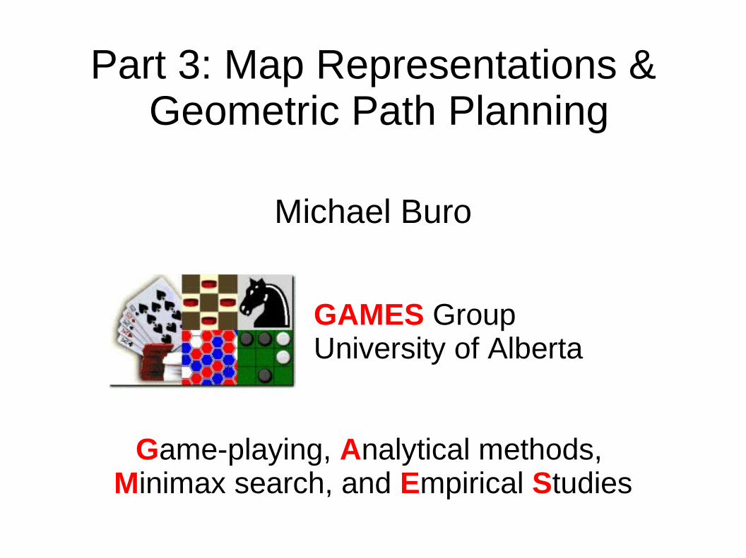
Outline● Map Representations

– Grids, polygon-based

– Free space decompositions

– Constrained Delaunay Triangulations

● Path Planning in Triangulations– A* applied to triangulations (TA*)

– Triangulation Reductions and TRA*

● Outlook– Further improvements

– Applications to high-level game AI

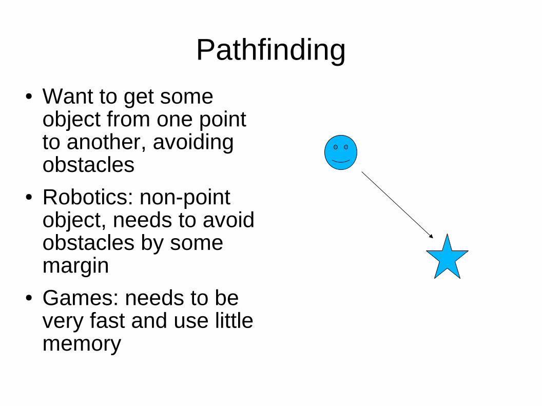
Pathfinding● Want to get some

object from one point to another, avoiding obstacles

● Robotics: non-point object, needs to avoid obstacles by some margin

● Games: needs to be very fast and use little memory

Map Representations● Path planning algorithm is only half the

picture● Underlying map representation and data

structures are just as important● Important design questions:

– Are optimal paths required?– Is the world static or dynamic?– Are worlds known ahead of time?– Are there real-time constraints?– How much memory is available?

Goal of pathfinding algorithms

● Find (nearly) optimal path, where optimal usually means quickest

● Obey constraints (e.g. object size, fuel limit, exposure to enemy fire, real-time)

● Terrain features and some interactions with the environment can be expressed in terms of gaining or losing time– Moving on highways vs. swamps

– Destructible obstacles along the way

● Tradeoff between search space complexity and path quality

State Space Generation

● Worlds can be huge● Like to avoid cumbersome task of picking

waypoints or room abstractions manually● Should be automatically generated from

world geometry

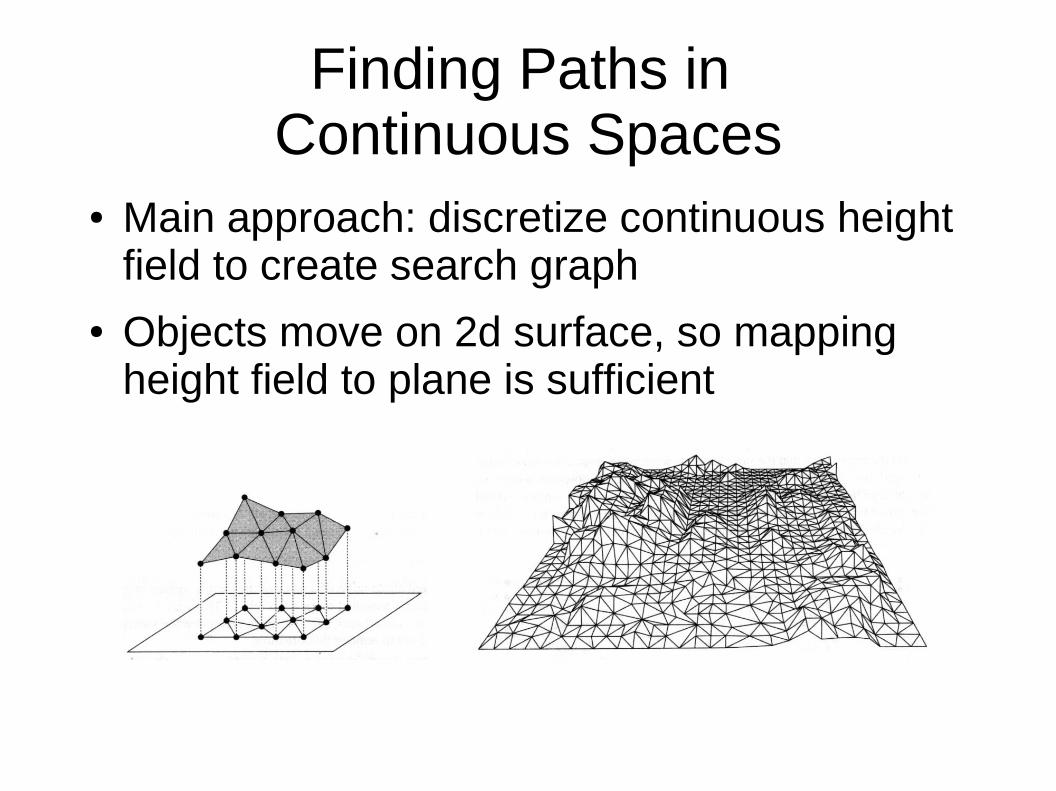
Finding Paths in Continuous Spaces

● Main approach: discretize continuous height field to create search graph

● Objects move on 2d surface, so mapping height field to plane is sufficient

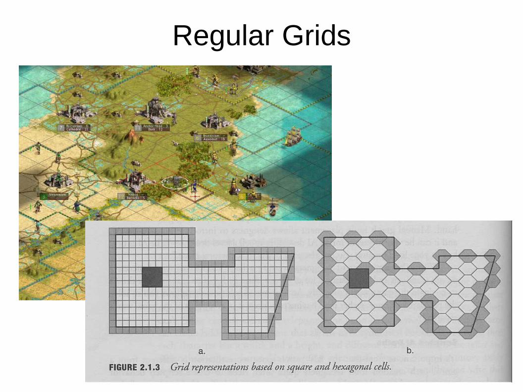
Regular Grids

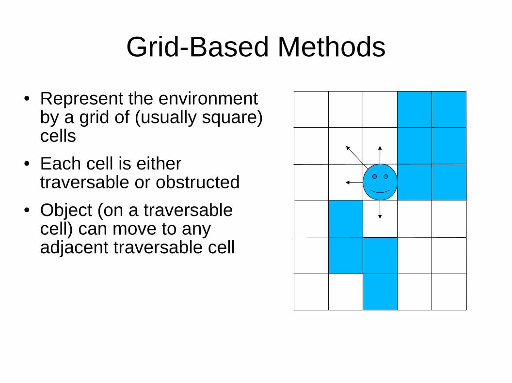
Grid-Based Methods

● Represent the environment by a grid of (usually square) cells

● Each cell is either traversable or obstructed

● Object (on a traversable cell) can move to any adjacent traversable cell

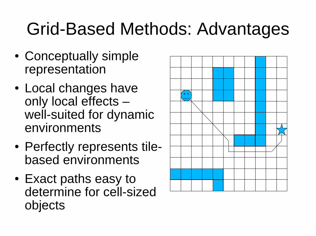
Grid-Based Methods: Advantages● Conceptually simple

representation● Local changes have

only local effects – well-suited for dynamic environments

● Perfectly represents tile-based environments

● Exact paths easy to determine for cell-sized objects

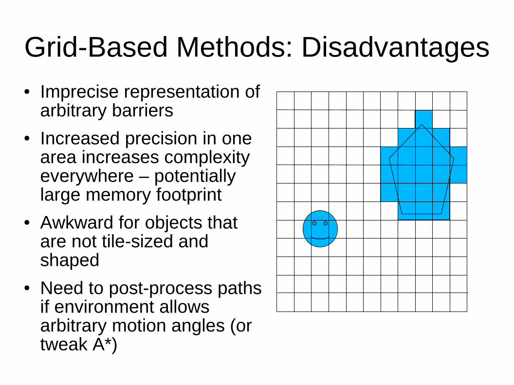
Grid-Based Methods: Disadvantages● Imprecise representation of

arbitrary barriers● Increased precision in one

area increases complexity everywhere – potentially large memory footprint

● Awkward for objects that are not tile-sized and shaped

● Need to post-process paths if environment allows arbitrary motion angles (or tweak A*)

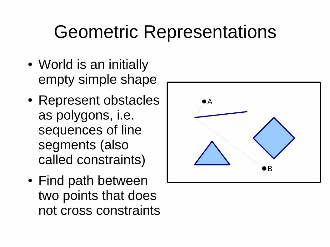
Geometric Representations

● World is an initially empty simple shape

● Represent obstacles as polygons, i.e. sequences of line segments (also called constraints)

● Find path between two points that does not cross constraints

A

B

Geometric Methods

● Advantages– Arbitrary polygon

obstacles

– Arbitrary motion angles

– Memory efficient

– Finding optimal paths for circular objects isn't hard

– Topological abstractions

● Disadvantages– Complex code

– Robustness issues

– Point localization takes more than constant time

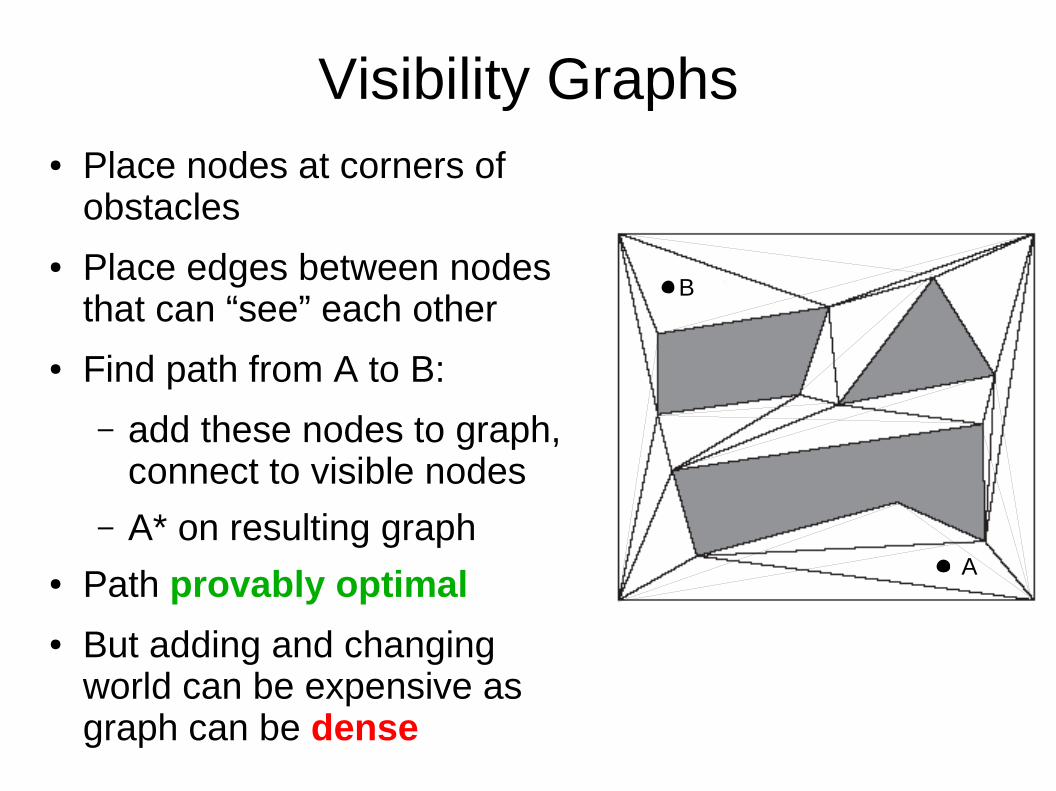
Visibility Graphs● Place nodes at corners of

obstacles

● Place edges between nodes that can “see” each other

● Find path from A to B:

– add these nodes to graph, connect to visible nodes

– A* on resulting graph● Path provably optimal

● But adding and changing world can be expensive as graph can be dense

A

B

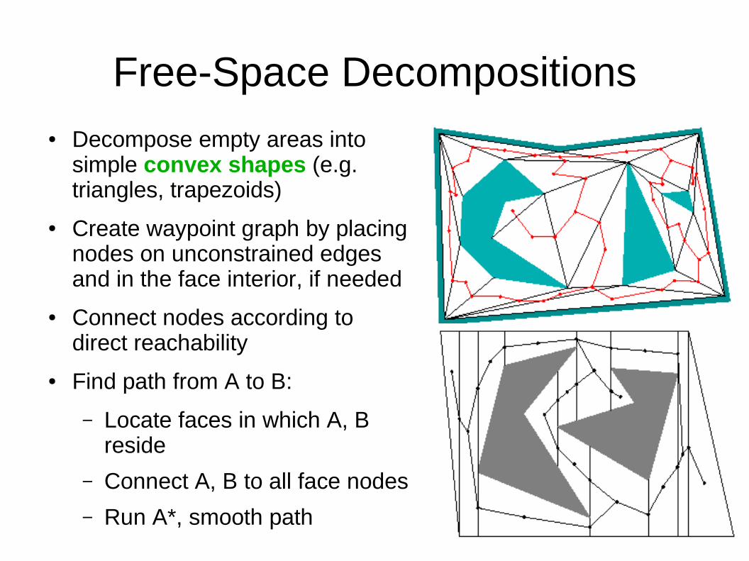
Free-Space Decompositions● Decompose empty areas into

simple convex shapes (e.g. triangles, trapezoids)

● Create waypoint graph by placing nodes on unconstrained edges and in the face interior, if needed

● Connect nodes according to direct reachability

● Find path from A to B:

– Locate faces in which A, B reside

– Connect A, B to all face nodes

– Run A*, smooth path

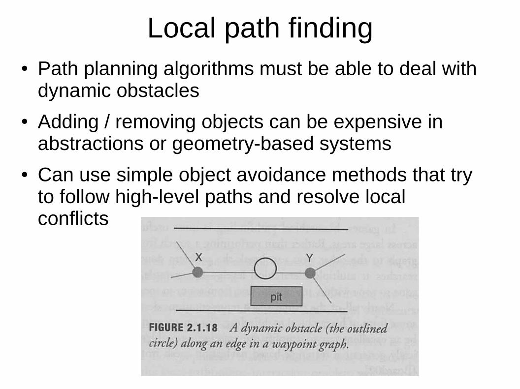
Local path finding● Path planning algorithms must be able to deal with

dynamic obstacles● Adding / removing objects can be expensive in

abstractions or geometry-based systems ● Can use simple object avoidance methods that try

to follow high-level paths and resolve local conflicts

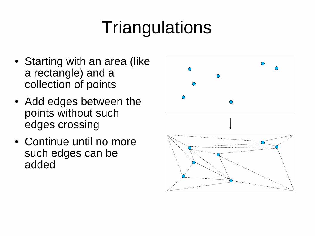
Triangulations

● Starting with an area (like a rectangle) and a collection of points

● Add edges between the points without such edges crossing

● Continue until no more such edges can be added

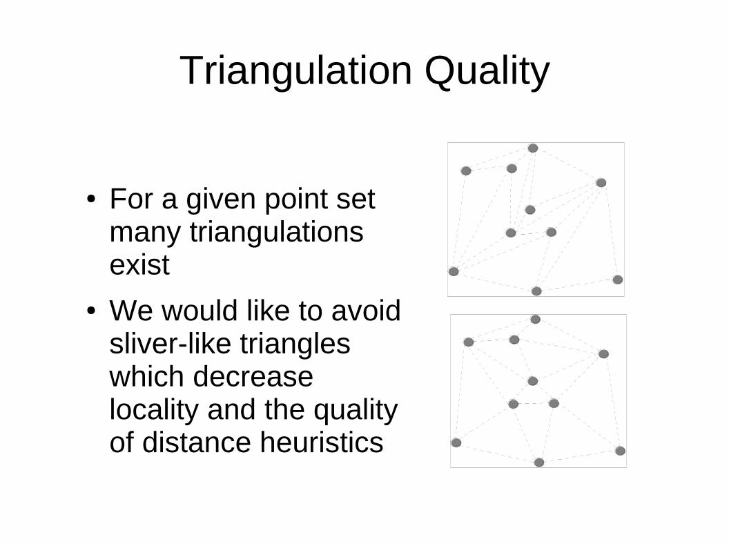
Triangulation Quality

● For a given point set many triangulations exist

● We would like to avoid sliver-like triangles which decrease locality and the quality of distance heuristics

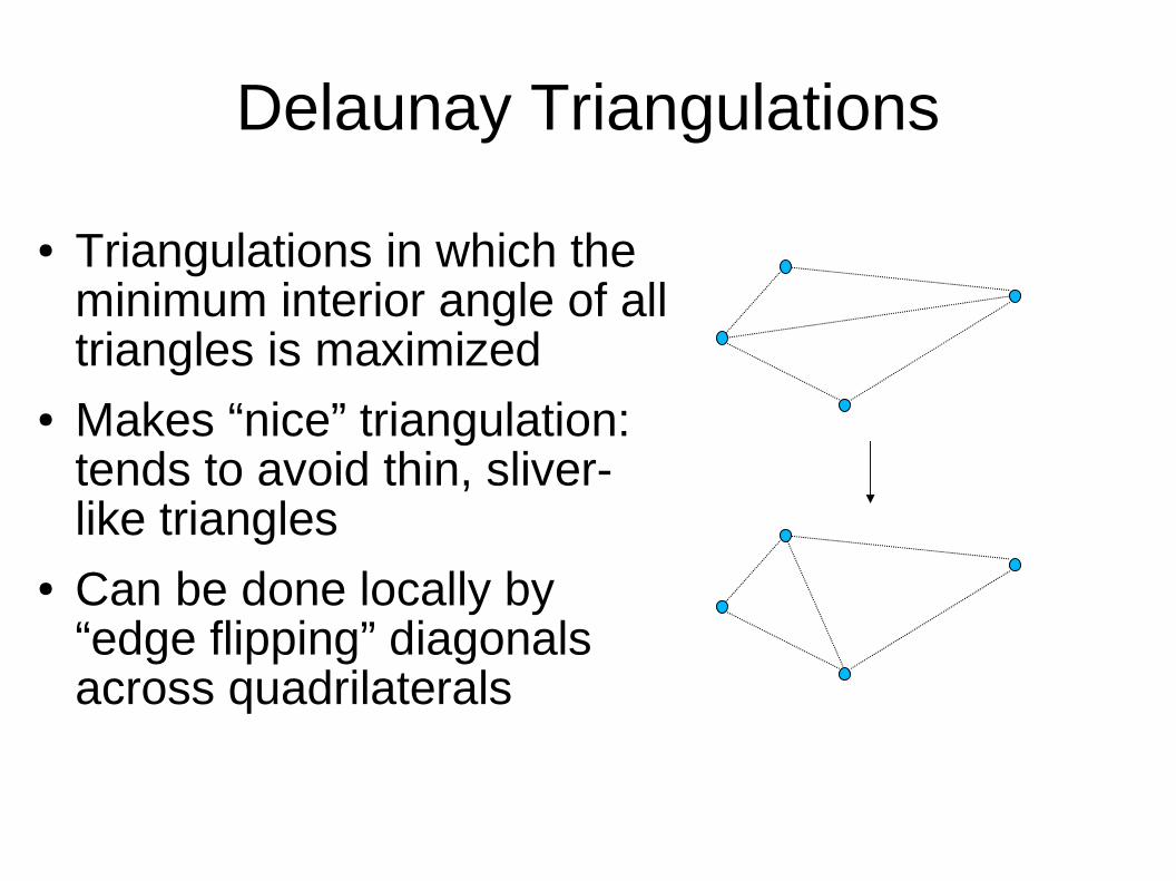
Delaunay Triangulations

● Triangulations in which the minimum interior angle of all triangles is maximized

● Makes “nice” triangulation: tends to avoid thin, sliver-like triangles

● Can be done locally by “edge flipping” diagonals across quadrilaterals

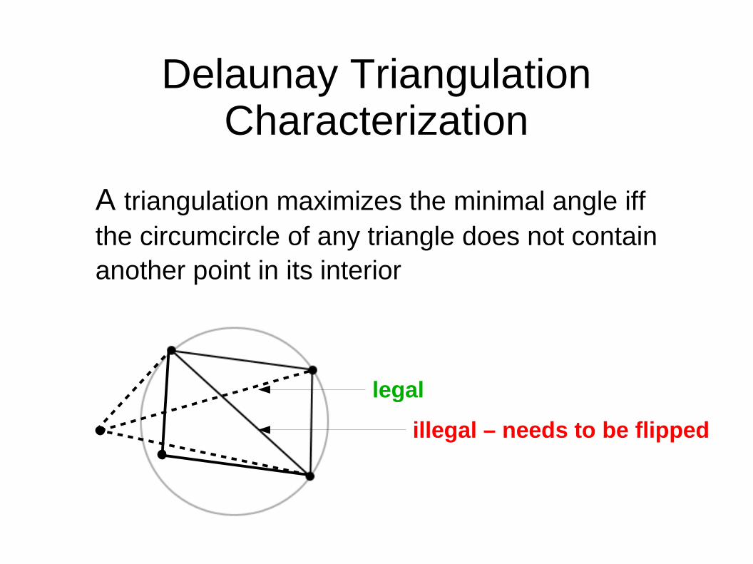
Delaunay Triangulation Characterization

A triangulation maximizes the minimal angle iffthe circumcircle of any triangle does not containanother point in its interior

legal

illegal – needs to be flipped

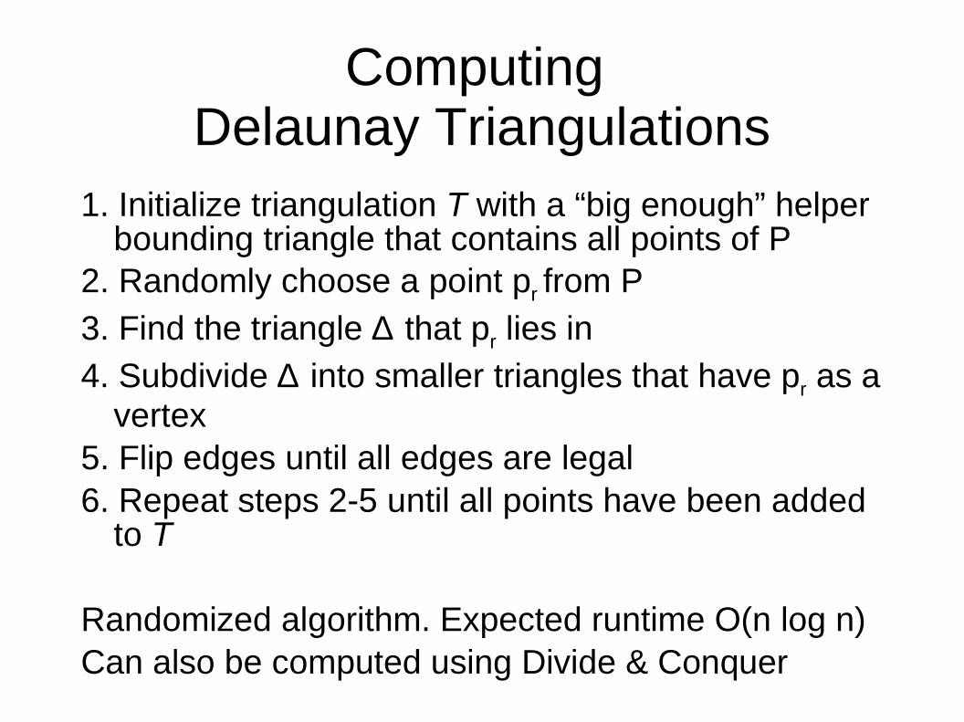
Computing Delaunay Triangulations

1. Initialize triangulation T with a “big enough” helper bounding triangle that contains all points of P

2. Randomly choose a point pr from P

3. Find the triangle ∆ that pr lies in

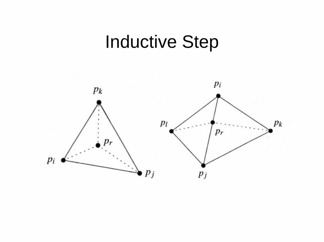
4. Subdivide ∆ into smaller triangles that have pr as a vertex

5. Flip edges until all edges are legal6. Repeat steps 2-5 until all points have been added

to T

Randomized algorithm. Expected runtime O(n log n)Can also be computed using Divide & Conquer

Inductive Step

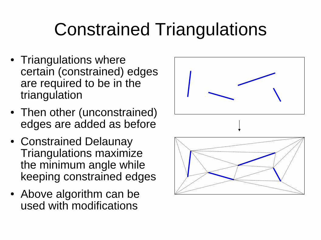
Constrained Triangulations

● Triangulations where certain (constrained) edges are required to be in the triangulation

● Then other (unconstrained) edges are added as before

● Constrained Delaunay Triangulations maximize the minimum angle while keeping constrained edges

● Above algorithm can be used with modifications

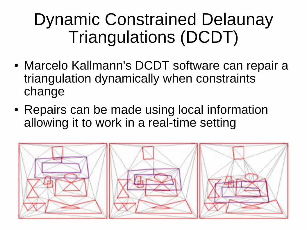
Dynamic Constrained Delaunay Triangulations (DCDT)

● Marcelo Kallmann's DCDT software can repair a triangulation dynamically when constraints change

● Repairs can be made using local information allowing it to work in a real-time setting

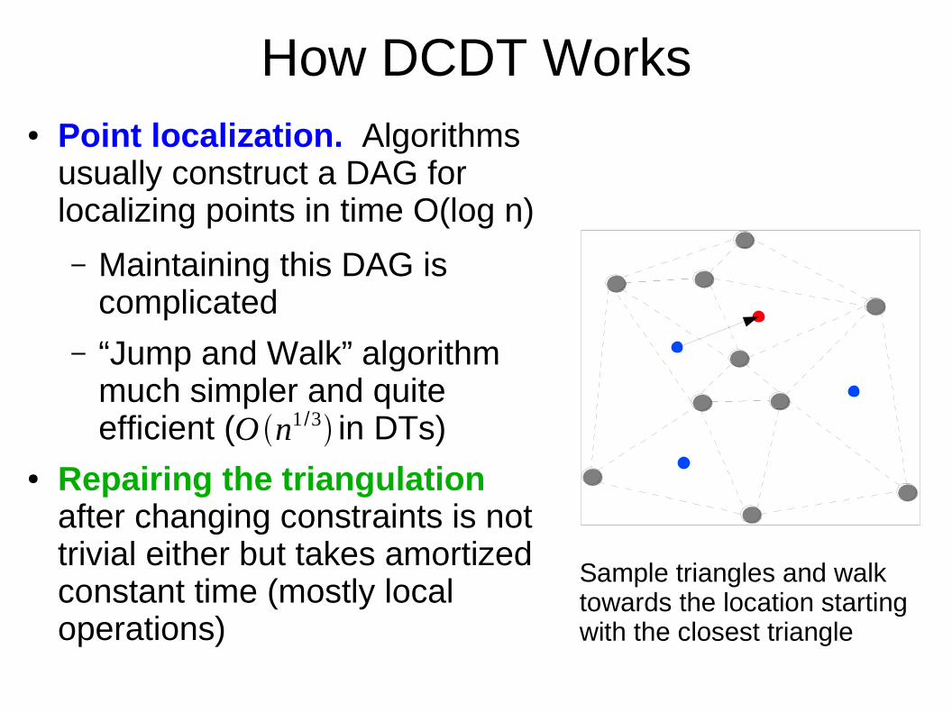
How DCDT Works● Point localization. Algorithms

usually construct a DAG for localizing points in time O(log n)

– Maintaining this DAG is complicated

– “Jump and Walk” algorithm much simpler and quite efficient ( in DTs)

● Repairing the triangulation after changing constraints is not trivial either but takes amortized constant time (mostly local operations)

O n1 /3

Sample triangles and walk towards the location starting with the closest triangle

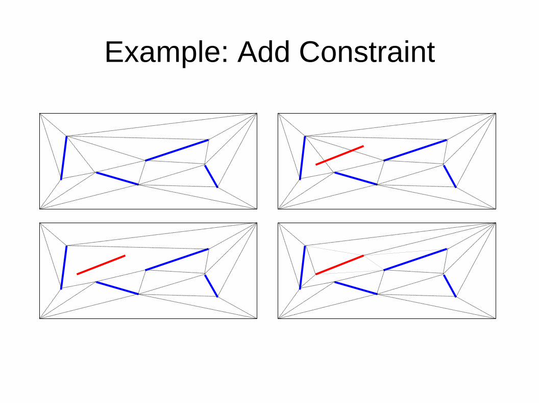
Example: Add Constraint

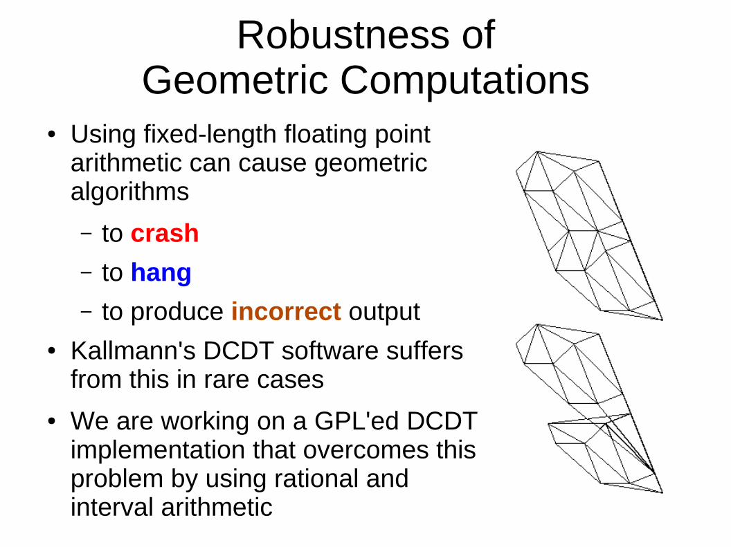
Robustness ofGeometric Computations

● Using fixed-length floating point arithmetic can cause geometric algorithms

– to crash

– to hang

– to produce incorrect output● Kallmann's DCDT software suffers

from this in rare cases

● We are working on a GPL'ed DCDT implementation that overcomes this problem by using rational and interval arithmetic

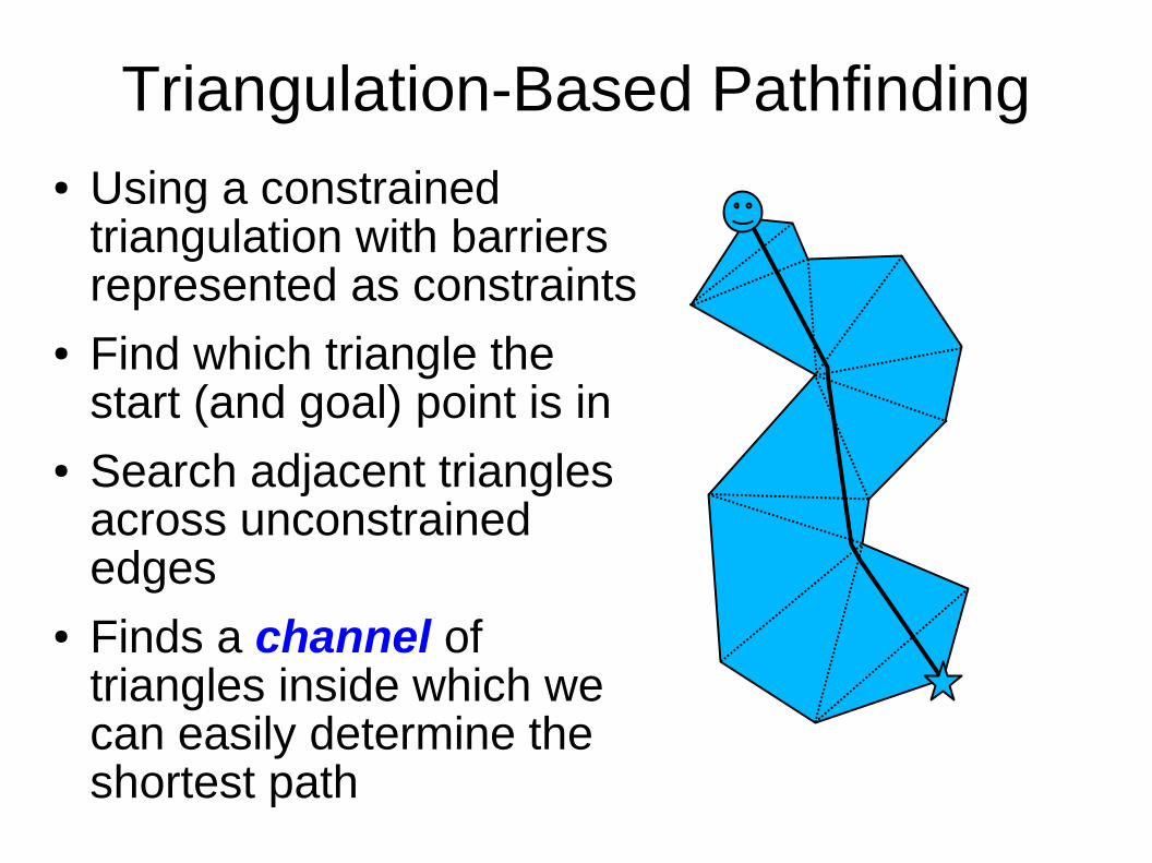
Triangulation-Based Pathfinding● Using a constrained

triangulation with barriers represented as constraints

● Find which triangle the start (and goal) point is in

● Search adjacent triangles across unconstrained edges

● Finds a channel of triangles inside which we can easily determine the shortest path

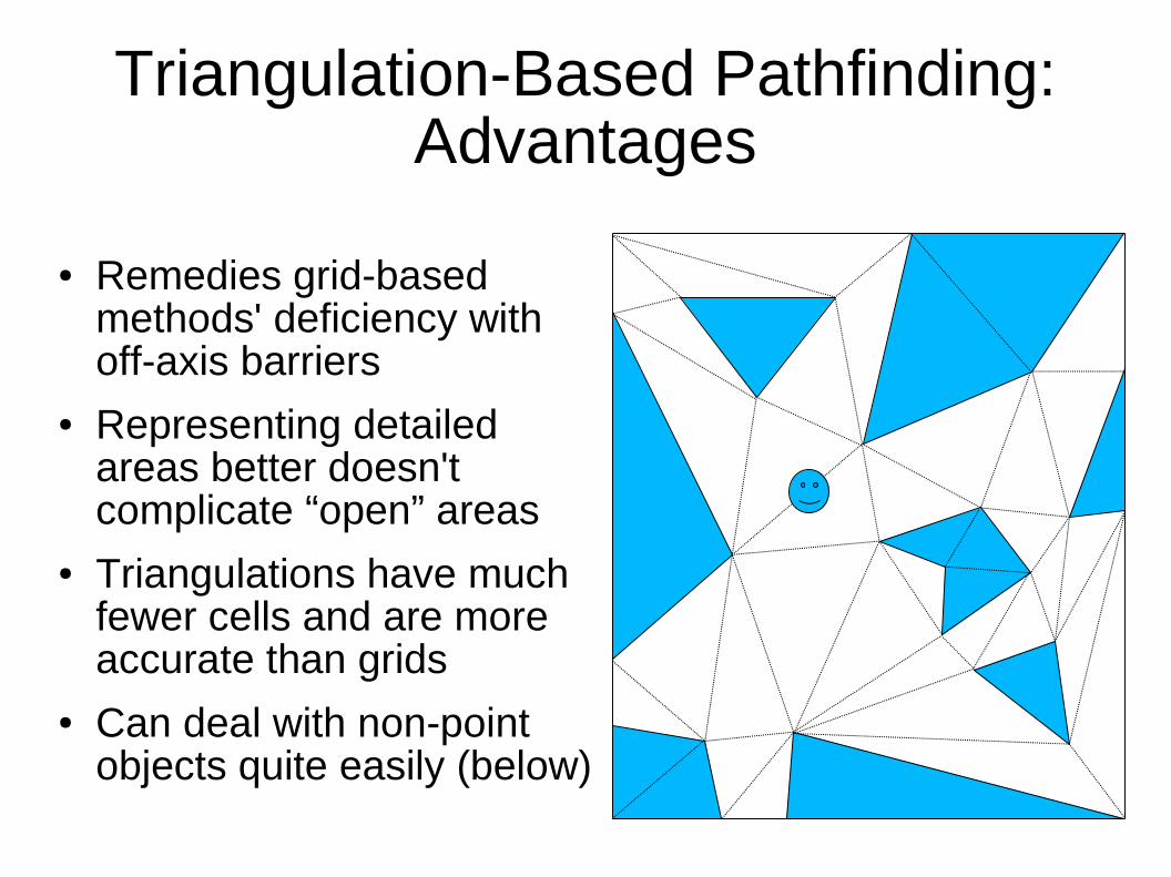
Triangulation-Based Pathfinding:Advantages

● Remedies grid-based methods' deficiency with off-axis barriers

● Representing detailed areas better doesn't complicate “open” areas

● Triangulations have much fewer cells and are more accurate than grids

● Can deal with non-point objects quite easily (below)

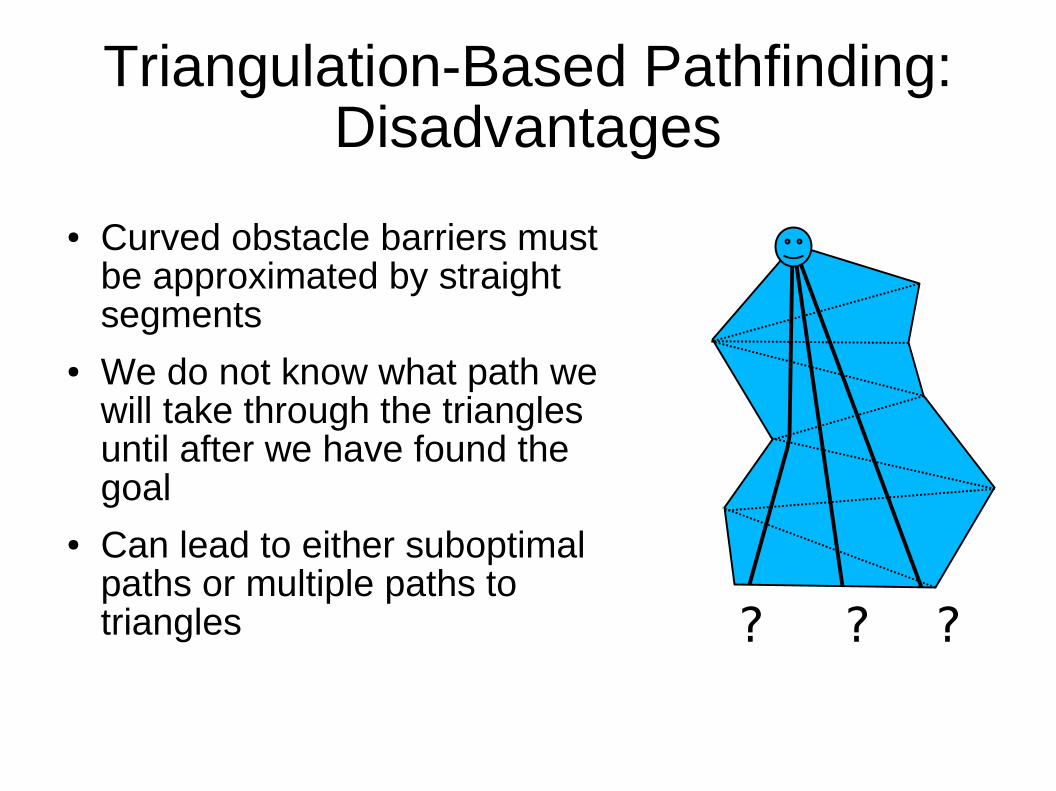
Triangulation-Based Pathfinding: Disadvantages

● Curved obstacle barriers must be approximated by straight segments

● We do not know what path we will take through the triangles until after we have found the goal

● Can lead to either suboptimal paths or multiple paths to triangles ? ? ?

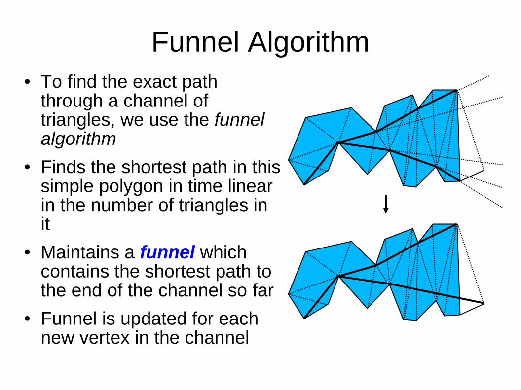
Funnel Algorithm● To find the exact path

through a channel of triangles, we use the funnel algorithm

● Finds the shortest path in this simple polygon in time linear in the number of triangles in it

● Maintains a funnel which contains the shortest path to the end of the channel so far

● Funnel is updated for each new vertex in the channel

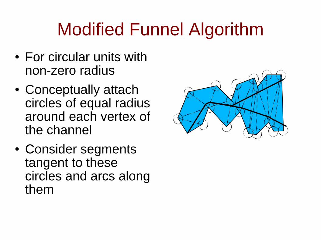
Modified Funnel Algorithm● For circular units with

non-zero radius● Conceptually attach

circles of equal radius around each vertex of the channel

● Consider segments tangent to these circles and arcs along them

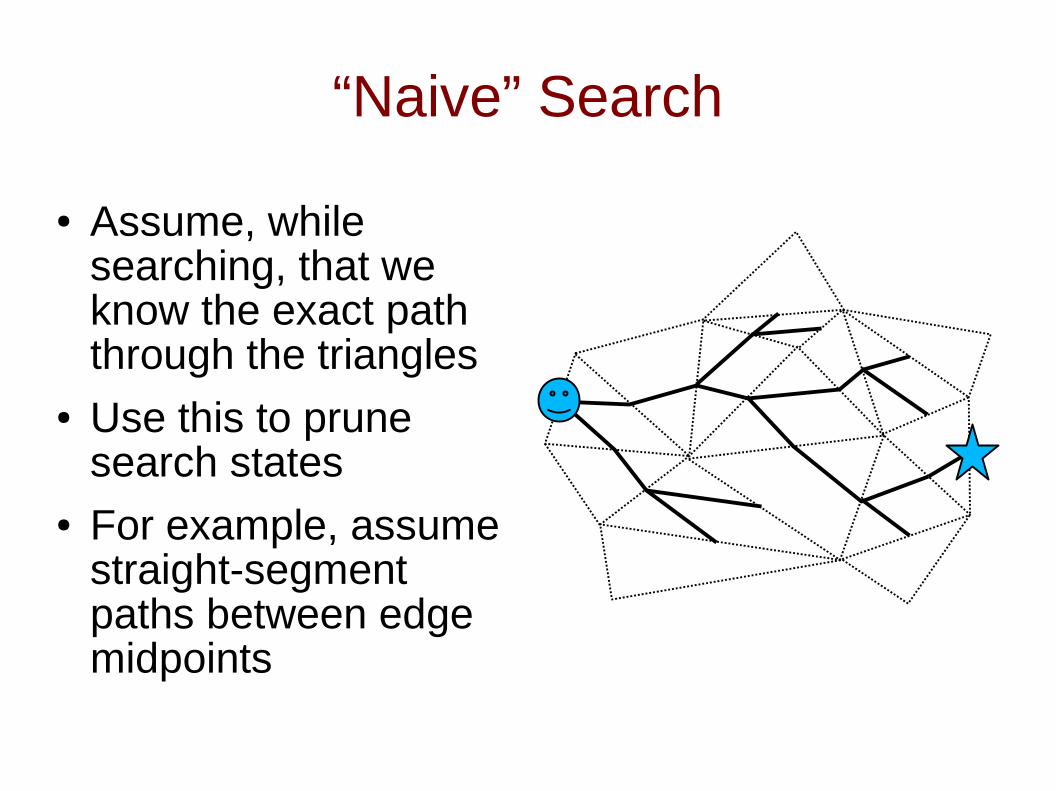
“Naive” Search

● Assume, while searching, that we know the exact path through the triangles

● Use this to prune search states

● For example, assume straight-segment paths between edge midpoints

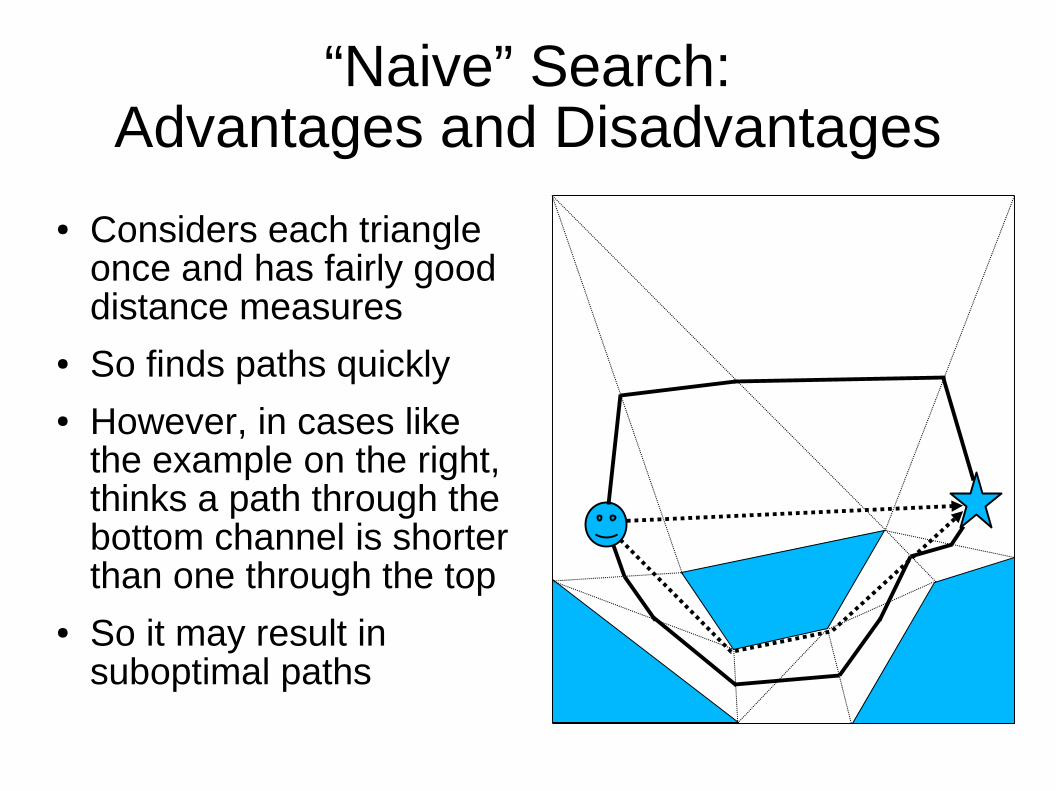
“Naive” Search:Advantages and Disadvantages

● Considers each triangle once and has fairly good distance measures

● So finds paths quickly● However, in cases like

the example on the right, thinks a path through the bottom channel is shorter than one through the top

● So it may result in suboptimal paths

How To Find Optimal Paths?● (Under)estimate the distance travelled so far● Allow multiple paths to any triangle● When a channel is found to the goal, calculate

the length of the shortest path in this channel● If it is the shortest path found so far, keep it,

otherwise, reject it (anytime algorithm)● When the distance travelled so far for the paths

yet to be searched exceeds the length of the shortest path, the algorithm ends and we have an optimal path

Triangulation A* (TA*)● Search running on the base triangulation● Uses a triangle for a search state and the adjacent

triangles across unconstrained edges as neighbors● Using anytime algorithm and considering multiple

paths to a triangle as described earlier● For a heuristic (h-value), take the Euclidean

distance between the goal and any point on the triangle's entry edge

● Calculate an underestimate for the distance-travelled-so-far (g-value)

● Only considers triangles once until the first path is found

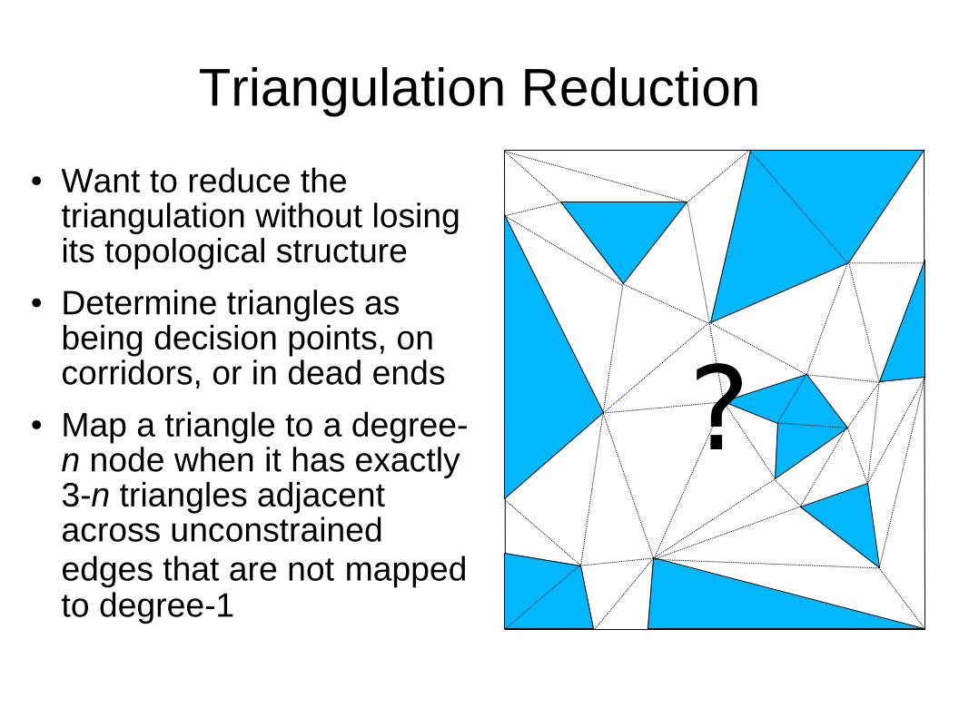
Triangulation Reduction

● Want to reduce the triangulation without losing its topological structure

● Determine triangles as being decision points, on corridors, or in dead ends

● Map a triangle to a degree-n node when it has exactly 3-n triangles adjacent across unconstrained edges that are not mapped to degree-1

?

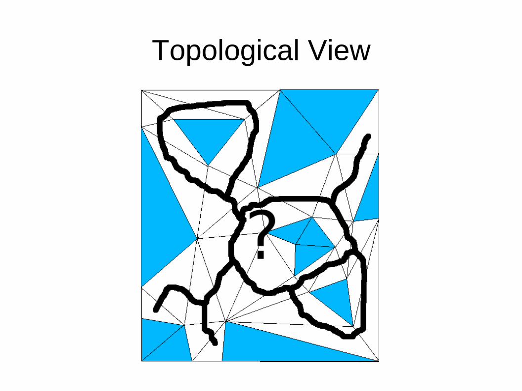
Topological View

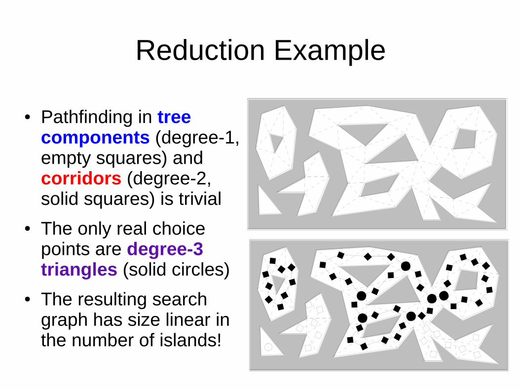
Reduction Example

● Pathfinding in tree components (degree-1, empty squares) and corridors (degree-2, solid squares) is trivial

● The only real choice points are degree-3 triangles (solid circles)

● The resulting search graph has size linear in the number of islands!

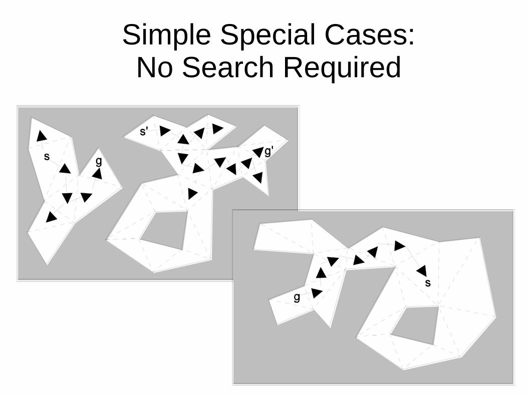
Simple Special Cases: No Search Required

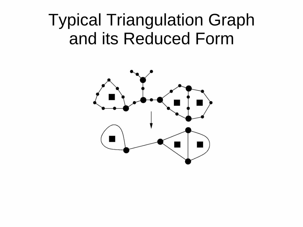
Typical Triangulation Graphand its Reduced Form

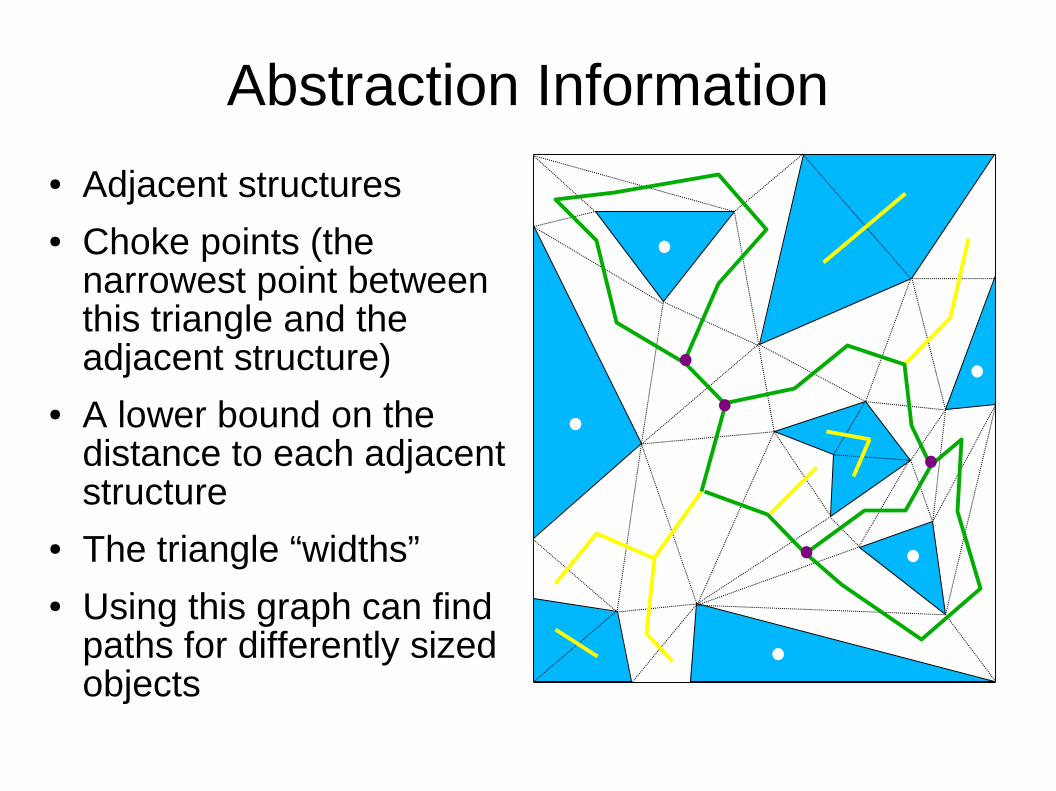
Abstraction Information

● Adjacent structures● Choke points (the

narrowest point between this triangle and the adjacent structure)

● A lower bound on the distance to each adjacent structure

● The triangle “widths”● Using this graph can find

paths for differently sized objects

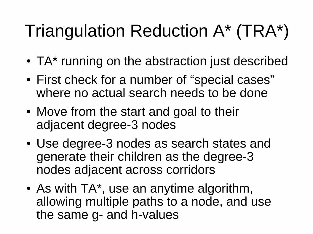
Triangulation Reduction A* (TRA*)

● TA* running on the abstraction just described● First check for a number of “special cases”

where no actual search needs to be done● Move from the start and goal to their

adjacent degree-3 nodes● Use degree-3 nodes as search states and

generate their children as the degree-3 nodes adjacent across corridors

● As with TA*, use an anytime algorithm, allowing multiple paths to a node, and use the same g- and h-values

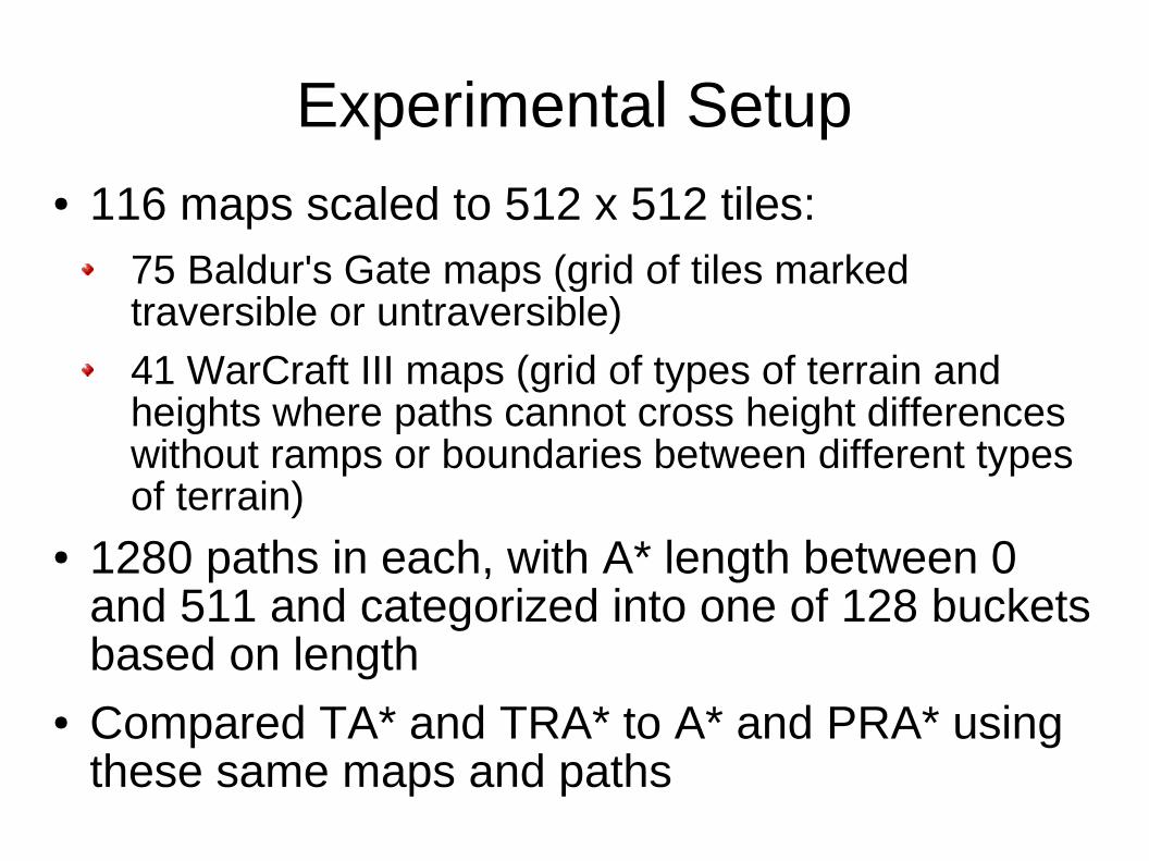
Experimental Setup● 116 maps scaled to 512 x 512 tiles:

75 Baldur's Gate maps (grid of tiles marked traversible or untraversible)

41 WarCraft III maps (grid of types of terrain and heights where paths cannot cross height differences without ramps or boundaries between different types of terrain)

● 1280 paths in each, with A* length between 0 and 511 and categorized into one of 128 buckets based on length

● Compared TA* and TRA* to A* and PRA* using these same maps and paths

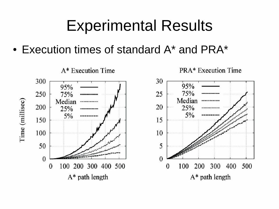
Experimental Results● Execution times of standard A* and PRA*

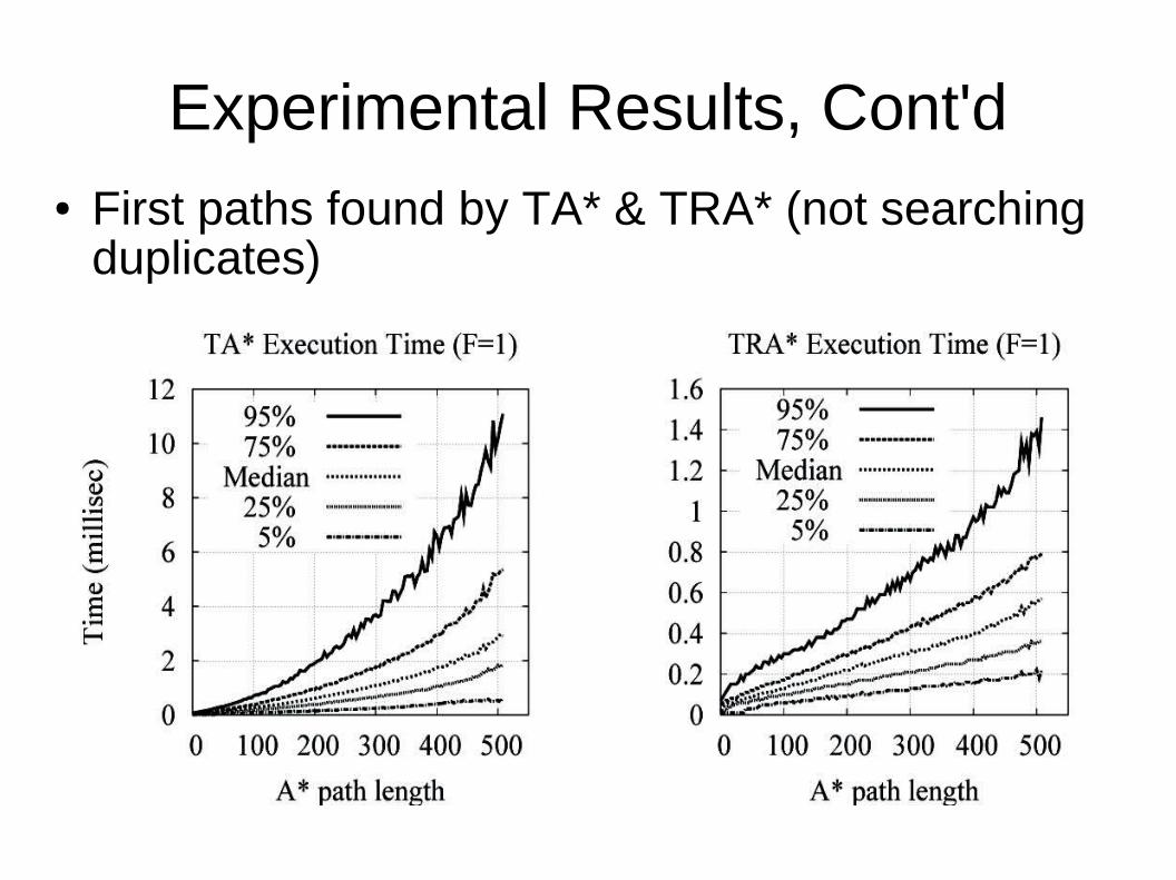
Experimental Results, Cont'd● First paths found by TA* & TRA* (not searching

duplicates)

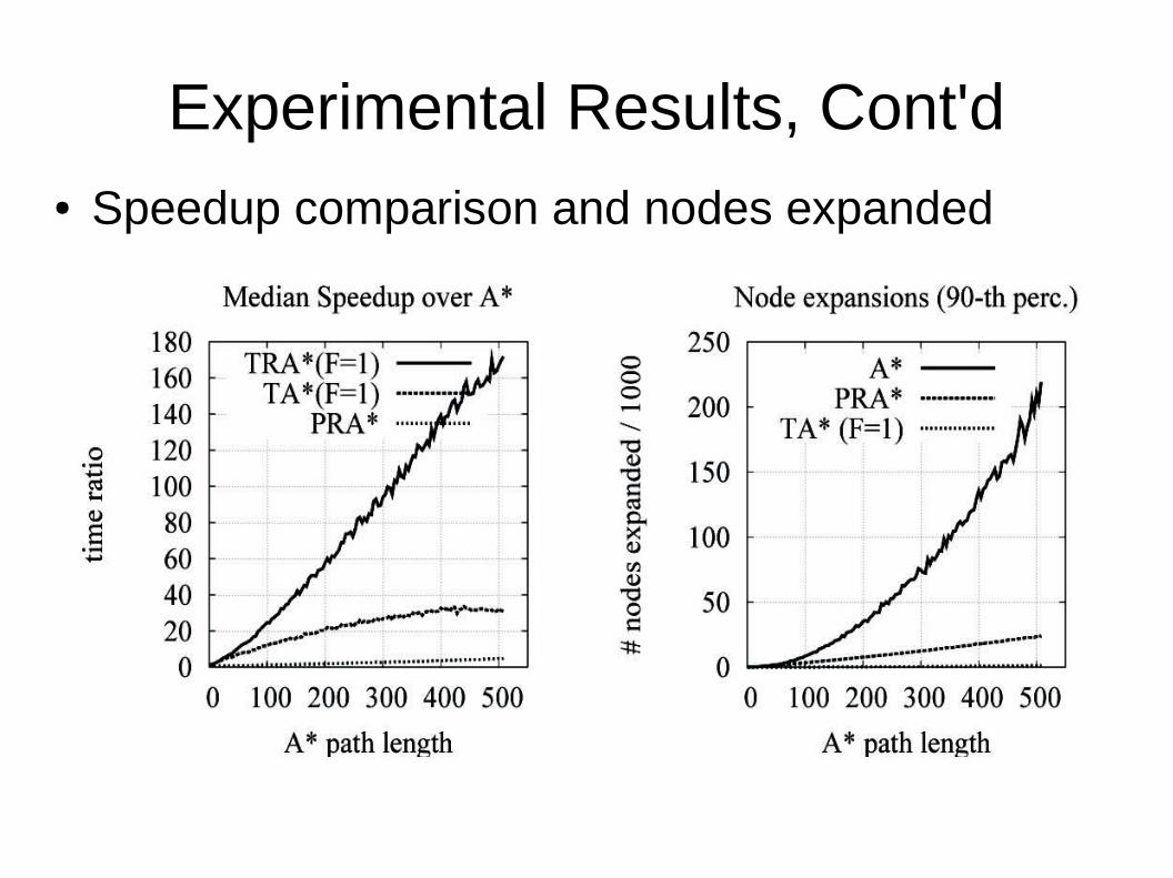
Experimental Results, Cont'd● Speedup comparison and nodes expanded

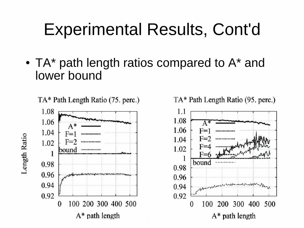
Experimental Results, Cont'd

● TA* path length ratios compared to A* and lower bound

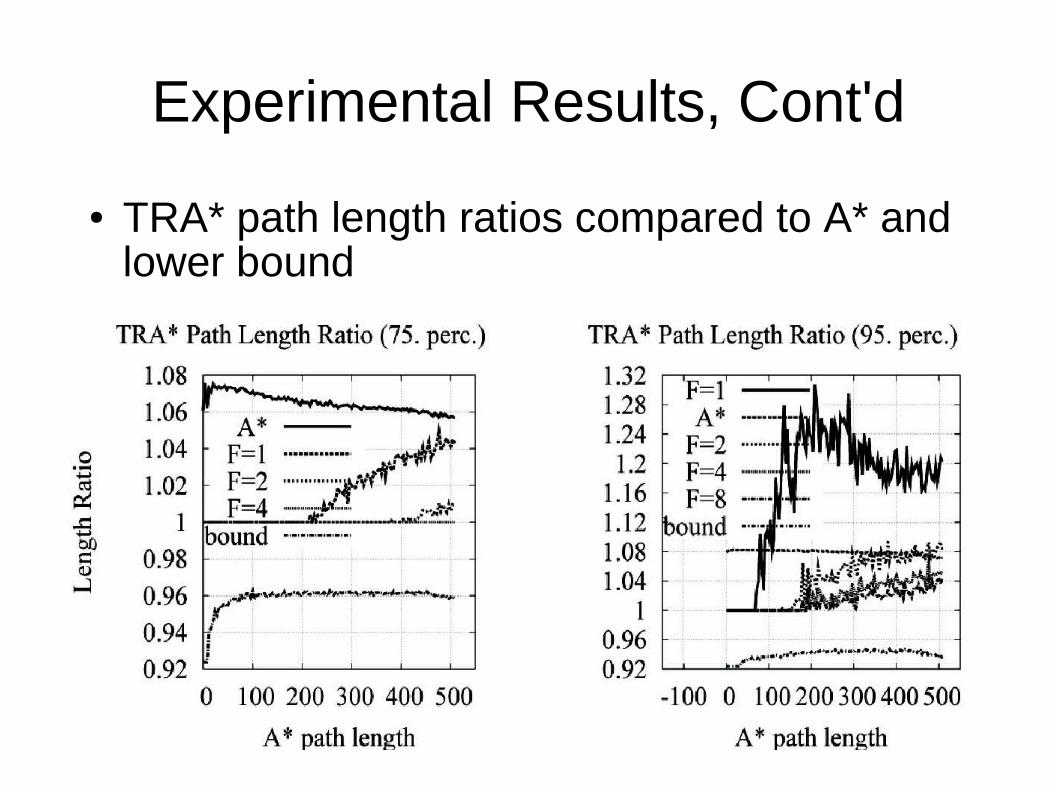
Experimental Results, Cont'd

● TRA* path length ratios compared to A* and lower bound

Conclusions

● Triangulations can accurately and efficiently represent polygonal environments

● Triangulations offer unique possibilities for pathfinding for a non-point (especially circular) object

● Triangulation-based pathfinding finds paths very quickly and can also find optimal paths given a bit more time

● Our abstraction technique identifies useful structures in the environment: dead-ends, corridors, and decision points

● This abstraction can be used to find paths even more quickly, only depending on the number of obstacles

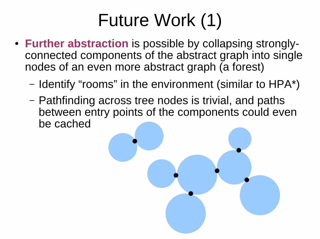
Future Work (1)● Further abstraction is possible by collapsing strongly-

connected components of the abstract graph into single nodes of an even more abstract graph (a forest)

– Identify “rooms” in the environment (similar to HPA*)– Pathfinding across tree nodes is trivial, and paths

between entry points of the components could even be cached

Future Work (2)● Channels resulting from TA* or TRA* are

useful in pathfinding involving multiple objects because channel widths are known

● Terrain analysis is possible with the abstraction information (e.g. identifying choke points)

● More edge annotations can reduce the need for triangulation updates (e.g. enemy presense in corridors)

● It may be useful to construct waypoint graphs from triangulations that produce close to optimal paths in one shot

References● AI Game Programming Wisdom Book Series● M. de Berg et al., Computational Geometry, 3rd

edition, Springer Verlag 2008● M. Kallmann, H. Bieri, D. Thalmann, Fully

Dynamic Constraint Delaunay Triangulations, in Geometric Modeling for Scientific Visualization, Springer Verlag 2003

● M. Kallmann, Pathplanning in Triangulations, IJCAI 2005

● D. Demyen, Triangulation-Based Pathfinding, MSc. Thesis, 2006, which is summarized in:

● D. Demyen and M. Buro, Efficient Triangulation-Based Pathfinding, AAAI 2006

Extra Material

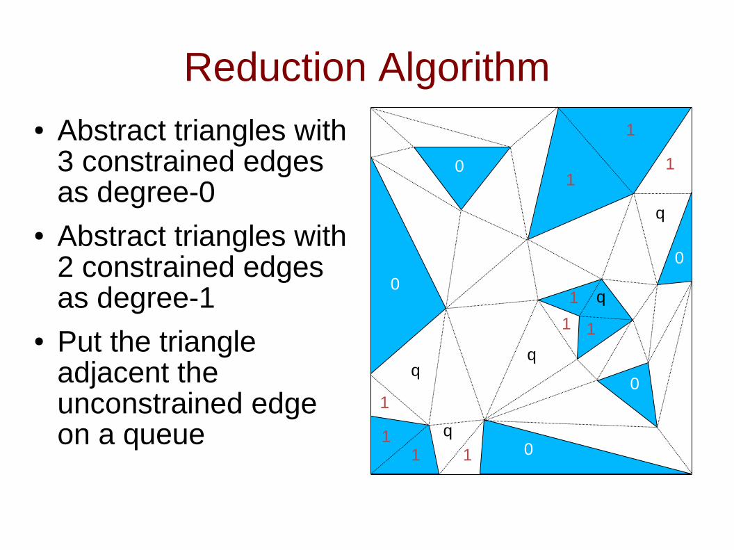
Reduction Algorithm● Abstract triangles with

3 constrained edges as degree-0

● Abstract triangles with 2 constrained edges as degree-1

● Put the triangle adjacent the unconstrained edge on a queue

1

1

11

11

1

1

1

1

q

q

q

q

0

0

0

0

0

q

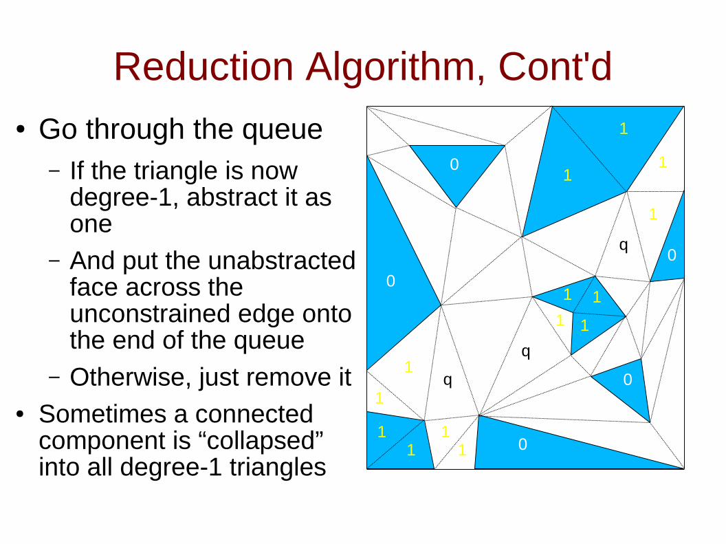
Reduction Algorithm, Cont'd● Go through the queue

– If the triangle is now degree-1, abstract it as one

– And put the unabstracted face across the unconstrained edge onto the end of the queue

– Otherwise, just remove it● Sometimes a connected

component is “collapsed” into all degree-1 triangles

1

1

11

11

1

1

1

1

q

q

0

0

0

0

0

1

1

1

1

q

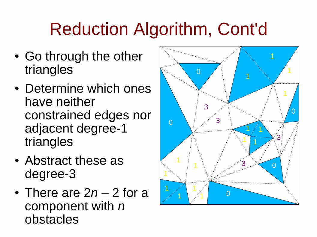
Reduction Algorithm, Cont'd● Go through the other

triangles● Determine which ones

have neither constrained edges nor adjacent degree-1 triangles

● Abstract these as degree-3

● There are 2n – 2 for a component with n obstacles

1

1

11

11

1

1

1

1

0

0

0

0

0

1

1

1

1

1

3

3

3

3

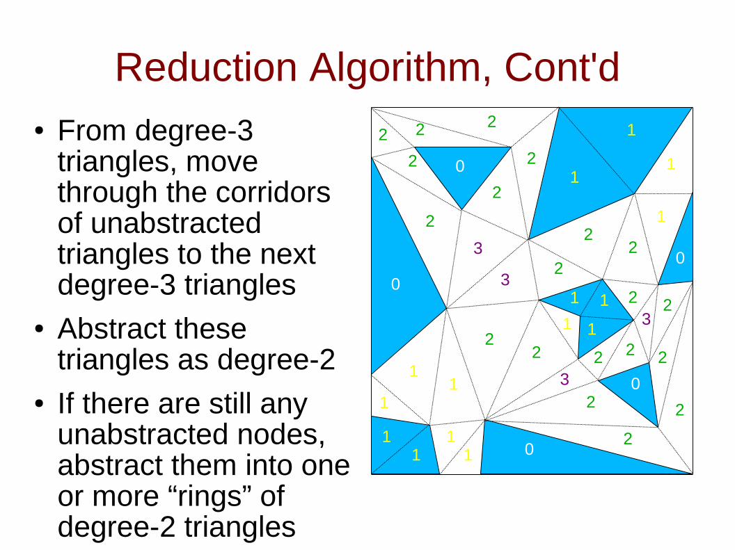
Reduction Algorithm, Cont'd● From degree-3

triangles, move through the corridors of unabstracted triangles to the next degree-3 triangles

● Abstract these triangles as degree-2

● If there are still any unabstracted nodes, abstract them into one or more “rings” of degree-2 triangles

1

1

11

11

1

1

1

1

0

0

0

0

0

1

1

1

1

1

3

3

3

3

2 2 2

22

2

2

2

2

22

2 2 2

2

2

2

2

2

2

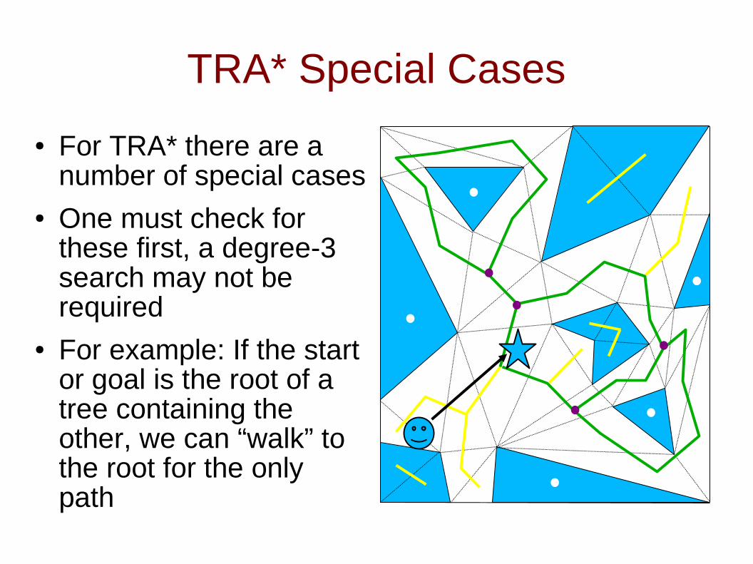
TRA* Special Cases

● For TRA* there are a number of special cases

● One must check for these first, a degree-3 search may not be required

● For example: If the start or goal is the root of a tree containing the other, we can “walk” to the root for the only path

TRA* Special Cases, Cont'd

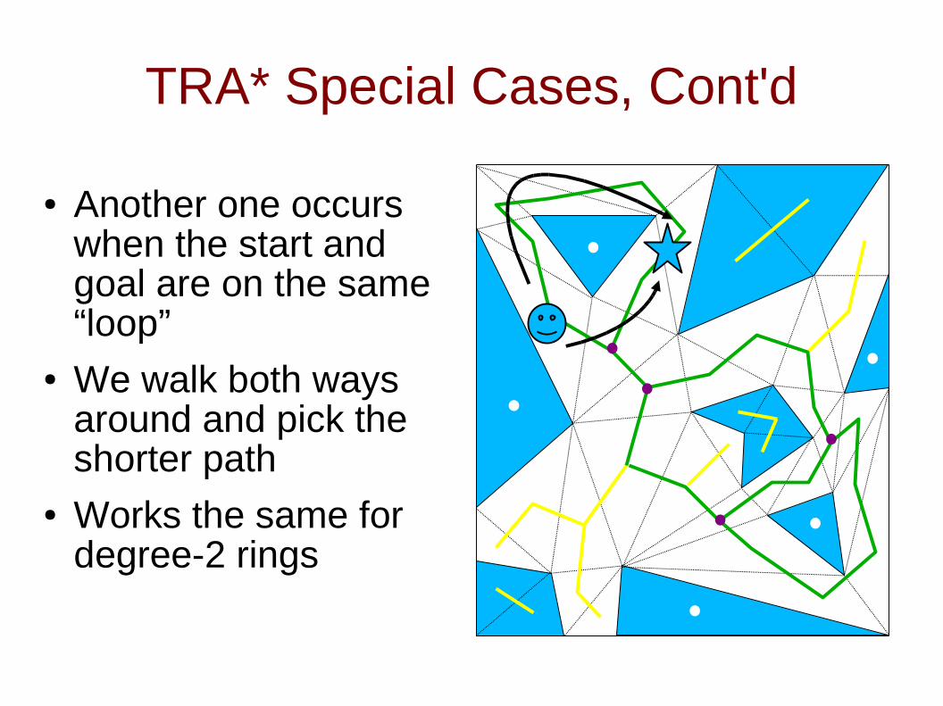
● Another one occurs when the start and goal are on the same “loop”

● We walk both ways around and pick the shorter path

● Works the same for degree-2 rings

TRA* Special Cases, Cont'd

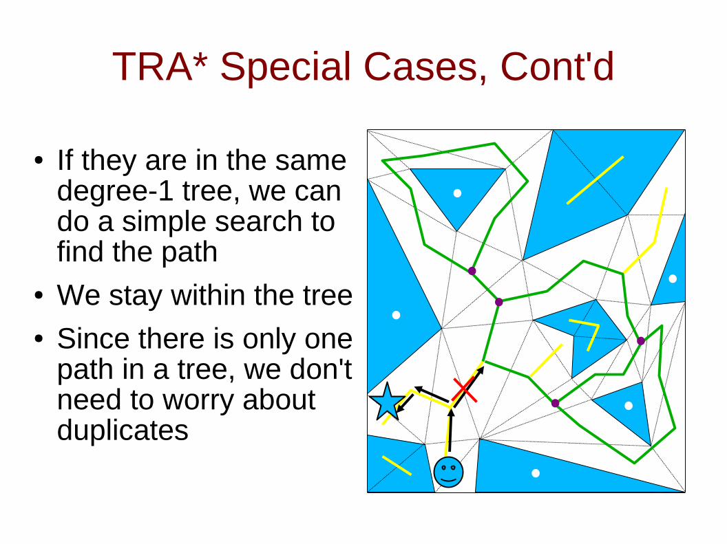
● If they are in the same degree-1 tree, we can do a simple search to find the path

● We stay within the tree● Since there is only one

path in a tree, we don't need to worry about duplicates

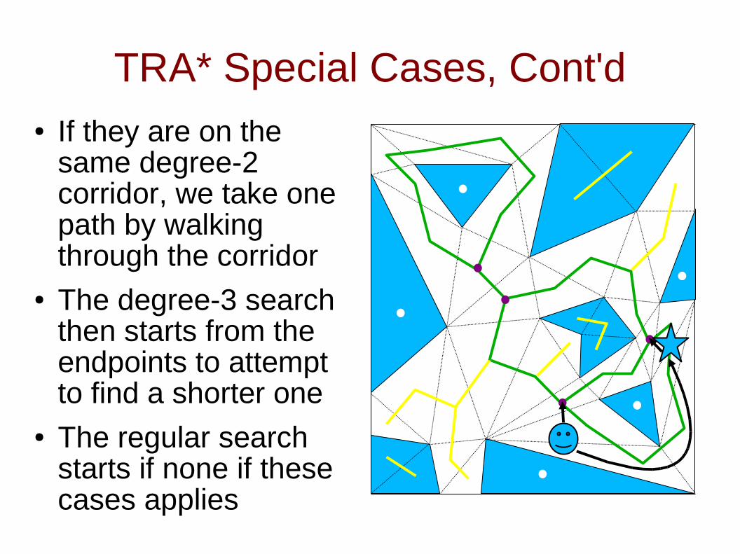
TRA* Special Cases, Cont'd● If they are on the

same degree-2 corridor, we take one path by walking through the corridor

● The degree-3 search then starts from the endpoints to attempt to find a shorter one

● The regular search starts if none if these cases applies

TRA* Degree-3 Node Search

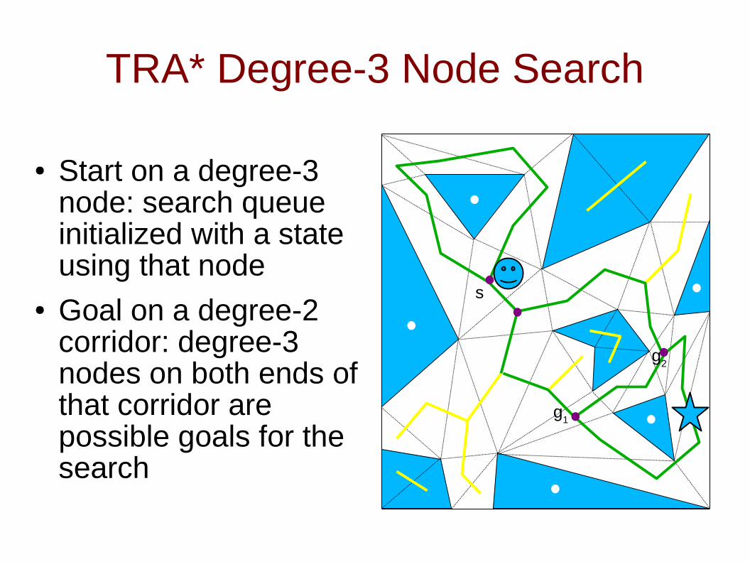
● Start on a degree-3 node: search queue initialized with a state using that node

● Goal on a degree-2 corridor: degree-3 nodes on both ends of that corridor are possible goals for the search

s

g1

g2

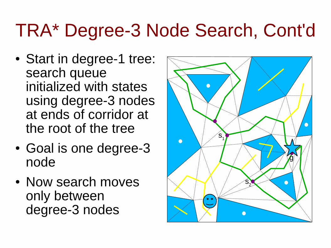
TRA* Degree-3 Node Search, Cont'd● Start in degree-1 tree:

search queue initialized with states using degree-3 nodes at ends of corridor at the root of the tree

● Goal is one degree-3 node

● Now search moves only between degree-3 nodes

g

s1

s2