Embed Size (px)
Citation preview

Outline Introduction Digital image Histogram Contrast Equalisation
Part 3: Image ProcessingDigital Images and Intensity Histograms
Georgy Gimel’farb
COMPSCI 373 Computer Graphics and Image Processing
1 / 47

Outline Introduction Digital image Histogram Contrast Equalisation
1 Introduction
2 Digital image
3 Image histogram
4 Image contrast
5 Histogram equalisation
2 / 47

Outline Introduction Digital image Histogram Contrast Equalisation
• Lecturer: Georgy Gimel’farb (georgy@cs; 86609)
• Office hours: whenever the door of 303S.389 is open. . .
Part 3 overview:
1 Digital images and intensity histograms
2 Basics of binary and greyscale mathematical morphology
3 Image filtering and segmentation
4 Filtering revisited: Moving Window Transform
MRI segmentation=⇒
3 / 47

Outline Introduction Digital image Histogram Contrast Equalisation
Digital Images in Computer Vision and Graphics
Examples of the combined use of image processing, computervision, and computer graphics techniques
Reconstructing a three-dimensional(3D) depth map from a stereo pair of2D images.
Reconstructed animated 4D (3D +time) face model.
4 / 47

Outline Introduction Digital image Histogram Contrast Equalisation
Digital Images in Computer Vision and Graphics
Examples of the combined use of image processing, computervision, and computer graphics techniques
Reconstructing a 3D depth map from a stereo pair.
5 / 47
Outline Introduction Digital image Histogram Contrast Equalisation
Digital Images in Computer Vision and Graphics
Examples of the combined use of image processing, computervision, and computer graphics techniques
Animated 4D viewing of reconstructed 3D trees.
6 / 47

Outline Introduction Digital image Histogram Contrast Equalisation
What to Do with Digital Images?
• Image Processing: transform one or more images into newimage(s).
• Computer Vision: analyze one or more images to getinformation about what is depicted in the image(s).
• Computer Graphics: generate images from descriptions ofwhat should be depicted.
IN
PU
T
O U T P U TDescriptions Images
Descriptions Text Processing Computer GraphicsImages Computer Vision: Image Processing:
• Intensity histogram
• Image segmentation
• Erosion, dilation
• Opening, closing
7 / 47
Outline Introduction Digital image Histogram Contrast Equalisation
Pixels and Image Resolution
Pixel (picture cell) or pel (picture element)
Position (x, y) + greyscale (intensity) or colour signal value v
Origin (0, 0) of pixel coordinates is sometimes in top left corner.
• Resolution: how many pixels? [width × height]• Warning on origin and axes:
• Origin may be sometimes at top left corner with y-axispointing downwards.
• Some software (Matlab) may not accept 0 as a valid index.
8 / 47
Outline Introduction Digital image Histogram Contrast Equalisation
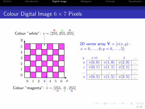
Colour Digital Image 6× 7 Pixels
y
x0 1 2 3 4 5 6
0
1
2
3
4
5
Colour ”white”: v = [R
255,G
255,B
255]
Colour ”magenta”: v = [255R, 0
G, 255
B]
2D vector array V = [v(x, y) :x = 0, . . . , 6; y = 0, . . . , 5]:
y x=0 1 2 ...
0 v(0, 0) v(1, 0) v(2, 0) ...
1 v(0, 1) v(1, 1) v(2, 1) ...
... ... ... ... ...
5 v(0, 5) v(1, 5) v(2, 5) ...
9 / 47

Outline Introduction Digital image Histogram Contrast Equalisation
Encoding of Colours
Bit depth: a number of bits used to represent eachpixel’s value (typically 1, 8, 24, or 32).
• Binary image (1 bit / pixel).• Only two codes – 0 (black) and 1 (white).
• Scalar/monochrome/greyscale image (8 bits).• Scalar codes: just a single number per colour.• No colour – grey values from black to white.
• Vector-valued image: vector codes (≥ 24 bits).• Several (e.g. three) numbers per colour.• All the colors can be represented
This course considers mostly binary and greyscaleimages only.
10 / 47

Outline Introduction Digital image Histogram Contrast Equalisation
Defining Images Mathematically
An image can be defined on an M ×N arithmetic grid, or lattice:RM,N = {(x, y) : x = 1, 2, . . . ,M ; y = 1, 2, . . . , N}
• (x, y) – pixel coordinates.
• An image as a graph of afunction f : R→ V.
• V – a set of signal values,e.g. grey levels or colours.
• Example: pixel at position(100, 50) has scalar value255, i.e. f(100, 50) = 255.
x
y
1 2 3 4 5 6 M
1
2
3
4
5
N
11 / 47
Outline Introduction Digital image Histogram Contrast Equalisation
Image Histogram
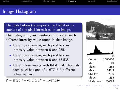
The distribution (or empirical probabilities, orcounts) of the pixel intensities in an image.
The histogram gives numbers of pixels at eachdifferent intensity value found in that image.
• For an 8-bit image, each pixel has anintensity value between 0 and 255.
• For a 16-bit image, each pixel has anintensity value between 0 and 65,535.
• For a colour image with 8-bit RGB channels,each pixel has one of 1, 677, 216 differentcolour values.
28 = 256; 216 = 65, 536; 224 = 1, 677, 216
Count: 1080000Min: 10Max: 255Mean: 146.9StdDev: 73.6Mode: 255Mode count: 236885
12 / 47

Outline Introduction Digital image Histogram Contrast Equalisation
Image Histogram
• An M ×N greyscale 8-bit image v (M rowsand N columns) has K =M ×N pixels.
• Each pixel (x, y) has an integer intensityv(x, y) in the range Q = [0, 1, . . . , 255].
The histogram H : Q→ [0, 1, . . . ,K] for theimage v records the numbers, H(q), of pixelswith intensities v(x, y) = q ∈ Q:
H(q) =(M,N)∑
(x,y)=(0,0)
δ(v(x, y)− q); q ∈ Q
H(0) +H(1) + . . .+H(255) = K
Kronecker’s δ-function: δ(z) = 1 for z = 0 and = 0 otherwise.
Count: 1080000Min: 10Max: 255Mean: 146.9StdDev: 73.6Mode: 255Mode count: 236885
13 / 47

Outline Introduction Digital image Histogram Contrast Equalisation
Computing the Histogram
1 The image is scanned in a single pass.
2 A running count of the number of pixels at each intensity value is kept.
3 These values are graphed to construct a suitable histogram
14 / 47

Outline Introduction Digital image Histogram Contrast Equalisation
Image Histogram – An Example
Let’s look at a magnified portion of an image:y
x
180 150 100 140
140 120 80 100
130 100 100 100
150 150 120 100
Update of the histogram H after scanning the right 4× 4 portion:
H(80) ← H(80) + 1; H(100)← H(100) + 6; H(120)← H(120) + 2;H(130)← H(130) + 1; H(140)← H(140) + 2; H(150)← H(150) + 3;H(180)← H(180) + 1
15 / 47

Outline Introduction Digital image Histogram Contrast Equalisation
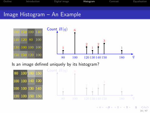
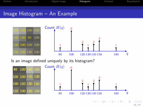
Image Histogram – An Example
180 150 100 140
140 120 80 100
130 100 100 100
150 150 120 100
Count H(q)
q80 100 120 130 140 150 180
1
6
21
23
1
Is an image defined uniquely by its histogram?
Count H(q)
q80 100 120 130 140 150 180
1
6
21
23
1
16 / 47
Outline Introduction Digital image Histogram Contrast Equalisation
Image Histogram – An Example
180 150 100 140
140 120 80 100
130 100 100 100
150 150 120 100
Count H(q)
q80 100 120 130 140 150 180
1
6
21
23
1
Is an image defined uniquely by its histogram?
Count H(q)
q80 100 120 130 140 150 180
1
6
21
23
1
16 / 47

Outline Introduction Digital image Histogram Contrast Equalisation
Histograms of Under- / Over-Exposed Photos
Under-exposure
Over-exposure
17 / 47

Outline Introduction Digital image Histogram Contrast Equalisation
Cumulative Histogram
H = [40, 0, 18, 6, 10, 3, 7, 16] → C = [40, 40, 58, 64, 74, 77, 84, 100]
A cumulative histogram C = [C(q) : q = 0, . . . , 255]
is a mapping that counts the total number of pixel intensities in all
the histogram’s bins up to the current bin q: C(q) =q∑i=0
H(i).
The cumulative histogram is useful for some pixel-wise intensitycorrection, e.g. histogram equalisation.
18 / 47

Outline Introduction Digital image Histogram Contrast Equalisation
Cumulative Histogram – An Example
180 150 100 140
140 120 80 100
130 100 100 100
150 150 120 100
Count H(q)
q80 100 120 130 140 150 180
1
6
21
23
1
Cumulative count C(q)
q80 100 120 130 140 150 18080 100 120 130 140 150 180
1
79 10
1215 16
19 / 47

Outline Introduction Digital image Histogram Contrast Equalisation
Using Histograms
An image histogram is a useful tool for assessing the brightnessand contrast of an image.
Look at the image histograms:
• The majority of intensities forthe accompanying dark imageare distributed to the left.
• The majority of intensities forthe accompanying light imageare distributed to the right.
20 / 47

Outline Introduction Digital image Histogram Contrast Equalisation
Image Negation
The negative of an image with grey levels in the range [0, 255]: bythe negation (negative transformation) g(x, y) = 255− f(x, y)
It reverses the grey values, that is,produces a negative-like image withthe reversed histogram.
21 / 47

Outline Introduction Digital image Histogram Contrast Equalisation
Negation: An Example
155 155 175 55
155 205 75 85
175 75 105 125
55 105 125 125
g(x, y) = 255− f(x, y)
f(x,y) g(x,y)
55 20075 18085 170
105 150125 130155 100175 80205 50
g
f
0 2550
255
100 100 80 200
100 50 180 170
80 180 150 130
200 150 130 130
22 / 47

Outline Introduction Digital image Histogram Contrast Equalisation
Image Contrast
Informally, the contrast of an image g = (g(x, y) : (x, y) ∈ R) isthe difference in visual properties (e.g. brightness or colour) thatmakes a depicted object distinguishable in the image.
• E.g. the object is darker or brighter than other objects at itsbackground.
Some possible ways to formalise and compute contrast:
gmax − gmin
gmax + gminorg(x, y)− gb
gb
• gmax and gmin – the maximum and minimum imagebrightness, respectively.
• gb – a background pixel value.23 / 47

Outline Introduction Digital image Histogram Contrast Equalisation
Image Contrast: An Example
Original image:
Higher contrast:
24 / 47

Outline Introduction Digital image Histogram Contrast Equalisation
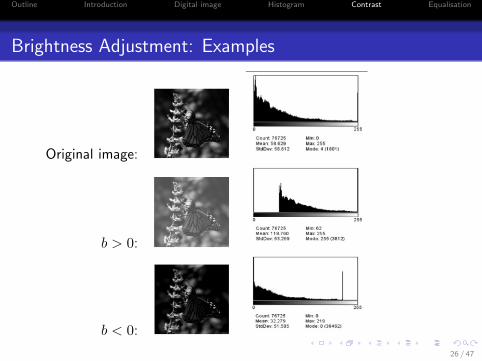
Brightness Adjustment
Adjustment by adding a constant offset, or bias b to pixel values ofan image g to form the new image f :
f(x, y) = g(x, y) + b
b > 0
The brightness increases if b > 0 and decreases if b < 0.
25 / 47
Outline Introduction Digital image Histogram Contrast Equalisation
Brightness Adjustment: Examples
Original image:
b > 0:
b < 0:
26 / 47
Outline Introduction Digital image Histogram Contrast Equalisation
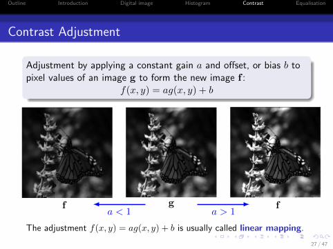
Contrast Adjustment
Adjustment by applying a constant gain a and offset, or bias b topixel values of an image g to form the new image f :
f(x, y) = ag(x, y) + b
f g fa > 1a < 1
The adjustment f(x, y) = ag(x, y) + b is usually called linear mapping.
27 / 47

Outline Introduction Digital image Histogram Contrast Equalisation
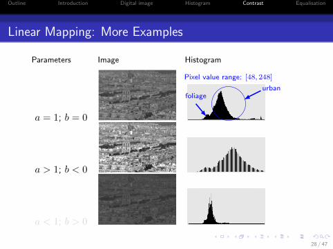
Linear Mapping: More Examples
Parameters Image Histogram
a = 1; b = 0
foliageurban
Pixel value range: [48, 248]
a > 1; b < 0
a < 1; b > 0
28 / 47
Outline Introduction Digital image Histogram Contrast Equalisation
Linear Mapping: More Examples
Parameters Image Histogram
a = 1; b = 0
foliageurban
Pixel value range: [48, 248]
a > 1; b < 0
a < 1; b > 0
28 / 47

Outline Introduction Digital image Histogram Contrast Equalisation
Linear Mapping: More Examples
Parameters Image Histogram
a = 1; b = 0
foliageurban
Pixel value range: [48, 248]
a > 1; b < 0
a < 1; b > 0
28 / 47

Outline Introduction Digital image Histogram Contrast Equalisation
Contrast Adjustment
Contrast adjustment (also called normalisation) increases thedynamic range of intensities in low-contrast images.
Main reasons for acquiring low-contrast images:
• Poor illumination conditions.
• Poor image sensor dynamics.
• Incorrect setting of the lens aperture.
Contrast adjustment:“stretching” pixel-wise grey values(intensities) to span a larger range of values.
• Typically, the full range of grey values, e.g. 0 to 255 in an8-bit greyscale image.
• Improving visual contrast of an image.
29 / 47

Outline Introduction Digital image Histogram Contrast Equalisation
Contrast Adjustment
• An original image f : the lowest, flow, and highest, fhigh, pixelvalues considered for stretching.• flow and fhigh are not necessarily the min and max pixel values.
• The new lower, gmin, and upper, gmax, pixel values.
• Stretching (adjusting, or normalising) f into the image g:
sout = (f(x, y)− flow)(gmax−gminfhigh−flow
)+ gmin
g(x, y) =
gmin if sout < gmin
sout if gmin ≤ sout ≤ gmax
gmax if sout > gmax
• Simply selecting flow and fhigh as the max and min values in theimage f can cause unrepresentative scaling due to outliers.
• More robust: the 5th and 95th percentiles of the histogram for f .
30 / 47
Outline Introduction Digital image Histogram Contrast Equalisation
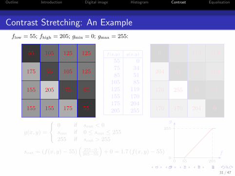
Contrast Stretching: An Example
flow = 55; fhigh = 205; gmin = 0; gmax = 255:
155 155 175 55
155 205 75 85
175 75 105 125
55 105 125 125
g(x, y) =
0 if sout < 0sout if 0 ≤ sout ≤ 255255 if sout > 255
sout = (f(x, y)− 55)(
255−0205−55
)+ 0 = 1.7 (f(x, y)− 55)
f(x,y) g(x,y)
55 075 3485 51
105 85125 119155 170175 204205 255
g
f
0 55 2050
255
170 170 204 0
170 255 34 51
204 34 85 119
0 85 119 119
31 / 47

Outline Introduction Digital image Histogram Contrast Equalisation
Contrast Stretching by Linear Mapping on Slide 31
sout = 1.7f(x, y)− 93.5; g(x, y) = min {255,max {sout, 0}}:
g
f0 25 50 75 100 125 150 175 200 225 250
0
25
50
75
100
125
150
175
200
225
250
205
255
175
204
155
170
125
119
105
85
85
51
75
34
55
32 / 47
Outline Introduction Digital image Histogram Contrast Equalisation
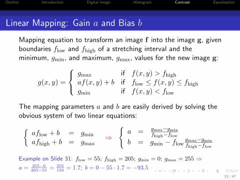
Linear Mapping: Gain a and Bias b
Mapping equation to transform an image f into the image g, givenboundaries flow and fhigh of a stretching interval and theminimum, gmin, and maximum, gmax, values for the new image g:
g(x, y) =
gmax if f(x, y) > fhighaf(x, y) + b if flow ≤ f(x, y) ≤ fhighgmin if f(x, y) < flow
The mapping parameters a and b are easily derived by solving theobvious system of two linear equations:{
aflow + b = gmin
afhigh + b = gmax⇒
{a = gmax−gmin
fhigh−flowb = gmin − flow gmax−gmin
fhigh−flow
Example on Slide 31: flow = 55; fhigh = 205; gmin = 0; gmax = 255 ⇒a = 255−0
205−55= 255
150= 1.7; b = 0− 55 · 1.7 = −93.5
33 / 47

Outline Introduction Digital image Histogram Contrast Equalisation
From the Image Min-Max to the Full [0, 255] Range
flow = fmin = 38; fhigh = fmax = 224; gmin = 0; gmax = 255:
g(x, y) = (f(x, y)− 38) 255−0224−38
= 1.37f(x, y)− 52.1
34 / 47
Outline Introduction Digital image Histogram Contrast Equalisation
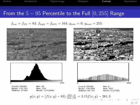
From the 5− 95 Percentile to the Full [0, 255] Range
flow = f5% = 83; fhigh = f95% = 164; gmin = 0; gmax = 255:
g(x, y) = (f(x, y)− 83) 255−0164−83
= 3.15f(x, y)− 261.3
35 / 47
Outline Introduction Digital image Histogram Contrast Equalisation
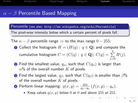
α− β Percentile Based Mapping
Percentile (see also: http://en.wikipedia.org/wiki/Percentile)
The pixel-wise intensity below which a certain percent of pixels fall.
The α− β percentile range ⇒ to the max range 0− 255:
1 Collect the histogram H = (H(q) : q ∈ Q) and compute the
cumulative histogram C = (C(q) : q ∈ Q); C(q) =q∑j=0
H(j).
2 Find the smallest value, qα, such that C(qα) is larger thanα% of the overall number K of pixels.
3 Find the largest value, qβ, such that C(qβ) is smaller than β%of the overall number K of pixels.
4 Perform linear mapping: g(x, y) = 255qβ−qα (f(x, y)− qα).
• Keep values g(x, y) below 0 at 0 and above 255 at 255.
36 / 47
Outline Introduction Digital image Histogram Contrast Equalisation
Histogram Equalisation
A non-linear mapping of pixel-wise intensities aimed at flatteningthe image histogram (distributing evenly the output intensities).
• It increases the dynamic range and, as a result, increases theimage contrast.
• It may be useful in images with both bright or both darkbackgrounds and foregrounds.
• It tends to reveal details that would be otherwise hidden.
• It often produces unrealistic effects in photographs, but is veryuseful in scientific e.g. x-ray, satellite, or thermal) images.
It differs from contrast stretching in the use of non-linear transferfunctions to map between the input and output intensities.
• The mapping function is derived from the image histogram.
37 / 47

Outline Introduction Digital image Histogram Contrast Equalisation
Histogram Equalisation
⇐ An example of an image withpoor contrast.
⇑ The histogram confirms just whatwe can see by visual inspection: thisimage has poor dynamic range.
38 / 47

Outline Introduction Digital image Histogram Contrast Equalisation
Histogram Equalisation
⇐ The same image afterequalisation.
⇑ Now the histogram shows a muchmore even distribution of values.What will the cumulative histogramfor this image look like?
39 / 47

Outline Introduction Digital image Histogram Contrast Equalisation
Histogram Equalisation Algorithm
Given an image f and its histogram H = (H(q) : q = 0, 1, . . . , Q):
1: Compute the cumulative histogram C
C[0] = H[0]
for q = 1,...,Q do C[q] = C[q-1 ]+ H[q]
2: Convert C into the LUT (lookup table) T
for q = 0,...,Q do
T[q] = Q * ( C[q] - C[0] ) / ( C[Q] - C[0] )
3. Using the LUT T , transform f into the equalised image g
for all pixels (x,y) do g[x,y] = T[ f[x,y] ]
40 / 47
Outline Introduction Digital image Histogram Contrast Equalisation
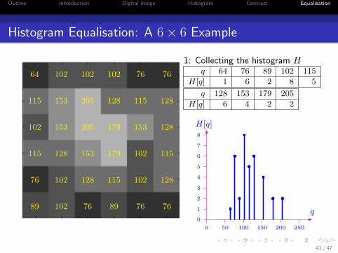
Histogram Equalisation: A 6× 6 Example
64 102 102 102 76 76
115 153 205 128 115 128
102 153 205 179 153 128
115 128 153 179 102 115
76 102 128 115 102 128
89 102 76 89 76 76
1: Collecting the histogram Hq 064 076 089 102 115
H[q] 1 6 2 8 5
q 128 153 179 205
H[q] 6 4 2 2
H[q]
q
0 50 100 150 200 250
0
1
2
3
4
5
6
7
8
41 / 47

Outline Introduction Digital image Histogram Contrast Equalisation
Histogram Equalisation: A 6× 6 Example
2: Computing the cumulative histogram C and the LUT Tq 064 076 089 102 115 128 153 179 205
H[q] 1 6 2 8 5 6 4 2 2
C[q] 1 7 9 17 22 28 32 34 36
T [q] 0 44 58 117 153 197 226 240 255
T [q] C[q]
q
0 50 100 150 200 2500
50
100
150
200
250
5
10
15
20
25
30
35C[q] =
q∑j=0
H[q]
T [q] = round{255 · C[q]−C[64]
C[205]−C[64]
}= round
{255 · C[q]−1
36−1
}= round {7.286 · (C[q]− 1)}
round{z} – the closest to z integer number:e.g. round{3.45} = 3 and round{3.51} = 4.
42 / 47

Outline Introduction Digital image Histogram Contrast Equalisation
Histogram Equalisation: A 6× 6 Example
3: Transforming f in line with the LUT T : g(x, y) = T [f(x, y)].
0 117 117 117 44 44
255117 226 197 153 197
255 240117 226 226 197
240153 197 226 117 153
44 117 197 153 117 197
58 117 44 58 44 44
q 000 044 058 117 153
Hg[q] 1 6 2 8 5
q 197 226 240 255
Hg[q] 6 4 2 2
Hg[q]
q
0 50 100 150 200 250
0
1
2
3
4
5
6
7
8
43 / 47

Outline Introduction Digital image Histogram Contrast Equalisation
Histogram Equalisation: A 6× 6 ExampleImage histograms (H) and cumulative histograms (C)
Before equalisation (image f):
H[q]
q
0 50 100 150 200 250
0
1
2
3
4
5
6
7
8
C[q]
q
0 50 100 150 200 250
0
5
10
15
20
25
30
35
After equalisation (image g):
Hg[q]
q
0 50 100 150 200 250
0
1
2
3
4
5
6
7
8
Cg[q]
q
0 50 100 150 200 250
0
5
10
15
20
25
30
35
44 / 47

Outline Introduction Digital image Histogram Contrast Equalisation
Histogram Equalisation Vs. Contrast Stretching
Initial image Min-max stretching
45 / 47

Outline Introduction Digital image Histogram Contrast Equalisation
Histogram Equalisation Vs. Contrast Stretching
Initial image 5− 95 percentile stretching
46 / 47
Outline Introduction Digital image Histogram Contrast Equalisation
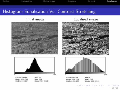
Histogram Equalisation Vs. Contrast Stretching
Initial image Equalised image
47 / 47