Part 2: The Two Approaches to Estimating Confidence · PDF fileApproaches to Estimating ... absence of a sequence of equations leading from some first principles to the procedure described

316 Resampling: The New Statistics

CHAPTER

21

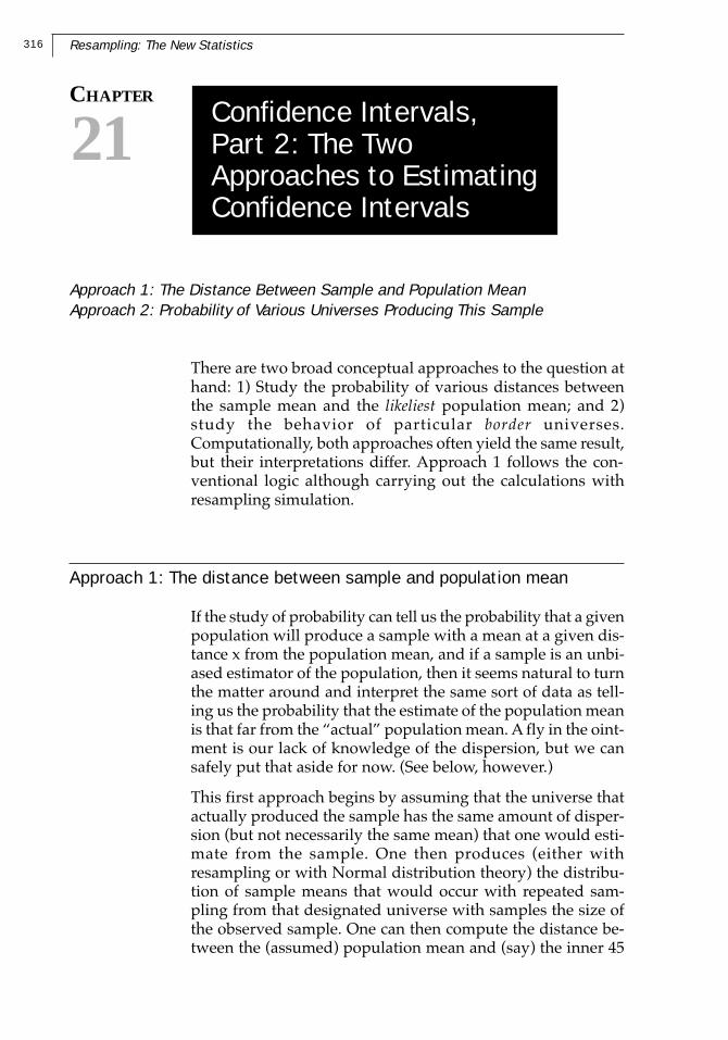
Approach 1: The Distance Between Sample and Population MeanApproach 2: Probability of Various Universes Producing This Sample

Confidence Intervals,Part 2: The TwoApproaches to EstimatingConfidence Intervals

There are two broad conceptual approaches to the question athand: 1) Study the probability of various distances betweenthe sample mean and the likeliest population mean; and 2)study the behavior of particular border universes.Computationally, both approaches often yield the same result,but their interpretations differ. Approach 1 follows the con-ventional logic although carrying out the calculations withresampling simulation.

Approach 1: The distance between sample and population mean

If the study of probability can tell us the probability that a givenpopulation will produce a sample with a mean at a given dis-tance x from the population mean, and if a sample is an unbi-ased estimator of the population, then it seems natural to turnthe matter around and interpret the same sort of data as tell-ing us the probability that the estimate of the population meanis that far from the “actual” population mean. A fly in the oint-ment is our lack of knowledge of the dispersion, but we cansafely put that aside for now. (See below, however.)

This first approach begins by assuming that the universe thatactually produced the sample has the same amount of disper-sion (but not necessarily the same mean) that one would esti-mate from the sample. One then produces (either withresampling or with Normal distribution theory) the distribu-tion of sample means that would occur with repeated sam-pling from that designated universe with samples the size ofthe observed sample. One can then compute the distance be-tween the (assumed) population mean and (say) the inner 45

317Chapter 21—Confidence Intervals, Part 2: Two Approaches to Estimating Confidence Intervals

percent of sample means on each side of the actuallyobservedsample mean.

The crucial step is to shift vantage points. We look from thesample to the universe, instead of from a hypothesized universeto simulated samples (as we have done so far). This same inter-val as computed above must be the relevant distance as whenone looks from the sample to the universe. Putting this alge-braically, we can state (on the basis of either simulation or for-mal calculation) that for any given population S, and for anygiven distance d from its mean mu, that p[(mu xbar) < d] =alpha, where xbar is a randomlygenerated sample mean andalpha is the probability resulting from the simulation or cal-culation.

The above equation focuses on the deviation of various samplemeans (xbar) from a stated population mean (mu). But we arelogically entitled to read the algebra in another fashion, fo-cusing on the deviation of mu from a randomly generatedsample mean. This implies that for any given randomly gen-erated sample mean we observe, the same probability (alpha)describes the probability that mu will be at a distance d or lessfrom the observed xbar. (I believe that this is the logic under-lying the conventional view of confidence intervals, but I haveyet to find a clear-cut statement of it; in any case, it appears tobe logically correct.)

To repeat this difficult idea in slightly different words: If onedraws a sample (large enough to not worry about sample sizeand dispersion), one can say in advance that there is a prob-ability p that the sample mean (xbar) will fall within z stan-dard deviations of the population mean (mu). One estimatesthe population dispersion from the sample. If there is a prob-ability p that xbar is within z standard deviations of mu, thenwith probability p, mu must be within that same z standarddeviations of xbar. To repeat, this is, I believe, the heart of thestandard concept of the confidence interval, to the extent thatthere is thoughtthrough consensus on the matter.

So we can state for such populations the probability that thedistance between the population and sample means will be dor less. Or with respect to a given distance, we can say thatthe probability that the population and sample means will bethat close together is p.

That is, we start by focusing on how much the sample meandiverges from the known population mean. But then—and torepeat once more this key conceptual step—we refocus ourattention to begin with the sample mean and then discuss the


probability that the population mean will be within a givendistance. The resulting distance is what we call the “confidenceinterval.”

Please notice that the distribution (universe) assumed at thebeginning of this approach did not include the assumption thatthe distribution is centered on the sample mean or anywhereelse. It is true that the sample mean is used for purposes of re-porting the location of the estimated universe mean. But despitehow the subject is treated in the conventional approach, theestimated population mean is not part of the work of construct-ing confidence intervals. Rather, the calculations apply in thesame way to all universes in the neighborhood of the sample (whichare assumed, for the purpose of the work, to have the samedispersion). And indeed, it must be so, because the probabil-ity that the universe from which the sample was drawn is cen-tered exactly at the sample mean is very small.

This independence of the confidence-intervals constructionfrom the mean of the sample (and the mean of the estimateduniverse) is surprising at first, but after a bit of thought it makessense.

In this first approach, as noted more generally above, we donot make estimates of the confidence intervals on the basis ofany logical inference from any one particular sample to anyone particular universe, because this cannot be done in principle;it is the futile search for this connection that for decades roiledthe brains of so many statisticians and now continues to troublethe minds of so many students. Instead, we investigate thebehavior of (in this first approach) the universe that has ahigher probability of producing the observed sample than doesany other universe (in the absence of any additional evidenceto the contrary), and whose characteristics are chosen on thebasis of its resemblance to the sample. In this way the estima-tion of confidence intervals is like all other statistical inference:One investigates the probabilistic behavior of one or more hy-pothesized universes, the universe(s) being implicitly sug-gested by the sample evidence but not logically implied bythat evidence. And there are no grounds for dispute about ex-actly what is being done—only about how to interpret the re-sults.

One difficulty with the above approach is that the estimate ofthe population dispersion does not rest on sound foundations;this matter will be discussed later, but it is not likely to lead toa seriously misleading conclusion.

A second difficulty with this approach is in interpreting the


result. What is the justification for focusing our attention on auniverse centered on the sample mean? While this particularuniverse may be more likely than any other, it undoubtedlyhas a low probability. And indeed, the statement of the confi-dence intervals refers to the probabilities that the sample hascome from universes other than the universe centered at thesample mean, and quite a distance from it.

My answer to this question does not rest on a set of meaning-ful mathematical axioms, and I assert that a meaningful axi-omatic answer is impossible in principle. Rather, I reason thatwe should consider the behavior of this universe because otheruniverses near it will produce much the same results, differ-ing only in dispersion from this one, and this difference is notlikely to be crucial; this last assumption is all-important, ofcourse. True, we do not know what the dispersion might befor the “true” universe. But elsewhere (Simon, forthcoming) Iargue that the concept of the “true universe” is not helpful—or maybe even worse than nothing—and should be foresworn.And we can postulate a dispersion for any other universe wechoose to investigate. That is, for this postulation we unabash-edly bring in any other knowledge we may have. The defensefor such an almost-arbitrary move would be that this is a sec-ond-order matter relative to the location of the estimated uni-verse mean, and therefore it is not likely to lead to serious er-ror. (This sort of approximative guessing sticks in the throatsof many trained mathematicians, of course, who want to feelan unbroken logic leading backwards into the mists of axiomformation. But the axioms themselves inevitably are chosenarbitrarily just as there is arbitrariness in the practice at hand,though the choice process for axioms is less obvious and morehallowed by having been done by the masterminds of the past.[See Simon, forthcoming, on the necessity for judgment.] Theabsence of a sequence of equations leading from some firstprinciples to the procedure described in the paragraph aboveis evidence of what is felt to be missing by those who cravelogical justification. The key equation in this approach is for-mally unassailable, but it seems to come from nowhere.)

In the examples in the following chapter may be found com-putations for two population distributions—one binomial andone quantitative—of the histograms of the sample means pro-duced with this procedure.

Operationally, we use the observed sample mean, togetherwith an estimate of the dispersion from the sample, to esti-mate a mean and dispersion for the population. Then with ref-erence to the sample mean we state a combination of a dis-


tance (on each side) and a probability pertaining to the popu-lation mean. The computational examples will illustrate thisprocedure.

Once we have obtained a numerical answer, we must decidehow to interpret it. There is a natural and almost irresistibletendency to talk about the probability that the mean of theuniverse lies within the intervals, but this has proven confus-ing and controversial. Interpretation in terms of a repeatedprocess is not very satisfying intuitively1 . In my view, it is not

1 An example of this sort of interpretation is as follows: specific sample meanXbar that we happen to observe is almost certain to be a bit high or a bitlow. Accordingly, if we want to be reasonably confident that our inferenceis correct, we cannot claim that mu is precisely equal to the observed Xbar.Instead, we must construct an interval estimate or confidence interval ofthe form: mu = Xbar + sampling error

The crucial question is: How wide must this allowance for sampling errorbe? The answer, of course, will depend on how much Xbar fluctuates...

Constructing 95% confidence intervals is like pitching horseshoes. In eachthere is a fixed target, either the population mu or the stake. We are tryingto bracket it with some chancy device, either the random interval or thehorseshoe...

There are two important ways, however, that confidence intervals differfrom pitching horseshoes. First, only one confidence interval is customar-ily constructed. Second, the target mu is not visible like a horseshoe stake.Thus, whereas the horseshoe player always knows the score (and specifi-cally, whether or not the last toss bracketed the stake), the statistician doesnot. He continues to “throw in the dark,” without knowing whether or nota specific interval estimate has bracketed mu. All he has to go on is thestatistical theory that assures him that, in the long run, he will succeed 95%of the time. (Wonnacott and Wonnacott, 1990, p. 258).

Savage refers to this type of interpretation as follows: whenever its advo-cates talk of making assertions that have high probability, whether in con-nection with testing or estimation, they do not actually make such asser-tions themselves, but endlessly pass the buck, saying in effect, “This asser-tion has arisen according to a system that will seldom lead you to makefalse assertions, if you adopt it. As for myself, I assert nothing but the prop-erties of the system.”(1972, pp. 260261)

Lee writes at greater length: “[T]he statement that a 95% confidence inter-val for an unknown parameter ran from 2 to +2 sounded as if the param-eter lay in that interval with 95% probability and yet I was warned that all Icould say was that if I carried out similar procedures time after time thenthe unknown parameters would lie in the confidence intervals I constructed95% of the time.

“Subsequently, I discovered that the whole theory had been worked out invery considerable detail in such books as Lehmann (1959, 1986). But at-tempts such as those that Lehmann describes to put everything on a firmfoundation raised even more questions.” (Lee, 1989, p. vii)


worth arguing about any “true” interpretation of these com-putations. One could sensibly interpret the computations interms of the odds a decisionmaker, given the evidence, wouldreasonably offer about the relative probabilities that the samplecame from one of two specified universes (one of them prob-ably being centered on the sample); this does provide someinformation on reliability, but this procedure departs from theconcept of confidence intervals.

Example 21-1: Counted Data: The Accuracy of PoliticalPolls

Consider the reliability of a randomly selected 1988 presiden-tial election poll, showing 840 intended votes for Bush and 660intended votes for Dukakis out of 1500 (Wonnacott andWonnacott, 1990, p. 5). Let us work through the logic of thisexample.

What is the question? Stated technically, what are the 95% con-fidence limits for the proportion of Bush supporters in thepopulation? (The proportion is the mean of a binomial popu-lation or sample, of course.) More broadly, within whichbounds could one confidently believe that the population pro-portion was likely to lie? At this stage of the work, we mustalready have translated the conceptual question (in this case,a decisionmaking question from the point of view of the can-didates) into a statistical question. (See Chapter 14 on trans-lating questions into statistical form.)

What is the purpose to be served by answering this question?There is no sharp and clear answer in this case. The goal couldbe to satisfy public curiosity, or strategy planning for a candi-date (though a national proportion is not as helpful for plan-ning strategy as state data would be). A secondary goal mightbe to help guide decisions about the sample size of subsequentpolls.

Is this a “probability” or a “probability-statistics” question?The latter; we wish to infer from sample to population ratherthan the converse.

Given that this is a statistics question: What is the form ofthe statistics question—confidence limits or hypothesis test-ing? Confidence limits.

Given that the question is about confidence limits: What isthe description of the sample that has been observed? a) Theraw sample data—the observed numbers of interviewees are


840 for Bush and 660 for Dukakis—constitutes the best descrip-tion of the universe. The statistics of the sample are the givenproportions—56 percent for Bush, 44 percent for Dukakis.

Which universe? (Assuming that the observed sample is rep-resentative of the universe from which it is drawn, what is yourbest guess about the properties of the universe about whose pa-rameter you wish to make statements? The best guess is thatthe population proportion is the sample proportion—that is,the population contains 56 percent Bush votes, 44 percentDukakis votes.

Possibilities for Bayesian analysis? Not in this case, unlessyou believe that the sample was biased somehow.

Which parameter(s) do you wish to make statements about?Mean, median, standard deviation, range, interquartile range,other? We wish to estimate the proportion in favor of Bush (orDukakis).

Which symbols for the observed entities? Perhaps 56 green and44 yellow balls, if an urn is used, or “0” and “1” if the com-puter is used.

Discrete or continuous distribution? In principle, discrete. (Alldistributions must be discrete in practice.)

What values or ranges of values? “0” or “1.”

Finite or infinite? Infinite—the sample is small relative to thepopulation.

If the universe is what you guess it to be, for which samplesdo you wish to estimate the variation? A sample the same sizeas the observed poll.

Here one may continue either with resampling or with the con-ventional method. Everything done up to now would be thesame whether continuing with resampling or with a standardparametric test.


Conventional Calculational Methods

Estimating the Distribution of Differences Between Sample andPopulation Means With the Normal Distribution.

In the conventional approach, one could in principle work fromfirst principles with lists and sample space, but that wouldsurely be too cumbersome. One could work with binomial pro-portions, but this problem has too large a sample for tree-draw-ing and quincunx techniques; even the ordinary textbook tableof binomial coefficients is too small for this job. Calculatingbinomial coefficients also is a big job. So instead one woulduse the Normal approximation to the binomial formula.

(Note to the beginner: The distribution of means that we ma-nipulate has the Normal shape because of the operation of theLaw of Large Numbers (The Central Limit theorem). Sums andaverages, when the sample is reasonably large, take on thisshape even if the underlying distribution is not Normal. Thisis a truly astonishing property of randomlydrawn samples—the distribution of their means quickly comes to resemble a“Normal” distribution, no matter the shape of the underlyingdistribution. We then standardize it with the standard devia-tion or other devices so that we can state the probability dis-tribution of the sampling error of the mean for any sample ofreasonable size.)

The exercise of creating the Normal shape empirically is sim-ply a generalization of particular cases such as we will latercreate here for the poll by resampling simulation. One can alsogo one step further and use the formula of de Moivre-Laplace-Gauss to describe the empirical distributions, and to serve in-stead of the empirical distributions. Looking ahead now, thedifference between resampling and the conventional approachcan be said to be that in the conventional approach we simplyplot the Gaussian distribution very carefully, and use a for-mula instead of the empirical histograms, afterwards puttingthe results in a standardized table so that we can read themquickly without having to recreate the curve each time we useit. More about the nature of the Normal distribution may befound in Simon (forthcoming).

All the work done above uses the information specified pre-viously—the sample size of 1500, the drawing with replace-ment, the observed proportion as the criterion.


Confidence Intervals Empirically—With Resampling

Estimating the Distribution of Differences Between Sample andPopulation Means By Resampling

What procedure to produce entities? Random selection fromurn or computer.

Simple (single step) or complex (multiple “if” drawings)?Simple.

What procedure to produce resamples? That is, with or with-out replacement? With replacement.

Number of drawings observations in actual sample, and hence,number of drawings in resamples? 1500.

What to record as result of each resample drawing? Mean,median, or whatever of resample? The proportion is what weseek.

Stating the distribution of results: The distribution of propor-tions for the trial samples.

Choice of confidence bounds?: 95%, two tails (choice made bythe textbook that posed the problem).

Computation of probabilities within chosen bounds: Read theprobabilistic result from the histogram of results.

Computation of upper and lower confidence bounds: Locatethe values corresponding to the 2.5th and 97.5th percentile ofthe resampled proportions.

Because the theory of confidence intervals is so abstract (evenwith the resampling method of computation), let us now walkthrough this resampling demonstration slowly, using the con-ventional Approach 1 described previously. We first producea sample, and then see how the process works in reverse toestimate the reliability of the sample, using the Bush-Dukakispoll as an example. The computer program follows below.

Step 1: Draw a sample of 1500 voters from a universe that,based on the observed sample, is 56 percent for Bush, 44 per-cent for Dukakis. The first such sample produced by the com-puter happens to be 53 percent for Bush; it might have been58 percent, or 55 percent, or very rarely, 49 percent for Bush.

Step 2: Repeat step 1 perhaps 400 or 1000 times.


Step 3: Estimate the distribution of means (proportions) ofsamples of size 1500 drawn from this 56-44 percent Bush-Dukakis universe; the resampling result is shown below.

Step 4: In a fashion similar to what was done in steps 13, nowcompute the 95 percent confidence intervals for some otherpostulated universe mean—say 53% for Bush, 47% forDukakis. This step produces a confidence interval that is notcentered on the sample mean and the estimated universe mean,and hence it shows the independence of the procedure fromthat magnitude. And we now compare the breadth of the esti-mated confidence interval generated with the 53-47 percentuniverse against the confidence interval derived from the cor-responding distribution of sample means generated by the“true” Bush-Dukakis population of 56 percent—44 percent. Ifthe procedure works well, the results of the two proceduresshould be similar.

Now we interpret the results using this first approach. The his-togram shows the probability that the difference between thesample mean and the population mean—the error in thesample result—will be about 2.5 percentage points too low. Itfollows that about 47.5 percent (half of 95 percent) of the time,a sample like this one will be between the population meanand 2.5 percent too low. We do not know the actual popula-tion mean. But for any observed sample like this one, we cansay that there is a 47.5 percent chance that the distance be-tween it and the mean of the population that generated it isminus 2.5 percent or less.

Now a crucial step: We turn around the statement just above,and say that there is an 47.5 percent chance that the popula-tion mean is less than three percentage points higher than themean of a sample drawn like this one, but at or above thesample mean. (And we do the same for the other side of thesample mean.) So to recapitulate: We observe a sample and itsmean. We estimate the error by experimenting with one ormore universes in that neighborhood, and we then give theprobability that the population mean is within that margin oferror from the sample mean.


Example 21-2: Measured Data Example—the Bootstrap:A Feed Merchant Experiences Varied Pig Weight GainsWith a New Ration and Wants to be Safe in Advertisingan Average Weight Gain

A feed merchant decides to experiment with a new pig ration—ration A—on twelve pigs. To obtain a random sample, he pro-vides twelve customers (selected at random) with sufficientfood for one pig. After 4 weeks, the 12 pigs experience an av-erage gain of 508 ounces. The weight gain of the individualpigs are as follows: 496, 544, 464, 416, 512, 560, 608, 544, 480,466, 512, 496.

The merchant sees that the ration produces results that arequite variable (from a low of 466 ounces to a high of 560 ounces)and is therefore reluctant to advertise an average weight gainof 508 ounces. He speculates that a different sample of pigsmight well produce a different average weight gain.

Unfortunately, it is impractical to sample additional pigs togain additional information about the universe of weight gains.The merchant must rely on the data already gathered. Howcan these data be used to tell us more about the sampling vari-ability of the average weight gain?

Recalling that all we know about the universe of weight gainsis the sample we have observed, we can replicate that samplemillions of times, creating a “pseudo-universe” that embodiesall our knowledge about the real universe. We can then drawadditional samples from this pseudo-universe and see howthey behave.

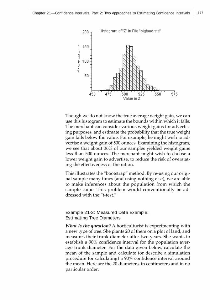
More specifically, we replicate each observed weight gain mil-lions of times—we can imagine writing each result that manytimes on separate pieces of paper—then shuffle those weightgains and pick out a sample of 12. Average the weight gain forthat sample, and record the result. Take repeated samples, andrecord the result for each. We can then make a histogram ofthe results; it might look something like this:


Though we do not know the true average weight gain, we canuse this histogram to estimate the bounds within which it falls.The merchant can consider various weight gains for advertis-ing purposes, and estimate the probability that the true weightgain falls below the value. For example, he might wish to ad-vertise a weight gain of 500 ounces. Examining the histogram,we see that about 36% of our samples yielded weight gainsless than 500 ounces. The merchant might wish to choose alower weight gain to advertise, to reduce the risk of overstat-ing the effectiveness of the ration.

This illustrates the “bootstrap” method. By re-using our origi-nal sample many times (and using nothing else), we are ableto make inferences about the population from which thesample came. This problem would conventionally be ad-dressed with the “t-test.”

Example 21-3: Measured Data Example:Estimating Tree Diameters

What is the question? A horticulturist is experimenting witha new type of tree. She plants 20 of them on a plot of land, andmeasures their trunk diameter after two years. She wants toestablish a 90% confidence interval for the population aver-age trunk diameter. For the data given below, calculate themean of the sample and calculate (or describe a simulationprocedure for calculating) a 90% confidence interval aroundthe mean. Here are the 20 diameters, in centimeters and in noparticular order:


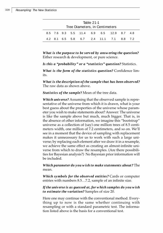
Table 21-1Tree Diameters, in Centimeters

8.5 7.6 9.3 5.5 11.4 6.9 6.5 12.9 8.7 4.8

4.2 8.1 6.5 5.8 6.7 2.4 11.1 7.1 8.8 7.2

What is the purpose to be served by answering the question?Either research & development, or pure science.

Is this a “probability” or a “statistics” question? Statistics.

What is the form of the statistics question? Confidence lim-its.

What is the description of the sample that has been observed?The raw data as shown above.

Statistics of the sample? Mean of the tree data.

Which universe? Assuming that the observed sample is repre-sentative of the universe from which it is drawn, what is yourbest guess about the properties of the universe whose param-eter you wish to make statements about? Answer: The universeis like the sample above but much, much bigger. That is, inthe absence of other information, we imagine this “bootstrap”universe as a collection of (say) one million trees of 8.5 centi-meters width, one million of 7.2 centimeters, and so on. We’llsee in a moment that the device of sampling with replacementmakes it unnecessary for us to work with such a large uni-verse; by replacing each element after we draw it in a resample,we achieve the same effect as creating an almost-infinite uni-verse from which to draw the resamples. (Are there possibili-ties for Bayesian analysis?) No Bayesian prior information willbe included.

Which parameter do you wish to make statements about? Themean.

Which symbols for the observed entities? Cards or computerentries with numbers 8.5…7.2, sample of an infinite size.

If the universe is as guessed at, for which samples do you wishto estimate the variation? Samples of size 20.

Here one may continue with the conventional method. Every-thing up to now is the same whether continuing withresampling or with a standard parametric test. The informa-tion listed above is the basis for a conventional test.


Continuing with resampling:

What procedure will be used to produce the trial entities?Random selection:Simple (single step), not complex (multiple “if”) sample draw-ings).

What procedure to produce resamples? With replacement. Asnoted above, sampling with replacement allows us to foregocreating a very large bootstrap universe; replacing the elementsafter we draw them achieves the same effect as would an infi-nite universe.

Number of drawings? 20 trees

What to record as result of resample drawing? The mean.

How to state the distribution of results? See histogram.

Choice of confidence bounds: 90%, two-tailed.

Computation of values of the resample statistic correspond-ing to chosen confidence bounds: Read from histogram.

As has been discussed in Chapter 13, it often is more appro-priate to work with the median than with the mean. One rea-son is that the median is not so sensitive to the extreme obser-vations as is the mean. Another reason is that one need notassume a Normal distribution for the universe under study:this consideration affects conventional statistics but usuallydoes not affect resampling, but it is worth keeping mind whena statistician is making a choice between a parametric (that is,Normal-based) and a non-parametric procedure.

Example 21-4: Determining a Confidence Interval for theMedian Aluminum Content in Theban Jars

Data for the percentages of aluminum content in a sample of18 ancient Theban jars (Desphpande et. al., 1996, p. 31) are asfollows, arranged in ascending order: 11.4, 13.4, 13.5, 13.8, 13.9,14.4, 14.5, 15.0, 15.1, 15.8, 16.0, 16.3, 16.5, 16.9, 17.0, 17.2, 17.5,19.0. Consider now putting a confidence interval around themedian of 15.45 (halfway between the middle observations15.1 and 15.8).

One may simply estimate a confidence interval around themedian with a bootstrap procedure by substituting the me-dian for the mean in the usual bootstrap procedure for esti-mating a confidence limit around the mean, as follows:


DATA (11.4 13.4 13.5 13.8 13.9 14.4 14.5 15.0 15.1 15.8 16.016.3 16.5 16.9 17.0 17.2 17.5 19.0) c

REPEAT 1000

SAMPLE 18 c c$

MEDIAN c$ d$

SCORE d$ z

END

HISTOGRAM z

PERCENTILE z (2.5 97.5) k

PRINT K

This problem would be approached conventionally with a bi-nomial procedure leading to quite wide confidence intervals(Deshpande, p. 32).

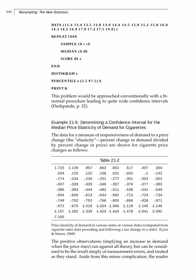
Example 21-5: Determining a Confidence Interval for theMedian Price Elasticity of Demand for Cigarettes

The data for a measure of responsiveness of demand to a pricechange (the “elasticity”—percent change in demand dividedby percent change in price) are shown for cigarette pricechanges as follows:

Table 21-2

1.725 1.139 .957 .863 .802 .517 .407 .304

.204 .125 .122 .106 .031 -.032 -.1 -.142

-.174 -.234 -.240 -.251 -.277 -.301 -.302 -.302

-.307 -.328 -.329 -.346 -.357 -.376 -.377 -.383

-.385 -.393 -.444 -.482 -.511 -.538 -.541 -.549

-.554 -.600 -.613 -.644 -.692 -.713 -.724 -.734

-.749 -.752 -.753 -.766 -.805 -.866 -.926 -.971

-.972 -.975 -1.018 -1.024 -1.066 -1.118 -1.145 -1.146

-1.157 -1.282 -1.339 -1.420 -1.443 -1.478 -2.041 -2.092

-7.100

Price elasticity of demand in various states at various dates (computed fromcigarette sales data preceding and following a tax change in a state) (Lyon& Simon, 1968)

The positive observations (implying an increase in demandwhen the price rises) run against all theory, but can be consid-ered to be the result simply of measurement errors, and treatedas they stand. Aside from this minor complication, the reader


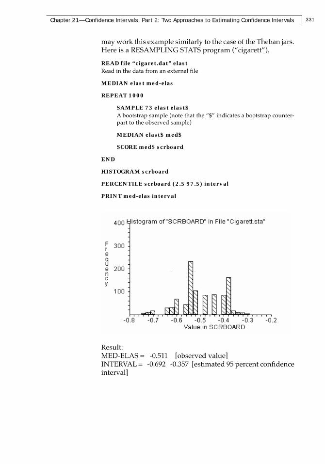
may work this example similarly to the case of the Theban jars.Here is a RESAMPLING STATS program (“cigarett”).

READ file “cigaret.dat” elastRead in the data from an external file

MEDIAN elast med-elas

REPEAT 1000

SAMPLE 73 elast elast$A bootstrap sample (note that the “$” indicates a bootstrap counter-part to the observed sample)

MEDIAN elast$ med$

SCORE med$ scrboard

END

HISTOGRAM scrboard

PERCENTILE scrboard (2.5 97.5) interval

PRINT med-elas interval

Result:MED-ELAS = -0.511 [observed value]INTERVAL = -0.692 -0.357 [estimated 95 percent confidenceinterval]


Example 21-6: Measured Data Example: Confidence Inter-vals For a Difference Between Two Means, the Mice DataAgain

Returning to the data on the survival times of the two groupsof mice in Example 18-4: It is the view of this book that confi-dence intervals should be calculated for a difference betweentwo groups only if one is reasonably satisfied that the differ-ence is not due to chance. Some statisticians might choose tocompute a confidence interval in this case nevertheless, somebecause they believe that the confidence-interval machineryis more appropriate to deciding whether the difference is thelikely outcome of chance than is the machinery of a hypoth-esis test in which you are concerned with the behavior of abenchmark or null universe. So let us calculate a confidenceinterval for these data, which will in any case demonstrate thetechnique for determining a confidence interval for a differ-ence between two samples.

Our starting point is our estimate for the difference in meansurvival times between the two samples—30.63 days. We ask“How much might this estimate be in error? If we drew addi-tional samples from the control universe and additionalsamples from the treatment universe, how much might theydiffer from this result?”

We do not have the ability to go back to these universes anddraw more samples, but from the samples themselves we cancreate hypothetical universes that embody all that we knowabout the treatment and control universes. We imagine repli-cating each element in each sample millions of times to createa hypothetical control universe and (separately) a hypotheti-cal treatment universe. Then we can draw samples (separately)from these hypothetical universes to see how reliable is ouroriginal estimate of the difference in means (30.63 days).

Actually, we use a shortcut —instead of copying each sampleelement a million times, we simply replace it after drawing itfor our resample, thus creating a universe that is effectivelyinfinite.

Here are the steps:

Step 1: Consider the two samples separately as the relevantuniverses.

Step 2: Draw a sample of 7 with replacement from the treat-ment group and calculate the mean.


Step 3: Draw a sample of 9 with replacement from the con-trol group and calculate the mean.

Step 4: Calculate the difference in means (treatment minuscontrol) & record.

Step 5: Repeat steps 2-4 many times.

Step 6: Review the distribution of resample means; the 5thand 95th percentiles are estimates of the endpoints of a 90 per-cent confidence interval.

Here is a RESAMPLING STATS program (“mice-ci”):

NUMBERS (94 38 23 197 99 16 141) treatmttreatment group

NUMBERS (52 10 40 104 51 27 146 30 46) controlcontrol group

REPEAT 1000step 5 above

SAMPLE 7 treatmt treatmt$step 2 above

SAMPLE 9 control control$step 3

MEAN treatmt$ tmeanstep 4

MEAN control$ cmeanstep 4

SUBTRACT tmean cmean diffstep 4

SCORE diff scrboardstep 4

ENDstep 5

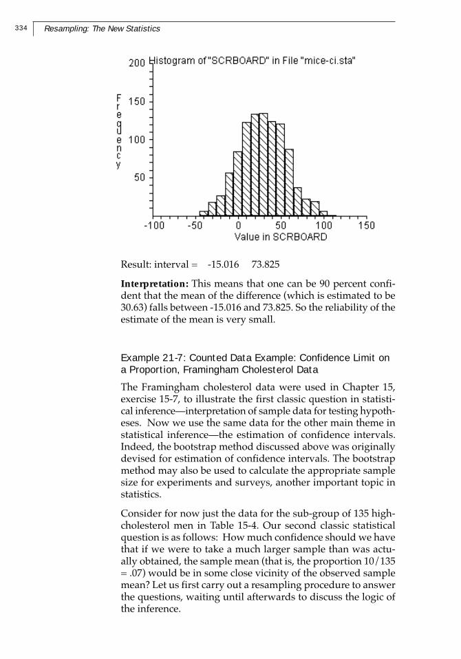
HISTOGRAM scrboard

PERCENTILE scrboard (5 95) intervalstep 6

PRINT interval


Result: interval = -15.016 73.825

Interpretation: This means that one can be 90 percent confi-dent that the mean of the difference (which is estimated to be30.63) falls between -15.016 and 73.825. So the reliability of theestimate of the mean is very small.

Example 21-7: Counted Data Example: Confidence Limit ona Proportion, Framingham Cholesterol Data

The Framingham cholesterol data were used in Chapter 15,exercise 15-7, to illustrate the first classic question in statisti-cal inference—interpretation of sample data for testing hypoth-eses. Now we use the same data for the other main theme instatistical inference—the estimation of confidence intervals.Indeed, the bootstrap method discussed above was originallydevised for estimation of confidence intervals. The bootstrapmethod may also be used to calculate the appropriate samplesize for experiments and surveys, another important topic instatistics.

Consider for now just the data for the sub-group of 135 high-cholesterol men in Table 15-4. Our second classic statisticalquestion is as follows: How much confidence should we havethat if we were to take a much larger sample than was actu-ally obtained, the sample mean (that is, the proportion 10/135= .07) would be in some close vicinity of the observed samplemean? Let us first carry out a resampling procedure to answerthe questions, waiting until afterwards to discuss the logic ofthe inference.


1. Construct an urn containing 135 balls—10 red (infarction)and 125 green (no infarction) to simulate the universe as weguess it to be.

2. Mix, choose a ball, record its color, replace it, and repeat135 times (to simulate a sample of 135 men).

3. Record the number of red balls among the 135 balls drawn.

4. Repeat steps 2-4 perhaps 1000 times, and observe how muchthe total number of reds varies from sample to sample. Wearbitrarily denote the boundary lines that include 47.5 percentof the hypothetical samples on each side of the sample meanas the 95 percent “confidence limits” around the mean of theactual population.

Here is a RESAMPLING STATS program (“myocar3”):

URN 10#1 125#0 menAn urn (called “men”) with ten “1s” (infarctions) and 125 “0s” (no infarc-tion)

REPEAT 1000Do 1000 trials

SAMPLE 135 men aSample (with replacement) 135 numbers from the urn, put them in a

COUNT a =1 bCount the infarctions

DIVIDE b 135 cExpress as a proportion

SCORE c zKeep score of the result

ENDEnd the trial, go back and repeat

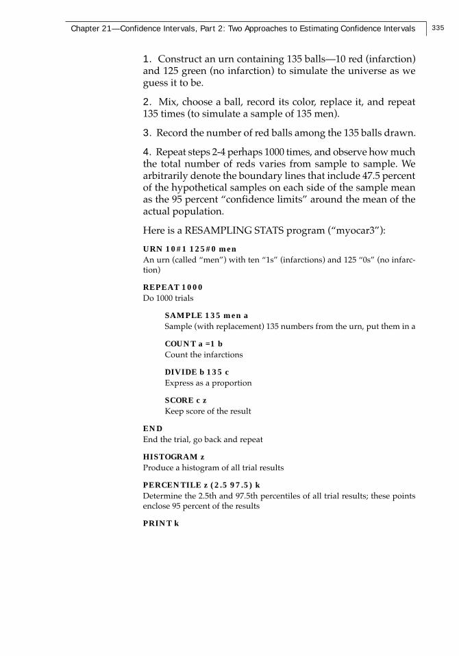
HISTOGRAM zProduce a histogram of all trial results

PERCENTILE z (2.5 97.5) kDetermine the 2.5th and 97.5th percentiles of all trial results; these pointsenclose 95 percent of the results

PRINT k


Proportion with infarction

Result: k = 0.037037 0.11852

(This is the 95 percent confidence interval, enclosing 95 per-cent of the resample results)

The variation in the histogram above highlights the fact that asample containing only 10 cases of infarction is very small, andthe number of observed cases—or the proportion of cases—necessarily varies greatly from sample to sample. Perhaps themost important implication of this statistical analysis, then, isthat we badly need to collect additional data.

Again, this is a classic problem in confidence intervals, foundin all subject fields. The language used in the cholesterol-inf-arction example is exactly the same as the language used forthe Bush-Dukakis poll above except for labels and numbers.

As noted above, the philosophic logic of confidence intervalsis quite deep and controversial, less obvious than for the hy-pothesis test. The key idea is that we can estimate for any givenuniverse the probability P that a sample’s mean will fall withinany given distance D of the universe’s mean; we then turn thisaround and assume that if we know the sample mean, the prob-ability is P that the universe mean is within distance D of it.This inversion is more slippery than it may seem. But the logicis exactly the same for the formulaic method and forresampling. The only difference is how one estimates the prob-abilities—either with a numerical resampling simulation (ashere), or with a formula or other deductive mathematical de-vice (such as counting and partitioning all the possibilities, asGalileo did when he answered a gambler’s question about


three dice). And when one uses the resampling method, theprobabilistic calculations are the least demanding part of thework. One then has mental capacity available to focus on thecrucial part of the job—framing the original question soundly,choosing a model for the facts so as to properly resemble theactual situation, and drawing appropriate inferences from thesimulation.

Approach 2: Probability of various universes producing this sample

A second approach to the general question of estimate accu-racy is to analyze the behavior of a variety of universes cen-tered at other points on the line, rather than the universe cen-tered on the sample mean. One can ask the probability that adistribution centered away from the sample mean, with a givendispersion, would produce (say) a 10-apple scatter having amean as far away from the given point as the observed samplemean. If we assume the situation to be symmetric, we can finda point at which we can say that a distribution centered therewould have only a (say) 5 percent chance of producing theobserved sample. And we can also say that a distribution evenfurther away from the sample mean would have an even lowerprobability of producing the given sample. But we cannot turnthe matter around and say that there is any particular chancethat the distribution that actually produced the observed sampleis between that point and the center of the sample.

Imagine a situation where you are standing on one side of acanyon, and you are hit by a baseball, the only ball in the vi-cinity that day. Based on experiments, you can estimate that abaseball thrower who you see standing on the other side ofthe canyon has only a 5 percent chance of hitting you with asingle throw. But this does not imply that the source of theball that hit you was someone else standing in the middle ofthe canyon, because that is patently impossible. That is, yourknowledge about the behavior of the “boundary” universedoes not logically imply anything about the existence and be-havior of any other universes. But just as in the discussion oftesting hypotheses, if you know that one possibility is unlikely,it is reasonable that as a result you will draw conclusions aboutother possibilities in the context of your general knowledgeand judgment.

We can find the “boundary” distribution(s) we seek if we a)specify a measure of dispersion, and b) try every point along


the line leading away from the sample mean, until we find thatdistribution that produces samples such as that observed witha (say) 5 percent probability or less.

To estimate the dispersion, in many cases we can safely use anestimate based on the sample dispersion, using eitherresampling or Normal distribution theory. The hardest casesfor resampling are a) a very small sample of data, and b) aproportion near 0 or near 1.0 (because the presence or absencein the sample of a small number of observations can changethe estimate radically, and therefore a large sample is neededfor reliability). In such situations one should use additionaloutside information, or Normal distribution theory, or both.

We can also create a confidence interval in the following fash-ion: We can first estimate the dispersion for a universe in thegeneral neighborhood of the sample mean, using various de-vices to be “conservative,” if we like1. Given the estimated dis-persion, we then estimate the probability distribution of vari-ous amounts of error between observed sample means and thepopulation mean. We can do this with resampling simulationas follows: a) Create other universes at various distances fromthe sample mean, but with other characteristics similar to theuniverse that we postulate for the immediate neighborhoodof the sample, and b) experiment with those universes. Onecan also apply the same logic with a more conventional para-metric approach, using general knowledge of the samplingdistribution of the mean, based on Normal distribution theoryor previous experience with resampling. We shall not discussthe latter method here.

As with approach 1, we do not make any probability state-ments about where the population mean may be found. Rather,we discuss only what various hypothetical universes mightproduce, and make inferences about the “actual” population’scharacteristics by comparison with those hypothesized uni-verses.

If we are interested in (say) a 95 percent confidence interval,we want to find the distribution on each side of the samplemean that would produce a sample with a mean that far awayonly 2.5 percent of the time (2 * .025 = 1-.95). A shortcut to findthese “border distributions” is to plot the sampling distribu-

2 More about this later; it is, as I said earlier, not of primary importance inestimating the accuracy of the confidence intervals; note, please, that as wetalk about the accuracy of statements about accuracy, we are moving downthe ladder of sizes of causes of error.


tion of the mean at the center of the sample, as in Approach 1.Then find the (say) 2.5 percent cutoffs at each end of that dis-tribution. On the assumption of equal dispersion at the twopoints along the line, we now reproduce the previously-plot-ted distribution with its centroid (mean) at those 2.5 percentpoints on the line. The new distributions will have 2.5 percentof their areas on the other side of the mean of the sample.

Example 21-8: Approach 2 for Counted Data: the Bush-Dukakis Poll

Let’s implement Approach 2 for counted data, using for com-parison the Bush-Dukakis poll data discussed earlier in thecontext of Approach 1.

We seek to state, for universes that we select on the basis thattheir results will interest us, the probability that they (or it, fora particular universe) would produce a sample as far or far-ther away from the mean of the universe in question as themean of the observed sample—56 percent for Bush. The mostinteresting universe is that which produces such a sample onlyabout 5 percent of the time, simply because of the correspon-dence of this value to a conventional breakpoint in statisticalinference. So we could experiment with various universes bytrial and error to find this universe.

We can learn from our previous simulations of the Bush–Dukakis poll in Approach 1 that about 95 percent of thesamples fall within .025 on either side of the sample mean(which we had been implicitly assuming is the location of thepopulation mean). If we assume (and there seems no reasonnot to) that the dispersions of the universes we experimentwith are the same, we will find (by symmetry) that the uni-verse we seek is centered on those points .025 away from .56,or .535 and .585.

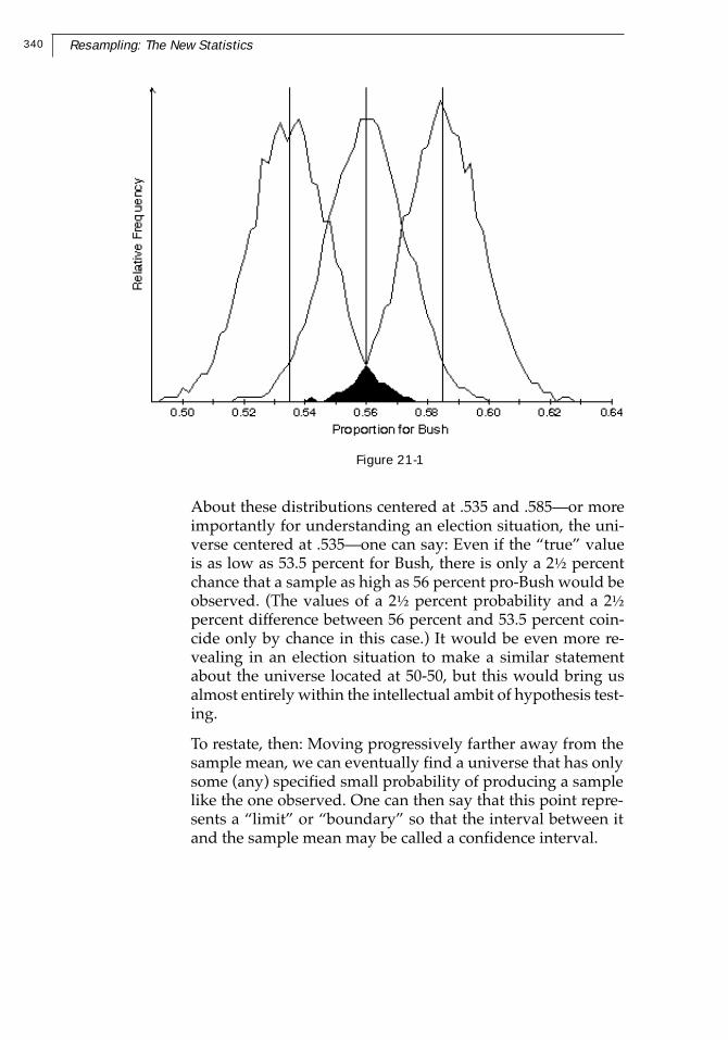
From the standpoint of Approach 2, then, the conventionalsample formula that is centered at the mean can be consid-ered a shortcut to estimating the boundary distributions. Wesay that the boundary is at the point that centers a distribu-tion which has only a (say) 2.5 percent chance of producingthe observed sample; it is that distribution which is the sub-ject of the discussion, and not the distribution which is cen-tered at mu = xbar. Results of these simulations are shown inFigure 21-1.


Figure 21-1

About these distributions centered at .535 and .585—or moreimportantly for understanding an election situation, the uni-verse centered at .535—one can say: Even if the “true” valueis as low as 53.5 percent for Bush, there is only a 2½ percentchance that a sample as high as 56 percent pro-Bush would beobserved. (The values of a 2½ percent probability and a 2½

percent difference between 56 percent and 53.5 percent coin-cide only by chance in this case.) It would be even more re-vealing in an election situation to make a similar statementabout the universe located at 50-50, but this would bring usalmost entirely within the intellectual ambit of hypothesis test-ing.

To restate, then: Moving progressively farther away from thesample mean, we can eventually find a universe that has onlysome (any) specified small probability of producing a samplelike the one observed. One can then say that this point repre-sents a “limit” or “boundary” so that the interval between itand the sample mean may be called a confidence interval.


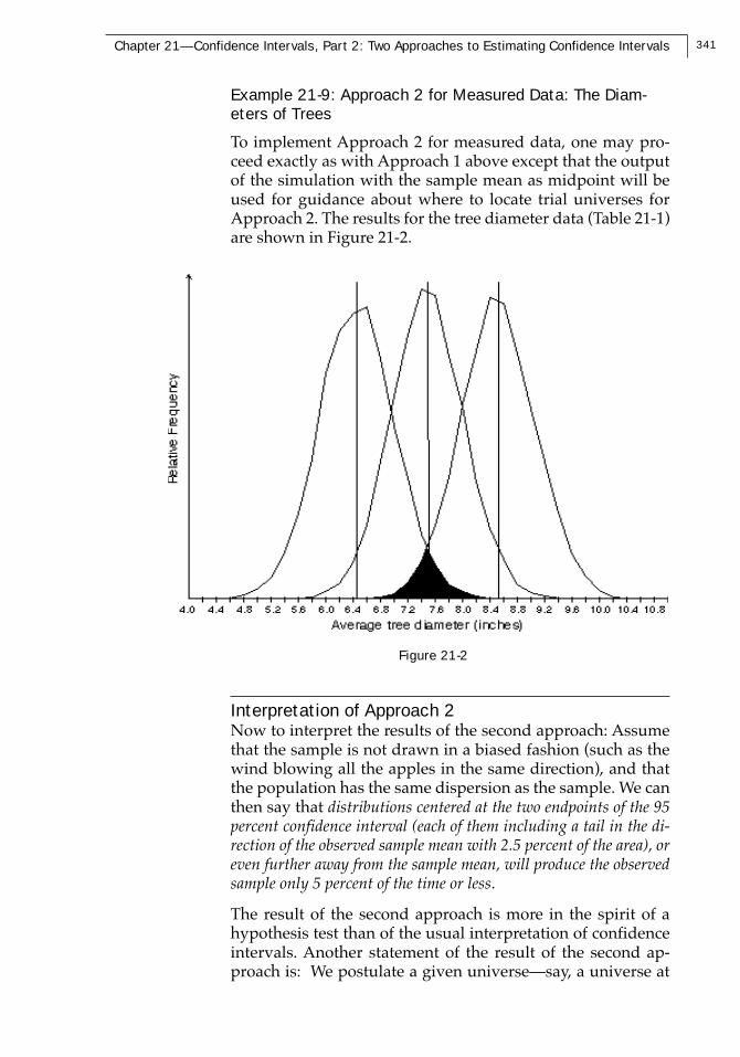
Example 21-9: Approach 2 for Measured Data: The Diam-eters of Trees

To implement Approach 2 for measured data, one may pro-ceed exactly as with Approach 1 above except that the outputof the simulation with the sample mean as midpoint will beused for guidance about where to locate trial universes forApproach 2. The results for the tree diameter data (Table 21-1)are shown in Figure 21-2.

Figure 21-2

Interpretation of Approach 2Now to interpret the results of the second approach: Assumethat the sample is not drawn in a biased fashion (such as thewind blowing all the apples in the same direction), and thatthe population has the same dispersion as the sample. We canthen say that distributions centered at the two endpoints of the 95percent confidence interval (each of them including a tail in the di-rection of the observed sample mean with 2.5 percent of the area), oreven further away from the sample mean, will produce the observedsample only 5 percent of the time or less.

The result of the second approach is more in the spirit of ahypothesis test than of the usual interpretation of confidenceintervals. Another statement of the result of the second ap-proach is: We postulate a given universe—say, a universe at


(say) the two-tailed 95 percent boundary line. We then say: Theprobability that the observed sample would be produced by auniverse with a mean as far (or further) from the observedsample’s mean as the universe under investigation is only 2.5percent. This is similar to the probvalue interpretation of ahypothesis-test framework. It is not a direct statement aboutthe location of the mean of the universe from which the samplehas been drawn. But it is certainly reasonable to derive a bet-ting-odds interpretation of the statement just above, to wit: Thechances are 2½ in 100 (or, the odds are 2½ to 97½) that a popu-lation located here would generate a sample with a mean asfar away as the observed sample. And it would seem legiti-mate to proceed to the further betting-odds statement that (as-suming we have no additional information) the odds are 97 ½to 2½ that the mean of the universe that generated this sampleis no farther away from the sample mean than the mean of theboundary universe under discussion. About this statementthere is nothing slippery, and its meaning should not be con-troversial.

Here again the tactic for interpreting the statistical procedureis to restate the facts of the behavior of the universe that weare manipulating and examining at that moment. We use aheuristic device to find a particular distribution—the one thatis at (say) the 97½–2½ percent boundary—and simply stateexplicitly what the distribution tells us implicitly: The prob-ability of this distribution generating the observed sample (ora sample even further removed) is 2½ percent. We could goon to say (if it were of interest to us at the moment) that be-cause the probability of this universe generating the observedsample is as low as it is, we “reject” the “hypothesis” that thesample came from a universe this far away or further. Or inother words, we could say that because we would be very sur-prised if the sample were to have come from this universe, weinstead believe that another hypothesis is true. The “other”hypothesis often is that the universe that generated the samplehas a mean located at the sample mean or closer to it than theboundary universe.

The behavior of the universe at the 97½–2½ percent boundaryline can also be interpreted in terms of our “confidence” aboutthe location of the mean of the universe that generated the ob-served sample. We can say: At this boundary point lies the endof the region within which we would bet 97½ to 2½ that themean of the universe that generated this sample lies to the (say)right of it.


As noted in the preview to this chapter, we do not learn aboutthe reliability of sample estimates of the population mean (andother parameters) by logical inference from any one particu-lar sample to any one particular universe, because in principlethis cannot be done. Instead, in this second approach we inves-tigate the behavior of various universes at the borderline ofthe neighborhood of the sample, those universes being cho-sen on the basis of their resemblances to the sample. We seek,for example, to find the universes that would produce sampleswith the mean of the observed sample less than (say) 5 per-cent of the time. In this way the estimation of confidence in-tervals is like all other statistical inference: One investigatesthe probabilistic behavior of hypothesized universes, the hy-potheses being implicitly suggested by the sample evidencebut not logically implied by that evidence.

Approaches 1 and 2 may (if one chooses) be seen as identicalconceptually as well as (in many cases) computationally (ex-cept for the asymmetric distributions mentioned earlier). Butas I see it, the interpretation of them is rather different, anddistinguishing them helps one’s intuitive understanding.

Exercises

Solutions for problems may be found in the section titled, “Ex-ercise Solutions” at the back of this book.

Exercise 21-1

In a sample of 200 people, 7 percent are found to be unem-ployed. Determine a 95 percent confidence interval for the truepopulation proportion.

Exercise 21-2

A sample of 20 batteries is tested, and the average lifetime is28.85 months. Establish a 95 percent confidence interval forthe true average value. The sample values (lifetimes in months)are listed below.

30 32 31 28 31 29 29 24 30 31 28 28 32 31 24 23 31 27 2731


Exercise 21-3

Suppose we have 10 measurements of Optical Density on abatch of HIV negative control:

.02 .026 .023 .017 .022 .019 .018 .018 .017 .022

Derive a 95 percent confidence interval for the sample mean.Are there enough measurements to produce a satisfactory an-swer?

Documents

Part 2: The Two Approaches to Estimating Confidence · PDF fileApproaches to Estimating ... absence of a sequence of equations leading from some first principles to the procedure described