Embed Size (px)
Citation preview
Hoare Logic
Hoare Logic is used to reason about the correctness of programs. In the end, it reduces a program and its specification to a set of verifications
conditions.
Slides by Wishnu PrasetyaURL : www.cs.uu.nl/~wishnuCourse URL : www.cs.uu.nl/docs/vakken/pc
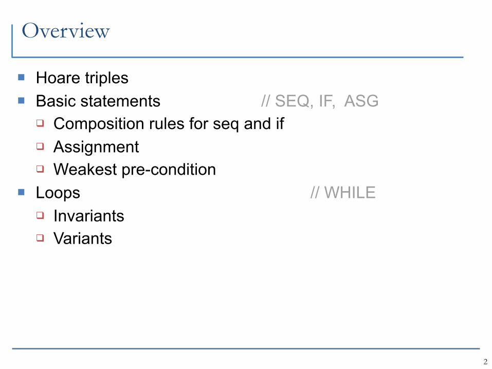
Overview
Hoare triples Basic statements // SEQ, IF, ASG
Composition rules for seq and if Assignment Weakest pre-condition
Loops // WHILE Invariants Variants
2
Hoare triples
3
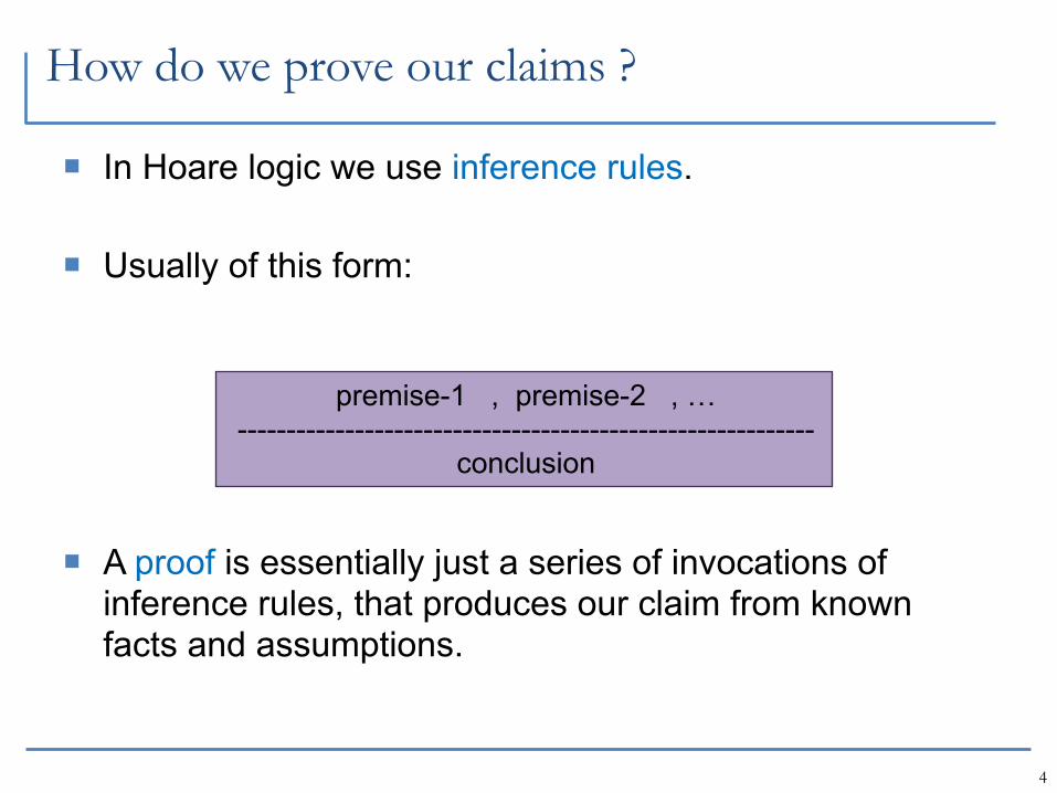
How do we prove our claims ?
In Hoare logic we use inference rules.
Usually of this form:
A proof is essentially just a series of invocations of inference rules, that produces our claim from known facts and assumptions.
4
premise-1 , premise-2 , …-----------------------------------------------------------
conclusion
5
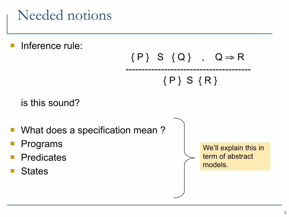
Needed notions
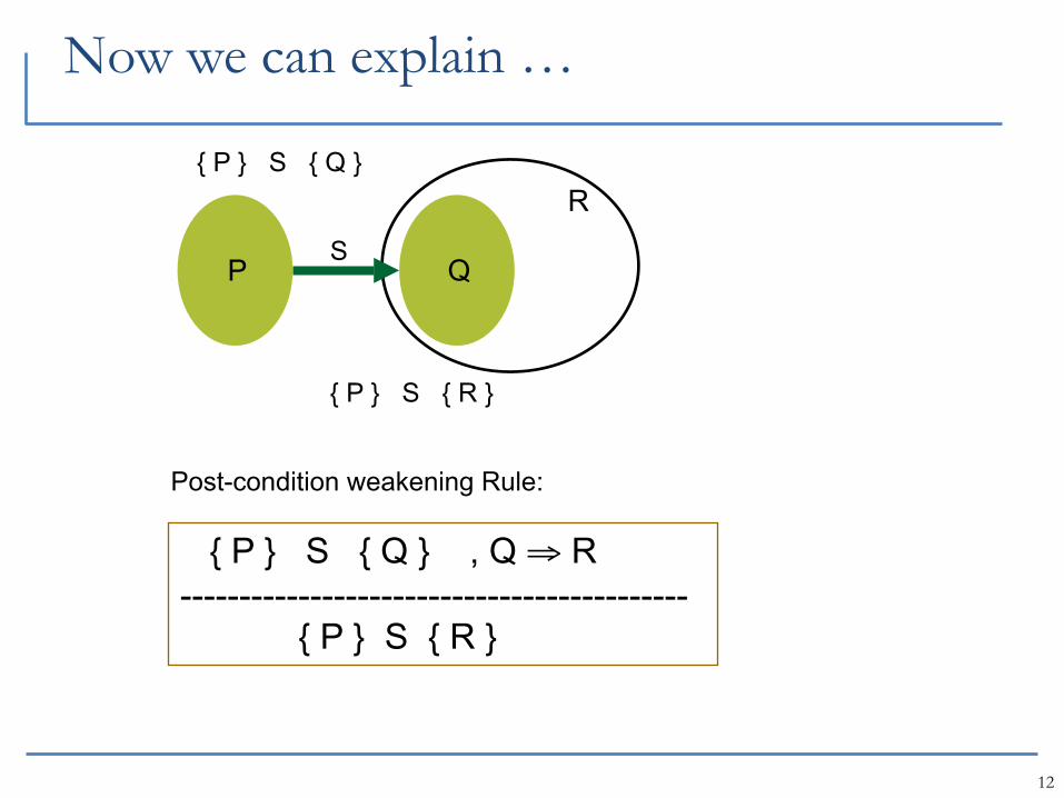
Inference rule: { P } S { Q } , Q ⇒ R --------------------------------------- { P } S { R }
is this sound?
What does a specification mean ? Programs Predicates States
We’ll explain this in term of abstract models.
6
State
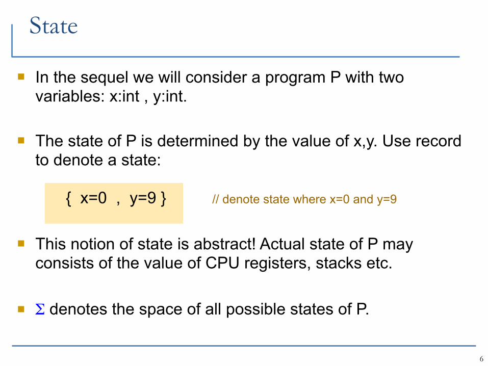
In the sequel we will consider a program P with two variables: x:int , y:int.
The state of P is determined by the value of x,y. Use record to denote a state:
{ x=0 , y=9 } // denote state where x=0 and y=9
This notion of state is abstract! Actual state of P may consists of the value of CPU registers, stacks etc.
Σ denotes the space of all possible states of P.
7
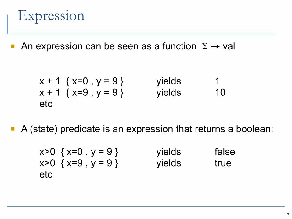
Expression
An expression can be seen as a function Σ → val
x + 1 { x=0 , y = 9 } yields 1 x + 1 { x=9 , y = 9 } yields 10 etc
A (state) predicate is an expression that returns a boolean:
x>0 { x=0 , y = 9 } yields false x>0 { x=9 , y = 9 } yields true etc
8
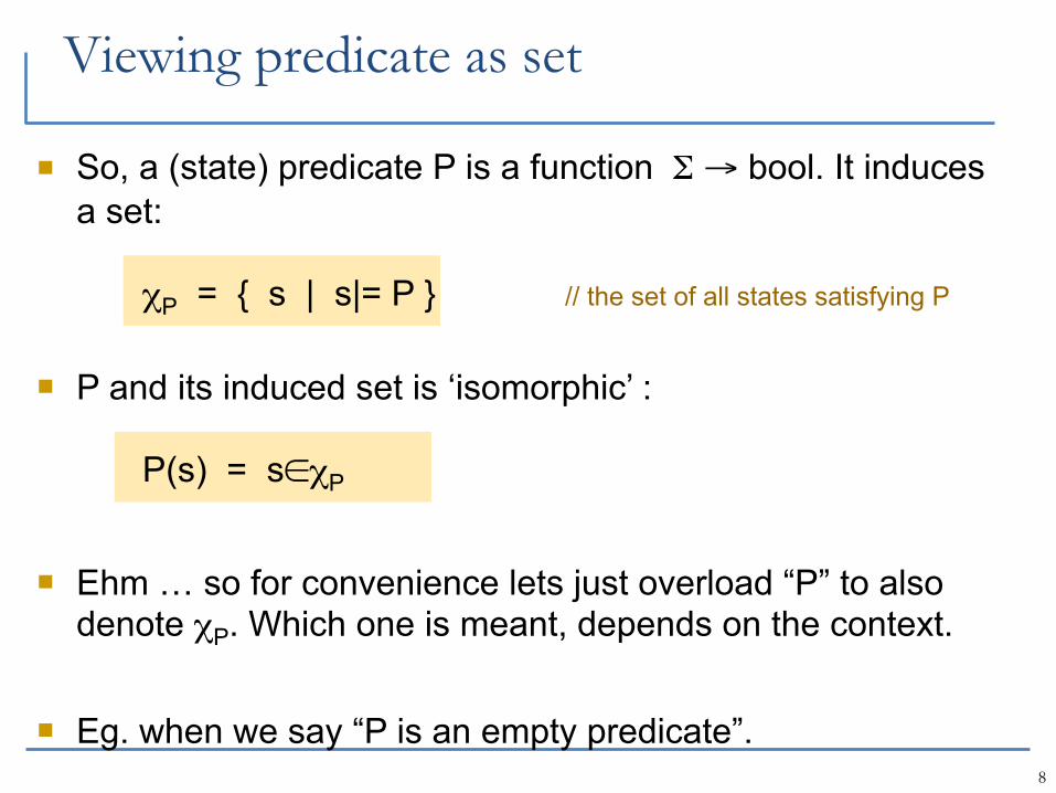
Viewing predicate as set
So, a (state) predicate P is a function Σ → bool. It induces a set:
χP = { s | s|= P } // the set of all states satisfying P
P and its induced set is ‘isomorphic’ :
P(s) = s∈χP
Ehm … so for convenience lets just overload “P” to also denote χP. Which one is meant, depends on the context.
Eg. when we say “P is an empty predicate”.
9
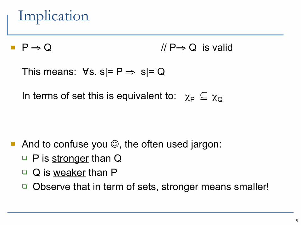
Implication
P ⇒ Q // P⇒ Q is valid
This means: ∀s. s|= P ⇒ s|= Q
In terms of set this is equivalent to: χP ⊆ χQ
And to confuse you , the often used jargon: P is stronger than Q Q is weaker than P Observe that in term of sets, stronger means smaller!
10
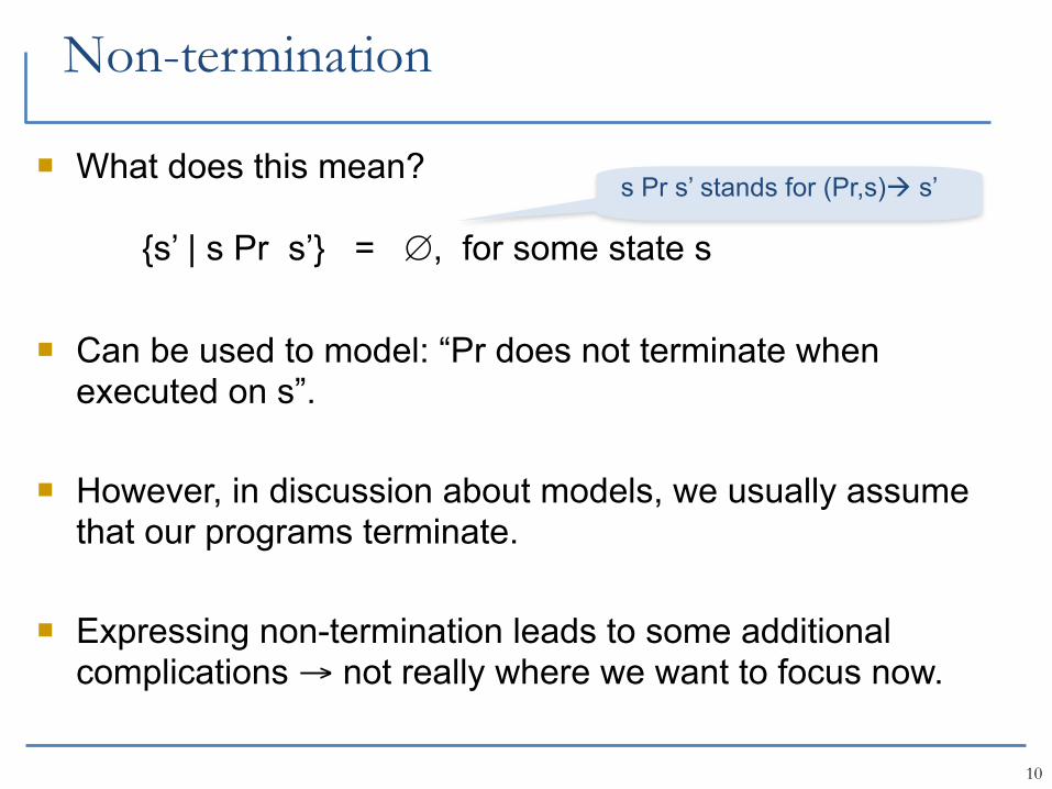
Non-termination
What does this mean?
{s’ | s Pr s’} = ∅, for some state s
Can be used to model: “Pr does not terminate when executed on s”.
However, in discussion about models, we usually assume that our programs terminate.
Expressing non-termination leads to some additional complications → not really where we want to focus now.
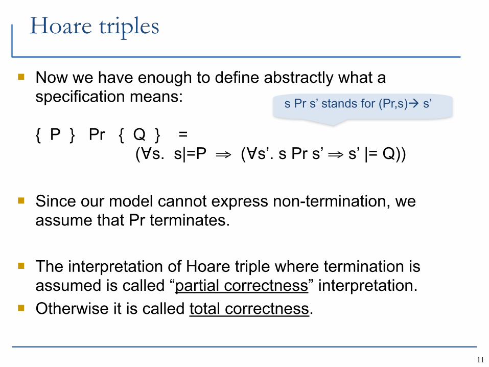
s Pr s’ stands for (Pr,s) s’
11
Hoare triples
Now we have enough to define abstractly what a specification means:
{ P } Pr { Q } = (∀s. s|=P ⇒ (∀s’. s Pr s’ ⇒ s’ |= Q))
Since our model cannot express non-termination, we assume that Pr terminates.
The interpretation of Hoare triple where termination is assumed is called “partial correctness” interpretation.
Otherwise it is called total correctness.
s Pr s’ stands for (Pr,s) s’
12
Now we can explain …
P Q
RS
{ P } S { Q } , Q ⇒ R------------------------------------------- { P } S { R }
Post-condition weakening Rule:
{ P } S { Q }
{ P } S { R }
13
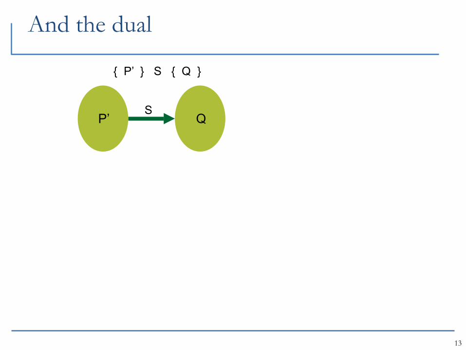
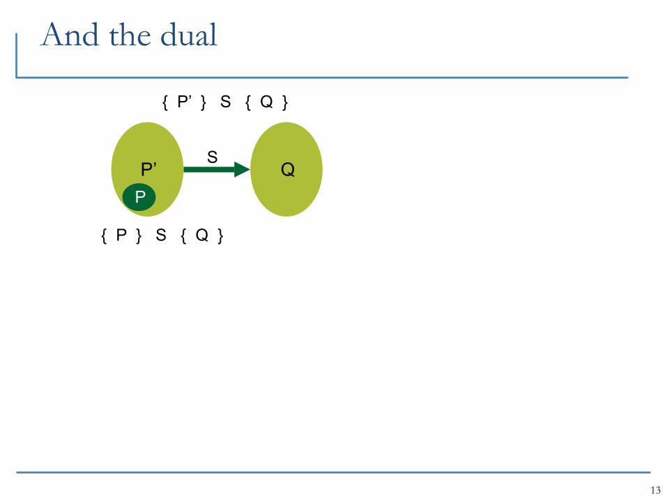
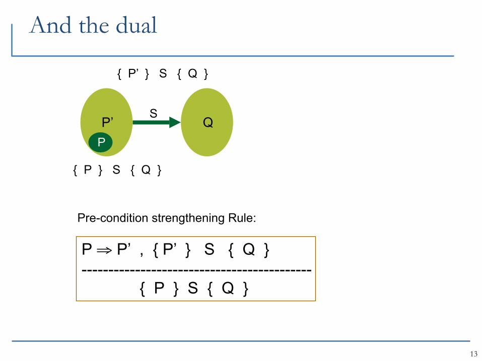
And the dual
P’ QS
{ P’ } S { Q }
13
And the dual
P’ QS
{ P’ } S { Q }
P
{ P } S { Q }
13
And the dual
P’ QS
P ⇒ P’ , { P’ } S { Q } ------------------------------------------- { P } S { Q }
Pre-condition strengthening Rule:
{ P’ } S { Q }
P
{ P } S { Q }
14
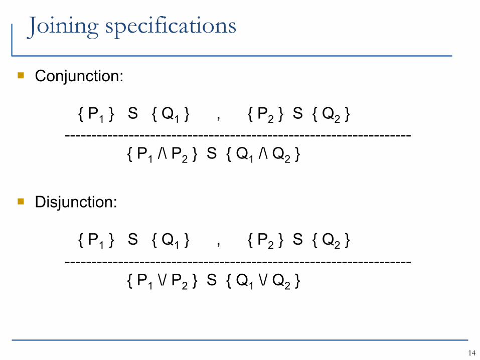
Joining specifications
Conjunction:
{ P1 } S { Q1 } , { P2 } S { Q2 } ----------------------------------------------------------------- { P1 /\ P2 } S { Q1 /\ Q2 }
Disjunction:
{ P1 } S { Q1 } , { P2 } S { Q2 } ----------------------------------------------------------------- { P1 \/ P2 } S { Q1 \/ Q2 }
Reasoning about basic statements
15

1616
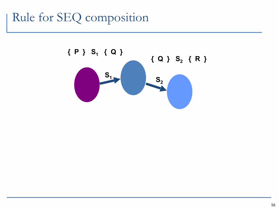
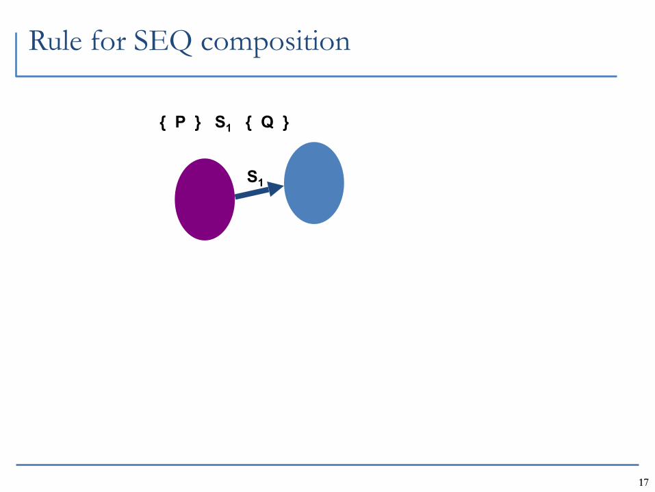
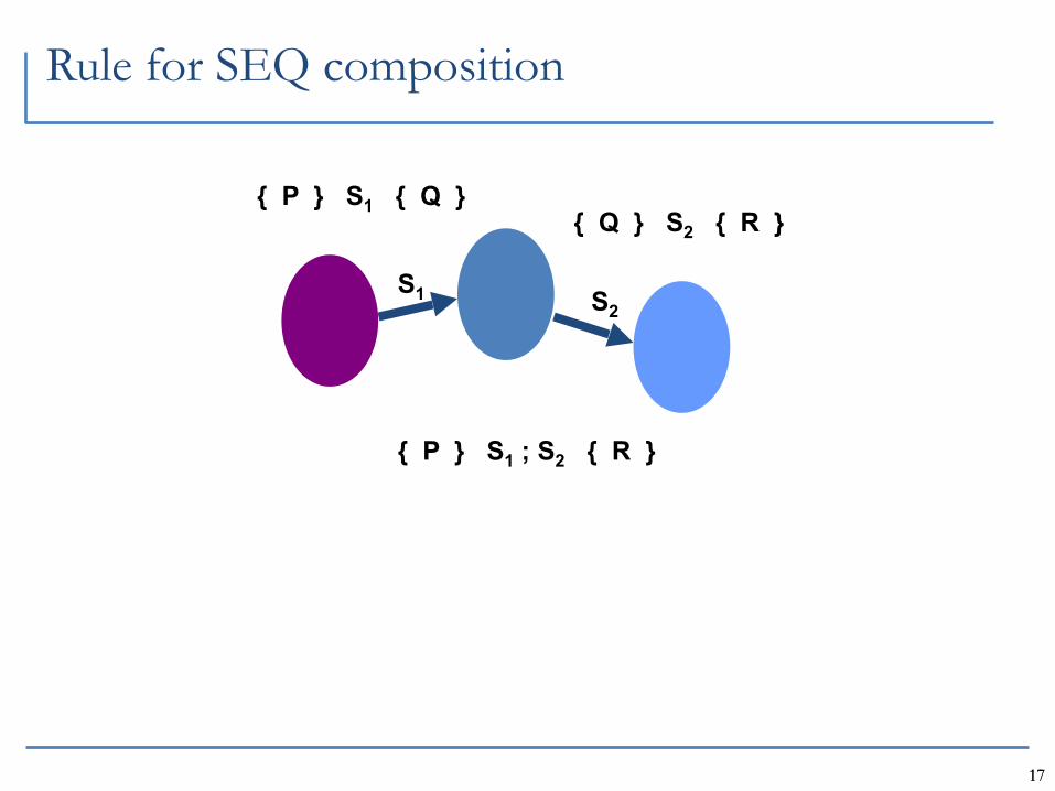
Rule for SEQ composition
{ P } S1 { Q }
S1
1616
Rule for SEQ composition
{ P } S1 { Q }{ Q } S2 { R }
S1 S2

1616
Rule for SEQ composition
{ P } S1 { Q }{ Q } S2 { R }
S1 S2
{ P } S1 ; S2 { R }
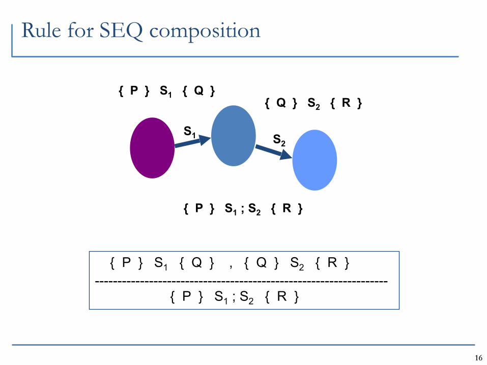
1616
Rule for SEQ composition
{ P } S1 { Q }{ Q } S2 { R }
S1 S2
{ P } S1 ; S2 { R }
{ P } S1 { Q } , { Q } S2 { R }----------------------------------------------------------------- { P } S1 ; S2 { R }
1717
Rule for SEQ composition
{ P } S1 { Q }
S1

1717
Rule for SEQ composition
{ P } S1 { Q }{ Q } S2 { R }
S1 S2
1717
Rule for SEQ composition
{ P } S1 { Q }{ Q } S2 { R }
S1 S2
{ P } S1 ; S2 { R }

1717
Rule for SEQ composition
{ P } S1 { Q }{ Q } S2 { R }
S1 S2
{ P } S1 ; S2 { R }
{ P } S1 { Q } , { Q } S2 { R }----------------------------------------------------------------- { P } S1 ; S2 { R }
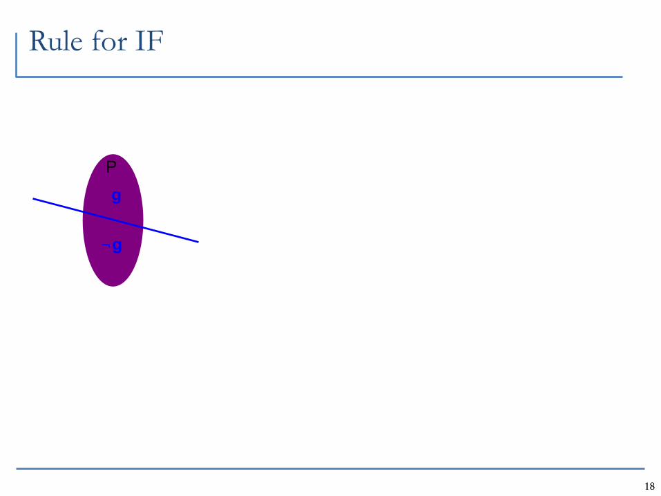
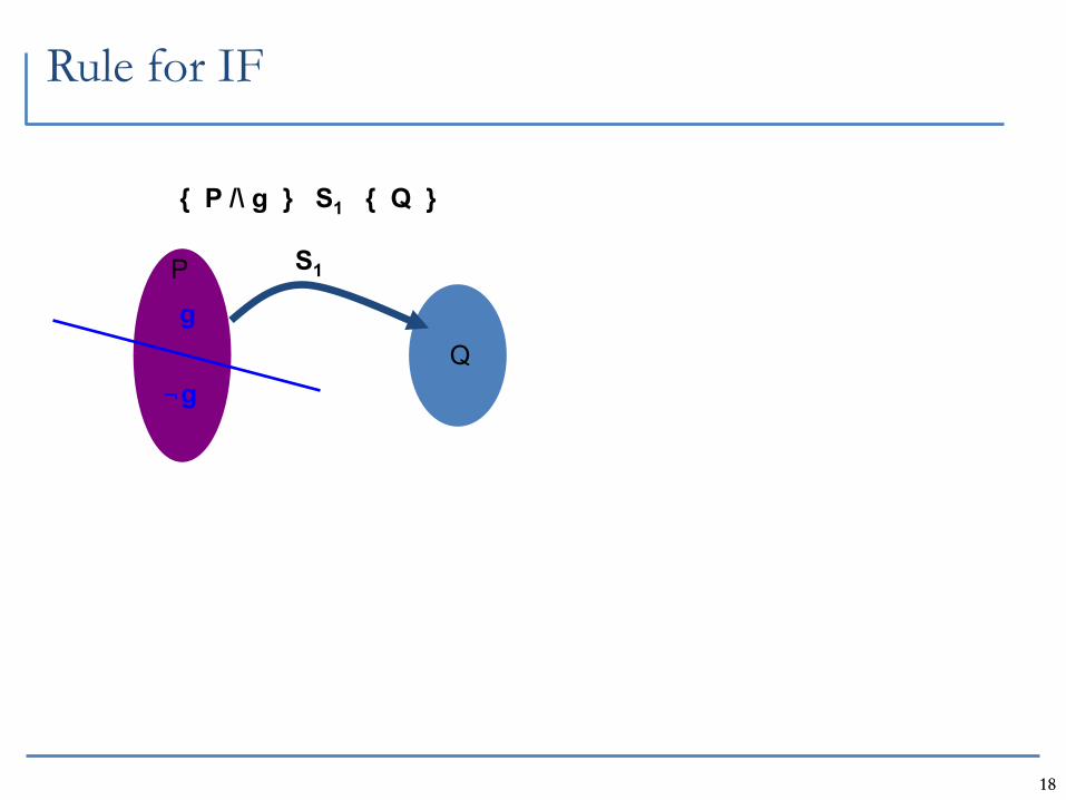
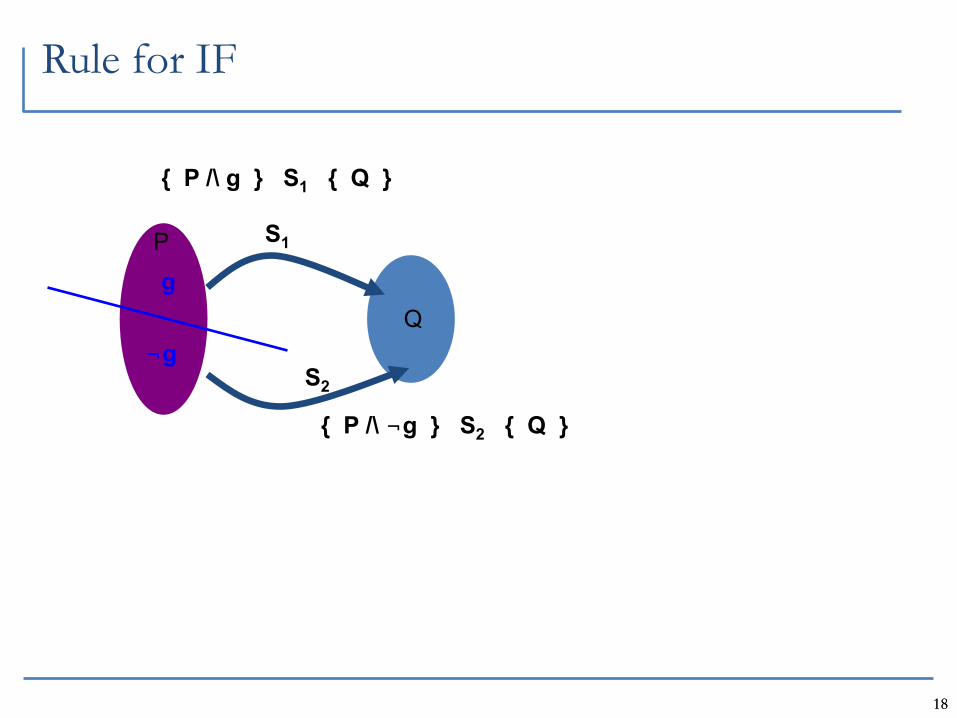
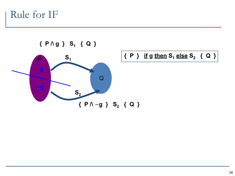
1818
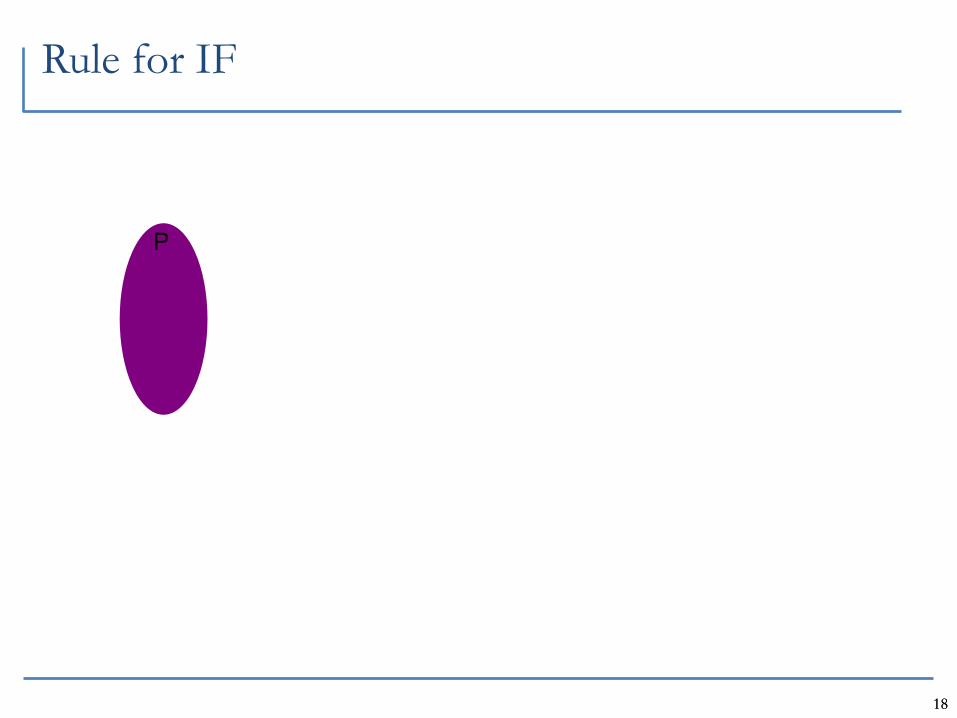
Rule for IF
P
1818
Rule for IF
g
¬g
P
1818
Rule for IF
{ P /\ g } S1 { Q }
Qg
¬g
S1P
1818
Rule for IF
{ P /\ g } S1 { Q }
Qg
¬g
S1P
S2
{ P /\ ¬g } S2 { Q }
1818
Rule for IF
{ P /\ g } S1 { Q }
Qg
¬g
S1P
S2
{ P /\ ¬g } S2 { Q }
{ P } if g then S1 else S2 { Q }
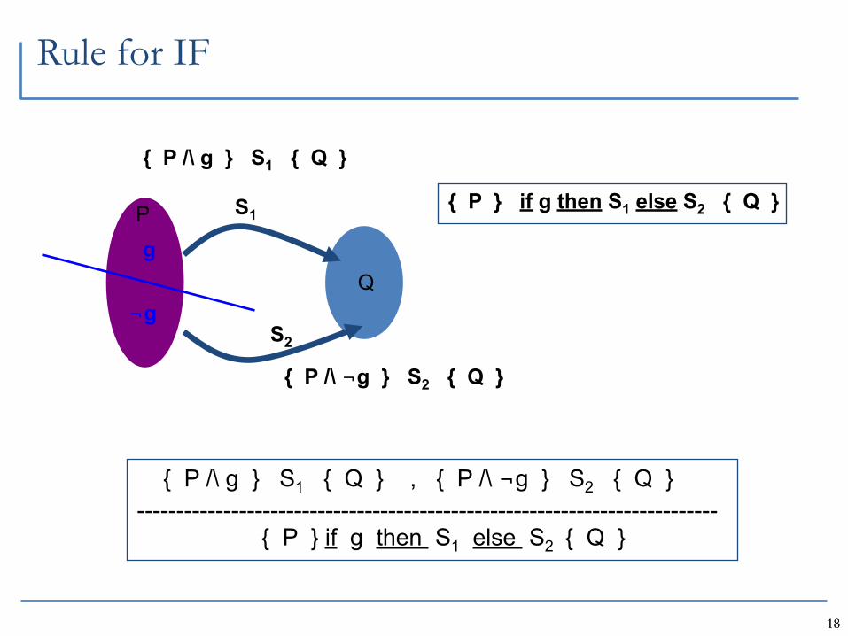
1818
Rule for IF
{ P /\ g } S1 { Q }
Qg
¬g
S1P
S2
{ P /\ ¬g } S2 { Q }
{ P } if g then S1 else S2 { Q }
{ P /\ g } S1 { Q } , { P /\ ¬g } S2 { Q }-------------------------------------------------------------------------- { P } if g then S1 else S2 { Q }
1919
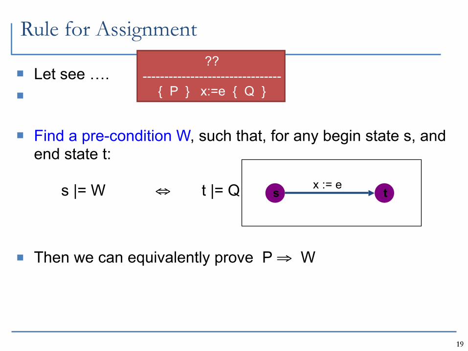
Rule for Assignment
Let see ….
Find a pre-condition W, such that, for any begin state s, and end state t:
s |= W ⇔ t |= Q
Then we can equivalently prove P ⇒ W
tsx := e
?? --------------------------------
{ P } x:=e { Q }
2020
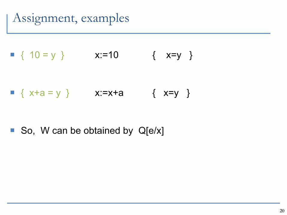
Assignment, examples
{ 10 = y } x:=10 { x=y }
{ x+a = y } x:=x+a { x=y }
So, W can be obtained by Q[e/x]
2121
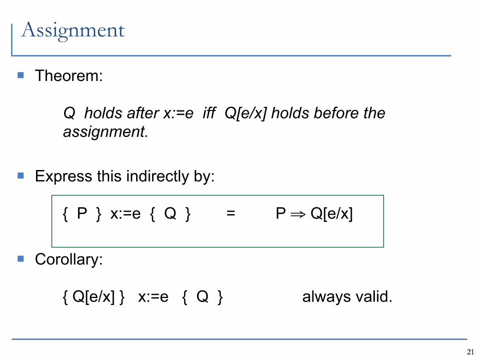
Assignment
Theorem:
Q holds after x:=e iff Q[e/x] holds before the assignment.
Express this indirectly by:
{ P } x:=e { Q } = P ⇒ Q[e/x]
Corollary:
{ Q[e/x] } x:=e { Q } always valid.
2222
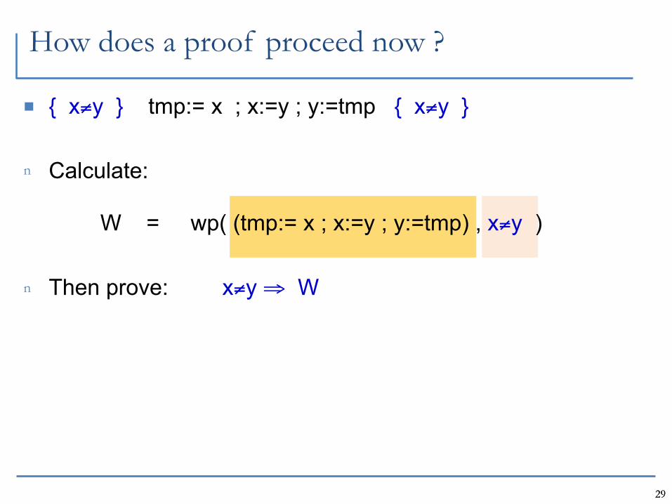
How does a proof proceed now ?
2222
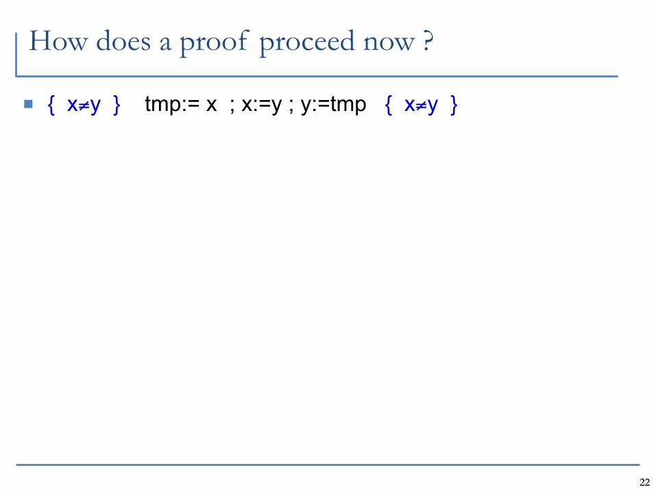
How does a proof proceed now ?
{ x≠y } tmp:= x ; x:=y ; y:=tmp { x≠y }
2222
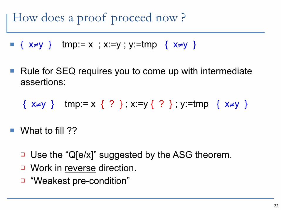
How does a proof proceed now ?
{ x≠y } tmp:= x ; x:=y ; y:=tmp { x≠y }
Rule for SEQ requires you to come up with intermediate assertions:
{ x≠y } tmp:= x { ? } ; x:=y { ? } ; y:=tmp { x≠y }
What to fill ??
Use the “Q[e/x]” suggested by the ASG theorem. Work in reverse direction. “Weakest pre-condition”
2323
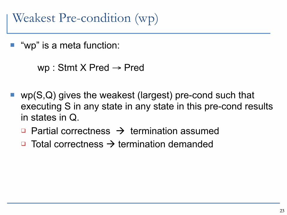
Weakest Pre-condition (wp)
“wp” is a meta function:
wp : Stmt X Pred → Pred
wp(S,Q) gives the weakest (largest) pre-cond such that executing S in any state in any state in this pre-cond results in states in Q. Partial correctness termination assumed Total correctness termination demanded
2424
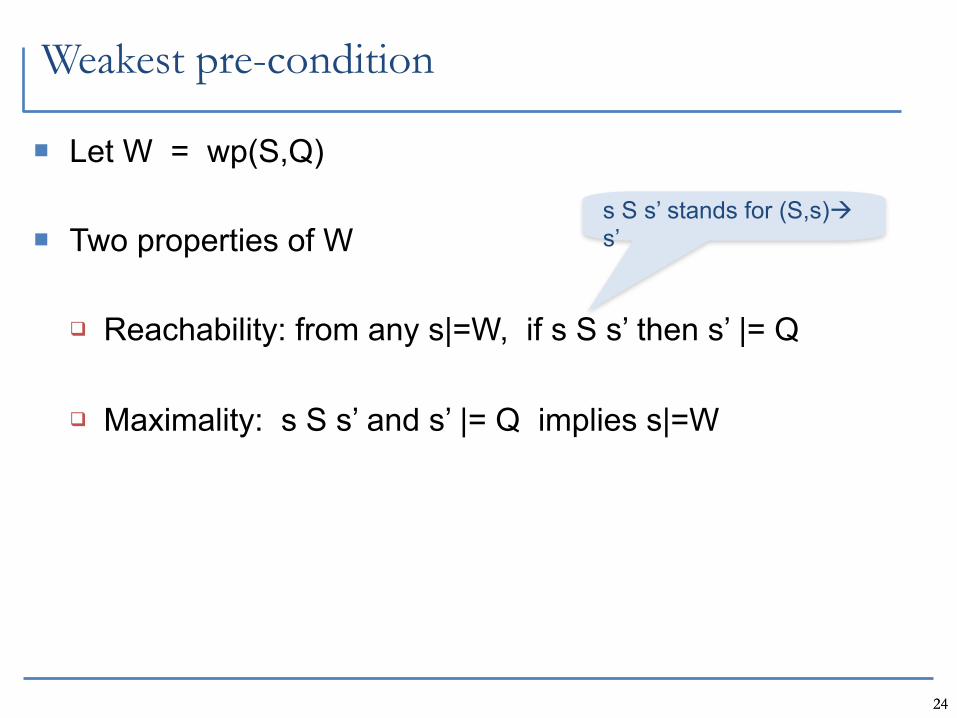
Weakest pre-condition
Let W = wp(S,Q)
Two properties of W
Reachability: from any s|=W, if s S s’ then s’ |= Q
Maximality: s S s’ and s’ |= Q implies s|=W
s S s’ stands for (S,s) s’
2525
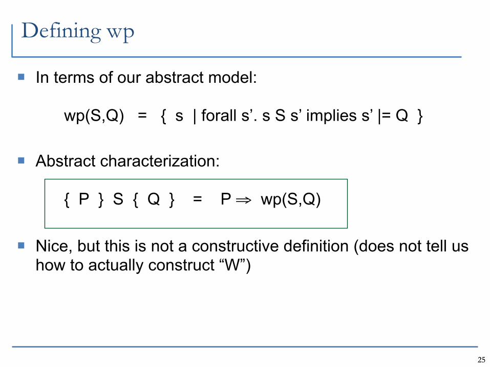
Defining wp
In terms of our abstract model:
wp(S,Q) = { s | forall s’. s S s’ implies s’ |= Q }
Abstract characterization:
{ P } S { Q } = P ⇒ wp(S,Q)
Nice, but this is not a constructive definition (does not tell us how to actually construct “W”)
2626
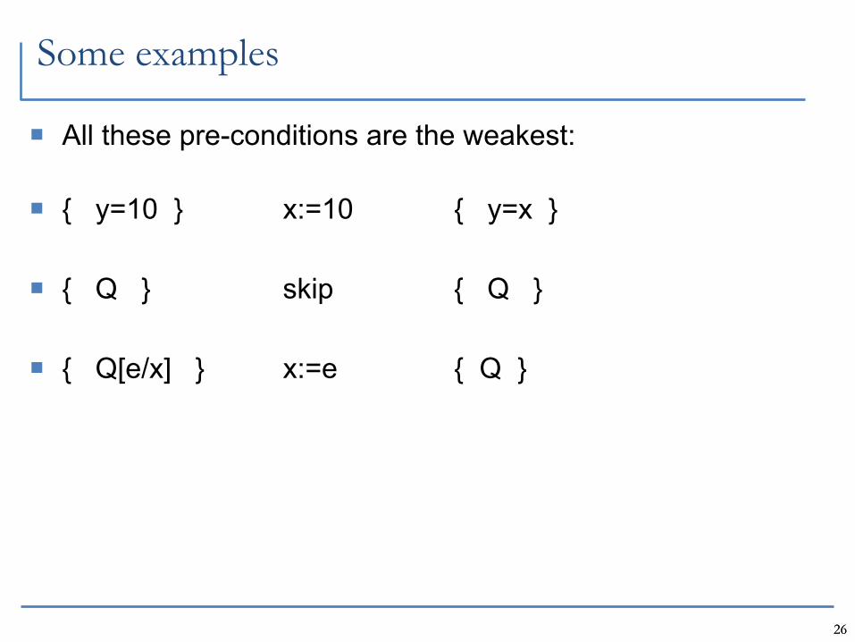
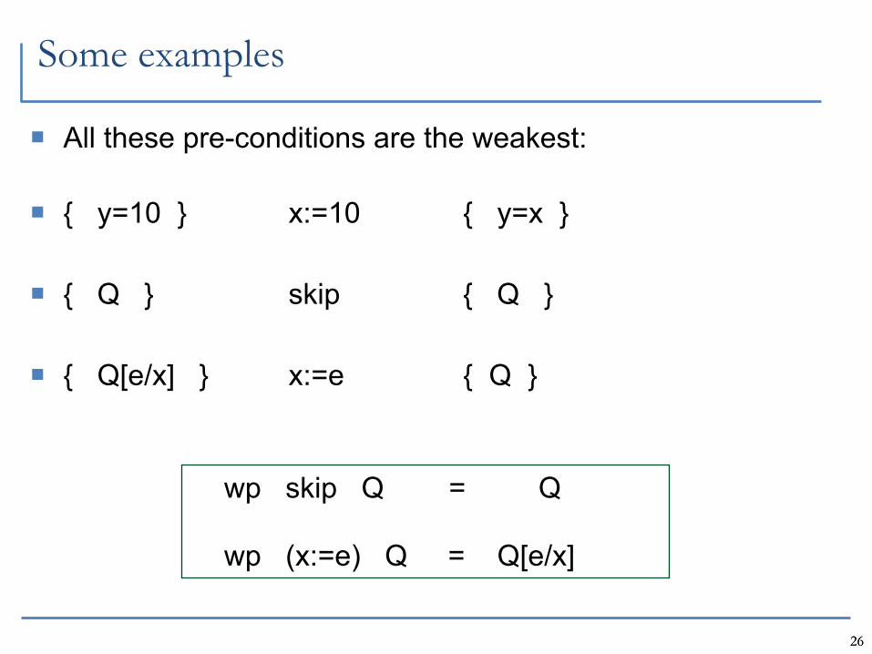
Some examples
All these pre-conditions are the weakest:
{ y=10 } x:=10 { y=x }
{ Q } skip { Q }
{ Q[e/x] } x:=e { Q }
2626
Some examples
All these pre-conditions are the weakest:
{ y=10 } x:=10 { y=x }
{ Q } skip { Q }
{ Q[e/x] } x:=e { Q }
wp skip Q = Q
wp (x:=e) Q = Q[e/x]
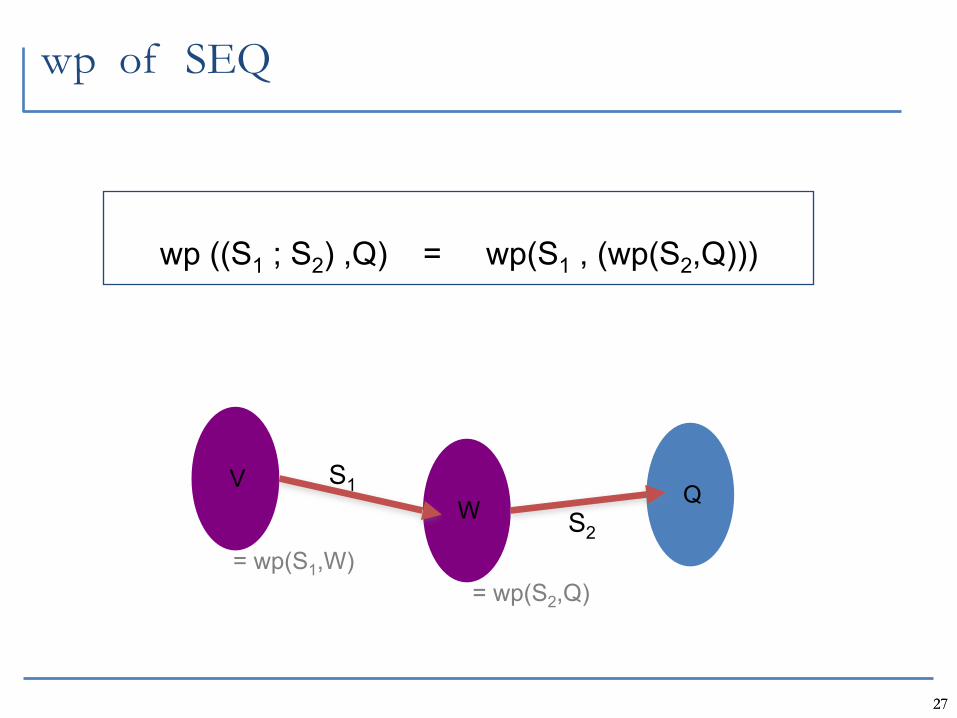
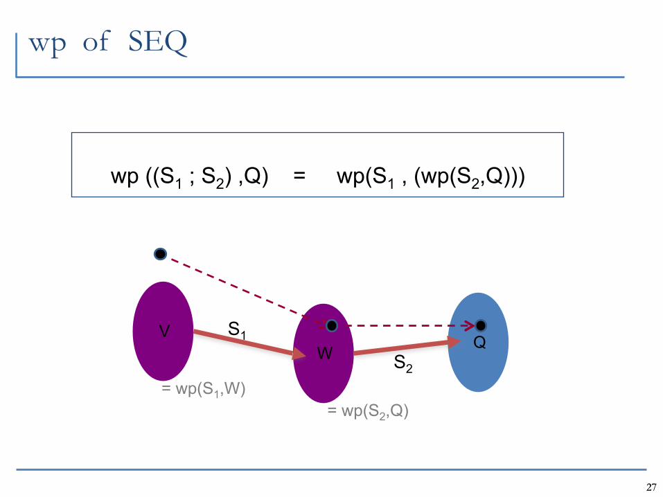
2727
wp of SEQ
wp ((S1 ; S2) ,Q) = wp(S1 , (wp(S2,Q)))
QW
= wp(S2,Q)
V
= wp(S1,W)S2
S1
2727
wp of SEQ
wp ((S1 ; S2) ,Q) = wp(S1 , (wp(S2,Q)))
QW
= wp(S2,Q)
V
= wp(S1,W)S2
S1

2727
wp of SEQ
wp ((S1 ; S2) ,Q) = wp(S1 , (wp(S2,Q)))
QW
= wp(S2,Q)
V
= wp(S1,W)S2
S1
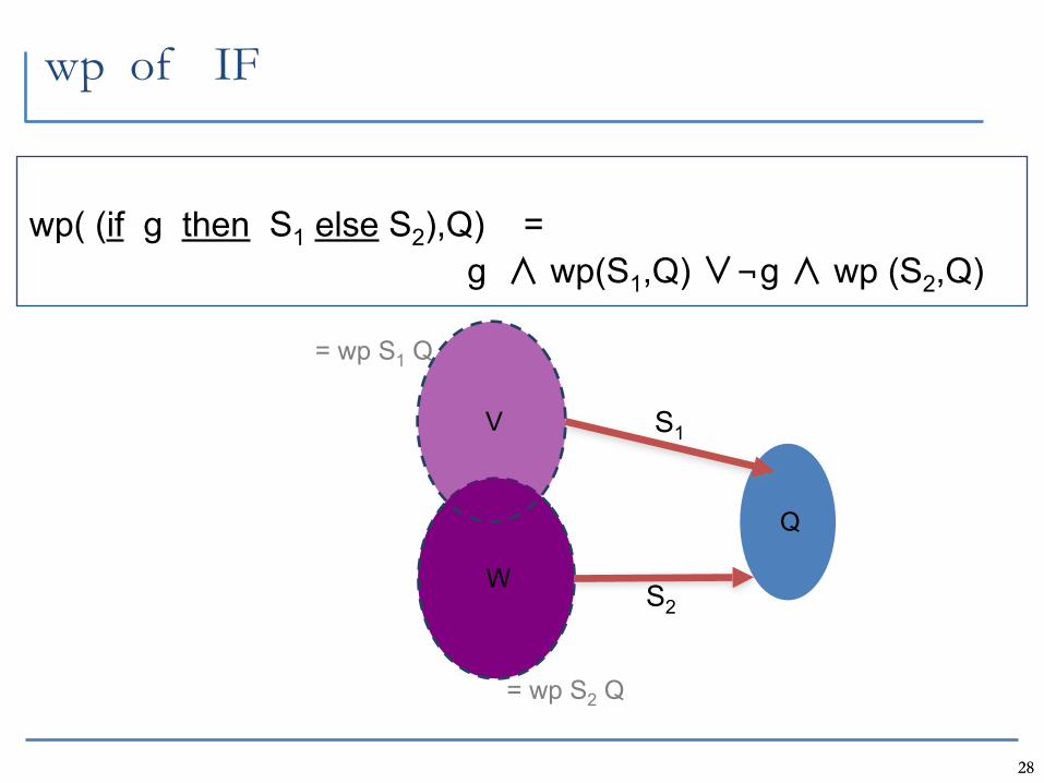
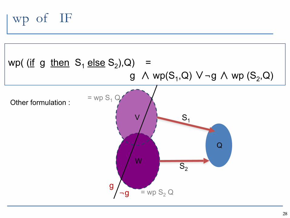
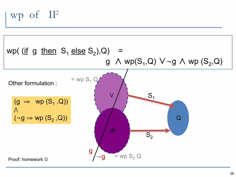
2828
wp of IF
wp( (if g then S1 else S2),Q) =
g ∧ wp(S1,Q) ∨¬g ∧ wp (S2,Q)
Q
W
= wp S2 Q
V
= wp S1 Q
S2
S1

2828
wp of IF
wp( (if g then S1 else S2),Q) =
g ∧ wp(S1,Q) ∨¬g ∧ wp (S2,Q)
Q
W
= wp S2 Q
V
= wp S1 Q
S2
S1
g¬g
2828
wp of IF
wp( (if g then S1 else S2),Q) =
g ∧ wp(S1,Q) ∨¬g ∧ wp (S2,Q)
Q
W
= wp S2 Q
V
= wp S1 Q
S2
S1
g¬g
Other formulation :
2828
wp of IF
wp( (if g then S1 else S2),Q) =
g ∧ wp(S1,Q) ∨¬g ∧ wp (S2,Q)
Q
W
= wp S2 Q
V
= wp S1 Q
S2
S1
g¬g
(g ⇒ wp (S1 ,Q))/\(¬g ⇒ wp (S2 ,Q))
Other formulation :
Proof: homework
2929
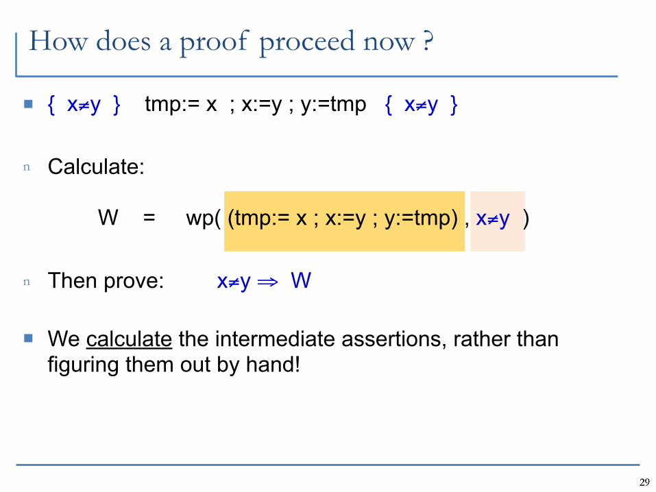
How does a proof proceed now ?
2929
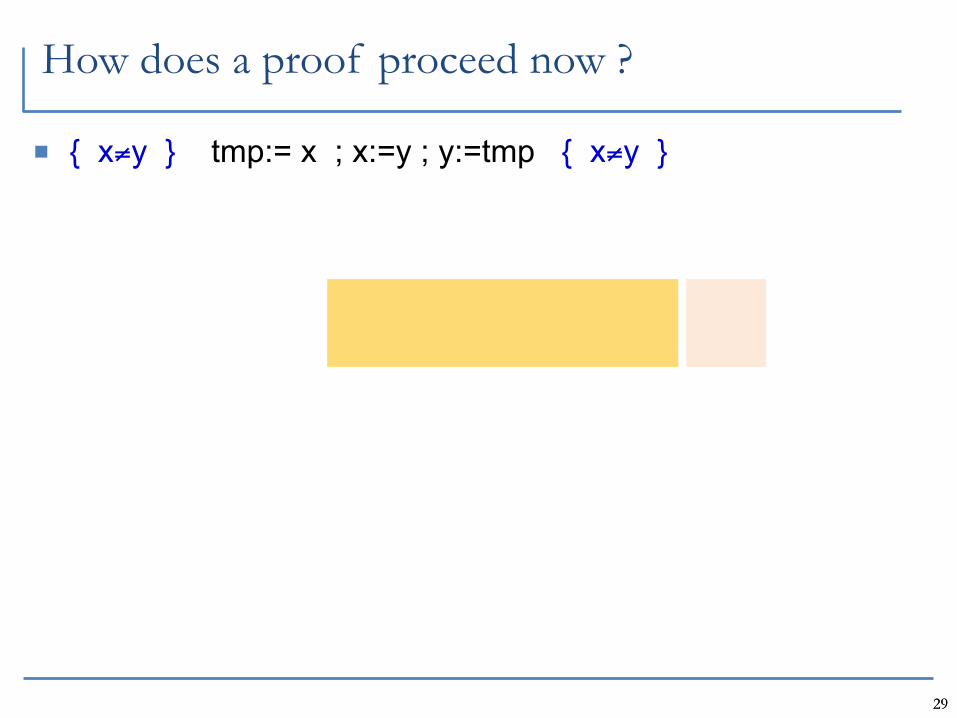
How does a proof proceed now ?
{ x≠y } tmp:= x ; x:=y ; y:=tmp { x≠y }

2929
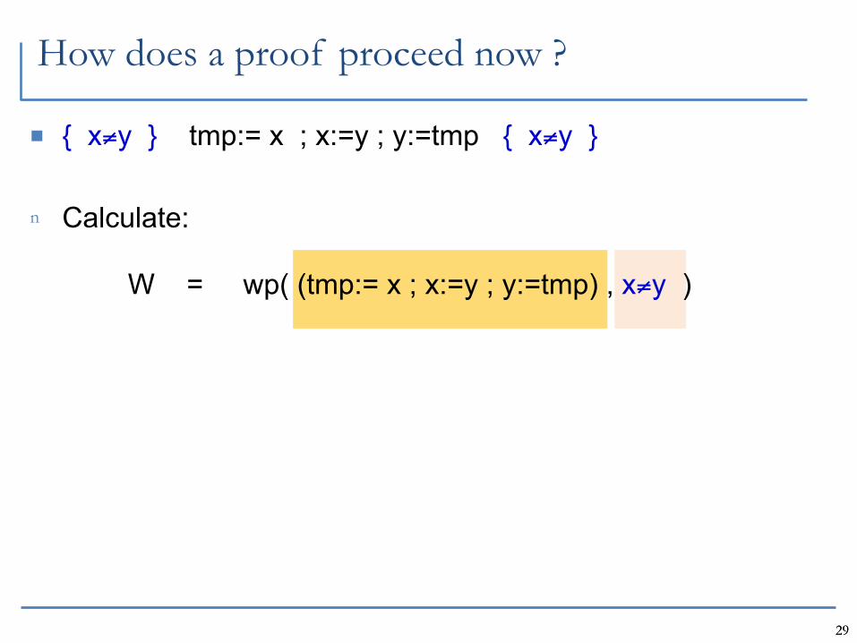
How does a proof proceed now ?
{ x≠y } tmp:= x ; x:=y ; y:=tmp { x≠y }
n Calculate:
W = wp( (tmp:= x ; x:=y ; y:=tmp) , x≠y )
2929
How does a proof proceed now ?
{ x≠y } tmp:= x ; x:=y ; y:=tmp { x≠y }
n Calculate:
W = wp( (tmp:= x ; x:=y ; y:=tmp) , x≠y )
2929
How does a proof proceed now ?
{ x≠y } tmp:= x ; x:=y ; y:=tmp { x≠y }
n Calculate:
W = wp( (tmp:= x ; x:=y ; y:=tmp) , x≠y )
n Then prove: x≠y ⇒ W
2929
How does a proof proceed now ?
{ x≠y } tmp:= x ; x:=y ; y:=tmp { x≠y }
n Calculate:
W = wp( (tmp:= x ; x:=y ; y:=tmp) , x≠y )
n Then prove: x≠y ⇒ W
We calculate the intermediate assertions, rather than figuring them out by hand!
30
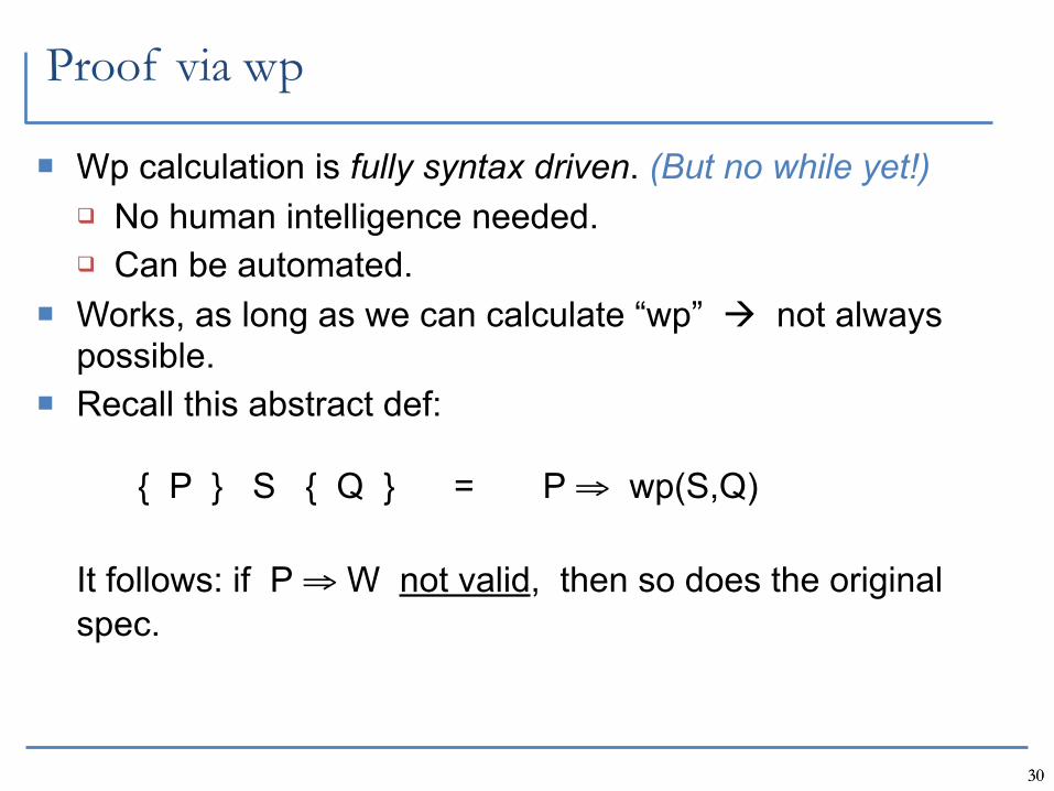
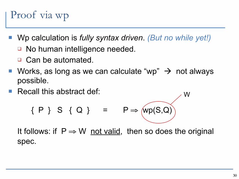
Proof via wp
Wp calculation is fully syntax driven. (But no while yet!) No human intelligence needed. Can be automated.
Works, as long as we can calculate “wp” not always possible.
Recall this abstract def:
{ P } S { Q } = P ⇒ wp(S,Q)
It follows: if P ⇒ W not valid, then so does the original spec.
30
30
Proof via wp
Wp calculation is fully syntax driven. (But no while yet!) No human intelligence needed. Can be automated.
Works, as long as we can calculate “wp” not always possible.
Recall this abstract def:
{ P } S { Q } = P ⇒ wp(S,Q)
It follows: if P ⇒ W not valid, then so does the original spec.
30
W
31
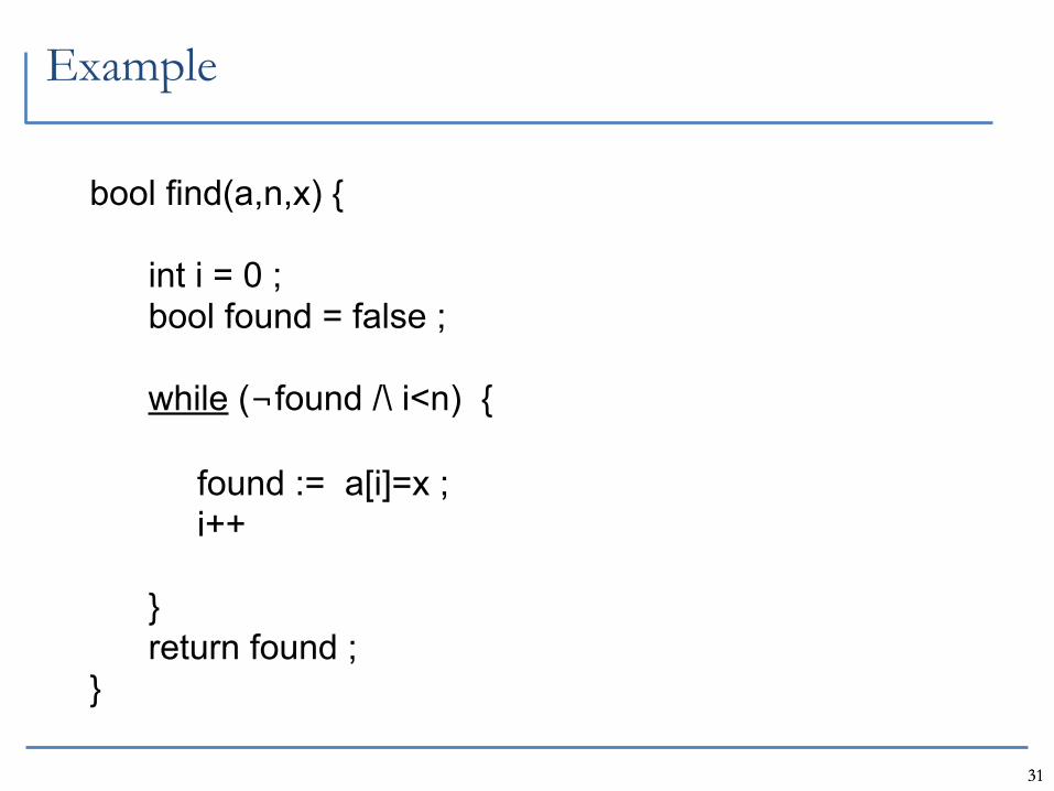
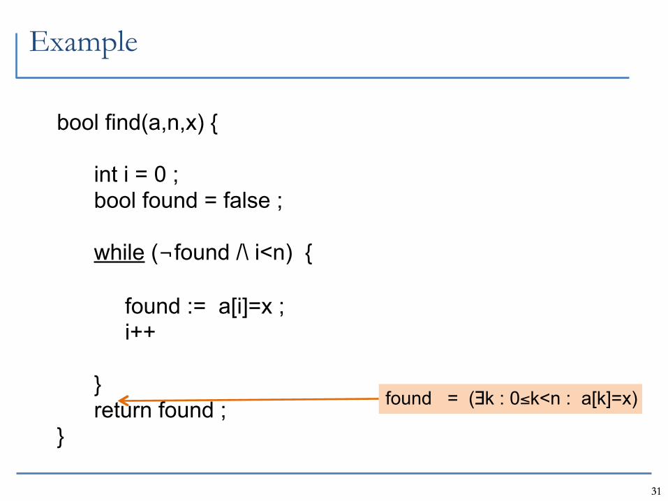
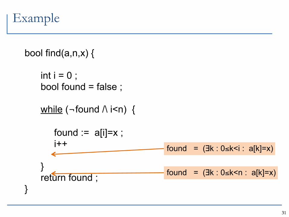
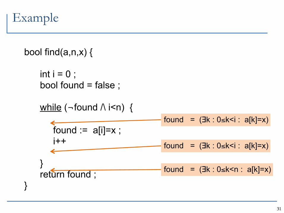
Example
31
bool find(a,n,x) {
int i = 0 ; bool found = false ;
while (¬found /\ i<n) {
found := a[i]=x ; i++
} return found ; }
31
Example
31
bool find(a,n,x) {
int i = 0 ; bool found = false ;
while (¬found /\ i<n) {
found := a[i]=x ; i++
} return found ; }
found = (∃k : 0≤k<n : a[k]=x)

31
Example
31
bool find(a,n,x) {
int i = 0 ; bool found = false ;
while (¬found /\ i<n) {
found := a[i]=x ; i++
} return found ; }
found = (∃k : 0≤k<n : a[k]=x)
found = (∃k : 0≤k<i : a[k]=x)

31
Example
31
bool find(a,n,x) {
int i = 0 ; bool found = false ;
while (¬found /\ i<n) {
found := a[i]=x ; i++
} return found ; }
found = (∃k : 0≤k<n : a[k]=x)
found = (∃k : 0≤k<i : a[k]=x)
31
Example
31
bool find(a,n,x) {
int i = 0 ; bool found = false ;
while (¬found /\ i<n) {
found := a[i]=x ; i++
} return found ; }
found = (∃k : 0≤k<n : a[k]=x)
found = (∃k : 0≤k<i : a[k]=x)
31
Example
31
bool find(a,n,x) {
int i = 0 ; bool found = false ;
while (¬found /\ i<n) {
found := a[i]=x ; i++
} return found ; }
found = (∃k : 0≤k<n : a[k]=x)
found = (∃k : 0≤k<i : a[k]=x)
found = (∃k : 0≤k<i : a[k]=x)

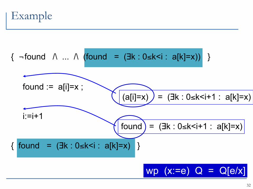
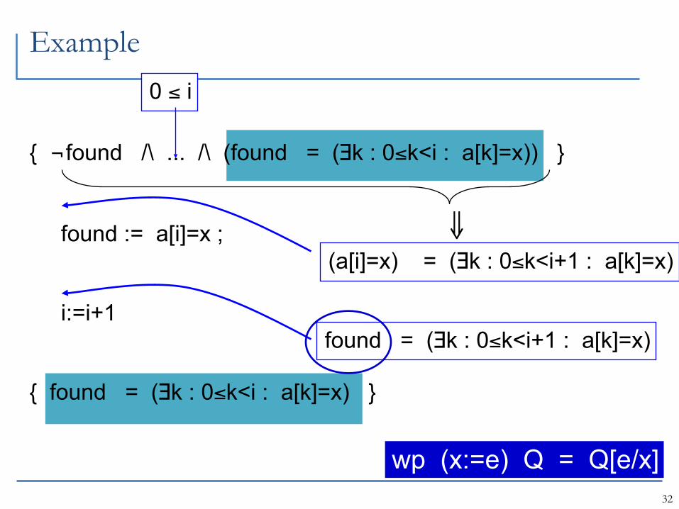
32
Example
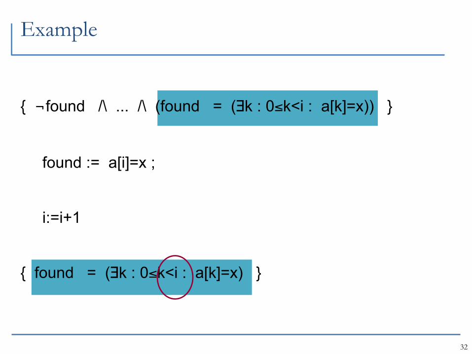
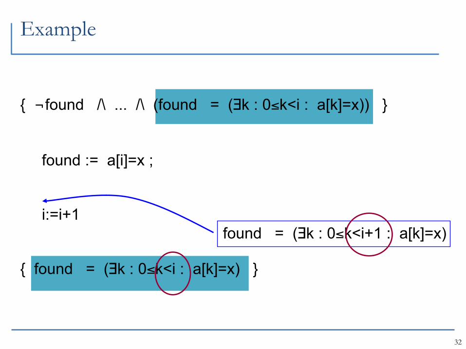
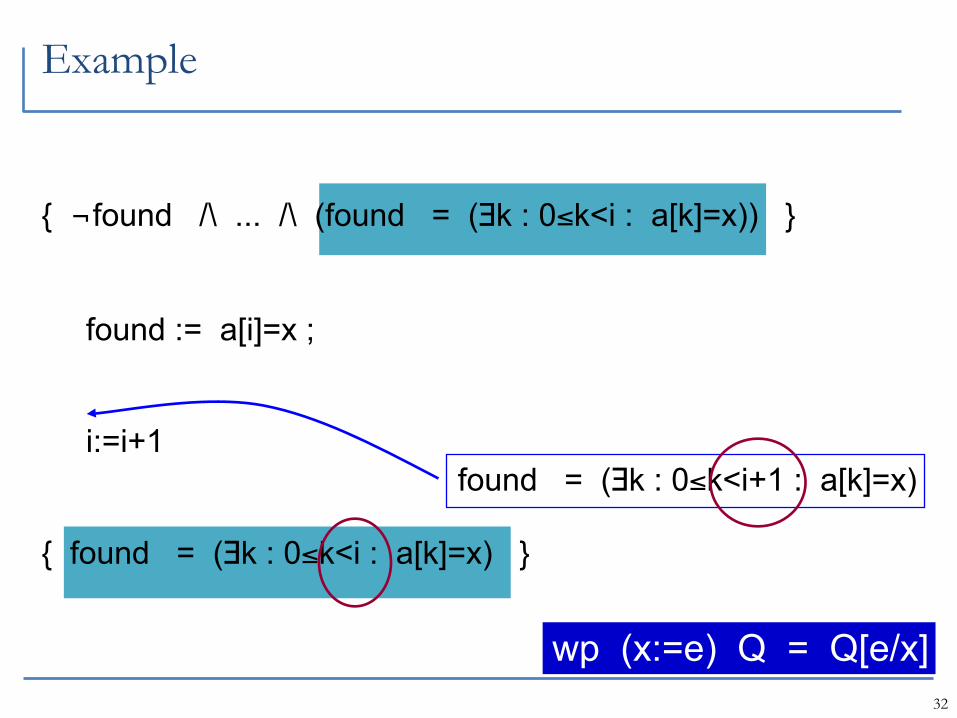
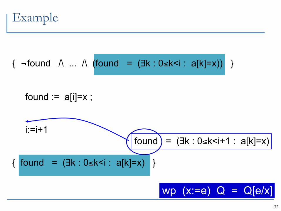
{ ¬found /\ ... /\ (found = (∃k : 0≤k<i : a[k]=x)) }
found := a[i]=x ;
i:=i+1
{ found = (∃k : 0≤k<i : a[k]=x) }
32
Example
{ ¬found /\ ... /\ (found = (∃k : 0≤k<i : a[k]=x)) }
found := a[i]=x ;
i:=i+1
{ found = (∃k : 0≤k<i : a[k]=x) }
32
Example
{ ¬found /\ ... /\ (found = (∃k : 0≤k<i : a[k]=x)) }
found := a[i]=x ;
i:=i+1
{ found = (∃k : 0≤k<i : a[k]=x) }
found = (∃k : 0≤k<i+1 : a[k]=x)
32
Example
{ ¬found /\ ... /\ (found = (∃k : 0≤k<i : a[k]=x)) }
found := a[i]=x ;
i:=i+1
{ found = (∃k : 0≤k<i : a[k]=x) }
found = (∃k : 0≤k<i+1 : a[k]=x)
wp (x:=e) Q = Q[e/x]
32
Example
{ ¬found /\ ... /\ (found = (∃k : 0≤k<i : a[k]=x)) }
found := a[i]=x ;
i:=i+1
{ found = (∃k : 0≤k<i : a[k]=x) }
found = (∃k : 0≤k<i+1 : a[k]=x)
wp (x:=e) Q = Q[e/x]
32
Example
{ ¬found /\ ... /\ (found = (∃k : 0≤k<i : a[k]=x)) }
found := a[i]=x ;
i:=i+1
{ found = (∃k : 0≤k<i : a[k]=x) }
found = (∃k : 0≤k<i+1 : a[k]=x)
(a[i]=x) = (∃k : 0≤k<i+1 : a[k]=x)
wp (x:=e) Q = Q[e/x]

32
Example
{ ¬found /\ ... /\ (found = (∃k : 0≤k<i : a[k]=x)) }
found := a[i]=x ;
i:=i+1
{ found = (∃k : 0≤k<i : a[k]=x) }
found = (∃k : 0≤k<i+1 : a[k]=x)
(a[i]=x) = (∃k : 0≤k<i+1 : a[k]=x)
wp (x:=e) Q = Q[e/x]
⇒
32
Example
{ ¬found /\ ... /\ (found = (∃k : 0≤k<i : a[k]=x)) }
found := a[i]=x ;
i:=i+1
{ found = (∃k : 0≤k<i : a[k]=x) }
found = (∃k : 0≤k<i+1 : a[k]=x)
(a[i]=x) = (∃k : 0≤k<i+1 : a[k]=x)
0 ≤ i
wp (x:=e) Q = Q[e/x]
⇒
Reasoning about loops
33
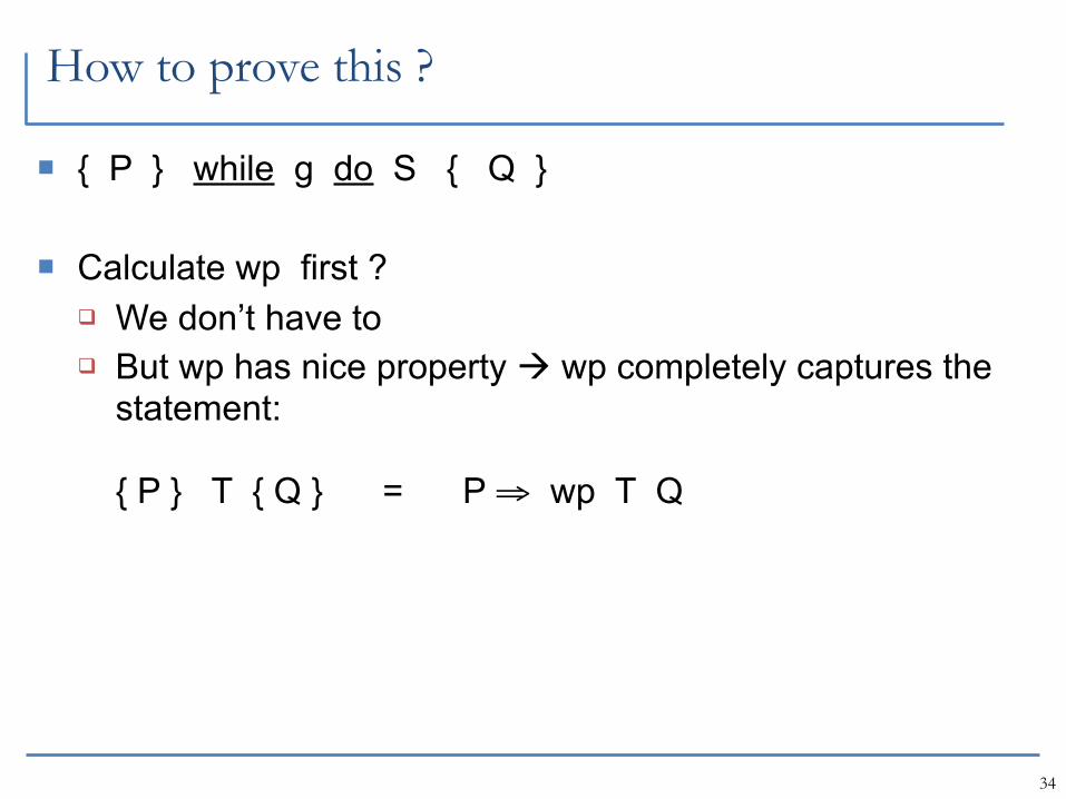
How to prove this ?
{ P } while g do S { Q }
Calculate wp first ? We don’t have to But wp has nice property wp completely captures the
statement:
{ P } T { Q } = P ⇒ wp T Q
34
wp of a loop ….
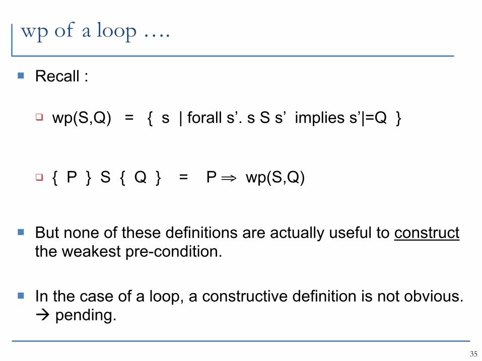
Recall :
wp(S,Q) = { s | forall s’. s S s’ implies s’|=Q }
{ P } S { Q } = P ⇒ wp(S,Q)
But none of these definitions are actually useful to construct the weakest pre-condition.
In the case of a loop, a constructive definition is not obvious. pending.
35
How to prove this ?
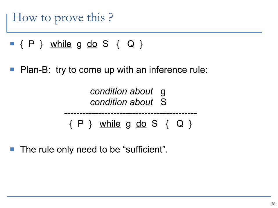
{ P } while g do S { Q }
Plan-B: try to come up with an inference rule:
condition about g condition about S ------------------------------------------- { P } while g do S { Q }
The rule only need to be “sufficient”.
36
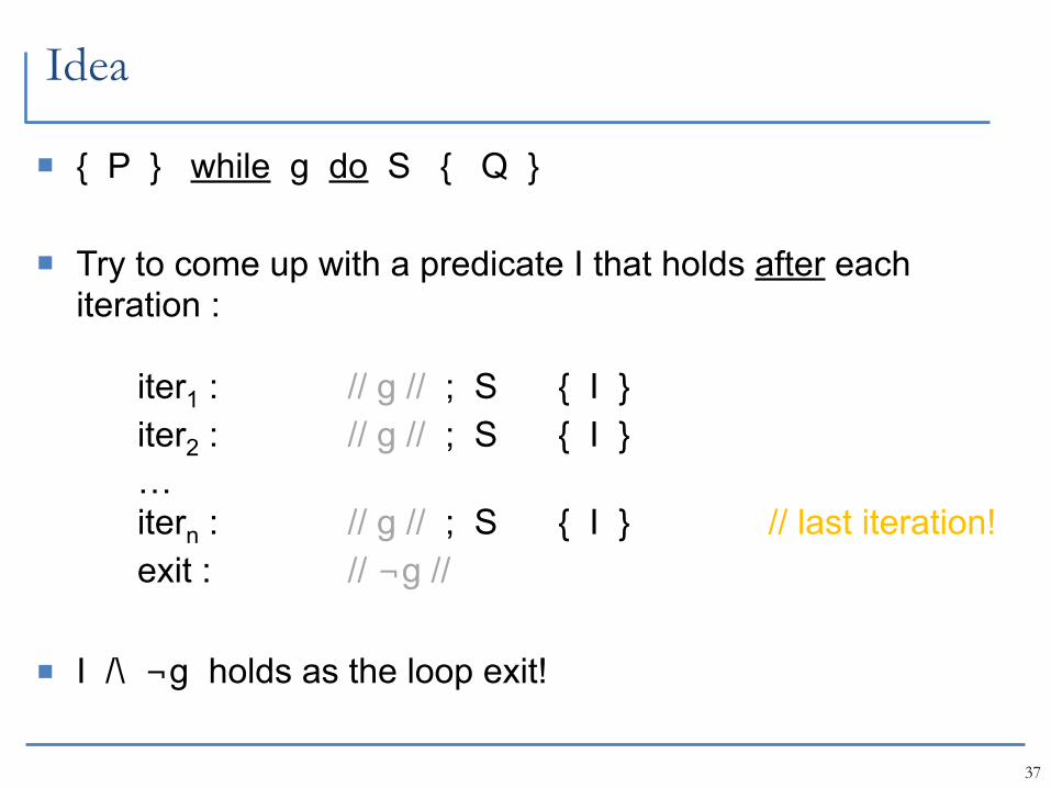
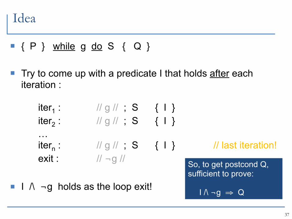
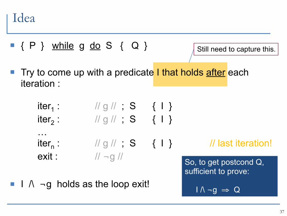
Idea
37

Idea
{ P } while g do S { Q }
37
Idea
{ P } while g do S { Q }
37
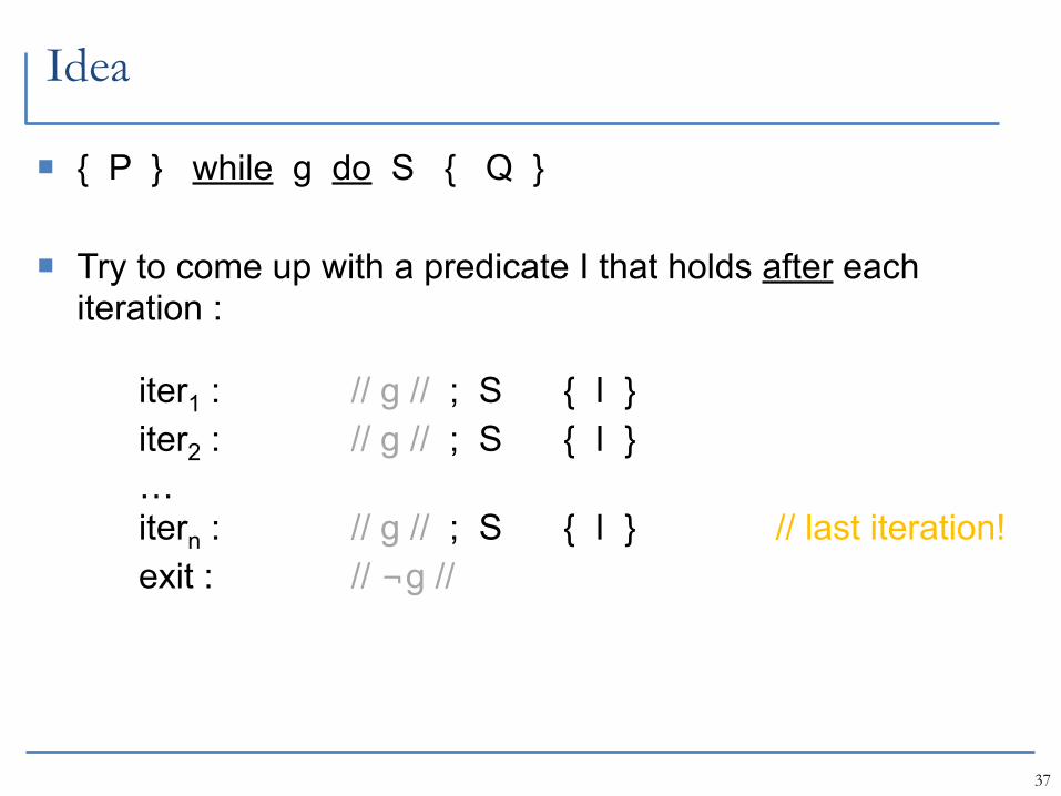
Idea
{ P } while g do S { Q }
Try to come up with a predicate I that holds after each iteration :
iter1 : // g // ; S { I } iter2 : // g // ; S { I } … itern : // g // ; S { I } // last iteration! exit : // ¬g //
37

Idea
{ P } while g do S { Q }
Try to come up with a predicate I that holds after each iteration :
iter1 : // g // ; S { I } iter2 : // g // ; S { I } … itern : // g // ; S { I } // last iteration! exit : // ¬g //
37
Idea
{ P } while g do S { Q }
Try to come up with a predicate I that holds after each iteration :
iter1 : // g // ; S { I } iter2 : // g // ; S { I } … itern : // g // ; S { I } // last iteration! exit : // ¬g //
I /\ ¬g holds as the loop exit!
37
Idea
{ P } while g do S { Q }
Try to come up with a predicate I that holds after each iteration :
iter1 : // g // ; S { I } iter2 : // g // ; S { I } … itern : // g // ; S { I } // last iteration! exit : // ¬g //
I /\ ¬g holds as the loop exit!
37
So, to get postcond Q, sufficient to prove:
I /\ ¬g ⇒ Q
Still need to capture this.
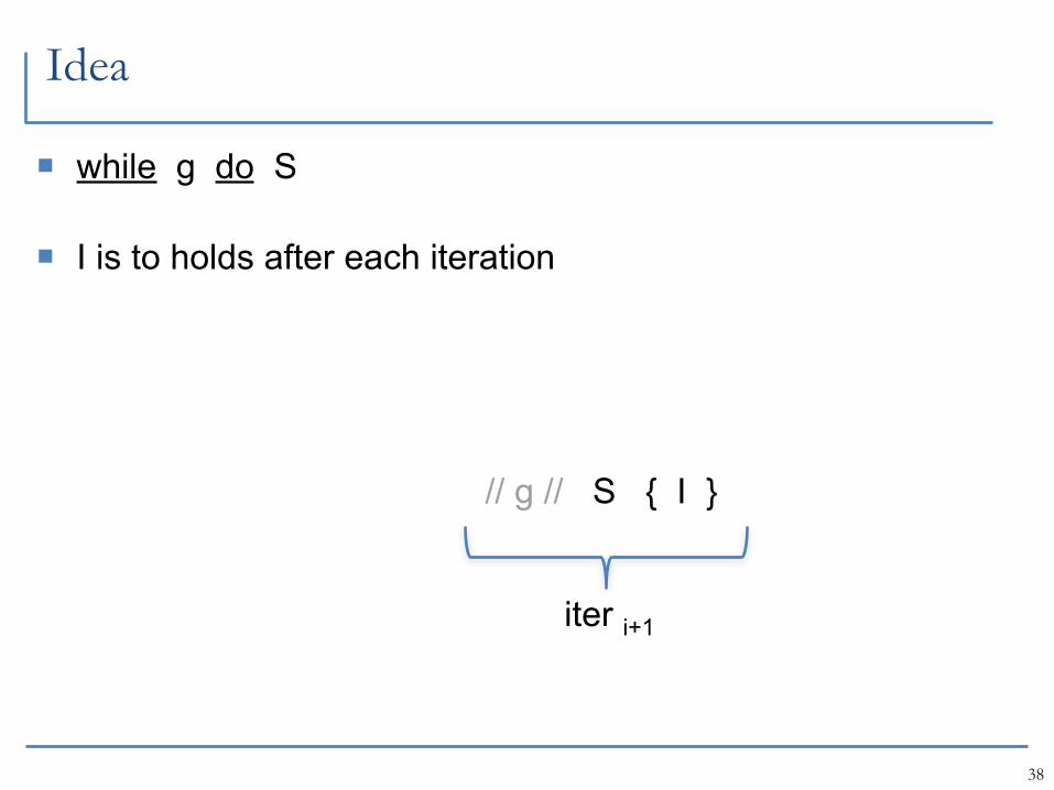
Idea
while g do S
I is to holds after each iteration
38
// g // S { I }
iter i+1
Idea
while g do S
I is to holds after each iteration
38
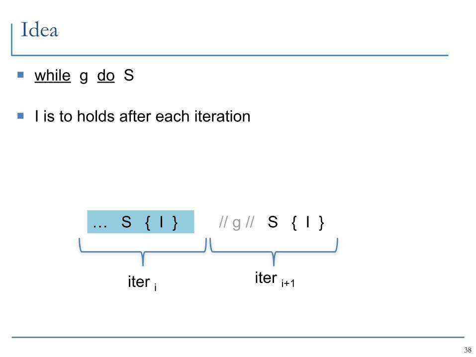
… S { I } // g // S { I }
iter i+1iter i
Idea
while g do S
I is to holds after each iteration
38
… S { I } // g // S { I }
iter i+1iter i
Idea
while g do S
I is to holds after each iteration
38
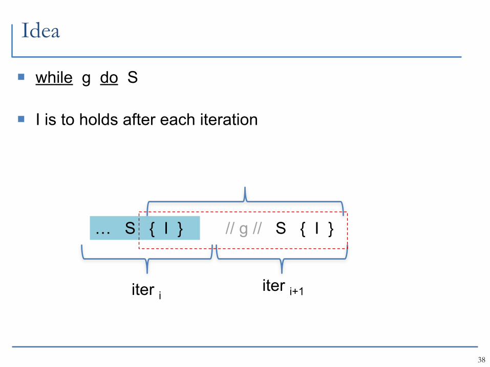
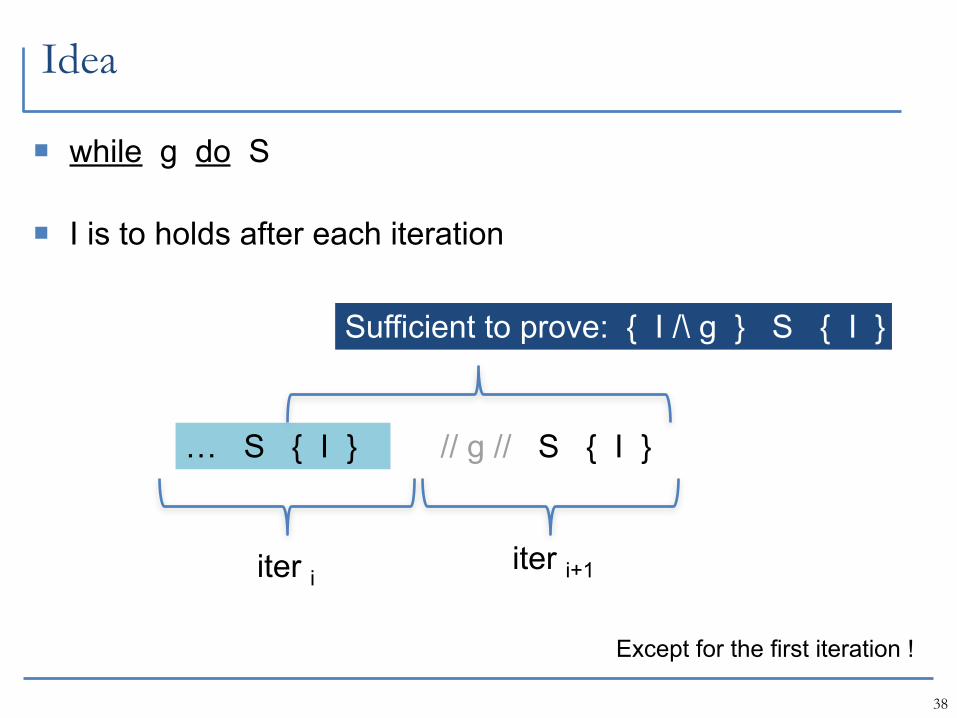
… S { I } // g // S { I }
iter i+1iter i
Sufficient to prove: { I /\ g } S { I }
Except for the first iteration !
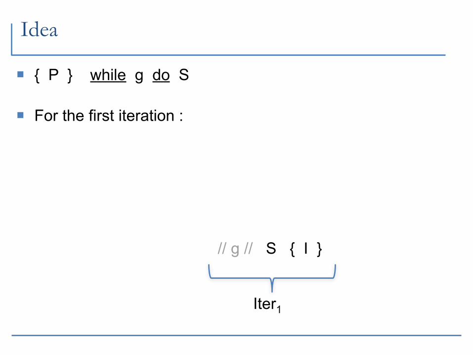
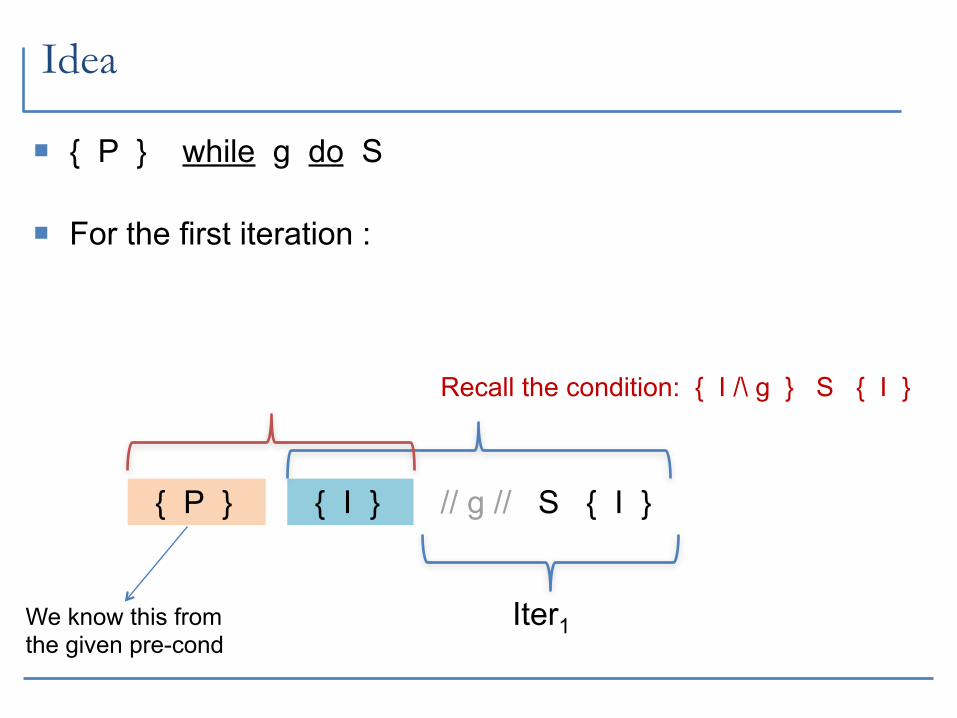
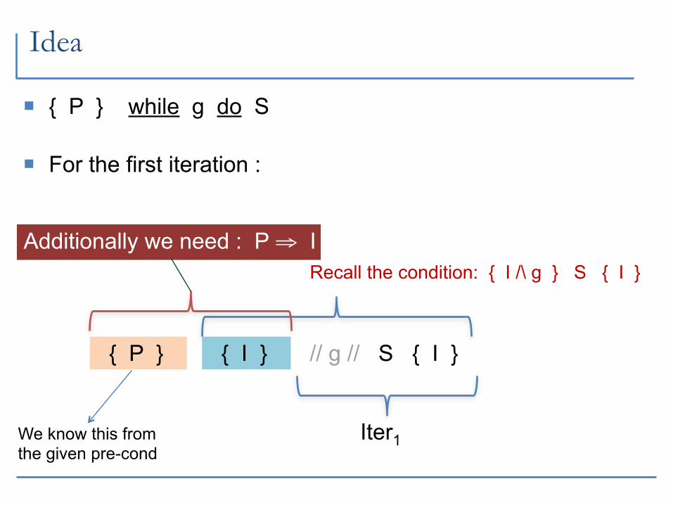
Idea
{ P } while g do S
For the first iteration :
// g // S { I }
Iter1
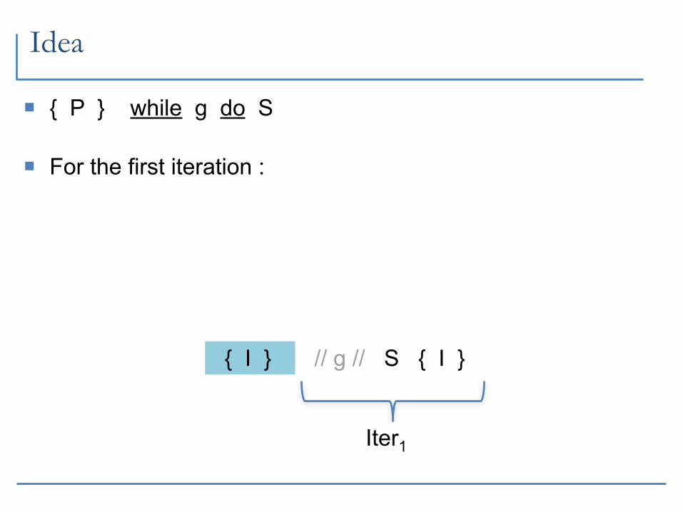
Idea
{ P } while g do S
For the first iteration :
{ I } // g // S { I }
Iter1
Idea
{ P } while g do S
For the first iteration :
{ I } // g // S { I }
Iter1
Recall the condition: { I /\ g } S { I }
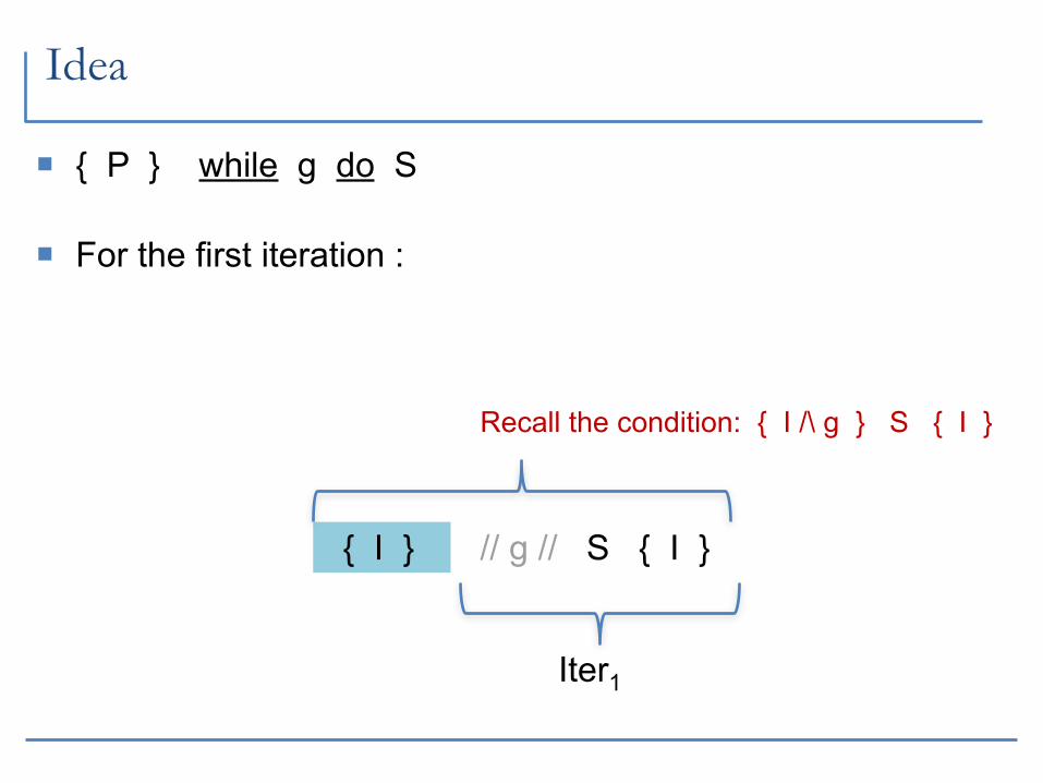
Idea
{ P } while g do S
For the first iteration :
{ I } // g // S { I }
Iter1We know this from the given pre-cond
Recall the condition: { I /\ g } S { I }
{ P }
Idea
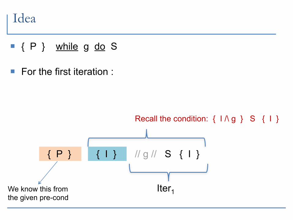
{ P } while g do S
For the first iteration :
{ I } // g // S { I }
Iter1We know this from the given pre-cond
Recall the condition: { I /\ g } S { I }
{ P }
Idea
{ P } while g do S
For the first iteration :
{ I } // g // S { I }
Iter1We know this from the given pre-cond
Recall the condition: { I /\ g } S { I }
{ P }
Additionally we need : P ⇒ I
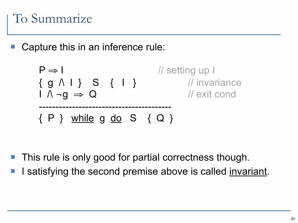
To Summarize
Capture this in an inference rule:
P ⇒ I // setting up I { g /\ I } S { I } // invariance I /\ ¬g ⇒ Q // exit cond ---------------------------------------- { P } while g do S { Q }
This rule is only good for partial correctness though. I satisfying the second premise above is called invariant.
40
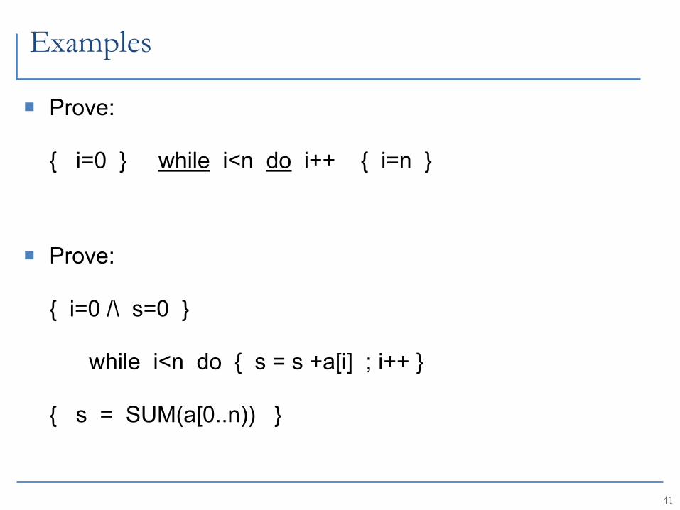
Examples
Prove:
{ i=0 } while i<n do i++ { i=n }
Prove:
{ i=0 /\ s=0 }
while i<n do { s = s +a[i] ; i++ }
{ s = SUM(a[0..n)) }
41
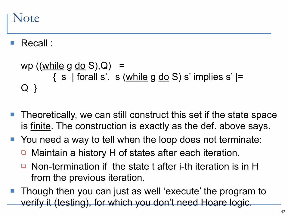
Note
Recall :
wp ((while g do S),Q) = { s | forall s’. s (while g do S) s’ implies s’ |= Q }
Theoretically, we can still construct this set if the state space is finite. The construction is exactly as the def. above says.
You need a way to tell when the loop does not terminate: Maintain a history H of states after each iteration. Non-termination if the state t after i-th iteration is in H
from the previous iteration. Though then you can just as well ‘execute’ the program to
verify it (testing), for which you don’t need Hoare logic.42
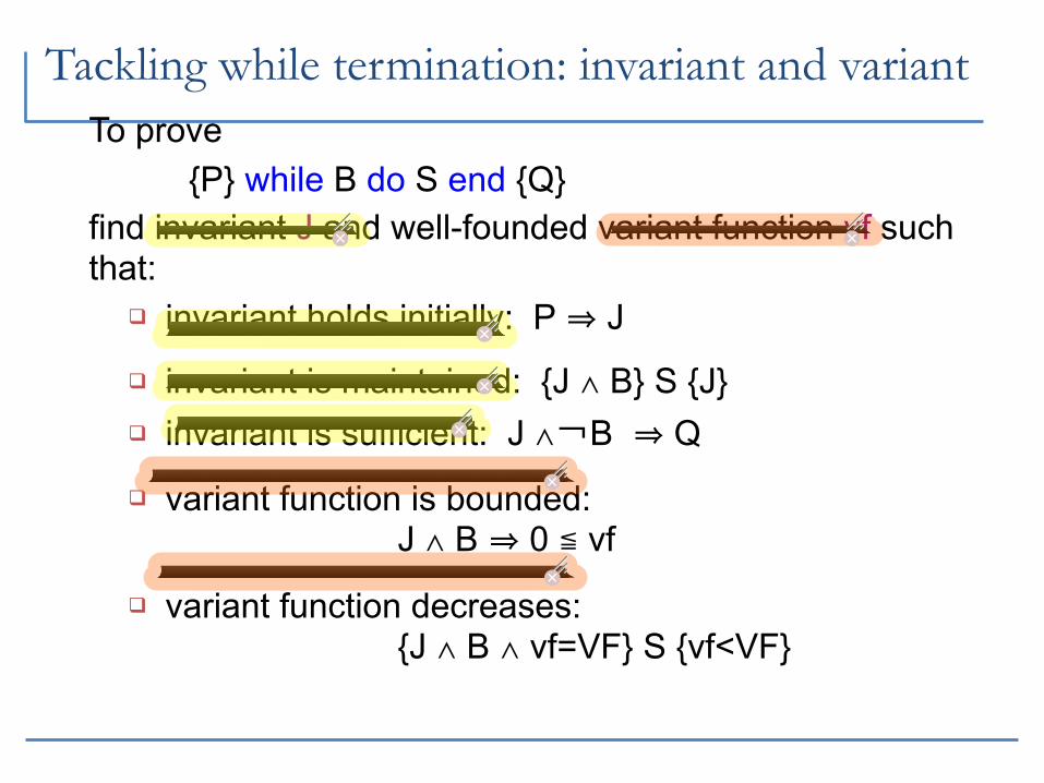
To prove {P} while B do S end {Q}find invariant J and well-founded variant function vf such that:
invariant holds initially: P ⇒ J
invariant is maintained: {J ∧ B} S {J} invariant is sufficient: J ∧¬B ⇒ Q
variant function is bounded: J ∧ B ⇒ 0 ≦ vf
variant function decreases: {J ∧ B ∧ vf=VF} S {vf<VF}
Tackling while termination: invariant and variant
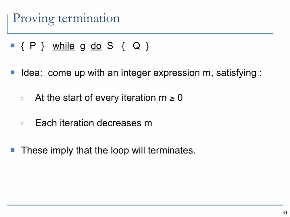
Proving termination
{ P } while g do S { Q }
Idea: come up with an integer expression m, satisfying :
q At the start of every iteration m ≥ 0
q Each iteration decreases m
These imply that the loop will terminates.
44
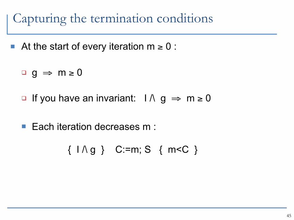
Capturing the termination conditions
At the start of every iteration m ≥ 0 :
g ⇒ m ≥ 0
If you have an invariant: I /\ g ⇒ m ≥ 0
Each iteration decreases m :
{ I /\ g } C:=m; S { m<C }
45
To Summarize
46
To Summarize
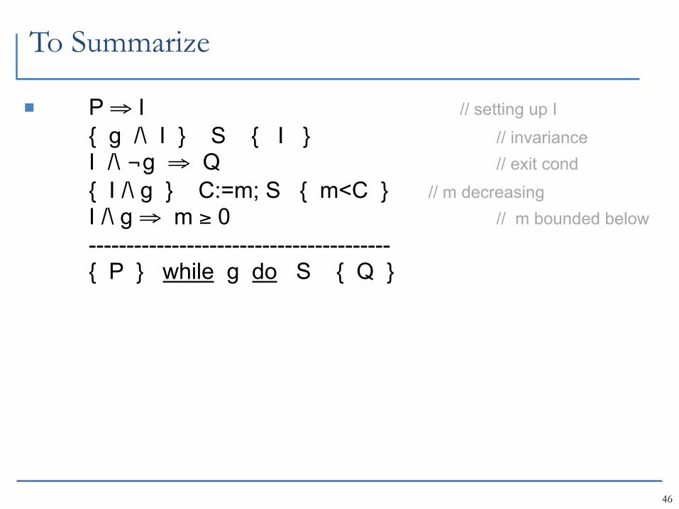
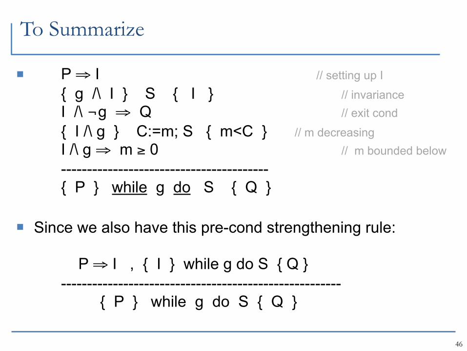
P ⇒ I // setting up I
{ g /\ I } S { I } // invariance I /\ ¬g ⇒ Q // exit cond
{ I /\ g } C:=m; S { m<C } // m decreasing I /\ g ⇒ m ≥ 0 // m bounded below ---------------------------------------- { P } while g do S { Q }
46
To Summarize
P ⇒ I // setting up I
{ g /\ I } S { I } // invariance I /\ ¬g ⇒ Q // exit cond
{ I /\ g } C:=m; S { m<C } // m decreasing I /\ g ⇒ m ≥ 0 // m bounded below ---------------------------------------- { P } while g do S { Q }
Since we also have this pre-cond strengthening rule:
P ⇒ I , { I } while g do S { Q } ------------------------------------------------------ { P } while g do S { Q }
46

A Bit History and Other Things
48
49
History
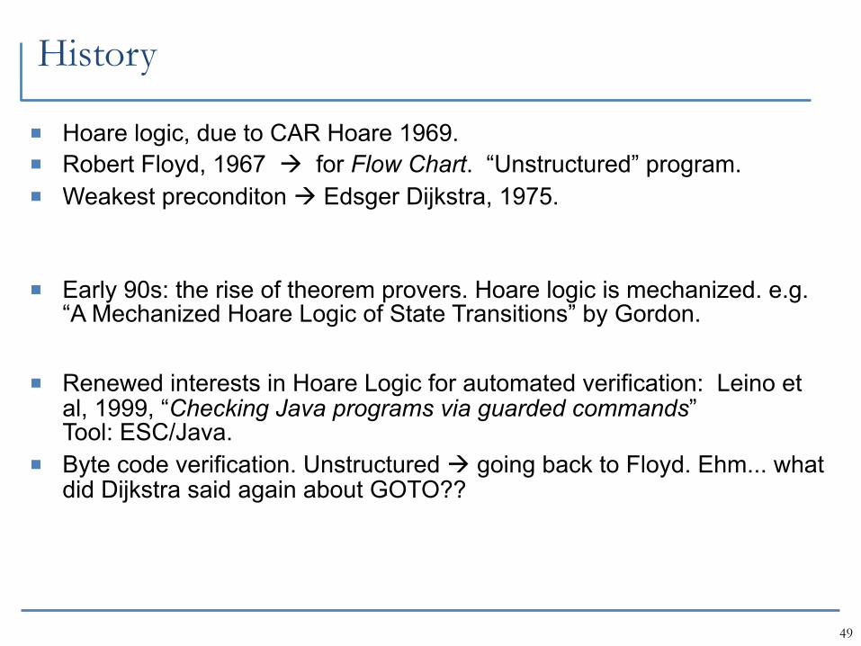
Hoare logic, due to CAR Hoare 1969. Robert Floyd, 1967 for Flow Chart. “Unstructured” program. Weakest preconditon Edsger Dijkstra, 1975.
Early 90s: the rise of theorem provers. Hoare logic is mechanized. e.g. “A Mechanized Hoare Logic of State Transitions” by Gordon.
Renewed interests in Hoare Logic for automated verification: Leino et al, 1999, “Checking Java programs via guarded commands”Tool: ESC/Java.
Byte code verification. Unstructured going back to Floyd. Ehm... what did Dijkstra said again about GOTO??
50
History
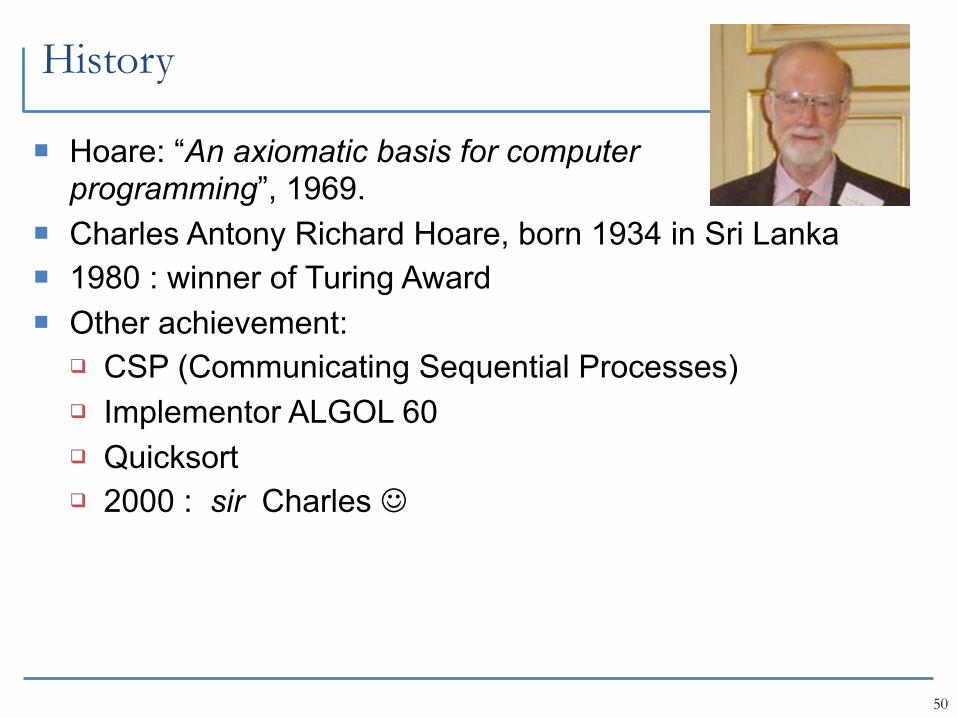
Hoare: “An axiomatic basis for computer programming”, 1969.
Charles Antony Richard Hoare, born 1934 in Sri Lanka 1980 : winner of Turing Award Other achievement:
CSP (Communicating Sequential Processes) Implementor ALGOL 60 Quicksort 2000 : sir Charles
51
History
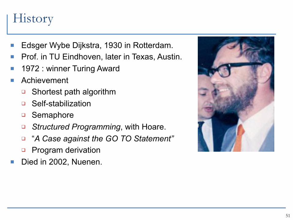
Edsger Wybe Dijkstra, 1930 in Rotterdam. Prof. in TU Eindhoven, later in Texas, Austin. 1972 : winner Turing Award Achievement
Shortest path algorithm Self-stabilization Semaphore Structured Programming, with Hoare. “A Case against the GO TO Statement” Program derivation
Died in 2002, Nuenen.
History of Programming Languages Giuseppe De
Giacomo52
ALGOL-60 ALGOL-60: “ALGOrithmic Language”
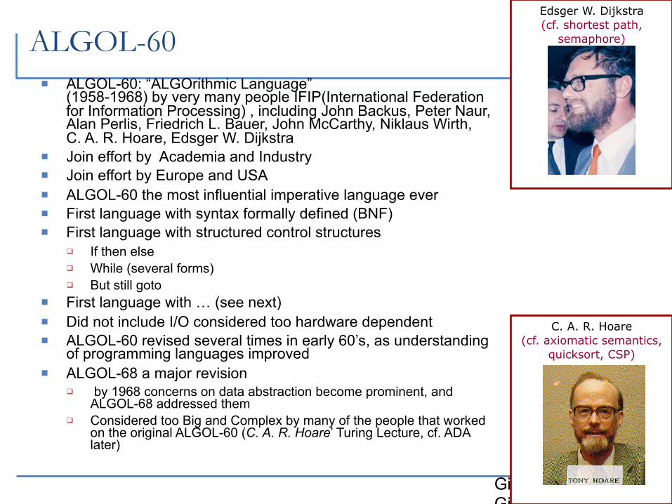
(1958-1968) by very many people IFIP(International Federation for Information Processing) , including John Backus, Peter Naur, Alan Perlis, Friedrich L. Bauer, John McCarthy, Niklaus Wirth, C. A. R. Hoare, Edsger W. Dijkstra
Join effort by Academia and Industry Join effort by Europe and USA ALGOL-60 the most influential imperative language ever First language with syntax formally defined (BNF) First language with structured control structures
If then else While (several forms) But still goto
First language with … (see next) Did not include I/O considered too hardware dependent ALGOL-60 revised several times in early 60’s, as understanding
of programming languages improved ALGOL-68 a major revision
by 1968 concerns on data abstraction become prominent, and ALGOL-68 addressed them
Considered too Big and Complex by many of the people that worked on the original ALGOL-60 (C. A. R. Hoare’ Turing Lecture, cf. ADA later)
Edsger W. Dijkstra (cf. shortest path,
semaphore)
C. A. R. Hoare (cf. axiomatic semantics,
quicksort, CSP)
History of Programming Languages Giuseppe De
Giacomo53
ALGOL-60 First language with syntax formally defined (BNF)
(after such a success with syntax, there was a great hope to being able to formally define semantics in an similarly easy and accessible way: this goal failed so far)
First language with structured control structures If then else While (several forms) But still goto
First language with procedure activations based on the STACK (cf. recursion)
First language with well defended parameters passing mechanisms Call by value Call by name (sort of call by reference) Call by value result (later versions) Call by reference (later versions)
First language with explicit typing of variables First language with blocks (static scope) Data structure primitives: integers, reals, booleans, arrays of any
dimension; (no records at first), Later version had also references and records (originally
introduced in COBOL), and user defined types
Edsger W. Dijkstra (cf. shortest path,
semaphore)
C. A. R. Hoare (cf. axiomatic semantics,
quicksort, CSP)
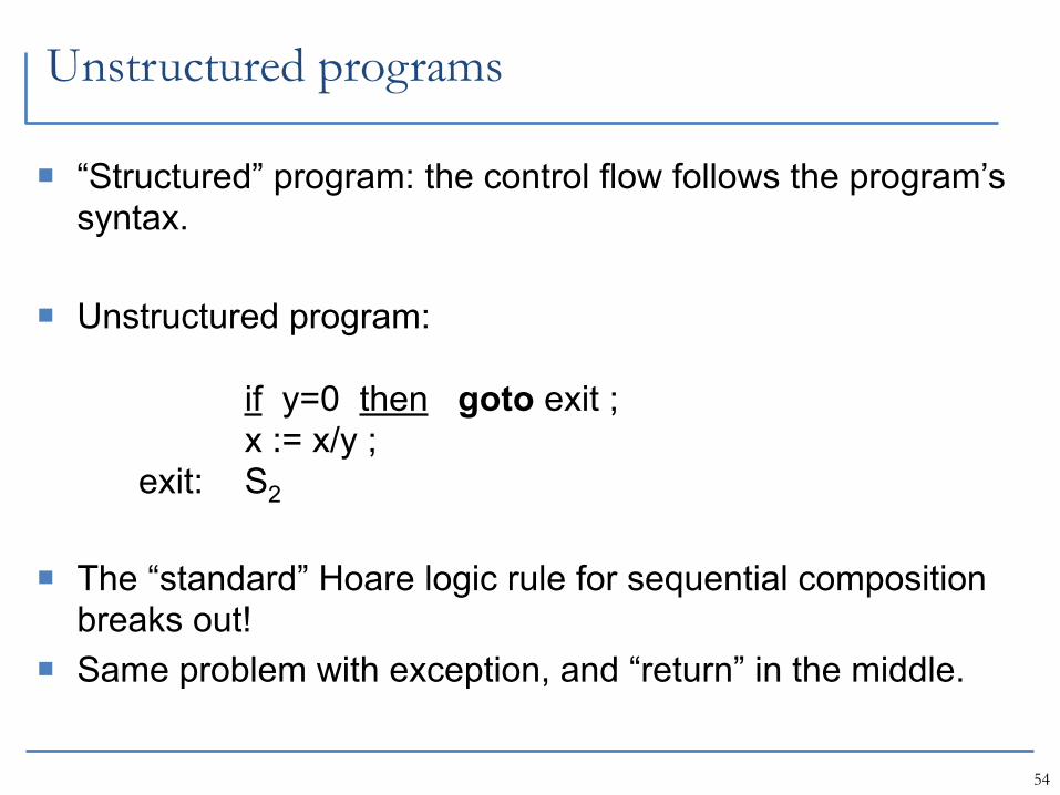
Unstructured programs
54
Unstructured programs
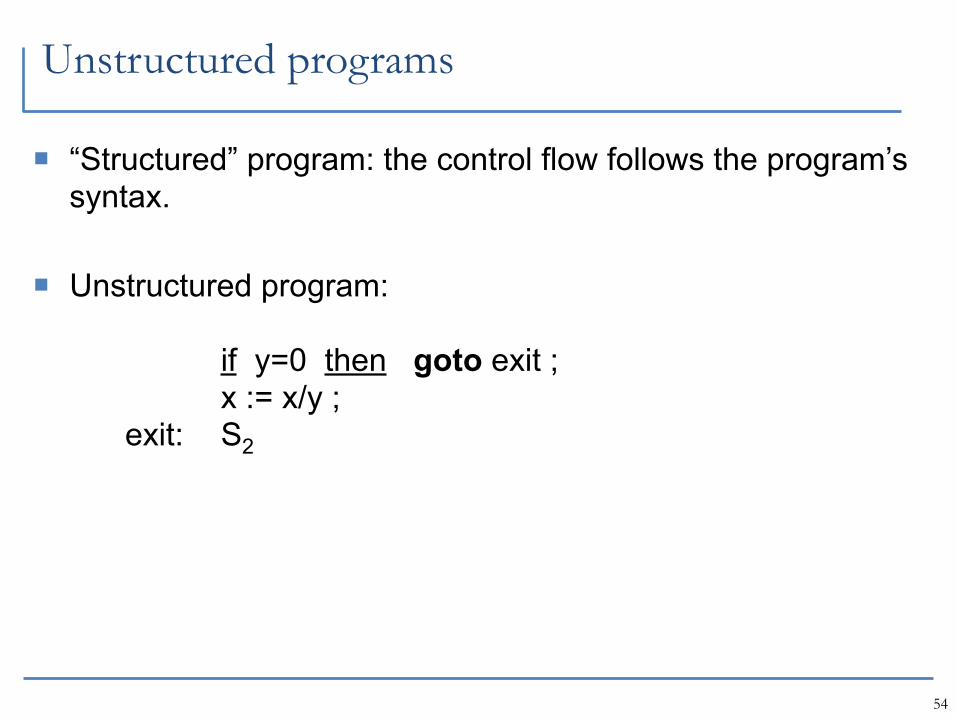
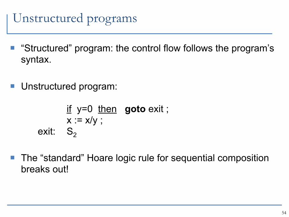
“Structured” program: the control flow follows the program’s syntax.
54
Unstructured programs
“Structured” program: the control flow follows the program’s syntax.
Unstructured program:
if y=0 then goto exit ; x := x/y ; exit: S2
54
Unstructured programs
“Structured” program: the control flow follows the program’s syntax.
Unstructured program:
if y=0 then goto exit ; x := x/y ; exit: S2
The “standard” Hoare logic rule for sequential composition
breaks out!
54
Unstructured programs
“Structured” program: the control flow follows the program’s syntax.
Unstructured program:
if y=0 then goto exit ; x := x/y ; exit: S2
The “standard” Hoare logic rule for sequential composition
breaks out! Same problem with exception, and “return” in the middle.
54
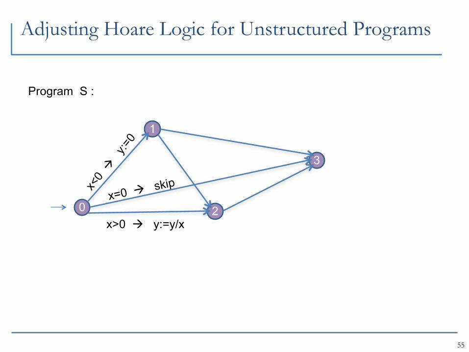
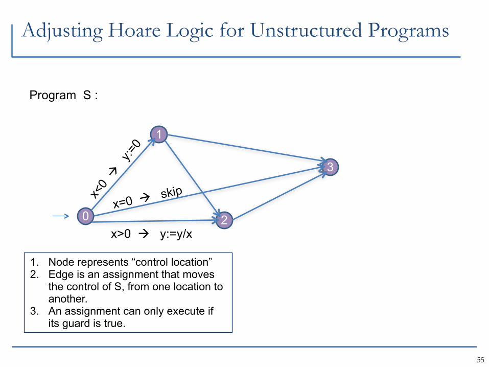
Adjusting Hoare Logic for Unstructured Programs
55
0
1
2
3
x<0
y:=0
x>0 y:=y/x
x=0 skip
Program S :
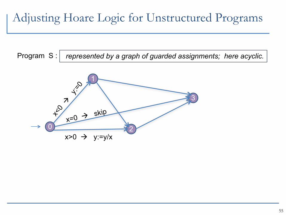
Adjusting Hoare Logic for Unstructured Programs
55
0
1
2
3
x<0
y:=0
x>0 y:=y/x
x=0 skip
Program S : represented by a graph of guarded assignments; here acyclic.
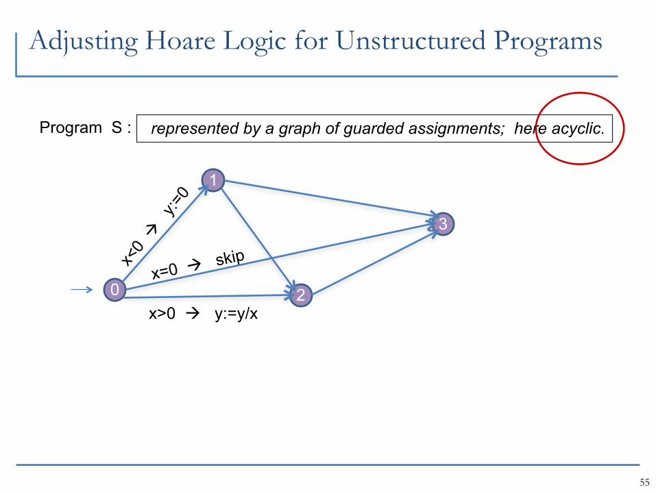
Adjusting Hoare Logic for Unstructured Programs
55
0
1
2
3
x<0
y:=0
x>0 y:=y/x
x=0 skip
Program S : represented by a graph of guarded assignments; here acyclic.
Adjusting Hoare Logic for Unstructured Programs
55
0
1
2
3
x<0
y:=0
x>0 y:=y/x
x=0 skip
Program S :
1. Node represents “control location”2. Edge is an assignment that moves
the control of S, from one location to another.
3. An assignment can only execute if its guard is true.
Adjusting Hoare Logic for Unstructured Programs
56
0
1
2
3
x<0
y:=0
x>0 y:=y/x
x=0 skip
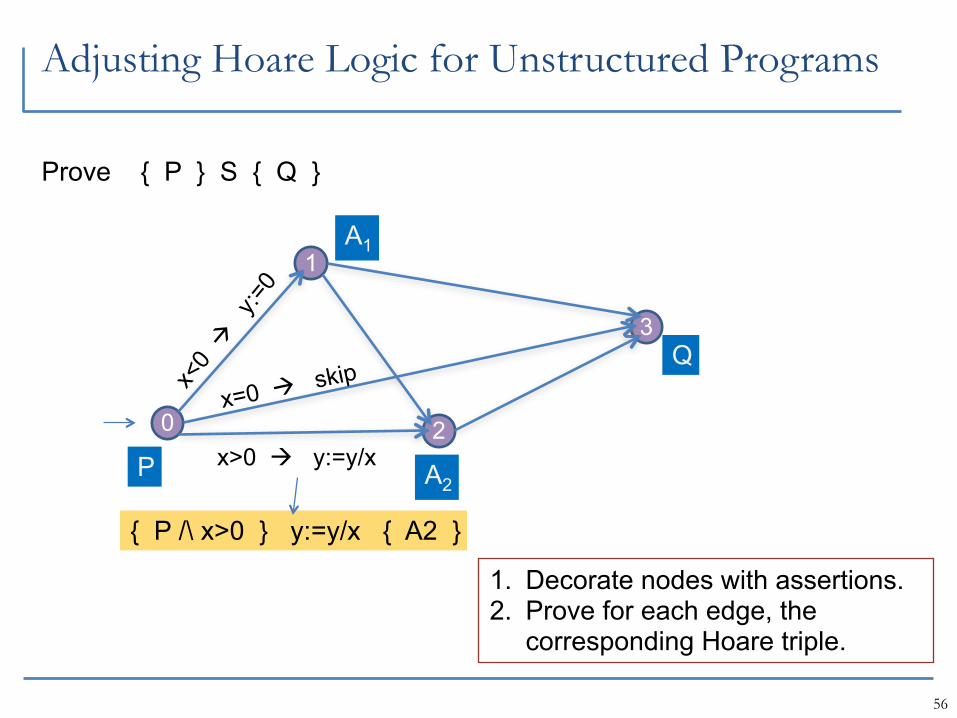
Prove { P } S { Q }
Adjusting Hoare Logic for Unstructured Programs
56
0
1
2
3
x<0
y:=0
x>0 y:=y/x
x=0 skip
Prove { P } S { Q }
1. Decorate nodes with assertions.2. Prove for each edge, the
corresponding Hoare triple.
Adjusting Hoare Logic for Unstructured Programs
56
0
1
2
3
x<0
y:=0
x>0 y:=y/x
x=0 skip
Prove { P } S { Q }
1. Decorate nodes with assertions.2. Prove for each edge, the
corresponding Hoare triple.
P
Q
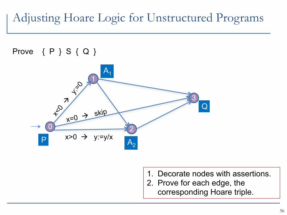
Adjusting Hoare Logic for Unstructured Programs
56
0
1
2
3
x<0
y:=0
x>0 y:=y/x
x=0 skip
Prove { P } S { Q }
1. Decorate nodes with assertions.2. Prove for each edge, the
corresponding Hoare triple.
P
Q
A1
A2
Adjusting Hoare Logic for Unstructured Programs
56
0
1
2
3
x<0
y:=0
x>0 y:=y/x
x=0 skip
Prove { P } S { Q }
1. Decorate nodes with assertions.2. Prove for each edge, the
corresponding Hoare triple.
P
Q
A1
A2
{ P /\ x>0 } y:=y/x { A2 }
Handling exception and return-in-the-middle
Map the program to a graph of control structure, then simply apply the logic for unstructured program.
Example:
try { if g then throw ; S }
handle T ;
Example:
if g then return ; S ; return ;
57
T
S
g
¬g
S
g
¬g
Beyond pre/post conditions
Class invariant
When specifying the order of certain actions within a program is important: E.g. CSP
When sequences of observable states through out the execution have to satisfy certain property: E.g. Temporal logic
When the environment cannot be fully trusted: E.g. Logic of belief
58


![Developing a Web-Based Hoare Logic Proof Assistant · 2016. 4. 28. · Hoare logic [1] (also known as axiomatic semantics) is a family of formal sys-tems for reasoning about properties](https://img.pdfslide.us/doc/110x75/5fc4dccbf3bb2e5e9271ebbb/developing-a-web-based-hoare-logic-proof-assistant-2016-4-28-hoare-logic-1.jpg)