Embed Size (px)
DESCRIPTION
dtr
Citation preview

Well Test Analysis
1
PCB 3013Well Test Analysis
Instructor:Prof. Dr. Mustafa Onur
Schlumberger Professorial ChairSchlumberger Professorial Chair
September 2013 Semester – PE Department UTP09 September -13 December 2013
Assistants (GAs) for the Course:• Mohamed Ali Hamid• Azeb Demisi Habte
General• Instructor: Mustafa Onur• Office: 16.03.04• Office Hours:
– Wednesday 9:00-11:00 am.
2
– Friday 9:00-11:00 am
• Phone: (05) 368-7099• E-mail: [email protected]• Course notes, handouts, homework, and test
solutions will be available at e-learning system.• HWs will be graded by the GAs.
AssessmentAssessment• Final Exam 40%• Course work 60%
Course work:» Test 1 (23 October 2013, 4-6 pm) 20%» Test 2 (11 December 2013, 4-6 pm) 20%» Assignment(5-10) 20%
Total 60%
General Remarks
• On each exam, you will be responsible forall material covered to that point in thecourse.
• The date of the final is fixed. It is possible,but unlikely that the times of the otherexams will be changed.

Well Test Analysis
2
General Remarks– There will be no makeup of tests. If you
miss a test, you will receive a zero on theexam. unless (i) you notify me prior to theexam that you will miss it and (ii) have amedical excuse that is supported by app yletter from a medical doctor.
– You cannot pass this course withouttaking the final exam.
– The University policy on attendance andcheating will be enforced.
Weekly Timetable
Course outlineWks Date Chapters Remarks
1-3 9 Sept. – 23 Sept. 1. Introduction & fundamental s (basic methodology , data and equation)
3-5 23 Sept – 07 Oct. 2. Drawdown , Buildup , Interference Tests
5-7 07 Oct. – 24 Oct. 3. Semilog and Type Curve Matching TEST 1
Mid -Semester Break (24-27 October)
7-9 28 Oct. -11 Nov. Superposition in Space (Linear Discountunities)
9-11 11 Nov. - 25 Nov.Superposition in Time (Buildup and Multi rate Testing)
11-13 25 Nov. – 09 Dec. Gas Well Testing
13-14 09 Dec. – 13 Dec.Other well tests and new advances (wire Line Formation Testing and complex well and reservoir systems
TEST 2
Study Week (14-18 December) and Exam Week (19-29 December)
References• Horne, R.N. (1995), Modern Well Test Analysis, Petroway
• L.P. Dake (1981), Fundamentals of Reservoir Engineering (Chapters 5-8).
• R. C. Eourlougher (1977), Advances in Well Test Analysis, SPE Monograph No. 5.Monograph No. 5.
• J. Lee, (1982), Well Testing, SPE, New York.• D. Bourdet (2002), Well Test Analysis: The Use of Advanced
Interpretation Models, Elsevier Science. • Kuchuk, F., Onur, M, Hollaender, F. (2010). Pressure Transient
Formation and Well Testing: Convolution, Deconvolution and Nonlinear Estimation, Elsevier, 2010.
• Medhat M. Kamal (Editor) (2009). SPE Monograph, Volume 23, Transient Well Testing,

Well Test Analysis
3
Course Learning Outcomes
• Fundamental knowledge on well testing and its methodology.
• Knowledge of basic theory and physics
At the end of this course, the students will be equippedwith:
(including mathematical equations) describing pressure transient fluid flow in porous media and its applications.
• Basic knowledge on conventional and modern pressure transient analysis methods.
• Information needed on well test design to improve the students’ quantitative capabilities in solving reservoir engineering problems.
Introduction to Pressure Transient Test (PTT)
Instructional Objectives1. List 4 objectives of pressure transient
testing.
2. Understand the basic methodology of PTT interpretation and analysis
3. Define testing variables.
4. Be familiar with various fluid and rock properties of reservoir systems.
What Is A Pressure Transient Test?
• A pressure transient test is a field experiment, that is like any experiment, partially controlled.
• It cannot be repeated under the same conditions, but can be rerun using the results from earlier test (experiments)test (experiments).
• There are many ways to interpret pressure transient test data; There are many models with a set of parameters that may match the observed data, but there is only one correct and more than a few probable answers.
(Source: Kuchuk, Onur, Hollaender, 2010; Pressure Transient Formation and Well Testing)
What Is A PTT…?• A tool for well and reservoir evaluation and
characterization
– Investigates a much larger volume of the reservoir than cores or logsese o t a co es o ogs
– Provides estimate of porosity, permeability under in-situ conditions
– Provides estimates of near-wellbore condition– Provides estimates of distances to boundaries

Well Test Analysis
4
Primary Objective of PTT• is to obtain the productivity of a well and
properties of the formation from downhole and/or surface pressure and flow-rate measurements.
• The formation and reservoir information obtained from pressure transient measurements are essential (Why)– They reflect the in-situ dynamic
properties of the reservoir under realistic production/injection conditions.
How Is A PTT Conducted?
q
qq = 0
t
t
p
0
Some Definitions
The rate change at the surface or subsurface creates pressure diffusion (transient) in porous, but permeable formations. The pressure diffuses away from the wellboreThe pressure diffuses away from the wellbore deep into formation and contains (brings) information about the properties and characteristics of the reservoir.This process is traditionally called pressure transient well testing.
Pressure Diffusion Process-Limited Entry Well
Probe
Dual packer interval
t = 0.05 hour t = 0. 5 hour

Well Test Analysis
5
Some Definitions (Cont’d)
• Drill Stem Testing (DST) is also part of pressure transient testing.
• Pressure transient tests are also d t d ith Wi li F ticonducted with Wireline Formation
Testers (WFT). Such tests are called wireline formation pressure transient tests.
• DSTs and WFTs are usually run in exploration and appraisal wells.
Well Testing vs. Formation Testing
• A well test may last from several days toseveral weeks and even months, and henceprovide information on reservoir over a largescale. Large volumes are produced/injected.
Both are subsets of PTT.
• On the other hand, WFTs refer to small scaletests with low flow rate and short duration (e.g.,from a few minutes to a few hours).
Both obey the same law of physics and cantheoretically be interpreted in the same way, butnote their scales are different.
Wireline Formation Testing Interval Pressure Transient Testing (IPTT)(MDT†)
Vertical 2 Vertical 2
Vertical 1
† Trade mark of Schlumberger.
SinkHorizontal
Vertical 110.3
2.3 ftDual-Packer 6.4
14.4Vertical 1
3.2
Allows determination of vertical continuityand horizontal and vertical permeability

Well Test Analysis
6
IPTT
Vertical 2
Vertical 1
er 1
2
Probe 2
Probe 1
Dual-Packer zo1
zo2Vertical 1
hw
er 2
er 3
zo1
zo2
IPTT - Wireline Formation Testing • It provides dynamic in-situ information about discrete
permeability distribution (kh and kv) along thewellbore in the medium scale (1 foot to 100 ft).
• Identify and test possible barriers andIdentify and test possible barriers andfaults/fractures in the vertical directions (or in generalalong the wellbore axis).
• Provides information on the scale of a simulationgrid.
• Cost effective and no production to surface.
“Slug” and DST Tests DST Response

Well Test Analysis
7
Primary Objective of PTT• When pressure transient test data are
incorporated into with geoscience data such as geophysical, geological, core, log, etc., it considerably improves reservoir characterization.
• Particularly, when the long-term production data are not available for undeveloped reservoirs, it is necessary to complement the volumetric estimate of oil or gas in-place with long duration well tests to estimate well productivity and reservoir size before the optimization of the field development.
A Note on Scale
μm
H2O molecules
Earth to sun
mm cm m
Well Tests
core sample
Visible light
Well Logs
WFTs
10-10 10-7 10-6 10-5 10-4 10-3 1011107
Earth diameter
10-2 10-1 100 101 102 103
deepest sediment
wellbore diameter
pore sizes
vugs
Microscopic scale(Navier stokes and Poiseuille Equation)
Macroscopic scale(Darcy’s equation and continuum approach)
A Note on Scale… Reservoir Characterization
• It is a process of building (or coming up with) a reservoir simulation model including spatial variability of rock/fluid properties and boundaries that inegrates and satisfies allboundaries that inegrates and satisfies all sources of data available (static and dynamic data) to reduce gelogical uncertainties in performance predictions.
• The purpose is to define a well/reservoir model that honors both static and dynamic knowledge about the well/reservoir system.

Well Test Analysis
8
Tools for Reservoir Characterization• Well/Formation/Reservoir Evaluation:
– Core Analysis/Petrophysics– Wireline Well Logs– Production Logging (Flowmeter)– Pressure Transient Formation and Well– Pressure Transient Formation and Well
Testing– Measurement While Drilling (MWD)– Borehole Geophysics
• Siesmics (2D, 3D, or even 4D)• Geostatistics (stochastic modeling)• Upscaling and Numerical Reservoir Simulation
Reservoir Characterization
Scale
Source: Tiab
Numerical Reservoir Simulation
F i PorositFacies Porosity
PermSw

Well Test Analysis
9
Numerical Reservoir SimulationReservoir Management Process
GeologicalData/Model
Geophysical Data/Model
Geochemical Data/Model
PetrophysicalData/Model
GeomechnanicalData/Model
FluidData/Model
Drilling
ProductionLogging Model
Tracer
Well TestModel
Integration
static data dynamic data
TracerModel
ProductionData
g
Well/Reservoir Model
upscaling
Numerical Simulation Model
Calibrated Simulation Model
Performance Prediction
history matching
Well Performance
Well Performance
Source: Gringarten (2007)
Well Performance/Production Optimization
Source: Gringarten (2007)

Well Test Analysis
10
Role of PTT in Reservoir Characterization
• PTT belongs to the dynamic part of the characterization process.
• The contribution of pressure transient testing is the well test interpretation model.
• This model is part of well and reservoir performance predictions.
How Is A PT Test Conducted?qq = 0
t
q
t
t
p
0
PTT Applications
• Exploration
• Reservoir engineeringg g
• Production engineering
PTT Objectives
• Define reservoir limits
• Estimate average drainage area pressure
• Characterize reservoir
• Diagnose productivity problems
• Evaluate stimulation treatment effectiveness

Well Test Analysis
11
Types of PTTq
Single-Well Multi-Well
Productivity Testing• The primary purpose of well testing is the
determination of the Productivity Index and the average reservoir pressure
– Used for designing tubulars and artificial lift systems.
Productivity Index• Productivity Index is a measure of the well's
ability to produce fluids under an imposed reservoir pressure drop.
J Productivity Index, STB/d/psi
Average pressure in drainage area, psia
Bottomhole flowing pressure, psia
Production rate, STB/day
( )wf
q tJ
p p=
−
( )tp( )tpwf
( )tq
Productivity Index• Function of many parameters
– Transmissibility, kh/μ– Storativity, φcth
“Ski ” d– “Skin” damage, s– Drainage area of the well, A– Reservoir and well geometry
Can we determine individual values of theseparameters?
Well Test Analysis
12
Productivity Tests Productivity Tests[ ] scwfwfsc q
JppppJq 1−=⇒−=
Is Well A or B more productive?
Why is Well C exhibiting a curvedy gbehavior instead of straight-line?
Productivity Tests[ ] scwfwfsc q
JppppJq 1−=⇒−=
Is Well A or B more productive?
Why is Well C exhibiting a curvedy gbehavior instead of straight-line?
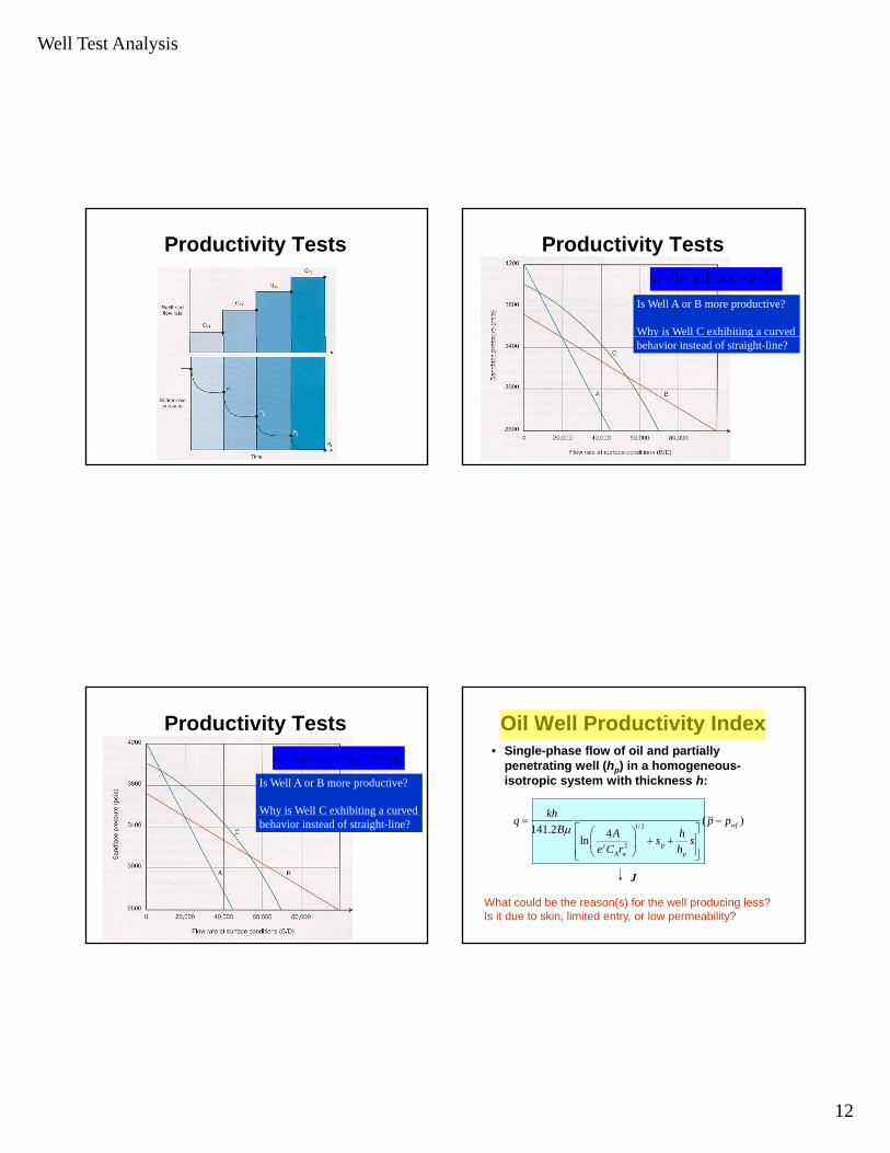
Oil Well Productivity Index• Single-phase flow of oil and partially
penetrating well (hp) in a homogeneous-isotropic system with thickness h:
kh1/ 2
2
( )141.2 4ln
wf
pA w p
khq p pB A hs s
e C r hγ
μ= −
⎡ ⎤⎛ ⎞⎢ ⎥+ +⎜ ⎟⎢ ⎥⎝ ⎠⎣ ⎦
J
What could be the reason(s) for the well producing less?Is it due to skin, limited entry, or low permeability?
Well Test Analysis
13
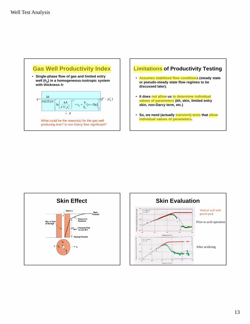
Gas Well Productivity Index• Single-phase flow of gas and limited entry
well (hp) in a homogeneous-isotropic system with thickness h:
What could be the reason(s) for the gas well producing less? Is non-Darcy flow significant?
J
( )
2 21/ 2
2
( )1422 4ln
wf
pA w w
khq p pT z A hs s Dq
e C r hγ
μ= −
⎡ ⎤⎛ ⎞⎢ ⎥+ + +⎜ ⎟⎢ ⎥⎝ ⎠⎣ ⎦
Limitations of Productivity Testing• Assumes stabilized flow conditions (steady state
or pseudo-steady state flow regimes to be discussed later).
• It does not allow us to determine individual values of parameters (kh, skin, limited entry skin, non-Darcy term, etc.)
• So, we need (actually transient) tests that allow individual values of parameters.
Skin Effect Skin EvaluationVertical well with gravel pack
Prior to acid operation
After acidizing

Well Test Analysis
14
Skin EvaluationVertical well with gravel pack
1000 4300 6300
Drawdown Testing
Rat
eq,
STB
/D
q=0
q > 0
Bot
tom
-hol
e pr
essu
re, p
wf,
psi
q
time
time
t1
t1
Buildup Testing
Rat
eq,
STB
/D
q =0
q > 0
Bot
tom
-hol
e pr
essu
re p
wf,
psi
q
time
time
t1
t1
drawdown
buildup
Injection/Falloff Testing

Well Test Analysis
15
Variable Rate Testing “Slug” and DST Tests
DST Response Multi-Well Testing
Well Test Analysis
16
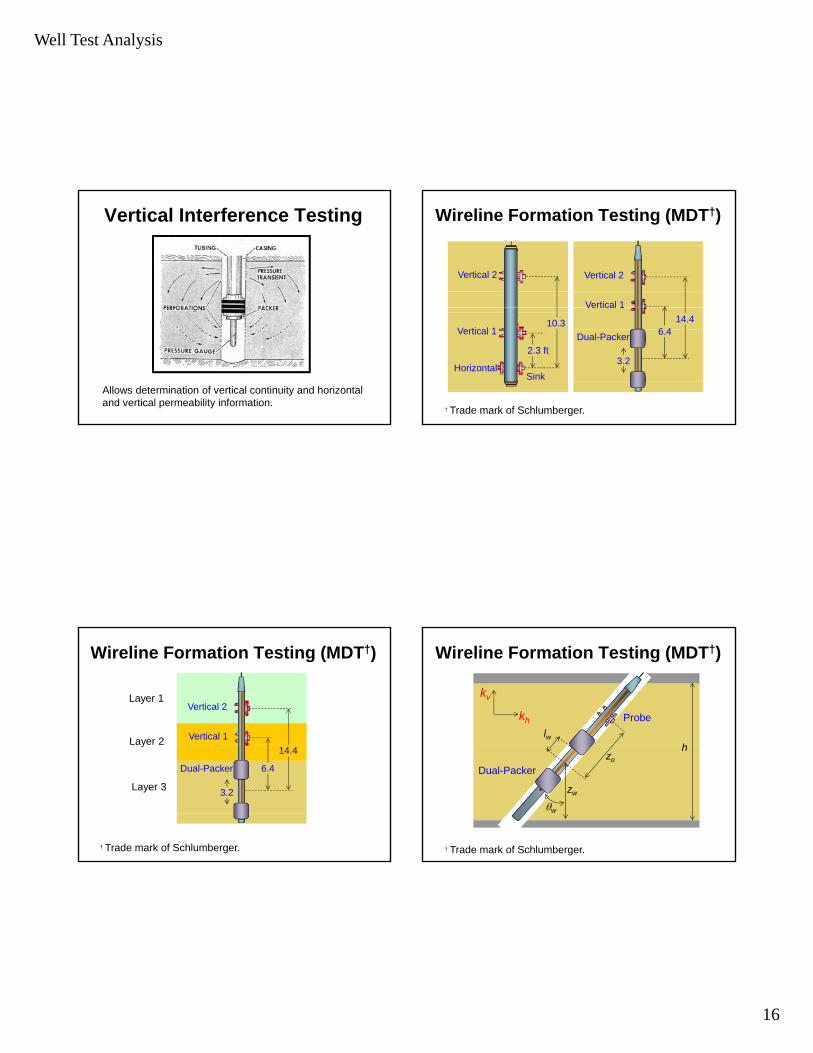
Vertical Interference Testing
Allows determination of vertical continuity and horizontaland vertical permeability information.
Wireline Formation Testing (MDT†)
Vertical 2 Vertical 2
Vertical 1
† Trade mark of Schlumberger.
SinkHorizontal
Vertical 110.3
2.3 ftDual-Packer 6.4
14.4Vertical 1
3.2
Wireline Formation Testing (MDT†)
Vertical 2
Vertical 1
Layer 1
Layer 2
† Trade mark of Schlumberger.
Dual-Packer 6.4
14.4
3.2
aye
Layer 3
Wireline Formation Testing (MDT†)
h
Probelw
kh
kv
† Trade mark of Schlumberger.
Dual-Packer
h
zw
zo
θw

Well Test Analysis
17
Summary on PTT Types…• In summary, a basic pressure transient
test consists of a production/injection rate change, during which the wellbore pressure is measured in general the d h l ddownhole, and
• Production is monitored (measured directly or in directly) either at the wellbore or surface, a subsequent buildup/falloff period during which the wellbore pressure is usually measured downhole.
Basic Steps of PTT Interpretation
• It involves three basic steps:
– Step 1: Model Identification– Step 2: Estimation of model parameters – Step 3: Validation of results
Interpretation Methodology of PTTs
• During a well test, a transient response is created by a temporary and controlled change in production rate.
• Then, the response (pressure, temperature and/or flow rate at bottom hole) of the well/reservoir system to changing production (or injection) is monitored.
• The response is, to a greater or lesser degree, characteristic of the properties of the well/reservoir sytsem and thus it is possible in many cases to infer well/reservoir parameters from the observed response.
Interpretation Methodology… • A Constant-Rate Drawdown-Buildup Sequence:
Rat
e, q
q > 0
RB
otto
m-h
ole
pres
sure
, pw
f, ps
i
q = 0
time
time
t1
t1
drawdown
buildup

Well Test Analysis
18
Interpretation Methodology…• Is to identify the “appropriate” interpretation model(s)
and obtain “reasonable” estimates of the formation (or reservoir) parameters of interest from indirect measurements of pressure and rate data.
• These estimates are defined in terms of a• These estimates are defined in terms of a mathematical well/reservoir model, derived based on simplified assumptions, yet from physical principles (conservation laws) governing the behavior of the system under observation.
• All monitored pressure transients in porous media are governed by some form of the diffusivity equationwith appropriate initial and boundary conditions.
Interpretation Methodology…• Pressure transient interpretation sequence is
applications of inverse/forward(direct) problems:
Real system ( S )I (rate-time)
O (observed pressure vs time)
Real system ( S )
Model (k, φ, s, etc)I (rate-time)
OM (model pressure vs time)
O ≈ OM
Matching
Forward and Inverse Problems• Inferring an interpretation model from an observed
response (or signal) is an application of inverseproblem.
• Once model is identified, estimating model parameter is application of both forward andparameter is application of both forward and inverse problems, depending on the estimation method used.
• Therefore, a mathematical (analytical/or numerical) model is required to estimate the model parameters from observed data. There are variety of models developed for pressure transient analysis.
STEP 1: Model Identification• Find a model SM which behaves in the same way
as the real system S given the input and output.
I S O OM should show thesame features of O
Inverse problemwith a non-uniquesolution
I SM OM
same features of O
To reduce non-uniqueness:-More test data: pressure/rate-Checking procedure on model-Consistency with geology, geophysics, petropyhsics, etc.

Well Test Analysis
19
STEP 1: Model Identification…• Tools for Model Identification
– Pressure-Derivative signal based on superposition time
– Pressure-Derivative signal based onPressure Derivative signal based on deconvolution
• To reduce non-uniqueness:– More test data: pressure/rate– Checking procedure on model– Consistency with geology, geophysics,
petropyhsics, etc.
STEP 1: Model Identification…
(Taken from Schlumberger Modern Reservoir Testing book)
STEP 1: Model Identification…
(Taken from Schlumberger Modern Reservoir Testing book)
(a) Well (near sealing fault)producing in homogeneous-isotropic reservoir
(b) Well producing in a naturally fractured reservoir system.
STEP 2: Model Parameter Estimation• Adjust the parameters of the MODEL SM so that
OM matches O “quite well.”
I S OI S O
I SM OM
O ≈ OM
Direct or Inverse problem depending on the method as well as quality and span of the test data.

Well Test Analysis
20
STEP 2: MP Estimation…• Tools for Model P. Estimation
– Straight line methods (semilog, Cartesian plots, etc.)
– Type-curve matching based on Pressure and/or Pressure-Derivative responses
– Non-linear regresion• To reduce non-uniqueness:
– Calculated parameters should be very similar independent of the method (or tool) used.
STEP 2: MP Estimation…
Δp'
, p
si
102
Pressure change
Closed reservoir model
Time (h)
Δp
and
10-1
10-4 10-3 10-2 10-1 100 101 102
100
101
Infinite actingreservoir
model
ttest = 3 h.
Reservoir boundary has no effecton the responses
STEP 3: Validation of Results• Verify the consistency of the interpretation model
by:– matching with test observed data (log-log,
Horner, simulation)– matching results from other well testsatc g esu ts o ot e e tests– matching with other knowledge (geology,
petrophysics, cores, fluids, completion)– common sense (range of plausible parameter
values).– Inspect confidence intervals, correlation
coefficients, RMS errors if non-linear regression is used.
PTT Interpretation (Outer Loop)
(Source: Kuchuk, Onur, Hollaender, 2010)

Well Test Analysis
21
PTT Interpretation (Inner Loop)
(Source: Kuchuk, Onur, Hollaender, 2010)
PTT Interpretation ModelsNear WellboreEffects
Reservoir Behavior
Boundary Effects
Wellborestorage Infinite actingHomogeneous
SkinFractures
Limited Entry
Horizontal/slanted well
Early times
No-flow
Constantpressure
Leaky
Late timesMiddle times
Heterogeneous2-PorosityLayeredComposite
Remarks on Reducing Uncertainty in PTT
• We should always resort to other independent sources of information (geoscience data, drilling, logs, cores).
We should carefully design tests by taking into• We should carefully design tests by taking into consideration of flow rate history to be applied, accuracy and resolution of pressure gauges.
• Perform sensitivity studies prior to testing by performing forward runs with the appropriate model(s) for the system under consideration.
Pressure-Derivative

Well Test Analysis
22
Pressure-Derivative (P-D)• It was introduced in 1980 by Bourdet et. al
and has become a standard tool in PTT Interpretation since then.
• It helps identifying the appropriate model for the system under consideration and flow regimes.
• It also helps reducing non-uniquess in parameter estimation when it is used together with pressure.
• It magnifies the changes in pressure data so it is useful for diagnostic purposes.
Pressure-Derivative• It is defined as the rate of pressure change with
respect to natural logarithm of time.
( ) ( ) dtdp
tdt
tppdt
tdtppd
tdpdp wfwfiwfi −=
−=
−=
Δ=′Δ
))((ln
))((ln
)(
Why is it based on logarithm of time?What is the unit of pressure-derivative?
Pressure-Derivative-Example 1
102
Δp'
, p
si
Circular no-flowreservoir
10-4 10-3 10-2 10-1 100 101 10210-1
100
101
Time (h)
Δp
andΔ
Pressure-derivative
Pressure-Derivative-Example 2
ndΔ
p' ,
psi
102
103
1.0=ω
Δp
Time (h)
Δp
an
10-1
100
101
10-4 10-3 10-2 10-1 100 101 102
Naturally fractured reservoir (Warren-Root, λ =10-7)
01.0=ω

Well Test Analysis
23
Some Remarks on P-D• Unlike pressure, pressure-derivative is not
measured and has to computed by numerical differentiation of the measure pressured data with respect to time.
• Differentiation amplifies the noise in pressure• Differentiation amplifies the noise in pressure data. This often causes pressure-derivative data to oscillate wildly and complicate model identification and parameter estimation.
• To eliminate the oscillatory behavior, we often apply smoothing methods to pressure derivative.
P-D Computation• It is computed by numerical differentiation of
the measure pressured data with respect to time.
ΔpΔpj+1
t
Δpj
Δpj-1
lntj-1 lntj lntj+1
( ) ( )( ) ( )
( )( ) ( )
( )( ) ( )
2
11 11
1 1 1 1
11
1
1
1 1
ln /ln /
ln / ln / ln / ln /
ln /
ln / ln /
jj j jj j
j j j j j j j j
j j
j j j j
j j
j
t t tt t
t t t t t t t t
t t
p
pt t
pp
t
t
t
+−
−+
+ − − + −
+−
+ − +
′Δ − Δ Δ
Δ
= +
+
Bourdet method (2nd degree polynomial through successive three points)
P-D Computation…• Differentiation amplifies the noise in pressure
data. This often causes pressure-derivative data to oscillate wildly and complicate model identification and parameter estimation.Suppose we have equally spaced pressure dataSuppose we have equally spaced pressure data, containing uncorrelated noise with zero mean and constant standard deviation σp, and are using Bourdet method to generate pressure-derivative, then we can show that std. of noise in pressure derivative is:
1
ln constant < 1j
j
tL
t −
⎛ ⎞= =⎜ ⎟⎜ ⎟
⎝ ⎠
12d pL
σ σ=
Noise in derivative data will also be correlated, though noise in pressure is not, see SPE 71579
Effect of Noise on P-D
Well Test Analysis
24
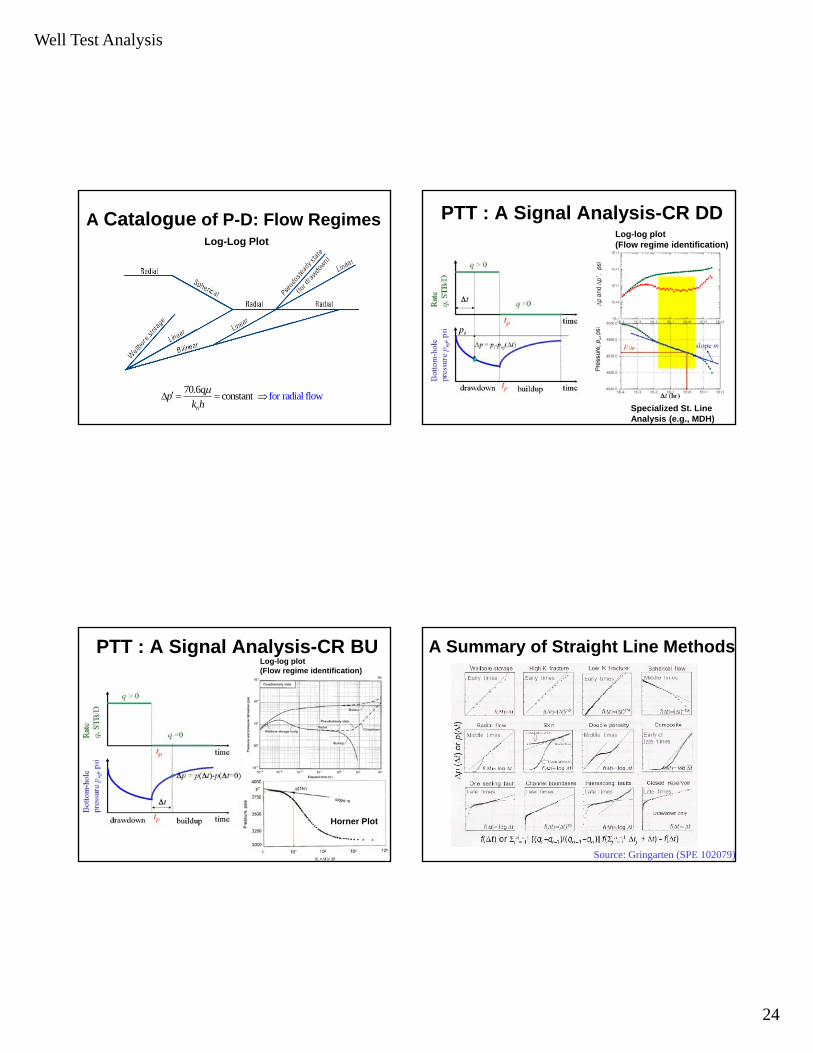
A Catalogue of P-D: Flow RegimesLog-Log Plot
70.6 constan for radial ft lowh
qpk h
μ′Δ = = ⇒
PTT : A Signal Analysis-CR DD Log-log plot(Flow regime identification)
Specialized St. LineAnalysis (e.g., MDH)
PTT : A Signal Analysis-CR BU Log-log plot(Flow regime identification)
Horner Plot
A Summary of Straight Line Methods
Source: Gringarten (SPE 102079)

Well Test Analysis
25
Interpration of PTTs
• We attempt to recognize specific flow regimes exhibited (on log-log plot) thatregimes exhibited (on log log plot) that dominate the data behavior to identify the appropriate interpretation model.
Various Flow Regimes
Various Flow Regimes…
H (IARF) High conductivity fractureHomogeneous (IARF) High conductivity fracture
2-Porosity or Multilayer Composite or Multiphase Fluid
Various Flow Regimes…
Source: Gringarten (SPE 102079)

Well Test Analysis
26
Various Flow Regimes…
Source: Gringarten (SPE 102079)
History of PTT AnalysisDate Analysis Method Emphasis Identification Verification
50s Straight lines Homogeneous reservoir
Poor None
70s Pressure Type Curves
Near wellbore effects, 2-
porosity, fractured wells
Fair (limited) Fair to good
80 P H V d V d
Modified from Gringarten (SPE 102079)
80s Pressure Derivatives
Heterogoneous reservoirs and
boundaries
Very good Very good
90s Non-linear Regression
Computerizedanalysis, variable
rate tests, multilayer reservoirs
Very good Much better
00s Deconvolution Computerized analysis, enhance
radius of investigation
Much better Same as Derivative