1

PARSEC Benchmark Suite: A Parallel Implementation on GPU using CUDA Abhishek Ray

raya@cs.ucr.edu University of California, Riverside

Abstract:

Graphics Processing Units (GPUs) are a class of specialized parallel

architectures with tremendous computational power. The

Compute Unified Device Architecture (CUDA) programming model

from NVIDIA facilitates programming of general purpose

applications on their GPUs. In this project, we targets Parsec

benchmarks to provide orders of performance speed up and

reducing overall execution time on multi-core GPU platforms.

Parsec benchmark suite presents and characterizes applications for

CPU computation which runs on multiprocessors for providing high

level of parallelism for specific applications. We extended seven of

the Parsec applications to the CUDA programming language which

extends parallelism to multi-GPU systems and GPU-cluster

environments. Our methodology calculates execution time at

different level for GPUs applications while varying the number and

configuration of GPUs and the size of the input data set and allows

us to look for overheads. Emphasis is placed on optimization the

applications by directly targeting the architecture to best exploit

the computational capabilities of NVIDIA Tesla T10 to achieve

substantial speed up.

1. Introduction:

The benefits of using Graphics Processing Units (GPUs) for general

purpose programming has been recognized for some time, With

multiple cores and large memory bandwidth, the computational

capability of GPU today is much higher than that of the CPU. Due

to its high computational capability, the GPU nowadays serves not

only for accelerating the graphics display but also for speeding up

non-graphics applications. General purpose GPU (GPGPU)

programming has become the scientific computing platform of

choice mainly due to the availability of standard C libraries using

NVIDIA’s CUDA programming interface running on NVIDIA

GPUs and a number of efforts have explored how to reap large

performance gains on CUDA-enabled GPUs.

This project is another effort to parallelize Parsec benchmark suite

on GPU using CUDA to provide orders of performance speed up

and reducing the overall execution time that cannot be achieved by

running on CPU platform. In our CUDA implementation we

compared CPU vs. GPU runtime for different size of inputs and

different size of threads and we tried to identify potential overheads

of each application running on GPU. Emphasis has also being made

to overcome those bottlenecks and optimize the CUDA code

running on GPU with some optimization techniques like Memory

Coalescing, Shared Memory, Cache-efficient texture memory

accesses, loop unrolling, Parallel Reduction and Page-locked

Memory allocation. CUDA compute capability 1.2 and 1.3 e.g.

GTX 280 used in this project offers specialized memory spaces

depending on the application: Per-block shared memory, constant,

and texture memories to reduce overheads. Each is suited to

different data-use patterns. Although we used some optimization

techniques to alleviate these issues, they remain a bottleneck for

some applications.

The benchmarks have been evaluated on an NVIDIA GeForce GTX

280 GPU with a 1.33 GHz core clock, on board memory of 4GB,

ultra-fast memory access with 102 GB/s peak bandwidth per GPU

and varying GPU power consumption of 160W.

The rest of this paper is organized as follows. Section 2 shows

glimpses of what kind of Parsec application has been transformed to

CUDA, CUDA architecture and general CUDA programming

model. Section 3 presents a general algorithm for CUDA

programming and requirements for optimization. Section 4 explains

details of the benchmark, their transformation to CUDA, results and

overheads and optimization techniques used in eliminating the

overheads. Section 5 presents results for execution time for different

size of inputs for different size of threads.

2. Parsec Benchmark Application and Compute

Unified Device Architecture Glimpse:

2.1. Parsec Benchmarks

The Princeton Application Repository for Shared-Memory

Computers (PARSEC) benchmark is a benchmark suite composed

of multithreaded programs. The suite focuses on emerging

workloads and was designed to contain a diverse selection of

applications in the field of data mining, computer vision,

visualization, computer animation, financial analysis etc that

represents of shared-memory programs for chip-multiprocessors. It

provides a selection of next generation workloads that satisfies the

following five criteria: 1. Composed of multithreaded applications.

2. Focuses on emerging workloads. 3. Diverse enough to represent

the increasingly heterogeneous ways in which multiprocessors are

used.4. Workloads employ state-of-art techniques. 5. Support

research

Workloads

Blackscholes This application is an Intel RMS benchmark. It

calculates the prices for a portfolio of European options analytically

with the Blackscholes partial differential equation (PDE).

Ferret This application is based on the Ferret toolkit which is used

for content-based similarity search. It was developed by Princeton

University. In the benchmark, we have configured the Ferret toolkit

for image similarity search.

Fluidanimate This Intel RMS application uses an extension of the

Smoothed Particle Hydrodynamics (SPH) method to simulate an

incompressible fluid for interactive animation purposes.

Raytrace The Intel RMS application uses a version of the

raytracing method that would typically be employed for real-time

animations such as computer games.

Streamcluster This RMS kernel solves the online clustering

problem. Streamcluster was included in the PARSEC benchmark

suite because of the importance of data mining algorithms and the

prevalence of problems with streaming characteristics.

Swaptions The application is an Intel RMS workload which uses

the Heath-Jarrow-Morton (HJM) framework to price a portfolio of

swaptions. Swaptions employs Monte Carlo (MC) simulation to

compute the prices.

2

X264 This application is an H.264 which describes the lossy

compression of a video stream and is also part of ISO/IEC MPEG-4.

2.2 CUDA

The Multi-core CPUs and GPUs have been used to exploit

parallelism in performing compute-intensive operations on

structured data, i.e. data stored in databases. However, recent trends

in data storage suggest that more and more data is being captured in

the form of images, audio and video files. As a result of continued

demand for programmability, modern graphics processing units

(GPUs) such as the NVIDIA are designed as programmable

processors employing a large number of processor cores.

The NVIDIA Tesla T10 has 30 multiprocessor units, each consisting

of 8 processor cores that execute in SIMD manner. The processors

(SIMD units) within a multiprocessor unit communicate through a

fast on-chip shared memory, while the different multiprocessor units

communicate through a slower off-chip DRAM, also called global

memory. Each multiprocessor unit also has a fixed number of

registers. The GPU code is launched for execution in the GPU

device by the CPU (host). The host transfers data to and from GPU's

global memory. Programming GPUs for general-purpose

applications is enabled through an easy-to-use C interface exposed

by the NVIDIA Compute Unified Device Architecture (CUDA)

model. CUDA programming is done with standard ANSI C

extended with keywords that designate data-parallel functions,

called kernels, and their associated data structures to the compute

devices. These kernels describe the work of a single thread and

typically are invoked on thousands of threads. The CUDA

programming model abstracts the processor space as a grid of thread

blocks (that are mapped to multiprocessors in the GPU device),

where each thread block is a grid of threads (that are mapped to

SIMD units within a multiprocessor). More than one thread block

can be mapped to a multiprocessor unit, and more than one thread

can be mapped to a SIMD unit in a multiprocessor. Threads within a

thread block can efficiently share data through the fast on-chip

shared memory and can synchronize their execution to coordinate

memory accesses. Each thread in a thread block is uniquely

identified by its thread block id and thread id. A grid of thread

blocks is executed on the GPU by running one or more thread

blocks on each multiprocessor. Threads in a thread block are

divided into SIMD groups called warps (the size of a warp for the

NVIDIA GeForce 8800 GTX is 32 threads) and periodic switching

between warps is done to maximize resource utilization.

The NVIDIA Tesla T10 contains 1.4 billion transistors, 240 cores

with streaming multiprocessor consists of 8 Streaming Processors

(SPs), 2 Special Function Units (SFUs) 16 KB R/W shared memory

and total of16384 registers. The Tesla is capable of 1 TFLOPs/s of

processing performance and comes with 4 GB of GDDR3 at 102

GB/s bandwidth. Fig 1 and 2 shows the block and grid. Block is a

collection of threads. There are upto 1024 threads per SM. Each

thread can communicate within the same block. Grid is a collection

of blocks. It is usually one per CUDA device and used for multiple

iterations. Threads cannot communicate across grids.

Fig 1: Thread Blocks and Grids

Fig 2: Memory Management

3. GPU Computing: CUDA Implementation

This section describes a basic algorithm of transformation of C to

CUDA which in cases similar for all Parsec application. Also, this

section defines basic optimization techniques used. The details of

these are explained in details in section 4.

Basic Algorithm for CUDA implementation

The GPU is seen as a compute device to execute a portion of an

application that has to be executed many times, can be isolated as a

function and which works independently on different data. Such a

function can be compiled to run on the device. The following steps

are followed for CUDA implementation for the already written C

code available in Parsec benchmarks suite 2.1.

3

Set the grid size const int N = 1024;

const int blocksize = 16;

Compute Kernel __global__void add_matrix( float* a, int N )

{int i = blockIdx.x * blockDim.x + threadIdx.x;}

CPU memory float *a = new float[N*N];

Allocation a[i] = 1.0f;; }

GPU Memory cudaMalloc( (void**)&ad, size );

Allocation

Copy data to cudaMemcpy( ad, a, size, cudaMemcpyHostToDevice

GPU

Execute the kernel dim3 dimBlock( blocksize, blocksize );

dim3 dimGrid( N/dimBlock.x, N/dimBlock.y );

add_matrix<<<dimGrid, dimBlock>>>( ad, N );

Copy data back cudaMemcpy(c,cd,size, cudaMemcpyDeviceToHost );

To CPU

Free memory cudaFree(ad ); cudaFree(bd ); cudaFree(cd );

float *ad, *bd, *cd;

const int size = N*N*sizeof(float);

3.2 Optimization

Optimization is one of the rather difficult parts of CUDA but

definitely an important to achieve a good performance. This section

gives a brief idea about common kind of optimization can be used or

rather should be used for achieving a good performance. This part

doesn’t give the details of optimization used for particular

application. The details are mentioned in the upcoming section 4 for

specific benchmark as we move further.

The optimization for each Parsec benchmark depends on specific

requirement, kind of data involved and the size of input. But the

principle for choosing optimization to the CUDA code depends on

following:

Optimize use of on-chip memory to reduce bandwidth usage

and redundant execution

Group threads to avoid SIMD penalties and memory port/bank

conflicts.

Threads within a thread block can communicate via

synchronization, but there is no built-in global communication

mechanism for all threads.

The optimization CUDA involves many different techniques but it

is important to find out what techniques are best suited for particular

application. The following optimization techniques present a brief

idea of optimization:

Global Memory Throughput (Memory Coalescing): Reducing

transaction sizes to half from actual size: Memory access is handled

per-wraps. So, we can carry out smallest possible number of

transactions. Reducing transaction size when is the first options. The

details are same as the paper by [4].

Launching Configuration: This is way of optimizing by launching

sufficient threads to hide latency. Use of threads depends on the

access pattern (global, shared or texture) but application can be

launched upto 512threads which is sufficient. Like using global

memory, it is always wise to use maximum of 512 threads but when

it comes to shared or particularly texture, using 512 threads will not

make a huge difference. The reason can be seen in NVIDIA

programming guide.

Device Memory: This is perhaps the most important optimization for

CUDA. Many applications are memory bound. So, it is important to

use right memory. There are five different memories available in

GPU: global, shared, local, constant and texture. Our experiment

shows that shared memory is best memory to be used as it allows

per block data reuse which in true in our case for many applications.

It caches data to reduce global memory accesses and avoid non-

coalesced access to provide serialization. If n threads access the

same bank, then n accesses can be executed serially (n threads

access the same word in one fetch). Rather than using only global

memory, we divide the work between global memory and shared

memory or texture memory. This affects the performance to much

extend. Before going into the application details, let us see the

memory hierarchy available in GPU.

Global memory is a large memory accessible by all threads. All

device kernel code and data must fit within global memory. The

global memory on the Tesla T10 is has a 128KB block size, and a

latency of 600-900 cycles.

Shared memory is local to each SM, and data in shared memory

may be shared between threads belonging to the same thread block.

If multiple blocks are scheduled to the same SM, shared memory

will be evenly partitioned between them. The size of the shared

memory is 16KB per SM on the Tesla. Each memory is 16-banked

and has 4 cycle latency.

Local memory provides the same latency benefits as shared

memory, but is local to the SPs and can only be accessed on a per-

thread basis. Local memory is typically used as a fast scratchpad.

Constant memory is a special partition of global memory meant to

hold constant values. It is read-only from the device scope and can

only be written to by the host. The constant memory is 2-level, with

distributed, hardware-managed caches in each SM. Because the

constant memory is read-only, these caches do not have any

coherence protocol. On the Tesla, each constant cache is 16KB and

has low access latency.

Texture memory is similar to constant memory, but also includes

support for special optimized texture transformation operations.

This extra support comes at the cost of higher latency than constant

memory for normal read operations.

4. Applications: Details, CUDA implementation,

Results and Optimization

3.1. CUDA Implementation: Transformation

3.1.1 Blackscholes: Converted from original tbb version. Used for

financial analysis. It computes prices of portfolio of European

Options with the Blackscholes PDE.

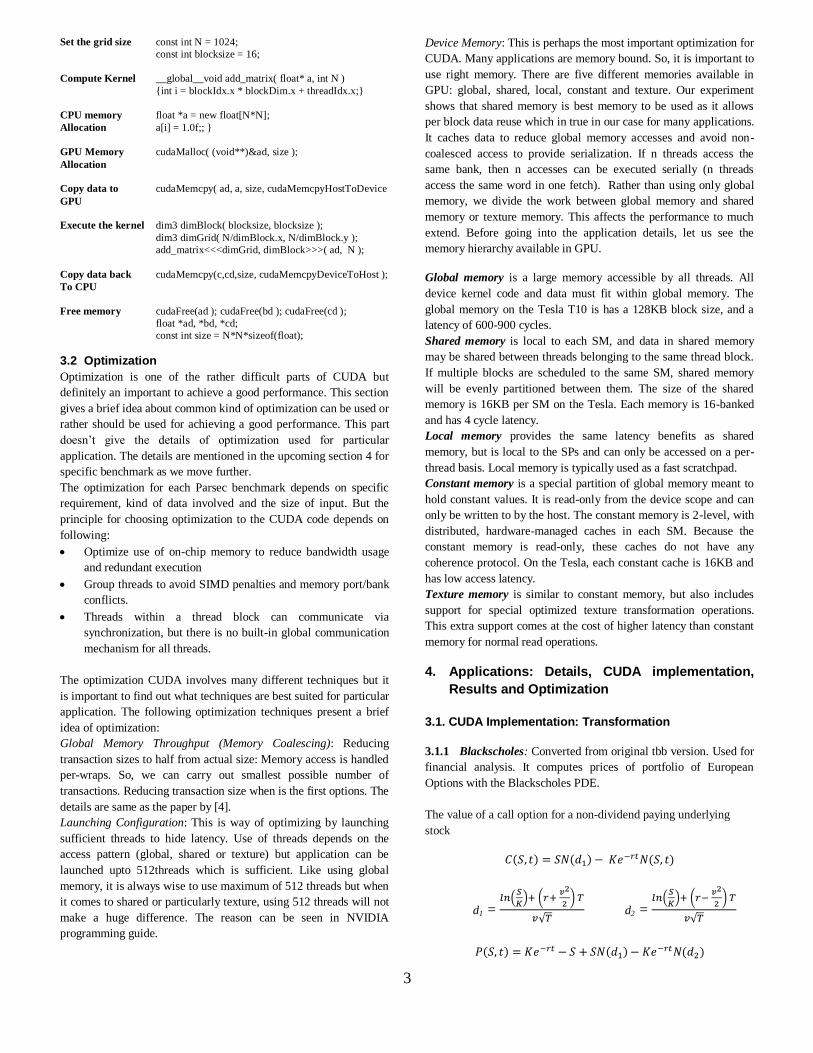
The value of a call option for a non-dividend paying underlying

stock

d1 =

d2 =

4

where N(•) is the cumulative distribution function of the standard

normal distribution, T - t is the time to maturity, S is the spot price

of the underlying asset, K is the strike price, r is the risk free rate

and T is the volatility of the underlying asset.

For CUDA implementation, blackscholes stores the portfolio with

numOptions derivatives in array OptionData. The program includes

file option-Data.txt which provides the initialization and control

reference values for 1,000 options which are stored in array data

init. The initialization data is replicated if necessary to obtain

enough derivatives for the benchmark. The CUDA program was

written in global memory. The program divides the portfolio into a

number of work units equal to the number of threads and processes

them concurrently. The transformation involves generation random

input data on host, transferring data to GPU, compute prices on

GPU, transfer prices back to host, compute prices on CPU and

check the results. Each options is calculated independently and each

thread iterates through all derivatives in its contingent and calls

function BlkSchlsEqEuroNoDiv for each of them to compute its

price. A simple implementation of the Blackscholes algorithm

would assign each thread to a specific index of input data. But there

are some hardware constraints to be taken into Block grid

dimensions on are only 16-bit (i.e. the maximum size of each

dimension is 65536 and maximum number of threads per block is

512. [See Appendix 3.2 for CUDA code.]

Initial Result:

[raya@coil release]$ blackscholes Size = 65100

options threads = 512

Throughput = 3.6903 GOptions/s Time = 1.32400 ms

Time transfer CPU to GPU = 0.4998 ms

GPU Kernel execution = 0.0425 ms

Time transfer GPU to CPU = 0.737 ms

Overheads and Optimization:

The main problem in blackscholes is the transfer time between host

to device memory and vice versa. This may be due to fact that the

PDE equations which calculates option pricing involves intense

calculation and it needs data input for that. But, blackscholes

doesn’t need all data at single time but it does access same data

again and again. It is important to reduce the transfer time by some

optimization method like global memory coalescing or page locked

memory allocation.

For CUDA optimization, blackscholes throughput is memory

bounded. So the memory access and the transfer between the device

and host should be kept minimum. A technique called memory

coalescing where reads and writes within each warp can be arranged

sequentially, so that all memory requests can be coalesced into a

single continuous block with base address aligned to 16 byte

boundaries for best performance. Coalescing means that a memory

read by consecutive threads in a warp is combined by the hardware

into several, wide memory reads. The requirement is that the threads

in the warp must be reading memory in order. For example, if you

have a float array called data[ ] and we want to read many floats

starting at offset n, then thread 0 in the warp must read data[n],

thread 1 must read data[n+1], and so on. Those 32-bit reads, which

are issued simultaneously, are merged into several 384 bit reads in

order to efficiently use the memory bus. Coalescing is a warp-level

activity, not a thread-level activity. Normally 16 different threads

can be read from the global memory. Interleaved access to global

memory by threads in a thread block is essential to exploit this

architectural feature. Depending on the use of global memory and

registers, the optimal number of threads after doing memory

coalescing for maximum performance is in the 192-256 range. Here

we can reduce the transaction size depending on all threads whose

request address lies in same segment.

In GPU, execution of a program proceeds by distributing the

computations across threads blocks and across threads within a

thread block. Before, going into memory coalescing check it is

important to check if there is any data reuse and if it does then

shared memory is used to re-order non coalescing addressing. The

global memory access by all threads of a half-warp is coalesced into

a single memory transaction as soon as the words accessed by all

threads lie in the same segment of size equal to 32 bytes if all

threads access 1-byte words, 64 bytes if all threads access 2-byte

words, 128 bytes if all threads access 4-byte or 8-byte words.

Coalescing is achieved for any pattern of addresses requested by the

half-warp, including patterns where multiple threads access the

same address. This is in contrast with devices of lower compute

capabilities where threads need to access words in sequence. If a

half-warp addresses words in n different segments, n memory

transactions are issued (one for each segment), whereas devices with

lower compute capabilities would issue 16 transactions as soon as n

is greater than 1. In particular, if threads access 16-byte words, at

least two memory transactions are issued. Unused words in a

memory transaction are still read, so they waste bandwidth. To

reduce waste, hardware will automatically issue the smallest

memory transaction that contains the requested words. For example,

if all the requested words lie in one half of a 128-byte segment, a

64-byte transaction will be issued. More precisely, the following

protocol is used to issue a memory transaction for a half-warp.

Coalescing Algorithm:

Find the memory segment that contains the address requested by

the lowest numbered active thread.

Find all other active threads whose requested address lies in the

same segment.

Reduce the transaction size, if possible:

o If the transaction size is 128 bytes and only the lower or upper

half is used, reduce the transaction size to 64 bytes;

o If the transaction size is 64 bytes and only the lower or upper

half is used, reduce the transaction size to 32 bytes.

Carry out the transaction and mark the serviced threads as

inactive. Repeat until all threads in the half-warp are serviced.

Fig 3a: Coalesced access in which all threads but one access the

corresponding word in a segment

Fig 3b: Non - Coalesced access in which all threads but one access the

corresponding word in a segment

5

__global__void BlkSchlsEqEuroNoDiv(float*

sptprice,float* strike, float* rate, float*

volatility, float* time,int* otype, float timet,

int numOptions, float* prices )

{int i = blockDim.x * blockIdx.x + threadIdx.x;

if (i <numOptions )

{for (i=0; i<numOptions; i++) {

hotype[i] = data[i].OptionType ;

hsptprice[i] = data[i].s;

hstrike[i] = data[i].strike;

hrate[i] = data[i].r;

hvolatility[i] = data[i].v;

hotime[i] = data[i].t;

In the above code, all the options of price is accessed or read in

order from global memory by each thread of a half-warp during the

execution of a single read is coalesced. [See appendix 3.1 for

coalesced code]

Finally, higher performance for data transfers between host and

device is achieved by using page-locked host memory. In addition,

when using mapped page-locked memory, there is no need to copy

to or from device memory. Data transfers are implicitly performed

each time the kernel accesses the mapped memory. For maximum

performance, these memory accesses must be coalesced like if they

were accesses to global memory. Assuming that the mapped

memory is read or written only once, using mapped page-locked

memory instead of explicit copies between device and host memory.

CUDA 3.0 capabilities allow a kernel to directly access host page-

locked memory – no copy to device needed. It is useful when we

cannot predict what data is needed but it is less efficient if all data

will be needed. Explained in [11] and [12].

// Memory allocation (instead of regular malloc)//

cudaMallocHost((void **)&h_CallResultGPU,OPT_SZ);

// Memory clean-up (instead of regular free) //

cudaFreeHost(h_CallResultGPU);

***cutilSafeCall(cudaMallocHost((void**)&dsptprice,

5 * numOptions * sizeof(fptype)))******

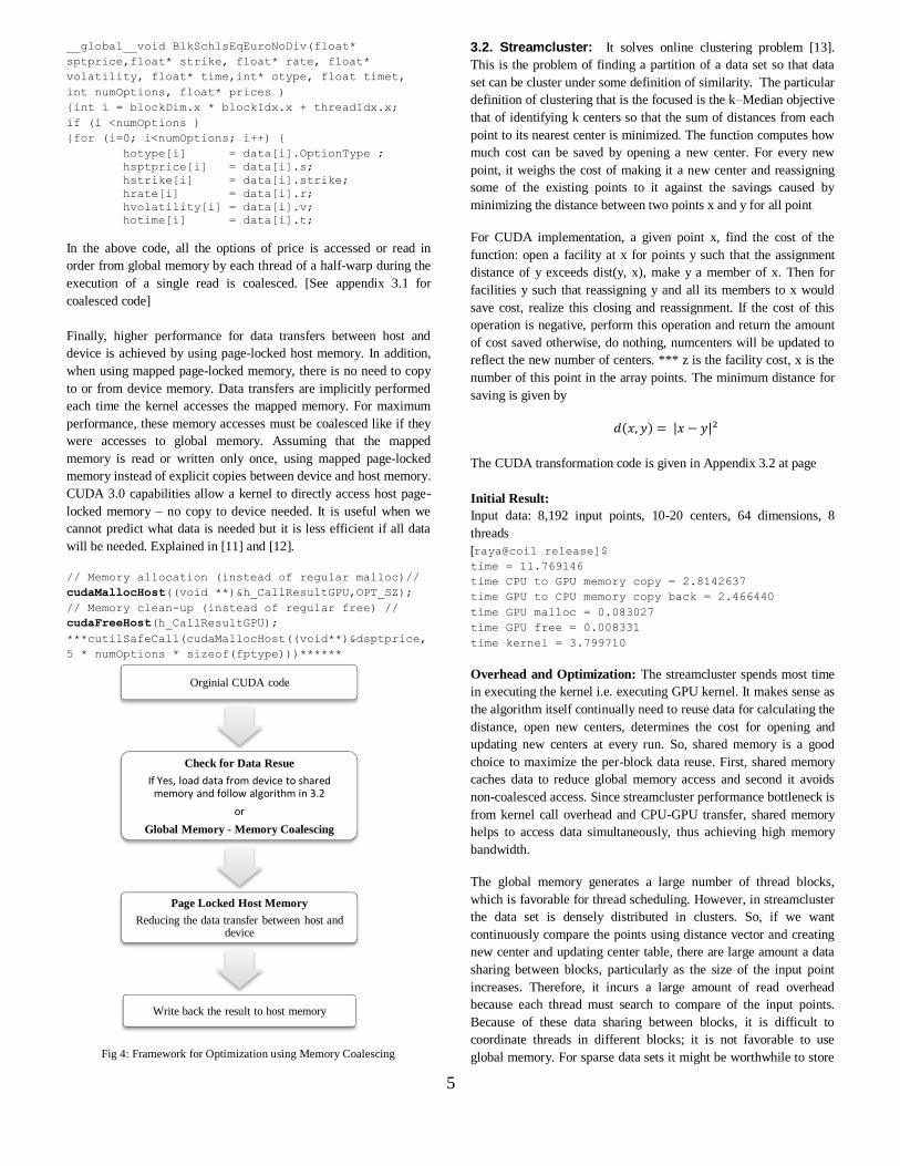
Fig 4: Framework for Optimization using Memory Coalescing

3.2. Streamcluster: It solves online clustering problem [13].

This is the problem of finding a partition of a data set so that data

set can be cluster under some definition of similarity. The particular

definition of clustering that is the focused is the k–Median objective

that of identifying k centers so that the sum of distances from each

point to its nearest center is minimized. The function computes how

much cost can be saved by opening a new center. For every new

point, it weighs the cost of making it a new center and reassigning

some of the existing points to it against the savings caused by

minimizing the distance between two points x and y for all point

For CUDA implementation, a given point x, find the cost of the

function: open a facility at x for points y such that the assignment

distance of y exceeds dist(y, x), make y a member of x. Then for

facilities y such that reassigning y and all its members to x would

save cost, realize this closing and reassignment. If the cost of this

operation is negative, perform this operation and return the amount

of cost saved otherwise, do nothing, numcenters will be updated to

reflect the new number of centers. *** z is the facility cost, x is the

number of this point in the array points. The minimum distance for

saving is given by

The CUDA transformation code is given in Appendix 3.2 at page

Initial Result:

Input data: 8,192 input points, 10-20 centers, 64 dimensions, 8

threads

[raya@coil release]$

time = 11.769146

time CPU to GPU memory copy = 2.8142637

time GPU to CPU memory copy back = 2.466440

time GPU malloc = 0.083027

time GPU free = 0.008331

time kernel = 3.799710

Overhead and Optimization: The streamcluster spends most time

in executing the kernel i.e. executing GPU kernel. It makes sense as

the algorithm itself continually need to reuse data for calculating the

distance, open new centers, determines the cost for opening and

updating new centers at every run. So, shared memory is a good

choice to maximize the per-block data reuse. First, shared memory

caches data to reduce global memory access and second it avoids

non-coalesced access. Since streamcluster performance bottleneck is

from kernel call overhead and CPU-GPU transfer, shared memory

helps to access data simultaneously, thus achieving high memory

bandwidth.

The global memory generates a large number of thread blocks,

which is favorable for thread scheduling. However, in streamcluster

the data set is densely distributed in clusters. So, if we want

continuously compare the points using distance vector and creating

new center and updating center table, there are large amount a data

sharing between blocks, particularly as the size of the input point

increases. Therefore, it incurs a large amount of read overhead

because each thread must search to compare of the input points.

Because of these data sharing between blocks, it is difficult to

coordinate threads in different blocks; it is not favorable to use

global memory. For sparse data sets it might be worthwhile to store

Orginial CUDA code

Check for Data Resue

If Yes, load data from device to shared memory and follow algorithm in 3.2

or

Global Memory - Memory Coalescing

Page Locked Host Memory

Reducing the data transfer between host and device

Write back the result to host memory

6

the dataset in cacheable constant memory, however for dense data

sets it could be difficult to find enough data points in range to

completely populate a warp, leading to performance degradation

from unutilized processors.

While CUDA does not provide a hardware-managed cache for

global memory, it is desirable to temporarily write the output

distance values to shared memory as they must be read multiple

times in each block and data reuse. However, CUDA does not

provide any cache for global memory. While the constant & texture

memory partitions are cacheable, these memories are read-only, and

thus cannot be used to store the output which accounts for half of all

memory references. So, shared memory is a good choice.

To overcome the lack of caching on the global memory, we use the

per-SM shared memory as a software-managed cache. In

streamcluster, a thread block is assigned to each point on the output

grid and reads from any input samples as a cache creates many

challenges for kernels in which data may be shared between

different thread blocks.

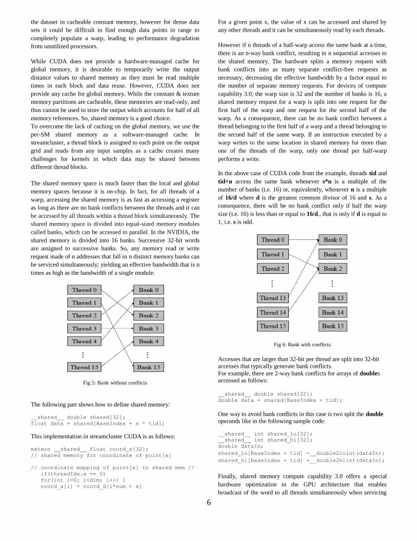
The shared memory space is much faster than the local and global

memory spaces because it is on-chip. In fact, for all threads of a

warp, accessing the shared memory is as fast as accessing a register

as long as there are no bank conflicts between the threads and it can

be accessed by all threads within a thread block simultaneously. The

shared memory space is divided into equal-sized memory modules

called banks, which can be accessed in parallel. In the NVIDIA, the

shared memory is divided into 16 banks. Successive 32-bit words

are assigned to successive banks. So, any memory read or write

request made of n addresses that fall in n distinct memory banks can

be serviced simultaneously; yielding an effective bandwidth that is n

times as high as the bandwidth of a single module.

Fig 5: Bank without conflicts

The following part shows how to define shared memory:

__shared__ double shared[32];

float data = shared[BaseIndex + s * tid];

This implementation in streamcluster CUDA is as follows:

extern __shared__ float coord_s[32];

// shared memory for coordinate of point[x]

// coordinate mapping of point[x] to shared mem //

if(threadIdx.x == 0)

for(int i=0; i<dim; i++) {

coord_s[i] = coord_d[i*num + x]

For a given point x, the value of x can be accessed and shared by

any other threads and it can be simultaneously read by each threads.

However if n threads of a half-warp access the same bank at a time,

there is an n-way bank conflict, resulting in n sequential accesses to

the shared memory. The hardware splits a memory request with

bank conflicts into as many separate conflict-free requests as

necessary, decreasing the effective bandwidth by a factor equal to

the number of separate memory requests. For devices of compute

capability 3.0, the warp size is 32 and the number of banks is 16, a

shared memory request for a warp is split into one request for the

first half of the warp and one request for the second half of the

warp. As a consequence, there can be no bank conflict between a

thread belonging to the first half of a warp and a thread belonging to

the second half of the same warp. If an instruction executed by a

warp writes to the same location in shared memory for more than

one of the threads of the warp, only one thread per half-warp

performs a write.

In the above case of CUDA code from the example, threads tid and

tid+n access the same bank whenever s*n is a multiple of the

number of banks (i.e. 16) or, equivalently, whenever n is a multiple

of 16/d where d is the greatest common divisor of 16 and s. As a

consequence, there will be no bank conflict only if half the warp

size (i.e. 16) is less than or equal to 16/d., that is only if d is equal to

1, i.e. s is odd.

Fig 6: Bank with conflicts

Accesses that are larger than 32-bit per thread are split into 32-bit accesses that typically generate bank conflicts.

For example, there are 2-way bank conflicts for arrays of doubles accessed as follows: __shared__ double shared[32];

double data = shared[BaseIndex + tid];

One way to avoid bank conflicts in this case is two split the double

operands like in the following sample code:

__shared__ int shared_lo[32];

__shared__ int shared_hi[32];

double dataIn;

shared_lo[BaseIndex + tid] =__double2loint(dataIn);

shared_hi[BaseIndex + tid] =__double2hiint(dataIn);

Finally, shared memory compute capability 3.0 offers a special

hardware optimization in the GPU architecture that enables

broadcast of the word to all threads simultaneously when servicing

7

one memory read request. This reduces the number of bank conflicts

when several threads of a half-wrap read from an address within the

same 32-bit word.

The CUDA transformation and optimization code is given in

Appendix 3.2 at page.

Fig 7: Framework for optimization using shared memory

3.3. Ferret: This application is based on the Ferret toolkit [15]

which is used for content-based similarity search of feature-rich data

such as audio, images, video, 3D shapes and so on. It is a search

engine which finds a set of images similar to a query image by

analyzing their contents. The input is an image database and a series

of query images. It involves breaking the images into segments in

order to distinguish different objects in the image. The segmented

images uses feature extraction which mathematically describe

content of segment. This is then indexed (selecting images that

matches the query images) and ranked (ranking according to order

of similarity). The four stages involving ferret are query image

segmentation, feature extraction, indexing of candidate sets with

hashing and ranking using with finding nearest neighbor search

using distance vector algorithm.

Segmentation is the process of decomposing an image into separate

areas which display different objects. The rationale behind this step

is that in many cases only parts of an image are of interest, such as

the foreground. Segmentation allows the subsequent stages to assign

a higher weight to image parts which are considered relevant and

seem to belong together.

After segmentation, ferret extracts a feature vector from every

segment. A feature vector is a multi-dimensional mathematical

description of the segment contents. It encodes fundamental

properties such as color, shape and area. Once the feature vectors

are known, the indexing stage can query the image database to

obtain a candidate set of images. This method uses hash functions

which map similar feature vectors to the same hash bucket with high

probability. It then employs a step-wise approach which indexes

buckets with a higher success probability first. After a candidate set

of images has been obtained by the indexing stage, it is sent to the

ranking stage which computes a detailed similarity estimate and

orders the images according to their calculated rank. The similarity

estimate is derived by analyzing and weighing the pair-wise

distances between the segments of the query image and the

candidate images. For a given query image X and database image Y,

the ferret employs the Earth Mover’s Distance (EMD) given by

)

To implement this algorithm in CUDA, we took the original ferret-

parallel.c from the Parsec 2.1 ferret and then we assign the distance

calculation of each data point to a single thread for analyzing and

weighing the minimum distances between the segments of the query

image and the candidate images using blocks of thread in parallel.

Then the distance for each test point was sorted in parallel.

Therefore each thread loop over all the initial stored data,

calculating its assigned data point’s distance with query data,

finding the minimum distance from its data point to a stored images

using feature extraction for best match and filtering out the few

matches. When all threads are finished doing this, the membership

of each data point is known, copy result back from GPU to CPU.

Result:

[raya@coil release]$ ferret

Throughput = 31.45 GB/s, Time = 12.11s, Size =

35000 threads = 32

CPU-GPU Transfer Time = 5.71s

Calculating the distance = 3.23s

Filtering = 1.04s

Overhead and Optimization: The GPU-based implementation of

ferret is clearly memory bound as there is more memory access. The

algorithm for this pass requires intensive data sharing, and creates

congestion on the memory subsystem. For example, one possible

way of parallelizing this pass is to ask all threads whose data point

belongs in a same group to add their values to a certain data

structure in memory.

Ferret is good candidate of shared memory as ferret needs to access

only the values in a correlated section of memory. In ferret,

calculating distance means we need to load the current image to find

the distance between the already stored images to find the best

possible match. So, all the treads within the block calculate the

distance. For memory throughput, the time for CPU-GPU transfer

and the GPU execution holds equally for overheads. When this is

the case, shared memory becomes the most effective memory to use.

Load data from device memory to shared memory

Synchronize with all the other threads of the block so that each thread can safely read

shared memory locations

Process the data in shared memory

Optimization:

• When no bank conflicts- Shared Memory accessed by all threads within a thread block simultaneously providing servicing to different request made on different banks

• But, when blank conflicts occur - Splits the bank into one request for first half of the warp and then to one request for the second wrap

• When many read request comes to same bank, broadcast to all threads simultaneously

Synchronize again to make sure that shared memory has been updated with the results

Write back the result to device memory

8

Shared memory allows all threads within a block to share

information. First, data is read from global memory into shared

memory (accessing the images to calculate the distance in each

threads and finding which one is the best match), ensuring that

consecutive threads in a half-warp read from consecutive memory

addresses to facilitate non coalesced memory access. Then

calculations are performed using only shared memory. Finally, the

results are written to global memory. The general shared memory

optimization implementation is same as we did in streamcluster

avoiding all bank conflicts. Here initially, we compute the distance

and filtered and stored matched images in shared memory. The

process was repeated several times till we get the top 10 images and

finally this top 10 images is stored in global memory. Here, we are

explicitly using shared memory because just we dividing kernel into

global memory for flushing the data and reading the data into shared

memory and storing the value of kernel call arguments could cause

for extra overhead due to limit in resources of 16KB of shared

memory and limited registers. Any bank conflict in shared memory

is eliminated in same way as the streamcluster.

3.4. Swaptions: A financial analysis application to price the

portfolio of the swaptions. It solves a PDE equation and stores the

portfolio in swaptions array. The swaptions application uses the

Heath-Jarrow-Morton (HJM) framework [18] to price a portfolio of

swaptions. The HJM framework describes how interest rates evolve

for risk management and asset liability management for a class of

models between the option seller and the option buyer whereby the

option buyer is granted a right secured by the option seller, to carry

out some operation at some moment in the future. Its central insight

is that there is an explicit relationship between the drift and

volatility parameters of the forward-rate dynamics in a no arbitrage

market. Swaptions therefore employs Monte Carlo (MC) simulation

to compute the prices. The program stores the portfolio in the

swaptions array. Each entry corresponds to one derivative.

Swaptions partitions the array into a number of blocks equal to the

number of threads and assigns one block to every thread.

The price of the underlying options with constant drift µ and

volatility (where Wt is Wiener random

process). Details of the equation given in [18].

For CUDA implementation, swaptions array is partitioned into

number of work units threads and processed concurrently. Device

memory is allocated to run compute to price. Each thread block is

iterated and calls for HJM Swaption Blocking function for every

entry to compute prices. It generates a random HJM path for each

run. Once the path is generated, we compute the value of swaptions

(expected value and confidence width). Each thread computes and

sums the multiple simulation paths and stores the sum and the sum

of squares into a device memory. The number of option computed is

one option per thread. Then, computed sum is put back to the host

memory.

float r = d_Random[pos];

float endStockPrice =S*__expf(MuByT+BySqrtT * r);

float callProfit = fmaxf(endStockPrice - X, 0);

sumCall.Expected += callProfit;

sumCall.Confidence += callProfit * callProfit

Initial Result: [raya@coil release]$

Options : 256

Simulation paths: 14100

Time (ms) : 6.45204

Kernel = 1.17525

CPU to GPU memory = 2.142637

GPU to CPU memory = 1.766440

Overhead and Optimization: The swaptions generates a HJM path

after being implemented in CUDA and we use them to compute an

expected value and pricing for the underlying option. There are

multiple ways we could go about computing the mean of all of the

samples. The number of options is typically in the hundreds or

fewer, so computing one option per thread will likely not keep the

GPU efficiently occupied. Therefore, we concentrate on using

multiple threads per option. Given that, we have two choices; we

can either use one thread block per option, or multiple thread blocks

per option or we can use combination of both. When computing a

very large number of paths per option, it will probably help us to

reduce the latency of reading the random input values if we divide

the work of each option across multiple blocks.

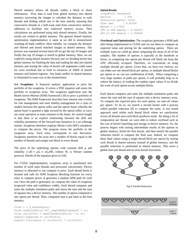
Each thread computes and sums the multiple simulation paths and

stores the sum and the sum of squares into a device memory array.

To compute the expected price for each option, we sum all values

per option. To do so, we launch a second kernel with a process

called parallel reduction [8] to compute the sums. A tree based

approach used within each thread block where we synchronize

across all threads once each block produces result. By doing a lot of

computation per thread, we were able to reduce overhead such as

the cost of kernel launching and storage to device memory. So, the

process begins with storing intermediate results of the options to

global memory, finish the first kernel, and then launch the parallel

reduction kernel to compute the final sum. Indeed, we compute

these final values using a single thread block per option by storing

each thread in shared memory instead of global memory, and the

parallel reduction is performed in shared memory. This saves a

global store per thread and an extra kernel invocation.

Fig 8: Parallel Reduction

9

The CUDA code for Parallel reduction for Address Interleaving: global__ void reduction(float *g_data, int n) {

__shared__ float sdata[blocksize];

// each thread loads one element from global to

shared memory

unsigned int tid = threadIdx.x;

unsigned int i = blockIdx.x*blockDim.x

threadIdx.x;

if(i<n){sdata[tid]=g_data[i];}

// do reduction in shared memory

for(unsigned int s=1; s < blockDim.x; s *= 2)

{if (tid % (2*s) == 0) {

sdata[tid] = max(sdata[tid], sdata[tid + s]);

// write result for this block to global memory

if (tid == 0) g_odata[blockIdx.x] = sdata[0];

Fig 9: Calculating value in Parallel Reduction

The optimized CUDA is written in swaptions_reduction file.

__device__ void sumReduceSharedMem(volatile T *sum,

volatile T *sum2, int tid)

{

// do reduction in shared mem

for(unsigned int s=1;s<blockDim.x;s*= 2)

{if (tid % (2*s) == 0) {

sum[tid] = max(sum[tid], sum[tid + s]);

if (blockSize >=512){if(tid< 256){sum[tid]+=sum[tid

+ 256];sum2[tid]+=sum2[tid +256]; }

__syncthreads(); }

if (blockSize >=256){if(tid <128){sum[tid]+=sum[tid

+128];sum2[tid]+=sum2[tid +128]; }

__syncthreads(); }

if (blockSize >= 128){if(tid <64){sum[tid]+=sum[tid

+ 64];sum2[tid]+=sum2[tid + 64]; }

__syncthreads(); }

#ifndef __DEVICE_EMULATION__

if (tid < 32)

#endif

{

if (blockSize >= 64) { sum[tid] += sum[tid + 32];

sum2[tid] += sum2[tid + 32]; EMUSYNC; }

if (blockSize >= 32) { sum[tid] += sum[tid + 16];

sum2[tid] += sum2[tid + 16]; EMUSYNC; }

if (blockSize >= 16) { sum[tid] += sum[tid + 8];

sum2[tid] += sum2[tid + 8]; EMUSYNC; }

if (blockSize >= 8) { sum[tid] += sum[tid + 4];

sum2[tid] += sum2[tid + 4]; EMUSYNC; }

if (blockSize >= 4) { sum[tid] += sum[tid + 2];

sum2[tid] += sum2[tid + 2]; EMUSYNC; }

if (blockSize >= 2) { sum[tid] += sum[tid + 1];

sum2[tid] += sum2[tid + 1]; EMUSYNC; }

So, the improvement allows easier loading of value and calculating

the sum in parallel reduction with shared memory and parallel

loading of data from global to shared memory, writing back to

subsequent addresses. Further, we used loop unrolling to reduce the

instruction overhead. Loop Unrolling is a technique in which the

body of a suitable loop is replaced with multiple copies of itself, and

the control logic of the loop is updated accordingly. Reducing the

number of blocks to half by performing two loads and add instead of

single load, replacing load/add with multiple add, we optimize it

further. The details how we select optimal loop unroll factors for

loop in GPU program is explained in [19]. The loop unrolling

doesn’t provide huge improvement but a significant amount

improvement has been achieved. If the loop unrolling resulted in

fetch/store coalescing then a big performance improvement could

result.

#ifdef UNROLL_REDUCTION

sumReduceSharedMem<T, blockSize>(sum, sum2, pos); }

#else

for(int stride=SUM_N/2; stride > 0; stride >>= 1){

__syncthreads();

for(int pos = threadIdx.x; pos < stride; pos +=

blockSize){

sum[pos] += sum[pos + stride];

sum2[pos] += sum2[pos + stride];

unsigned int tid = threadIdx.x;

unsigned int i = blockIdx.x * (blockDim.x * 2) +

threadIdx.x;

sum[tid] = max(sum[i], sum2[i + blockDim.x]);

3.5. x264: The x264 application is an H.264/AVC (Advanced

Video Coding) video encoder. H.264 describes the lossy

compression of a video stream [13] which provides many improved

features. The advancements allow H.264 encoders to achieve a

higher output quality with a lower bit-rate. The flexibility of H.264

allows its use in a wide range of contexts with different

requirements, from video conferencing solutions to high-definition

(HD) movie distribution. Next generation HD DVD or Blu-ray

video players already require H.264/AVC encoding. H.264 encoders

and decoders operate on macroblocks of pixels which have the fixed

size of 16×16 pixels. Various techniques are used to detect and

eliminate data redundancy. The most important one is motion

estimation process [9]. Motion compensation is usually the most

expensive operation that has to be executed to encode a frame.

Motion estimation algorithm exploits redundancy between frames,

which is called temporal redundancy. A video frame is broken down

into macroblocks (each macroblock typically covers 16×16 pixels),

each macroblock’s movement from a previous frame (reference

frame) is tracked and represented as a vector, called motion vector.

Storing this vector and residual information instead of the complete

pixel information greatly reduces the amount of data used to store

the video.

Motion Estimation is the process of finding the lowest cost (in bits)

way of representing a given macroblock’s motion. In video, pixel

values often do not change much across scenes (frames), and the

pixel values of a block can be predicted from the values of a similar

block in a previous frame (reference frame). The motion estimation

operates to find a motion vector, which indicates the similar block in

the reference frame, and residuals to compensate prediction errors.

10

To find the motion vector, the motion estimation algorithm finds the

best match in a certain window of the reference frame. The block

coded with motion estimation is called inter-coded. This fact is used

to aid in the compression process. Rather than transmitting the

entire motion vector for a given macroblock, we only need to

transmit how it differs from what we predict it would be, given how

the blocks around it moved. The motion vector prediction (MVp) is

the median of these three vectors. We only need to transmit how a

given block’s motion vector differs from the MVp. To do that they

account the cost of encoding the residual as well as the cost of

encoding the motion vector as a prime area of estimating cost. In

order to solve the problem of performing motion estimation in a

massively parallel environment we needed to deal with the issue of

needing the MVp to find the optimal motion vector. The whole

explanation is beyond the scope of this project. Please refer paper

[20] and [21] for further details.

For CUDA implementation of x264, we used global memory for

part of input data, since data use has 2D locality. x264 required

more modification when imported to CUDA, involved large scale

code transformation from the Parsec parallel application code. In

CUDA, the problem of needing the MV is solved by properly

estimating the cost of a given motion vector by using an estimate of

what the MVp will actually be like. This cost calculation uses a

evaluation metrics called Sum of Absolute transferred difference

[refer wikipedia]: cost=SATD+[C(MVx−MVpx)+C(MVy−MVpy)]

where C(.) is the cost of encoding a motion vector differential of

that length. In our implementation, a macroblock is divided into

sixteen 4x4 blocks, and the SAD value of each 4x4 block is

calculated in parallel for all candidate motion vectors (positions)

within the search range on the reference frame. We then merge these

4x4 block SADs to form the 4x8, 8x4, 8x8, 8x16, 16x8, and 16x16

block SADs, respectively. For each block size, we compare the

SADs of all candidate MVs and the one with the least SAD is the

integer-pixel motion vector (IMV), MV with integer pixel accuracy.

Next, in order to obtain the fractional pixel motion vectors, the

reference frame is interpolated using a filter as defined in the

H.264/AVC standard. We calculate the SADs at 24 fractional pixel

positions that are adjacent to the best integer MV, and then choose

the least SAD position as the fraction-pixel motion vector (FMV).

Now one block per macroblock is assigned. We had one thread

check each search position within the search window. By having

one block per macroblock we were able to take advantage of thread

synchronization to perform a reduction to find the lowest cost

motion vector for each macroblock.

Initial Result: [raya@coil release]$x264 Loaded 'pixel_size.pgm',

„640 x 340 pixels‟

Processing time: 0.118000s

81.56 pixels/sec

GPU execution = 0.0306800s

CPU-GPU transfer = 0.0631000s

Overhead and Optimization: Our implementation of x264 is

bounded by both GPU execution and CPU-GPU transfer but it looks

like GPU-CPU communication holds for overhead in overall

computation time than GPU execution. While x264 CUDA

implementation does not take advantage of shared memory to

preload the needed pixel values, it does store both the current frame

and the reference (previous) frame in global memory. So, x264

regularly need to access neighboring memory locations with 2D

spatial locality, using texture memory instead of global memory is

useful for performance increase. Global memory doesn’t provide

caching; it is desirable to use texture memory. Reading device

memory through texture fetching present some benefits that can

make it an advantageous alternative to reading device memory from

global or constant memory:

If the memory reads do not follow the access patterns that

global or constant memory reads must respect to get good

performance, higher bandwidth can be achieved providing that

there is locality in the texture fetches.

Addressing calculations are performed outside the kernel by

dedicated units.

Packed data may be broadcast to separate variables in a single

operation.

Now, every multiprocessor on a GPU has its own texture cache,

originally designed for storing images that are reproduced many

times to create the illusion of a textured object. Tesla T1 provides

support for special optimized texture transformation operations with

texture memory upto size of global memory which the largest size

among all memories and clock cycle of > 100 cycles. This extra

support comes at the cost of higher latency than constant memory

for normal read operations. Whenever an element of the texture data

type is read from global memory it is stored in the texture cache on

the device, and all subsequent requests for this element do not need

to read from global memory. As texture memory space resides in

device memory and is cached in texture cache, so a texture fetch

costs one memory read from device memory only on a cache miss,

otherwise it just costs one read from texture cache. The texture

cache is optimized for 2D spatial locality, so threads of the same

warp that read texture addresses that are close together in 2D will

achieve best performance. Also, it is designed for streaming fetches

with a constant latency; a cache hit reduces DRAM bandwidth

demand but not fetch latency. While the constant & texture memory

partitions are cacheable, these memories are read-only, and thus

cannot be used to store the output which accounts for half of all

memory references. As, in x264, we need to predict the successive

blocks depending on the previous block, it is important to store the

output partially somewhere. So, we used shared memory as a good

option as all the threads within a specific block are able to share

information. All of the main calculations used for processing occur

within shared memory, and then all of the results are transferred to

texture memory.

// declare texture reference for 2D float texture//

texture<uint8_t,2,cudaReadModeElementType>

currentTex;

Initially, when the pixel size is small, 16834 register was enough for

SAD calculation in texture but with large pixel size and frame a lack

of registers restricts the number of threads that could be scheduled,

exposing the latency of texture memory. We also achieve potential

throughput using loop unrolling. Loop unrolling is the most

common optimization in compiler construction. Loop unrolling

reduces the operations which is not part of core data computation.

By unrolling the X loop by 4, we can compute MVx, MV px, MVy,

MVpy once and use it multiple times, much like the CPU version of

11

the code does Doing this will not affect shared memory usage and a

register is saved by removing the unrolled loop’s induction variable.

The following code shows for shared memory usage and loop

unrolling in x264:

__shared__ float As[16][16];

__shared__ float Bs[16][16];

// load input tile elements

As[MVx][MVy] = A[indexA];

Bs[MVpx][MVpy] = B[indexB];

indexA += 16;

indexB += 16 * widthB;

__syncthreads();

// compute results for tile

Ctemp += As[MVx][0] * Bs[0][MVy];

Ctemp += As[MVpx][15] * Bs[15][MVpy];}

__syncthreads();

C[indexC] = Ctemp;

__device__ unsigned mvCost(int dx, int dy){

//loop unrolling//

float dx1 = (abs(dx))<<2;

float dx2 = (abs(dx))<<2;

float dx3 = (abs(dx))<<2;

float dx4 = (abs(dx))<<2;

int x1Cost=round((log2f(dx+1)*2+0.718f+!!dx)+ .5f);

int x2Cost=round((log2f(dx+1)*2+0.718f+!!dx)+ .5f);

int x3Cost=round((log2f(dx+1)*2+0.718f+!!dx)+ .5f);

int x4Cost=round((log2f(dx+1)*2+0.718f+!!dx)+ .5f);

3.6. Fluidanimate: This Intel RMS application uses an extension

of the Smoothed Particle Hydrodynamics (SPH) method to simulate

an incompressible fluid for interactive animation purposes [22]. Its

output can be visualized by detecting and rendering the surface of

the fluid. The force density fields are derived directly from the

Navier-Stokes equation which is written as follows:

where v is a velocity field, is a density field, p a pressure field, g

an external force density field and μ the viscosity of the fluid.

The density at a location r can be calculated by equation:

Applying the SPH interpolation equation to the pressure term and

the viscosity term of the Navier-Stokes equation yields the

equations for the pressure and viscosity forces

For CUDA implementation, it follows same principle as

blackscholes each parameters like velocity field, density field,

pressure field, external force density field and viscosity of the fluid

are computed in device memory with threads and the final value is

again copied back to host memory. All the functions use global

memory. The fluidanimate represents in 3D version for node nx, ny

and nz which are the number of computational nodes in the x, y and

z directions for a flow domain, respectively. The 3D domain of size

nx× ny ×nz is represented by a breadth nx, width nx and height nz

on the host side.

// number of grid cells in each dimension

int nx, ny, nz;

// cell dimensions

struct Vec3 delta;

Fig 10: Dimensional array x, y, z

On the GPU side, the representation is used to store data in global

memory. This 3D mapping translates to efficient data transfer

between the host and the device. Several matrices are needed to

represent the pressure and velocity components at different time

levels. Memory allocation on the device is done only once before

starting the time stepping. In our implementation, the velocity field

at time t depends only on the velocity field at t-1. Five different

matrices are used to represent the velocity fields. The matrices are

swapped at the end of each time step for reuse GPU code is of five

different kernels to implement the steps of the algorithm:

Rebuild spatial index Because the smoothing kernels W(r − rj,h)

have finite support h, particles can only interact with each other up

to the distance h. The program uses a spatial indexing structure in

order to exploit proximity information and limit the number of

particles which have to be evaluated.

__device__ void RebuildGridMT(int i, int nx, int

ny, int nz, struct Vec3 delta, bool* border, Cell*

cells, Cell* cells2, int* cnumPars, int* cnumPars2,

Grid* grids)

Compute densities This kernel estimates the fluid density at the

position of each particle by analyzing how closely particles are

packed in its neighborhood. In a region in which particles are

packed together more closely, the density will be higher.

_device__void ComputeDensities2MT(inti,float

hSq,float densityCoeff,int nx,int ny,bool* border,

Cell* cells, Cell* cells2, int* cnumPars, int*

cnumPars2, Grid* grids)

Compute forces Once the densities are known, they can be used to

compute the forces. The kernel evaluates pressure, viscosity and

also gravity as the only external influence.

__device__void ComputeForcesMT(int i,float h,float

hSq,float pressureCoeff,float viscosityCoeff,int

nx, int ny, int nz, bool* border, Cell* cells int*

cnumPars, int* cnumPars2, Grid* grids)

12

Handle collisions with scene geometry The next kernel updates the

forces in order to handle collisions of particles with the scene

geometry. __device__void ProcessCollisionsMT(int i,int nx,int

ny,bool* border,Cell* cells,Cell* cells2 int*

cnumPars, int* cnumPars2, Grid* grids)

Update positions of particles Finally, the forces can be used to

calculate the acceleration of each particle and update its position.

Result:

Particles size: 100K

[raya@coil release]$ fluidanimate,512 Throughput

= 8.3400 GB/s, Time = 0.005972 s, Size = 100000

Time transfer CPU to GPU = 0.001998 s

GPU Kernel execution = 0.002252 s

Time transfer GPU to CPU = 0.001737 s

Overheads and Optimization: Fluidanimate uses 5 kernels, 2 of

which are further divided into further parts, has peak memory

throughput of approximately 10.450 GB/sec, which corresponds to

an optimal balance of just over 5 math operations per double

precision value loaded from memory. Because most of loops

perform a large amount of math, performance of code is mainly

limited by memory bandwidth. The throughput is limited because of

the global memory access for all 5 kernels. For the above domain,

each GPU needs neighboring data computed by other GPUs which

means all GPUs need to synchronize to exchange velocity and

pressure fields at each time step. But a GPU cannot directly

exchange data with another GPU. Hence, cells at the GPU domain

decomposition boundaries needs to be copied back to the host,

which adds an extra communication overhead to the overall

computation in addition to the CUDA kernel launches at every time.

For Optimization, if threads in a warp read from the same cache line

in the same cycle, these reads are batched into a single operation via

a process known as memory coalescing for global memory which

helps conserve bandwidth while reducing effective latency,

therefore speedup the whole program. The concept is similar to

loading an entire cache line from memory versus loading one word

at a time at CPU. Coalescing operates at half-warp granularity, so

uncoalesced loads and stores waste approx. 15/16ths of available

memory bandwidth. Therefore the most important optimization for

memory-bound applications is to arrange work so that threads in the

same warp will access sequential memory locations at the same

time. However, since 5 kernel runs at the same time, not all threads

participated in coalescing. It is important to divide the memory

coalesced access and non-coalesced access. For the non-coalesced,

the access is benefited by using shared memory. 2 or 3 kernels can

be used for the shared memory which involves data reuse and

updates high arithmetic intensity. This will reduce the overhead and

increase performance due to data transfer to the shared memory is

largely compensated by this high arithmetic intensity.

CUDA optimization algorithm

Coalesced the global memory access. The simultaneous global

memory accesses by each thread of a half-warp during the

execution of a single read or write instruction will be coalesced

into a single access if:

The size of the memory element accessed by each thread

is either 4, 8, or 16 bytes

The elements form a contiguous block of memory

The Nth element is accessed by the Nth thread in the half-

warp

The address of the first element is aligned to 16 times the

element’s size

Read from the input of the global memory and copy the sub-

domain from the global memory to the shared memory.

Computation done by the threads, using data from the shared

memory and write to the shared memory.

Read from shared memory and the final result of the

computation is written back to the global memory before

exiting the kernel.

This back and forth data transfer between the global memory to the

shared memory creates an overhead. But due to high arithmetic

intensity of the kernel the overhead of data copying in order to

benefit from the shared memory implementation.

3.7. Raytrace: The raytrace application is an Intel RMS workload

which renders an animated 3D scene. Ray tracing is a technique that

generates a visually realistic image by tracing the path of light

through a scene. Rays through each pixel in an image plane are

traced back to the light source. The scatter model describes what

happens when a ray hits a surface. Raytracing works by projecting a

ray of vision through each pixel on the screen from the observer.

When the rays through the screen intersect an object, it is projected

onto the screen. For every pixel on the screen, an equation involving

the ray through that pixel from the observer and each object in the

scene is solved to determine if the ray intersects the object. Then,

the pixel through which the ray passes is set to the color of the

intersected object at the point of intersection. If more than one

object is intersected, then the closer of the intersections is taken.

Reflections and shadows are achieved through what is known as

recursive ray tracing. When figuring out the color of the

intersection, one important factor is whether that point is in shadow

or not. To find this out, the same techniques are used, but instead of

the normal location of the observer, the ray starts at the point of

intersection and moves toward any light sources. If it intersects

something, then the point is in shadow. When a reflective Surface is

intersected, a new ray is traced starting from the point of

intersection. The color that this ray returns is incorporated into the

color of the original intersection.

Fig 11: Raytracing method

13

Finding intersection points follows raytracer storage of the scene

graph in a Bounding Volume Hierarchy (BVH). A BVH is a tree in

which each node represents a bounding volume. The bounding

volume of a leaf node corresponds to a single object in the scene

which is fully contained in the volume. Bounding volumes of

intermediate nodes fully contain all the volumes of their children, up

to the volume of the root node which contains the entire scene. If the

bounding volumes are tight and partition the scene with little

overlap then a ray tracer searching for an intersection point can

eliminate large parts of the scene rapidly by recursively descending

in the BVH while performing intersection tests until the correct

surface has been found.

Fig 12: Raytracing algorithm for bounding volume hierarchy

For CUDA implementation, BVH uses a transversal algorithm[17]

The BVHs is built in top-down fashion with surface area heuristics

using the centroids of bounding boxes for scene triangles, tracing

packets of rays and only the node address is saved to the stack. As a

BVH does not need to store the mint and maxt values along the ray,

only the node address is saved to the stack. The algorithm maps one

ray to one thread blocand a packet to a chunk. It traverses the tree

synchronously with the packet and work on one node at a time and

process whole packet against it. If the node is a leaf, it intersects the

rays in the packet with the contained geometry. Each thread stored

the distance to the nearest found intersection. If the node is not a

leaf, the algorithm loads the two children and intersects the packets

with both of them to determine the traversal order. Each ray

determines which of the two nodes it intersects and in which it

wants to go first by comparing the signed entry distances of both

children. For packet traversal, the stack can be shared by all the

threads in a packet, which increases the utilization of the resources.

The order of traversal among several threads is resolved by a

concurrent write to the shared memory. Each thread then writes the

preference to one of four entries, value one for one of the four cases:

traverse left, traverse right, traverse both, and traverse none. If at

least one ray wants to visit the other node then the address of this

other node is pushed onto stack. In case all rays do not want to visit

both nodes or after the algorithm has processed a leaf, the next node

is taken from the top of the stack and its children are traversed. If

the stack is empty, the algorithm terminates.

Initial Results and Optimization:

[raya@coil release]$ raytrace “loading scene”

“512 x 512 pixels”

Time = 21.5672 s

5. Experimental Results:

In this part of the section we calculated the execution time

theoretically to match it with experimental value and check the

degree of the correctness.

As we calculated the speed up percentage for transformation from

CPU to GPU and from GPU original to GPU optimized.

We check the experimental value while running the CUDA program

on GPU. And then we spilt the time into various parts or into

various run to check the time taken by individual part to execute the

code. We calculated the execution time for the CUDA code without

optimization. This time division helped us to look for overhead in

the code and thus we were able to reduce or eliminate that

bottleneck with optimization in the description above. The initial

results for CUDA run without optimization is given in each

benchmark above.

Now, Let tgpu is the execution time for running the kernel on gpu,

tcpu_transfer is the time taken for transfer from cpu to gpu i.e. from

host to device, tgpu_transfer is the time taken to copy from gpu to cpu,

tgpu_alloc be the time for gpu memory allocation and tgpu_free is the

time taken for gpu memory free

The total time taken to execute the CUDA code:

ttotal = tcpu_transfer + tgpu + tgpu_transfer + tgpu_alloc + tgpu_free

Although Gpu memory allocation and gpu memory free accounts

for very less time, we can ignore the them in our calculation. To,

show an example we took the execution time from blackscholes. It

shows total executed time against the individual executed time. And

we calculated the theoretical value as below:

Blackscholes:

Size = 13200 options, threads = 512

Throughput = 1.4260 GOptions/s,

Time = 0.443 ms

Time transfer CPU to GPU = 0.197 ms

GPU Kernel execution = 0.0125 ms

Time transfer GPU to CPU = 0.2334 ms

Calculation:

Total execution time (ttotal) = 0.443s [Experimental result]

Theoretical results: ttotal = tcpu_transfer + tgpu + tgpu_transfer

= 0.1871 + 0.0125 + 0.2134 = 0.413ms

14

So, the theoretical value and the experimental value is

approximately same which proves our correctness of the program.

The little time difference is because of may be some other time like

the time taken for memory allocation, memory free and other

calculation. Calculating all these is beyond our scope of the project.

Table1: The following table showing the experimental time and calculated

theoretical time for each application:

Benchmarks Experimental Value

Theoretical Value

Blackscholes 0.443ms 0.413ms

Streamcluster 8.360s 8.134s

Ferret 11.21s 10.683s

Swaptions 8.39ms 8.26ms

x264 51.1ms 44.5ms

Fluidanimate 7.69ms 7.35ms

Raytrace 21.56 s 18.45s

The Speed up equation of CUDA execution time is given by,

Between CPU and GPU:

Between GPU original and GPU optimized:

Note: Look for 4.29(a) at page 16 performance comparison between CPU

and GPU.

Note: Look for 4.29(b) at page 17 performance comparisons between GPU

original and GPU optimized.

The speed takes in account the best gain obtained while running the

code in CPU and then in GPU. It is the time difference between the

execution time of CPU and GPU when it is maximum.

Eg, For Blackscholes with 65K size and 256 threads

CPU time = 4.265 ms and GPU time = 1.539

The following graphs shows the speed up percentage gained in GPU

against the speed up percentage the application is expected to

achieve when it is transformed to GPU platform.

Graph 1: Speed up comparison between original speed up, optimized speed

up and expected speed up. The speed is in percentage.

Similarly, we calculated the speed up from GPU original to GPU

optimized and checked how much gained performance speed up is

achieved in optimizing the CUDA code.

Benchmarks Speed Up Percentage

Blackscholes 41.66%

Streamcluster 48.63%

Ferret 23.93%

Swaptions 29.45%

x264 39.21%

Fluidanimate 45.4%

raytrace -

Table 2: Speed up from GPU original to GPU optimized

Graph 2: CPU-GPU Communication time between original CUDA and

optimized CUDA

6. Discussion:

While reader can draw his/her conclusion from experimental results

below, let us provide our interpretation of the measured data.

Application running on GPU has benefited from the degree of

parallelism available on GPU than CPU. Each application with

different size of inputs has shown great performance increase.

64.3

41.4 37.6

60.8

17.9

69.4

45.6

91.4

64.4

44.1

78.3

25.3

93.8

45.6

129

70 70

149

35

110

85

0

20

40

60

80

100

120

140

160

Orginial Speed Up Optimized Speed Up Expected Speed

1.784

5.2165.71

3.908

6.31

3.7

0.948

3.16

4.34

2.44

4.21

2.02

0

1

2

3

4

5

6

7

blackscholes (ms)

streamcluster (s)

ferret (s) swaptions (ms)

x264 (ms) fluidanimate (ms)

Original CUDA Optimized CUDA

15

Initially for small size of input the GPU execution time was same as

CPU. But as we increased the size of the input, the performance

became better and better. Also, Exploiting large number of threads

was the major factor for speed up. Application like blackscholes and

fluidanimate didn’t show much improvement but once the size of

input increased they out performed CPU showing 64.3% and 79.4%

of speed up which is good considering it was optimized later. And

application like swaptions, ferret showed improvement from the

beginning but we were unable to exploit the large number of threads

for some reason. The best one remains the x264 which achieved

improvement much closer as expected, achieving 17.9% against the

expected value of 50%. All these application achieved a speed up

without optimization.

Optimization helped the original code to rearrange the CUDA and

use some techniques to improve and achieve desirable speed to be

much closer to expected speed. Table 2 shows the speed up

percentage for the optimized code. It was interesting to see none of

application except one fluidanimate crossed speed more than 50%

and streamcluster which came closer to 50%. This may be due to the

fact that we did optimization purely on the GPU side adding extra

features from NVIDIA compute capability 3.0, changing and

rearranging the original code and making computational changes.

But, we never tried to change anything in the algorithm part of

application. Many papers implement their experimentation not only

for CUDA code optimization but also changing the algorithm to see

how it performs. This change is beyond our scope of the project. So,

the performance in table 2 is reasonable considering we

implemented original algorithm without any change.

Optimization like memory coalescing with input size from 50K -

100K reduces the running time dramatically for fluidanimate and

blackscholes. For input size at 100K, the running time under

memory coalescing for fluidanimate is 50% lower than that of

original kernel execution. But for input size at 3K, 15K and 300K,

the effects of memory coalescing is not as large at others. Since for

this application, we only modified a portion of the data to obtain

memory coalescing, the speedup could be larger if we apply the

modification to every portion of the code which impossible

manually. Optimization like shared memory worked well for

streamcluster for 4K and 8K size but didn’t affect much for ferret

and swaptions. Also, optimization like parallel reduction in

swaptions didn’t work really well as expected. Again, x264

performed well for texture memory, shared memory and loop

unrolling optimization. There are several other optimization as we

do in compiler construction but it is impossible to apply them

manually on CUDA and check the performance.

6. Conclusion and Future Work:

In this project, we presented the parallelized CUDA code of Parsec

application for blackscholes, streamcluster, ferret, swaptions, x264,

fluidanimate and raytrace respectively. This paper characterized the

applications in terms of inherent algorithm characteristics,

parallelization, overhead, and optimization, and showed that each

application exhibits unique characteristics. We presented efficient

optimization like memory coalescing, bank conflict shared memory,

cached texture memory, loop unrolling, parallel reduction and

demonstrated that the GPU acting as a coprocessor can effectively

accelerate massive data computation. Experimental results show that

with GPU, the process is 4-6 times faster than the CPU only

configuration. And also our experimental result show that optimized

kernel functions greatly outperform the naive kernel functions. Our

future work extending Parsec benchmark to support more platforms,

such as FPGAs.

7. Reference: 1) http://developer.download.nvidia.com/compute/cuda/sdk/website/samp

les.html.

2) NVIDIA CUDA. http://developer.nvidia.com/object/cuda.html

3) GPUPU Programming lecture by David Keith, CS 218, 2008.

4) Optimization: NVIDIA CUDA C Programming Best Practices Guide,

CUDA Toolkit 2.3.

5) Compile-time Data Layout Transformation for Memory Optimization

on GPGPU by Yan Wang, UC Riverside, June 8, 2010.

6) Optimization Principles and. Application Performance Evaluation of a

Multithreaded GPU Using CUDA by Shane Ryoo, Christopher I.

Rodrigues, Sara S. Baghsorkhi, 2008.

7) Compiler Framework for Optimization of Affine Loop Nests for

GPGPUs, Muthu Manikandan Baskaran Department of Computer

Science and Engg. The Ohio State University.

8) Optimizing Parallel Reduction in CUDA by Mark Harris, NVIDIA

Developer Technology.

9) http://en.wikipedia.org/wiki/Motion_estimation.

10) NVISION08: Interactive Ray Tracing with CUDA.

11) http://visionexperts.blogspot.com/2010/05/faster-memory-

transfers.html.

12) http://cudatemplates.sourceforge.net/overview.html.

13) Clustering Data Streams: Theory and Practice by S Guha, A

Meyerson, N Mishra, L O’Callaghan, January 14, 2003

14) Ryoo, C. Rodrigues, S. Baghsorkhi, S. Stone, D.Kirk, and W. Hwu.

“Optimization Principles and Application Performance Evaluation of a

Multithreaded GPU Using CUDA,” PPoPP 2008, ACM: Salt Lake

City, 2008.

15) Q. Lv, W. Josephson, Z. Wang, M. Charikar, and K. Li. Ferret: A

Toolkit for Content-Based Similarity Search of Feature-Rich Data. In

Proceedings of the 2006 EuroSys Conference, pages 317–330, 2006

16) 13.T. Wiegand, G. J. Sullivan, G. Bjontegaard, and A. Luthra.

Overview of the H.264/AVC Video Coding Standard. IEEE

Transactions on Circuits and Systems for Video Technology,

13(7):560–576, 2003.

17) Günther, J., Popov, S., Seidel, H.-P., and Slusallek, P. Realtime Ray

Tracing on GPU with BVH-based Packet Traversal. In Proceedings of

the IEEE/Eurographics Symposium on Interactive Ray Tracing 2007,

pages 113–118, September 2007.

18) http://en.wikipedia.org/wiki/Heath%E2%80%93Jarrow%E2%80%93M

orton_framework

19) Optimal Loop Unrolling For GPGPU programs by Giridhar

Sreenivasa Murthy, B.E Graduate Program in Computer Science and

Engineering, Ohio State University2009. Link:

http://etd.ohiolink.edu/sendpdf.cgi/Sreenivasa%20Murthy%20Giridhar

.pdf?osu1253131903.

20) C.-Y. Lee, et al., "Multi-Pass and Frame Parallel Algorithm of Motion

Estimation in H.264/AVC for Generic GPU,” in Proc. IEEE Int’l Conf.

on Multimedia and Expo, July 2007, pp. 1603-1606.

21) C.-W. Ho, et al., "Motion Estimation for H.264/AVC Using

Programmable Graphics Hardware,” in Proc. IEEE Int’l Conf. on

Multimedia and Expo, July 2006, pp. 2049-2052.

22) M. M¨uller, D. Charypar, and M. Gross. Particle-Based Fluid

Simulation for Interactive Applications. In Proceedings of the 2003

ACM SIGGRAPH/Eurographics Symposium on Computer

Animation, pages 154–159, Aire-la-Ville, Switzerland,

Switzerland, 2003. Eurographics Association.

16

4. 2(a) Performamce Comparsion between CPU and GPU

0

0.1

0.2

0.3

1 4 16 64 256 512

Tim

e (

ms)

Threads

Blackscholes 4K CPU Execution Time (ms)

GPU Execution Time (ms)

0

0.5

1

1.5

1 4 16 64 256 512

Tim

e (m

s)

threads

Blackscholes 16K CPU Execution Time (s)

GPU Exexution Time (s)

0

2

4

6

1 4 16 64 256 512

Tim

e (m

s)

threads

Blackscholes 65K CPU Execution Time (s)

GPU Exexution Time (s)

0

5

10

1 4 16 64 256

Tim

e (

ms)

threads

Fluidanimate - 35K CPU Execution Time (ms)

GPU Exexution Time (ms)

0

5

10

15

20

1 4 16 64 256 512

Tim

e (m

s)

threads

Fluidanimate - 100K CPU Execution Time (ms)

GPU Exexution Time (ms)

0

5

10

15

20

1 4 16 64 256 512

Tim

e (m

s)

threads

Fluidanimate - 300K CPU Execution Time (ms)

GPU Exexution Time (ms)

0

5

10

15

20

1 8 32 1 8 32 1 8 32

Tim

e (

s)

Threads

Streamcluster - 16, 4K, 8K CPU Execution Time (s)

GPU Exexution Time (s)

17

0

100

200

256 x 130 640 x 360

Tim

e (

ms)

pixels

x 264 (32 threads)

CPU Execution Time (ms)

GPU Exexution Time (ms)

0

5

10

1 4 16 64 256

Tim

e (m

s)

threads

Swaptions - 5K CPU Execution Time (ms)

GPU Exexution Time (ms)

0

5

10

15

1 4 16 64 256

Tim

e (m

s)

threads

Swaptions - 10K CPU Execution Time (ms)

GPU Exexution Time (ms)

0

10

20

3K 13K 35KTi

me

(s)

Size

Ferret (16 threads)CPU Execution Time (s)

GPU Exexution Time (s)

0

5

10

3K 13K 35K

Tim

e(s)

Size

Ferret (32 threads) CPU Execution Time (s)

GPU Exexution Time (s)

18

4.2(b) Performance Comparison between GPU original vs GPU Optimized

0

0.5

1

1.5

2

2.5

4K 16K 65K

Tim

e(s

)

Size

Blackscholes

GPU Original(ms)

GPU Optimized(ms)

0

5

10

4K 8K

TIm

e(s

)

Size

Streamcluster GPU Original(s)

GPU Optimized(s)

0

5

10

15

3K 13K 35K

Tim

e(s

)

Size

Ferret GPU Original(s)

GPU Optimized(s)

0

2

4

6

5K 10K

Tim

e(s

)

Size

Swaptions GPU Original(ms)

GPU Optimized(ms)

0

50

100

150

256x130 640x360

Tim

e(m

s)

Size

x264GPU Original(ms)

GPU Optimized(ms)

0

2

4

6

8

35K 100K 300K

Tim

e(m

s)

Size

Fluidanimate GPU Original(ms)

GPU Optimized(ms)

19

Note:This section doesn’t show the full version of the CUDA code. This shows only the portion of optimized code where the optimization has been done.

Appendix 3.1: Blackscholes typedef struct OptionData_device_

fptype sptprice;

fptype strike;

fptype rate;

fptype volatility;

fptype otime;

//Kernel Function is called and memory is coalesced//

__global__ void BlkSchlsEqEuroNoDiv( struct float* sptprice, float* strike, float* rate, float*

volatility,float* time, int* otype, float timet, int numOptions, float* prices )

{int i = blockDim.x * blockIdx.x + threadIdx.x;

if (i <numOptions )

{hstrike = hsptprice + numOptions;

hrate = hstrike + numOptions;

hvolatility = hrate + numOptions;

hotime = hvolatility + numOptions;

for (i=0; i<numOptions; i++) {

hotype[i] = data[i].OptionType ;

hsptprice[i] = data[i].s;

hstrike[i] = data[i].strike;

hrate[i] = data[i].r;

hvolatility[i] = data[i].v;

hotime[i] = data[i].t;

}

// Allocate memory//

cutilSafeCall(cudaMalloc((void**) &dsptprice, 5 * numOptions * sizeof(fptype)));

dstrike = dsptprice + numOptions;

drate = dstrike + numOptions;

dvolatility = drate + numOptions;

dotime = dvolatility + numOptions;

cutilSafeCall(cudaMalloc((void**) &dotype, numOptions * sizeof(int)));

// Transfer from host memory to device memory//

cutilSafeCall(cudaMemcpy(dsptprice, hsptprice, 5*numOptions * sizeof(fptype),

cudaMemcpyHostToDevice) );

cutilSafeCall(cudaMemcpy(dotype, hotype, numOptions * sizeof(int),cudaMemcpyHostToDevice) );

hprices = (fptype*)malloc(numOptions*sizeof(fptype));

// Compute prices on GPU //

BlkSchlsEqEuroNoDiv<<<blocksPerGrid, threadsPerBlock>>>(dsptprice, dstrike, drate, dvolatility, dotime,

dotype, 0, numOptions, dprices);

// Tranfer back result from device memory to host memory//

cutilSafeCall(cudaMemcpy(hprices, dprices, numOptions*sizeof(fptype), cudaMemcpyDeviceToHost));

// Clean-up memory//

free(hsptprice);

free(hotype);

cutilSafeCall(cudaFree(dsptprice));

cutilSafeCall(cudaFree(dprices));

cutilSafeCall(cudaFree(dotype));

20

Appendix 3.2: Streamcluster // streamcluster header file//

typedef struct {

float weight;

float *coord;

long assign; /* number of point where this one is assigned */

float cost; /* cost of that assignment, weight*distance */

} Point;

//this is the array of points//

typedef struct {

long num; /* number of points; may not be N if this is a sample */

int dim; /* dimensionality */

Point *p; /* the array itself */

} Points;

// shared memory with and without bank conflict for coordinate of point[x]//

extern __shared__ float coord_s[];

if(threadIdx.x == 0)

for(int i=0; i<dim; i++)

{ coord_s[i] = coord_d[i*num + x];

int min , stride , max , j; int id = threadIdx .x;

int num_banks = 16;

char cause_bank_conflicts = 0;

if ( cause_bank_conflicts ) {min = id * num_banks ;

stride = 1;

max = (id + 1) * num_banks ; }

else {

min = id;

stride = num_banks ;

max = ( stride * ( num_banks - 1))

+ min + 1;}

for (j = min; j < max; j += stride )mem[j] = 0;

for (i = 0; i < iters ; i++)

for (j = min; j < max; j += stride )mem[j]++;

for (j = min; j < max; j += stride )

out[j] = mem[i]

// Allocate device and host memory and Copy host memory to device//

//kernel execution//

/* Determine the number of thread blocks in the x- and y-dimension */

int num_blocks =(int)((float) (num + THREADS_PER_BLOCK - 1) / (float) THREADS_PER_BLOCK);

int num_blocks_y = (int) ((float) (num_blocks + MAXBLOCKS - 1)/ (float) MAXBLOCKS);

int num_blocks_x = (int) ((float) (num_blocks+num_blocks_y - 1) / (float) num_blocks_y);

// cost between this point and point[x]: euclidean distance multiplied by weight//

x_cost+=(coord_d[(i*num)+thread_id]-coord_s[i])*(coord_d[(i*num)+thread_id]-coord_s[i]);

x_cost = x_cost * p[thread_id].weight;

float current_cost = p[thread_id].cost;

// if computed cost is less then original,mark it as to reassign and if larger, save the difference //

float *lower = &work_mem_d[thread_id*(K+1)];

if ( x_cost < current_cost ) { switch_membership_d[thread_id] = 1;

lower[K] += x_cost - current_cost;

else {int assign = p[thread_id].assign;

lower[center_table_d[assign]] += current_cost - x_cost;}

// compute the number of centers to close if we open i //

low += work_mem_h[ j*(K+1) + center_table[i] ];

gl_lower[center_table[i]] = low;

// if opening a center at x saves cost (i.e. cost is negative) do so otherwise, do nothing//

if( is_center[i] && gl_lower[center_table[i]] > 0 )is_center[i] = false;}

is_center[x] = true;

21

*numcenters = *numcenters +1 – numclose

Appendix 3.3: Ferret

__shared__ void emd(char *data, float x2, float y2,float *z, int N, int W, int L_POS)

// Allocate memory on host and device

z = (float *) malloc(REC_WINDOW * sizeof(float));

cudaMalloc((void **) &data, sizeof(char) * REC_WINDOW * REC_LENGTH);

// Transfer data from host to device

cudaMemcpy(data, sandbox, (sizeof(char)*REC_WINDOW*REC_LENGTH), cudaMemcpyHostToDevice);

// Execute kernel

int block_size = 16;

dim3 dimBlock(block_size);

dim3 dimGrid( (REC_WINDOW/dimBlock.x) + (!(REC_WINDOW%dimBlock.x)?0:1) );

emd<<<dimGrid,dimBlock>>>(data, x2, y2, z_d, REC_WINDOW, REC_LENGTH, LATITUDE_POS);

cudaThreadSynchronize();

// Update list of nearest neighbors

for(i=0;i< rec_count;i++) {

float min_dist = -1;

int main_idx = 0;

for( j = 0 ; j < k ; j++ ) {

if(neighbors[j].dist > min_dist) {

min_dist = neighbors[j].dist;

min_idx = j;

}

}

// Compare each record with min value to find the nearest neighbor

if(z[i] < neighbors[min_idx].dist) {

sandbox[(i+1)*REC_LENGTH-1] = '\0';

strcpy(neighbors[min_idx].entry, sandbox +i*REC_LENGTH);

neighbors[min_idx].dist = z[i];

}

// Copy data from device memory to host memory

cudaMemcpy( z, z_d, sizeof(float)*REC_WINDOW, cudaMemcpyDeviceToHost );

// free memory

free(z);

cudaFree(data);

cudaFree(z_d);}

22

Appendix 3.4: Swaptions

static __global__ void swaptionsOneBlockPerOption

// Parallel Reduction and Loop Unrolling function call//

#include "swaptions_reduction.cuh"

// do reduction in shared memory//

for(unsigned int s=1;s<blockDim.x;s*= 2)

{if (tid % (2*s) == 0) {

sum[tid] = max(sum[tid], sum[tid + s]);

//Cycle through the entire samples array: derive end stock price for each path

for(int iSum = threadIdx.x; iSum < SUM_N; iSum += blockDim.x){

__TOptionValue sumCall = {0, 0};

for(int i = iSum; i < pathN; i += SUM_N){

const int optionIndex = blockIdx.x;

const real S = d_OptionData[optionIndex].S;

const real X = d_OptionData[optionIndex].X;

const real MuByT = d_OptionData[optionIndex].MuByT;

const real VBySqrtT = d_OptionData[optionIndex].VBySqrtT;

//Finalizing reduction for swaptionsKernel1()//

static __global__ void swaptionsReduce __TOptionValue *d_Buffer, int accumN){

const int SUM_N = THREAD_N;

__shared__ real s_SumCall[SUM_N];

__shared__ real s_Sum2Call[SUM_N];

__TOptionValue *d_SumBase = &d_Buffer[blockIdx.x * accumN];

//Allocate internal device memory

static void initswaptionsGPU(TOptionPlan *plan){

const int doMultiBlock = (plan->pathN / plan->optionCount) >= 8192;

if(doMultiBlock){

const int blocksPerOption = (plan->optionCount < 16) ? 64 : 16;

const int accumN = THREAD_N * blocksPerOption; }

//Deallocate internal device memory

static void closeswaptionsGPU(TOptionPlan *plan){

const int doMultiBlock = (plan->pathN / plan->optionCount) >= 8192;

if(doMultiBlock) cutilSafeCall( cudaFree(plan->d_Buffer) );}

// Main computations: Computing the prices

static void swaptionsGPU(TOptionPlan *plan){

__TOptionData h_OptionData[MAX_OPTIONS];

__TOptionValue h_CallValue[MAX_OPTIONS];

if(plan->optionCount <= 0 || plan->optionCount > MAX_OPTIONS){

printf("swaptionsGPU(): bad option count.\n");

return;}

for(int i = 0; i < plan->optionCount; i++){

const double T = plan->optionData[i].T;

h_OptionData[i].S(real)plan->optionData[i].S;}

cutilSafeCall( cudaMemcpyToSymbol(

d_OptionData,

h_OptionData,

plan->optionCount * sizeof(__TOptionData)

23

Appendix 3.5: x264

// declare texture reference for 2D float texture//

texture<uint8_t, 2, cudaReadModeElementType> currentTex;

texture<uint8_t, 2, cudaReadModeElementType> lastTex

// defining all parameters for estimating cost//

void runCudaA(uint8_t *current, uint8_t *ref, int strideCur, int strideRef, int width, int height,

int2** mvOut, int A,int2 *mvsX);

void cuda_me(x264_t *h, int** mvX, int** mvY){

int *mvsXD, *mvsYD;

cudaMalloc((void**)&mvsXD,bh*bw* sizeof(int ));

cudaMalloc((void**)&mvsYD,bh*bw* sizeof(int ));

// Allocating Memory //

cutilSafeCall(cudaMallocArray(&currentArray,&channelDesc, h->fenc->i_width[0], h->fenc->i_lines[0]));

// copy CPU to GPU//

cutilSafeCall(cudaMemcpy2DToArray(currentArray,0,0,h->fenc->plane[0],h->fenc->i_stride[0]*

sizeof(uint8_t),h->fenc->i_width[0]*sizeof(uint8_t),h->fenc->i_lines[0],cudaMemcpyHostToDevice));

// estimating cost what will MVp will actually be//

__device__ unsigned mvCost(int dx, int dy){

dx = (abs(dx))<<2;

dy = (abs(dy))<<2;

int xCost = round((log2f(dx+1)*2 + 0.718f + !!dx) + .5f);

int yCost = round((log2f(dy+1)*2 + 0.718f + !!dy) + .5f);

return (LAMBDA * (xCost+yCost));

__shared__ float As[16][16];

__shared__ float Bs[16][16];

// load input tile elements

As[MVx][MVy] = A[indexA];

Bs[MVpx][MVpy] = B[indexB];

indexA += 16;

indexB += 16 * widthB;

__syncthreads();

}

// compute results for tile

Ctemp += As[MVx][0] * Bs[0][MVy];

Ctemp += As[MVpx][15] * Bs[15][MVpy];}

__syncthreads();

C[indexC] = Ctemp;

__device__ unsigned mvCost(int dx, int dy){

//loop unrolling//

float dx1 = (abs(dx))<<2;

float dx2 = (abs(dx))<<2;

float dx3 = (abs(dx))<<2;

float dx4 = (abs(dx))<<2;

int x1Cost=round((log2f(dx+1)*2+0.718f+!!dx)+ .5f);

int x2Cost=round((log2f(dx+1)*2+0.718f+!!dx)+ .5f);

int x3Cost=round((log2f(dx+1)*2+0.718f+!!dx)+ .5f);

int x4Cost=round((log2f(dx+1)*2+0.718f+!!dx)+ .5f);

// per block for one macroblock is assigned to minimize cost of motion vector for each macroblock//

__global__ void minSAD2(unsigned bw, int* mvXs,int* mvYs, unsigned* minSAD, unsigned* bestLoc){

const unsigned int bx = blockIdx.x;

const unsigned int by = blockIdx.y;

#define FILTER(a,b,c,d) ((((a+b+1)>>1)+((c+d+1)>>1)+1)>>1)

__device__ uint8_t val2(ImageTexture t, unsigned x, unsigned y){

return FILTER(tex2D(t, x, y),tex2D(t, x+1, y),tex2D(t, x, y+1),tex2D(t, x+1, y+1));

}

__device__ uint8_t val4(unsigned x, unsigned y, ImageTexture t){

return (val2(t, x, y)+val2(t, x+2, y)+val2(t, x, y+2)+val2(t, x+2, y+2))>>2;

}

__device__ uint8_t val16(unsigned x, unsigned y, ImageTexture t){

return (val4(x, y, t)+val4(x+4, y, t)+val4(x, y+4, t)+val4(x+4, y+4, t))>>2;

}

24

__device__ unsigned SAD2(ImageTexture a, ImageTexture b, unsigned xStart, unsigned yStart, unsigned

height, unsigned width, unsigned dx, unsigned dy){

unsigned ret = 0;

for(unsigned x = xStart; x< xStart + 2*width; x+=2){

for(unsigned y = yStart; y< yStart + 2*height; y+=2){

ret = __usad(val2(a, x,y),val2(b, x+dx,y+dy),ret);

}

}

return ret;

} //Copy back from GPU to CPU//

//Memory Free//

Appendix 3.7: Raytrace

__device__ int traverseBvh(float3 &eye,float3 &dir,unsigned *cells, uint4* triangles, unsigned*

stackNode, unsigned* stackCount,bool idle)

//For all the trinagles try to find the intersection.

for(int i=0;i<count;i++) {

float u,v,t;

int a = resolve[i*4+1];

int b = resolve[i*4+2];

int c = resolve[i*4+3];

intersectDirect(a,b,c,eye,dir,u,v,t);

//Compute pixel coordinates. The grid is composed of 8x8 blocks.

unsigned short x = startX + blockIdx.x*8 + threadIdx.x;

unsigned short y = startY + blockIdx.y*8 + threadIdx.y;

//Compute ray direction for current pixel. To achive right traversal, use higher precision intrinsic.

dir.x = upperLeft.x + __fmul_rn(dx.x,x) + __fmul_rn(dy.x,y);

dir.y = upperLeft.y + __fmul_rn(dx.y,x) + __fmul_rn(dy.y,y);

dir.z = upperLeft.z + __fmul_rn(dx.z,x) + __fmul_rn(dy.z,y);

//Traverse the grid and try to find intersection.

int hitTriangle = traverseBvh<true>(origin,dir,cells,triangles,stackNode,stackCount,true);

//Get intersection parameters for hit triangle.

catchNormalIntersection(triangles,hitTriangle,eye,dir,normal,t,material);

//Store the color to buffer as traditional 8-bit RGB.

{

unsigned short x = startX + blockIdx.x*8 + threadIdx.x;

unsigned short y = startY + blockIdx.y*8 + threadIdx.y;

unsigned index = __mul24(y,width) + x;

color.x = min(color.x,1.0f);

color.y = min(color.y,1.0f);

color.z = min(color.z,1.0f);

//Compute ray direction for current pixel. To achive right traversal, use higher precision intrinsic.

float3 dir;

dir.x = upperLeft.x + __fmul_rn(dx.x,x) + __fmul_rn(dy.x,y);

dir.y = upperLeft.y + __fmul_rn(dx.y,x) + __fmul_rn(dy.y,y);

dir.z = upperLeft.z + __fmul_rn(dx.z,x) + __fmul_rn(dy.z,y);

unsigned material;

float3 intersectionPoint;

float3 reflectedDir;

float3 normal;

if(hitTriangle >=0) {

float t;

catchNormalIntersection(triangles,hitTriangle,eye,dir,normal,t,material);

intersectionPoint = eye + dir*t;

//Compute intersection point of ray and triangle.

reflectedDir= dir - normal*dot(normal,dir)*2.0f;