HAL Id: hal-01695873https://hal-mines-paristech.archives-ouvertes.fr/hal-01695873v2

Submitted on 11 Apr 2018

HAL is a multi-disciplinary open accessarchive for the deposit and dissemination of sci-entific research documents, whether they are pub-lished or not. The documents may come fromteaching and research institutions in France orabroad, or from public or private research centers.

L’archive ouverte pluridisciplinaire HAL, estdestinée au dépôt et à la diffusion de documentsscientifiques de niveau recherche, publiés ou non,émanant des établissements d’enseignement et derecherche français ou étrangers, des laboratoirespublics ou privés.

Paris-Lille-3D: a large and high-quality ground truthurban point cloud dataset for automatic segmentation

and classificationXavier Roynard, Jean-Emmanuel Deschaud, François Goulette

To cite this version:Xavier Roynard, Jean-Emmanuel Deschaud, François Goulette. Paris-Lille-3D: a large and high-quality ground truth urban point cloud dataset for automatic segmentation and classification. TheInternational Journal of Robotics Research, SAGE Publications, 2018, �10.1177/0278364918767506�.�hal-01695873v2�

Paris-Lille-3D: a large and high-quality ground truth urban point clouddataset for automatic segmentation and classification

Xavier Roynard, Jean-Emmanuel Deschaud and François Goulette

{xavier.roynard ; jean-emmanuel.deschaud ; francois.goulette}@mines-paristech.fr

Mines ParisTech, PSL Research University, Centre for Robotics

Abstract

This paper introduces a new Urban Point Cloud Dataset for Automatic Segmentation and Classification acquired by MobileLaser Scanning (MLS). We describe how the dataset is obtained from acquisition to post-processing and labeling. This datasetcan be used to train pointwise classification algorithms, however, given that a great attention has been paid to the split betweenthe different objects, this dataset can also be used to train the detection and segmentation of objects. The dataset consists ofaround 2km of MLS point cloud acquired in two cities. The number of points and range of classes make us consider that itcan be used to train Deep-Learning methods. Besides we show some results of automatic segmentation and classification. Thedataset is available at: http://caor-mines-paristech.fr/fr/paris-lille-3d-dataset/.

KeywordsUrban Point Cloud, Dataset, Classification, Segmentation, Mobile Laser Scanning

1 IntroductionWith the development of segmentation and classification methods of 3D point clouds by machine-learning, more and moredata are needed in quantity and quality (number of points, number of classes, quality of segmentation).

There are always more datasets of classification and segmentation of images, visual and LiDAR odometry or SLAM,detection of vehicles and pedestrians on videos, stereo-vision, optical flow, etc. But it is still difficult to find datasets ofsegmented and classified urban 3D point clouds. The only comparable datasets are the ones described in section AvailableDatasets. Each of them has its advantages and disadvantages, but we believe that none of them combines all the advantagesof the dataset we publish.

In section Our Dataset: Paris-Lille-3D, we present a new urban dataset that we have created, where the objects aresufficiently segmented that the task of segmentation can be learned very precisely. Our dataset can be found at the followingaddress: http://caor-mines-paristech.fr/fr/paris-lille-3d-dataset/.

In section Results of automatic segmentation and classification, we give some results of automatic segmentation andclassification on our dataset.

2 Available DatasetsNumerous datasets are used for training and benchmarking machine learning algorithms. The provided data allows for thetraining of methods that perform a given task, and the evaluation of performance on a test set allows evaluation of the qualityof the results obtained and comparison of different methods according to various metrics.

Many different tasks can be learned, the most common being classification (for example, for an image, it is giving theclass of the principal object visible). Another task may be to segment the data into its relevant parts (for the images it isgrouping all the pixels that belong to the same object). There are multiple other tasks that can be learned, from image analysisto translation in natural language processing, for a survey see [FMH+15].

There is a bunch of existing datasets in many fields. Each dataset has different types of data, in type (image, sound, text,point clouds, graphs), quantity (from hundreds to billion of samples), quality, number of classes (from tens to thousands), andtasks to learn. Amongst the most famous are:

1

Figure 1: Part of our dataset. Top: reflectance from blue(0) to red(255), middle: object label (different color for each object),bottom: object class (different color for each class).

2

Name Lidar type LengthNumber of

pointsNumber of

classes

Oakland MLS mono-fiber 1510m 1.61M 44

Semantic3D static LiDAR – 1660M 8

Paris-rue-Madame MLS multi-fiber 160m 20M 17

IQmulus MLS mono-fiber 210m 12M 22

Paris-Lille-3D MLS multi-fiber 1940m 143.1M 50

Table 1: Comparison of urban 3D point cloud datasets.

� image classification and segmentation datasets: ImageNet [DDS+09], MS COCO [LMB+14],� stereovision dataset for depth map estimation: Middlebury Stereo Datasets [SHK+14],� video dataset: Youtube-8M [AEHKL+16],� odometry, stereovision, optical flow and 3D object detection dataset: KITTI [GLU12],� SLAM dataset: Ford Campus Vision and Lidar Data Set [PME11],� long-term localization datasets: the Oxford Robotcar Dataset [MPLN17] and the NCLT Dataset [CBUE16],� urban street image segmentation dataset: The Cityscapes Dataset [COR+16].

Closer to our field of research are Airborne Laser Scanning (ALS) datasets as provided with the 3D Semantic Labeling Contest[NRS14].

The data we are interested in are urban 3D point clouds. There are mainly two methods that allow to acquire these data inquality sufficient for us:

� Mobile Laser Scanning (MLS), with a LiDAR mounted on a ground vehicle or a drone. To register the clouds, anaccurate 6D-pose of the vehicle must be known.

� Terrestrial Laser Scanning (TLS) by static LiDAR, the LiDAR must be moved between each acquisition and cloudsmust be registered.

The ALS does not allow to obtain a sufficient density of points because of the distance and the angle of acquisition.There are already some segmented and classified urban 3D point cloud datasets. However these datasets are very het-

erogeneous and each has features that can be seen as defects. In the 4 next sub-sections, we make a comparison of theexisting datasets and identify their strengths and weaknesses for automatic classification and segmentation. Table 1 presents aquantitative comparison of these datasets with ours.

2.1 Oakland 3-D Point Cloud Dataset [MBVH09]This dataset was acquiered by a MLS system mounted with a side looking Sick monofiber LiDAR. Since it is a mono-fiberLiDAR, it has the disadvantage of hitting the objects from a single point of view, so there are many occlusions. In addition itis much less dense than other datasets because of the low acquisition rate of the LiDAR (see figure 2). In addition, this datasetcontains 44 classes of which a large part (24) have less than 1000 labeled points. This is very low to be able to distinguishobjects, especially when these points are distributed over several samples.

3

Figure 2: Example of cloud in Oakland dataset. Low density, few classes, big shadows behind trees (due to monofiber LiDAR).

2.2 Semantic3D [HWS16]This dataset was acquired by static laser scanners. It is therefore much more precise and dense than a dataset acquired byMLS, but it has disadvantages inherent to static LiDARs (see figure 3):

� The density of points varies considerably depending on the distance to the sensor.� There are occlusions due to the fact that sensors do not turn around the objects. Even by registering several clouds

acquired from different viewpoints, there are still a lot of occlusions.� The acquisition time is much more important than by MLS, which prevents to obtain very miscellaneous scenes.

4

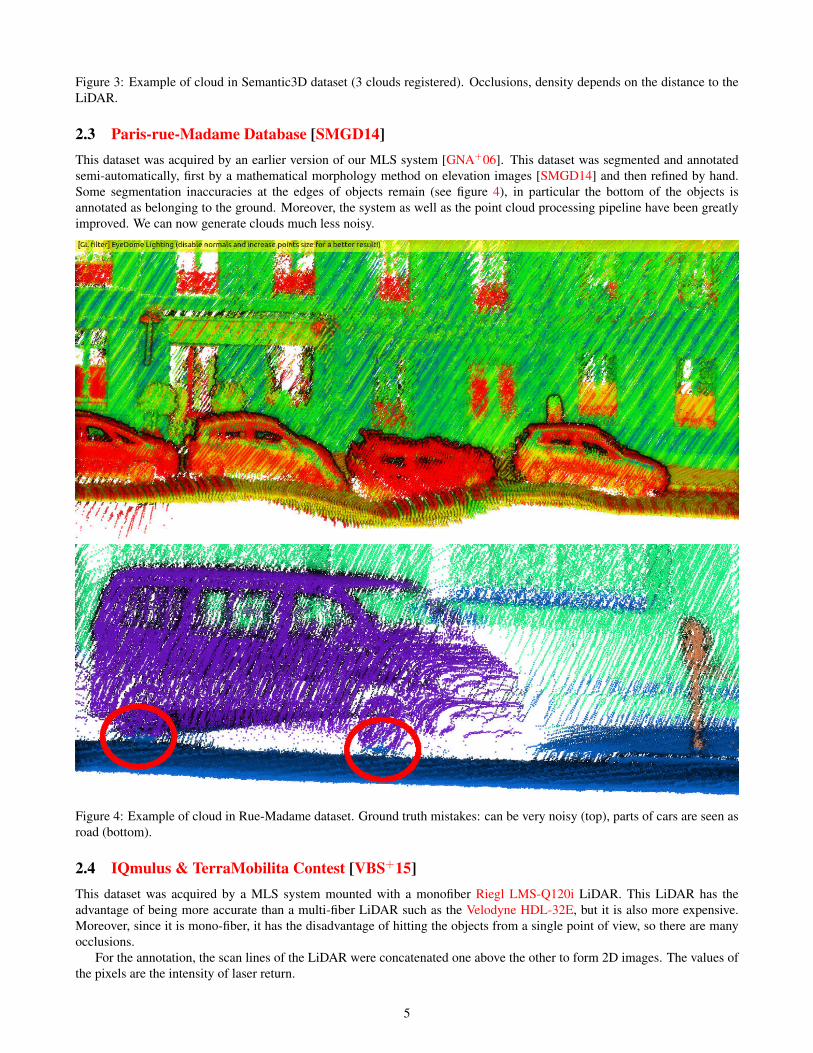
Figure 3: Example of cloud in Semantic3D dataset (3 clouds registered). Occlusions, density depends on the distance to theLiDAR.

2.3 Paris-rue-Madame Database [SMGD14]This dataset was acquired by an earlier version of our MLS system [GNA+06]. This dataset was segmented and annotatedsemi-automatically, first by a mathematical morphology method on elevation images [SMGD14] and then refined by hand.Some segmentation inaccuracies at the edges of objects remain (see figure 4), in particular the bottom of the objects isannotated as belonging to the ground. Moreover, the system as well as the point cloud processing pipeline have been greatlyimproved. We can now generate clouds much less noisy.

Figure 4: Example of cloud in Rue-Madame dataset. Ground truth mistakes: can be very noisy (top), parts of cars are seen asroad (bottom).

2.4 IQmulus & TerraMobilita Contest [VBS+15]This dataset was acquired by a MLS system mounted with a monofiber Riegl LMS-Q120i LiDAR. This LiDAR has theadvantage of being more accurate than a multi-fiber LiDAR such as the Velodyne HDL-32E, but it is also more expensive.Moreover, since it is mono-fiber, it has the disadvantage of hitting the objects from a single point of view, so there are manyocclusions.

For the annotation, the scan lines of the LiDAR were concatenated one above the other to form 2D images. The values ofthe pixels are the intensity of laser return.

5

This method has the advantage of being easy to put into production, which allowed the IGN to annotate a large dataset.However, inaccuracies in countouring annotation of 2D images generate badly classified points, the points around the occlu-sions are classified in the class of the object that creates the occlusion. (see figure 5).

Figure 5: Example of cloud in iQmulus/TerraMobilita dataset. As a monofiber LiDAR is used, there are shadows behindobjects. Moreover points of the wall behind cars are classified as car.

3 Our Dataset: Paris-Lille-3D

3.1 AcquisitionAll point clouds used in our dataset were acquired with the MLS prototype of the center for robotics of Mines ParisTech:L3D2 [GNA+06] (as seen in figure 6). It is a Citroën Jumper equipped with a GPS (Novatel FlexPak 6), an IMU (IxseaPHINS in LANDINS mode) and a Velodyne HDL-32E LiDAR mounted at the rear of the truck with an angle of 30 degreesbetween the axis of rotation and the horizontal.

6

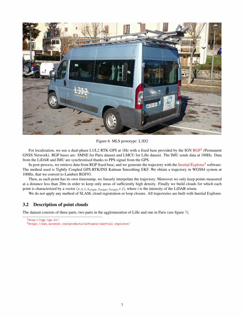
Figure 6: MLS prototype: L3D2

For localization, we use a dual-phase L1/L2 RTK-GPS at 1Hz with a fixed base provided by the IGN RGP1 (PermanentGNSS Network). RGP bases are: SMNE for Paris dataset and LMCU for Lille dataset. The IMU sends data at 100Hz. Datafrom the LiDAR and IMU are synchronised thanks to PPS signal from the GPS.

In post-process, we retrieve data from RGP fixed base, and we generate the trajectory with the Inertial Explorer2 software.The method used is Tightly Coupled GPS-RTK/INS Kalman Smoothing EKF. We obtain a trajectory in WGS84 system at100Hz, that we convert to Lambert RGF93.

Then, as each point has its own timestamp, we linearly interpolate the trajectory. Moreover we only keep points measuredat a distance less than 20m in order to keep only areas of sufficiently high density. Finally we build clouds for which eachpoint is characterized by a vector (x,y,z,xorigin,yorigin,zorigin, t, i), where i is the intensity of the LiDAR return.

We do not apply any method of SLAM, cloud registration or loop closure. All trajectories are built with Inertial Explorer.

3.2 Description of point cloudsThe dataset consists of three parts, two parts in the agglomeration of Lille and one in Paris (see figure 7).

1http://rgp.ign.fr/2https://www.novatel.com/products/software/inertial-explorer/

7

Figure 7: Trajectories of the experimental vehicle during acquisition. Top: the 2 trajectories in agglomeration of Lille are ingreen and blue. Bottom: the trajectory in Paris is in red. (Pictures from Google Maps)

For the sake of precision, an offset has been substracted in the plane (x,y) to all the points so that they hold in float (32bits). Data are distributed as explained in table 2.

Section LengthNumberof points RGF93 Offset

Lille1 1150m 71.3M (711164.0m,7064875.0m)Lille2 340m 26.8M (711164.0m,7064875.0m)Paris 450m 45.7M (650976.0m,6861466.0m)

Total 1940m 143.1M –

Table 2: Description of the three parts of the dataset.

The clouds have high density with between 1000 and 2000 points per square meter on the ground, but there are someanisotropic patterns due to the multi-beam LiDAR sensor as seen in figure 8.

8

Figure 8: Anisotropic pattern on the ground (color of points is the reflectance)

3.3 Description of segmented and classified dataThe clouds obtained were segmented and classified by hand using CloudCompare3 software. Some illustrations of the seg-mented and classified data are shown in figure 1.

We chose to re-use the class tree of iQmulus/Terramobilita benchmark, in which we only change a few classes and addclasses relevant to our dataset. It can be found at url: http://data.ign.fr/benchmarks/UrbanAnalysis/download/classes.xml For a distribution of number of points by classes, see table 3. Classes added:

� bicycle rack (id= 302021200)� statue (id= 302021300)� distribution box (id= 302040600)� lighting console (id= 302040700)� windmill (id= 302040800)

We also change the way vehicles are seen. More precisely, for each class of vehicle, we distinguish sub-classes depending onwhether they are parked, stopped (on the road) or moving. And Velib terminal is changed to bicycle terminal (id= 302021100)which is more generic.

Except the few classes mentioned above, this class tree appears to be sufficiently complete for classes encountered in ourdataset. The XML file describing this tree is named classes.xml and is provided with the dataset. We also provide threeASCII-files (.txt) containing annotations for particular samples. Each line of these files contains:

sample_id, class_id, class_name,annotation1, annotation2, ...

The most common annotations are:� "several", for example when trees are interlaced and can not be delimited precisely by hand,� "overturned", for trash cans laid on their side.

3http://www.danielgm.net/cc/

9

obje

ct

surf

ace

stat

ic

dynam

ic

nat

ura

l

Class Number of samples (of points)

Lille1 Lille2 Paris Total

unclassified 1 (54.88k) 1 (16.47k) 1 (60.79k) 3 (132.1k)other 16 (70.15k) 11 (14.10k) 11 (30.82k) 38 (115.1k)road 1 (34.80M) 1 (11.82M) 1 (19.68M) 3 (66.30M)

sidewalk 18 (8.566M) 8 (4.97M) 5 (4.6M) 31 (16.67M)island 7 (458.8k) 0 (0) 9 (82.46k) 16 (541.2k)

vegetation 32 (562.2k) 22 (512.4k) 6 (157.1k) 60 (1.232M)building 34 (18.2M) 8 (7.934M) 5 (9.431M) 47 (35.39M)post 9 (13.51k) 0 (0) 0 (0) 9 (13.51k)

bollard 122 (34.80k) 64 (7.982k) 84 (28.33k) 270 (71.10k)floor lamp 72 (232.9k) 13 (23.69k) 21 (113.2k) 106 (369.7k)traffic light 14 (25.82k) 11 (27.41k) 16 (80.76k) 41 (133.10k)traffic sign 82 (113.6k) 39 (69.89k) 17 (30.75k) 138 (214.3k)signboard 20 (68.34k) 12 (43.14k) 3 (13.41k) 35 (124.9k)mailbox 0 (0) 0 (0) 1 (4.739k) 1 (4.739k)trash can 11 (14.72k) 6 (17.43k) 22 (30.35k) 39 (62.50k)meter 0 (0) 0 (0) 2 (2.840k) 2 (2.840k)

bicycle terminal 10 (1.736k) 0 (0) 13 (6.451k) 23 (8.187k)bicycle rack 8 (774) 0 (0) 14 (8.665k) 22 (9.439k)

statue 2 (4.158k) 0 (0) 0 (0) 2 (4.158k)barrier 45 (83.94k) 5 (9.286k) 7 (56.10k) 57 (149.3k)roasting 6 (831.0k) 1 (20.82k) 4 (1.677M) 11 (2.529M)wire 34 (14.18k) 8 (9.325k) 0 (0) 42 (23.51k)

low wall 58 (840.2k) 2 (26.99k) 9 (951.4k) 69 (1.819M)shelter 0 (0) 0 (0) 3 (83.45k) 3 (83.45k)bench 5 (2.911k) 1 (364) 2 (1.391k) 8 (4.666k)

distribution box 19 (50.28k) 8 (14.89k) 3 (53.4k) 30 (118.2k)lighting console 78 (7.251k) 60 (9.731k) 9 (4.393k) 147 (21.38k)

windmill 1 (10.17k) 0 (0) 0 (0) 1 (10.17k)pedestrian 17 (24.81k) 7 (11.60k) 61 (150.2k) 85 (186.6k)

parked bicycle 15 (9.74k) 0 (0) 33 (81.67k) 48 (90.75k)mobile scooter 0 (0) 0 (0) 1 (131) 1 (131)parked scooter 0 (0) 0 (0) 31 (169.1k) 31 (169.1k)

mobile motorbike 0 (0) 0 (0) 1 (1.613k) 1 (1.613k)parked motorbike 2 (2.428k) 0 (0) 4 (14.37k) 6 (16.79k)

mobile car 21 (175.0k) 4 (40.96k) 5 (66.35k) 30 (282.3k)stopped car 0 (0) 1 (28.27k) 1 (9.375k) 2 (37.64k)parked car 182 (2.266M) 47 (853.7k) 65 (1.610M) 294 (4.730M)mobile van 3 (97.27k) 1 (41.6k) 0 (0) 4 (138.3k)parked van 5 (84.75k) 5 (85.20k) 9 (357.6k) 19 (527.6k)

stopped truck 0 (0) 0 (0) 1 (235.7k) 1 (235.7k)parked truck 2 (40.32k) 0 (0) 1 (53.44k) 3 (93.76k)stopped bus 0 (0) 0 (0) 1 (78.41k) 1 (78.41k)parked bus 1 (9.623k) 0 (0) 0 (0) 1 (9.623k)

table 0 (0) 0 (0) 2 (576) 2 (576)chair 0 (0) 0 (0) 8 (4.842k) 8 (4.842k)

trash can 138 (148.8k) 80 (115.9k) 0 (0) 218 (264.7k)waste 5 (2.307k) 0 (0) 0 (0) 5 (2.307k)natural 149 (1.233M) 47 (396.9k) 36 (1.610M) 232 (3.240M)tree 72 (2.310M) 23 (565.10k) 101 (4.755M) 196 (7.631M)

potted plant 32 (72.80k) 5 (26.96k) 0 (0) 37 (99.76k)

Total 1349 (71.36M) 501 (26.84M) 629 (45.80M) 2479 (143.10M)

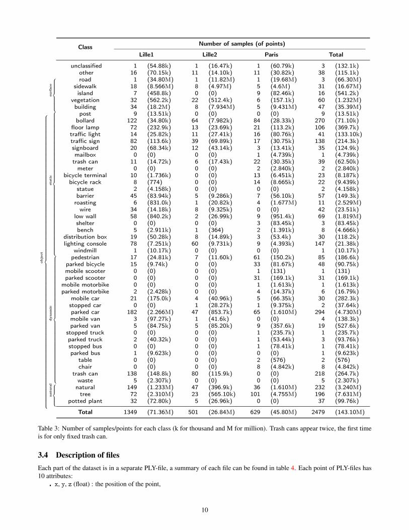
Table 3: Number of samples/points for each class (k for thousand and M for million). Trash cans appear twice, the first timeis for only fixed trash can.

3.4 Description of filesEach part of the dataset is in a separate PLY-file, a summary of each file can be found in table 4. Each point of PLY-files has10 attributes:

� x, y, z (float) : the position of the point,

10

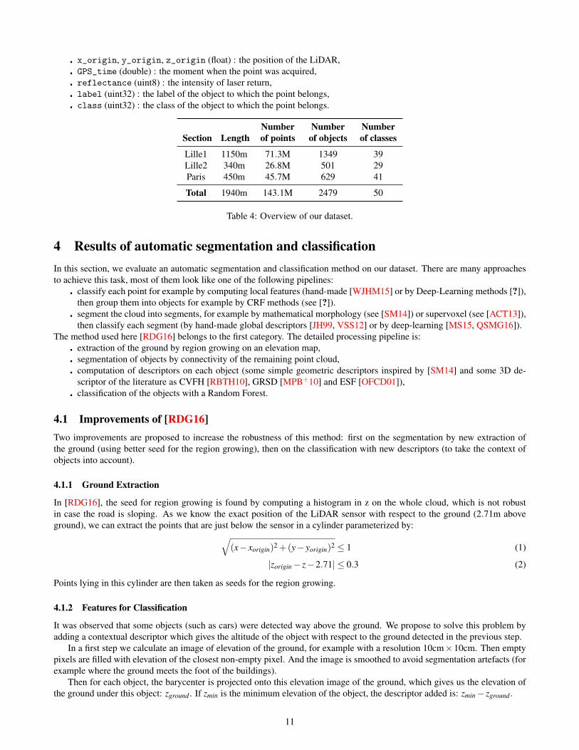
� x_origin, y_origin, z_origin (float) : the position of the LiDAR,� GPS_time (double) : the moment when the point was acquired,� reflectance (uint8) : the intensity of laser return,� label (uint32) : the label of the object to which the point belongs,� class (uint32) : the class of the object to which the point belongs.

Section LengthNumberof points

Numberof objects

Numberof classes

Lille1 1150m 71.3M 1349 39Lille2 340m 26.8M 501 29Paris 450m 45.7M 629 41

Total 1940m 143.1M 2479 50

Table 4: Overview of our dataset.

4 Results of automatic segmentation and classificationIn this section, we evaluate an automatic segmentation and classification method on our dataset. There are many approachesto achieve this task, most of them look like one of the following pipelines:

� classify each point for example by computing local features (hand-made [WJHM15] or by Deep-Learning methods [?]),then group them into objects for example by CRF methods (see [?]).

� segment the cloud into segments, for example by mathematical morphology (see [SM14]) or supervoxel (see [ACT13]),then classify each segment (by hand-made global descriptors [JH99, VSS12] or by deep-learning [MS15, QSMG16]).

The method used here [RDG16] belongs to the first category. The detailed processing pipeline is:� extraction of the ground by region growing on an elevation map,� segmentation of objects by connectivity of the remaining point cloud,� computation of descriptors on each object (some simple geometric descriptors inspired by [SM14] and some 3D de-

scriptor of the literature as CVFH [RBTH10], GRSD [MPB+10] and ESF [OFCD01]),� classification of the objects with a Random Forest.

4.1 Improvements of [RDG16]Two improvements are proposed to increase the robustness of this method: first on the segmentation by new extraction ofthe ground (using better seed for the region growing), then on the classification with new descriptors (to take the context ofobjects into account).

4.1.1 Ground Extraction

In [RDG16], the seed for region growing is found by computing a histogram in z on the whole cloud, which is not robustin case the road is sloping. As we know the exact position of the LiDAR sensor with respect to the ground (2.71m aboveground), we can extract the points that are just below the sensor in a cylinder parameterized by:

√(x− xorigin)2 +(y− yorigin)2 ≤ 1 (1)

|zorigin− z−2.71| ≤ 0.3 (2)

Points lying in this cylinder are then taken as seeds for the region growing.

4.1.2 Features for Classification

It was observed that some objects (such as cars) were detected way above the ground. We propose to solve this problem byadding a contextual descriptor which gives the altitude of the object with respect to the ground detected in the previous step.

In a first step we calculate an image of elevation of the ground, for example with a resolution 10cm×10cm. Then emptypixels are filled with elevation of the closest non-empty pixel. And the image is smoothed to avoid segmentation artefacts (forexample where the ground meets the foot of the buildings).

Then for each object, the barycenter is projected onto this elevation image of the ground, which gives us the elevation ofthe ground under this object: zground . If zmin is the minimum elevation of the object, the descriptor added is: zmin− zground .

11

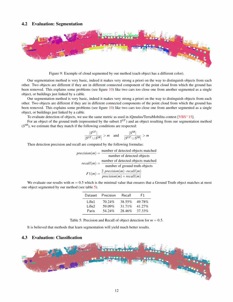
4.2 Evaluation: Segmentation

Figure 9: Exemple of cloud segmented by our method (each object has a different color).

Our segmentation method is very basic, indeed it makes very strong a priori on the way to distinguish objects from eachother. Two objects are different if they are in different connected component of the point cloud from which the ground hasbeen removed. This explains some problems (see figure 10) like two cars too close one from another segmented as a singleobject, or buildings just linked by a cable.

Our segmentation method is very basic, indeed it makes very strong a priori on the way to distinguish objects from eachother. Two objects are different if they are in different connected components of the point cloud from which the ground hasbeen removed. This explains some problems (see figure 10) like two cars too close one from another segmented as a singleobject, or buildings just linked by a cable.

To evaluate detection of objects, we use the same metric as used in iQmulus/TerraMobilita contest [VBS+15].For an object of the ground truth (represented by the subset SGT ) and an object resulting from our segmentation method

(SSR), we estimate that they match if the following conditions are respected:

|SGT ||SGT ∪SSR|

> m and|SSR|

|SGT ∪SSR|> m

Then detection precision and recall are computed by the following formulas:

precision(m) =number of detected objects matched

number of detected objects

recall(m) =number of detected objects matched

number of ground truth objects

F1(m) =2 precision(m) ·recall(m)

precision(m)+ recall(m)

We evaluate our results with m = 0.5 which is the minimal value that ensures that a Ground Truth object matches at mostone object segmented by our method (see table 5).

Dataset Precision Recall F1

Lille1 70.24% 38.55% 49.78%Lille2 59.09% 31.71% 41.27%Paris 54.24% 28.46% 37.33%

Table 5: Precision and Recall of object detection for m = 0.5.

It is believed that methods that learn segmentation will yield much better results.

4.3 Evaluation: Classification

12

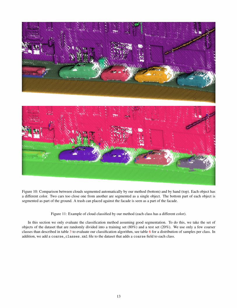
Figure 10: Comparison between clouds segmented automatically by our method (bottom) and by hand (top). Each object hasa different color. Two cars too close one from another are segmented as a single object. The bottom part of each object issegmented as part of the ground. A trash can placed against the facade is seen as a part of the facade.

Figure 11: Example of cloud classified by our method (each class has a different color).

In this section we only evaluate the classification method assuming good segmentation. To do this, we take the set ofobjects of the dataset that are randomly divided into a training set (80%) and a test set (20%). We use only a few coarserclasses than described in table 3 to evaluate our classification algorithm, see table 6 for a distribution of samples per class. Inaddition, we add a coarse_classes.xml file to the dataset that adds a coarse field to each class.

13

Class Number of samples (of points)

Lille1 Lille2 Paris Total

buildings 34 (18.2M) 8 (7.934M) 5 (9.431M) 47 (35.39M)poles 177 (385.9k) 63 (120.10k) 54 (224.7k) 294 (731.5k)

bollards 122 (34.80k) 64 (7.982k) 84 (28.33k) 270 (71.10k)trash cans 149 (163.5k) 86 (133.3k) 22 (30.35k) 257 (327.2k)barriers 109 (1.755M) 8 (57.9k) 20 (2.685M) 137 (4.497M)

pedestrians 17 (24.81k) 7 (11.60k) 61 (150.2k) 85 (186.6k)cars 211 (2.623M) 58 (1.49M) 80 (2.43M) 349 (5.715M)

natural 221 (3.543M) 70 (962.8k) 137 (6.365M) 428 (10.87M)

Total 1040 (26.55M) 364 (10.28M) 463 (20.96M) 1867 (57.79M)

Table 6: Number of samples/points for each coarse class used for classification evaluation.

Even with these coarse classes, there are a few samples in some of them. Then precision and recall numbers in table 7should be taken with caution. Metrics used to evaluate performance are the following:

P =T P

T P+FP

R =T P

T P+FN(3)

F1 =2T P

2T P+FP+FN

MCC =T P ·T N−FP ·FN√

(T P+FP)(T P+FN)(T N +FP)(T N +FN)

Where P, R, F1 and MCC represent respectively Precision, Recall, F1-score and Matthews correlation coefficient. And T P,T N, FP and FN are respectively the number of True-Positives, True-Negatives, False-Positives and False-Negatives.

Moreover, it can be noted that the best results are obtained with the combination of descriptors: Geometric and GRSD,which are the descriptors composed of the least number of variables. This can be explained by the few samples of thedataset and therefore adding a large number of features does not provide more relevant information. Then this dataset is moreappropriate for the evaluation of per-point classification methods.

Descriptors OOB Accuracy Precision Recall F1 MCC

Geom 89.22% 98.08% 89.48% 85.13% 87.23% 85.62%CVFH 70.32% 94.68% 67.23% 60.82% 63.85% 60.14%GRSD 70.02% 94.58% 64.42% 61.39% 62.82% 58.78%ESF 74.98% 95.47% 70.87% 66.99% 68.85% 65.71%

Geom+CVFH 81.94% 96.76% 79.90% 74.76% 77.21% 74.65%Geom+GRSD 89.37% 98.07% 90.33% 83.73% 86.89% 84.78%Geom+ESF 82.45% 96.81% 81.25% 77.80% 79.46% 77.30%

CVFH+GRSD 75.98% 95.67% 74.62% 68.93% 71.62% 68.33%CVFH+ESF 76.59% 95.76% 74.56% 68.81% 71.54% 68.38%GRSD+ESF 79.13% 96.19% 77.42% 73.98% 75.63% 73.02%

Geom+CVFH+GRSD 83.00% 96.98% 81.54% 76.03% 78.64% 76.10%Geom+CVFH+ESF 82.23% 96.76% 81.75% 76.89% 79.22% 76.88%Geom+GRSD+ESF 83.90% 97.05% 82.26% 79.65% 80.91% 78.90%CVFH+GRSD+ESF 79.25% 96.27% 79.04% 74.04% 76.43% 73.75%

Geom+CVFH+GRSD+ESF 83.41% 97.00% 82.91% 79.07% 80.92% 78.78%

Table 7: Classification performance for each combination of descriptors, these metrics are averaged over all classes (the OOBscore is given by Random-Forest during training).

It can be concluded that it is not necessary to calculate all the descriptors to obtain the best classification results. It ispossible to gain in computation time by calculating only the geometric descriptors and GRSD (see table 8 for precise gains).

14

And for applications where time is critical, we can even calculate only the geometric descriptors (which also avoids having tocalculate the normals).

Descriptors Proportion Mean Time per object (ms)

Geom 3.22% 0.9

CVFH 44.92% 11.9

GRSD 12.04% 3.2

ESF 39.82% 10.6

Total 100% 26.6

Normals 47.9

Table 8: Mean computational time for calculating descriptors on segmented objects. Time to compute normal vectors is addedfor comparison.

5 ConclusionWe presented a dataset of urban 3D point cloud for automatic segmentation and classification. This dataset contains 140million points on 2km in two different cities. The objects were segmented by hand and a class was associated with each oneamong 50 classes.

We hope that this dataset will help to train and evaluate methods as deep-learning, which are very demanding in terms ofquantity of points.

In addition, we have tested a first method of segmentation and automatic classification from [RDG16] to which we havemade some improvements for robustness.

References[ACT13] Ahmad Kamal Aijazi, Paul Checchin, and Laurent Trassoudaine. Segmentation based classification of 3d

urban point clouds: A super-voxel based approach with evaluation. Remote Sensing, 5(4):1624–1650, 2013.

[AEHKL+16] Sami Abu-El-Haija, Nisarg Kothari, Joonseok Lee, Paul Natsev, George Toderici, Balakrishnan Varadarajan,and Sudheendra Vijayanarasimhan. Youtube-8m: A large-scale video classification benchmark. arXiv preprintarXiv:1609.08675, 2016.

[CBUE16] Nicholas Carlevaris-Bianco, Arash K Ushani, and Ryan M Eustice. University of michigan north campuslong-term vision and lidar dataset. The International Journal of Robotics Research, 35(9):1023–1035, 2016.

[COR+16] Marius Cordts, Mohamed Omran, Sebastian Ramos, Timo Rehfeld, Markus Enzweiler, Rodrigo Benenson,Uwe Franke, Stefan Roth, and Bernt Schiele. The cityscapes dataset for semantic urban scene understanding.In Proceedings of the IEEE Conference on Computer Vision and Pattern Recognition, pages 3213–3223, 2016.

[DDS+09] Jia Deng, Wei Dong, Richard Socher, Li-Jia Li, Kai Li, and Li Fei-Fei. Imagenet: A large-scale hierarchicalimage database. In Computer Vision and Pattern Recognition, 2009. CVPR 2009. IEEE Conference on, pages248–255. IEEE, 2009.

[FMH+15] Francis Ferraro, Nasrin Mostafazadeh, Ting-Hao Huang, Lucy Vanderwende, Jacob Devlin, Michel Gal-ley, and Margaret Mitchell. A survey of current datasets for vision and language research. arXiv preprintarXiv:1506.06833, 2015.

[GLU12] Andreas Geiger, Philip Lenz, and Raquel Urtasun. Are we ready for autonomous driving? the kitti visionbenchmark suite. In Conference on Computer Vision and Pattern Recognition (CVPR), 2012.

[GNA+06] F Goulette, F Nashashibi, I Abuhadrous, S Ammoun, and C Laurgeau. An integrated on-board laser rangesensing system for on-the-way city and road modelling. The International Archives of the Photogrammetry,Remote Sensing and Spatial Information Sciences, 34(Part A), 2006.

15

[HWS16] Timo Hackel, Jan D Wegner, and Konrad Schindler. Fast semantic segmentation of 3d point clouds withstrongly varying density. ISPRS Annals of the Photogrammetry, Remote Sensing and Spatial InformationSciences, Prague, Czech Republic, 3:177–184, 2016.

[JH99] Andrew E Johnson and Martial Hebert. Using spin images for efficient object recognition in cluttered 3dscenes. Pattern Analysis and Machine Intelligence, IEEE Transactions on, 21(5):433–449, 1999.

[LMB+14] Tsung-Yi Lin, Michael Maire, Serge Belongie, James Hays, Pietro Perona, Deva Ramanan, Piotr Dollár, andC Lawrence Zitnick. Microsoft coco: Common objects in context. In European Conference on ComputerVision, pages 740–755. Springer, 2014.

[MBVH09] Delfina Munoz, J Andrew Bagnell, Nicolas Vandapel, and Martial Hebert. Contextual classification withfunctional max-margin markov networks. In Computer Vision and Pattern Recognition, 2009. CVPR 2009.IEEE Conference on, pages 975–982. IEEE, 2009.

[MPB+10] Zoltan-Csaba Marton, Dejan Pangercic, Nico Blodow, Jonathan Kleinehellefort, and Michael Beetz. General3d modelling of novel objects from a single view. In Intelligent Robots and Systems (IROS), 2010 IEEE/RSJInternational Conference on, pages 3700–3705. IEEE, 2010.

[MPLN17] Will Maddern, Geoff Pascoe, Chris Linegar, and Paul Newman. 1 Year, 1000km: The Oxford RobotCarDataset. The International Journal of Robotics Research (IJRR), 36(1):3–15, 2017.

[MS15] Daniel Maturana and Sebastian Scherer. Voxnet: A 3d convolutional neural network for real-time objectrecognition. In Intelligent Robots and Systems (IROS), 2015 IEEE/RSJ International Conference on, pages922–928. IEEE, 2015.

[NRS14] Joachim Niemeyer, Franz Rottensteiner, and Uwe Soergel. Contextual classification of lidar data and buildingobject detection in urban areas. ISPRS journal of photogrammetry and remote sensing, 87:152–165, 2014.

[OFCD01] Robert Osada, Thomas Funkhouser, Bernard Chazelle, and David Dobkin. Matching 3d models with shapedistributions. In Shape Modeling and Applications, SMI 2001 International Conference on., pages 154–166.IEEE, 2001.

[PME11] Gaurav Pandey, James R McBride, and Ryan M Eustice. Ford campus vision and lidar data set. The Interna-tional Journal of Robotics Research, 30(13):1543–1552, 2011.

[QSMG16] Charles R Qi, Hao Su, Kaichun Mo, and Leonidas J Guibas. Pointnet: Deep learning on point sets for 3dclassification and segmentation. arXiv preprint arXiv:1612.00593, 2016.

[RBTH10] Radu Bogdan Rusu, Gary Bradski, Romain Thibaux, and John Hsu. Fast 3d recognition and pose usingthe viewpoint feature histogram. In Intelligent Robots and Systems (IROS), 2010 IEEE/RSJ InternationalConference on, pages 2155–2162. IEEE, 2010.

[RDG16] Xavier Roynard, Jean-Emmanuel Deschaud, and Francois Goulette. Fast and robust segmentation and classi-fication for change detection in urban point clouds. In ISPRS 2016-XXIII ISPRS Congress, 2016.

[SHK+14] Daniel Scharstein, Heiko Hirschmüller, York Kitajima, Greg Krathwohl, Nera Nešic, Xi Wang, and PorterWestling. High-resolution stereo datasets with subpixel-accurate ground truth. In German Conference onPattern Recognition, pages 31–42. Springer, 2014.

[SM14] Andrés Serna and Beatriz Marcotegui. Detection, segmentation and classification of 3d urban objects usingmathematical morphology and supervised learning. ISPRS Journal of Photogrammetry and Remote Sensing,93:243–255, 2014.

[SMGD14] Andrés Serna, Beatriz Marcotegui, François Goulette, and Jean-Emmanuel Deschaud. Paris-rue-madamedatabase: a 3d mobile laser scanner dataset for benchmarking urban detection, segmentation and classifi-cation methods. In 4th International Conference on Pattern Recognition, Applications and Methods ICPRAM2014, 2014.

[VBS+15] Bruno Vallet, Mathieu Brédif, Andrés Serna, Beatriz Marcotegui, and Nicolas Paparoditis. Terramo-bilita/iqmulus urban point cloud analysis benchmark. Computers & Graphics, 49:126–133, 2015.

16

[VSS12] Alexander Velizhev, Roman Shapovalov, and Konrad Schindler. Implicit shape models for object detection in3d point clouds. In International Society of Photogrammetry and Remote Sensing Congress, volume 2, 2012.

[WJHM15] Martin Weinmann, Boris Jutzi, Stefan Hinz, and Clément Mallet. Semantic point cloud interpretation basedon optimal neighborhoods, relevant features and efficient classifiers. ISPRS Journal of Photogrammetry andRemote Sensing, 105:286–304, 2015.

17