Embed Size (px)
Citation preview

Hitotsubashi University Repository
Title Pareto Distributions in Economic Growth Models
Author(s) Nirei, Makoto
Citation
Issue Date 2009-07
Type Technical Report
Text Version publisher
URL http://hdl.handle.net/10086/17503
Right

HitotsubashiU
niversityInstitute of Innovation R
esearch
Institute of Innovation ResearchHitotsubashi University
Tokyo, Japanhttp://www.iir.hit-u.ac.jp

Pareto Distributions in Economic Growth Models
Makoto Nirei∗
Institute of Innovation Research, Hitotsubashi University
July 22, 2009
Abstract
This paper analytically demonstrates that the tails of income and wealth distributions
converge to a Pareto distribution in a variation of the Solow or Ramsey growth model
where households bear idiosyncratic investment shocks. The Pareto exponent is shown
to be decreasing in the shock variance, increasing in the growth rate, and increased by
redistribution policies by income or bequest tax. Simulations show that even in the short
run the exponent is affected by those fundamentals. We argue that the Pareto exponent
is determined by the balance between the savings from labor income and the asset income
contributed by risk-taking behavior.
1 Introduction
It is well known that the tail distributions of income and wealth follow a Pareto distri-
bution in which the frequency decays in power as Pr(x) ∝ x−λ−1. Researchers widely
hold the view that the Pareto distribution is generated by multiplicative shocks in the
∗Address: 2-1 Naka, Kunitachi, Tokyo 186-8603, Japan. Phone: +81 (42) 580-8417. Fax: +81 (42)
580-8410. E-mail: [email protected]. I am grateful to Yoshi Fujiwara and Hideaki Aoyama for generously
sharing data. I have benefited by comments from Xavier Gabaix and Wataru Souma. I wish to thank Professor
Tsuneo Ishikawa for introducing me to this research field.
1

104
105
106
107
10−4
10−3
10−2
10−1
Income (2005 dollars)
Cum
ulat
ive
dist
ribut
ion
1917192919451973198519912005
Figure 1: Income distributions above the top ten percentile
wealth accumulation process. In this paper, we formalize this idea in the framework of
the standard models of economic growth.
There are renewed interests in the tail distributions of income and wealth. Recent
studies by Feenberg and Poterba [9] and Piketty and Saez [24] investigated the time series
of top income share in the U.S. by using tax returns data. Figure 1 shows the income
distribution tails from 1917 to 2006 in the data compiled by Piketty and Saez [24]. The
distribution is plotted in log-log scale and cumulated from above to the 90th percentile.
We note that a linear line fits the tail distributions well in the log-log scale. This implies
that the tail part follows log Pr(X > x) = a− λ log x, which is called Pareto distribution
and its slope λ is called Pareto exponent. The tail distribution is more egalitarian when
λ is larger and thus when the slope is steeper. The good fit of the Pareto distribution in
the tail is more evident in Figure 2, which plots the income distributions in Japan based
on the tax returns data as in Souma [30], Fujiwara et al.[11], and Moriguchi and Saez
[20]. The long tail covers more than a factor of twenty in relative income and displays
a clear Paretian tail regardless of the economic situations Japan underwent, the bubble
era or the lost decade.
2

10−1 100 101 102 10310−8
10−6
10−4
10−2
100
Income normalized by average
Cum
ulat
ive
prob
abilit
y
1961−19801981−19901991−1999
Figure 2: Income distributions in Japan (Source: Fujiwara et al. [11], Nirei and Souma [22].)
Figure 3 plots the time series of the U.S. Pareto exponent λ estimated for the various
ranges of the tail.1 We observe a slow movement of λ decade by decade: the U.S. Pareto
exponent has increased steadily until 1960s, and since then declined fairly monotonically.
The Pareto exponent stays in the range 1.5 to 3. But there is no clear time-trend for
equalization or inequalization. In fact, we observe that the distributions in 1917 and 2006
are nearly parallel in Figure 1. This means that the income at each percentile grew at
the same average rate in the long run. The Pareto exponent in Japan also stays around
2 as shown in Figure 2.
The stationarity of the Pareto exponent implies that the income distribution is char-
acterized as a stationary distribution when normalized by the average income each year,
since the Pareto distribution is “scale-free” (i.e., invariant in the change of units). This
1We estimate λ by a linear fit on the log-log plot. The linear fit is often problematic for estimating the tail
exponent, because there are few observations on the tail for sampled data. This sampling error is not a big
problem for our binned data, however, because each bin includes all the population within the bracket and
thus contains a large number of observations.
3

1920 1940 1960 1980 2000
1.5
2
2.5
3
Year
Par
eto
expo
nent
P99−P99.9P99−P99.99P99.5−P99.9P99.5−P99.99
Figure 3: Pareto exponents for the U.S. income distributions
contrasts with the log-normal hypothesis of income distribution. If income incurs a mul-
tiplicative shock that is independent of income level (“Gibrat’s law”), then the income
follows a log-normal distribution. On the one hand, a log-normal distribution approxi-
mates a power-law distribution in an upper-middle range well (Montroll and Shlesinger
[19]). On the other hand, the cross-sectional variance of log-income must increase linearly
over time in the log-normal development of the distribution, and hence the dispersion of
relative income diverges over time. Also, the log-normal development implies that the
Pareto exponent becomes smaller and smaller as time passes. To the contrary, our plot
exhibits no such trend in the Pareto exponent, and the variance of log-income is stationary
over time as noted by Kalecki [14]. Thus, Gibrat’s hypothesis of log-normal development
need be modified.
We can obtain a stationary Pareto exponent by slightly modifying the multiplica-
tive process in such a way that there is a small dragging force that prevents the very
top portion of the distribution diverging. This was the idea of Champernowne [7], and
subsequently a number of stochastic process models are proposed such as the preferen-
tial attachment and birth-and-death process (Simon [29], Rutherford [25], Sargan [27],
4
Shorrocks [28]), and stochastic savings (Vaughan [32]). Models of randomly divided in-
heritance, along the line of Wold and Whittle [33], make a natural economic sense of the
dragging force for the stationarity, as later pursued by Blinder [4] and Dutta and Michel
[8]. Pestieau and Possen [23] presented a model of rational bequests with random returns
to asset, in which the wealth distribution follows log-normal development. They showed
that the variance of log-wealth can be bounded if their model incorporates a convex estate
tax.
Another mechanism for the bounded log-variance is a reflexive lower bound, which
pushes up the bottom of the distribution faster than the drift growth (total growth less
diffusion effects) of the rest and thus achieves the stationary relative distribution. The
analysis is based on the work of Kesten [15] and used by Levy and Solomon [16] and
Gabaix [12]. The present paper extends this line of research by articulating the economic
meanings of the multiplicative shocks and the reflexive lower bound in the context of
the standard growth model. While we mainly focus on the reflexive lower bound, we
also incorporate the effect of random inheritances in the Ramsey model by utilizing the
multiplicative process with reset events studied by Manrubia and Zanette [17].
In the growth literature, there are relatively few studies on the shape of cross-section
distribution of income and wealth, compared to the literature on the relation between
inequality and growth. Perhaps the most celebrated is Stiglitz [31] which highlights the
equalizing force of the Solow model. Numerical studies by Huggett [13] and Castaneda,
Dıaz-Gimenez, and Rıos-Rull [6] successfully capture the overall shape of earnings and
wealth distributions in a modern dynamic general equilibrium model. The present pa-
per complements theirs by concentrating on the analytical characterization of the tail
distribution, which covers a small fraction of population but carries a big impact on the
inequality measures because of its large shares in income and wealth.
In this paper, we develop a simple theory of income distribution in the Solow and
Ramsey growth models. We incorporate an idiosyncratic asset return shock, and show
that the Solow model generates a stationary Pareto distribution for the detrended house-
hold income at the balanced growth path. Pareto exponent λ is analytically determined
by fundamental parameters. The determinant of λ is summarized by the balance between
5

the inflow from the middle class into the tail part and the inequalization force within the
tail part. The inflow is represented by the savings from wage income that pushes up the
bottom of the wealth distribution. The inequalization force is captured by the capital
income that is attributed to risk taking behaviors of the top income earners. When the
two variables are equal, Pareto exponent is determined at the historically stationary level,
λ = 2.
We establish some comparative statics for the Pareto exponent analytically. The
Pareto exponent is decreasing in the returns shock variance, and increasing in the tech-
nological growth rate. This is interpreted by the balance between the middle-class savings
and the diffusion: the shock variance increases the diffusion, while the growth contributes
to the savings size. The savings rate per se turns out to be neutral on the determination
of the Pareto exponent, because it affects the savings amount and the variance of the as-
set growth equally. However, a heterogeneous change in savings behavior does affect the
Pareto exponent. For example, a lowered savings rate in the low asset group reduces the
savings amount and thus decreases the Pareto exponent. Redistribution policies financed
by flat-rate taxes on income and bequest are shown to raise the Pareto exponent. Finally,
a decline in mortality rate lowers the Pareto exponent.
The rest of the paper is organized as follows. In Section 2, the Solow model with
uninsurable investment risk is presented and the main result is shown. In Section 3, the
Solow model is extended to incorporate redistribution policies by income or bequest tax,
and the sensitivity of the exponent is investigated. In Section 4, the stationary Pareto
distribution is derived in the Ramsey model with random discontinuation of household
lineage. Section 5 concludes.
2 Solow model
In this section, we present a Solow growth model with an uninsurable and undiversifiable
investment risk. Consider a continuum of infinitely-living consumers i ∈ [0, 1]. Each
consumer is endowed with one unit of labor, an initial capital ki,0, and a “backyard”
6

production technology that is specified by a Cobb-Douglas production function:
yi,t = kαi,t(ai,tli,t)1−α (1)
where li,t is the labor employed by i and ki,t is the capital owned by i. The labor-
augmenting productivity ai,t is an i.i.d. random variable across households and across
periods with a common trend γ > 1:
ai,t = γtεi,t (2)
where εi,t is a temporary productivity shock with mean 1. Households do not have a
means to insure against the productivity shock εi,t except for its own savings. Note that
the effect of the shock is temporary. Even if i drew a bad shock in t − 1, its average
productivity is flushed to the trend level γt in the next period.
Each household supplies one unit of labor inelastically. The capital accumulation
follows:
ki,t+1 = (1− δ)ki,t + s(πi,t + wt) (3)
where s is a constant savings rate and πi,t +wt is the income of household i. πi,t denotes
the profit from the production:
πi,t = maxli,t,yi,t
yi,t − wtli,t (4)
subject to the production function (1). The first order condition of the profit maximiza-
tion yields a labor demand function:
li,t = (1− α)1/αa(1−α)/αi,t w
−1/αt ki,t. (5)
Plugging into the production function, we obtain a supply function:
yi,t = (1− α)1/α−1a(1−α)/αi,t w
1−1/αt ki,t. (6)
By combining (4,5,6), we obtain that πi,t = αyi,t and wtli,t = (1− α)yi,t.
The aggregate labor supply is 1, and thus the labor market clearing implies∫ 1
0li,tdi =
1. Define the aggregate output and capital as Yt ≡∫ 1
0yi,tdi and Kt ≡
∫ 1
0ki,tdi. Then we
obtain the labor share of income to be a constant 1− α:
wt = (1− α)Yt. (7)
7

Plugging into (6) and integrating, we obtain an aggregate relation:
Yt = E(a(1−α)/αi,t )αKα
t = E(ε(1−α)/αi,t )αγt(1−α)Kα
t . (8)
By aggregating the capital accumulation equations (3) across households, we repro-
duce the equation of motion for the aggregate capital in the Solow model:
Kt+1 = (1− δ)Kt + sYt. (9)
Define a detrended aggregate capital as:
Xt ≡Kt
γt. (10)
Then the equation of motion is written as:
γXt+1 = (1− δ)Xt + sηXαt (11)
where
η ≡ E(ε(1−α)/αi,t
)α. (12)
Equation (11) shows the deterministic dynamics of Xt, and its steady state is solved as:
X =(
sη
γ − 1 + δ
)1/(1−α)
. (13)
Since α < 1, the steady state is stable and unique in the domain X > 0. The model
preserves the standard implications of the Solow model on the aggregate characteristics
of the balanced growth path. The actual investment equals the break-even investment
on the balanced growth path as s(Yt/γt) = (γ − 1 + δ)X. The long-run output-capital
ratio ( ¯Y/K) is equal to (γ − 1 + δ)/s. The golden-rule savings rate is equal to α under
the Cobb-Douglas technology.
We now turn to the dynamics of individual capital. Define a detrended individual
capital:
xi,t ≡ki,tγt. (14)
Substituting in (3), we obtain:
γxi,t+1 =(
1− δ + sαXα−1t (εt/η)(1−α)/α
)xi,t + sη(1− α)Xα
t . (15)
8

The system of equations (11,15) defines the dynamics of (xi,t, Xt). We saw that Xt
deterministically converges to the steady state X. At the steady state, the dynamics of
an individual capital xi,t (15) becomes:
xi,t+1 = gi,txi,t + z (16)
where
gi,t ≡1− δγ
+α(γ − 1 + δ)
γ
ε(1−α)/αi,t
E(ε(1−α)/αi,t )
(17)
z ≡ sη(1− α)γ
Xα =sη(1− α)
γ
(sη
γ − 1 + δ
)α/(1−α)
. (18)
gi,t is the return to detrended capital (1 − δ + sπi,t/xi,t)/γ, and z is the savings from
detrended labor income swt/γt+1. Equation (16) is called a Kesten process, which is a
stochastic process with a multiplicative shock and an additive shock (a constant in our
case). At the steady state,
E(gi,t) = 1− z/x (19)
must hold, where the steady state x is equal to the aggregate steady state X. E(gi,t) =
α+ (1−α)(1− δ)/γ < 1 holds by the definition of gi,t (17), and hence the Kesten process
is stationary. The following proposition is obtained by applying the theorem shown by
Kesten [15] (see also [16] and [12]):
Proposition 1 Household’s detrended capital xi,t has a stationary distribution whose
tail follows a Pareto distribution:
Pr(xi,t > x) ∝ x−λ (20)
where the Pareto exponent λ is determined by the condition:
E(gλi,t) = 1. (21)
Household’s income πi,t + wt also follows the same tail distribution.
The condition (21) is understood as follows (see Gabaix [12]). When xt has a power-
law tail Pr(xt > x) = c0x−λ for a large x, the cumulative probability of xt+1 satisfies
9

Pr(xt+1 > x) = Pr(xt > (x− z)/gt) = c0(x− z)−λ∫gλt F (dgt) for a large x and a fixed z,
where F denotes the distribution function of gt. Thus, xt+1 has the same distribution as
xt in the tail only if E(gλt ) = 1. Household’s income also follows the same distribution,
because the capital income πi,t is proportional to ki,t and the labor income wt is constant
across households and much smaller than the capital income in the tail part.
In what follows we assume that the returns shock log εi,t follows a normal distribution
with mean −σ2/2 and variance σ2. We first establish that λ > 1 and that λ is decreasing
in the shock variance.
Proposition 2 There exists σ such that for σ > σ Equation (21) determines the Pareto
exponent λ uniquely. The Pareto exponent always satisfies λ > 1 and the stationary
distribution has a finite mean. Moreover, λ is decreasing in σ.
Proof is deferred to Appendix A.
Proposition 2 conducts a comparative static of λ with respect to σ. To do so, we need
to show that E(gλi,t) is strictly increasing in λ. Showing this is easy if δ = 1, since then
gi,t follows a two-parameter log-normal distribution. Under the 100% depreciation, we
obtain the analytic solution for λ as follows (see Appendix B for the derivation):
λ|δ=1 = 1 +(
α
1− α
)2 log(1/α)σ2/2
. (22)
This expression captures our result that λ is greater than 1 and decreasing in σ. Propo-
sition 2 establishes this property in a more realistic case of partial depreciation under
which gi,t follows a shifted log-normal distribution. The property is shown for a suffi-
ciently large variance σ2. This is required so that g > 1 occurs with a sufficiently large
probability. The lower bound σ takes the value about 1.8 under the benchmark param-
eter set (α = 1/3, δ = 0.1, γ = 1.03). This is a sufficient condition, however, and the
condition can be relaxed. In simulations we use the value σ2 = 1.1 and above, and we
observe that E(gλi,t) is still increasing in λ.
The Pareto distribution has a finite mean only if λ > 1 and a finite variance only
if λ > 2. Since E(gi,t) < 1, it immediately follows that λ > 1 and that the stationary
distribution of xi,t has a finite mean in our model. When λ is found in the range between
1 and 2, the capital distribution has a finite mean but an infinite variance. The infinite
10

variance implies that, in an economy with finite households, the population variance grows
unboundedly as the population size increases.
Proposition 2 shows that the idiosyncratic investment shocks generate a “top heavy”
distribution, and at the same time it shows that there is a certain limit in the wealth
inequality generated by the Solow economy, since the stationary Pareto exponent cannot
be smaller than 1. Pareto distribution is “top heavy” in the sense that a sizable fraction
of total wealth is possessed by the richest few. The richest P fraction of population owns
P 1−1/λ fraction of total wealth when λ > 1 (Newman [21]). For λ = 2, this implies that
the top 1 percent owns 10% of total wealth. If λ < 1, the wealth share possessed by the
rich converges to 1 as the population grows to infinity. Namely, virtually all of the wealth
belongs to the richest few. Also when λ < 1, the expected ratio of the single richest
person’s wealth to the economy’s total wealth converges to 1 − λ (Feller [10]). Such an
economy almost resembles an aristocracy where a single person owns a fraction of total
wealth. Proposition 2 shows that the Solow economy does not allow such an extreme
concentration of wealth, because λ cannot be smaller than 1 at the stationary state.
Empirical income distributions show that the Pareto exponent transits below and
above 2, in the range between 1.5 and 3. This implies that the economy goes back
and forth between the two regimes, one with finite variance of income (λ > 2) and one
with infinite variance (λ ≤ 2). The two regimes differ not only quantitatively but also
qualitatively, since for λ < 2 almost all of the sum of the variances of idiosyncratic risks is
born by the wealthiest few whereas the risks are more evenly distributed for λ > 2. This
is seen as follows. In our economy, the households do not diversify investment risks. Thus
the variance of their income increases proportionally to their wealth x2i,t, which follows
a Paretian tail with exponent λ/2. Thus, the income variance is distributed as a Pareto
distribution with exponent less than 1, which is so unequal that the single wealthiest
household bears a fraction 1 − λ/2 of the sum of the variances of the idiosyncratic risks
across households, and virtually all of the sum of the variances are born by the richest few
percentile. Thus, in the Solow model, the concentration of the wealth can be interpreted
as the result of the extraordinary concentration of risk bearings.
We can obtain an intuitive characterization for the threshold point λ = 2 for the two
11

regimes under the assumption that log εi,t follows a normal distribution with mean −σ2/2
and variance σ2 as follows.
Proposition 3 The Pareto exponent λ is greater than (less than) 2 when σ < σ (> σ)
where:
σ2 =(
α
1− α
)2
log(
1α2
(1− 2α
γ/(1− δ)− 1
)). (23)
Moreover, λ is increasing in γ and in δ in the neighborhood of λ = 2.
Proof is deferred to Appendix C.
Proposition 3 relates the Pareto exponent with the variance of the productivity shock,
the growth rate, and the depreciation rate. The Pareto exponent is smaller when the
variance is larger. At the variance σ2, the income distribution lays at the boarder between
the two regimes where the variance of cross-sectional income is well defined and where
the variance diverges. We also note that γ and δ both affect positively to λ around λ = 2.
That is, a faster growth or a faster wealth depreciation helps equalization in the tail.
A faster economic growth helps equalization, because the importance of the risk-taking
behaviors (σ2) is reduced relative to the drift growth. In other words, a faster trend
growth increases the inflow from the middle class to the rich while the diffusion among
the rich is unchanged. We explore this intuition further in the following.
The threshold variance is alternatively shown as follows. At λ = 2, E(g2i,t) = 1
must hold by (21). Using E(gi,t) = 1 − z/x, this leads to the condition Var(gi,t)/2 =
z/x− (z/x)2/2. The key variable z/x is equivalently expressed as:
z
x=s(1− α)
γ
¯(Y
K
)=
(1− α)(γ − 1 + δ)γ
. (24)
Under the benchmark parameters α = 1/3, δ = 0.1, and γ = 1.03, we obtain z/x to
be around 0.08. We can thus neglect the second order term (z/x)2 and obtain z ≈
xVar(gi,t)/2 as the condition for λ = 2. The right hand side expresses the growth of
capital due to the diffusion effect. As we argue later, we may interpret this term as
the capital income due to the risk taking behavior. The left hand side z represents the
savings from the labor income. Then, the Pareto exponent is determined at 2 when
the contribution of labor to capital accumulation balances with the contribution of risk
12

taking. In other words, the stationary distribution of income exhibits a finite or infinite
variance depending on whether the wage contribution to capital accumulation exceeds or
falls short of the contribution from risk takings.
When ε follows a log-normal distribution, g is approximated in the first order by a
log-normal distribution around the mean of ε. We explore the formula for λ under the
first-order approximation. By the condition (21), we obtain:
λ ≈ − E(log g)Var(log g)/2
. (25)
Note that for a log-normal g we have:
log E(g) = E(log g) + Var(log g)/2. (26)
Thus, (25) indicates that λ is determined by the relative importance of the drift and the
diffusion of the capital growth rates both of which contribute to the overall growth rate.
Using the condition E(g) = 1− z/x, we obtain an alternative expression:
λ ≈ 1 +− log(1− z/x)Var(log g)/2
(27)
as in Gabaix [12]. We observe that the Pareto exponent λ is always greater than 1, and
it declines to 1 as the savings z decreases to 0 or the diffusion effect Var(log g) increases
to infinity. For a small z/x, the expression is further approximated as:
λ ≈ 1 +z
xVar(log g)/2. (28)
Var(log g)/2 is the contribution of the diffusion to the total return of asset. Thus, the
Pareto exponent is equal to 2 when the savings z is equal to the part of capital income
contributed by the risk-taking behavior.
The intuition of our mechanism to generate Pareto distribution is following. The
multiplicative process is one of the most natural mechanisms for the right-skewed, heavy
tailed distribution of income and wealth as the extensive literature on the Pareto distribu-
tion indicates. Without some modification, however, the multiplicative process leads to
a log-normal development and does not generate the Pareto distribution nor the station-
ary variance of log income. Incorporating the wage income in the accumulation process
13
just does this modification. In our model, the savings from wage income (z) serves as
a reflexive lower bound of the multiplicative wealth accumulation. Moreover, we find
that the Pareto exponent is determined by the balance between the contributions of this
additive term (savings) and the diffusion term (capital income). The savings from the
wage income determines the mobility between the tail wealth group and the rest. Thus,
we can interpret our result as the mobility between the top and the middle sections of
income determines the Pareto exponent.
The close connection between the multiplicative process and the Pareto distribution
may be illustrated as follows. Pareto distribution implies a self-similar structure of the
distribution in terms of the change of units. Suppose that you belong to a “millionaire
club” where all the members earn more than a million. In the club, you find that 10−λ
of the club members earn 10 times more than you. If λ = 2, this is one percent of the all
members. Suppose that, after some hard work, you now belong to a ten-million earners’
club. But then, you find again that one percent of the club members earn 10 times more
than you do. If your preference for wealth is ordered by the relative position of your
wealth among your social peers, you will never be satisfied by climbing up the social
ladder of millionaire clubs. This observation is in good contrast with the “memoryless”
property of an exponential distribution in addition. An exponential distribution charac-
terizes the middle-class distribution well. In any of the social clubs within the region of
the exponential distribution, you will find the same fraction of club members who earn
$10000 more than you. The contrast between the Pareto distribution and the exponential
distribution corresponds to that the Pareto distribution is generated by a multiplicative
process with lower bound while the exponential distribution is generated by an additive
process with lower bound [16]. Under this perspective, Nirei and Souma [22] showed that
the middle-class distribution as well as the tail distribution can be reproduced in a simple
growth model with multiplicative returns shocks and additive wage shocks.
14

3 Sensitivity Analysis
3.1 Redistribution
In this section, we extend the Solow framework to redistribution policies financed by
taxes on income and bequest. Tax proceeds are redistributed to households equally. Let
τy denote the flat-rate tax on income, and let τb denote the flat-rate bequest tax on
inherited wealth. We assume that a household changes generations with probability µ
in each period. Thus, the household’s wealth is taxed at flat rate τb with probability
µ and remains intact with probability 1 − µ. Denote the bequest event by a random
variable 1b that takes 1 with probability µ and 0 with probability 1 − µ. Then, the
capital accumulation equation (3) is modified as follows:
ki,t+1 = (1− δ − 1bτb)ki,t + s((1− τy)(πi,t + wt) + τyYt + τbµKt). (29)
By aggregating, we recover the law of motion for Xt as in (11). Therefore, the redistri-
bution policy does not affect X or aggregate output at the steady state. Combining with
(29), the accumulation equation for an individual wealth is rewritten at X as follows:
xi,t+1 = gi,txi,t + z (30)
where the newly defined growth rate gi,t and the savings term z are:
gi,t ≡1− δ − 1bτb
γ+
(1− τy)α(γ − 1 + δ)γ
ε(1−α)/αi,t
E(ε(1−α)/αi,t )
(31)
z ≡ sη(1− α+ ατy)γ
(sη
γ − 1 + δ
)α/(1−α)
+ τbµ
(sη
γ − 1 + δ
)1/(1−α)
. (32)
This is a Kesten process, and the Pareto distribution immediately obtains.
Proposition 4 Under the redistribution policy, a household’s wealth xi,t has a stationary
distribution whose tail follows a Pareto distribution with exponent λ that satisfies E(gλi,t) =
1. An increase in income tax τy or bequest tax τb raises λ, while λ is not affected by a
change in savings rate s.
Since the taxes τy and τb both shift the density distribution of gi,t downward, they raise
the Pareto exponent λ and help equalizing the tail distribution. The effect of savings s
is discussed in a separate section.
15

The redistribution financed by bequest tax τb has a similar effect to a random discon-
tinuation of household lineage. By setting τb accordingly, we can incorporate the situation
where a household may have no heir, all its wealth is confiscated and redistributed by
the government, and a new household replaces it with no initial wealth. A decrease in
mortality (µ) in such an economy will reduce the stationary Pareto exponent λ. Thus,
the greater longevity of the population has an inequalizing effect on the tail wealth.
The redistribution financed by income tax τy essentially collects a fraction of profits
and transfers the proceeds to households equally. Thus, the income tax works as a means
to share idiosyncratic investment risks across households. How to allocate the transfer
does not matter in determining λ, as long as the transfer is uncorrelated with the capital
holding.
If the transfer is proportional to the capital holding, the redistribution scheme by the
income tax is equivalent to an institutional change that allows households to better insure
against the investment risks. In that case, we obtain the following result.
Proposition 5 Consider a risk-sharing mechanism which collects τs fraction of profits
πi,t and rebates back its ex-ante mean E(τsπi,t). Then, an increase in τs raises λ.
Proof is following. A partial risk sharing (τs > 0) reduces the weight on εi,t in (31) while
keeping the mean of gi,t. Then gi,t before the risk sharing is a mean-preserving spread of
the new gi,t. Since λ > 1, a mean-preserving spread of gi,t increases the expected value of
its convex function gλi,t. Thus the risk sharing must raise λ in order to satisfy E(gλi,t) = 1.
When the households completely share the idiosyncratic risks away, the model converges
to the classic case of Stiglitz [31] in which a complete equalization of wealth distribution
takes place.
3.2 Speed of Convergence
We now examine the response of the income distribution upon a shift in fundamental
parameters such as the variance of return shocks and the tax rate. By the analytical
result, we know that λ will increase by an increase in the shock variance or by a decrease
in tax at the stationary distribution. By numerically simulating the response, we can
16

check the speed of convergence toward a new stationary distribution. It is important to
study the speed of convergence, because some parameters may take a long time for the
distribution to converge and thus may not explain the decade-by-decade movement of
Pareto exponents.
We first compute the economy with one million households with parameter values
γ = 1.03, δ = 0.1, α = 1/3, and s = 0.3. Set σ2 ≡ Var(log ε) at 1.1 so that the stationary
Pareto exponent is equal to λ = 2. Then, we increase the shock variance σ2 by 10% to
1.2. Figure 4 plots the transition of the income distribution after this jump in σ2 for
30 years. The plot at t = 1 shows the initial distribution with λ = 2. We observe that
the distribution converges to a flatter one (lower λ) in less than 10 years. Therefore, the
variation in σ2 affects the tail of income distribution fast enough to cause the historical
movement of Pareto exponent.
It is natural that σ2 affects λ quickly, because σ2 represents the diffusion effect that
directly affects the tail as an inequalization factor. The diffusion effect shifts the wealth
from the high density region to the low density region in the wealth distribution. Thus,
the diffusion effect transports wealth toward the further tail. The wealth shifts faster
under the greater gradient of the density which is determined by λ. At the stationary λ,
the diffusion effect is balanced with the negative drift effect E(g)− 1 = −z/x < 0. When
σ2 increases, the diffusion effect exceeds the drift effect, and thus the wealth starts to
move toward the tail immediately. The shift of the wealth continues until the gradient is
reduced and the wealth shifted by diffusion regains balance with the negative drift.
We now turn to income tax. Taxation has a direct effect on wealth accumulation
by lowering the annual increment of wealth as well as the effect through the altered
incentives that households face. The impact of income tax legislation in the 1980s has
been extensively discussed in the context of the recent U.S. inequalization. In Figure
1, we observe an unprecedented magnitude of decline in Pareto exponent right after the
Tax Reform Act in 1986, as studied by Feenberg and Poterba [9]. Although the stable
exponent after the downward leap suggests that the sudden decline was partly due to the
tax-saving behavior, the steady decline of the Pareto exponent in the 1990s may suggest
more persistent effects of the tax act. Piketty and Saez [24] suggests that the imposition
17

100 101 102 103 10410!6
10!5
10!4
10!3
10!2
10!1
100
x
Prob
(X>x
)
t=1t=30
Figure 4: Transition of income distribution after an increase in σ
of progressive tax around the second world war was the possible cause for the top income
share to decline during this period and stay at the low level for a long time until 1980s.
We incorporate a simple progressive tax scheme in our simulated model. We set
the marginal tax rate at 50% which is applied for the income that exceeds three times
worth of z. The tax proceed is consumed for non-productive activities. Starting from the
stationary distribution under the 50% marginal tax, we reduce the tax rate to 20%. The
result is shown in Figure 5. We observe the decline of Pareto exponent and its relatively
fast convergence. This confirms that the change in progressive tax has an impact on
Pareto exponent as well as on the income share of top earners.
The effect of the marginal tax on the highest bracket is similarly understood as the
effect of the diffusion. The highest bracket tax affects gi,t for the high income households
while it leaves the saving amount of most of the people unchanged. Thus a decrease in
the highest marginal tax raises the volatility of gi,t, while affecting other factors little for
the capital accumulation.
18

100 101 102 103 10410!6
10!5
10!4
10!3
10!2
10!1
100
x
Prob
(X>x
)
t=1t=30
Figure 5: Transition of income distribution after a reduction in the highest marginal tax rate
3.3 Savings
Finally, we investigate the impact of the savings rate on Pareto exponent. As Proposition
4 has shown, the savings rate per se does not affect λ at the stationary distribution. It
turns out that the savings rate does not affect λ in the transition either. This is because
the savings rate affects the returns to wealth through the reduced reinvestment as well as
the savings from the labor income. The left panel of Figure 6 shows the case in which the
savings rate starts at 0.3 and is reduced by 1% every year. We observe that the Pareto
exponent is preserved during the transition.
Previously we explained the mechanism that determines λ by a balance between the
income from diffusion effect of assets and the savings from labor income. What matters
for the determination of λ is the behavioral difference between the high and low wealth
groups. We can see this point by examining the case where the change in the savings
rate are different between the labor income and the capital income as in the “Cambridge”
growth model. Consider that the rate of savings from labor income sL is lower than the
savings rate of capital income sK . Suppose that sK = 1 and sL = 0.45 initially, and
19
100 101 102 103 10410−6
10−4
10−2
100
x
Prob
(X>x
)
t=1t=30
100 101 102 103 10410−6
10−4
10−2
100
x
Prob
(X>x
)
t=1t=30
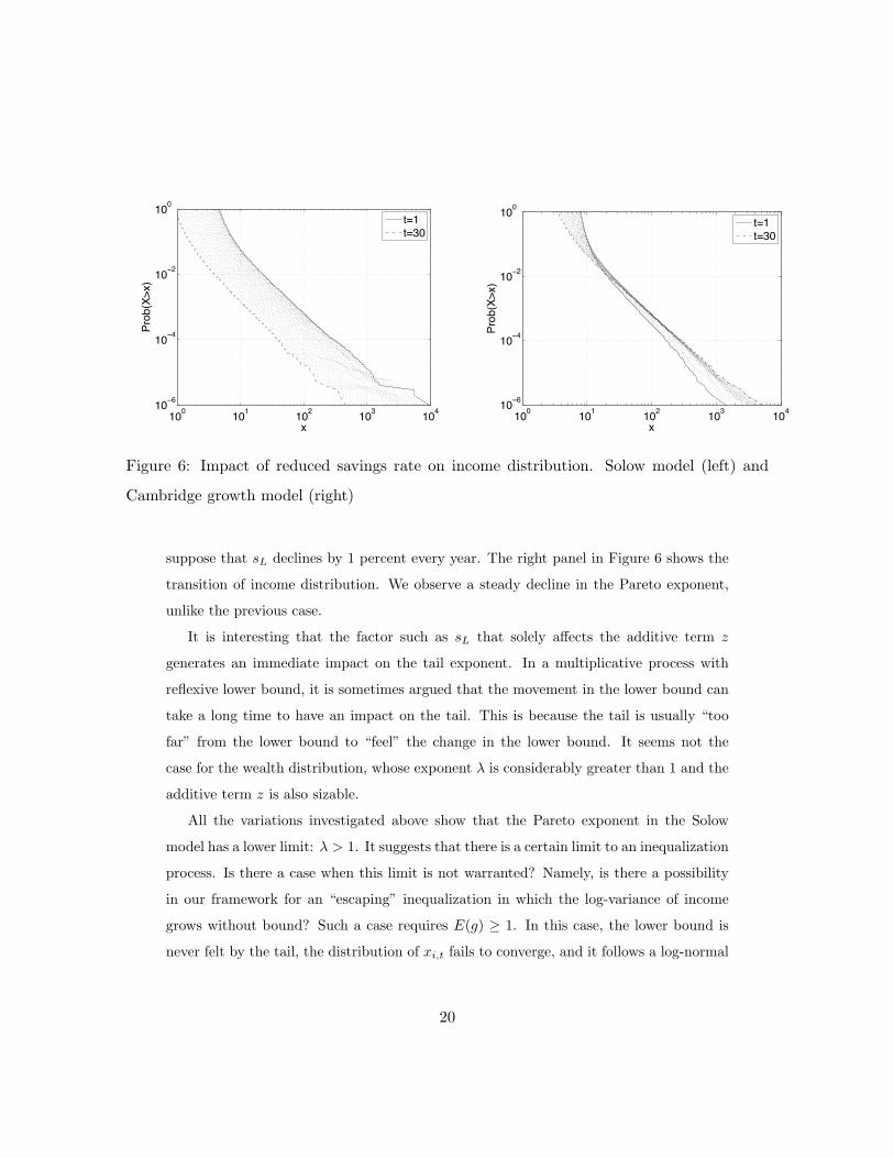
Figure 6: Impact of reduced savings rate on income distribution. Solow model (left) and
Cambridge growth model (right)
suppose that sL declines by 1 percent every year. The right panel in Figure 6 shows the
transition of income distribution. We observe a steady decline in the Pareto exponent,
unlike the previous case.
It is interesting that the factor such as sL that solely affects the additive term z
generates an immediate impact on the tail exponent. In a multiplicative process with
reflexive lower bound, it is sometimes argued that the movement in the lower bound can
take a long time to have an impact on the tail. This is because the tail is usually “too
far” from the lower bound to “feel” the change in the lower bound. It seems not the
case for the wealth distribution, whose exponent λ is considerably greater than 1 and the
additive term z is also sizable.
All the variations investigated above show that the Pareto exponent in the Solow
model has a lower limit: λ > 1. It suggests that there is a certain limit to an inequalization
process. Is there a case when this limit is not warranted? Namely, is there a possibility
in our framework for an “escaping” inequalization in which the log-variance of income
grows without bound? Such a case requires E(g) ≥ 1. In this case, the lower bound is
never felt by the tail, the distribution of xi,t fails to converge, and it follows a log-normal
20

development with log-variance linearly increasing in time.
Sources for such an escaping case are limited. It requires E(g) ≥ 1, namely, the
mean returns to wealth is greater than the overall growth rate of the economy. This
could happen in an extreme case like, say, when the investment is heavily subsidized
and financed by labor income tax. The Cambridge growth model studied above provides
an interesting alternative case. Consider a simple case sK = 1 and sL = 0 in which
the capital income is all reinvested and the labor income is all consumed. Then, the
wealth accumulation process (16) becomes a pure multiplicative process. The income
distribution follows a log-normal development, the log-variance of income grows linearly
in time, and the Pareto exponent falls toward zero. Whereas the assumption sK = 1 and
sL = 0 is extreme, this seems worth noting once we recall that the personal savings rate
in the U.S. experiences values below zero recently.
4 Ramsey model
In the previous section, we note the possibility that the different savings behavior across
the wealth group may have important implications on the Pareto exponent. In order to
pursue this issue, we need to depart from the Solow model and incorporate optimization
behavior of households. We work in a Ramsey model in this section. The model is
analytically tractable when the savings rate and portfolio decisions are independent of
wealth levels. Since Samuelson [26] and Merton [18], we know that this is the case
when the utility exhibits a constant relative risk aversion. We draw on Angeletos [2] in
which Aiyagari model [1] is modified to incorporate undiversifiable investment risks. Each
consumer is endowed with an initial capital ki,0, and a “backyard” production technology
that is the same as before (1). The labor endowment is constant at 1 and supplied
inelastically.
Households can engage in lending and borrowing bi,t at the risk-free interest Rt. Labor
can be hired at wage wt. The labor contract is contingent on the realization of the
technology shock ai,t. We assume that there is a small chance µ by which household
lineage is discontinued at each i. At this event, a new household is formed at the same
21

index i with no non-human wealth. Following the perpetual youth model [3], we assume
that households participate in a pension program. Households contract all of the non-
human wealth to be taken by the pension program at the event of discontinued lineage,
and they receive in return the premium in each period of continued lineage at rate p per
each unit of non-human wealth they own.
In each period, a household maximizes its profit from physical capital πi,t = yi,t−wtli,tsubject to the production function (1). At the optimal labor hiring li,t, the return to
capital is:
ri,t ≡ α(1− α)(1−α)/α(ai,t/wt)(1−α)/α + 1− δ. (33)
Household’s non-human wealth is defined as Fi,t ≡ ri,tki,t + Rtbi,t. Household’s total
wealth Wi,t is defined as:
Wi,t ≡ (1 + p)Fi,t +Ht (34)
= (1 + p)(ri,tki,t +Rtbi,t) +Ht (35)
where p is the pension premium and Ht is the human wealth defined as the expected
discounted present value of future wage income stream:
Ht ≡∞∑τ=t
wτ (1− µ)τ−tτ∏
s=t+1
R−1s . (36)
The evolution of the human wealth satisfies Ht = wt + (1 − µ)R−1t+1Ht+1. The pension
program is a pure redistribution system, and must satisfy the zero-profit condition: (1−
µ)p∫Fi,tdi = µ
∫Fi,tdi. Thus, the pension premium rate is determined at:
p = µ/(1− µ). (37)
Given an optimal operation of physical capital in each period, a household solves the
following dynamic maximization problem:
maxci,t,bi,t,ki,t+1
E0
( ∞∑t=0
βtc1−θi,t
1− θ
)(38)
subject to:
ci,t + ki,t+1 + bi,t+1 = ri,tki,t +Rtbi,t + wt (39)
22

and the no-Ponzi-game condition. For this maximization problem, consumption ci,t is
set at zero once the household lineage is discontinued. Using Ht and Wt, the budget
constraint is rewritten as:
ci,t + ki,t+1 + bi,t+1 + (1− µ)R−1t+1Ht+1 = Wi,t. (40)
Consider a balanced growth path at which Rt is constant over time. The household’s
problem has a recursive form:
V (Wi) = maxci,k′i,b
′i,W ′
i
c1−θi
1− θ+ (1− µ)βE (V (W ′i )) (41)
subject to
Wi = ci + k′i + b′i + (1− µ)R−1H ′ (42)
Wi = (1 + p)(riki +Rbi) +H. (43)
This dynamic programming allows the following solution as shown in Appendix D:
c = (1− s)W (44)
k′ = sφW (45)
b′ = s(1− φ)W − (1− µ)R−1H ′. (46)
Define xi,t ≡ Wi,t/γt as household i’s detrended total wealth. By substituting the
policy functions in the definition of wealth (35), and by noting that (1 − µ)(1 + p) = 1
holds from the zero-profit condition for the pension program (37), we obtain the equation
of motion for the individual total wealth:
x′i = g′ixi (47)
where the growth rate is defined as:
g′i ≡(φr′i + (1− φ)R)s
(1− µ)γ. (48)
Thus, at the balanced growth path, the household wealth evolves multiplicatively accord-
ing to (47) as long as the household lineage is continued. When the lineage is discontinued,
23

a new household with initial wealth Wi = H replaces the old one. Therefore, the indi-
vidual wealth Wi follows a log-normal process with random reset events where H is the
resetting point. Using the result of Manrubia and Zanette [17], we can establish the
Pareto exponent of the wealth distribution.
Proposition 6 A household’s detrended total wealth xi,t has a stationary Pareto distri-
bution with exponent λ which is determined by:
(1− µ)E(gλi,t) = 1. (49)
Proof: See Appendix E.
The result is quite comparable to the previous results in the Solow model. The
difference is that we do not have the additive term in the accumulation of wealth and
instead we have a random reset event. As seen in (49), the Pareto exponent is large when
µ is large. If there is no discontinuation event (i.e., µ = 0), then the individual wealth
follows a log-normal process as in [2]. In that case, the relative wealth Wi,t/∫Wj,tdj does
not have a stationary distribution. Eventually, a vanishingly small fraction of individuals
possesses almost all the wealth. This is not consistent with the empirical evidence.
The difference from the Solow model occurs from the fact that the consumption func-
tion is linear in income in the Solow model whereas it is linear in wealth in the Ramsey
model with CRRA preference. The linear consumption function arises in a quite narrow
specification of the Ramsey model, however, as Carroll and Kimball [5] argues. For ex-
ample, a concave consumption function with respect to wealth arises when labor income
is uncertain or when the household’s borrowing is constrained.
The concavity of the consumption means that the savings rate is high for the house-
holds with low wealth. This precautionary savings by the low wealth group serves as the
reflexive lower bound of the wealth accumulation process. Then, the Pareto exponent of
the tail distribution of wealth is determined by the balance of the precautionary savings
and the diffusion of the wealth as in the Solow model. Further analysis requires numerical
simulation, however, which is out of scope of the present paper.
24

5 Conclusion
This paper demonstrates that the Solow model with idiosyncratic investment risks is
able to generate the Pareto distribution as the stationary distribution of income at the
balanced growth path. We explicitly determine the Pareto exponent by the fundamental
parameters, and provide an economic interpretation for its determinants.
The Pareto exponent is determined by the balance between the two factors: the
savings from labor income, which determines the influx of population from the middle
class to the tail part, and the asset income contributed by risk-taking behavior, which
corresponds to the inequalizing diffusion effects taking place within the tail part. We
show that an increase in the variance of the idiosyncratic investment shock lowers the
Pareto exponent, while an increase in the technological growth rate raises the Pareto
exponent. Redistribution policy financed by income or bequest tax raises the Pareto
exponent, because the tax reduces the diffusion effect. Similarly, an increased level of
risk-sharing raises the Pareto exponent. Savings rate per se does not affect the Pareto
exponent, but a reduced savings rate from labor income lowers the Pareto exponent in a
model of differential savings rate.
The effect of different savings behavior across wealth groups can be investigated in a
Ramsey model. As a framework for such future studies, we present a Ramsey model with
CRRA utility which is analytically tractable but in which the savings rate is constant
across wealth groups. By incorporating a random event by which each household lineage
is discontinued, we reestablish the Pareto distribution of wealth and income.
Appendix
A Proof of Proposition 2
We first show that E(gλi,t) is strictly increasing in λ for σ > σ. This property is needed
to show the unique existence of λ as well as to be the basis of all the comparative statics
we conduct in this paper.
As λ→∞, gλ is unbounded for the region g > 1 and converges to zero for the region
25
g < 1, while the probability of g > 1 is unchanged. Thus E(gλ) grows greater than
1 eventually as λ increases to infinity. Also recall that E(g) < 1. Thus, E(gλ) travels
from below to above 1. Hence, there exists unique λ that satisfies E(g) = 1 if E(gλ) is
monotone in λ, and the solution satisfies λ > 1.
To establish the monotonicity, we show that the first derivative of the moment (d/dλ)E(gλ) =
E(gλ log g) is strictly positive. Since (d/dλ)(gλ log g) = gλ(log g)2 > 0, we have E(gλ log g) ≥
E(g log g). Denote g = a + u where a = (1 − δ)/γ and log u follows a normal dis-
tribution with mean µu = u0 − σ2u/2 and variance σ2
u = ((1 − α)/α)2σ2 where u0 ≡
log(α(1− (1− δ)/γ)). Then, noting that a > 0 and u > 0, we obtain:
E(g log g) = aE(log(a+ u)) + E(u log(a+ u)) > a log a+ E(u log u). (50)
The last term is calculated as follows:∫ ∞0
u log uuσu√
2πe− (log u−µu)2
2σ2u du =
∫ ∞0
log uuσu√
2πe− (log u−µu)2−2σ2
u log u
2σ2u du (51)
= eµu+σ2u/2
∫ ∞0
log uuσu√
2πe− (log u−(µu+σ2
u))2
2σ2u du (52)
= eµu+σ2u/2(µu + σ2
u). (53)
Collecting terms, we obtain:
E(g log g) >1− δγ
log1− δγ
+ α
(1− 1− δ
γ
)(log(α
(1− 1− δ
γ
))+σ2
2
(1− αα
)2).
(54)
Since 1− (1− δ)/γ > 0, the right hand side is positive for a sufficiently large σ. Thus, by
defining:
σ2 ≡log[(
1−δγ
)− 1−δγ(α(
1− 1−δγ
))−α(1− 1−δγ )]
α2
(1− 1−δ
γ
) (1−αα
)2 , (55)
we obtain that E(g log g) is positive for σ ≥ σ. Thus, E(gλ) is strictly increasing in λ
under the sufficient condition σ ≥ σ.
Finally, we show that λ is decreasing in σ by showing that an increase in σ is a mean-
preserving spread in g. Recall that g follows a shifted log-normal distribution where
log u = log(g − a) follows a normal distribution with mean u0 − σ2u/2 and variance σ2
u.
26

Note that the distribution of u is normalized so that a change in σu is mean-preserving
for g. The cumulative distribution function of g is F (g) = Φ((log(g−a)−u0 +σ2u/2)/σu)
where Φ denotes the cumulative distribution function of the standard normal. Then:
∂F
∂σu= φ
(log(g − a)− u0 + σ2
u/2σu
)(− log(g − a)− u0
σ2u
+12
)(56)
where φ is the derivative of Φ. By using the change of variable x = (log(g − a) − u0 +
σ2u/2)/σu, we obtain:∫ g ∂F
∂σudg =
∫ x
φ(x)(−x/σu + 1)dxdg/dx (57)
= σueu0
∫ x −x/σu + 1√2π
e−(x−σu)2/2dx (58)
The last line reads as a partial moment of −x/σu + 1 in which x follows a normal dis-
tribution with mean σu and variance 1. The integral tends to 0 as x → ∞, and it is
positive for any x below σu. Thus, the partial integral achieves the maximum at x = σu
and then monotonically decreases toward 0. Hence, the partial integral is positive for
any x, and so is∫ g∂F/∂σudg. This completes the proof for that an increase in σu is a
mean-preserving spread in g. Since gλ is strictly convex in g for λ > 1, a mean-preserving
spread in g strictly increases E(gλ). As we saw, E(gλ) is also strictly increasing in λ.
Thus, an increase in σu, and thus an increase in σ while α is fixed, results in a decrease
in λ that satisfies E(gλ) = 1 in the region λ > 1.
B Derivation of Equation (22)
We repeatedly use the fact that, when log ε follows a normal distribution with mean
−σ2/2 and variance σ2, a0 log ε also follows a normal with mean −a0σ2/2 and variance
a20σ
2. When δ = 1, the growth rate of xi,t becomes a log-normally distributed variable
g = αε(1−α)/α/E(ε(1−α)/α). Then, gλ also follows a log-normal with log-mean λ(logα −
log E(ε(1−α)/α)− (σ2/2)((1−α)/α)) and log-variance λ2((1−α)/α)2σ2. Then we obtain:
1 = E(gλ) = eλ(logα−log E(ε(1−α)/α)−(σ2/2)((1−α)/α))+λ2((1−α)/α)2σ2/2 (59)
= eλ(logα−(σ2/2)((1−α)/α)2)+λ2((1−α)/α)2σ2/2. (60)
27

Taking logarithm of both sides, we solve for λ as:
λ = 1−(
α
1− α
)2 logασ2/2
. (61)
C Proof of Proposition 3
From the definition of gi,t (17), we obtain:
E(g2i,t) =
(1− δγ
)2
+ 21− δγ
α
γ(γ − 1 + δ) +
(α
γ(γ − 1 + δ)
)2 E(ε2(1−α)/αi,t )(
E(ε(1−α)/αi,t )
)2 . (62)
By applying the formula for the log-normal, we obtain:
E(ε2(1−α)/αi,t )(
E(ε(1−α)/αi,t )
)2 =e−σ
2(1−α)/α+2σ2(1−α)2/α2
e−σ2(1−α)/α+σ2(1−α)2/α2 = e
(σ(1−α)α
)2(63)
Combining these results with the condition E(g2) = 1, we obtain:
σ2 =(
α
1− α
)2
log(
1α2
(1− 2α
γ/(1− δ)− 1
)). (64)
We observe that an increase in γ or δ raises σ. By Proposition 2, E(gλ) is monotonically
increasing in λ when σ > σ, and λ is decreasing in σ. Thus, in the neighborhood of λ = 2,
the stationary λ is increasing in γ or δ, because an increase in either of them raises σ
relative to the current level of σ.
D Derivation of the policy function in the Ramsey
model
First, we guess and verify the policy functions (44,45,46) at the balanced growth path
along with a guess on the value function V (W ) = BW 1−θ/(1 − θ). The guessed policy
functions for c, k′, b′ are consistent with the budget constraint (42).
The first order conditions and the envelope condition for the Bellman equation (41)
are:
c−θ = βE[r′V ′(W ′)] (65)
28

c−θ = βRE[V ′(W ′)] (66)
V ′(W ) = c−θ (67)
Note that we used the condition (1− µ)(1 + p) = 1 from (37). By imposing the guess on
these conditions, and by using W ′ = (φr′+ (1−φ)R)(1 + p)sW from (47), we obtain the
equations that determine the constants:
0 = E[(r′ −R)(φr′ + (1− φ)R)−θ] (68)
s = (1− µ)(βE[r′(φr′ + (1− φ)R)−θ]
)1/θ(69)
B = (1− s)−θ. (70)
Thus we verify the guess.
E Proof of Proposition 6
In this section, we solve the Ramsey model and show the existence of the balanced growth
path. Then the proposition obtains directly by applying Manrubia and Zanette [17].
At the balanced growth path, Y , K, and wealth grow at the same rate γ. The wage
and output are determined similarly to the Solow model (7,8). As in the Solow model,
define Xt = Kt/γt as detrended aggregate physical capital. At the steady state X, the
return to physical capital (33) is written as:
ri,t = αε(1−α)/αi,t E(ε(1−α)/α
i,t )α−1Xα−1 + 1− δ, (71)
which is a stationary process. The average return is:
r ≡ E(r) = αηXα−1 + 1− δ. (72)
The lending market must clear in each period, which requires∫bi,tdi = 0 for any
t. By aggregating the non-human wealth and using the market clearing condition for
lending, we obtain:∫Fi,tdi = rKt. Thus the aggregate total wealth satisfies
∫Wi,tdi =
(1 − µ)−1rKt + Ht. At the balanced growth path, aggregate total wealth, non-human
wealth and human wealth grow at rate γ. Let W , H, and w denote the aggregate total
29

wealth, the human capital and the wage rate detrended by γt at the balanced growth
path, respectively. Then we have:
W = (1− µ)−1rX + H. (73)
Combining the market clearing condition for lending with the policy function for lending
(46), we obtain the equilibrium risk-free rate:
R =γ(1− µ)s(1− φ)
H
W. (74)
By using the conditions above and substituting the policy function (44), the budget
constraint (40) becomes in aggregation:
(γ − s(1− µ)−1r)X = (s− (1− µ)R−1γ)H. (75)
Plugging into (74), we obtain the relation:
R =γ(1− µ)s(1− φ)
− φ
1− φr. (76)
Thus, the mean return to the risky asset and the risk-free rate are determined by X from
(72,76). The expected excess return is solved as:
r −R =1
1− φ(αηXα−1 + 1− δ − (1− µ)γ/s
). (77)
If log ε ∼ N(−σ2/2, σ2), then we have η = eσ22 (1−α)(1/α−2). This shows a relation between
the expected excess return and the shock variance σ2.
By using (7,8), the human wealth is written as:
H = γ−t
( ∞∑τ=t
wγτ (1− µ)τ−tτ∏
s=t+1
R−1s
)=
w
1− (1− µ)γR−1=
(1− α)ηXα
1− (1− µ)γR−1.
(78)
Equations (72,75,76,78) determine X, H, R, r. In what follows, we show the existence
of the balanced growth path in the situation when the parameters of the optimal policy
s, φ reside in the interior of (0, 1). By using (72,76,78), we have:
X
H=
1− (1−µ)γs(1−φ)γ(1−µ)−sφ(1−δ)−sφαηXα−1
(1− α)ηXα−1. (79)
30

The right hand side function is continuous and strictly increasing in X, and travels from
0 to +∞ as X increases from 0 to +∞.
Now, the right hand side of (75) is transformed as follows:
H(s− (1− µ)γR−1) = H
(s− s(1− φ)
W
H
)= Hs
(1− (1− φ)
((1− µ)−1 rX
H+ 1))
= Hs
(φ− (1− φ)(1− µ)−1 rX
H
). (80)
Then we rearrange (75) as:
γ
sφ
X
H= 1 + (1− µ)−1 rX
H. (81)
By (72), r is strictly decreasing in X, and R is strictly increasing by (76). Thus W/H
is strictly decreasing by (74), and so is rX/H by (73). Thus, the right hand side of (81)
is positive and strictly decreasing in X. The left hand side is monotonically increasing
from 0 to +∞. Hence there exists the steady-state solution X uniquely. This verifies the
unique existence of the balanced growth path.
The law of motion (47) for the detrended individual total wealth xi,t is now completely
specified at the balanced growth path:
xi,t+1 =
gi,t+1xi,t with prob. 1− µ
H with prob. µ,(82)
where,
gi,t+1 ≡ (φri,t+1 + (1− φ)R)s/((1− µ)γ). (83)
This is the stochastic multiplicative process with reset events studied by Manrubia and
Zanette [17]. By applying their result, we obtain our proposition.
References
[1] S. Rao Aiyagari. Uninsured idiosyncratic risk and aggregate saving. Quarterly Jour-
nal of Economics, 109:659–684, 1994.
[2] George-Marios Angeletos. Uninsured idiosyncratic investment risk and aggregate
saving. Review of Economic Dynamics, 10:1–30, 2007.
31

[3] Olivier J. Blanchard. Debt, deficits, and finite horizons. Journal of Political Econ-
omy, 93:223–247, 1985.
[4] Alan S. Blinder. A model of inherited wealth. Quarterly Journal of Economics,
87:608–626, 1973.
[5] Christopher D. Carroll and Miles S. Kimball. On the concavity of the consumption
function. Econometrica, 64:981–992, 1996.
[6] Ana Castaneda, Javier Dıaz-Gimenez, and Jose-Victor Rıos-Rull. Accounting for
the U.S. earnings and wealth inequality. Journal of Political Economy, 111:818–857,
2003.
[7] D.G. Champernowne. A model of income distributon. Economic Journal, 63:318–
351, 1953.
[8] Jayasri Dutta and Philippe Michel. The distribution of wealth with imperfect altru-
ism. Journal of Economic Theory, 82:379–404, 1998.
[9] Daniel R. Feenberg and James M. Poterba. Income inequality and the incomes of
very high income taxpayers: Evidence from tax returns. In James M. Poterba, editor,
Tax Policy and the Economy, pages 145–177. MIT Press, 1993.
[10] William Feller. An Introduction to Probability Theory and Its Applications, vol-
ume II. Wiley, NY, second edition, 1966.
[11] Y. Fujiwara, W. Souma, H. Aoyama, T. Kaizoji, and M. Aoki. Growth and fluctua-
tions of personal income. Physica A, 321:598–604, 2003.
[12] Xavier Gabaix. Zipf’s law for cities: An explanation. Quarterly Journal of Eco-
nomics, 114:739–767, 1999.
[13] Mark Huggett. Wealth distribution in life-cycle economies. Journal of Monetary
Economics, 38:469–494, 1996.
[14] M. Kalecki. On the Gibrat distribution. Econometrica, 13:161–170, 1945.
[15] Harry Kesten. Random difference equations and renewal theory for products of
random matrices. Acta Mathematica, 131:207–248, 1973.
32

[16] M. Levy and S. Solomon. Power laws are logarithmic boltzmann laws. International
Journal of Modern Physics C, 7:595, 1996.
[17] Susanna C. Manrubia and Demian H. Zanette. Stochastic multiplicative processes
with reset events. Physical Review E, 59:4945–4948, 1999.
[18] Robert C. Merton. Lifetime portfolio selection under uncertainty: The continuous-
time case. Review of Economics and Statistics, 51:247–257, 1969.
[19] Elliott W. Montroll and Michael F. Shlesinger. Maximum entropy formalism, frac-
tals, scaling phenomena, and 1/f noise: A tale of tails. Journal of Statistical Physics,
32:209–230, 1983.
[20] Chiaki Moriguchi and Emmanuel Saez. The evolution of income concentration in
japan, 1886-2005: Evidence from income tax statistics. Review of Economics and
Statistics, 90:713–734, 2008.
[21] M.E.J. Newman. Power laws, pareto distributions and zipf’s law. Contemporary
Physics, 46:323–351, 2005.
[22] Makoto Nirei and Wataru Souma. A two factor model of income distribution dy-
namics. Review of Income and Wealth, 53:440–459, 2007.
[23] Pierre Pestieau and Uri M. Possen. A model of wealth distribution. Econometrica,
47:761–772, 1979.
[24] Thomas Piketty and Emmanuel Saez. Income inequality in the United States, 1913-
1998. Quarterly Journal of Economics, CXVIII:1–39, 2003.
[25] R.S.G. Rutherford. Income distribution: A new model. Econometrica, 23:277–294,
1955.
[26] Paul A. Samuelson. Lifetime portfolio selection by dynamic stochastic programming.
Review of Economics and Statistics, 51:239–246, 1969.
[27] J. D. Sargan. The distribution of wealth. Econometrica, 25:568–590, 1957.
[28] A. F. Shorrocks. On stochastic models of size distributions. Review of Economic
Studies, 42:631–641, 1975.
33

[29] H.A. Simon. On a class of skew distribution functions. Biometrika, 52:425–440,
1955.
[30] W. Souma. Physics of personal income. In H. Takayasu, editor, Empirical Science
of Financial Fluctuations. Springer-Verlag, 2002.
[31] J. E. Stiglitz. Distribution of income and wealth among individuals. Econometrica,
37:382–397, 1969.
[32] R. N. Vaughan. Class behaviour and the distribution of wealth. Review of Economic
Studies, 46:447–465, 1979.
[33] H. O. A. Wold and P. Whittle. A model explaining the Pareto distribution of wealth.
Econometrica, 25:591–595, 1957.
34