Embed Size (px)
Citation preview

11/28/06 - User Manual for the PARCS Neutronics Core Simulator - 2
PARCS v2.7 U.S. NRC Core Neutronics Simulator
USER MANUAL
November, 2006
T. DownarY. Xu V. Seker
School of Nuclear Engineering
Purdue University
W. Lafayette, Indiana 47907
D. Carlson
RES / U.S. NRC Rockville, Md

11/28/06 - User Manual for the PARCS Neutronics Core Simulator - 3
TABLE OF CONTENTS
I. INTRODUCTION ..................................................................................................................3
II. PARCS FEATURES...............................................................................................................5II.A Calculation Features..................................................................................................5II.B Modeling Features.....................................................................................................7II.C Input Features..........................................................................................................10II.D Output Features .......................................................................................................13
III. METHODS OVERVIEW.....................................................................................................21III.A Spatial Discretization Methods .............................................................................21
III.A.1 Nonlinear CMFD Method .........................................................................21III.A.2 Nodal Method ............................................................................................23III.A.3 Pin Power Reconstruction .........................................................................23III.A.4 Control Rod Cusping Correction ..............................................................23III.A.5 1D Nodal Kinetics.......................................................................................24III.A.6 Hexagonal Geometry .................................................................................25III.A.7 Fine Mesh Finite Difference Kernel ..........................................................25III.A.8 SP3 Transport Kernel ................................................................................26
III.B Temporal Differncing ............................................................................................26III.C Control Rod Scram Logic ..........................................................................................III.D Restart Capability .....................................................................................................III.E Neutronic vrs T-H Variable Mapping .......................................................................III.F Automatic Mapping ...............................................................................................27III.G Core Depletion Analysis .........................................................................................28
IV. EXECUTING PARCS..........................................................................................................31IV.A Execution Modes.....................................................................................................31IV.B PARCS Execution Procedure..................................................................................32
V. INPUT DESCRIPTION........................................................................................................34V.A PARCS Input Card Description ..............................................................................34V.B MAPTAB Input Description...................................................................................72
VI. SAMPLE INPUTS................................................................................................................95VI.A OECD MSLB Benchmark ......................................................................................95VI.B BWR Peach Bottom Turbine Trip Benchmark .....................................................106VI.C VVER1000 Rod Ejection Benchmark ..................................................................115
VII. SAMPLE OUTPUTS..........................................................................................................117VII.A OECD MSLB Benchmark ....................................................................................117VII.B BWR Peach Bottom Turbine Trip Benchmark .....................................................122VII.C VVER1000 Rod Ejection Benchmark ..................................................................124
VIII. REFERENCES ...................................................................................................................128
TABLE OF CONTENTS
11/28/06 - Volume 2: User Manual for the PARCS Kinetics Core Simulator Module - 4
I. INTRODUCTION
PARCS is a three-dimensional (3D) reactor core simulator which solves the steady-state andtime-dependent, multi-group neutron diffusion and SP3 transport equations in orthogonal andnon-orthogonal geometries. PARCS is coupled directly to the thermal-hydraulics system codeTRACE which provide the temperature and flow field information to PARCS during the transientcalculations via the few group cross sections. A separate code module, GENPMAXS, is used toprocess the cross sections generated by a lattice physics code into the PMAXS format that can beread by PARCS.
Since the initial release of the NRC version of PARCS (V1.01) in November 1998 [1], therehave been numerous functional improvements and code feature extensions. The features will besummarized in section III and more detailed description is provided in the PARCS Theory Man-ual. The major calculation features in PARCS include the ability to perform eigenvalue calcula-tions, transient (kinetics) calculations, Xenon transient calculations, decay heat calculations, pinpower calculations, and adjoint calculations for commercial Light Water Reactors. The primaryuse of PARCS involves a 3D calculation model for the realistic representation of the physicalreactor. However, various one-dimensional (1D) modeling features are available in PARCS tosupport faster simulations for a group of transients in which the dominant variation of the flux isin the axial direction, as for example in several BWR applications.
A card name based input system is employed in PARCS such that the use of default inputparameters is maximized and the amount of the input data is minimized. A restart feature is avail-able to continue the transient calculation from the point where the restart file was written. Variousedit options are available in PARCS to show many different aspects of the calculation results.The on-line graphics feature of PARCS provides a quick and versatile visualization of the variousphysical phenomena occurring during the transient calculation. These PARCS features aredescribed in detail in the subsequent sections.
Numerous sophisticated spatial kinetics calculation methods have been incorporated intoPARCS in order to accomplish the various tasks with high accuracy and efficiency. For example,the CMFD formulation provides a means of performing a fast transient calculation by avoidingexpensive nodal calculations at times in the transient when there is no strong variation in the neu-tron flux spatial distribution. The temporal discretization is performed using the theta methodwith an exponential transformation of the group fluxes. A transient fixed source problem isformed and solved at each time point in the transient. For spatial discretization, a variety of solu-tion kernels are available to include the most popular LWR two group nodal methods, ANM [7]and NEM.
Advanced numerical solution methods are used in PARCS in order to minimize the compu-tational burden. The solution of the CMFD linear system is obtained using a Krylov subspacemethod which utilizes a BILU3D preconditioner [8]. The eigenvalue calculation to establish theinitial steady-state is performed using the Wielandt eigenvalue shift method. When using the twogroup nodal methods, a pin power reconstruction method is available in which predefined hetero-geneous power form functions are combined with a homogeneous intranodal flux distribution [9].
For 1D calculations, two modes are available in PARCS: normal 1D and quasistatic 1D. Thenormal 1D mode uses a 1D geometry and precollapsed 1D group constants, while the quasistatic
11/28/06 - Volume 2: User Manual for the PARCS Kinetics Core Simulator Module - 5
1D keeps the 3D geometry and cross sections, but performs the neutronic calculation in the 1Dmode using group constants which are collapsed during the transient. The group constants to beused in PARCS 1D calculation can be generated through a set of 3D PARCS calculations. Duringthe 1D group constant generation, “current conservation” factors are employed in the PARCS 1Dcalculations to preserve the 3D planar averaged currents in the subsequent 1D calculations. Anoverview of the methods employed in PARCS is given in Section III in order to assist users inchoosing the calculation options most suitable to their application.
PARCS is also capable of performing core depletion analysis. Burnup dependent macro-scopic cross sections are read from the PMAXS file prepared by the code GENPMAXS and thePARCS node-wise power is used to calculate the region-wise burnup increment for time advanc-ing the macroscopic cross sections. Details of the PMAXS file and the GENPMAXS code areprovided in the GENPMAXS manual.
PARCS was written in FORTRAN90 and its portability has been tested on various platformsand operating systems, to include SUN Solaris Unix, DEC Alpha Unix, HP Unix, LINUX, andvarious Windows OS (i.e. 95, 98, NT, and 2000).Because of its various functional features,PARCS can be run in numerous execution modes as summarized in Section IV. The rules of thePARCS input system are summarized in Section V. Several sample problems with their appropri-ate inputs and outputs are provided in Section VI and Section VII. The following section will firstprovide a brief overview of the important PARCS user features.
II. PARCS FEATURES
The features of PARCS can be categorized into calculations, modeling, and I/O features.The calculation features cover what type of internal calculations can be performed by PARCS,e.g. eigenvalue calculation or kinetics calculations. The modeling features cover what type ofinput models can be used in PARCS, e.g. 3D vs. 1D. Lastly, the I/O features cover the input sys-tem and output features of PARCS, e.g. the card name-based input system and on-line graphics.This section describes all the PARCS features according to this classification. Some input cardsrelevant to the feature being described here will be mentioned along with the input block name towhich they belong. Note that the detailed input system and card description is given in Section IV.
II.A Calculation Features
PARCS is equipped with various calculation modules needed for predicting the global andlocal response of the reactor in steady-state and transient conditions. The various features ofPARCS are described in this section along with the corresponding modules.
II.A.1 Eigenvalue Calculation
In order to establish the initial steady-state, it is necessary to perform an eigenvalue calcula-tion. PARCS performs the eigenvalue calculation using the Wielandt eigenvalue shift method.The eigenvalue obtained is used to adjust the nu values in the subsequent transient calculation tomake the initial state critical. In addition to the standard k-eff calculation for a given reactor con-

11/28/06 - Volume 2: User Manual for the PARCS Kinetics Core Simulator Module - 6
figuration, the critical boron concentration (CBC) search function is available. The type ofsearch is defined in the SEARCH card of the CNTL block input.
II.A.2 Transient Calculation
This is the primary function of PARCS that solves the time-dependent neutron diffusionequations involving both delayed and prompt neutrons. The temporal differencing based on theexponential transform and the theta method yields a transient fixed source problem at each timepoint. The fixed source problem is solved by the CMFD method in which a conditional nodalupdate scheme is employed. The temporal discretization schemes can be specified by theTHETA and EXPO_OPT cards in the TRAN input block. Exponential extrapolation to obtain aninitial guess at the new time step is also available in the expo_opt card. The conditional updatescheme invokes the “expensive” nodal update only when there are substantial local cross sectionchanges. The control of the conditional update is done by the EPS_XSEC card in the TRANblock. The transient calculation option is turned on and off by the TRANSIENT card in theCNTL block.
II.A.3 Xenon/Samarium Calculation
For the slow and long lasting transient, a Xenon transient calculation is essential. In thiscase, a quasistatic transient calculation method that employes the eigenvalue problem solverinstead of the transient fixed source problem is used and the number densities of Xenon andSamarium are updated by solving the respective balance equations using the fluxes resulting fromthe eigenvalue calculation. The Xenon option is specified in the XE_SM card in the CNTL blockto choose one of 1) No Xenon, 2) Equilibrium Xenon, or 3) Transient Xenon options.
II.A.4 Decay Heat Calculation
A simplified decay heat model involving six groups of decay heat precursor groups [10] isemployed in PARCS. The 6 group decay heat precursor equation is treated in the same way asthe delayed neutron precursor equation. The solution of the precursor equation is thus made foreach node and provides the decay heat at each time step to be summed with the fission power toproduce the total power. Default values of the fraction and decay constant of the 6 groups are pro-vided for the UO2 cores operated for a sufficiently long period of time. The user can also specifyvalues. The decay heat option is specified in the DECAY_HEAT card in the CNTL block and theinput parameters are specified in the DHP_BETA and DHP_LAMBDA cards in the XSECblock.
II.A.5 Pin Power Calculation
The primary unknown in the PARCS nodal solution kernel is the node average flux. In orderto obtain local pin power distributions, it is thus necessary to “reconstruct” pin powers from thenode average flux values. This is achieved in PARCS by multiplying the heterogeneous power

11/28/06 - Volume 2: User Manual for the PARCS Kinetics Core Simulator Module - 7
form functions by the homogeneous intranodal flux distribution. The homogeneous intranodalflux is calculated by finding the analytic solution of a 2D fixed source problem in which the sur-face average currents are specified at the four boundaries. The surface average currents areobtained from the converged node average flux distribution at a given state. The pin power recon-struction is performed for the transient conditions with transient fixed source as well as for thesteady-state conditions. The pin power calculation option is turned on and off by thePIN_POWER card in the CNTL block and the heterogeneous power form functions are suppliedvia the PFF block. Corner discontinuity factors can be used to enhance the accuracy of the pinpower distribution and they are specified in the CDF card in the XSEC block. In order to savecomputing time for pin power calculation, a subset of fuel assemblies can be selected for pinpower calculation in the PINCAL_LOC card in the GEOM block. The transient pin power calcu-lation need not be performed at every time step since the pin-to-box factor does not change muchunless there is a substantial change in the core configuration. The transient pin power calculationfrequency is specified by the PIN_FREQ card in the TRAN block.
II.A.6 Adjoint Calculation
The adjoint flux is needed for the reactivity edits during the transient calculation. For this,the adjoint calculation is performed at the end of the steady-state calculation with the transpose ofthe converged CMFD coefficient matrix. The adjoint option is turned on by the POPT(5) optionin the PRINT_OPT card in the CNTL block.
II.B Modeling Features
The essential problem of modeling is to represent a physical system with a numerical model.Among the various fundamental modeling issues in the reactor kinetics calculation are the geo-metric representation, the cross section representation, and the T-H modeling. PARCS provides a3D geometric representation that can be reduced to 2D, 1D, or 0D by the choice of the boundaryconditions. However, special 1D kinetics capabilities are also available for more accurate and ver-satile 1D modeling. Various geometric representation features will be described in the first andfourth subsections below. The basic cross section representation scheme in PARCS is to function-alize the macroscopic cross sections with linear or quadratic dependence on the T-H state vari-ables, and the details of the PARCS cross section representation schemes are given in the secondsubsection. Thermal-hydraulically, PARCS uses the TRACE code to obtain temperature/fluidfield information feedback, which greatly extends its applicability.
II.B.1 Geometric Representation
In PARCS, the reactor core is modeled by a group of homogeneous computational nodes.Radially, the size of the node is of the order of fuel assembly pitch, while axially the size is 15~30cm. In PARCS’s GEOM block, the core radial configuration is specified in the unit of assemblyby the RAD_CONF card in the GEOM block. The radial node size is then specified by the num-ber of subdivision of the assembly node by the NEUTMESH_X and NEUTMESH_Y cards. So

11/28/06 - Volume 2: User Manual for the PARCS Kinetics Core Simulator Module - 8
the number of nodes per assembly can be freely chosen as nsubx*nsuby. Normally, one or fournodes per assembly is used for practical calculations. However, in principle, it is possible to per-form a fine mesh calculation with the geometry input structure. Also by taking the assembly con-figuration as the pin configuration, a pin-by-pin heterogeneous core representation is alsopossible. The problem symmetry is determined by the boundary conditions specified at the twoboundaries in each direction in the BOUN_COND card in the GEOM block. Three boundaryconditions are available: zero current, zero flux, and zero incoming current. By choosing the zerocurrent option on the left side boundary, one can construct a quarter core or a half core symmetryproblem. By taking the top and bottom boundary conditions to be zero current, a 2D problem canbe constructed with one plane. Similarly, by taking all the radial boundary conditions to be zerocurrent, a 1D problem can be setup.
II.B.2 Cross Section Functionalization
PARCS uses macroscopic cross sections since it is not intended to perform any depletioncalculations. The macroscopic nodal cross sections are functionalized on boron concentration (B,in ppm), square root of the effective fuel temperature, moderator temperature and density, voidfraction and the effective rodded fractions . The effective fuel temperature can be pro-vided as either the volume average fuel temperature or the Doppler temperature using the Row-lands relation as described in reference [11] and in the PARCS Theory Manual. Only the lineardependence of cross sections is considered on these state variables except for the moderator den-sity and void fraction for which the quadratic variation is additionally considered. In terms ofsymbols, the cross sections are functionalized as:
(1)
The fuel temperature, , is the effective doppler fuel temperature and can be computed usingeither the volume average fuel temperature or a linear combination of the centerline and surfacetemperatures as described in Reference [11] and in the PARCS Theory Manual. The effectiverodded fraction is defined as the product of the volumetric rodded fraction and the flux depressionfactor that is computed by the decusping routine for the partially rodded node. For Xenon calcula-tions, the Xenon and Samarium microscopic cross sections are represented in the same form. Thebase cross sections and the proportionality constants are specified by the BASE_MACRO,DXS_DPPM, DXS_DTF, DXS_DTM, DXS_DDM, DXS_DDM2, DXS_DVOID,DXS_DVOID2, DELCR_BASE cards in the XSEC block. Special types of cross section repre-sentation for benchmark calculations are also available and are selected by the FUNC_TYPEcard in the XSEC block. Currently, two special benchmark cross section representation types areavailable: one for the OECD MSLB (Main Steam Line Break) problem and the other for theOECD PBTT (Peach Bottom Turbine Trip) problem. For 1D kinetics, more cross section repre-sentation schemes including table forms are available and these are discussed in Section II.B.4.
α( ) ξ( )
Σ B Tf Tm Dm α ξ, , , , ,( ) Σ0 a1 B B0–( ) a2 Tf Tf0–( ) a3 Tm Tm0–( )a4 Dm Dm0–( ) a5 Dm Dm0–( )2 a6α a7α
2 ξΔΣCR
+ + ++ + + + +
=
Tf
11/28/06 - Volume 2: User Manual for the PARCS Kinetics Core Simulator Module - 9
II.B.3 Thermal-Hydraulics Feedback
PARCS is coupled with the thermal-hydraulics code TRACE by the EXT_TH card in theCNTL block. The coupling between PARCS and the TRACE code is achieved by the interprocesscommunication protocol, PVM. The two processes are loaded in parallel and the PARCS processtransfers the nodal power data to the T-H process. The T-H process then sends back the tempera-ture (fuel and coolant) and density data back to the PARCS process. Originally, it was necessaryto execute a third intermediate process, GI, which manages the data transfer between the two pro-cesses. But this process has been integrated into PARCS in this release so that only two processesare to be run in parallel.
In general, the neutronic node structure is different from the T-H node structure. The differ-ence is to be mitigated by a proper mapping scheme. This mapping used to be explicit in that thefractions of different T-H nodes belonging to a neutronic node had to be specified in a file calledMAPTAB for all the neutronic nodes. In order to reduce the user effort to prepare the MAPTABfile, automatic mapping schemes were developed for the coupled TRACE/PARCS code that takedata from both PARCS and TRACE input files to generate the mapping information internally.
The time step size used in system T-H calculations is often small because of stability con-siderations. Some times it is so small that no significant changes occur in the core T-H conditionand performing a neutronic calculation with such a small change would be wasteful since the neu-tronics solution does not change much either. In order to circumvent this inefficiency, a skip fac-tor can be used in the coupled calculation such that the T-H code calls PARCS based on this user-defined frequency. Different skip factors can be specified for the steady state and transient calcu-lations in the EXT_TH card.
II.B.4 1D Kinetics
PARCS is equipped with 1D kinetics capabilities for faster execution of some axially domi-nated transients and also for providing the capability to execute existing TRAC-B 1D kineticsdecks. In addition, it has a quasi-static 1D kinetics capability in which the radial flux shape isassumed to be constant or linearly varying between specified points. Below, three 1D kinetics fea-tures available in PARCS are described.
Normal 1D Kinetics: This is the standard 1D kinetics calculation method based on the 1D groupconstants that were generated and functionalized via planar averaging from a set of 3D steady-state calculations at various core states. The normal 1D kinetics can be invoked by theONED_KIN card in the CNTL block. The 1D group constant can be functionalized by one of thethree possible options: a general table form, a polynomial form, and a linear form. The generaltable form takes the following representation in which the base and rodded cross sections are pro-vided as 2 dimensional tables where the two independent variables are the moderator density andthe square root of effective fuel temperature:

11/28/06 - Volume 2: User Manual for the PARCS Kinetics Core Simulator Module - 10
(2)
Note that it also has the boron correction term given only by coefficients. On the other hand thepolynomial cross section takes the following form that is consistent with the 1D formulation usedin the TRAC-B code.
(3)
The linear form is to use Eq. (1) as the 3D representation. The cross section form is selected bythe XS_FORM in the ONEDK block and the actual 1D cross section data are given in a separatefile designated by the EXT1DXS card in the ONEDK block. For accurate conservation of the 3Dplanar averaged currents in 1D calculation, so called current conservation factors (CCF) can beused in the 1D flux calculation. This option is selected by the USE_CCF card in the ONEDKblock. Even though the kinetics calculation is performed in 1D, it is possible to perform the T-Hcalculation in 3D with multiple flow channels. This is possible by assigning predefined radialpower shapes so that reconstruction of the 3D power distribution can be done using the planarpower determined in the 1D kinetics calculation. The RAD_WEIGHT and CHAN_AREA cardsin the ONEDK block are used for this purpose. Lastly, for 1D bare core modeling, an albedomatrix can be input at the top and bottom of the core with the ALBEDO_ZL and ALBEDO_ZRcards in the GEOM block.
TRAC-B 1D Kinetics: PARCS can take an existing TRAC-B input deck as the 1D kinetics inputfile. If a file name tracin exists in the working directory, no PARCS input files are required. Allthe kinetics input data are taken from the POW* cards provided in the tracin file.
Quasi-static 1D Kinetics: The quasi-static (QS) 1D kinetics feature is unique in PARCS and itrequires a normal 3D model including the geometry and the normal cross section data. The neu-tronics calculation is, however, performed in 1D using the 1D cross sections that are collapsedduring the calculation from the 3D nodal cross section distribution and the radial flux shapeswhich are provided as input. The only assumption involved in the QS1D calculation is that theradial flux shape remains unchanged or only slowly varying. The advantage is faster executionwithout the need for generating 1D cross sections in advance. Only the radial flux shapes areneeded from a set of steady-state calculations. The QS1D option is specified by the ONED_KINcard in the CNTL block. The radial flux shapes for each plane are to be specified in a file namedcaseid.shp where the caseid is the current case ID.
II.B.5 Core Depletion Analysis
PARCS performs macroscopic core depletion analysis by time advancing burnup dependent mac-roscopic cross sections. The PARCS node-wise power is used to calculate the region-wise burnup
Σ Dm Tf B ξ, , ,( ) Σ Dm Tf,( ) ξiΔΣRi Dm Tf,( )i 1=
I
∑ a1 a2 Dm Dm0–( )+( ) B B0–( )+ +=
Σ B Tf Tm α ξ, , , ,( ) ξ a1 a2α a3α2+ +( ) 1 ξ–( ) a4 a5α a6α
2+ +( ) + a7 Tf Tf0–( ) a8 Tm Tm0–( ) a9B
++ +
=

11/28/06 - Volume 2: User Manual for the PARCS Kinetics Core Simulator Module - 11
increment which is then used to update the macroscopic cross sections using the PMAXS crosssection file. The assembly-wise history effects (e.g. moderator density history, control rod his-tory) are also treated using the local burnup dependence. A more complete description of theburnup algorithm is provided in Section III.I and in the PARCS Theory Manual.
II.C Input Features
The PARCS input system was designed such that it could: 1) maximize default parameters,2) be free from a predefined input sequence, 3) be easy to detect an input error, 4) be convenientto use descriptive comments and 5) minimize the number of input words. To achieve these goals,a card-name based input system was employed. All the input data are identified by their respec-tive card-names. In the following subsection, the features of the PARCS cardname based inputsystem are described and then the Windows user interface is explained.
II.C.1 Features of PARCS Cardname Based Input System
1. Input data are given in a modular form by collecting input data having similar characteris-tics into the same block. It helps the user prepare the input data in an organized way. The primaryblocknames defined are CNTL, XSEC, GEOM, PARAM, TH, TRAN, PFF, ONEDK and PLOT.
2. The input data can be provided in either a single file or in multiple files. Thus long andindependent input data such as cross sections or power form functions can be placed in separateinput files. The names of any files to be read are to be specified in the main input file.
3. In each block, there are card types identified by an alphabetical ID, e.g. CORE_POWER.Each card type is a string consisting of one or two meaningful words which are at most 10 charac-ters long. If a card type contains two words, they are connected by the underscore (_) character. Ithelps easy recognition of the cardname.
4. In each card, there are one or more data fields. Each field is separated by one or more blanks. Iffewer fields are specified than are required by a card type, default values are assigned to theunspecified data.
5. In general, input cards can be put in any order. However, if there are special relations betweencards then the card must be in sequence.
6. The cardname can be specified anywhere in a line other than at the first column which isreserved for the BANG (!), SLASH (/), DOT (.) characters, or for the block name. The BANGcharacter is used for comments, the SLASH character designates the end of a case and the DOTcharacter designates the end of the input.
7. Characters appearing after the BANG character in a line are neglected (the entire line isneglected if the BANG character appears in the first column). Thus, descriptive comments can beplaced anywhere after the BANG character except on a pure data line that is a continuation linefor a card type.
8. Blank lines can be placed anywhere.
9. The block name, card name, and any alphabetical input data are not case sensitive.

11/28/06 - Volume 2: User Manual for the PARCS Kinetics Core Simulator Module - 12
10. If all the data fields of a card can not be filled in one line and the number of data fields aredecided by the previous input data, the remaining data can be continued in subsequent lines.This applies only when the number of data fields to be read is known from previously read input.
11. The input data are echoed in the normal output as soon as they are read in. If there is an inputerror in a card, no more input processing will be performed. In such cases, the last line in the inputecho would contain an error message. In most cases, some guidance for correcting the input willbe provided.
12. If there is a FILE card type in a block, a local file designated by the file name will be read in.After the FILE card, additional input cards can be entered for overwriting specific cards in thelocal file. The content of the local file is also echoed in the normal output followed by a com-mented FILE card and a horizontal line. A horizontal line will be placed also at the end of the ech-oed local file.
13. The data after the card name can be entered in free format. The STAR (*) character used inthe FORTRAN free format can be used for the repetition of data. For example, 8*1.2 can be usedinstead of repeating 1.2 eight times. In some cards, a negative number appearing as the second ina pair of integers means a serial expansion. Namely, a list of 2 -7 is equivalent to a list of 2 3 4 56 7.
14. If an error or warning message is produced by the code during the input processing, thePOUND (#) is placed at the first column of the message.
15. If there is a contradiction in the input, the code will respect what comes last, e.g. in the casethat TH_FDBK F and EXT_TH T were both specified, fbdk will be set to T.
16. The first block is a dummy block containing the case title (or description) and the cardCASEID card. If a CASEID card is omitted, parcs will be the default case ID so that the outputfile name becomes parcs.out, parcs.sum, etc.
17. The output files names are produced with proper three-character extensions attached to theCASEID input in the title block. The output extensions are described in Table 1. The output fileswith extensions ‘pkd’, ‘ace’ and ‘1dx’ are not available in the 1D module.
18. The input ends with a DOT (.). After a dot at the first column, nothing more is read.
19. When the code detects a misspelled card type, the code will terminate and the list of all theavailable card types will be printed to guide the user in correcting the spelling.
II.C.2 Windows User Interface
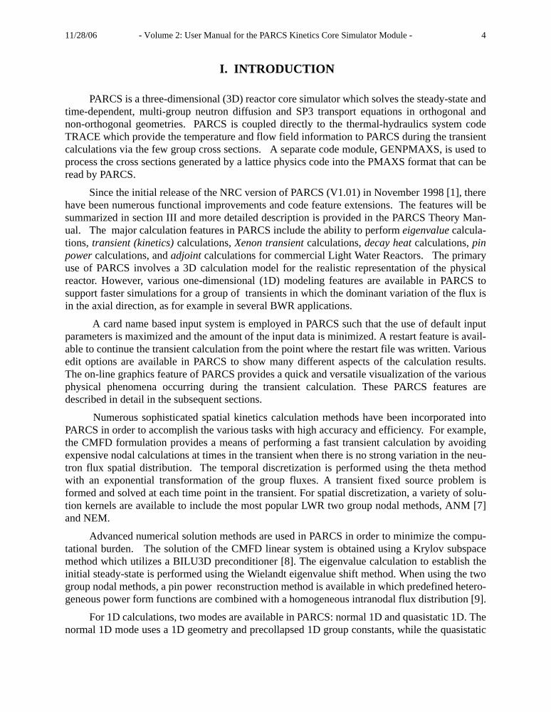
For the execution on a PC running the Windows operating system, a graphical user interfaceis available in PARCS. The first dialogue panel appears as in Figure 1.

11/28/06 - Volume 2: User Manual for the PARCS Kinetics Core Simulator Module - 13
Figure 1. PARCS User Input Interface
This panel displays the default input file name, parcs.inp. The user can choose a different inputfile name in the first window. Alternatively, if the user specifies a file name on the command linewhen executing PARCS(e.g. version 1.17 shown in figure 1), this name will appear in the firstpanel in place of parcs.inp. If the View_Selected_Options is clicked after the name of the inputfile and the working directory is specified, the contents of the input file is first read and theoptions specified in the input file will be reflected on the panel. For example, the External T/Hcheckbox will be selected if the EXT_TH card is set true in the CNTL block. Before executing thecode, the user can override what’s specified by the input file. Namely, one can change the caseidor the restart block number. Clicking the Go button after changes initiates the execution.
II.D Output Features
The PARCS output edits were designed to achieve the following four goals: 1) provide anecho and interpreter of all major input data of the code, 2) provide detailed information on variousphysical phenomena which occur during the transient, 3) provide a separate summary edit file at
11/28/06 - Volume 2: User Manual for the PARCS Kinetics Core Simulator Module - 14
the end of the run which contains essential information in a compact form, and 4) provide on-lineplotting of key parameters such as reactivity and core power to show the progress of the calcula-tion. PARCS generates various output files for later use, e.g. the restart file and the 1D cross sec-tion files. In the following, detailed PARCS output features are described.
II.D.1 Primary Output and Summary File
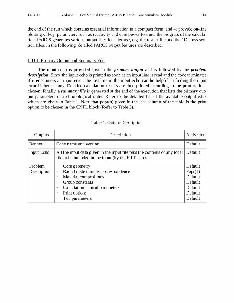
The input echo is provided first in the primary output and is followed by the problemdescription. Since the input echo is printed as soon as an input line is read and the code terminatesif it encounters an input error, the last line in the input echo can be helpful in finding the inputerror if there is any. Detailed calculation results are then printed according to the print optionschosen. Finally, a summary file is generated at the end of the execution that lists the primary out-put parameters in a chronological order. Refer to the detailed list of the available output editswhich are given in Table 1. Note that popt(n) given in the last column of the table is the printoption to be chosen in the CNTL block (Refer to Table 3).
Table 1. Output Description
Outputs Description Activation
Banner Code name and version Default
Input Echo All the input data given in the input file plus the contents of any local file to be included in the input (by the FILE cards)
Default
ProblemDescription
• Core geometry• Radial node number correspondence• Material compositions • Group constants• Calculation control parameters• Print options• T/H parameters
DefaultPopt(1)DefaultDefaultDefaultDefaultDefault

11/28/06 - Volume 2: User Manual for the PARCS Kinetics Core Simulator Module - 15
Steady-StateResults
• Iteration table.• keff, ppm, core power etc.• Axially averaged assembly power and pin power distribution• Axial power distribution• Planar assembly power and pin power distribution• Axial avg. assembly moderator temperature distribution• Axial avg. assembly outlet moderator temperature distribution• Axial moderator temperature distribution• Axial avg. assembly fuel temperature distribution • Axial fuel temperature distribution• Axial avg. assembly fuel centerline temperature distribution • Axial avg. assembly maximum fuel centerline temperature distri-
bution • Axial avg. assembly Xenon/Samarium number density distribuion • Planar Xenon/Samarium number density distribution
• Axially averaged assembly flux distribution• Axial flux distribution• Planar assembly flux distribution• Axial avg. assembly precursor density distribution• Collapsed 1-D cross section• Iteration table for adjoint flux calculation• Axial avg. assembly adjoint flux distribution
Popt(2)DefaultDefaultDefaultPopt(3)Popt(10)Popt(10)Popt(10)Popt(10)Popt(10)Popt(10)Popt(10)
XE_SMXE_SM+Popt(9)Popt(7)Popt(7)Popt(8)Popt(7)Popt(11)Popt(6)Popt(6)
Outputs Description Activation

11/28/06 - Volume 2: User Manual for the PARCS Kinetics Core Simulator Module - 16
II.D.2 Output Files
Table 2 shows the list of available output files. The three character file extension is attachedto the caseid specified in the input to form each file name. The pin power file contains detailed pin
TransientResults
(at each time step)
• Core state change which drives transient• Iteration table• Reactivity (in $) and core power(% total power)• Axially averaged assembly power and pin power distribution• Axial power distribution• Planar assembly power and pin power distribution• Axial avg. assembly moderator temperature distribution• Axial avg. assembly outlet moderator temperature distribuion• Axial moderator temperature distribution• Axial avg. assembly fuel temperature distribution • Axial fuel temperature distribution• Axial avg. assembly fuel centerline temperature distribution • Axial avg. assembly maximum fuel centerline temperature distri-
bution • Axial avg. assembly Xenon/Samarium number density distriuion • Planar Xenon/Samarium number density distribution
• Axial avg. assembly flux distribution• Axial flux distribution• Planar assembly flux distribution• Axial avg. assembly precursor density distribution
DefaultPopt(2)DefaultDefaultDefaultPopt(3)Popt(10)Popt(10)Popt(10)Popt(10)Popt(10)Popt(10)Popt(10)
XE_SMXE_SM+Popt(9)Popt(7)Popt(7)Popt(8)Popt(7)
Summary Edits
(for all time points)
• Overall Summary with the time step - Reactivity (in $) - Power level (% of maximum rated power) - Fxy (box relative power and pin relative power) - Fq - Maximum and average coolant temperature ( )
- Maximum and average fuel temperature( )• Axial avg. assembly power density summary - Assembly power - Fxy - Fq• Axial power shape• Axial avg. assembly flux distribution• Axial flux shape
Default
Default
DefaultPopt(7)Popt(7)
Outputs Description Activation
°C
°K

11/28/06 - Volume 2: User Manual for the PARCS Kinetics Core Simulator Module - 17
power information for the assemblies for which the pin power calculation is requested. Thedetailed pin power option is turned on by POPT(4) of the PRINT_OPT card in the CNTL block.The restart file contains the restart information for each block. The frequency of the restart filewriting is determined by the RST_FREQ card in the TRAN block. A proper block numbershould be specified in the RESTART card in the CNTL block in a restart calculation. The globalparameter plot file contains global parameter changes vs. time. Core power and reactivity, maxi-mum fuel center-line temperature, and average outlet temperature are written here at each timestep. The file is always created in any transient calculation. The radial power/flux shape file con-tains the shape information needed for the QS1D or normal 1D calculation. The file writing isactivated by either POPT(13) for the power shape or POPT(14) for the flux shape in thePRINT_OPT card. The reactivity file contains various reactivity components such as Doppler orcontrol rod separated from the total reactivity. The reactivity components provide informationuseful in understanding the relative importance of various physical phenomena occurring duringthe transient. The component reactivity edit is activated by POPT(6) in the PRINT_OPT card.The XMGR plot file can be used to show the final plot off-line. This file is written on UNIX if thePLOT_CNTL card in the TRAN block is activated. The point kinetics data and 1D group con-stant files are to generate input parameters for lower dimensional models. The file creation is acti-vated by POPT(11) and POPT(12) for the 1D and Point Kinetics, respectively. The T/H feedbackvariable file is used to store the feedback related T/H variables at the specified calculated state.The Doppler temperatures and coolant temperatures and densities for each node are written tothis file. This file can be used later to combine various T/H conditions to generate 1D cross sec-tion at those states. The file creation is activated by the WRITE_FBV card in the TH block andthe file can be read by the READ_DOPL and READ_TMDM cards.
Table 2. PARCS Output Files
II.D.3 On-Line Graphics
One of the distinctive features of the new output system is the on-line plotting feature whichis based on XMGR graphics software for the UNIX application and the QuickWin graphics pack-age for the Windows application. Some of the primary transient calculation results such as reac-
Extension Description Extension Description
out Primary Output rho Feedback Component Reactivity
sum Summary Output ace XMGR Plot Window
pin Pin Power Output pkd Point Kinetics Data
rst Output Restart 1dx 1D Collapsed Group Constants
plt Global Parameter Plot Data dbg Debug output
shp Radial Power/Flux Shape fbv T/H Feedback variables

11/28/06 - Volume 2: User Manual for the PARCS Kinetics Core Simulator Module - 18
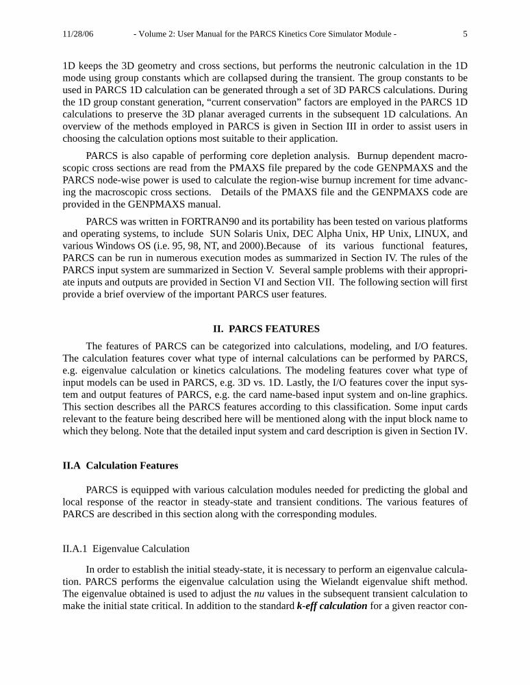
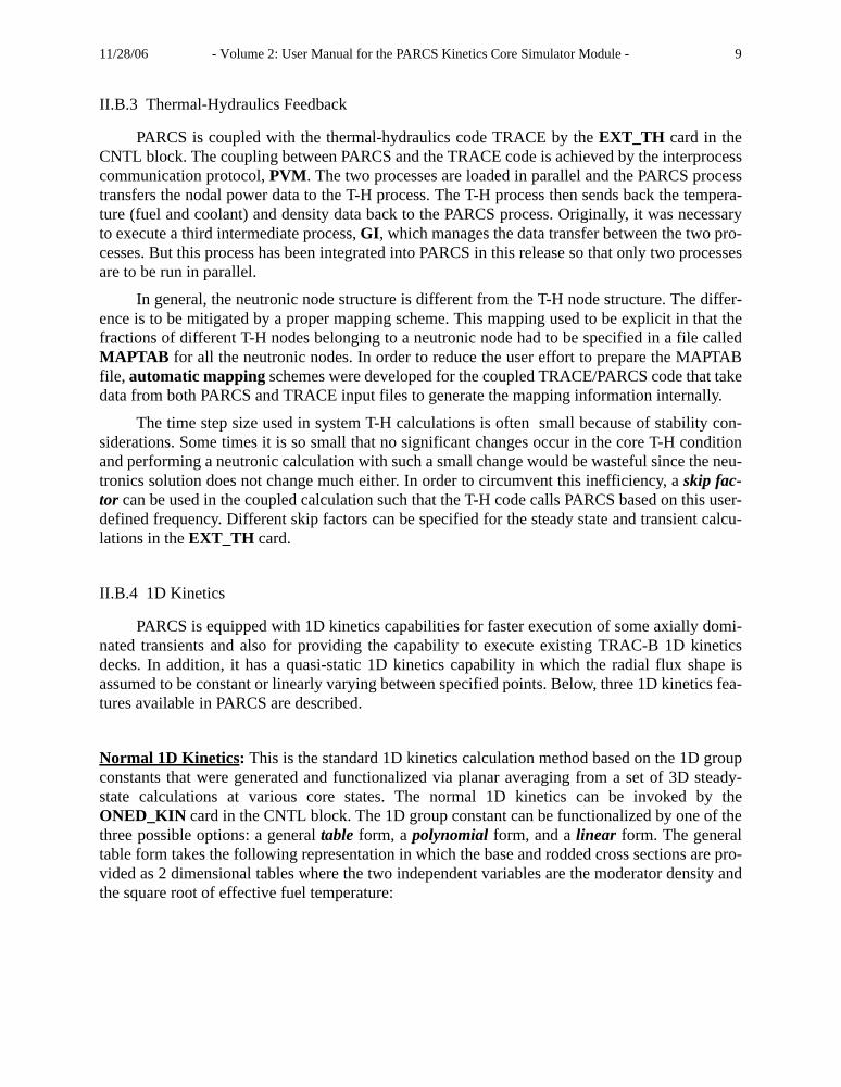
tivity, core power, peaking factors, and coolant and fuel temperatures are displayed on-line as thecalculation proceeds. The XMGR based on-line plot option can be chosen by the PLOT_CNTLcard in the TRAN block for the XMGR graphics. Figure 2 shows a sample on-line plot obtainedfor an analysis of a MSLB problem. As shown in Figure 3, the QuickWin based graphics providemore extensive and detailed on-line plots based on the directions given in the PLOT block.
QuickWin Based On-Line Graphics: The PARCS QuickWin (QW) on-line graphics utilizes theplotting kernels that were developed by a KAERI engineer, Dr. B. D. Chung. Permission to usethose kernels in PARCS was graciously given by him. There are three types of plots available inthe PARCS QW graphics: X-Y plot, axial distribution plot, and radial map. The variables thatcan be plotted are either global such as core power and reactivity or local such as relative nodalpower or effective fuel temperature. The local variables can be chosen from a group of PARCSsolution variable arrays by designating the location. The location is specified by a 5 digit numberin the form of kklll where kk designate the plane number while lll does the radial node index. Thevalue of zero for kk or lll invokes axially averaged or planar averaged values, respectively. Theplotable arrays are relative nodal power (relp), fast and thermal neutron fluxes (flux1 and flux2),coolant temperature (tcool), coolant density (dcool), fuel temperature (tfuel), fuel loading pattern(lp2d), and control rod positions (crpmap).
The X-Y plot is to display a global or a local quantity as a function of time. The globalparameters that can be plotted are k-eff, core power level, reactivity, average outlet coolant tem-perature, component reactivities, peaking factor, and control bank positions. Any local parameterscan be plotted with the spatial position specified by kklll. Several curves can be put in one X-Ygraph and a maximum of 50 X-Y plots can be put in one window. The choice of the X-axis type ismade by the XTYPE card in the PLOT block. The default x-axis variable is time and its maxi-mum is set by the tend given in the TIME_STEP card in the TRAN block. The XY card in thePLOT block selects the variables to be plotted and their minimum and maximum values.
The axial power distribution plot is to display the axial profile of a local quantity or a planaraveraged quantity. Core average axial power shapes, temperature, void profiles and many moreaxial plots can be made. The axial plot is controlled by the AXPLOT card in the PLOT block.
The radial map shows the radial distribution of local quantities at a selected plane or axially-averaged values. Radial power maps and temperature distributions can be plotted. There are threetypes of maps available: rectangular maps, contour maps, and filled contour maps. The rectangu-lar map shows colored boxes whose size is the same as a node. The contour and filled color mapsdraw contour line without and with color filling in between. The radial map is chosen and con-trolled by the RECTMAP, CONTOUR, and BITMAP cards in the PLOT block. The radial mapsare relatively complicated and thus take more computing time than the other plots. To alleviate theradial plotting overhead, the radial maps can be plotted infrequently by using the plot frequencyadjustment factor.

11/28/06 - Volume 2: User Manual for the PARCS Kinetics Core Simulator Module - 19
Figure 2. XMGR Based On-Line Plot Obtained During a MSLB Transient Calculation
0 20 40 60 80 100Time, sec
-7
-4.6
-2.2
0.2
2.6
5
rho,
$
Reactivity
TotalDopplerDensityCR
0 20 40 60 80 100Time, sec
0
24
48
72
96
120
Pow
er, %
Core Power
0 20 40 60 80 100Time, sec
1
3
5
7
9
11
Pea
king
Fac
tor
Peaking Factor
Fr-BoxFr-PinFq-Pin
0 20 40 60 80 100Time, sec
240
308
376
444
512
580
Tem
pera
ture
, C
Temperature
ToutTavgTfclTfuel

11/28/06 - Volume 2: User Manual for the PARCS Kinetics Core Simulator Module - 20
Figure 3. QuickWin Based On-Line Plot Obtained During a MSLB Transient Calculation
11/28/06 - Volume 2: User Manual for the PARCS Kinetics Core Simulator Module - 21
III. METHODS OVERVIEW
There is a separate volume in the TRACE theory manual that provides details of thePARCS spatial kinetics solution methods. It covers in detail the various methods used in PARCS,to include the spatial and temporal discretization methods, as well as several auxiliary calcula-tions that are required as part of standard reactor analysis. The detailed method description isessential to understanding the code’s capability and structure. However, most users may not needa detailed understanding of the method, and a brief explanation of the methods relevant to the exe-cution control are sufficient for the efficient use of the code. In the following subsections, theessential aspects of the PARCS calculation methods that are directly related to execution controlare explained so that the user can choose proper options to best suit their needs. Note that there aredefault parameters internally set in the code for the execution control inputs described below sothat it is not necessary to specifiy all parameters in the input.
III.A Spatial Discretization Methods
The spatial solution of the neutron flux in the reactor is determined in PARCS using wellestablished numerical methods. This section provides a brief overview of the essential methodsused in PARCS, to include theCMFD linear system formulation, the nodal methods available ineach geometry as well as the accompanying pin power reconstruction methods, the Krylov CMFDsolver, iteration control, and a special 1D kinetics method.
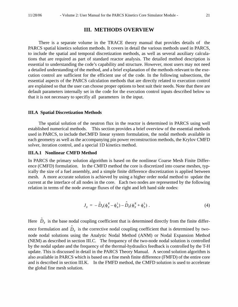
III.A.1 Nonlinear CMFD Method
In PARCS the primary solution algorithm is based on the nonlinear Coarse Mesh Finite Differ-ence (CMFD) formulation. In the CMFD method the core is discretized into coarse meshes, typ-ically the size of a fuel assembly, and a simple finite difference discretization is applied betweenmesh. A more accurate solution is achieved by using a higher order nodal method to update thecurrent at the interface of all nodes in the core. Each two nodes are represented by the followingrelation in terms of the node average fluxes of the right and left hand side nodes:
. (4)
Here is the base nodal coupling coefficient that is determined directly from the finite differ-
ence formulation and is the corrective nodal coupling coefficient that is determined by two-node nodal solutions using the Analytic Nodal Method (ANM) or Nodal Expansion Method(NEM) as described in section III.C. The frequency of the two-node nodal solution is controlledby the nodal update and the frequency of the thermal-hydraulics feedback is controlled by the T-Hupdate. This is discussed in detail in the PARCS Theory Manual. A second solution algorithm isalso available in PARCS which is based on a fine mesh finite difference (FMFD) of the entire coreand is described in section III.K. In the FMFD method, the CMFD solution is used to acceleratethe global fine mesh solution.
Jg D̃g φgR φg
L–( )– D̂g φgR φg
L+( )–=
D̃g
D̂g

11/28/06 - Volume 2: User Manual for the PARCS Kinetics Core Simulator Module - 22
In the initial eigenvalue calculation of the nonlinear CMFD method, the nodal update is per-formed with a specified fixed update frequency during the outer iteration. The default update fre-quency is 3 so that a nodal update is performed every three outer iterations. A different nodalupdate frequency can be chosen by the NLUPD_SS card in the PARAM block. The T-H update inthe steady-state is performed with a frequency based on the nodal update. Namely, the T-H updateis performed once per every n nodal updates. The default value of n is one meaning that the T-Hupdate is synchronized with the nodal update, but a different value can be selected by theNLUPD_SS card. There is an additional control parameter in the T-H update for the change in thefuel temperature. If the change is sufficiently small, namely the relative change is less than epstfin the CONV_SS card in the PARAM block, between the two successive T-H calculations, the T-H calculation is considered converged and no more T-H updates are made afterwards.
In the transient calculation as well as in the coupled steady-state calculation, the nodalupdate is only employed when there is a substantial change in the nodal cross sections. This is theconditional nodal update scheme. PARCS monitors the relative change in the total cross sectionat every node and invokes a nodal update when the change becomes larger than the value speci-fied in the EPS_XSEC card in the TRAN block (or epstf in the coupled steady-state calculation).The default value of epsxsec is 0.01. Choosing a smaller value causes more frequent nodalupdates making the solution more accurate but with more computing time, and vice versa. Once itis decided that the nodal update must be performed for the current time step, the invoking of theactual nodal update during the iteration to solve the transient fixed source problem is controlledby the update frequency and also by the error reduction ratio. By the use of the error reductionratio a nodal update can be invoked in a fewer number of iterations than the fixed number of iter-ations specified by the update frequency. The EPS_ERF and NLUPD_TR cards in the TRANblock specify the error reduction criterion and the fixed nodal update frequency.
The convergence of the iterative CMFD solution is checked with different criteria in theeigenvalue and transient calculations. In the eigenvalue calculation, the convergence of the k-eff,the local fission source (infinite norm), and the global fission source (2-norm) are checked againstthe convergence criteria specified in the CONV_SS card in the PARAM block by comparing twosuccessive iterates. This is consistent with convergence algorithms used in other codes. However,in the transient calculations, PARCS employs a unique convergence checking criterion by evalu-ating the relative residual. Since a fixed source problem of type Ax=b is solved in the transientproblem with a fixed right hand side vector b, the relative residual defined by
(5)
can be used as a measure of convergence without the need for comparing two successive iterates.Since PARCS employs the BiCGSTAB algorithm to solve the CMFD linear system and the resid-ual (the numerator in Eq. (5)) is computed as a by-product during the iteration, the relative resid-ual is obtained easily. The relative residual is compared against epsr2 specified in the CONV_TRcard in the TRAN block.
ςib Axi– 2
b 2-----------------------=

11/28/06 - Volume 2: User Manual for the PARCS Kinetics Core Simulator Module - 23
III.A. 2 Nodal Method
Nodal methods are the primary means used in PARCS to obtain higher order solutions to theneutron diffusion equation. Within the framework of the CMFD formulation the nodal method isused to solve the two node problem and to update the nodal coupling coefficient, , in Eq. (4).The ANM (Analytic Nodal Method) in PARCS has been used most frequently within the LightWater Reactor (LWR) industry to solve the two group diffusion equation. However, methodswere added to PARCS in order to address the so-called critical node problem, which can occurwhen there is no net leakage out of a node and the ANM matrix becomes singular [7] (also seePARCS Theory Manual). A second nodal method, the Nodal Expansion Method (NEM), wasadded which does not have this potential problem, but is less accurate for certain types of prob-lems [7]. A hybrid ANM-NEM method can then be used in which the ANM two-node problem isreplaced by a Nodal Expansion Method (NEM) two-node problem for the near critical nodes [7].In the hybrid method the user specifies a tolerance on the difference in the node k-inf and k-effwhich is used to switch between the ANM and NEM kernels (see PARAM card EPS_ANM).NEM is also available in a multi-group form for both cartesian and hexagonal geometries. Thefine mesh finite difference kernel (FMFD) has also been added to PARCS to provide pin by pinand higher order solution and is described in section III.K.
III.A.3 Pin Power Reconstruction
When using the nodal option in PARCS, it is necessary to invoke the pin power reconstruc-tion module in order to recover fuel pin powers from the nodal solution. Once the nodal fluxsolution is converged, the surface average currents are all determined. PARCS uses only the cur-rents to obtain intranodal flux distributions when the pin power option is selected. The homoge-neous flux solution is based on the analytic solution of a two dimensional fixed source problemhaving 8 boundary conditions among which 4 come from the 4 surface current and the other 4come from the 4 corner point fluxes. The axial transverse leakage and the transient fixed sourcewhich are included in the fixed source are represented by a 2 dimensional quadratic polynomial.Since the corner point fluxes are required, they are solved for first by using the corner point bal-ance relations(CPB) which couple all the corner point fluxes at a plane. During the formulation ofthe CPB equations, the corner point discontinuity factors (CDF) can be used to enhance the accu-racy. The coupled corner point flux linear system is solved by the Gauss-Seidel scheme. Once thecorner point fluxes are determined, the homogeneous intranodal fluxes can be obtained indepen-dently for each node. The homogeneous flux is then multiplied by the power form functionswhich are provided for each energy group, typically from a separate lattice calculation. The use ofthe analytic solution form employing only currents, CDF, and the two group power form functionsprovide superior accuracies in the pin power calculation as demonstrated in Reference [2]. Notethat the ordinary one group power form functions can be used by specifying only the first groupvalues in the PFF block.
III.A.4 Control Rod Cusping Correction
When a node is partially rodded, there appears a so called control rod cusping effect if thecontrol rod cross section is incorporated using the volume fraction only. This occurs inherently
D̂g
11/28/06 - Volume 2: User Manual for the PARCS Kinetics Core Simulator Module - 24
because there is a flux depression in the partially rodded region leading to a smaller control rodworth. The rod cusping problem is addressed in PARCS by solving a three node problem using afine mesh finite difference method (FDM). The three nodes include the upper and lower nodes aswell as the partially rodded node. The node average fluxes of the upper and lower nodes are usedas constraints. The solution of the three node problem is the intranodal flux and this is used tocompute the flux depression factor. The first decusping option uses only this flux depression fac-tor while there is another option to define axial discontinuity factors from the three node problemfor use in the subsequent two-node problems. The first decusping option is sufficiently accurateand must be used in a transient where the control rods are slowly moving or many nodes are par-tially rodded. It is specified by the DECUSP card in the PARAM block.
III.A.5 1D Nodal Kinetics
The 1D solver uses the same calculation models employed in the 3D PARCS solution tomaintain consistency with the 3D module. Namely, the basic solution method for the 1D kineticsequation is the nonlinear analytic nodal method (ANM) and the theta temporal discretization. Dueto the use of ANM, the axial node size of the 1D module can be chosen as large as 20-30 cm,yielding only 12 to 25 axial nodes. Also the newly derived current conservation factor (CCF) isintroduced which guarantees the same axial currents as the 3D reference values. By using theCCF factor, the 1D kinetics module can reproduce the 3D axial power distribution. This enhancesthe accuracy and makes it possible to generate the same initial condition as the 3D solution. Thesolution of the 1D kinetics equation involves a block tridiagonal linear system that is solveddirectly by using the direct elimination method.
The additional functions of the 1D kinetics module include various 1D cross section repre-sentation schemes and multi-channel treatment by using an input specifying radial weighting fac-tors for the corresponding external T/H calculation. In the 1D module, three 1D cross sectionforms are allowed: the tabular, polynomial, and linear cross section representation schemes. Thetabular representation scheme on fuel temperature and moderator density provides a wide rangeof applicability and enhances the accuracy of the 1D kinetics solution. In addition, multiple con-trol bank modeling is possible and the control rod cusping problem is solved by using a quadraticdecusping function. The coefficients of the decusping function can be given for each control rodbank.
Most 1D routines were written in FORTRAN90 to take advantage of dynamic memory allo-cation and derived data types. The 1D module thus has different memory addresses even thoughthe same variable names are used as in the 3D routines. Due to the use of dynamic memory alloca-tion, no 1D memory will be allocated during the normal 3D runs so that the addition of the 1Droutine will not harm the execution of the 3D module.
The input/output (I/O) formats of the 1D module were made consistent with the 3D modulein order to minimize newly defined input cards and also to provide convenient user accessibility.When the 1D module is invoked, the input data necessary for the 1D module is transferred from3D common blocks to 1D common blocks. After that the 1D module is independently executed inthe normal calculation mode without triggering any 3D routines.

11/28/06 - Volume 2: User Manual for the PARCS Kinetics Core Simulator Module - 25
III.A.6 Hexagonal Geometry
The hexagonal core calculation method implemented in PARCS is basically the same non-linear CMFD formulation having a higher order hexagonal nodal coupling kernel which utilizesthe triangular polynomial expansion nodal (TPEN) method. Since the CMFD formulation is alsoused for the cartesian geometry options, the hexagonal and rectangular solvers in PARCS are con-sistent, in that they share the same problem control logic, driver routines, and variable structures.There are some notable differences between the two modules, such as the formulation of the nodalkernel. For example, the cartesian solvers use transverse-integrated nodal methods in which thethree-dimensional problem is decomposed into three one-dimensional problems. In the hexagonalmodule, the non-transverse-integrated method TPEN solves a two-dimensional problem directly,rather than solving two coupled one-dimensional problems in each plane as in the cartesian nodalmethod. In the TPEN method, the three-dimensional problem is first decoupled into a radial andan axial problem that are coupled through transverse-leakages. Radially, the two-dimensionalproblem for each hexagon is solved by first splitting the hexagon into six triangles and thenexpanding the two-dimensional intranodal flux solution for each triangle into a two-dimensionalthird order polynomial.
In order to solve the CMFD linear system for the hexagonal problem, the same Krylov sub-space algorithm (BiCGSTAB) used for the rectangular problems is employed for hexagonalgeometry, but with a simplified diagonal preconditioner. The primary reason for the choice of thediagonal preconditioner rather than the more effective BILU3D preconditioner for rectangularproblems was the difficulty of handling various symmetries. In the hexagonal geometry, 1/12, 1/6,1/3, and 1/2 core problems exists and the symmetry changes the structure of the CMFD matrix.Thus it is nontrivial to construct an incomplete LU factorization scheme that works generallyregardless of the symmetry option. On the contrary, the diagonal preconditioner can be easilyapplied to any type of matrix structure and was chosen here as the preconditioner for the hexago-nal problems.
The basic PARCS CMFD calculation logic developed for the rectangular geometry has beenretained in the hexagonal geometry solver. Namely, the calculation flow remains mostlyunchanged and only the preconditioned equation solver and the nodal kernel differ. For example,the Wielandt method, the temporal discretization scheme (the theta method with exponentialtransform), and the nonlinear nodal and T/H update logics are commonly used in both geometrysolvers.
III.A.7 FMFD Kernel
For some applications (e.g. MOX core analysis) the explicit representation of each fuel pinwithin the fuel assembly may be warranted and therefore a multigroup fine mesh finite difference(FMFD) kernel was added as another spatial discretization option in PARCS. A separate set ofinput cards (FMFD block) are required to run FMFD in which a pin-wise composition map isspecified for each unique assembly type. The FMFD block also includes cross sections andenergy group information, and therefore the standard XSEC block is not necessary when execut-ing in the fine mesh mode. Coarse mesh acceleration information is specified using the grid_x,
11/28/06 - Volume 2: User Manual for the PARCS Kinetics Core Simulator Module - 26
grid_y, neutmesh_x, and neutmesh_y cards. Fuel assembly-wise feedback is default but pin bypin thermal feedback can be applied by the GENINF card, meshth field. The FMFD kernel isavailable in both diffusion theory and SP3 transport, as described in the next section.
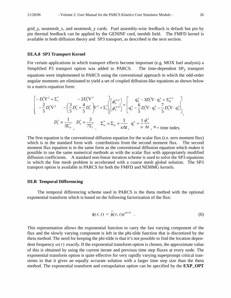
III.A.8 SP3 Transport Kernel
For certain applications in which transport effects become important (e.g. MOX fuel analysis) aSimplified P3 transport option was added to PARCS. The time-dependent SP3 transportequations were implemented in PARCS using the conventional approach in which the odd-orderangular moments are eliminated to yield a set of coupled diffusion-like equations as shown belowin a matrix-equation form:
,
, , , , = time index.
The first equation is the conventional diffusion equation for the scalar flux (i.e. zero moment flux)which is in the standard form with contributions from the second moment flux. The secondmoment flux equation is in the same form as the conventional diffusion equation which makes itpossible to use the same numerical methods as with the scalar flux with appropriately modifieddiffusion coefficients. A standard non-linear iteration scheme is used to solve the SP3 equationsin which the fine mesh problem is accelerated with a coarse mesh global solution. The SP3transport option is available in PARCS for both the FMFD and NEMMG kernels.
III.B Temporal Differencing
The temporal differencing scheme used in PARCS is the theta method with the optionalexponential transform which is based on the following factorization of the flux:
. (6)
This representation allows the exponential function to carry the fast varying component of theflux and the slowly varying component is left in the phi-tilde function that is discretized by thetheta method. The need for keeping the phi-tilde is that it’s not possible to find the location depen-dent frequency exactly. If the exponential transform option is chosen, the approximate valueof this is obtained by using the current iterate and previous time step fluxes at every node. Theexponential transform option is quite effective for very rapidly varying superprompt critical tran-sients in that it gives an equally accurate solution with a larger time step size than the thetamethod. The exponential transform and extrapolation option can be specified by the EXP_OPT
⎥⎥
⎦
⎤
⎢⎢
⎣
⎡
⋅∇−⋅∇−
+⋅∇−=⎥
⎦
⎤⎢⎣
⎡
⎥⎥⎥
⎦
⎤
⎢⎢⎢
⎣
⎡
Σ+∇⎟⎠⎞
⎜⎝⎛ +−∇−
∇−Σ+∇− +
+
+
nnn
nt
nn
n
n
t
r
qDqDq
SqDq
DDD
DD
3*31
*12
101
*10
12
10
*2*1
*3
2*1
2*1
*2*1
57
56
3
54
53
52
2
φφ
**1 3
1
tr
DΣ
≡ **3 7
3
t
DΣ
≡tΔ
+Σ=Συαα
1*
tq
nin
i Δ=
φυ1
n
φ r t,( ) φ̃ r t,( )ew r( )t=
ω r( )

11/28/06 - Volume 2: User Manual for the PARCS Kinetics Core Simulator Module - 27
card in the TRAN block while the theta value (default=0.5) can be adjusted for the fully implicitor explicit formulation in the THETA card in the TRAN block.
III.C Control Rod Scram Logic
The control rod scram logic in PARCS provides the user with the following control capabil-ities:
(1) Define a high flux trip set point(2) Define the delay from the time the trip is set to the time the rods begin to scram(3) Define the time to scram a rod from the “fully out” to the “fully in” position.(4) Define one or more “stuck rods”.
It should be noted that option (3) will be used to calculate a scram insertion rate, and that regard-less of the insertion position of any given rod, all control rods (except those define by option (4))will be inserted at this rate. The above logic input is implemented as follows:
- if power at time tn is greater than option (1), then set the trip and set tripbeg equal to tn- if the trip has been set and tn - tripbeg equals option(2), then set the scram and calculate
the insertion rate defined by option (3)
- if scram has been activated, insert all the rods (except those defined by option (4)) to theposition governed by option (3) and the time step size.
III.D Restart Capability
The restart capability in PARCS allows the user to define a frequency with which the restartdata should be written to file. This frequency is input as a multiple of the time step size. For exam-ple, if Δt=0.01, Tfinal=0.50, and the restart frequency is set to 10, then 5 restart edits will be per-formed which correspond to the following time steps: 0.1, 0.2, 0.3, 0.4, 0.5. This restart file canthen be utilized to begin another transient from any of the edit points in the existing file.
III.E Neutronic vs. T-H Variable Mapping
When T-H conditions for PARCS are provided by an external systems code (e.g. TRACE),the temperature/fluid condition required at each neutronics node for the feedback calculation con-sists of the coolant density/temperature and the effective fuel temperature. The nodal power infor-mation determined by PARCS is then transferred back to the systems code. During the course ofdata transfer, the difference in the neutronic and T-H nodalization are reconciled by the mappingscheme described below.
In general, coarser node sizes are used in the core T-H calculation than in the PARCS neu-tronics calculation. Therefore, a T-H node usually consists of several neutronics node. However, itis possible that a neutronics node can belong to multiple T-H nodes. Because of this possibility,

11/28/06 - Volume 2: User Manual for the PARCS Kinetics Core Simulator Module - 28
the PARCS T-H variable is obtained as the weighted average of the T-H variables of several T-Hnodes as:
(7)
where the superscript P and T stands for PARCS and T-H codes, and j(i,k) is the k-th T-H nodenumber out of the T-H nodes belonging to the i-th PARCS node. is the volume fraction ofthe j-th T-H node in the i-th PARCS node which must sum to unity.
On the other hand, the nodal power of the j-th T-H node is obtained as follows:
(8)
where i(j,k) is the k-th PARCS node number out of the PARCS nodes belonging to the j-th T-
H node. is the volume fraction of the i-th PARCS node in the j-th T-H node and satisfies thefollowing conditions:
. (9)
where is the number of all the T-H nodes. The second relation above implies that the T-Hnode larger than the PARCS nodes.
III.F Automatic TH/Neutronics Mapping
The General Interface (GI) code, which is the central interface unit between TRACE andPARCS, is included in the PARCS spatial kinetics code as a separate module. In this configura-tion, the PVM communication between PARCS and the GI has been replaced with direct datacopy logic, and the GI continues to manage all PVM communication with TRACE. Thus, twoprocesses (TRACE and PARCS) need to be executed.
In addition to this merging of the GI into PARCS, an automatic mapping kernel for the GIhas been designed and implemented. This kernel is currently able to manage the following map-ping configurations:
(1) Cylindrical T/H volumes from the TRACE vessel component to cartesian neutronicnodes, where no mapping information is specified. The weighting factors are com-puted based strictly on the geometric union of the cylindrical T/H grid and the carte-sian neutronic grid.
(2) Cylindrical T/H volumes from the TRACE vessel component to cartesian neutronicnodes, where a radial map is used to explicitly specify which radial T/H cell should becoupled to which neutronic node. Specifying this radial map allows the user to bypass
TiP αi j i k,( ),
P Tj i k,( )T
k 1=
NiP
∑=
NiP αi j,
P
PjT αj i j k,( ),
T Pi j k,( )P
k 1=
NjT
∑=
NjT
αj i,T
αj i,T
j 1=
NT
∑ 1 αj i j k,( ),T
k 1=
NjT
∑ 1>;=
NT
11/28/06 - Volume 2: User Manual for the PARCS Kinetics Core Simulator Module - 29
the mapping logic which computes weighting fractions based strictly on the geometricunion of the T/H and Neutronic grids.
(3) Multiple BWR CHAN components to a 3D neutronic core. This functionality requiresthat the user input a radial map which specifies the CHAN(s) to be coupled to eachneutronic node and with what weighting factor. It is the responsibility of the user toensure that the geometric volume of each T/H CHAN is consistent with the number ofneutronic nodes to which it is tied.
(4) BWR CHAN component(s) to a 1D neutronic core. This scenario arises from calcula-tions performed with either a TRAC-BF1 input deck (where PARCS processes the 1Dkinetics data from the TRAC-BF1 deck and thus does not need a separate PARCSinput deck or “MAPTAB” file), or a TRACE deck (where PARCS must process the 1Dkinetics data from its own input deck and a “MAPTAB” file is required).
The auto-mapping kernel works for calculations involving both old and new TRACE heatstructure formats, and no changes to the PARCS input deck or the “MAPTAB” file are required.The radial mapping for volumes and heat structures is performed based on one of the mappingconfigurations listed above, and the axial mapping is performed without user intervention. For theaxial mapping, a linear interpolation scheme is used for both the hydraulic cells and the heat struc-tures, which provides a fluid/fuel temperature distribution in the channel which is more accuratethan without interpolation. For the mapping of axial hydraulic cells, it is assumed that the fluidconditions exist at the exit of the cell.
The tabular weighting factors required in previous "MAPTAB" files are now no longer nec-essary. If this data is not input, or if only a radial map is specified, the code will assume that auto-matic mapping is to be performed. However, if this tabular data is present in the "MAPTAB" file,the auto-mapping logic will be deactivated, and the input weighting factors will be used. Sectiondescribes the input structure of the “MAPTAB” file in more detail.
Most 1D routines were written in FORTRAN90 to take advantage of dynamic memory allo-cation and derived data types. The 1D module thus has different memory addresses even thoughthe same variable names are used as in the 3D routines. Due to the use of dynamic memory alloca-tion, no 1D memory will be allocated during the normal 3D runs so that the addition of the 1Droutine will not harm the execution of the 3D module.
The input/output (I/O) formats of the 1D module were made consistent with the 3D modulein order to minimize newly defined input cards and also to provide convenient user accessibility.When the 1D module is invoked, the input data necessary for the 1D module is transferred from3D common blocks to 1D common blocks. After that the 1D module is independently executed inthe normal calculation mode without triggering any 3D routines.
III.G Core Depletion Analysis
The depletion capability was added to the PARCS code in version 2.5. A macroscopicdepletion module which adds the following functions to PARCS:
1) Ability to read in the macroscopic cross sections from PMAXS, the XS file prepared by theinterface code GENPXS

11/28/06 - Volume 2: User Manual for the PARCS Kinetics Core Simulator Module - 30
2) Ability to calculate region wise macroscopic cross sections as a function of the history state,such as burnup, moderate density history, control rod history
3) Ability to calculate region wise burnup increment at each step based on the region wise fluxes
The depletion module was implemented in PARCS by inserting several entry points in the code:
Figure 4. Schematic of implementation of DEPLETOR into PARCS
The depletion module is activated in PARCS using the input block DEPL which is described inthe user input. Utilization of the depletion option also requires the use of the two cards in theCNRL block and four cards in the TH block.
The burnup distribution is calculated using the fluxes provided by PARCS as follows:
where i : ith depletion region, one region is one Z-direction node of a assembly,
: burnup increase of i-th region,
: core average burnup increment in one step, specified in DEPLETOR input,
: the heavy metal loading in i-th region,
PREPROC
INPUTD
End
INIT
SSEIG
DEP_readinp
DEP_init: allocate variable prepare XS for initial state
DEP_main: Compute burnup & history prepare XS for current state
ΔBi ΔBcPiGc
PcGi-----------=
ΔBi
ΔBc
Gi

11/28/06 - Volume 2: User Manual for the PARCS Kinetics Core Simulator Module - 31
: total heavy metal loading in the core( ),
: power in i-th region,
: total power in core( )
, can be calculated as following :
,
,
where j : j-th neutronic node in PARCS,
g : g-th energy group,
: volume of j-th node, given by PARCS,
: heavy metal density in ith region, provided in PMAXS,
: fluxes, given by PARCS,
: fission energy XS, given by PARCS.
Gc Gi
i∑
Pi
Pc Pi
i∑
Gi Pi
Gi ρi Vj
j i∈∑=
Pi Vj κΣf g j, , φg j,
g∑
j i∈∑=
Vi
ρi
φg j,
κΣf g, ,

11/28/06 - Volume 2: User Manual for the PARCS Kinetics Core Simulator Module - 32
IV. EXECUTING PARCS
The various ways of executing PARCS are summarized in the following section. The spe-cific method of execution for each of the execution options is explained in the subsequent sec-tions.
IV.A Execution Modes
The execution modes of PARCS are categorized according to whether the calculation issteady state or transient, and 3D or 1D. Table 3 shows the execution mode classifications and thepossible calculation cases.
All of these calculation options are compatible with the exception of the eigenvalue search(1-1) and the critical boron search (1-2) for 3D steady-state calculations. Due to the nature of thecalculation for these options, they are mutually exclusive.
Table 3. Execution Modes of PARCS
Calculation Option Input Block Card Value
SteadyState
3D 1-1) Eigenvalue Search1-2) Critical Boron Search1-3) Adjoint Flux
CNTLCNTLCNTL
SEARCHSEARCH
PRINT_OPT
KEFF PPM
5
1D 2-1) Eigenvalue Search2-2) Adjoint Flux
CNTLCNTL
SEARCHPRINT_OPT
KEFF 5
Tran-sientCalcu-lation
3D 3-1) Control Rod Perturbation3-2) Boron Perturbation3-3) Scram3-4) Decay Heat3-5) Flow Perturbation
TRAN*TRAN*TRANCNTL
*
MOVE_BANKCHANGE_PPM
SCRAMDECAY_HEAT
1D 4-1) Control Rod Perturbation4-2) Boron Perturbation4-3) Scram without stuck rod4-4) Decay Heat4-5) Flow Perturbation
TRAN*TRAN*TRANCNTL
*
MOVE_BANKCHANGE_PPM
SCRAMDECAY_HEAT
* This option can be enabled through TRAC input as well.

11/28/06 - Volume 2: User Manual for the PARCS Kinetics Core Simulator Module - 33
IV.B PARCS Execution Procedure
This section explains the procedues to execute PARCS on a workstation and/or a PC for thevarious execution modes described above. Before executing PARCS, it should be compiled onthe target platform with the proper platform-dependent compiler directive (it should be noted thatthe Makefile included with the PARCS distribution should automatically define the necessarydirective). After the PARCS executable file has been compiled for the target platform, the usermust prepare the input file according to the card-name-based input description given in Section V.Most control input cards have default values, so the responsibility of the user is reduced to prepar-ing only the input cards necessary for solving the specific problem at hand.
For problems involving 1D and/or 3D steady state or transient problems, PARCS is run in acoupled mode with TRACE and PARCS run simultaneously. Figure 5 below outlines the proce-dure for performing a coupled analysis using TRACE and PARCS. The suggested procedure forcoupled calculations is as follows:
1. Run TRACE in the stand-alone mode for flow initialization (invoking no PARCS calcula-tions) and generate a restart file at the end of the run.
2. Using the above restart file, run the coupled steady state case and generate the steady staterestart files for both PARCS and TRACE. Adjust the external T-H skip factor so that exces-sive calls of PARCS are avoided. (Refer to the EXT_TH card in the CNTL block - nskipssparameter.)
3. Using the restart files, run the coupled transient case.
The first step can be omitted by starting the coupled run directly with the power ramp optiondefined (tdmrramp=1 in the TRACE namelist input). This option is valid only during steady-statecalculations.
The following steps are needed to actually perform each coupled run:
1. Open two windows on the screen.
2. Move to the TRACE run directory in one window.
3. Move to the PARCS run directory in another window. The maptab file described inSection III.F must exist in this directory, and the name of the file must be listed on theEXT_TH card of the PARCS CNTL block input.
4. Run TRACE.
5. Run PARCS by specifying the input file name as the argument, namely, parcs case.inp. Ifthe input file name is omitted, the default file name (parcs.inp) will be used.
When executing PARCS in the coupled 1D kinetics mode with a TRAC-B deck, no additionalPARCS input is necessary. However, the TRAC-B input file named tracin must exist in the work-ing directory. Running sequence is the same as the normal coupled run, but with no command lineargument (specifying the PARCS input file name).

11/28/06 - Volume 2: User Manual for the PARCS Kinetics Core Simulator Module - 34
Figure 5. Coupled TRACE/PARCS Execution Procedure Outline
XMGR(6)
Input Output
NOTES:
Input Output
TRACIN TRCMSGTRCOUTTRCDMPTRCXTVINLABTRCDIF
PARCS CODE
TRACCODE
Input Output
TRCMSGTRCOUTTRCDMPTRCXTVINLABTRCDIF
TRACCODE
TRACIN
TRCRST
Input Output
PARCS.INPMAPTAB
CASEID.SUMCASEID.OUTCASEID.PLTCASEID.RHOCASEID.RSTCASEID.PINCASEID.SHPCASEID.PKDCASEID.1DXCASEID.DBGCASEID.FBV
PARCS CODE
Input Output
PARCS.INPMAPTAB
CASEID.RST
CASEID.FBV
Menu Driven or Saved Files
Plots
(3) (4)
(5)
(7) (7)
Time EditsComponent Selection Variable Selection
TRANSIENTSTEADY STATET
RA
C-M
SU
PP
OR
T C
OD
ES
PA
RC
S(1) (2)
1. Usually requires one calculation.2. Usually requires a series of calculations of which only one is shown.3. Input-data file contains the full plant, steady-state description.4. A condensed version of the steady-state input-data file; all component descriptions are removed except those modified or added to initiate the transient calculation (e.g., breaks), and the possible addition of modified or new control-procedure parameters.5. Identical to the TRCDMP file from the previous calculation, except the file is renamed to satisfy the TRAC naming convention.6. X-Motif-based graphics post-processor.7. File TRCDIF contains diagnostic information that is used only by code developers (for null testing).8. Input data-file contains the full core, steady-state description.9. Input data-file contains the full-core, steady-state description with the addition of transient-inducing control procedures (e.g., control rod or boron perturbations).10. Input data-file contains the mapping between the thermal-hydraulic, heat structure, and neutronics nodalizations.11. Identical to the CASEID.RST file from the previous calculation, except the file is referenced in the transient PARCS.INP file.12. Optional input file used for generating point kinetics reactivity coefficients.13. Output files contain data sets directly readable by XMGR.14. Output files contain data sets easily extractable with user-generated, customized scripts.
(8) (9) CASEID.SUMCASEID.OUTCASEID.PLTCASEID.RHOCASEID.RSTCASEID.PINCASEID.SHPCASEID.PKDCASEID.1DXCASEID.DBGCASEID.FBV
(10) (10)
(11)
(12)
(14)
(13)

11/28/06 - Volume 2: User Manual for the PARCS Kinetics Core Simulator Module - 35
V. INPUT DESCRIPTION
V.A PARCS Input Card Description
Please refer to Section II.C for input guide lines and rules regarding the specific input cardsin this section. The first active (other than comments) input card should be the CASEID card thatprovides an alphanumeric case ID as the first field. The case ID is used to define the output filenames which are created by attaching the three character extensions (Refer to Table 2). Descrip-tive comments can be placed in the CASEID card. The input includes several blocks starting withthe CNTL block and ending with the TRAN block. PARAM, XSEC, GEOM, TH, PFF, PLOT,and ONEDK blocks are the blocks to appear in-between. The cards of each block are described inTables 4 through 13. Examples of each input card are shown with the syntax. If default values areto be used, the corresponding card can be omitted. It is recommended to use default parameters tomake the input compact.
Table 4. CNTL Cards
Card Type Field Default Description
CORE_TYPE alwropt PWR Core type: PWR = Pressurized Water Reactor BWR = Boiling Water ReactorCANDU = Pressurized Heavy Water ReactorPBR = Pebble Bed Reactor
CORE_TYPE BWR
CORE_POWER plevel 100.0 Initial core power level in %
CORE_POWER 70.000
PPM ppm 0.0 Initial boron concentration in ppm
PPM 1150.0
BANK_POS crbpos(1:ncrb) BIG Control rod bank position in steps withdrawn, ncrb is the number of control rod banks
BANK_POS 0.0 0.0 0.0 100.0 228.0 228.0 BANK_POS 3*0.0 100.0 2*228.0
TH_FDBK fdbk T T/H feedback option, either T(rue) or F(alse)Note: If Lths=T(rue) in INP_OPT card of DEPL block, the fdbk will be set to F(alse). See details in INP_OPT card of DEPL block.
TH_FDBK T

11/28/06 - Volume 2: User Manual for the PARCS Kinetics Core Simulator Module - 36
XE_SM ixesmopt 0 Xe/Sm option 0-No Xe/Sm 1-Equilibrium Xe/Sm 2-Transient Xe/Sm 3-user input Xe/Sm density 4-Equilibrium Xe/Sm at S.S. and Transient Xe/Sm during transient calculation
XE_SM 1
DECAY_HEAT decheat F Decay heat option, T or F
DECAY_HEAT T
SEARCH asrchopt None Criticality search option, KEFF, PPM
SEARCH KEFFSEARCH PPM
PIN_POWER pin F Pin power calculation option, T or F
PIN_POWER T
EXT_TH extth F External T/H option, T or F(Must be T for coupled TRAC/PARCS runs)Note: If Lths=T(rue) in INP_OPT card of DEPL block, the fdbk will be set to F(alse). See details in INP_OPT card of DEPL block.
afn MAPTAB File name of the Neutronics - T/H mapping table Refer to Section for detailed contents of the mapping table.
sysname TRAC System T-H Code TRAC for TRAC-E
nskipss 1 Steady-state external T-H skip factor (PARCS is called by the system code once per every nskipss time steps during the null transient cal-culation)
nskiptr 1 Transient external T-H skip factor
Table 4. CNTL Cards
Card Type Field Default Description

11/28/06 - Volume 2: User Manual for the PARCS Kinetics Core Simulator Module - 37
etf 0 Tolerance of Doppler temperature change rate (K/s) used to time advance coulpled calculation for depletion
rerr 0 Alternate method to control TH solution conver-gence during coupled steady-state calculation. When present, the product of Doppler tempera-ture change rate ‘etf’ and ‘rerr’ is used as the criteria of Doppler change rate used to initiate data exchange between PARCS and TH code.(note: This has not yet been implemented in TRAC-E)
Mthmatch 1 During steady-state calculation, maxium num-ber of TH steps before data exchange between PARCS and TH code (note: This has not yet been implemented in TRAC-E).
EXT_TH T MAPTAB TRAC 50 1 0.001 0.1 5
TRANSIENT tran F Transient calculation option, T or F
TRANSIENT T
RESTART rstrt F Restart option
afn None Input restart file, less than 80 characters long
irstbeg None Restart block number from which restart begins
RESTART T ssinit/ss.rst 2
Table 4. CNTL Cards
Card Type Field Default Description
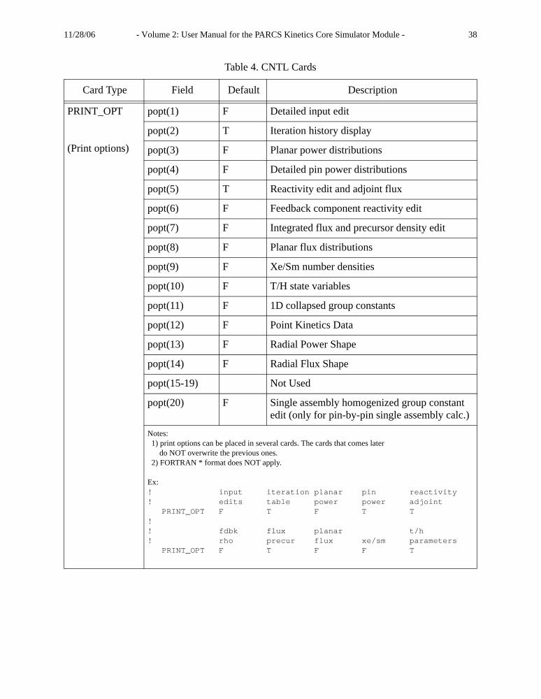
11/28/06 - Volume 2: User Manual for the PARCS Kinetics Core Simulator Module - 38
PRINT_OPT
(Print options)
popt(1) F Detailed input edit
popt(2) T Iteration history display
popt(3) F Planar power distributions
popt(4) F Detailed pin power distributions
popt(5) T Reactivity edit and adjoint flux
popt(6) F Feedback component reactivity edit
popt(7) F Integrated flux and precursor density edit
popt(8) F Planar flux distributions
popt(9) F Xe/Sm number densities
popt(10) F T/H state variables
popt(11) F 1D collapsed group constants
popt(12) F Point Kinetics Data
popt(13) F Radial Power Shape
popt(14) F Radial Flux Shape
popt(15-19) Not Used
popt(20) F Single assembly homogenized group constant edit (only for pin-by-pin single assembly calc.)
Notes: 1) print options can be placed in several cards. The cards that comes later do NOT overwrite the previous ones. 2) FORTRAN * format does NOT apply.
Ex:! input iteration planar pin reactivity ! edits table power power adjoint PRINT_OPT F T F T T !! fdbk flux planar t/h! rho precur flux xe/sm parameters PRINT_OPT F T F F T
Table 4. CNTL Cards
Card Type Field Default Description
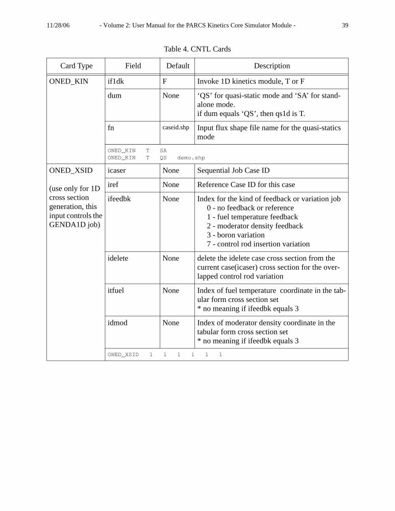
11/28/06 - Volume 2: User Manual for the PARCS Kinetics Core Simulator Module - 39
ONED_KIN if1dk F Invoke 1D kinetics module, T or F
dum None ‘QS’ for quasi-static mode and ‘SA’ for stand-alone mode.if dum equals ‘QS’, then qs1d is T.
fn caseid.shp Input flux shape file name for the quasi-statics mode
ONED_KIN T SAONED_KIN T QS demo.shp
ONED_XSID
(use only for 1D cross section generation, this input controls the GENDA1D job)
icaser None Sequential Job Case ID
iref None Reference Case ID for this case
ifeedbk None Index for the kind of feedback or variation job 0 - no feedback or reference 1 - fuel temperature feedback 2 - moderator density feedback 3 - boron variation 7 - control rod insertion variation
idelete None delete the idelete case cross section from the current case(icaser) cross section for the over-lapped control rod variation
itfuel None Index of fuel temperature coordinate in the tab-ular form cross section set* no meaning if ifeedbk equals 3
idmod None Index of moderator density coordinate in the tabular form cross section set* no meaning if ifeedbk equals 3
ONED_XSID 1 1 1 1 1 1
Table 4. CNTL Cards
Card Type Field Default Description
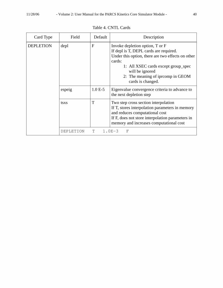
11/28/06 - Volume 2: User Manual for the PARCS Kinetics Core Simulator Module - 40
DEPLETION depl F Invoke depletion option, T or FIf depl is T, DEPL cards are required. Under this option, there are two effects on other cards: 1: All XSEC cards except group_spec will be ignored 2: The meaning of iprcomp in GEOM cards is changed.
espeig 1.0 E-5 Eigenvalue convergence criteria to advance to the next depletion step
tsxs T Two step cross section interpolationIf T, stores interpolation parameters in memory and reduces computational costIf F, does not store interpolation parameters in memory and increases computational cost
DEPLETION T 1.0E-3 F
Table 4. CNTL Cards
Card Type Field Default Description

11/28/06 - Volume 2: User Manual for the PARCS Kinetics Core Simulator Module - 41
XS_EXTRAP instrange 0 Cross section extrapolation range for instanta-neous variables. This range applies only to the branch type variable for each type of branch.
If the reference state value is higher than all the branch values, then the upper limit for the extrapolation is the reference + instrange*(refer-ence- maximum branch value) and the lower limit of the extrapolation is the reference -(1+instrange)* (reference- minimum branch value).
If the reference state value is lower than all branches values, then the upper limit for the extrapolation is the reference + (1+instrange)*( maximum branch value -reference) and the lower limit of the extrapolation is the reference - instrange* (reference- minimum branch value).
Otherwise, the upper limit of the extrapolation is the reference + (1+instrange)*(maximum branch value -reference) and the lower limit of the extrapolation is the reference -(1+instrange)* (reference- minimum branch value).
histrange instrange Cross section extrapolation range for history variables.
instpartr instrange Partial derivatives of cross section extrapolation range for instantaneous variables. This range applies to all variables. The lower limit will be (1+instpartr)*(minimum branch value) - instpartr*(second minimum branch value).The upper limit will be (1+instpartr)*(maximum branch value) - instpartr*(second maximum branch value).
histpartr histrange Partial derivatives of cross section extrapolation range for history variables.
XS_EXTRAP 1.0 0.3 0.8 0.2
Table 4. CNTL Cards
Card Type Field Default Description

11/28/06 - Volume 2: User Manual for the PARCS Kinetics Core Simulator Module - 42
ROT_ADF rotadf F Assembly rotation option, T or F
ROT_ADF T
DETECTOR detector F Detector response calculation, T or F
fnormd 1 Normalization factor for detector response
DETECTOR T 5.0E+6
Table 4. CNTL Cards
Card Type Field Default Description

11/28/06 - Volume 2: User Manual for the PARCS Kinetics Core Simulator Module - 43
TREE_XS Tree F Invoke tree structure XS module, T or FIf tree is T, the cross sections always provided by either a separate XESC file of depletion mod-ule. The tree structure cross section format is described in Purdue Macroscopic Cross Section Library Format
NSet None Number of XS sets. if DEPL is T, NSet should be the number of fule zones(burnup regions) plus the number of XS sets for reflector regions.
The following flags indicate use or not use of the value provided by the XS file. If the flag is ‘F’, then default values will be used. If the values from XS file are the same as the default values, the user may use ‘F’ to reduce the computational cost.
Ladf T Assembly discontinuity factor
Lxes T Microscopic cross section of Xe and SM, No default value
Lded F Direct energy deposition fraction,default value 0
Lj1f F J1 factor for minimal critical power ratio, default:1
Lchi F Fission spectrum, default X(1)=1
Lchd F Delay neutron fission spectrum, default Xd(i)=X(i)
Linv F Inverse velocity, no default value, must be ‘T’ for transient
Ldet F Detector response XS, no default
Lyld F yield values of I, XE, Pm, the default yield val-ues are:0.06386,0.00228,0.0113
Lcdf F Corner discontinuity factor, default 1
Lgff F Group wise power form function, default 1
Lbet F Beta, default:0.0002584,0.00152,0.0013908
Lamb F Lambda, default: 0.0128,0.0318,0.119,0.3181,1.4027,3.9286
Table 4. CNTL Cards
Card Type Field Default Description

11/28/06 - Volume 2: User Manual for the PARCS Kinetics Core Simulator Module - 44
Ldec F Decay heat beta and lambda, default:Beta: 2.35402E-02,1.89077E-02,1.39236E-02 6.90315E-03,3.56888E-03,3.31633E-03Lamb:1.05345E-01,8.37149E-03,5.20337E-04 4.73479E-05,3.28153E-06,1.17537E-11
TREE_XS T 1024 T T F F F F F F F F F F F F
CANDU_CONF ixzconf(1:nx, 1:nz)
nx*nz*0 CANDU control rod banks defined for each non-dummy region of the vertical configuration (xz plane), 0 means no bank defined
CANDU_CONF 0 0 0 0 0 0 0 0 0 0 0 0 0 0 0 0 0 0 0 0 0 0 0 0 0 0 0 0 0 0 0 0 0 0 0 0 0 0 0 0 0 0 0 0 0 0 0 0 0 0 0 0 0 0 0 0 0 0 0 0 0 0 0 0 0 0 0 0 0 0 0 0 0 0 0 0 0 0 0 0 0 0 0 0 0 0 0 0 0 0 0 0 0 0 0 0 0 0 0 0 0 0 0 0 0 1 1 0 0 0 0 0 0 0 0 2 2 0 0 0 0 0 0 0 0 4 4 0 0 0 0 0 0 0 0 0 0 0 1 1 0 0 0 0 0 0 0 0 2 2 0 0 0 0 0 0 0 0 4 4 0 0 0 0 0 0 0 0 0 0 0 0 0 0 0 0 0 0 0 0 0 0 0 0 0 0 0 0 0 0 0 0 0 0 0 0 0 0 0 0 0 0 0 0 0 0 0 0 0 0 0 0 0 0 0 0 0 0 0 0 0 0 0 0 0 0 0 0 0 0 0 0 0 0 0 0 0 3 3 0 0 0 0 0 0 0 0 5 5 0 0 0 0 0 0 0 0 1 1 0 0 0 0 0 0 0 0 0 0 0 3 3 0 0 0 0 0 0 0 0 5 5 0 0 0 0 0 0 0 0 1 1 0 0 0 0 0 0 0 0 0 0 0 0 0 0 0 0 0 0 0 0 0 0 0 0 0 0 0 0 0 0 0 0 0 0 0 0 0 0 0 0 0 0 0 0 0 0 0 0 0 0 0 0 0 0 0 0 0 0 0 0 0 0 0 0 0 0 0 0 0 0 0 0 0 0 0 0 0 2 2 0 0 0 0 0 0 0 0 1 1 0 0 0 0 0 0 0 0 6 6 0 0 0 0 0 0 0 0 0 0 0 2 2 0 0 0 0 0 0 0 0 1 1 0 0 0 0 0 0 0 0 6 6 0 0 0 0 0 0 0 0 0 0 0 0 0 0 0 0 0 0 0 0 0 0 0 0 0 0 0 0 0 0 0 0 0 0 0 0 0 0 0 0 0 0 0 0 0 0 0 0 0 0 0 0 0 0 0 0 0 0 0 0 0 0 0 0 0 0 0 0 0 0 0 0 0 0 0 0 0 0 0 0 0 0 0 0 0 0 0 0 0 0 0 0 0 0 0 0 0 0 0 0 0 0 0 0
Table 4. CNTL Cards
Card Type Field Default Description
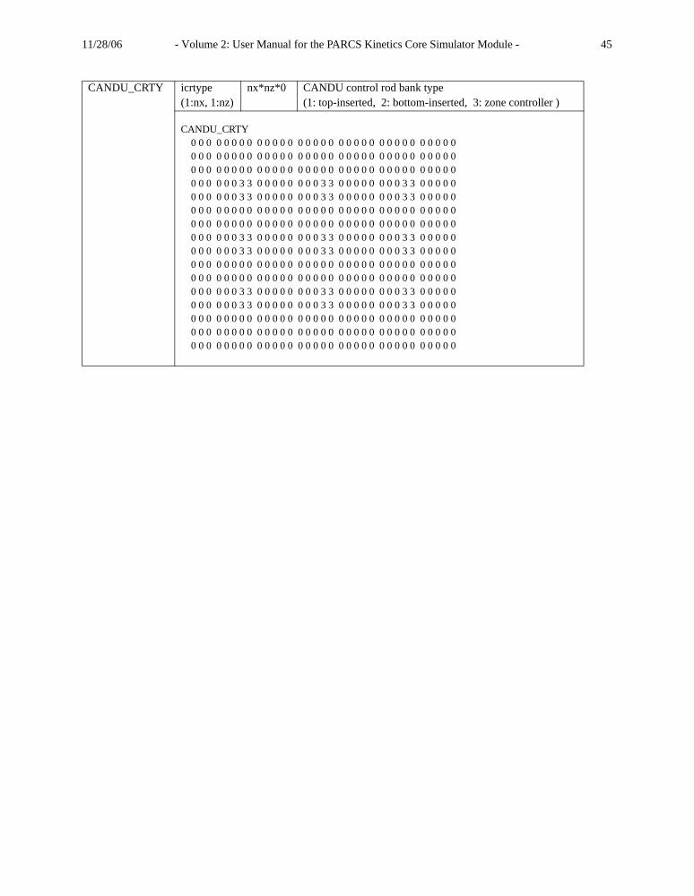
11/28/06 - Volume 2: User Manual for the PARCS Kinetics Core Simulator Module - 45
CANDU_CRTY icrtype(1:nx, 1:nz)
nx*nz*0 CANDU control rod bank type(1: top-inserted, 2: bottom-inserted, 3: zone controller )
CANDU_CRTY 0 0 0 0 0 0 0 0 0 0 0 0 0 0 0 0 0 0 0 0 0 0 0 0 0 0 0 0 0 0 0 0 0 0 0 0 0 0 0 0 0 0 0 0 0 0 0 0 0 0 0 0 0 0 0 0 0 0 0 0 0 0 0 0 0 0 0 0 0 0 0 0 0 0 0 0 0 0 0 0 0 0 0 0 0 0 0 0 0 0 0 0 0 0 0 0 0 0 0 0 0 0 0 0 0 3 3 0 0 0 0 0 0 0 0 3 3 0 0 0 0 0 0 0 0 3 3 0 0 0 0 0 0 0 0 0 0 0 3 3 0 0 0 0 0 0 0 0 3 3 0 0 0 0 0 0 0 0 3 3 0 0 0 0 0 0 0 0 0 0 0 0 0 0 0 0 0 0 0 0 0 0 0 0 0 0 0 0 0 0 0 0 0 0 0 0 0 0 0 0 0 0 0 0 0 0 0 0 0 0 0 0 0 0 0 0 0 0 0 0 0 0 0 0 0 0 0 0 0 0 0 0 0 0 0 0 0 3 3 0 0 0 0 0 0 0 0 3 3 0 0 0 0 0 0 0 0 3 3 0 0 0 0 0 0 0 0 0 0 0 3 3 0 0 0 0 0 0 0 0 3 3 0 0 0 0 0 0 0 0 3 3 0 0 0 0 0 0 0 0 0 0 0 0 0 0 0 0 0 0 0 0 0 0 0 0 0 0 0 0 0 0 0 0 0 0 0 0 0 0 0 0 0 0 0 0 0 0 0 0 0 0 0 0 0 0 0 0 0 0 0 0 0 0 0 0 0 0 0 0 0 0 0 0 0 0 0 0 0 3 3 0 0 0 0 0 0 0 0 3 3 0 0 0 0 0 0 0 0 3 3 0 0 0 0 0 0 0 0 0 0 0 3 3 0 0 0 0 0 0 0 0 3 3 0 0 0 0 0 0 0 0 3 3 0 0 0 0 0 0 0 0 0 0 0 0 0 0 0 0 0 0 0 0 0 0 0 0 0 0 0 0 0 0 0 0 0 0 0 0 0 0 0 0 0 0 0 0 0 0 0 0 0 0 0 0 0 0 0 0 0 0 0 0 0 0 0 0 0 0 0 0 0 0 0 0 0 0 0 0 0 0 0 0 0 0 0 0 0 0 0 0 0 0 0 0 0 0 0 0 0 0 0 0 0 0 0 0
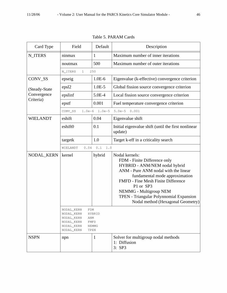
11/28/06 - Volume 2: User Manual for the PARCS Kinetics Core Simulator Module - 46
Table 5. PARAM Cards
Card Type Field Default Description
N_ITERS ninmax 1 Maximum number of inner iterations
noutmax 500 Maximum number of outer iterations
N_ITERS 1 250
CONV_SS
(Steady-State Convergence Criteria)
epseig 1.0E-6 Eigenvalue (k-effective) convergence criterion
epsl2 1.0E-5 Global fission source convergence criterion
epslinf 5.0E-4 Local fission source convergence criterion
epstf 0.001 Fuel temperature convergence criterion
CONV_SS 1.0e-6 1.0e-5 5.0e-5 0.001
WIELANDT eshift 0.04 Eigenvalue shift
eshift0 0.1 Initial eigenvalue shift (until the first nonlinear update)
targetk 1.0 Target k-eff in a criticality search
WIELANDT 0.04 0.1 1.0
NODAL_KERN kernel hybrid Nodal kernels: FDM - Finite Difference only HYBRID - ANM/NEM nodal hybrid ANM - Pure ANM nodal with the linear fundamental mode approximation FMFD - Fine Mesh Finite Difference P1 or SP3 NEMMG - Multigroup NEM TPEN - Triangular Polynnomial Expansion Nodal method (Hexagonal Geometry)
NODAL_KERN FDMNODAL_KERN HYBRIDNODAL_KERN ANMNODAL_KERN FMFDNODAL_KERN NEMMGNODAL_KERN TPEN
NSPN npn 1 Solver for multigroup nodal methods1: Diffusion3: SP3

11/28/06 - Volume 2: User Manual for the PARCS Kinetics Core Simulator Module - 47
NLUPD_SS nupdcy 3 Nonlinear update cycle (e.g. every 3 outers)
ninitout 3 Initial outers before the first nonlinear update
nmulth 1 Number of T/H updates per nodal update
NLUPD_SS 10 10 1
EPS_ANM epsanm 0.005 Near-criticality criterion needed for ANMstabilization
EPS_ANM 1.0e-06
EPS_ERF epserf 0.005 Error reduction criterion to exit inners
EPS_ERF 0.0005
DECUSP idecusp 0 Control rod cusping elimination option 0 - no decupsing 1 - flux shape correction only 2 - axial discontinuity as well (2 is not available in 1D kinetics module)
DECUSP 1
INIT_GUESS iguess 1 Initial guess for the axial flux shape 0 - cosine 1 - flat
INIT_GUESS 0
Table 6. XSEC Cards
Card Type Field Default Description
GROUP_SPEC mg 2 Number of Groups, If this card is present, the multigroup option, NEMMG, TPENMG is turned on even though the number of groups is 2.
mge(1) mg/2 The last fine group number belonging to the first group in the two-group structure.
GROUP_SPEC 2 1
Table 5. PARAM Cards
Card Type Field Default Description
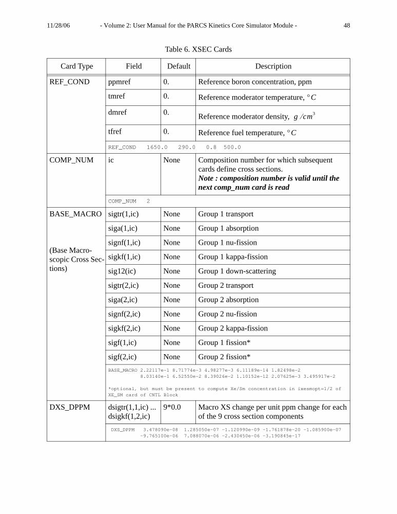
11/28/06 - Volume 2: User Manual for the PARCS Kinetics Core Simulator Module - 48
REF_COND ppmref 0. Reference boron concentration, ppm
tmref 0. Reference moderator temperature,
dmref 0. Reference moderator density,
tfref 0. Reference fuel temperature,
REF_COND 1650.0 290.0 0.8 500.0
COMP_NUM ic None Composition number for which subsequent cards define cross sections.Note : composition number is valid until the next comp_num card is read
COMP_NUM 2
BASE_MACRO
(Base Macro-scopic Cross Sec-tions)
sigtr(1,ic) None Group 1 transport
siga(1,ic) None Group 1 absorption
signf(1,ic) None Group 1 nu-fission
sigkf(1,ic) None Group 1 kappa-fission
sig12(ic) None Group 1 down-scattering
sigtr(2,ic) None Group 2 transport
siga(2,ic) None Group 2 absorption
signf(2,ic) None Group 2 nu-fission
sigkf(2,ic) None Group 2 kappa-fission
sigf(1,ic) None Group 1 fission*
sigf(2,ic) None Group 2 fission*BASE_MACRO 2.22117e-1 8.71774e-3 4.98277e-3 6.11189e-14 1.82498e-2 8.03140e-1 6.52550e-2 8.39026e-2 1.10152e-12 2.07625e-3 3.495917e-2
*optional, but must be present to compute Xe/Sm concentration in ixesmopt=1/2 of XE_SM card of CNTL Block
DXS_DPPM dsigtr(1,1,ic) ... dsigkf(1,2,ic)
9*0.0 Macro XS change per unit ppm change for each of the 9 cross section components
DXS_DPPM 3.478090e-08 1.285050e-07 -1.120990e-09 -1.761878e-20 -1.085900e-07 -9.765100e-06 7.088070e-06 -2.430450e-06 -3.190845e-17
Table 6. XSEC Cards
Card Type Field Default Description
°C
g cm3⁄
°C
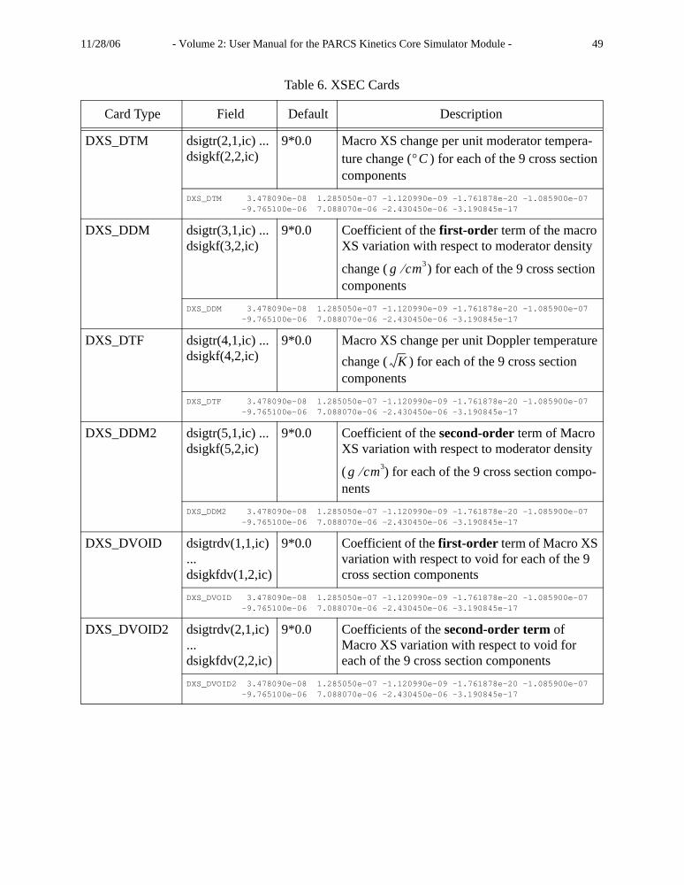
11/28/06 - Volume 2: User Manual for the PARCS Kinetics Core Simulator Module - 49
DXS_DTM dsigtr(2,1,ic) ... dsigkf(2,2,ic)
9*0.0 Macro XS change per unit moderator tempera-ture change ( ) for each of the 9 cross section components
DXS_DTM 3.478090e-08 1.285050e-07 -1.120990e-09 -1.761878e-20 -1.085900e-07 -9.765100e-06 7.088070e-06 -2.430450e-06 -3.190845e-17
DXS_DDM dsigtr(3,1,ic) ... dsigkf(3,2,ic)
9*0.0 Coefficient of the first-order term of the macro XS variation with respect to moderator density
change ( ) for each of the 9 cross section components
DXS_DDM 3.478090e-08 1.285050e-07 -1.120990e-09 -1.761878e-20 -1.085900e-07 -9.765100e-06 7.088070e-06 -2.430450e-06 -3.190845e-17
DXS_DTF dsigtr(4,1,ic) ... dsigkf(4,2,ic)
9*0.0 Macro XS change per unit Doppler temperature change ( ) for each of the 9 cross section components
DXS_DTF 3.478090e-08 1.285050e-07 -1.120990e-09 -1.761878e-20 -1.085900e-07 -9.765100e-06 7.088070e-06 -2.430450e-06 -3.190845e-17
DXS_DDM2 dsigtr(5,1,ic) ... dsigkf(5,2,ic)
9*0.0 Coefficient of the second-order term of Macro XS variation with respect to moderator density
( ) for each of the 9 cross section compo-nents
DXS_DDM2 3.478090e-08 1.285050e-07 -1.120990e-09 -1.761878e-20 -1.085900e-07 -9.765100e-06 7.088070e-06 -2.430450e-06 -3.190845e-17
DXS_DVOID dsigtrdv(1,1,ic) ...dsigkfdv(1,2,ic)
9*0.0 Coefficient of the first-order term of Macro XS variation with respect to void for each of the 9 cross section components
DXS_DVOID 3.478090e-08 1.285050e-07 -1.120990e-09 -1.761878e-20 -1.085900e-07 -9.765100e-06 7.088070e-06 -2.430450e-06 -3.190845e-17
DXS_DVOID2 dsigtrdv(2,1,ic) ... dsigkfdv(2,2,ic)
9*0.0 Coefficients of the second-order term of Macro XS variation with respect to void for each of the 9 cross section components
DXS_DVOID2 3.478090e-08 1.285050e-07 -1.120990e-09 -1.761878e-20 -1.085900e-07 -9.765100e-06 7.088070e-06 -2.430450e-06 -3.190845e-17
Table 6. XSEC Cards
Card Type Field Default Description
°C
g cm3⁄
K
g cm3⁄
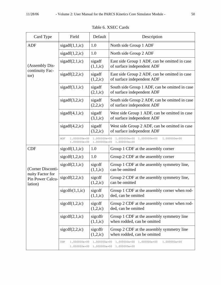
11/28/06 - Volume 2: User Manual for the PARCS Kinetics Core Simulator Module - 50
ADF
(Assembly Dis-continuity Fac-tor)
sigadf(1,1,ic) 1.0 North side Group 1 ADF
sigadf(1,2,ic) 1.0 North side Group 2 ADF
sigadf(2,1,ic) sigadf(1,1,ic)
East side Group 1 ADF, can be omitted in case of surface independent ADF
sigadf(2,2,ic) sigadf(1,2,ic)
East side Group 2 ADF, can be omitted in case of surface independent ADF
sigadf(3,1,ic) sigadf(2,1,ic)
South side Group 1 ADF, can be omitted in case of surface independent ADF
sigadf(3,2,ic) sigadf(2,2,ic)
South side Group 2 ADF, can be omitted in case of surface independent ADF
sigadf(4,1,ic) sigadf(3,1,ic)
West side Group 1 ADF, can be omitted in case of surface independent ADF
sigadf(4,2,ic) sigadf(3,2,ic)
West side Group 2 ADF, can be omitted in case of surface independent ADF
ADF 1.000000e+00 1.000000e+00 1.000000e+00 1.000000e+00 1.000000e+00 1.000000e+00 1.000000e+00 1.000000e+00
CDF
(Corner Disconti-nuity Factor for Pin Power Calcu-lation)
sigcdf(1,1,ic) 1.0 Group 1 CDF at the assembly corner
sigcdf(1,2,ic) 1.0 Group 2 CDF at the assembly corner
sigcdf(2,1,ic) sigcdf(1,1,ic)
Group 1 CDF at the assembly symmetry line, can be omitted
sigcdf(2,2,ic) sigcdf(1,2,ic)
Group 2 CDF at the assembly symmetry line, can be omitted
sigcdfr(1,1,ic) sigcdf(1,1,ic)
Group 1 CDF at the assembly corner when rod-ded, can be omitted
sigcdf(1,2,ic) sigcdf(1,2,ic)
Group 2 CDF at the assembly corner when rod-ded, can be omitted
sigcdf(2,1,ic) sigcdfr(1,1,ic)
Group 1 CDF at the assembly symmetry line when rodded, can be omitted
sigcdf(2,2,ic) sigcdfr(1,2,ic)
Group 2 CDF at the assembly symmetry line when rodded, can be omitted
CDF 1.000000e+00 1.000000e+00 1.000000e+00 1.000000e+00 1.000000e+00
1.000000e+00 1.000000e+00 1.000000e+00
Table 6. XSEC Cards
Card Type Field Default Description
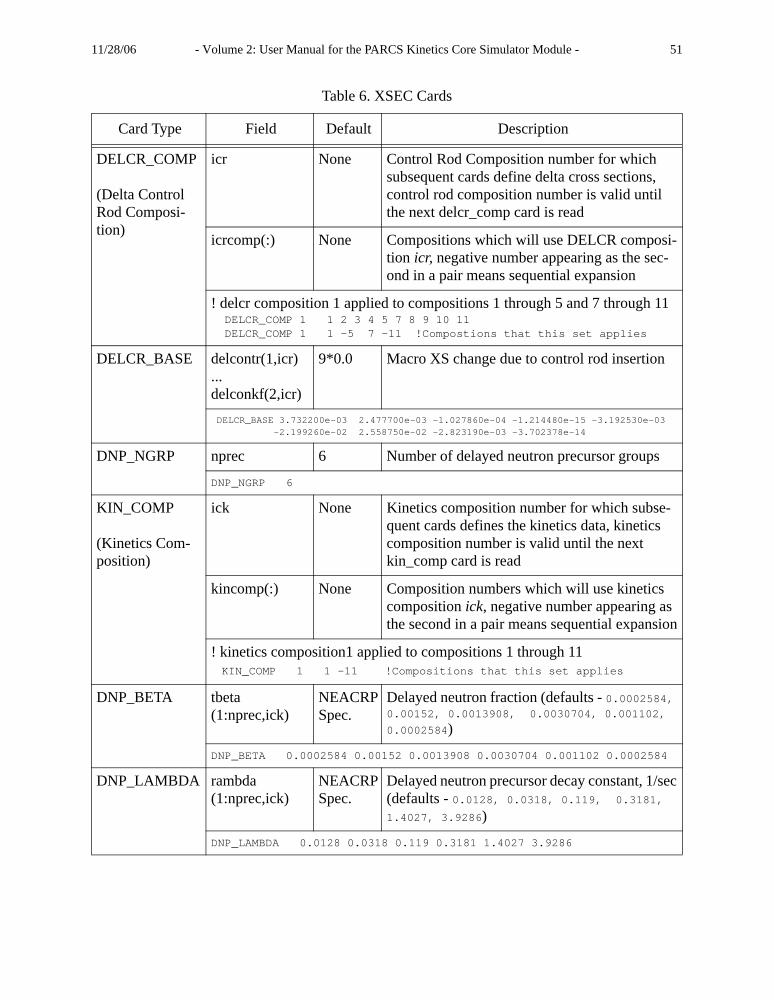
11/28/06 - Volume 2: User Manual for the PARCS Kinetics Core Simulator Module - 51
DELCR_COMP
(Delta Control Rod Composi-tion)
icr None Control Rod Composition number for which subsequent cards define delta cross sections, control rod composition number is valid until the next delcr_comp card is read
icrcomp(:) None Compositions which will use DELCR composi-tion icr, negative number appearing as the sec-ond in a pair means sequential expansion
! delcr composition 1 applied to compositions 1 through 5 and 7 through 11 DELCR_COMP 1 1 2 3 4 5 7 8 9 10 11 DELCR_COMP 1 1 -5 7 -11 !Compostions that this set applies
DELCR_BASE delcontr(1,icr) ... delconkf(2,icr)
9*0.0 Macro XS change due to control rod insertion
DELCR_BASE 3.732200e-03 2.477700e-03 -1.027860e-04 -1.214480e-15 -3.192530e-03 -2.199260e-02 2.558750e-02 -2.823190e-03 -3.702378e-14
DNP_NGRP nprec 6 Number of delayed neutron precursor groups
DNP_NGRP 6
KIN_COMP
(Kinetics Com-position)
ick None Kinetics composition number for which subse-quent cards defines the kinetics data, kinetics composition number is valid until the next kin_comp card is read
kincomp(:) None Composition numbers which will use kinetics composition ick, negative number appearing as the second in a pair means sequential expansion
! kinetics composition1 applied to compositions 1 through 11 KIN_COMP 1 1 -11 !Compositions that this set applies
DNP_BETA tbeta(1:nprec,ick)
NEACRP Spec.
Delayed neutron fraction (defaults - 0.0002584, 0.00152, 0.0013908, 0.0030704, 0.001102,
0.0002584)
DNP_BETA 0.0002584 0.00152 0.0013908 0.0030704 0.001102 0.0002584
DNP_LAMBDA rambda(1:nprec,ick)
NEACRP Spec.
Delayed neutron precursor decay constant, 1/sec (defaults - 0.0128, 0.0318, 0.119, 0.3181, 1.4027, 3.9286)
DNP_LAMBDA 0.0128 0.0318 0.119 0.3181 1.4027 3.9286
Table 6. XSEC Cards
Card Type Field Default Description

11/28/06 - Volume 2: User Manual for the PARCS Kinetics Core Simulator Module - 52
NEUT_VELO tvelo(1:2,ick) 2.8e74.4e5
Neutron velocity, cm/sec
NEUT_VELO 2.8e+07 4.4e+05
IXEPM_LAM rlambi 0.28750E-4 Decay constant of I
rlambxe 0.209167E-4 Decay constant of Xe
rlambpm 0.355568E-5 Decay constant of Pm
IXEPM_LAM 0.28750E-04 0.209167E-04 0.355568E-08
IXEPM_YLD gammafp(1,ic) 0.06386 Fission yield of I
gammafp(2,ic) 0.00228 Fission yield of Xe
gammafp(3,ic) 0.0113 Fission yield of Pm
IXEPM_YLD 0.06386 0.00228 0.0113
XESM_MICRO sigxea(1,ic) 1.05279E2 Group 1 Xe absorption micro xsec, barn
sigxea(2,ic) 1.45710E6 Group 2 Xe absorption micro xsec, barn
sigsma(1,ic) 9.07729E1 Group 1 Sm absorption micro xsec, barn
sigsma(2,ic) 5.52864E4 Group 2 Sm absorption micro xsec, barn
XESM_MICRO 1.05279E+02 1.45710E+06 9.07729E+01 5.52864E+04
DXESM_DPPM dsigxea(1,1,ic) 0. Group 1 Xe absorption micro xsec change per unit ppm change
dsigxea(1,2,ic) 0. Group 2 Xe absorption micro xsec change per unit ppm change
dsigsma(1,1,ic) 0. Group 1 Sm absorption micro xsec change per unit ppm change
dsigsma(1,2,ic) 0. Group 2 Sm absorption micro xsec change per unit ppm change
DXESM_DPPM 0.101 2.45E-01 0.99E-01 5.52
DXESM_DTM dsigxea(2,1,ic)...dsigsma(2,2,ic)
4*0. Xe and Sm absorption micro xsec change per unit moderator temperature change ( ) for each of the 4 micro components
DXESM_DTM 0.101 2.45E-01 0.99E-01 5.52
Table 6. XSEC Cards
Card Type Field Default Description
°C
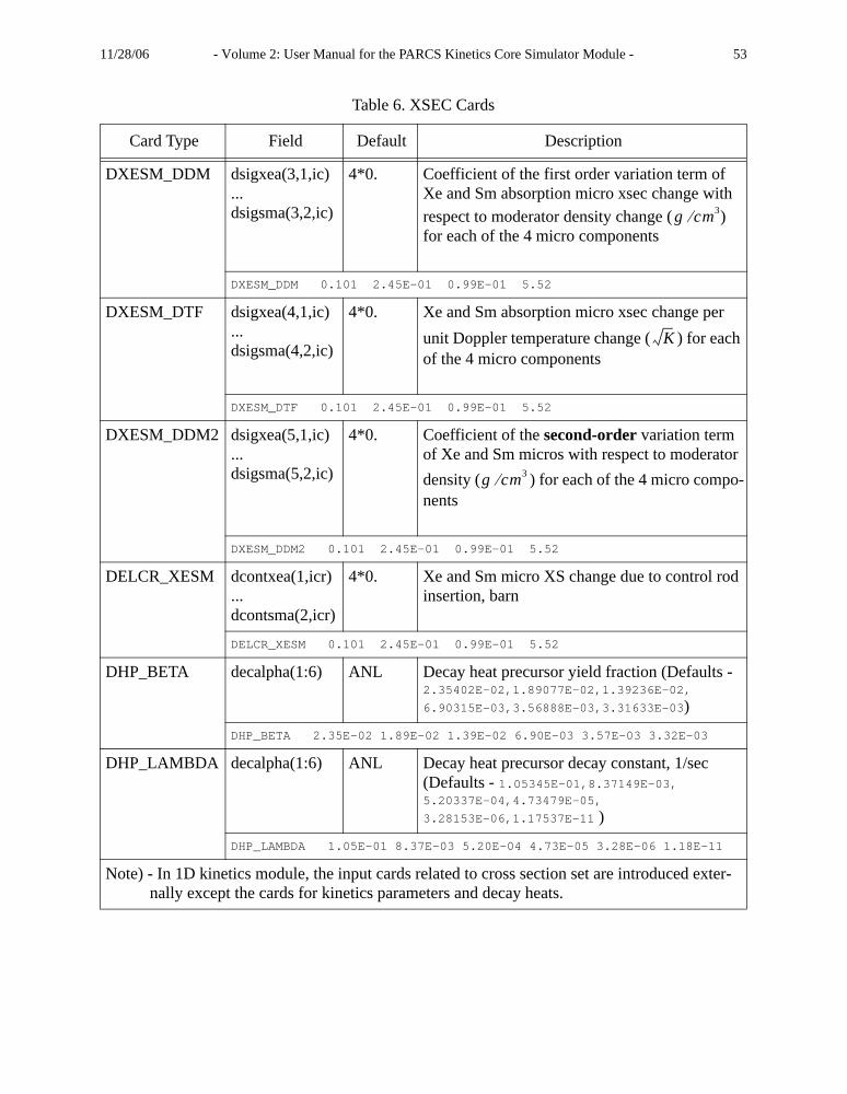
11/28/06 - Volume 2: User Manual for the PARCS Kinetics Core Simulator Module - 53
DXESM_DDM dsigxea(3,1,ic)...dsigsma(3,2,ic)
4*0. Coefficient of the first order variation term of Xe and Sm absorption micro xsec change with respect to moderator density change ( ) for each of the 4 micro components
DXESM_DDM 0.101 2.45E-01 0.99E-01 5.52
DXESM_DTF dsigxea(4,1,ic)...dsigsma(4,2,ic)
4*0. Xe and Sm absorption micro xsec change per unit Doppler temperature change ( ) for each of the 4 micro components
DXESM_DTF 0.101 2.45E-01 0.99E-01 5.52
DXESM_DDM2 dsigxea(5,1,ic)...dsigsma(5,2,ic)
4*0. Coefficient of the second-order variation term of Xe and Sm micros with respect to moderator density ( ) for each of the 4 micro compo-nents
DXESM_DDM2 0.101 2.45E-01 0.99E-01 5.52
DELCR_XESM dcontxea(1,icr)...dcontsma(2,icr)
4*0. Xe and Sm micro XS change due to control rod insertion, barn
DELCR_XESM 0.101 2.45E-01 0.99E-01 5.52
DHP_BETA decalpha(1:6) ANL Decay heat precursor yield fraction (Defaults - 2.35402E-02,1.89077E-02,1.39236E-02,
6.90315E-03,3.56888E-03,3.31633E-03)
DHP_BETA 2.35E-02 1.89E-02 1.39E-02 6.90E-03 3.57E-03 3.32E-03
DHP_LAMBDA decalpha(1:6) ANL Decay heat precursor decay constant, 1/sec (Defaults - 1.05345E-01,8.37149E-03,5.20337E-04,4.73479E-05,3.28153E-06,1.17537E-11 )
DHP_LAMBDA 1.05E-01 8.37E-03 5.20E-04 4.73E-05 3.28E-06 1.18E-11
Note) - In 1D kinetics module, the input cards related to cross section set are introduced exter-nally except the cards for kinetics parameters and decay heats.
Table 6. XSEC Cards
Card Type Field Default Description
g cm3⁄
K
g cm3⁄

11/28/06 - Volume 2: User Manual for the PARCS Kinetics Core Simulator Module - 54
DDDC dddc_comp_num none Number of compositions for which directional diffusion coefficients will be applied
dddccfr none Factor to be multiplied by the diffusion coeffi-cient in the radial direction
dddccfz none Factor to be multiplied by the diffusion coeffi-cient in the axial direction
DDDC 7 0.1 0.5
Table 6. XSEC Cards
Card Type Field Default Description

11/28/06 - Volume 2: User Manual for the PARCS Kinetics Core Simulator Module - 55
Table 7. GEOM Cards
Card Type Field Default Description
GEO_DIM nasyx 2 Number of assemblies in x-direction
nasyy 1 Number of assemblies in y-direction
nz 1 Number of planes in z-direction
nzbr 0 Number of planes for bottom reflector
nztr 0 Number of planes for top reflector
GEO_DIM 9 9 20 1 1
SYMMETRY isymmetry 1 Symmetry option for rectangular geometries: 1 == full core 2 == half core 4 == quarter core
RAD_CONF iradconf (1:nasyx, 1:nasyy)
None Radial core configuration 0 - dummy region 1 - reflector region >1 - fuel region
RAD_CONF 2 2 2 2 2 2 2 2 1 2 2 2 2 2 2 2 2 1 2 2 2 2 2 2 2 1 1 2 2 2 2 2 2 2 1 0 2 2 2 2 2 2 1 1 0 2 2 2 2 2 1 1 0 0 2 2 2 2 1 1 0 0 0 2 2 1 1 1 0 0 0 0 1 1 1 0 0 0 0 0 0
COORDINATE idum 1 Coordinate system of the problem: 1 == cartesian 2 == cylindrical
GRID_Xor GRID_R
hasyx(1:nasyx) nasyx*10 Mesh spacing in x-direction (cartesian) or r-direction (cylindrical), cm
GRID_X 10.803 8*21.606 GRID_R 78.6 32.3 24.8 20.9 18.4 6.0 13.0 21.0 20.0 15.0 25.0
GRID_Yor GRID_THETA
hasyy(1:nasyy) 1 Mesh spacing in y-direction (cartesian) in cm or theta-direction (cylindrical) in degrees
GRID_Y 10.803 8*21.606 GRID_THETA 1#3.0

11/28/06 - Volume 2: User Manual for the PARCS Kinetics Core Simulator Module - 56
GRID_Z hz(1:nz) 1 Axial node size, cm
GRID_Z 10.803 8*21.606
NEUTMESH_Xor NEUTMESH_R
nneutx(1:nasyx) nasyx*1 Number of neutronic mesh per assembly or coarse mesh in -x or -r direction
NEUTMESH_X 1 8*2 NEUTMESH_R 1 1 1 1 1 1 1 1 1 1 1
NEUTMESH_YorNEUTMESH_THETA
nneuty(1:nasyy) nasyy*1 Number of neutronic mesh per assembly or coarse mesh in -y or -theta direction.
NEUTMESH_Y 1 8*2NEUTMESH_THETA 1*1
BOUN_COND ibcx(1:2) 2*0 Boundary conditions for left (1) and right (2) sides in each direction 0 - reflective 1 - zero flux 2 - zero incoming current 3 - Albedo(=Jin/Jout) 2x2 matrix (1DK and
z-direction only)* when 3 is chosen, ALBEDO_* card is needed.
ibcy(1:2) 2*0
ibcz(1:2) 2*0
BOUN_COND 0 2 0 2 2 2
ALBEDO_ZL,ALBEDO_ZR
alzl(1:4),alzr(1:4)
None 2x2 albedo matrix elements ((1,2);(3,4))at the left(bottom) and right(top) boundaries in z-direction. Internally, the second element is always set to zero assuming no upscattering.
ALBEDO_ZL 0.18732 0.0 -1.3535E-01 1.3925E-01ALBEDO_ZR 0.18732 0.0 -1.3535E-01 1.3925E-01
Table 7. GEOM Cards
Card Type Field Default Description

11/28/06 - Volume 2: User Manual for the PARCS Kinetics Core Simulator Module - 57
PLANAR_REG ipr None Planar region number
iprcomp(1:nxya,ipr)
Planar region compositions assigned to each non-dummy region of the radial configuration (RAD_CONF), better to be given in a 2D array form (nxya is the number of nonzeros in the RAD_CONF card)If depl is T in CNTL cards, the regions with same structure but different burnup will be assigned to same composition number.
PLANAR_REG 2 4 5 4 5 4 5 4 6 2 5 4 5 4 5 4 6 6 2 4 5 4 5 4 5 6 3 2 5 4 5 4 5 6 6 2 4 5 4 5 4 6 3 2 5 4 5 6 6 3 2 4 6 6 6 3 2 6 6 3 2 2 2 2 2
PR_ASSIGN izpr(1:nz) None Planar region assignment to each plane
PR_ASSIGN 1 2 15*3 1 ! for 18 planes
CR_AXINFO(Control Rod Axial Info.)
crbpos0 0.0 Control rod full insertion position from the bottom (PWR) or top (BWR) of the core (including reflector), cm
crbstep 1.0 Control rod step size, cm
CR_AXINFO 25.0 0.15
BANK_CONF iradconf(:,1:nasyy)
nxya*0 Control rod banks defined for each non-dummy region of the radial configuration, 0 means no bank defined
BANK_CONF 1 0 2 0 0 0 3 0 0 0 4 0 0 0 6 0 0 0 2 0 5 0 6 0 6 0 0 0 0 0 4 0 0 0 0 0 0 6 0 7 0 0 0 0 6 0 0 0 0 0 3 0 6 0 0 0 0 0 0 0 0 0 0 0
Table 7. GEOM Cards
Card Type Field Default Description

11/28/06 - Volume 2: User Manual for the PARCS Kinetics Core Simulator Module - 58
PINCAL_LOC iradconf (:,1:nasyy)
nxya*0 Radial locations at which the pin power calcula-tion is to be performed, any nonzero value turns on pin power calculation at that location
PINCAL_LOC 1 0 2 0 0 0 3 0 0 0 4 0 0 0 6 0 0 0 2 0 5 0 6 0 6 0 0 0 0 0 4 0 0 0 0 0 0 6 0 7 0 0 0 0 6 0 0 0 0 0 3 0 6 0 0 0 0 0 0 0 0 0 0 0
CRB_DEF ncrbtypeitypeicrbcmp(itype,:)cmplnth(itype,:)
1111.0E+30
The number of CRB types defined in this card.CRB type index.The composition ID’s for the CRB type itype.The lengths of the compositions.
CRB_DEF 2 1 0 1 2.994 365.056 2 0 2 1 2.994 14.602 350.454
CRB_TYPE icrbtype(1:ncrb) 1 The CRB types for each control rod banks.
CRB_TYPE 1 2 1 1 1 1 2 1 2 1
ADF_ROT nrotfa (:,1:nasyy)
nxya*0 The index of assembly rotation : 0/1/2/3 means rotate assembly 0/90/180/270 degree anti-clock wise.
ADF_ROT 1 2 3 0
DET_XY_LOC nxydet 0 Total number of detectors.
ndetfa (1:nasyx,1:nasyy)
nxya*0 Radial location at which detector response is to be calculated ( any non-zero value turns on detector response calculation at that location, assemblies contributing to the same detector response are grouped by non-zero value )
DET_XY_LOC 12 1 1 2 2 1 1 2 2 0 0 3 3 0 0 3 3
Table 7. GEOM Cards
Card Type Field Default Description
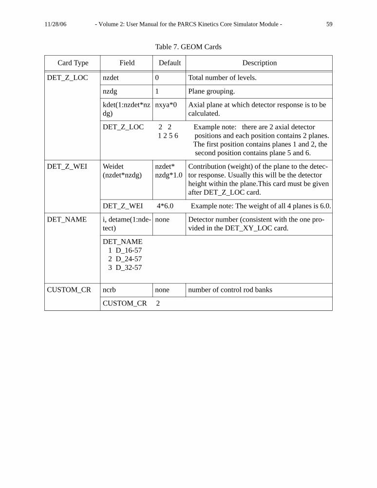
11/28/06 - Volume 2: User Manual for the PARCS Kinetics Core Simulator Module - 59
DET_Z_LOC nzdet 0 Total number of levels.
nzdg 1 Plane grouping.
kdet(1:nzdet*nzdg)
nxya*0 Axial plane at which detector response is to be calculated.
DET_Z_LOC 2 2 Example note: there are 2 axial detector 1 2 5 6 positions and each position contains 2 planes. The first position contains planes 1 and 2, the second position contains plane 5 and 6.
DET_Z_WEI Weidet(nzdet*nzdg)
nzdet*nzdg*1.0
Contribution (weight) of the plane to the detec-tor response. Usually this will be the detectorheight within the plane.This card must be given after DET_Z_LOC card.
DET_Z_WEI 4*6.0 Example note: The weight of all 4 planes is 6.0.
DET_NAME i, detame(1:nde-tect)
none Detector number (consistent with the one pro-vided in the DET_XY_LOC card.
DET_NAME 1 D_16-57 2 D_24-57 3 D_32-57
CUSTOM_CR ncrb none number of control rod banks
CUSTOM_CR 2
Table 7. GEOM Cards
Card Type Field Default Description

11/28/06 - Volume 2: User Manual for the PARCS Kinetics Core Simulator Module - 60
CCR_BANK ib none |ib| is the bank indexIf ib<0, this bank will remain out during scram
levels none Number of levels of the path of this bank. The levels are defined in the following cards.
gt 0 The control rod composition index for the guide tube.Note: 0 indicates that the guide tube is not treated
The following fields of this card are repeated for each level
dist none distance from the far end of this level to the tip of the fully inserted rod position
nodes none Number of nodes traversed by this rod bank at this level. "node" sets consisting of three num-bers (la, k, f) will be given in this line after the "nodes" entry.
l none assembly index in x-y or hex plane
k none axial plane index
f none total rod fraction when control rod passes through the node
CCR_BANK -1 3 0 30.0 3 1 3 1.0 2 3 1.0 3 3 1.060.0 3 1 2 1.0 2 2 1.0 3 2 1.090.0 3 1 1 1.0 2 1 1.0 3 1 1.0
Note) - For 1D kinetics module, the z-direction information from the GEO_DIM, GRID_Z, BOUN_COND, CR_AXINFO cards is transferred to the 1D module.
Table 8. PFF Cards
Card Type Field Default Description
NPIN_SIDE npin None Number of fuel pins along a side of an assembly
NPIN_SIDE 17.0
Table 7. GEOM Cards
Card Type Field Default Description
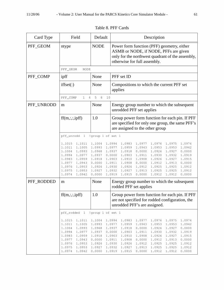
11/28/06 - Volume 2: User Manual for the PARCS Kinetics Core Simulator Module - 61
PFF_GEOM ntype NODE Power form function (PFF) geometry, either ASMB or NODE, if NODE, PFFs are given only for the northwest quadrant of the assembly, otherwise for full assembly.
PFF_GEOM NODE
PFF_COMP ipff None PFF set ID
iffset(:) None Compositions to which the current PFF set applies
PFF_COMP 1 4 5 6 10
PFF_UNRODD m None Energy group number to which the subsequent unrodded PFF set applies
ff(m,:,:,ipff) 1.0 Group power form function for each pin. If PFF are specified for only one group, the same PFF’s are assigned to the other group
pff_unrodd 1 !group 1 of set 1
1.1015 1.1011 1.1004 1.0994 1.0983 1.0977 1.0976 1.0975 1.09741.1011 1.1005 1.0993 1.0977 1.0959 1.0943 1.0953 1.0953 1.09421.1004 1.0993 1.0968 1.0937 1.0918 0.0000 1.0926 1.0927 0.00001.0994 1.0977 1.0937 0.0000 1.0903 1.0911 1.0930 1.0932 1.09191.0983 1.0959 1.0918 1.0903 1.0910 1.0908 1.0926 1.0927 1.09151.0977 1.0943 0.0000 1.0911 1.0908 0.0000 1.0912 1.0913 0.00001.0976 1.0953 1.0926 1.0930 1.0926 1.0912 1.0925 1.0925 1.09121.0975 1.0953 1.0927 1.0932 1.0927 1.0913 1.0925 1.0925 1.09121.0974 1.0942 0.0000 1.0919 1.0915 0.0000 1.0912 1.0912 0.0000
PFF_RODDED m None Energy group number to which the subsequent rodded PFF set applies
ff(m,:,:,ipff) 1.0 Group power form function for each pin. If PFF are not specified for rodded configuration, the unrodded PFF’s are assigned.
pff_rodded 1 !group 1 of set 1
1.1015 1.1011 1.1004 1.0994 1.0983 1.0977 1.0976 1.0975 1.09741.1011 1.1005 1.0993 1.0977 1.0959 1.0943 1.0953 1.0953 1.09421.1004 1.0993 1.0968 1.0937 1.0918 0.0000 1.0926 1.0927 0.00001.0994 1.0977 1.0937 0.0000 1.0903 1.0911 1.0930 1.0932 1.09191.0983 1.0959 1.0918 1.0903 1.0910 1.0908 1.0926 1.0927 1.09151.0977 1.0943 0.0000 1.0911 1.0908 0.0000 1.0912 1.0913 0.00001.0976 1.0953 1.0926 1.0930 1.0926 1.0912 1.0925 1.0925 1.09121.0975 1.0953 1.0927 1.0932 1.0927 1.0913 1.0925 1.0925 1.09121.0974 1.0942 0.0000 1.0919 1.0915 0.0000 1.0912 1.0912 0.0000
Table 8. PFF Cards
Card Type Field Default Description

11/28/06 - Volume 2: User Manual for the PARCS Kinetics Core Simulator Module - 62
Table 9. TRAN Cards
Card Type Field Default Description
TIME_STEP tend None Transient duration, sec
delt0 None Initial time step size, sec
tswitch None Time when to switch to new time step size, sec
texpand None Expansion factor for new time step size
TIME_STEP 100.0 0.01 20.0 10.0
EXPO_OPT exptrsf F Exponential transform option, T or F
expextp T Exponential extrapolation option, T or F
EXPO_OPT F T
THETA cetak 0.5 value for kinetics
cetac 1.0 value for coolant T/H
cetaf 0.5 value for fuel heat conduction
THETA 0.5 1.0 0.5
CONV_TR
(Transient Con-vergence Crite-ria)
epsr2 0.001 Residual convergence criterion
epsl2t epsl2 Global fission source convergence criterion
epslinft epslinf Local fission source convergence criterion
epstft epstf Fuel temperature convergence criterion
CONV_TR 0.001 0.002 1e-04 1e-6
NLUPD_TR nupdcyt 5 Nonlinear update cycle (e.g. every 5 iterations)
ninitoutt 1 Number of iterations to be performed before the first nonlinear update
numltht 5 Number of T/H updates per nodal update
nthmax 10 Maximum number of fuel heat conduction cal-culations per time step
NLUPD_TR 5 1 5 10
EPS_XSEC epsxsec 0.01 Cross section change criterion for requiring at least one nodal update
EPS_XSEC 0.01
θ
θ
θ
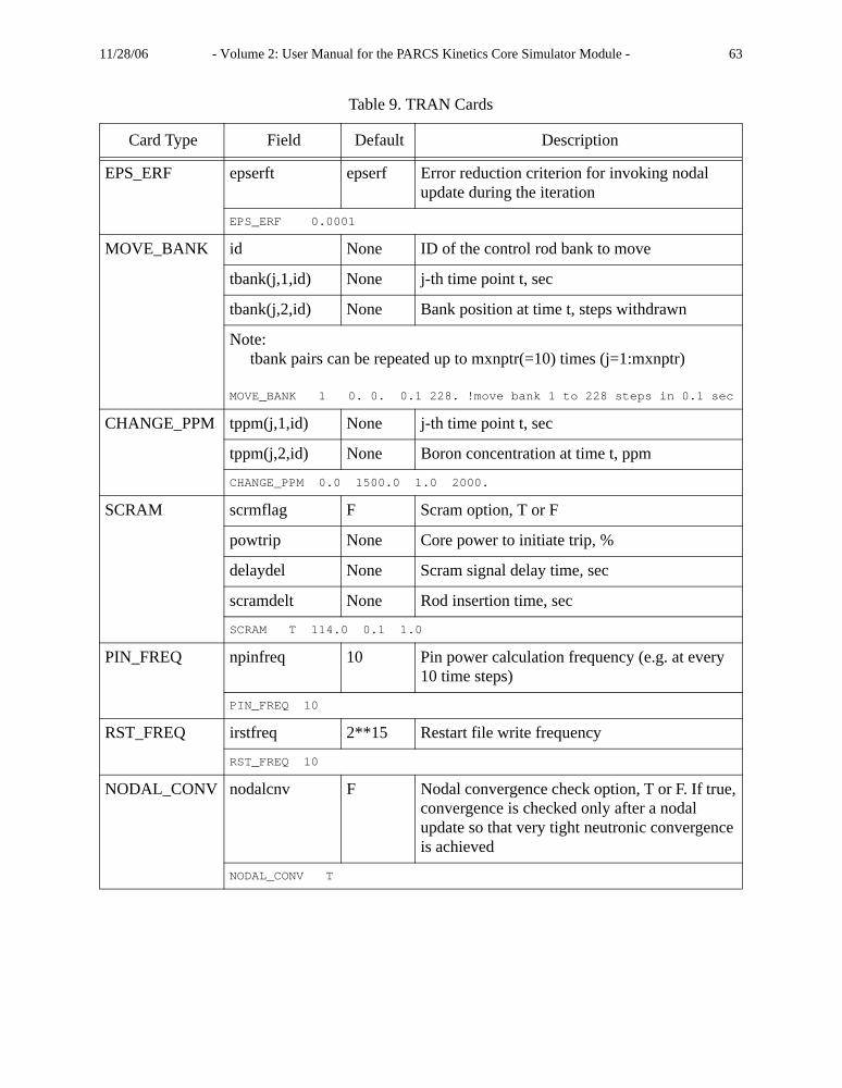
11/28/06 - Volume 2: User Manual for the PARCS Kinetics Core Simulator Module - 63
EPS_ERF epserft epserf Error reduction criterion for invoking nodal update during the iteration
EPS_ERF 0.0001
MOVE_BANK id None ID of the control rod bank to move
tbank(j,1,id) None j-th time point t, sec
tbank(j,2,id) None Bank position at time t, steps withdrawn
Note: tbank pairs can be repeated up to mxnptr(=10) times (j=1:mxnptr)
MOVE_BANK 1 0. 0. 0.1 228. !move bank 1 to 228 steps in 0.1 sec
CHANGE_PPM tppm(j,1,id) None j-th time point t, sec
tppm(j,2,id) None Boron concentration at time t, ppm
CHANGE_PPM 0.0 1500.0 1.0 2000.
SCRAM scrmflag F Scram option, T or F
powtrip None Core power to initiate trip, %
delaydel None Scram signal delay time, sec
scramdelt None Rod insertion time, sec
SCRAM T 114.0 0.1 1.0
PIN_FREQ npinfreq 10 Pin power calculation frequency (e.g. at every 10 time steps)
PIN_FREQ 10
RST_FREQ irstfreq 2**15 Restart file write frequency
RST_FREQ 10
NODAL_CONV nodalcnv F Nodal convergence check option, T or F. If true, convergence is checked only after a nodal update so that very tight neutronic convergence is achieved
NODAL_CONV T
Table 9. TRAN Cards
Card Type Field Default Description
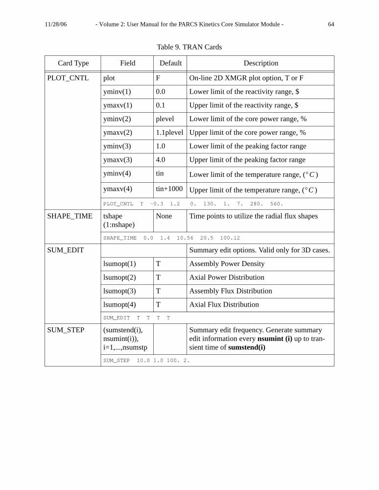
11/28/06 - Volume 2: User Manual for the PARCS Kinetics Core Simulator Module - 64
PLOT_CNTL plot F On-line 2D XMGR plot option, T or F
yminv(1) 0.0 Lower limit of the reactivity range, $
ymaxv(1) 0.1 Upper limit of the reactivity range, $
yminv(2) plevel Lower limit of the core power range, %
ymaxv(2) 1.1plevel Upper limit of the core power range, %
yminv(3) 1.0 Lower limit of the peaking factor range
ymaxv(3) 4.0 Upper limit of the peaking factor range
yminv(4) tin Lower limit of the temperature range, ( )
ymaxv(4) tin+1000 Upper limit of the temperature range, ( )
PLOT_CNTL T -0.3 1.2 0. 130. 1. 7. 280. 560.
SHAPE_TIME tshape(1:nshape)
None Time points to utilize the radial flux shapes
SHAPE_TIME 0.0 1.4 10.56 20.5 100.l2
SUM_EDIT Summary edit options. Valid only for 3D cases.
lsumopt(1) T Assembly Power Density
lsumopt(2) T Axial Power Distribution
lsumopt(3) T Assembly Flux Distribution
lsumopt(4) T Axial Flux Distribution
SUM_EDIT T T T T
SUM_STEP (sumstend(i), nsumint(i)), i=1,...,nsumstp
Summary edit frequency. Generate summary edit information every nsumint (i) up to tran-sient time of sumstend(i)
SUM_STEP 10.0 1.0 100. 2.
Table 9. TRAN Cards
Card Type Field Default Description
°C
°C
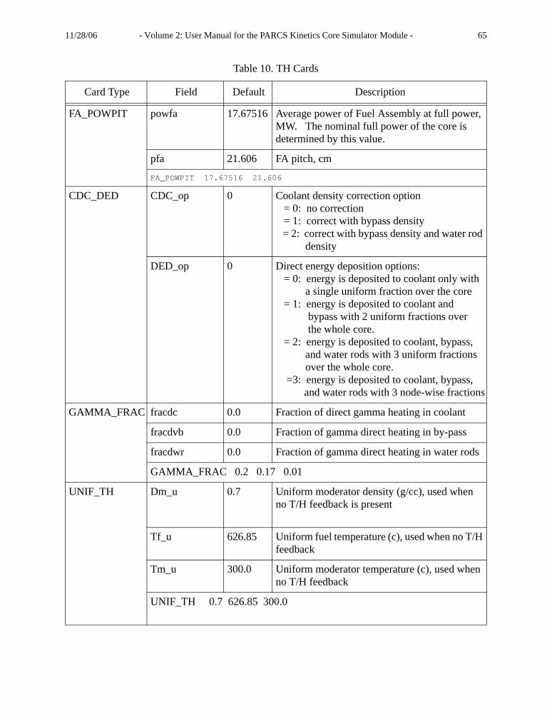
11/28/06 - Volume 2: User Manual for the PARCS Kinetics Core Simulator Module - 65
Table 10. TH Cards
Card Type Field Default Description
FA_POWPIT powfa 17.67516 Average power of Fuel Assembly at full power, MW. The nominal full power of the core is determined by this value.
pfa 21.606 FA pitch, cm
FA_POWPIT 17.67516 21.606
CDC_DED CDC_op 0 Coolant density correction option = 0: no correction = 1: correct with bypass density = 2: correct with bypass density and water rod density
DED_op 0 Direct energy deposition options: = 0: energy is deposited to coolant only with a single uniform fraction over the core = 1: energy is deposited to coolant and bypass with 2 uniform fractions over the whole core. = 2: energy is deposited to coolant, bypass, and water rods with 3 uniform fractions over the whole core. =3: energy is deposited to coolant, bypass, and water rods with 3 node-wise fractions
GAMMA_FRAC fracdc 0.0 Fraction of direct gamma heating in coolant
fracdvb 0.0 Fraction of gamma direct heating in by-pass
fracdwr 0.0 Fraction of gamma direct heating in water rods
GAMMA_FRAC 0.2 0.17 0.01
UNIF_TH Dm_u 0.7 Uniform moderator density (g/cc), used when no T/H feedback is present
Tf_u 626.85 Uniform fuel temperature (c), used when no T/H feedback
Tm_u 300.0 Uniform moderator temperature (c), used when no T/H feedback
UNIF_TH 0.7 626.85 300.0

11/28/06 - Volume 2: User Manual for the PARCS Kinetics Core Simulator Module - 66
FLU_TYP fluid_typ 0 Coolant option:0: Light Water (P=15.5 MPa, 280 < T [C] < 3401: Heavy Water (P=11.6 MPa, 260 < T[C] < 320
fluid_typ 1
Table 11. DEPL Cards
Card Type Field Default Description
INP_HST InpHst_na None Name of Input file which contains history and TH state information
Table 10. TH Cards
Card Type Field Default Description

11/28/06 - Volume 2: User Manual for the PARCS Kinetics Core Simulator Module - 67
InpHst_fm 0 0/1/2: binary/Ascii/SIMULATE-3The values of the history or TH state are givenafter the keywords:EXP 3D MAPHCR 3D MAPHDC3D MAPHPC 3D MAPHTF 3D MAPHTC 3D MAPDCO 3D MAPPCO 3D MAPTCO 3D MAPTFU 3D MAPXEN 3D MAPSMN 3D MAP
These 12 keywords are accepted by all later ver-sionsof PARCS. Some of the old keywords areno longer acceptable and should be changed bythe user as follows:HVO 3D MAP -> HDC 3D MAPHMD 3D MAP -> HDC 3D MAPHSB 3D MAP -> HPC 3D MAPDEN 3D MAP -> DCO 3D MAPSB 3D MAP -> PCO 3D MAPTM 3D MAP -> TCO 3D MAP* Read the note below
ResP 1 Restart from this point in file InpHst_na. The initial point is point 1.
INP_HST ‘DEP1.dep’ 1 3 1 2 3
Table 11. DEPL Cards
Card Type Field Default Description
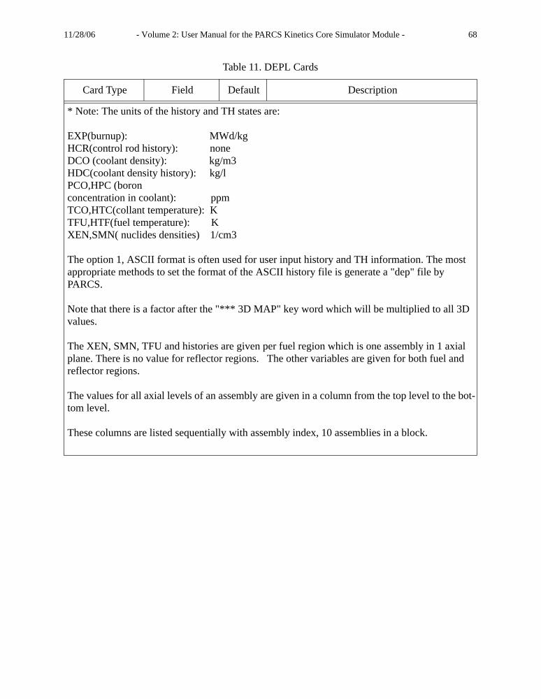
11/28/06 - Volume 2: User Manual for the PARCS Kinetics Core Simulator Module - 68
* Note: The units of the history and TH states are:
EXP(burnup): MWd/kgHCR(control rod history): noneDCO (coolant density): kg/m3HDC(coolant density history): kg/lPCO,HPC (boron concentration in coolant): ppmTCO,HTC(collant temperature): KTFU,HTF(fuel temperature): KXEN,SMN( nuclides densities) 1/cm3
The option 1, ASCII format is often used for user input history and TH information. The most appropriate methods to set the format of the ASCII history file is generate a "dep" file by PARCS.
Note that there is a factor after the "*** 3D MAP" key word which will be multiplied to all 3D values.
The XEN, SMN, TFU and histories are given per fuel region which is one assembly in 1 axial plane. There is no value for reflector regions. The other variables are given for both fuel and reflector regions.
The values for all axial levels of an assembly are given in a column from the top level to the bot-tom level.
These columns are listed sequentially with assembly index, 10 assemblies in a block.
Table 11. DEPL Cards
Card Type Field Default Description
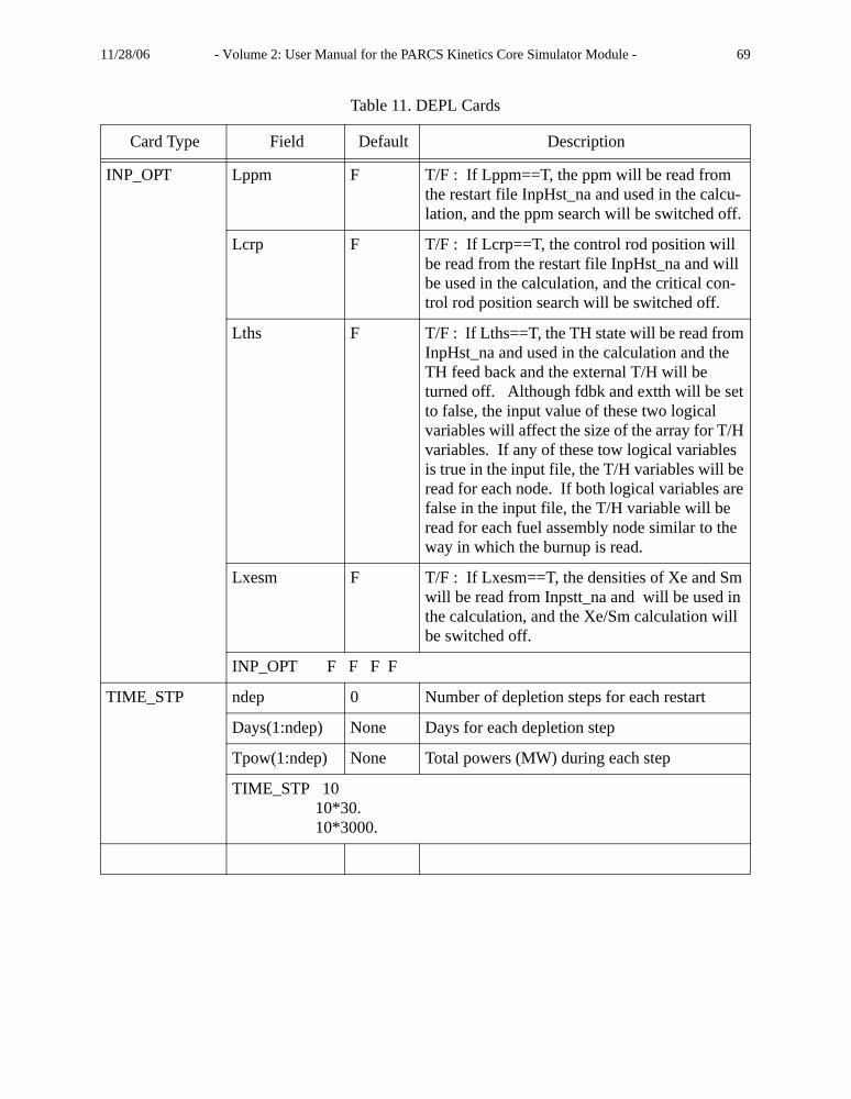
11/28/06 - Volume 2: User Manual for the PARCS Kinetics Core Simulator Module - 69
INP_OPT Lppm F T/F : If Lppm==T, the ppm will be read from the restart file InpHst_na and used in the calcu-lation, and the ppm search will be switched off.
Lcrp F T/F : If Lcrp==T, the control rod position will be read from the restart file InpHst_na and will be used in the calculation, and the critical con-trol rod position search will be switched off.
Lths F T/F : If Lths==T, the TH state will be read from InpHst_na and used in the calculation and the TH feed back and the external T/H will be turned off. Although fdbk and extth will be set to false, the input value of these two logical variables will affect the size of the array for T/H variables. If any of these tow logical variables is true in the input file, the T/H variables will be read for each node. If both logical variables are false in the input file, the T/H variable will be read for each fuel assembly node similar to the way in which the burnup is read.
Lxesm F T/F : If Lxesm==T, the densities of Xe and Sm will be read from Inpstt_na and will be used in the calculation, and the Xe/Sm calculation will be switched off.
INP_OPT F F F F
TIME_STP ndep 0 Number of depletion steps for each restart
Days(1:ndep) None Days for each depletion step
Tpow(1:ndep) None Total powers (MW) during each step
TIME_STP 10 10*30. 10*3000.
Table 11. DEPL Cards
Card Type Field Default Description
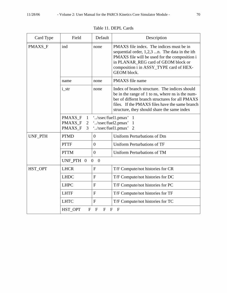
11/28/06 - Volume 2: User Manual for the PARCS Kinetics Core Simulator Module - 70
PMAXS_F ind none PMAXS file index. The indices must be in sequential order, 1,2,3 ...n. The data in the ith PMAXS file will be used for the composition i in PLANAR_REG card of GEOM block or composition i in ASSY_TYPE card of HEX-GEOM block.
name none PMAXS file name
i_str none Index of branch structure. The indices should be in the range of 1 to ns, where ns is the num-ber of differnt branch structures for all PMAXS files. If the PMAXS files have the same branch structure, they should share the same index
PMAXS_F 1 ‘../xsec/fuel1.pmax’ 1PMAXS_F 2 ‘../xsec/fuel2.pmax’ 1PMAXS_F 3 ‘../xsec/fuel1.pmax’ 2
UNF_PTH PTMD 0 Uniform Perturbations of Dm
PTTF 0 Uniform Perturbations of TF
PTTM 0 Uniform Perturbations of TM
UNF_PTH 0 0 0
HST_OPT LHCR F T/F Compute/not histories for CR
LHDC F T/F Compute/not histories for DC
LHPC F T/F Compute/not histories for PC
LHTF F T/F Compute/not histories for TF
LHTC F T/F Compute/not histories for TC
HST_OPT F F F F F
Table 11. DEPL Cards
Card Type Field Default Description
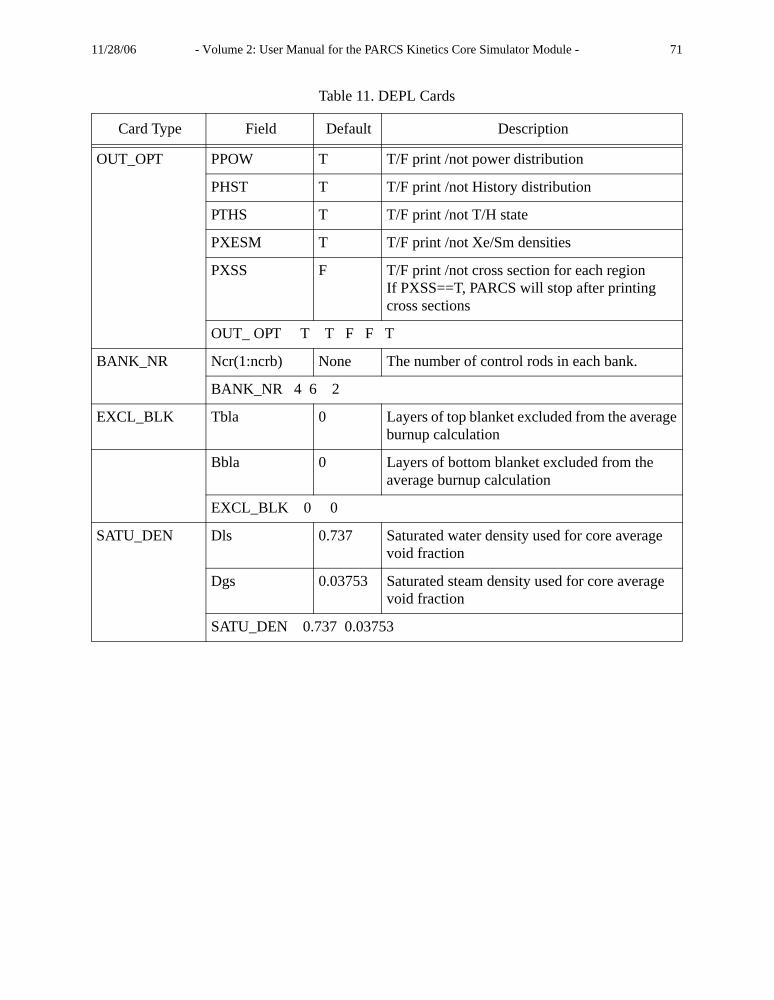
11/28/06 - Volume 2: User Manual for the PARCS Kinetics Core Simulator Module - 71
OUT_OPT PPOW T T/F print /not power distribution
PHST T T/F print /not History distribution
PTHS T T/F print /not T/H state
PXESM T T/F print /not Xe/Sm densities
PXSS F T/F print /not cross section for each regionIf PXSS==T, PARCS will stop after printing cross sections
OUT_ OPT T T F F T
BANK_NR Ncr(1:ncrb) None The number of control rods in each bank.
BANK_NR 4 6 2
EXCL_BLK Tbla 0 Layers of top blanket excluded from the average burnup calculation
Bbla 0 Layers of bottom blanket excluded from the average burnup calculation
EXCL_BLK 0 0
SATU_DEN Dls 0.737 Saturated water density used for core average void fraction
Dgs 0.03753 Saturated steam density used for core average void fraction
SATU_DEN 0.737 0.03753
Table 11. DEPL Cards
Card Type Field Default Description

11/28/06 - Volume 2: User Manual for the PARCS Kinetics Core Simulator Module - 72
Table 12. PLOT Cards (Only for QuickWin Based Graphics)
Card Type Field Default Description
XTYPE ixtype 0 Type of the x-axis in the X-Y plot 0 - Time 1 - Reserved 2 - Case Index
x_min 0 Minimum value on the x-axis
x_max tend Maximum value on the x-axis. Equal to the full simulation time if ixtype equals to 0.
XTYPE 0 0 100.0
XTYPE 2 0 5.0

11/28/06 - Volume 2: User Manual for the PARCS Kinetics Core Simulator Module - 73
XY alpid None Alphanumeric ID of the variable for which an X-Y plot is made, one of the following: keff - k-effective plevel - normalized core power level rhoadj - reactivity toutavg - average coolant exit temperature dmrho - density component reactivity tmrho - coolant temperature comp. reactivity tfrho - fuel temperature comp. reactivity crrho - control rod comp. reactivity ppmrho - ppm comp. reactivity crbpos(i) - i-th control bank position tcool - coolant temperature vector dcool - coolant density vector tfuel - fuel temperaure vector relp - relative power density vector flux1 - fast flux vector flux2 - thermal flux vector lp2d - fuel loading pattern crpmap - conrol bank position map
kklll None Vector index designating the location in the core at which the variable is obtained. kk designates the plane index and lll designate the radial node index. For scalar variables, enter 0.
y_min None Minimum y-axis value.
y_max None Maximum y-axis value.
iframe None X-Y plot frame number to which the curve belongs.
igraph None The color for designated curve number.
Table 12. PLOT Cards (Only for QuickWin Based Graphics)
Card Type Field Default Description
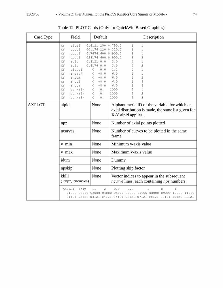
11/28/06 - Volume 2: User Manual for the PARCS Kinetics Core Simulator Module - 74
XY tfuel 014121 250.0 750.0 1 1XY tcool 001176 220.0 320.0 1 1XY dcool 017676 600.0 900.0 3 1XY dcool 028176 600.0 900.0 3 3XY relp 014121 0.0 3.0 4 1 XY relp 014176 0.0 3.0 4 2 XY plevel 0 0.0 1.2 5 1 XY rhoadj 0 -8.0 6.0 6 1XY rhodm 0 -8.0 6.0 6 2XY rhotf 0 -8.0 6.0 6 3XY rhocr 0 -8.0 6.0 6 4XY bank(1) 0 0. 1000 9 1XY bank(2) 0 0. 1000 9 2XY bank(3) 0 0. 1000 9 3
AXPLOT alpid None Alphanumeric ID of the variable for which an axial distribution is made, the same list given for X-Y alpid applies.
npz None Number of axial points plotted
ncurves None Number of curves to be plotted in the same frame
y_min None Minimum y-axis value
y_max None Maximum y-axis value
idum None Dummy
npskip None Plotting skip factor
kklll(1:npz,1:ncurves)
None Vector indices to appear in the subsequent ncurve lines, each containing npz numbers
AXPLOT relp 11 2 0.0 2.0 1 0 1 01000 02000 03000 04000 05000 06000 07000 08000 09000 10000 11000 01121 02121 03121 04121 05121 06121 07121 08121 09121 10121 11121
Table 12. PLOT Cards (Only for QuickWin Based Graphics)
Card Type Field Default Description

11/28/06 - Volume 2: User Manual for the PARCS Kinetics Core Simulator Module - 75
* Note that a full core plot can be obtained from a quarter core calculation by placing the quartercore based vector indices in the full core configuration. The radial node numbers for lp2d and crp-map do not count radial reflector nodes. The feedback variables (tcool, dcool, and tfuel), and rela-tive power density (relp) are defined only for T-H nodes. The radial reflectors are not counted inthe numbering, but in the coupled case, reflector nodes are assigned a node number.
RECTMAPCONTOURBITMAP
alpid None Alphanumeric ID of the variable for which a radial map based on rectangles (RECTMAP), or contour (CONTOUR), or color-filled contour (BITMAP) is made, the same list given in X-Y alpid holds.
npx None Number of Data Sets in the x-direction
npy None Number of Data Sets in the y-direction
z_min None Minimum z value where z=f(x,y)
z_max None Maximum z value
ncolor None Color skip factor
npskip 1 Radial Map Skip Factor, radial maps are updated once per every npskip time steps
kklll(1:npx,1:npy)
None Vector indices to appear in the subsequent npy lines, each containing npx numbers
RECTMAP tcool 8 7 220.0 300.0 0 1 00000 00000 00000 00000 00000 01001 01002 01003 00000 00000 00000 01008 01009 01010 01011 01012 00000 00000 01019 01020 01021 01022 01023 01024 00000 01032 01033 01034 01035 01036 01037 01038 00000 01047 01048 01049 01050 01051 01052 01053 01062 01063 01064 01065 01066 01067 01068 01069 01079 01080 01081 01082 01083 01084 01085 01086
Table 13. ONEDK Cards
Card Type Field Default Description
EXT_1DXS ext1dxs T Option to use external 1D cross section set
EXT_1DXS T
Table 12. PLOT Cards (Only for QuickWin Based Graphics)
Card Type Field Default Description

11/28/06 - Volume 2: User Manual for the PARCS Kinetics Core Simulator Module - 76
XS_FORM ixsform 0 Index for cross section form 0 : table form 1 : polynomial form (TRACM format) 2 : linear form
filename(14) None Input file name for cross section set
XS_FORM 1 tracin.xs
USE_CCF useccf F Option to use CCF
useccfcr F Option to use CCF for control rod
useccftf,useccfdm,useccfbo,useccftm,useccfpw,useccfbu,useccfxe
all F These options typically have a very minor impact on the result. Therefore it is valid to choose useccfcr as T to see the CCF effect.
use_ccf T T use_ccf F
CORE_DATA psys 155.0 System pressure in bar
bucur 0.0 Current core average exposure(MWD/MTU)
CORE_DATA 155.0 15.0
CORE_TH tinsub 0.0 Subcooling of inlet moderator temperature( )
CORE_TH 2.0
TRAC_INP tracinp F Option to use TRAC input
filename(17) None TRAC input filename
TRAC_INP T ../trac/tracin
EXT_1DSRC ext1dsrc F Option to use external 1D source for fixed source problem with external source(1D only)(valid for iptype=1 and tran=F)
filename(18) None External 1D source filename
content of 1D external source file :repeat for k=1, nz k, 1-group source, 2-group source
EXT_1DSRC T ./xsec/xsec.inp
Table 13. ONEDK Cards
Card Type Field Default Description
°C

11/28/06 - Volume 2: User Manual for the PARCS Kinetics Core Simulator Module - 77
DECUSP_FC irdfc
any CR possiblefor 1,...,ncrb
None Control rod ID to set the decusping function coefficients.A quadratic equation of control rod fraction in a node f(x)=a0+a1*x+a2*x*x, 0<f(x)<1, 0<x<1
dfc(irdfc,0) 0.4917 Zeroth order coefficient
dfc(irdfc,1) 0.1718 First order coefficient
dfc(irdfc,2) 0.3364 Second order coefficient
DECUSP_FC 1 0.4917 1.718E-01 0.3364
RAD_WEIGHT ifchan1d F Option to use channels in 1D kinetics module
nchan 1 Total number of channels defined in 1D module
ichweight 1 Index of channel weighting method (1:vol,2:sq-pow,3:user defined)
itfweight 1 Index of fuel temperature weighting method (1:vol,2:sq-pow,3:user defined)
filename(16) None Filename for power shape
RAD_WEIGHT T 3 1 2 ../trac/pow.shp
CHAN_AREA chvfrac(1:nchan)
1 for all channels
Each channel area fraction or channel area in any unit. They are normalized internally.
for quarter core of neacrp A1 problem including reflector region chan_area ! in m^2 0.0116705 0.0233410 0.0233410 0.0233410 0.0233410 0.0233410 0.0233410 0.0233410 0.0233410 0.0233410 0.0233410 0.0233410 0.0233410 0.0233410 0.0233410 0.0466819 0.0466819 0.0466819 0.0466819 0.0466819 0.0466819 0.0466819 0.0466819 0.0466819 0.0466819 0.0466819 0.0466819 0.0466819 0.0466819 0.0466819 0.0466819 0.0466819 0.0466819 0.0466819 0.0466819 0.0466819 0.0466819 0.0466819 0.0466819 0.0466819 0.0466819 0.0466819 0.0466819 0.0466819 0.0466819 0.0466819 0.0466819 0.7469108e-10
Table 13. ONEDK Cards
Card Type Field Default Description
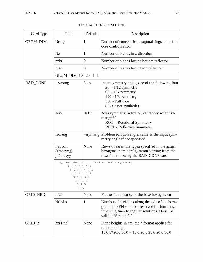
11/28/06 - Volume 2: User Manual for the PARCS Kinetics Core Simulator Module - 78
Table 14. HEXGEOM Cards
Card Type Field Default Description
GEOM_DIM Nring 1 Number of concentric hexagonal rings in the full core configuration
Nz 1 Number of planes in z-direction
nzbr 0 Number of planes for the bottom reflector
nztr 0 Number of planes for the top reflector
GEOM_DIM 10 26 1 1
RAD_CONF Isymang None Input symmetry angle, one of the following four 30 - 1/12 symmetry 60 - 1/6 symmetry 120 - 1/3 symmetry 360 - Full core (180 is not available)
Astr ROT Axis symmetry indicator, valid only when isy-mang=60 ROT - Rotational Symmetry REFL - Reflective Symmetry
Isolang =isymang Problem solution angle, same as the input sym-metry angle if not specified
iradconf (1:nasyx,j), j=1,nasyy
None Rows of assembly types specified in the actual hexagonal core configuration starting from the next line following the RAD_CONF card
rad_conf 60 rot !1/6 rotation symmetry 2 1 1 3 1 1 5 1 6 1 1 4 3 5 1 1 1 1 1 5 3 1 2 3 5 1 3 1 5 1 4 5 5 5
GRID_HEX hf2f None Flat-to-flat distance of the base hexagon, cm
Ndivhs 1 Number of divisions along the side of the hexa-gon for TPEN solution, reserved for future use involving finer triangular solutions. Only 1 is valid in Version 2.0
GRID_Z hz(1:nz) None Plane heights in cm, the * format applies for repetition. e.g.15.0 3*20.0 10.0 = 15.0 20.0 20.0 20.0 10.0
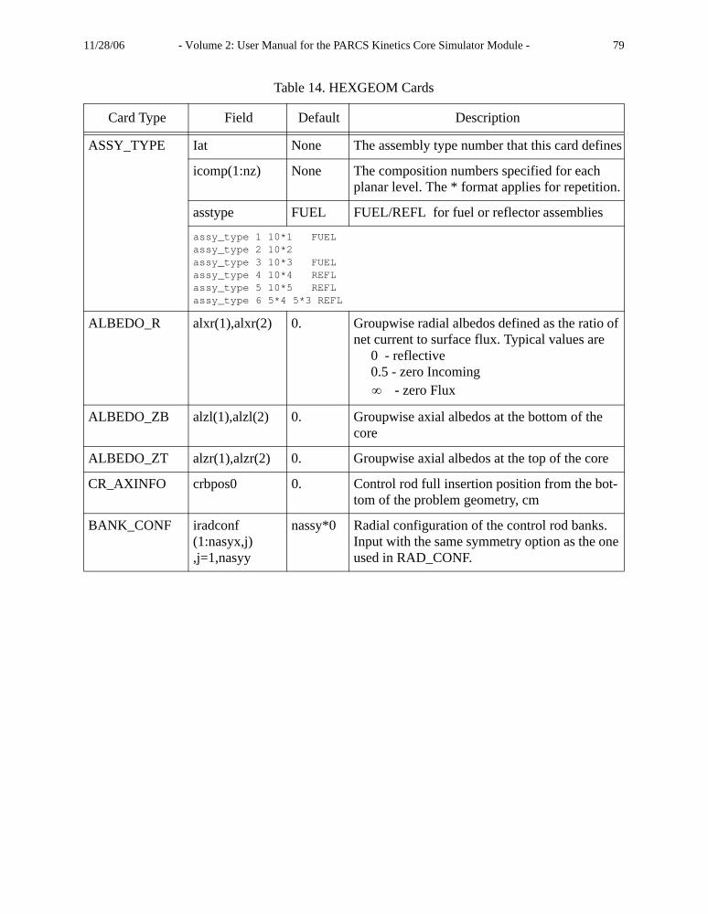
11/28/06 - Volume 2: User Manual for the PARCS Kinetics Core Simulator Module - 79
ASSY_TYPE Iat None The assembly type number that this card defines
icomp(1:nz) None The composition numbers specified for each planar level. The * format applies for repetition.
asstype FUEL FUEL/REFL for fuel or reflector assemblies
assy_type 1 10*1 FUELassy_type 2 10*2assy_type 3 10*3 FUELassy_type 4 10*4 REFLassy_type 5 10*5 REFLassy_type 6 5*4 5*3 REFL
ALBEDO_R alxr(1),alxr(2) 0. Groupwise radial albedos defined as the ratio of net current to surface flux. Typical values are 0 - reflective 0.5 - zero Incoming - zero Flux
ALBEDO_ZB alzl(1),alzl(2) 0. Groupwise axial albedos at the bottom of the core
ALBEDO_ZT alzr(1),alzr(2) 0. Groupwise axial albedos at the top of the core
CR_AXINFO crbpos0 0. Control rod full insertion position from the bot-tom of the problem geometry, cm
BANK_CONF iradconf (1:nasyx,j) ,j=1,nasyy
nassy*0 Radial configuration of the control rod banks. Input with the same symmetry option as the one used in RAD_CONF.
Table 14. HEXGEOM Cards
Card Type Field Default Description
∞

11/28/06 - Volume 2: User Manual for the PARCS Kinetics Core Simulator Module - 80
Table 15 FMFD CardsCard Type Field Default Description
GROUP_SPEC mg 2 Number of Groups. If this card ispresent, the multigroup option isturned on and the cross sections areread in the multigroup form thatinvolves scattering matrices
mge(1) mg/2 The last fine group number belongingto the first group in the two-groupstructure. If not speci-fied, mg/2 isused.
GENINF npins none Number of pin per FA sidenrefine 1 Number of mesh per pin sidemmz 1 Number of mesh per axial nodemeshth 1 TH meshes
1: thermal feedback in FA unitnpin: pin-by-pin thermal feedbak
METHOD npn 1 Order of angle 1: diffusion 3: SP3
naccel 2 Acceleration method 1: 2G coarse mesh rebalancing (CMR) 2: 2G coarse mesh finite difference (CMFD)
REF_COND ppmref 0. Reference boron concentration, ppmtmref 0. Reference moderator temperature,°Cdmref 0. Reference moderator density, g/cm3
tfref 0. Reference fuel temperature, °CDNP_NGRP nprec 6 Number of delayed neutron precursor
groupsBUCKLING buckling 0. Core bucklingNODALZ is2d1d F Activates 2d/1d coupling

11/28/06 - Volume 2: User Manual for the PARCS Kinetics Core Simulator Module - 81
Table 15 FMFD Cards (Cont.)Card Type Field Default Description
PLANAR_PIN ifacomp none FA composition numbericompf(1:npin*npin,ipr)
Planar region compositions assigned to each non-dummy region of the radial configuration (RAD_CONF) in a 2D array form (npin*npin is the number of non-zeros in the RAD_CONF card)
planar_pin 1 !UOX1 1 1 1 1 1 1 1 1 1 1 1 1 1 1 1 1 1 1 1 1 1 1 1 1 1 1 1 1 1 1 1 1 1 1 1 1 1 1 1 2 1 1 2 1 1 2 1 1 1 1 1 1 1 1 2 1 1 1 1 1 1 1 1 1 2 1 1 1 1 1 1 1 1 1 1 1 1 1 1 1 1 1 1 1 1 1 1 2 1 1 2 1 1 2 1 1 2 1 1 2 1 1 1 1 1 1 1 1 1 1 1 1 1 1 1 1 1 1 1 1 1 1 1 1 1 1 1 1 1 1 1 1 1 1 1 1 1 1 2 1 1 2 1 1 3 1 1 2 1 1 2 1 1 1 1 1 1 1 1 1 1 1 1 1 1 1 1 1 1 1 1 1 1 1 1 1 1 1 1 1 1 1 1 1 1 1 1 1 1 2 1 1 2 1 1 2 1 1 2 1 1 2 1 1 1 1 1 1 1 1 1 1 1 1 1 1 1 1 1 1 1 1 1 1 2 1 1 1 1 1 1 1 1 1 2 1 1 1 1 1 1 1 1 2 1 1 2 1 1 2 1 1 1 1 1 1 1 1 1 1 1 1 1 1 1 1 1 1 1 1 1 1 1 1 1 1 1 1 1 1 1 1 1 1 1 1 1 1 1
PIN_XSEC nmfpin none File name for pin cross sectionsipincomp Pin composition number
pin_xsec fmfd.UOX1.LF8-150b-8g 1

11/28/06 - Volume 2: User Manual for the PARCS Kinetics Core Simulator Module - 82
A schematic depicting the input card planar_pin necessary to provide pin by pin fuel compositions is shown below for a 13 assembly mini-core problem.
REF
REF
REF
REF
REF
REF
REF
REF
REF
REF
REFREF
UOX-1
UOX-1
UOX-1
UOX-1UOX-1
MOX-1
MOX-1
UOX-2(CR)
UOX-2(CR)
UOX-2(CR)
UOX-2(CR)
UOX-2(BA16)
MOX-1(BA8)
planar_reg 16 6 6 6 65 5 6 6 68 2 5 6 62 7 2 5 61 2 8 5 6
planar_pin 7 !MOX-1BA(Zoning)10 10 10 10 10 10 10 10 10 10 10 10 10 10 10 10 10 1 1 1 1 1 1 1 1 1 1 1 1 1 10 1 1 1 1 7 1 1 7 1 1 7 1 1 1 10 1 1 7 1 1 1 1 1 1 1 1 1 7 1 10 1 1 1 5 11 11 11 11 11 11 11 5 1 1 10 1 7 1 11 7 11 11 7 11 11 7 11 1 7 10 1 1 1 11 11 5 11 11 11 5 11 11 1 1 10 1 1 1 11 11 11 11 11 11 11 11 11 1 1 10 1 7 1 11 7 11 11 7 11 11 7 11 1 7 10 1 1 1 11 11 11 11 11 11 11 11 11 1 1 10 1 1 1 11 11 5 11 11 11 5 11 11 1 1 10 1 7 1 11 7 11 11 7 11 11 7 11 1 7 10 1 1 1 5 11 11 11 11 11 11 11 5 1 1 10 1 1 7 1 1 1 1 1 1 1 1 1 7 1 10 1 1 1 1 7 1 1 7 1 1 7 1 1 1 10 10 1 1 1 1 1 1 1 1 1 1 1 1 1 10 10 10 10 10 10 10 10 10 10 10 10 10 10 10
MOX 8.7%MOX 7.0%MOX 4.3 %Guide TubeBurnable Absorber

11/28/06 - Volume 2: User Manual for the PARCS Kinetics Core Simulator Module - 83
Table 16. Cross Sections Within PIN_XSEC File
Card Type Field Default Description{pin multigroup cross sections}
sigtr(ig,ic) 0. Transport cross sectionsiga(ig,ic) 0. Absorption cross sectionsignf(ig,ic) 0. Nu-fission cross sectionsigkf(ig,ic) 0. Kappa-fission cross sectionsigscat(ig,ig,ic) 0. Scattering cross sectionrambda(1:nprec,ic) 0. Delayed neutron precursor decay
constant, 1/secbeta(1:nprec,ic) 0. Delayed neutron fractionvelo(1:mg,ic) 0. Neutron velocity, cm/secsigchid(1:mg,1:nprec, ic)
0. Delayed neutron emission spectrum
sigchi(1:mg,ic) 0. Fission spectrumdsigtr(iv,ig,ic)….dsigkf(iv,ig,ic),dsigscat(iv,ig,ig,ic)
0. Macro XS change per unit moderator temperature change for each of cross section components
dsigtr(iv,ig,ic)….dsigkf(iv,ig,ic),dsigscat(iv,ig,ig,ic)
0. Macro XS change per unit Doppler temperature change for each of cross section components
dsigtr(iv,ig,ic)….dsigkf(iv,ig,ic),dsigscat(iv,ig,ig,ic)
0. Coefficient of the second-order variation term of Macro XS with respect to moderator density for each of cross section components
dsigtr(iv,ig,ic)….dsigkf(iv,ig,ic),dsigscat(iv,ig,ig,ic)
0. Macro XS change per unit ppm change for each of cross section components.
delcontr(iv,ig,ic)….delconkf(iv,ig,ic),delconscat(iv,ig,ig,ic)
0. Macro XS change due to control rod insertion

11/28/06 - Volume 2: User Manual for the PARCS Kinetics Core Simulator Module - 84
V.B MAPTAB Input Description
The coupling of the TRACE thermal-hydraulic mesh to the PARCS neutronic mesh is accom-plished through the assignment of mapping weights between the two mesh. These mappingweights, with values between 0 and 1, inclusive, determine the distribution of neutronic power inthe thermal-hydraulic and heat structure components, as well as the calculation of thermal-hydraulic feedback in the neutronic nodes. The determination of an accurate set of these weightsfor a particular problem is one of the most important tasks in achieving accurate coupled codesolutions with TRACE/PARCS.
V.B.1 Introduction
Two methods are currently available for determining the weights for a given thermal-hydraulic, heat structure, and neutronic nodalization: 1) an explicit weight method in which theuser is responsible for generating all weighting factors, and 2) an automated weight method inwhich the user provides only a minimal amount of mapping information and the code internalllygenerates the weighting factors. The automated method also generates the ASCII file MAPTABwith mapping information and weights which can then be modified by the user. The explicit andautomated weighting methods will be explained in detail below using the the OECD PWR MainSteam Line Break Benchmark.
Regardless of the method used, the first step in developing a set of mapping weights is tomatch the nodalization used in TRACE with that used in PARCS. It is important to insure that thethermal-hydraulic mesh is a realistic match for the neutronic mesh and vice versa. For example, itis not realistic to model the reactor core with a very coarse thermal-hydraulic mesh (e.g. one ringwith three axial levels) and then use a very fine neutronics nodalization (e.g. one node per fuelassembly and 20 axial nodes). Physical insight must be used to choose a meshing for the twocodes that will provide solutions in the two fields of consistent accuracy.
V.B.2 Nodalization of the OECD MSLB Benchmark Model
A full description of the OECD MLSB Benchmark problem may be found in the numerouspublications resulting from participation in this benchmark effort with TRACE/PARCS. Thedetailed problem description will not be provided here, however the thermal-hydraulic, heat struc-ture, and neutronic nodalizations for both the second and third exercises will be discussed inenough detail to explain the mapping procedure. Both exercises will be used since they demon-strate different thermal-hydraulic modeling of the reactor core; the TRACE pipe component wasused in exercise 2 and the TRACE vessel component was used in excercise 3.
Exercise 3 TRACE Nodalization
The core thermal-hydraulic nodalization of the third exercise of the MSLB benchmark con-sists of a 3-D VESSEL component with 14 axial levels, 5 radial rings, and 6 azimuthal sectors.The active core region is represented by six (6) of the 14 axial levels in the VESSEL component,each with the same height as was used in the second exercise, 59.52 cm. The three inner-mostradial rings in the VESSEL component represent the flow through the active core region. The

11/28/06 - Volume 2: User Manual for the PARCS Kinetics Core Simulator Module - 85
barrel-baffle region is represented by the next radial ring, and the downcomer is modelled by theouter-most radial ring. Each axial level is further divided into 6 equal azimuthal sectors of 60degrees. This configuration creates 30 thermal-hydraulic cells per axial level, with the entireactive core region contained in the inner-most 18 cells.
Figure 6. MSLB Exercise 3 VESSEL Component Radial Nodalization
active core region
barrel-baffle region
downcomer region
12
34
56
7
8
9
10
11
12
13
14
15
16
17
18
19
20
23
21
22 24
25
26
27
28
29
30

11/28/06 - Volume 2: User Manual for the PARCS Kinetics Core Simulator Module - 86
Figure 7. MSLB Exercise 3 VESSEL Component Axial Nodalization
The core heat structure nodalization for this exercise consists of a single heat structure componentmade up of 18 “average rod” sub-components. A single average rod is modelled in each of the 18thermal-hydraulic cells making up the active core. The axial nodalization of the heat structuresmatches that of the cells to which they are coupled, i.e., six (6) axial levels of 59.52 cm each.
Exercise 2 TRACE Nodalization
The core hydrodynamics nodalization for the second exercise of the MSLB benchmark con-sists of 19 parallel vertical PIPE components to represent the coolant flow through the reactorcore. Each PIPE consists of eight (8) cells 59.52 cm in height, as shown in Figure 8. The top and
R1R2R3R4R5
Z1
Z2
Z3
Z4
Z5
Z6
Z7
Z8
Z9
Z10
Z11
Z12
Z13
Z14
active coreregion
lower plenum
upper plenum
barrel-baffle region
downcomer region
centerline

11/28/06 - Volume 2: User Manual for the PARCS Kinetics Core Simulator Module - 87
bottom cells model the axial reflector, while the six (6) middle cells represent the active coreregion.
Figure 8. MSLB Exercise 2 PIPE Component Axial Nodalization
Each PIPE models flow through a particular radial region in the core. PIPE components 1-6model coolant flow through the center of the core; PIPE components 7-12 model flow immedi-ately adjacent to the core center; and PIPE components 13-18 model flow along the periphery of
59.52 cm
PIPE component
axial reflector
axial reflector
active coreregion
coolantflow
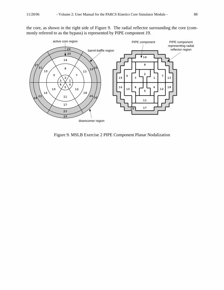
11/28/06 - Volume 2: User Manual for the PARCS Kinetics Core Simulator Module - 88
the core, as shown in the right side of Figure 9. The radial reflector surrounding the core (com-monly referred to as the bypass) is represented by PIPE component 19.
Figure 9. MSLB Exercise 2 PIPE Component Planar Nodalization
1
8
14
23
4 65
79
10
11
12
1315
16
17
18
19
PIPE component PIPE componentrepresenting radial
reflector region
active core region
barrel-baffle region
downcomer region
12
34
56
7
8
9
10
11
12
13
14
15
16
17
18
19
20
23
21
22 24
25
26
27
28
29
30

11/28/06 - Volume 2: User Manual for the PARCS Kinetics Core Simulator Module - 89
The core heat structure nodalization for this exercise consists of 193 heat structure compo-nents. Each of the 177 fuel assemblies in the core is represented by its own heat structure, asshown in Figure 10.
Figure 10. MSLB Exercise 2 HTSTR Component Planar Nodalization
For analysis purposes, the core was divided into six (6) azimuthal sectors, the boundaries ofwhich split the core along its x-axis of symmetry. The layout of the azimuthal sectors fromFigure 6 is reflected in the layout of the PIPE boundaries shown in Figure 9. It was decided thatthe heat structures split by these azimuthal sector boundaries would be divided into two (2) sepa-rate heat structures, each representing half the fuel pins making up the entire assembly. This mod-elling decision made the addition of 15 heat structure components to the TRACE modelnecessary. Finally, the entire radial reflector was represented with a single heat structure compo-nent for consistency with the thermal-hydraulic nodalization, bringing the total number of heatstructures in this model to 193 (177+15+1=193).
The axial nodalization of the heat structure components is identical to that of the PIPE com-ponents to which they are coupled for the active core region, i.e., six (6) axial levels of 59.52 cm
HTSTR componentHTSTR componentrepresenting radial
reflector region
active core region
barrel-baffle region
downcomer region
12
34
56
7
8
9
10
11
12
13
14
15
16
17
18
19
20
23
21
22 24
25
26
27
28
29
30

11/28/06 - Volume 2: User Manual for the PARCS Kinetics Core Simulator Module - 90
each, illustrated in Figure 11. The axial reflector regions (both top and bottom) are lumped intothe top-most and bottom-most axial levels of the heat structures.
Figure 11. MSLB Exercise 2 HTSTR Axial Nodalization
Exercise 2 and 3 PARCS Nodalization
The neutronics nodalization of the MSLB Benchmark consists of 177 fuel assemblies, with eachfuel assembly represented by a single neutronic node. Figure 12 shows the arrangement of theneutronic nodes for each axial plane of the neutronic model.
Figure 12. MSLB Exercise 2 and 3 Neutronic Radial Nodalization
59.52 cm
HTSTR (ROD) component
active coreregion
active fuel node reflector node

11/28/06 - Volume 2: User Manual for the PARCS Kinetics Core Simulator Module - 91
Surrounding the fuel nodes, along the periphery of the core, is a shroud of 64 radial reflectornodes, which represent the flow passing directly through the “bypass” region of the core. Theaxial nodalization of the neutronic model, shown in Figure 13, is somewhat irregular but complieswith the benchmark specifications.
Figure 13. MSLB Exercise 2 and 3 Neutronic Axial Nodalization
A total of 28 axial levels make up the neutronic nodalization, with heights of (from the bot-tom of the core) 21.811 cm, 14.88 cm, 4.71 cm, 10.17 cm, (20*)14.88 cm, 12.266 cm, 2.614 cm,14.88 cm, and 21.811 cm. The top and bottom axial levels represent the axial reflector region.The same nodalization was used for both exercises 2 and 3 of the MSLB benchmark problem.
V.B.3 Explicit Weight Generation
The specification of individual weights for mapping thermal-hydraulic and neutronic spatialdomains is through the use of the %TABLE1 and %TABLE2 cards in the mapping information file.The name of this file is specified on the CNTL card in the PARCS input deck. Each line withinthese tables contains the weighting factor used for mapping a neutronic node to a component inthe TRACE input deck (for both thermal-hydraulic and heat structure components). It is theresponsibility of the user to calculate the mapping weights for these tables, taking into accountboth the radial and axial nodalizations of the thermal-hydraulic and neutronic models and themanner in which they “fit” together. Due to the repetitive nature of explicit weight generation, itis generally easier to split the generation of weights into two separate phases when constructingthem manually. The first phase is to determine the radial weights required for mapping the ther-mal-hydraulic and neutronic spatial domains onto one another. Both thermal-hydraulic and neu-tronic models typically use the same radial nodalization for each axial level in the model.Therefore, the radial weights will usually be the same throughout the models. The second phaseis to calculate the axial weights required for aligning the thermal-hydraulic and neutronic nodal-izations. Like the radial nodalizations, it is typical for the axial nodalization of both thermal-hydraulic and neutronic models to be uniform. Therefore, once the axial weighting factors aredetermined, they are likely to be valid throughout the models. Once both the radial and axial
active coreregion
axial reflector
axial reflector
14.88 cm
21.811 cm

11/28/06 - Volume 2: User Manual for the PARCS Kinetics Core Simulator Module - 92
weighting factors have been determined, the entire set of mapping weights is constructed by mul-tiplying each radial weight by each axial weight.
Determination of the weights must be performed for both thermal-hydraulic (%TABLE1) andheat structure (%TABLE2) components. The suggested procedure for calculating both the radialand axial weights is outlined below using the second exercise of the MSLB benchmark problemas a working example.
Radial Weight Generation
The generation of the radial weights is often little more than determining (visually) whereneutronic nodes fall within the thermal-hydraulic and heat structure nodalization.
Thermal-Hydraulic to Neutronic Radial Weight Generation
For this purpose, Figure 9 and Figure 12 are shown overlayed below. From Figure 14, it canbe visually determined that most neutronic nodes fall completely within the boundaries repre-sented by a single thermal-hydraulic PIPE component. For example, PIPE number 8 representsthe coolant flow for all 10 neutronic nodes within the confines of its boldface box. For instruc-tional purposes, the 10 neutronic nodes linked to PIPE component 8 are shown in dark grey inFigure 14. The radial weight for each of the neutronic nodes contained within PIPE 8 is 1.0. Infact, all the radial weights are 1.0, with the exception of those corresponding to the neutronicnodes along the x-axis of symmetry.
Figure 14. Radial Mapping Visualization for Exercise 2 of MSLB
Each of the neutronic nodes along the x-axis of symmetry is contained by two adjacent PIPEcomponents. Because half of the each neutronic node exists in each of the two PIPE components,each neutronic node along this boundary has a radial weight of 0.5 for each PIPE component towhich it is coupled. The sum of the radial weights for each neutronic node must be 1.0. In this
1
8
14
23
4 65
79
10
11
12
1315
16
17
18
19
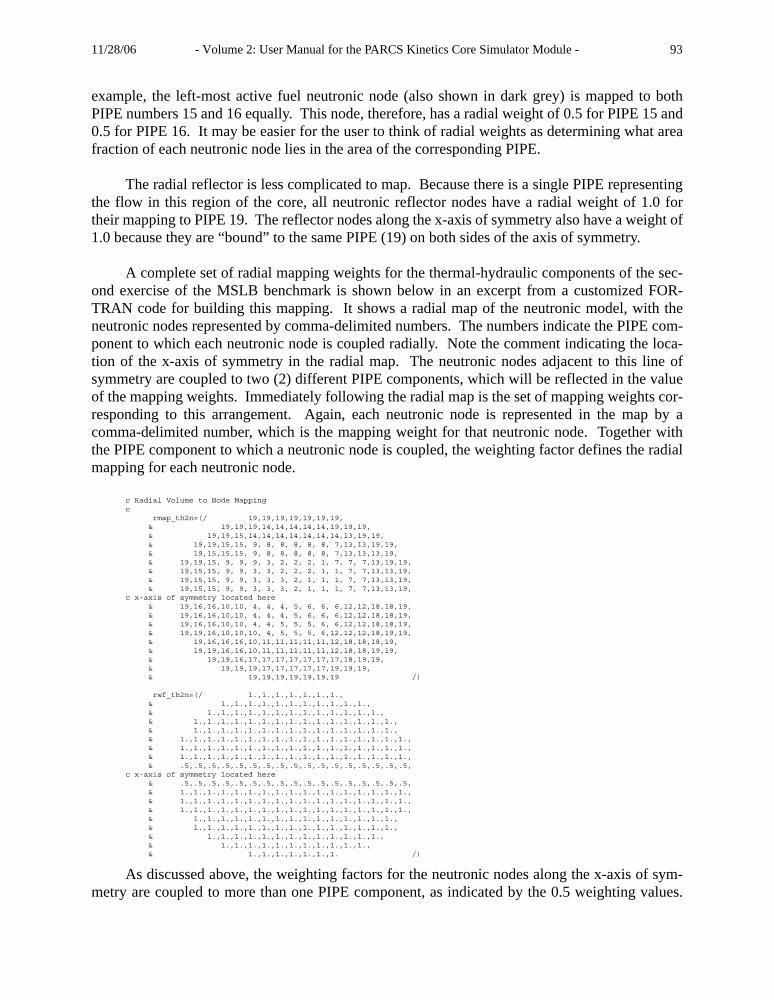
11/28/06 - Volume 2: User Manual for the PARCS Kinetics Core Simulator Module - 93
example, the left-most active fuel neutronic node (also shown in dark grey) is mapped to bothPIPE numbers 15 and 16 equally. This node, therefore, has a radial weight of 0.5 for PIPE 15 and0.5 for PIPE 16. It may be easier for the user to think of radial weights as determining what areafraction of each neutronic node lies in the area of the corresponding PIPE.
The radial reflector is less complicated to map. Because there is a single PIPE representingthe flow in this region of the core, all neutronic reflector nodes have a radial weight of 1.0 fortheir mapping to PIPE 19. The reflector nodes along the x-axis of symmetry also have a weight of1.0 because they are “bound” to the same PIPE (19) on both sides of the axis of symmetry.
A complete set of radial mapping weights for the thermal-hydraulic components of the sec-ond exercise of the MSLB benchmark is shown below in an excerpt from a customized FOR-TRAN code for building this mapping. It shows a radial map of the neutronic model, with theneutronic nodes represented by comma-delimited numbers. The numbers indicate the PIPE com-ponent to which each neutronic node is coupled radially. Note the comment indicating the loca-tion of the x-axis of symmetry in the radial map. The neutronic nodes adjacent to this line ofsymmetry are coupled to two (2) different PIPE components, which will be reflected in the valueof the mapping weights. Immediately following the radial map is the set of mapping weights cor-responding to this arrangement. Again, each neutronic node is represented in the map by acomma-delimited number, which is the mapping weight for that neutronic node. Together withthe PIPE component to which a neutronic node is coupled, the weighting factor defines the radialmapping for each neutronic node.
c Radial Volume to Node Mappingc rmap_th2n=(/ 19,19,19,19,19,19,19, & 19,19,19,14,14,14,14,14,19,19,19, & 19,19,15,14,14,14,14,14,14,14,13,19,19, & 19,19,15,15, 9, 8, 8, 8, 8, 8, 7,13,13,19,19, & 19,15,15,15, 9, 8, 8, 8, 8, 8, 7,13,13,13,19, & 19,19,15, 9, 9, 9, 3, 2, 2, 2, 1, 7, 7, 7,13,19,19, & 19,15,15, 9, 9, 3, 3, 2, 2, 2, 1, 1, 7, 7,13,13,19, & 19,15,15, 9, 9, 3, 3, 3, 2, 1, 1, 1, 7, 7,13,13,19, & 19,15,15, 9, 9, 3, 3, 3, 2, 1, 1, 1, 7, 7,13,13,19,c x-axis of symmetry located here & 19,16,16,10,10, 4, 4, 4, 5, 6, 6, 6,12,12,18,18,19, & 19,16,16,10,10, 4, 4, 4, 5, 6, 6, 6,12,12,18,18,19, & 19,16,16,10,10, 4, 4, 5, 5, 5, 6, 6,12,12,18,18,19, & 19,19,16,10,10,10, 4, 5, 5, 5, 6,12,12,12,18,19,19, & 19,16,16,16,10,11,11,11,11,11,12,18,18,18,19, & 19,19,16,16,10,11,11,11,11,11,12,18,18,19,19, & 19,19,16,17,17,17,17,17,17,17,18,19,19, & 19,19,19,17,17,17,17,17,19,19,19, & 19,19,19,19,19,19,19 /)
rwf_th2n=(/ 1.,1.,1.,1.,1.,1.,1., & 1.,1.,1.,1.,1.,1.,1.,1.,1.,1.,1., & 1.,1.,1.,1.,1.,1.,1.,1.,1.,1.,1.,1.,1., & 1.,1.,1.,1.,1.,1.,1.,1.,1.,1.,1.,1.,1.,1.,1., & 1.,1.,1.,1.,1.,1.,1.,1.,1.,1.,1.,1.,1.,1.,1., & 1.,1.,1.,1.,1.,1.,1.,1.,1.,1.,1.,1.,1.,1.,1.,1.,1., & 1.,1.,1.,1.,1.,1.,1.,1.,1.,1.,1.,1.,1.,1.,1.,1.,1., & 1.,1.,1.,1.,1.,1.,1.,1.,1.,1.,1.,1.,1.,1.,1.,1.,1., & .5,.5,.5,.5,.5,.5,.5,.5,.5,.5,.5,.5,.5,.5,.5,.5,.5,c x-axis of symmetry located here & .5,.5,.5,.5,.5,.5,.5,.5,.5,.5,.5,.5,.5,.5,.5,.5,.5, & 1.,1.,1.,1.,1.,1.,1.,1.,1.,1.,1.,1.,1.,1.,1.,1.,1., & 1.,1.,1.,1.,1.,1.,1.,1.,1.,1.,1.,1.,1.,1.,1.,1.,1., & 1.,1.,1.,1.,1.,1.,1.,1.,1.,1.,1.,1.,1.,1.,1.,1.,1., & 1.,1.,1.,1.,1.,1.,1.,1.,1.,1.,1.,1.,1.,1.,1., & 1.,1.,1.,1.,1.,1.,1.,1.,1.,1.,1.,1.,1.,1.,1., & 1.,1.,1.,1.,1.,1.,1.,1.,1.,1.,1.,1.,1., & 1.,1.,1.,1.,1.,1.,1.,1.,1.,1.,1., & 1.,1.,1.,1.,1.,1.,1. /)
As discussed above, the weighting factors for the neutronic nodes along the x-axis of sym-metry are coupled to more than one PIPE component, as indicated by the 0.5 weighting values.
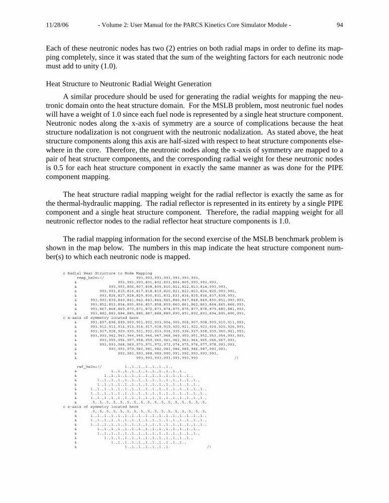
11/28/06 - Volume 2: User Manual for the PARCS Kinetics Core Simulator Module - 94
Each of these neutronic nodes has two (2) entries on both radial maps in order to define its map-ping completely, since it was stated that the sum of the weighting factors for each neutronic nodemust add to unity (1.0).
Heat Structure to Neutronic Radial Weight Generation
A similar procedure should be used for generating the radial weights for mapping the neu-tronic domain onto the heat structure domain. For the MSLB problem, most neutronic fuel nodeswill have a weight of 1.0 since each fuel node is represented by a single heat structure component.Neutronic nodes along the x-axis of symmetry are a source of complications because the heatstructure nodalization is not congruent with the neutronic nodalization. As stated above, the heatstructure components along this axis are half-sized with respect to heat structure components else-where in the core. Therefore, the neutronic nodes along the x-axis of symmetry are mapped to apair of heat structure components, and the corresponding radial weight for these neutronic nodesis 0.5 for each heat structure component in exactly the same manner as was done for the PIPEcomponent mapping.
The heat structure radial mapping weight for the radial reflector is exactly the same as forthe thermal-hydraulic mapping. The radial reflector is represented in its entirety by a single PIPEcomponent and a single heat structure component. Therefore, the radial mapping weight for allneutronic reflector nodes to the radial reflector heat structure components is 1.0.
The radial mapping information for the second exercise of the MSLB benchmark problem isshown in the map below. The numbers in this map indicate the heat structure component num-ber(s) to which each neutronic node is mapped.
c Radial Heat Structure to Node Mapping rmap_hs2n=(/ 993,993,993,993,993,993,993, & 993,993,993,801,802,803,804,805,993,993,993, & 993,993,806,807,808,809,810,811,812,813,814,993,993, & 993,993,815,816,817,818,819,820,821,822,823,824,825,993,993, & 993,826,827,828,829,830,831,832,833,834,835,836,837,838,993, & 993,993,839,840,841,842,843,844,845,846,847,848,849,850,851,993,993, & 993,852,853,854,855,856,857,858,859,860,861,862,863,864,865,866,993, & 993,867,868,869,870,871,872,873,874,875,876,877,878,879,880,881,993, & 993,882,883,884,885,886,887,888,889,890,891,892,893,894,895,896,993,c x-axis of symmetry located here & 993,897,898,899,900,901,902,903,904,905,906,907,908,909,910,911,993, & 993,912,913,914,915,916,917,918,919,920,921,922,923,924,925,926,993, & 993,927,928,929,930,931,932,933,934,935,936,937,938,939,940,941,993, & 993,993,942,943,944,945,946,947,948,949,950,951,952,953,954,993,993, & 993,955,956,957,958,959,960,961,962,963,964,965,966,967,993, & 993,993,968,969,970,971,972,973,974,975,976,977,978,993,993, & 993,993,979,980,981,982,983,984,985,986,987,993,993, & 993,993,993,988,989,990,991,992,993,993,993, & 993,993,993,993,993,993,993 /)
rwf_hs2n=(/ 1.,1.,1.,1.,1.,1.,1., & 1.,1.,1.,1.,1.,1.,1.,1.,1.,1.,1., & 1.,1.,1.,1.,1.,1.,1.,1.,1.,1.,1.,1.,1., & 1.,1.,1.,1.,1.,1.,1.,1.,1.,1.,1.,1.,1.,1.,1., & 1.,1.,1.,1.,1.,1.,1.,1.,1.,1.,1.,1.,1.,1.,1., & 1.,1.,1.,1.,1.,1.,1.,1.,1.,1.,1.,1.,1.,1.,1.,1.,1., & 1.,1.,1.,1.,1.,1.,1.,1.,1.,1.,1.,1.,1.,1.,1.,1.,1., & 1.,1.,1.,1.,1.,1.,1.,1.,1.,1.,1.,1.,1.,1.,1.,1.,1., & .5,.5,.5,.5,.5,.5,.5,.5,.5,.5,.5,.5,.5,.5,.5,.5,.5,c x-axis of symmetry located here & .5,.5,.5,.5,.5,.5,.5,.5,.5,.5,.5,.5,.5,.5,.5,.5,.5, & 1.,1.,1.,1.,1.,1.,1.,1.,1.,1.,1.,1.,1.,1.,1.,1.,1., & 1.,1.,1.,1.,1.,1.,1.,1.,1.,1.,1.,1.,1.,1.,1.,1.,1., & 1.,1.,1.,1.,1.,1.,1.,1.,1.,1.,1.,1.,1.,1.,1.,1.,1., & 1.,1.,1.,1.,1.,1.,1.,1.,1.,1.,1.,1.,1.,1.,1., & 1.,1.,1.,1.,1.,1.,1.,1.,1.,1.,1.,1.,1.,1.,1., & 1.,1.,1.,1.,1.,1.,1.,1.,1.,1.,1.,1.,1., & 1.,1.,1.,1.,1.,1.,1.,1.,1.,1.,1., & 1.,1.,1.,1.,1.,1.,1. /)

11/28/06 - Volume 2: User Manual for the PARCS Kinetics Core Simulator Module - 95
The values of the weights for defining the mapping between the heat structure components andthe neutronic nodes are the same as were defined for the mapping of the thermal-hydraulic com-ponents. Just as each neutronic node along the x-axis of symmetry was coupled to two (2) PIPEcomponents, each node along this axis is also coupled to two (2) heat structure components. Forthis reason, the mapping weights for both thermal-hydraulic and heat structure components areidentical. This can be seen in the listing of the mapping weights themselves.
Axial Weight Generation
Determination of the axial weights uses a procedure similar to the generation of the radialmapping weights. However, it is not unusual for the thermal-hydraulic, heat structure, and neu-tronic nodalizations to differ completely in the axial direction. In most cases, uniform axialweights are used throughout the entire core, i.e., every neutronic node uses the same axial weightsince the axial nodalization is typically uniform throughout the core. Because this is the case, anysmall error in the axial weights is propagated throughout the entire core with little indication ofanything wrong.
The weights generated for the mapping of the thermal-hydraulic and heat structure nodaliza-tions onto the neutronic nodalization are two-way. The weights that determine how thermal-hydraulic and heat structure component properties factor into reactivity feedback in the neutronicscalculation are also used for determining how neutronic power is distributed throughout both ther-mal-hydraulic and heat structure components.
The thermal-hydraulic properties required to calculate feedback within PARCS are cell-centeredor cell-averaged quantities: liquid temperature, liquid and vapor densities, void fraction, andboron concentration. The properties obtained from heat structure components -- volume-aver-aged fuel temperature, fuel centerline temperature, and fuel surface temperature -- are also cell-centered quantities. Finally, the power calculated by PARCS is calculated at the center of eachneutronic node. Since all quantities are represented at the center of their respective volumes/nodes, the calculation of the axial weights is mainly a task of determining how the centers of thethermal-hydraulic and heat structure component cells align with the centers of the neutronicnodes. The suggested procedure for resolving the axial mapping weights is described below.
Thermal-Hydraulic to Neutronic Axial Weight Generation
Figure 15 below shows the axial nodalization of the PIPE components for the second exer-cise of the MSLB benchmark problem aligned with the neutronic nodalization. The PIPE cellsnumbers are indicated in the center of each cell, while the neutronic axial node is along the right

11/28/06 - Volume 2: User Manual for the PARCS Kinetics Core Simulator Module - 96
side of the neutronic nodalization. Note that for brevity, not every axial node in the neutronicmodel is labelled.
Figure 15. Axial Alignment of MSLB Exercise 2 Thermal-Hydraulic and Neutronic Models
It can be seen from Figure 15 that the bottom reflector neutronic node is mapped to cell 1 of thePIPE component, as was described in Section above. Since the nodalization of the neutronicsmodel was provided in the MSLB benchmark specifications, there is a mis-match of neutronicand thermal-hydraulic node volumes for the axial reflector nodes. This inaccuracy does not intro-duce any error, as the nodalization makes these neutronic nodes of sufficient thickness to be con-sidered infinite reflectors. Therefore, increasing their volume to match that of their respectivethermal-hydraulic node will have no impact on the solution. Neutronic axial levels 2 through 6
1
2
3
4
5
6
7
8
1
5
10
15
20
25
28
PIPE PARCS
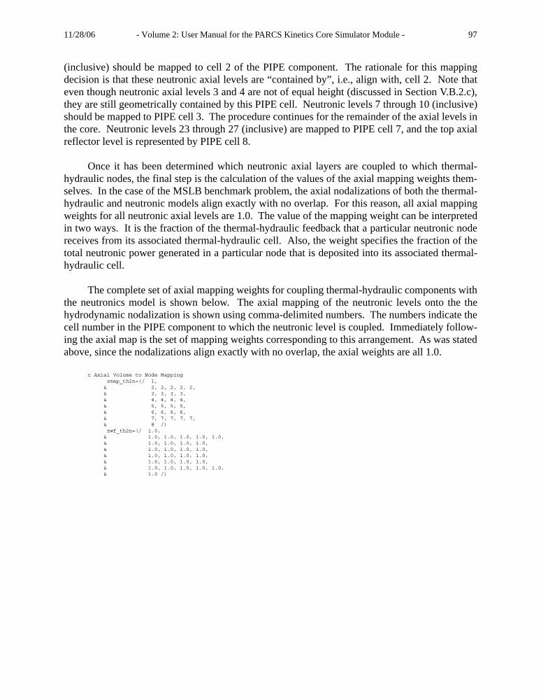
11/28/06 - Volume 2: User Manual for the PARCS Kinetics Core Simulator Module - 97
(inclusive) should be mapped to cell 2 of the PIPE component. The rationale for this mappingdecision is that these neutronic axial levels are “contained by”, i.e., align with, cell 2. Note thateven though neutronic axial levels 3 and 4 are not of equal height (discussed in Section V.B.2.c),they are still geometrically contained by this PIPE cell. Neutronic levels 7 through 10 (inclusive)should be mapped to PIPE cell 3. The procedure continues for the remainder of the axial levels inthe core. Neutronic levels 23 through 27 (inclusive) are mapped to PIPE cell 7, and the top axialreflector level is represented by PIPE cell 8.
Once it has been determined which neutronic axial layers are coupled to which thermal-hydraulic nodes, the final step is the calculation of the values of the axial mapping weights them-selves. In the case of the MSLB benchmark problem, the axial nodalizations of both the thermal-hydraulic and neutronic models align exactly with no overlap. For this reason, all axial mappingweights for all neutronic axial levels are 1.0. The value of the mapping weight can be interpretedin two ways. It is the fraction of the thermal-hydraulic feedback that a particular neutronic nodereceives from its associated thermal-hydraulic cell. Also, the weight specifies the fraction of thetotal neutronic power generated in a particular node that is deposited into its associated thermal-hydraulic cell.
The complete set of axial mapping weights for coupling thermal-hydraulic components withthe neutronics model is shown below. The axial mapping of the neutronic levels onto the thehydrodynamic nodalization is shown using comma-delimited numbers. The numbers indicate thecell number in the PIPE component to which the neutronic level is coupled. Immediately follow-ing the axial map is the set of mapping weights corresponding to this arrangement. As was statedabove, since the nodalizations align exactly with no overlap, the axial weights are all 1.0.
c Axial Volume to Node Mapping zmap_th2n=(/ 1, & 2, 2, 2, 2, 2, & 3, 3, 3, 3, & 4, 4, 4, 4, & 5, 5, 5, 5, & 6, 6, 6, 6, & 7, 7, 7, 7, 7, & 8 /) zwf_th2n=(/ 1.0, & 1.0, 1.0, 1.0, 1.0, 1.0, & 1.0, 1.0, 1.0, 1.0, & 1.0, 1.0, 1.0, 1.0, & 1.0, 1.0, 1.0, 1.0, & 1.0, 1.0, 1.0, 1.0, & 1.0, 1.0, 1.0, 1.0, 1.0, & 1.0 /)
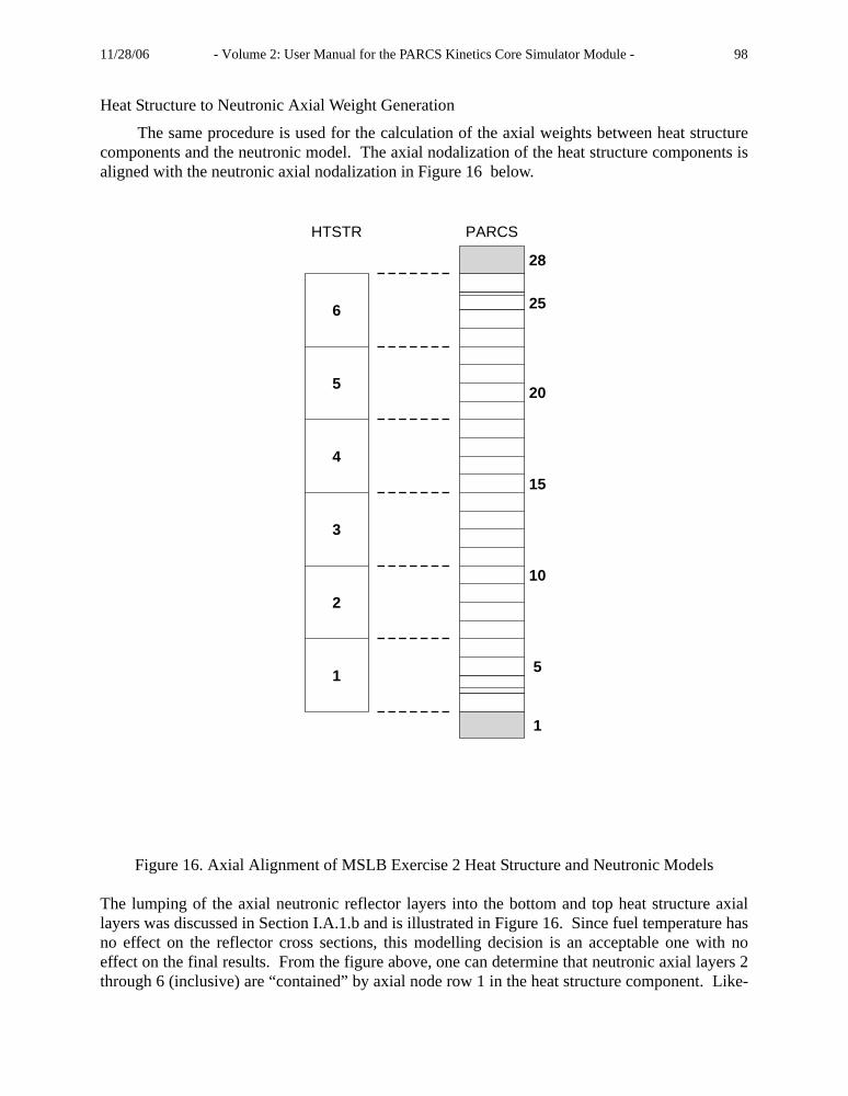
11/28/06 - Volume 2: User Manual for the PARCS Kinetics Core Simulator Module - 98
Heat Structure to Neutronic Axial Weight Generation
The same procedure is used for the calculation of the axial weights between heat structurecomponents and the neutronic model. The axial nodalization of the heat structure components isaligned with the neutronic axial nodalization in Figure 16 below.
Figure 16. Axial Alignment of MSLB Exercise 2 Heat Structure and Neutronic Models
The lumping of the axial neutronic reflector layers into the bottom and top heat structure axiallayers was discussed in Section I.A.1.b and is illustrated in Figure 16. Since fuel temperature hasno effect on the reflector cross sections, this modelling decision is an acceptable one with noeffect on the final results. From the figure above, one can determine that neutronic axial layers 2through 6 (inclusive) are “contained” by axial node row 1 in the heat structure component. Like-
HTSTR
1
2
3
4
5
6
1
5
10
15
20
25
28
PARCS

11/28/06 - Volume 2: User Manual for the PARCS Kinetics Core Simulator Module - 99
wise, neutronic layers 7 through 10 (inclusive) are coupled to heat structure axial node row 2.The remainder of the heat structure to neutronic mapping uses the same procedure as was detailedabove in the thermal-hydraulic to neutronic mapping in Section .
The complete set of axial mapping weights for coupling the neutronic and heat structurenodalizations is shown below, using the same format as for the hydrodynamic axial mappingweights. As was stated above, the top and bottom axial reflectors were not explicitly modelled bya heat structure node. These neutronic reflector nodes were lumped into the top- and bottom-mostheat structure nodes, as can be observed in the mapping below.
c Axial Heat Structure to Node Mapping zmap_hs2n=(/ 1, & 1, 1, 1, 1, 1, & 2, 2, 2, 2, & 3, 3, 3, 3, & 4, 4, 4, 4, & 5, 5, 5, 5, & 6, 6, 6, 6, 6, & 6 /) zwf_hs2n=(/ 1.0, & 1.0, 1.0, 1.0, 1.0, 1.0, & 1.0, 1.0, 1.0, 1.0, & 1.0, 1.0, 1.0, 1.0, & 1.0, 1.0, 1.0, 1.0, & 1.0, 1.0, 1.0, 1.0, & 1.0, 1.0, 1.0, 1.0, 1.0, & 1.0 /)
Putting It All Together
Once the radial and axial weights have been generated for both the hydrodynamic- and heatstructure-to-neutronic mesh mapping, the final task is to construct a list of the exact mappingweights between each neutronic node and its coupled hydrodynamic and heat structure compo-nents. The %TABLE1 and %TABLE2 cards are used in the mapping input file for specifying themapping weights for hydrodynamic and heat structure components, respectively.
%TABLE1 Card
This card relates to the mapping between hydrodynamic volumes and neutronic nodes.Each line of data which follows this card is read in free format and contains five (5) numbers perrow (integer, integer, integer, integer, real) corresponding to:
Integer #1: TRACE Hydraulic Component Number
This value should correspond to that specified by the user in the TRACEinput deck for the specific component (e.g. vessel, chan, or pipe).
Integer #2: Component Cell Number
For the vessel component, this number should correspond to the radial cellnumber in the T/H plane. For chan or pipe components this number shouldcorrespond to the cell number within the chan or pipe.
Integer #3: Component Axial Level
For the vessel component, this number is the axial plane number. For chanor pipe components, this number should be “0”.

11/28/06 - Volume 2: User Manual for the PARCS Kinetics Core Simulator Module - 100
Integer #4: PARCS Node Number
Real #1: Weighting Factor
The sum of the input weighting factors for a particular PARCS node num-ber should be equal to 1.0.
The weighting factor is determined from the product of the corresponding radial and axialweights for the particular hydrodynamic volume and neutronic node in question.
Example:%TABLE1 51 1 0 1 1.0000 51 1 0 2 0.5000 52 1 0 2 0.5000 52 1 0 3 1.0000
%TABLE2 Card
This card relates to the mapping between heat structures and neutronic nodes. Each line ofdata which follows this card is read in free format and contains five numbers per row (integer,integer, integer, integer, real) corresponding to:
Integer #1: TRACE Heat Structure Component Number
This value should correspond to that specified by the user in the TRACEinput deck for the specific component (e.g. rod, slab, htstr, or chan).
Integer #2: HS Average ROD/SLAB/HTSTR Number
This value is the rod group number for the heat structure component speci-fied in the first integer field.
Integer #3: Component Axial Level
This value is the axial level within the heat structure rod specified by thefirst two integer fields.
Integer #4: PARCS Node Number
Real #1: Weighting Factor
The sum of the input weighting factors for a particular PARCS node num-ber should either be equal to 1.0 or 0.0. If the sum is equal to 0.0 for anyPARCS node, then it is assumed that this node is not connected to any heatstructure.
Note: The PARCS node numbers to be used in TABLE1 and TABLE2 should be consistent withthose used in the PARCS code, which utilizes a plane ordering, as shown below:

11/28/06 - Volume 2: User Manual for the PARCS Kinetics Core Simulator Module - 101
where,
and L corresponds to the number of nodes in a plane and K corresponds to the number of planes.
Example:%TABLE2 51 1 1 1 1.0000 51 1 1 2 0.5000 52 1 1 2 0.5000 52 1 1 3 1.0000
V.B.4 VOLRMAP1 Card
This card specifies the type of component to which PARCS is coupled (e.g. vessel or chan).If "vessel" is input, the 2nd word must be the vessel component number. If "chan" is input, nocomponent number should follow. The component numbers for chans will be taken fromVOLRMAP2.
Example:%VOLRMAP1chan
V.B.5 VOLRMAP2 Cards
These cards specify the radial cell numbers to be coupled to each PARCS radial node. Forvessel components, these numbers are the relative cell numbers in the r-theta (or x-y) plane. Forchan components, these numbers are the actual chan number. The format of the map is as follows:
(1) The first row (line) of the map must contain a "0" in the first column followed by thenumbers which relate to the column index in the neutronic plane.
(2) In each line that follows, the first column contains the row number for the neutronicplane, followed by the mapped cell numbers. NOTE: place holders (for non-node loca-tions) are input using any character besides 0-9.
(3) Secondary maps can be entered, and will be detected when the first column of a pro-cessed line contains a "0" (indicating that column indices are to be read from this line).
Example:%VOLRMAP20 1 2 2 31 51 51 52 522 51 51 52 522 53 53 54 54
Node Ordering N11 … NL
1 … N1K … NL
K=
Nlk k 1–( ) L l+×( )= l 1 2 …L k;, , 1 2…K,= =( )

11/28/06 - Volume 2: User Manual for the PARCS Kinetics Core Simulator Module - 102
3 53 53 54 54
V.B.6 VOLRMAP3 CardsThese cards specify the radial weighting factors for the map input with the
VOLRMAP2 cards. The input format for these cards is the same as that for VOLRMAP2. It isnecessary that the input radial form of VOLRMAP2 and VOLRMAP3 match exactly. The firstline of these cards is the same as the first line of the VOLRMAP2 cards.
Example:%VOLRMAP30 1 2 2 31 1.0 0.5 0.5 1.02 0.5 0.25 0.25 0.52 0.5 0.25 0.25 0.53 1.0 0.5 0.5 1.0
V.B.7 DOPL CardThis card specifies the option for calculating the Doppler fuel temperature feedback.
Either the volume average fuel temperature or a linear combination of the fuel centerline and sur-face temperatures can be used for calculating the effective temperature. The volume-averagedfuel temperature is specified using AVG on the DOPL Card and the linear method is specifiedusing LINC on the DOPL Card, where the parameter specifies the weighting of the fuel cen-terline, , and fuel surface temperature, :
,
A default of is used for cylindrical fuel pins. When specifying the linear combinationoption, the weighting factor, , must also be provided on the card. Use of the average fuel tem-perature option requires no such option.
Examples:%DOPL LINC 0.7
%DOPLAVG
V.B.8 TRIP CardThis card specifies which TRACE control system trip ID will be used for signaling reactor
scram and requires only the integer ID number of the trip in the TRACE model to be monitoredfor scram simulation.
Example:
ω
Tf0 Tf
s
TDopl 1 ω–( )Tf0 ωTf
s+=
ω 0.7=ω

11/28/06 - Volume 2: User Manual for the PARCS Kinetics Core Simulator Module - 103
%TRIP 2
V.B.9 MAPTAB ExamplesThree examples of MAPTAB input are shown below for the same 2-D mapping scheme. The
first two examples demonstrate the use of the VOLRMAP series, and the third example demon-strates the use of the TABLE series. For the VOLRMAP series, the first example uses one radialmap each for VOLRMAP2 and VOLRMAP3 to specify the T/H to neutronic mapping. The sec-ond example uses 4 radial maps each for VOLRMAP2 and VOLRMAP3 to input the same map-ping. Note the use of the asterisk (“*”) character as a placeholder in VOLRMAP2 andVOLRMAP3 in example 2, which indicates no additional mapping information is provided forthe corresponding neutronic node.
Example #1:** Method of Calculating Doppler Temperature* LINC: Linear Combination (requires weighting factor)* AVG: Average Temperature*%DOPL* LINC 0.7 AVG** Trip Unit Number for TRACE*%TRIP 2%VOLRMAP1chan%VOLRMAP20 1 2 2 31 51 51 52 522 51 51 52 522 53 53 54 543 53 53 54 54%VOLRMAP30 1 2 2 31 1.0 0.5 0.5 1.02 0.5 0.25 0.25 0.52 0.5 0.25 0.25 0.53 1.0 0.5 0.5 1.0
Example #2:** Method of Calculating Doppler Temperature

11/28/06 - Volume 2: User Manual for the PARCS Kinetics Core Simulator Module - 104
* LINC: Linear Combination (requires weighting factor)* AVG: Average Temperature*%DOPL* LINC 0.7 AVG** Trip Unit Number for TRACE*%TRIP 2%VOLRMAP1 chan%VOLRMAP20 1 2 31 51 51 522 51 51 523 53 53 54*0 1 2 31 * 52 *2 53 52 543 * 53 **0 1 2 31 * * *2 * 53 *3 * * **0 1 2 31 * * *2 * 54 *3 * * *%VOLRMAP30 1 2 31 1.0 0.5 1.02 0.5 0.25 0.253 1.0 0.5 1.0*0 1 2 31 * 0.5 *2 0.5 0.25 0.53 * 0.5 **0 1 2 31 * * *2 * 0.25 *3 * * **0 1 2 3

11/28/06 - Volume 2: User Manual for the PARCS Kinetics Core Simulator Module - 105
1 * * *2 * 0.25 *3 * * *
Example #3:** Method of Calculating Doppler Temperature* LINC: Linear Combination (requires weighting factor)* AVG: Average Temperature*%DOPL* LINC 0.7 AVG** Trip Unit Number for TRACE*%TRIP 2** Volume to Node Table*%TABLE1 51 1 0 1 1.0000 51 1 0 2 0.5000 52 1 0 2 0.5000 52 1 0 3 1.0000 51 1 0 4 0.5000 53 1 0 4 0.5000 51 1 0 5 0.2500 52 1 0 5 0.2500 53 1 0 5 0.2500 54 1 0 5 0.2500 52 1 0 6 0.5000 54 1 0 6 0.5000 53 1 0 7 1.0000 53 1 0 8 0.5000 54 1 0 8 0.5000 54 1 0 9 1.0000** Heat Structure to Node Table*%TABLE2 51 1 1 1 1.0000 51 1 1 2 0.5000 52 1 1 2 0.5000 52 1 1 3 1.0000 51 1 1 4 0.5000
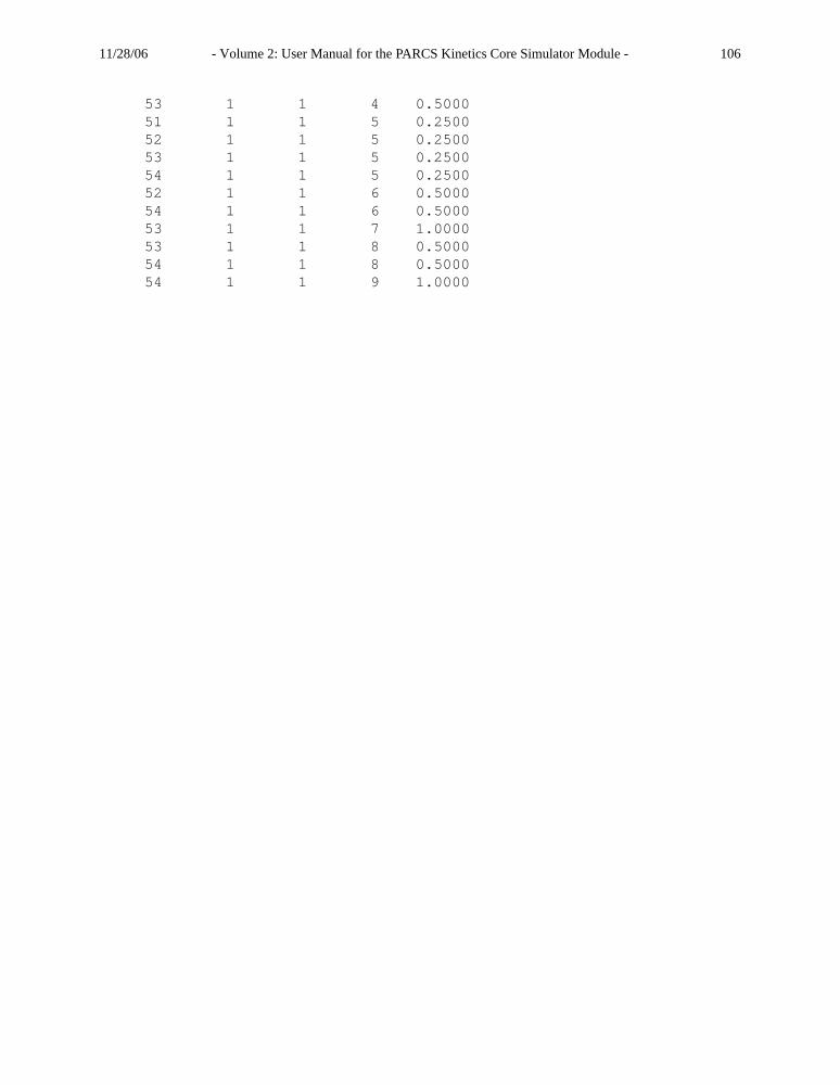
11/28/06 - Volume 2: User Manual for the PARCS Kinetics Core Simulator Module - 106
53 1 1 4 0.5000 51 1 1 5 0.2500 52 1 1 5 0.2500 53 1 1 5 0.2500 54 1 1 5 0.2500 52 1 1 6 0.5000 54 1 1 6 0.5000 53 1 1 7 1.0000 53 1 1 8 0.5000 54 1 1 8 0.5000 54 1 1 9 1.0000

11/28/06 - Volume 2: User Manual for the PARCS Kinetics Core Simulator Module - 107
VI. SAMPLE INPUTS
VI.A OECD MSLB Benchmark
VI.A.1 Steady State Input Deck
CASEID ss OECD/NEA MSLB !****************************************************************************** CNTL ext_th T ../rad.map TRAC 50 core_power 100.0 bank_pos 971.0 971.0 971.0 971.0 971.0 971.0 900.0 971.0 pin_power F! input iteration planar adj! edit table power pin reac! print_opt T F T F T print_opt F F F F F! fdbk flux planar! rho precurs flux Xe T/H print_opt F F F F F !******************************************************************************XSEC func_type 11 dnp_ngrp 6 dhp_beta 2.35402E-02 1.89077E-02 1.39236E-02 6.90315E-03 3.56888E-03 3.31633E-03 dhp_lambda 1.05345E-01 8.37149E-03 5.20337E-04 4.73479E-05 3.28153E-06 1.17537E-11 kin_comp 1 1 -438 dnp_beta 0.000153 0.001086 0.000965 0.002019 0.000791 0.000197 dnp_lambda 0.012818 0.031430 0.125062 0.329776 1.414748 3.822362 neut_velo 1.83E7 4.01E5 !******************************************************************************GEOM! file ../GEOM_FC! ------------------------------------------------------------------------------ geo_dim 17 17 28 Rad_Conf 0 0 0 0 0 1 1 1 1 1 1 1 0 0 0 0 0 0 0 0 1 1 1 2 2 2 2 2 1 1 1 0 0 0 0 0 1 1 2 2 2 2 2 2 2 2 2 1 1 0 0 0 1 1 2 2 2 2 2 2 2 2 2 2 2 1 1 0 0 1 2 2 2 2 2 2 2 2 2 2 2 2 2 1 0 1 1 2 2 2 2 2 2 2 2 2 2 2 2 2 1 1 1 2 2 2 2 2 2 2 2 2 2 2 2 2 2 2 1 1 2 2 2 2 2 2 2 2 2 2 2 2 2 2 2 1 1 2 2 2 2 2 2 2 2 2 2 2 2 2 2 2 1 1 2 2 2 2 2 2 2 2 2 2 2 2 2 2 2 1 1 2 2 2 2 2 2 2 2 2 2 2 2 2 2 2 1 1 1 2 2 2 2 2 2 2 2 2 2 2 2 2 1 1 0 1 2 2 2 2 2 2 2 2 2 2 2 2 2 1 0 0 1 1 2 2 2 2 2 2 2 2 2 2 2 1 1 0 0 0 1 1 2 2 2 2 2 2 2 2 2 1 1 0 0 0 0 0 1 1 1 2 2 2 2 2 1 1 1 0 0 0

11/28/06 - Volume 2: User Manual for the PARCS Kinetics Core Simulator Module - 108
0 0 0 0 0 1 1 1 1 1 1 1 0 0 0 0 0 grid_x 17*21.811 neutmesh_x 17*1 grid_y 17*21.811 neutmesh_y 17*1 grid_z 21.811 14.88 4.71 10.17 20*14.88 12.266 2.614 14.88 21.811 Boun_cond 1 1 1 1 1 1 Planar_reg 1 24 24 24 24 24 24 24 24 24 24 24 24 24 24 24 24 24 24 24 24 24 24 24 24 24 24 24 24 24 24 24 24 24 24 24 24 24 24 24 24 24 24 24 24 24 24 24 24 24 24 24 24 24 24 24 24 24 24 24 24 24 24 24 24 24 24 24 24 24 24 24 24 24 24 24 24 24 24 24 24 24 24 24 24 24 24 24 24 24 24 24 24 24 24 24 24 24 24 24 24 24 24 24 24 24 24 24 24 24 24 24 24 24 24 24 24 24 24 24 24 24 24 24 24 24 24 24 24 24 24 24 24 24 24 24 24 24 24 24 24 24 24 24 24 24 24 24 24 24 24 24 24 24 24 24 24 24 24 24 24 24 24 24 24 24 24 24 24 24 24 24 24 24 24 24 24 24 24 24 24 24 24 24 24 24 24 24 24 24 24 24 24 24 24 24 24 24 24 24 24 24 24 24 24 24 24 24 24 24 24 24 24 24 24 24 24 24 24 24 24 24 24 24 24 24 24 24 24 24 24 24 24 24 24 24 24 24 24 24 24 24 Planar_reg 2 25 25 25 25 25 25 25 25 25 25 304 214 109 214 304 25 25 25 25 25 409 364 289 199 94 199 289 364 409 25 25 25 25 424 394 349 274 184 79 184 274 349 394 424 25 25 25 409 394 379 334 259 169 64 169 259 334 379 394 409 25 25 25 364 349 334 319 244 154 49 154 244 319 334 349 364 25 25 25 304 289 274 259 244 229 139 34 139 229 244 259 274 289 304 25 25 214 199 184 169 154 139 124 16 124 139 154 169 184 199 214 25 25 109 94 79 64 49 34 16 1 16 34 49 64 79 94 109 25 25 214 199 184 169 154 139 124 16 124 139 154 169 184 199 214 25 25 304 289 274 259 244 229 139 34 139 229 244 259 274 289 304 25 25 25 364 349 334 319 244 154 49 154 244 319 334 349 364 25 25 25 409 394 379 334 259 169 64 169 259 334 379 394 409 25 25 25 424 394 349 274 184 79 184 274 349 394 424 25 25 25 25 409 364 289 199 94 199 289 364 409 25 25 25 25 25 304 214 109 214 304 25 25 25 25 25 25 25 25 25 25...... Planar_reg 16 25 25 25 25 25 25 25 25 25 25 318 228 123 228 318 25 25 25 25 25 423 378 303 213 108 213 303 378 423 25 25 25 25 438 408 363 288 198 93 198 288 363 408 438 25 25 25 423 408 393 348 273 183 78 183 273 348 393 408 423 25 25 25 378 363 348 333 258 168 63 168 258 333 348 363 378 25 25 25 318 303 288 273 258 243 153 48 153 243 258 273 288 303 318 25 25 228 213 198 183 168 153 138 33 138 153 168 183 198 213 228 25 25 123 108 93 78 63 48 33 15 33 48 63 78 93 108 123 25

11/28/06 - Volume 2: User Manual for the PARCS Kinetics Core Simulator Module - 109
25 228 213 198 183 168 153 138 33 138 153 168 183 198 213 228 25 25 318 303 288 273 258 243 153 48 153 243 258 273 288 303 318 25 25 25 378 363 348 333 258 168 63 168 258 333 348 363 378 25 25 25 423 408 393 348 273 183 78 183 273 348 393 408 423 25 25 25 438 408 363 288 198 93 198 288 363 408 438 25 25 25 25 423 378 303 213 108 213 303 378 423 25 25 25 25 25 318 228 123 228 318 25 25 25 25 25 25 25 25 25 25 Planar_reg 17 26 26 26 26 26 26 26 26 26 26 26 26 26 26 26 26 26 26 26 26 26 26 26 26 26 26 26 26 26 26 26 26 26 26 26 26 26 26 26 26 26 26 26 26 26 26 26 26 26 26 26 26 26 26 26 26 26 26 26 26 26 26 26 26 26 26 26 26 26 26 26 26 26 26 26 26 26 26 26 26 26 26 26 26 26 26 26 26 26 26 26 26 26 26 26 26 26 26 26 26 26 26 26 26 26 26 26 26 26 26 26 26 26 26 26 26 26 26 26 26 26 26 26 26 26 26 26 26 26 26 26 26 26 26 26 26 26 26 26 26 26 26 26 26 26 26 26 26 26 26 26 26 26 26 26 26 26 26 26 26 26 26 26 26 26 26 26 26 26 26 26 26 26 26 26 26 26 26 26 26 26 26 26 26 26 26 26 26 26 26 26 26 26 26 26 26 26 26 26 26 26 26 26 26 26 26 26 26 26 26 26 26 26 26 26 26 26 26 26 26 26 26 26 26 26 26 26 26 26 26 26 26 26 26 26 26 26 26 26 26 26 PR_assign 1 2 3 4 5 6 7 4*8 6*9 4*10 11 12 13 14 15 16 17 cr_axinfo 36.2255 0.3531 bank_conf 0 0 0 0 0 0 0 0 0 0 0 0 0 0 0 0 0 0 0 0 0 0 1 0 6 0 1 0 0 0 0 0 0 0 0 3 0 5 0 5 0 3 0 0 0 0 0 0 0 7 0 0 0 7 0 0 0 7 0 0 0 0 0 0 3 0 5 0 4 0 4 0 5 0 3 0 0 0 0 0 1 0 0 0 6 0 2 0 6 0 0 0 1 0 0 0 0 0 5 0 4 0 2 0 2 0 4 0 5 0 0 0 0 0 6 0 7 0 2 0 7 0 2 0 7 0 6 0 0 0 0 0 5 0 4 0 2 0 2 0 4 0 5 0 0 0 0 0 1 0 0 0 6 0 2 0 6 0 0 0 1 0 0 0 0 0 3 0 5 0 4 0 4 0 5 0 3 0 0 0 0 0 0 7 0 0 0 7 0 0 0 -8 0 0 0 0 0 0 0 3 0 5 0 5 0 3 0 0 0 0 0 0 0 0 1 0 6 0 1 0 0 0 0 0 0 0 0 0 0 0 0 0 0 0 0 0 0 0 0 0 0 pincal_loc 0 0 0 0 0 0 0 0 0 0 0 0 0 0 0 0 0 0 0 0 0 0 0 0 0 0 0 0 0 0 0 0 0 0 0 0 0 0 0 0 0 0 0 0 0 0 0 0 0 0 0 0 0 0 0 0 0 0 0 0 0 0 0 0 0 0 0 0 0 0 0 0 0 0 0 0 0 0 0 0 0 0 0 0 0 0 0 0 0 0 0 0 0 0 0 0 0 0 0 0 0 0 0 0 0 0 0 0 0 0 0 0 0 0 0 0 0 0 0 0 1 1 1 1 1 1 1 1 0 0 0 0 0 0 0 0 0 1 1 1 1 1 1 1 1 0 0 0 0 0 0 0 0 0 1 1 3 3 3 3 3 3 0 0 0 0 0 0 0 0 0 1 1 3 3 3 3 3 0 0

11/28/06 - Volume 2: User Manual for the PARCS Kinetics Core Simulator Module - 110
0 0 0 0 0 0 0 1 1 3 3 3 3 3 0 0 0 0 0 0 0 0 1 1 3 3 3 3 0 0 0 0 0 0 0 0 1 1 3 3 3 0 0 0 0 0 0 0 1 1 3 0 0 0 0 0 0 0 0 0 0! ------------------------------------------------------------------------------ !******************************************************************************PARAM conv_ss 1.e-6 5.e-5 1.e-3 0.001 !epseig,epsl2,epslinf,epstf (eqn 5) eps_erf 0.010 eps_anm 0.000001 nlupd_ss 5 5 1 init_guess 0 !******************************************************************************TH n_pingt 208 17 !npin,ngt fa_powpit 15.661 21.811 !assembly power(Mw) and pitch(cm) pin_dim 4.6955 5.4640 0.673 6.731 !pin radii, rs,rw,tw, and rgt in mm flow_cond 289.84 90.7448 !tin,cmfrfa(Kg/sec) gamma_frac 0.0 !direc heating fraction hgap 11356. !hgap(w/M^2-C) n_ring 6 !number of meshes in pellet thmesh_x 17*1 !Number of T/H Nodes per FA in X-dir thmesh_y 17*1 !Number of T/H Nodes per FA in Y-dir thmesh_z 1 6 10 14 18 22 27 28 !junction locations write_fbv T !******************************************************************************PFF! file ../PFF_TMI! ------------------------------------------------------------------------------ npin_side 15 pff_comp 1 1 -15 pff_unrodd 1 !group 1 of set 1 1.0893 1.0796 1.0796 1.0806 1.0817 1.0828 1.0817 1.0806 1.0796 1.0655 1.0666 1.0698 1.0796 1.0850 1.0785 1.0687 1.0796 1.0666 1.0785 1.0861 1.0958 0.0000 1.0850 1.0709 1.0806 1.0698 1.0861 0.0000 1.0980 1.0882 1.0806 1.0709 1.0817 1.0796 1.0958 1.0980 1.0936 1.0893 1.0817 1.0720 1.0828 1.0850 0.0000 1.0882 1.0893 0.0000 1.0871 1.0731 1.0817 1.0785 1.0850 1.0806 1.0817 1.0871 1.0904 1.0850 1.0806 1.0687 1.0709 1.0709 1.0720 1.0731 1.0850 0.0000 pff_comp 2 16 -48 pff_unrodd 1 !group 1 of set 2 1.0633 1.0569 1.0579 1.0623 1.0666 1.0698 1.0666 1.0644 1.0569 0.9768 1.0536 1.0623 1.0796 1.0969 1.0742 1.0601 1.0579 1.0536 1.0752 1.1055 1.1228 0.0000 1.1001 1.0677 1.0623 1.0623 1.1055 0.0000 1.1326 1.1174 1.0861 1.0687 1.0666 1.0796 1.1228 1.1326 1.1174 1.1174 1.0882 1.0709 1.0698 1.0969 0.0000 1.1174 1.1174 0.0000 1.1044 1.0742 1.0666 1.0742 1.1001 1.0861 1.0882 1.1044 1.0904 1.0806 1.0644 1.0601 1.0677 1.0687 1.0709 1.0742 1.0806 0.0000 pff_comp 3 49 -438 pff_unrodd 1 !group 1 of set 3 1.0633 1.0569 1.0579 1.0623 1.0666 1.0698 1.0666 1.0644 1.0569 0.9768 1.0536 1.0623 1.0796 1.0969 1.0742 1.0601 1.0579 1.0536 1.0752 1.1055 1.1228 0.0000 1.1001 1.0677

11/28/06 - Volume 2: User Manual for the PARCS Kinetics Core Simulator Module - 111
1.0623 1.0623 1.1055 0.0000 1.1326 1.1174 1.0861 1.0687 1.0666 1.0796 1.1228 1.1326 1.1174 1.1174 1.0882 1.0709 1.0698 1.0969 0.0000 1.1174 1.1174 0.0000 1.1044 1.0742 1.0666 1.0742 1.1001 1.0861 1.0882 1.1044 1.0904 1.0806 1.0644 1.0601 1.0677 1.0687 1.0709 1.0742 1.0806 0.0000! ------------------------------------------------------------------------------ !******************************************************************************TRAN Time_Step 100.0 0.1 100.0 10.0 Scram T 114.0 0.4 2.2 nlupd_tr 5 1 5 10 conv_tr 0.001 eps_xsec 0.001 pin_freq 1000000! theta 1.0PLOT! file ../sscoupl.plc! ------------------------------------------------------------------------------! X-Y time plot!*****************************************! type of x-axis! 0 - time = default! 1 - sstime! 2 - case number! x_max is needed if type>0! type x_min x_max XTYPE 1 0 1000!! alp num Min Max Graph Color! XY tfuel 014121 250.0 750.0 1 1 XY tfuel 014176 250.0 750.0 1 2 XY tcool 001176 280.0 330.0 2 1 XY tcool 014176 280.0 330.0 2 2 XY tcool 028176 280.0 330.0 2 3 XY dcool 017676 600.0 800.0 3 1 XY dcool 014176 600.0 800.0 3 2 XY dcool 028176 600.0 800.0 3 3 XY relp 014121 0.0 1.5 4 1 XY relp 014176 0.0 1.5 4 2 XY keff 0 1.004 1.006 5 1
!********************************************************************! alp nx ny zmin zmax color_skip 1/frequency!******************************************************************** RECTMAP crpmap 15 15 800.0 1000. 1 1 0 0 0 0 0 1 2 3 4 5 0 0 0 0 0 0 0 0 6 7 8 9 10 11 12 13 14 0 0 0 0 0 15 16 17 18 19 20 21 22 23 24 25 0 0 0 26 27 28 29 30 31 32 33 34 35 36 37 38 0 0 39 40 41 42 43 44 45 46 47 48 49 50 51 0 52 53 54 55 56 57 58 59 60 61 62 63 64 65 66 67 68 69 70 71 72 73 74 75 76 77 78 79 80 81 82 83 84 85 86 87 88 89 90 91 92 93 94 95 96 97 98 99 100 101 102 103 104 105 106 107 108 109 110 111 112 113 114 115 116 117 118 119 120 121 122 123 124 125 126 0 127 128 129 130 131 132 133 134 135 136 137 138 139 0 0 140 141 142 143 144 145 146 147 148 149 150 151 152 0

11/28/06 - Volume 2: User Manual for the PARCS Kinetics Core Simulator Module - 112
0 0 153 154 155 156 157 158 159 160 161 162 163 0 0 0 0 0 164 165 166 167 168 169 170 171 172 0 0 0 0 0 0 0 0 173 174 175 176 177 0 0 0 0 0! RECTMAP lp2d 15 15 0.0 450. 1 1 0 0 0 0 0 1 2 3 4 5 0 0 0 0 0 0 0 0 6 7 8 9 10 11 12 13 14 0 0 0 0 0 15 16 17 18 19 20 21 22 23 24 25 0 0 0 26 27 28 29 30 31 32 33 34 35 36 37 38 0 0 39 40 41 42 43 44 45 46 47 48 49 50 51 0 52 53 54 55 56 57 58 59 60 61 62 63 64 65 66 67 68 69 70 71 72 73 74 75 76 77 78 79 80 81 82 83 84 85 86 87 88 89 90 91 92 93 94 95 96 97 98 99 100 101 102 103 104 105 106 107 108 109 110 111 112 113 114 115 116 117 118 119 120 121 122 123 124 125 126 0 127 128 129 130 131 132 133 134 135 136 137 138 139 0 0 140 141 142 143 144 145 146 147 148 149 150 151 152 0 0 0 153 154 155 156 157 158 159 160 161 162 163 0 0 0 0 0 164 165 166 167 168 169 170 171 172 0 0 0 0 0 0 0 0 173 174 175 176 177 0 0 0 0 0
RECTMAP relp 15 15 0.5 1.5 1 1 00000 00000 00000 00000 00000 00011 00012 00013 00014 00015 00000 00000 00000 00000 00000 00000 00000 00000 00021 00022 00023 00024 00025 00026 00027 00028 00029 00000 00000 00000 00000 00000 00034 00035 00036 00037 00038 00039 00040 00041 00042 00043 00044 00000 00000 00000 00048 00049 00050 00051 00052 00053 00054 00055 00056 00057 00058 00059 00060 00000 00000 00064 00065 00066 00067 00068 00069 00070 00071 00072 00073 00074 00075 00076 00000 00080 00081 00082 00083 00084 00085 00086 00087 00088 00089 00090 00091 00092 00093 00094 00097 00098 00099 00100 00101 00102 00103 00104 00105 00106 00107 00108 00109 00110 00111 00114 00115 00116 00117 00118 00119 00120 00121 00122 00123 00124 00125 00126 00127 00128 00131 00132 00133 00134 00135 00136 00137 00138 00139 00140 00141 00142 00143 00144 00145 00148 00149 00150 00151 00152 00153 00154 00155 00156 00157 00158 00159 00160 00161 00162 00000 00166 00167 00168 00169 00170 00171 00172 00173 00174 00175 00176 00177 00178 00000 00000 00182 00183 00184 00185 00186 00187 00188 00189 00190 00191 00192 00193 00194 00000 00000 00000 00198 00199 00200 00201 00202 00203 00204 00205 00206 00207 00208 00000 00000 00000 00000 00000 00213 00214 00215 00216 00217 00218 00219 00220 00221 00000 00000 00000 00000 00000 00000 00000 00000 00227 00228 00229 00230 00231 00000 00000 00000 00000 00000! RECTMAP tcool 17 17 310.0 330.0 1 1 00000 00000 00000 00000 00000 28001 28002 28003 28004 28005 28006 28007 00000 00000 00000 00000 00000 00000 00000 00000 28008 28009 28010 28011 28012 28013 28014 28015 28016 28017 28018 00000 00000 00000 00000 00000 28019 28020 28021 28022 28023 28024 28025 28026 28027 28028 28029 28030 28031 00000 00000 00000 28032 28033 28034 28035 28036 28037 28038 28039 28040 28041 28042 28043 28044 28045 28046 00000 00000 28047 28048 28049 28050 28051 28052 28053 28054 28055 28056 28057 28058 28059 28060 28061 00000 28062 28063 28064 28065 28066 28067 28068 28069 28070 28071 28072 28073 28074 28075 28076 28077 28078 28079 28080 28081 28082 28083 28084 28085 28086 28087 28088 28089 28090 28091 28092 28093 28094 28095 28096 28097 28098 28099 28100 28101 28102 28103 28104 28105 28106 28107 28108 28109 28110 28111 28112 28113 28114 28115 28116 28117 28118 28119 28120 28121 28122 28123 28124 28125 28126 28127 28128 28129 28130 28131 28132 28133 28134 28135 28136 28137 28138 28139 28140 28141 28142 28143 28144 28145 28146 28147 28148 28149 28150 28151 28152 28153 28154 28155 28156 28157 28158 28159 28160 28161 28162 28163 28164 28165 28166 28167 28168 28169 28170 28171 28172 28173 28174 28175 28176 28177 28178 28179 28180 00000 28181 28182 28183 28184 28185 28186 28187 28188 28189 28190 28191 28192 28193 28194 28195 00000 00000 28196 28197 28198 28199 28200 28201 28202 28203 28204 28205 28206 28207 28208 28209 28210 00000 00000 00000 28211 28212 28213 28214 28215 28216 28217 28218 28219 28220 28221 28222 28223 00000 00000 00000 00000 00000 28224 28225 28226 28227 28228 28229 28230 28231 28232 28233 28234 00000 00000 00000 00000 00000 00000 00000 00000 28235 28236 28237 28238 28239 28240 28241 00000 00000 00000 00000 00000!********************************************************************! Axial Distribution Plots!********************************************************************! alp nx ny zmin zmax color_skip 1/frequency!******************************************************************** AXPLOT relp 28 4 0.0 1.8 1 1 01000 02000 03000 04000 05000 06000 07000 08000 09000 10000 11000 12000 13000 14000 15000 16000 17000 1800019000 20000 21000 22000 23000 24000 25000 26000 27000 28000 01121 02121 03121 04121 05121 06121 07121 08121 09121 10121 11121 12121 13121 14121 15121 16121 17121 1812119121 20121 21121 22121 23121 24121 25121 26121 27121 28121 01176 02176 03176 04176 05176 06176 07176 08176 09176 10176 11176 12176 13176 14176 15176 16176 17176 1817619176 20176 21176 22176 23176 24176 25176 26176 27176 28176

11/28/06 - Volume 2: User Manual for the PARCS Kinetics Core Simulator Module - 113
01050 02050 03050 04050 05050 06050 07050 08050 09050 10050 11050 12050 13050 14050 15050 16050 17050 1805019050 20050 21050 22050 23050 24050 25050 26050 27050 28050! end of plot control
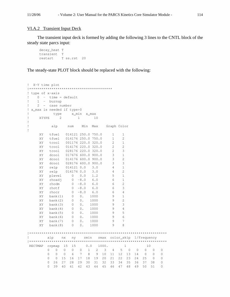
11/28/06 - Volume 2: User Manual for the PARCS Kinetics Core Simulator Module - 114
VI.A.2 Transient Input Deck
The transient input deck is formed by adding the following 3 lines to the CNTL block of thesteady state parcs input: decay_heat T transient T restart T ss.rst 20
The steady-state PLOT block should be replaced with the following:
! X-Y time plot!*****************************************! type of x-axis! 0 - time = default! 1 - burnup ! 2 - case number! x_max is needed if type>0! type x_min x_max ! XTYPE 2 1 10 !! alp num Min Max Graph Color! XY tfuel 014121 250.0 750.0 1 1 XY tfuel 014176 250.0 750.0 1 2 XY tcool 001176 220.0 320.0 2 1 XY tcool 014176 220.0 320.0 2 2 XY tcool 028176 220.0 320.0 2 3 XY dcool 017676 600.0 900.0 3 1 XY dcool 014176 600.0 900.0 3 2 XY dcool 028176 600.0 900.0 3 3 XY relp 014121 0.0 3.0 4 1 XY relp 014176 0.0 3.0 4 2 XY plevel 0 0.0 1.2 5 1 XY rhoadj 0 -8.0 6.0 6 1 XY rhodm 0 -8.0 6.0 6 2 XY rhotf 0 -8.0 6.0 6 3 XY rhocr 0 -8.0 6.0 6 4 XY bank(1) 0 0. 1000 9 1 XY bank(2) 0 0. 1000 9 2 XY bank(3) 0 0. 1000 9 3 XY bank(4) 0 0. 1000 9 4 XY bank(5) 0 0. 1000 9 5 XY bank(6) 0 0. 1000 9 6 XY bank(7) 0 0. 1000 9 7 XY bank(8) 0 0. 1000 9 8
!********************************************************************! alp nx ny zmin zmax color_skip 1/frequency!******************************************************************** RECTMAP crpmap 15 15 0.0 1000. 1 10 0 0 0 0 0 1 2 3 4 5 0 0 0 0 0 0 0 0 6 7 8 9 10 11 12 13 14 0 0 0 0 0 15 16 17 18 19 20 21 22 23 24 25 0 0 0 26 27 28 29 30 31 32 33 34 35 36 37 38 0 0 39 40 41 42 43 44 45 46 47 48 49 50 51 0

11/28/06 - Volume 2: User Manual for the PARCS Kinetics Core Simulator Module - 115
52 53 54 55 56 57 58 59 60 61 62 63 64 65 66 67 68 69 70 71 72 73 74 75 76 77 78 79 80 81 82 83 84 85 86 87 88 89 90 91 92 93 94 95 96 97 98 99 100 101 102 103 104 105 106 107 108 109 110 111 112 113 114 115 116 117 118 119 120 121 122 123 124 125 126 0 127 128 129 130 131 132 133 134 135 136 137 138 139 0 0 140 141 142 143 144 145 146 147 148 149 150 151 152 0 0 0 153 154 155 156 157 158 159 160 161 162 163 0 0 0 0 0 164 165 166 167 168 169 170 171 172 0 0 0 0 0 0 0 0 173 174 175 176 177 0 0 0 0 0
RECTMAP relp 15 15 0.5 3.0 1 10 00000 00000 00000 00000 00000 00011 00012 00013 00014 00015 00000 00000 00000 00000 00000 00000 00000 00000 00021 00022 00023 00024 00025 00026 00027 00028 00029 00000 00000 00000 00000 00000 00034 00035 00036 00037 00038 00039 00040 00041 00042 00043 00044 00000 00000 00000 00048 00049 00050 00051 00052 00053 00054 00055 00056 00057 00058 00059 00060 00000 00000 00064 00065 00066 00067 00068 00069 00070 00071 00072 00073 00074 00075 00076 00000 00080 00081 00082 00083 00084 00085 00086 00087 00088 00089 00090 00091 00092 00093 00094 00097 00098 00099 00100 00101 00102 00103 00104 00105 00106 00107 00108 00109 00110 00111 00114 00115 00116 00117 00118 00119 00120 00121 00122 00123 00124 00125 00126 00127 00128 00131 00132 00133 00134 00135 00136 00137 00138 00139 00140 00141 00142 00143 00144 00145 00148 00149 00150 00151 00152 00153 00154 00155 00156 00157 00158 00159 00160 00161 00162 00000 00166 00167 00168 00169 00170 00171 00172 00173 00174 00175 00176 00177 00178 00000 00000 00182 00183 00184 00185 00186 00187 00188 00189 00190 00191 00192 00193 00194 00000 00000 00000 00198 00199 00200 00201 00202 00203 00204 00205 00206 00207 00208 00000 00000 00000 00000 00000 00213 00214 00215 00216 00217 00218 00219 00220 00221 00000 00000 00000 00000 00000 00000 00000 00000 00227 00228 00229 00230 00231 00000 00000 00000 00000 00000! RECTMAP tcool 17 17 220.0 300.0 1 1 00000 00000 00000 00000 00000 01001 01002 01003 01004 01005 01006 01007 00000 00000 00000 00000 00000 00000 00000 00000 01008 01009 01010 01011 01012 01013 01014 01015 01016 01017 01018 00000 00000 00000 00000 00000 01019 01020 01021 01022 01023 01024 01025 01026 01027 01028 01029 01030 01031 00000 00000 00000 01032 01033 01034 01035 01036 01037 01038 01039 01040 01041 01042 01043 01044 01045 01046 00000 00000 01047 01048 01049 01050 01051 01052 01053 01054 01055 01056 01057 01058 01059 01060 01061 00000 01062 01063 01064 01065 01066 01067 01068 01069 01070 01071 01072 01073 01074 01075 01076 01077 01078 01079 01080 01081 01082 01083 01084 01085 01086 01087 01088 01089 01090 01091 01092 01093 01094 01095 01096 01097 01098 01099 01100 01101 01102 01103 01104 01105 01106 01107 01108 01109 01110 01111 01112 01113 01114 01115 01116 01117 01118 01119 01120 01121 01122 01123 01124 01125 01126 01127 01128 01129 01130 01131 01132 01133 01134 01135 01136 01137 01138 01139 01140 01141 01142 01143 01144 01145 01146 01147 01148 01149 01150 01151 01152 01153 01154 01155 01156 01157 01158 01159 01160 01161 01162 01163 01164 01165 01166 01167 01168 01169 01170 01171 01172 01173 01174 01175 01176 01177 01178 01179 01180 00000 01181 01182 01183 01184 01185 01186 01187 01188 01189 01190 01191 01192 01193 01194 01195 00000 00000 01196 01197 01198 01199 01200 01201 01202 01203 01204 01205 01206 01207 01208 01209 01210 00000 00000 00000 01211 01212 01213 01214 01215 01216 01217 01218 01219 01220 01221 01222 01223 00000 00000 00000 00000 00000 01224 01225 01226 01227 01228 01229 01230 01231 01232 01233 01234 00000 00000 00000 00000 00000 00000 00000 00000 01235 01236 01237 01238 01239 01240 01241 00000 00000 00000 00000 00000!********************************************************************! Axial Distribution Plots!********************************************************************! alp nx ny zmin zmax color_skip 1/frequency!******************************************************************** AXPLOT relp 28 4 0.0 5.0 1 1 01000 02000 03000 04000 05000 06000 07000 08000 09000 10000 11000 12000 13000 14000 15000 16000 17000 1800019000 20000 21000 22000 23000 24000 25000 26000 27000 28000 01121 02121 03121 04121 05121 06121 07121 08121 09121 10121 11121 12121 13121 14121 15121 16121 17121 1812119121 20121 21121 22121 23121 24121 25121 26121 27121 28121 01176 02176 03176 04176 05176 06176 07176 08176 09176 10176 11176 12176 13176 14176 15176 16176 17176 1817619176 20176 21176 22176 23176 24176 25176 26176 27176 28176 01050 02050 03050 04050 05050 06050 07050 08050 09050 10050 11050 12050 13050 14050 15050 16050 17050 1805019050 20050 21050 22050 23050 24050 25050 26050 27050 28050! end of plot control

11/28/06 - Volume 2: User Manual for the PARCS Kinetics Core Simulator Module - 116
VI.A.3 MAPTAB (rad.map) Input
** Method of Calculating Doppler Temperature*%DOPL LINC 0.7* AVG** Trip Unit Number for T/H Code*%TRIP 112%VOLRMAP1 vessel 99** Radial Mapping of T/H Volume Numbers to Neutronic Plane*%VOLRMAP2 0 1 2 3 4 5 6 7 8 9 10 11 12 13 14 15 16 17 1 * * * * * 20 20 20 20 20 20 20 * * * * * 2 * * * 21 21 20 14 14 14 14 14 20 19 19 * * * 3 * * 21 21 15 14 14 14 14 14 14 14 13 19 19 * * 4 * 21 21 15 15 9 8 8 8 8 8 7 13 13 19 19 * 5 * 21 15 15 15 9 8 8 8 8 8 7 13 13 13 19 * 6 21 21 15 9 9 9 3 2 2 2 1 7 7 7 13 19 19 7 21 15 15 9 9 3 3 2 2 2 1 1 7 7 13 13 19 8 21 15 15 9 9 3 3 3 2 1 1 1 7 7 13 13 19 9 21 15 15 9 9 3 3 3 2 1 1 1 7 7 13 13 19 9 22 16 16 10 10 4 4 4 5 6 6 6 12 12 18 18 2410 22 16 16 10 10 4 4 4 5 6 6 6 12 12 18 18 2411 22 16 16 10 10 4 4 5 5 5 6 6 12 12 18 18 2412 22 22 16 10 10 10 4 5 5 5 6 12 12 12 18 24 2413 * 22 16 16 16 10 11 11 11 11 11 12 18 18 18 24 *14 * 22 22 16 16 10 11 11 11 11 11 12 18 18 24 24 *15 * * 22 22 16 17 17 17 17 17 17 17 18 24 24 * *16 * * * 22 22 23 17 17 17 17 17 23 24 24 * * *17 * * * * * 23 23 23 23 23 23 23 * * * * *** Weighting Factors for %VOLRMAP2*%VOLRMAP3 0 1 2 3 4 5 6 7 8 9 10 11 12 13 14 15 16 17 1 * * * * * 1.0 1.0 1.0 1.0 1.0 1.0 1.0 * * * * * 2 * * * 1.0 1.0 1.0 1.0 1.0 1.0 1.0 1.0 1.0 1.0 1.0 * * * 3 * * 1.0 1.0 1.0 1.0 1.0 1.0 1.0 1.0 1.0 1.0 1.0 1.0 1.0 * * 4 * 1.0 1.0 1.0 1.0 1.0 1.0 1.0 1.0 1.0 1.0 1.0 1.0 1.0 1.0 1.0 * 5 * 1.0 1.0 1.0 1.0 1.0 1.0 1.0 1.0 1.0 1.0 1.0 1.0 1.0 1.0 1.0 * 6 1.0 1.0 1.0 1.0 1.0 1.0 1.0 1.0 1.0 1.0 1.0 1.0 1.0 1.0 1.0 1.0 1.0 7 1.0 1.0 1.0 1.0 1.0 1.0 1.0 1.0 1.0 1.0 1.0 1.0 1.0 1.0 1.0 1.0 1.0 8 1.0 1.0 1.0 1.0 1.0 1.0 1.0 1.0 1.0 1.0 1.0 1.0 1.0 1.0 1.0 1.0 1.0 9 0.5 0.5 0.5 0.5 0.5 0.5 0.5 0.5 0.5 0.5 0.5 0.5 0.5 0.5 0.5 0.5 0.5 9 0.5 0.5 0.5 0.5 0.5 0.5 0.5 0.5 0.5 0.5 0.5 0.5 0.5 0.5 0.5 0.5 0.510 1.0 1.0 1.0 1.0 1.0 1.0 1.0 1.0 1.0 1.0 1.0 1.0 1.0 1.0 1.0 1.0 1.011 1.0 1.0 1.0 1.0 1.0 1.0 1.0 1.0 1.0 1.0 1.0 1.0 1.0 1.0 1.0 1.0 1.012 1.0 1.0 1.0 1.0 1.0 1.0 1.0 1.0 1.0 1.0 1.0 1.0 1.0 1.0 1.0 1.0 1.013 * 1.0 1.0 1.0 1.0 1.0 1.0 1.0 1.0 1.0 1.0 1.0 1.0 1.0 1.0 1.0 *14 * 1.0 1.0 1.0 1.0 1.0 1.0 1.0 1.0 1.0 1.0 1.0 1.0 1.0 1.0 1.0 *

11/28/06 - Volume 2: User Manual for the PARCS Kinetics Core Simulator Module - 117
15 * * 1.0 1.0 1.0 1.0 1.0 1.0 1.0 1.0 1.0 1.0 1.0 1.0 1.0 * *16 * * * 1.0 1.0 1.0 1.0 1.0 1.0 1.0 1.0 1.0 1.0 1.0 * * *17 * * * * * 1.0 1.0 1.0 1.0 1.0 1.0 1.0 * * * * *
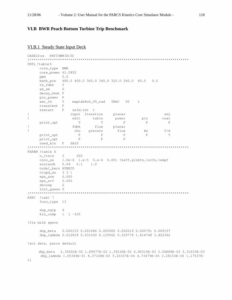
11/28/06 - Volume 2: User Manual for the PARCS Kinetics Core Simulator Module - 118
VI.B BWR Peach Bottom Turbine Trip Benchmark
VI.B.1 Steady State Input Deck
CASEID ss PBTT BWR SS 3D !****************************************************************************** CNTL !table 5 core_type BWR core_power 61.5852 ppm 0.0 bank_pos 480.0 400.0 360.0 340.0 320.0 260.0 40.0 0.0 th_fdbk T xe_sm 0 decay_heat F pin_power F ext_th T maptab8ch_05_rad TRAC 50 1 transient F restart F ss3d.rst 1! input iteration planar adj! edit table power pin reac print_opt T T F F F! fdbk flux planar! rho precurs flux Xe T/H print_opt F F F F T print_opt F F F oned_kin F SA1D!******************************************************************************PARAM !table 6 n_iters 5 500 conv_ss 1.0e-6 1.e-5 5.e-4 0.001 !keff,globfs,locfs,tempf wielandt 0.04 0.1 1.0 nodal_kern HYBRID nlupd_ss 3 3 1 eps_anm 0.005 eps_erf 0.005 decusp 2 init_guess 0!******************************************************************************XSEC !tabl 7 func_type 13 dnp_ngrp 6 kin_comp 1 1 -435 !fix mslb specs dnp_beta 0.000153 0.001086 0.000965 0.002019 0.000791 0.000197 dnp_lambda 0.012818 0.031430 0.125062 0.329776 1.414748 3.822362 !anl data, parcs default dhp_beta 2.35402E-02 1.89077E-02 1.39236E-02 6.90315E-03 3.56888E-03 3.31633E-03 dhp_lambda 1.05345E-01 8.37149E-03 5.20337E-04 4.73479E-05 3.28153E-06 1.17537E-11
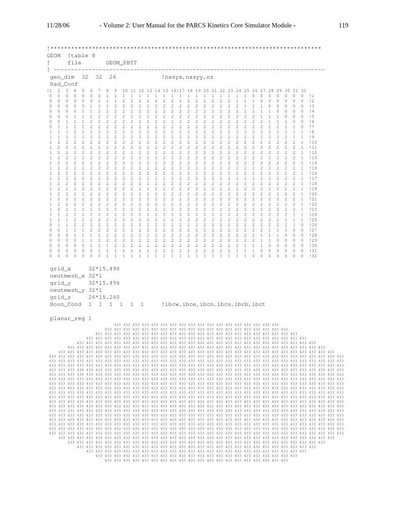
11/28/06 - Volume 2: User Manual for the PARCS Kinetics Core Simulator Module - 119
!******************************************************************************GEOM !table 8! file GEOM_PBTT! ------------------------------------------------------------------------------ geo_dim 32 32 26 !nasyx,nasyy,nz Rad_Conf!1 2 3 4 5 6 7 8 9 10 11 12 13 14 15 16|17 18 19 20 21 22 23 24 25 26 27 28 29 30 31 32 0 0 0 0 0 0 0 1 1 1 1 1 1 1 1 1 1 1 1 1 1 1 1 1 1 0 0 0 0 0 0 0 !1 0 0 0 0 0 0 1 1 1 2 2 2 2 2 2 2 2 2 2 2 2 2 2 1 1 1 0 0 0 0 0 0 !2 0 0 0 0 0 1 1 1 2 2 2 2 2 2 2 2 2 2 2 2 2 2 2 2 1 1 1 0 0 0 0 0 !3 0 0 0 0 1 1 2 2 2 2 2 2 2 2 2 2 2 2 2 2 2 2 2 2 2 2 1 1 0 0 0 0 !4 0 0 0 1 1 1 2 2 2 2 2 2 2 2 2 2 2 2 2 2 2 2 2 2 2 2 1 1 1 0 0 0 !5 0 0 1 1 1 2 2 2 2 2 2 2 2 2 2 2 2 2 2 2 2 2 2 2 2 2 2 1 1 1 0 0 !6 0 1 1 2 2 2 2 2 2 2 2 2 2 2 2 2 2 2 2 2 2 2 2 2 2 2 2 2 2 1 1 0 !7 1 1 1 2 2 2 2 2 2 2 2 2 2 2 2 2 2 2 2 2 2 2 2 2 2 2 2 2 2 1 1 1 !8 1 1 2 2 2 2 2 2 2 2 2 2 2 2 2 2 2 2 2 2 2 2 2 2 2 2 2 2 2 2 1 1 !9 1 2 2 2 2 2 2 2 2 2 2 2 2 2 2 2 2 2 2 2 2 2 2 2 2 2 2 2 2 2 2 1 !10 1 2 2 2 2 2 2 2 2 2 2 2 2 2 2 2 2 2 2 2 2 2 2 2 2 2 2 2 2 2 2 1 !11 1 2 2 2 2 2 2 2 2 2 2 2 2 2 2 2 2 2 2 2 2 2 2 2 2 2 2 2 2 2 2 1 !12 1 2 2 2 2 2 2 2 2 2 2 2 2 2 2 2 2 2 2 2 2 2 2 2 2 2 2 2 2 2 2 1 !13 1 2 2 2 2 2 2 2 2 2 2 2 2 2 2 2 2 2 2 2 2 2 2 2 2 2 2 2 2 2 2 1 !14 1 2 2 2 2 2 2 2 2 2 2 2 2 2 2 2 2 2 2 2 2 2 2 2 2 2 2 2 2 2 2 1 !15 1 2 2 2 2 2 2 2 2 2 2 2 2 2 2 2 2 2 2 2 2 2 2 2 2 2 2 2 2 2 2 1 !16 1 2 2 2 2 2 2 2 2 2 2 2 2 2 2 2 2 2 2 2 2 2 2 2 2 2 2 2 2 2 2 1 !17 1 2 2 2 2 2 2 2 2 2 2 2 2 2 2 2 2 2 2 2 2 2 2 2 2 2 2 2 2 2 2 1 !18 1 2 2 2 2 2 2 2 2 2 2 2 2 2 2 2 2 2 2 2 2 2 2 2 2 2 2 2 2 2 2 1 !19 1 2 2 2 2 2 2 2 2 2 2 2 2 2 2 2 2 2 2 2 2 2 2 2 2 2 2 2 2 2 2 1 !20 1 2 2 2 2 2 2 2 2 2 2 2 2 2 2 2 2 2 2 2 2 2 2 2 2 2 2 2 2 2 2 1 !21 1 2 2 2 2 2 2 2 2 2 2 2 2 2 2 2 2 2 2 2 2 2 2 2 2 2 2 2 2 2 2 1 !22 1 2 2 2 2 2 2 2 2 2 2 2 2 2 2 2 2 2 2 2 2 2 2 2 2 2 2 2 2 2 2 1 !23 1 1 2 2 2 2 2 2 2 2 2 2 2 2 2 2 2 2 2 2 2 2 2 2 2 2 2 2 2 2 1 1 !24 1 1 1 2 2 2 2 2 2 2 2 2 2 2 2 2 2 2 2 2 2 2 2 2 2 2 2 2 2 1 1 1 !25 0 1 1 2 2 2 2 2 2 2 2 2 2 2 2 2 2 2 2 2 2 2 2 2 2 2 2 2 2 1 1 0 !26 0 0 1 1 1 2 2 2 2 2 2 2 2 2 2 2 2 2 2 2 2 2 2 2 2 2 2 1 1 1 0 0 !27 0 0 0 1 1 1 2 2 2 2 2 2 2 2 2 2 2 2 2 2 2 2 2 2 2 2 1 1 1 0 0 0 !28 0 0 0 0 1 1 2 2 2 2 2 2 2 2 2 2 2 2 2 2 2 2 2 2 2 2 1 1 0 0 0 0 !29 0 0 0 0 0 1 1 1 2 2 2 2 2 2 2 2 2 2 2 2 2 2 2 2 1 1 1 0 0 0 0 0 !30 0 0 0 0 0 0 1 1 1 2 2 2 2 2 2 2 2 2 2 2 2 2 2 1 1 1 0 0 0 0 0 0 !31 0 0 0 0 0 0 0 1 1 1 1 1 1 1 1 1 1 1 1 1 1 1 1 1 1 0 0 0 0 0 0 0 !32 grid_x 32*15.494 neutmesh_x 32*1 grid_y 32*15.494 neutmesh_y 32*1 grid_z 26*15.240 Boun_Cond 1 1 1 1 1 1 !ibcw,ibce,ibcn,ibcs,ibcb,ibct planar_reg 1 433 433 433 433 433 433 433 433 433 433 433 433 433 433 433 433 433 433 433 433 433 433 433 433 433 433 433 433 433 433 433 433 433 433 433 433 433 433 433 433 433 433 433 433 433 433 433 433 433 433 433 433 433 433 433 433 433 433 433 433 433 433 433 433 433 433 433 433 433 433 433 433 433 433 433 433 433 433 433 433 433 433 433 433 433 433 433 433 433 433 433 433 433 433 433 433 433 433 433 433 433 433 433 433 433 433 433 433 433 433 433 433 433 433 433 433 433 433 433 433 433 433 433 433 433 433 433 433 433 433 433 433 433 433 433 433 433 433 433 433 433 433 433 433 433 433 433 433 433 433 433 433 433 433 433 433 433 433 433 433 433 433 433 433 433 433 433 433 433 433 433 433 433 433 433 433 433 433 433 433 433 433 433 433 433 433 433 433 433 433 433 433 433 433 433 433 433 433 433 433 433 433 433 433 433 433 433 433 433 433 433 433 433 433 433 433 433 433 433 433 433 433 433 433 433 433 433 433 433 433 433 433 433 433 433 433 433 433 433 433 433 433 433 433 433 433 433 433 433 433 433 433 433 433 433 433 433 433 433 433 433 433 433 433 433 433 433 433 433 433 433 433 433 433 433 433 433 433 433 433 433 433 433 433 433 433 433 433 433 433 433 433 433 433 433 433 433 433 433 433 433 433 433 433 433 433 433 433 433 433 433 433 433 433 433 433 433 433 433 433 433 433 433 433 433 433 433 433 433 433 433 433 433 433 433 433 433 433 433 433 433 433 433 433 433 433 433 433 433 433 433 433 433 433 433 433 433 433 433 433 433 433 433 433 433 433 433 433 433 433 433 433 433 433 433 433 433 433 433 433 433 433 433 433 433 433 433 433 433 433 433 433 433 433 433 433 433 433 433 433 433 433 433 433 433 433 433 433 433 433 433 433 433 433 433 433 433 433 433 433 433 433 433 433 433 433 433 433 433 433 433 433 433 433 433 433 433 433 433 433 433 433 433 433 433 433 433 433 433 433 433 433 433 433 433 433 433 433 433 433 433 433 433 433 433 433 433 433 433 433 433 433 433 433 433 433 433 433 433 433 433 433 433 433 433 433 433 433 433 433 433 433 433 433 433 433 433 433 433 433 433 433 433 433 433 433 433 433 433 433 433 433 433 433 433 433 433 433 433 433 433 433 433 433 433 433 433 433 433 433 433 433 433 433 433 433 433 433 433 433 433 433 433 433 433 433 433 433 433 433 433 433 433 433 433 433 433 433 433 433 433 433 433 433 433 433 433 433 433 433 433 433 433 433 433 433 433 433 433 433 433 433 433 433 433 433 433 433 433 433 433 433 433 433 433 433 433 433 433 433 433 433 433 433 433 433 433 433 433 433 433 433 433 433 433 433 433 433 433 433 433 433 433 433 433 433 433 433 433 433 433 433 433 433 433 433 433 433 433 433 433 433 433 433 433 433 433 433 433 433 433 433 433 433 433 433 433 433 433 433 433 433 433 433 433 433 433 433 433 433 433 433 433 433 433 433 433 433 433 433 433 433 433 433 433 433 433 433 433 433 433 433 433 433 433 433 433 433 433 433 433 433 433 433 433 433 433 433 433 433 433 433 433 433 433 433 433 433 433 433 433 433 433 433 433 433 433 433 433 433 433 433 433 433 433 433 433 433 433 433 433 433 433 433 433 433 433 433 433 433 433 433 433 433 433 433 433 433 433 433 433 433 433 433 433 433 433 433 433 433 433 433 433 433 433 433 433 433 433 433 433 433 433 433 433 433 433 433 433 433 433 433 433 433 433 433 433 433 433 433 433 433 433 433 433 433 433 433 433 433 433 433 433 433 433 433 433 433 433 433 433 433 433 433 433 433 433 433 433 433 433 433 433 433 433 433 433 433 433 433 433 433 433 433 433 433 433 433 433 433 433 433 433 433 433 433 433 433 433 433 433 433 433 433 433 433 433 433 433 433 433 433 433 433 433 433 433 433 433 433 433 433 433 433 433 433 433 433 433 433 433 433 433 433
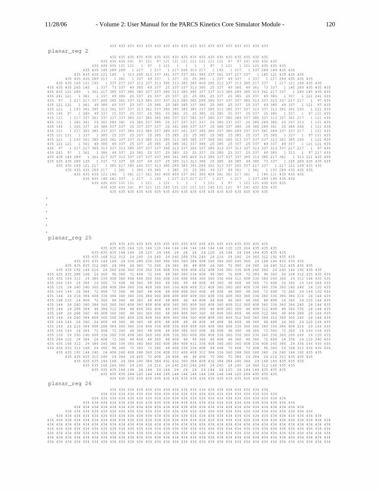
11/28/06 - Volume 2: User Manual for the PARCS Kinetics Core Simulator Module - 120
433 433 433 433 433 433 433 433 433 433 433 433 433 433 433 433 433 433
planar_reg 2 435 435 435 435 435 435 435 435 435 435 435 435 435 435 435 435 435 435 435 435 435 241 97 121 97 121 121 121 121 121 121 121 97 97 241 435 435 435 435 435 435 121 121 1 97 1 121 1 1 1 1 97 1 121 1 121 121 435 435 435 435 435 145 289 289 1 217 1 217 1 217 265 313 217 1 193 1 217 1 337 289 169 435 435 435 435 435 121 145 1 313 265 313 337 361 337 337 361 385 337 361 337 217 337 1 145 121 435 435 435 435 435 435 289 217 1 361 1 337 49 337 1 337 25 25 385 1 337 49 337 1 337 1 217 289 435 435 435 435 435 169 121 193 1 337 217 337 313 337 313 385 313 385 385 409 385 313 337 313 385 217 337 1 217 121 169 435 435 435 435 435 265 145 1 337 73 337 49 385 49 337 25 337 337 313 385 25 337 49 385 49 361 73 337 1 145 289 435 435 435 435 435 121 289 1 361 217 385 337 385 385 337 337 385 313 385 385 337 337 313 385 289 385 313 361 217 337 1 289 145 435 435 435 241 121 1 361 1 337 49 385 25 337 25 337 25 337 25 25 385 25 337 25 385 25 337 49 385 1 337 1 121 241 435 435 97 1 217 217 337 265 385 361 337 313 385 337 337 313 385 385 289 385 337 337 337 385 313 337 313 337 217 217 1 97 435 435 121 121 1 361 49 385 49 337 25 337 25 385 25 385 385 337 385 25 385 25 337 25 337 49 385 49 337 1 121 97 435 435 121 1 193 361 385 313 361 337 337 313 361 337 385 385 385 385 337 385 313 385 337 337 313 337 313 361 361 193 1 121 435 435 145 97 1 385 49 337 25 337 25 337 25 385 25 385 25 25 385 25 385 25 337 25 337 25 385 1 337 1 97 121 435 435 121 1 217 337 361 337 337 337 385 337 385 385 385 337 337 385 337 385 337 385 289 337 385 337 313 337 361 217 1 121 435 435 121 1 265 361 25 361 289 361 25 385 337 385 25 337 337 337 337 25 385 337 337 25 385 289 385 25 337 313 1 121 435 435 145 1 265 337 25 385 337 337 25 337 337 337 25 361 385 337 337 25 385 337 385 25 385 289 361 25 385 265 1 121 435 435 121 1 217 361 385 337 337 337 385 313 385 337 385 337 361 337 385 385 337 385 289 337 337 361 289 337 337 217 1 121 435 435 121 121 1 337 1 385 25 337 25 337 25 385 25 385 25 25 385 25 385 25 385 25 337 25 385 1 337 1 97 121 435 435 121 1 193 361 385 265 361 337 337 313 385 313 385 313 385 385 337 385 361 385 313 337 337 337 313 361 385 193 1 121 435 435 121 121 1 361 49 385 49 337 25 337 25 385 25 385 361 337 385 25 385 25 337 25 337 49 337 49 337 1 121 121 435 435 97 1 217 217 385 313 337 313 385 337 337 337 385 313 337 385 337 385 313 337 313 337 313 337 313 337 217 217 1 97 435 435 241 97 1 361 1 385 49 337 25 385 25 337 25 385 25 25 337 25 385 25 337 25 337 49 385 1 313 1 97 217 435 435 435 145 289 1 361 217 337 313 337 337 337 337 385 361 385 409 313 385 337 337 337 385 313 385 217 361 1 313 121 435 435 435 435 435 289 145 1 337 73 337 49 337 49 337 25 385 313 313 385 25 385 49 385 49 385 73 337 1 145 289 435 435 435 435 435 169 121 217 1 385 217 385 265 337 313 385 289 385 385 289 361 313 337 265 337 217 337 1 217 121 169 435 435 435 435 435 289 217 1 361 1 385 49 385 1 385 25 25 385 49 337 49 361 1 361 1 193 289 435 435 435 435 435 435 121 145 1 361 217 361 361 409 409 337 361 385 409 361 361 217 361 1 145 121 435 435 435 435 435 145 241 337 1 217 1 193 1 217 217 217 217 1 217 1 217 1 337 289 145 435 435 435 435 435 121 121 1 121 1 121 1 1 1 1 121 1 97 1 121 121 435 435 435 435 435 435 241 97 121 121 145 121 121 121 121 145 121 121 97 241 435 435 435 435 435 435 435 435 435 435 435 435 435 435 435 435 435 435 435 435 435
.
.
.
.
.
. planar_reg 25 435 435 435 435 435 435 435 435 435 435 435 435 435 435 435 435 435 435 435 435 435 264 120 144 120 144 144 144 144 144 144 144 120 120 264 435 435 435 435 435 435 144 144 24 120 24 144 24 24 24 24 120 24 144 24 144 144 435 435 435 435 435 168 312 312 24 240 24 240 24 240 288 336 240 24 216 24 240 24 360 312 192 435 435 435 435 435 144 168 24 336 288 336 360 384 360 360 384 408 360 384 360 240 360 24 168 144 435 435 435 435 435 435 312 240 24 384 24 360 72 360 24 360 48 48 408 24 360 72 360 24 360 24 240 312 435 435 435 435 435 192 144 216 24 360 240 360 336 360 336 408 336 408 408 432 408 336 360 336 408 240 360 24 240 144 192 435 435 435 435 435 288 168 24 360 96 360 72 408 72 360 48 360 360 336 408 48 360 72 408 72 384 96 360 24 168 312 435 435 435 435 435 144 312 24 384 240 408 360 408 408 360 360 408 336 408 408 360 360 336 408 312 408 336 384 240 360 24 312 168 435 435 435 264 144 24 384 24 360 72 408 48 360 48 360 48 360 48 48 408 48 360 48 408 48 360 72 408 24 360 24 144 264 435 435 120 24 240 240 360 288 408 384 360 336 408 360 360 336 408 408 312 408 360 360 360 408 336 360 336 360 240 240 24 120 435 435 144 144 24 384 72 408 72 360 48 360 48 408 48 408 408 360 408 48 408 48 360 48 360 72 408 72 360 24 144 120 435 435 144 24 216 384 408 336 384 360 360 336 384 360 408 408 408 408 360 408 336 408 360 360 336 360 336 384 384 216 24 144 435 435 168 120 24 408 72 360 48 360 48 360 48 408 48 408 48 48 408 48 408 48 360 48 360 48 408 24 360 24 120 144 435 435 144 24 240 360 384 360 360 360 408 360 408 408 408 360 360 408 360 408 360 408 312 360 408 360 336 360 384 240 24 144 435 435 144 24 288 384 48 384 312 384 48 408 360 408 48 360 360 360 360 48 408 360 360 48 408 312 408 48 360 336 24 144 435 435 168 24 288 360 48 408 360 360 48 360 360 360 48 384 408 360 360 48 408 360 408 48 408 312 384 48 408 288 24 144 435 435 144 24 240 384 408 360 360 360 408 336 408 360 408 360 384 360 408 408 360 408 312 360 360 384 312 360 360 240 24 144 435 435 144 144 24 360 24 408 48 360 48 360 48 408 48 408 48 48 408 48 408 48 408 48 360 48 408 24 360 24 120 144 435 435 144 24 216 384 408 288 384 360 360 336 408 336 408 336 408 408 360 408 384 408 336 360 360 360 336 384 408 216 24 144 435 435 144 144 24 384 72 408 72 360 48 360 48 408 48 408 384 360 408 48 408 48 360 48 360 72 360 72 360 24 144 144 435 435 120 24 240 240 408 336 360 336 408 360 360 360 408 336 360 408 360 408 336 360 336 360 336 360 336 360 240 240 24 120 435 435 264 120 24 384 24 408 72 360 48 408 48 360 48 408 48 48 360 48 408 48 360 48 360 72 408 24 336 24 120 240 435 435 435 168 312 24 384 240 360 336 360 360 360 360 408 384 408 432 336 408 360 360 360 408 336 408 240 384 24 336 144 435 435 435 435 435 312 168 24 360 96 360 72 360 72 360 48 408 336 336 408 48 408 72 408 72 408 96 360 24 168 312 435 435 435 435 435 192 144 240 24 408 240 408 288 360 336 408 312 408 408 312 384 336 360 288 360 240 360 24 240 144 192 435 435 435 435 435 312 240 24 384 24 408 72 408 24 408 48 48 408 72 360 72 384 24 384 24 216 312 435 435 435 435 435 435 144 168 24 384 240 384 384 432 432 360 384 408 432 384 384 240 384 24 168 144 435 435 435 435 435 168 264 360 24 240 24 216 24 240 240 240 240 24 240 24 240 24 360 312 168 435 435 435 435 435 144 144 24 144 24 144 24 24 24 24 144 24 120 24 144 144 435 435 435 435 435 435 264 120 144 144 168 144 144 144 144 168 144 144 120 264 435 435 435 435 435 435 435 435 435 435 435 435 435 435 435 435 435 435 435 435 435
planar_reg 26 434 434 434 434 434 434 434 434 434 434 434 434 434 434 434 434 434 434 434 434 434 434 434 434 434 434 434 434 434 434 434 434 434 434 434 434 434 434 434 434 434 434 434 434 434 434 434 434 434 434 434 434 434 434 434 434 434 434 434 434 434 434 434 434 434 434 434 434 434 434 434 434 434 434 434 434 434 434 434 434 434 434 434 434 434 434 434 434 434 434 434 434 434 434 434 434 434 434 434 434 434 434 434 434 434 434 434 434 434 434 434 434 434 434 434 434 434 434 434 434 434 434 434 434 434 434 434 434 434 434 434 434 434 434 434 434 434 434 434 434 434 434 434 434 434 434 434 434 434 434 434 434 434 434 434 434 434 434 434 434 434 434 434 434 434 434 434 434 434 434 434 434 434 434 434 434 434 434 434 434 434 434 434 434 434 434 434 434 434 434 434 434 434 434 434 434 434 434 434 434 434 434 434 434 434 434 434 434 434 434 434 434 434 434 434 434 434 434 434 434 434 434 434 434 434 434 434 434 434 434 434 434 434 434 434 434 434 434 434 434 434 434 434 434 434 434 434 434 434 434 434 434 434 434 434 434 434 434 434 434 434 434 434 434 434 434 434 434 434 434 434 434 434 434 434 434 434 434 434 434 434 434 434 434 434 434 434 434 434 434 434 434 434 434 434 434 434 434 434 434 434 434 434 434 434 434 434 434 434 434 434 434 434 434 434 434 434 434 434 434 434 434 434 434 434 434 434 434 434 434 434 434 434 434 434 434 434 434 434 434 434 434 434 434 434 434 434 434 434 434 434 434 434 434 434 434 434 434 434 434
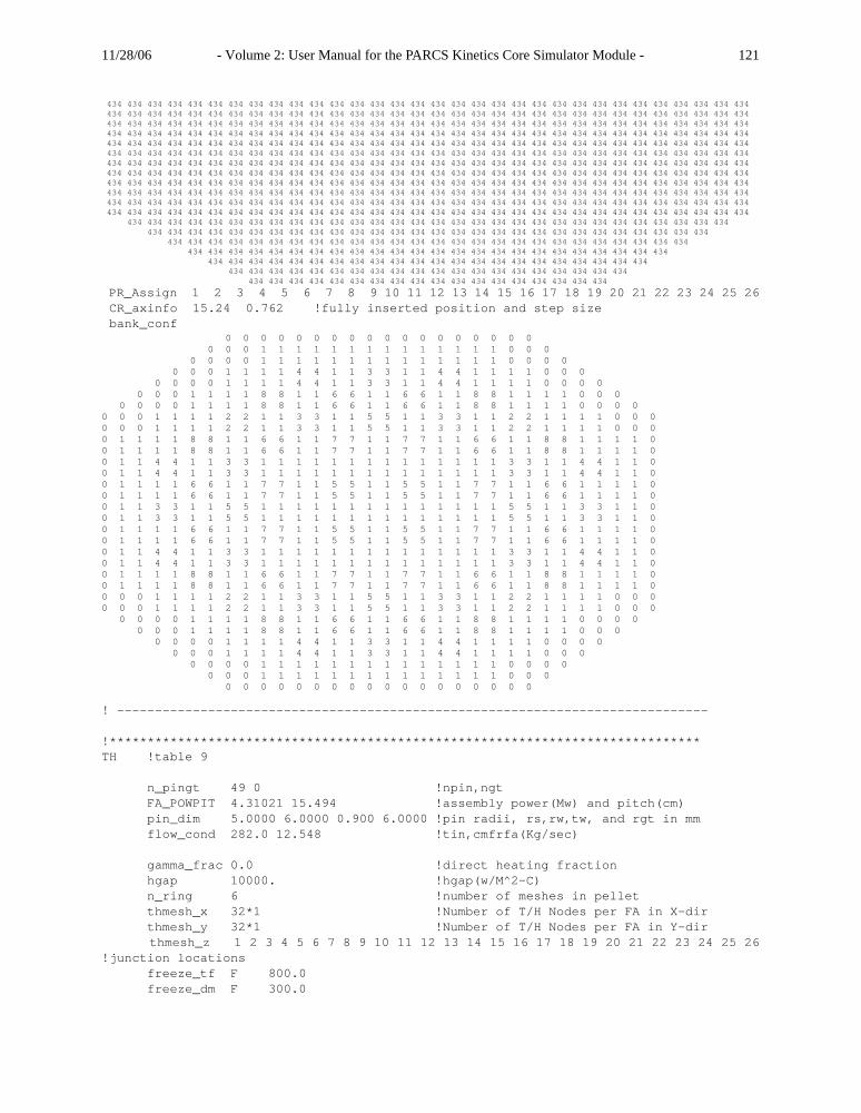
11/28/06 - Volume 2: User Manual for the PARCS Kinetics Core Simulator Module - 121
434 434 434 434 434 434 434 434 434 434 434 434 434 434 434 434 434 434 434 434 434 434 434 434 434 434 434 434 434 434 434 434 434 434 434 434 434 434 434 434 434 434 434 434 434 434 434 434 434 434 434 434 434 434 434 434 434 434 434 434 434 434 434 434 434 434 434 434 434 434 434 434 434 434 434 434 434 434 434 434 434 434 434 434 434 434 434 434 434 434 434 434 434 434 434 434 434 434 434 434 434 434 434 434 434 434 434 434 434 434 434 434 434 434 434 434 434 434 434 434 434 434 434 434 434 434 434 434 434 434 434 434 434 434 434 434 434 434 434 434 434 434 434 434 434 434 434 434 434 434 434 434 434 434 434 434 434 434 434 434 434 434 434 434 434 434 434 434 434 434 434 434 434 434 434 434 434 434 434 434 434 434 434 434 434 434 434 434 434 434 434 434 434 434 434 434 434 434 434 434 434 434 434 434 434 434 434 434 434 434 434 434 434 434 434 434 434 434 434 434 434 434 434 434 434 434 434 434 434 434 434 434 434 434 434 434 434 434 434 434 434 434 434 434 434 434 434 434 434 434 434 434 434 434 434 434 434 434 434 434 434 434 434 434 434 434 434 434 434 434 434 434 434 434 434 434 434 434 434 434 434 434 434 434 434 434 434 434 434 434 434 434 434 434 434 434 434 434 434 434 434 434 434 434 434 434 434 434 434 434 434 434 434 434 434 434 434 434 434 434 434 434 434 434 434 434 434 434 434 434 434 434 434 434 434 434 434 434 434 434 434 434 434 434 434 434 434 434 434 434 434 434 434 434 434 434 434 434 434 434 434 434 434 434 434 434 434 434 434 434 434 434 434 434 434 434 434 434 434 434 434 434 434 434 434 434 434 434 434 434 434 434 434 434 434 434 434 434 434 434 434 434 434 434 434 434 434 434 434 434 434 434 434 434 434 434 434 434 434 434 434 434 434 434 434 434 434 434 434 434 434 434 434 434 434 434 434 434 434 434 434 434 434 434 434 434 434 434 434 434 434 434 434 434 434 434 434 434 434 434 434 434 434 434 434 434 434 434 434 434 434 434 434 434 434 434 434 434 434 434 434 434 434 434 434 434 434 434 434 434 434 434 434 434 434 434 434 434 434 434 434 434 434 434 434 434 434 434 434 434 434 434 434 434 434 434 434 434 434 434 434 434 434 434 434 434 434 434 434 434 434 434 434 434 434 434 434 434 434 434 434 434 434 434 434 434 434 434 434 434 434 434
PR_Assign 1 2 3 4 5 6 7 8 9 10 11 12 13 14 15 16 17 18 19 20 21 22 23 24 25 26 CR_axinfo 15.24 0.762 !fully inserted position and step size bank_conf 0 0 0 0 0 0 0 0 0 0 0 0 0 0 0 0 0 0 0 0 0 1 1 1 1 1 1 1 1 1 1 1 1 1 1 0 0 0 0 0 0 0 1 1 1 1 1 1 1 1 1 1 1 1 1 1 0 0 0 0 0 0 0 1 1 1 1 4 4 1 1 3 3 1 1 4 4 1 1 1 1 0 0 0 0 0 0 0 1 1 1 1 4 4 1 1 3 3 1 1 4 4 1 1 1 1 0 0 0 0 0 0 0 1 1 1 1 8 8 1 1 6 6 1 1 6 6 1 1 8 8 1 1 1 1 0 0 0 0 0 0 0 1 1 1 1 8 8 1 1 6 6 1 1 6 6 1 1 8 8 1 1 1 1 0 0 0 00 0 0 1 1 1 1 2 2 1 1 3 3 1 1 5 5 1 1 3 3 1 1 2 2 1 1 1 1 0 0 00 0 0 1 1 1 1 2 2 1 1 3 3 1 1 5 5 1 1 3 3 1 1 2 2 1 1 1 1 0 0 00 1 1 1 1 8 8 1 1 6 6 1 1 7 7 1 1 7 7 1 1 6 6 1 1 8 8 1 1 1 1 00 1 1 1 1 8 8 1 1 6 6 1 1 7 7 1 1 7 7 1 1 6 6 1 1 8 8 1 1 1 1 00 1 1 4 4 1 1 3 3 1 1 1 1 1 1 1 1 1 1 1 1 1 1 3 3 1 1 4 4 1 1 00 1 1 4 4 1 1 3 3 1 1 1 1 1 1 1 1 1 1 1 1 1 1 3 3 1 1 4 4 1 1 00 1 1 1 1 6 6 1 1 7 7 1 1 5 5 1 1 5 5 1 1 7 7 1 1 6 6 1 1 1 1 00 1 1 1 1 6 6 1 1 7 7 1 1 5 5 1 1 5 5 1 1 7 7 1 1 6 6 1 1 1 1 00 1 1 3 3 1 1 5 5 1 1 1 1 1 1 1 1 1 1 1 1 1 1 5 5 1 1 3 3 1 1 00 1 1 3 3 1 1 5 5 1 1 1 1 1 1 1 1 1 1 1 1 1 1 5 5 1 1 3 3 1 1 00 1 1 1 1 6 6 1 1 7 7 1 1 5 5 1 1 5 5 1 1 7 7 1 1 6 6 1 1 1 1 00 1 1 1 1 6 6 1 1 7 7 1 1 5 5 1 1 5 5 1 1 7 7 1 1 6 6 1 1 1 1 00 1 1 4 4 1 1 3 3 1 1 1 1 1 1 1 1 1 1 1 1 1 1 3 3 1 1 4 4 1 1 00 1 1 4 4 1 1 3 3 1 1 1 1 1 1 1 1 1 1 1 1 1 1 3 3 1 1 4 4 1 1 00 1 1 1 1 8 8 1 1 6 6 1 1 7 7 1 1 7 7 1 1 6 6 1 1 8 8 1 1 1 1 00 1 1 1 1 8 8 1 1 6 6 1 1 7 7 1 1 7 7 1 1 6 6 1 1 8 8 1 1 1 1 00 0 0 1 1 1 1 2 2 1 1 3 3 1 1 5 5 1 1 3 3 1 1 2 2 1 1 1 1 0 0 00 0 0 1 1 1 1 2 2 1 1 3 3 1 1 5 5 1 1 3 3 1 1 2 2 1 1 1 1 0 0 0 0 0 0 0 1 1 1 1 8 8 1 1 6 6 1 1 6 6 1 1 8 8 1 1 1 1 0 0 0 0 0 0 0 1 1 1 1 8 8 1 1 6 6 1 1 6 6 1 1 8 8 1 1 1 1 0 0 0 0 0 0 0 1 1 1 1 4 4 1 1 3 3 1 1 4 4 1 1 1 1 0 0 0 0 0 0 0 1 1 1 1 4 4 1 1 3 3 1 1 4 4 1 1 1 1 0 0 0 0 0 0 0 1 1 1 1 1 1 1 1 1 1 1 1 1 1 0 0 0 0 0 0 0 1 1 1 1 1 1 1 1 1 1 1 1 1 1 0 0 0 0 0 0 0 0 0 0 0 0 0 0 0 0 0 0 0 0 0 ! ------------------------------------------------------------------------------ !******************************************************************************TH !table 9 n_pingt 49 0 !npin,ngt FA_POWPIT 4.31021 15.494 !assembly power(Mw) and pitch(cm) pin_dim 5.0000 6.0000 0.900 6.0000 !pin radii, rs,rw,tw, and rgt in mm flow_cond 282.0 12.548 !tin,cmfrfa(Kg/sec) gamma_frac 0.0 !direct heating fraction hgap 10000. !hgap(w/M^2-C) n_ring 6 !number of meshes in pellet thmesh_x 32*1 !Number of T/H Nodes per FA in X-dir thmesh_y 32*1 !Number of T/H Nodes per FA in Y-dir thmesh_z 1 2 3 4 5 6 7 8 9 10 11 12 13 14 15 16 17 18 19 20 21 22 23 24 25 26!junction locations freeze_tf F 800.0 freeze_dm F 300.0

11/28/06 - Volume 2: User Manual for the PARCS Kinetics Core Simulator Module - 122
write_fbv T ss3d.fbv read_dopl F ss3d.fbv read_tmdm F ss3d.fbv!******************************************************************************!PFF table 10, power form function!******************************************************************************PLOT! file sscoupl.plc! ------------------------------------------------------------------------------! X-Y time plot!*****************************************! type of x-axis! 0 - time = default! 1 - sstime! 2 - case number! x_max is needed if type>0! type x_min x_max XTYPE 1 0 80!! alp num Min Max Graph Color! XY tfuel 013460 250.0 750.0 1 1 XY tfuel 013472 250.0 750.0 1 2 XY tcool 001472 280.0 300.0 2 1 XY tcool 013472 280.0 300.0 2 2 XY tcool 026472 280.0 300.0 2 3 XY relp 013460 0.0 1.9 4 1 XY relp 013472 0.0 1.9 4 2 XY keff 0 1.000 1.010 5 1 XY vcool 001472 0.0 1.0 6 1 XY vcool 013472 0.0 1.0 6 2 XY vcool 026472 0.0 1.0 6 3
!********************************************************************! alp nx ny zmin zmax color_skip 1/frequency!******************************************************************** RECTMAP lp2d 30 30 0.0 500. 1 10 0 0 0 0 0 0 0 0 1 2 3 4 5 6 7 8 9 10 11 12 13 14 0 0 0 0 0 0 0 0 0 0 0 0 0 0 0 15 16 17 18 19 20 21 22 23 24 25 26 27 28 29 30 0 0 0 0 0 0 0 0 0 0 0 0 31 32 33 34 35 36 37 38 39 40 41 42 43 44 45 46 47 48 49 50 0 0 0 0 0 0 0 0 0 0 51 52 53 54 55 56 57 58 59 60 61 62 63 64 65 66 67 68 69 70 0 0 0 0 0 0 0 0 0 71 72 73 74 75 76 77 78 79 80 81 82 83 84 85 86 87 88 89 90 91 92 0 0 0 0 0 0 93 94 95 96 97 98 99 100 101 102 103 104 105 106 107 108 109 110 111 112 113 114 115 116 117 118 0 0 0 0 119 120 121 122 123 124 125 126 127 128 129 130 131 132 133 134 135 136 137 138 139 140 141 142 143 144 0 0 0 145 146 147 148 149 150 151 152 153 154 155 156 157 158 159 160 161 162 163 164 165 166 167 168 169 170 171 172 0 173 174 175 176 177 178 179 180 181 182 183 184 185 186 187 188 189 190 191 192 193 194 195 196 197 198 199 200 201 202 203 204 205 206 207 208 209 210 211 212 213 214 215 216 217 218 219 220 221 222 223 224 225 226 227 228 229 230 231 232 233 234 235 236 237 238 239 240 241 242 243 244 245 246 247 248 249 250 251 252 253 254 255 256 257 258 259 260 261 262 263 264 265 266 267 268 269 270 271 272 273 274 275 276 277 278 279 280 281 282 283 284 285 286 287 288 289 290 291 292 293 294 295 296 297 298 299 300 301 302 303 304 305 306 307 308 309 310 311 312 313 314 315 316 317 318 319 320 321 322 323 324 325 326 327 328 329 330 331 332 333 334 335 336 337 338 339 340 341 342 343 344 345 346 347 348 349 350 351 352 353 354 355 356 357 358 359 360 361 362 363 364 365 366 367 368 369 370 371 372 373 374 375 376 377 378 379 380 381 382 383 384 385 386 387 388 389 390 391 392 393 394 395 396 397 398 399 400 401 402 403 404 405 406 407 408 409 410 411 412 413 414 415 416 417 418 419 420 421 422 423 424 425 426 427 428 429 430 431 432 433 434 435 436 437 438 439 440 441 442 443 444 445 446 447 448 449 450 451 452 453 454 455 456 457 458 459 460 461 462 463 464 465 466 467 468 469 470 471 472 473 474 475 476 477 478 479 480 481 482 483 484 485 486 487 488 489 490 491 492 493 494 495 496 497 498 499 500 501 502 503 504 505 506 507 508 509 510 511 512 513 514 515 516 517 518 519 520 521 522 523 524 525 526 527 528 529 530 531 532 533 534 535 536 537 538 539 540 541 542 543 544 545 546 547 548 549 550 551 552 553 554 555 556 557 558 559 560 561 562 563 564 565 566 567 568 569 570 571 572 573 574 575 576 577 578 579 580 581 582 583 584 585 586 587 588 589 590 591 592 0 593 594 595 596 597 598 599 600 601 602 603 604 605 606 607 608 609 610 611 612 613 614 615 616 617 618 619 620 0 0 0 621 622 623 624 625 626 627 628 629 630 631 632 633 634 635 636 637 638 639 640 641 642 643 644 645 646 0 0 0 0 647 648 649 650 651 652 653 654 655 656 657 658 659 660 661 662 663 664 665 666 667 668 669 670 671 672 0 0 0 0 0 0 673 674 675 676 677 678 679 680 681 682 683 684 685 686 687 688 689 690 691 692 693 694 0 0 0 0 0 0 0 0 0 695 696 697 698 699 700 701 702 703 704 705 706 707 708 709 710 711 712 713 714 0 0 0 0 0 0 0 0 0 0 715 716 717 718 719 720 721 722 723 724 725 726 727 728 729 730 731 732 733 734 0 0 0 0 0 0 0 0 0 0 0 0 735 736 737 738 739 740 741 742 743 744 745 746 747 748 749 750 0 0 0 0 0 0 0 0 0 0 0 0 0 0 0 751 752 753 754 755 756 757 758 759 760 761 762 763 764 0 0 0 0 0 0 0 0
! RECTMAP relp 30 30 0.3 1.9 1 1

11/28/06 - Volume 2: User Manual for the PARCS Kinetics Core Simulator Module - 123
0 0 0 0 0 0 0 0 22 23 24 25 26 27 28 29 30 31 32 33 34 35 0 0 0 0 0 0 0 0 0 0 0 0 0 0 0 42 43 44 45 46 47 48 49 50 51 52 53 54 55 56 57 0 0 0 0 0 0 0 0 0 0 0 0 63 64 65 66 67 68 69 70 71 72 73 74 75 76 77 78 79 80 81 82 0 0 0 0 0 0 0 0 0 0 88 89 90 91 92 93 94 95 96 97 98 99 100 101 102 103 104 105 106 107 0 0 0 0 0 0 0 0 0 114 115 116 117 118 119 120 121 122 123 124 125 126 127 128 129 130 131 132 133 134 135 0 0 0 0 0 0 141 142 143 144 145 146 147 148 149 150 151 152 153 154 155 156 157 158 159 160 161 162 163 164 165 166 0 0 0 0 172 173 174 175 176 177 178 179 180 181 182 183 184 185 186 187 188 189 190 191 192 193 194 195 196 197 0 0 0 203 204 205 206 207 208 209 210 211 212 213 214 215 216 217 218 219 220 221 222 223 224 225 226 227 228 229 230 0 234 235 236 237 238 239 240 241 242 243 244 245 246 247 248 249 250 251 252 253 254 255 256 257 258 259 260 261 262 263 266 267 268 269 270 271 272 273 274 275 276 277 278 279 280 281 282 283 284 285 286 287 288 289 290 291 292 293 294 295 298 299 300 301 302 303 304 305 306 307 308 309 310 311 312 313 314 315 316 317 318 319 320 321 322 323 324 325 326 327 330 331 332 333 334 335 336 337 338 339 340 341 342 343 344 345 346 347 348 349 350 351 352 353 354 355 356 357 358 359 362 363 364 365 366 367 368 369 370 371 372 373 374 375 376 377 378 379 380 381 382 383 384 385 386 387 388 389 390 391 394 395 396 397 398 399 400 401 402 403 404 405 406 407 408 409 410 411 412 413 414 415 416 417 418 419 420 421 422 423 426 427 428 429 430 431 432 433 434 435 436 437 438 439 440 441 442 443 444 445 446 447 448 449 450 451 452 453 454 455 458 459 460 461 462 463 464 465 466 467 468 469 470 471 472 473 474 475 476 477 478 479 480 481 482 483 484 485 486 487 490 491 492 493 494 495 496 497 498 499 500 501 502 503 504 505 506 507 508 509 510 511 512 513 514 515 516 517 518 519 522 523 524 525 526 527 528 529 530 531 532 533 534 535 536 537 538 539 540 541 542 543 544 545 546 547 548 549 550 551 554 555 556 557 558 559 560 561 562 563 564 565 566 567 568 569 570 571 572 573 574 575 576 577 578 579 580 581 582 583 586 587 588 589 590 591 592 593 594 595 596 597 598 599 600 601 602 603 604 605 606 607 608 609 610 611 612 613 614 615 618 619 620 621 622 623 624 625 626 627 628 629 630 631 632 633 634 635 636 637 638 639 640 641 642 643 644 645 646 647 650 651 652 653 654 655 656 657 658 659 660 661 662 663 664 665 666 667 668 669 670 671 672 673 674 675 676 677 678 679 0 683 684 685 686 687 688 689 690 691 692 693 694 695 696 697 698 699 700 701 702 703 704 705 706 707 708 709 710 0 0 0 716 717 718 719 720 721 722 723 724 725 726 727 728 729 730 731 732 733 734 735 736 737 738 739 740 741 0 0 0 0 747 748 749 750 751 752 753 754 755 756 757 758 759 760 761 762 763 764 765 766 767 768 769 770 771 772 0 0 0 0 0 0 778 779 780 781 782 783 784 785 786 787 788 789 790 791 792 793 794 795 796 797 798 799 0 0 0 0 0 0 0 0 0 806 807 808 809 810 811 812 813 814 815 816 817 818 819 820 821 822 823 824 825 0 0 0 0 0 0 0 0 0 0 831 832 833 834 835 836 837 838 839 840 841 842 843 844 845 846 847 848 849 850 0 0 0 0 0 0 0 0 0 0 0 0 856 857 858 859 860 861 862 863 864 865 866 867 868 869 870 871 0 0 0 0 0 0 0 0 0 0 0 0 0 0 0 878 879 880 881 882 883 884 885 886 887 888 889 890 891 0 0 0 0 0 0 0 0!
RECTMAP tcool 32 32 280. 285.0 1 1 0 0 0 0 0 0 0 1 2 3 4 5 6 7 8 9 10 11 12 13 14 15 16 17 18 0 0 0 0 0 0 0 0 0 0 0 0 0 19 20 21 22 23 24 25 26 27 28 29 30 31 32 33 34 35 36 37 38 0 0 0 0 0 0 0 0 0 0 0 39 40 41 42 43 44 45 46 47 48 49 50 51 52 53 54 55 56 57 58 59 60 0 0 0 0 0 0 0 0 0 61 62 63 64 65 66 67 68 69 70 71 72 73 74 75 76 77 78 79 80 81 82 83 84 0 0 0 0 0 0 0 85 86 87 88 89 90 91 92 93 94 95 96 97 98 99 100 101 102 103 104 105 106 107 108 109 110 0 0 0 0 0 111 112 113 114 115 116 117 118 119 120 121 122 123 124 125 126 127 128 129 130 131 132 133 134 135 136 137 138 0 0 0 139 140 141 142 143 144 145 146 147 148 149 150 151 152 153 154 155 156 157 158 159 160 161 162 163 164 165 166 167 168 0 169 170 171 172 173 174 175 176 177 178 179 180 181 182 183 184 185 186 187 188 189 190 191 192 193 194 195 196 197 198 199 200 201 202 203 204 205 206 207 208 209 210 211 212 213 214 215 216 217 218 219 220 221 222 223 224 225 226 227 228 229 230 231 232 233 234 235 236 237 238 239 240 241 242 243 244 245 246 247 248 249 250 251 252 253 254 255 256 257 258 259 260 261 262 263 264 265 266 267 268 269 270 271 272 273 274 275 276 277 278 279 280 281 282 283 284 285 286 287 288 289 290 291 292 293 294 295 296 297 298 299 300 301 302 303 304 305 306 307 308 309 310 311 312 313 314 315 316 317 318 319 320 321 322 323 324 325 326 327 328 329 330 331 332 333 334 335 336 337 338 339 340 341 342 343 344 345 346 347 348 349 350 351 352 353 354 355 356 357 358 359 360 361 362 363 364 365 366 367 368 369 370 371 372 373 374 375 376 377 378 379 380 381 382 383 384 385 386 387 388 389 390 391 392 393 394 395 396 397 398 399 400 401 402 403 404 405 406 407 408 409 410 411 412 413 414 415 416 417 418 419 420 421 422 423 424 425 426 427 428 429 430 431 432 433 434 435 436 437 438 439 440 441 442 443 444 445 446 447 448 449 450 451 452 453 454 455 456 457 458 459 460 461 462 463 464 465 466 467 468 469 470 471 472 473 474 475 476 477 478 479 480 481 482 483 484 485 486 487 488 489 490 491 492 493 494 495 496 497 498 499 500 501 502 503 504 505 506 507 508 509 510 511 512 513 514 515 516 517 518 519 520 521 522 523 524 525 526 527 528 529 530 531 532 533 534 535 536 537 538 539 540 541 542 543 544 545 546 547 548 549 550 551 552 553 554 555 556 557 558 559 560 561 562 563 564 565 566 567 568 569 570 571 572 573 574 575 576 577 578 579 580 581 582 583 584 585 586 587 588 589 590 591 592 593 594 595 596 597 598 599 600 601 602 603 604 605 606 607 608 609 610 611 612 613 614 615 616 617 618 619 620 621 622 623 624 625 626 627 628 629 630 631 632 633 634 635 636 637 638 639 640 641 642 643 644 645 646 647 648 649 650 651 652 653 654 655 656 657 658 659 660 661 662 663 664 665 666 667 668 669 670 671 672 673 674 675 676 677 678 679 680 681 682 683 684 685 686 687 688 689 690 691 692 693 694 695 696 697 698 699 700 701 702 703 704 705 706 707 708 709 710 711 712 713 714 715 716 717 718 719 720 721 722 723 724 725 726 727 728 729 730 731 732 733 734 735 736 737 738 739 740 741 742 743 744 0 745 746 747 748 749 750 751 752 753 754 755 756 757 758 759 760 761 762 763 764 765 766 767 768 769 770 771 772 773 774 0 0 0 775 776 777 778 779 780 781 782 783 784 785 786 787 788 789 790 791 792 793 794 795 796 797 798 799 800 801 802 0 0 0 0 0 803 804 805 806 807 808 809 810 811 812 813 814 815 816 817 818 819 820 821 822 823 824 825 826 827 828 0 0 0 0 0 0 0 829 830 831 832 833 834 835 836 837 838 839 840 841 842 843 844 845 846 847 848 849 850 851 852 0 0 0 0 0 0 0 0 0 853 854 855 856 857 858 859 860 861 862 863 864 865 866 867 868 869 870 871 872 873 874 0 0 0 0 0 0 0 0 0 0 0 875 876 877 878 879 880 881 882 883 884 885 886 887 888 889 890 891 892 893 894 0 0 0 0 0 0 0 0 0 0 0 0 0 895 896 897 898 899 900 901 902 903 904 905 906 907 908 909 910 911 912 0 0 0 0 0 0 0
!********************************************************************! Axial Distribution Plots!********************************************************************! alp nx ny zmin zmax color_skip 1/frequency!******************************************************************** AXPLOT relp 26 3 0.0 2.2 1 1 01000 02000 03000 04000 05000 06000 07000 08000 09000 10000 11000 12000 13000 1400015000 16000 17000 18000 19000 20000 21000 22000 23000 24000 25000 26000 01460 02460 03460 04460 05460 06460 07460 08460 09460 10460 11460 12460 13460 1446015460 16460 17460 18460 19460 20460 21460 22460 23460 24460 25460 26460 01472 02472 03472 04472 05472 06472 07472 08472 09472 10472 11472 12472 13472 1447215472 16472 17472 18472 19472 20472 21472 22472 23472 24472 25472 26472 AXPLOT tcool 26 3 270.0 290. 1 1 01000 02000 03000 04000 05000 06000 07000 08000 09000 10000 11000 12000 13000 1400015000 16000 17000 18000 19000 20000 21000 22000 23000 24000 25000 26000 01460 02460 03460 04460 05460 06460 07460 08460 09460 10460 11460 12460 13460 1446015460 16460 17460 18460 19460 20460 21460 22460 23460 24460 25460 26460
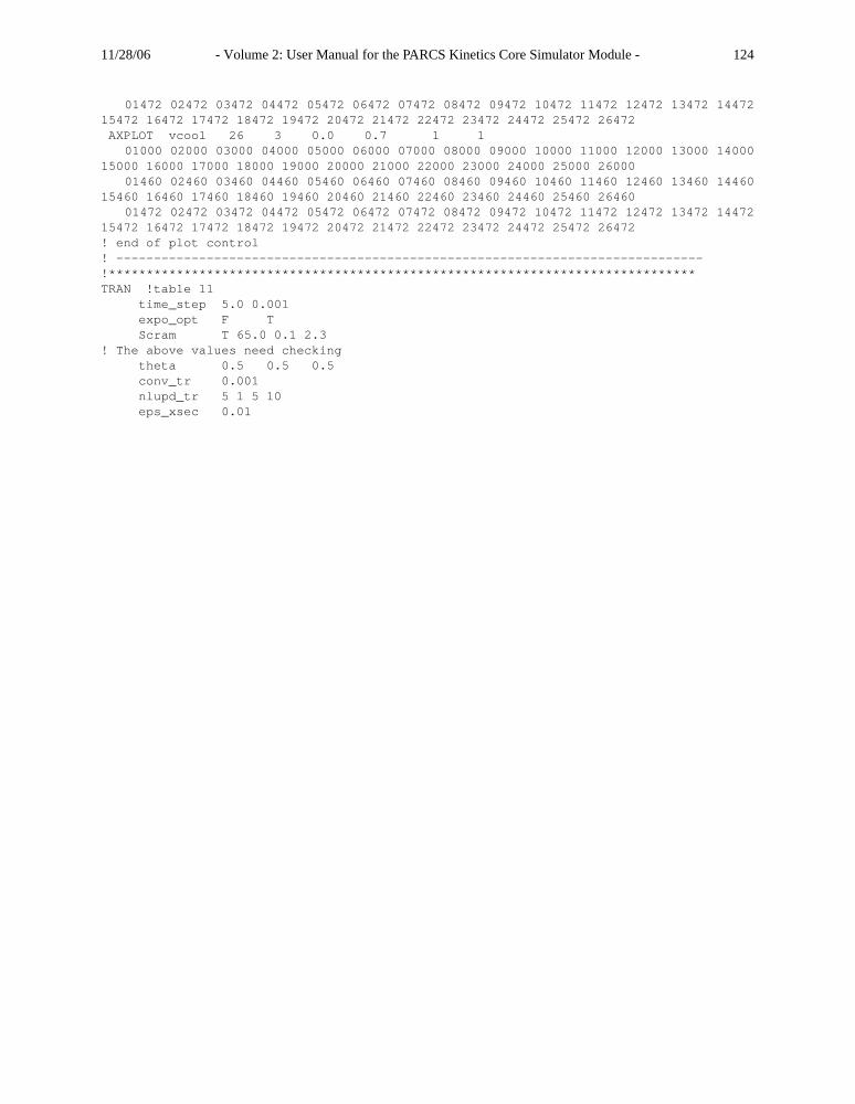
11/28/06 - Volume 2: User Manual for the PARCS Kinetics Core Simulator Module - 124
01472 02472 03472 04472 05472 06472 07472 08472 09472 10472 11472 12472 13472 1447215472 16472 17472 18472 19472 20472 21472 22472 23472 24472 25472 26472 AXPLOT vcool 26 3 0.0 0.7 1 1 01000 02000 03000 04000 05000 06000 07000 08000 09000 10000 11000 12000 13000 1400015000 16000 17000 18000 19000 20000 21000 22000 23000 24000 25000 26000 01460 02460 03460 04460 05460 06460 07460 08460 09460 10460 11460 12460 13460 1446015460 16460 17460 18460 19460 20460 21460 22460 23460 24460 25460 26460 01472 02472 03472 04472 05472 06472 07472 08472 09472 10472 11472 12472 13472 1447215472 16472 17472 18472 19472 20472 21472 22472 23472 24472 25472 26472! end of plot control! ------------------------------------------------------------------------------!******************************************************************************TRAN !table 11 time_step 5.0 0.001 expo_opt F T Scram T 65.0 0.1 2.3! The above values need checking theta 0.5 0.5 0.5 conv_tr 0.001 nlupd_tr 5 1 5 10 eps_xsec 0.01
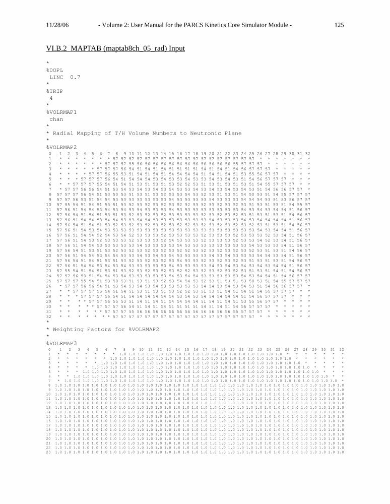
11/28/06 - Volume 2: User Manual for the PARCS Kinetics Core Simulator Module - 125
VI.B.2 MAPTAB (maptab8ch_05_rad) Input
*%DOPL LINC 0.7*%TRIP 4*%VOLRMAP1 chan** Radial Mapping of T/H Volume Numbers to Neutronic Plane*%VOLRMAP2 0 1 2 3 4 5 6 7 8 9 10 11 12 13 14 15 16 17 18 19 20 21 22 23 24 25 26 27 28 29 30 31 32 1 * * * * * * * 57 57 57 57 57 57 57 57 57 57 57 57 57 57 57 57 57 57 * * * * * * * 2 * * * * * * 57 57 57 55 56 56 56 56 56 56 56 56 56 56 56 56 55 57 57 57 * * * * * * 3 * * * * * 57 57 57 56 54 51 54 51 54 51 51 51 51 54 51 54 51 54 56 57 57 57 * * * * * 4 * * * * 57 57 56 55 53 51 54 51 54 51 54 54 54 54 51 54 51 54 51 53 55 56 57 57 * * * * 5 * * * 57 57 57 56 54 51 54 54 54 53 54 53 53 54 53 53 54 53 54 53 51 54 56 57 57 57 * * * 6 * * 57 57 57 55 54 51 54 51 53 51 53 51 53 52 52 53 51 53 51 53 51 53 51 54 55 57 57 57 * * 7 * 57 57 56 56 54 51 53 54 53 54 53 54 53 54 53 53 54 53 54 53 54 53 54 53 51 54 56 56 57 57 * 8 57 57 57 56 54 51 53 50 53 51 53 51 53 52 53 53 54 53 52 53 51 53 51 54 50 53 51 54 55 57 57 57 9 57 57 56 53 51 54 54 53 53 53 53 53 53 53 54 53 53 53 53 54 53 53 53 54 54 54 53 51 53 56 57 57 10 57 55 54 51 54 51 53 51 53 52 53 52 53 52 53 52 52 53 52 53 52 53 52 53 51 53 51 53 51 54 55 57 11 57 56 51 54 54 53 54 53 54 53 54 53 53 53 54 53 53 53 53 53 53 53 53 54 53 54 53 54 54 51 56 57 12 57 56 54 51 54 51 53 51 53 52 53 52 53 52 53 53 53 53 52 53 52 53 52 53 51 53 51 53 51 54 56 57 13 57 56 51 54 54 53 54 54 53 53 54 54 53 53 53 53 53 53 53 54 53 53 53 54 53 54 54 54 54 51 56 57 14 57 56 54 51 54 51 53 52 53 52 53 52 53 52 53 52 52 53 52 53 52 53 52 53 52 53 51 53 51 54 56 57 15 57 56 51 54 53 54 53 53 53 53 53 53 53 53 53 53 53 53 53 53 53 53 53 53 53 54 53 54 54 51 56 57 16 57 56 51 54 54 52 54 53 54 52 53 53 53 52 53 53 53 53 52 53 53 53 52 53 53 53 52 53 54 51 56 57 17 57 56 51 54 53 52 53 53 53 52 53 53 53 52 54 53 53 53 52 53 53 53 52 53 53 54 52 53 54 51 56 57 18 57 56 51 54 54 53 53 53 53 53 54 53 53 53 53 54 53 53 53 53 53 53 53 53 54 53 53 53 54 51 56 57 19 57 56 54 51 53 51 53 52 53 52 53 52 53 52 53 52 52 53 52 53 52 53 52 53 52 53 51 53 51 54 56 57 20 57 56 51 54 54 53 54 54 53 53 54 53 54 53 54 53 53 53 53 54 53 54 53 53 53 54 54 53 54 51 56 57 21 57 56 54 51 54 51 53 51 53 52 53 52 53 52 53 54 53 53 52 53 52 53 52 53 51 53 51 53 51 54 56 57 22 57 56 51 54 54 53 54 53 54 53 53 53 53 53 54 53 53 53 53 54 53 54 53 54 53 54 53 54 54 51 56 57 23 57 55 54 51 54 51 53 51 53 52 53 52 53 52 53 52 52 53 52 53 52 53 52 53 51 53 51 54 51 54 56 57 24 57 57 56 53 51 54 54 53 54 53 53 53 53 53 54 53 54 54 53 53 53 53 53 54 53 54 54 51 54 56 57 57 25 57 57 57 55 54 51 53 50 53 51 53 51 53 52 53 54 54 53 52 53 51 53 51 53 50 53 51 54 55 57 57 57 26 * 57 57 56 56 54 51 53 54 53 54 53 54 53 53 53 53 53 54 54 53 54 53 54 53 51 54 56 56 57 57 * 27 * * 57 57 57 55 54 51 54 51 53 51 53 51 53 52 52 53 51 53 51 54 51 54 51 54 55 57 57 57 * * 28 * * * 57 57 57 56 54 51 54 54 54 54 54 54 53 54 53 54 54 54 54 54 51 54 56 57 57 57 * * * 29 * * * * 57 57 56 55 53 51 54 51 54 51 54 54 54 54 51 54 51 54 51 53 55 56 57 57 * * * * 30 * * * * * 57 57 57 56 54 51 54 51 54 51 51 51 51 54 51 54 51 54 56 57 57 57 * * * * * 31 * * * * * * 57 57 57 55 56 56 56 56 56 56 56 56 56 56 56 56 55 57 57 57 * * * * * * 32 * * * * * * * 57 57 57 57 57 57 57 57 57 57 57 57 57 57 57 57 57 57 * * * * * * * ** Weighting Factors for %VOLRMAP2*%VOLRMAP3 0 1 2 3 4 5 6 7 8 9 10 11 12 13 14 15 16 17 18 19 20 21 22 23 24 25 26 27 28 29 30 31 32 1 * * * * * * * 1.0 1.0 1.0 1.0 1.0 1.0 1.0 1.0 1.0 1.0 1.0 1.0 1.0 1.0 1.0 1.0 1.0 1.0 * * * * * * * 2 * * * * * * 1.0 1.0 1.0 1.0 1.0 1.0 1.0 1.0 1.0 1.0 1.0 1.0 1.0 1.0 1.0 1.0 1.0 1.0 1.0 1.0 * * * * * * 3 * * * * * 1.0 1.0 1.0 1.0 1.0 1.0 1.0 1.0 1.0 1.0 1.0 1.0 1.0 1.0 1.0 1.0 1.0 1.0 1.0 1.0 1.0 1.0 * * * * * 4 * * * * 1.0 1.0 1.0 1.0 1.0 1.0 1.0 1.0 1.0 1.0 1.0 1.0 1.0 1.0 1.0 1.0 1.0 1.0 1.0 1.0 1.0 1.0 1.0 1.0 * * * * 5 * * * 1.0 1.0 1.0 1.0 1.0 1.0 1.0 1.0 1.0 1.0 1.0 1.0 1.0 1.0 1.0 1.0 1.0 1.0 1.0 1.0 1.0 1.0 1.0 1.0 1.0 1.0 * * * 6 * * 1.0 1.0 1.0 1.0 1.0 1.0 1.0 1.0 1.0 1.0 1.0 1.0 1.0 1.0 1.0 1.0 1.0 1.0 1.0 1.0 1.0 1.0 1.0 1.0 1.0 1.0 1.0 1.0 * * 7 * 1.0 1.0 1.0 1.0 1.0 1.0 1.0 1.0 1.0 1.0 1.0 1.0 1.0 1.0 1.0 1.0 1.0 1.0 1.0 1.0 1.0 1.0 1.0 1.0 1.0 1.0 1.0 1.0 1.0 1.0 * 8 1.0 1.0 1.0 1.0 1.0 1.0 1.0 1.0 1.0 1.0 1.0 1.0 1.0 1.0 1.0 1.0 1.0 1.0 1.0 1.0 1.0 1.0 1.0 1.0 1.0 1.0 1.0 1.0 1.0 1.0 1.0 1.0 9 1.0 1.0 1.0 1.0 1.0 1.0 1.0 1.0 1.0 1.0 1.0 1.0 1.0 1.0 1.0 1.0 1.0 1.0 1.0 1.0 1.0 1.0 1.0 1.0 1.0 1.0 1.0 1.0 1.0 1.0 1.0 1.010 1.0 1.0 1.0 1.0 1.0 1.0 1.0 1.0 1.0 1.0 1.0 1.0 1.0 1.0 1.0 1.0 1.0 1.0 1.0 1.0 1.0 1.0 1.0 1.0 1.0 1.0 1.0 1.0 1.0 1.0 1.0 1.011 1.0 1.0 1.0 1.0 1.0 1.0 1.0 1.0 1.0 1.0 1.0 1.0 1.0 1.0 1.0 1.0 1.0 1.0 1.0 1.0 1.0 1.0 1.0 1.0 1.0 1.0 1.0 1.0 1.0 1.0 1.0 1.012 1.0 1.0 1.0 1.0 1.0 1.0 1.0 1.0 1.0 1.0 1.0 1.0 1.0 1.0 1.0 1.0 1.0 1.0 1.0 1.0 1.0 1.0 1.0 1.0 1.0 1.0 1.0 1.0 1.0 1.0 1.0 1.013 1.0 1.0 1.0 1.0 1.0 1.0 1.0 1.0 1.0 1.0 1.0 1.0 1.0 1.0 1.0 1.0 1.0 1.0 1.0 1.0 1.0 1.0 1.0 1.0 1.0 1.0 1.0 1.0 1.0 1.0 1.0 1.014 1.0 1.0 1.0 1.0 1.0 1.0 1.0 1.0 1.0 1.0 1.0 1.0 1.0 1.0 1.0 1.0 1.0 1.0 1.0 1.0 1.0 1.0 1.0 1.0 1.0 1.0 1.0 1.0 1.0 1.0 1.0 1.015 1.0 1.0 1.0 1.0 1.0 1.0 1.0 1.0 1.0 1.0 1.0 1.0 1.0 1.0 1.0 1.0 1.0 1.0 1.0 1.0 1.0 1.0 1.0 1.0 1.0 1.0 1.0 1.0 1.0 1.0 1.0 1.016 1.0 1.0 1.0 1.0 1.0 1.0 1.0 1.0 1.0 1.0 1.0 1.0 1.0 1.0 1.0 1.0 1.0 1.0 1.0 1.0 1.0 1.0 1.0 1.0 1.0 1.0 1.0 1.0 1.0 1.0 1.0 1.017 1.0 1.0 1.0 1.0 1.0 1.0 1.0 1.0 1.0 1.0 1.0 1.0 1.0 1.0 1.0 1.0 1.0 1.0 1.0 1.0 1.0 1.0 1.0 1.0 1.0 1.0 1.0 1.0 1.0 1.0 1.0 1.018 1.0 1.0 1.0 1.0 1.0 1.0 1.0 1.0 1.0 1.0 1.0 1.0 1.0 1.0 1.0 1.0 1.0 1.0 1.0 1.0 1.0 1.0 1.0 1.0 1.0 1.0 1.0 1.0 1.0 1.0 1.0 1.019 1.0 1.0 1.0 1.0 1.0 1.0 1.0 1.0 1.0 1.0 1.0 1.0 1.0 1.0 1.0 1.0 1.0 1.0 1.0 1.0 1.0 1.0 1.0 1.0 1.0 1.0 1.0 1.0 1.0 1.0 1.0 1.020 1.0 1.0 1.0 1.0 1.0 1.0 1.0 1.0 1.0 1.0 1.0 1.0 1.0 1.0 1.0 1.0 1.0 1.0 1.0 1.0 1.0 1.0 1.0 1.0 1.0 1.0 1.0 1.0 1.0 1.0 1.0 1.021 1.0 1.0 1.0 1.0 1.0 1.0 1.0 1.0 1.0 1.0 1.0 1.0 1.0 1.0 1.0 1.0 1.0 1.0 1.0 1.0 1.0 1.0 1.0 1.0 1.0 1.0 1.0 1.0 1.0 1.0 1.0 1.022 1.0 1.0 1.0 1.0 1.0 1.0 1.0 1.0 1.0 1.0 1.0 1.0 1.0 1.0 1.0 1.0 1.0 1.0 1.0 1.0 1.0 1.0 1.0 1.0 1.0 1.0 1.0 1.0 1.0 1.0 1.0 1.023 1.0 1.0 1.0 1.0 1.0 1.0 1.0 1.0 1.0 1.0 1.0 1.0 1.0 1.0 1.0 1.0 1.0 1.0 1.0 1.0 1.0 1.0 1.0 1.0 1.0 1.0 1.0 1.0 1.0 1.0 1.0 1.0

11/28/06 - Volume 2: User Manual for the PARCS Kinetics Core Simulator Module - 126
24 1.0 1.0 1.0 1.0 1.0 1.0 1.0 1.0 1.0 1.0 1.0 1.0 1.0 1.0 1.0 1.0 1.0 1.0 1.0 1.0 1.0 1.0 1.0 1.0 1.0 1.0 1.0 1.0 1.0 1.0 1.0 1.025 1.0 1.0 1.0 1.0 1.0 1.0 1.0 1.0 1.0 1.0 1.0 1.0 1.0 1.0 1.0 1.0 1.0 1.0 1.0 1.0 1.0 1.0 1.0 1.0 1.0 1.0 1.0 1.0 1.0 1.0 1.0 1.026 * 1.0 1.0 1.0 1.0 1.0 1.0 1.0 1.0 1.0 1.0 1.0 1.0 1.0 1.0 1.0 1.0 1.0 1.0 1.0 1.0 1.0 1.0 1.0 1.0 1.0 1.0 1.0 1.0 1.0 1.0 *27 * * 1.0 1.0 1.0 1.0 1.0 1.0 1.0 1.0 1.0 1.0 1.0 1.0 1.0 1.0 1.0 1.0 1.0 1.0 1.0 1.0 1.0 1.0 1.0 1.0 1.0 1.0 1.0 1.0 * *28 * * * 1.0 1.0 1.0 1.0 1.0 1.0 1.0 1.0 1.0 1.0 1.0 1.0 1.0 1.0 1.0 1.0 1.0 1.0 1.0 1.0 1.0 1.0 1.0 1.0 1.0 1.0 * * *29 * * * * 1.0 1.0 1.0 1.0 1.0 1.0 1.0 1.0 1.0 1.0 1.0 1.0 1.0 1.0 1.0 1.0 1.0 1.0 1.0 1.0 1.0 1.0 1.0 1.0 * * * *30 * * * * * 1.0 1.0 1.0 1.0 1.0 1.0 1.0 1.0 1.0 1.0 1.0 1.0 1.0 1.0 1.0 1.0 1.0 1.0 1.0 1.0 1.0 1.0 * * * * *31 * * * * * * 1.0 1.0 1.0 1.0 1.0 1.0 1.0 1.0 1.0 1.0 1.0 1.0 1.0 1.0 1.0 1.0 1.0 1.0 1.0 1.0 * * * * * *32 * * * * * * * 1.0 1.0 1.0 1.0 1.0 1.0 1.0 1.0 1.0 1.0 1.0 1.0 1.0 1.0 1.0 1.0 1.0 1.0 * * * * * * *

11/28/06 - Volume 2: User Manual for the PARCS Kinetics Core Simulator Module - 127
VI.C VVER1000 Rod Ejection Benchmark
!******************************************************************************CASEID vv1kre VVER1K Rod Ejection Benchmark - Refernce Calc. Options!******************************************************************************CNTL core_power 10.0 !in % bank_pos 282.4 353.0 353.0 353.0 353.0 353.0 353.0 0. 0. ppm 1000. search ppm transient T! input iteration planar adj! edit table power pin reac print_opt T F F F T! fdbk flux planar! rho precurs flux Xe T/H print_opt F F F F F
!******************************************************************************PARAM! no parameters are specified, all defaults conv_ss 1.e-6 1.e-5 1.e-3
!******************************************************************************XSEC func_type 12 ! special xsec for VVER1K
!Delayed Neutron Precurosor Data!-------------------------------------------------------------------------------- dnp_ngrp 6 kin_comp 1 1 -4 !Compostions that this set applies dnp_lambda 0.0128 0.0315 0.125 0.325 1.55 4.5 !decay constants dnp_beta 1.566e-4 1.028e-3 9.442e-4 1.995e-3 6.538e-4 2.224e-4 !beta neut_velo 1.98e7 6.15e5 ! Neutron Velocities (cm/sec)
!******************************************************************************GEOMHEX geo_dim 7 15 !nring, nz rad_conf 360 !full rotation symmetry 3 3 3 3 3 3 3 4 2 1 2 1 2 4 3 3 2 1 2 1 1 2 1 2 3 3 1 2 1 1 1 1 1 2 1 3 3 2 1 1 2 1 1 2 1 1 2 3 3 1 1 1 1 1 2 1 1 1 1 1 3 3 2 2 1 1 2 1 1 2 1 1 2 2 3 4 1 1 2 1 1 1 1 1 2 1 1 4 3 2 2 1 1 2 1 1 2 1 1 2 2 3 3 1 1 1 1 1 2 1 1 1 1 1 3 3 2 1 1 2 1 1 2 1 1 2 3 3 1 2 1 1 1 1 1 2 1 3 3 2 1 2 1 1 2 1 2 3 3 4 2 1 2 1 2 4 3 3 3 3 3 3 3
grid_hex 23.6 !flat-to-flat distance (cm)

11/28/06 - Volume 2: User Manual for the PARCS Kinetics Core Simulator Module - 128
grid_z 15*23.533333 assy_type 1 15*1 assy_type 2 15*2 assy_type 3 15*3 assy_type 4 15*4 albedo_r 0.1468 0.0831 albedo_zb 0.1699 0.0061 albedo_zt 0.1670 0.0802
cr_axinfo 0.0 1.0 ! step size is 1cm bank_conf 0 0 0 0 0 0 0 0 0 0 9 0 0 0 0 0 0 0 0 0 0 0 0 0 0 0 0 0 0 0 0 0 0 0 0 0 0 9 0 0 1 0 0 1 0 0 8 0 0 0 0 0 0 0 0 0 0 0 0 0 0 0 0 0 0 0 0 0 0 0 0 0 0 0 0 0 0 0 1 0 0 0 0 0 1 0 0 0 0 0 0 0 0 0 0 0 0 0 0 0 0 0 0 0 0 0 0 0 0 0 0 0 0 0 0 0 8 0 0 1 0 0 1 0 0 8 0 0 0 0 0 0 0 0 0 0 0 0 0 0 0 0 0 0 0 0 0 0 0 0 0 0 9 0 0 0 0 0 0 0 0 0 0
!******************************************************************************TH n_pingt 312 19 !npin,ngt fa_powpit 18.4049 21.962275 !assembly power(Mw) and pitch(cm) pin_dim 3.765 4.55 0.69 6.3 !pin radii, rs,rw,tw, and rgt in mm flow_cond 288.0 112.426 !tin,cmfrfa(Kg/sec) gamma_frac 0.0 !direc heating fraction hgap 3157.9 !hgap(w/M^2-C) n_ring 6 !number of meshes in pellet !******************************************************************************TRAN time_step 5.00 0.01 1.0 10.0 !tend,delt0,tswitch,texpand move_bank 9 0.0 0.0 0.1 353.0 conv_tr 0.00001 !eps_r2 eps_xsec 0.0001.
VI.D PARCS model for PBMR-268 steady-state neutronics benchmark problem.
CASEID PBMR CASE N-1 (Cylindrical Coordinate)!******************************************************************************CNTL th_fdbk F! input iteration planar adj! edit table power pin reac print_opt T T T F F! fdbk flux planar

11/28/06 - Volume 2: User Manual for the PARCS Kinetics Core Simulator Module - 129
! rho precurs flux Xe T/H print_opt F T T F F! radial radial! power flux print_opt F F T T F
!******************************************************************************PARAM n_iters 20 500 nlupd_ss 5 5 1 nodal_kern fmfd
conv_ss 1.0e-6 1.e-6 1.e-6 0.001 !keff,globfs,locfs,tempf wielandt 1.0e+30 1.0e+30 1.0 !turnoff wielandt
eps_erf 0.00001 !default 0.005 try to change this value eps_anm 1e+50 !
!******************************************************************************XSEC file XSEC_PBMR DDDC 7 0.1 0.5!******************************************************************************FMFD ref_cond 0.0 296.85 0.7295 626.85 !ppm, Tm in C, rho in gm/cc, Tf in C ! for TH / depl, transient dnp_ngrp 6 geninf 2 1 1 1 1 1 !pinx#/FA piny#/FA #/pin ... ! mmx mmy nrefine mmz mmxth mmyth method 1 3 !order(1:diff,3:sp3) naccel(1:cmr,2:cmfd)
file FMFD_PBMR20x20!******************************************************************************GEOM geo_dim 11 1 22 !nasyx,nasyy,nz coordinate 2 !2=cylinder, default=.not. cylinder rad_conf 1 2 2 2 2 1 1 1 1 1 1 grid_r 78.6 32.3 24.8 20.9 18.4 6.0 13.0 21.0 20.0 15.0 25.0 ! grid_r in cylinder(cm) neutmesh_r 1 1 1 1 1 1 1 1 1 1 1 grid_theta 1*3.0 ! grid_theta in cylinder (degree)

11/28/06 - Volume 2: User Manual for the PARCS Kinetics Core Simulator Module - 130
neutmesh_theta 1*1 grid_z 2*50.0 25.0 17*50.0 2*50.0 boun_cond 0 2 0 0 2 2 !ibcw,ibce,ibcn,ibcs,ibcb,ibct Planar_Reg 1 8 8 8 8 8 9 9 9 16 9 17 Planar_Reg 2 8 8 8 8 8 9 9 9 16 9 17 . . . Planar_Reg 22 13 13 13 13 13 9 9 9 16 9 17
PR_Assign 1 2 3 4 5 6 7 8 9 10 11 12 13 14 15 16 17 18 19 20 21 22 cr_axinfo 100.0 38.1 !fully inserted position and step size

11/28/06 - Volume 2: User Manual for the PARCS Kinetics Core Simulator Module - 131
VII. SAMPLE OUTPUTS
VII.A OECD MSLB Benchmark
VII.A.1 Steady State Output
PARCSPARCSPARCSPARCSPARCSPARCSPARCSPARCSPARCSPARCSPARCSPARCSPARCSPARCS
PPPPPPP A RRRRRRR CCCCC SSSSS PPPPPPPPP AAA RRRRRRRRR CCCCCCCCC SSSSSSSSS PPP PPPP AA AA RRR RRRR CCC CC SSS SSS PPP PPPP AA AA RRR RRRR CCC C SSS SS PPP PPPP AA AA RRR RRRR CCC SSS PPPPPPPPP AA AA RRRRRRRRR CCC SSSS PPPPPPP AA AA RRRRRRR CCC SSSSSSS PPP AA AA RRR RR CCC SSSSSSS PPP AAAAAAAAAAA RRR RR CCC SSSS PPP AA AA RRR RR CCC SSS PPP AA AA RRR RR CCC C SS SSS PPP AA AA RRR RR CCC CCC SSS SSS PPP AA AA RRR RR CCCCCCCCC SSSSSSSSS PPP AA AA RRR RR CCCCC SSSSS
(Purdue Advanced Reactor Core Simulator)
NRC - V1.17 Mod0
PARCSPARCSPARCSPARCSPARCSPARCSPARCSPARCSPARCSPARCSPARCSPARCSPARCSPARCS...... ================================================ Steady State Eigenvalue Calculation Results ================================================ Itr Nin k-eff Global F.S. Local F.S. Dom. R PPM ------------------------------------------------------------------------------- 1 1 1.0085264 F 1.9895E-01 F 1.1835E+00 F 10.0000 5.00 2 1 1.0107931 F 9.7897E-02 F 4.5330E-01 F 0.4988 5.00 3 1 1.0133206 F 1.0210E-01 F 1.8412E-01 F 1.1086 5.00 4 1 1.0148231 F 9.1280E-02 F 1.4893E-01 F 0.9401 5.00 5 1 1.0154511 F 6.6549E-02 F 1.3770E-01 F 0.7483 5.00 00:08.91 Nodal update... 1, NEM= 0, ANM=21437 00:08.95 @0.00E+00 s, k-eff= 1.015451 , Tout= 312.85 C, Tfmax= 648.73 C Restart advancement: 0 written at time: 0.00000100 s

11/28/06 - Volume 2: User Manual for the PARCS Kinetics Core Simulator Module - 132
Itr Nin k-eff Global F.S. Local F.S. Dom. R PPM ------------------------------------------------------------------------------- 6 1 1.0080465 F 1.2552E-01 F 3.7788E-01 F 1.8203 5.00 00:09.42 @1.00E-06 s, k-eff= 1.008046 , Tout= 312.85 C, Tfmax= 648.73 C ...... Itr Nin k-eff Global F.S. Local F.S. Dom. R PPM ------------------------------------------------------------------------------- 120 1 1.0048973 F 2.2386E-05 T 3.5597E-05 T 0.7584 5.00 00:35.59 @ 959.989 s, k-eff= 1.004897 , Tout= 320.47 C, Tfmax= 631.23 C PDMR: Cleaning up PDMR Memory... All done. Leaving PDMR...Restart advancement: 20 written at time: 1001.98928193 s Itr Nin k-eff Global F.S. Local F.S. Dom. R PPM ------------------------------------------------------------------------------- 121 1 1.0048935 F 5.0072E-05 F 6.6925E-05 T 2.2367 5.00 00:36.11 @1001.989 s, k-eff= 1.004893 , Tout= 320.48 C, Tfmax= 631.24 C Time: 0.000 K-Effective: 1.004893 Boron Conc: 5.00 Core Power Level: 1.000000E+00...... Number of CMFD/Nodal/TH Updates and Inners: 3593 18 0 121
Time for Init. 8.125 CMFD 17.641 Nodal 4.422 T/H 10.422 Xsec 3.719 Decusping 0.000 Precond. 0.000 Pin Power 0.000 ----- Total 36.203

11/28/06 - Volume 2: User Manual for the PARCS Kinetics Core Simulator Module - 133
VII.A.2 Transient Output
PARCSPARCSPARCSPARCSPARCSPARCSPARCSPARCSPARCSPARCSPARCSPARCSPARCSPARCS
PPPPPPP A RRRRRRR CCCCC SSSSS PPPPPPPPP AAA RRRRRRRRR CCCCCCCCC SSSSSSSSS PPP PPPP AA AA RRR RRRR CCC CC SSS SSS PPP PPPP AA AA RRR RRRR CCC C SSS SS PPP PPPP AA AA RRR RRRR CCC SSS PPPPPPPPP AA AA RRRRRRRRR CCC SSSS PPPPPPP AA AA RRRRRRR CCC SSSSSSS PPP AA AA RRR RR CCC SSSSSSS PPP AAAAAAAAAAA RRR RR CCC SSSS PPP AA AA RRR RR CCC SSS PPP AA AA RRR RR CCC C SS SSS PPP AA AA RRR RR CCC CCC SSS SSS PPP AA AA RRR RR CCCCCCCCC SSSSSSSSS PPP AA AA RRR RR CCCCC SSSSS
(Purdue Advanced Reactor Core Simulator)
NRC - V1.17 Mod0
PARCSPARCSPARCSPARCSPARCSPARCSPARCSPARCSPARCSPARCSPARCSPARCSPARCSPARCS......=================================================================== Performing Transient Calculation...=================================================================== 00:13.45 @ 0.000 s, P= 1.000E+02 %, Tout= 320.5 Tf= 631.2 C rho= 0.0 cRestart advancement: 21 written at time: 0.01000000 s Core condition changes which initiate transient Time: 0.010 Boron : not changed 00:14.73 @ 0.010 s, P= 1.000E+02 %, Tout= 320.5 Tf= 631.2 C rho= 0.0 c Time: 0.010 Reactivity($): 0.000046 Core beta : 0.005211 Boron Conc: 5.00 Core Power Level: 1.000008E+00 Enthalpy Rise 0.01000 149 23 289.84 0.000 0.000 1.4319 1.43191.0000 Assembly Power Distribution

11/28/06 - Volume 2: User Manual for the PARCS Kinetics Core Simulator Module - 134
#.#### box power 1 2 3 4 5 6 7 8 9 10 11 12 13 14 15 16 2 0.3998 0.4573 0.3982 0.4574 0.399 3 0.4628 0.6982 1.1046 1.2074 0.8332 1.2076 1.1049 0.6985 0.4631 4 0.6073 1.0977 0.9472 1.3039 1.0849 1.3005 1.0852 1.3044 0.9476 1.0984 0.6078 5 0.4614 1.0962 1.0601 1.3004 1.0447 1.3203 1.0399 1.3207 1.0452 1.3012 1.0611 1.0975 0.4621 6 0.6924 0.9446 1.2994 1.0566 1.3086 1.0573 1.2975 1.0577 1.3096 1.0577 1.3012 0.9462 0.6938 7 0.3946 1.0925 1.3007 1.0450 1.3079 1.0360 1.2713 1.0439 1.2721 1.0372 1.3101 1.0472 1.3039 1.0956 0.3959 8 0.4509 1.1930 1.0815 1.3198 1.0550 1.2689 0.9961 1.2320 0.9970 1.2712 1.0579 1.3240 1.0853 1.1975 0.4527 9 0.3922 0.8226 1.2948 1.0380 1.2925 1.0401 1.2291 0.8747 1.2309 1.0432 1.2978 1.0427 1.3013 0.8271 0.3944 10 0.4497 1.1895 1.0786 1.3164 1.0523 1.2659 0.9942 1.2304 0.9966 1.2719 1.0597 1.3264 1.0872 1.1988 0.4532 11 0.3932 1.0879 1.2951 1.0406 1.3026 1.0322 1.2677 1.0425 1.2727 1.0404 1.3175 1.0551 1.3119 1.1005 0.3974 12 0.6889 0.9395 1.2925 1.0514 1.3028 1.0539 1.2958 1.0597 1.3173 1.0713 1.3249 0.9614 0.7020 13 0.4587 1.0894 1.0537 1.2931 1.0397 1.3157 1.0387 1.3241 1.0544 1.3256 1.1125 1.1267 0.4714 14 0.6034 1.0907 0.9417 1.2972 1.0811 1.2991 1.0884 1.3147 0.9639 1.1281 0.6253 15 0.4600 0.6941 1.0987 1.2028 0.8326 1.2107 1.1122 0.7080 0.4728 16 0.3978 0.4557 0.3980 0.4586 0.4022 Maximum Pos. Maximum Value ( 13, 10 ) 1.3264 Axial Power Distribution Height(cm) Power Plane Mesh from bottom Number (cm) 7.44 0.745 2 14.88 17.23 0.873 3 4.71 24.68 0.961 4 10.17 37.20 1.017 5 14.88 52.08 1.042 6 14.88 66.96 1.045 7 14.88 81.84 1.045 8 14.88 96.72 1.040 9 14.88 111.60 1.035 10 14.88 126.48 1.031 11 14.88 141.36 1.037 12 14.88 156.24 1.032 13 14.88 171.12 1.024 14 14.88 186.00 1.015 15 14.88 200.88 1.008 16 14.88 215.76 1.008 17 14.88 230.64 1.020 18 14.88 245.52 1.024 19 14.88 260.40 1.028 20 14.88 275.28 1.035 21 14.88 290.16 1.053 22 14.88 305.04 1.058 23 14.88 319.92 1.031 24 14.88 333.49 0.946 25 12.27 340.93 0.846 26 2.61 349.68 0.766 27 14.88 Maximum Pos. Maximum Value 23 1.0576
Fq (Pin) 1.4319......Restart advancement: 34 written at time: 100.15899185 s
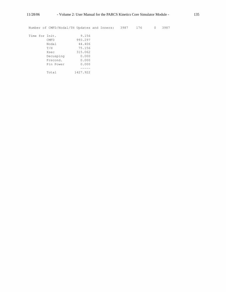
11/28/06 - Volume 2: User Manual for the PARCS Kinetics Core Simulator Module - 135
Number of CMFD/Nodal/TH Updates and Inners: 3987 176 0 3987
Time for Init. 9.156 CMFD 993.297 Nodal 44.406 T/H 75.156 Xsec 315.062 Decusping 0.000 Precond. 0.000 Pin Power 0.000 ----- Total 1427.922

11/28/06 - Volume 2: User Manual for the PARCS Kinetics Core Simulator Module - 136
VII.B BWR Peach Bottom Turbine Trip Benchmark
VII.B.1 Steady State Output
PARCSPARCSPARCSPARCSPARCSPARCSPARCSPARCSPARCSPARCSPARCSPARCSPARCSPARCS
PPPPPPP A RRRRRRR CCCCC SSSSS PPPPPPPPP AAA RRRRRRRRR CCCCCCCCC SSSSSSSSS PPP PPPP AA AA RRR RRRR CCC CC SSS SSS PPP PPPP AA AA RRR RRRR CCC C SSS SS PPP PPPP AA AA RRR RRRR CCC SSS PPPPPPPPP AA AA RRRRRRRRR CCC SSSS PPPPPPP AA AA RRRRRRR CCC SSSSSSS PPP AA AA RRR RR CCC SSSSSSS PPP AAAAAAAAAAA RRR RR CCC SSSS PPP AA AA RRR RR CCC SSS PPP AA AA RRR RR CCC C SS SSS PPP AA AA RRR RR CCC CCC SSS SSS PPP AA AA RRR RR CCCCCCCCC SSSSSSSSS PPP AA AA RRR RR CCCCC SSSSS
(Purdue Advanced Reactor Core Simulator)
NRC - V1.17 Mod0
PARCSPARCSPARCSPARCSPARCSPARCSPARCSPARCSPARCSPARCSPARCSPARCSPARCSPARCS...... ================================================ Steady State Eigenvalue Calculation Results ================================================ PDMR: Receiving Time-Dependent TRACE Buffer... PDMR: Receiving Permuted TRACE Vector... Itr Nin k-eff Global F.S. Local F.S. Dom. R PPM ------------------------------------------------------------------------------- 1 2 1.0100249 F 3.4064E-01 F 3.1788E+00 F 10.0000 0.00 2 5 1.0201937 F 3.4349E-01 F 8.1428E-01 F 1.2646 0.00 3 4 1.0207202 F 7.0602E-02 F 4.6712E-01 F 0.2403 0.00 03:50.38 Nodal update... 1, NEM=12504, ANM=61208 03:50.70 @0.00E+00 s, k-eff= 1.020720 , Tout= 286.85 C, Tfmax= 291.85 C PDMR: Sending Time-Depedendent PARCS Buffer... PDMR: Sending Unpermuted PARCS Vector... PDMR: Receiving Time-Dependent TRACE Buffer...

11/28/06 - Volume 2: User Manual for the PARCS Kinetics Core Simulator Module - 137
PDMR: Receiving Permuted TRACE Vector... Restart advancement: 0 written at time: 0.00000100 s Itr Nin k-eff Global F.S. Local F.S. Dom. R PPM ------------------------------------------------------------------------------- 4 3 1.0153525 F 1.3621E-01 F 7.1890E-01 F 1.8357 0.00 03:55.22 @1.00E-06 s, k-eff= 1.015353 , Tout= 286.85 C, Tfmax= 291.93 C PDMR: Sending Time-Depedendent PARCS Buffer... PDMR: Sending Unpermuted PARCS Vector... PDMR: Receiving Time-Dependent TRACE Buffer... PDMR: Receiving Permuted TRACE Vector... . . . . . . Itr Nin k-eff Global F.S. Local F.S. Dom. R PPM ------------------------------------------------------------------------------- 120 3 1.0017572 T 2.6570E-05 F 8.7476E-05 T 1.2100 0.00 10:09.52 @ 45.678 s, k-eff= 1.001757 , Tout= 283.77 C, Tfmax= 628.22 C PDMR: Sending Time-Depedendent PARCS Buffer... PDMR: Sending Unpermuted PARCS Vector... PDMR: Receiving Time-Dependent TRACE Buffer... PDMR: Receiving Permuted TRACE Vector... PDMR: Cleaning up PDMR Memory... All done. Leaving PDMR...Restart advancement: 1 written at time: 46.00049692 s Itr Nin k-eff Global F.S. Local F.S. Dom. R PPM ------------------------------------------------------------------------------- 121 3 1.0017571 T 1.0509E-05 F 2.7272E-05 T 0.3955 0.00 10:13.50 @ 46.000 s, k-eff= 1.001757 , Tout= 283.77 C, Tfmax= 628.22 C Time: 0.000 K-Effective: 1.001757 Boron Conc: 0.00 Core Power Level: 6.158520E-01.... Number of CMFD/Nodal/TH Updates and Inners: 3824 33 0 430
Time for Init. 221.641 CMFD 268.469 Nodal 74.922 T/H 238.000 Xsec 32.453 Decusping 0.000 Precond. 0.000 Pin Power 0.000 ----- Total 613.844

11/28/06 - Volume 2: User Manual for the PARCS Kinetics Core Simulator Module - 138
VII.C VVER1000 Rod Ejection Benchmark
PARCSPARCSPARCSPARCSPARCSPARCSPARCSPARCSPARCSPARCSPARCSPARCSPARCSPARCS
PPPPPPP A RRRRRRR CCCCC SSSSS PPPPPPPPP AAA RRRRRRRRR CCCCCCCCC SSSSSSSSS PPP PPPP AA AA RRR RRRR CCC CC SSS SSS PPP PPPP AA AA RRR RRRR CCC C SSS SS PPP PPPP AA AA RRR RRRR CCC SSS PPPPPPPPP AA AA RRRRRRRRR CCC SSSS PPPPPPP AA AA RRRRRRR CCC SSSSSSS PPP AA AA RRR RR CCC SSSSSSS PPP AAAAAAAAAAA RRR RR CCC SSSS PPP AA AA RRR RR CCC SSS PPP AA AA RRR RR CCC C SS SSS PPP AA AA RRR RR CCC CCC SSS SSS PPP AA AA RRR RR CCCCCCCCC SSSSSSSSS PPP AA AA RRR RR CCCCC SSSSS
(Purdue Advanced Reactor Core Simulator)
NRC - V2.5
PARCSPARCSPARCSPARCSPARCSPARCSPARCSPARCSPARCSPARCSPARCSPARCSPARCSPARCS
Executing Case vv1kre by countm on helios.ecn.purdue.edu at 17:26:16, Aug. 29, 2003... Allocated Memory: 7.03 MBytes .... .. ================================================ Steady State Eigenvalue Calculation Results ================================================ Itr Nin k-eff Global F.S. Local F.S. Dom. R PPM ------------------------------------------------------------------------------- 1 1 1.0398084 F 5.0213E-01 F 1.5381E+00 F 10.0000 1000.00 2 1 1.0449673 F 1.2883E-01 F 5.9592E-01 F 0.3305 1000.00 3 1 1.0470998 F 7.4311E-02 F 3.2210E-01 F 0.6108 1000.00 00:01.79 TPEN Nodal update... 1 4 Max. Tf= 393.2C, Avg. Outlet Temp.=291.18C, Max. Doppler Change= 2.69E-02 F 4 1 1.0293568 F 1.6494E-01 F 9.7845E-01 F 2.1406 1100.00 5 2 1.0308927 F 8.6285E-02 F 2.8901E-01 F 0.5087 1100.00 6 2 1.0311756 F 4.0814E-02 F 1.7083E-01 F 0.4841 1100.00 .

11/28/06 - Volume 2: User Manual for the PARCS Kinetics Core Simulator Module - 139
.
.
.
.
. 00:13.27 TPEN Nodal update... 9 31 27 2 1.0000000 T 5.6900E-06 T 1.6898E-05 T 0.7420 1375.20 Max. Tf= 425.2C, Avg. Outlet Temp.=291.18C, Max. Doppler Change= 3.13E-04 T 00:13.59 k-eff= 1.000000 , Tout= 291.18 , ppm= 1375.20 K-Effective: 1.000000 Boron Conc: 1375.20 Core Power Level: 1.000000E-01 Enthalpy Rise 0.00000 131 8 389.86 27.833 27.833 2.4553 2.45531.0000 Assembly Power Distribution...... Axial Power Distribution Distance(cm) Power Plane Mesh from Bottom Number (cm) 11.77 0.303 1 23.53 35.30 0.628 2 23.53 58.83 0.921 3 23.53 82.37 1.168 4 23.53 105.90 1.360 5 23.53 129.43 1.489 6 23.53 152.97 1.553 7 23.53 176.50 1.548 8 23.53 200.03 1.477 9 23.53 223.57 1.340 10 23.53 247.10 1.144 11 23.53 270.63 0.896 12 23.53 294.17 0.621 13 23.53 317.70 0.382 14 23.53 341.23 0.169 15 23.53 Maximum Pos. Maximum Value 7 1.5527
Fq (Pin) 2.4653......=============================================================================== 00:14.47 Performing Transient Calculation... 00:14.47 @ 0.00E+00s, P= 1.000E+01%, Tout= 291.2C, Tf= 425.2C, rho= 0.00c Max. Doppler Change 4.15E-09 T

11/28/06 - Volume 2: User Manual for the PARCS Kinetics Core Simulator Module - 140
At Simulation Time = 1.00E-02 ( Time Step 1 )
Core Condition Change Summary ----------------------------- Boron : not changed Bank 9 : 35.300 Boron : 1375.195 Bank 1 : 282.400 Bank 2 : 353.000 Bank 3 : 353.000 Bank 4 : 353.000 Bank 5 : 353.000 Bank 6 : 353.000 Bank 7 : 353.000 Bank 8 : 0.000 Bank 9 : 35.300 Max. Xsec Change 1.78E-01 T itr r2/r0 r2/b2 l2 linf 1 2.7715E-02 F 7.8561E-03 F 1.8301E-03 F 2.7238E-02 F 1.002939E+01 00:15.99 TPEN Nodal update... 10 35 2 1.1387E-02 F 3.2246E-03 F 1.6779E-03 F 7.1861E-03 F 1.004655E+01 3 4.5527E-03 T 1.2893E-03 F 1.2056E-03 F 2.2226E-03 F 1.005843E+01 00:17.43 TPEN Nodal update... 11 39 4 8.3820E-02 F 8.2360E-04 F 2.2972E-04 F 2.9148E-04 T 1.006190E+01 5 7.4877E-03 F 7.3572E-05 F 1.5501E-04 F 2.7739E-04 T 1.006778E+01 6 2.2616E-03 T 2.2222E-05 F 2.8689E-05 F 5.9222E-05 T 1.006808E+01 00:18.62 TPEN Nodal update... 12 42 7 3.1776E-02 F 4.5396E-05 F 1.1940E-05 F 2.5222E-05 T 1.006829E+01 8 4.0502E-03 T 5.7862E-06 T 6.1361E-06 T 1.4650E-05 T 1.006863E+01 00:18.90 @ 1.00E-02s, P= 1.007E+01%, Tout= 291.2C, Tf= 425.2C, rho= 0.83c Reactivity($): 0.008269 Core beta : 500.00 Boron Conc: 1375.20 Core Power Level: 1.006864E-01 Enthalpy Rise 0.01000 131 8 389.86 27.833 27.833 2.4474 2.44741.0000 Assembly Power Distribution #.#### box power
-26 -24 -22 -20 -18 -16 -14 -12 -10 -8 -6 -4 -2 0 2 4 6 8 10 12 14 16 18 20 22 24 26 -14 0.6462 0.7219 0.5299 0.5294 0.7204 0.6444 -12 0.6462 1.1125 1.2724 0.7918 0.5732 0.7905 1.2691 1.1084 0.6429 -10 0.7219 1.2725 1.1671 1.3759 0.8309 0.8301 1.3728 1.1630 1.2655 0.7160 -8 0.5300 0.7919 1.3759 1.1446 1.0494 0.9430 1.0478 1.1412 1.3685 0.7828 0.5202 -6 0.5296 0.5733 0.8310 1.0495 1.4320 1.1241 1.1234 1.4291 1.0453 0.8225 0.5527 0.5197 -4 0.7206 0.7907 0.8303 0.9431 1.1243 1.2274 1.5696 1.2261 1.1216 0.9386 0.8217 0.7815 0.7145 -2 0.6447 1.2695 1.3733 1.0482 1.1237 1.5698 1.2222 1.2217 1.5677 1.1209 1.0437 1.3654 1.2622 0.6411 0 1.1089 1.1635 1.1417 1.4298 1.2266 1.2220 1.1512 1.2211 1.2248 1.4262 1.1377 1.1588 1.1043 2 0.6432 1.2662 1.3693 1.0460 1.1224 1.5687 1.2217 1.2213 1.5674 1.1208 1.0436 1.3654 1.2621 0.6411 4 0.7164 0.7834 0.8232 0.9396 1.1222 1.2261 1.5685 1.2256 1.1213 0.9384 0.8216 0.7814 0.7145 6 0.5207 0.5534 0.8231 1.0457 1.4291 1.1228 1.1226 1.4284 1.0449 0.8223 0.5526 0.5196 8 0.5206 0.7832 1.3688 1.1411 1.0474 0.9419 1.0471 1.1406 1.3680 0.7826 0.5201 10 0.7162 1.2657 1.1630 1.3724 0.8294 0.8293 1.3720 1.1624 1.2650 0.7157 12 0.6429 1.1084 1.2688 0.7901 0.5723 0.7899 1.2684 1.1079 0.6426 14 0.6443 0.7201 0.5289 0.5289 0.7199 0.6441 Maximum Pos. Maximum Value ( -6, -2 ) 1.5698

11/28/06 - Volume 2: User Manual for the PARCS Kinetics Core Simulator Module - 141
Axial Power Distribution Distance(cm) Power Plane Mesh from Bottom Number (cm) 11.77 0.315 1 23.53 35.30 0.642 2 23.53 58.83 0.930 3 23.53 82.37 1.172 4 23.53 105.90 1.360 5 23.53 129.43 1.487 6 23.53 152.97 1.549 7 23.53 176.50 1.543 8 23.53 200.03 1.471 9 23.53 223.57 1.334 10 23.53 247.10 1.139 11 23.53 270.63 0.892 12 23.53 294.17 0.617 13 23.53 317.70 0.380 14 23.53 341.23 0.168 15 23.53 Maximum Pos. Maximum Value 7 1.5486
Fq (Pin) 2.4593...... TPEN Nodal Update Time Statistics (% of Total) Point Flux 55.970 14.98 % One-Node Solve 112.570 30.13 % Total Nodal Update 236.010 63.17 %
Number of CMFD/Nodal/TH Updates/Inners and Sweeps: 886 239 345 906 741
Time for Init. 0.300 CMFD 100.070 Nodal 236.010 T/H 21.580 Xsec 15.970 Pin Power 0.000 ----- Total 373.630
06:13.65 Job Finished at 17:32:34.

11/28/06 - Volume 2: User Manual for the PARCS Kinetics Core Simulator Module - 142
VII.D Some parts of the output file of the PBMR-268 benchmark problem
.
. 148 1 1.3921787 T 1.0943E-06 F 2.1450E-05 F 0.9286 0.00 149 1 1.3921787 T 1.0158E-06 F 1.9961E-05 F 0.9283 0.00 150 1 1.3921787 T 9.4326E-07 T 1.8493E-05 F 0.9286 0.00 00:00.77 k-eff= 1.392179 , Tout= 0.00 , ppm= 0.00 K-Effective: 1.392179 . .R-Z Power Distribution Plane Distance(cm) Mesh Power Number from Bottom (cm) 5 25.00 50.00 0.000 2.533 2.803 1.739 1.039 0.000 .. 6 75.00 50.00 0.000 3.252 3.485 2.108 1.254 0.000 .. 7 125.00 50.00 0.000 3.128 3.390 2.108 1.301 0.000 .. 8 175.00 50.00 0.000 2.142 2.540 1.925 1.873 0.000 .. 9 225.00 50.00 0.000 1.534 1.916 1.581 1.676 0.000 .. 10 275.00 50.00 0.000 1.135 1.458 1.244 1.356 0.000 .. 11 325.00 50.00 0.000 0.853 1.111 0.962 1.060 0.000 .. 12 375.00 50.00 0.000 0.646 0.847 0.738 0.817 0.000 .. 13 425.00 50.00 0.000 0.490 0.645 0.564 0.625 0.000 .. 14 475.00 50.00 0.000 0.372 0.490 0.429 0.477 0.000 .. 15 525.00 50.00 0.000 0.282 0.372 0.326 0.362 0.000 .. 16 575.00 50.00 0.000 0.212 0.280 0.246 0.273 0.000 .. 17 625.00 50.00 0.000 0.159 0.210 0.184 0.204 0.000 .. 18 675.00 50.00 0.000 0.117 0.154 0.135 0.150 0.000 .. 19 725.00 50.00 0.000 0.084 0.111 0.097 0.107 0.000 ..

11/28/06 - Volume 2: User Manual for the PARCS Kinetics Core Simulator Module - 143
20 775.00 50.00 0.000 0.059 0.078 0.068 0.073 0.000 .. ..Axial Flux Distribution Distance(cm) Fast Thermal Plane Mesh from Bottom Flux Flux Number (cm) 25.000 6.814E-02 2.083E+01 1 50.000 75.000 1.131E+00 7.116E+01 2 50.000 112.500 9.703E+00 1.032E+02 3 25.000 150.000 1.753E+01 1.517E+02 4 50.000 200.000 1.503E+02 2.094E+02 5 50.000 250.000 2.011E+02 2.673E+02 6 50.000 300.000 1.962E+02 2.681E+02 7 50.000 350.000 1.396E+02 2.778E+02 8 50.000 400.000 1.066E+02 2.313E+02 9 50.000 450.000 8.199E+01 1.821E+02 10 50.000 500.000 6.287E+01 1.407E+02 11 50.000 550.000 4.807E+01 1.078E+02 12 50.000 600.000 3.665E+01 8.228E+01 13 50.000 650.000 2.788E+01 6.261E+01 14 50.000 700.000 2.114E+01 4.748E+01 15 50.000 750.000 1.595E+01 3.582E+01 16 50.000 800.000 1.193E+01 2.679E+01 17 50.000 850.000 8.782E+00 1.972E+01 18 50.000 900.000 6.269E+00 1.409E+01 19 50.000 950.000 4.100E+00 9.564E+00 20 50.000 1000.000 3.057E-01 6.659E+00 21 50.000 1050.000 1.844E-02 1.972E+00 22 50.000
11/28/06 - Volume 2: User Manual for the PARCS Kinetics Core Simulator Module - 144
VIII. REFERENCES
[1] Joo, H. G., Barber, D., Jiang, G., and Downar, T. J., “PARCS, A Multi-Dimensional Two-Group Reactor Kinetics Code Based on the Nonlinear Analytic Nodal Method,” PU/NE-98-26,Sept. 1998.
[2] Joo, H. G., and Downar, T. J., “Completion Report for Pin Power Reconstruction Routine,”PU/NE-99-05, Purdue University, Jan. 1999.
[3] Barber, D. and Downar, T., “Completion Report for the Coupled RELAP5/PARCS Code,” PU/NE-98-31, Purdue University, Nov. 1998.
[4] Miller, R. and Downar, T., “Completion Report for the Coupled TRACE/PARCS Code,” PU/NE-99-9, Purdue University, June 1998.
[5] Joo, H. G., Lee, K, Zee, S. Q. and Downar, T. J. “Software Requirements Specification for theOne-Dimensional Kinetics Module for TRAC-M/PARCS,” PU/NE-99-16, July 1999.
[6] Barber, D. “Automatic Mapping Function Generation for the Coupling of TRAC-M andPARCS”, to appear November 2000.
[7] Joo, H. G., Jiang, G., and Downar, T. J., “Stabilization Techniques for the Nonlinear AnalyticNodal Method,” Nucl. Sci. Eng., 130, 1-13 (1998).
[8] Joo, H. G., and Downar, T. J., "An Incomplete Domain Decomposition PreconditioningMethod for Nonlinear Nodal Kinetics Calculation," Nucl. Sci. Eng., 123, 403-414 (1996).
[9] Joo, H. G., and Downar, T. J., “Software Requirements Specification for Pin Power Recon-struction Routine,” PU/NE-98-32, Purdue University, Jan. 1998.
[10] Dunn, F., “Decay Heat Calculations for Transient Analysis,” Trans. Am. Nucl. Soc., 60, 633(1989).
[11] Rowlands, G., “Resonance Absorption and Non-Uniform Temperature Distributions,” Theo-retical Physics Division, Atomic Energy Research Establishment, Report AERE -M717, 1961.


![Exhibit A PARCS Business Strategy Development …Final Report] Parking Access and Revenue Control System (PARCS) Business Strategy Development [i] Exhibit A . PARCS Business Strategy](https://img.pdfslide.us/doc/110x75/5aae3aa27f8b9adb688c04ff/exhibit-a-parcs-business-strategy-development-final-report-parking-access-and.jpg)