53

Chapter 3

PARAMETRIC STUDIES FOR HEAT EXCHANGERS

3.1 INTRODUCTION

This chapter discusses in detail the methodology considered for the thermal design of the

heat exchangers: an evaporator, a suction line heat exchanger and a gas cooler in three

separate parts. The operating parameters of the heat exchangers are determined using

transcritical CO2 vapour compression cycle. The equations are solved using Engineering

Equation Solver (EES) [Kli 10]. Primarily, the heat exchangers are designed through

parametric study in EES. Further IMSTA ART based on finite volume technique has been

used to evaluate the performance of the heat exchangers. At the end, the heat exchangers are

optimized using IMST ART. The finalized geometric configurations were then released for

manufacturing. The first part deals with a fin and tube evaporator, the second part discusses

a suction line heat exchanger (SLHX) and third part describes a gas cooler for the CO2

transcritical air conditioning system.

3.2 EVAPORATOR

The evaporator is the heat absorbing fin and tube type heat exchanger used for the cooling

and dehumidification of room air. The effectiveness-NTU method has been employed for

the thermal design of the plain-fin and tube evaporator. For the better understanding of CO2

evaporation heat transfer, the two-phase ‘flow pattern’ based phenomenological boiling heat

transfer and frictional pressure drop models have been used.

The analytical modeling of the plain-fin and tube evaporator is explained in details below.

The CO2 refrigerant flows through tubes expanded against the fins and air flows over the

tube-bank and fins assembly in cross-flow arrangement.

Following are assumptions considered in parametric analysis of heat exchangers.

steady state heat transfer between the fluids

CO2 is considered as a pure substance

pressure drop is assumed negligible for thermal design calculations

no internal heat generation in the evaporator

heat loss to or from the surroundings is negligible

uniform distribution of refrigerant and air flows

54

condensation of water vapor in ambient air on evaporator surface is negligible

tube-to-tube conduction through fins is neglected

longitudinal heat conduction is not considered

3.2.1 Mathematical model description

The simulation has been done for plain and fin tube type evaporator using EES. The one-

dimensional equations are solved in EES. The geometry of the plain and fin type evaporator

has been defined in the program. The thermo-physical properties of refrigerant and air are

calculated with the help of in-built fluid property database REFPROP [LHM 07].

For parametric evaluation, the ‘Effectiveness-NTU’ method is employed. The overall

conductance (UA) has been evaluated through finding out individual thermal resistance in

the heat flow path. From knowledge of ‘UA’ and minimum heat capacity rate, number of

transfer units (NTU) are calculated, which is in turn give the evaporator effectiveness. The

actual evaporator capacity has been estimated from the effectiveness and maximum heat

transfer units possible between both fluids.

For constant evaporator capacity, the evaporator geometry is finalized iteratively such that

the superheated refrigerant (CO2) temperature at evaporator exit does not exceed 20oC over

a range of ambient air temperatures. Finally, the refrigerant (CO2) side two-phase and

ambient air-side pressure drops are calculated.

The overall conductance ‘UA’ of the evaporator is inverse of the total thermal resistance

between refrigerant (CO2) and air, ‘Rtotal’, which can be found by summing all of the

thermal resistances in series as follows,

where, ‘Rin’ is the convection resistance between refrigerant CO2 and inner tube surface,

‘Rf,in’ is refrigerant side fouling resistance, ‘Rcond’ is the tube-wall conduction resistance,

and ‘Rout’ is resistance between air and the outer surface of the plain-fins and tubes.

The resistance between refrigerant (CO2) and tube inside surface can be represented as,

Where, is the average heat transfer coefficient of refrigerant. The refrigerant side heat

transfer coefficient calculation procedure is explained in section 3.8. ‘Di’ is the tube inner

diameter found as,

55

‘Do’ is the tube outer diameter, is the tube wall thickness, Wc is the length of heat

exchanger normal to air flow direction, and Nt is total number of tubes found as,

Where, Nt,c is number of tube columns, and Nt,r is number of tube rows. The tube wall

conduction thermal resistance is found as,

Where, ktube is the tube material thermal conductivity. The resistance between air and the

outer surface of the heat exchanger ‘Rout’ can be expressed in terms of an overall surface

efficiency, , as follows,

Where, At,2 is total heat transfer surface area available on air side which is the sum of finned

i.e. secondary surface area As, and un-finned tube surface i.e. primary surface area Ap.

These areas are found as follows,

Where, is fin thickness, and Nfin is the number of fins found as,

Where, Pfin is fin spacing (or fin pitch).

Where, Hc and Lc are the height and depth of heat exchanger core respectively and are

calculated by equation 3.10 and 3.11.

Where, Pt and Pl are the transverse and longitudinal tube spacing respectively. The average

heat transfer coefficient on air-side is found as follows,

56

Where, jc is Colburn j-factor - the dimensionless heat transfer coefficient of air, cph is

specific heat of air, Prh is Prandtl number of air.

The air-side heat transfer coefficient calculation procedure is given in section 3.9 of this

chapter. In equation (3.12), is the mass flux of air, which is found as,

Where, is the mass flow rate of air, and is the minimum free flow area available

on air side determined by equation 3.14.

The overall surface efficiency is related to the fin efficiency and calculated by

equation 3.15.

The fin efficiency calculation procedure is outlined in detail, in section 3.10.

The refrigerant side fouling resistance is found as,

Where, Ffoul is the refrigerant side fouling factor.

Once, an overall conductance UA of the evaporator is found from equations (3.1), (3.2),

(3.5), (3.6), and (3.16) then number of transfer units ‘NTU’ is calculated by equation 3.17.

Where, Cmin is the minimum heat capacity rate.

57

In evaporation heat transfer, heat capacity rate of the hot fluid is usually taken as the

minimum. Also, for evaporative heat transfer, the heat capacity rate ratio (Cr = Cmin/Cmax)

becomes equal to zero. Hence, effectiveness of the evaporator is found as,

Once effectiveness is found, the capacity of evaporator is calculated as follows,

Where, Th,i and Tc,i are the inlet temperatures of hot and cold fluids respectively. Then,

outlet temperature of hot fluid Th,o is found from following heat balance,

The enthalpy of refrigerant at outlet hc,o is found from the knowledge of heat balance on

refrigerant side as follows,

Now the enthalpy of CO2 at outlet is compared with the saturation enthalpy hc, sat of

refrigerant. If ( ), CO2 is still in the two-phase region.

In such a case mass flow rate of CO2 and/or volume flow rate of air is adjusted till the

refrigerant at outlet is in superheated vapor condition.

If ( ), the refrigerant (CO2) is in superheat region.

The temperature of superheated refrigerant CO2 at an evaporator exit is calculated from

equation below,

In equation 3.22, hc,sat and Tc,sat are enthalpy and temperature of refrigerant vapor, and the

only unknown is the outlet temperature of refrigerant Tc,o.

In this way, the capacity of an evaporator for given geometry and thermo-physical

properties of fluids, is calculated using the effectiveness-NTU method of heat exchanger

design.

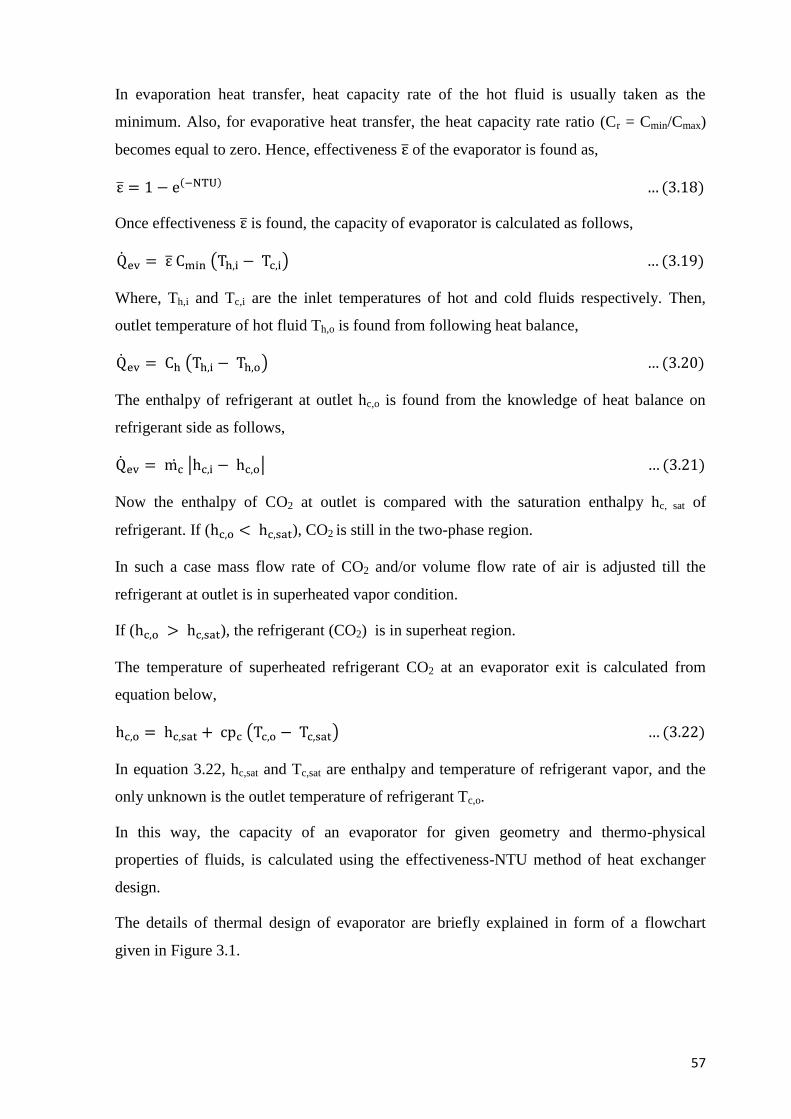
The details of thermal design of evaporator are briefly explained in form of a flowchart

given in Figure 3.1.

58

Figure 3.1: Flowchart for thermal design of an evaporator

3.2.2 Flow patterns during co2 evaporation

Flow patterns are very important in understanding the very complex two-phase flow

phenomena and heat transfer trends in flow boiling. To predict the local flow patterns in a

channel, a flow pattern map is used. Cheng et al. [CRQT 08] has developed flow boiling

Is, 50 ≤ Ġc ≤ 1500 kg/s-m2?

Calculate: Ġh, Ġc,

Start

Read known geometry of evaporator: Do, δtube, Pt, Pl, Nt,r, Nt,c, Wc, δfin, Pfin

Calculate remainder geometry of the evaporator: Di, Nt, Hc, Lc, Lt, Nfin

Read upstream air parameters: Th,i, Ph,i, rhh,i, cph,i, ρh,i, μh,i, kh,i, Prh,i,

Calculate: Afr, At, and Amf on both fluid sides, and βHx of evaporator

Read refrigerant inlet parameters: Tc,i, Pc,i, xc,i, cpc,i, ρc,i, , hc,i, hc,sat

Calculate: Rcond, Rin, uh,f, uh,c, ReDo, RePl, jc, ,

ηfin, ηout, Rout, Rf,in, Rtotal, UA, NTU, ε, Th,o, Tc,o

Adjust

NO

Adjust

and/or

No

End

Is, 9 ≤ Tc,o ≤ 20 oC ?

Display Results

59

heat transfer model based on the Cheng–Ribatski–Wojtan–Thome CO2 flow pattern map

[CRWT 06]. This model accurately predicts changes of trends in flow boiling data, which

indicates the flow patterns such as onset of dry-out and onset of mist flow. In the present

study, the physical properties of CO2 have been obtained from built-in fluid property

function of EES. Based on the quality of CO2 at evaporator inlet (xc,i) and the mass flux

(Ġc), the flow patterns in the flow passage are first determined from the updated flow-

pattern map. In this model accurately accounted the transitions in flow patterns such as

annular flow to dryout (A–D), dryout to mist flow (D–M) and intermittent flow to bubbly

flow (I–B) transition curves.

The void fraction ‘ε’ and dimensionless geometrical parameters ALD, AVD, hLD and PiD used

in the flow pattern map are defined in the equations 3.23 to equation 3.27. Here, ALD is

dimensionless cross-sectional area occupied by liquid phase [-], AVD is dmensionless cross-

sectional area occupied by vapor phase [-], hLD is dimensionless vertical height of liquid

phase of refrigerant [-] and PiD is dimensionless perimeter of interface of vapour and liquid

phase.

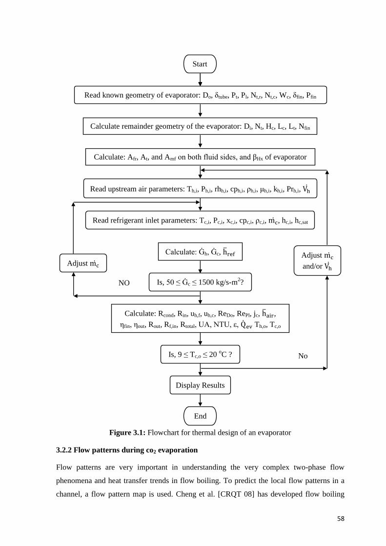
Where, the stratified angle, θstrat (which is the same as θdry of Figure 3.2) is calculated using

the equation (3.28) proposed by Biberg, [CRQT 08],

60

Figure 3.2: Stratified two-phase flow in a horizontal channel

The stratified-wavy to intermittent and annular flow (SW–I/A) transition boundary has been

calculated with the Kattan–Thome–Favrat criterion [CRQT 08] as,

Where, the liquid Froude number FrL and the liquid Weber number WeL are defined by

equation 3.30.

Then, the stratified-wavy flow region is subdivided into three zones according the criteria

by Wojtan et al. [CRQT 08],

Ġc > Ġwavy(xIA) gives the slug zone;

Ġstrat < Ġc < Ġwavy(xIA) and x < xIA give the slug/stratified-wavy zone;

x ≥ xIA gives the stratified-wavy zone.

The stratified to stratified-wavy flow (S–SW) transition boundary is calculated with the

Kattan–Thome–Favrat criterion [CRQT 08],

For the new flow pattern map: Ġstrat = Ġstrat(xIA) at x < xIA.

61

The intermittent to annular flow (I–A) transition boundary is calculated with the Cheng–

Ribatski–Wojtan–Thome criterion [CRWT 06] as,

Then, the transition boundary is extended down to its intersection with Ġstrat.

The annular flow to dryout region (A–D) transition boundary is calculated with the new

modified criterion of Wojtan et al. [CRQT 08] based on the dryout data of CO2 in this study

as,

Which, is extracted from the new dryout inception equation in the study as,

The vapor Weber number WeV, vapor Froude number FrV,Mori defined by Mori et al.

[MYOK 00], and the critical heat flux qcrit as per Kutateladze correlation [CRQT 08] are

calculated,

The dryout region to mist flow (D–M) transition boundary is calculated with the news

criterion developed by Cheng et al. [CRQT 08] based on the dryout completion data for

CO2 as,

62

Which, is extracted from the dryout completion equation developed by Cheng et al. [CRQT

08] for Ġmist calculation from,

The intermittent to bubbly flow (I–B) transition boundary is calculated with the criterion,

which arises at very high mass velocities and low qualities as shown in equation 3.41.

If Ġc > ĠB and x < xIA, then the flow is bubbly flow (B). The following conditions are

applied to the transitions in the high vapor quality range,

If Ġstrat(x) ≥ Ġdryout(x), then Ġdryout(x) = Ġstrat(x)

If Ġwavy(x) ≥ Ġdryout(x), then Ġdryout(x) = Ġwavy(x)

If Ġdryout(x) ≥ Ġmist(x), then Ġdryout(x) = Ġmist(x)

3.2.3 CO2 - side heat transfer coefficient

Once the flow patterns present along the flow path are identified, the local heat transfer

coefficients for respective flow patterns are calculated by the procedure outlined below. An

updated general flow boiling heat transfer model based on flow patterns developed by

Cheng et al. [CRT 08] has been used to calculate the local and average heat transfer

coefficients for evaporation heat transfer of CO2. The detailed procedure is given below.

The Kattan–Thome–Favrat general equation for the local flow boiling heat transfer

coefficients htp in a horizontal tube is used as the basic flow boiling expression which is as,

Where, θdry is the dry angle as shown in Figure 3.3 as follows,

63

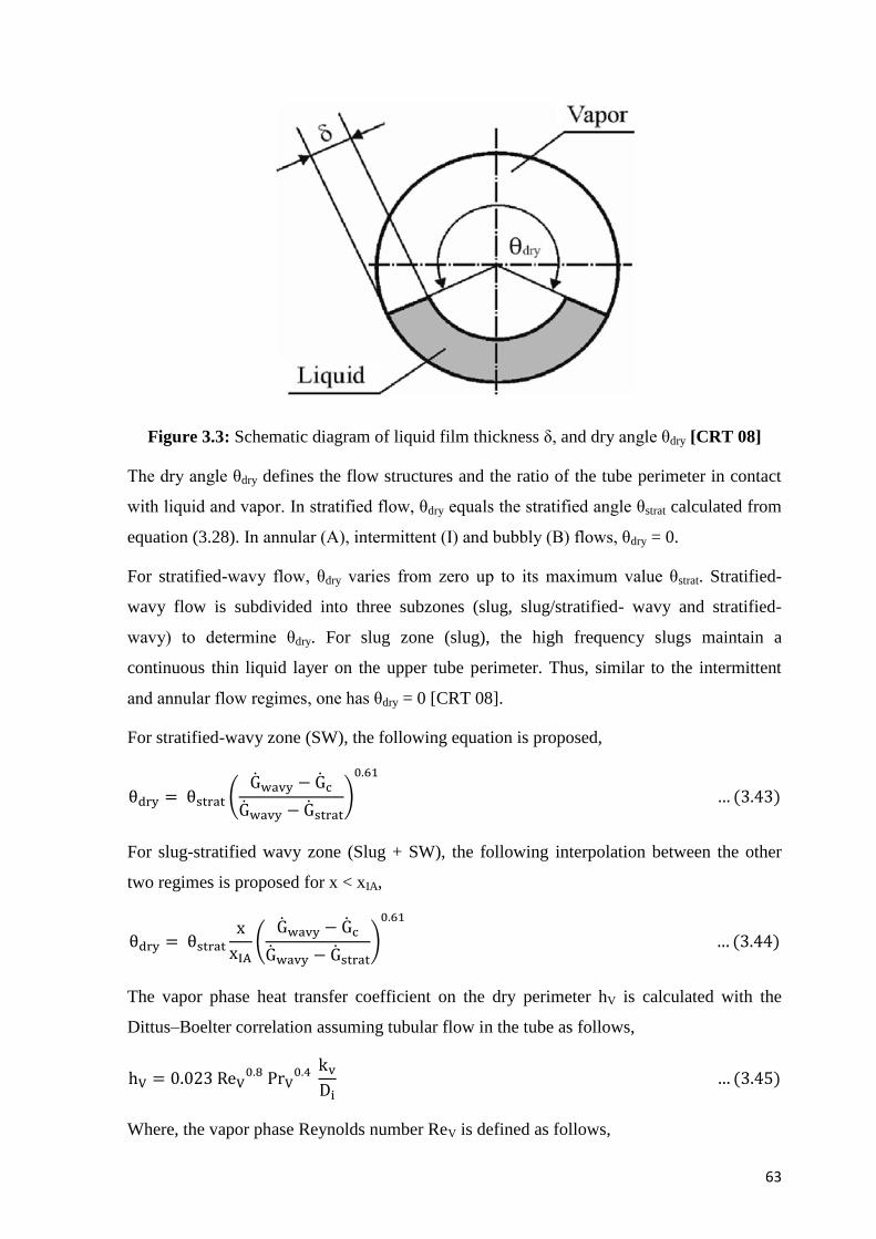
Figure 3.3: Schematic diagram of liquid film thickness δ, and dry angle θdry [CRT 08]

The dry angle θdry defines the flow structures and the ratio of the tube perimeter in contact

with liquid and vapor. In stratified flow, θdry equals the stratified angle θstrat calculated from

equation (3.28). In annular (A), intermittent (I) and bubbly (B) flows, θdry = 0.

For stratified-wavy flow, θdry varies from zero up to its maximum value θstrat. Stratified-

wavy flow is subdivided into three subzones (slug, slug/stratified- wavy and stratified-

wavy) to determine θdry. For slug zone (slug), the high frequency slugs maintain a

continuous thin liquid layer on the upper tube perimeter. Thus, similar to the intermittent

and annular flow regimes, one has θdry = 0 [CRT 08].

For stratified-wavy zone (SW), the following equation is proposed,

For slug-stratified wavy zone (Slug + SW), the following interpolation between the other

two regimes is proposed for x < xIA,

The vapor phase heat transfer coefficient on the dry perimeter hV is calculated with the

Dittus–Boelter correlation assuming tubular flow in the tube as follows,

Where, the vapor phase Reynolds number ReV is defined as follows,

64

The heat transfer coefficient on the wet perimeter hwet is calculated with an asymptotic

model that combines the nucleate boiling and convective boiling heat transfer contributions

to flow boiling heat transfer by the third power as follows,

Where, hnb, S and hcb are respectively nucleate boiling heat transfer coefficient, nucleate

boiling heat transfer suppression factor and convective boiling heat transfer coefficient and

are determined in the following equations.

The nucleate boiling heat transfer coefficient hnb is calculated with the Cheng–Ribatski–

Wojtan–Thome [CRWT 06] nucleate boiling correlation for CO2 which is a modification of

the Cooper correlation, as follows,

The Cheng–Ribatski–Wojtan–Thome [CRWT 06] nucleate boiling heat transfer suppression

factor S for CO2 is applied to reduce the nucleate boiling heat transfer contribution due to

the thinning of the annular liquid film.

Furthermore for non-circular channels, if Deq > 7.53 mm, then set Deq = 7.53 mm (use

instead of Di for non-circular channels in the equations). The liquid film

thickness ‘δ’ shown in Figure 3.3 is calculated with the expression proposed by El Hajal et

al. [CRT 08] as follows,

Where, the cross sectional area occupied by liquid phase of refrigerant, AL = A (1-ε), based

on the equivalent diameter (Di for circular channels) as shown in Figure 3.2. When the

liquid occupies more than one-half of the cross-section of the tube at low vapor quality,

equation 3.51 would yield a value of δ > Deq/2, which is not geometrically realistic.

65

Hence, whenever equation 3.51 gives δ > Deq/2, δ is set equal to Deq/2 (occurs when ε <

0.5). The liquid film δIA is calculated with equation 3.51 at the intermittent (I) to annular

flow (A) transition. (Note: Deq for non-circular channels, Di for circular channels)

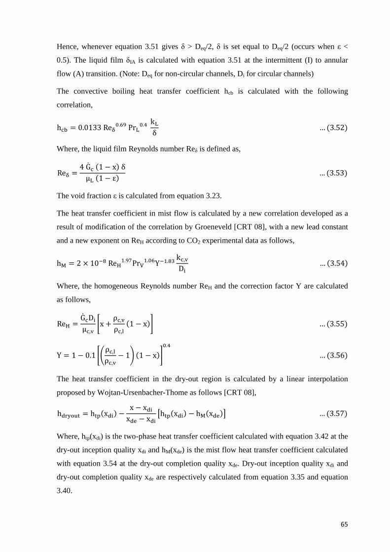
The convective boiling heat transfer coefficient hcb is calculated with the following

correlation,

Where, the liquid film Reynolds number Reδ is defined as,

The void fraction ε is calculated from equation 3.23.

The heat transfer coefficient in mist flow is calculated by a new correlation developed as a

result of modification of the correlation by Groeneveld [CRT 08], with a new lead constant

and a new exponent on ReH according to CO2 experimental data as follows,

Where, the homogeneous Reynolds number ReH and the correction factor Y are calculated

as follows,

The heat transfer coefficient in the dry-out region is calculated by a linear interpolation

proposed by Wojtan-Ursenbacher-Thome as follows [CRT 08],

Where, htp(xdi) is the two-phase heat transfer coefficient calculated with equation 3.42 at the

dry-out inception quality xdi and hM(xde) is the mist flow heat transfer coefficient calculated

with equation 3.54 at the dry-out completion quality xde. Dry-out inception quality xdi and

dry-out completion quality xde are respectively calculated from equation 3.35 and equation

3.40.

66

The vapor Weber number Wev and the vapor Froude number FrV,Mori defined by Mori et al.

[MYOK 00] are calculated from equation 3.36 and equation 3.37, and the critical heat flux

qcrit is calculated with the Kutateladze correlation from equation 3.38. If xde is not defined at

the mass velocity being considered, it is assumed that xde = 0.999.

A heat transfer model for bubbly flow was added by Cheng et al. [CRT 08] to the model for

the sake of completeness. In absence of any data, the heat transfer coefficients in bubbly

flow regime are calculated by the same method as that in the intermittent flow.

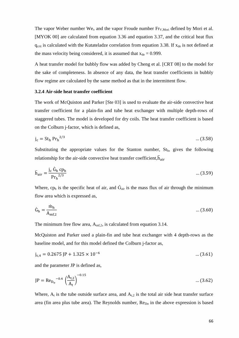
3.2.4 Air-side heat transfer coefficient

The work of McQuiston and Parker [Ste 03] is used to evaluate the air-side convective heat

transfer coefficient for a plain-fin and tube heat exchanger with multiple depth-rows of

staggered tubes. The model is developed for dry coils. The heat transfer coefficient is based

on the Colburn j-factor, which is defined as,

Substituting the appropriate values for the Stanton number, Sth, gives the following

relationship for the air-side convective heat transfer coefficient,

Where, cph is the specific heat of air, and Ġair is the mass flux of air through the minimum

flow area which is expressed as,

The minimum free flow area, Amf,2, is calculated from equation 3.14.

McQuiston and Parker used a plain-fin and tube heat exchanger with 4 depth-rows as the

baseline model, and for this model defined the Colburn j-factor as,

and the parameter JP is defined as,

Where, At is the tube outside surface area, and At,2 is the total air side heat transfer surface

area (fin area plus tube area). The Reynolds number, ReDo in the above expression is based

67

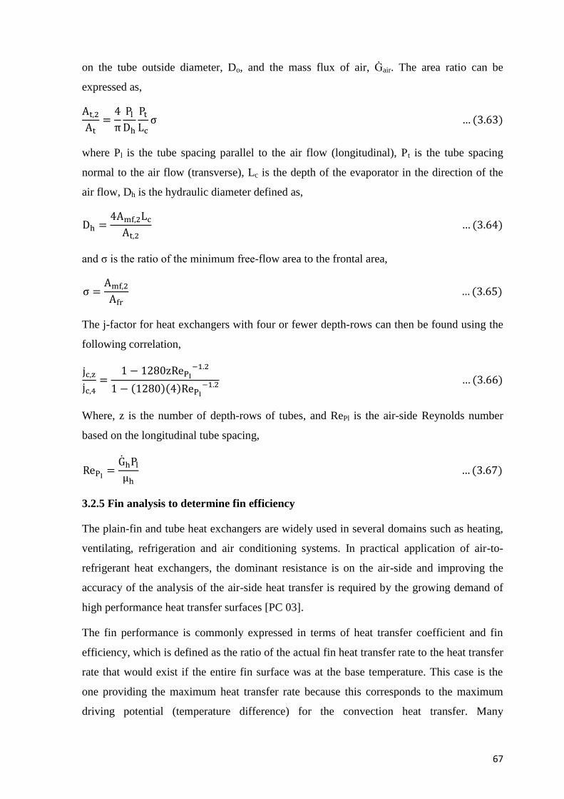
on the tube outside diameter, Do, and the mass flux of air, Ġair. The area ratio can be

expressed as,

where Pl is the tube spacing parallel to the air flow (longitudinal), Pt is the tube spacing

normal to the air flow (transverse), Lc is the depth of the evaporator in the direction of the

air flow, Dh is the hydraulic diameter defined as,

and ζ is the ratio of the minimum free-flow area to the frontal area,

The j-factor for heat exchangers with four or fewer depth-rows can then be found using the

following correlation,

Where, z is the number of depth-rows of tubes, and RePl is the air-side Reynolds number

based on the longitudinal tube spacing,

3.2.5 Fin analysis to determine fin efficiency

The plain-fin and tube heat exchangers are widely used in several domains such as heating,

ventilating, refrigeration and air conditioning systems. In practical application of air-to-

refrigerant heat exchangers, the dominant resistance is on the air-side and improving the

accuracy of the analysis of the air-side heat transfer is required by the growing demand of

high performance heat transfer surfaces [PC 03].

The fin performance is commonly expressed in terms of heat transfer coefficient and fin

efficiency, which is defined as the ratio of the actual fin heat transfer rate to the heat transfer

rate that would exist if the entire fin surface was at the base temperature. This case is the

one providing the maximum heat transfer rate because this corresponds to the maximum

driving potential (temperature difference) for the convection heat transfer. Many

68

experimental studies are available in the open literature to characterize the air-side heat

transfer performance for several types of fins used in finned tube heat exchangers. The

established correlations are used for design, rating and modeling of heat exchangers. What

is observed in nearly all published papers is that, whatever the fin type (plain, louvered,

slit), the fin efficiency calculation is always performed by analytical methods derived from

circular fin analysis [PC03].

The analytical circular fin analysis involves a number of assumptions, known as ideal fin

assumptions, which need to be addressed. These assumptions are:

one-dimensional radial conduction,

steady state conditions,

radiation heat transfer negligible,

constant fin conductivity,

constant heat transfer coefficient over the entire fin,

fin base temperature is assumed to be constant,

thermal contact resistance between the prime surface and the fin is negligible,

the surrounding fluid is assumed at constant temperature.

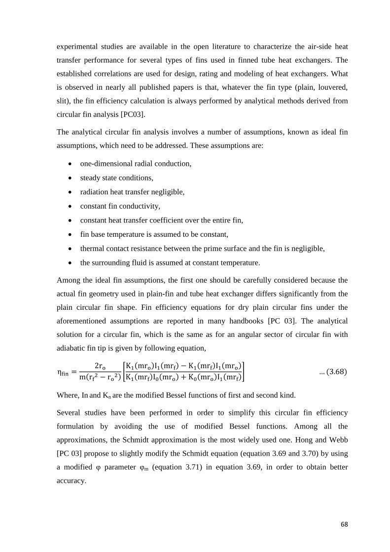
Among the ideal fin assumptions, the first one should be carefully considered because the

actual fin geometry used in plain-fin and tube heat exchanger differs significantly from the

plain circular fin shape. Fin efficiency equations for dry plain circular fins under the

aforementioned assumptions are reported in many handbooks [PC 03]. The analytical

solution for a circular fin, which is the same as for an angular sector of circular fin with

adiabatic fin tip is given by following equation,

Where, In and Kn are the modified Bessel functions of first and second kind.

Several studies have been performed in order to simplify this circular fin efficiency

formulation by avoiding the use of modified Bessel functions. Among all the

approximations, the Schmidt approximation is the most widely used one. Hong and Webb

[PC 03] propose to slightly modify the Schmidt equation (equation 3.69 and 3.70) by using

a modified φ parameter φm (equation 3.71) in equation 3.69, in order to obtain better

accuracy.

69

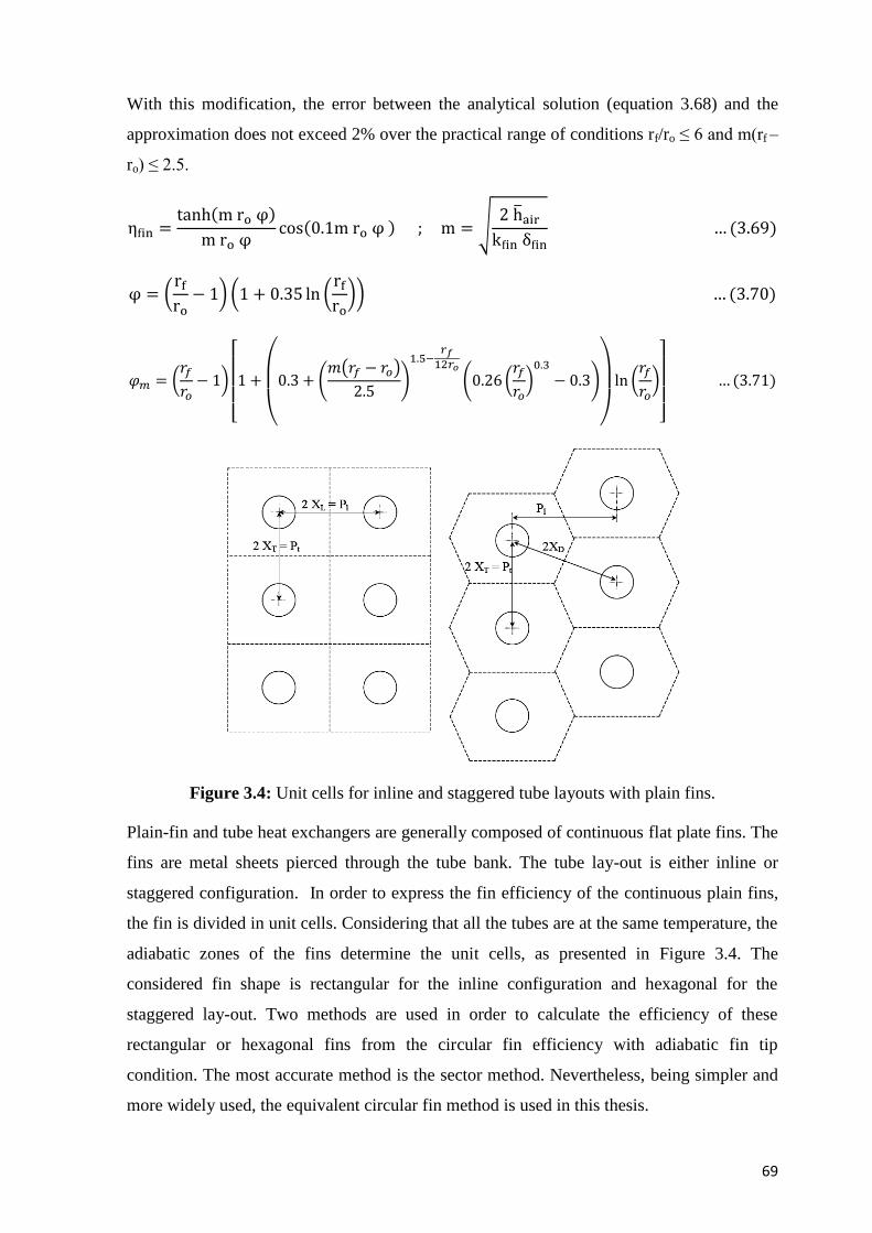
With this modification, the error between the analytical solution (equation 3.68) and the

approximation does not exceed 2% over the practical range of conditions rf/ro ≤ 6 and m(rf –

ro) ≤ 2.5.

Figure 3.4: Unit cells for inline and staggered tube layouts with plain fins.

Plain-fin and tube heat exchangers are generally composed of continuous flat plate fins. The

fins are metal sheets pierced through the tube bank. The tube lay-out is either inline or

staggered configuration. In order to express the fin efficiency of the continuous plain fins,

the fin is divided in unit cells. Considering that all the tubes are at the same temperature, the

adiabatic zones of the fins determine the unit cells, as presented in Figure 3.4. The

considered fin shape is rectangular for the inline configuration and hexagonal for the

staggered lay-out. Two methods are used in order to calculate the efficiency of these

rectangular or hexagonal fins from the circular fin efficiency with adiabatic fin tip

condition. The most accurate method is the sector method. Nevertheless, being simpler and

more widely used, the equivalent circular fin method is used in this thesis.

70

Gardner and Schmidt [PC 03], in their respective studies, have shown that in the case of

rectangular and hexagonal fins, the fin efficiency could be treated as a circular fin, by

considering an equivalent circular fin radius. For the calculation of the equivalent circular

radius, two approaches are possible. The first one consists in considering a circular fin

having the same surface area as the rectangular or hexagonal fin. The other method is the

Schmidt method in which correlations are developed in order to find an equivalent circular

fin having the same fin efficiency as the rectangular fin (equation 3.72) or the hexagonal fin

(equation 3.73).

Equations 3.69), equation 3.71, and equation 3.73 are used to calculate the fin efficiency of

plain-fins for staggered tube layout.

3.2.6 CO2 - side two-phase pressure drop

A new two-phase frictional pressure drop model for CO2 is developed by Cheng et al.

[CRQT 08] This model has incorporated the updated CO2 flow pattern map, which is used

to calculate two-phase pressure drop during evaporation of CO2. This is a phenomenological

two-phase frictional pressure drop model, which is intrinsically related to the flow patterns.

Based on quality and mass flux of CO2 refrigerant at the evaporator inlet, first the two-phase

flow patterns possible along the flow path are decided as aforementioned in section 3.7. The

total pressure drop is the sum of the static pressure drop (gravity pressure drop), the

momentum pressure drop (acceleration pressure drop) and the frictional pressure drop,

For horizontal channels, the static pressure drop equals zero. The momentum pressure drop

is calculated as,

71

CO2 frictional pressure drop model for annular flow (A) [CRQT 08]: The basic equation is

the same as that of the Moreno Quibén and Thome pressure drop model as,

Where, the two-phase flow friction factor of annular flow fA is calculated by equation 3.77.

This correlation is thus different from that of the Moreno Quibén and Thome pressure drop

model. The mean velocity of the vapor phase uc,v is calculated by equation 3.78.

The void fraction ‘ε’ is calculated using equation 3.23. The vapor phase Reynolds number

ReV and the liquid phase Weber number WeL are based on the mean liquid phase velocity

uc,l .

CO2 frictional pressure drop model for slug and intermittent flow (Slug + I) [CRQT 08]

To avoid jump in the pressure drops between these two flow patterns, the Moreno Quibén

and Thome pressure drop model is updated as given in equation 3.82.

Where, ΔpA is calculated with equation 3.76 and the single-phase frictional pressure drop

considering the total vapor–liquid two-phase flow as liquid flow ΔpLO is calculated by

equation 3.83.

72

The friction factor is calculated with the Blasius equation as,

Where, Reynolds number ReLO is calculated as,

CO2 frictional pressure drop model for stratified-wavy flow (SW) [CRQT 08]: The equation

is kept the same as that of the Moreno Quibén and Thome pressure drop model as,

Where, the two-phase friction factor of stratified-wavy flow fSW is calculated with the

following interpolating expression (a modification of that used in the Moreno Quibén and

Thome pressure drop model) based on the CO2 database as,

and the dimensionless dry angle θ*dry is defined as,

For θdry in the stratified-wavy regime (SW), the following equation is proposed,

The single-phase friction factor of the vapor phase fV is calculated as,

Where, the vapor Reynolds number is calculated with equation (3.79).

CO2 frictional pressure drop model for slug-stratified wavy flow (Slug + SW) [CRQT 08]:

The authors propose to avoid any jump in the pressure drops between these two flow

patterns and to updated the Moreno Quibén and Thome pressure drop model as,

73

Where, ΔpLO and ΔpSW are calculated with equation 3.83 and 3.86 respectively.

CO2 frictional pressure drop model for mist flow (M) [CRQT 08]:

The following expression is kept the same as that in the Moreno Quibén and Thome

pressure drop model as,

The homogenous density ρc,h is defined as,

Where, the homogenous void fraction εh is calculated as,

And the friction factor of mist flow fM was correlated according to the CO2 experimental

data, which is different from that in the Moreno Quibén and Thome pressure drop model by

equation 3.95.

The mist flow Reynolds number is defined as,

Where, the homogenous dynamic viscosity is calculated as proposed by Cicchitti et al.

[CLSS 60] in equation 3.97.

The constants in equation (3.95) are quite different from those in the Blasius equation.

According to Cheng et al. [CRQT 08], the reason is possibly because there are limited

experimental data in mist flow in the database and also perhaps a lower accuracy of these

experimental data. Therefore, Cheng et al. [CRQT 08] feel the need for more accurate

74

experimental data in mist flow to further verify this correlation or modify it if necessary in

the future.

CO2 frictional pressure drop model for dryout region (D) [CRQT 08]:

The linear interpolating expression is kept the same as that in the Moreno Quibén–Thome

pressure drop model as,

Where, Δptp(xdi) is the frictional pressure drop at the dryout inception quality xdi and is

calculated with equation 3.76 for annular flow or with equation 3.86 for stratified-wavy

flow, and ΔpM(xde) is the frictional pressure drop at the dryout completion quality xde and is

calculated with equation 3.92. xdi and xde are calculated with equations 3.35 and 3.40

respectively.

CO2 frictional pressure drop model for stratified flow (S) [CRQT 08]:

The Cheng et al. [CRQT 08] found that no data fell into this flow regime but for

completeness, they kept the method the same as that in the Moreno Quibén and Thome

pressure drop model as,

Where, the mean velocity of the vapor phase uc,v is calculated with equation 3.78 and the

two-phase friction factor of stratified flow is calculated as,

The single-phase friction factor of the vapor phase fV and the two-phase friction factor of

annular flow fA are calculated with equation 3.90 and equation 3.77 respectively, and the

dimensionless stratified angle θ*strat is defined as,

Where, the stratified angle θstrat is calculated with equation 3.28.

Where, ΔpLO and are calculated with equation 3.83 and 3.99 respectively.

75

CO2 frictional pressure drop model for bubbly flow (B) [CRQT 08]: In their study, the

authors found no data available for this regime but keeping consistency with the frictional

pressure drops in the neighboring regimes and following the same format as the others

without creating a jump at the transition (there is no such a model in the Moreno Quibén

and Thome pressure drop model), the following expression is proposed as,

Where, ΔpLO and ΔpA are calculated with equation 3.83 and 3.76 respectively.

According to Cheng et al. [CRQT 08], further experimental data are needed to verify or

modify this model for bubbly flow regime.

3.2.7 Air-side pressure drop

According to Rich, the air-side pressure drop can be divided into two components, the

pressure drop due to the tubes, Δptubes, and the pressure drop due to the fins, Δpfin. The work

of Rich [Wri 00] is used to evaluate the air-side pressure drop due to the fins, which is

expressed as,

where, ffins is the fin friction factor, vm is the mean specific volume of air, Ġh is mass flux of

air, As is the finned (secondary) surface area, and Amf,2 is the air-side minimum free flow

area. In experimental tests, Rich found that the friction factor is dependent on the Reynolds

number, but it is independent of the fin spacing for fin density between 3 and 14 fins per

inch. In this range of fin density, Rich expresses the fin friction factor as,

Where, the Reynolds number RePl is based on the tube longitudinal spacing, Pl,

To determine the pressure drop over the tubes, the relationships developed by Kim-Youn-

Webb [Jia 03] are used. The tube-side friction factor and pressure drop is expressed as,

76

where, Pt is tube transverse pitch, Do is tube outside diameter, At,o is tube outside surface

area, and ReDo is air-side Reynolds number based on tube outside diameter found as,

3.2.8 Modification in IMST ART for evaporator

The geometry of an evaporator finalized using Engineering Equation Solver (EES) [Kli 10]

is further modified in IMST ART [CGMB 02]. The geometry and performance parameters

of individual components have an effect on the system energy performance. In case of an

evaporator, the parameters like air side pressure drop, refrigerant pressure drop, refrigerant

flow circuits, tube longitudinal and lateral pitch, overall refrigerant charge, refrigerant side

pressure drop etc. have effect on the system overall performance parameters. The geometry

of an evaporator is further fine tuned through the parametric simulation study to achieve

maximum energy performance of the system for the rated conditions.

3.3 SUCTION LINE HEAT EXHANGER (SLHX)

A SLHX is used to transfer heat from supercritical high pressure and temperature CO2 to

subcritical low pressure and low temperature CO2. The transfer of heat results in the cooling

of the supercritical gas or liquid and heating of the subcritical CO2 vapor. This transfer of

the heat has impact on the performance of the transcritical CO2 cycle. The literature review

has shown that a SLHX in the cycle increases the Coefficient of Performance (COP) of the

cycle in the range 5% to 10%.

This part focuses on developing the mathematical iterative method to predict the heat

transfer coefficient as well as pressure drop for a straight tube in tube type heat exchanger.

Further, the CFD model to predict the heat transfer as well as pressure drop between the

subcritical and supercritical CO2 in a straight tube in tube type heat exchanger has been

discussed.

77

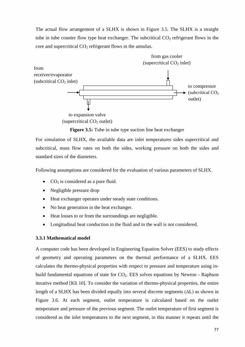
The actual flow arrangement of a SLHX is shown in Figure 3.5. The SLHX is a straight

tube in tube counter flow type heat exchanger. The subcritical CO2 refrigerant flows in the

core and supercritical CO2 refrigerant flows in the annulus.

Figure 3.5: Tube in tube type suction line heat exchanger

For simulation of SLHX, the available data are inlet temperatures sides supercritical and

subcritical, mass flow rates on both the sides, working pressure on both the sides and

standard sizes of the diameters.

Following assumptions are considered for the evaluation of various parameters of SLHX.

CO2 is considered as a pure fluid.

Negligible pressure drop

Heat exchanger operates under steady state conditions.

No heat generation in the heat exchanger.

Heat losses to or from the surroundings are negligible.

Longitudinal heat conduction in the fluid and in the wall is not considered.

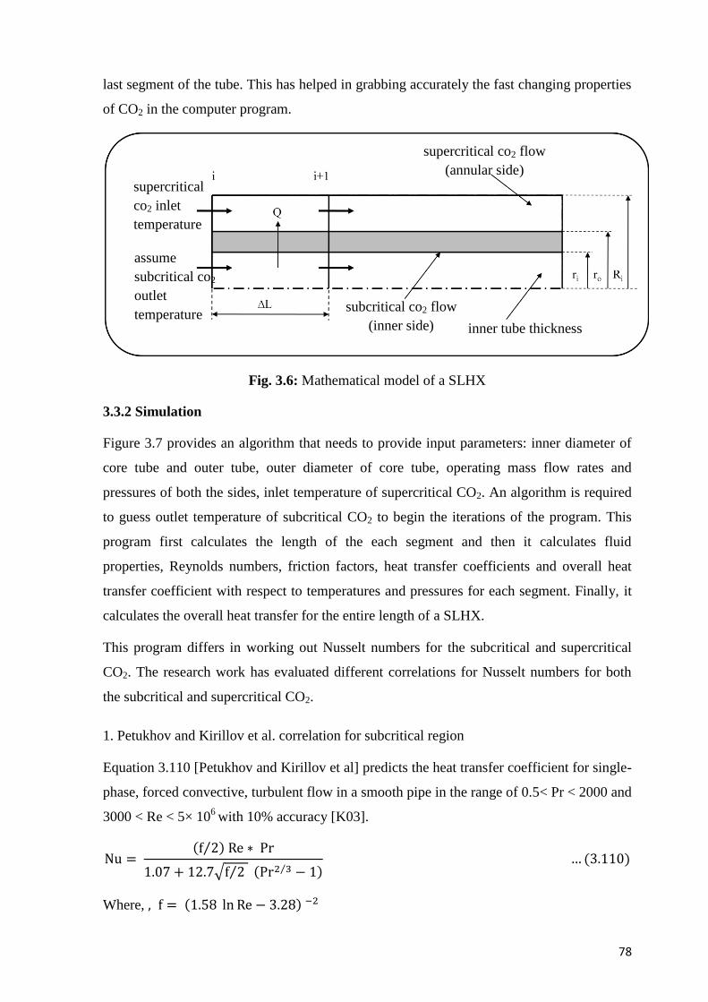
3.3.1 Mathematical model

A computer code has been developed in Engineering Equation Solver (EES) to study effects

of geometry and operating parameters on the thermal performance of a SLHX. EES

calculates the thermo-physical properties with respect to pressure and temperature using in-

build fundamental equations of state for CO2. EES solves equations by Newton - Raphson

iterative method [Kli 10]. To consider the variation of thermo-physical properties, the entire

length of a SLHX has been divided equally into several discrete segments (∆L) as shown in

Figure 3.6. At each segment, outlet temperature is calculated based on the outlet

temperature and pressure of the previous segment. The outlet temperature of first segment is

considered as the inlet temperatures to the next segment, in this manner it repeats until the

to expansion valve

(supercritical CO2 outlet)

to compressor

(subcritical CO2

outlet)

from gas cooler

(supercritical CO2 inlet) from

receiver/evaporator

(subcritical CO2 inlet)

78

last segment of the tube. This has helped in grabbing accurately the fast changing properties

of CO2 in the computer program.

Fig. 3.6: Mathematical model of a SLHX

3.3.2 Simulation

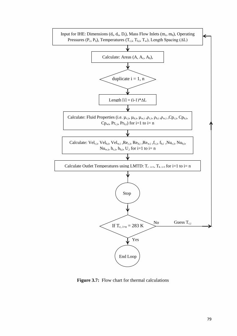
Figure 3.7 provides an algorithm that needs to provide input parameters: inner diameter of

core tube and outer tube, outer diameter of core tube, operating mass flow rates and

pressures of both the sides, inlet temperature of supercritical CO2. An algorithm is required

to guess outlet temperature of subcritical CO2 to begin the iterations of the program. This

program first calculates the length of the each segment and then it calculates fluid

properties, Reynolds numbers, friction factors, heat transfer coefficients and overall heat

transfer coefficient with respect to temperatures and pressures for each segment. Finally, it

calculates the overall heat transfer for the entire length of a SLHX.

This program differs in working out Nusselt numbers for the subcritical and supercritical

CO2. The research work has evaluated different correlations for Nusselt numbers for both

the subcritical and supercritical CO2.

1. Petukhov and Kirillov et al. correlation for subcritical region

Equation 3.110 [Petukhov and Kirillov et al] predicts the heat transfer coefficient for single-

phase, forced convective, turbulent flow in a smooth pipe in the range of 0.5< Pr < 2000 and

3000 < Re < 5× 106

with 10% accuracy [K03].

Where,

supercritical

co2 inlet

temperature

assume

subcritical co2

outlet

temperature

supercritical co2 flow

(annular side)

subcritical co2 flow

(inner side)

inner tube thickness

79

Figure 3.7: Flow chart for thermal calculations

Input for IHE: Dimensions (di, do, Di), Mass Flow Inlets (mc, mh), Operating

Pressures (Pc, Ph), Temperatures (Tc,i, Th,i, Tw), Length Spacing (∆L)

Calculate: Areas (A, Ac, Ah),

Calculate: Fluid Properties (i.e. µc,i, µh,i, µw,i ,ρc,i, ρh,i ,ρw,i ,Cpc,i, Cph,i,

Cpwi, Prc,i, Prh,i) for i=1 to i= n

Calculate: Velc,i, Velh,i, Velw,i ,Rec,i, Reh,i ,Rew,i ,fc,i, fh,i ,Nuc,i, Nuh,i,

Nuw,i, hc,i, hh,i, U,i for i=1 to i= n

Calculate Outlet Temperatures using LMTD: Tc, i+1, Th, i+1 for i=1 to i= n

No

Yes

Guess Tc,i

Length [i] = (i-1)*∆L

Stop

End Loop

If Tc, i+n = 283 K

duplicate i = 1, n

80

2. Pitla et al. correlation for supercritical region

The correlation of Pitla et al. [PGR 01] has been used to predict the heat transfer coefficient

of supercritical CO2 during in-tube cooling. The correlation is given in Equation 3.111.

Where, Gnielinski correlation is used to calculate both Nusselt numbers Nuwall and Nubulk.

Here, subscripts ‘wall’ and ‘bulk’ represent that properties are evaluated at wall temperature

and bulk flow temperature respectively.

Where,

3. Chang et al. correlation for supercritical region

The correlation of Chang et al. [SP 05] has been used to evaluate the heat transfer

coefficient and pressure drop during gas cooling process of CO2 in supercritical region. The

authors have provided the separated correlations for region above and below the pseudo-

critical temperature (Tb/Tpc >1 and Tb/Tpc ≤ 1) on the thermodynamic property chart for

CO2.

The predicted heat transfer coefficient by new proposed correlation is within the accuracy of

10% with the experiment data.

The outlet temperatures of each segment are calculated by equating LMTD and energy

balance equations as shown by equations 3.114 and 3.115 respectively.

The outlet temperatures of first segment are considered as inlet temperature to the next

segment. In this manner, calculation repeats until the nth

segment and finally at segment i =

n, the gives the outlet temperature of the supercritical CO2 and inlet temperature of the

subcritical CO2. If temperature of the subcritical CO2 at i = n is equal to the guess

81

temperature of the subcritical CO2, then solution stops else need to adjust the guess value of

the outlet temperature of the subcritical CO2 at i = 1.

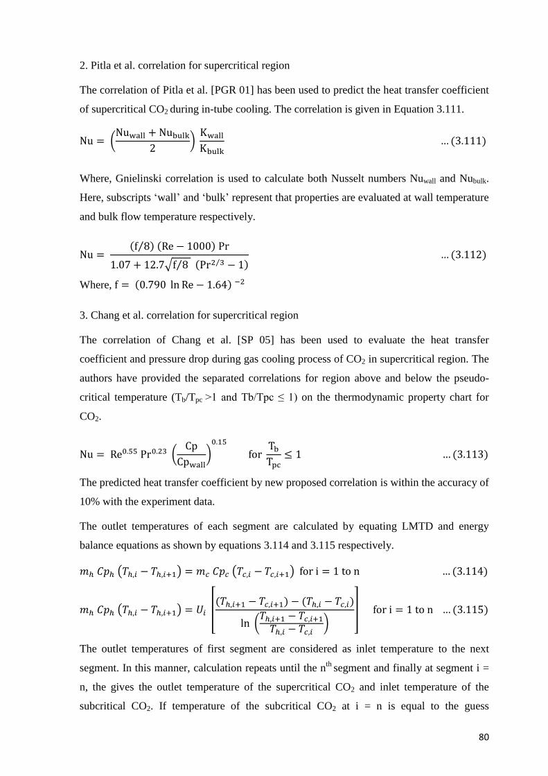
Figure 3.8: Flow chart for the pressure drop calculations

3.3.3 Pressure drop in a SLHX

An algorithm shown in Figure 3.8 provides the basic structure of the program to calculate

Reynold number and friction factor at bulk temperatures on the entire length of a SLHX.

This program uses Filonenko friction factor correlation for subcritical region and Petrov -

Popov friction factor correlation for supercritical region.

1. Filonenko's friction factor for subcritical region

Filonenko friction factor correlation 3.116 is widely used for the turbulent gas flow in

smooth tubes.

2. Petrov and Popov friction factor for supercritical region

Calculate: Heat Transfer & cross

sections Areas (A, Ac, Ah),

Calculate: Fluid & Solid Properties

Calculate: Velc, Velh, Velw, Rec, Reh, Rew, c, h

Calculate Pressure Drop ( )

Inputs: Dimensions (di, do, Di), Mass Flow Inlets (mc, mh), Operating Pressures

(Pc, Ph), Inlet, Outlet & wall Temperatures (Tc,i, Tc,o, Th,i, Th,o, Tw), Length (L)

Stop

82

Petrov and Popov calculated the friction factor of CO2 cooled in the supercritical conditions

in the range of Rewall = 1.4×104 -7.9×10

5 and Rebulk = 3.1×10

4- 8×10

5. Petrov and Popov

obtained an interpolation equation 3.117 of the friction factor.

ρ

ρ

Where fw, the friction factor is calculated by Filonenko Eqution 3.116 [Fil 48] at tube wall

temperature and the exponent ‘s’ is given by,

… (3.118)

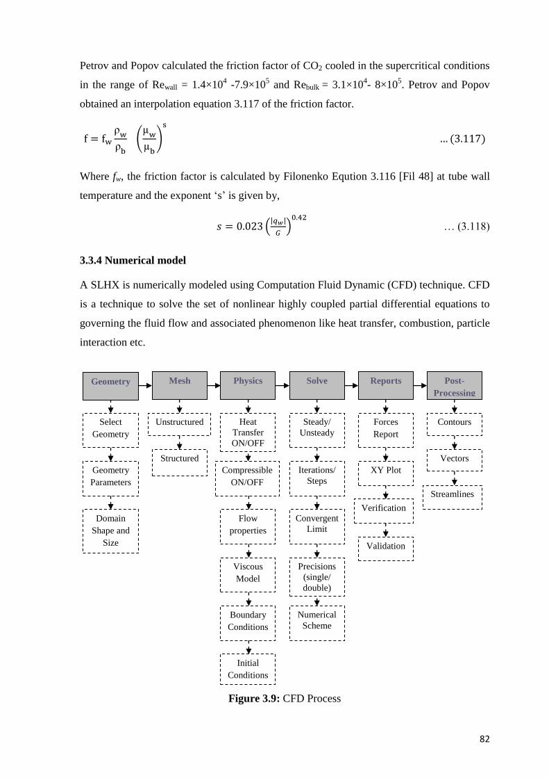
3.3.4 Numerical model

A SLHX is numerically modeled using Computation Fluid Dynamic (CFD) technique. CFD

is a technique to solve the set of nonlinear highly coupled partial differential equations to

governing the fluid flow and associated phenomenon like heat transfer, combustion, particle

interaction etc.

Figure 3.9: CFD Process

Viscous

Model

Boundary

Conditions

Initial

Conditions

Convergent

Limit

Contours

Precisions

(single/

double)

Numerical

Scheme

Vectors

Streamlines

Verification

Geometry

Select

Geometry

Geometry

Parameters

Physics Mesh Solve Post-

Processing

Compressible

ON/OFF

Flow

properties

Unstructured Steady/

Unsteady Forces

Report

XY Plot

Domain

Shape and

Size

Heat

Transfer

ON/OFF Structured

Iterations/

Steps

Validation

Reports

83

Figure 3.9 shows in detail the process of CFD. First the geometry has to be created with the

consideration of some CFD modeling constraints. This geometry then needs to be meshed.

Meshing or grid generation is a process in which the domain of interest is discretized in the

finite volumes. Appropriate models, such as the k – turbulence models, boundary

conditions and solver parameters are assigned as per the analysis requirements. Solver

solves the various governing equations iteratively to attain the defined convergence criteria.

The continuity, energy and momentum balance equations basically solved using CFD

algorithm.

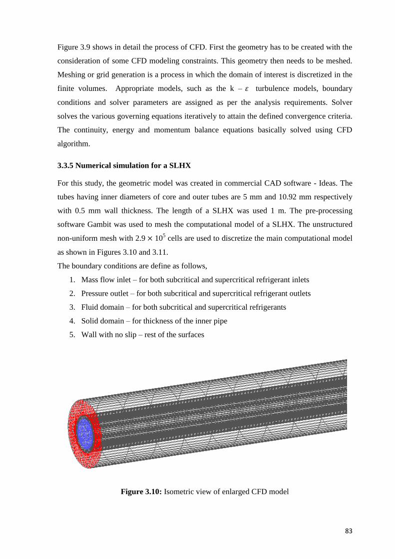
3.3.5 Numerical simulation for a SLHX

For this study, the geometric model was created in commercial CAD software - Ideas. The

tubes having inner diameters of core and outer tubes are 5 mm and 10.92 mm respectively

with 0.5 mm wall thickness. The length of a SLHX was used 1 m. The pre-processing

software Gambit was used to mesh the computational model of a SLHX. The unstructured

non-uniform mesh with 2.9 105 cells are used to discretize the main computational model

as shown in Figures 3.10 and 3.11.

The boundary conditions are define as follows,

1. Mass flow inlet – for both subcritical and supercritical refrigerant inlets

2. Pressure outlet – for both subcritical and supercritical refrigerant outlets

3. Fluid domain – for both subcritical and supercritical refrigerants

4. Solid domain – for thickness of the inner pipe

5. Wall with no slip – rest of the surfaces

Figure 3.10: Isometric view of enlarged CFD model

84

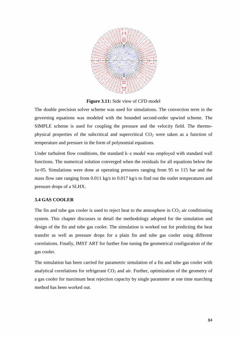
Figure 3.11: Side view of CFD model

The double precision solver scheme was used for simulations. The convection term in the

governing equations was modeled with the bounded second-order upwind scheme. The

SIMPLE scheme is used for coupling the pressure and the velocity field. The thermo-

physical properties of the subcritical and supercritical CO2 were taken as a function of

temperature and pressure in the form of polynomial equations.

Under turbulent flow conditions, the standard k–ε model was employed with standard wall

functions. The numerical solution converged when the residuals for all equations below the

1e-05. Simulations were done at operating pressures ranging from 95 to 115 bar and the

mass flow rate ranging from 0.011 kg/s to 0.017 kg/s to find out the outlet temperatures and

pressure drops of a SLHX.

3.4 GAS COOLER

The fin and tube gas cooler is used to reject heat to the atmosphere in CO2 air conditioning

system. This chapter discusses in detail the methodology adopted for the simulation and

design of the fin and tube gas cooler. The simulation is worked out for predicting the heat

transfer as well as pressure drops for a plain fin and tube gas cooler using different

correlations. Finally, IMST ART for further fine tuning the geometrical configuration of the

gas cooler.

The simulation has been carried for parametric simulation of a fin and tube gas cooler with

analytical correlations for refrigerant CO2 and air. Further, optimization of the geometry of

a gas cooler for maximum heat rejection capacity by single parameter at one time marching

method has been worked out.

85

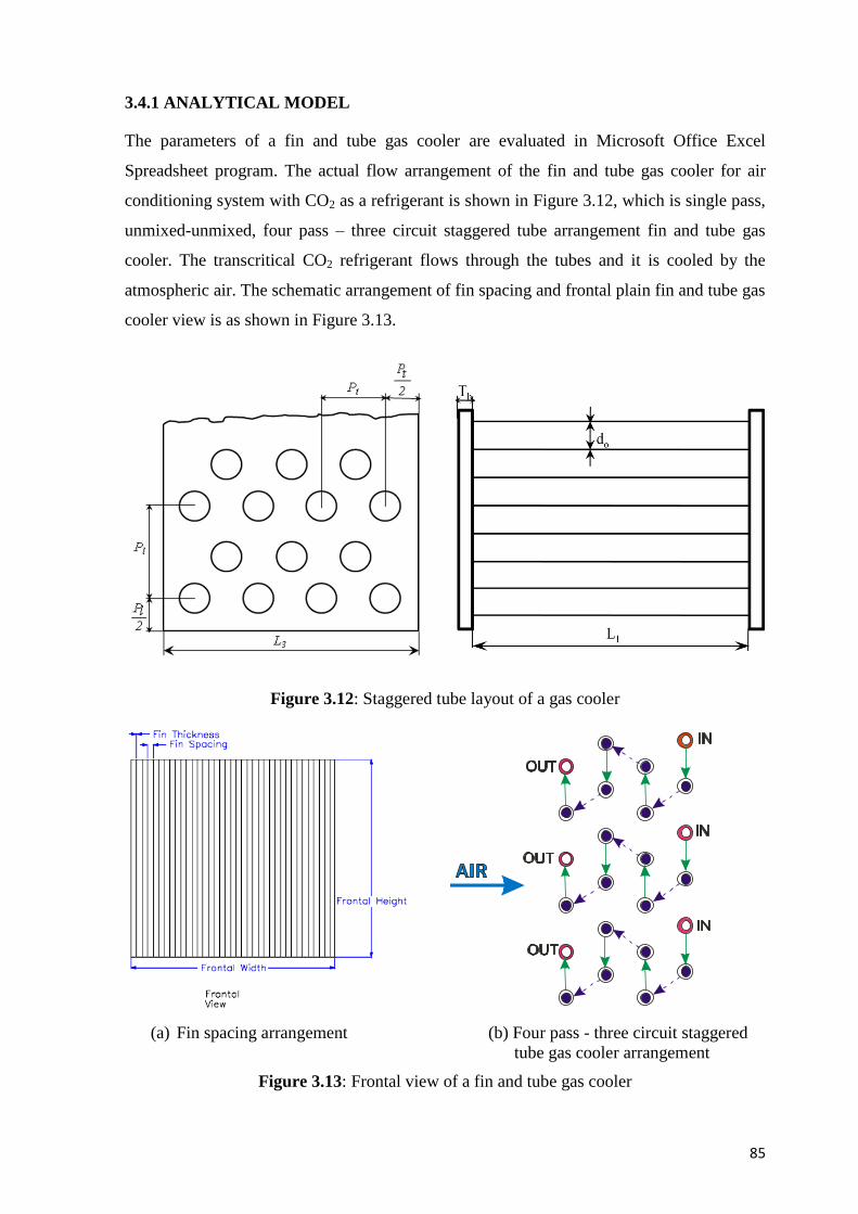
3.4.1 ANALYTICAL MODEL

The parameters of a fin and tube gas cooler are evaluated in Microsoft Office Excel

Spreadsheet program. The actual flow arrangement of the fin and tube gas cooler for air

conditioning system with CO2 as a refrigerant is shown in Figure 3.12, which is single pass,

unmixed-unmixed, four pass – three circuit staggered tube arrangement fin and tube gas

cooler. The transcritical CO2 refrigerant flows through the tubes and it is cooled by the

atmospheric air. The schematic arrangement of fin spacing and frontal plain fin and tube gas

cooler view is as shown in Figure 3.13.

Figure 3.12: Staggered tube layout of a gas cooler

(a) Fin spacing arrangement (b) Four pass - three circuit staggered

tube gas cooler arrangement

Figure 3.13: Frontal view of a fin and tube gas cooler

86

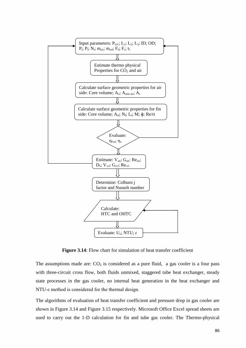
Figure 3.14: Flow chart for simulation of heat transfer coefficient

The assumptions made are: CO2 is considered as a pure fluid, a gas cooler is a four pass

with three-circuit cross flow, both fluids unmixed, staggered tube heat exchanger, steady

state processes in the gas cooler, no internal heat generation in the heat exchanger and

NTU-ε method is considered for the thermal design.

The algorithms of evaluation of heat transfer coefficient and pressure drop in gas cooler are

shown in Figure 3.14 and Figure 3.15 respectively. Microsoft Office Excel spread sheets are

used to carry out the 1-D calculation for fin and tube gas cooler. The Thermo-physical

Input parameters: PGC; L1; L2; L3; ID; OD;

Pt; Pl; Nt; mair; mref; Fd; Fs; tf

Estimate thermo physical

Properties for CO2 and air

Calculate surface geometric properties for air

side: Core volume; Ao; Amin air; At

Calculate surface geometric properties for fin

side: Core volume; Asf; Nf; Lf; M; ɸ; Re/rt

Evaluate:

ηFin; ηo

Estimate: Vair; Gair: Reair;

Dh; Vref; Gref; Reref

Determine: Colburn j

factor and Nusselt number

Calculate:

HTC and OHTC

Evaluate: Uo; NTU; ɛ

87

properties for transcritical CO2 are taken from NIST database [LHM 07]. The operating

conditions considered for the base line gas cooler are as per Table 6.1 and the geometry of

the base case gas cooler model is given in Table 6.2. Table 6.3 provides the summary of

different correlations with their range for geometrical parameter to which they are

applicable. This study has provided evaluation of different correlations for geometrical

parameters namely tube diameter, longitudinal tube spacing, transverse tube spacing, fin

spacing and number of tube rows with respect to present simulation study as shown in

Figure 3.16.

To calculate the overall air side fin surface efficiency for a plain-fin and tube heat

exchanger with multiple rows of staggered tubes arrangement, hexagonal fin into circular

shape to avoid cumbersome numerical conversion required to solve the equations.

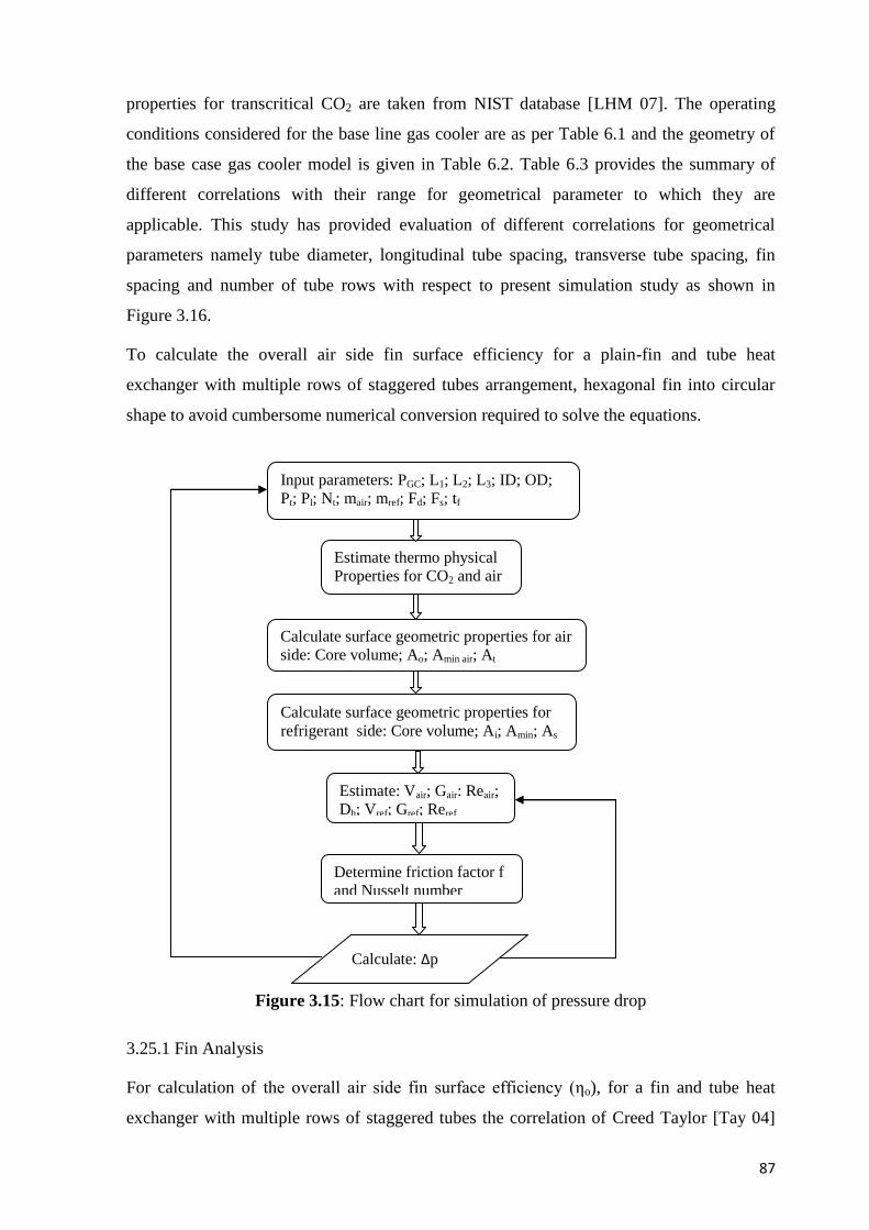
Figure 3.15: Flow chart for simulation of pressure drop

3.25.1 Fin Analysis

For calculation of the overall air side fin surface efficiency (ηo), for a fin and tube heat

exchanger with multiple rows of staggered tubes the correlation of Creed Taylor [Tay 04]

Input parameters: PGC; L1; L2; L3; ID; OD;

Pt; Pl; Nt; mair; mref; Fd; Fs; tf

Estimate thermo physical

Properties for CO2 and air

Calculate surface geometric properties for air

side: Core volume; Ao; Amin air; At

Calculate surface geometric properties for

refrigerant side: Core volume; Ai; Amin; As

Estimate: Vair; Gair: Reair;

Dh; Vref; Gref; Reref

Determine friction factor f

and Nusselt number

Calculate: ∆p

88

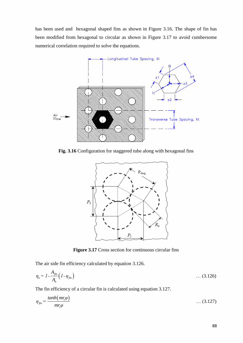
has been used and hexagonal shaped fins as shown in Figure 3.16. The shape of fin has

been modified from hexagonal to circular as shown in Figure 3.17 to avoid cumbersome

numerical correlation required to solve the equations.

Fig. 3.16 Configuration for staggered tube along with hexagonal fins

Figure 3.17 Cross section for continuous circular fins

The air side fin efficiency calculated by equation 3.126.

fin

o fin

o

Aη =1- 1- η

A … (3.126)

The fin efficiency of a circular fin is calculated using equation 3.127.

t

fin

t

tanh mrφη =

mrφ … (3.127)

Pdiag

89

Where, m is the standard extended surface parameter, which is defined as,

o

fin f

2hm =

k .t … (3.128)

The fin efficiency parameter for a circular fin, φ is calculated using equation 3.129.

e e

t t

R Rφ= -1 1+0.35ln

r r

… (3.129)

Where, the equivalent circular fin radius, Re, is calculated using equation 3.130.

t

e l

tt t

XR X2= 1.27 -0.3

Xr r2

… (3.130)

2tdiag l

PP = + P

2

… (3.131)

Rich correlation [Ric 73] is considered to work out air side heat transfer coefficient for the

simulation of air side plain fin and tube gas cooler.

... (3.132)

Air side Nusselt number is calculated by using most familiar Colburn’s equation 3.133.

Colburn

0.3333

u e rN = j.R .P … (3.133)

Based on the experimental data on gas cooling of supercritical carbon dioxide, Yoon et al.

suggested an empirical correlation using the modified form of Dittus-Bolter’s correlation.

The correlation (equation 3.133) suggested by Yoon have an average deviation of 1.6%, the

absolute average deviation of 12.7% and the RMS deviation of 20.2%.

.

0.14, 0.69, 0.66, 0.......

0.013, 1.0, 0.05, 1.6.......

n

pcb c

u e r

pc

pc

N = a.R P

a b c n T T

a b c n T T

… (3.134)

Rich developed plain fin coil correlations for Fanning friction factor based on data from

eight coil configurations (equation 3.135).

-0.5f = 1.70.R ..........3 N 14fins/inr e fL … (3.135)

airR

-0.35j = 0.195* Re

90

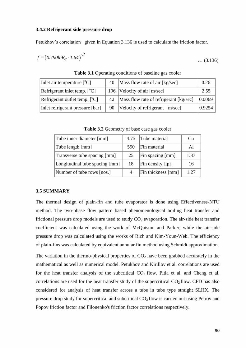
3.4.2 Refrigerant side pressure drop

Petukhov’s correlation given in Equation 3.136 is used to calculate the friction factor.

-2

f = 0.790lnR -1.64e … (3.136)

Table 3.1 Operating conditions of baseline gas cooler

Inlet air temperature [oC] 40 Mass flow rate of air [kg/sec] 0.26

Refrigerant inlet temp. [oC] 106 Velocity of air [m/sec] 2.55

Refrigerant outlet temp. [oC] 42 Mass flow rate of refrigerant [kg/sec] 0.0069

Inlet refrigerant pressure [bar] 90 Velocity of refrigerant [m/sec] 0.9254

Table 3.2 Geometry of base case gas cooler

Tube inner diameter [mm] 4.75 Tube material Cu

Tube length [mm] 550 Fin material Al

Transverse tube spacing [mm] 25 Fin spacing [mm] 1.37

Longitudinal tube spacing [mm] 18 Fin density [fpi] 16

Number of tube rows [nos.] 4 Fin thickness [mm] 1.27

3.5 SUMMARY

The thermal design of plain-fin and tube evaporator is done using Effectiveness-NTU

method. The two-phase flow pattern based phenomenological boiling heat transfer and

frictional pressure drop models are used to study CO2 evaporation. The air-side heat transfer

coefficient was calculated using the work of McQuiston and Parker, while the air-side

pressure drop was calculated using the works of Rich and Kim-Youn-Web. The efficiency

of plain-fins was calculated by equivalent annular fin method using Schmidt approximation.

The variation in the thermo-physical properties of CO2 have been grabbed accurately in the

mathematical as well as numerical model. Petukhov and Kirillov et al. correlations are used

for the heat transfer analysis of the subcritical CO2 flow. Pitla et al. and Cheng et al.

correlations are used for the heat transfer study of the supercritical CO2 flow. CFD has also

considered for analysis of heat transfer across a tube in tube type straight SLHX. The

pressure drop study for supercritical and subcritical CO2 flow is carried out using Petrov and

Popov friction factor and Filonenko's friction factor correlations respectively.

91

A gas cooler is simulated used Microsoft Excel spreadsheet program through one -

dimensional equations. Rich correlations are used for the heat transfer and the pressure drop

study on the air side. Yoon et al. correlation is used refrigerant side heat transfer study and

Petukhon correlation is considered for refrigerant side pressure analysis.

The heat exchangers built through parametric study are later on fine tuned for the

performance and rating in IMST ART considering the overall performance study of the CO2

system.

***