Introduction to Linear Models

Linear models are parametric statistical models that summarize howthe probability distribution of a response variable (usually denoted as Y )depends upon one or more explanatory variables (usually denoted withX’s: X0, X1, X2, . . . , Xk).

• They are statistical (or probabilistic) because they specify a (con-ditional) probability distribution of a random variable (or at leastsome aspects of that distribution, like its mean and variance).

• They are parametric because the probability distribution is specifiedup to a finite number of unknown constants, or parameters.

• They are linear because the mean of the conditional probability dis-tribution of Y , E(Y |X0, X1, . . . , Xk), is specified to be a linear func-tion of model parameters.

• This conditional mean, E(Y |X0, X1, . . . , Xk), is called the regressionfunction for Y on X0, . . . , Xk.

The classical linear model specifies that

Y = X0β0 + X1β1 + · · ·Xkβk + e = xT β + e

where

x =

X0...

Xk

(k+1)×1

, β =

β0...

βk

(k+1)×1

,

where e has conditional mean 0, and variance σ2.

• Notice that this model implies that the regression function is linearin the β’s:

E(Y |x) = X0β0 + X1β1 + · · ·Xkβk.

• Notice that this model indirectly specifies the first two moments ofthe conditional distribution of Y |x by moment assumptions on e:

E(Y |x) = xT β, and var(Y |x) = σ2

2

Strictly speaking, the “model” given above is not a true statistical modelbecause it specifies only the first two moments (i.e., the mean and variance)of Y given x rather than the entire conditional distribution.

Important results concerning the estimation of the regression function,E(Y |x), are available based only on mean and variance specifications.However, for inference on the model parameters, it is necessary to completethe model specification by assuming further that e ∼ N(0, σ2).

• It then follows that Y |x ∼ N(xT β, σ2).

Typically, we will have a sample of data consisting of observed values of nindependent copies of (Y,X0, . . . , Xk):

(Y1, X10, X11, . . . , X1k), . . . , (Yn, Xn0, Xn1, . . . , Xnk).

In this case, the classical linear model is supposed to hold for each copy(Yi, Xi0, Xi1, . . . , Xik), i = 1, . . . , n.

That is, the model becomes

Yi = xTi β + ei, i = 1, . . . , n, where e1, . . . , en

iid∼ N(0, σ2) (∗)

and xi = (Xi0, Xi1, . . . , Xik)T .

• The notation iid∼ N(0, σ2) means, “are independent, identically dis-tributed random variables each with a normal distribution with mean0 and variance σ2.”

• Typically, Xi0 is equal to one for all i in multiple linear regressionmodels, but this need not be so in general.

• In model (*) the parameters are β0, β1, . . . , βk, σ2. The regressionparameters are β0, β1, . . . , βk.

More succinctly, we can write model (*) in vector/matrix notation as

y = Xβ + e, e1, . . . , eniid∼ N(0, σ2).

3

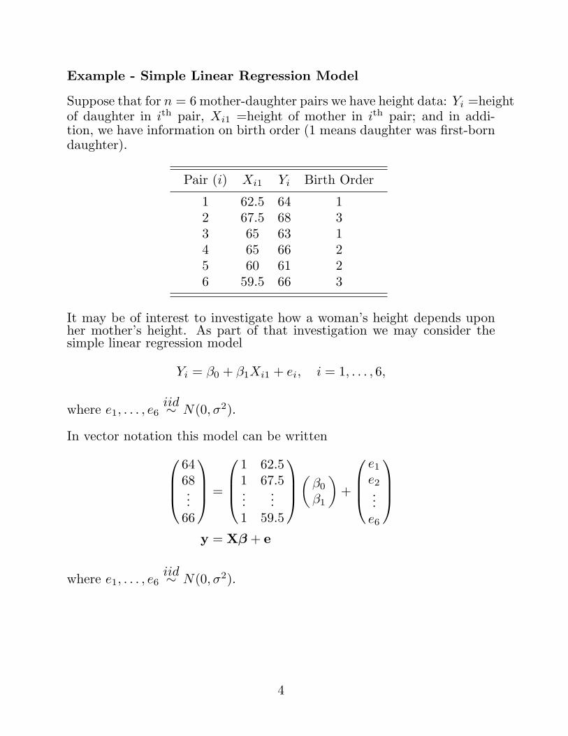
Example - Simple Linear Regression Model

Suppose that for n = 6 mother-daughter pairs we have height data: Yi =heightof daughter in ith pair, Xi1 =height of mother in ith pair; and in addi-tion, we have information on birth order (1 means daughter was first-borndaughter).

Pair (i) Xi1 Yi Birth Order

1 62.5 64 12 67.5 68 33 65 63 14 65 66 25 60 61 26 59.5 66 3

It may be of interest to investigate how a woman’s height depends uponher mother’s height. As part of that investigation we may consider thesimple linear regression model

Yi = β0 + β1Xi1 + ei, i = 1, . . . , 6,

where e1, . . . , e6iid∼ N(0, σ2).

In vector notation this model can be written

6468...

66

=

1 62.51 67.5...

...1 59.5

(β0

β1

)+

e1

e2...e6

y = Xβ + e

where e1, . . . , e6iid∼ N(0, σ2).

4

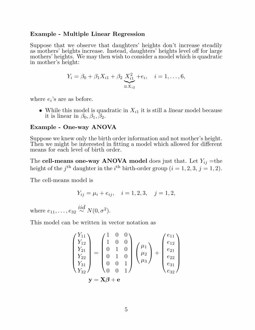
Example - Multiple Linear Regression

Suppose that we observe that daughters’ heights don’t increase steadilyas mothers’ heights increase. Instead, daughters’ heights level off for largemothers’ heights. We may then wish to consider a model which is quadraticin mother’s height:

Yi = β0 + β1Xi1 + β2 X2i1︸︷︷︸

≡Xi2

+ei, i = 1, . . . , 6,

where ei’s are as before.

• While this model is quadratic in Xi1 it is still a linear model becauseit is linear in β0, β1, β2.

Example - One-way ANOVA

Suppose we knew only the birth order information and not mother’s height.Then we might be interested in fitting a model which allowed for differentmeans for each level of birth order.

The cell-means one-way ANOVA model does just that. Let Yij =theheight of the jth daughter in the ith birth-order group (i = 1, 2, 3, j = 1, 2).

The cell-means model is

Yij = µi + eij , i = 1, 2, 3, j = 1, 2,

where e11, . . . , e32iid∼ N(0, σ2).

This model can be written in vector notation as

Y11

Y12

Y21

Y22

Y31

Y32

=

1 0 01 0 00 1 00 1 00 0 10 0 1

µ1

µ2

µ3

+

e11

e12

e21

e22

e31

e32

y = Xβ + e

5

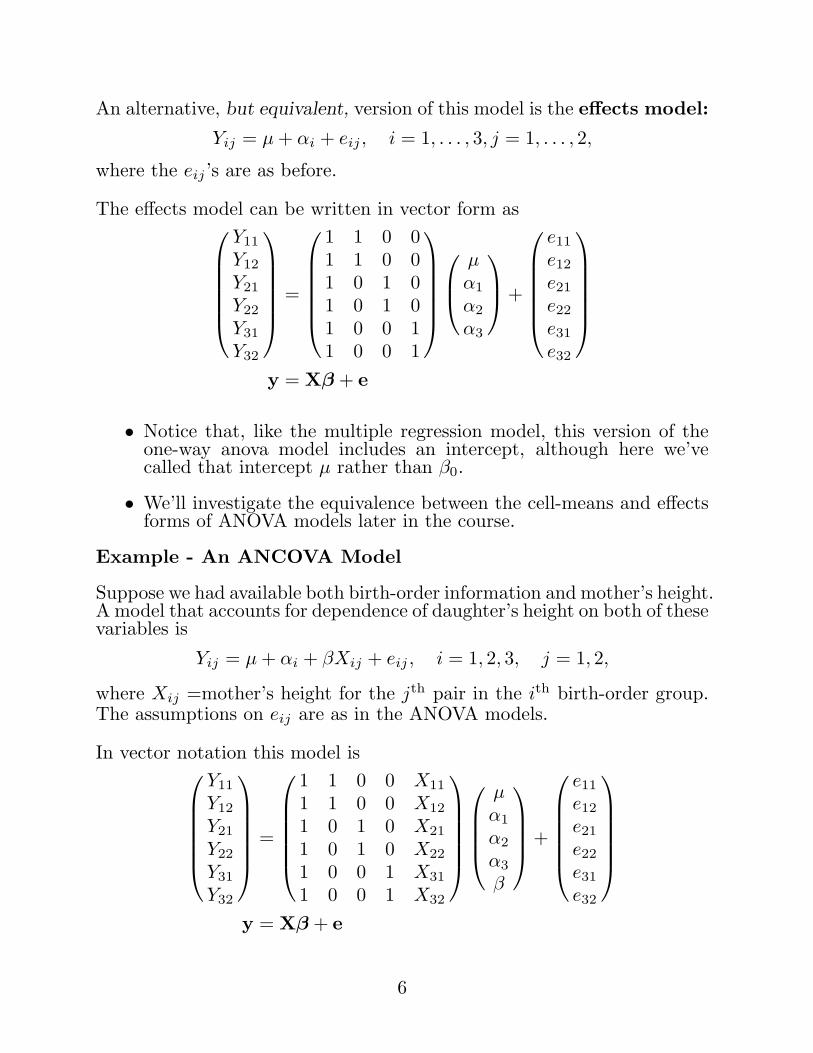
An alternative, but equivalent, version of this model is the effects model:

Yij = µ + αi + eij , i = 1, . . . , 3, j = 1, . . . , 2,

where the eij ’s are as before.

The effects model can be written in vector form as

Y11

Y12

Y21

Y22

Y31

Y32

=

1 1 0 01 1 0 01 0 1 01 0 1 01 0 0 11 0 0 1

µα1

α2

α3

+

e11

e12

e21

e22

e31

e32

y = Xβ + e

• Notice that, like the multiple regression model, this version of theone-way anova model includes an intercept, although here we’vecalled that intercept µ rather than β0.

• We’ll investigate the equivalence between the cell-means and effectsforms of ANOVA models later in the course.

Example - An ANCOVA Model

Suppose we had available both birth-order information and mother’s height.A model that accounts for dependence of daughter’s height on both of thesevariables is

Yij = µ + αi + βXij + eij , i = 1, 2, 3, j = 1, 2,

where Xij =mother’s height for the jth pair in the ith birth-order group.The assumptions on eij are as in the ANOVA models.

In vector notation this model is

Y11

Y12

Y21

Y22

Y31

Y32

=

1 1 0 0 X11

1 1 0 0 X12

1 0 1 0 X21

1 0 1 0 X22

1 0 0 1 X31

1 0 0 1 X32

µα1

α2

α3

β

+

e11

e12

e21

e22

e31

e32

y = Xβ + e

6

In ANOVA models for designed experiments, the explanatory variables(columns of the design matrix X) are fixed by design. That is, they arenon-random.

In regression models, the X’s are often observed simultaneously with theY ’s. That is, they are random variables because they are measured (notassigned or selected) characteristics of the randomly selected unit of ob-servation.

In either case, however, the classical linear model treats X as fixed, byconditioning on the values of the explanatory variables.

That is, the probability distribution of interest is that of Y |x, and allexpectations and variances are conditional on x (e.g., E(Y |x), var(e|x),etc.).

• Because this conditioning applies throughout linear models, we willalways consider the explanatory variables to be constants and we’lloften drop the conditioning notation (the |x part).

• If we have time, we will consider the case where X is considered tobe random later in the course. See ch. 10 of our text.

Notation:

When dealing with scalar-valued random variables, it is common (and use-ful) to use upper and lower case to distinguish between a random variableand the value that it takes on in a given realization.

• E.g., Y, Z are random variables with observed values y, and z, respec-tively. So, we might be concerned with Pr(Z = z) (if Z is discrete),or we might condition on Z = z and consider the conditional meanE(Y |Z = z).

However, when working with vectors and matrices I will drop this distinc-tion and instead denote vectors with bold-faced lower case and matriceswith bold upper case. E.g., y and x are vectors, and X a matrix.

The distinction between the random vector (or matrix) and its realizedvalue will typically be clear from the context.

7

Some Concepts from Linear Algebra

Since our topic is the linear model, its not surprising that many of themost useful mathematical tools come from linear algebra.

Matrices, Vectors, and Matrix Algebra

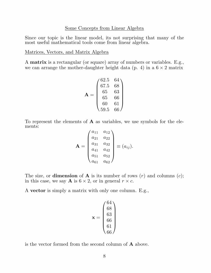
A matrix is a rectangular (or square) array of numbers or variables. E.g.,we can arrange the mother-daughter height data (p. 4) in a 6× 2 matrix

A =

62.5 6467.5 6865 6365 6660 61

59.5 66

To represent the elements of A as variables, we use symbols for the ele-ments:

A =

a11 a12

a21 a22

a31 a32

a41 a42

a51 a52

a61 a62

≡ (aij).

The size, or dimension of A is its number of rows (r) and columns (c);in this case, we say A is 6× 2, or in general r × c.

A vector is simply a matrix with only one column. E.g.,

x =

646863666166

is the vector formed from the second column of A above.

8

• We will typically denote vectors with boldface lower-case letters (e.g.,x,y, z1, etc.) and matrices with boldface upper-case letters (e.g.,A,B,M1,M2, etc.).

• Vectors will always be column vectors. If we need a row vector wewill use the transpose of a vector. E.g., xT = (64, 68, 63, 66, 61, 66)is the row vector version of x.

A scalar is a 1× 1 matrix; i.e., a real-valued number or variable. Scalarswill be denoted in ordinary (non-bold) typeface.

Matrices of special form:

A diagonal matrix is a square matrix with all of its off-diagonal elementsequal to 0. We will use the diag(·) function in two ways: if its argumentis a square matrix, then diag(·) yields a vector formed from the diagonalof that matrix; if its argument is a vector, then diag(·) yields a diagonalmatrix with that vector on the diagonal. E.g.,

diag

1 2 34 5 67 8 9

=

159

diag

123

=

1 0 00 2 00 0 3

.

The n×n identity matrix is a diagonal matrix with 1’s along the diago-nal. We will denote this as I, or In when we want to make clear what thedimension is. E.g.,

I3 =

1 0 00 1 00 0 1

• The identity matrix has the property that

IA = A, BI = B,

where A,B, I are assumed conformable to these multiplications.

A vector of 1’s is denoted as j, or jn when we want to emphasize that thedimension is n. A matrix of 1’s is denoted as J, or Jn,m to emphasize thedimension. E.g.,

j4 = (1, 1, 1, 1)T , J2,3 =(

1 1 11 1 1

).

9

A vector or matrix containing all 0’s will be denoted by 0. Sometimes wewill add subscripts to identify the dimension of this quantity.

Lower and upper-triangular matrices have 0’s above and below the diago-nal, respectively. E.g.,

L =

1 0 02 3 04 5 6

U =

(3 20 1

).

I will assume that you know the basic algebra of vectors and matrices. Inparticular, it is assumed that you are familiar with

• equality/inequality of matrices (two matrices are equal if they havethe same dimension and all corresponding elements are equal);

• matrix addition and subtraction (performed elementwise);• matrix multiplication and conformability (to perform the matrix

multiplication AB, it is necessary for A and B to be conformable;i.e., the number of columns of A must equal the number of rows ofB);

• scalar multiplication (cA is the matrix obtained by multiplying eachelement of A by the scalar c);

• transpose of a matrix (interchange rows and columns, denoted witha T superscript);

• the trace of a square matrix (sum of the diagonal elements; the traceof the n× n matrix A = (aij) is tr(A) =

∑ni=1 aii);

• the determinant of a matrix (a scalar-valued function of a matrixused in computing a matrix inverse; the determinant of A is denoted|A|);

• the inverse of a square matrix A, say (a matrix, denoted A−1, whoseproduct with A yields the identity matrix; i.e., AA−1 = A−1A = I).

• Chapter 2 of our text contains a review of basic matrix algebra.

10

Some Geometric Concepts:

Euclidean Space: A vector(xy

)of dimension two can be thought of as

representing a point on a two-dimensional plane:

and the collection of all such points defines the plane, which we call R2.

Similarly, a three-dimensional vector (x, y, z)T can represent a point in3-dimensional space:

with the collection of all such triples yielding 3 dimensional space, R3.

More generally, Euclidean n-space, denoted Rn, is given by the collectionof all n-tuples (n-dimensional vectors) consisting of real numbers.

• Actually, the proper geometric interpretation of a vector is as a di-rected line segment extending from the origin (the point 0) to thepoint indicated by the coordinates (elements) of the vector.

11

Vector Spaces: Rn (for each possible value of n) is a special case of themore general concept of a vector space:

Let V denote a set of n-dimensional vectors. If, for every pair of vectorsin V , xi ∈ V and xj ∈ V , it is true that

i. xi + xj ∈ V , andii. cxi ∈ V , for all real scalars c,

then V is said to be a vector space of order n.

• Examples: Rn (Euclidean n-space) is a vector space because it isclosed under addition and scalar multiplication. Another exampleis the set consisting only of 0. Moreover, 0 belongs to every vectorspace in Rn.

Spanning Set, Linear Independence, and Basis. The defining char-acteristics of a vector space ensure that all linear combinations of vec-tors in a vector space V are also in V . I.e., if x1, . . . ,xk ∈ V , thenc1x1 + c2x2 + · · ·+ ckxk ∈ V for any scalars c1, . . . , ck.

Suppose that every vector in a vector space V can be expressed as a linearcombination of the k vectors x1, . . . ,xk. Then the set {x1, . . . ,xk} is saidto span or generate V , and we write V = L(x1,x2, . . . ,xk) to denotethat V is the vector space spanned by {x1, . . . ,xk}.

If the spanning set of vectors {x1, . . . ,xk} also has the property of linearindependence, then {x1, . . . ,xk} is called a basis of V .

Vectors x1, . . . ,xk are linearly independent if∑k

i=1 cixi = 0 impliesthat c1 = 0, c2 = 0, . . . , ck = 0.

• I.e., If x1, . . . ,xk are linearly independent (LIN), then there is noredundancy among them in the sense that it is not possible to writex1 (say) as a linear combination of x2, . . . ,xk.

• Therefore, a basis of V is a spanning set that is LIN.

• It is not hard to prove that every basis of a given vector space V hasthe same number of elements. That number of elements is called thedimension or rank of V .

12

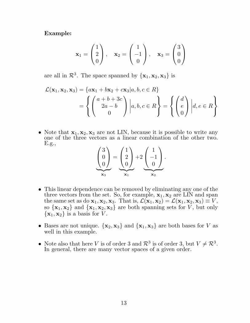
Example:

x1 =

120

, x2 =

1−10

, x3 =

300

are all in R3. The space spanned by {x1,x2,x3} is

L(x1,x2,x3) = {ax1 + bx2 + cx3|a, b, c ∈ R}

=

a + b + 3c2a− b

0

∣∣∣∣a, b, c ∈ R

=

de0

∣∣∣∣d, e ∈ R

• Note that x1,x2,x3 are not LIN, because it is possible to write anyone of the three vectors as a linear combination of the other two.E.g.,

300

︸ ︷︷ ︸x3

=

120

︸ ︷︷ ︸x1

+2

1−10

︸ ︷︷ ︸x2

.

• This linear dependence can be removed by eliminating any one of thethree vectors from the set. So, for example, x1,x2 are LIN and spanthe same set as do x1,x2,x3. That is, L(x1,x2) = L(x1,x2,x3) ≡ V ,so {x1,x2} and {x1,x2,x3} are both spanning sets for V , but only{x1,x2} is a basis for V .

• Bases are not unique. {x2,x3} and {x1,x3} are both bases for V aswell in this example.

• Note also that here V is of order 3 and R3 is of order 3, but V 6= R3.In general, there are many vector spaces of a given order.

13

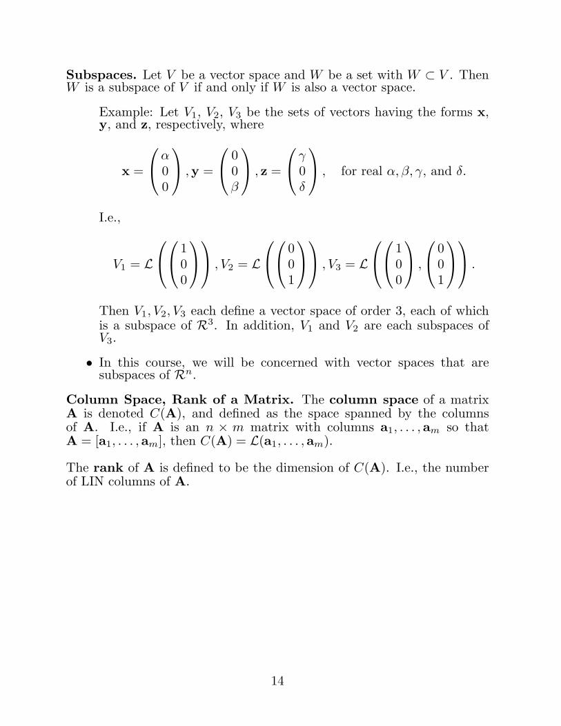
Subspaces. Let V be a vector space and W be a set with W ⊂ V . ThenW is a subspace of V if and only if W is also a vector space.

Example: Let V1, V2, V3 be the sets of vectors having the forms x,y, and z, respectively, where

x =

α00

,y =

00β

, z =

γ0δ

, for real α, β, γ, and δ.

I.e.,

V1 = L

100

, V2 = L

001

, V3 = L

100

,

001

.

Then V1, V2, V3 each define a vector space of order 3, each of whichis a subspace of R3. In addition, V1 and V2 are each subspaces ofV3.

• In this course, we will be concerned with vector spaces that aresubspaces of Rn.

Column Space, Rank of a Matrix. The column space of a matrixA is denoted C(A), and defined as the space spanned by the columnsof A. I.e., if A is an n × m matrix with columns a1, . . . ,am so thatA = [a1, . . . ,am], then C(A) = L(a1, . . . , am).

The rank of A is defined to be the dimension of C(A). I.e., the numberof LIN columns of A.

14

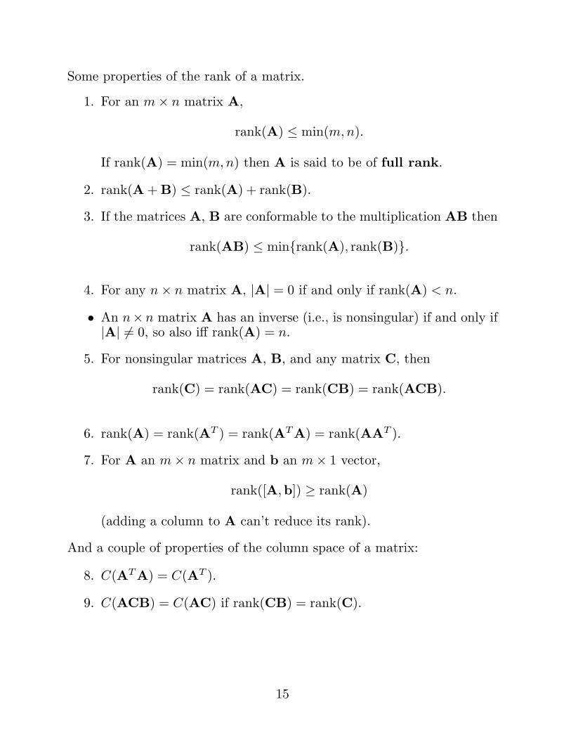
Some properties of the rank of a matrix.

1. For an m× n matrix A,

rank(A) ≤ min(m,n).

If rank(A) = min(m,n) then A is said to be of full rank.

2. rank(A + B) ≤ rank(A) + rank(B).

3. If the matrices A, B are conformable to the multiplication AB then

rank(AB) ≤ min{rank(A), rank(B)}.

4. For any n× n matrix A, |A| = 0 if and only if rank(A) < n.

• An n×n matrix A has an inverse (i.e., is nonsingular) if and only if|A| 6= 0, so also iff rank(A) = n.

5. For nonsingular matrices A, B, and any matrix C, then

rank(C) = rank(AC) = rank(CB) = rank(ACB).

6. rank(A) = rank(AT ) = rank(AT A) = rank(AAT ).

7. For A an m× n matrix and b an m× 1 vector,

rank([A,b]) ≥ rank(A)

(adding a column to A can’t reduce its rank).

And a couple of properties of the column space of a matrix:

8. C(AT A) = C(AT ).

9. C(ACB) = C(AC) if rank(CB) = rank(C).

15

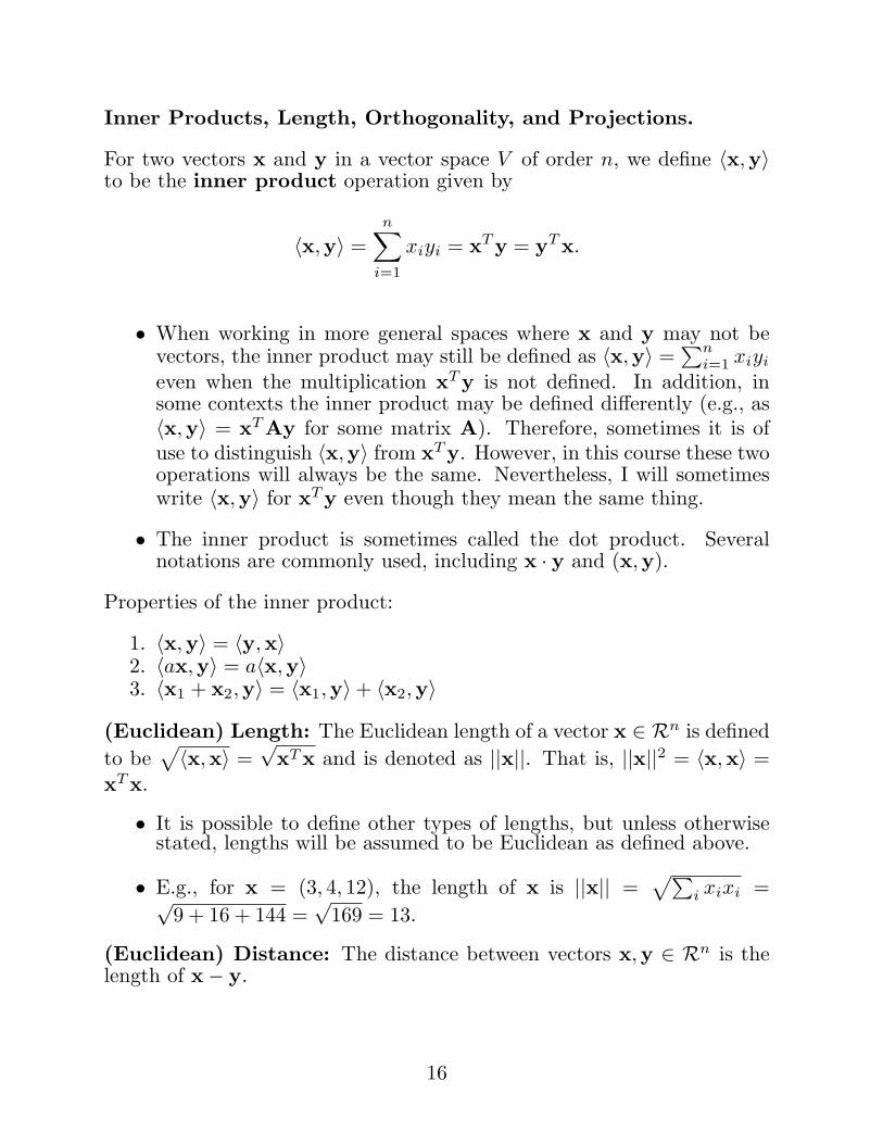
Inner Products, Length, Orthogonality, and Projections.

For two vectors x and y in a vector space V of order n, we define 〈x,y〉to be the inner product operation given by

〈x,y〉 =n∑

i=1

xiyi = xT y = yT x.

• When working in more general spaces where x and y may not bevectors, the inner product may still be defined as 〈x,y〉 =

∑ni=1 xiyi

even when the multiplication xT y is not defined. In addition, insome contexts the inner product may be defined differently (e.g., as〈x,y〉 = xT Ay for some matrix A). Therefore, sometimes it is ofuse to distinguish 〈x,y〉 from xT y. However, in this course these twooperations will always be the same. Nevertheless, I will sometimeswrite 〈x,y〉 for xT y even though they mean the same thing.

• The inner product is sometimes called the dot product. Severalnotations are commonly used, including x · y and (x,y).

Properties of the inner product:

1. 〈x,y〉 = 〈y,x〉2. 〈ax,y〉 = a〈x,y〉3. 〈x1 + x2,y〉 = 〈x1,y〉+ 〈x2,y〉

(Euclidean) Length: The Euclidean length of a vector x ∈ Rn is definedto be

√〈x,x〉 =

√xT x and is denoted as ||x||. That is, ||x||2 = 〈x,x〉 =

xT x.

• It is possible to define other types of lengths, but unless otherwisestated, lengths will be assumed to be Euclidean as defined above.

• E.g., for x = (3, 4, 12), the length of x is ||x|| =√∑

i xixi =√9 + 16 + 144 =

√169 = 13.

(Euclidean) Distance: The distance between vectors x,y ∈ Rn is thelength of x− y.

16

• The inner product between two vectors x,y ∈ Rn quantifies theangle between them. In particular, if θ is the angle formed betweenx and y then

cos(θ) =〈x,y〉||x||||y|| .

Orthogonality: x and y are said to be orthogonal (i.e., perpendicular)if 〈x,y〉 = 0. The orthogonality of x and y is denoted with the notationx ⊥ y.

• Note that orthogonality is a property of a pair of vectors. When wewant to say that each pair in the collection of vectors x1, . . . ,xk isorthogonal, then we say that x1, . . . ,xk are mutually orthogonal.

Example: Consider the model matrix from the ANCOVA example on p.6:

X =

1 1 0 0 62.51 1 0 0 67.51 0 1 0 651 0 1 0 651 0 0 1 601 0 0 1 59.5

Let x1, . . . ,x5 be the columns of X. Then x2 ⊥ x3,x2 ⊥ x4,x3 ⊥ x4 andthe other pairs of vectors are not orthogonal. I.e., x2,x3,x4 are mutuallyorthogonal.

The length of these vectors are

||x1|| =√

12 + 12 + 12 + 12 + 12 + 12 =√

6, ||x2|| = ||x3|| = ||x3|| =√

2,

and||x5|| =

√62.52 + · · ·+ 59.52 = 155.09.

17

Pythagorean Theorem: Let v1, . . . ,vk be mutually orthogonal vectorsin a vector space V . Then

∥∥∥∥∥k∑

i=1

vi

∥∥∥∥∥

2

=k∑

i=1

||vi||2

Proof:

∥∥∥∥∥k∑

i=1

vi

∥∥∥∥∥

2

=

⟨k∑

i=1

vi,k∑

j=1

vj

⟩=

k∑

i=1

k∑

j=1

〈vi,vj〉 =k∑

i=1

〈vi,vi〉 =k∑

i=1

||vi||2

Projections: The (orthogonal) projection of a vector y on a vector xis the vector y such that

1. y = bx for some constant b; and2. (y − y) ⊥ x (or, equivalently, 〈y,x〉 = 〈y,x〉).• It is possible to define non-orthogonal projections, but by default

when we say “projection” we will mean the orthogonal projection asdefined above.

• The notation p(y|x) will denote the projection of y on x.

18

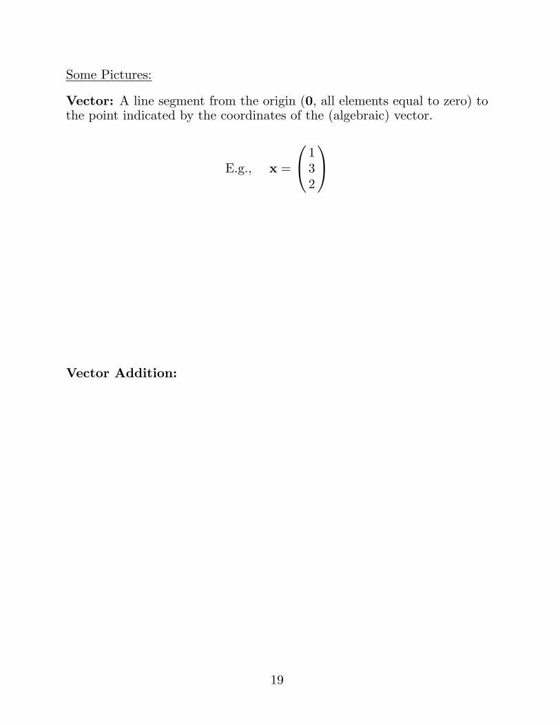
Some Pictures:

Vector: A line segment from the origin (0, all elements equal to zero) tothe point indicated by the coordinates of the (algebraic) vector.

E.g., x =

132

Vector Addition:

19

Scalar Multiplication: Multiplication by a scalar scales a vector byshrinking or extending the vector in the same direction (or opposite direc-tion if the scalar is negative).

Projection: The projection of y on x is the vector in the direction of x(part 1 of the definition) whose difference from y is orthogonal (perpen-dicular) to x (part 2 of the definition).

• From the picture above it is clear that y is the projection of y onthe subspace of all vectors of the form ax, the subspace spanned byx.

20

It is straight-forward to find y = p(y|x), the projection of y on x:

By part 1 of the definition y = bx, and by part 2,

yT x = yT x.

But sinceyT x = (bx)T x = bxT x = b‖x‖2,

the definition implies that

b‖x‖2 = yT x ⇒ b =yT x‖x‖2

unless x = 0, in which case b could be any constant.

So, y is given by

y =

{(any constant)0 = 0, for x = 0(

yT x‖x‖2

)x, otherwise

Example: In R2, let y =(43

), x =

(50

). Then to find y = p(y|x) we

compute xT y = 20, ‖x‖2 = 25, b = 20/25 = 4/5 so that y = bx =(4/5)

(50

)=

(40

).

In addition, y − y =(03

)so y − y ⊥ x.

In this case, the Pythagorean Theorem reduces to its familiar form fromhigh school algebra. The squared length of the hypotenuse (‖y‖2 = 16 +9 = 25) is equal to the sum of the squared lengths of the other two sidesof a right triangle (‖y − y‖2 + ‖y‖2 = 9 + 16 = 25).

21

Theorem Among all multiples ax of x, the projection y = p(y|x) is theclosest vector to y.

Proof: Let y∗ = cx for some constant c. y is such that

(y − y) ⊥ ax for any scalar a

so in particular, for b = yT x/‖x‖2,

(y − y) ⊥ (b− c)x︸ ︷︷ ︸=bx−cx=y−y∗

In addition,y − y∗ = y − y︸ ︷︷ ︸+ y − y∗︸ ︷︷ ︸

so the P.T. implies

‖y − y∗‖2 = ‖y − y‖2 + ‖y − y∗‖2⇒ ‖y − y∗‖2 ≥ ‖y − y‖2 for all y∗ = cx

with equality if and only if y∗ = y.

The same sort of argument establishes the Cauchy-Schwartz Inequal-ity:

Since y ⊥ (y − y) and y = y + (y − y), it follows from the P.T. that

‖y‖2 = ‖y‖2 + ‖y − y‖2= b2‖x‖2 + ‖y − y‖2

=(yT x)2

‖x‖2 + ‖y − y‖2︸ ︷︷ ︸≥0

⇒ ‖y‖2 ≥ (yT x)2

‖x‖2

or(yT x)2 ≤ ‖y‖2‖x‖2

with equality if and only if ‖y − y‖ = 0 (i.e., iff y is a multiple of x).

22

Projections onto 0/1 or indicator vectors. Consider a vector space inRn. Let A be a subset of the indices 1, . . . , n. Let iA denote the indicatorvector for A; that is iA is the n-dimensional vector with 1’s in the positionsgiven in the set A, and 0’s elsewhere.

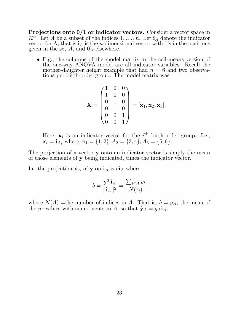
• E.g., the columns of the model matrix in the cell-means version ofthe one-way ANOVA model are all indicator variables. Recall themother-daughter height example that had n = 6 and two observa-tions per birth-order group. The model matrix was

X =

1 0 01 0 00 1 00 1 00 0 10 0 1

= [x1,x2,x3].

Here, xi is an indicator vector for the ith birth-order group. I.e.,xi = iAi where A1 = {1, 2}, A2 = {3, 4}, A3 = {5, 6}.

The projection of a vector y onto an indicator vector is simply the meanof those elements of y being indicated, times the indicator vector.

I.e.,the projection yA of y on iA is biA where

b =yT iA‖iA‖2 =

∑i∈A yi

N(A)

where N(A) =the number of indices in A. That is, b = yA, the mean ofthe y−values with components in A, so that yA = yAiA.

23

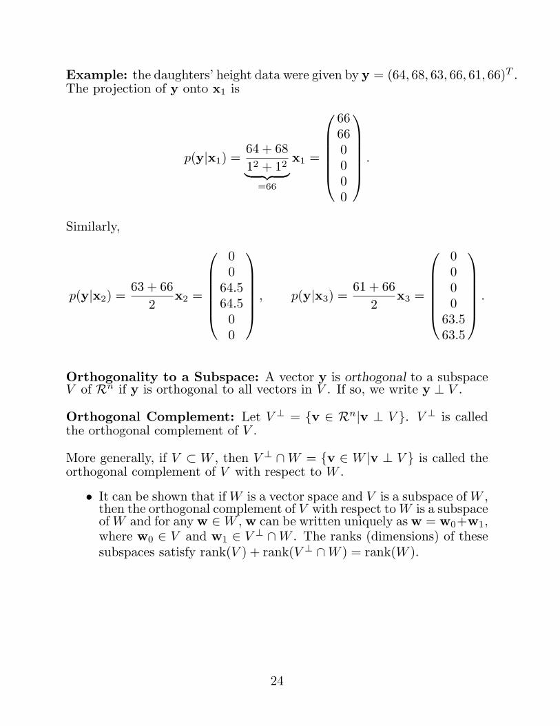
Example: the daughters’ height data were given by y = (64, 68, 63, 66, 61, 66)T .The projection of y onto x1 is

p(y|x1) =64 + 6812 + 12︸ ︷︷ ︸

=66

x1 =

66660000

.

Similarly,

p(y|x2) =63 + 66

2x2 =

00

64.564.500

, p(y|x3) =61 + 66

2x3 =

0000

63.563.5

.

Orthogonality to a Subspace: A vector y is orthogonal to a subspaceV of Rn if y is orthogonal to all vectors in V . If so, we write y ⊥ V .

Orthogonal Complement: Let V ⊥ = {v ∈ Rn|v ⊥ V }. V ⊥ is calledthe orthogonal complement of V .

More generally, if V ⊂ W , then V ⊥ ∩W = {v ∈ W |v ⊥ V } is called theorthogonal complement of V with respect to W .

• It can be shown that if W is a vector space and V is a subspace of W ,then the orthogonal complement of V with respect to W is a subspaceof W and for any w ∈ W , w can be written uniquely as w = w0+w1,where w0 ∈ V and w1 ∈ V ⊥ ∩W . The ranks (dimensions) of thesesubspaces satisfy rank(V ) + rank(V ⊥ ∩W ) = rank(W ).

24

Projection onto a Subspace: The projection of a vector y on a subspaceV of Rn is the vector y ∈ V such that (y− y) ⊥ V . The vector e = y− ywill be called the residual vector for y relative to V .

• Fitting linear models is all about finding projections of a responsevector onto a subspace defined as a linear combination of several vec-tors of explanatory variables. For this reason, the previous definitionis central to this course.

• The condition (y− y) ⊥ V is equivalent to (y− y)T x = 0 or yT x =yT x for all x ∈ V . Therefore, the projection y of y onto V is thevector which has the same inner product as does y with each vectorin V .

Comment: If vectors x1, . . . ,xk span a subspace V then a vector z ∈ Vequals p(y|V ) if 〈z,xi〉 = 〈y,xi〉 for all i.

Why?

Because any vector x ∈ V can be written as∑k

j=1 bjxj for some scalarsb1, . . . , bk, so for any x ∈ V if 〈z,xj〉 = 〈y,xj〉 for all j, then

〈z,x〉 = 〈z,k∑

j=1

bjxj〉 =k∑

j=1

bj〈z,xj〉 =k∑

j=1

bj〈y,xj〉 = 〈y,k∑

j=1

bjxj〉 = 〈y,x〉

Since any vector x in a k−dimensional subspace V can be expressed as alinear combination of basis vectors x1, . . . ,xk, this suggests that we mightbe able to compute the projection y of y on V by summing the projectionsyi = p(y|xi).

• We’ll see that this works, but only if x1, . . . ,xk form an orthogonalbasis for V .

First, does a projection p(y|V ) as we’ve defined it exist at all, and if so,is it unique?

• We do know that a projection onto a one-dimensional subspace existsand is unique. Let V = L(x), for x 6= 0. Then we’ve seen thaty = p(y|V ) is given by

y = p(y|x) =yT x‖x‖2 x.

25

Example Consider R5, the vector space containing all 5−dimensionalvectors of real numbers. Let A1 = {1, 3}, A2 = {2, 5}, A3 = {4} andV = L(iA1 , iA2 , iA3) = C(X), where X is the 5 × 3 matrix with columnsiA1 , iA2 , iA3 .

Let y = (6, 10, 4, 3, 2)T . It is easy to show that the vector

y =3∑

i=1

p(y|iAi) = 5iA1 + 6iA2 + 3iA3 =

56536

satisfies the conditions for a projection onto V (need to check that y ∈ Vand yT iAi = yT iAi , i = 1, 2, 3).

• The representation of y as the sum of projections on linearly inde-pendent vectors spanning V is possible here because iA1 , iA2 , iA3 aremutually orthogonal.

Uniqueness of projection onto a subspace: Suppose y1, y2 are two vectorssatisfying the definition of p(y|V ). Then y1 − y2 ∈ V and

〈y − y1,x〉 = 0 = 〈y − y2,x〉, ∀x ∈ V

⇒ 〈y,x〉 − 〈y1,x〉 = 〈y,x〉 − 〈y2,x〉 ∀x ∈ V

⇒ 〈y1 − y2,x〉 = 0 ∀x ∈ V

so y1 − y2 is orthogonal to all vectors in V including itself, so

‖y1 − y2‖2 = 〈y1 − y2, y1 − y2〉 = 0⇒ y1 − y2 = 0 ⇒ y1 = y2

26

Existence of p(y|V ) is based on showing how to find p(y|V ) if an orthogonalbasis for V exists, and then showing that an orthogonal basis always exists.

Theorem: Let v1, . . . ,vk be an orthogonal basis for V , a subspace of Rk.Then

p(y|V ) =k∑

i=1

p(y|vi).

Proof: Let yi = p(y|vi) = bivi for bi = 〈y,vi〉/‖vi‖2. Since yi is a scalarmultiple of vi, it is orthogonal to vj , j 6= i. From the comment on the topof p.25, we need only show that

∑i yi and y have the same inner product

with each vj . This is true because, for each vj ,

〈∑

i

yi,vj〉 =∑

i

bi〈vi,vj〉 = bj‖vj‖2 = 〈y,vj〉.

Example: Let

y =

633

, v1 =

111

, v2 =

30−3

, V = L(v1,v2).

Then v1 ⊥ v2 and

p(y|V ) = y = p(y|v1) + p(y|v2) =(

123

)v1 +

(918

)v2

=

444

+

3/20

−3/2

=

5.54

2.5

In addition, 〈y,v1〉 = 12, 〈y,v2〉 = 9 are the same as 〈y,v1〉 = 12, and〈y,v2〉 = 16.5 − 7.5 = 9. The residual vector is e = y − y = (.5,−1, .5)T

which is orthogonal to V .

Note that the Pythagorean Theorem holds:

‖y‖2 = 54, ‖y‖2 = 52.5, ‖y − y‖2 = 1.5.

• We will see that this result generalizes to become the decompositionof the total sum of squares into model and error sums of squares ina linear model.

27

Every subspace contains an orthogonal basis (infinitely many, actually).Such a basis can be constructed by the Gram-Schmidt orthogonalizationmethod.

Gram-Schmidt Orthogonalization: Let x1, . . . ,xk be a basis for ak−dimensional subspace V of Rk. For i = 1, . . . , k, let Vi = L(x1, . . . ,xi)so that V1 ⊂ V2 ⊂ · · · ⊂ Vk are nested subspaces. Let

v1 = x1,

v2 = x2 − p(x2|V1) = x2 − p(x2|v1),

v3 = x3 − p(x3|V2) = x3 − {p(x3|v1) + p(x3|v2)},...

vk = xk − p(xk|Vk−1) = xk − {p(xk|v1) + · · ·+ p(xk|vk−1)}

• By construction, v1 ⊥ v2 and v1,v2 span V2; v3 ⊥ V2 (v1,v2,v3

are mutually orthogonal) and v1,v2,v3 span V3; etc., etc., so thatv1, . . . ,vk are mutually orthogonal spanning V .

If v1, . . . ,vk form an orthogonal basis for V , then

y = p(y|V ) =k∑

j=1

p(y|vj) =k∑

j=1

bjvj , where bj = 〈y,vj〉/‖vj‖2

so that the Pythagorean Theorem implies

‖y‖2 =k∑

j=1

‖bjvj‖2 =k∑

j=1

b2j‖vj‖2 =

k∑

j=1

〈y,vj〉2‖vj‖2 .

Orthonormal Basis: Two vectors are said to be orthonormal if they areorthogonal to one another and each has length one.

• Any vector v can be rescaled to have length one simply by multiply-ing that vector by the scalar 1/‖v‖ (dividing by its length).

If v∗1, . . . ,v∗k form an orthonormal basis for V , then the results above

simplify to

y =k∑

j

〈y,v∗j 〉v∗j and ‖y‖2 =k∑

j=1

〈y,v∗j 〉2.

28

Example: The vectors

x1 =

111

, x2 =

100

are a basis for V , the subspace of vectors with the form (a, b, b)T . Toorthonormalize this basis, take v1 = x1, then take

v2 = x2 − p(x2|v1) =

100

− 〈x2,v1〉

‖v1‖2 v1

=

100

− 1

3

111

=

2/3−1/3−1/3

v1,v2 form an orthogonal basis for V , and

v∗1 =1√3v1 =

1/√

31/√

31/√

3

, v∗2 =

1√6/9

v2 =

2/√

6−1/

√6

−1/√

6

form an orthonormal basis for V .

• The Gram-Schmidt method provides a method to find the projectionof y onto the space spanned by any collection of vectors x1, . . . ,xk

(i.e., the column space of any matrix).

• Another method is to solve a matrix equation that contains thek simultaneous linear equations known as the normal equations.This may necessitate the use of a generalized inverse of a matrixif x1, . . . ,xk are linearly dependent (i.e., if the matrix with columnsx1, . . . ,xk is not of full rank).

• See homework #1 for how the Gram-Schmidt approach leads to non-matrix formulas for regression coefficients; in what follows we developthe matrix approach.

29

Consider V = L(x1, . . . ,xk) = C(X), where X = [x1, . . . ,xk]. y, theprojection of y onto V is a vector in V that forms the same angle as doesy with each of the vectors in the spanning set {x1, . . . ,xk}.That is, y has the form y = b1x1 + · · ·+ bkxk where 〈y,xi〉 = 〈y,xi〉, forall i.

These requirements can be expressed as a system of equations, called thenormal equations:

〈y,xi〉 = 〈y,xi〉, i = 1, . . . , k,

or, since y =∑k

j bjxj ,

k∑

j=1

bj〈xj ,xi〉 = 〈y,xi〉, i = 1, . . . , k.

More succinctly, these equations can be written as a single matrix equation:

XT Xb = XT y, (the normal equation)

where b = (b1, . . . , bk)T .

To see this note that XT X has (i, j)th element 〈xi,xj〉 = xTi xj , and XT y

is the k × 1 vector with ith element 〈y,xi〉 = xTi y:

XT X =

xT1

xT2...

xTk

(x1 x2 · · · xk ) = (xT

i xj) and XT y =

xT1

xT2...

xTk

y =

xT1 y

xT2 y...

xTk y

• If XT X has an inverse (is nonsingular) then the equation is easyto solve:

b = (XT X)−1XT y

• Assume X is n × k with n ≥ k. From rank property 6 (p. 15) weknow that

rank(XT X) = rank(X).

Therefore, we conclude that the k × k matrix XT X has full rankk and thus is nonsingular if and only if Xn×k has rank k (has fullcolumn rank or linearly independent columns).

30

If we write y = b1x1 + · · ·+ bkxk = Xb, then for X of full rank we have

y = X(XT X)−1XT y = Py, where P = X(XT X)−1XT

• P = X(XT X)−1XT is called the (orthogonal) projection matrixonto C(X) because premultiplying y by P produces the projectiony = p(y|C(X)).

• P is sometimes called the hat matrix because it “puts the hat on”y. Our book uses the notation H instead of P (‘H’ for hat, ‘P’ forprojection, but these are just two different terms and symbols forthe same thing).

Since y = p(y|C(X)) is the closest point in C(X) to y, b has anotherinterpretation: it is the value of β that makes the linear combination Xβclosest to y. I.e., (for X of full rank) b = (XT X)−1XT y minimizes

Q = ||y −Xβ||2 (the least squares criterion)

31

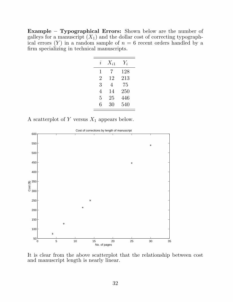
Example – Typographical Errors: Shown below are the number ofgalleys for a manuscript (X1) and the dollar cost of correcting typograph-ical errors (Y ) in a random sample of n = 6 recent orders handled by afirm specializing in technical manuscripts.

i Xi1 Yi

1 7 1282 12 2133 4 754 14 2505 25 4466 30 540

A scatterplot of Y versus X1 appears below.

0 5 10 15 20 25 30 3550

100

150

200

250

300

350

400

450

500

550

600

No. of pages

Cos

t ($)

Cost of corrections by length of manuscript

It is clear from the above scatterplot that the relationship between costand manuscript length is nearly linear.

32

Suppose we try to approximate y = (128, . . . , 540)T by a linear functionb0 + b1x1 where x1 = (7, . . . , 30)T . The problem is to find the values of(β0, β1) in the linear model

y =

1 71 121 41 141 251 30

︸ ︷︷ ︸=X

(β0

β1

)+

e1

e2

e3

e4

e5

e6

y = β0 x0︸︷︷︸=j6

+β1x1 + e.

Projecting y onto L(x0,x1) = C(X) produces y = Xb where b solves thenormal equations

XT Xb = XT y. (∗)

That is, b minimizes

Q = ||y −Xβ||2 = ||y − (β0 + β1x1)||2 = ||e||2 =6∑

i

e2i .

• That is, b minimizes the sum of squared errors. Therefore, Q iscalled the least squares criterion and b is called the least squaresestimator of β.

b solves (*), where

XT X =(

6 9292 1930

)and XT y =

(165234602

)

33

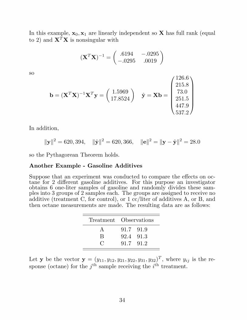
In this example, x0,x1 are linearly independent so X has full rank (equalto 2) and XT X is nonsingular with

(XT X)−1 =(

.6194 −.0295−.0295 .0019

)

so

b = (XT X)−1XT y =(

1.596917.8524

)y = Xb =

126.6215.873.0251.5447.9537.2

In addition,

‖y‖2 = 620, 394, ‖y‖2 = 620, 366, ‖e‖2 = ‖y − y‖2 = 28.0

so the Pythagorean Theorem holds.

Another Example - Gasoline Additives

Suppose that an experiment was conducted to compare the effects on oc-tane for 2 different gasoline additives. For this purpose an investigatorobtains 6 one-liter samples of gasoline and randomly divides these sam-ples into 3 groups of 2 samples each. The groups are assigned to receive noadditive (treatment C, for control), or 1 cc/liter of additives A, or B, andthen octane measurements are made. The resulting data are as follows:

Treatment Observations

A 91.7 91.9B 92.4 91.3C 91.7 91.2

Let y be the vector y = (y11, y12, y21, y22, y31, y32)T , where yij is the re-sponse (octane) for the jth sample receiving the ith treatment.

34

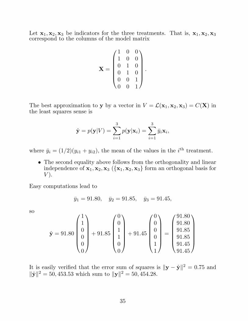
Let x1,x2,x3 be indicators for the three treatments. That is, x1,x2,x3correspond to the columns of the model matrix

X =

1 0 01 0 00 1 00 1 00 0 10 0 1

.

The best approximation to y by a vector in V = L(x1,x2,x3) = C(X) inthe least squares sense is

y = p(y|V ) =3∑

i=1

p(y|xi) =3∑

i=1

yixi,

where yi = (1/2)(yi1 + yi2), the mean of the values in the ith treatment.

• The second equality above follows from the orthogonality and linearindependence of x1,x2,x3 ({x1,x2,x3} form an orthogonal basis forV ).

Easy computations lead to

y1 = 91.80, y2 = 91.85, y3 = 91.45,

so

y = 91.80

110000

+ 91.85

001100

+ 91.45

000011

=

91.8091.8091.8591.8591.4591.45

It is easily verified that the error sum of squares is ‖y − y‖2 = 0.75 and‖y‖2 = 50, 453.53 which sum to ‖y‖2 = 50, 454.28.

35

Projection Matrices.

Definition: P is a (orthogonal) projection matrix onto V if and only if

i. v ∈ V implies Pv = v (projection); andii. w ⊥ V implies Pw = 0 (orthogonality).

• For X an n × k matrix of full rank, it is not hard to show thatP = X(XT X)−1XT satisfies this definition where V = C(X), and istherefore a projection matrix onto C(X). Perhaps simpler though,is to use the following theorem:

Theorem: P is a projection matrix onto its column space C(P) ⊂ Rn ifand only if

i. PP = P (it is idempotent), andii. P = PT (it is symmetric).

Proof: First, the ⇒ part: Choose any two vectors w, z ∈ Rn. w can bewritten w = w1 + w2 where w1 ∈ C(P) and w2 ⊥ C(P) and z can bedecomposed similarly as z = z1 + z2. Note that

(I−P)w = w −Pw = (w1 + w2)−Pw1︸︷︷︸=w1

−Pw2︸︷︷︸=0

= w2

andPz = Pz1 + Pz2 = Pz1 = z1,

so0 = zT

1 w2 = (Pz)T (I−P)w.

We’ve shown that zT PT (I − P)w = 0 for any w, z ∈ Rn, so it must betrue that PT (I − P) = 0 or PT = PT P. Since PT P is symmetric, PT

must also be symmetric, and this implies P = PP.

Second, the ⇐ part: Assume PP = P and P = PT and let v ∈ C(P) andw ⊥ C(P). v ∈ C(P) means that we must be able to write v as Pb forsome vector b. So v = Pb implies Pv = PPb = Pb = v (part i. proved).Now w ⊥ C(P) means that PT w = 0, so Pw = PT w = 0 (proves partii.).

36

Now, for X an n×k matrix of full rank, P = X(XT X)−1XT is a projectionmatrix onto C(P) because it is symmetric:

PT = {X(XT X)−1XT }T = X(XT X)−1XT = P

and idempotent:

PP = {X(XT X)−1XT }{X(XT X)−1XT } = X(XT X)−1XT = P.

Theorem: Projection matrices are unique.

Proof: Let P and M be projection matrices onto some space V . Letx ∈ Rn and write X = v + w where v ∈ V and w ∈ V ⊥. Then Px =Pv + Pw = v and Mx = Mv + Mw = v. So, Px = Mx for any x ∈ Rn.Therefore, P = M.

• Later, we’ll see that C(P) = C(X). This along with the uniquenessof projection matrices means that (in the X of full rank case) P =X(XT X)−1XT is the (unique) projection matrix onto C(X).

So, the projection matrix onto C(X) can be obtained from X as X(XT X)−1XT .Alternatively, the projection matrix onto a subspace can be obtained froman orthonormal basis for the subspace:

Theorem: Let o1, . . . ,ok be an orthonormal basis for V ∈ Rn, and letO = (o1, . . . ,ok). Then OOT =

∑ki=1 oioT

i is the projection matrix ontoV .

Proof: OOT is symmetric and OOT OOT = OOT (idempotent); so, by theprevious theorem OOT is a projection matrix onto C(OOT ) = C(O) = V(using property 8, p.15).

37

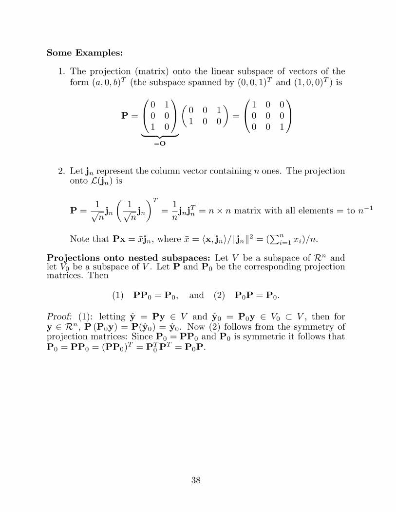
Some Examples:

1. The projection (matrix) onto the linear subspace of vectors of theform (a, 0, b)T (the subspace spanned by (0, 0, 1)T and (1, 0, 0)T ) is

P =

0 10 01 0

︸ ︷︷ ︸=O

(0 0 11 0 0

)=

1 0 00 0 00 0 1

2. Let jn represent the column vector containing n ones. The projectiononto L(jn) is

P =1√njn

(1√njn

)T

=1njnjTn = n× n matrix with all elements = to n−1

Note that Px = xjn, where x = 〈x, jn〉/‖jn‖2 = (∑n

i=1 xi)/n.

Projections onto nested subspaces: Let V be a subspace of Rn andlet V0 be a subspace of V . Let P and P0 be the corresponding projectionmatrices. Then

(1) PP0 = P0, and (2) P0P = P0.

Proof: (1): letting y = Py ∈ V and y0 = P0y ∈ V0 ⊂ V , then fory ∈ Rn, P (P0y) = P(y0) = y0. Now (2) follows from the symmetry ofprojection matrices: Since P0 = PP0 and P0 is symmetric it follows thatP0 = PP0 = (PP0)T = PT

0 PT = P0P.

38

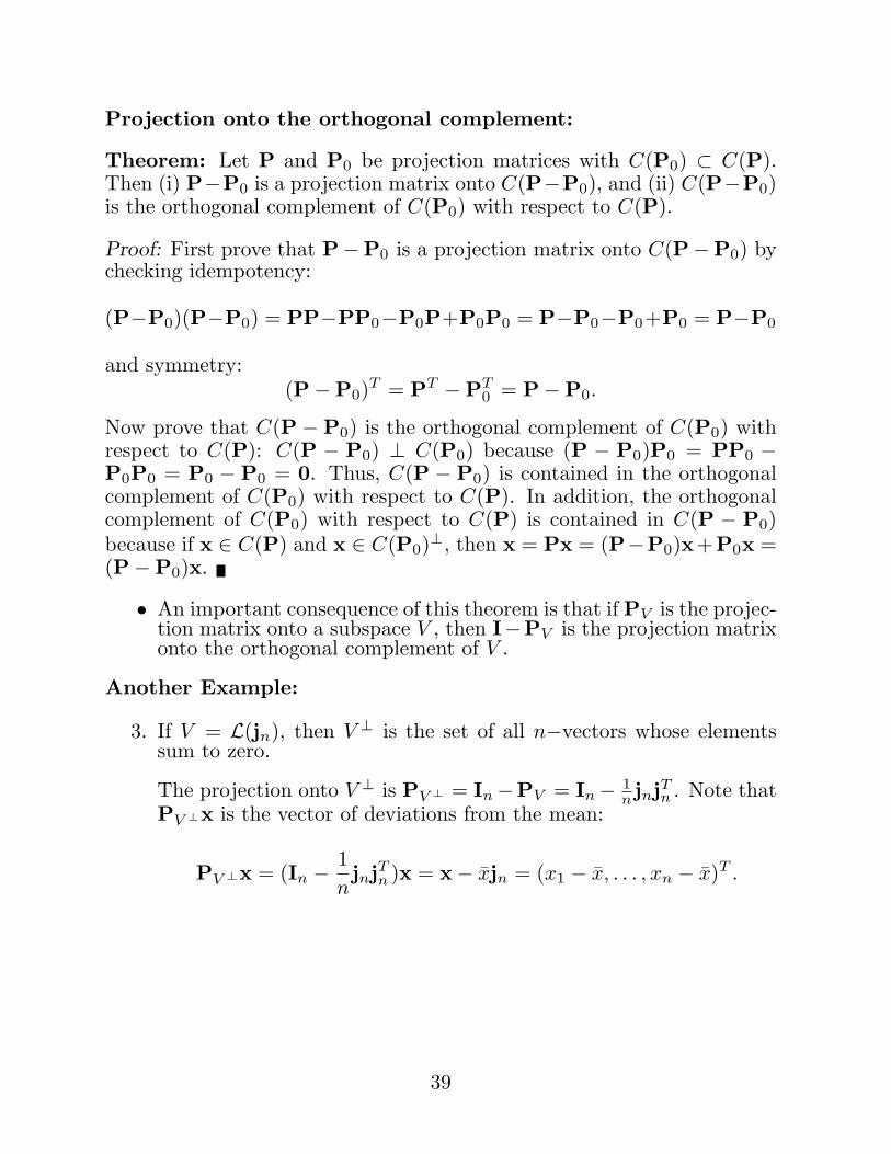
Projection onto the orthogonal complement:

Theorem: Let P and P0 be projection matrices with C(P0) ⊂ C(P).Then (i) P−P0 is a projection matrix onto C(P−P0), and (ii) C(P−P0)is the orthogonal complement of C(P0) with respect to C(P).

Proof: First prove that P−P0 is a projection matrix onto C(P−P0) bychecking idempotency:

(P−P0)(P−P0) = PP−PP0−P0P+P0P0 = P−P0−P0+P0 = P−P0

and symmetry:(P−P0)T = PT −PT

0 = P−P0.

Now prove that C(P − P0) is the orthogonal complement of C(P0) withrespect to C(P): C(P − P0) ⊥ C(P0) because (P − P0)P0 = PP0 −P0P0 = P0 − P0 = 0. Thus, C(P − P0) is contained in the orthogonalcomplement of C(P0) with respect to C(P). In addition, the orthogonalcomplement of C(P0) with respect to C(P) is contained in C(P − P0)because if x ∈ C(P) and x ∈ C(P0)⊥, then x = Px = (P−P0)x+P0x =(P−P0)x.

• An important consequence of this theorem is that if PV is the projec-tion matrix onto a subspace V , then I−PV is the projection matrixonto the orthogonal complement of V .

Another Example:

3. If V = L(jn), then V ⊥ is the set of all n−vectors whose elementssum to zero.

The projection onto V ⊥ is PV ⊥ = In−PV = In− 1n jnjTn . Note that

PV ⊥x is the vector of deviations from the mean:

PV ⊥x = (In − 1njnjTn )x = x− xjn = (x1 − x, . . . , xn − x)T .

39

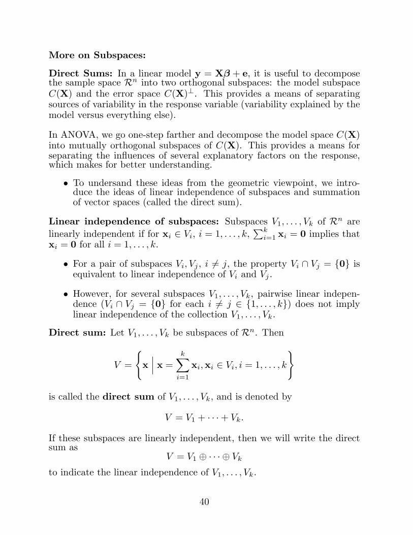
More on Subspaces:

Direct Sums: In a linear model y = Xβ + e, it is useful to decomposethe sample space Rn into two orthogonal subspaces: the model subspaceC(X) and the error space C(X)⊥. This provides a means of separatingsources of variability in the response variable (variability explained by themodel versus everything else).

In ANOVA, we go one-step farther and decompose the model space C(X)into mutually orthogonal subspaces of C(X). This provides a means forseparating the influences of several explanatory factors on the response,which makes for better understanding.

• To undersand these ideas from the geometric viewpoint, we intro-duce the ideas of linear independence of subspaces and summationof vector spaces (called the direct sum).

Linear independence of subspaces: Subspaces V1, . . . , Vk of Rn arelinearly independent if for xi ∈ Vi, i = 1, . . . , k,

∑ki=1 xi = 0 implies that

xi = 0 for all i = 1, . . . , k.

• For a pair of subspaces Vi, Vj , i 6= j, the property Vi ∩ Vj = {0} isequivalent to linear independence of Vi and Vj .

• However, for several subspaces V1, . . . , Vk, pairwise linear indepen-dence (Vi ∩ Vj = {0} for each i 6= j ∈ {1, . . . , k}) does not implylinear independence of the collection V1, . . . , Vk.

Direct sum: Let V1, . . . , Vk be subspaces of Rn. Then

V =

{x

∣∣∣ x =k∑

i=1

xi,xi ∈ Vi, i = 1, . . . , k

}

is called the direct sum of V1, . . . , Vk, and is denoted by

V = V1 + · · ·+ Vk.

If these subspaces are linearly independent, then we will write the directsum as

V = V1 ⊕ · · · ⊕ Vk

to indicate the linear independence of V1, . . . , Vk.

40

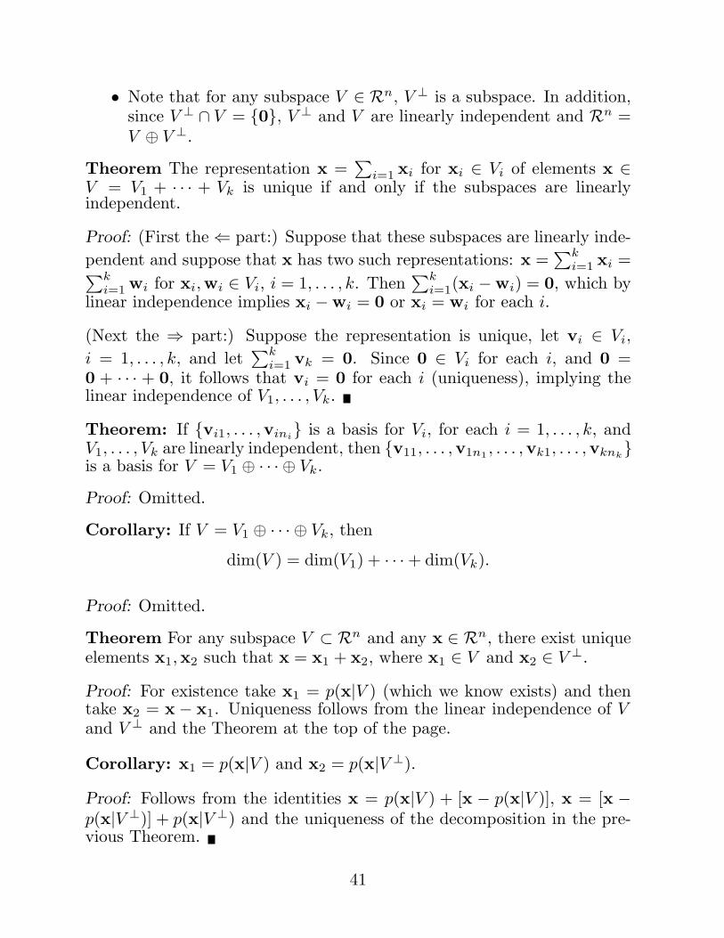
• Note that for any subspace V ∈ Rn, V ⊥ is a subspace. In addition,since V ⊥ ∩ V = {0}, V ⊥ and V are linearly independent and Rn =V ⊕ V ⊥.

Theorem The representation x =∑

i=1 xi for xi ∈ Vi of elements x ∈V = V1 + · · · + Vk is unique if and only if the subspaces are linearlyindependent.

Proof: (First the ⇐ part:) Suppose that these subspaces are linearly inde-pendent and suppose that x has two such representations: x =

∑ki=1 xi =∑k

i=1 wi for xi,wi ∈ Vi, i = 1, . . . , k. Then∑k

i=1(xi −wi) = 0, which bylinear independence implies xi −wi = 0 or xi = wi for each i.

(Next the ⇒ part:) Suppose the representation is unique, let vi ∈ Vi,i = 1, . . . , k, and let

∑ki=1 vk = 0. Since 0 ∈ Vi for each i, and 0 =

0 + · · · + 0, it follows that vi = 0 for each i (uniqueness), implying thelinear independence of V1, . . . , Vk.

Theorem: If {vi1, . . . ,vini} is a basis for Vi, for each i = 1, . . . , k, andV1, . . . , Vk are linearly independent, then {v11, . . . ,v1n1 , . . . ,vk1, . . . ,vknk

}is a basis for V = V1 ⊕ · · · ⊕ Vk.

Proof: Omitted.

Corollary: If V = V1 ⊕ · · · ⊕ Vk, then

dim(V ) = dim(V1) + · · ·+ dim(Vk).

Proof: Omitted.

Theorem For any subspace V ⊂ Rn and any x ∈ Rn, there exist uniqueelements x1,x2 such that x = x1 + x2, where x1 ∈ V and x2 ∈ V ⊥.

Proof: For existence take x1 = p(x|V ) (which we know exists) and thentake x2 = x − x1. Uniqueness follows from the linear independence of Vand V ⊥ and the Theorem at the top of the page.

Corollary: x1 = p(x|V ) and x2 = p(x|V ⊥).

Proof: Follows from the identities x = p(x|V ) + [x − p(x|V )], x = [x −p(x|V ⊥)] + p(x|V ⊥) and the uniqueness of the decomposition in the pre-vious Theorem.

41

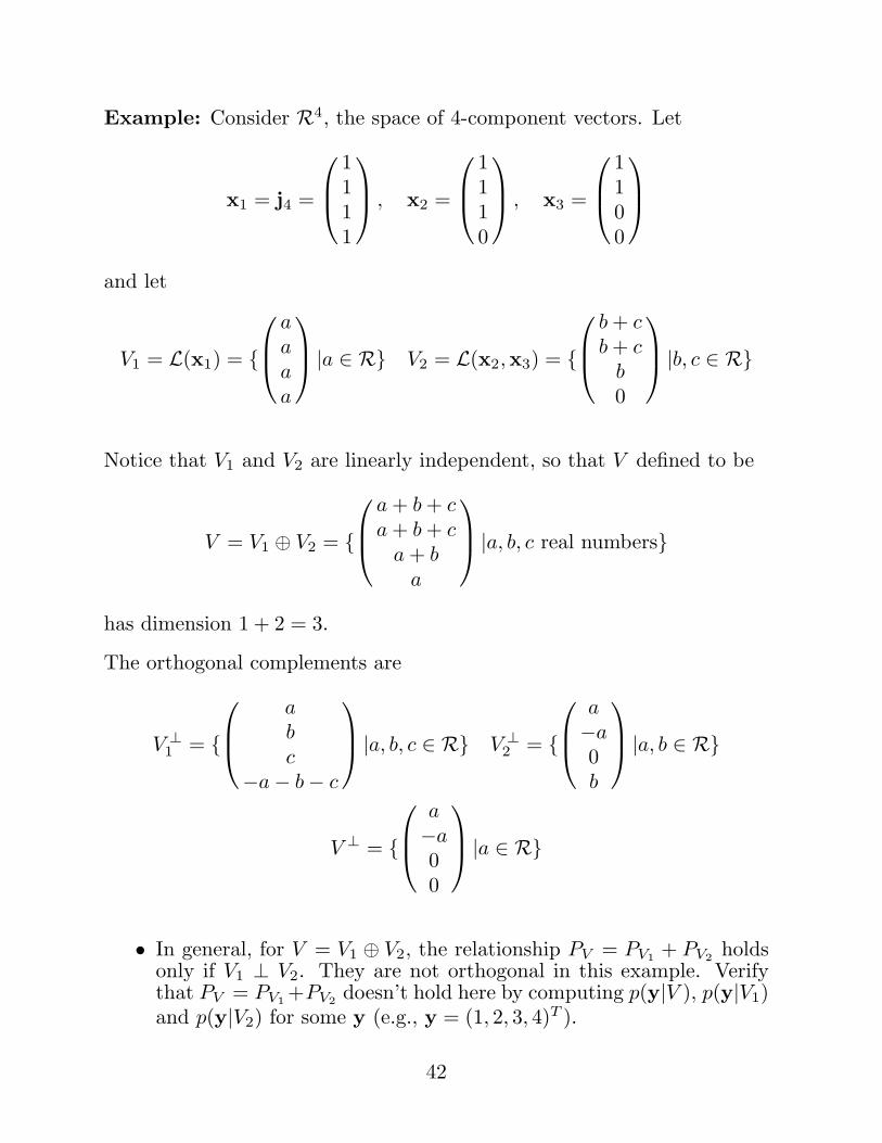
Example: Consider R4, the space of 4-component vectors. Let

x1 = j4 =

1111

, x2 =

1110

, x3 =

1100

and let

V1 = L(x1) = {

aaaa

|a ∈ R} V2 = L(x2,x3) = {

b + cb + c

b0

|b, c ∈ R}

Notice that V1 and V2 are linearly independent, so that V defined to be

V = V1 ⊕ V2 = {

a + b + ca + b + c

a + ba

|a, b, c real numbers}

has dimension 1 + 2 = 3.

The orthogonal complements are

V ⊥1 = {

abc

−a− b− c

|a, b, c ∈ R} V ⊥

2 = {

a−a0b

|a, b ∈ R}

V ⊥ = {

a−a00

|a ∈ R}

• In general, for V = V1 ⊕ V2, the relationship PV = PV1 + PV2 holdsonly if V1 ⊥ V2. They are not orthogonal in this example. Verifythat PV = PV1 +PV2 doesn’t hold here by computing p(y|V ), p(y|V1)and p(y|V2) for some y (e.g., y = (1, 2, 3, 4)T ).

42

Earlier, we established that a projection onto a subspace can be accom-plished by projecting onto orthogonal basis vectors for that subspace andsumming.

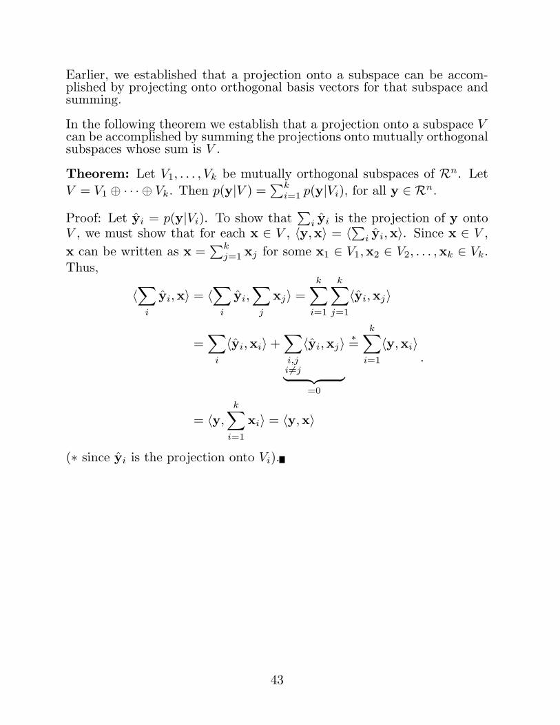
In the following theorem we establish that a projection onto a subspace Vcan be accomplished by summing the projections onto mutually orthogonalsubspaces whose sum is V .

Theorem: Let V1, . . . , Vk be mutually orthogonal subspaces of Rn. LetV = V1 ⊕ · · · ⊕ Vk. Then p(y|V ) =

∑ki=1 p(y|Vi), for all y ∈ Rn.

Proof: Let yi = p(y|Vi). To show that∑

i yi is the projection of y ontoV , we must show that for each x ∈ V , 〈y,x〉 = 〈∑i yi,x〉. Since x ∈ V ,x can be written as x =

∑kj=1 xj for some x1 ∈ V1,x2 ∈ V2, . . . ,xk ∈ Vk.

Thus,

〈∑

i

yi,x〉 = 〈∑

i

yi,∑

j

xj〉 =k∑

i=1

k∑

j=1

〈yi,xj〉

=∑

i

〈yi,xi〉+∑

i,ji6=j

〈yi,xj〉

︸ ︷︷ ︸=0

∗=k∑

i=1

〈y,xi〉

= 〈y,

k∑

i=1

xi〉 = 〈y,x〉

.

(∗ since yi is the projection onto Vi).

43

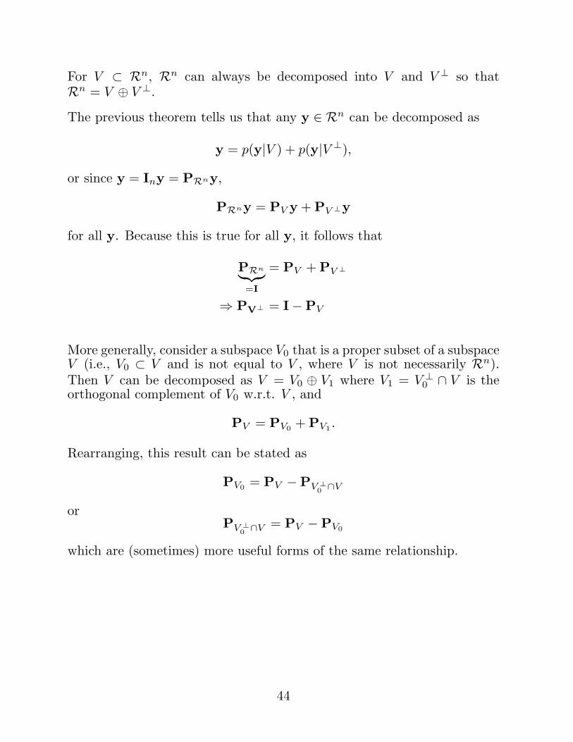
For V ⊂ Rn, Rn can always be decomposed into V and V ⊥ so thatRn = V ⊕ V ⊥.

The previous theorem tells us that any y ∈ Rn can be decomposed as

y = p(y|V ) + p(y|V ⊥),

or since y = Iny = PRny,

PRny = PV y + PV ⊥y

for all y. Because this is true for all y, it follows that

PRn︸︷︷︸=I

= PV + PV ⊥

⇒ PV⊥ = I−PV

More generally, consider a subspace V0 that is a proper subset of a subspaceV (i.e., V0 ⊂ V and is not equal to V , where V is not necessarily Rn).Then V can be decomposed as V = V0 ⊕ V1 where V1 = V ⊥

0 ∩ V is theorthogonal complement of V0 w.r.t. V , and

PV = PV0 + PV1 .

Rearranging, this result can be stated as

PV0 = PV −PV ⊥0 ∩V

orPV ⊥0 ∩V = PV −PV0

which are (sometimes) more useful forms of the same relationship.

44

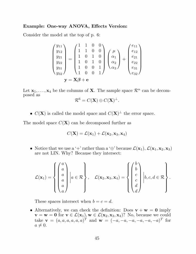
Example: One-way ANOVA, Effects Version:

Consider the model at the top of p. 6:

y11

y12

y21

y22

y31

y32

=

1 1 0 01 1 0 01 0 1 01 0 1 01 0 0 11 0 0 1

µα1

α2

α3

+

e11

e12

e21

e22

e31

e32

y = Xβ + e

Let x1, . . . ,x4 be the columns of X. The sample space Rn can be decom-posed as

R6 = C(X)⊕ C(X)⊥.

• C(X) is called the model space and C(X)⊥ the error space.

The model space C(X) can be decomposed further as

C(X) = L(x1) + L(x2,x3,x4)

• Notice that we use a ‘+’ rather than a ‘⊕’ because L(x1), L(x1,x2,x3)are not LIN. Why? Because they intersect:

L(x1) =

aaaaaa

∣∣∣∣a ∈ R

, L(x2,x3,x4) =

bbccdd

∣∣∣∣b, c, d ∈ R

.

These spaces intersect when b = c = d.

• Alternatively, we can check the definition: Does v + w = 0 implyv = w = 0 for v ∈ L(x1),w ∈ L(x2,x3,x4)? No, because we couldtake v = (a, a, a, a, a, a)T and w = (−a,−a,−a,−a,−a,−a)T fora 6= 0.

45

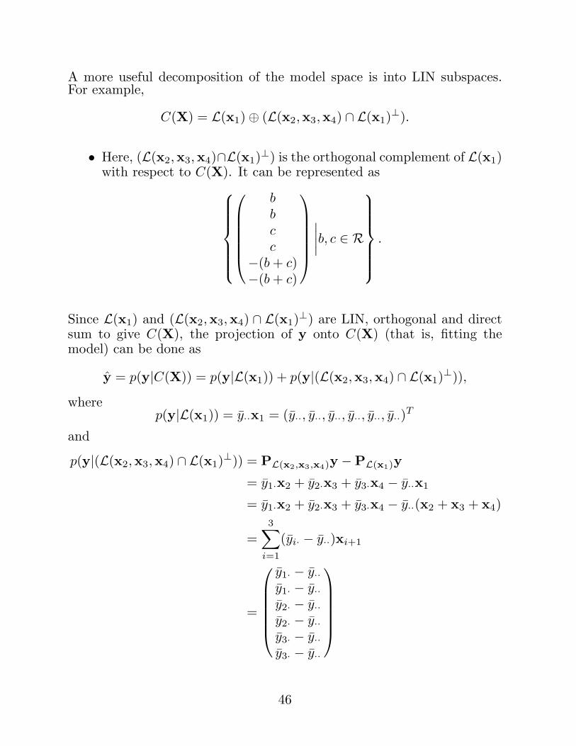
A more useful decomposition of the model space is into LIN subspaces.For example,

C(X) = L(x1)⊕ (L(x2,x3,x4) ∩ L(x1)⊥).

• Here, (L(x2,x3,x4)∩L(x1)⊥) is the orthogonal complement of L(x1)with respect to C(X). It can be represented as

bbcc

−(b + c)−(b + c)

∣∣∣∣b, c ∈ R

.

Since L(x1) and (L(x2,x3,x4) ∩ L(x1)⊥) are LIN, orthogonal and directsum to give C(X), the projection of y onto C(X) (that is, fitting themodel) can be done as

y = p(y|C(X)) = p(y|L(x1)) + p(y|(L(x2,x3,x4) ∩ L(x1)⊥)),

wherep(y|L(x1)) = y··x1 = (y··, y··, y··, y··, y··, y··)T

and

p(y|(L(x2,x3,x4) ∩ L(x1)⊥)) = PL(x2,x3,x4)y −PL(x1)y

= y1·x2 + y2·x3 + y3·x4 − y··x1

= y1·x2 + y2·x3 + y3·x4 − y··(x2 + x3 + x4)

=3∑

i=1

(yi· − y··)xi+1

=

y1· − y··y1· − y··y2· − y··y2· − y··y3· − y··y3· − y··

46

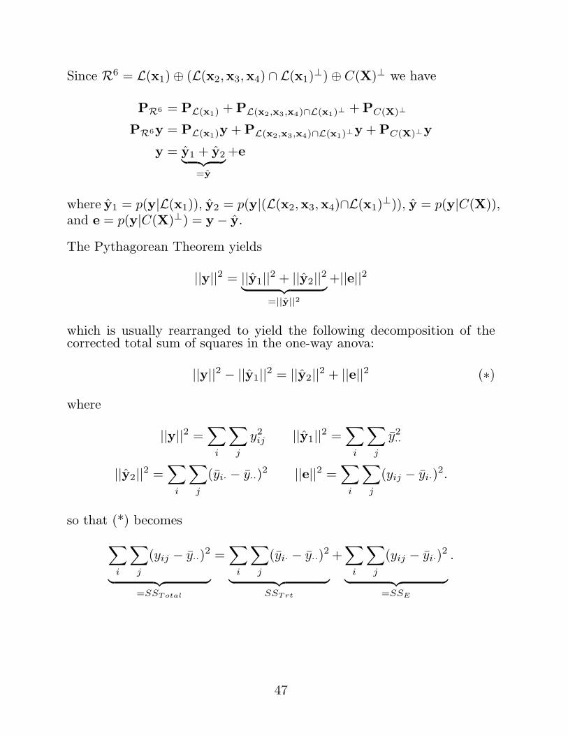
Since R6 = L(x1)⊕ (L(x2,x3,x4) ∩ L(x1)⊥)⊕ C(X)⊥ we have

PR6 = PL(x1) + PL(x2,x3,x4)∩L(x1)⊥ + PC(X)⊥

PR6y = PL(x1)y + PL(x2,x3,x4)∩L(x1)⊥y + PC(X)⊥y

y = y1 + y2︸ ︷︷ ︸=y

+e

where y1 = p(y|L(x1)), y2 = p(y|(L(x2,x3,x4)∩L(x1)⊥)), y = p(y|C(X)),and e = p(y|C(X)⊥) = y − y.

The Pythagorean Theorem yields

||y||2 = ||y1||2 + ||y2||2︸ ︷︷ ︸=||y||2

+||e||2

which is usually rearranged to yield the following decomposition of thecorrected total sum of squares in the one-way anova:

||y||2 − ||y1||2 = ||y2||2 + ||e||2 (∗)

where

||y||2 =∑

i

∑

j

y2ij ||y1||2 =

∑

i

∑

j

y2··

||y2||2 =∑

i

∑

j

(yi· − y··)2 ||e||2 =∑

i

∑

j

(yij − yi·)2.

so that (*) becomes

∑

i

∑

j

(yij − y··)2

︸ ︷︷ ︸=SST otal

=∑

i

∑

j

(yi· − y··)2

︸ ︷︷ ︸SST rt

+∑

i

∑

j

(yij − yi·)2

︸ ︷︷ ︸=SSE

.

47

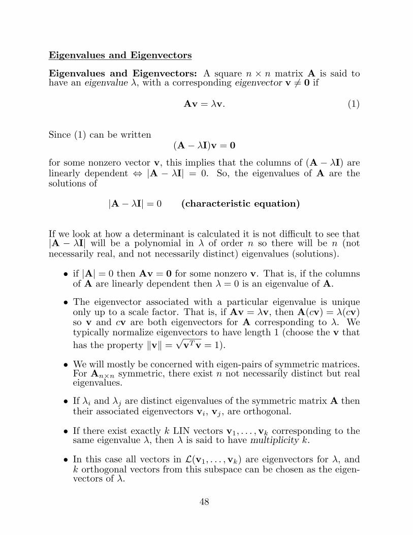
Eigenvalues and Eigenvectors

Eigenvalues and Eigenvectors: A square n × n matrix A is said tohave an eigenvalue λ, with a corresponding eigenvector v 6= 0 if

Av = λv. (1)

Since (1) can be written(A− λI)v = 0

for some nonzero vector v, this implies that the columns of (A − λI) arelinearly dependent ⇔ |A − λI| = 0. So, the eigenvalues of A are thesolutions of

|A− λI| = 0 (characteristic equation)

If we look at how a determinant is calculated it is not difficult to see that|A − λI| will be a polynomial in λ of order n so there will be n (notnecessarily real, and not necessarily distinct) eigenvalues (solutions).

• if |A| = 0 then Av = 0 for some nonzero v. That is, if the columnsof A are linearly dependent then λ = 0 is an eigenvalue of A.

• The eigenvector associated with a particular eigenvalue is uniqueonly up to a scale factor. That is, if Av = λv, then A(cv) = λ(cv)so v and cv are both eigenvectors for A corresponding to λ. Wetypically normalize eigenvectors to have length 1 (choose the v thathas the property ‖v‖ =

√vT v = 1).

• We will mostly be concerned with eigen-pairs of symmetric matrices.For An×n symmetric, there exist n not necessarily distinct but realeigenvalues.

• If λi and λj are distinct eigenvalues of the symmetric matrix A thentheir associated eigenvectors vi, vj , are orthogonal.

• If there exist exactly k LIN vectors v1, . . . ,vk corresponding to thesame eigenvalue λ, then λ is said to have multiplicity k.

• In this case all vectors in L(v1, . . . ,vk) are eigenvectors for λ, andk orthogonal vectors from this subspace can be chosen as the eigen-vectors of λ.

48

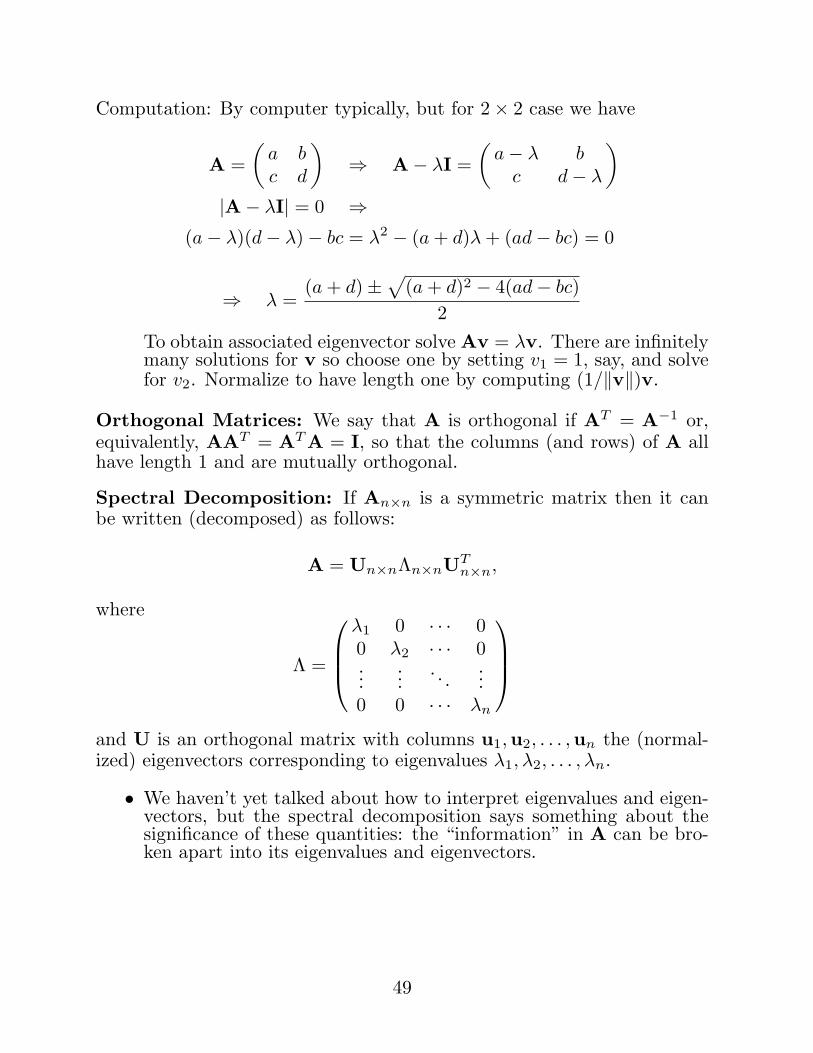
Computation: By computer typically, but for 2× 2 case we have

A =(

a bc d

)⇒ A− λI =

(a− λ b

c d− λ

)

|A− λI| = 0 ⇒(a− λ)(d− λ)− bc = λ2 − (a + d)λ + (ad− bc) = 0

⇒ λ =(a + d)±

√(a + d)2 − 4(ad− bc)

2To obtain associated eigenvector solve Av = λv. There are infinitelymany solutions for v so choose one by setting v1 = 1, say, and solvefor v2. Normalize to have length one by computing (1/‖v‖)v.

Orthogonal Matrices: We say that A is orthogonal if AT = A−1 or,equivalently, AAT = AT A = I, so that the columns (and rows) of A allhave length 1 and are mutually orthogonal.

Spectral Decomposition: If An×n is a symmetric matrix then it canbe written (decomposed) as follows:

A = Un×nΛn×nUTn×n,

where

Λ =

λ1 0 · · · 00 λ2 · · · 0...

.... . .

...0 0 · · · λn

and U is an orthogonal matrix with columns u1,u2, . . . ,un the (normal-ized) eigenvectors corresponding to eigenvalues λ1, λ2, . . . , λn.

• We haven’t yet talked about how to interpret eigenvalues and eigen-vectors, but the spectral decomposition says something about thesignificance of these quantities: the “information” in A can be bro-ken apart into its eigenvalues and eigenvectors.

49

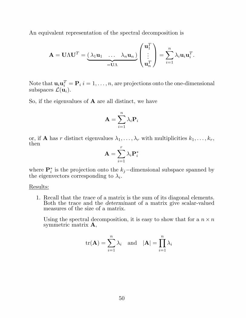
An equivalent representation of the spectral decomposition is

A = UΛUT = ( λ1u1 . . . λnun )︸ ︷︷ ︸=UΛ

uT1...

uTn

=

n∑

i=1

λiuiuTi .

Note that uiuTi = Pi i = 1, . . . , n, are projections onto the one-dimensional

subspaces L(ui).

So, if the eigenvalues of A are all distinct, we have

A =n∑

i=1

λiPi

or, if A has r distinct eigenvalues λ1, . . . , λr with multiplicities k1, . . . , kr,then

A =r∑

i=1

λiP∗i

where P∗i is the projection onto the kj−dimensional subspace spanned bythe eigenvectors corresponding to λi.

Results:

1. Recall that the trace of a matrix is the sum of its diagonal elements.Both the trace and the determinant of a matrix give scalar-valuedmeasures of the size of a matrix.

Using the spectral decomposition, it is easy to show that for a n×nsymmetric matrix A,

tr(A) =n∑

i=1

λi and |A| =n∏

i=1

λi

50

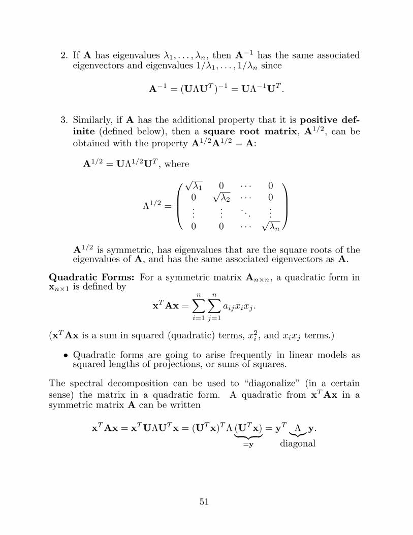
2. If A has eigenvalues λ1, . . . , λn, then A−1 has the same associatedeigenvectors and eigenvalues 1/λ1, . . . , 1/λn since

A−1 = (UΛUT )−1 = UΛ−1UT .

3. Similarly, if A has the additional property that it is positive def-inite (defined below), then a square root matrix, A1/2, can beobtained with the property A1/2A1/2 = A:

A1/2 = UΛ1/2UT , where

Λ1/2 =

√λ1 0 · · · 00

√λ2 · · · 0

......

. . ....

0 0 · · · √λn

A1/2 is symmetric, has eigenvalues that are the square roots of theeigenvalues of A, and has the same associated eigenvectors as A.

Quadratic Forms: For a symmetric matrix An×n, a quadratic form inxn×1 is defined by

xT Ax =n∑

i=1

n∑

j=1

aijxixj .

(xT Ax is a sum in squared (quadratic) terms, x2i , and xixj terms.)

• Quadratic forms are going to arise frequently in linear models assquared lengths of projections, or sums of squares.

The spectral decomposition can be used to “diagonalize” (in a certainsense) the matrix in a quadratic form. A quadratic from xT Ax in asymmetric matrix A can be written

xT Ax = xT UΛUT x = (UT x)T Λ (UT x)︸ ︷︷ ︸=y

= yT Λ︸︷︷︸diagonal

y.

51

Eigen-pairs of Projection Matrices: Suppose that PV is a projection ma-trix onto a subspace V ∈ Rn.

Then for any x ∈ V and any y ∈ V ⊥,

PV x = x = (1)x, and PV y = 0 = (0)y.

Therefore, by definition (see (1) on p.47),

• All vectors in V are eigenvectors of PV with eigenvalues 1, and

• All vectors in V ⊥ are eigenvectors of PV with eigenvalues 0.

• The eigenvalue 1 has multiplicity = dim(V ), and

• The eigenvalue 0 has multiplicity = dim(V ⊥) = n− dim(V ).

• In addition, since tr(A) =∑

i λi it follows that tr(PV ) = dim(V )(the trace of a projection matrix is the dimension of the space ontowhich it projects).

• In addition, rank(PV ) = tr(PV ) = dim(V ).

52

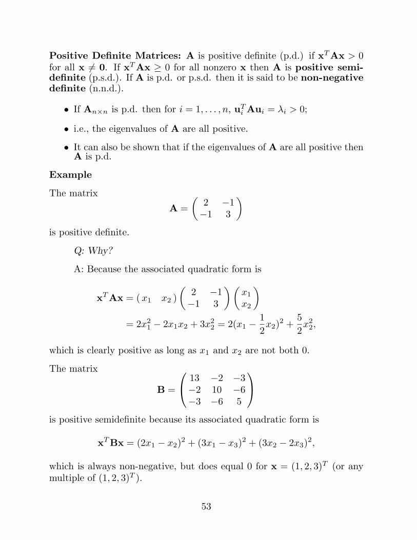
Positive Definite Matrices: A is positive definite (p.d.) if xT Ax > 0for all x 6= 0. If xT Ax ≥ 0 for all nonzero x then A is positive semi-definite (p.s.d.). If A is p.d. or p.s.d. then it is said to be non-negativedefinite (n.n.d.).

• If An×n is p.d. then for i = 1, . . . , n, uTi Aui = λi > 0;

• i.e., the eigenvalues of A are all positive.

• It can also be shown that if the eigenvalues of A are all positive thenA is p.d.

Example

The matrix

A =(

2 −1−1 3

)

is positive definite.

Q: Why?

A: Because the associated quadratic form is

xT Ax = ( x1 x2 )(

2 −1−1 3

)(x1

x2

)

= 2x21 − 2x1x2 + 3x2

2 = 2(x1 − 12x2)2 +

52x2

2,

which is clearly positive as long as x1 and x2 are not both 0.

The matrix

B =

13 −2 −3−2 10 −6−3 −6 5

is positive semidefinite because its associated quadratic form is

xT Bx = (2x1 − x2)2 + (3x1 − x3)2 + (3x2 − 2x3)2,

which is always non-negative, but does equal 0 for x = (1, 2, 3)T (or anymultiple of (1, 2, 3)T ).

53

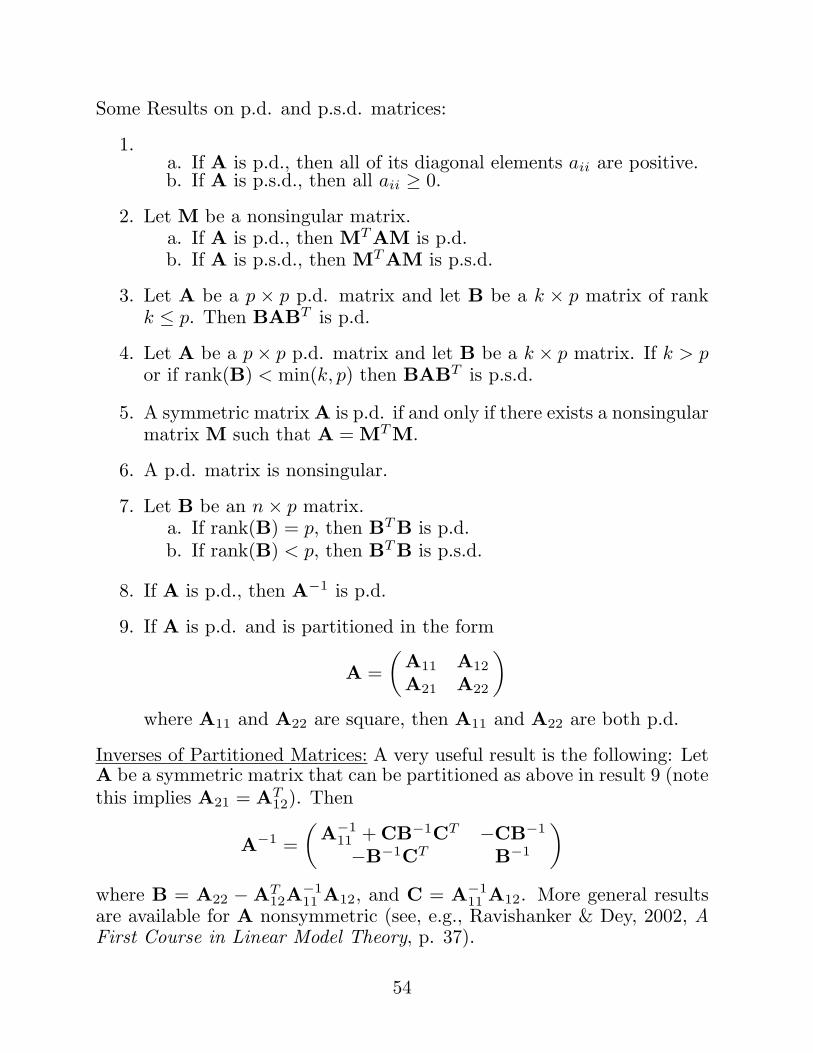
Some Results on p.d. and p.s.d. matrices:

1.a. If A is p.d., then all of its diagonal elements aii are positive.b. If A is p.s.d., then all aii ≥ 0.

2. Let M be a nonsingular matrix.a. If A is p.d., then MT AM is p.d.b. If A is p.s.d., then MT AM is p.s.d.

3. Let A be a p × p p.d. matrix and let B be a k × p matrix of rankk ≤ p. Then BABT is p.d.

4. Let A be a p× p p.d. matrix and let B be a k × p matrix. If k > por if rank(B) < min(k, p) then BABT is p.s.d.

5. A symmetric matrix A is p.d. if and only if there exists a nonsingularmatrix M such that A = MT M.

6. A p.d. matrix is nonsingular.

7. Let B be an n× p matrix.a. If rank(B) = p, then BT B is p.d.b. If rank(B) < p, then BT B is p.s.d.

8. If A is p.d., then A−1 is p.d.

9. If A is p.d. and is partitioned in the form

A =(

A11 A12

A21 A22

)

where A11 and A22 are square, then A11 and A22 are both p.d.

Inverses of Partitioned Matrices: A very useful result is the following: LetA be a symmetric matrix that can be partitioned as above in result 9 (notethis implies A21 = AT

12). Then

A−1 =(

A−111 + CB−1CT −CB−1

−B−1CT B−1

)

where B = A22 −AT12A

−111 A12, and C = A−1

11 A12. More general resultsare available for A nonsymmetric (see, e.g., Ravishanker & Dey, 2002, AFirst Course in Linear Model Theory, p. 37).

54

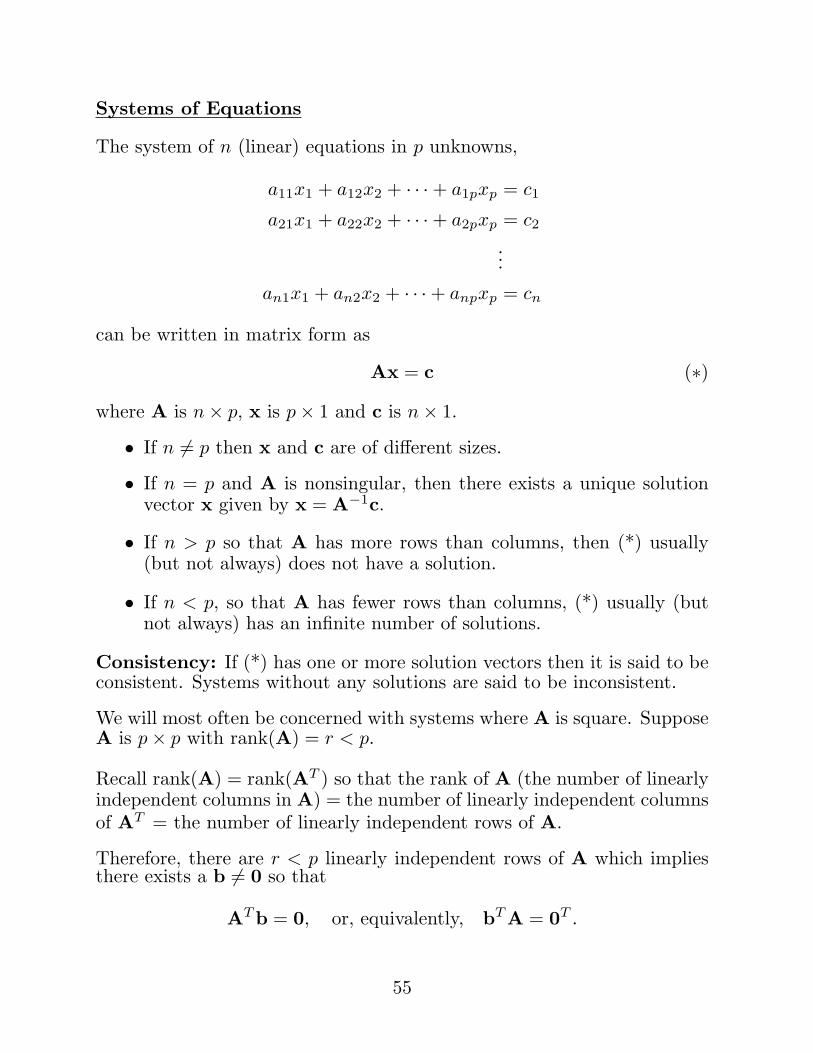
Systems of Equations

The system of n (linear) equations in p unknowns,

a11x1 + a12x2 + · · ·+ a1pxp = c1

a21x1 + a22x2 + · · ·+ a2pxp = c2

...

an1x1 + an2x2 + · · ·+ anpxp = cn

can be written in matrix form as

Ax = c (∗)where A is n× p, x is p× 1 and c is n× 1.

• If n 6= p then x and c are of different sizes.

• If n = p and A is nonsingular, then there exists a unique solutionvector x given by x = A−1c.

• If n > p so that A has more rows than columns, then (*) usually(but not always) does not have a solution.

• If n < p, so that A has fewer rows than columns, (*) usually (butnot always) has an infinite number of solutions.

Consistency: If (*) has one or more solution vectors then it is said to beconsistent. Systems without any solutions are said to be inconsistent.

We will most often be concerned with systems where A is square. SupposeA is p× p with rank(A) = r < p.

Recall rank(A) = rank(AT ) so that the rank of A (the number of linearlyindependent columns in A) = the number of linearly independent columnsof AT = the number of linearly independent rows of A.

Therefore, there are r < p linearly independent rows of A which impliesthere exists a b 6= 0 so that

AT b = 0, or, equivalently, bT A = 0T .

55

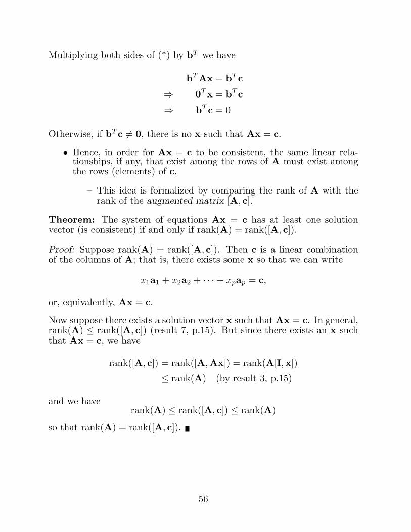
Multiplying both sides of (*) by bT we have

bT Ax = bT c

⇒ 0T x = bT c

⇒ bT c = 0

Otherwise, if bT c 6= 0, there is no x such that Ax = c.

• Hence, in order for Ax = c to be consistent, the same linear rela-tionships, if any, that exist among the rows of A must exist amongthe rows (elements) of c.

– This idea is formalized by comparing the rank of A with therank of the augmented matrix [A, c].

Theorem: The system of equations Ax = c has at least one solutionvector (is consistent) if and only if rank(A) = rank([A, c]).

Proof: Suppose rank(A) = rank([A, c]). Then c is a linear combinationof the columns of A; that is, there exists some x so that we can write

x1a1 + x2a2 + · · ·+ xpap = c,

or, equivalently, Ax = c.

Now suppose there exists a solution vector x such that Ax = c. In general,rank(A) ≤ rank([A, c]) (result 7, p.15). But since there exists an x suchthat Ax = c, we have

rank([A, c]) = rank([A,Ax]) = rank(A[I,x])

≤ rank(A) (by result 3, p.15)

and we haverank(A) ≤ rank([A, c]) ≤ rank(A)

so that rank(A) = rank([A, c]).

56

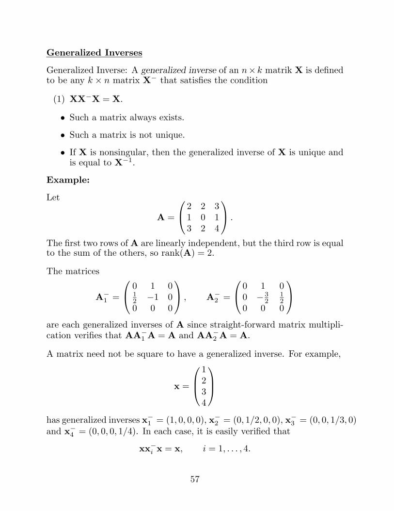
Generalized Inverses

Generalized Inverse: A generalized inverse of an n×k matrik X is definedto be any k × n matrix X− that satisfies the condition

(1) XX−X = X.

• Such a matrix always exists.

• Such a matrix is not unique.

• If X is nonsingular, then the generalized inverse of X is unique andis equal to X−1.

Example:

Let

A =

2 2 31 0 13 2 4

.

The first two rows of A are linearly independent, but the third row is equalto the sum of the others, so rank(A) = 2.

The matrices

A−1 =

0 1 012 −1 00 0 0

, A−

2 =

0 1 00 − 3

212

0 0 0

are each generalized inverses of A since straight-forward matrix multipli-cation verifies that AA−

1 A = A and AA−2 A = A.

A matrix need not be square to have a generalized inverse. For example,

x =

1234

has generalized inverses x−1 = (1, 0, 0, 0), x−2 = (0, 1/2, 0, 0), x−3 = (0, 0, 1/3, 0)and x−4 = (0, 0, 0, 1/4). In each case, it is easily verified that

xx−i x = x, i = 1, . . . , 4.

57

Let X be n× k of rank r, let X− be a generalized inverse of X, and let Gand H be any two generalized inverse of XT X. Then we have the followingresults concerning generalized inverses:

1. rank(X−X) = rank(XX−) = rank(X) = r.

2. (X−)T is a generalized inverse of XT . Furthermore, if X is symmet-ric, then (X−)T is a generalized inverse of X.

3. X = XGXT X = XHXT X.

4. GXT is a generalized inverse of X.

5. XGXT is symmetric, idempotent, and is invariant to the choice ofG; that is, XGXT = XHXT .

Proof:

1. By result 3 on rank (p.15), rank(X−X) ≤ min{rank(X−), rank(X)} ≤rank(X) = r. In addition, because XX−X = X, we have r =rank(X) ≤ min{rank(X), rank(X−X)} ≤ rank(X−X). Putting thesetogether we have r ≤ rank(X−X) ≤ r ⇒ rank(X−X) = r. We canshow rank(XX−) = r similarly.

2. This follows immediately upon transposing both sides of the equationXX−X = X.

3. For v ∈ Rn, let v = v1 + v2 where v1 ∈ C(X) and v2 ⊥ C(X). Letv1 = Xb for some vector b ∈ Rn. Then for any such v,

vT XGXT X = vT1 XGXT X = bT (XT X)G(XT X) = bT (XT X) = vT X.

Since this is true for all v ∈ Rn, it follows that XGXT X = X,and since G is arbitrary and can be replaced by another generalizedinverse H, it follows that XHXT X = X as well.

4. Follows immediately from result 3.

58

5. Invariance: observe that for the arbitrary vector v, above,

XGXT v = XGXT Xb = XHXT Xb = XHXT v.

Since this holds for any v, it follows that XGXT = XHXT .Symmetry: (XGXT )T = XGT XT , but since GT is a generalized in-verse for XT X, the invariance property implies XGT XT = XGXT .Idempotency: XGXT XGXT = XGXT from result 3.

Result 5 says that X(XT X)−XT is symmetric and idempotent for anygeneralized inverse (XT X)−. Therefore, X(XT X)−XT is the unique pro-jection matrix onto C(X(XT X)−XT ).

In addition, C(X(XT X)−XT ) = C(X), because v ∈ C(X(XT X)−XT )⇒ v ∈ C(X), and if v ∈ C(X) then there exists a b ∈ Rn so thatv = Xb = X(XT X)−XT Xb ⇒ v ∈ C(X(XT X)−XT ).

We’ve just proved the following theorem:

Theorem: X(XT X)−XT is the projection matrix onto C(X) (projectionmatrices are uniqe).

• Although a generalized inverse is not unique, this does not poseany particular problem in the theory of linear models, because we’remainly interested in using a generalized inverse to obtain the projec-tion matrix X(XT X)−XT onto C(X), which is unique.

A generalized inverse X− of X which satisfies (1) and has the additionalproperties

(2) X−XX− = X−,(3) X−X is symmetric, and(4) XX− is symmetric,

is unique, and is known as the Moore-Penrose Inverse, but we havelittle use for the Moore-Penrose inverse in this course.

• A generalized inverse of a symmetric matrix is not necessarily sym-metric. However, it is true that a symmetric generalized inverse canalways be found for a symmetric matrix. In this course, we’ll gen-erally assume that generalized inverses of symmetric matrices aresymmetric.

59

Generalized Inverses and Systems of Equations:

A solution to a consistent system of equations can be expressed in termsof a generalized inverse.

Theorem: If the system of equations Ax = c is consistent and if A− isany generalized inverse of A, then x = A−c is a solution.

Proof: Since AA−A = A, we have

AA−Ax = Ax.

Substituting Ax = c on both sides, we obtain

AA−c = c.

Writing this in the form A(A−c) = c, we see that A−c is a solution toAx = c.

For consistent systems of equations with > 1 solution, different choices ofA− will yield different solutions of Ax = c.

Theorem: If the system of equations Ax = c is consistent, then allpossible solutions can be obtained in either of the following two ways:

i. Use a specific A− in the equation x = A−c+(I−A−A)h, combinedwith all possible values of the arbitrary vector h.

ii. Use all possible values of A− in the equation x = A−c.

Proof: See Searle (1982, Matrix Algebra Useful for Statistics, p.238).

60

An alternative necessary and sufficient condition for Ax = c to be consis-tent instead of the rank(A) = rank([A, c]) condition given before is

Theorem: The system of equations Ax = c has a solution if and only iffor any generalized inverse A− of A it is true that

AA−c = c.

Proof: Suppose Ax = c is consistent. Then x = A−c is a solution.Therefore, we can multiply c = Ax by AA− to get

AA−c = AA−Ax = Ax = c.

Now suppose AA−c = c. Then we can multiply x = A−c by A to obtain

Ax = AA−c = c.

Hence a solution exists, namely x = A−c.

The Cholesky Decomposition: Let A be a symmetric positive semi-definite matrix. There exist an infinite number of “square-root matrices”;that is, n× n matrices B such that

A = BT B.

• The matrix square root A1/2 = UΛ1/2UT obtained earlier based onspectral decomposition A = UΛUT is the unique symmetric squareroot, but there are many other non-symmetric square roots.

In particular, there exists a unique upper-triangular matrix B so that thisdecomposition holds. This choice of B is called the Cholesky factor and thedecomposition A = BT B for B upper-triangular is called the Choleskydecomposition.

61

Random Vectors and Matrices

Definitions:

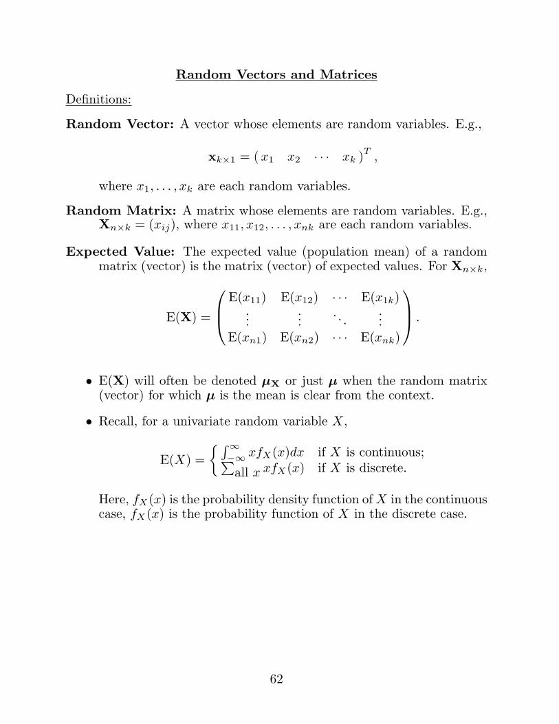
Random Vector: A vector whose elements are random variables. E.g.,

xk×1 = ( x1 x2 · · · xk )T,

where x1, . . . , xk are each random variables.

Random Matrix: A matrix whose elements are random variables. E.g.,Xn×k = (xij), where x11, x12, . . . , xnk are each random variables.

Expected Value: The expected value (population mean) of a randommatrix (vector) is the matrix (vector) of expected values. For Xn×k,

E(X) =

E(x11) E(x12) · · · E(x1k)...

.... . .

...E(xn1) E(xn2) · · · E(xnk)

.

• E(X) will often be denoted µX or just µ when the random matrix(vector) for which µ is the mean is clear from the context.

• Recall, for a univariate random variable X,

E(X) ={ ∫∞

−∞ xfX(x)dx if X is continuous;∑all x xfX(x) if X is discrete.

Here, fX(x) is the probability density function of X in the continuouscase, fX(x) is the probability function of X in the discrete case.

62

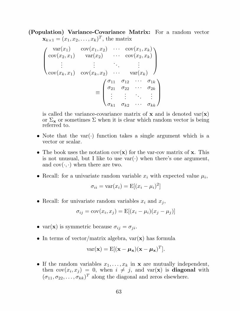
(Population) Variance-Covariance Matrix: For a random vectorxk×1 = (x1, x2, . . . , xk)T , the matrix

var(x1) cov(x1, x2) · · · cov(x1, xk)cov(x2, x1) var(x2) · · · cov(x2, xk)

......

. . ....

cov(xk, x1) cov(xk, x2) · · · var(xk)

≡

σ11 σ12 · · · σ1k

σ21 σ22 · · · σ2k...

.... . .

...σk1 σk2 · · · σkk

is called the variance-covariance matrix of x and is denoted var(x)or Σx or sometimes Σ when it is clear which random vector is beingreferred to.

• Note that the var(·) function takes a single argument which is avector or scalar.

• The book uses the notation cov(x) for the var-cov matrix of x. Thisis not unusual, but I like to use var(·) when there’s one argument,and cov(·, ·) when there are two.

• Recall: for a univariate random variable xi with expected value µi,

σii = var(xi) = E[(xi − µi)2]

• Recall: for univariate random variables xi and xj ,

σij = cov(xi, xj) = E[(xi − µi)(xj − µj)]

• var(x) is symmetric because σij = σji.

• In terms of vector/matrix algebra, var(x) has formula

var(x) = E[(x− µx)(x− µx)T ].

• If the random variables x1, . . . , xk in x are mutually independent,then cov(xi, xj) = 0, when i 6= j, and var(x) is diagonal with(σ11, σ22, . . . , σkk)T along the diagonal and zeros elsewhere.

63

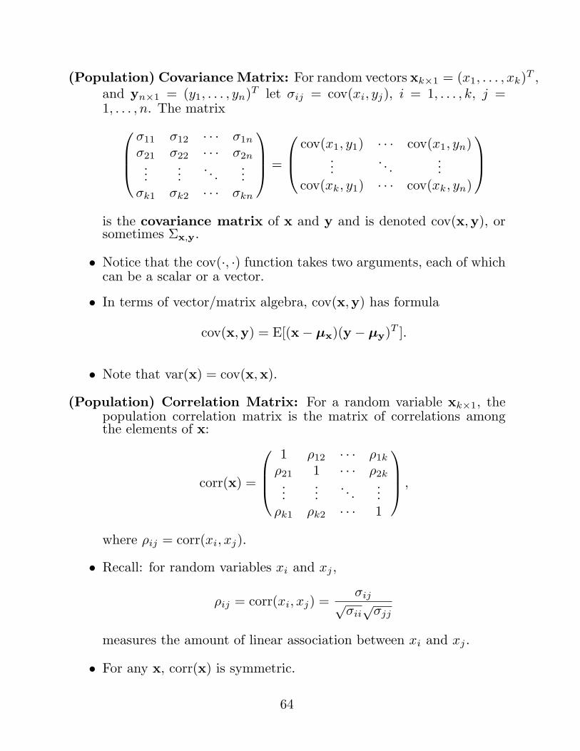
(Population) Covariance Matrix: For random vectors xk×1 = (x1, . . . , xk)T ,and yn×1 = (y1, . . . , yn)T let σij = cov(xi, yj), i = 1, . . . , k, j =1, . . . , n. The matrix

σ11 σ12 · · · σ1n

σ21 σ22 · · · σ2n...

.... . .

...σk1 σk2 · · · σkn

=

cov(x1, y1) · · · cov(x1, yn)...

. . ....

cov(xk, y1) · · · cov(xk, yn)

is the covariance matrix of x and y and is denoted cov(x,y), orsometimes Σx,y.

• Notice that the cov(·, ·) function takes two arguments, each of whichcan be a scalar or a vector.

• In terms of vector/matrix algebra, cov(x,y) has formula

cov(x,y) = E[(x− µx)(y − µy)T ].

• Note that var(x) = cov(x,x).

(Population) Correlation Matrix: For a random variable xk×1, thepopulation correlation matrix is the matrix of correlations amongthe elements of x:

corr(x) =

1 ρ12 · · · ρ1k

ρ21 1 · · · ρ2k...

.... . .

...ρk1 ρk2 · · · 1

,

where ρij = corr(xi, xj).

• Recall: for random variables xi and xj ,

ρij = corr(xi, xj) =σij√

σii√

σjj

measures the amount of linear association between xi and xj .

• For any x, corr(x) is symmetric.

64

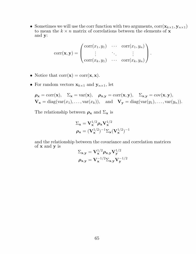
• Sometimes we will use the corr function with two arguments, corr(xk×1,yn×1)to mean the k × n matrix of correlations between the elements of xand y:

corr(x,y) =

corr(x1, y1) · · · corr(x1, yn)...

. . ....

corr(xk, y1) · · · corr(xk, yn)

.

• Notice that corr(x) = corr(x,x).

• For random vectors xk×1 and yn×1, let

ρx = corr(x), Σx = var(x), ρx,y = corr(x,y), Σx,y = cov(x,y),Vx = diag(var(x1), . . . , var(xk)), and Vy = diag(var(y1), . . . , var(yn)).

The relationship between ρx and Σx is

Σx = V1/2x ρxV1/2

x

ρx = (V1/2x )−1Σx(V1/2

x )−1

and the relationship between the covariance and correlation matricesof x and y is

Σx,y = V1/2x ρx,yV1/2

y

ρx,y = V−1/2x Σx,yV−1/2

y

65

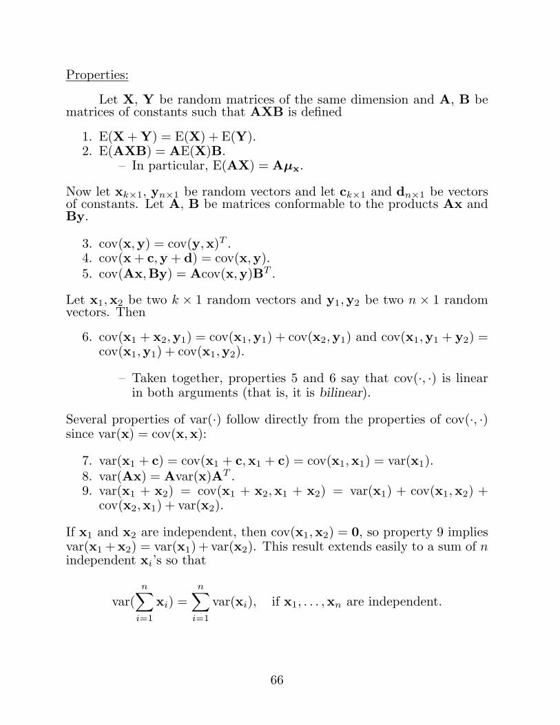
Properties:

Let X, Y be random matrices of the same dimension and A, B bematrices of constants such that AXB is defined

1. E(X + Y) = E(X) + E(Y).2. E(AXB) = AE(X)B.

– In particular, E(AX) = Aµx.

Now let xk×1, yn×1 be random vectors and let ck×1 and dn×1 be vectorsof constants. Let A, B be matrices conformable to the products Ax andBy.

3. cov(x,y) = cov(y,x)T .4. cov(x + c,y + d) = cov(x,y).5. cov(Ax,By) = Acov(x,y)BT .

Let x1,x2 be two k × 1 random vectors and y1,y2 be two n × 1 randomvectors. Then

6. cov(x1 + x2,y1) = cov(x1,y1) + cov(x2,y1) and cov(x1,y1 + y2) =cov(x1,y1) + cov(x1,y2).

– Taken together, properties 5 and 6 say that cov(·, ·) is linearin both arguments (that is, it is bilinear).

Several properties of var(·) follow directly from the properties of cov(·, ·)since var(x) = cov(x,x):

7. var(x1 + c) = cov(x1 + c,x1 + c) = cov(x1,x1) = var(x1).8. var(Ax) = Avar(x)AT .9. var(x1 + x2) = cov(x1 + x2,x1 + x2) = var(x1) + cov(x1,x2) +

cov(x2,x1) + var(x2).

If x1 and x2 are independent, then cov(x1,x2) = 0, so property 9 impliesvar(x1 +x2) = var(x1) + var(x2). This result extends easily to a sum of nindependent xi’s so that

var(n∑

i=1

xi) =n∑

i=1

var(xi), if x1, . . . ,xn are independent.

66

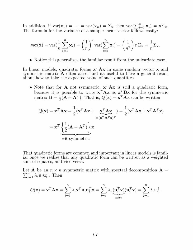
In addition, if var(x1) = · · · = var(xn) = Σx then var(∑n

i=1 xi) = nΣx.The formula for the variance of a sample mean vector follows easily:

var(x) = var(1n

n∑

i=1

xi) =(

1n

)2

var(n∑

i=1

xi) =(

1n2

)nΣx =

1n

Σx.

• Notice this generalizes the familiar result from the univariate case.

In linear models, quadratic forms xT Ax in some random vector x andsymmetric matrix A often arise, and its useful to have a general resultabout how to take the expected value of such quantities.

• Note that for A not symmetric, xT Ax is still a quadratic form,because it is possible to write xT Ax as xT Bx for the symmetricmatrix B = 1

2 (A + AT ). That is, Q(x) = xT Ax can be written

Q(x) = xT Ax =12(xT Ax + xT Ax︸ ︷︷ ︸

=(xT AT x)T

) =12(xT Ax + xT AT x)

= xT

{12(A + AT )

}

︸ ︷︷ ︸=B symmetric

x

That quadratic forms are common and important in linear models is famil-iar once we realize that any quadratic form can be written as a weightedsum of squares, and vice versa.

Let A be an n × n symmetric matrix with spectral decomposition A =∑ni=1 λiuiuT

i . Then

Q(x) = xT Ax =n∑

i=1

λixT uiuTi x =

n∑

i=1

λi (uTi x)︸ ︷︷ ︸≡wi

(uTi x) =

n∑

i=1

λiw2i .

67

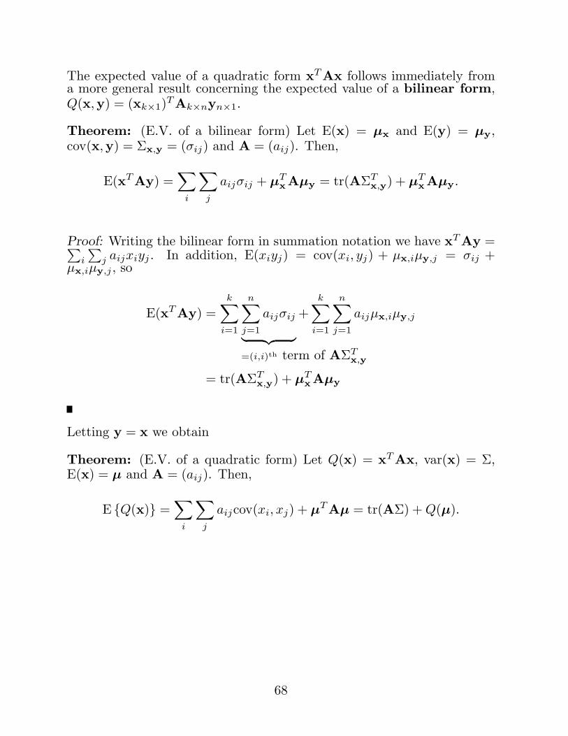
The expected value of a quadratic form xT Ax follows immediately froma more general result concerning the expected value of a bilinear form,Q(x,y) = (xk×1)T Ak×nyn×1.

Theorem: (E.V. of a bilinear form) Let E(x) = µx and E(y) = µy,cov(x,y) = Σx,y = (σij) and A = (aij). Then,

E(xT Ay) =∑

i

∑

j

aijσij + µTxAµy = tr(AΣT

x,y) + µTxAµy.

Proof: Writing the bilinear form in summation notation we have xT Ay =∑i

∑j aijxiyj . In addition, E(xiyj) = cov(xi, yj) + µx,iµy,j = σij +

µx,iµy,j , so

E(xT Ay) =k∑

i=1

n∑

j=1

aijσij

︸ ︷︷ ︸=(i,i)th term of AΣT

x,y

+k∑

i=1

n∑

j=1

aijµx,iµy,j

= tr(AΣTx,y) + µT

xAµy

Letting y = x we obtain

Theorem: (E.V. of a quadratic form) Let Q(x) = xT Ax, var(x) = Σ,E(x) = µ and A = (aij). Then,

E {Q(x)} =∑

i

∑

j

aijcov(xi, xj) + µT Aµ = tr(AΣ) + Q(µ).

68

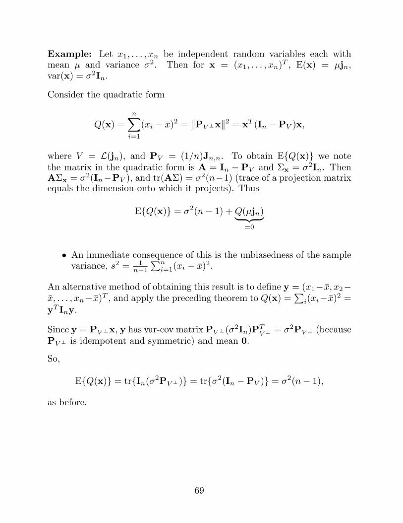
Example: Let x1, . . . , xn be independent random variables each withmean µ and variance σ2. Then for x = (x1, . . . , xn)T , E(x) = µjn,var(x) = σ2In.

Consider the quadratic form

Q(x) =n∑

i=1

(xi − x)2 = ‖PV ⊥x‖2 = xT (In −PV )x,

where V = L(jn), and PV = (1/n)Jn,n. To obtain E{Q(x)} we notethe matrix in the quadratic form is A = In − PV and Σx = σ2In. ThenAΣx = σ2(In−PV ), and tr(AΣ) = σ2(n−1) (trace of a projection matrixequals the dimension onto which it projects). Thus

E{Q(x)} = σ2(n− 1) + Q(µjn)︸ ︷︷ ︸=0

• An immediate consequence of this is the unbiasedness of the samplevariance, s2 = 1

n−1

∑ni=1(xi − x)2.

An alternative method of obtaining this result is to define y = (x1−x, x2−x, . . . , xn−x)T , and apply the preceding theorem to Q(x) =

∑i(xi−x)2 =

yT Iny.

Since y = PV ⊥x, y has var-cov matrix PV ⊥(σ2In)PTV ⊥ = σ2PV ⊥ (because

PV ⊥ is idempotent and symmetric) and mean 0.

So,

E{Q(x)} = tr{In(σ2PV ⊥)} = tr{σ2(In −PV )} = σ2(n− 1),

as before.

69

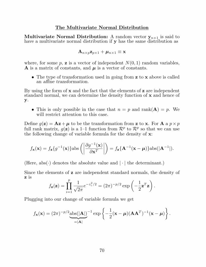
The Multivariate Normal Distribution

Multivariate Normal Distribution: A random vector yn×1 is said tohave a multivariate normal distribution if y has the same distribution as

An×pzp×1 + µn×1 ≡ x

where, for some p, z is a vector of independent N(0, 1) random variables,A is a matrix of constants, and µ is a vector of constants.

• The type of transformation used in going from z to x above is calledan affine transformation.

By using the form of x and the fact that the elements of z are independentstandard normal, we can determine the density function of x and hence ofy.

• This is only possible in the case that n = p and rank(A) = p. Wewill restrict attention to this case.

Define g(z) = Az+µ to be the transformation from z to x. For A a p× pfull rank matrix, g(z) is a 1–1 function from Rp to Rp so that we can usethe following change of variable formula for the density of x:

fx(x) = fz{g−1(x)}abs(∣∣∣∣

∂g−1(x)∂xT

∣∣∣∣)

= fz{A−1(x− µ)}abs(|A−1|).

(Here, abs(·) denotes the absolute value and | · | the determinant.)

Since the elements of z are independent standard normals, the density ofz is

fz(z) =p∏

i=1

1√2π

e−z2i /2 = (2π)−p/2 exp

(−1

2zT z

).

Plugging into our change of variable formula we get

fx(x) = (2π)−p/2abs(|A|)︸ ︷︷ ︸=|A|

−1 exp{−1

2(x− µ)(AAT )−1(x− µ)

}.

70

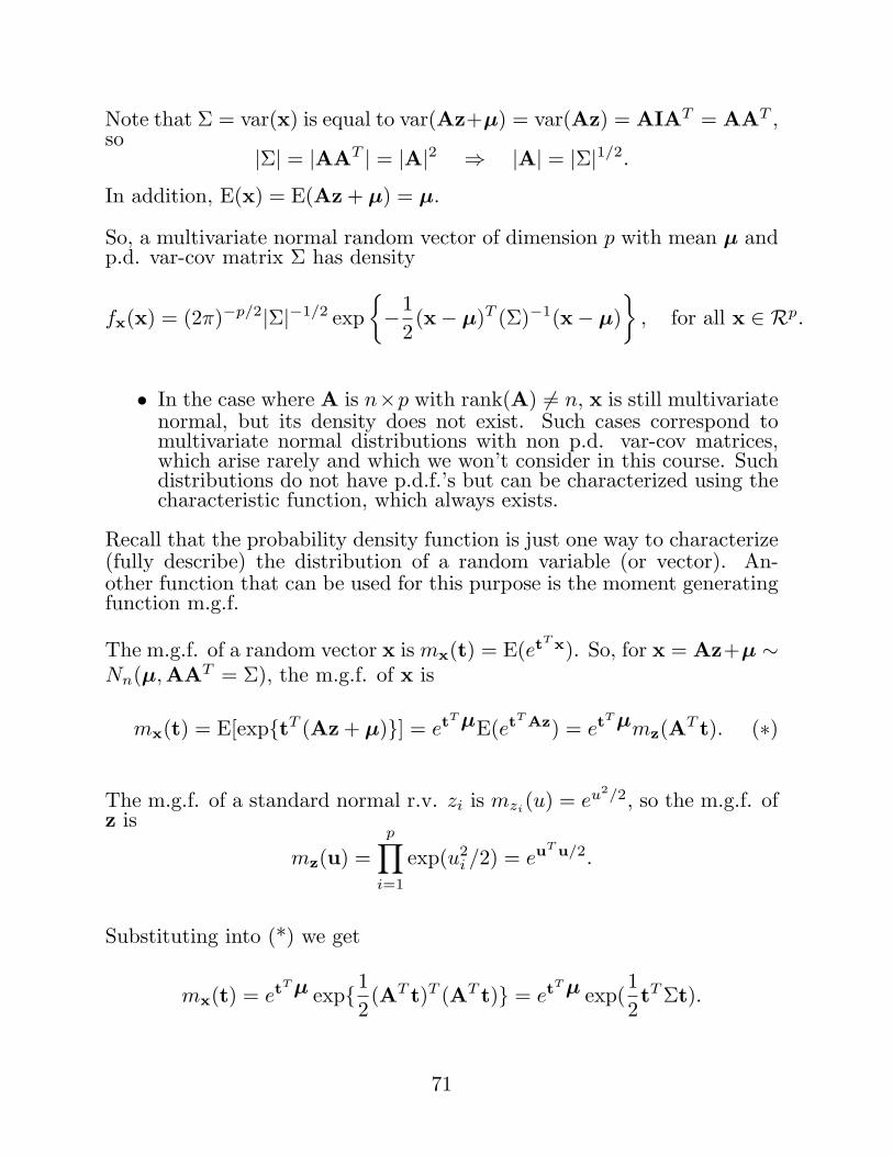
Note that Σ = var(x) is equal to var(Az+µ) = var(Az) = AIAT = AAT ,so

|Σ| = |AAT | = |A|2 ⇒ |A| = |Σ|1/2.

In addition, E(x) = E(Az + µ) = µ.

So, a multivariate normal random vector of dimension p with mean µ andp.d. var-cov matrix Σ has density

fx(x) = (2π)−p/2|Σ|−1/2 exp{−1

2(x− µ)T (Σ)−1(x− µ)

}, for all x ∈ Rp.

• In the case where A is n×p with rank(A) 6= n, x is still multivariatenormal, but its density does not exist. Such cases correspond tomultivariate normal distributions with non p.d. var-cov matrices,which arise rarely and which we won’t consider in this course. Suchdistributions do not have p.d.f.’s but can be characterized using thecharacteristic function, which always exists.

Recall that the probability density function is just one way to characterize(fully describe) the distribution of a random variable (or vector). An-other function that can be used for this purpose is the moment generatingfunction m.g.f.

The m.g.f. of a random vector x is mx(t) = E(etT x). So, for x = Az+µ ∼Nn(µ,AAT = Σ), the m.g.f. of x is

mx(t) = E[exp{tT (Az + µ)}] = etT µE(etT Az) = etT µmz(AT t). (∗)

The m.g.f. of a standard normal r.v. zi is mzi(u) = eu2/2, so the m.g.f. ofz is

mz(u) =p∏

i=1

exp(u2i /2) = euT u/2.

Substituting into (*) we get

mx(t) = etT µ exp{12(AT t)T (AT t)} = etT µ exp(

12tT Σt).

71

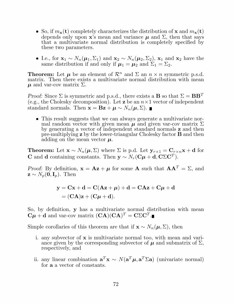
• So, if mx(t) completely characterizes the distribution of x and mx(t)depends only upon x’s mean and variance µ and Σ, then that saysthat a multivariate normal distribution is completely specified bythese two parameters.

• I.e., for x1 ∼ Nn(µ1, Σ1) and x2 ∼ Nn(µ2, Σ2), x1 and x2 have thesame distribution if and only if µ1 = µ2 and Σ1 = Σ2.

Theorem: Let µ be an element of Rn and Σ an n × n symmetric p.s.d.matrix. Then there exists a multivariate normal distribution with meanµ and var-cov matrix Σ.

Proof: Since Σ is symmetric and p.s.d., there exists a B so that Σ = BBT

(e.g., the Cholesky decomposition). Let z be an n×1 vector of independentstandard normals. Then x = Bz + µ ∼ Nn(µ,Σ).

• This result suggests that we can always generate a multivariate nor-mal random vector with given mean µ and given var-cov matrix Σby generating a vector of independent standard normals z and thenpre-multiplying z by the lower-triangular Cholesky factor B and thenadding on the mean vector µ.

Theorem: Let x ∼ Nn(µ,Σ) where Σ is p.d. Let yr×1 = Cr×nx + d forC and d containing constants. Then y ∼ Nr(Cµ + d,CΣCT ).

Proof: By definition, x = Az + µ for some A such that AAT = Σ, andz ∼ Np(0, Ip). Then

y = Cx + d = C(Az + µ) + d = CAz + Cµ + d

= (CA)z + (Cµ + d).

So, by definition, y has a multivariate normal distribution with meanCµ + d and var-cov matrix (CA)(CA)T = CΣCT .

Simple corollaries of this theorem are that if x ∼ Nn(µ,Σ), then

i. any subvector of x is multivariate normal too, with mean and vari-ance given by the corresponding subvector of µ and submatrix of Σ,respectively, and

ii. any linear combination aT x ∼ N(aT µ,aT Σa) (univariate normal)for a a vector of constants.

72

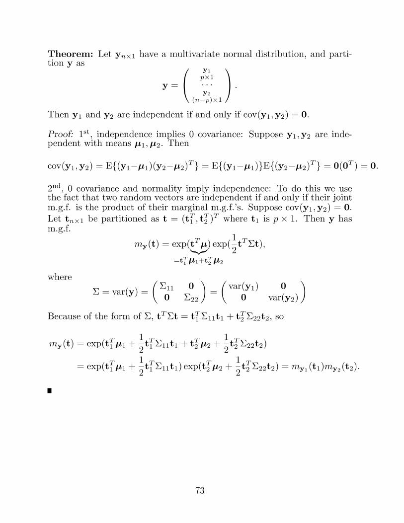
Theorem: Let yn×1 have a multivariate normal distribution, and parti-tion y as

y =

y1p×1· · ·y2

(n−p)×1

.

Then y1 and y2 are independent if and only if cov(y1,y2) = 0.

Proof: 1st, independence implies 0 covariance: Suppose y1,y2 are inde-pendent with means µ1, µ2. Then

cov(y1,y2) = E{(y1−µ1)(y2−µ2)T } = E{(y1−µ1)}E{(y2−µ2)T } = 0(0T ) = 0.

2nd, 0 covariance and normality imply independence: To do this we usethe fact that two random vectors are independent if and only if their jointm.g.f. is the product of their marginal m.g.f.’s. Suppose cov(y1,y2) = 0.Let tn×1 be partitioned as t = (tT

1 , tT2 )T where t1 is p × 1. Then y has

m.g.f.

my(t) = exp(tT µ︸︷︷︸=tT

1 µ1+tT2 µ2

) exp(12tT Σt),

where

Σ = var(y) =(

Σ11 00 Σ22

)=

(var(y1) 0

0 var(y2)

)

Because of the form of Σ, tT Σt = tT1 Σ11t1 + tT

2 Σ22t2, so

my(t) = exp(tT1 µ1 +

12tT1 Σ11t1 + tT

2 µ2 +12tT2 Σ22t2)

= exp(tT1 µ1 +

12tT1 Σ11t1) exp(tT

2 µ2 +12tT2 Σ22t2) = my1(t1)my2(t2).

73

Lemma: Let y ∼ Nn(µ, Σ) where we have the partitioning

y =

y1p×1· · ·y2

(n−p)×1

, µ =

(µ1

µ2

),Σ =

(Σ11 Σ12

Σ21 Σ22

),

where Σ21 = ΣT12. Let y2|1 = y2 − Σ21Σ−1

11 y1. Then y1 and y2|1 areindependent with

y1 ∼ Np(µ1, Σ11), y2|1 ∼ Nn−p(µ2|1,Σ22|1),

where

µ2|1 = µ2 − Σ21Σ−111 µ1, and Σ22|1 = Σ22 − Σ21Σ−1

11 Σ12.

Proof: We can write y1 = C1y where C1 = (I,0) and we can write y2|1 =C2y where C2 = (−Σ21Σ−1

11 , I), so by the theorem on the bottom of p.72, both y1 and y2|1 are normal. Their mean and variance-covariances areC1µ = µ1 and C1ΣCT

1 = Σ11 for y1, and C2µ = µ2|1 and C2ΣCT2 = Σ22|1

for y2|1. Independence follows from the fact that these two random vectorshave covariance matrix cov(y1,y2|1) = cov(C1y,C2y) = C1ΣCT

2 = 0.

Theorem: For y defined as in the previous theorem, the conditionaldistribution of y2 given y1 is

y2|y1 ∼ Nn−p(µ2 + Σ21Σ−111 (y1 − µ1), Σ22|1).

Proof: Since y2|1 is independent of y1, its conditional distribution for agiven value of y1 is the same as its marginal distribution, y2|1 ∼ Nn−p(µ2|1, Σ22|1).Notice that y2 = y2|1 + Σ21Σ−1

11 y1. Conditional on the value of y1,Σ21Σ−1

11 y1 is constant, so the conditional distribution of y2 is that of y2|1plus a constant, or (n− p)−variate normal, with mean

µ2|1 +Σ21Σ−111 y1 = µ2−Σ21Σ−1

11 µ1 +Σ21Σ−111 y1 = µ2 +Σ21Σ−1

11 (y1−µ1),

and var-cov matrix Σ22|1.

74

Partial and Multiple Correlation

Example — Height and Reading Ability:

Suppose that an educational psychologist studied the relationship betweenheight y1 and reading ability y2 of children based on scores on a standard-ized test. For 200 children in grades 3, 4, and 5 he measured y1 and y2and found that the sample correlation between these variables was .56.

Is there a linear association between height and reading ability?

Well, yes, but only because we’ve ignored one or more “lurking” variables.There is likely no direct effect of height on reading ability. Instead, olderchildren with more years of schooling tend to be better readers and tendto be taller. The effects of age on both y1 and y2 have been ignored byjust examining the simple correlation between y1 and y2.

The partial correlation coefficient is a measure of linear relationship be-tween two variables, with the linear effects of one or more other variables(in this case, age) removed.

75

Partial Correlation: Suppose v ∼ Np+q(µ, Σ) and let v, µ and Σ bepartitioned as

v =(

xy

), µ =

(µx

µy

), Σ =

(Σxx Σxy

Σyx Σyy

),

where x = (v1, . . . , vp)T is p× 1 and y = (vp+1, . . . , vp+q)T is q × 1.

Recall that the conditional var-cov matrix of y given x is

var(y|x) = Σyy − ΣyxΣ−1xxΣxy ≡ Σy|x.

Let σij|1,...,p denote the (i, j)th element of Σy|x.

Then the partial correlation coefficient of yi and yj given x = c isdefined by

ρij|1,...,p =σij|1,...,p

[σii|1,...,pσjj|1,...,p]1/2

(provided the denominator is non-zero, in which case ρij|1,...,p is unde-fined).

• Like the ordinary correlation coefficient, the partial correlation sat-isfies

−1 ≤ ρij|1,...,p ≤ 1.

• Interpretation: the partial correlation ρij|1,...,p measures the linearassociation between yi and yj after accounting for (or removing) thelinear association between yi and x and between yj and x.

– E.g., if v1 = age, v2 =height, v3 =reading ability, x = v1 andy = (v2, v3)T , then ρ23|1 = the correlation between height andreading ability after removing the effects of age on each of thesevariables. I would expect ρ23|1 ≈ 0.

76

The partial correlation measures the linear association between two vari-ables after removing the effects of several others. The multiple correla-tion coefficient measures the linear association between one variable anda group of several others.

Multiple Correlation: Suppose v ∼ Np+1(µ, Σ) and let v, µ and Σ bepartitioned as

v =(

xy

), µ =

(µx

µy

), Σ =

(Σxx σxy

σyx σyy

),

where x = (v1, . . . , vp)T is p×1, and y = vp+1 is a scalar random variable.

Recall that the conditional mean of y given x is

µy + σyxΣ−1xx (x− µx) ≡ µy|x.

Then the squared multiple correlation coefficient between y and xis defined as

ρ2y,x =

cov(µy|x, y)[var(µy|x)var(y)]1/2

.

• A computationally simple formula is given by

ρ2y,x =

{σyxΣ−1

xxσxy

σyy

}1/2

.

• My notation for this quantity is ρ2y,x rather than ρy,x because it

behaves like the square of a correlation coefficient. It is boundedbetween zero and one:

0 ≤ ρ2y,x ≤ 1,

and quantifies the strength of the linear association, but not thedirection.

• The sample squared multiple correlation coefficient is called the co-efficient of determination and usually denoted R2.

• We’ll talk about sample versions of the partial and multiple correla-tion coefficients later, when we get to fitting linear models.

77

Distributions of Quadratic Forms: The χ2, F , and t Distributions

• All three of these distributions arise as the distributions of certainfunctions of normally distributed random variables.

• Their central (ordinary) versions are probably familiar as the dis-tributions of normal-theory test statistics under the usual null hy-potheses and as the basis for confidence intervals.

• The non-central versions of these distributions arise as the distribu-tions of normal-theory test statistics under the alternatives to theusual null hypotheses. Thus, they are important in, for example,determining the power of tests.

Chi-square Distribution: Let x1, . . . , xn be independent normal ran-dom variables with means µ1, . . . , µn and common variance 1. Then

y = x21 + · · ·+ x2

n = xT x = ‖x‖2, where x = (x1, . . . , xn)T

is said to have a noncentral chi-square distribution with n degreesof freedom and noncentrality parameter λ = 1

2

∑ni=1 µ2

i . We denotethis as y ∼ χ2(n, λ).

• As in the t and F distributions, the central chi-square distributionoccurs when the noncentrality parameter λ equals 0.

• The central χ2 with n degrees of freedom will typically be denotedχ2(n) ≡ χ2(n, 0).

– In particular, for z1, . . . , zniid∼ N(0, 1), z2

1 + · · ·+ z2n ∼ χ2(n).

• The non-central χ2(n, λ) distribution depends only on its parame-ters, n and λ.

78

A random variable Y ∼ χ2(n) (a central χ2 with n d.f.) has p.d.f.

fY (y; n) =yn/2−1e−y/2

Γ(n/2)2n/2, for y > 0.

• This is a special case of a gamma density with power parameter n/2and scale parametr 1/2.

The non-central χ2 density is a Poisson mixture of central χ2’s. If Z ∼χ2(n, λ) then Z has p.d.f.

fZ(z; n, λ) =∞∑

k=0

p(k; λ)fY (z;n + 2k), for z > 0,

where p(k; λ) = {e−λ(λ)k}/k! is the Poisson probability function with rate(mean) λ.

• I.e., the noncentral χ2 is a weighted sum of central χ2’s with Poissonweights.

Theorem: Let Y ∼ χ2(n, λ). Then

i. E(Y ) = n + 2λ;ii. var(Y ) = 2n + 8λ; andiii. the m.g.f. of Y is

mY (t) =exp[−λ{1− 1/(1− 2t)}]

(1− 2t)n/2.

Proof: The proof of (i) and (ii) we leave as a homework problem. The proofof (iii) simply involves using the definition of expectation to evaluate

mY (t) = E(etY ) = E{et(xT x)} =∫ ∞

−∞· · ·

∫ ∞

−∞et(xT x) fx(x)︸ ︷︷ ︸a N(µ, I) density

dx1 . . . dxn,

where x is an n × 1 vector of independent normals with mean µ andconstant variance 1. See Graybill (1976, p. 126) for details.

79

The χ2 distribution has the convenient property that sums of independentχ2’s are χ2 too:

Theorem: If v1, . . . , vk are independent random variables distributed asχ2(ni, λi), i = 1, . . . , k, respectively, then

k∑

i=1

vi ∼ χ2(k∑

i=1

ni,k∑

i=1

λi).

Proof: follows easily from the definition.

Distribution of a Quadratic Form:

From the definition of a central chi-square, it is immediate that if y ∼Nn(µ, In) then

‖y − µ‖2 = (y − µ)T (y − µ) ∼ χ2(n).

For y ∼ Nn(µ, Σ) where Σ is p.d., we can extend this to

(y − µ)T Σ−1(y − µ) ∼ χ2(n)

by noting that

(y − µ)T Σ−1(y − µ) = (y − µ)T Σ−1/2Σ−1/2(y − µ)

= {Σ−1/2(y − µ)}T {Σ−1/2(y − µ)}︸ ︷︷ ︸≡z

= zT z,

where Σ−1/2 = (Σ1/2)−1, and Σ1/2 is the unique symmetric square rootof Σ (see p. 51 of these notes). Since z = Σ−1/2(y − µ) ∼ Nn(0, In), wehave that zT z = (y − µ)T Σ−1(y − µ) ∼ χ2(n).

80

We’d like to generalize these results on the distribution of quadratic formsto obtain the the distribution of yT Ay for y ∼ Nn(µ,Σ) for A a matrixof constants. We can do this, but first we need a couple of results.

Theorem: If y ∼ Nn(µ, Σ) then the m.g.f. of yT Ay is

myT Ay(t) = |In − 2tAΣ|−1/2 exp[−1

2µT {In − (In − 2tAΣ)−1}Σ−1µ

].

Proof: Again, the proof of this result “simply” involves evaluating theexpectation,

E(etyT Ay) =∫ ∞

−∞· · ·

∫ ∞

−∞etyT Ay fy(y)︸ ︷︷ ︸

a multi’normal density

dy1 . . . dyn.

See Searle, 1971, p.55, for details.

We also need a couple of eigenvalue results that we probably should havestated earlier:

Result: If λ is an eigenvalue of A and x is the corresponding eigenvectorof A, then for scalars c and k, (cλ+ k,x) is an eigenvalue-eigenvector pairof the matrix cA + kI.

Proof: Because (λ,x) is an eigen-pair for A, they satisfy Ax = λx whichimplies

cAx = cλx.

Adding kx to both sides of this equation we have

cAx + kx = cλx + kx

⇒ (cA + kI)x = (cλ + k)x,

so that (cλ+ k,x) is an eigenvalue-eigenvector pair of the matrix cA+ kI.

81

Result: If all of the eigenvalues of A satisfy −1 < λ < 1, then

(I−A)−1 = I + A + A2 + A3 + · · · = I +∞∑

k=1

Ak. (∗)

Proof: This can be verified by multiplying I−A times (I +∑∞

k=1 Ak) toobtain the identity matrix. Note that −1 < λ < 1 for all eigenvalues of Aensures limk→∞Ak → 0 so that

∑∞k=1 Ak converges.

Previously, we established that a projection matrix PV onto a subspaceV ∈ Rn where dim(V ) = k has k eigenvalues equal to 1, and n − keigenvalues equal to 0.

Recall that a projection matrix is symmetric and idempotent. More gen-erally, this result can be extended to all idempotent matrices.

Theorem: If A is an n × n idempotent matrix of rank r, then A has reigenvalues equal to 1, and n− r eigenvalues equal to 0.

Proof: In general, if λ is an eigenvalue for A, then λ2 is an eigenvalue forA2 since

A2x = A(Ax) = Aλx = λAx = λλx = λ2x.

Since A2 = A, we have A2x = Ax = λx. Equating the right sides ofA2x = λ2x and A2x = λx, we have

λx = λ2x, or (λ− λ2)x = 0.

But x 6= 0, so λ − λ2 = 0, from which λ must be either 0 or 1. Since Ais idempotent, it must be p.s.d., so the number of nonzero eigenvalues isequal to rank(A) = r and therefore, r eigenvalues are 1 and n− r are 0.

Now we are ready to state our main result:

Theorem: Let y ∼ Nn(µ,Σ) and A be a n × n symmetric matrix ofconstants with rank(A) = r. Let λ = 1

2µT Aµ. Then

yT Ay ∼ χ2(r, λ) if and only if AΣ is idempotent.

82

Proof: From the theorem on p. 81, the moment generating function ofyT Ay is

myT Ay(t) = |In − 2tAΣ|−1/2 exp[−1

2µT {In − (In − 2tAΣ)−1}Σ−1µ

].

By the result on p. 81, the eigenvalues of In − 2tAΣ are 1 − 2tλi, i =1, . . . , n, where λi is an eigenvalue of AΣ. Since the determinant equalsthe product of the eigenvalues, we have |In − 2tAΣ| = ∏n

i=1(1− 2tλi). Inaddition, by (*) we have (In−2tAΣ)−1 = In +

∑∞k=1(2t)k(AΣ)k provided

that −1 < 2tλi < 1 for all i. Thus myT Ay(t) can be written as

myT Ay(t) =

(n∏

i=1

(1− 2tλi)−1/2

)exp

[−1

2µT {−

∞∑

k=1

(2t)k(AΣ)k}Σ−1µ

].

Now suppose AΣ is idempotent of rank r = rank(A). Then (AΣ)k = AΣand r of the λi’s are equal to 1, and n − r of the λi’s are equal to 0.Therefore,

myT Ay(t) =

(r∏

i=1

(1− 2t)−1/2

)exp[−1

2µT {−

∞∑

k=1

(2t)k}AΣΣ−1µ]

= (1− 2t)−r/2 exp[−12µT {1− (1− 2t)−1}Aµ],

provided that −1 < 2t < 1 or − 12 < t < 1

2 , which is compatible with therequirement that the m.g.f. exist for t in a neighborhood of 0. (Here wehave used the series expansion 1/(1− x) = 1 +

∑∞k=1 xk for −1 < x < 1.)

Thus,

myT Ay(t) =exp[− 1

2µT Aµ{1− 1/(1− 2t)}](1− 2t)r/2

,

which is the m.g.f. of a χ2(r, 12µT Aµ) random variable.

For a proof of the converse (that yT Ay ∼ χ2(r, λ) implies AΣ idempo-tent), see Searle (1971, pp. 57–58).

83

Several useful results follow easily from the previous theorem as corollaries:

Corollary 1: If y ∼ Nn(0, σ2I), then 1σ2 yT Ay ∼ χ2(r) if and only if A

is idempotent of rank r.

Corollary 2: If y ∼ Nn(µ, σ2I), then 1σ2 yT Ay ∼ χ2(r, 1

2σ2 µT Aµ) if andonly if A is idempotent of rank r.

Corollary 3: Suppose y ∼ Nn(µ, σ2In) and let PV be the projectionmatrix onto a subspace V ∈ Rn of dimension r ≤ n. Then

1σ2

yT PV y =1σ2‖p(y|V )‖2 ∼ χ2(r,

12σ2

µT PV µ) = χ2(r,1

2σ2‖p(µ|V )‖2).

Corollary 4: Suppose y ∼ N(µ, Σ) and let c be an n × 1 vector ofconstants. Then

(y − c)T Σ−1(y − c) ∼ χ2(n, λ) for λ =12(µ− c)T Σ−1(µ− c).

The classical linear model has the form y ∼ Nn(µ, σ2In), where µ isassumed to lie in a subspace V = L(x1, . . . ,xk) = C(X). That is, µ = Xβfor some β ∈ Rk.

Therefore, we’ll be interested in statistical properties of yV = p(y|V ), theprojection of y onto V , and of functions of yV and the residual vectory − yV = p(y|V ⊥).

• The distributional form (normal, chi-square, etc.) of functions of y(e.g., yV ) are determined by the distributional form of y (usuallyassumed normal).

• The expectation of linear functions of y is determined solely byE(y) = µ.

• The expectation of quadratic functions of y (e.g., ‖yV ‖2) is deter-mined by µ and var(y).

84

In particular, we have the following results

Theorem: Let V be a k−dimensional subspace of Rn, and let y be arandom vector in Rn with mean E(y) = µ. Then

1. E{p(y|V )} = p(µ|V );

2. if var(y) = σ2In then

var{p(y|V )} = σ2PV and E{‖p(y|V )‖2} = σ2k + ‖p(µ|V )‖2;

and

3. if we assume additionally that y is m’variate normal i.e., y ∼ Nn(µ, σ2In),then

p(y|V ) ∼ Nn(p(µ|V ), σ2PV ),

and

1σ2‖p(y|V )‖2 =

1σ2

yT PV y ∼ χ2(k,1

2σ2µT PV µ︸ ︷︷ ︸

=‖p(µ|V )‖2).

Proof:

1. Since the projection operation is linear, E{p(y|V )} = p(E(y)|V ) =p(µ|V ).

2. p(y|V ) = PV y so var{p(y|V )} = var(PV y) = PV σ2InPTV = σ2PV .

In addition, ‖p(y|V )‖2 = p(y|V )T p(y|V ) = (PV y)T PV y = yT PV y.So, E(‖p(y|V )‖2) = E(yT PV y) is the expectation of a quadraticform and therefore equals

E(‖p(y|V )‖2) = tr(σ2PV ) + µT PV µ = σ2tr(PV ) + µT PTV PV µ

= σ2k + ‖p(µ|V )‖2.

3. Result 3 is just a restatement of corollary 3 above, and follows im-mediately from the Theorem on the bottom of p. 82.

85

So, we have distributional results for a projection and for the squaredlength of that projection. In linear models we typically decompose thesample space by projecting onto the model space V to form yV = p(y|V )and onto its orthogonal complement V ⊥ to form the residual e = y− yV .In some cases we go further and decompose the model space by projectingonto subspaces within the model space.

What’s the joint distribution of such projections?

Well, it turns out that if the subspaces are orthogonal and if the conditionsof the classical linear model (normality, independence, and homoscedas-ticity) hold, then the projections onto these subspaces are independentnormal random vectors, and their squared lengths (the sums of squares inan ANOVA) are independent chi-square random variables.

So, if we understand the geometry underlying our linear model (e.g., un-derlying an ANOVA we’d like to do for a particular linear model), thenwe can use the following result:

Theorem: Let V1, . . . , Vk be mutually orthogonal subspaces of Rn withdimensions d1, . . . , dk, respectively, and let y be a random vector takingvalues in Rn which has mean E(y) = µ. Let Pi be the projection matrixonto Vi so that yi = p(y|Vi) = Piy and let µi = Piµ, i = 1, . . . , n. Then

1. if var(y) = σ2In then cov(yi, yj) = 0, for i 6= j; and

2. if y ∼ Nn(µ, σ2In) then y1, . . . , yk are independent, with

yi ∼ N(µi, σ2Pi);

and

3. if y ∼ Nn(µ, σ2In) then ‖y1‖2, . . . , ‖yk‖2 are independent, with

1σ2‖yi‖2 ∼ χ2(di,

12σ2

‖µi‖2).

86

Proof: Part 1: For i 6= j, cov(yi, yj) = cov(Piy,Pjy) = Picov(y,y)Pj =Piσ

2IPj = σ2PiPj = 0. (For any z ∈ Rn, PiPjz = 0 ⇒ PiPj = 0.)

Part 2: If y is m’variate normal then yi = Piy, i = 1, . . . , k, are jointlymultivariate normal and are therefore independent if and only if cov(yi, yj) =0, i 6= j. The mean and variance-covariance of yi are E(yi) = E(Piy) =Piµ = µi and var(yi) = Piσ

2IPTi = σ2Pi.

Part 3: If yi = Piy, i = 1, . . . , k, are mutually independent, then any(measurable*) functions fi(yi), i = 1, . . . , k, are mutually independent.Thus ‖yi‖2, i = 1, . . . , k, are mutually independent. That σ−2‖yi‖2 ∼χ2(di,

12σ2 ‖µi‖2) follows from part 3 of the previous theorem.

Alternatively, we can take an algebraic approach to determining whetherprojections and their squared lengths (in, for example, an ANOVA) areindependent. The geometric approach is easier, perhaps, but only if youunderstand the geometry. But we will describe the algebraic approach aswell (next).

Independence of Linear and Quadratic Forms:

Here we consider the statistical independence of:

1. a linear form and a quadratic form (e.g., consider whether y and s2 ina one sample problem are independent; or consider the independenceof β and s2 in a regression setting);

2. two quadratic forms (e.g., consider the independence of the sum ofsquares due to regression and the error sum of squares in a regressionproblem); and

3. several quadratic forms (e.g., consider the joint distribution of SSA,SSB , SSAB , SSE in a two-way layout analysis of variance).

* All continuous functions, and most “well-behaved” functions aremeasurable

87

Before proceeding, we need a Lemma and its corollary:

Lemma: If y ∼ Nn(µ,Σ), then

cov(y,yT Ay) = 2ΣAµ.

Proof: Using the definition of covariance and the expectation of a quadraticform, we have

cov(y,yT Ay) = E[(y − µ){yT Ay − E(yT Ay)}]= E[(y − µ){yT Ay − tr(AΣ)− µT Aµ}].

Now using the algebraic identity yT Ay − µT Aµ = (y − µ)T A(y − µ) +2(y − µ)T Aµ, we obtain

cov(y,yT Ay) = E[(y − µ){(y − µ)T A(y − µ) + 2(y − µ)T Aµ− tr(AΣ)}]= E{(y − µ)(y − µ)T A(y − µ)}+ 2E{(y − µ)(y − µ)T Aµ}− E{(y − µ)tr(AΣ)}

= 0 + 2ΣAµ− 0.

The first term equals 0 here because all third central moments of themultivariate normal distribution are 0.

Corollary: Let B be a k×n matrix of constants and y ∼ Nn(µ, Σ). Then

cov(By,yT Ay) = 2BΣAµ.

Now we are ready to consider (1.):

Theorem: Suppose B is a k × n matrix of constants, A a n × n sym-metric matrix of constants, and y ∼ Nn(µ,Σ). Then By and yT Ay areindependent if and only if BΣA = 0k×n.

Proof: We prove this theorem under the additional assumption that A isa projection matrix (that is, assuming A is idempotent as well as symmet-ric), which is the situation in which we’re most interested in this course.See Searle (1971, p.59) for the complete proof.

88

Assuming A is symmetric and idempotent, then we have

yT Ay = yT AT Ay = ‖Ay‖2.

Now suppose BΣA = 0. Then By and Ay are each normal, with

cov(By,Ay) = BΣA = 0.

Therefore, By and Ay are independent of one another. Furthermore,By is independent of any (measureable) function of Ay, so that By isindependent of ‖Ay‖2 = yT Ay.Now for the converse. Suppose By and yT Ay are independent. Thencov(By,yT Ay) = 0 so

0 = cov(By,yT Ay) = 2BΣAµ,

by the corollary to the lemma above. Since this holds for all possible µ, itfollows that BΣA = 0.

Corollary: If y ∼ Nn(µ, σ2I), then By and yT Ay are independent ifand only if BA = 0.

Example: Suppose we have a random sample y = (y1, . . . , yn)T ∼ Nn(µ, σ2In),and consider

y =1n

n∑

i=1

yi =1njTny

and

s2 =1

n− 1

n∑

i=1

(yi − y)2 =1

n− 1‖PL(jn)⊥y‖2

where PL(jn)⊥ = In − 1n jnjTn . By the above corollary, y and s2 are inde-

pendent because

1njTnPL(jn)⊥ =

1n

(PTL(jn)⊥jn)T = (PL(jn)⊥jn)T =

1n

(0)T = 0T .

89

Theorem: Let A and B be symmetric matrices of constants. If y ∼Nn(µ,Σ), then yT Ay and yT By are independent if and only if AΣB = 0.

Proof: Again, we consider the special case when A and B are symmetricand idempotent (projection matrices), and we only present the “if” partof the proof (see Searle, 1971, pp. 59–60, for complete proof).

Suppose A and B are symmetric and idempotent and that AΣB = 0.Then yT Ay = ‖Ay‖2, yT By = ‖By‖2. If AΣB = 0 then

cov(Ay,By) = AΣB = 0.

Each of Ay and By are multivariate normal and they have covariance 0,hence they’re independent. Furthermore, any (measurable) functions ofAy and By are independent, so that ‖Ay‖2 and ‖By‖2 are independent.

Corollary: If y ∼ Nn(µ, σ2I) then yT Ay and yT By are independent ifand only if AB = 0.

Finally, we have a theorem and corollary concerning the mutual indepen-dence of several quadratic forms in normal random vectors:

Theorem: Let y ∼ Nn(µ, σ2In), let Ai be symmetric of rank ri, i =1, . . . , k, and let A =

∑ki=1 Ai with rank r so that yT Ay =

∑ki=1 yT Aiy.

Then

1. yT Aiy/σ2 ∼ χ2(ri, µT Aiµ/{2σ2}), i = 1, . . . , k; and

2. yT Aiy and yT Ajy are independent for all i 6= j; and3. yT Ay/σ2 ∼ χ2(r,µT Aµ/{2σ2});

if and only if any two of the following statements are true:

a. each Ai is idempotent;b. AiAj = 0 for all i 6= j;c. A is idempotent;

or if and only if (c) and (d) are true where (d) is as follows:

d. r =∑k

i=1 ri.

90

Proof: See Searle (1971, pp. 61–64).

• Note that any two of (a), (b), and (c) implies the third.

• The previous theorem concerned the partitioning of a weighted sumof squares yT Ay into several components. We now state a corollarythat treats the special case where A = I and the total (unweightedsum of squares) yT y is decomposed into a sum of quadratic forms.

Corollary: Let y ∼ Nn(µ, σ2I), let Ai be symmetric of rank ri, i =1, . . . , k, and suppose that yT y =

∑ki=1 yT Aiy (i.e.,

∑ki=1 Ai = I). Then

1. each yT Aiy ∼ χ2(ri, µT Aiµ/{2σ2}); and

2. the yT Aiy’s are mutually independent;

if and only if any one of the following statements holds:

a. each Ai is idempotent;b. AiAj = 0 for all i 6= j;c. n =

∑ki=1 ri.

• This theorem subsumes “Cochran’s Theorem” which is often citedas the justification for independence of sums of squares in a decom-position of the total sum of squares in an analysis of variance.

91

F -Distribution: Let

U1 ∼ χ2(n1, λ), U2 ∼ χ2(n2) (central)

be independent. Then

V =U1/n1

U2/n2

is said to have a noncentral F distribution with noncentrality parameterλ, and n1 and n2 degrees of freedom.

• For λ = 0, V is said to have a central F distribution with degrees offreedom n1 and n2.

• The noncentral F has three parameters: λ, the noncentrality param-eter, n1, the numerator degrees of freedom, and n2, the denominatordegrees of freedom. The central F has two parameters, the numera-tor and denominator degrees of freedom, n1 and n2.

• We’ll denote the noncentral F by F (n1, n2, λ) and the central F byF (n1, n2). The 100γth percentile of the F (n1, n2) distribution willbe denoted Fγ(n1, n2).

• The p.d.f. of the noncentral F is an ugly looking thing not worthreproducing here. It has the form of a Poisson mixture of centralF ’s.

• The mean of the noncentral F (n1, n2, λ) is n2n2−2 (1 + 2λ/n1). Its

variance is much more complicated (see Stapleton, p.67, if you’reinterested).

92

t-Distribution: Let

W ∼ N(µ, 1), Y ∼ χ2(m)

be independent random variables. Then

T =W√Y/m

is said to have a (Student’s) t distribution with noncentrality parameterµ and m degrees of freedom.

• We’ll denote this distribution as t(m,µ).

• If the numerator random variable W has distribution N(µ, σ2) thenthe noncentrality parameter becomes µ/σ since W/σ ∼ (µ/σ, 1).

• Again, when the noncentrality parameter µ is zero, we get the centralt distribution, t(m) ≡ t(m, 0). The 100γth percentile of the central twill be denoted tγ(m).

• The p.d.f. of the noncentral t is too complicated to be worth becom-ing familiar with. It may be found in Stapleton, p.68.

• The mean and variance of the central t(m) distribution are 0, andm/(m − 2), respectively. For the noncentral t, these moments arenot so simple.

• We can think of the central t(m) has a more dispersed version ofthe standard normal distribution with fatter tails. As m → ∞,m/(m− 2) → 1, so the t(m) converges to the N(0, 1).

Notice the important relationship that the square of a r.v. with a t(m)distribution has an F (1,m) distribution:

IfT =

W√Y/m

∼ t(m),

then

T 2 =W 2/1Y/m

∼ F (1,m).

93

Example: Let Y1, . . . , Yn be a random sample from a N(µ, σ2) distribu-tion. The following results should be familiar to you from earlier course-work (we will prove them in the following theorem): For Y = 1

n

∑ni=1 Yi,

and S2 = 1n−1

∑ni=1(Yi − Y )2,

Y ∼ N

(µ,

σ2

n

),

(n− 1)S2

σ2∼ χ2(n− 1), and Y , S2 are independent.

Let µ0 be a constant, and define θ = µ−µ0σ/√

n. Then

T =Y − µ0

S/√

n∼

{t(n− 1), if µ0 = µ;t(n− 1, θ), otherwise.

Here’s the theorem establishing these results, and providing the basis forthe one-sample t−test.

Theorem: Let Y1, . . . , Yn be a random sample (i.i.d. r.v.’s) from aN(µ, σ2) distribution, and let Y , S2, and T be defined as above. Then

1. Y ∼ N(µ, σ2/n);

2. V = S2(n−1)σ2 = 1

σ2

∑ni=1(Yi − Y )2 ∼ χ2(n− 1);

3. Y and S2 are independent; and

4. T = Y−µ0S/√

n∼ t(n− 1, λ) where λ = µ−µ0

σ/√

nfor any constant µ0.

Proof: Part 1: By assumption, y = (Y1, . . . , Yn)T ∼ Nn(µjn, σ2In).Let V = L(jn), a 1-dimensional subspace of Rn. Then p(y|V ) = Y jn.Y = n−1jTny is an affine transformation of y so it is normal, with meann−1jTnE(y) = µ and variance n−2jTnσ2Injn = σ2/n.

94

Part 3: By part 2 of the theorem on p. 86, p(y|V ⊥) = (Y1−Y , . . . , Yn−Y )T

is independent of p(y|V ) = Y jn, and hence independent of Y . Thus, S2,a function of p(y|V ⊥), and Y are independent. Alternatively, we coulduse the corollary on p. 89 giving the necessary and sufficient conditionfor independence of a linear form (Y ) and a quadratic form (S2). See theexample on p. 89.

Part 2: Here we use part 3 of the theorem on p. 85. That result impliesthat 1

σ2 S2(n− 1) = 1σ2 ‖p(y|V ⊥)‖2 ∼ χ2(dim(V ⊥), λ) = χ2(n− 1, λ) and

λ =1

2σ2‖p(E(y)|V ⊥)‖2 =

12σ2

‖ p(µjn︸︷︷︸∈V

|V ⊥)

︸ ︷︷ ︸=0

‖2 = 0.

Part 4: Let U = Y−µ0σ/√

n. Then U ∼ N

(µ−µ0σ/√

n, 1

). From part 3 of this

theorem, U and V are independent. Note that T can be written as

T =Y − µ0

S/√

n=

Y−µ0σ/√

n√S2/σ2

=U√

V/(n− 1),

so by the definition of the noncentral t distribution, T ∼ t(n− 1, µ−µ0

σ/√

n

).

95

Finally, the following theorem puts together some of our results on in-dependence of squared lengths of projections (quadratic forms) and thedefinition of the F distribution to give the distribution of F -tests in theANOVA:

Theorem: Let y = Xβ + e, where X is n × k with rank r ≤ k. ande ∼ Nn(0, σ2In). Let V1 be a subspace of C(X) with dim(V1) = r1 whichis smaller than dim(C(X)) = r. Let y = p(y|C(X)). Then the randomvariable

F =‖p(y|V1)‖2/r1

‖y − y‖2/(n− r)∼ F (r1, n− r, ‖p(Xβ|V1)‖2/{2σ2}).

Proof: Since y − y = p(y|C(X)⊥), it follows from part 3 of the theoremon p. 86 that Q1 ≡ ‖p(y|V1)‖2 and Q2 ≡ ‖p(y|C(X)⊥)‖2 = ‖y − y‖2 areindependent random variables and Q1/σ2 ∼ χ2(r1, ‖p(Xβ|V1)‖2/{2σ2})and Q2/σ2 ∼ χ2(n − r). Thus, by the definition of the non-central Fdistribution, the result follows.

96

The Linear Model

The Full Rank Case: Multiple Linear Regression

Suppose that on a random sample of n units (patients, animals, trees, etc.)we observe a response variable Y and explanatory variables X1, . . . , Xk.

Our data are then (yi, xi1, . . . , xik), i = 1, . . . , n, or, in vector/matrix formy,x1, . . . ,xk where y = (y1, . . . , yn) and xj = (x1j , . . . , xnj)T ; or y,Xwhere X = (x1, . . . ,xk).

Either by design or by conditioning on their observed values, x1, . . . ,xk

are regarded as vectors of known constants.

The linear model in its classical form makes the following assumptions:

A1. (additive error) y = µ + e where e = (e1, . . . , en)T is an unobservedrandom vector with E(e) = 0. This implies that µ = E(y) is theunknown mean of y.

A2. (linearity) µ = β1x1+· · ·+βkxk = Xβ where β1, . . . , βk are unknownparameters. This assumption says that E(y) = µ ∈ L(x1, . . . ,xk) =C(X) lies in the column space of X; i.e., it is a linear combinationof explanatory vectors x1, . . . ,xk with coefficients the unknown pa-rameters in β = (β1, . . . , βk)T .

• Linear in β1, . . . , βk not in the x’s.

A3. (independence) e1, . . . , en are independent random variables (andtherefore so are y1, . . . , yn).

A4. (homoscedasticity) e1, . . . , en all have the same variance σ2; thatis, var(e1) = · · · = var(en) = σ2 which implies var(y1) = · · · =var(yn) = σ2.

A5. (normality) e ∼ Nn(0, σ2In).

97

• Taken together, assumptions (A3) and (A4) say var(y) = var(e) =σ2In. We say that y (and e) has a spherical variance-covariancematrix.

• Note that assumption (A5) subsumes (A3) and (A4), but we canobtain many useful results without invoking normality, so its usefulto separate the assumptions of independence, homoscedasticity, andnormality.

• Taken together, all five assumptions can be stated more succinctlyas y ∼ Nn(Xβ, σ2I).

• The unknown parameters of the model are β1, . . . , βk, σ2.

• In multiple linear regression models, there is typically an interceptterm in the model. That is, one of the explanatory variables is equalto 1, for all i.

• This could be accommodated by just setting x1 = jn and letting β1

represent the intercept. However, we’ll follow our book’s conventionand include the intercept as an additional term. Our model thenbecomes

yi = β0 + β1xi1 + β2xi2 + · · ·+ βkxik, i = 1, . . . , n,

or

y1

y2...

yn

=

1 x11 x12 · · · x1k

1 x21 x22 · · · x2k...

......

...1 xn1 xn2 · · · xnk

︸ ︷︷ ︸=X

β0

β1...

βk

︸ ︷︷ ︸=β

+

e1

e2...

en

ory = Xβ + e,

where e ∼ Nn(0, σ2I).

98

• In multiple regression, it is typical for the explanatory vectors jn,x1,x2, . . . ,xk to be LIN. At times this is violated, but usually because ofthe data we happen to observe rather than because of the structureof the model. That is, in contrast to ANOVA models, there is usuallyno structural dependence among the explanatory vectors in multipleregression. Therefore, we will (for now) assume that X is offull rank.

• Note that our model assumes that we can re-express E(y) = µ ∈ Rn

as Xβ ∈ C(X) where dim(C(X)) = k + 1. Therefore, as long asn > k + 1, our model involves some reduction or summarization byassuming that the n-element vector µ falls in a k + 1 dimensionalsubspace of Rn.

• We will assume n > k + 1 throughout our discussion of the linearmodel. If n = k + 1 (when there are as many parameters in β asthere are data points), then the model involves no data reductionat all, only a data transformation. A linear model with k + 1 > nparameters is useless.

Interpretation of the βj ’s: The elements of β in a multiple linear regres-sion model are usually called simply regression coefficients, but are moreproperly termed partial regression coefficients.

In the modely = β0 + β1x1 + β2x2 + · · ·+ βkxk︸ ︷︷ ︸

=µ

+e,

note that ∂µ∂xk

= βj . That is, βj represents the change in E(y) = µassociated with a unit change in xj , assuming all of the other xk’s areheld constant.

In addition, this effect depends upon what other explanatory variables arepresent in the model. For example, β0 and β1 in the model

y = β0jn + β1x1 + β2x2 + e

will typically be different than β∗0 and β∗1 in the model

y = β∗0 jn + β∗1x1 + e∗.

99

• For example, consider again our reading ability and height example.If I regressed reading ability (r) on height (h) for children from grades1–5,

ri = β0 + β1hi + ei i = 1, . . . , n,

I would expect to obtain a large positive (and significant) estimateβ1. However, if we were to add age (a) to our model:

ri = β∗0 + β∗1hi + β∗2ai + e∗i i = 1, . . . , n,

I would expect β∗1 ≈ 0.

• The issue here is very similar to the distinction between correlationand partial correlation. However, regression coefficients quantify as-sociation between a random y and a fixed xj . Correlation coefficientsregard both y and xj as random.

Estimation in the Full-Rank Linear Model

Recall in the classical linear model (CLM) we assume

y = µ + e, for µ = Xβ for some β ∈ Rk+1, and e ∼ Nn(0, σ2In).

• Sometimes we are interested only in estimating E(y) = µ (e.g., whenfocused on prediction).

• More often, however, the parameters β0, β1, . . . , βk, or some subsetor function of the parameters are of interest in and of themselves asinterpretable, meaningful quantities to be estimated. Therefore, wewill focus on estimation of β rather than µ.

• However, the relationship between the mean parameter µ and theregression parameter β is µ = Xβ, so we can always estimate µ oncewe estimate β as µ = Xβ.

• In addition, in the X of full rank case, we can write β in terms of µ:β = (XT X)−1XT µ, so we could just as well focus on estimation ofµ and then obtain β as (XT X)−1XT µ.

100

Least-Squares Estimation:

Recall that the projection of y onto C(X), the set of all vectors of theform Xb for b ∈ Rk+1, yields the closest point in C(X) to y. That is,p(y|C(X)) yields the minimizer of

Q(β) = ‖y −Xβ‖2 (the least squares criterion)

This leads to the estimator β given by the solution of

XT Xβ = XT y (the normal equations)

orβ = (XT X)−1XT y.

All of this has already been established back when we studied projections(see pp. 30–31). Alternatively, we could use calculus:

To find a stationary point (maximum, minimum, or saddle point) of Q(β),we set the partial derivative of Q(β) equal to zero and solve:

∂

∂βQ(β) =

∂

∂β(y −Xβ)T (y −Xβ) =

∂

∂β(yT y − 2yT Xβ + βT (XT X)β)

= 0− 2XT y + 2XT Xβ

Here we’ve used the vector differentiation formulas ∂∂zc

T z = c and ∂∂zz

T Az =2Az (see §2.14 of our text).

Setting this result equal to zero, we obtain the normal equations, whichhas solution β = (XT X)−1XT y. That this is a minimum rather thana max, or saddle point can be verified by checking the second derivativematrix of Q(β):

∂2Q(β)∂β

= 2XT X

which is positive definite (result 7, p. 54), therefore β is a minimum.

101

Example — Simple Linear Regression

Consider the case k = 1:

yi = β0 + β1xi + ei, i = 1, . . . , n

where e1, . . . , en are i.i.d. each with mean 0 and variance σ2. Then themodel equation becomes

y1

y2...

yn

=

1 x1

1 x2...

...1 xn

︸ ︷︷ ︸=X

(β0

β1

)

︸ ︷︷ ︸=β

+

e1

e2...

en

.

It follows that

XT X =(

n∑

i xi∑i xi

∑i x2

i

), XT y =

( ∑i yi∑

i xiyi

)

(XT X)−1 =1

n∑

i x2i − (

∑i xi)2

( ∑i x2

i −∑i xi

−∑i xi n

).

Therefore, β = (XT X)−1XT y yields

β =(

β0

β1

)=

1n

∑i x2

i − (∑

i xi)2

((∑

i x2i )(

∑i yi)− (

∑i xi)(

∑i xiyi)

−(∑

i xi)(∑

i yi) + n∑

i xiyi

).

After a bit of algebra, these estimators simplify to

β1 =∑

i(xi − x)(yi − y)∑i(xi − x)2

=Sxy

Sxx

and β0 = y − β1x

102

In the case that X is of full rank, β and µ are given by

β = (XT X)−1XT y, µ = Xβ = X(XT X)−1XT y = PC(X)y.

• Notice that both β and µ are linear functions of y. That is, in eachcase the estimator is given by some matrix times y.

Note also that

β = (XT X)−1XT y = (XT X)−1XT (Xβ + e) = β + (XT X)−1XT e.

From this representation several important properties of the least squaresestimator β follow easily:

1. (unbiasedness):

E(β) = E(β + (XT X)−1XT e) = β + (XT X)−1XT E(e)︸︷︷︸=0

= β.

2. (var-cov matrix)

var(β) = var(β + (XT X)−1XT e) = (XT X)−1XT var(e)︸ ︷︷ ︸=σ2I

X(XT X)−1

= σ2(XT X)−1

3. (normality) β ∼ Nk(β, σ2(XT X)−1) (if e is assumed normal).

• These three properties require increasingly strong assumptions. Prop-erty (1) holds under assumptions A1 and A2 (additive error andlinearity).

• Property (2) requires, in addition, the assumption of sphericity.

• Property (3) requires assumption A5 (normality). However, later wewill present a central limit theorem-like result that establishes theasymptotic normality of β under certain conditions even when e isnot normal.

103

Example — Simple Linear Regression (Continued)

Result 2 on the previous page says for var(y) = σ2I, var(β) = σ2(XT X)−1.Therefore, in the simple linear regression case,

var(

β0

β1

)= σ2(XT X)−1

=σ2

n∑

i x2i − (

∑i xi)2

( ∑i x2

i −∑i xi

−∑i xi n

)

=σ2

∑i(xi − x)2

(n−1

∑i x2

i −x−x 1

).

Thus,

var(β0) =σ2

∑i x2

i /n∑i(xi − x)2

= σ2

[1n

+x2

∑i(xi − x)2

],

var(β1) =σ2

∑i(xi − x)2

,

and cov(β0, β1) =−σ2x∑

i(xi − x)2

• Note that if x > 0, then cov(β0, β1) is negative, meaning that theslope and intercept are inversely related. That is, over repeatedsamples from the same model, the intercept will tend to decreasewhen the slope increases.

104

Gauss-Markov Theorem:

We have seen that in the spherical errors, full-rank linear model, the least-squares estimator β = (XT X)−1XT y is unbiased and it is a linear esti-mator.

The following theorem states that in the class of linear and unbiased esti-mators, the least-squares estimator is optimal (or best) in the sense thatit has minimum variance among all estimators in this class.

Gauss-Markov Theorem: Consider the linear model y = Xβ+e whereX is n × (k + 1) of rank k + 1, where n > k + 1, E(e) = 0, and var(e) =σ2I. The least-squares estimators βj , j = 0, 1, . . . , k (the elements ofβ = (XT X)−1XT y have minimum variance among all linear unbiasedestimators.

Proof: Write βj as βj = cT β where c is the indicator vector containing a 1in the (j +1)st position and 0’s elsewhere. Then βj = cT (XT X)−1XT y =aT y where a = X(XT X)−1c. The quantity being estimated is βj = cT β =cT (XT X)−1XT µ = aT µ where µ = Xβ.

Consider an arbitrary linear estimator βj = dT y of βj . For such an esti-mator to be unbiased, it must satisfy E(βj) = E(dT y) = dT µ = aT µ forany µ ∈ C(X). I.e.,

dT µ− aT µ = 0 ⇒ (d− a)T µ = 0 for all µ ∈ C(X),

or (d− a) ⊥ C(X). Then

βj = dT y = aT y + (d− a)T y = βj + (d− a)T y.

The random variables on the right-hand side, βj and (d − a)T y, havecovariance

cov(aT y, (d− a)T y) = aT var(y)(d− a) = σ2aT (d− a) = σ2(dT a− aT a).

Since dT µ = aT µ for any µ ∈ C(X) and a = X(XT X)−1c ∈ C(X), itfollows that dT a = aT a so that

cov(aT y, (d− a)T y) = σ2(dT a− aT a) = σ2(aT a− aT a) = 0.

105

It follows that

var(βj) = var(βj) + var((d− a)T y) = var(βj) + σ2||d− a||2.

Therefore, var(βj) ≥ var(βj) with equality if and only if d = a, or equiva-lently, if and only if βj = βj .

Comments:

1. Notice that nowhere in this proof did we make use of the specificform of c as an indicator for one of the elements of β. That is,we have proved a slightly more general result than that given in thestatement of the theorem. We have proved that cT β is the minimumvariance estimator in the class of linear unbiased estimators of cT βfor any vector of constant c.

2. The least-squares estimator cT β where β = (XT X)−1XT y is oftencalled the B.L.U.E. (best linear unbiased estimator) of cT β. Some-times, it is called the Gauss-Markov estimator.

3. The variance of the BLUE is

var(cT β) = σ2‖a‖2 = σ2[X(XT X)−1c

]TX(XT X)−1c = σ2

[cT (XT X)−1c

].

Note that this variance formula depends upon X through (XT X)−1.Two implications of this observation are:

– If the columns of the X matrix are mutually orthogonal, then(XT X)−1 will be diagonal, so that the elements of β are un-correlated.

– Even for a given set of explanatory variables, the values atwhich the explanatory variable are observed will affect the vari-ance (precision) of the resulting parameter estimators.

4. What is remarkable about the Gauss-Markov Theorem is its distri-butional generality. It does not require normality! It says that β isBLUE regardless of the distribution of e (or y) as long as we havemean zero, spherical errors.

106

An additional property of least-squares estimation is that the estimatedmean µ = X(XT X)−1XT y is invariant to (doesn’t change as a result of)linear changes of scale in the explanatory variables.

That is, consider the linear models

y =

1 x11 x12 · · · x1k

1 x21 x22 · · · x2k...

......

. . ....

1 xn1 xn2 · · · xnk

︸ ︷︷ ︸=X

β + e

and

y =

1 c1x11 c2x12 · · · ckx1k

1 c1x21 c2x22 · · · ckx2k...

......

. . ....

1 c1xn1 c2xn2 · · · ckxnk

︸ ︷︷ ︸=Z

β∗ + e

Then, µ, the least squares estimator of E(y), is the same in both of thesetwo models. This follows from a more general theorem:

Theorem: In the linear model y = Xβ + e where E(e) = 0 and X is offull rank, µ, the least-squares estimator of E(y) is invariant to a full ranklinear transformation of X.

Proof: A full rank linear transformation of X is given by

Z = XH

where H is square and of full rank. In the original (untransformed) linearmodel µ = X(XT X)−1XT y = PC(X)y. In the transformed model y =Zβ∗+e, µ = Z(ZT Z)−1ZT y = PC(Z)y = PC(XH)y. So, it suffices to showthat PC(X) = PC(XH). This is true because if x ∈ C(XH) then x = XHbfor some b, ⇒ x = Xc where c = Hb ⇒ x ∈ C(X) ⇒ C(XH) ⊂ C(X).In addition, if x ∈ C(X) then x = Xd for some d ⇒ x = XHH−1d =XHa where a = H−1d ⇒ x ∈ C(XH) ⇒ C(X) ⊂ C(XH). Therefore,C(X) = C(XH).

• The simple case described above where each of the xj ’s is rescaledby a constant cj occurs when H = diag(1, c1, c2, . . . , ck).

107

Maximum Likelihood Estimation:

Least-squares provides a simple, intuitively reasonable criterion for esti-mation. If we want to estimate a parameter describing µ, the mean ofy, then choose the parameter value that minimizes the squared distancebetween y and µ. If var(y) = σ2I, then the resulting estimator is BLUE(optimal, in some sense).

• Least-squares is based only on assumptions concerning the mean andvariance-covaraince matrix (the first two moments) of y.

• Least-squares tells us how to estimate parameters associated withthe mean (e.g., β) but nothing about how to estimate parametersdescribing the variance (e.g., σ2) or other aspects of the distributionof y.

An alternative method of estimation is maximum likelihood estimation.

• Maximum likelihood requires the specification of the entire distribu-tion of y (up to some unknown parameters), rather than just themean and variance of that distribution.

• ML estimation provides a criterion of estimation for any parameterdescribing the distribution of y, including parameters describing themean (e.g., β), variance (σ2), or any other aspect of the distribution.

• Thus, ML estimation is simultaneously more general and less generalthan least squares in certain senses. It can provide estimators ofall sorts of parameters in a broad array of model types, includingmodels much more complex than those for which least-squares isappropriate; but it requires stronger assumptions than least-squares.

108

ML Estimation:

Suppose we have a discrete random variable Y (possibly a vector) withobserved value y. Suppose Y has probability mass function

f(y; γ) = Pr(Y = y; γ)

which depends upon an unknown p× 1 parameter vector γ taking valuesin a parameter space Γ.

The likelihood function, L(γ; y) is defined to equal the probability massfunction but viewed as a function of γ, not y:

L(γ; y) = f(y; γ)

Therefore, the likelihood at γ0, say, has the interpretation

L(γ0; y) = Pr(Y = y when γ = γ0)

= Pr(observing the obtained data when γ = γ0)

Logic of ML: choose the value of γ that makes this probability largest ⇒γ, the Maximum Likelihood Estimator or MLE.

We use the same procedure when Y is continuous, except in this contextY has a probability density function f(y; γ), rather than a p.m.f.. Never-theless, the likelihood is defined the same way, as L(γ; y) = f(y; γ), andwe choose γ to maximize L.

Often, our data come from a random sample so that we observe y corre-sponding to Yn×1, a random vector. In this case, we either

(i) specify a multivariate distribution for Y directly and then the like-lihood is equal to that probability density function (e.g. we assumeY is multivariate normal and then the likelihood would be equal toa multivariate normal density), or

(ii) we use an assumption of independence among the components ofY to obtain the joint density of Y as the product of the marginaldensities of its components (the Yi’s).

109

Under independence,

L(γ;y) =n∏

i=1

f(yi; γ)

Since its easier to work with sums than products its useful to note that ingeneral

arg maxγ

L(γ; y) = arg maxγ

log L(γ; y)︸ ︷︷ ︸≡`(γ;y)

Therefore, we define a MLE of γ as a γ so that

`(γ, y) ≥ `(γ; y) for all γ ∈ Γ

If Γ is an open set, then γ must satisfy (if it exists)

∂`(γ)∂γj

= 0, j = 1, . . . , p

or in vector form

∂`(γ; y)∂γ

=

∂`(γ)∂γ1

...∂`(γ)∂γp

= 0, (the likelihood equation, a.k.a. score equation)

110

In the classical linear model, the unknown parameters of the model are βand σ2, so the pair (β, σ2) plays the role of γ.

Under the assumption A5 that e ∼ Nn(0, σ2In), it follows that y ∼Nn(Xβ, σ2In), so the likelihood function is given by

L(β, σ2;y) =1

(2πσ2)n/2exp

{− 1

2σ2‖y −Xβ‖2

}

for β ∈ Rk+1 and σ2 > 0.

The log-likelihood is a bit easier to work with, and has the same maximiz-ers. It is given by

`(β, σ2;y) = −n

2log(2π)− n

2log(σ2)− 1

2σ2‖y −Xβ‖2.

We can maximize this function with respect to β and σ2 in two steps:First maximize with respect to β treating σ2 as fixed, then second plugthat estimator back into the loglikelihood function and maximize withrespect to σ2.

For fixed σ2, maximizing `(β, σ2;y) is equivalent to maximizing the thirdterm − 1

2σ2 ‖y−Xβ‖2 or, equivalently, minimizing ‖y−Xβ‖2. This is justwhat we do in least-squares, and leads to the estimator β = (XT X)−1XT y.

Next we plug this estimator back into the loglikelihood (this gives what’sknown as the profile loglikelihood for σ2):

`(β, σ2) = −n

2log(2π)− n

2log(σ2)− 1

2σ2‖y −Xβ‖2

and maximize with respect to σ2.

111

Since the 2 exponent in σ2 can be a little confusing when taking derivatives,let’s change symbols from σ2 to φ. Then taking derivatives and settingequal to zero we get the (profile) likelihood equation

∂`

∂φ=−n/2

φ+

(1/2)‖y −Xβ‖2φ2

= 0,

which has solution

φ = σ2 =1n‖y −Xβ‖2 =

1n

n∑

i=1

(yi − xTi β)2,

where xTi is the ith row of X.

• Note that to be sure that the solution to this equation is a maximum(rather than a minimum or saddle-point) we must check that ∂2`

∂φ2 isnegative. I leave it as an exercise for you to check that this is indeedthe case.

Therefore, the MLE of (β, σ2) in the classical linear model is (β, σ2) where

β = (XT X)−1XT y

andσ2 =

1n‖y −Xβ‖2

=1n‖y − µ‖2,

where µ = Xβ.

• Note that

σ2 =1n‖y − p(y|C(X))‖2 =

1n‖p(y|C(X)⊥)‖2.

112

Estimation of σ2:

• Maximum likelihood estimation provides a unified approach to esti-mating all parameters in the model, β and σ2.

• In contrast, least squares estimation only provides an estimator ofβ.

We’ve seen that the LS and ML estimators of β coincide. However, theMLE of σ2 is not the usually preferred estimator of σ2 and is not theestimator of σ2 that is typically combined with LS estimation of β.

Why not?

Because σ2 is biased.

That E(σ2) 6= σ2 can easily be established using our results for takingexpected values of quadratic forms:

E(σ2) = E(

1n‖PC(X)⊥y‖2

)=

1n

E{(PC(X)⊥y)T PC(X)⊥y

}=

1n

E(yT PC(X)⊥y)

=1n

σ2 dim(C(X)⊥) + ‖PC(X)⊥Xβ︸ ︷︷ ︸=0, because Xβ ∈ C(X)

‖2

=σ2

ndim(C(X)⊥)

=σ2

n{n− dim(C(X))︸ ︷︷ ︸

=rank(X)

} =σ2

n{n− (k + 1)}

Therefore, the MLE σ2 is biased by a multiplicative factor of {n−k−1}/nand an alternative unbiased estimator of σ2 can easily be constructed as

s2 ≡ n

n− k − 1σ2 =

1n− k − 1

‖y −Xβ‖2,

or more generally (that is, for X not necessarily of full rank),

s2 =1

n− rank(X)‖y −Xβ‖2.

113

• s2 rather than σ2 is generally the preferred estimator of σ2. In fact,it can be shown that in the spherical errors linear model, s2 is thebest (minimum variance) estimator of σ2 in the class of quadratic(in y) unbiased estimators.

• In the special case that Xβ = µjn (i.e., the model contains onlyan intercept, or constant term), so that C(X) = L(jn), we get β =µ = y, and rank(X) = 1. Therefore, s2 becomes the usual samplevariance from the one-sample problem:

s2 =1

n− 1‖y − yjn‖2 =

1n− 1

n∑

i=1

(yi − y)2.

If e has a normal distribution, then by part 3 of the theorem on p. 85,

‖y −Xβ‖2/σ2 ∼ χ2(n− rank(X))

and, since the central χ2(m) has mean m and variance 2m,

s2 =σ2

n− rank(X)‖y −Xβ‖2/σ2

︸ ︷︷ ︸∼χ2(n−rank(X))

implies

E(s2) =σ2

n− rank(X){n− rank(X)} = σ2,

and

var(s2) =σ4

{n− rank(X)}2 2{n− rank(X)} =2σ4

n− rank(X).

114

Our model is the classical linear model with normal errors:

y = Xβ + e, e ∼ N(0, σ2In)

We first need the concept of a complete sufficient statistic:

Sufficiency: Let y be random vector with p.d.f. f(y; θ) depending on anunknown k × 1 parameter θ. Let T(y) be an r × 1 vector-valued statisticthat is a function of y. Then T(y) is said to be a sufficient statistic forθ if and only if the conditional distribution of y given the value of T(y)does not depend upon θ.

• If T is sufficient for θ then, loosely, T summarizes all of the informa-tion in the data y relevant to θ. Once we know T, there’s no moreinformation in y about θ.

The property of completeness is needed as well, but it is somewhat tech-nical. Briefly, it ensures that if a function of the sufficient statistic existsthat is unbiased for the quantity being estimated, then it is unique.

Completeness: A vector-valued sufficient statistic T(y) is said to becomplete if and only if E{h(T(y))} = 0 for all θ implies Pr{h(T(y)) =0} = 1 for all θ.

Theorem: If T(y) is a complete sufficient statistic, then f(T(y)) is aminimum variance unbiased estimator of E{f(T(y))}.

Proof: This theorem is known as the Lehmann-Scheffe Theorem and itsproof follows easily from the Rao-Blackwell Theorem. See, e.g., Bickel andDoksum, p. 122, or Casella and Berger, p. 320.

In the linear model, the p.d.f. of y depends upon β and σ2, so the pair(β, σ2) plays the role of θ.

116

Is there a complete sufficient statistic for (β, σ2) in the classical linearmodel?

Yes, by the following result:

Theorem: Let θ = (θ1, . . . , θr)T and let y be a random vector withprobability density function

f(y) = c(θ) exp

{r∑

i=1

θiTi(y)

}h(y).

Then T(y) = (T1(y), . . . , Tr(y))T is a complete sufficient statistic providedthat neither θ nor T(y) satisfy any linear constraints.

• The density function in the above theorem describes the exponentialfamily of distributions. For this family, which includes the normaldistribution, then it is easy to find a complete sufficient statistic.

Consider the classical linear model

y = Xβ + e, e ∼ N(0, σ2In)

The density of y can be written as

f(y; β, σ2) = (2π)−n/2(σ2)−n/2 exp{−(y −Xβ)T (y −Xβ)/(2σ2)}= c1(σ2) exp{−(yT y − 2βT XT y + βT XT Xβ)/(2σ2)

= c2(β, σ2) exp[{(−1/(2σ2))yT y + (σ−2βT )(XT y)}

If we reparameterize in terms of θ where

θ1 = − 12σ2

,

θ2...

θk+2

=

1σ2

β,

then this density can be seen to be of the exponential form, with vector-valued complete sufficient statistic

(yT yXT y

).

117

So, since cT β = cT (XT X)−1XT y, is a function of XT y and is an unbi-ased estimator of cT β, it must be minimum variance among all unbiasedestimators.

In addition, s2 = 1n−k−1 (y −Xβ)T (y −Xβ) is an unbiased estimator of

σ2 and can be written as a function of the complete sufficient statistic aswell:

s2 =1

n− k − 1[(In −PC(X))y]T [(In −PC(X))y]

=1

n− k − 1yT (In −PC(X))y =

1n− k − 1

{yT y − (yT X)(XT X)−1(XT y)}.

Therefore, s2 is a minimum variance unbiased estimator as well.

Taken together, these results prove the following theorem:

Theorem: For the full rank, classical linear model with y = Xβ + e,e ∼ Nn(0, σ2In), s2 is a minimum variance unbiased estimator of σ2,and cT β is a minimum variance unbiased estimator of cT β, where β =(XT X)−1XT y is the least squares estimator (MLE) of β.

118

Generalized Least Squares

Up to now, we have assumed var(e) = σ2I in our linear model. There aretwo aspects to this assumption: (i) uncorrelatedness (var(e) is diagonal),and (ii) homoscedasticity (the diagonal elements of var(e) are all the same.

Now we relax these assumptions simultaneously by considering a moregeneral variance-covaraince structure. We now consider the linear model

y = Xβ + e, where E(e) = 0, var(e) = σ2V,

where X is full rank as before, and where V is a known positive definitematrix.

• Note that we assume V is known, so there still is only one variance-covariance parameter to be estimated, σ2.

• In the context of least-squares, allowing V to be unknown compli-cates things substantially, so we postpone discussion of this case. Vunknown can be handled via ML estimation and we’ll talk aboutthat later. Of course, V unknown is the typical scenario in practice,but there are cases when V would be known.

• A good example of such a situation is the simple linear regressionmodel with uncorrelated, but heteroscedastic errors:

yi = β0 + β1xi + ei,

where the ei’s are independent, each with mean 0, and var(ei) =σ2xi. In this case, var(e) = σ2V where V = diag(x1, . . . , xn), aknown matrix of constants.

119

Estimation of β and σ2 when var(e) = σ2V:

A nice feature of the model

y = Xβ + e where var(e) = σ2V (1)

is that, although it is not a Gauss-Markov (spherical errors) model, it issimple to transform this model into a Gauss-Markov model. This allowsus to apply what we’ve learned about the spherical errors case to obtainmethods and results for the non-spherical case.

Since V is known and positive definite, it is possible to find a matrix Qsuch that V = QQT (e.g., QT could be the Cholesky factor of V).

Multiplying on both sides of the model equation in (1) by the known matrixQ−1, it follows that the following transformed model holds as well:

Q−1y = Q−1Xβ + Q−1e

or y = Xβ + e where var(e) = σ2I (2)

where y = Q−1y, X = Q−1X and e = Q−1e.

• Notice that model (2) is a Gauss-Markov model because

E(e) = Q−1E(e) = Q−10 = 0

andvar(e) = Q−1var(e)(Q−1)T = σ2Q−1V(Q−1)T

= σ2Q−1QQT (Q−1)T = σ2I

120

The least-squares estimator based on the transformed model minimizes

eT e = eT (Q−1)T Q−1e = (y −Xβ)T (QQT )−1(y −Xβ)

= (y −Xβ)T V−1(y −Xβ) (The GLS Criterion)

• So the generalized least squares estimates of β from model (1) mini-mize a squared statistical (rather than Euclidean) distance betweeny and Xβ that takes into account the differing variances among theyi’s and the covariances (correlations) among the yi’s.

• There is some variability in terminology here. Most authors refer tothis approach as generalized least-squares when V is an arbitrary,known, positive definite matrix and use the term weighted least-squares for the case in which V is diagonal. Others use the termsinterchangeably.

Since GLS estimators for model (1) are just ordinary least squares estima-tors from model (2), many properties of GLS estimators follow easily fromthe properties of ordinary least squares.

Properties of GLS Estimators:

1. The best linear unbiased estimator of β in model (1) is

β = (XT V−1X)−1XT V−1y.

Proof: Since model (2) is a Gauss-Markov model, we know that (XT X)−1XT yis the BLUE of β. But this estimator simplifies to

(XT X)−1XT y = [(Q−1X)T (Q−1X)]−1(Q−1X)T (Q−1y)

= [XT (Q−1)T Q−1X]−1XT (Q−1)T Q−1y

= [XT (QQT )−1X]−1XT (QQT )−1y

= (XT V−1X)−1XT V−1y.

121

2. Since µ = E(y) = Xβ in model (1), the estimated mean of y is

µ = Xβ = X(XT V−1X)−1XT V−1y.

In going from the var(e) = σ2I case to the var(e) = σ2V case, we’vechanged our estimate of the mean from

X(XT X)−1XT y = PC(X)y

toX(XT V−1X)−1XT V−1y.

Geometrically, we’ve changed from using the Euclidean (or orthogo-nal) projection matrix PC(X) to using a non-Euclidean (or oblique)projection matrix X(XT V−1X)−1XT V−1. The latter accounts forcorrelation and heteroscedasticity among the elements of y whenprojecting onto C(X)

3. The var-cov matrix of β is

var(β) = σ2(XT V−1X)−1.

Proof:

var(β) = var{(XT V−1X)−1XT V−1y}= (XT V−1X)−1XT V−1 var(y)︸ ︷︷ ︸

=σ2V

V−1X(XT V−1X)−1

= σ2(XT V−1X)−1.

122

4. An unbiased estimator of σ2 is

s2 =(y −Xβ)T V−1(y −Xβ)

n− k − 1

=yT [V−1 −V−1X(XT V−1X)−1XT V−1]y

n− k − 1,

where β = (XT V−1X)−1XT V−1y.

Proof: Homework.

5. If e ∼ N(0, σ2V), then the MLEs of β and σ2 are

β = (XT V−1X)−1XT V−1y

σ2 =1n

(y −Xβ)T V−1(y −Xβ).

Proof: We already know that β is the OLS estimator in model (2) and thatthe OLS estimator and MLE in such a Gauss-Markov model coincide, so βis the MLE of β. In addition, the MLE of σ2 is the MLE of this quantityin model (2), which is

σ2 =1n||(I− X(XT X)−1XT )y||2

=1n

(y −Xβ)T V−1(y −Xβ)

after plugging in X = Q−1X, y = Q−1y and some algebra.

123

Misspecification of the Error Structure:

Q: What happens if we use OLS when GLS is appropriate?

A: The OLS estimator is still linear and unbiased, but no longer best.In addition, we need to be careful to compute the var-cov matrix of ourestimator correctly.

Suppose the true model is

y = Xβ + e, E(e) = 0, var(e) = σ2V.

The BLUE of β here is the GLS estimator β = (XT V−1X)−1XT V−1y,with var-cov matrix σ2(XT V−1X)−1.

However, suppose we use OLS here instead of GLS. That is, suppose weuse the estimator

β∗ = (XT X)−1XT y

Obviously, this estimator is still linear, and it is unbiased because

E(β∗) = E{(XT X)−1XT y} = (XT X)−1XT E(y)

= (XT X)−1XT Xβ = β.

However, the variance formula var(β∗) = σ2(XT X)−1 is no longer correct,because this was derived under the assumption that var(e) = σ2I (see p.103). Instead, the correct var-cov of the OLS estimator here is

var(β∗) = var{(XT X)−1XT y} = (XT X)−1XT var(y)︸ ︷︷ ︸=σ2V

X(XT X)−1

= σ2(XT X)−1XT VX(XT X)−1. (∗)

In contrast, if we had used the GLS estimator (the BLUE), the var-covmatrix of our estimator would have been

var(β) = σ2(XT V−1X)−1. (∗∗)

124

Since β is the BLUE, we know that the variances from (*) will be ≥ thevariances from (**), which means that the OLS estimator here is a lessefficient (precise), but not necessarily much less efficient, estimator underthe GLS model.

Misspecification of E(y):

Suppose that the true model is y = Xβ+e where we return to the sphericalerrors case: var(e) = σ2I. We want to consider what happens when weomit some explanatory variable is X and when we include too many x’s.So, let’s partition our model as

y = Xβ + e = (X1,X2)(

β1

β2

)+ e

= X1β1 + X2β2 + e. (†)

• If we leave out X2β2 when it should be included (when β2 6= 0) thenwe are underfitting.

• If we include X2β2 when it doesn’t belong in the true model (whenβ2 = 0) then we are overfitting.

• We will consider the effects of both overfitting and underfitting on thebias and variance of β. The book also consider effects on predictedvalues and on the MSE s2.

125

Underfitting:

Suppose model (†) holds, but we fit the model

y = X1β∗1 + e∗, var(e∗) = σ2I. (♣)

The following theorem gives the bias and var-cov matrix of β∗1 the OLSestimator from ♣.

Theorem: If we fit model ♣ when model (†) is the true model, then themean and var-cov matrix of the OLS estimator β∗1 = (XT

1 X1)−1XT1 y are

as follows:

(i) E(β∗1) = β1 + Aβ2, where A = (XT1 X1)−1XT

1 X2.

(ii) var(β∗1) = σ2(XT1 X1)−1.

Proof:

(i)E(β∗1) = E[(XT

1 X1)−1XT1 y] = (XT

1 X1)−1XT1 E(y)

= (XT1 X1)−1XT

1 (X1β1 + X2β2)= β1 + Aβ2.

(ii)var(β∗1) = var[(XT

1 X1)−1XT1 y]

= (XT1 X1)−1XT

1 (σ2I)X1(XT1 X1)−1

= σ2(XT1 X1)−1.

• This result says that when underfitting, β∗1 is biased by an amountthat depends upon both the omitted and included explanatory vari-ables.

Corollary If XT1 X2 = 0, i.e.. if the columns of X1 are orthogonal to the

columns of X2, then β∗1 is unbiased.

126

Note that in the above theorem the var-cov matrix of β∗1 , σ2(XT1 X1)−1

is not the same as the var-cov matrix of β1, the corresponding portion ofthe OLS estimator β = (XT X)−1XT y from the full model. How thesevar-cov matrices differ is established in the following theorem:

Theorem: Let β = (XT X)−1XT y from the full model (†) be partitionedas

β =(

β1

β2

)

and let β∗1 = (XT1 X1)−1XT

1 y be the estimator from the reduced model ♣.Then

var(β1)− var(β∗1) = AB−1AT

a n.n.d. matrix. Here, A = (XT1 X1)−1XT

1 X2 and B = XT2 X2 −XT

2 X1A.

• Thus var(βj) ≥ var(β∗j ), meaning that underfitting results in smallervariances of the βj ’s and overfitting results in larger variances of theβj ’s.

Proof: Partitioning XT X to conform to the partitioning of X and β, wehave

var(β) = var(

β1

β2

)= σ2(XT X)−1 = σ2

(XT

1 X1 XT1 X2

XT2 X1 XT

2 X2

)−1

= σ2

(H11 H12

H21 H22

)−1

= σ2

(H11 H12

H21 H22

),

where Hij = XTi Xj and Hij is the corresponding block of the inverse

matrix (XT X)−1 (see p. 54).

So, var(β1) = σ2H11. Using the formulas for inverses of partitioned ma-trices,

H11 = H−111 + H−1

11 H12B−1H21H−111 ,

whereB = H22 −H21H−1

11 H12.

127

In the previous theorem, we showed that var(β∗1) = σ2(XT1 X1)−1 =

σ2H−111 . Hence,

var(β1)− var(β∗1) = σ2(H11 −H−111 )

= σ2(H−111 + H−1

11 H12B−1H21H−111 −H−1

11 )

= σ2(H−111 H12B−1H21H−1

11 )

= σ2[(XT1 X1)−1(XT

1 X2)B−1(XT2 X1)(XT

1 X1)−1]

= σ2AB−1AT .

We leave it as homework for you to show that AB−1AT is n.n.d.

• To summarize, we’ve seen that underfitting reduces the variances ofregression parameter estimators, but introduces bias. On the otherhand, overfitting produces unbiased estimators with increased vari-ances. Thus it is the task of a regression model builder to find anoptimum set of explanatory variables to balance between a biasedmodel and one with large variances.

128

The Model in Centered Form

For some purposes it is useful to write the regression model in centeredform; that is, in terms of the centered explanatory variables (the explana-tory variables minus their means).

The regression model can be written

yi = β0 + β1xi1 + β2xi2 + · · ·+ βkxik + ei

= α + β1(xi1 − x1) + β2(xi2 − x2) + · · ·+ βk(xik − xk) + ei,

for i = 1, . . . , n, where

α = β0 + β1x1 + β2x2 + · · ·+ βkxk, (♥)

and where xj = 1n

∑ni=1 xij .

In matrix form, the equivalence between the original model and centeredmodel that we’ve written above becomes

y = Xβ + e = (jn,Xc)(

αβ1

)+ e,

where β1 = (β1, . . . , βk)T , and

Xc = (I− 1nJn,n)

︸ ︷︷ ︸=PL(jn)⊥

X1 =

x11 − x1 x12 − x2 · · · x1k − xk

x21 − x1 x22 − x2 · · · x2k − xk...

.... . .

...xn1 − x1 xn2 − x2 · · · xnk − xk

,

and X1 is the matrix consisting of all but the first columns of X, theoriginal model matrix.

• PL(jn)⊥ = (I− 1nJn,n) is sometimes called the centering matrix.

Based on the centered model, the least squares estimators become:(

αβ1

)= [(jn,Xc)T (jn,Xc)]−1(jn,Xc)T y =

(n 00 XT

c Xc

)−1 (jTnXT

c

)y

=(

n−1 00 (XT

c Xc)−1

)(ny

XTc y

)=

(y

(XTc Xc)−1XT

c y

),

129

orα = y, and

β1 = (XTc Xc)−1XT

c y.

β1 here is the same as the usual least-squares estimator. That is, it isthe same as β1, . . . , βk from β = (XT X)−1XT y. However, the interceptα differs from β0. The relationship between α and β is just what you’dexpect from the reparameterization (see (♥)):

α = β0 + β1x1 + β2x2 + · · ·+ βkxk.

From the expression for the estimated mean based on the centered model:

E(yi) = α + β1(xi1 − x1) + β2(xi2 − x2) + · · ·+ βk(xik − xk)

it is clear that the fitted regression plane passes through the point ofaverages: (y, x1, x2, . . . , xk).

In general, we can write SSE, the error sum of squares, as

SSE = (y −Xβ)T (y −Xβ) = (y −PC(X)y)T (y −PC(X)y)

= yT y − yT PC(X)y − yT PC(X)y + yT PC(X)y

= yT y − yT PC(X)y = yT y − βT XT y.

From the centered model we see that E(y) = Xβ = [ jn,Xc](

αβ1

), so

SSE can also be written as

SSE = yT y − (α, βT1 )

(jTnXT

c

)y

= yT y − y jTny − βT1 XT

c y

= (y − y jn)T y − βT1 XT

c y

= (y − y jn)T (y − y jn)− βT1 XT

c y

=n∑

i=1

(yi − y)2 − βT1 XT

c y (∗)

130

R2, the Estimated Coefficient of Determination

Rearranging (*), we obtain a decomposition of the total variability in thedata:

n∑

i=1

(yi − y)2 = βT1 XT

c y + SSE

or SST = SSR + SSE

• Here SST is the (corrected) total sum of squares. The term “cor-rected” here indicates that we’ve taken the sum of the squared y’safter correcting, or adjusting, them for the mean. The uncorrectedsum of squares would be

∑ni=1 y2

i , but this quantity arises less fre-quently, and by “SST” or “total sum of squares” we will generallymean the corrected quantity unless stated otherwise.

• Note that SST quantifies the total variability in the data (if we addeda 1

n−1 multiplier in front, SST would become the sample variance).

• The first term on the right-hand side is called the regression sum ofsquares. It represents the variability in the data (the portion of SST)that can be explained by the regression terms β1x1+β2x2+ · · ·βkxk.

• This interpretation can be seen by writing SSR as

SSR = βT1 XT

c y = βT1 XT

c Xc(XTc Xc)−1XT

c y = (Xcβ1)T (Xcβ1).

The proportion of the total sum of squares that is due to regression is

R2 =SSRSST

=βT

1 XTc Xcβ1∑n

i=1(yi − y)2=

βT XT y − ny2

yT y − ny2.

• This quantity is called the coefficient of determination, and itis usually denoted as R2. It is the sample estimate of the squaredmultiple correlation coefficient we discussed earlier (see p. 77).

131

Facts about R2:

1. The range of R2 is 0 ≤ R2 ≤ 1, with 0 corresponding to the explana-tory variables x1, . . . , xk explaining none of the variability in y and1 corresponding to x1, . . . , xk explaining all of the variability in y.

2. R, the multiple correlation coefficient or positive square root of R2,is equal to the sample correlation coefficient between the observedyi’s and their fitted values, the yi’s. (Here the fitted value is just theestimated mean: yi = E(yi) = xT

i β.)

3. R2 will always stay the same or (typically) increase if an explanatoryvariable xk+1 is added to the model.

4. If β1 = β2 = · · · = βk = 0, then

E(R2) =k

n− 1.

• From properties 3 and 4, we see that R2 tends to be higher fora model with many predictors than for a model with few pre-dictors, even if those models have the same explanatory power.That is, as a measure of goodness of fit, R2 rewards complexityand penalizes parsimony, which is certainly not what we wouldlike to do.

• Therefore, a version of R2 that penalizes for model complexitywas developed, known as R2

a or adjusted R2:

R2a =

(R2 − k

n−1

)(n− 1)

n− k − 1=

(n− 1)R2 − k

n− k − 1.

132

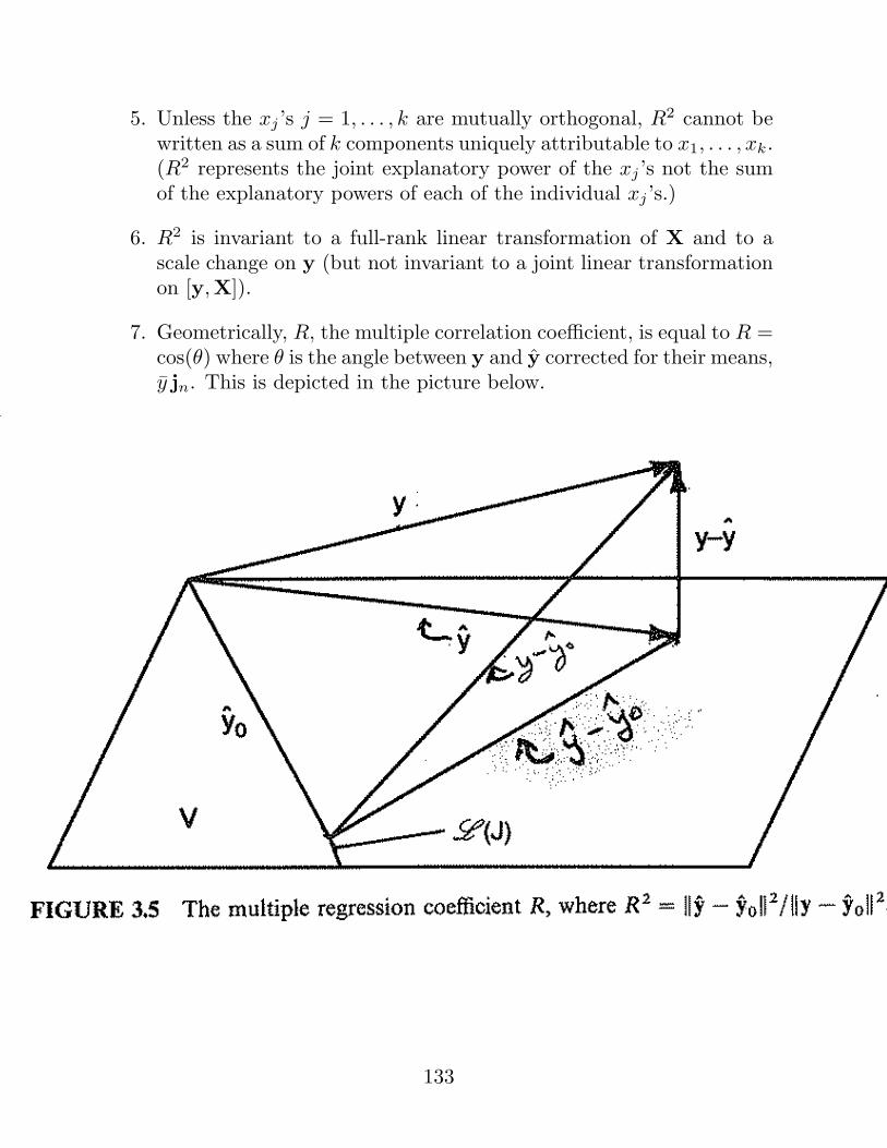
5. Unless the xj ’s j = 1, . . . , k are mutually orthogonal, R2 cannot bewritten as a sum of k components uniquely attributable to x1, . . . , xk.(R2 represents the joint explanatory power of the xj ’s not the sumof the explanatory powers of each of the individual xj ’s.)

6. R2 is invariant to a full-rank linear transformation of X and to ascale change on y (but not invariant to a joint linear transformationon [y,X]).

7. Geometrically, R, the multiple correlation coefficient, is equal to R =cos(θ) where θ is the angle between y and y corrected for their means,y jn. This is depicted in the picture below.

133

Inference in the Multiple Regression Model

Testing a Subset of β: Testing Nested Models

All testing of linear hypotheses (nonlinear hypotheses are rarely encoun-tered in practice) in linear models reduces essentially to putting linearconstraints on the model space. The test amounts to comparing the re-sulting constrained model against the original unconstrained model.

We start with a model we know (assume, really) to be valid:

y = µ + e, where µ = Xβ ∈ C(X) ≡ V, e ∼ Nn(0, σ2In)

and then ask the question of whether or not a simpler model holds corre-sponding to µ ∈ V0 where V0 is a proper subset of V . (E.g., V0 = C(X0)where X0 is a matrix consisting of a subset of the columns of X.)

For example, consider the second order response surface model

yi = β0 +β1xi1 +β2xi2 +β3x2i1 +β4x

2i2 +β5xi1xi2 +ei, i = 1, . . . , n. (†)

This model says that E(y) is a quadratic function of x1 and x2.

A hypothesis we might be interested in here is that the second-order termsare unnecessary; i.e., we might be interested in H0 : β3 = β4 = β5 = 0,under which the model is linear in x1 and x2:

yi = β∗0 + β∗1xi1 + β∗2xi2 + e∗i , i = 1, . . . , n. (‡)

• Testing H0 : β3 = β4 = β5 = 0 is equivalent to testing H0 :model (‡)holds versus H1 :model (†) holds but (‡) does not.

• I.e., we test H0 : µ ∈ C([ jn,x1,x2]) versus

H1 : µ ∈ C([ jn,x1,x2,x1∗x1,x2∗x2,x1∗x2]) and µ /∈ C([ jn,x1,x2]).

Here ∗ denotes the element-wise product and µ = E(y).

134

Without loss of generality, we can always arrange the linear model so theterms we want to test appear last in the linear predictor. So, we write ourmodel as

y = Xβ + e = (X1,X2)(

β1

β2

)+ e

= X1︸︷︷︸n×(k+1−h)

β1 + X2︸︷︷︸n×h

β2 + e, e ∼ N(0, σ2I) (FM)

where we are interested in the hypothesis H0 : β2 = 0.

Under H0 : β2 = 0 the model becomes

y = X1β∗1 + e∗, e∗ ∼ N(0, σ2I) (RM)

The problem is to test

H0 : µ ∈ C(X1) (RM) versus H1 : µ /∈ C(X1)

under the maintained hypothesis that µ ∈ C(X) = C([X1,X2]) (FM).

We’d like to find a test statistic whose size measures the strength of theevidence against H0. If that evidence is overwhelming (the test statisticis large enough) then we reject H0.

The test statistic should be large, but large relative to what?

Large relative to its distribution under the null hypothesis.

How large?

That’s up to the user, but an α−level test rejects H0 if, assuming H0 istrue, the probability of getting a test statistic at least as far from expectedas the one obtained (the p−value) is less than α.

135

• E.g., suppose we compute a test statistic and obtain a p−value ofp = 0.02. This says that assuming H0 is true, the results that weobtained were very unlikely (results this extreme should happen only2% of the time). If these results are so unlikely assuming H0 is true,perhaps H0 is not true. The cut-off for how unlikely our results mustbe before we’re willing to reject H0 is the significance level α. (Wereject if p < α.)

So, we want a test statistic that measures the strength of the evidenceagainst H0 : µ ∈ C(X1) (i.e., one that is small for µ ∈ C(X1) and largefor µ /∈ C(X1)) whose distribution is available.

• This will lead to an F test which is equivalent to the likelihood ratiotest, and which has some optimality properties.

Note that under RM, µ ∈ C(X1) ⊂ C(X) = C([X1,X2]). Therefore, ifRM is true, then FM must be true as well. So, if RM is true, then theleast squares estimates of the mean µ: PC(X1)y and PC(X)y are estimatesof the same thing.

This suggests that the difference between the two estimates

PC(X)y −PC(X1)y = (PC(X) −PC(X1))y

should be small under H0 : µ ∈ C(X1).

• Note that PC(X) −PC(X1) is the projection matrix onto C(X1)⊥ ∩C(X), the orthogonal complement of C(X1) with respect to C(X),and C(X1) ⊕ [C(X1)⊥ ∩ C(X)] = C(X). (See bottom of p. 43 ofthese notes.)

So, under H0, (PC(X) − PC(X1))y should be “small”. A measure of the“smallness” of this vector is its squared length:

‖(PC(X) −PC(X1))y‖2 = yT (PC(X) −PC(X1))y.

136

By our result on expected values of quadratic forms,

E[yT (PC(X) −PC(X1))y] = σ2 dim[C(X1)⊥ ∩ C(X)] + µT (PC(X) −PC(X1))µ

= σ2h + [(PC(X) −PC(X1))µ]T [(PC(X) −PC(X1))µ]

= σ2h + (PC(X)µ−PC(X1)µ)T (PC(X)µ−PC(X1)µ)

Under H0, µ ∈ C(X1) and µ ∈ C(X), so

(PC(X)µ−PC(X1)µ) = µ− µ = 0.

Under H1,PC(X)µ = µ, but PC(X1)µ 6= µ.

I.e., letting µ0 denote p(µ|C(X1)),

E[yT (PC(X) −PC(X1))y] ={

σ2h, under H0;σ2h + ‖µ− µ0‖2, under H1.

• That is, under H0 we expect the squared length of

PC(X)y −PC(X1)y ≡ y − y0

to be small, on the order of σ2h. If H0 is not true, then the squaredlength of y− y0 will be larger, with expected value σ2h+‖µ−µ0‖2.

Therefore, if σ2 is known

‖y − y0‖2σ2h

=‖y − y0‖2/h

σ2

{≈ 1, under H0

> 1, under H1

is an appropriate test statistic for testing H0.

137

Typically, σ2 will not be known, so it must be estimated. The appropriateestimator is s2 = ‖y− y‖2/(n− k− 1), the mean squared error from FM,the model which is valid under H0 and under H1. Our test statistic thenbecomes

F =‖y − y0‖2/h

s2=

‖y − y0‖2/h

‖y − y‖2/(n− k − 1)

{≈ 1, under H0

> 1, under H1.

By the theorems on pp. 84–85, the following results on the numerator anddenominator of F hold:

Theorem: Suppose y ∼ N(Xβ, σ2I) where X is n × (k + 1) of full rankwhere Xβ = X1β1+X2β2, and X2 is n×h. Let y = p(y|C(X)) = PC(X)y,y0 = p(y|C(X1)) = PC(X1)y, and µ0 = p(µ|C(X1)) = PC(X1)µ. Then

(i) 1σ2 ‖y − y‖2 = 1

σ2 yT (I−PC(X))y ∼ χ2(n− k − 1);

(ii) 1σ2 ‖y − y0‖2 = 1

σ2 yT (PC(X) −PC(X1))y ∼ χ2(h, λ1), where

λ1 =1

2σ2‖(PC(X) −PC(X1))µ‖2 =

12σ2

‖µ− µ0‖2;

and

(iii) 1σ2 ‖y − y‖2 and 1

σ2 ‖y − y0‖2 are independent.

Proof: Parts (i) and (ii) folllow immediately from part (3) of the theoremon p. 84. Part (iii) follows because

‖y − y‖2 = ||p(y|C(X)⊥)||2

and‖y − y0‖2 = ||p(y|C(X1)⊥ ∩ C(X)︸ ︷︷ ︸

⊂C(X)

)||2

are squared lengths of projections onto orthogonal subspaces, so they areindependent according to the theorem on p. 85.

138

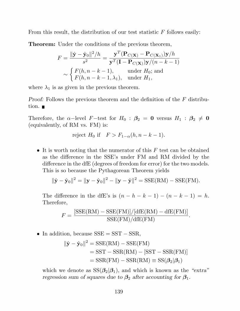
From this result, the distribution of our test statistic F follows easily:

Theorem: Under the conditions of the previous theorem,

F =‖y − y0‖2/h

s2=

yT (PC(X) −PC(X1))y/h

yT (I−PC(X))y/(n− k − 1)

∼{

F (h, n− k − 1), under H0; andF (h, n− k − 1, λ1), under H1,

where λ1 is as given in the previous theorem.

Proof: Follows the previous theorem and the definition of the F distribu-tion.

Therefore, the α−level F−test for H0 : β2 = 0 versus H1 : β2 6= 0(equivalently, of RM vs. FM) is:

reject H0 if F > F1−α(h, n− k − 1).

• It is worth noting that the numerator of this F test can be obtainedas the difference in the SSE’s under FM and RM divided by thedifference in the dfE (degrees of freedom for error) for the two models.This is so because the Pythagorean Theorem yields

‖y − y0‖2 = ‖y − y0‖2 − ‖y − y‖2 = SSE(RM)− SSE(FM).

The difference in the dfE’s is (n − h − k − 1) − (n − k − 1) = h.Therefore,

F =[SSE(RM)− SSE(FM)]/[dfE(RM)− dfE(FM)]

SSE(FM)/dfE(FM).

• In addition, because SSE = SST− SSR,

‖y − y0‖2 = SSE(RM)− SSE(FM)= SST− SSR(RM)− [SST− SSR(FM)]= SSR(FM)− SSR(RM) ≡ SS(β2|β1)

which we denote as SS(β2|β1), and which is known as the “extra”regression sum of squares due to β2 after accounting for β1.

139

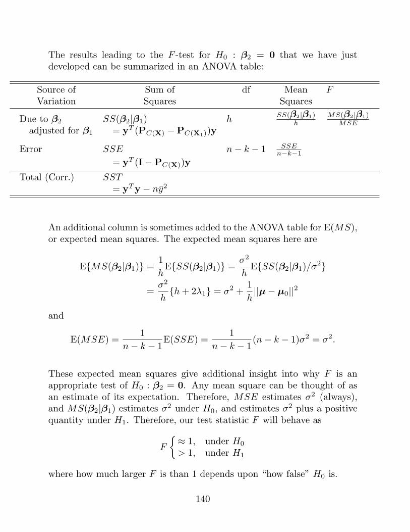
The results leading to the F -test for H0 : β2 = 0 that we have justdeveloped can be summarized in an ANOVA table:

Source of Sum of df Mean FVariation Squares Squares

Due to β2 SS(β2|β1) hSS(β2|β1)

hMS(β2|β1)

MSEadjusted for β1 = yT (PC(X) −PC(X1))y

Error SSE n− k − 1 SSEn−k−1

= yT (I−PC(X))y

Total (Corr.) SST= yT y − ny2

An additional column is sometimes added to the ANOVA table for E(MS),or expected mean squares. The expected mean squares here are

E{MS(β2|β1)} =1h

E{SS(β2|β1)} =σ2

hE{SS(β2|β1)/σ2}

=σ2

h{h + 2λ1} = σ2 +

1h||µ− µ0||2

and

E(MSE) =1

n− k − 1E(SSE) =

1n− k − 1

(n− k − 1)σ2 = σ2.

These expected mean squares give additional insight into why F is anappropriate test of H0 : β2 = 0. Any mean square can be thought of asan estimate of its expectation. Therefore, MSE estimates σ2 (always),and MS(β2|β1) estimates σ2 under H0, and estimates σ2 plus a positivequantity under H1. Therefore, our test statistic F will behave as

F

{≈ 1, under H0

> 1, under H1

where how much larger F is than 1 depends upon “how false” H0 is.

140

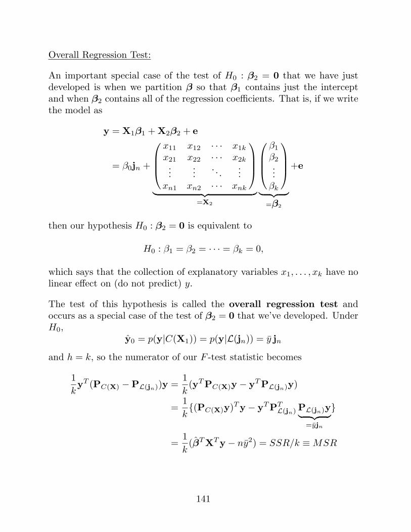
Overall Regression Test:

An important special case of the test of H0 : β2 = 0 that we have justdeveloped is when we partition β so that β1 contains just the interceptand when β2 contains all of the regression coefficients. That is, if we writethe model as

y = X1β1 + X2β2 + e

= β0jn +

x11 x12 · · · x1k

x21 x22 · · · x2k...

.... . .

...xn1 xn2 · · · xnk

︸ ︷︷ ︸=X2

β1

β2...

βk

︸ ︷︷ ︸=β2

+e

then our hypothesis H0 : β2 = 0 is equivalent to

H0 : β1 = β2 = · · · = βk = 0,

which says that the collection of explanatory variables x1, . . . , xk have nolinear effect on (do not predict) y.

The test of this hypothesis is called the overall regression test andoccurs as a special case of the test of β2 = 0 that we’ve developed. UnderH0,

y0 = p(y|C(X1)) = p(y|L(jn)) = y jn

and h = k, so the numerator of our F -test statistic becomes

1kyT (PC(X) −PL(jn))y =

1k

(yT PC(X)y − yT PL(jn)y)

=1k{(PC(X)y)T y − yT PT

L(jn) PL(jn)y︸ ︷︷ ︸=yjn

}

=1k

(βT XT y − ny2) = SSR/k ≡ MSR

141

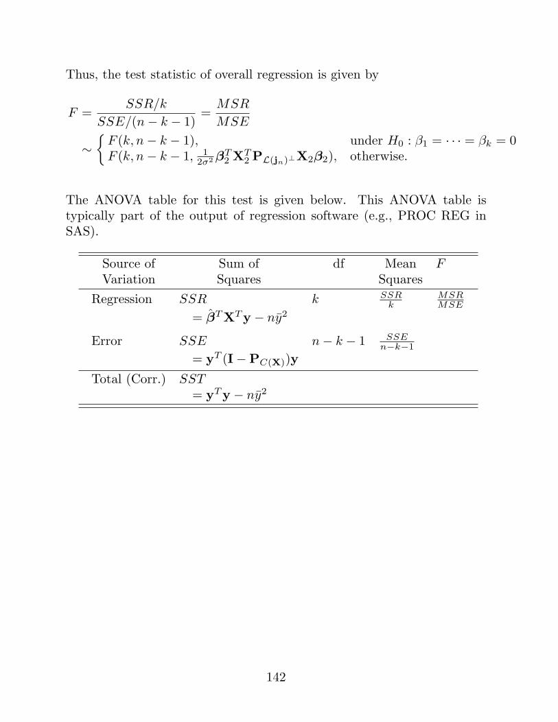
Thus, the test statistic of overall regression is given by

F =SSR/k

SSE/(n− k − 1)=

MSR

MSE

∼{

F (k, n− k − 1), under H0 : β1 = · · · = βk = 0F (k, n− k − 1, 1

2σ2 βT2 XT

2 PL(jn)⊥X2β2), otherwise.

The ANOVA table for this test is given below. This ANOVA table istypically part of the output of regression software (e.g., PROC REG inSAS).

Source of Sum of df Mean FVariation Squares Squares

Regression SSR k SSRk

MSRMSE

= βT XT y − ny2

Error SSE n− k − 1 SSEn−k−1

= yT (I−PC(X))y

Total (Corr.) SST= yT y − ny2

142

F test in terms of R2:

The F test statistics we have just developed can be written in terms of R2,the coefficient of determination. This relationship is given by the followingtheorem.

Theorem: The F statistic for testing H0 : β2 = 0 in the full rank modely = X1β1 + X2β2 + e (top of p. 138) can be written in terms of R2 as

F =(R2

FM −R2RM )/h

(1−R2FM )/(n− k − 1)

,

where R2FM corresponds to the full model y = X1β1+X2β2+e, and R2

RM

corresponds to the reduced model y = X1β∗1 + e∗.

Proof: Homework.

Corollary: The F statistic for overall regression (for testing H0 : β1 =β2 = · · · = βk = 0) in the full rank model, yi = β0+β1xi1+· · ·+βkxik +ei,

i = 1, . . . , n, e1, . . . , eniid∼ N(0, σ2) can be written in terms of R2, the

coefficient of determination from this model as follows:

F =R2/k

(1−R2)/(n− k − 1).

Proof: For this hypothesis h, the dimension of the regression parameterbeing tested, is k. In addition, the reduced model here is

y = jnβ0 + e,

so (Xβ)RM , the estimated mean of y, under the reduced model is (Xβ)RM =jny. So, R2

RM in the previous theorem is (cf. p. 131):

R2RM =

[(Xβ)TRMy − ny2]

yT y − ny2

=[y

=ny︷︸︸︷jTny −ny2]

yT y − ny2= 0.

The result now follows from the previous theorem.

143

The General Linear Hypothesis H0 : Cβ = t

The hypothesis H0 : Cβ = t is called the general linear hypothesis. HereC is a q × (k + 1) matrix of (known) coefficients with rank(C) = q. Wewill consider the slightly simpler case H : Cβ = 0 (i.e., t = 0) first.

Most of the questions that are typically asked about the coefficients of alinear model can be formulated as hypotheses that can be written in theform H0 : Cβ = 0, for some C. For example, the hypothesis H0 : β2 = 0in the model

y = X1β1 + X2β2 + e, e ∼ N(0, σ2I)

can be written as

H0 : Cβ = ( 0︸︷︷︸h×(k+1−h)

, Ih)(

β1

β2

)= β2 = 0.

The test of overall regression can be written as

H0 : Cβ = ( 0︸︷︷︸k×1

, Ik)

β0

β1...

βk

=

β1...

βk

= 0.

Hypotheses encompassed by H:Cβ = 0 are not limitted to ones in whichcertain regression coefficients are set equal to zero. Another example thatcan be handled is the hypothesis H0 : β1 = β2 = · · · = βk. For example,suppose k = 4, then this hypothesis can be written as

H0 : Cβ =

0 1 −1 0 00 0 1 −1 00 0 0 1 −1

β0

β1

β2

β3

β4

=

β1 − β2

β2 − β3

β3 − β4

= 0.

Another equally good choice for C in this example is

C =

0 1 −1 0 00 1 0 −1 00 1 0 0 −1

144

The test statistic for H0 : Cβ = 0 is based on comparing Cβ to its nullvalue 0, using a squared statistical distance (quadratic form) of the form

Q = {Cβ − E0(Cβ)︸ ︷︷ ︸=0

}T {var0(Cβ)}−1{Cβ − E0(Cβ)}

= (Cβ)T {var0(Cβ)}−1(Cβ).

• Here, the 0 subscript is there to indicate that the expected value andvariance are computed under H0.

Recall that β ∼ Nk+1(β, σ2(XT X)−1). Therefore,

Cβ ∼ Nq(Cβ, σ2C(XT X)−1CT ).

We estimate σ2 using s2 = MSE = SSE/(n− k − 1), so

var0(Cβ) = s2C(XT X)−1CT

and Q becomes

Q = (Cβ)T {s2C(XT X)−1CT }−1Cβ

=(Cβ)T {C(XT X)−1CT }−1Cβ

SSE/(n− k − 1)

145

To use Q to form a test statistic, we need its distribution, which is givenby the following theorem:

Theorem: If y ∼ Nn(Xβ, σ2In) where X is n × (k + 1) of full rank andC is q × (k + 1) of rank q ≤ k + 1, then

(i) Cβ ∼ Nq[Cβ, σ2C(XT X)−1CT ];(ii) (Cβ)T [C(XT X)−1CT ]−1Cβ/σ2 ∼ χ2(q, λ), where

λ = (Cβ)T [C(XT X)−1CT ]−1Cβ/(2σ2);

(iii) SSE/σ2 ∼ χ2(n− k − 1); and(iv) (Cβ)T [C(XT X)−1CT ]−1Cβ and SSE are independent.

Proof: Part (i) follows from the normality of β and that Cβ is an affinetransformation of a normal. Part (iii) has been proved previously (p. 138).

(ii) Recall the theorem on the bottom of p. 82 (thm 5.5A in our text).This theorem said that if y ∼ Nn(µ,Σ) and A was n× n of rank r,then yT Ay ∼ χ2(r, 1

2µT Aµ) iff AΣ is idempotent. Here Cβ playsthe role of y, Cβ plays the role of µ, σ2C(XT X)−1CT plays the roleof Σ, and {σ2C(XT X)−1CT }−1 plays the role of A. Then the resultfollows because AΣ = {σ2C(XT X)−1CT }−1σ2C(XT X)−1CT = Iis obviously idempotent.

(iv) Since β and SSE are independent (p. 115) then (Cβ)T [C(XT X)−1CT ]−1Cβ

(a function of β) and SSE must be independent.

Therefore,

F = Q/q =(Cβ)T {C(XT X)−1CT }−1Cβ/q

SSE/(n− k − 1)=

SSH/q

SSE/(n− k − 1)

has the form of a ratio of independent χ2’s each divided by its d.f.

• Here, SSH denotes (Cβ)T {C(XT X)−1CT }−1Cβ, the sum of squaresdue to the Hypothesis H0.

146

Theorem: If y ∼ Nn(Xβ, σ2In) where X is n × (k + 1) of full rank andC is q × (k + 1) of rank q ≤ k + 1, then

F =(Cβ)T {C(XT X)−1CT }−1Cβ/q

SSE/(n− k − 1)

=SSH/q

SSE/(n− k − 1)

∼{

F (q, n− k − 1), if H0 : Cβ = 0 is true;F (q, n− k − 1, λ), if H0 : Cβ = 0 is false,

where λ is as in the previous theorem.

Proof: Follows from the previous theorem and the definition of the Fdistribution.

So, to conduct a hypothesis test of H0 : Cβ = 0, we compute F and rejectat level α if F > F1−α(q, n− k − 1) (F1−α denotes the (1− α)th quantile,or upper αth quantile of the F distribution).

147

The general linear hypothesis as a test of nested models:

We have seen that the test of β2 = 0 in the model y = X1β1 + X2β2 + ecan be formulated as a test of Cβ = 0. Therefore, special cases of thegeneral linear hypothesis correspond to tests of nested (full and reduced)models. In fact, all F tests of the general linear hypothesis H0 : Cβ = 0can be formulated as tests of nested models.

Theorem: The F test for the general linear hypothesis H0 : Cβ = 0 is afull-and-reduced-model test.

Proof: The book, in combination with a homework problem, provides aproof based on Lagrange multipliers. Here we offer a different proof basedon geometry.

Under H0,

y = Xβ + e and Cβ = 0

⇒ C(XT X)−1XT Xβ = 0

⇒ C(XT X)−1XT µ = 0

⇒ TT µ = 0 where T = X(XT X)−1CT .

That is, under H0, µ = Xβ ∈ C(X) = V and µ ⊥ C(T), or

µ ∈ [C(T)⊥ ∩ C(X)] = V0

where V0 = C(T)⊥ ∩ C(X) is the orthogonal complement of C(T) withrespect to C(X).

• Thus, under H0 : Cβ = 0, µ ∈ V0 ⊂ V = C(X), and under H1 :Cβ 6= 0, µ ∈ V but µ /∈ V0. That is, these hypotheses correspondto nested models. It just remains to establish that the F test forthese nested models is the F test for the general linear hypothesisH0 : Cβ = 0 given on p. 147.

148

The F test statistic for nested models given on p. 139 is

F =yT (PC(X) −PC(X1))y/h

SSE/(n− k − 1)

Here, we replace PC(X1) by the projection matrix onto V0:

PV0 = PC(X) −PC(T)

and replace h with dim(V ) − dim(V0), the reduction in dimension of themodel space when we go from the full to the reduced model.

Since V0 is the orthogonal complement of C(T) with respect to C(X),dim(V0) is given by

dim(V0) = dim(C(X))− dim(C(T)) = rank(X)− rank(T) = k + 1− q

Here, rank(T) = q by the following argument:

rank(T) = rank(TT ) ≥ rank(TT X) = rank(C(XT X)−1XT X) = rank(C) = q

and

rank(T) = rank(TT T) = rank(C(XT X)−1XT X(XT X)−1CT )

= rank(C(XT X)−1CT

︸ ︷︷ ︸q×q

) ≤ q.

Therefore, q ≤ rank(T) ≤ q ⇒ rank(T) = q.

So,h = dim(V )− dim(V0) = (k + 1)− [(k + 1)− q] = q.

149

Thus the full vs. reduced model F statistic becomes

F =yT [PC(X) −PV0 ]y/q

SSE/(n− k − 1)=

yT [PC(X) − (PC(X) −PC(T))]y/q

SSE/(n− k − 1)

=yT PC(T)y/q

SSE/(n− k − 1)

where

yT PC(T)y = yT T(TT T)−1TT y

= yT X(XT X)−1CT {C(XT X)−1XT X(XT X)−1CT }−1C(XT X)−1XT y

= yT X(XT X)−1

︸ ︷︷ ︸=

ˆβT

CT {C(XT X)−1CT }−1C (XT X)−1XT y︸ ︷︷ ︸=

ˆβ

= βT CT {C(XT X)−1CT }−1Cβ

which is our test statistic for the general linear hypothesis H0 : Cβ = 0from p. 147.

The case H0 : Cβ = t where t 6= 0:

Extension to this case is straightforward. The only requirement is that thesystem of equations Cβ = t be consistent, which is ensured by C havingfull row rank q.

Then the F test statistic for H0 : Cβ = t is given by

F =(Cβ − t)T [C(XT X)−1CT ]−1(Cβ − t)/q

SSE/(n− k − 1)∼

{F (q, n− k − 1), under H0

F (q, n− k − 1, λ), otherwise,

where λ = (Cβ − t)T [C(XT X)−1CT ]−1(Cβ − t)/(2σ2).

150

Tests on βj and on aT β:

Tests of H0 : βj = 0 or H0 : aT β = 0 occur as special cases of the testswe have already considered. To test H0 : aT β = 0, we use aT in place ofC in our test of the general linear hypothesis Cβ = 0. In this case q = 1and the test statistic becomes

F =(aT β)T [aT (XT X)−1a]−1aT β

SSE/(n− k − 1)=

(aT β)2

s2aT (XT X)−1a

∼ F (1, n− k − 1) under H0 : aT β = 0.

• Note that since t2(ν) = F (1, ν), an equivalent test of H0 : aT β = 0is given by the t-test with test statistic

t =aT β

s√

aT (XT X)−1a∼ t(n− k − 1) under H0.

An important special case of the hypothesis H0 : aT β = 0 occurs whena = (0, . . . , 0, 1, 0, . . . , 0)T where the 1 appears in the j+1th position. Thisis the hypothesis H0 : βj = 0, and it says that the jth explanatory variablexj has no partial regression effect on y (no effect above and beyond theeffects of the other explanatory variables in the model).

The test statistic for this hypothesis simplifies from that given above toyield

F =β2

j

s2gjj∼ F (1, n− k − 1) under H0 : βj = 0,

where gjj is the jth diagonal element of (XT X)−1. Equivalently, we coulduse the t test statistic

t =βj

s√

gjj=

βj

s.e.(βj)∼ t(n− k − 1) under H0 : βj = 0.

151

Confidence and Prediction Intervals

Hypothesis tests and confidence regions (e.g., intervals) are really two dif-ferent ways to look at the same problem.

• For an α-level test of a hypothesis of the form H0 : θ = θ0, a100(1 − α)% confidence region for θ is given by all those values ofθ0 such that the hypothesis would not be rejected. That is, theacceptance region of the α-level test is the 100(1 − α)% confidenceregion for θ.

• Conversely, θ0 falls outside of a 100(1−α)% confidence region for θiff an α level test of H0 : θ = θ0 is rejected.

• That is, we can invert the statistical tests that we have derived toobtain confidence regions for parameters of the linear model.

Confidence Region for β:

If we set C = Ik+1 and t = β in the F statistic on the bottom of p. 150,we obtain

(β − β)T XT X(β − β)/(k + 1)s2

∼ F (k + 1, n− k − 1)

From this distributional result, we can make the probability statement,

Pr

{(β − β)T XT X(β − β)

s2(k + 1)≤ F1−α(k + 1, n− k − 1)

}= 1− α.

Therefore, the set of all vectors β that satisfy

(β − β)T XT X(β − β) ≤ (k + 1)s2F1−α(k + 1, n− k − 1)

forms a 100(1− α)% confidence region for β.

152

• Such a region is an ellipse, and is only easy to draw and make easyinterpretation of for k = 1 (e.g., simple linear regression).

• If one can’t plot the region and then plot a point to see whether itsin or out of the region (i.e., for k > 1) then this region isn’t any moreinformative than the test of H0 : β = β0. To decide whether β0 isin the region, we essentially have to perform the test!

• More useful are confidence intervals for the individual βj ’s and forlinear combinations of the form aT β.

Confidence Interval for aT β:

If we set C = aT and t = aT β in the F statistic on the bottom of p. 150,we obtain

(aT β − aT β)2

s2aT (XT X)−1a∼ F (1, n− k − 1)

which implies(aT β − aT β)

s√

aT (XT X)−1a∼ t(n− k − 1).

From this distributional result, we can make the probability statement,

Pr

tα/2(n− k − 1)︸ ︷︷ ︸−t1−α/2(n−k−1)

≤ (aT β − aT β)s√

aT (XT X)−1a≤ t1−α/2(n− k − 1)

= 1− α.

Rearranging this inequality so that aT β falls in the middle, we get

Pr{aT β − t1−α/2(n− k − 1)s

√aT (XT X)−1a ≤ aT β

≤ aT β + t1−α/2(n− k − 1)s√

aT (XT X)−1a}

= 1− α.

Therefore, a 100(1− α)% CI for aT β is given by

aT β ± t1−α/2(n− k − 1)s√

aT (XT X)−1a.

153

Confidence Interval for βj:

A special case of this interval occurs when a = (0, . . . , 0, 1, 0, . . . , 0)T ,where the 1 is in the j + 1th position. In this case aT β = βj , aT β = βj ,and aT (XT X)−1a = {(XT X)−1}jj ≡ gjj . The confidence interval for βj

is then given byβj ± t1−α/2(n− k − 1)s

√gjj .

Confidence Interval for E(y):

Let x0 = (1, x01, x02, . . . , x0k)T denote a particular choice of the vectorof explanatory variables x = (1, x1, x2, . . . , xk)T and let y0 denote thecorresponding response.

We assume that the model y = Xβ + e, e ∼ N(0, σ2I) applies to (y0,x0)as well. This may be because (y0,x0) were in the original sample to whichthe model was fit (i.e., xT

0 is a row of X), or because we believe that(y0,x0) will behave similarly to the data (y,X) in the sample. Then

y0 = xT0 β + e0, e0 ∼ N(0, σ2)

where β and σ2 are the same parameters in the fitted model y = Xβ + e.

Suppose we wish to find a CI for

E(y0) = xT0 β.

This quantity is of the form aT β where a = x0, so the BLUE of E(y0) isxT

0 β and a 100(1− α)% CI for E(y0) is given by

xT0 β ± t1−α/2(n− k − 1)s

√xT

0 (XT X)−1x0.

154

• This confidence interval holds for a particular value xT0 β. Sometimes,

it is of interest to form simultaneous confidence intervals around eachand every point xT

0 β for all x0 in the range of x. That is, we some-times desire a simultaneous confidence band for the entire regressionline (or plane, for k > 1). The confidence interval given above, ifplotted for each value of x0, does not give such a simultaneous band;instead it gives a “point-wise” band. For discussion of simultaneousintervals see §8.6.7 of our text.

• The confidence interval given above is for E(y0), not for y0 itself.E(y0) is a parameter, y0 is a random variable. Therefore, we can’testimate y0 or form a confidence interval for it. However, we can pre-dict its value, and an interval around that prediction that quantifiesthe uncertainty associated with that prediction is called a predictioninterval.

Prediction Interval for an Unobserved y-value:

For an unobserved value y0 with known explanatory vector x0 assumed tofollow our linear model y = Xβ + e, we predict y0 by

y0 = xT0 β.

• Note that this predictor of y0 coincides with our estimator of E(y0).However, the uncertainty associated with the quantity xT

0 β as apredictor of y0 is different from (greater than) its uncertainty as anestimator of E(y0). Why? Because observations (e.g., y0) are morevariable than their means (e.g., E(y0)).

155

To form a CI for the estimator xT0 β of E(y0) we examine the variance of

the error of estimation:

var{E(y0)− xT0 β} = var(xT

0 β).

In contrast, to form a PI for the predictor xT0 β of y0, we examine the

variance of the error of prediction:

var(y0 − xT0 β) = var(y0) + var(xT

0 β)− 2 cov(y0,xT0 β)︸ ︷︷ ︸

0

= var(xT0 β + e0) + var(xT

0 β)

= var(e0) + var(xT0 β) = σ2 + σ2xT

0 (XT X)−1x0.

Since σ2 is unknown, we must estimate this quantity with s2, yielding

var(y0 − y0) = s2{1 + xT0 (XT X)−1x0}.

It’s not hard to show thaty0 − y0

s√

1 + xT0 (XT X)−1x0

∼ t(n− k − 1),

therefore

Pr

{−t1−α/2(n− k − 1) ≤ y0 − y0

s√

1 + xT0 (XT X)−1x0

≤ t1−α/2(n− k − 1)

}= 1−α.

Rearranging,

Pr{

y0 − t1−α/2(n− k − 1)s√

1 + xT0 (XT X)−1x0 ≤ y0

≤ y0 + t1−α/2(n− k − 1)s√

1 + xT0 (XT X)−1x0

}= 1− α.

Therefore, a 100(1− α)% prediction interval for y0 is given by

y0 ± t1−α/2(n− k − 1)s√

1 + xT0 (XT X)−1x0.

• Once again, this is a point-wise interval. Simultaneous predictionintervals for predicting multiple y-values with given coverage proba-bility are discussed in §8.6.7.

156

Equivalence of the F−test and Likelihood Ratio Test:

Recall that for the classical linear model y = Xβ + e, with normal, ho-moscedastic errors, the likelihood function is given by

L(β, σ2;y) = (2πσ2)−n/2 exp{−‖y −Xβ‖2/(2σ2)},

or expressing the likelihood as a function of µ = Xβ instead of β:

L(µ, σ2;y) = (2πσ2)−n/2 exp{−‖y − µ‖2/(2σ2)}.

• L(µ, σ2;y) gives the probability of observing y for specified valuesof the parameters µ and σ2 (to be more precise, the probability thatthe response vector is “close to” the observed value y).

– or, roughly, it measures how likely the data are for given valuesof the parameters.

The idea behind a likelihood ratio test (LRT) for some hypothesis H0 is tocompare the likelihood function maximized over the parameters subject tothe restriction imposed by H0 (the constrained maximum likelihood) withthe likelihood function maximized over the parameters without assumingH0 is true (the unconstrained maximum likelihood).

• That is, we compare how probable the data are under the most favor-able values of the parameters subject to H0 (the constrained MLEs),with how probable the data are under the most favorable values ofthe parameters under the maintained hypothesis (the unconstrainedMLEs).

• If assuming H0 makes the data substantially less probable than notassuming H0, then we reject H0.

157

Consider testing H0 : µ ∈ V0 versus H1 : µ /∈ V0 under the maintainedhypothesis that µ is in V . Here V0 ⊂ V and dim(V0) = k+1−h ≤ k+1 =dim(V ).

Let y = p(y|V ) and y0 = p(y|V0). Then the unconstrained MLEs of(µ, σ2) are µ = y and σ2 = ‖y − y‖2/n and the constrained MLEs areµ0 = y0 and σ2

0 = ‖y − y0‖2/n.

Therefore, the likelihood ratio statistic is

LR =supµ∈V0

L(µ,σ2;y)supµ∈V L(µ, σ2;y)

=L(y0, σ

20)

L(y, σ2)

=(2πσ2

0)−n/2 exp{−‖y − y0‖2/(2σ20)}

(2πσ2)−n/2 exp{−‖y − y‖2/(2σ2)}

=(

σ20

σ2

)−n/2 exp(−n/2)exp(−n/2)

=(

σ20

σ2

)−n/2

• We reject for small values of LR. Typically in LRTs, we work withλ = −2 log(LR) so that we can reject for large values of λ. In thiscase, λ = n log

(σ2

0/σ2).

• Equivalently we reject for large values of(σ2

0/σ2)

where

(σ2

0

σ2

)=‖y − y0‖2‖y − y‖2 =

‖y − y‖2 + ‖y − y0‖2‖y − y‖2

= 1 +‖y − y0‖2‖y − y‖2 = 1 +

(h

n− k − 1

)F

a monotone function of F (cf. the F statistic on the top of p. 138).

Therefore, large values of λ correspond to large values of F and the decisionrules based on LR and on F are the same.

• Therefore, the LRT and the F−test are equivalent.

158

Analysis of Variance Models: The Non-Full Rank Linear Model

• To this point, we have focused exclusively on the case when themodel matrix X of the linear model is of full rank. We now considerthe case when X is n× p with rank(X) = k < p.

• The basic ideas behind estimation and inference in this case are thesame as in the full rank case, but the fact that (XT X)−1 doesn’texist and therefore the normal equations have no unique solutioncauses a number of technical complications.

• We wouldn’t bother to dwell on these technicalities if it weren’t forthe fact that the non-full rank case does arise frequently in applica-tions in the form of analysis of variance models .

The One-way Model:

Consider the balanced one-way layout model for yij a response on the jth

unit in the ith treatment group. Suppose that there are a treatments and nunits in the ith treatment group. The cell-means model for this situationis

yij = µi + eij , i = 1, . . . , a, j = 1, . . . , n,

where the eij ’s are i.i.d. N(0, σ2).

An alternative, but equivalent, linear model is the effects model for theone-way layout:

yij = µ + αi + eij , i = 1, . . . , a, j = 1, . . . , n,

with the same assumptions on the errors.

159

The cell means model can be written in vector notation as

y = µ1x1 + µ2x2 + · · ·+ µaxa + e, e ∼ N(0, σ2I),

and the effects model can be written as

y = µjN + α1x1 + α2x2 + · · ·+ αaxa + e, e ∼ N(0, σ2I),

where xi is an indicator for treatment i, and N = an is the total samplesize.

• That is, the effects model has the same model matrix as the cell-means model, but with one extra column, a column of ones, in thefirst position.

• Notice that∑

i xi = jN . Therefore, the columns of the model matrixfor the effects model are linearly dependent.

Let X1 denote the model matrix in the cell-means model, X2 = (jN ,X1)denote the model matrix in the effects model.

• Note that C(X1) = C(X2).

In general, two linear models y = X1β1+e1, y = X2β2+e2 with the sameassumptions on e1 and e2 are equivalent linear models if C(X1) = C(X2).

Why?

Because the mean vectors µ1 = X1β1 and µ2 = X2β2 in the two casesare both restricted to fall in the same subspace C(X1) = C(X2).

In addition,µ1 = p(y|C(X1)) = p(y|C(X2)) = µ2

is the same in both models, and

S2 =1

n− dim(C(X1))‖y − µ1‖2 =

1n− dim(C(X2))

‖y − µ2‖2

is the same in both models.

160

• The cell-means and effects models are simply reparameterizations ofone-another. The relationship between the parameters in this caseis very simple: µi = µ + αi, i = 1, . . . , a.

• Let V = C(X1) = C(X2). In the case of the cell-means model,rank(X1) = a = dim(V ) and β1 is a × 1. In the case of the effectsmodel, rank(X2) = a = dim(V ) but β2 is (a + 1) × 1. The effectsmodel is overparameterized.

To understand overparameterization, consider the model

yij = µ + αi + eij , i = 1, . . . , a, j = 1, . . . , n.

This model says that E(yij) = µ + αi = µi, or

E(y1j) = µ + α1 = µ1 j = 1, . . . , n,

E(y2j) = µ + α2 = µ2 j = 1, . . . , n,

...

Suppose the true treatment means are µ1 = 10 and µ2 = 8. In terms ofthe parameters of the effects model, µ and the αi’s, these means can berepresented in an infinity of possible ways,

E(y1j) = 10 + 0 j = 1, . . . , n,

E(y2j) = 10 + (−2) j = 1, . . . , n,

(µ = 10, α1 = 0, and α2 = −2), or

E(y1j) = 8 + 2 j = 1, . . . , n,

E(y2j) = 8 + 0 j = 1, . . . , n,

(µ = 8, α1 = 2, and α2 = 0), or

E(y1j) = 1 + 9 j = 1, . . . , n,

E(y2j) = 1 + 7 j = 1, . . . , n,

(µ = 1, α1 = 9, and α2 = 7), etc.

161

Why would we want to consider an overparameterized model like theeffects model?

In a simple case like the one-way layout, I would argue that we wouldn’t.

The most important criterion for choice of parameterization of a model isinterpretability. Without imposing any constraints, the parameters of theeffects model do not have clear interpretations.

However, subject to the constraint∑

i αi = 0, the parameters of theeffects model have the following interpretations:

µ =grand mean response across all treatmentsαi =deviation from the grand mean placing µi (the ith treatmentmean) up or down from the grand mean; i.e., the effect of the ith

treatment.

Without the constraint, though, µ is not constrained to fall in the centerof the µi’s. µ is in no sense the grand mean, it is just an arbitrary baselinevalue.

In addition, adding the constraint∑

i αi = 0 has essentially the effect ofreparameterizing from the overparameterized (non-full rank) effects modelto a just-parameterized (full rank) model that is equivalent (in the senseof having the same model space) as the cell means model.

To see this consider the one-way effects model with a = 3, n = 2. Then∑ai=1 αi = 0 implies α1 + α2 + α3 = 0 or α3 = −(α1 + α2). Subject to the

constraint, the effects model is

y = µjN + α1x1 + α2x2 + α3x3 + e, where α3 = −(α1 + α2),

162

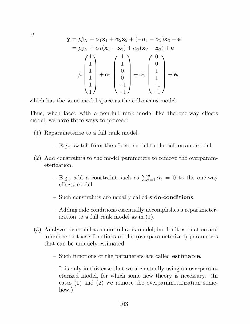
ory = µjN + α1x1 + α2x2 + (−α1 − α2)x3 + e

= µjN + α1(x1 − x3) + α2(x2 − x3) + e

= µ

111111

+ α1

1100−1−1

+ α2

0011−1−1

+ e,

which has the same model space as the cell-means model.

Thus, when faced with a non-full rank model like the one-way effectsmodel, we have three ways to proceed:

(1) Reparameterize to a full rank model.

– E.g., switch from the effects model to the cell-means model.

(2) Add constraints to the model parameters to remove the overparam-eterization.

– E.g., add a constraint such as∑a

i=1 αi = 0 to the one-wayeffects model.

– Such constraints are usually called side-conditions.

– Adding side conditions essentially accomplishes a reparameter-ization to a full rank model as in (1).

(3) Analyze the model as a non-full rank model, but limit estimation andinference to those functions of the (overparameterized) parametersthat can be uniquely estimated.

– Such functions of the parameters are called estimable.

– It is only in this case that we are actually using an overparam-eterized model, for which some new theory is necessary. (Incases (1) and (2) we remove the overparameterization some-how.)

163

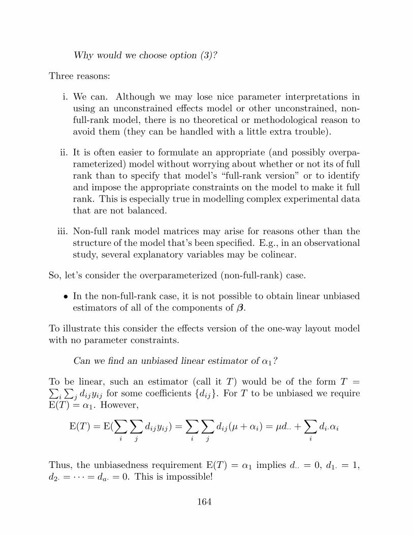
Why would we choose option (3)?

Three reasons:

i. We can. Although we may lose nice parameter interpretations inusing an unconstrained effects model or other unconstrained, non-full-rank model, there is no theoretical or methodological reason toavoid them (they can be handled with a little extra trouble).

ii. It is often easier to formulate an appropriate (and possibly overpa-rameterized) model without worrying about whether or not its of fullrank than to specify that model’s “full-rank version” or to identifyand impose the appropriate constraints on the model to make it fullrank. This is especially true in modelling complex experimental datathat are not balanced.

iii. Non-full rank model matrices may arise for reasons other than thestructure of the model that’s been specified. E.g., in an observationalstudy, several explanatory variables may be colinear.

So, let’s consider the overparameterized (non-full-rank) case.

• In the non-full-rank case, it is not possible to obtain linear unbiasedestimators of all of the components of β.

To illustrate this consider the effects version of the one-way layout modelwith no parameter constraints.

Can we find an unbiased linear estimator of α1?

To be linear, such an estimator (call it T ) would be of the form T =∑i

∑j dijyij for some coefficients {dij}. For T to be unbiased we require

E(T ) = α1. However,

E(T ) = E(∑

i

∑

j

dijyij) =∑

i

∑

j

dij(µ + αi) = µd·· +∑

i

di·αi

Thus, the unbiasedness requirement E(T ) = α1 implies d·· = 0, d1· = 1,d2· = · · · = da· = 0. This is impossible!

164

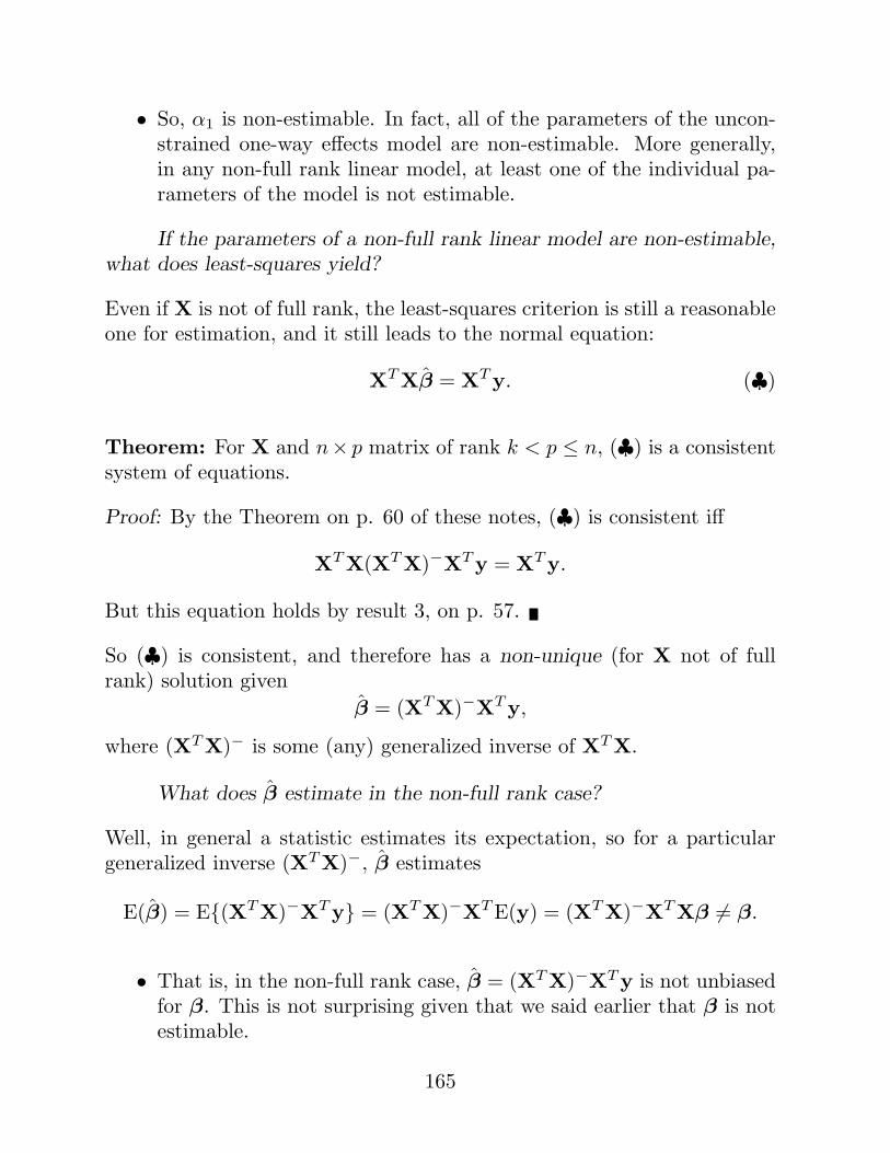
• So, α1 is non-estimable. In fact, all of the parameters of the uncon-strained one-way effects model are non-estimable. More generally,in any non-full rank linear model, at least one of the individual pa-rameters of the model is not estimable.

If the parameters of a non-full rank linear model are non-estimable,what does least-squares yield?

Even if X is not of full rank, the least-squares criterion is still a reasonableone for estimation, and it still leads to the normal equation:

XT Xβ = XT y. (♣)

Theorem: For X and n× p matrix of rank k < p ≤ n, (♣) is a consistentsystem of equations.

Proof: By the Theorem on p. 60 of these notes, (♣) is consistent iff

XT X(XT X)−XT y = XT y.

But this equation holds by result 3, on p. 57.

So (♣) is consistent, and therefore has a non-unique (for X not of fullrank) solution given

β = (XT X)−XT y,

where (XT X)− is some (any) generalized inverse of XT X.

What does β estimate in the non-full rank case?

Well, in general a statistic estimates its expectation, so for a particulargeneralized inverse (XT X)−, β estimates

E(β) = E{(XT X)−XT y} = (XT X)−XT E(y) = (XT X)−XT Xβ 6= β.

• That is, in the non-full rank case, β = (XT X)−XT y is not unbiasedfor β. This is not surprising given that we said earlier that β is notestimable.

165

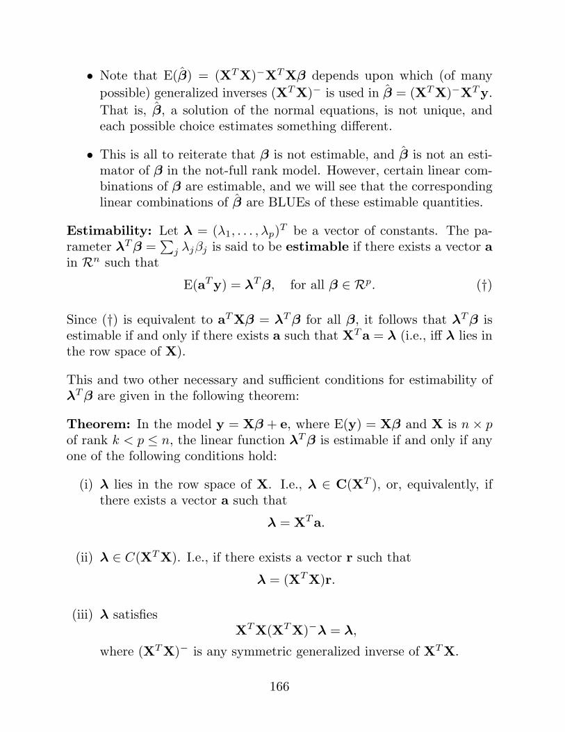
• Note that E(β) = (XT X)−XT Xβ depends upon which (of manypossible) generalized inverses (XT X)− is used in β = (XT X)−XT y.That is, β, a solution of the normal equations, is not unique, andeach possible choice estimates something different.

• This is all to reiterate that β is not estimable, and β is not an esti-mator of β in the not-full rank model. However, certain linear com-binations of β are estimable, and we will see that the correspondinglinear combinations of β are BLUEs of these estimable quantities.

Estimability: Let λ = (λ1, . . . , λp)T be a vector of constants. The pa-rameter λT β =

∑j λjβj is said to be estimable if there exists a vector a

in Rn such that

E(aT y) = λT β, for all β ∈ Rp. (†)

Since (†) is equivalent to aT Xβ = λT β for all β, it follows that λT β isestimable if and only if there exists a such that XT a = λ (i.e., iff λ lies inthe row space of X).

This and two other necessary and sufficient conditions for estimability ofλT β are given in the following theorem:

Theorem: In the model y = Xβ + e, where E(y) = Xβ and X is n × pof rank k < p ≤ n, the linear function λT β is estimable if and only if anyone of the following conditions hold:

(i) λ lies in the row space of X. I.e., λ ∈ C(XT ), or, equivalently, ifthere exists a vector a such that

λ = XT a.

(ii) λ ∈ C(XT X). I.e., if there exists a vector r such that

λ = (XT X)r.

(iii) λ satisfiesXT X(XT X)−λ = λ,

where (XT X)− is any symmetric generalized inverse of XT X.

166

Proof: Part (i) follows from the comment directly following the definitionof estimability. That is, (†), the definition of estimability, is equivalent toaT Xβ = λT β for all β, which happens iff aT X = λT ⇔ λ = XT a, ⇔λ ∈ C(XT ).

Now, condition (iii) is equivalent to condition (i) because (i) implies (iii):(i) implies

λT (XT X)−XT X = aT X(XT X)−XT X︸ ︷︷ ︸=X

= aT X = λT

which, taking transposes of both sides, implies (iii); and (iii) implies (i):(iii) says

λ = XT X(XT X)−λ︸ ︷︷ ︸=a

which is of the form XT a for a = X(XT X)−λ.

Finally, condition (ii) is equivalent to condition (iii) because (ii) implies(iii): (ii) implies

XT X(XT X)−λ = XT X(XT X)−XT Xr = XT Xr = λ;

and (iii) implies (ii): (iii) says

λ = XT X (XT X)−λ︸ ︷︷ ︸=a

which is of the form XT Xa for a = (XT X)−λ.

167

Example: Let x1 = (1, 1, 1, 1)T , x2 = (1, 1, 1, 0)T and x3 = 3x1 − 2x2 =(1, 1, 1, 3)T . Then X = (x1,x2,x3) is 4× 3 but has rank of only 2.

Consider the linear combination η = 5β1 + 3β2 + 9β3 = λT β, whereλ = (5, 3, 9)T . η is estimable because λ is in the row space of X:

λ =

539

=

1 1 1 11 1 1 01 1 1 3

︸ ︷︷ ︸=XT

1112

The parameters β1 and β1−β2 are not estimable. Why? Because for λT βto be estimable, there must exist an a so that

XT a = λ

orxT

1 a = λ1

xT2 a = λ2 and

3xT1 a− 2xT

2 a = λ3

which implies 3λ1 − 2λ2 = λ3 must hold for λT β to be estimable. Thisequality does not hold for β1 = 1β1 + 0β2 + 0β3 or for β1 − β2 = 1β1 +(−1)β2 + 0β3. It does hold for λ = (5, 3, 9)T because 3(5)− 2(3) = 9.

168

Theorem: In the non-full rank linear model y = Xβ + e, the number oflinearly independent estimable functions of β is the rank of X.

Proof: This follows from the fact that estimable functins λβ must satisfyλ ∈ C(XT ) and dim{C(XT )} = rank(XT ) = rank(X).

• Let xTi be the ith row of X. Since each xi is in the row space of X,

it follows that every xTi β (every element of µ = Xβ) is estimable,

i = 1, . . . , n.

• Similarly, from the theorem on p. 165, every row (element) of XT Xβis estimable, and therefore XT Xβ itself is estimable.

• In fact, all estimable functions can be obtained from Xβ or XT Xβ.

Theorem: In the model y = Xβ + e, where E(y) = Xβ and X is n × pof rank k < p ≤ n, any estimable function λT β can be obtained by takinga linear combination of the elements of Xβ or of the elements of XT Xβ.

Proof: Follows directly from the theorem on p. 166.

Example: The one-way layout model (effects version).

Consider again the effects version of the (balanced) one way layout model:

yij = µ + αi + eij , i = 1, . . . , a, j = 1, . . . , n.

Suppose that a = 3 and n = 2. Then, in matrix notation, this model is

y11

y12

y21

y22

y31

y32

=

1 1 0 01 1 0 01 0 1 01 0 1 01 0 0 11 0 0 1

µα1

α2

α3

+ e.

169

The previous theorem says that any estimable function of β can be ob-tained as a linear combination of the elements of Xβ. In addition, by thetheorem on p. 166, vice versa (any linear combination of the elements ofXβ is estimable).

So, any linear combination aT Xβ for some a is estimable.

Examples:

aT = (1, 0,−1, 0, 0, 0) ⇒ aT Xβ = (0, 1,−1, 0)β= α1 − α2

aT = (0, 0, 1, 0,−1, 0) ⇒ aT Xβ = (0, 0, 1,−1)β= α2 − α3

aT = (1, 0, 0, 0,−1, 0) ⇒ aT Xβ = (0, 1, 0,−1)β= α1 − α3

aT = (1, 0, 0, 0, 0, 0) ⇒ aT Xβ = (1, 1, 0, 0)β= µ + α1

aT = (0, 0, 1, 0, 0, 0) ⇒ aT Xβ = (1, 0, 1, 0)β= µ + α2

aT = (0, 0, 0, 0, 1, 0) ⇒ aT Xβ = (1, 0, 0, 1)β= µ + α3

• So, all treatment means (quantities of the form µ+αi) are estimable,and all pairwise differences in the treatment effects (quantities of theform αi − αj are estimable in the one-way layout model. Actually,any contrast in the treatment effects is estimable. A contrast is alinear combination whose coefficients sum to zero.

• Thus, even though the individual parameters (µ, α1, α2, . . .) of theone-way layout model are non-estimable, it is still useful, becauseall of the quantities of interest in the model (treatment means andcontrasts) are estimable.

170

Estimation in the non-full rank linear model:

A natural candidate for an estimator of an estimable function λT β is λT β,where β is a solution of the least squares normal equation XT Xβ = XT y(that is, where β = (XT X)−XT y for some generalized inverse (XT X)−).

The following theorem shows that this estimator is unbiased, and eventhough β is not unique, λT β is.

Theorem: Let λT β be an estimable function of β in the model y =Xβ + e, where E(y) = Xβ and X is n × p of rank k < p ≤ n. Let β beany solution of the normal equation XT Xβ = XT y. Then the estimatorλT β has the following properties:

(i) (unbiasedness) E(λT β) = λT β; and

(ii) (uniqueness) λT β is invariant to the choice of β (to the choice ofgeneralized inverse (XT X)− in the formula β = (XT X)−XT y.

Proof: Part (i):

E(λT β) = λT E(β) = λT (XT X)−XT Xβ = λT β

where the last equality follows from part (iii) of the theorem on p. 165.

Part (ii): Because λT β is estimable, λ = XT a for some a. Therefore,

λT β = aT X(XT X)−XT y = aT PC(X)y.

The result now follows from the fact that projection matrices are unique(see pp. 57–58).

• Note that λT β can be written as λT β = rT XT y for r a solution ofXT Xr = λ. (This fact is used quite a bit in our book).

171

Theorem: Under the conditions of the previous theorem, and wherevar(e) = var(y) = σ2I, the variance of λT β is unique, and is given by

var(λT β) = σ2λT (XT X)−λ,

where (XT X)− is any generalized inverse of XT X.

Proof:

var(λT β) = λT var((XT X)−XT y)λ

= λT (XT X)−XT σ2IX{(XT X)−}T λ

= σ2 λT (XT X)−XT X︸ ︷︷ ︸=λT

{(XT X)−}T λ

= σ2λT {(XT X)−}T λ

= σ2aT X{(XT X)−}T XT a (for some a)

= σ2aT X(XT X)−XT a = σ2λT (XT X)−λ.

Uniqueness: since λT β is estimable λ = XT a for some a. Therefore,

var(λT β) = σ2λT (XT X)−λ

= σ2aT X(XT X)−XT a = σ2aT PC(X)a

Again, the result follows from the fact that projection matrices are unique.

Theorem: Let λT1 β and λT

2 β be two estimable function in the modelconsidered in the previous theorem (the spherical errors, non-full-rank lin-ear model). Then the covariance of the least-squares estimators of thesequantities is

cov(λT1 β, λT

2 β) = σ2λT1 (XT X)−λ2.

Proof: Homework.

172

In the full rank linear model, the Gauss-Markov theorem established thatλT β = λT (XT X)−1XT y was the BLUE of its mean λT β. This resultholds in the non-full rnak linear model as well, as long as λT β is estimable.

Theorem: (Gauss-Markov in the non-full rank case) If λT β is estimablein the spherical errors non-full rank linear model y = Xβ + e, then λT βis its BLUE.

Proof: Since λT β is estimable, λ = XT a for some a. λT β = aT Xβ is alinear estimator because it is of the form

λT β = aT X(XT X)−XT y = aT PC(X)y = cT y

where c = PC(X)a. We have already seen that λT β is unbiased. Considerany other linear estimator dT y of λT β. For dT y to be unbiased, the meanof dT y, which is E(dT y) = dT Xβ, must satisfy E(dT y) = λT β, for all β,or equivalently, it must satisfy dT Xβ = λT β, for all β, which implies

dT X = λT .

The covariance between λT β and dT y is

cov(λT β,dT y) = cov(cT y,dT y) = σ2cT d

= σ2λT (XT X)−XT d = σ2λT (XT X)−λ.

Now

0 ≤ var(λT β − dT y) = var(λT β) + var(dT y)− 2cov(λT β,dT y)

= σ2λT (XT X)−λ + var(dT y)− 2σ2λT (XT X)−λ

= var(dT y)− σ2λT (XT X)−λ︸ ︷︷ ︸=var(λT ˆβ)

Therefore,var(dT y) ≥ var(λT β)

with equality holding iff dT y = λT β. I.e., an arbitrary linear unbiasedestimator dT y has variance ≥ to that of the least squares estimator withequality iff the arbitrary estimator is the least squares estimator.

173

ML Estimation:

In the not-necessarily-full-rank model with normal errors:

y = Xβ + e, e ∼ Nn(0, σ2In), (∗)

where X is n× p with rank k ≤ p ≤ n, the ML estimators of β, σ2 changeas expected from their values in the full rank case. That is, we replaceinverses with generalized inverses in the formulas for the MLEs β and σ2,and the MLE of β coincides with the OLS estimator, which is BLUE.

Theorem: In model (*) MLEs of β and σ2 are given by

β = (XT X)−XT y,

σ2 =1n

(y −Xβ)T (y −Xβ) =1n||y −Xβ||2.

Proof: As in the full rank case, the loglikelihood is

`(β, σ2;y) = −n

2log(2π)− n

2log(σ2)− 1

2σ2‖y −Xβ‖2

(cf. p. 110). By inspection, it is clear that the maximum of `(β, σ2;y)with respect to β is the same as the minimizer of ‖y − Xβ‖2, which isthe least-squares criterion. Differentiating the LS criterion w.r.t. β givesthe normal equations, which we know has solution β = (XT X)−XT y.Plugging β back into `(β, σ2;y) gives the profile loglikelihood for σ2, whichwe then maximize w.r.t. σ2. These steps follow exactly as in the full rankcase, leading to σ2 = 1

n ||y −Xβ||2.

• Note that β is not the (unique) MLE, but is an MLE of β corre-sponding to one particular choice of generalized inverse (XT X)−.

• σ2 is the unique MLE of σ2, though, because σ2 is a function ofXβ = X(XT X)−XT y = p(y|C(X)), which is invariant to the choiceof (XT X)−.

174

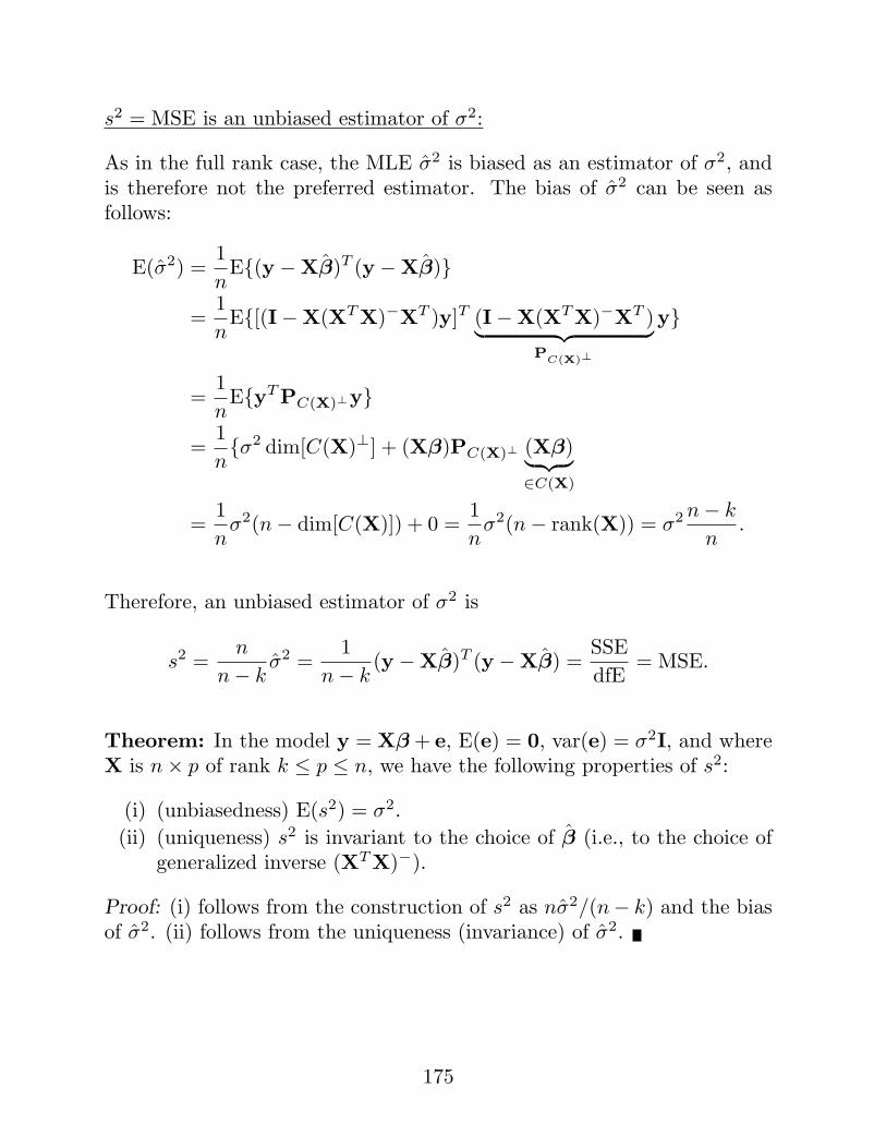
s2 = MSE is an unbiased estimator of σ2:

As in the full rank case, the MLE σ2 is biased as an estimator of σ2, andis therefore not the preferred estimator. The bias of σ2 can be seen asfollows:

E(σ2) =1n

E{(y −Xβ)T (y −Xβ)}

=1n

E{[(I−X(XT X)−XT )y]T (I−X(XT X)−XT )︸ ︷︷ ︸P

C(X)⊥

y}

=1n

E{yT PC(X)⊥y}

=1n{σ2 dim[C(X)⊥] + (Xβ)PC(X)⊥ (Xβ)︸ ︷︷ ︸

∈C(X)

=1n

σ2(n− dim[C(X)]) + 0 =1n

σ2(n− rank(X)) = σ2 n− k

n.

Therefore, an unbiased estimator of σ2 is

s2 =n

n− kσ2 =

1n− k

(y −Xβ)T (y −Xβ) =SSEdfE

= MSE.

Theorem: In the model y = Xβ + e, E(e) = 0, var(e) = σ2I, and whereX is n× p of rank k ≤ p ≤ n, we have the following properties of s2:

(i) (unbiasedness) E(s2) = σ2.(ii) (uniqueness) s2 is invariant to the choice of β (i.e., to the choice of

generalized inverse (XT X)−).

Proof: (i) follows from the construction of s2 as nσ2/(n− k) and the biasof σ2. (ii) follows from the uniqueness (invariance) of σ2.

175

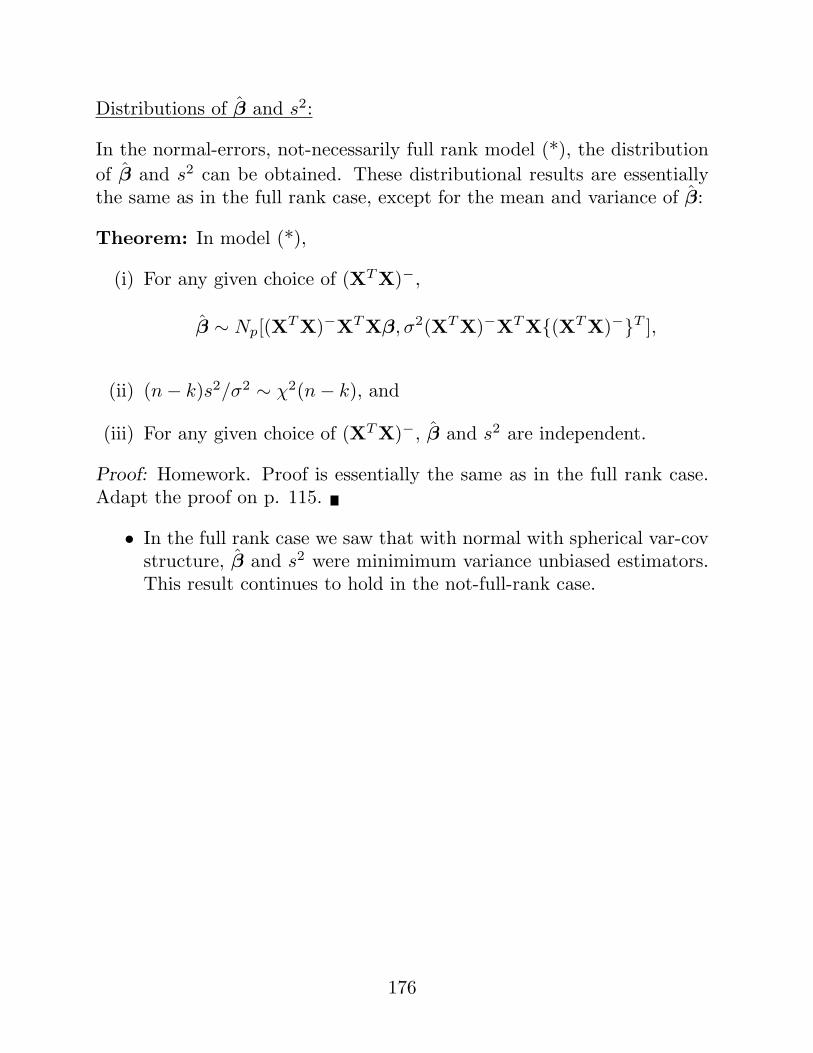
Distributions of β and s2:

In the normal-errors, not-necessarily full rank model (*), the distributionof β and s2 can be obtained. These distributional results are essentiallythe same as in the full rank case, except for the mean and variance of β:

Theorem: In model (*),

(i) For any given choice of (XT X)−,

β ∼ Np[(XT X)−XT Xβ, σ2(XT X)−XT X{(XT X)−}T ],

(ii) (n− k)s2/σ2 ∼ χ2(n− k), and

(iii) For any given choice of (XT X)−, β and s2 are independent.

Proof: Homework. Proof is essentially the same as in the full rank case.Adapt the proof on p. 115.

• In the full rank case we saw that with normal with spherical var-covstructure, β and s2 were minimimum variance unbiased estimators.This result continues to hold in the not-full-rank case.

176

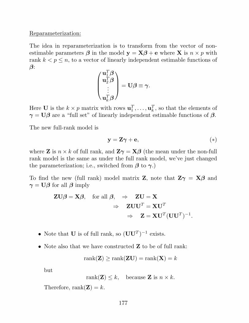
Reparameterization:

The idea in reparameterization is to transform from the vector of non-estimable parameters β in the model y = Xβ + e where X is n × p withrank k < p ≤ n, to a vector of linearly independent estimable functions ofβ:

uT1 β

uT2 β...

uTk β

= Uβ ≡ γ.

Here U is the k × p matrix with rows uT1 , . . . ,uT

k , so that the elements ofγ = Uβ are a “full set” of linearly independent estimable functions of β.

The new full-rank model is

y = Zγ + e, (∗)where Z is n× k of full rank, and Zγ = Xβ (the mean under the non-fullrank model is the same as under the full rank model, we’ve just changedthe parameterization; i.e., switched from β to γ.)

To find the new (full rank) model matrix Z, note that Zγ = Xβ andγ = Uβ for all β imply

ZUβ = Xβ, for all β, ⇒ ZU = X

⇒ ZUUT = XUT

⇒ Z = XUT (UUT )−1.

• Note that U is of full rank, so (UUT )−1 exists.

• Note also that we have constructed Z to be of full rank:

rank(Z) ≥ rank(ZU) = rank(X) = k

butrank(Z) ≤ k, because Z is n× k.

Therefore, rank(Z) = k.

177

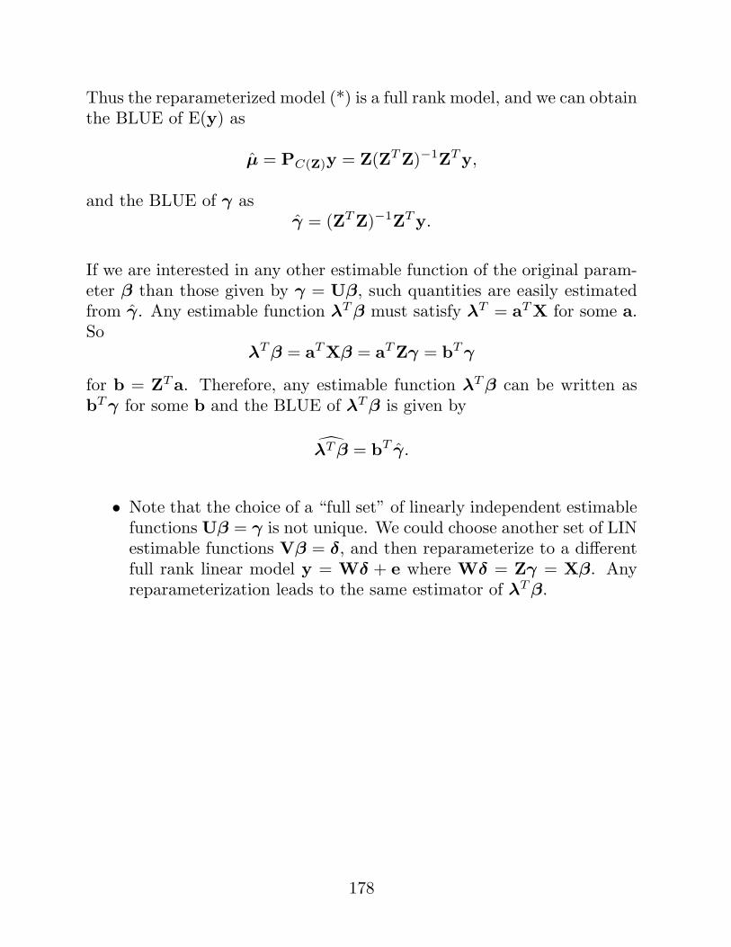
Thus the reparameterized model (*) is a full rank model, and we can obtainthe BLUE of E(y) as

µ = PC(Z)y = Z(ZT Z)−1ZT y,

and the BLUE of γ asγ = (ZT Z)−1ZT y.

If we are interested in any other estimable function of the original param-eter β than those given by γ = Uβ, such quantities are easily estimatedfrom γ. Any estimable function λT β must satisfy λT = aT X for some a.So

λT β = aT Xβ = aT Zγ = bT γ

for b = ZT a. Therefore, any estimable function λT β can be written asbT γ for some b and the BLUE of λT β is given by

λT β = bT γ.

• Note that the choice of a “full set” of linearly independent estimablefunctions Uβ = γ is not unique. We could choose another set of LINestimable functions Vβ = δ, and then reparameterize to a differentfull rank linear model y = Wδ + e where Wδ = Zγ = Xβ. Anyreparameterization leads to the same estimator of λT β.

178

Example: The Two-way ANOVA Model

In a two-way layout, observations are taken at all combinations of thelevels of two treatment factors. Suppose factor A has a levels and factor Bhas b levels, then in a balanced two-way layout n observations are obtainedin each of the ab treatments (combinations of A and B).

Let yijk = the kth observation at the ith level of A combined with the jth

level of B.

One way to think about the analysis of a two-way layout, is that if weignore factors A and B, then what we have is really just a one-way experi-ment with ab treatments. Therefore, a one-way layout-type model, with amean for each treatment can be used. This leads to the cell-means modelfor the two-way layout, which is a full-rank model:

yijk = µij + eijk, i = 1, . . . , a, j = 1, . . . , b, k = 1, . . . , n.

Often, an effects model is used instead for the two-way layout. In theeffects model, the (i, j)th treatment mean is decomposed into a constantterm plus additive effects for factor A, factor B, and factor A combinedwith factor B:

µij = µ + αi + βj + (αβ)ij

This leads to the effects model for the two-way layout:

yijk = µ + αi + βj + (αβ)ij + eijk, i = 1, . . . , a, j = 1, . . . , b, k = 1, . . . , n.

179

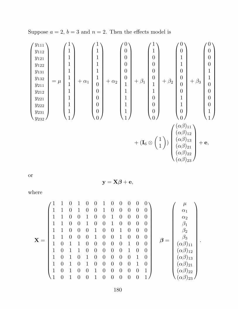
Suppose a = 2, b = 3 and n = 2. Then the effects model is

y111

y112

y121

y122

y131

y132

y211

y212

y221

y222

y231

y232

= µ

111111111111

+ α1

111111000000

+ α2

000000111111

+ β1

110000110000

+ β2

001100001100

+ β3

000011000011

+ (I6 ⊗(

11

))

(αβ)11(αβ)12(αβ)13(αβ)21(αβ)22(αβ)23

+ e,

ory = Xβ + e,

where

X =

1 1 0 1 0 0 1 0 0 0 0 01 1 0 1 0 0 1 0 0 0 0 01 1 0 0 1 0 0 1 0 0 0 01 1 0 0 1 0 0 1 0 0 0 01 1 0 0 0 1 0 0 1 0 0 01 1 0 0 0 1 0 0 1 0 0 01 0 1 1 0 0 0 0 0 1 0 01 0 1 1 0 0 0 0 0 1 0 01 0 1 0 1 0 0 0 0 0 1 01 0 1 0 1 0 0 0 0 0 1 01 0 1 0 0 1 0 0 0 0 0 11 0 1 0 0 1 0 0 0 0 0 1

β =

µα1

α2

β1

β2

β3

(αβ)11(αβ)12(αβ)13(αβ)21(αβ)22(αβ)23

.

180

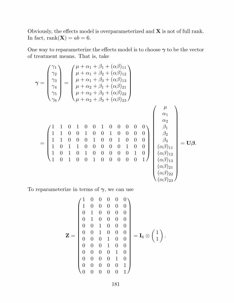
Obviously, the effects model is overparameterized and X is not of full rank.In fact, rank(X) = ab = 6.

One way to reparameterize the effects model is to choose γ to be the vectorof treatment means. That is, take

γ =

γ1

γ2

γ3

γ4

γ5

γ6

=

µ + α1 + β1 + (αβ)11µ + α1 + β2 + (αβ)12µ + α1 + β3 + (αβ)13µ + α2 + β1 + (αβ)21µ + α2 + β2 + (αβ)22µ + α2 + β3 + (αβ)23

=

1 1 0 1 0 0 1 0 0 0 0 01 1 0 0 1 0 0 1 0 0 0 01 1 0 0 0 1 0 0 1 0 0 01 0 1 1 0 0 0 0 0 1 0 01 0 1 0 1 0 0 0 0 0 1 01 0 1 0 0 1 0 0 0 0 0 1

µα1

α2

β1

β2

β3

(αβ)11(αβ)12(αβ)13(αβ)21(αβ)22(αβ)23

= Uβ.

To reparameterize in terms of γ, we can use

Z =

1 0 0 0 0 01 0 0 0 0 00 1 0 0 0 00 1 0 0 0 00 0 1 0 0 00 0 1 0 0 00 0 0 1 0 00 0 0 1 0 00 0 0 0 1 00 0 0 0 1 00 0 0 0 0 10 0 0 0 0 1

= I6 ⊗(

11

).

181

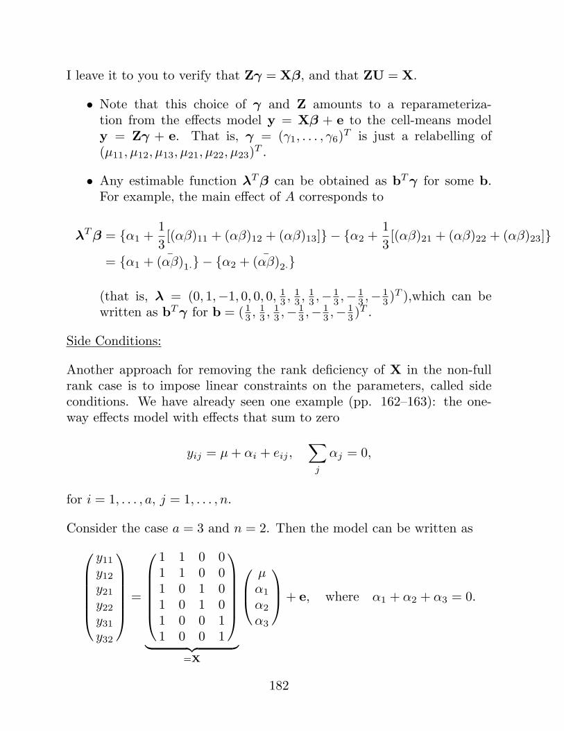
I leave it to you to verify that Zγ = Xβ, and that ZU = X.

• Note that this choice of γ and Z amounts to a reparameteriza-tion from the effects model y = Xβ + e to the cell-means modely = Zγ + e. That is, γ = (γ1, . . . , γ6)T is just a relabelling of(µ11, µ12, µ13, µ21, µ22, µ23)T .

• Any estimable function λT β can be obtained as bT γ for some b.For example, the main effect of A corresponds to

λT β = {α1 +13[(αβ)11 + (αβ)12 + (αβ)13]} − {α2 +

13[(αβ)21 + (αβ)22 + (αβ)23]}

= {α1 + ¯(αβ)1·} − {α2 + ¯(αβ)2·}

(that is, λ = (0, 1,−1, 0, 0, 0, 13 , 1

3 , 13 ,− 1

3 ,− 13 ,− 1

3 )T ),which can bewritten as bT γ for b = ( 1

3 , 13 , 1

3 ,− 13 ,− 1

3 ,− 13 )T .

Side Conditions:

Another approach for removing the rank deficiency of X in the non-fullrank case is to impose linear constraints on the parameters, called sideconditions. We have already seen one example (pp. 162–163): the one-way effects model with effects that sum to zero

yij = µ + αi + eij ,∑

j

αj = 0,

for i = 1, . . . , a, j = 1, . . . , n.

Consider the case a = 3 and n = 2. Then the model can be written as

y11

y12

y21

y22

y31

y32

=

1 1 0 01 1 0 01 0 1 01 0 1 01 0 0 11 0 0 1

︸ ︷︷ ︸=X

µα1

α2

α3

+ e, where α1 + α2 + α3 = 0.

182

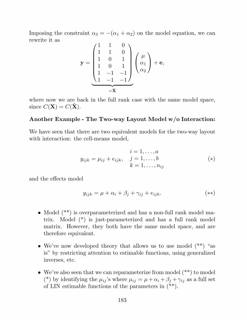
Imposing the constraint α3 = −(α1 + α2) on the model equation, we canrewrite it as

y =

1 1 01 1 01 0 11 0 11 −1 −11 −1 −1

︸ ︷︷ ︸=X

µα1

α2

+ e,

where now we are back in the full rank case with the same model space,since C(X) = C(X).

Another Example - The Two-way Layout Model w/o Interaction:

We have seen that there are two equivalent models for the two-way layoutwith interaction: the cell-means model,

yijk = µij + eijk,

i = 1, . . . , aj = 1, . . . , bk = 1, . . . , nij

(∗)

and the effects model

yijk = µ + αi + βj + γij + eijk. (∗∗)

• Model (**) is overparameterized and has a non-full rank model ma-trix. Model (*) is just-parameterized and has a full rank modelmatrix. However, they both have the same model space, and aretherefore equivalent.

• We’ve now developed theory that allows us to use model (**) “asis” by restricting attention to estimable functions, using generalizedinverses, etc.

• We’ve also seen that we can reparameterize from model (**) to model(*) by identifying the µij ’s where µij = µ+αi +βj +γij as a full setof LIN estimable functions of the parameters in (**).

183

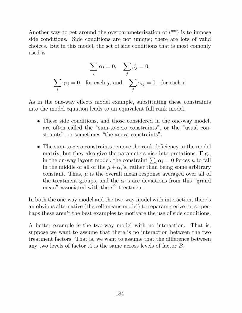
Another way to get around the overparameterization of (**) is to imposeside conditions. Side conditions are not unique; there are lots of validchoices. But in this model, the set of side conditions that is most comonlyused is

∑

i

αi = 0,∑

j

βj = 0,

∑

i

γij = 0 for each j, and∑

j

γij = 0 for each i.

As in the one-way effects model example, substituting these constraintsinto the model equation leads to an equivalent full rank model.

• These side conditions, and those considered in the one-way model,are often called the “sum-to-zero constraints”, or the “usual con-straints”, or sometimes “the anova constraints”.

• The sum-to-zero constraints remove the rank deficiency in the modelmatrix, but they also give the parameters nice interpretations. E.g.,in the on-way layout model, the constraint

∑i αi = 0 forces µ to fall

in the middle of all of the µ+αi’s, rather than being some arbitraryconstant. Thus, µ is the overall mean response averaged over all ofthe treatment groups, and the αi’s are deviations from this “grandmean” associated with the ith treatment.

In both the one-way model and the two-way model with interaction, there’san obvious alternative (the cell-means model) to reparameterize to, so per-haps these aren’t the best examples to motivate the use of side conditions.

A better example is the two-way model with no interaction. That is,suppose we want to assume that there is no interaction between the twotreatment factors. That is, we want to assume that the difference betweenany two levels of factor A is the same across levels of factor B.

184

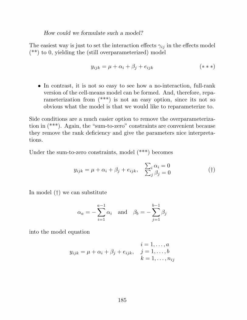
How could we formulate such a model?

The easiest way is just to set the interaction effects γij in the effects model(**) to 0, yielding the (still overparameterized) model

yijk = µ + αi + βj + eijk (∗ ∗ ∗)

• In contrast, it is not so easy to see how a no-interaction, full-rankversion of the cell-means model can be formed. And, therefore, repa-rameterization from (***) is not an easy option, since its not soobvious what the model is that we would like to reparameterize to.

Side conditions are a much easier option to remove the overparameteriza-tion in (***). Again, the “sum-to-zero” constraints are convenient becausethey remove the rank deficiency and give the parameters nice interpreta-tions.

Under the sum-to-zero constraints, model (***) becomes

yijk = µ + αi + βj + eijk,

∑i αi = 0∑j βj = 0 (†)

In model (†) we can substitute

αa = −a−1∑

i=1

αi and βb = −b−1∑

j=1

βj

into the model equation

yijk = µ + αi + βj + eijk,

i = 1, . . . , aj = 1, . . . , bk = 1, . . . , nij

185

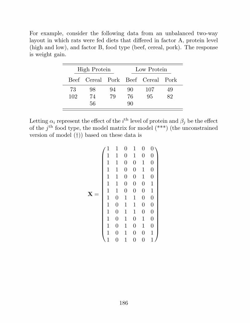
For example, consider the following data from an unbalanced two-waylayout in which rats were fed diets that differed in factor A, protein level(high and low), and factor B, food type (beef, cereal, pork). The responseis weight gain.

High Protein Low Protein

Beef Cereal Pork Beef Cereal Pork

73 98 94 90 107 49102 74 79 76 95 82

56 90

Letting αi represent the effect of the ith level of protein and βj be the effectof the jth food type, the model matrix for model (***) (the unconstrainedversion of model (†)) based on these data is

X =

1 1 0 1 0 01 1 0 1 0 01 1 0 0 1 01 1 0 0 1 01 1 0 0 1 01 1 0 0 0 11 1 0 0 0 11 0 1 1 0 01 0 1 1 0 01 0 1 1 0 01 0 1 0 1 01 0 1 0 1 01 0 1 0 0 11 0 1 0 0 1

186

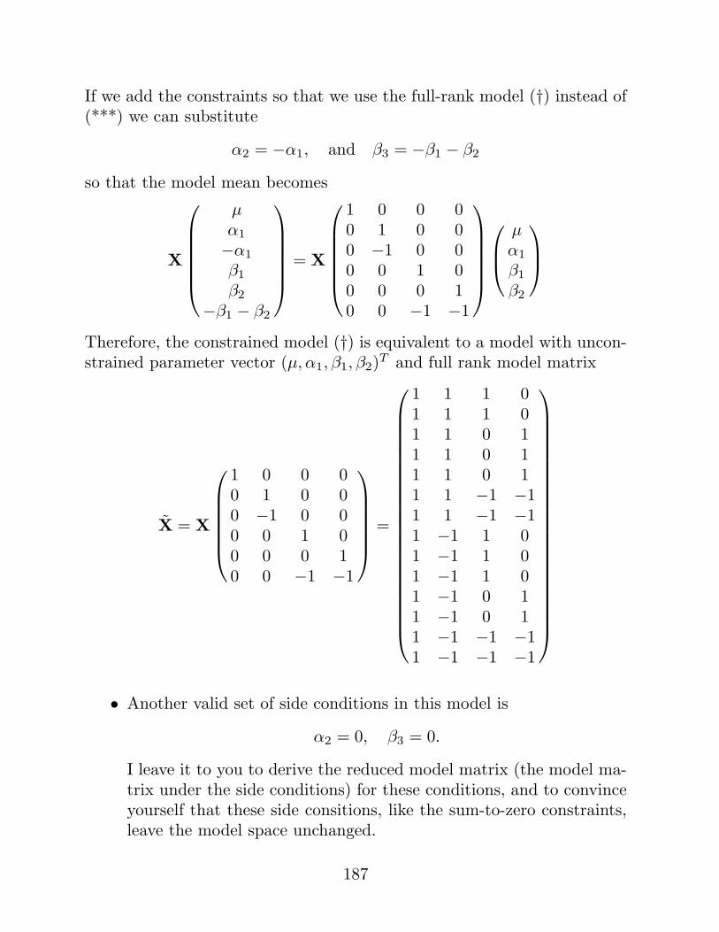
If we add the constraints so that we use the full-rank model (†) instead of(***) we can substitute

α2 = −α1, and β3 = −β1 − β2

so that the model mean becomes

X

µα1

−α1

β1

β2

−β1 − β2

= X

1 0 0 00 1 0 00 −1 0 00 0 1 00 0 0 10 0 −1 −1

µα1

β1

β2

Therefore, the constrained model (†) is equivalent to a model with uncon-strained parameter vector (µ, α1, β1, β2)T and full rank model matrix

X = X

1 0 0 00 1 0 00 −1 0 00 0 1 00 0 0 10 0 −1 −1

=

1 1 1 01 1 1 01 1 0 11 1 0 11 1 0 11 1 −1 −11 1 −1 −11 −1 1 01 −1 1 01 −1 1 01 −1 0 11 −1 0 11 −1 −1 −11 −1 −1 −1

• Another valid set of side conditions in this model is

α2 = 0, β3 = 0.

I leave it to you to derive the reduced model matrix (the model ma-trix under the side conditions) for these conditions, and to convinceyourself that these side consitions, like the sum-to-zero constraints,leave the model space unchanged.

187

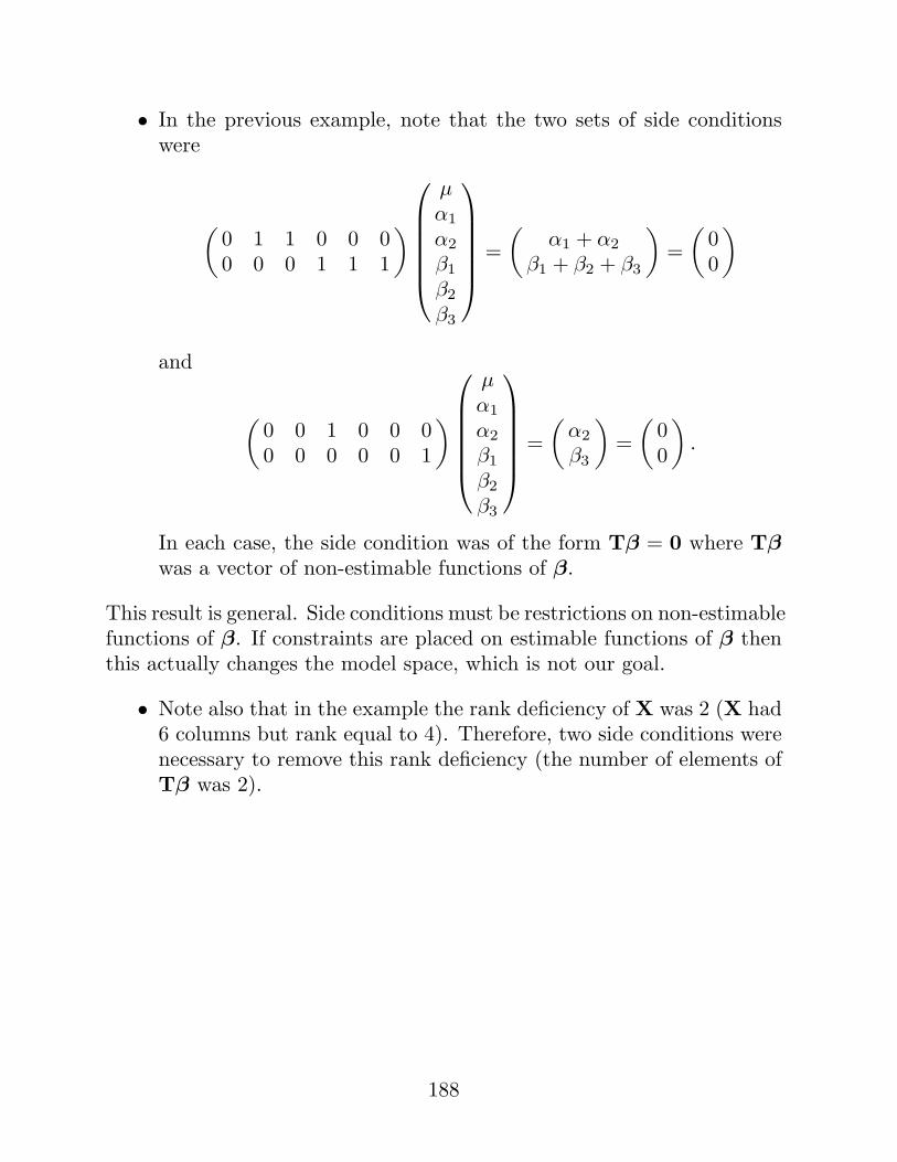
• In the previous example, note that the two sets of side conditionswere

(0 1 1 0 0 00 0 0 1 1 1

)

µα1

α2

β1

β2

β3

=(

α1 + α2

β1 + β2 + β3

)=

(00

)

and

(0 0 1 0 0 00 0 0 0 0 1

)

µα1

α2

β1

β2

β3

=(

α2

β3

)=

(00

).

In each case, the side condition was of the form Tβ = 0 where Tβwas a vector of non-estimable functions of β.

This result is general. Side conditions must be restrictions on non-estimablefunctions of β. If constraints are placed on estimable functions of β thenthis actually changes the model space, which is not our goal.

• Note also that in the example the rank deficiency of X was 2 (X had6 columns but rank equal to 4). Therefore, two side conditions werenecessary to remove this rank deficiency (the number of elements ofTβ was 2).

188

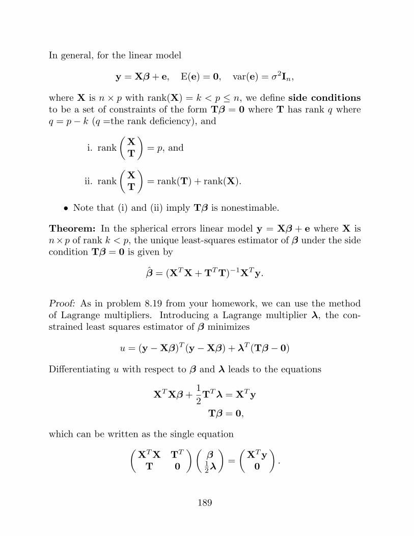
In general, for the linear model

y = Xβ + e, E(e) = 0, var(e) = σ2In,

where X is n × p with rank(X) = k < p ≤ n, we define side conditionsto be a set of constraints of the form Tβ = 0 where T has rank q whereq = p− k (q =the rank deficiency), and

i. rank(

XT

)= p, and

ii. rank(

XT

)= rank(T) + rank(X).

• Note that (i) and (ii) imply Tβ is nonestimable.

Theorem: In the spherical errors linear model y = Xβ + e where X isn×p of rank k < p, the unique least-squares estimator of β under the sidecondition Tβ = 0 is given by

β = (XT X + TT T)−1XT y.

Proof: As in problem 8.19 from your homework, we can use the methodof Lagrange multipliers. Introducing a Lagrange multiplier λ, the con-strained least squares estimator of β minimizes

u = (y −Xβ)T (y −Xβ) + λT (Tβ − 0)

Differentiating u with respect to β and λ leads to the equations

XT Xβ +12TT λ = XT y

Tβ = 0,

which can be written as the single equation(

XT X TT

T 0

)(β12λ

)=

(XT y

0

).

189

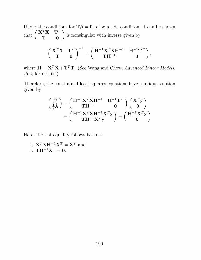
Under the conditions for Tβ = 0 to be a side condition, it can be shown

that(

XT X TT

T 0

)is nonsingular with inverse given by

(XT X TT

T 0

)−1

=(

H−1XT XH−1 H−1TT

TH−1 0

),

where H = XT X+TT T. (See Wang and Chow, Advanced Linear Models,§5.2, for details.)

Therefore, the constrained least-squares equations have a unique solutiongiven by

(β12 λ

)=

(H−1XT XH−1 H−1TT

TH−1 0

)(XT y

0

)

=(

H−1XT XH−1XT yTH−1XT y

)=

(H−1XT y

0

)

Here, the last equality follows because

i. XT XH−1XT = XT andii. TH−1XT = 0.

190

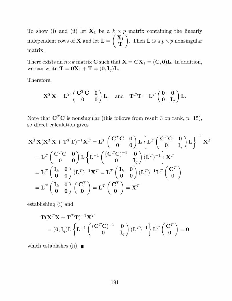
To show (i) and (ii) let X1 be a k × p matrix containing the linearly

independent rows of X and let L =(

X1

T

). Then L is a p×p nonsingular

matrix.

There exists an n×k matrix C such that X = CX1 = (C,0)L. In addition,we can write T = 0X1 + T = (0, Iq)L.

Therefore,

XT X = LT

(CT C 0

0 0

)L, and TT T = LT

(0 00 Iq

)L.

Note that CT C is nonsingular (this follows from result 3 on rank, p. 15),so direct calculation gives

XT X(XT X + TT T)−1XT = LT

(CT C 0

0 0

)L

{LT

(CT C 0

0 Iq

)L

}−1

XT

= LT

(CT C 0

0 0

)L

{L−1

((CT C)−1 0

0 Iq

)(LT )−1

}XT

= LT

(Ik 00 0

)(LT )−1XT = LT

(Ik 00 0

)(LT )−1LT

(CT

0

)

= LT

(Ik 00 0

)(CT

0

)= LT

(CT

0

)= XT

establishing (i) and

T(XT X + TT T)−1XT

= (0, Iq)L{L−1

((CT C)−1 0

0 Iq

)(LT )−1

}LT

(CT

0

)= 0

which establishes (ii).

191

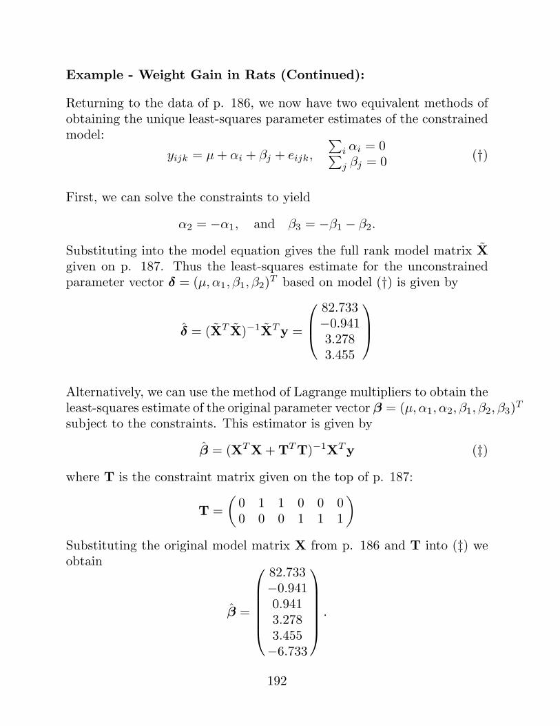
Example - Weight Gain in Rats (Continued):

Returning to the data of p. 186, we now have two equivalent methods ofobtaining the unique least-squares parameter estimates of the constrainedmodel:

yijk = µ + αi + βj + eijk,

∑i αi = 0∑j βj = 0 (†)

First, we can solve the constraints to yield

α2 = −α1, and β3 = −β1 − β2.

Substituting into the model equation gives the full rank model matrix Xgiven on p. 187. Thus the least-squares estimate for the unconstrainedparameter vector δ = (µ, α1, β1, β2)T based on model (†) is given by

δ = (XT X)−1XT y =

82.733−0.9413.2783.455

Alternatively, we can use the method of Lagrange multipliers to obtain theleast-squares estimate of the original parameter vector β = (µ, α1, α2, β1, β2, β3)T

subject to the constraints. This estimator is given by

β = (XT X + TT T)−1XT y (‡)where T is the constraint matrix given on the top of p. 187:

T =(

0 1 1 0 0 00 0 0 1 1 1

)

Substituting the original model matrix X from p. 186 and T into (‡) weobtain

β =

82.733−0.9410.9413.2783.455−6.733

.

192

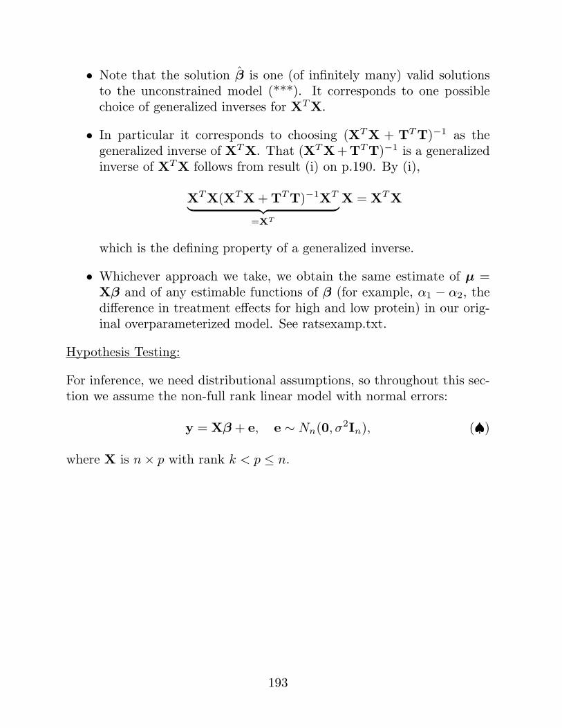
• Note that the solution β is one (of infinitely many) valid solutionsto the unconstrained model (***). It corresponds to one possiblechoice of generalized inverses for XT X.

• In particular it corresponds to choosing (XT X + TT T)−1 as thegeneralized inverse of XT X. That (XT X+TT T)−1 is a generalizedinverse of XT X follows from result (i) on p.190. By (i),

XT X(XT X + TT T)−1XT

︸ ︷︷ ︸=XT

X = XT X

which is the defining property of a generalized inverse.

• Whichever approach we take, we obtain the same estimate of µ =Xβ and of any estimable functions of β (for example, α1 − α2, thedifference in treatment effects for high and low protein) in our orig-inal overparameterized model. See ratsexamp.txt.

Hypothesis Testing:

For inference, we need distributional assumptions, so throughout this sec-tion we assume the non-full rank linear model with normal errors:

y = Xβ + e, e ∼ Nn(0, σ2In), (♠)

where X is n× p with rank k < p ≤ n.

193

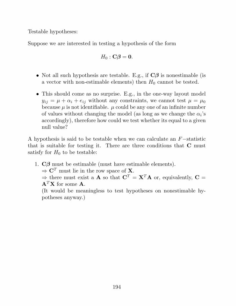
Testable hypotheses:

Suppose we are interested in testing a hypothesis of the form

H0 : Cβ = 0.

• Not all such hypothesis are testable. E.g., if Cβ is nonestimable (isa vector with non-estimable elements) then H0 cannot be tested.

• This should come as no surprise. E.g., in the one-way layout modelyij = µ + αi + eij without any constraints, we cannot test µ = µ0

because µ is not identifiable. µ could be any one of an infinite numberof values without changing the model (as long as we change the αi’saccordingly), therefore how could we test whether its equal to a givennull value?

A hypothesis is said to be testable when we can calculate an F−statisticthat is suitable for testing it. There are three conditions that C mustsatisfy for H0 to be testable:

1. Cβ must be estimable (must have estimable elements).⇒ CT must lie in the row space of X.⇒ there must exist a A so that CT = XT A or, equivalently, C =AT X for some A.(It would be meaningless to test hypotheses on nonestimable hy-potheses anyway.)

194

2. C must have full row rank. I.e., for C m×p, we require rank(C) = m.⇒ this ensures that the hypothesis contains no redundant state-ments.

– E.g., suppose β is 3 × 1 and we wish to test the hypothesisthat β1 = β2 = β3. We can express this hypothesis in the formH0 : Cβ for (infinitely) many choices of C. A valid choice ofC is

C =(

1 −1 00 1 −1

)

Notice that this 2× 3 matrix has row rank 2.

An invalid choice of C is

C =

1 −1 00 1 −11 0 −1

Notice that the last row is redundant (given that β1 = β2 andβ2 = β3 its redundant to require that β1 = β3), and rank(C) =2.

3. C must have no more than rank(X) = k rows.This is because, in general, one can only construct up to rank(X)linearly independent estimable functions.

Subject to these conditions, H0 is testable. As in the full rank case, thereare two equivalent approaches to testing H0:

1. Formulate a test statistic based on a comparison between Cβ andits null value 0.

2. Recast the null hypothesis H0 : Cβ = 0 in an equivalent form H0 :µ ∈ V0 for µ = E(y) = Xβ and an appropriate subspace V0 ⊂ V =C(X). That is, translate testing H0 into a full vs. reduced modeltesting problem.

• In the full rank case we described both of these approaches. Becauseof time constraints, we’ll only describe approach 1 in the non-fullrank case, but approach 2 follows in much the same way as before.

195

The General Linear Hypothesis:

As in the full rank case, our F test is based on the quadratic form

{Cβ − E0(Cβ)}T {var0(Cβ)}−1{Cβ − E0(Cβ)}= (Cβ)T {var0(Cβ)}−1(Cβ)

(Here the 0 subscript indicates that the expected value and variance arecomputed under H0 : Cβ = 0.)

The theorem leading to the F statistic is as follows:

Theorem: In model (♠), if C is m × p of rank m ≤ k = rank(X) suchthat Cβ is a set of m LIN estimable functions, and if β = GXT y, forsome generalized inverse G of XT X, then

(i) CGCT is nonsingular and invariant to the choice of G;

(ii) Cβ ∼ Nm(Cβ, σ2CGCT );

(iii) SSH/σ2 = (Cβ)T (CGCT )−1Cβ/σ2 ∼ χ2(m,λ), where

λ = (Cβ)T (CGCT )−1Cβ/(2σ2);

(iv) SSE/σ2 = yT (I−XGXT )y/σ2 ∼ χ2(n− k); and

(v) SSH and SSE are independent.

Proof:

(i) Since Cβ is a vector of estimable function, there must exist an A sothat C = AT X. Therefore,

CGCT = AT XGXT A = AT PC(X)A,

which is unique. To show CGCT is nonsingular we show that it isof full rank.

196

In general, we have the following two results about rank: (i) for anymatrix M, rank(MT M) = rank(MT ); and (ii) for any matrices Mand N, rank(MN) ≤ rank(M).

In addition, G can be chosen to be a symmetric generalized inverseof XT X (this is always possible), so G can be written G = LT L forsome L.

Therefore,

rank(CGCT ) = rank(CLT LCT ) = rank(CLT )

≥ rank(CLT L) = rank(CG) = rank(AT XG)

≥ rank(AT XGXT X) = rank(AT X) = rank(C) = m

So we’ve established that rank(CGCT ) ≥ m. But, since CGCT ism × m it follows that rank(CGCT ) ≤ m. Together, these resultsimply

rank(CGCT ) = m.

(ii) By the theorem on p. 176,

β ∼ Np[GXT Xβ, σ2GXT XG].

Therefore, Since Cβ is an affine transformation of a normal, andC = AT X for some A,

Cβ ∼ Nm[CGXT Xβ, σ2CGXT XGCT ]

= Nm[AT XGXT X︸ ︷︷ ︸=X

β, σ2AT XGXT X︸ ︷︷ ︸=X

GXT A]

= Nm(Cβ, σ2CGCT ].

197

(iii) By part (ii), var(Cβ) = σ2CGCT . Therefore, SSH/σ2 is a quadraticform in a normal random vector. Since,

σ2[CGCT ]−1CGCT /σ2 = I,

the result follows from the theorem on the bottom of p. 81.

(iv) This was established in part (ii) of the theorem on p. 176.

(v) Homework.

Putting the results of this theorem together, we obtain the F statistic fortesting H0 : Cβ = 0 for H0 a testable hypothesis:

Theorem: In the setup of the previous theorem, then the F statistic fortesting H0 : Cβ = 0 is as follows:

F =SSH/m

SSE/(n− k)

=(Cβ)T [CGCT ]−1Cβ/m

SSE/(n− k)∼ F (m,n− k, λ),

where G is a generalized inverse of XT X and

λ ={

12σ2 (Cβ)T (CGCT )−1(Cβ) in general0 under H0.

Proof: Follows directly from the previous theorem and the definition ofthe noncentral F distribution.

• As in the full rank case, this F statistic can be extended to test ahypothesis of the form H0 : Cβ = t for t a vector of constants,Cβ estimable, and C of full row rank. The resulting test statistic isidentical to F above, but with Cβ replaced by Cβ − t.

198

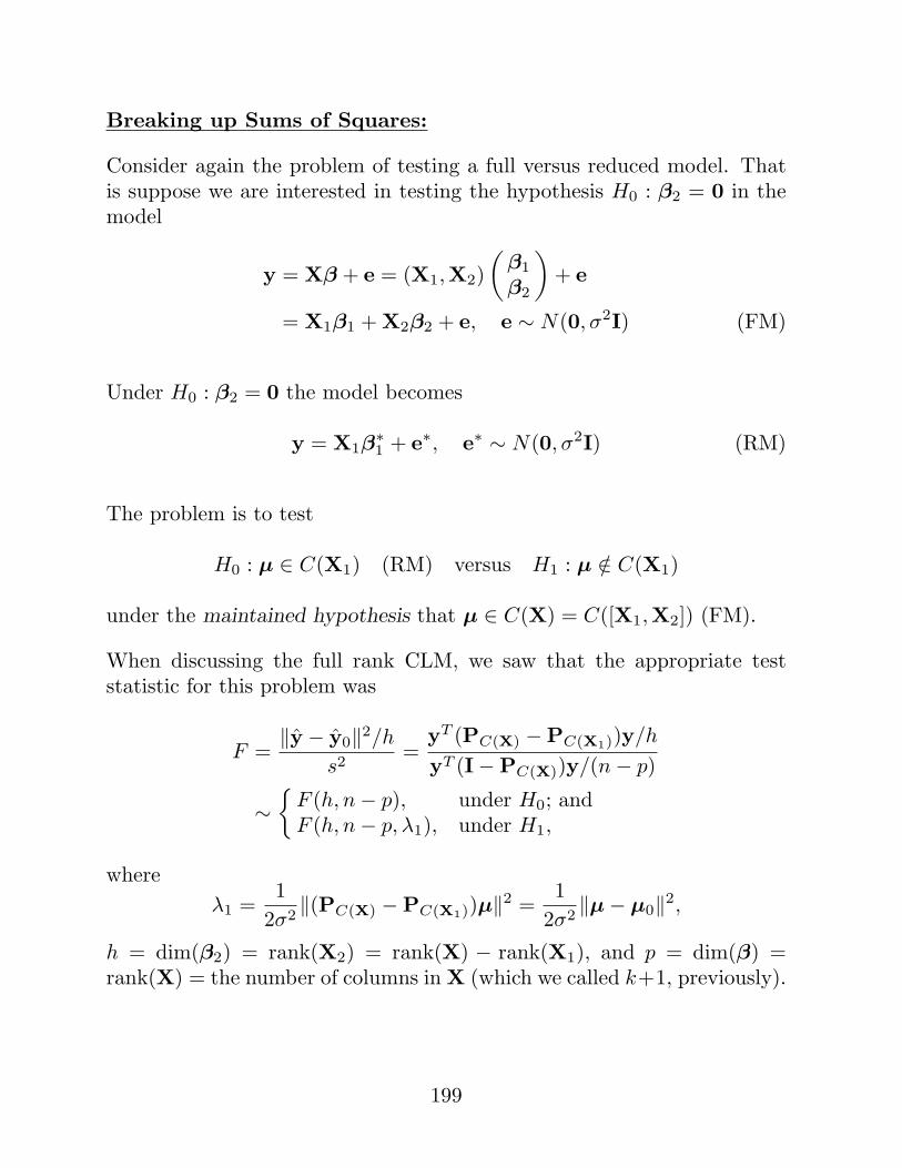
Breaking up Sums of Squares:

Consider again the problem of testing a full versus reduced model. Thatis suppose we are interested in testing the hypothesis H0 : β2 = 0 in themodel

y = Xβ + e = (X1,X2)(

β1

β2

)+ e

= X1β1 + X2β2 + e, e ∼ N(0, σ2I) (FM)

Under H0 : β2 = 0 the model becomes

y = X1β∗1 + e∗, e∗ ∼ N(0, σ2I) (RM)

The problem is to test

H0 : µ ∈ C(X1) (RM) versus H1 : µ /∈ C(X1)

under the maintained hypothesis that µ ∈ C(X) = C([X1,X2]) (FM).

When discussing the full rank CLM, we saw that the appropriate teststatistic for this problem was

F =‖y − y0‖2/h

s2=

yT (PC(X) −PC(X1))y/h

yT (I−PC(X))y/(n− p)

∼{

F (h, n− p), under H0; andF (h, n− p, λ1), under H1,

whereλ1 =

12σ2

‖(PC(X) −PC(X1))µ‖2 =1

2σ2‖µ− µ0‖2,

h = dim(β2) = rank(X2) = rank(X) − rank(X1), and p = dim(β) =rank(X) = the number of columns in X (which we called k+1, previously).

199

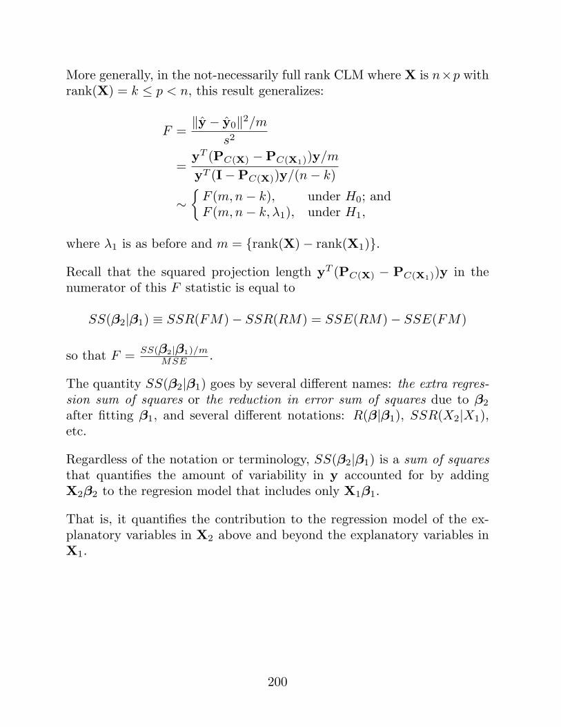
More generally, in the not-necessarily full rank CLM where X is n×p withrank(X) = k ≤ p < n, this result generalizes:

F =‖y − y0‖2/m

s2

=yT (PC(X) −PC(X1))y/m

yT (I−PC(X))y/(n− k)

∼{

F (m,n− k), under H0; andF (m,n− k, λ1), under H1,

where λ1 is as before and m = {rank(X)− rank(X1)}.

Recall that the squared projection length yT (PC(X) − PC(X1))y in thenumerator of this F statistic is equal to

SS(β2|β1) ≡ SSR(FM)− SSR(RM) = SSE(RM)− SSE(FM)

so that F = SS(β2|β1)/mMSE .

The quantity SS(β2|β1) goes by several different names: the extra regres-sion sum of squares or the reduction in error sum of squares due to β2

after fitting β1, and several different notations: R(β|β1), SSR(X2|X1),etc.

Regardless of the notation or terminology, SS(β2|β1) is a sum of squaresthat quantifies the amount of variability in y accounted for by addingX2β2 to the regresion model that includes only X1β1.

That is, it quantifies the contribution to the regression model of the ex-planatory variables in X2 above and beyond the explanatory variables inX1.

200

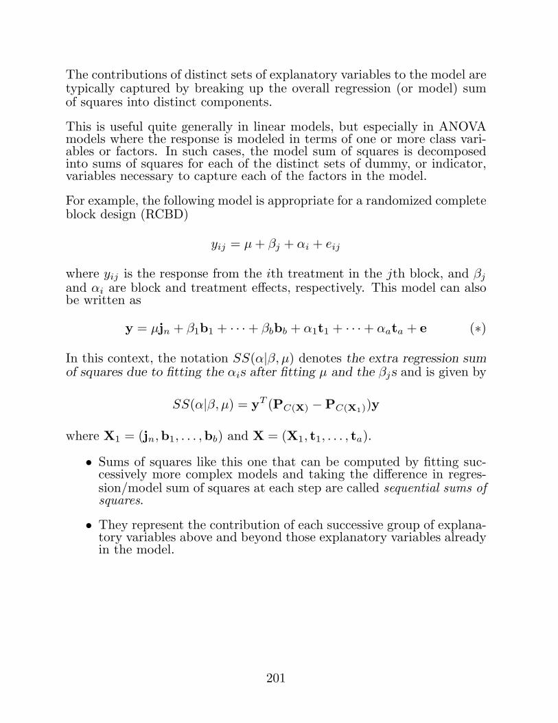
The contributions of distinct sets of explanatory variables to the model aretypically captured by breaking up the overall regression (or model) sumof squares into distinct components.

This is useful quite generally in linear models, but especially in ANOVAmodels where the response is modeled in terms of one or more class vari-ables or factors. In such cases, the model sum of squares is decomposedinto sums of squares for each of the distinct sets of dummy, or indicator,variables necessary to capture each of the factors in the model.

For example, the following model is appropriate for a randomized completeblock design (RCBD)

yij = µ + βj + αi + eij

where yij is the response from the ith treatment in the jth block, and βj

and αi are block and treatment effects, respectively. This model can alsobe written as

y = µjn + β1b1 + · · ·+ βbbb + α1t1 + · · ·+ αata + e (∗)

In this context, the notation SS(α|β, µ) denotes the extra regression sumof squares due to fitting the αis after fitting µ and the βjs and is given by

SS(α|β, µ) = yT (PC(X) −PC(X1))y

where X1 = (jn,b1, . . . ,bb) and X = (X1, t1, . . . , ta).

• Sums of squares like this one that can be computed by fitting suc-cessively more complex models and taking the difference in regres-sion/model sum of squares at each step are called sequential sums ofsquares.

• They represent the contribution of each successive group of explana-tory variables above and beyond those explanatory variables alreadyin the model.

201

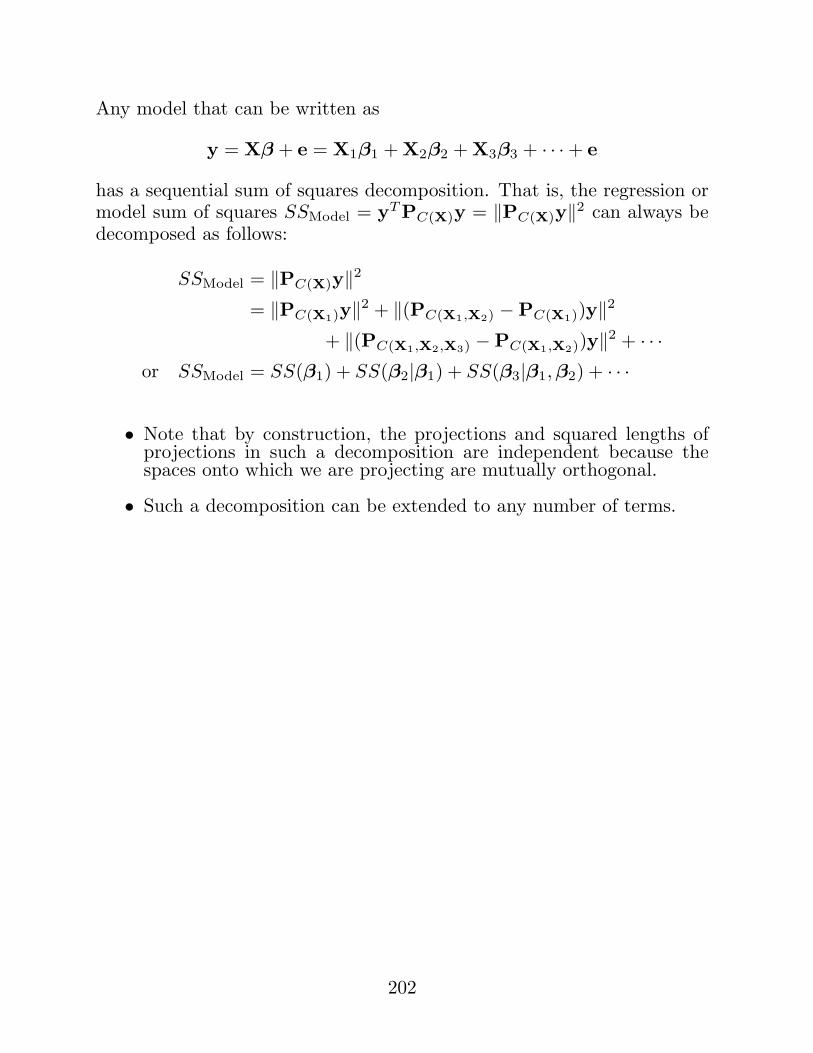
Any model that can be written as

y = Xβ + e = X1β1 + X2β2 + X3β3 + · · ·+ e

has a sequential sum of squares decomposition. That is, the regression ormodel sum of squares SSModel = yT PC(X)y = ‖PC(X)y‖2 can always bedecomposed as follows:

SSModel = ‖PC(X)y‖2= ‖PC(X1)y‖2 + ‖(PC(X1,X2) −PC(X1))y‖2

+ ‖(PC(X1,X2,X3) −PC(X1,X2))y‖2 + · · ·or SSModel = SS(β1) + SS(β2|β1) + SS(β3|β1, β2) + · · ·

• Note that by construction, the projections and squared lengths ofprojections in such a decomposition are independent because thespaces onto which we are projecting are mutually orthogonal.

• Such a decomposition can be extended to any number of terms.

202

Consider the RCBD model (*). This model can be written as

y = X1β1 + X2β2 + X3β3 + e

whereX1 = jN , X2 = (b1, . . . ,bb), X3 = (t1, . . . , ta)

and β1 = µ, β2 = (β1, . . . , βb)T , and β3 = (α1, . . . , αa)T .

The sequential break-down of the model sum of squares here is

SSModel = SS(µ) + SS(β|µ) + SS(α|β, µ) (∗∗)

Consider the null hypothesis H0 : α1 = · · · = αa = 0. The null modelcorresponding to this hypothesis is yij = µ + βj + eij .

Fitting just the null model we have

SSModel0 = SS(µ) + SS(β|µ).

Note that SSE = SST − SSModel, where SST = ‖y‖2 is the total (uncor-rected) sum of squares. Therefore, the difference in error sums of squaresbetween the null model and the maintained model is

SSE0 − SSE = (SST − SSModel0)− (SST − SSModel)

= SSModel − SSModel0 = SS(α|β, µ).

• That is, SS(α|β, µ) is an appropriate sum of squares for the nu-merator of the F− test for testing yij = µ + βj + eij versus yij =µ + βj + αi + eij .

• Similarly, we can test yij = µ + eij versus yij = µ + βj + eij usingSS(β|µ) as the numerator sum of squares.

• Finally, we can test yij = µ+ eij versus yij = µ+βj +αi + eij usingSS(α, β|µ) ≡ SS(α|β, µ) + SS(β|µ).

203

This last test is a test for significance of the entire model (other than theconstant term), or the overall regression test we have already encountered.

The sequential sums of squares used in decomposition (**) are known asType I sums of squares. This terminology is from SAS, but it has takenhold more generally.

Notice that with Type I (sequential) sums of squares we can decomposeSSModel either as

SSModel = SS(µ) + SS(β|µ) + SS(α|β, µ)

or asSSModel = SS(µ) + SS(α|µ) + SS(β|α, µ)

• That is, if we happen to add the block effects to the model first, thenthe appropriate test statistic is based on SS(α|β, µ). If we happento add the treatment effects first then the test is based on SS(α|µ).

• In addition, although SS(α|β, µ) = SS(α|µ) for some models (e.g.,balanced ANOVA models), such a result is not true, in general.

– Clearly, there’s something dissatisfying about obtaining differ-ent tests based on the order of the terms in the model.

– There’s an asymmetry in the way that the α’s and β’s aretreated in the Type I SSs.

• In contrast we might choose to always test the α’s based on SS(α|β, µ)and to test the β’s based on SS(β|α, µ).

• Sums of squares like SS(α|β, µ) and SS(β|α, µ) are called Type IIsums of squares in SAS.

204

• Type II SS’s correct the order-dependence of Type I SS’s. In theRCBD mode, for example, Type II SS’s treat main effects for blocks(SS(β|α, µ)) and treatments (SS(α|β, µ)) in a symmetric way.

• For a full definition of Type II SS’s we need to understand what ahierarchical model is.

Hierarchical models: Hierarchical models are models in which the in-clusion of any interaction effect necessarily implies the inclusion of alllower-level interactions and main effects involving the factors of the origi-nal interaction.

• E.g., in the context of a two-way layout, the usual model has maineffects αi and βj for the levels of each of the two factors A and B, andinteraction effects (αβ)ij corresponding to A ∗B. However, there isnothing to prevent us from considering simpler models.

• The modelyijk = µ + αi + (αβ)ij + eijk

is not a hierachical model, because we have included an A ∗B inter-action, but no main effect for factor B. In a hierarchical model, theinclusion of (αβ)ij requires the inclusion of both αi and βj .

• Similarly, suppose we have a three-way layout. The full hierarchicalmodel is

yijkl = µ+αi +βj + γk +(αβ)ij +(αγ)ik +(βγ)jk +(αβγ)ijk + eijkl

Here, γk is an effect for the kth level of factor C, (αγ)ik and (βγ)jk

are two way interactions for A ∗ C and B ∗ C, and (αβγ)ijk is thethree-way interaction A ∗ B ∗ C. Two examples of non-hierarchicalthree-factor models are

yijkl = µ + αi + βj + γk + (αβ)ij + (βγ)jk + (αβγ)ijk + eijkl

and yijkl = µ + αi + γk + (αβ)ij + (αγ)ik + (αβγ)ijk + eijkl

205

• I believe (and most statisticians would agree) that, in general, itis best to restrict attention to hierarchical models unless there is acompelling reason that in a particular application the omission of alower-order term makes sense (e.g., is suggested by some theory orknown fact from the context of the problem).

– This principle is similar to the notion that in a polynomialregression model: yi = β0 + β1xi + β2x

2i + · · · + βqx

qi + ei

one should not consider any model in which a term βkxki is

included, but where any of the terms β0, β1xi, . . . , βk−1xk−1i

are excluded.

Type II SS’s computes the SS for a factor U , say, as the reduction in SS’sobtained by adding a term for factor U to the model that is the largesthierarchical model that does not contain U .

• E.g., in the two-way layout, the Type II SS’s are

SSA = SS(α|β, µ), SSB = SS(β|α, µ), SSAB = SS((αβ)|α, β, µ)

– Notice that there is no longer an order effect. Factor B isadjusted for A and factor A is adjusted for B.

• Another example: in the three-way layout, the Type II SS’s are

SSA = SS(α|µ, β, γ, (βγ)), SSB = SS(β|µ, α, γ, (αγ)), SSC = SS(γ|µ, α, β, (αβ))SSAB = SS((αβ)|µ, α, β, γ, (αγ), (βγ)) SSAC = SS((αγ)|µ, α, β, γ, (αβ), (βγ))SSBC = SS((βγ)|µ, α, β, γ, (αβ), (αγ)) SSABC = SS((αβγ)|µ, α, β, γ, (αβ), (αγ), (βγ))

206

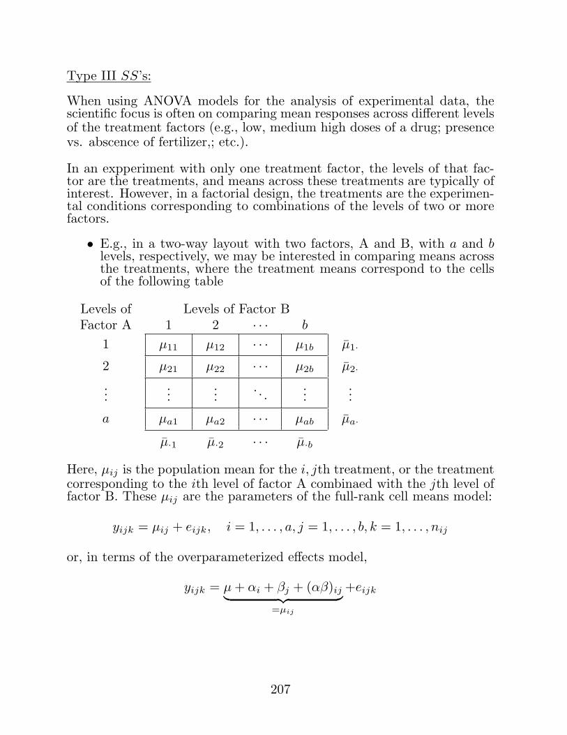
Type III SS’s:

When using ANOVA models for the analysis of experimental data, thescientific focus is often on comparing mean responses across different levelsof the treatment factors (e.g., low, medium high doses of a drug; presencevs. abscence of fertilizer,; etc.).

In an expperiment with only one treatment factor, the levels of that fac-tor are the treatments, and means across these treatments are typically ofinterest. However, in a factorial design, the treatments are the experimen-tal conditions corresponding to combinations of the levels of two or morefactors.

• E.g., in a two-way layout with two factors, A and B, with a and blevels, respectively, we may be interested in comparing means acrossthe treatments, where the treatment means correspond to the cellsof the following table

Levels of Levels of Factor BFactor A 1 2 · · · b

1 µ11 µ12 · · · µ1b µ1·

2 µ21 µ22 · · · µ2b µ2·...

......

. . ....

...

a µa1 µa2 · · · µab µa·

µ·1 µ·2 · · · µ·b

Here, µij is the population mean for the i, jth treatment, or the treatmentcorresponding to the ith level of factor A combinaed with the jth level offactor B. These µij are the parameters of the full-rank cell means model:

yijk = µij + eijk, i = 1, . . . , a, j = 1, . . . , b, k = 1, . . . , nij

or, in terms of the overparameterized effects model,

yijk = µ + αi + βj + (αβ)ij︸ ︷︷ ︸=µij

+eijk

207

While it is often of interest to compare treatment means (e.g., to testH0 : µij = µi′j′), it also often of interest to compare the mean responseacross levels of factor A marginally; that is, after averaging across factorB (or vice versa).

We define the marginal mean at the ith level of factor A to be µi· =1b

∑bj=1 µij or, in terms of the effects model,

µi· =1b

b∑

j=1

(µ + αi + βj + (αβ)ij) = µ + αi + β· + ¯(αβ)i·.

• Marginal means for each of the level of factor B are defined similarly.

If we are interested in making comparisons among the marginal means, itwould be nice if our sum of squares for factor A, and for factor B led toan F test, F = SSA/dfA

MSE , which tested a simple hypothesis of interest likeH0 : µ1· = µ2· = · · · = µa·.

• It turns out that both the Type I and Type II approach to calculatingSSA do not test such a hypothesis. Type III SS’s, also know asmarginal sums of squares, do.

It can be shown that, in terms of the marginal means, the hypothesestested by Type I and Type II SS’s are difficult to interpret, and not atall the sorts of hypotheses that one would typically be interested in if thefocus of the analysis was to compare treatment means (which it usuallyis).

208

• For example, in the two-way layout, the hypotheses tested by FA =SSA/dfA

MSEfor Type I and II versions of SSA are:

Type I: H0 :b∑

j=1

n1jµ1j

n1·= · · · =

b∑

j=1

najµaj

na·

Type II: H0 :b∑

j=1

n1jµ1j =a∑

i=1

b∑

j=1

n1jnijµij

n·j, . . . ,

b∑

j=1

najµaj =a∑

i=1

b∑

j=1

najnijµij

n·j

• These hypotheses (especially those from Type II) are strange. Theycorrespond to testing whether certain weighted marginal averages ofthe treatment means are equal. Testing such hypotheses is seldomof interest. If one is interested in comparing means across the levelsof factor A, these SS’s are definitely not what one would want touse.

Type III SS’s are designed to always test simple hypotheses on (un-weighted) marginal population means. In particular, for the Type IIIversion of SSA, FA tests the hypothesis

Type III: H0 : µ1· = · · · = µa·

Similarly, the Type III version of SSB leads to a test of

Type III: H0 : µ·1 = · · · = µ·b

• All three types of SS’s lead to the same (reasonable and appropriate)hypothesis for FAB = MSAB/MSE . Namely,

H0 : (µij − µij′)− (µi′j − µi′j′) = 0, for all i, i′, j, j′

209

Type III SS’s also have an interpretation in terms of reduction in SS’s.For the two way layout model with sum-to-zero restrictions on theparameters the Type III SS’s are:

SSA = SS(α|µ, β, (αβ)), SSB = SS(β|µ, α, (αβ)), SSAB = SS((αβ)|µ, α, β).

• Note that this interpretation only applies to the sum-to-zero re-stricted version of the two-way layout model. For other restrictions,the interpretation would be different. A much better way to un-derstand Type III SS’s is in terms of the hypotheses tested on themarginal means, as described above.

Type IV SS’s:

The fourth type of SS’s is useful when there are certain treatment combi-nations for which nij = 0.

• My recommendation is to avoid the use of Type IV SSs. If factorialdesigns are encountered with missing treatments, I suggest insteadthe use of a one-way anova model, treating the treatments with dataas levels of a single treatment factor. Interactions and main effectscan be investigated by testing hypotheses on the treatment means.

• If you’re really interested, you can refer to Milliken & Johnson (1992)or Littell, Freund, & Spector (SAS System for Linear Models, ThirdEdition, 1991) for information on Type IV SS’s.

210

Relationships Among the Types and Recommendations:

In certain situations, the following equalities among the types of SS’s hold:

I = II = III = IV for balanced data

II = III = IV for no-interaction models

III = IV for all-cells-filled data

If one is interested in model-building (finding a parsimonious well-fittingmodel for the data) then

i. use Type I for choosing between models of sequentially increasingcomplexity; and

ii. use Type II for choosing between hierarchical models.

If one is interested in testing hypotheses that compare means across thelevels of experimentally controlled factors

iii. use Type III.

• Note that Type I SS’s are the only type of sum of squares that, ingeneral, lead decompose the total sum of squares. E.g., in the two-way anova model, they are the only type of SS that guarantee thatSST = SSA + SSB + SSAB + SSE holds, in general.

• However, all four types yield sums of squares that are independentof SSE and all lead to valid F tests (just of different hypotheses).

• Independence of these SSs from the SSE is guaranteed because allfour types of SSs are squared lengths of projections onto some sub-space of C(X), whereas SSE is the squared length of a projectiononto C(X)⊥.

211