Embed Size (px)
Citation preview

PARAMETRIC FEYNMAN INTEGRALS AND DETERMINANT
HYPERSURFACES
PAOLO ALUFFI AND MATILDE MARCOLLI
Abstract. The purpose of this note is to show that, under certain combinatorialconditions on the graph, parametric Feynman integrals can be realized as periods on
the complement of the determinant hypersurface Dℓ in affine space Aℓ2 , with ℓ thenumber of loops of the Feynman graph. The question of whether these are periods ofmixed Tate motives can then be reformulated as a question on a relative cohomology
of the pair (Aℓ2 r Dℓ, Σℓ,g r (Σℓ,g ∩ Dℓ)) being a realization of a mixed Tate motive,
where Σℓ,g is a normal crossings divisor depending only on the number of loops and thegenus of the graph. We show explicitly that the relative cohomology is a realization ofa mixed Tate motive in the case of three loops and we give alternative formulations of
the main question in the general case by describing the locus Σℓ,g r(Σℓ∩Dℓ)) in termsof intersections of unions of Schubert cells in flag varieties. We also discuss differentmethods of regularization aimed at removing the divergences of the Feynman integral.
1. Introduction
The question of whether Feynman integrals arising in perturbative scalar quantum fieldtheory are periods of mixed Tate motives can be seen (see [10], [9]) as a question on whethercertain relative cohomologies associated to algebraic varieties defined by the data of theparametric representation of the Feynman integral are realizations of mixed Tate motives.In this paper we investigate another possible viewpoint on the problem, which leads us toconsider a different relative cohomology, defined in terms of the complement of the affinedeterminant hypersurface and the locus where the hypersurface intersects the image of asimplex under a linear map defined by the Feynman graph. For all graphs with a givennumber of loops ℓ, admitting a minimal embedding in an orientable surface of genus g,and satisfying a natural combinatorial condition, we relate the question mentioned aboveto a problem in the geometry of coordinate subspaces of an ℓ-dimensional vector space,which only depends on the genus g. More precisely we first show that, modulo the issueof divergences, for certain classes of graphs identified by combinatorial conditions, the
parametric Feynman integral is a period of the pair (Aℓ2 r Dℓ, Σℓ,g r (Dℓ ∩ Σℓ,g), where
Aℓ2 r Dℓ is the complement of the determinant hypersurface Dℓ in the affine space Aℓ2 ,
while Σℓ,g is a normal crossings divisor in Aℓ2 that only depends on the number of loops ℓand on the genus g. We then show that, therefore, the question of whether the Feynmanintegrals are periods of mixed Tate motives becomes a question about the whether themotive
m(Aℓ2 r Dℓ, Σℓ,g r (Dℓ ∩ Σℓ,g))
whose realization is the relative cohomology of the pair, is in fact mixed Tate. We showthat, using inclusion-exclusion, the question for different graphs with the same genus andnumber of loops reduces to subsets of components of the same divisor Σℓ,g. We solve
the problem for ℓ ≤ 3 loops, by showing that the motive m(A9 r D3, Σ3,0 r (D3 ∩ Σ3,0)is mixed Tate, by constructing explicit filtrations. We also obtain in this case explicitformulae for the class [Σ3,0 r (D3 ∩ Σ3,0)] in the Grothendieck group, for the case of Σ3,0
1

2 ALUFFI AND MARCOLLI
itself and of all subsets of its components, which are used to construct the divisors ΣΓ
for all graphs with 3-loops. We discuss the problem in general terms for arbitrary ℓ, givedifferent formulations, and list conditions that would be sufficient to imply the desiredresult. Finally, we discuss the problem of regularization of divergent Feynman integrals,and how different possible regularizations can be made compatible with the approach viadeterminant hypersurfaces described here.
We recall the basic notation and terminology we use in the following.
Definition 1.1. Consider a scalar field theory with Lagrangian
(1.1) L(φ) =1
2(∂φ)2 −
m2
2φ2 − Lint(φ),
where Lint(φ) is a polynomial in φ of degree at least three. Then a one particle irre-ducible (1PI) Feynman graph Γ of the theory is a finite connected graph with the followingproperties.
• The valence of each vertex is equal to the degree of one of the monomials in theLagrangian (1.1).
• The set E(Γ) of edges of the graph is divided into internal and external edges,E(Γ) = Eint(Γ) ∪ Eext(Γ). Each internal edge connects two vertices of the graph,while the external edges have only one vertex. (One thinks of an internal edges asbeing a union of two half-edges and an external one as being a single half-edge.)
• The graph cannot be disconnected by removing a single internal edge. This is the1PI condition.
In the following we denote by n = #Eint(Γ) the number of internal edges, by N =#Eext(Γ) the number of external edges, and by ℓ = b1(Γ) the number of loops.
In their parametric form, the Feynman integrals of massless perturbative scalar quan-tum field theories (cf. §6-2-3 of [22], §18 of [7], and §6 of [27]) are integrals of the form
(1.2) U(Γ, p) =Γ(n − Dℓ/2)
(4π)ℓD/2
∫
σn
PΓ(t, p)−n+Dℓ/2 ωn
ΨΓ(t)−n+(ℓ+1)D/2,
where Γ(n − Dℓ/2) is a possibly divergent Γ-factor, σn is the simplex
(1.3) σn = {(t1, . . . , tn) ∈ Rn+ |
∑
i
ti = 1}
and the polynomials ΨΓ(t) and PΓ(t, p) are obtained from the combinatorics of the graph,respectively as
(1.4) ΨΓ(t) =∑
T⊂Γ
∏
e/∈E(T )
te,
where the sum is over all the spanning trees T of Γ and
(1.5) PΓ(p, t) =∑
C⊂Γ
sC
∏
e∈C
te,
where the sum is over the cut-sets C ⊂ Γ, i.e. the collections of b1(Γ) + 1 internal edgesthat divide the graph Γ in exactly two connected components Γ1 ∪ Γ2. The coefficient sC
is a function of the external momenta attached to the vertices in either one of the twocomponents
(1.6) sC =
∑
v∈V (Γ1)
Pv
2
=
∑
v∈V (Γ2)
Pv
2
.
FEYNMAN INTEGRALS AND DETERMINANTS 3
Here the Pv are defined as
(1.7) Pv =∑
e∈Eext(Γ),t(e)=v
pe,
where the pe are incoming external momenta attached to the external edges of Γ andsatisfying the conservation law
(1.8)∑
e∈Eext(Γ)
pe = 0.
In order to work with algebraic differential forms defined over Q, we assume that theexternal momenta are also taking rational values pe ∈ QD.
Ignoring the Γ-function factor in (1.2), one is interested in understanding what kind ofperiod is the integral
(1.9)
∫
σn
PΓ(t, p)−n+Dℓ/2 ωn
ΨΓ(t)−n+(ℓ+1)D/2.
In quantum field theory one can consider the same physical theory (with specifiedLagrangian) in different spacetime dimensions D ∈ N. In fact, one should think of thedimension D as one of the variable parameters in the problem. For the purposes of thispaper, we work in the range where D is sufficiently large, so that n ≤ Dℓ/2. The casen = Dℓ/2 is the log divergent case, where the integral (1.9) simplifies to the form
(1.10)
∫
σn
ωn
ΨΓ(t)D/2.
Another case where the Feynman integral has the simpler form (1.10), even for graphsthat do not necessarily satisfy the log divergent condition, i.e. for n 6= Dℓ/2, is where oneconsiders the case with nonzero mass m 6= 0, but with external momenta set equal to zero.In such cases, the parametric Feynman integral becomes of the form
(1.11)
∫
σn
VΓ(t, p)−n+Dℓ/2ωn
ΨΓ(t)D/2|p=0 = m−2n+Dℓ
∫
σn
ωn
ΨΓ(t)D/2,
where VΓ(t, p) is of the form
VΓ(t, p) = p†RΓ(t)p + m2,
with
VΓ(t, p)|m=0 =PΓ(t, p)
ΨΓ(t).
In the following we assume that we are either in the massless case (1.9) and in the rangeof dimensions D satisfying n ≤ Dℓ/2, or in the massive case with zero external momenta(1.11) and arbitrary dimension.
A first issue one needs to clarify in addressing the question of Feynman integrals andperiods is the fact that the integral (1.9) is often divergent. Divergences are contributed
by the intersection σn ∩ XΓ, with XΓ = {t ∈ An |ΨΓ(t) = 0}, which is often non-empty.
Although there are cases where a nonempty intersection σn ∩ XΓ may still give rise to anabsolutely convergent integral, hence a period, these are relatively rare cases and usuallysome regularization and renormalization procedure is needed to eliminate the divergencesover the locus where the domain of integration meets the graph hypersurface. Noticethat these intersections only occur on the boundary ∂σn, since in the interior of σn thepolynomial ΨΓ(t) is strictly positive (see (1.4)).
Our results will apply directly to all cases where the integral is convergent, while wediscuss in Section 7 the case where a regularization procedure is required to treat diver-gences in the Feynman integrals. The main question is then, more precisely formulated,

4 ALUFFI AND MARCOLLI
whether it is true that the numbers obtained by computing such integrals (after removinga possibly divergent Gamma factor, and after regularization and renormalization whenneeded) are always periods of mixed Tate motives. While we are unable to answer thequestion at this point, we give a reformulation of the problem, where instead of workingwith the graph hypersurfaces XΓ defined by the vanishing of the graph polynomial ΨΓ,one works with the complement of determinant hypersurfaces, and the problem is reducedto a question that only depends on the number of loops ℓ of the graph and on its genus g(see §3). If this question is answered affirmatively for a pair (ℓ, g), it follows that all graphsof genus g with ℓ loops, and satisfying the combinatorial condition discussed in §2 (forexample, all 3-vertex connected planar graphs with ℓ loops), can only produce periods ofmixed Tate motives.
This question is expressed in terms of the complement of the determinant hypersurface
in a normal crossing divisor Σℓ,g in the space Aℓ2 of ℓ × ℓ matrices. Precise questions interms of ℓ alone are formulated in §5.3; these questions may be appreciated independentlyof our motivation, as they do not refer directly to Feynman graphs. We hope that thesereformulations might help to connect the problem to other interesting questions, such asthe geometry of intersections of Schubert cells and Kazhdan–Lusztig theory.
In this paper (§6) we offer a completely explicit and elementary affirmative answer toour question for ℓ ≤ 3.
2. Feynman parameters and determinants
With the notation as above, for a given Feynman graph Γ, the graph hypersurface XΓ
is defined as the locus of zeros
(2.1) XΓ = {t = (t1 : . . . : tn) ∈ Pn−1 |ΨΓ(t) = 0}.
Indeed, ΨΓ is homogeneous of degree ℓ, hence it defines a hypersurface of degree ℓ in theprojective space Pn−1. We will also consider the affine cone on XΓ, namely the affinehypersurface
(2.2) XΓ = {t ∈ An |ΨΓ(t) = 0}.
The question of whether the Feynman integral is a period of a mixed Tate motive canbe approached (modulo the divergence problem) as a question on whether the relativecohomology
(2.3) Hn−1(Pn−1 r XΓ, Σn r (Σn ∩ XΓ))
is a realization of a mixed Tate motive, where Σn is the algebraic simplex
(2.4) Σn = {t ∈ Pn−1 |∏
i
ti = 0},
i.e. the union of the coordinate hyperplanes containing the boundary of the domain ofintegration ∂σn ⊂ Σn. See for instance [10], [9].
Although working in the projective setting is very natural (see [10]), there are severalreasons why it may be preferable to consider affine hypersurfaces:
• Only in the limit cases of a massless theory or of zero external momenta in themassive case does the parameteric Feynman integral involve the quotient of twohomogeneous polynomial ([7], §18).
• The deformations of the φ4 quantum field theory to noncommutative spacetime,which has been the focus of much recent research (see e.g. [20]), shows that, even inthe massless case the graph polynomials ΨΓ and PΓ are no longer homogeneous inthe noncommutative setting and only in the limit commutative case they recoverthis property (see [21], [23]).
FEYNMAN INTEGRALS AND DETERMINANTS 5
• As shown in [2], in the affine setting the graph hypersurface complement satisfiesa multiplicative property over disjoint unions of graphs that makes it possible todefine algebro-geometric and motivic Feynman rules.
For these various reasons, in this paper we primarily work in the affine rather than in theprojective setting.
In the present paper, we approach the problem in a different way, where instead ofworking with the hypersurface XΓ, we map the Feynman integral computation and thegraph hypersurface in a larger hypersurface Dℓ inside a larger affine space, so that wewill be dealing with a relative cohomology replacing (2.3) where the ambient space (thehypersurface complement) only depends on the number of loops in the graph.
2.1. Determinant hypersurfaces and graph polynomials. We now show that all theaffine varieties XΓ, for fixed number of loops ℓ, map naturally to a larger hypersurface ina larger affine space, by realizing the polynomial ΨΓ for the given graph as a pullback ofa fixed polynomial Ψℓ in ℓ2-variables.
Recall that the determinant hypersurface Dℓ is defined in the following way. Letk[xkr , k, r = 1, . . . , ℓ] be the polynomial ring in ℓ2 variables and set
(2.5) Dℓ = {x = (xkr) | det(x) = 0}.
Since the determinant is a homogeneous polynomial Ψℓ, this in particular also defines
a projective hypersurface in Pℓ2−1. We will however mostly concentrate on the affine
hypersurface Dℓ ⊂ Aℓ2 defined by the vanishing of the determinant, i.e. the cone in Aℓ2
of the projective hypersurface Dℓ.Suppose given any Feynman graph Γ with b1(Γ) = ℓ, and with #Eint(Γ) = n. It is well
known (see e.g. §18 of [7]) that the graph polynomial ΨΓ(t) can be equivalently writtenin the form of a determinant
(2.6) ΨΓ(t) = detMΓ(t)
of an ℓ × ℓ-matrix
(2.7) (MΓ)kr(t) =
n∑
i=1
tiηikηir,
where the n × ℓ-matrix ηik is defined in terms of the edges ei ∈ E(Γ) and a choice of abasis for the first homology group, lk ∈ H1(Γ, Z), with k = 1, . . . , ℓ = b1(Γ), by setting
(2.8) ηik =
+1 edge ei ∈ loop lk, same orientation
−1 edge ei ∈ loop lk, reverse orientation
0 otherwise.
The determinant det MΓ(t) is independent both of the choice of orientation on the edgesof the graph and of the choice of generators for H1(Γ, Z).
The expression of the matrix MΓ(t) defines a linear map τ : An → Aℓ2 of the form
(2.9) τ = τΓ : An → Aℓ2 , τ(t1, . . . , tn) =∑
i
tiηkiηir.
We can write this equivalently in the shorter form
(2.10) τ = η†Λη,
where Λ is the diagonal n×n-matrix with t1, . . . , tn as diagonal entries, and η = ηΓ is thematrix (2.8).
Then by construction we have that XΓ = τ−1(Dℓ), from (2.6). We formalize this asfollows:
6 ALUFFI AND MARCOLLI
Lemma 2.1. Let Γ be a Feynman graph with n internal edges and ℓ loops. Let XΓ ⊂ An
denote the affine cone on the projective hypersurface XΓ ⊂ Pn−1. Then
(2.11) XΓ = τ−1(Dℓ),
where τ : An → Aℓ2 is a linear map depending on Γ.
The next lemma, which follows directly from the definitions, details some of the prop-erties of the map τ introduced above that we will be using in the following.
Lemma 2.2. The matrix of τ , MΓ(t) = η†Λη, has the following properties.
• For i 6= j, the corresponding entry is the sum of ±tk, where the tk correspond tothe edges common to the i-th and j-th loop, and the sign is +1 if the orientations ofthe edges both agree or both disagree with the loop orientations, and −1 otherwise.
• For i = j, the entry is the sum of the variables tk corresponding to the edges inthe i-th loop (all taken with sign +).
Now consider a specific edge e, and let te be the corresponding variable. Then
• The variable te appears in η†Λη if and only if e is part of at least one loop.• If e belongs to a single loop ℓi, then te only appears in the diagonal entry (i, i),
added to the variables corresponding to the other edges forming the loop ℓi.• If there are two loops ℓi, ℓj containing e, and not having any other edge in common,
then the ±te appears by itself at the entries (i, j) and (j, i) in the matrix η†Λη.
When the map τ constructed above is injective, it is possible to rephrase the compu-tation of the parametric Feynman integral (1.9) as a period of the complement of the
determinant hypersurface Dℓ ⊂ Aℓ2 .
Lemma 2.3. Assume that the map τ : An → Aℓ2 of (2.10) is injective. Then the integral(1.9) can be rewritten in the form
(2.12)
∫
τ(σn)
PΓ(p, x)−n+Dℓ/2 ωΓ(x)
det(x)−n+(ℓ+1)D/2,
where PΓ(p, x) is a homogeneous polynomial on Aℓ2 whose restriction to the image of An
under the map τ agrees with PΓ(p, t), and ωΓ is the induced volume form.
Proof. It is possible to regard the polynomial PΓ(p, t) as the restriction to An of a ho-
mogeneous polynomial PΓ(p, x) defined on all of Aℓ2 . Clearly, such PΓ(p, x) will not beunique, but different choices of PΓ(p, x) will not affect the integral calculation, which allhappens inside the linear subspace An. The simplex σn is also linearly embedded inside
Aℓ2 , and we denote its image by τ(σn). The volume form ωn can also be identified, under
such a choice of coordinates in Aℓ2 with a form ωΓ(x) such that
ωΓ(x) ∧ 〈ξΓ, dx〉 = ωℓ2 ,
with ξΓ the (ℓ2 − n)-frame associated to the linear subspace τ(An) ⊂ Aℓ2 and
〈ξΓ, dx〉 = 〈ξ1, dx〉 ∧ · · · ∧ 〈ξℓ2−n, dx〉.
�
Notice in particular that if the map τ is injective then one has a well defined map
Pn−1 → Pℓ2−1, which is otherwise not everywhere defined.We are interested in the following, heuristically formulated, consequence of Lemma 2.3.
Claim 2.4. Assume that the map τ : An → Aℓ2 of (2.10) is injective. Then the complexity
of Feynman integrals corresponding to the graph Γ is controlled by the motive m(Aℓ2 r
Dℓ, ΣΓ r(Dℓ∩ΣΓ)), where ΣΓ is a normal crossings divisor in Aℓ2 such that τ(∂σn) ⊂ ΣΓ.
FEYNMAN INTEGRALS AND DETERMINANTS 7
The explicit construction of the normal crossings divisor ΣΓ is given in Lemma 5.1below. We will further improve on this observation by reformulating it in a way that willonly depend on the number of loops ℓ of Γ and on its genus, and not on the specific graph
Γ. To this purpose, we will determine subsets of Aℓ2 which will contain the componentsof the image τ(∂σn) of the boundary of the simplex in An, independently of Γ (see §3.4).
In any case, this type of results motivates us to determine conditions on the Feynman
graph Γ which ensure that the corresponding map τ : An → Aℓ2 is injective.
3. Graph theoretic conditions for embeddings
3.1. Injectivity of τ . In the following, we denote by τi the composition of the map τof (2.10) with the projection to the i-th row of the matrix η†Λη, viewed as a map of thevariables corresponding only to the edges that belong to the i-th loop in the chosen basesof the first homology of the graph Γ.
We first make the following simple observation.
Lemma 3.1. If τi is injective for i ranging over a set of loops such that every edge of Γis part of a loop in that set, then τ is itself injective.
Proof. Let (t1, . . . , tn) = (c1, . . . , cn) be in the kernel of τ . Since each (i, j) entry in thetarget matrix is a combination of edges in the i-th loop, the map τi must send to zerothe tuple of cj ’s corresponding to the edges in the i-th loop. Since we are assuming τi tobe injective, that tuple is the zero-tuple. Since every edge is in some loop for which τi isinjective, it follows that every cj is zero, as needed. �
The properties detailed in Lemma 2.2 immediately provide a sufficient condition for themaps τi to be injective.
Lemma 3.2. The map τi is injective if the following conditions are satisfied:
• For every edge e of the i-th loop, there is another loop having only e in commonwith the i-th loop, and
• The i-th loop has at most one edge not in common with any other loop.
Proof. In this situation, all but at most one edge variable appear by themselves as anentry of the i-th row, and the possible last remaining variable appears summed togetherwith the other variables. More explicitly, if ti1 , . . . , tiv
are the variables corresponding tothe edges of a loop ℓi, up to rearranging the entries in the corresponding row of η†Λη andneglecting other entries, the map τi is given by
(ti1 , . . . , tiv) 7→ (ti1 + · · · + tiv
,±ti1 , . . . ,±tiv)
if ℓi has no edge not in common with any other loop, and
(ti1 , . . . , tiv) 7→ (ti1 + · · · + tiv
,±ti1 , . . . ,±tiv−1)
if ℓi has a single edge tv not in common with any other loop. In either case the map τi isinjective, as claimed. �
Now we need a sufficiently natural combinatorial condition on the graph Γ that ensuresthat the conditions of Lemma 3.2 and Lemma 3.1 are fulfilled. We first recall some usefulfacts about graphs and embeddings of graphs on surfaces which we need in the following.
Every (finite) graph Γ may be embedded in a compact orientable surface of finite genus.The minimum genus of an orientable surface in which Γ may be embedded is the genusof Γ. Thus, Γ is planar if and only if it may be embedded in a sphere, if and only if itsgenus is 0.
8 ALUFFI AND MARCOLLI
Definition 3.3. An embedding of a graph Γ in an orientable surface S is a 2-cell em-bedding if the complement of Γ in S is homeomorphic to a union of open 2-cells (thefaces, or regions determined by the embedding). An embedding of Γ in S is a closed 2-cellembedding if the closure of every face is a disk.
It is known that an embedding of a connected graph is minimal genus if and only ifit is a 2-cell embedding ([26], Proposition 3.4.1 and Theorem 3.2.4). We discuss belowconditions on the existence of closed 2-cell embeddings, cf. [26], §5.5.
For our purposes, the advantage of having a closed 2-cell embedding for a graph Γis that the faces of such an embedding determine a choice of loops of Γ, by taking theboundaries of the 2-cells of the embedding together with a basis of generators for thehomology of the Riemann surface in which the graph is embedded.
Lemma 3.4. A closed 2-cell embedding ι : Γ → S of a connected graph Γ on a surface of(minimal) genus g, together with the choice of a face of the embedding and a basis for thehomology H1(S, Z) determine a basis of H1(Γ, Z) given by 2g + f − 1 loops, where f is thenumber of faces of the embedding.
Proof. Orient (arbitrarily) the edges of Γ and the faces, and then add the edges on theboundary of each face with sign determined by the orientations. The fact that the closureof each face is a 2-disk guarantees that the boundary is null-homotopic. This producesa number of loops equal to the number f of faces. It is clear that these f loops are notindependent: the sum of any f −1 of them must equal the remaining one, up to sign. Anyf − 1 loops, however, will be independent in H1(Γ). Indeed, these f − 1 loops, togetherwith 2g generators of the homology of S, generate H1(Γ). The homology group H1(Γ) hasrank 2g + f − 1, as one can see from the Euler characteristic formula
b0(S) − b1(S) + b2(S) = 2 − 2g = χ(S) = v − e + f = b0(Γ) − b1(Γ) + f = 1 − ℓ + f,
so there will be no other relations. �
One refers to the chosen one among the f faces as the “external face” and the remainingf − 1 faces as the “internal faces”.
Thus, given a closed 2-cell embedding ι : Γ → S, we can use a basis of H1(Γ, Z)costructed as in Lemma 3.4 to compute the map τ of (2.10) and the maps τi of (2.2). Wethen have the following result.
Lemma 3.5. Assume that Γ is closed-2-cell embedded in a surface. With notation asabove, assume that
• any two of the f faces have at most one edge in common.
Then the f−1 maps τi, defined with respect to a choice of basis for H1(Γ) as in Lemma 3.4,are all injective. If further
• every edge of Γ is in the boundary of two of the f faces,
then τ is injective.
Proof. The injectivity of the f−1 maps τi follows from Lemma 3.2. If ℓ is a loop determinedby an internal face, the variables corresponding to edges in common between ℓ and anyother internal loop will appear as (±) individual entries on the row corresponding to ℓ.Since ℓ has at most one edge in common with the external region, this accounts for all butat most one of the edges in ℓ. By Lemma 3.2, the injectivity of τi follows.
Finally, as shown in Lemma 3.1, the map τ is injective if every edge is in one of thef − 1 loops and the f − 1 maps τi are injective. The stated condition guarantees that theedge appears in the loops corresponding to the faces separated by that edge. At least oneof them is internal, so that every edge is accounted for. �
FEYNMAN INTEGRALS AND DETERMINANTS 9
712
1
2
3
4
5
6
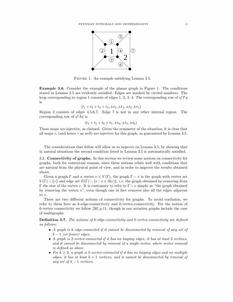
Figure 1. An example satisfying Lemma 3.5.
Example 3.6. Consider the example of the planar graph in Figure 1. The conditionsstated in Lemma 3.5 are evidently satisfied. Edges are marked by circled numbers. Theloop corresponding to region 1 consists of edges 1, 2, 3, 4. The corresponding row of ηtTηis
(t1 + t2 + t3 + t4,±t4,±t3,±t2,±t1) .
Region 2 consists of edges 4,5,6,7. Edge 7 is not in any other internal region. Thecorresponding row of η†Λη is
(t4 + t5 + t6 + t7,±t4,±t5,±t6) .
These maps are injective, as claimed. Given the symmetry of the situation, it is clear thatall maps τi (and hence τ as well) are injective for this graph, as guaranteed by Lemma 3.5.
The considerations that follow will allow us to improve on Lemma 3.5, by showing thatin natural situations the second condition listed in Lemma 3.5 is automatically satisfied.
3.2. Connectivity of graphs. In this section we review some notions on connectivity forgraphs, both for contextual reasons, since these notions relate well with conditions thatare natural from the physical point of view, and in order to improve the results obtainedabove.
Given a graph Γ and a vertex v ∈ V (Γ), the graph Γ r v is the graph with vertex setV (Γ) r {v} and edge set E(Γ) r {e : v ∈ ∂(e)}, i.e. the graph obtained by removing fromΓ the star of the vertex v. It is customary to refer to Γ r v simply as “the graph obtainedby removing the vertex v”, even though one in fact removes also all the edges adjacentto v.
There are two different notions of connectivity for graphs. To avoid confusion, werefer to them here as k-edge-connectivity and k-vertex-connectivity. For the notion ofk-vertex connectivity we follow [26] p.11, though in our notation graphs include the caseof multigraphs.
Definition 3.7. The notions of k-edge-connectivity and k-vertex-connectivity are definedas follows:
• A graph is k-edge-connected if it cannot be disconnected by removal of any set ofk − 1 (or fewer) edges.
• A graph is 2-vertex-connected if it has no looping edges, it has at least 3 vertices,and it cannot be disconnected by removal of a single vertex, where vertex removalis defined as above.
• For k ≥ 3, a graph is k-vertex-connected if it has no looping edges and no multipleedges, it has at least k + 1 vertices, and it cannot be disconnected by removal ofany set of k − 1 vertices.

10 ALUFFI AND MARCOLLI
Figure 2. A splitting of a graph Γ at a vertex v
Thus, 1-vertex-connected and 1-edge-connected simply mean connected, while 2-edge-connected is the one-particle-irreducible (1PI) condition recalled in Definition 1.1. To seehow the condition of 2-vertex-connectivity relates to the physical 1PI condition, we firstrecall the notion of splitting of a vertex in a graph Γ (cf. [26], §4.2).
Definition 3.8. A graph Γ′ is a splitting of Γ at a vertex v ∈ V (Γ) if it is obtained bypartitioning the set E ⊂ E(Γ) of edges adjacent to v into two disjoint non-empty subsets,E = E1 ∪ E2 and inserting a new edge e to whose end vertices v1 and v2 the edges in thetwo sets E1 and E2 are respectively attached (see Figure 2).
We have the following relation between 2-vertex-connectivity and 2-edge-connectivity(1PI). The first observation will be needed in the proof of Proposition 3.13; the second isoffered mostly for contextual reasons.
Lemma 3.9. Let Γ be a graph with at least 3 vertices and no looping edges.
(1) If Γ is 2-vertex-connected then it is also 2-edge-connected (1PI).(2) Γ is 2-vertex-connected if and only if all the graphs Γ′ obtained as splittings of Γ
at any v ∈ V (Γ) are 2-edge-connected (1PI).
Proof. (1): We have to show that, for a graph Γ with at least 3 vertices and no loopingedges, 2-vertex-connectivity implies 2-edge-connectivity. Assume that Γ is not 1PI. Thenthere exists an edge e such that Γ r e has two connected components Γ1 and Γ2. SinceΓ has no looping edges, e has two distinct endpoints v1 and v2, which belong to the twodifferent components after the edge removal. Since Γ has at least 3 vertices, at leastone of the two components contains at least two vertices. Assume then that there existsv 6= v1 ∈ V (Γ1). Then, after the removal of the vertex v1 from Γ, the vertices v and v2
belong to different connected components, so that Γ is not 2-vertex-connected.(2): We need to show that 2-vertex-connectivity is equivalent to all splittings Γ′ being
1PI. Suppose first that Γ is not 2-vertex-connected. Since Γ has at least 3 vertices andno looping edges, the failure of 2-vertex-connectivity means that there exists a vertex vwhose removal disconnects the graph. Let V ⊂ V (Γ) be the set of vertices other than vthat are endpoints of the edges adjacent to v. This set is a union V = V1 ∪ V2 where thevertices in the two subsets Vi are contained in at least two different connected componentsof Γ r v. Then the splitting Γ′ of Γ at v obtained by inserting an edge e such that theendpoints v1 and v2 are connected by edges, respectively, to the vertices in V1 and V2 isnot 1PI.
Conversely, assume that there exists a splitting Γ′ of Γ at a vertex v that is not 1PI.There exists an edge e of Γ′ whose removal disconnects the graph. If e already belongedto Γ, then Γ would not be 1PI (and hence not 2-vertex connected, by (1)), as removal ofe would disconnect it. So e must be the edge added in the splitting of Γ at the vertex v.
Let v1 and v2 be the endpoints of e. None of the other edges adjacent to v1 or v2 is alooping edge, by hypothesis; therefore there exist at least another vertex v′1 6= v2 adjacentto v1, and a vertex v′2 6= v1 adjacent to v2. Since Γ′ r e is disconnected, v′1 and v′2 are
FEYNMAN INTEGRALS AND DETERMINANTS 11
in distinct connected components of Γ′ r e. Since v′1 and v′2 are in Γ r v, and Γ r v iscontained in Γ′ r e, it follows that removing v from Γ would also disconnect the graph.Thus Γ is not 2-vertex-connected. �
The first statement in Lemma 3.9 admits the following analog for 3-connectivity.
Lemma 3.10. Let Γ be a graph with at least 4 vertices, with no looping edges and nomultiple edges. Then 3-vertex-connectivity implies 3-edge-connectivity.
Proof. We argue by contradiction. Assume that Γ is 3-vertex-connected but not 2PI. Weknow it is 1PI because of the previous lemma. Thus, there exist two edges e1 and e2 suchthat the removal of both edges is needed to disconnect the graph. Since we are assumingthat Γ has no multiple or looping edges, the two edges have at most one end in common.
Suppose first that they have a common endpoint v. Let v1 and v2 denote the remainingtwo endpoints, vi ∈ ∂ei, v1 6= v2. If the vertices v1 and v2 belong to different connectedcomponents after removing e1 and e2, then the removal of the vertex v disconnects thegraph, so that Γ is not 3-vertex-connected (in fact not even 2-vertex-connected). If v1
and v2 belong to the same connected component, then v must be in a different component.Since the graph has at least 4 vertices and no multiple or looping edges, there exists at leastanother edge attached to either v1, v2, or v, with the other endpoint w /∈ {v, v1, v2}. If w isadjacent to v, then removing v and v1 leaves v2 and w in different connected components.Similarly, if w is adjacent to (say) v1, then the removal of the two vertices v1 and v2 leavev and w in two different connected components. Hence Γ is not 3-vertex-connected.
Next, suppose that e1 and e2 have no endpoint in common. Let v1 and w1 be theendpoints of e1 and v2 and w2 be the endpoints of e2. At least one pair {vi, wi} belongsto two separate components after the removal of the two edges, though not all four pointscan belong to different connected components, else the graph would not be 1PI. Supposethen that v1 and w1 are in different components. It also cannot happen that v2 and w2
belong to the same component, else the removal of e1 alone would disconnect the graph.We can assume then that, say, v2 belongs to the same component as v1 while w2 belongsto a different component (which may or may not be the same as that of w1). Then theremoval of v1 and w2 leaves v2 and w1 in two different components so that the graph isnot 3-vertex-connected. �
Remark 3.11. While the 2-edge-connected hypothesis on Feynman graphs is very natu-ral from the physical point of view, since it is just the 1PI condition that arises when oneconsiders the perturbative expansion of the effective action of the quantum field theory(cf. [22]), conditions of 3-connectivity (3-vertex-connected or 3-edge-connected) arise in amore subtle manner in the theory of Feynman integrals, in the analysis of Laundau sin-gularities (see for instance [29]). In particular, the 2PI effective action is often consideredin quantum field theory in relation to non-equilibrium phenomena, see e.g. [28], §10.5.1.
3.3. Connectivity and embeddings. We now recall another property of graphs onsurfaces, namely the face width of an embedding ι : Γ → S. The face width fw(Γ, ι) is thelargest number k ∈ N such that every non-contractible simple closed curve in S intersectsΓ at least k times. When S is a sphere, hence ι : Γ → S is a planar embedding, one setsfw(Γ, ι) = ∞.
Remark 3.12. For a graph Γ with at least 3 vertices and with no looping edges, thecondition that an embedding ι : Γ → S is a closed 2-cell embedding is equivalent to theproperties that Γ is 2-vertex-connected and that the embedding has face width fw(Γ, ι) ≥2, see Proposition 5.5.11 of [26].
In particular, this implies that a planar graph with at least three vertices and no loopingedges admits a closed 2-cell embedding in the sphere if and only if it is 2-vertex-connected.
12 ALUFFI AND MARCOLLI
Figure 3. Vertex conditions and 2-cell embeddings.
γ
Figure 4. An edge not in the boundary of two faces.
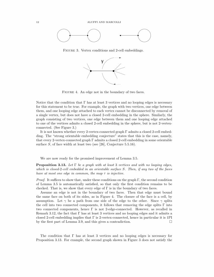
Notice that the condition that Γ has at least 3 vertices and no looping edges is necessaryfor this statement to be true. For example, the graph with two vertices, one edge betweenthem, and one looping edge attached to each vertex cannot be disconnected by removal ofa single vertex, but does not have a closed 2-cell embedding in the sphere. Similarly, thegraph consisting of two vertices, one edge between them and one looping edge attachedto one of the vertices admits a closed 2-cell embedding in the sphere, but is not 2-vertex-connected. (See Figure 3.)
It is not known whether every 2-vertex-connected graph Γ admits a closed 2-cell embed-ding. The “strong orientable embedding conjecture” states that this is the case, namely,that every 2-vertex-connected graph Γ admits a closed 2-cell embedding in some orientablesurface S, of face width at least two (see [26], Conjecture 5.5.16).
We are now ready for the promised improvement of Lemma 3.5.
Proposition 3.13. Let Γ be a graph with at least 3 vertices and with no looping edges,which is closed-2-cell embedded in an orientable surface S. Then, if any two of the faceshave at most one edge in common, the map τ is injective.
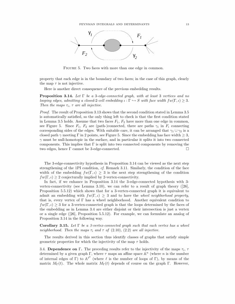
Proof. It suffices to show that, under these conditions on the graph Γ, the second conditionof Lemma 3.5 is automatically satisfied, so that only the first condition remains to bechecked. That is, we show that every edge of Γ is in the boundary of two faces.
Assume an edge is not in the boundary of two faces. Then that edge must boundthe same face on both of its sides, as in Figure 4. The closure of the face is a cell, byassumption. Let γ be a path from one side of the edge to the other. Since γ splitsthe cell into two connected components, it follows that removing the edge splits Γ intotwo connected components, hence Γ is not 2-edge-connected. However, as recalled inRemark 3.12, the fact that Γ has at least 3 vertices and no looping edges and it admits aclosed 2-cell embedding implies that Γ is 2-vertex-connected, hence in particular it is 1PIby the first part of Lemma 3.9, and this gives a contradiction. �
The condition that Γ has at least 3 vertices and no looping edges is necessary forProposition 3.13. For example, the second graph shown in Figure 3 does not satisfy the
FEYNMAN INTEGRALS AND DETERMINANTS 13
γ2
γ1
2
1
F
F
Figure 5. Two faces with more than one edge in common.
property that each edge is in the boundary of two faces; in the case of this graph, clearlythe map τ is not injective.
Here is another direct consequence of the previous embedding results.
Proposition 3.14. Let Γ be a 3-edge-connected graph, with at least 3 vertices and nolooping edges, admitting a closed-2-cell embedding ι : Γ → S with face width fw(Γ, ι) ≥ 3.Then the maps τi, τ are all injective.
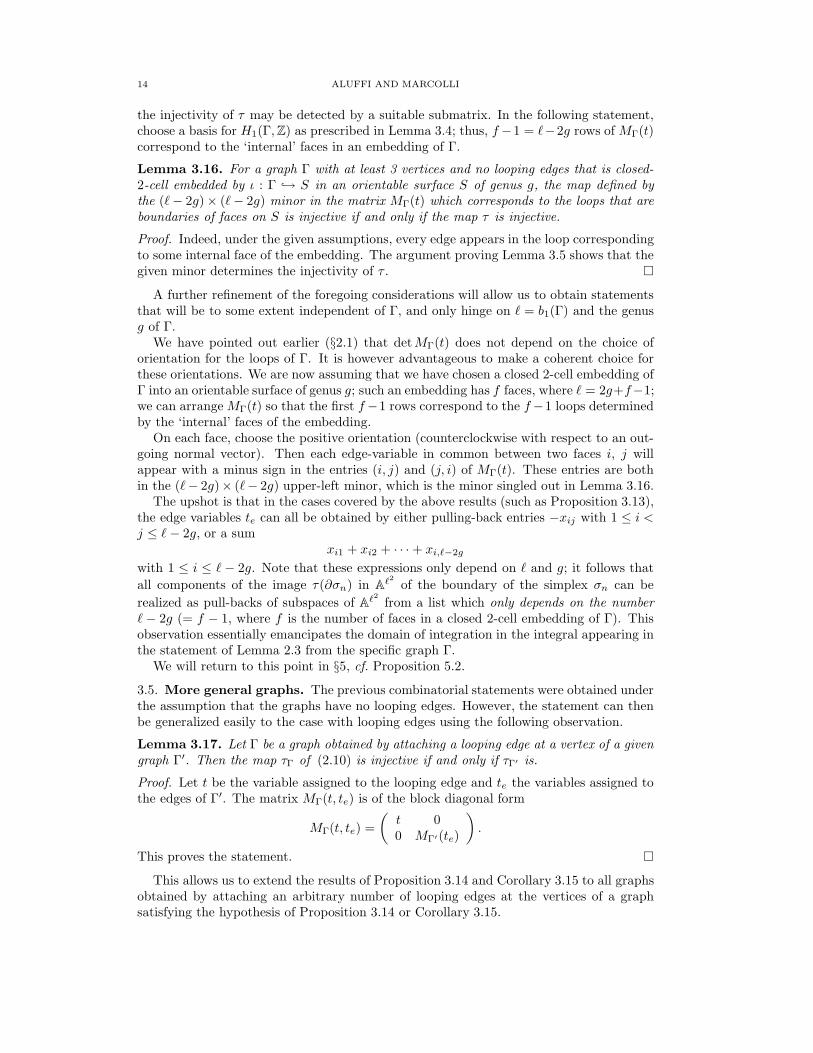
Proof. The result of Proposition 3.13 shows that the second condition stated in Lemma 3.5is automatically satisfied, so the only thing left to check is that the first condition statedin Lemma 3.5 holds. Assume that two faces F1, F2 have more than one edge in common,see Figure 5. Since F1, F2 are (path-)connected, there are paths γi in Fi connectingcorresponding sides of the edges. With suitable care, it can be arranged that γ1 ∪ γ2 is aclosed path γ meeting Γ in 2 points, see Figure 5. Since the embedding has face width ≥ 3,γ must be null-homotopic in the surface, and in particular it splits it into two connectedcomponents. This implies that Γ is split into two connected components by removing thetwo edges, hence Γ cannot be 3-edge-connected. �
The 3-edge-connectivity hypothesis in Proposition 3.14 can be viewed as the next stepstrengthening of the 1PI condition, cf. Remark 3.11. Similarly, the condition of the facewidth of the embedding fw(Γ, ι) ≥ 3 is the next step strengthening of the conditionfw(Γ, ι) ≥ 2 conjecturally implied by 2-vertex-connectivity.
In fact, if we enhance in Proposition 3.14 the 3-edge-connected hypothesis with 3-vertex-connectivity (see Lemma 3.10), we can refer to a result of graph theory ([26],Proposition 5.5.12) which shows that for a 3-vertex-connected graph it is equivalent toadmit an embedding with fw(Γ, ι) ≥ 3 and to have the wheel neighborhood property,that is, every vertex of Γ has a wheel neighborhood. Another equivalent condition tofw(Γ, ι) ≥ 3 for a 3-vertex-connected graph is that the loops determined by the faces ofthe embedding as in Lemma 3.4 are either disjoint or their intersection is just a vertexor a single edge ([26], Proposition 5.5.12). For example, we can formulate an analog ofProposition 3.14 in the following way.
Corollary 3.15. Let Γ be a 3-vertex-connected graph such that each vertex has a wheelneighborhood. Then the maps τi and τ of (2.10), (2.2) are all injective.
The results derived in this section thus identify classes of graphs that satisfy simplegeometric properties for which the injectivity of the map τ holds.
3.4. Dependence on Γ. The preceding results refer to the injectivity of the maps τi, τdetermined by a given graph Γ, where τ maps an affine space An (where n is the number
of internal edges of Γ) to Aℓ2 (where ℓ is the number of loops of Γ), by means of thematrix MΓ(t). The whole matrix MΓ(t) depends of course on the graph Γ. However,
14 ALUFFI AND MARCOLLI
the injectivity of τ may be detected by a suitable submatrix. In the following statement,choose a basis for H1(Γ, Z) as prescribed in Lemma 3.4; thus, f −1 = ℓ−2g rows of MΓ(t)correspond to the ‘internal’ faces in an embedding of Γ.
Lemma 3.16. For a graph Γ with at least 3 vertices and no looping edges that is closed-2-cell embedded by ι : Γ → S in an orientable surface S of genus g, the map defined bythe (ℓ − 2g)× (ℓ − 2g) minor in the matrix MΓ(t) which corresponds to the loops that areboundaries of faces on S is injective if and only if the map τ is injective.
Proof. Indeed, under the given assumptions, every edge appears in the loop correspondingto some internal face of the embedding. The argument proving Lemma 3.5 shows that thegiven minor determines the injectivity of τ . �
A further refinement of the foregoing considerations will allow us to obtain statementsthat will be to some extent independent of Γ, and only hinge on ℓ = b1(Γ) and the genusg of Γ.
We have pointed out earlier (§2.1) that detMΓ(t) does not depend on the choice oforientation for the loops of Γ. It is however advantageous to make a coherent choice forthese orientations. We are now assuming that we have chosen a closed 2-cell embedding ofΓ into an orientable surface of genus g; such an embedding has f faces, where ℓ = 2g+f−1;we can arrange MΓ(t) so that the first f −1 rows correspond to the f −1 loops determinedby the ‘internal’ faces of the embedding.
On each face, choose the positive orientation (counterclockwise with respect to an out-going normal vector). Then each edge-variable in common between two faces i, j willappear with a minus sign in the entries (i, j) and (j, i) of MΓ(t). These entries are bothin the (ℓ− 2g)× (ℓ− 2g) upper-left minor, which is the minor singled out in Lemma 3.16.
The upshot is that in the cases covered by the above results (such as Proposition 3.13),the edge variables te can all be obtained by either pulling-back entries −xij with 1 ≤ i <j ≤ ℓ − 2g, or a sum
xi1 + xi2 + · · · + xi,ℓ−2g
with 1 ≤ i ≤ ℓ − 2g. Note that these expressions only depend on ℓ and g; it follows that
all components of the image τ(∂σn) in Aℓ2 of the boundary of the simplex σn can be
realized as pull-backs of subspaces of Aℓ2 from a list which only depends on the numberℓ − 2g (= f − 1, where f is the number of faces in a closed 2-cell embedding of Γ). Thisobservation essentially emancipates the domain of integration in the integral appearing inthe statement of Lemma 2.3 from the specific graph Γ.
We will return to this point in §5, cf. Proposition 5.2.
3.5. More general graphs. The previous combinatorial statements were obtained underthe assumption that the graphs have no looping edges. However, the statement can thenbe generalized easily to the case with looping edges using the following observation.
Lemma 3.17. Let Γ be a graph obtained by attaching a looping edge at a vertex of a givengraph Γ′. Then the map τΓ of (2.10) is injective if and only if τΓ′ is.
Proof. Let t be the variable assigned to the looping edge and te the variables assigned tothe edges of Γ′. The matrix MΓ(t, te) is of the block diagonal form
MΓ(t, te) =
(
t 00 MΓ′(te)
)
.
This proves the statement. �
This allows us to extend the results of Proposition 3.14 and Corollary 3.15 to all graphsobtained by attaching an arbitrary number of looping edges at the vertices of a graphsatisfying the hypothesis of Proposition 3.14 or Corollary 3.15.

FEYNMAN INTEGRALS AND DETERMINANTS 15
Corollary 3.18. Let Γ be a graph such that, after removing all the looping edges, theremaining graph is 3-vertex-connected with a wheel neighborhood at each vertex. Then themaps τi, τ are all injective.
We can further extend the class of graphs to which the results of this section applyby including those graphs that are obtained from graphs satisfying the hypotheses ofProposition 3.13, Proposition 3.14, Corollary 3.15, or Corollary 3.18 by subdividing edges.
Let en be the edge of Γ that is subdivided in two edges e′n and e′′n to form the graph Γ′.The effect on the graph polynomial is
ΨΓ′(t1, . . . , tn−1, t′n, t′′n) = ΨΓ(t1, . . . , tn−1, t
′n + t′′n),
since the spanning trees of Γ′ are obtained by adding either e′n or e′′n to those spanningtrees of Γ that do not contain en and by replacing en with e′n ∪ e′′n in the spanning treesof Γ that contain en. Thus, notice that in this case the injectivity of the map τ is notpreserved by the operation of splitting edges. However, one can check directly that thisoperation does not affect the nature of the period computed by the Feynman integral, asthe following result shows, so that any result that will show that the Feynman integralis a period of a mixed Tate motive for a class of graphs with no valence two vertices willautomatically extend to graphs obtained by splitting edges.
Proposition 3.19. Let Γ′ be a graph obtained from a given graph Γ by subdividing oneof the edges by inserting a valence two vertex. Then the parametric Feynman integral forΓ′ will be of the form
(3.1)
∫
σn
PΓ(t, p)−(n+1)+Dℓ/2tnωn
ΨΓ(t)−(n+1)+(ℓ+1)D/2,
with n = #Eint(Γ).
Proof. When one subdivides an edge as above, the Feynman rules imply that one finds ascorresponding Feynman integral an expression of the form
∫
δ(∑
i ǫv,iki +∑
j ǫv,jpj)
q1 · · · qn−1q2n
dDk1
(2π)D· · ·
dDkn
(2π)D,
where the qi(ki) = k2i + m2 are the quadratic forms that give the propagators associated
to the internal edges of the graph. We have used the constraint δ(kn − kn+1) for the twomomentum variables associated to the two parts of the split edge, so that we find q2
n inthe denominator. One then uses the usual formula
1
qa1
1 · · · qan
n=
Γ(a1 + · · · + an)
Γ(a1) · · ·Γ(an)
∫
Rn
+
ta1−11 · · · tan−1
n δ(1 −∑
i ti)
(t1q1 + · · · tnqn)a1+···+an
to obtain the parametric form of the Feynman integral. In our case this gives
1
q1 · · · qn−1q2n
= n!
∫
σn
tn dt1 · · · dtn(t1q1 + · · · tnqn)n+1
.
Thus, one obtains the parametric form of the Feynman integral as∫
dDx1 · · · dDxℓ
(∑
i tiqi)n+1= Cℓ,n+1 det(MΓ(t))−D/2VΓ(t, p)−(n+1)+Dℓ/2,
where VΓ(t, p) = PΓ(t, p)/ΨΓ(t) and with
Cℓ,n+1 =
∫
dDx1 · · · dDxℓ
(1 +∑
k x2k)n+1
.
This gives (3.1). �
16 ALUFFI AND MARCOLLI
In particular Proposition 3.19 shows that the parametric Feynman integral for thegraph Γ′ is still a period of the same type as that of the graph Γ, since it is still a periodassociated to the complement of the graph hypersurface XΓ and evaluated over the same
simplex σn. Only the algebraic differential form changes from Ψ−D/2Γ VΓ(t, p)−n+Dℓ/2ωn to
Ψ−D/2Γ VΓ(t, p)−(n+1)+Dℓ/2tnωn, but this does not affect the nature of the period, at least
in the “stable range” where D is sufficiently large (Dℓ/2 > n).
4. The motive of the determinant hypersurface complement
Our work in §2 and §3 relates the complexity of a Feynman integral over a graphsatisfying suitable combinatorial conditions to the complexity of the motive
m(Aℓ2 r Dℓ, ΣΓ r (ΣΓ ∩ Dℓ))
whose realizations give the relative cohomology of the pair of the complement of thedeterminant hypersurface and a normal crossings divisor ΣΓ containing the image of theboundary τΓ(∂σn), as in Lemma 5.1 below (see Corollary 2.4, Proposition 3.13 and ff.).
In this section we exhibit an explicit filtration of the complement of the determinant
hypersurface, from which we can directly prove that the motive of Aℓ2 r DΓ is mixed Tate.
We use this filtration to compute explicitly the class of Aℓ2 r DΓ in the Grothendieck
group of varieties, as well as the class of the projective version Pℓ2−1 r Dℓ.Notice that the mixed Tate nature of the motive of the determinant hypersurface also
follows directly from the results of Belkale–Brosnan [3], or from those of Biglari [5], [6], butwe prefer to give here a very explicit computation, which will be useful as a preliminaryfor the similar but more involved analysis of the loci that contain the boundary of thedomain of integration that we discuss in the following sections.
4.1. The motive. As we already argued, it is more natural to consider the graph hyper-surfaces XΓ in the affine space An, instead of the projective XΓ in Pn−1. Thus, here also
we work with the affine space Aℓ2 parametrizing ℓ × ℓ matrices. The cone Dℓ over thedeterminant hypersurface consists of matrices of rank < ℓ. Realizing the complement of
Dℓ in Aℓ2 amounts then to ‘parametrizing’ matrices M of rank exactly ℓ.It is clear how this should be done:
— The first row of M must be a nonzero vector v1;— The second row of M must be a vector v2 that is nonzero modulo v1;— The third row of M must be a vector v3 that is nonzero modulo v1 and v2;— And so on.
To formalize this construction, let E be a fixed ℓ-dimensional vector space, and workinductively. The first steps of the construction are as follows.
— Denote by W1 the variety E r {0};— Note that W1 is equipped with a trivial vector bundle E1 = E ×W1, and with a
line bundle S1 := L1 ⊆ E1 whose fiber over v1 ∈ W1 consists of the line spannedby v1;
— Let W2 ⊆ E1 be the complement E1 r L1;— Note that W2 is equipped with a trivial vector bundle E2 = E ×W2, and two line
subbundles of E2: the pull-back of L1 (still denoted L1) and the line-bundle L2
whose fiber over v2 ∈ W2 consists of the line spanned by v2;— By construction, L1 and L2 span a rank-2 subbundle S2 of E2;— Let W3 ⊆ E2 be the complement E2 r S2;— And so on.
FEYNMAN INTEGRALS AND DETERMINANTS 17
Inductively: at the k-th step, this procedure produces a variety Wk, endowed withk line bundles L1, . . . , Lk spanning a rank-k subbundle Sk of the trivial vector bundleEk := E ×Wk. If Sk ( Ek, define Wk+1 := Ek r Sk. Let Ek+1 = E ×Wk+1, and defineline subbundles L1, . . . , Lk to be the pull-backs of the like-named line bundles on Wk; andlet Lk+1 be the line bundle whose fiber over vk+1 is the line spanned by vk+1. The linebundles L1, . . . , Lk+1 span a rank-k+1 subbundle Sk+1 of Ek+1, and the construction cancontinue. The sequence stops at the ℓ-th step, where Sℓ has rank ℓ, equal to the rank ofEℓ, so that Eℓ r Sℓ = ∅.
Lemma 4.1. The variety Wℓ constructed as above is isomorphic to Aℓ2 r Dℓ.
Proof. Each variety Wk maps to Aℓ2 as follows: a point of Wk determines k vectorsv1, . . . , vk, and can be mapped to the matrix whose first k rows are v1, . . . , vk resp. (andthe remaining rows are 0). By construction, this matrix has rank exactly k. Conversely,any such rank k matrix is the image of a point of Wk, by construction. �
In particular, we have the following result on the bundles Sk involved in the constructiondescribed above.
Lemma 4.2. The bundle Sk over the variety Wk is trivial for all 1 ≤ k ≤ ℓ.
Proof. Points of Wk are parameterized by k-tuples of vectors v1, . . . , vk spanning Sk ⊆Kℓ ×Wk = Ek. This means precisely that the map
Kk ×Wkα→ Sk
defined byα : ((c1, . . . , cr), (v1, . . . , vr)) 7→ c1v1 + · · · + crvr
is an isomorphism. �
Recall that, given a triangulated category D, a full subcategory D′ is a triangulatedsubcategory if and only if it is invariant under the shift T of D and for any distinguishedtriangle
A → B → C → A[1]
for D where A and B are in D′ there is an isomorphism C ≃ C′ with C′ also in D′. A fulltriangulated subcategory D′ ⊂ D is thick if it is closed under direct sums.
Let MDK be the Voevodsky triangulated category of mixed motives over a field K,[33]. The triangulated category DMTK of mixed Tate motives is the full triangulatedthick subcategory of MDK generated by the Tate objects Q(n). It is known that, over anumber field K, there is a canonical t-structute on DMTK and one can therefore constructan abelian category MTK of mixed Tate motives (see [24]).
We then have the following result on the nature of the motive of the determinanthypersurface complement.
Theorem 4.3. The determinant hypersurface complement Aℓ2 r Dℓ defines an object inthe category DMTK of mixed Tate motives.
Proof. First recall that by Proposition 4.1.4 of [33], over a field K of characteristic zero aclosed embedding Y ⊂ X determines a distinguished triangle
m(Y ) → m(X) → m(X r Y ) → m(Y )[1]
in MDK. Here we use the notation m(X) for the motivic complex with compact supportdenoted by Cc
∗(X) in [33]. In particular, if m(Y ) and m(X) are in DMTK then m(X r Y )is isomorphic to an object in DMTK, by the property of full triangulated subcategoriesrecalled above. Similarly, using the invariance of DMTK under the shift, if m(Y ) andm(X r Y ) are in DMTK then m(X) is isomorphic to an object in DMTK.
18 ALUFFI AND MARCOLLI
We also know (see §1.2.3 of [8]) that in the Voevodsky category MDK one invertsthe morphism X × A1 → X induced by the projection, so that taking the product withan affine space Ak is an isomorphism at the level of the corresponding motives and forthe motivic complexes with compact support this gives m(X × A1) = m(X)(−1)[2], seeCorollary 4.1.8 of [33]. Thus, for any given m(X) in DMTK, the motive m(X × Ak) isobtained from m(X) by Tate twists and shifts, hence it is also in DMTK.
These two properties of the derived category DMTK of mixed Tate motives suffice to
show that the motive of the affine hypersurface complement Aℓ2 r Dℓ is mixed Tate,
(4.1) m(Aℓ2 r Dℓ) ∈ Obj(DMTQ).
In fact, one sees from the inductive construction of Aℓ2 r Dℓ described above that at eachstep we are dealing with varieties defines over K = Q and we now show that, at each step,the corresponding motives are mixed Tate.
Single points obviously belong to the category of mixed Tate motives. At the first step,one takes the complement W1 of a point in an affine space, which gives a mixed Tate motiveby the first observation above on distinguished triangles associated to closed embeddings.At the next step one considers the complement of the line bundle S1 inside the trivialvector bundle E1 over W1. Again, both m(S1) and m(E1) are mixed Tate motives, sinceboth are products by affine spaces by Lemma 4.2 above, hence m(E1 r S1) is also mixedTate. The same argument shows that, for all 1 ≤ k ≤ ℓ, the motive m(Ek r Sk) is mixedTate, by repeatedly using Lemma 4.2 and the two properties of DMTQ recalled above. �
4.2. The class in the Grothendieck ring. Lemma 4.1 suffices to obtain an explicitformula for the class in the Grothendieck ring of varieties of the complement of the deter-minant hypersurface. This is of course well-known: see for example [3], §3.3.
Proposition 4.4. In the affine case the class in the Grothendieck ring of varieties is
(4.2) [Aℓ2 r Dℓ] = L(ℓ
2)ℓ
∏
i=1
(Li − 1)
where L is the class of A1. In the projective case, the class is
(4.3) [Pℓ2−1 r Dℓ] = L(ℓ
2)ℓ
∏
i=2
(Li − 1).
Proof. Using Lemma 4.1 one sees inductively that the class of Wk is given by
(4.4)[Wk] = (Lℓ − 1)(Lℓ − L)(Lℓ − L2) · · · (Lℓ − Lk−1)
= L(k
2)(Lℓ − 1)(Lℓ−1 − 1) · · · (Lℓ−k+1 − 1).
This completes the proof. �
The class (4.3) can be written equivalently in the form
(4.5) [Pℓ2−1 r Dℓ] = (L[P1]T) · (L2[P2]T) · (L3[P3]T) · · · (Lℓ−1[Pℓ−1]T),
where L = [A1] and T = [Gm] is the class of the multiplicative group. Here the motiveLℓ[P1] · · · [Pℓ−1] can be thought of as the motive of the “variety of frames”.
Example 4.5. In the cases ℓ = 2 and ℓ = 3, the class of Pℓ2−1 rDℓ is given, respectively,by
L3 − L and L8 − L5 − L6 + L3.

FEYNMAN INTEGRALS AND DETERMINANTS 19
(Note however that, for ℓ ≥ 5, coefficients other than 0, ±1 appear in the class.) Thus,the class [Dℓ] is given, for ℓ = 2 and ℓ = 3 by the expressions
[D2] = L2 + 2L + 1 = (L + 1)2
[D3] = L7 + 2L6 + 2L5 + L4 + L2 + L + 1 = (L3 − L + 1)(L2 + L + 1)2.
The ℓ = 2 case is otherwise evident: D2 is the set of rank-1, 2 × 2–matrices, and as suchit may be realized as P1 × P1, with the indicated class. The ℓ = 3 case can also be easilyverified independently.
5. Relative cohomology and mixed Tate motives
We now assume that Γ is a graph satisfying the condition studied in §2 and §3: the map τis injective. By Proposition 3.13, this is the case if Γ has at least 3 vertices, no loopingedges, and is closed-2-cell embedded in an orientable surface in such a way that any two ofthe faces determined by the embedding have at most one edge in common. Proposition 3.14and Corollary 3.15 provide us with specific combinatorial conditions ensuring that this isthe case. For instance, all 3-edge connected planar graphs are included in this class.
Also note that by the considerations in §3.5 (especially Lemma 3.17 and Proposi-tion 3.19), any estimate for the complexity of Feynman integrals for graphs satisfyingthese conditions generalizes automatically to the larger class of graphs obtained from thoseconsidered here by adding arbitrarily many looping edges, and by arbitrarily subdividingedges.
5.1. Algebraic simplexes and normal crossing divisors. In our setting and underthe injectivity assumption, the property that the Feynman integral (1.9) is a period of amixed Tate motive (modulo divergences) would follow from showing that a certain relativecohomology is a realization of a mixed Tate motive. Instead of the relative cohomology
Hn−1(Pn−1 r XΓ, Σn r (Σn ∩ XΓ))
considered in [10], [9], we consider here a different relative cohomology, where the hypersur-
face complement Pn−1 r XΓ is replaced by the complement Pℓ2−1 rDℓ of the determinant
hypersurface, or better its affine counterpart Aℓ2 rDℓ, and instead of the algebraic simplex
Σn = {t : t1 · · · tn = 0}, we consider a locus ΣΓ in Aℓ2 that pulls back to the algebraicsimplex Σn under the map τ of (2.10) and that consists of a union of n linear subspaces
of codimension one in Aℓ2 that meet the image of An under τ along divisors with normalcrossings. The following observation is a direct consequence of the construction of thematrix MΓ(t) (cf. §2.1).
Lemma 5.1. Suppose given a graph Γ such that the corresponding maps τ and τi areinjective. Then the n coordinates ti associated to the internal edges of Γ can be written as
preimages via the (injective) map τ : An → Aℓ2 of n linear subspaces Xi of codimension 1
in Aℓ2 . These n subspaces form a divisor ΣΓ with normal crossings in Aℓ2 .
Proof. Consider the various possible cases for a specific edge listed in Lemma 2.2. In thethird case listed there, where there are two loops ℓi, ℓj containing e, and not having anyother edge in common, the variable te is immediately expressed as the pullback to An of
a coordinate in Aℓ2 . Consider then the second case listed in Lemma 2.2, where an edge ebelongs to a single loop ℓi. Under the assumption that the map τi is injective, then anylinear combination of the variables corresponding to the edges in the i-th loop may bewritten as a linear combination of coordinates of the i-th row. �
20 ALUFFI AND MARCOLLI
The considerations in §3.4 allow us to improve this observation, by passing to a largernormal crossing divisor, so that one can generate all the ΣΓ from the components of asingle normal crossings divisor Σℓ,g that only depends on the number of loops of the graphand on the minimal genus of the embedding of the graph on a Riemann surface. Weformalize this remark as follows.
Proposition 5.2. There exists a normal crossings divisor Σℓ,g ⊂ Aℓ2 , which is a union
of N =(
f2
)
linear spaces
(5.1) Σℓ,g := X1 ∪ · · · ∪ XN ,
such that, for all graphs Γ with ℓ loops and genus g closed 2-cell embedding, the preimageunder τ = τΓ of the union ΣΓ of a subset of components of Σℓ,g is the algebraic simplex
Σn in An. More explicitly, the divisor Σℓ,g can be described by the N =(
f2
)
equations
(5.2)
{
xij = 0 1 ≤ i < j ≤ f − 1xi1 + · · · + xi,f−1 = 0 1 ≤ i ≤ f − 1,
where f = ℓ − 2g + 1 is the number of faces of the embedding.
Proof. Using Lemma 3.16, we know that the injectivity of an (ℓ − 2g)× (ℓ − 2g) minor ofthe matrix MΓ suffices to control the injectivity of the map τ . We can in fact arrange sothat the minor is the upper-left part of the ℓ× ℓ ambient matrix. Then, as in Lemma 5.1,the hyperplanes in An associated to the coordinates ti can be obtained by pulling backlinear spaces along this minor. On the diagonal of the (f − 1)× (f − 1) submatrix we findall edges making up each face, with a positive sign. It follows that the pull-backs of theequations (5.2) produce a list of all the edge variables, possibly with redundancies. The
components of Σℓ,g that form the divisor ΣΓ are selected by eliminating those components
of Σℓ,g that contain the image of the graph hypersurface (i.e. coming from the zero entriesof the matrix MΓ(t)). �
Thus, for every Γ satisfying the conditions recalled at the beginning of the section(for example, every 3-edge connected planar graph, or every graph obtained from one ofthese by adding looping edges or subdividing edges), the nature of period appearing as aFeynman integral over Γ in the sense explained in §2 is controlled by the motive
(5.3) m(Aℓ2 r Dℓ, ΣΓ r (Dℓ ∩ ΣΓ)),
for a normal crossing divisor ΣΓ ⊂ Aℓ2 consisting of a subset of components of the fixed
(for given ℓ and g) normal crossing divisor Σℓ,g ⊂ Aℓ2 introduced above.More explicitly, the boundary of the topological simplex σn, that is, the domain of
integration of the Feynman integral in Lemma 2.3, satisfies
(5.4) τ(∂σn) ⊂ ΣΓ ⊂ Σℓ,g.
Thus, the main goal here will be to understand the motivic nature of the complement
(5.5) ΣΓ r (Dℓ ∩ ΣΓ).
Since ΣΓ consists of components from the fixed normal crossing divisor Σℓ,g, this ques-tion will be recast in terms that only depend on ℓ and g: we show in Corollary 5.4below that, using the inclusion–exclusion principle applied to the components of Σℓ,g, it
is possible to answer these questions simultaneously for all the divisors ΣΓ, for all graphswith ℓ loops and genus g, by investigating the nature of a motive constructed out of theintersections of the components of the divisor Σℓ,g.
Notice in fact that one can derive the case of Σℓ,g from the case of g = 0, since
Σℓ,g ⊆ Σℓ,0, corresponding to an (ℓ − 2g) × (ℓ − 2g) minor of the matrix MΓ(t).
FEYNMAN INTEGRALS AND DETERMINANTS 21
There are general and explicit conditions (see [18], Proposition 3.6) implying that therelative cohomology of a pair (X, Y ) comes from a mixed Tate motive m(X, Y ) (see also[19] for a concrete application to the geometric case of moduli spaces of curves). In general,these rely on assumptions on the divisors involved and their associated stratification, whichmay not directly apply to the cases considered here. We discuss here a direct approach toconstructing stratifications of our loci Σℓ,g r (Dℓ ∩ Σℓ,g) that can be used to investigatethe nature of the motive (5.3).
5.2. Inclusion–exclusion. The procedure we follow will be the one outlined above, basedon the divisors Σℓ,g and the inclusion–exclusion principle. Since we already know by the
results of §4 that the complement X = Aℓ2rDℓ is a mixed Tate motive, we aim at providinga direct argument showing that Y = ΣΓr(ΣΓ∩Dℓ) also is a mixed Tate motive. The sameargument used in §4 based on the distinguished triangles in the Voevodsky triangulatedcategory of mixed Tate motives [33] would then show that the relative cohomology of thepair (X, Y ) comes from an object m(X, Y ) ∈ Obj(DMTQ).
As a first step we transform the problem of a complement in a union of linear spacesinto an equivalent formulation in terms of intersections of linear spaces, using inclusion–exclusion. For a collection {Zi}i∈I of varieties Zi we set
(5.6) Z◦I := (∩i∈IZi) r (∪j 6∈IZj).
Notice that, for all I,∩i∈IZi = ∐J⊇IZ
◦J .
This is a disjoint union. We then have the following result.
Lemma 5.3. Let Z1, . . . , Zm be varieties; assume that the intersections ∩i∈IZi are mixedTate, for all nonempty I ⊆ {1, . . . , m}. Then Z1 ∪ · · · ∪ Zm is mixed Tate.
Proof. We want to show that Z◦I is mixed Tate for all nonempty I ⊆ {1, . . . , m}. To see
this, notice that it is true by hypothesis for I = {1, . . . , m}, since in this case Z◦I = ∩i∈IZi.
Thus, it suffices to prove that if it is true for all I with |I| > k, then it is true for all I with|I| = k (provided k ≥ 1). Recall that, as we already used in §4 above, the distinguishedtriangles in the Voevodsky category of mixed Tate motives imply that, if X → Y is aclosed embedding, and U = Y r X the complement, then if any two of X, Y, U are mixedTate so is the third as well. The result then follows from the combined use of this property,the hypothesis, and the identity
Z◦I = (∩i∈IZi) r (∐J)IZ
◦J) .
Since we haveZ1 ∪ · · · ∪ Zm = ∐I 6=∅Z
◦I ,
we conclude that the union Z1 ∪ · · · ∪ Zm is mixed Tate, again by the property of mixedTate motives mentioned above. �
Now, we have observed that for every graph Γ with ℓ loops and genus g (and satisfying
the condition specified at the beginning of the section) the divisor ΣΓ consists of compo-
nents of the divisor Σℓ,g. Therefore, the strata of ΣΓ are unions of strata from Σℓ,g. Wecan then reformulate our main problem as follows.
Corollary 5.4. Let, as above, Σℓ,g = X1∪· · ·∪XN and let ΣΓ be the divisors constructed
out of subsets of components of Σℓ,g, associated to the individual graphs. Then, for all
graphs Γ with ℓ loops and genus g, the complement ΣΓ r (Dℓ ∩ ΣΓ) is mixed Tate if thelocus
(5.7) (∩i∈IXi) r Dℓ
is mixed Tate for all I ⊆ {1, . . . , N}, I 6= ∅.
22 ALUFFI AND MARCOLLI
Proof. This is a direct consequence of Lemma 5.3. �
Corollary 5.4 encapsulates the main reformulation of our problem, mentioned at theend of §1: the target becomes that of proving that the loci (∩i∈IXi) r Dℓ determined
by the normal crossing divisor Σℓ,g are mixed Tate. This result shows that, although in
principle one is working with a different divisor ΣΓ for each graph Γ, in fact it suffices to
consider the divisor Σℓ,g, for fixed number of loops ℓ and genus g. It is conceivable that
the loci associated to a specific graph (that is, to a specific choice of components of Σℓ,g)
may be mixed Tate while the loci corresponding to the whole divisor Σℓ,g is not. As we areseeking an explanation that would imply that all periods arising from Feynman integralsare periods of mixed Tate motives, we will optimistically venture that all loci (∩i∈IXi)rDℓ
may in fact turn out to be mixed Tate, for all ℓ and for g = 0: by Corollary 5.4, it wouldfollow that all complements ΣΓ r (Dℓ ∩ ΣΓ) are mixed Tate, for all graphs Γ (satisfyingour running combinatorial hypothesis).
Our task is now to formulate this working hypothesis as a more concrete problem.
The intersection ∩i∈IXi is a linear subspace of codimension |I| in Aℓ2 ; in general, theintersection of a linear subspace with the determinant is not mixed Tate (for example, the
intersection of a general A3 with D3 is a cone over a genus-1 curve). Thus, we have tounderstand in what sense the intersections ∩i∈IXi appearing in Corollary 5.4 are special;the following lemma determines some key features of these subspaces.
Lemma 5.5. Let E be a fixed ℓ-dimensional vector space, as in §4.1 above. Every I ⊆{1, . . . , N} as above determines a choice of linear subspaces V1, . . . , Vℓ of E, such that
(5.8) ∩k∈IXk = {(v1, . . . , vℓ) ∈ Aℓ2 | ∀i, vi ∈ Vi}.
(Here, we denote an ℓ × ℓ matrix in Aℓ2 by its ℓ row-vectors vi ∈ E.)Further, dimVi ≥ i − 1. Further still, there exists a basis (e1, . . . , eℓ) of E such that
each space Vi is the span of a subset (of cardinality ≥ i − 1) of the vectors ej.
Proof. Recall (Proposition 5.2) that the components Xk of Σℓ,g consist of matrices forwhich either the (i, j) entry xij equals 0, for 1 ≤ i < j ≤ ℓ − 2g, or
xi1 + · · · + xi,ℓ−2g = 0
for 1 ≤ i ≤ ℓ − 2g. Thus, each Xk consists of ℓ-tuples (v1, . . . , vℓ) for which exactly onerow vi belongs to a fixed hyperplane of E, and more precisely to one of the hyperplanes
(5.9) x1 + · · · + xℓ−2g = 0 , x2 = 0 , · · · , xℓ−2g = 0
(with evident notation). The statement follows by choosing Vi to be the intersection ofthe hyperplanes corresponding to the Xk in row i, among those listed in (5.9). Since thereare at most ℓ − 2g − i + 1 hyperplanes Xk in the i-th row,
dim Vi ≥ ℓ − (ℓ − 2g − i + 1) = 2g + i − 1 ≥ i − 1 .
Finally, to obtain the basis (e1, . . . , eℓ) mentioned in the statement, simply choose thebasis dual to the basis (x1 + · · · + xℓ−2g, x2, . . . , xℓ) of the dual space to E. �
5.3. The main questions. In view of Lemma 5.5, for any choice V1, . . . , Vℓ of subspacesof an ℓ-dimensional space E, let
(5.10) F(V1, . . . , Vℓ) := {(v1, . . . , vℓ) ∈ Aℓ2 | ∀k, vk ∈ Vk} r Dℓ
denote the complement of the determinant hypersurface in the set of matrices determinedby V1, . . . , Vℓ. An optimistic version of the question we are led to is:
Question Iℓ. Let V1, . . . , Vℓ be subspaces of an ℓ-dimensional vector space. Is the locusF(V1, . . . , Vℓ) mixed Tate?
FEYNMAN INTEGRALS AND DETERMINANTS 23
By Corollary 5.4 and Lemma 5.5, an affirmative answer to Question Iℓ implies that thecomplement ΣΓ r (Dℓ ∩ ΣΓ) is mixed Tate for all graphs Γ with ℓ loops and satisfying thecombinatorial condition given at the beginning of this section. Modulo divergence issues,this would imply that all Feynman integrals corresponding to these graphs are periods ofmixed Tate motives. We will give an affirmative answer to Question Iℓ for ℓ ≤ 3, in §6.
As Lemma 5.5 is in fact more precise, the same conclusion would be reached by an-swering affirmatively the following weak version of Question Iℓ:
Question IIℓ. Let (e1, . . . , eℓ) be a basis of an ℓ-dimensional vector space. For i =1, . . . , ℓ, let Vi be a subspace spanned by a choice of ≥ i− 1 basis vectors. Is F(V1, . . . , Vℓ)mixed Tate?
Notice that, when Vk = E for all k, both questions reproduce the statement about
the hypersurface complement Aℓ2 r Dℓ proved in §4.1. One might expect that a similarinductive procedure would provide a simple approach to these questions. It is natural toconsider the following apparent refinement of Question Iℓ for 1 ≤ r ≤ ℓ (and we couldsimilarly consider an analogous refinement Question II′ℓ,r of Question IIℓ):
Question I′ℓ,r. In a vector space E of dimension ℓ, and for any choice of subspacesV1, . . . , Vr of E, let
Fℓ(V1, . . . , Vr) = {(v1, . . . , vr) | vi ∈ Vi and dim〈v1, . . . vr〉 = r} .
Is the locus Fℓ(V1, . . . , Vr) mixed Tate?
Question Iℓ is then the same as Question I′ℓ,ℓ; and Question I′ℓ,r is obtained by takingVr+1 = · · · = Vℓ = E in Question Iℓ: thus, answering Question Iℓ is equivalent to answeringQuestion I′ℓ,r for all r ≤ ℓ.
Now, for all ℓ, the case r = 1 is immediate: Fℓ(V1) consists of all nonzero vectorsin V1, which is trivially mixed Tate. One could then hope that an inductive proceduremay yield a method for increasing r. This is carried out in §6 for r = 2 and r = 3 (inparticular, we give an affirmative answer to Question Iℓ for ℓ ≤ 3); but this approachquickly leads to the analysis of several different cases, with an increase in complexity thatmakes further progress along these lines seem unlikely. The main problem is that once alltuples (v1, . . . , vk) of linearly independent vectors such that vi ∈ Vi have been constructed,controlling
dim(Vk+1 ∩ 〈v1, . . . , vk〉)
requires consideration of a range of possibilities that depend on the position of the vectorsvi and their spans vis-a-vis the position of the next space Vk+1. The number of thesepossibilities increases rapidly. A similar approach to the simpler (but sufficient for ourpurposes) Question II does not appear to circumvent this problem.
There are special cases where an inductive argument works nicely. We mention twohere.
• Suppose that all the Vk in (5.10) are hyperplanes in E. Then F(V1, . . . , Vℓ) ismixed Tate.
In this case, following the inductive argument mentioned above, the only possibilitiesfor Vk+1 ∩ 〈v1, . . . , vk〉 are 〈v1, . . . , vk〉, and a hyperplane in 〈v1, . . . , vk〉. The first occurswhen
〈v1, . . . , vk〉 ⊆ Vk.
This locus is under control, since it amounts to doing the whole construction in Vk ratherthan E, i.e. one can argue by induction on the dimension of E. Thus, this locus is mixedTate. The other case gives a locus that is the complement of this mixed Tate variety in
24 ALUFFI AND MARCOLLI
another mixed Tate variety, hence, by the same argument about closed embeddings anddistinguished triangles used in §4, it is also mixed Tate.
• Suppose V1 ⊆ V2 ⊆ · · · ⊆ Vr; then Fℓ(V1, . . . , Vr) is mixed Tate.
Indeed, in this case 〈v1, . . . , vk〉 ⊆ Vk+1 for all k. The condition on vk+1 is simplyvk+1 ∈ Vk+1 r 〈v1, . . . , vk〉, and these conditions clearly produce a mixed Tate locus.Arguing as in §4.1, the class of Fℓ(V1, . . . , Vr) is immediately seen to equal
(Ld1 − 1)(Ld2 − L)(Ld3 − L2) · · · (Ldr − Lr−1)
in this case, where dk = dimVk.
5.4. A reformulation. For given subspaces Vi ⊂ E, the inductive approach suggested byQuestion I′ℓ,r aims at constructing the set of ℓ-uples (v1, . . . , vℓ) with the two properties
(1) vi ∈ Vi;(2) dim〈v1, . . . , vr〉 = r, for all r,
and proving inductively that these loci are mixed Tate, in order to show that the loci(5.10) are mixed Tate. By (2), the sets
0 ⊂ 〈v1〉 ⊂ 〈v1, v2〉 ⊂ · · · ⊂ 〈v1, . . . , vℓ〉 = E
form a complete flag in E; let Er = 〈v1, . . . , vr〉. Our main question can then be phrasedin terms of these moving complete flags:
Question IIIℓ. Let V1, . . . , Vℓ be subspaces of an ℓ-dimensional vector space E, and letdi, ei be integers. Is the locus Flagℓ,{di,ei}({Vi}) of complete flags
0 ⊂ E1 ⊂ E2 ⊂ · · · ⊂ Eℓ = E
such that
• dimEi ∩ Vi = di
• dimEi ∩ Vi+1 = ei
mixed Tate?
An affirmative answer to this question (for all choices of di, ei) would give an affirmativeanswer to our main Question Iℓ. Indeed, the locus F(V1, . . . , Vℓ) is a fibration on the locusFlagℓ,{di,ei}({Vi}) determined in Question IIIℓ. Concretely, the procedure constructing
the tuples (v1, . . . , vℓ) in F(V1, . . . , Vℓ) over a flag E• in this locus is:
• Choose v1 ∈ (E1 ∩ V1) r {0};• Choose v2 ∈ (E2 ∩ V2) r (E1 ∩ V2);• Choose v3 ∈ (E3 ∩ V3) r (E2 ∩ V3);• etc.
The class of F(V1, . . . , Vℓ) in the Grothendieck group would then be computed as a sumof terms
[Flagℓ,{di,ei}({Vi})] · (Ld1 − 1)(Ld2 − Le1 )(Ld3 − Le2 ) · · · (Ldr − Ler−1) .
The set of flags E• satisfying conditions analogous to those specified in Question IIIℓ withrespect to all terms of a fixed flat E′
• (that is: with prescribed dim(Ei ∩ E′j) for all i and
j) is a cell of the corresponding Schubert variety in the flag manifold.It follows that Flagℓ,{di,ei}({Vi}) is a disjoint union of cells, and thus certainly mixed
Tate, if the Vi’s form a complete flag. This gives a high-brow alternative viewpoint for thelast case mentioned in §5.3.
By the same token, the set of flags E• for which dimEi ∩ F is a fixed constant is aunion of Schubert cells in the flag manifold, for all subspaces F . It follows that the locusFlagℓ,{di,ei}({Vi}) of Question IIIℓ is an intersection of unions of Schubert cells in the flag
manifold. Such loci were studied e.g. in [16], [17], [30], [31].
FEYNMAN INTEGRALS AND DETERMINANTS 25
6. Motives and manifolds of frames
The manifolds of r-frames in a given vector space are defined as follows.
Definition 6.1. Let F(V1, . . . , Vr) ⊂ V1 × · · · × Vr denote the locus of r-tuples of linearlyindependent vectors in a vector space, where each vi is constrained to belong to the givensubspace Vi.
These are the loci appearing in Question I′ℓ,r; we now omit the explicit mention of thedimension ℓ of the ambient space. The question we consider here is the one formulatedin §5.3, namely to establish when the motive of the manifold of frames F(V1, . . . , Vr) ismixed Tate. A possible strategy to answering this question is based on the following simpleobservations.
Lemma 6.2. Let V1, . . . , Vr be subspaces of a given vector space V . Let vr ∈ Vr, andlet π : V → V ′ := V/〈vr〉 be the natural projection. Let v1, . . . , vr−1 be vectors suchthat vi ∈ Vi, and π(v1), . . . , π(vr−1) are linearly independent. Then v1, . . . , vr are linearlyindependent.
Proof. The dimension of π(〈v1, . . . , vr−1〉) = 〈π(v1), . . . , π(vr−1)〉 is r − 1 by hypothesis,therefore dimπ−1(π(〈v1, . . . , vr−1〉)) = r. Since π−1(π(〈v1, . . . , vr−1〉)) ⊆ 〈v1, . . . , vr〉, itfollows that dim〈v1, . . . , vr〉 = r, as needed. �
A second equally elementary remark is that for a given v′ 6= 0 in the quotient V/〈vr〉,and letting as above π denote the projection V → V/〈vr〉, π−1(v′) ∩ Vi consists of eithera single vector, if vr 6∈ Vi, or a copy of the field k, if vr ∈ Vi.
This implies the following.
Lemma 6.3. Suppose given a stratification {Sα} of Vr with the properties that
• {Sα} is finer than the stratification induced on Vr by the subspace arrangementV1 ∩ Vr, . . . , Vr−1 ∩ Vr, hence the number sα of spaces Vi (1 ≤ i < r) containing avector vr ∈ Sα is independent of the vector and only depends on α.
• For vr ∈ Sα, the class Fα := [F(π(V1), . . . , π(Vr−1))] also depends only on α, andnot on the chosen vector vr ∈ Sα.
Then the class in the Grothendieck group satisfies
(6.1) [F(V1, . . . , Vr)] =∑
α
Lsα · [Fα] · [Sα] .
Proof. Indeed, by Lemma 6.2 every frame in the quotient will determine frames in V , andby the observation following the Lemma, there is a whole ksα of frames over a given onein the quotient. �
In an inductive argument, the loci [Fα] could be assumed to be mixed Tate, and (6.1)would provide a strong indication that [F(V1, . . . , Vr)] is then mixed Tate as well. We focushere on giving statements at the level of classes in the Grothendieck ring, for simplicity,though these same arguments, based on constructing explicit stratifications, can be alsoused to derive conclusion on the motives at the level of the derived category of mixedmotives in a way similar to what we did in the case of the complement of the determinanthypersurface in §4 above.
The main question is then reduced to finding conditions under which a stratification ofthe type described here exists. We see explicitly how the argument goes in the simplestcases of two and three subspaces. As we discuss below, the case of three subspaces isalready more involved and exhibits some of the features one is bound to encounter, witha more complicated combinatorics, in the more general cases.
26 ALUFFI AND MARCOLLI
6.1. The case of two subspaces. Let V1, V2 be subspaces of a vector space V . We wantto parametrize all pairs of vectors
(v1, v2)
such that v1 ∈ V1, v2 ∈ V2, and dim〈v1, v2〉 = 2. This locus can be decomposed into twopieces (which may be empty), defined by the following prescriptions:
(1) Choose v1 ∈ V1 r (V1 ∩ V2), and v2 ∈ V2 r {0};(2) Choose v1 ∈ (V1 ∩ V2) r {0}, and v2 ∈ V2 r 〈v1〉.
It is clear that each of these two recipes produces linearly independent vectors, and that(1) and (2) exhaust the ways in which this can be done. So F(V1, V2) is the union of thecorresponding loci. Pairs (v1, v2) as in (1) range over the locus (V1 r(V1∩V2))×(V2 r{0}),which is clearly mixed Tate. As for (2), realize it as follows:
• Consider the projective space P(V1 ∩ V2), and the trivial bundles V12 ⊆ V2 withfiber V1 ∩ V2 ⊆ V2.
• V12 contains the tautological line bundle O12(−1) over P(V1 ∩ V2), hence this linebundle is naturally contained in V2 as well.
• Then the pairs (v1, v2) as in (2) are obtained by choosing a point p ∈ P(V1 ∩ V2),a vector v1 6= 0 in the fiber of O12(−1) over p, and a vector v2 in the fiber ofV2 r O12(−1) over p.
It is clear that this description also produces a mixed Tate motive.Note that the prescriptions given as (1) and (2) suffice to compute the class in the
Grothendieck group.
Lemma 6.4. The class in the Grothendieck group of the manifold of frames F(V1, V2) isof the form
(6.2) [F(V1, V2)] = Ld1+d2 − Ld1 − Ld2 − Ld12+1 + Ld12 + L ,
where di = dimVi and d12 = dim(V1 ∩ V2).
Proof. The two loci (1) and (2) respectively have classes
(1) (Ld1 − Ld12)(Ld2 − 1);(2) (Ld12 − 1)(Ld2 − L).
The class of F(V1, V2) is then given by the sum
[F(V1, V2)] = (Ld1+d2 − Ld1 − Ld2+d12 + Ld12) + (Ld2+d12 − Ld12+1 − Ld2 + L)
= Ld1+d2 − Ld1 − Ld2 − Ld12+1 + Ld12 + L.
This gives (6.2). �
Notice that the expression for [F(V1, V2)] is symmetric in V1 and V2, though the twoindividual contributions (1) and (2) are not. Of course a more symmetric description ofthe locus can be obtained by subdividing it into four cases according to whether v1, v2 areor are not in V1 ∩ V2.
6.2. The case of three subspaces. We are given three subspaces V1, V2, V3 of a vectorspace, and we want to parametrize all triples of linearly independent vectors (v1, v2, v3)with vi ∈ Vi. As above, di will stand for the dimension of Vi, and dij for dim(Vi ∩ Vj).Further, let d123 = dim(V1 ∩ V2 ∩ V3), and D = dim(V1 + V2 + V3).
Notice that now the information on the dimension D is also needed and does not followfrom the other data. This can be seen easily by thinking of the cases of three distinctlines spanning a 3-dimensional vector space or of three distinct coplanar lines. Theseconfigurations only differ in the number D, yet the set of linearly independent triples isnonempty in the first case, empty in the second.
FEYNMAN INTEGRALS AND DETERMINANTS 27
We proceed as follows. Given a choice of v3 ∈ V3, consider the projection π : V →V ′ := V/〈v3〉; in V ′ we have the images π(V1), π(V2), to which we can apply the case r = 2analyzed above. As we have seen, F(V ′
1 , V ′2) is determined by the dimensions of V ′
1 , V ′2 ,
and V ′1 ∩ V ′
2 . Thus, we need a stratification of V3 such that, for v3 ∈ V3 and denoting asabove by π the projection V → V/〈v3〉, the dimensions of the spaces
π(V1) , π(V2) , π(V1) ∩ π(V2)
are constant along strata.
Lemma 6.5. The following 5 loci give a stratification of V3 r {0} with the properties ofLemma 6.3.
(1) S123 := (V1 ∩ V2 ∩ V3) r {0};(2) S13 := (V1 ∩ V3) r (V1 ∩ V2 ∩ V3);(3) S23 := (V2 ∩ V3) r (V1 ∩ V2 ∩ V3);(4) S(12)3 := ((V1 + V2) ∩ V3) r ((V1 ∪ V2) ∩ V3);(5) S3 := V3 r ((V1 + V2) ∩ V3).
Proof. First observe that
dimπ(Vi) =
{
di if v3 6∈ Vi
di − 1 if v3 ∈ Vi
As for dim(π(V1) ∩ π(V2)), note that
dim(π(V1) ∩ π(V2)) = dim(π(V1)) + dim(π(V2)) − dim(π(V1) + π(V2))
and
dim(π(V1) + π(V2)) = dim(π(V1 + V2)) =
{
dim(V1 + V2) if v3 6∈ V1 + V2
dim(V1 + V2) − 1 if v3 ∈ V1 + V2
It follows easily that the three numbers dimπ(V1), dim π(V2), dim(π(V1∩V2)) are constantalong the strata. More explicitly one has the following data.
dimπ(V1) dimπ(V2) dim(π(V1) ∩ π(V2))
S123 d1 − 1 d2 − 1 d12 − 1S13 d1 − 1 d2 d12
S23 d1 d2 − 1 d12
S(12)3 d1 d2 d12 + 1S3 d1 d2 d12
For example, in the fourth (and most interesting) case, dim π(V1) = d1 and dimπ(V2) =d2 since v3 6∈ Vi if v3 ∈ S(12)3; dimπ(V1 + V2) = dim(V1 + V2) − 1 since v3 ∈ V1 + V2; andhence
dimπ(V1) ∩ π(V2) = dim V1 + dimV2 − dim(V1 + V2) + 1
= dim(V1 ∩ V2) + 1 = d12 + 1 .
Lemma 6.4 converts this information into the list of the classes [Fα] and one obtainsthe following list of cases.
[Fα]
S123 Ld1+d2−2 − Ld1−1 − Ld2−1 − Ld12 + Ld12−1 + L
S13 Ld1+d2−1 − Ld1−1 − Ld2 − Ld12+1 + Ld12 + L
S23 Ld1+d2−1 − Ld1 − Ld2−1 − Ld12+1 + Ld12 + L
S(12)3 Ld1+d2 − Ld1 − Ld2 − Ld12+2 + Ld12+1 + L
S3 Ld1+d2 − Ld1 − Ld2 − Ld12+1 + Ld12 + L
28 ALUFFI AND MARCOLLI
The number sα is immediately read off the geometry. The last ingredient consists ofthe class [Sα], which is also essentially immediate. The only item that deserves attentionis the dimension of (V1 + V2) ∩ V3. This is
dim(V1 + V2) + dimV3 − dim(V1 + V2 + V3) = dim(V1 + V2) + d3 − D ;
and as
dim(V1 + V2) = dim V1 + dimV2 − dim(V1 ∩ V2) = d1 + d2 − d12 ,
we have
dim((V1 + V2) ∩ V3) = d1 + d2 + d3 − D − d12 .
With this understood one obtains the following list of cases.
[Sα] sα
S123 Ld123 − 1 2
S13 Ld13 − Ld123 1S23 Ld23 − Ld123 1
S(12)3 Ld1+d2+d3−D−d12 − Ld13 − Ld23 + Ld123 0
S3 Ld3 − Ld1+d2+d3−D−d12 0
This completes the proof. �
We can now apply equation (6.1), and this gives the following result.
Lemma 6.6. The class of F(V1, V2, V3) in the Grothendieck group is of the form
(6.3)
[F(V1, V2, V3)] = (Ld1 − 1)(Ld2 − 1)(Ld3 − 1)
−(L − 1)(
(Ld1 − L)(Ld23 − 1) + (Ld2 − L)(Ld13 − 1) + (Ld3 − L)(Ld12 − 1))
+(L − 1)2(
Ld1+d2+d3−D − Ld123+1)
+ (L − 1)3 .
Notice once again that the expression (6.3) is symmetric in V1, V2, V3, unlike thecontributions of the individual strata. Slightly more refined considerations, in the style ofthose sketched in §6.1, prove that [F(V1, V2, V3)] is in fact mixed Tate.
In principle, the procedure applied here should work for a larger number of subspaces:the main task amounts to the determination of a stratification of the last subspace sat-isfying the properties given in Lemma 6.3. This is bound to be rather challenging forr ≥ 4: already for r = 4 one can produce examples for which the closures of the strataare not linear subspaces. This is in fact the case already for V1, . . . , V3 planes in generalposition in a 4-dimensional ambient space E: the unique quadric cone containing V1, V2,V3 is the closure of a stratum in a stratification of V4 = E satisfying the properties listedin Lemma 6.3.
6.3. Graphs with three loops. One can apply the formula of Lemma 6.6 to computeexplicitly the motive (as a class in the Grothendieck group) for the locus
(6.4) Σ3,0 r (Σ3,0 ∩ D3)
of intersection of the divisor with normal crossings Σℓ,g of (5.1) with the complement ofthe determinant hypersurface, in the case of (planar) graphs with three loops.
As pointed out in the discussion following Corollary 5.4, studying Σ3,0 suffices in order
to get analogous information for ΣΓ for every graph with three loops and satisfying thecondition specified at the beginning of §5 (guaranteeing that the corresponding map τ is
injective). The divisor Σ3,0 is the divisor corresponding to the “wheel with three spokes”graph (the skeleton of the tetrahedron).
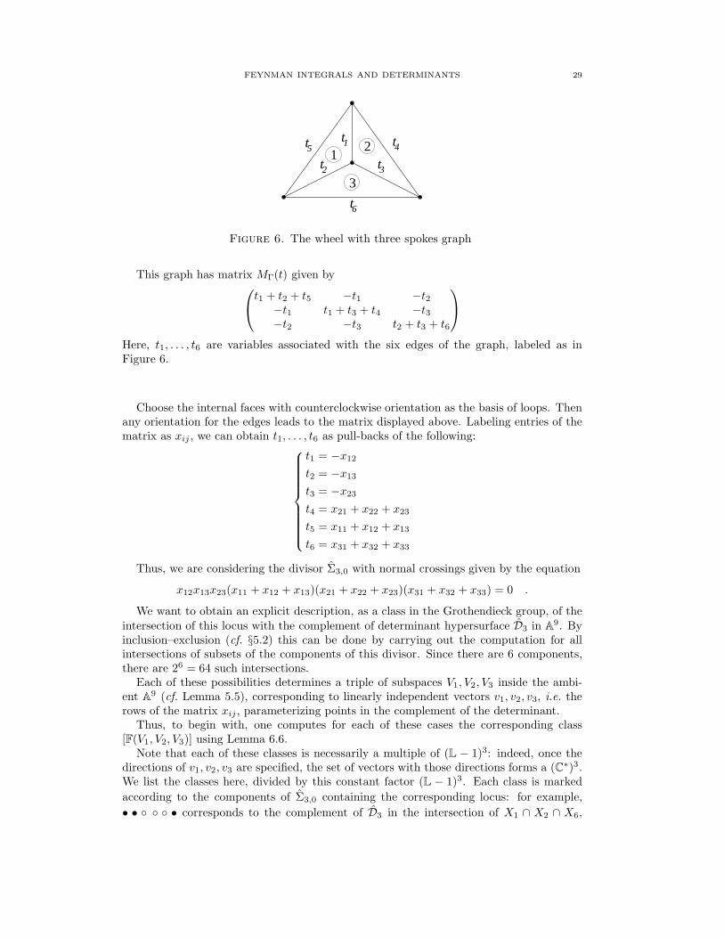
FEYNMAN INTEGRALS AND DETERMINANTS 29
5t4
t6
t2
t1
t31
2
3
t
Figure 6. The wheel with three spokes graph
This graph has matrix MΓ(t) given by
t1 + t2 + t5 −t1 −t2−t1 t1 + t3 + t4 −t3−t2 −t3 t2 + t3 + t6
Here, t1, . . . , t6 are variables associated with the six edges of the graph, labeled as inFigure 6.
Choose the internal faces with counterclockwise orientation as the basis of loops. Thenany orientation for the edges leads to the matrix displayed above. Labeling entries of thematrix as xij , we can obtain t1, . . . , t6 as pull-backs of the following:
t1 = −x12
t2 = −x13
t3 = −x23
t4 = x21 + x22 + x23
t5 = x11 + x12 + x13
t6 = x31 + x32 + x33
Thus, we are considering the divisor Σ3,0 with normal crossings given by the equation
x12x13x23(x11 + x12 + x13)(x21 + x22 + x23)(x31 + x32 + x33) = 0 .
We want to obtain an explicit description, as a class in the Grothendieck group, of theintersection of this locus with the complement of determinant hypersurface D3 in A9. Byinclusion–exclusion (cf. §5.2) this can be done by carrying out the computation for allintersections of subsets of the components of this divisor. Since there are 6 components,there are 26 = 64 such intersections.
Each of these possibilities determines a triple of subspaces V1, V2, V3 inside the ambi-ent A9 (cf. Lemma 5.5), corresponding to linearly independent vectors v1, v2, v3, i.e. therows of the matrix xij , parameterizing points in the complement of the determinant.
Thus, to begin with, one computes for each of these cases the corresponding class[F(V1, V2, V3)] using Lemma 6.6.
Note that each of these classes is necessarily a multiple of (L − 1)3: indeed, once thedirections of v1, v2, v3 are specified, the set of vectors with those directions forms a (C∗)3.We list the classes here, divided by this constant factor (L − 1)3. Each class is marked
according to the components of Σ3,0 containing the corresponding locus: for example,
• • ◦ ◦ ◦ • corresponds to the complement of D3 in the intersection of X1 ∩ X2 ∩ X6,
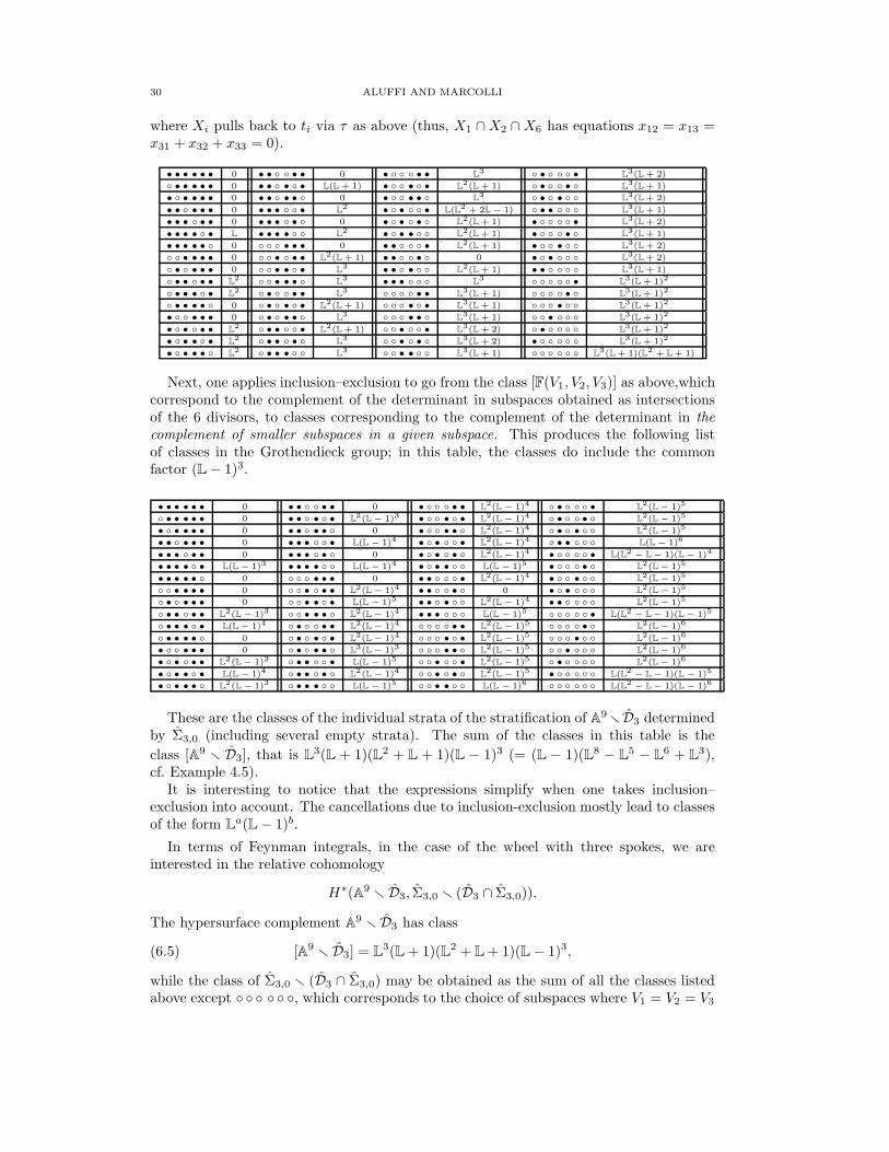
30 ALUFFI AND MARCOLLI
where Xi pulls back to ti via τ as above (thus, X1 ∩ X2 ∩ X6 has equations x12 = x13 =x31 + x32 + x33 = 0).
• • • • • • 0 • • ◦ ◦ • • 0 • ◦ ◦ ◦ • • L3◦ • ◦ ◦ ◦ • L3(L + 2)
◦ • • • • • 0 • • ◦ • ◦ • L(L + 1) • ◦ ◦ • ◦ • L2(L + 1) ◦ • ◦ ◦ • ◦ L3(L + 1)
• ◦ • • • • 0 • • ◦ • • ◦ 0 • ◦ ◦ • • ◦ L3◦ • ◦ • ◦ ◦ L3(L + 2)
• • ◦ • • • 0 • • • ◦ ◦ • L2• ◦ • ◦ ◦ • L(L2 + 2L − 1) ◦ • • ◦ ◦ ◦ L3(L + 1)
• • • ◦ • • 0 • • • ◦ • ◦ 0 • ◦ • ◦ • ◦ L2(L + 1) • ◦ ◦ ◦ ◦ • L3(L + 2)
• • • • ◦ • L • • • • ◦ ◦ L2• ◦ • • ◦ ◦ L2(L + 1) • ◦ ◦ ◦ • ◦ L3(L + 1)
• • • • • ◦ 0 ◦ ◦ ◦ • • • 0 • • ◦ ◦ ◦ • L2(L + 1) • ◦ ◦ • ◦ ◦ L3(L + 2)
◦ ◦ • • • • 0 ◦ ◦ • ◦ • • L2(L + 1) • • ◦ ◦ • ◦ 0 • ◦ • ◦ ◦ ◦ L3(L + 2)
◦ • ◦ • • • 0 ◦ ◦ • • ◦ • L3• • ◦ • ◦ ◦ L2(L + 1) • • ◦ ◦ ◦ ◦ L3(L + 1)
◦ • • ◦ • • L2◦ ◦ • • • ◦ L3
• • • ◦ ◦ ◦ L3◦ ◦ ◦ ◦ ◦ • L3(L + 1)2
◦ • • • ◦ • L2◦ • ◦ ◦ • • L3
◦ ◦ ◦ ◦ • • L3(L + 1) ◦ ◦ ◦ ◦ • ◦ L3(L + 1)2
◦ • • • • ◦ 0 ◦ • ◦ • ◦ • L2(L + 1) ◦ ◦ ◦ • ◦ • L3(L + 1) ◦ ◦ ◦ • ◦ ◦ L3(L + 1)2
• ◦ ◦ • • • 0 ◦ • ◦ • • ◦ L3◦ ◦ ◦ • • ◦ L3(L + 1) ◦ ◦ • ◦ ◦ ◦ L3(L + 1)2
• ◦ • ◦ • • L2◦ • • ◦ ◦ • L2(L + 1) ◦ ◦ • ◦ ◦ • L3(L + 2) ◦ • ◦ ◦ ◦ ◦ L3(L + 1)2
• ◦ • • ◦ • L2◦ • • ◦ • ◦ L3
◦ ◦ • ◦ • ◦ L3(L + 2) • ◦ ◦ ◦ ◦ ◦ L3(L + 1)2
• ◦ • • • ◦ L2◦ • • • ◦ ◦ L3
◦ ◦ • • ◦ ◦ L3(L + 1) ◦ ◦ ◦ ◦ ◦ ◦ L3(L + 1)(L2 + L + 1)
Next, one applies inclusion–exclusion to go from the class [F(V1, V2, V3)] as above,whichcorrespond to the complement of the determinant in subspaces obtained as intersectionsof the 6 divisors, to classes corresponding to the complement of the determinant in thecomplement of smaller subspaces in a given subspace. This produces the following listof classes in the Grothendieck group; in this table, the classes do include the commonfactor (L − 1)3.
• • • • • • 0 • • ◦ ◦ • • 0 • ◦ ◦ ◦ • • L2(L − 1)4 ◦ • ◦ ◦ ◦ • L2(L − 1)5
◦ • • • • • 0 • • ◦ • ◦ • L2(L − 1)3 • ◦ ◦ • ◦ • L2(L − 1)4 ◦ • ◦ ◦ • ◦ L2(L − 1)5
• ◦ • • • • 0 • • ◦ • • ◦ 0 • ◦ ◦ • • ◦ L2(L − 1)4 ◦ • ◦ • ◦ ◦ L2(L − 1)5
• • ◦ • • • 0 • • • ◦ ◦ • L(L − 1)4 • ◦ • ◦ ◦ • L2(L − 1)4 ◦ • • ◦ ◦ ◦ L(L − 1)6
• • • ◦ • • 0 • • • ◦ • ◦ 0 • ◦ • ◦ • ◦ L2(L − 1)4 • ◦ ◦ ◦ ◦ • L(L2− L − 1)(L − 1)4
• • • • ◦ • L(L − 1)3 • • • • ◦ ◦ L(L − 1)4 • ◦ • • ◦ ◦ L(L − 1)5 • ◦ ◦ ◦ • ◦ L2(L − 1)5
• • • • • ◦ 0 ◦ ◦ ◦ • • • 0 • • ◦ ◦ ◦ • L2(L − 1)4 • ◦ ◦ • ◦ ◦ L2(L − 1)5
◦ ◦ • • • • 0 ◦ ◦ • ◦ • • L2(L − 1)4 • • ◦ ◦ • ◦ 0 • ◦ • ◦ ◦ ◦ L2(L − 1)5
◦ • ◦ • • • 0 ◦ ◦ • • ◦ • L(L − 1)5 • • ◦ • ◦ ◦ L2(L − 1)4 • • ◦ ◦ ◦ ◦ L2(L − 1)5
◦ • • ◦ • • L2(L − 1)3 ◦ ◦ • • • ◦ L2(L − 1)4 • • • ◦ ◦ ◦ L(L − 1)5 ◦ ◦ ◦ ◦ ◦ • L(L2− L − 1)(L − 1)5
◦ • • • ◦ • L(L − 1)4 ◦ • ◦ ◦ • • L2(L − 1)4 ◦ ◦ ◦ ◦ • • L2(L − 1)5 ◦ ◦ ◦ ◦ • ◦ L2(L − 1)6
◦ • • • • ◦ 0 ◦ • ◦ • ◦ • L2(L − 1)4 ◦ ◦ ◦ • ◦ • L2(L − 1)5 ◦ ◦ ◦ • ◦ ◦ L2(L − 1)6
• ◦ ◦ • • • 0 ◦ • ◦ • • ◦ L3(L − 1)3 ◦ ◦ ◦ • • ◦ L2(L − 1)5 ◦ ◦ • ◦ ◦ ◦ L2(L − 1)6
• ◦ • ◦ • • L2(L − 1)3 ◦ • • ◦ ◦ • L(L − 1)5 ◦ ◦ • ◦ ◦ • L2(L − 1)5 ◦ • ◦ ◦ ◦ ◦ L2(L − 1)6
• ◦ • • ◦ • L(L − 1)4 ◦ • • ◦ • ◦ L2(L − 1)4 ◦ ◦ • ◦ • ◦ L2(L − 1)5 • ◦ ◦ ◦ ◦ ◦ L(L2− L − 1)(L − 1)5
• ◦ • • • ◦ L2(L − 1)3 ◦ • • • ◦ ◦ L(L − 1)5 ◦ ◦ • • ◦ ◦ L(L − 1)6 ◦ ◦ ◦ ◦ ◦ ◦ L(L2− L − 1)(L − 1)6
These are the classes of the individual strata of the stratification of A9 r D3 determinedby Σ3,0 (including several empty strata). The sum of the classes in this table is the
class [A9 r D3], that is L3(L + 1)(L2 + L + 1)(L − 1)3 (= (L − 1)(L8 − L5 − L6 + L3),cf. Example 4.5).
It is interesting to notice that the expressions simplify when one takes inclusion–exclusion into account. The cancellations due to inclusion-exclusion mostly lead to classesof the form La(L − 1)b.
In terms of Feynman integrals, in the case of the wheel with three spokes, we areinterested in the relative cohomology
H∗(A9 r D3, Σ3,0 r (D3 ∩ Σ3,0)).
The hypersurface complement A9 r D3 has class
(6.5) [A9 r D3] = L3(L + 1)(L2 + L + 1)(L − 1)3,
while the class of Σ3,0 r (D3 ∩ Σ3,0) may be obtained as the sum of all the classes listedabove except ◦ ◦ ◦ ◦ ◦ ◦, which corresponds to the choice of subspaces where V1 = V2 = V3

FEYNMAN INTEGRALS AND DETERMINANTS 31
2 t3
t5 t4
t1
1 2
3t
Figure 7. Another graph with 3 loops and injective τ
is the whole space (these are all the strata of Σ3,0 r (D3 ∩ Σ3,0)) or, equivalently, thedifference of (6.5) and the last item ◦ ◦ ◦ ◦ ◦ ◦. This gives
[Σ3,0 r (D3 ∩ Σ3,0)] = L3(L + 1)(L2 + L + 1)(L − 1)3 − L(L2 − L − 1)(L − 1)6
= L(6L4 − 3L3 + 2L2 + 2L − 1)(L − 1)3
The main information is carried by the class ◦ ◦ ◦ ◦ ◦ ◦,
(6.6) L(L2 − L − 1)(L − 1)6.
In the case of other 3-loop graphs Γ, such as the one illustrated in Figure 7, the divisorΣΓ is a union of components of Σ3,0 (cf. Proposition 5.2). The class of the locus ΣΓ r
(D3 ∩ Σ3,0) may be obtained by adding up all contributions listed above, for the strata
contained in ΣΓ. For the example given in Figure 7, these are the strata contained in thedivisors X1, . . . , X5; the corresponding classes are those marked by ∗ ∗ ∗ ∗ ∗ ∗, where atleast one of the first five ∗ is •; or, equivalently, the difference of (6.5) and the classesmarked ◦ ◦ ◦ ◦ ◦ • and ◦ ◦ ◦ ◦ ◦ ◦. The sum of these two classes is
L(L2 − L − 1)(L − 1)5 + L(L2 − L − 1)(L − 1)6 = L2(L2 − L − 1)(L − 1)5
(cf. (6.6)), and hence
[ΣΓ r (D3 ∩ Σ3,0)] = L3(L + 1)(L2 + L + 1)(L − 1)3 − L2(L2 − L − 1)(L − 1)5
= L2(5L3 + 1)(L − 1)3 .
7. Divergences and renormalization
Our analysis in the previous sections of this paper concentrated on the task of showingthat a certain relative cohomology is a realization of a mixed Tate motive m(X, Y ), wherethe loci X and Y are constructed, respectively, as the complement of the determinanthypersurface and the intersection with this complement of a normal crossing divisor thatcontains the image of the boundary of the domain of integration σn under the map τΓ,for any graph Γ with fixed number of loops and fixed genus. Knowing that m(X, Y ) is amixed Tate motive implies that, when convergent, the parametric Feynman integral for allsuch graphs is a period of a mixed Tate motive. This, however, does not take into accountthe presence of divergences in the Feynman integrals.
There are several different approaches to regularize and renormalize the divergent in-tegrals. We outline here some of the possibilities and comment on how they can be madecompatible with our approach.
32 ALUFFI AND MARCOLLI
7.1. Blowups. One possible approach to dealing with divergences coming from the in-tersections of the divisor Σn with the graph hypersurface XΓ is the one proposed byBloch–Esnault–Kreimer in [10], namely one can proceed to perform a series of blowupsof strata of this intersection until one has separated the domain of integration from thehypersurface and in this way regularized the integral.
In our setting, a similar approach should be reformulated in the ambient Aℓ2 and in
terms of the intersection of the determinant hypersurface Dℓ with the divisor Σℓ,g. If themain question posed in §5.3 has an affirmative answer, then this intersection admits astratification by mixed Tate nonsingular loci. It seems likely that a suitable sequence ofblow-ups would then have the effect of regularizing the integral, while at the same timemaintaining the motivic nature of the relevant loci unaltered. We intend to return to amore detailed analysis of this approach in future work.
7.2. Dimensional regularization and L-functions. Belkale and Brosnan showed in[4] that dimensionally regularized Feynman integrals can be written in the form of alocal Igusa L-function, where the coefficients of the Laurent series expansion are periods,provided the integrals describing them are convergent. Such periods have an explicitdescription in terms of integrals on simplices σn and cubes [0, 1]r of algebraic differentalforms
f(t)s0ωn ∧f(t) − 1
(f(t) − 1)t1 + 1dt1 ∧ · · · ∧
f(t) − 1
(f(t) − 1)tr + 1dtr,
for f(t) = ΨΓ(t) the graph polynomial. The nature of such integrals as periods wouldstill be controlled by the same motivic loci that are involved in the original parametricFeynman integral before dimensional regularization. The result of [4] is formulated onlyfor the case of log-divergent integrals where only the graph polynomial ΨΓ(t) is present inthe Feynman parametric form and not the polynomial PΓ(t, p). The result was extendedto the more general non-log-divergent case by Bogner and Weinzierl in [12].
In this approach, if there are singularities in the integrals that compute the coeffientsof the Laurent series expansion of the local Igusa L-function giving the dimensionallyregularized Feynman integral, these can be treated by an algorithmic procedure developedby Bogner and Weinzierl in [13] (see also the short survey [14]). The algorithm is designedto split the divergent integral into sectors where a change of variable that introducesa blowup at the origin isolates the divergence as a pole in a parameter 1/ǫ. One canthen do a subtraction of this polar part in the Laurent series expansion in the variable ǫand eliminate the divergence. The iteration part of the algorithm is based on Hironaka’spolyhedral game and it is shown in [13] that the resulting algorithm terminates in finitetime.
If one uses this approach in our context one will have to show that the changes ofvariables introduced in the process of evaluating the integrals in sectors do not alter themotivic nature of the loci involved.
7.3. Deformations. An alternative to the use of blowups is the use of deformations. Wediscuss here the simplest possible procedure one can think of that uses deformations of thegraph hypersurface (or of the determinant hypersurface). It is not the most satisfactorydeformation method, because it does not lead immediately to a “minimal subtraction”procedure, but it suffices here to illustrate the idea.
Consider the original parametric Feynman integral of the form
(7.1)
∫
σn
PΓ(t, p)βωn
ΨΓ(t)α,
FEYNMAN INTEGRALS AND DETERMINANTS 33
with exponents α and β as in (1.2),
α = −n + (ℓ + 1)D/2, β = −n + Dℓ/2.
Again, for our purposes, we can assume to work in the “stable range” where D is sufficientlylarge so that both α and β are positive. The case of small D, which is of direct physicsinterest, leads one to the different problem of considering the hypersurfaces defined byPΓ(t, p), as a function of the external momenta p and the singularities produced by theintersections of these with the domain of integration. This type of analysis can be foundin the physics literature, for instance in [32]. See also [7], §18.
Assuming to work in the range where α and β are positive, one can choose to regularizethe integral (7.1) by introducing a deformation parameter ǫ ∈ C r R+ and replaing (7.1)with the deformed
(7.2)
∫
σn
PΓ(t, p)βωn
(ΨΓ(t) − ǫ)α.
This has the effect of replacing, as locus of the singularities of the integrand, the graphhypersurface XΓ = {ΨΓ(t) = 0}, with the level set XΓ,ǫ = {ΨΓ(t) = ǫ} of the map
ΨΓ : An → A. For a choice of ǫ in the cut plane C r R+, the hypersurface XΓ,ǫ does notintersect the domain of integration σn. In fact, for ti ≥ 0 one has ΨΓ(t) ≥ 0. This choicehas therefore the effect of desingularizing the integral. The resulting function of ǫ extendsholomorphically to a function on C r I, where I ⊂ R+ is the bounded interval of valuesof ΨΓ on σn.
When we transform the parametric integral using the map τΓ into an integral of a
form defined on the complement of the determinant hypersurface Dℓ in Aℓ2 on a domainof integration τΓ(σn) with boundary on the divisor Σℓ,g, we can similarly separate the
divisor from the hypersurface by the same deformation, where instead of the locus Dℓ ={det(x) = 0} one considers the level set Dℓ,ǫ = {det(x) = ǫ}, so that Dℓ,ǫ does notintersect τΓ(σn). The nature of the period described by the deformed integral is then
controlled by the motive m(Xǫ, Yǫ) for Xǫ = Aℓ2 r Dℓ,ǫ and Yǫ = Σℓ,g r (Dℓ,ǫ ∩ Σℓ,g). Thequestion becomes then whether the motivic nature of m(X, Y ) with X = X0 and Y = Y0
and m(Xǫ, Yǫ) is the same. This in general is not the case, as one can easily constructexamples of fibrations where the generic fiber is not a mixed Tate motive while the specialone is. However, in this setting one is dealing with a very special case, where the deformedvariety Dℓ,ǫ is given by matrices of fixed determinant. Up to a rescaling, one can check
that the fiber Dℓ,1 = SLn is indeed a mixed Tate motive, from the general results of Biglari[5], [6] on reductive groups. Thus, over a set of algebraic values of ǫ one does not leave theworld of mixed Tate motives. This will give a statement on the nature of the regularizedFeynman integrals as a period of a mixed Tate motive m(Xǫ, Yǫ) and reduces then theproblem to that of removing the divergence as ǫ → 0, in such a way that what remains is aconvergent integral whose nature as a period is controlled by the original motive m(X, Y ).
A different approach to the regularization of parametric Feynman integrals using de-formations was discussed in [25] in terms of Leray cocycles and a related regularizationprocedure.
Acknowledgment. The first author is partially supported by NSA grant H98230-07-1-0024. The second author is partially supported by NSF grant DMS-0651925. This workwas partly carried out during stays of the authors at the MPI and MSRI. The first authoralso thanks the California Institute of Technology, where part of this work was done.
References
[1] P. Aluffi, M. Marcolli, Feynman motives of banana graphs. preprint arXiv:hep-th/0807.1690.

34 ALUFFI AND MARCOLLI
[2] P. Aluffi, M. Marcolli, Algebro-geometric Feynman rules, preprint arXiv:0811.2514.[3] P. Belkale, P. Brosnan, Matroids, motives, and a conjecture of Kontsevich, Duke Math. Journal,
Vol.116 (2003) 147–188.[4] P. Belkale, P. Brosnan, Periods and Igusa local zeta functions. Int. Math. Res. Not. 2003, no.
49, 2655–2670.[5] S. Biglari, Motives of reductive groups, PhD Thesis, University of Leipzig, 2004.[6] S. Biglari, On the cohomology of the motive of a reductive group, preprint 2008.[7] J. Bjorken, S. Drell, Relativistic Quantum Mechanics, McGraw-Hill, 1964, and Relativistic Quan-
tum Fields, McGraw-Hill, 1965.[8] S. Bloch, Lectures on mixed motives. Algebraic geometry—Santa Cruz 1995, 329–359, Proc.
Sympos. Pure Math., 62, Part 1, Amer. Math. Soc., 1997.[9] S. Bloch, Motives associated to graphs, Japan J. Math., Vol.2 (2007) 165–196.
[10] S. Bloch, E. Esnault, D. Kreimer, On motives associated to graph polynomials, Commun. Math.Phys., Vol.267 (2006) 181–225.
[11] S. Bloch, D. Kreimer, Mixed Hodge structures and renormalization in physics, arXiv:0804.4399.[12] C. Bogner, S. Weinzierl, Periods and Feynman integrals, arXiv:0711.4863.[13] C. Bogner, S. Weinzierl, Resolution of singularities for multi-loop integrals, arXiv:0709.4092.[14] C. Bogner, S. Weinzierl, Blowing up Feynman integrals, arXiv:0806.4307.[15] D. Broadhurst, D. Kreimer, Association of multiple zeta values with positive knots via Feynman
diagrams up to 9 loops, Phys. Lett. B, Vol.393 (1997) 403–412.[16] I.M. Gelfand, V.V. Serganova, Combinatorial geometries and the strata of a torus on homoge-
neous compact manifolds. Uspekhi Mat. Nauk 42 (1987), no. 2(254), 107–134, 287.[17] I.M. Gelfand, R.M. Goresky, R.D. MacPherson, V.V. Serganova, Combinatorial geometries,
convex polyhedra, and Schubert cells. Adv. in Math. 63 (1987), no. 3, 301–316.[18] A.B. Goncharov, Periods and mixed Tate motives. preprint arXiv:math.AG/0202154.
[19] A.B. Goncharov, Yu.I. Manin, Multiple ζ-motives and moduli spaces M0,n. Compos. Math. 140(2004), no. 1, 1–14.
[20] H. Grosse, R. Wulkenhaar, Renormalization of noncommutative quantum field theory, pp.129–168, in “An Invitation to Noncommutative Geometry” (Eds. M. Khalkhali, M. Marcolli) WorldScientific, 2008.
[21] R. Gurau, V. Rivasseau, Parametric representation of noncommutative field theory, Commun.Math. Phys., Vol.272 (2007) N.3, 811–835.
[22] C. Itzykson, J.B. Zuber, Quantum Field Theory, Dover Publications, 2006.
[23] T. Krajewski, V. Rivasseau, A. Tanasa, Zhituo Wang, Topological Graph Polynomials and Quan-
tum Field Theory, Part I: Heat Kernel Theories, preprint arXiv:0811.0186.[24] M. Levine, Tate motives and the vanishing conjectures for algebraic K-theory. in “Algebraic
K-theory and algebraic topology”, pp.167–188, NATO Adv. Sci. Inst. Ser. C Math. Phys. Sci.,407, Kluwer Acad. Publ., 1993.
[25] M. Marcolli, Motivic renormalization and singularities, preprint arXiv:math-ph/0804.4824.[26] B. Mohar, C. Thomassen, Graphs on surfaces, Johns Hopkins University Press, 2001.[27] N. Nakanishi Graph Theory and Feynman Integrals. Gordon and Breach, 1971.[28] J. Rammer, Quantum field theory of non-equilibrium states, Cambridge University Press, 2007.[29] M. Sato, T. Miwa, M. Jimbo, T. Oshima, Holonomy structure of Landau singularities and
Feynman integrals, Publ. Res. Inst. Math. Sci. Volume 12, Supplement (1976/1977) (1976), 387–439.
[30] B. Shapiro, M. Shapiro, A. Vainshtein, On combinatorics and topology of pairwise intersections of
Schubert cells in SLn/B. in “The Arnold-Gelfand mathematical seminars”, 397–437, Birkhauser,1997.
[31] B. Shapiro, M. Shapiro, A. Vainshtein, Topology of intersections of Schubert cells and Hecke
algebra. Proceedings of the 5th Conference on Formal Power Series and Algebraic Combinatorics(Florence, 1993). Discrete Math. 153 (1996), no. 1-3, 305–318.
[32] I.T. Todorov, Analytic properties of Feynman diagrams in quantum field theory, Pergamon Press,1971.
[33] V. Voevodsky, Triangulated categories of motives over a field. in “Cycles, transfers, and motivichomology theories”, pp.188–238, Ann. of Math. Stud., 143, Princeton Univ. Press, 2000.
Department of Mathematics, Florida State University, Tallahassee, FL 32306, USA
E-mail address: [email protected]
Department of Mathematics, Caltech, Pasadena, CA 91125, USA
E-mail address: [email protected]


![Feynman integrals and multiple polylogarithms arXiv:0705.0900v1 … · arXiv:0705.0900v1 [hep-ph] 7 May 2007 MZ-TH/07-06 Feynman integrals and multiple polylogarithms Stefan Weinzierl](https://img.pdfslide.us/doc/110x75/60546717048db466a451dca9/feynman-integrals-and-multiple-polylogarithms-arxiv07050900v1-arxiv07050900v1.jpg)