Embed Size (px)
Citation preview
Forthcoming Journal of Banking and Finance 25:1, January 2001
Parameterizing Credit Risk ModelsWith Rating Data
Mark Carey*Federal Reserve Board
Mark HrycayAdvertising.com
October 18, 2000
JEL codes: G11, G20, G31, G33Keywords: credit risk, value at risk, credit ratings, debt default, capital regulation
*Corresponding author. Postal mail to Federal Reserve Board, Washington, DC, 20551;(202) 452-2784 (voice); (202) 452-5295 (fax). This paper represents the authors’ opinions andnot necessarily those of the Board of Governors, other members of its staff, or the FederalReserve System. We thank Ed Altman, Lea Carty, Eric Falkenstein, Michael Gordy, DavidJones, Jan Krahnen, John Mingo, Tony Saunders, Andrea Sironi and William Treacy for usefulconversations.
Parameterizing Credit Risk Models With Rating Data
--- Abstract ---
Estimates of average default probabilities for borrowers assigned to each of a financialinstitution’s internal credit risk rating grades are crucial inputs to portfolio credit risk models. Such models are increasingly used in setting financial institution capital structure, in internalcontrol and compensation systems, in asset-backed security design, and are being considered foruse in setting regulatory capital requirements for banks. This paper empirically examinesproperties of the major methods currently used to estimate average default probabilities bygrade. Evidence of potential problems of bias, instability, and gaming is presented. With care,and perhaps judicious application of multiple methods, satisfactory estimates may be possible. In passing, evidence is presented about other properties of internal and rating-agency ratings.
1
1 For example, consider a bank with a portfolio of assets that has a 0.01 probability ofgenerating losses at a 6 percent or higher rate over the upcoming year. If the bank’s capitalstructure involves a ratio of reserves plus equity to assets of 6 percent, and it finds the implied0.01 one-year insolvency probability uncomfortably high, the bank must either raise new equityor rebalance its portfolio such that the chance of large losses is reduced.
Many financial institutions are adopting variants of value at risk (VaR) approaches to
measurement and management of credit risk. In such approaches, an institution estimates
probability distributions of credit losses conditional on portfolio composition. The institution
seeks to choose simultaneously a portfolio and a capital structure such that the estimated
probability is small that credit losses will exceed allocated equity capital.1 In addition to
influencing capital structure and investment strategy, credit risk capital allocations are playing
an increasingly important role in management control and incentive compensation systems (such
as RAROC systems), and bank regulators are considering incorporating VaR concepts in a
redesigned system of capital regulation for credit risk (Basel 1999). VaR approaches are also
used in designing structured securities like collateralized loan obligations (CLOs). Thus, the
quality of estimates of portfolio credit loss distributions is an increasingly important determinant
of many financial decisions.
Several approaches to estimating credit loss distributions are now in use (Ong 1999), but
the credit risk ratings of individual borrowers are always key inputs. A rating summarizes the
risk of credit loss due to failure by the rated counterparty to pay as promised. The most familiar
examples of ratings are those produced by agencies such as Moody’s and Standard & Poor’s
(S&P), but virtually all major U.S. commercial banks and insurance companies and many non-
U.S. financial institutions produce internal ratings for each counterparty or exposure and employ
such ratings in their credit risk modeling and management. Internal rating systems differ across
institutions in terms of numbers of grades and other features, and are likely to continue to differ
from each other and from rating agency systems (Treacy and Carey 1998, briefly summarized in
Appendix A; English and Nelson 1999; Krahnen and Weber 2000). Ratings matter because they
proxy for default probabilities of individual borrowers and such probabilities materially
influence portfolio credit risk (in contrast to equity portfolios, both cross-asset return
correlations and individual-asset risk affect portfolio bad-tail risk even for large debt portfolios--
2
2 Many internal ratings incorporate considerations of loss given default (LGD) as well asprobability of default. Estimating average default probabilities for such ratings involvescomplexities we do not address, in part because institutions making heavy use of credit riskmodels often change their rating systems to include obligor or pure default grades.
3 Evidence presented below indicates that a relatively long time series of data is neededfor good actuarial estimates. Thus, for many banks, an ability to rely completely on internal datamay be many years in the future even if appropriate data warehousing were to beginimmediately. Even in cases where banks have gathered such data, changes in the architecture orcriteria of their internal rating system (which occur frequently) greatly reduce the utility of pre-change data. Thus, the methods of quantification analyzed in this paper are likely to be usedindefinitely.
-see Appendix A).
Ratings are usually recorded on an ordinal scale and thus are not directly usable measures
of default probability.2 Thus, a crucial step in implementing portfolio credit risk models or
capital allocation systems is estimation of the (natural) probability of default for counterparties
assigned to each grade (hereafter referred to as “rating quantification”). Remarkably, very few
financial institutions have maintained usable records of default and loss experience by internal
grade for their own portfolios. Thus, the obvious actuarial approach, computing long-run
average default rates from the historical experience of borrowers in each internal grade, is not
feasible in most cases.3
Instead, most institutions use one of two methods that are based on external data. The
most popular such method involves mapping each internal grade to a grade on the Moody’s or
Standard & Poor’s (S&P) scale and using the long-run average default rate for the mapped
agency grade to quantify the internal grade. The mapping method is popular because of its
apparent simplicity, because agency grades are familiar to most market participants, and because
Moody’s and S&P maintain databases with long histories of default experience for publicly
issued bonds and regularly publish tables of historical average default rates.
Commercial credit scoring models are the basis for the second commonly used method of
quantifying ratings. Scoring models produce estimated default probabilities (or other risk
measures) for individual borrowers, typically using borrower financial ratios and other
characteristics as predictors. Where a model can produce fitted default probabilities for a
representative sample of borrowers in each internal grade, averages of the fitted values may be
3
used as estimates of average default probabilities for each grade.
In spite of their popularity, the properties of mapping- and scoring-model-based methods
of rating quantification are not well understood. This paper is the first systematic analysis of
such properties. The closest extant work seems to be Falkenstein (2000), Delianis and Geske
(1999), and Nickell, Perraudin and Varotto (2000). Many papers have appeared on the relative
merits of different credit scoring models as predictors of individual defaults (see Altman and
Saunders (1998), Falkenstein (2000), and Sobehart, Keenan and Stein (2000) for references), but
we focus on prediction of the proportion of borrowers defaulting in each grade. It is possible
that methods optimized to predict individual defaults may not perform well in quantifying
grades, and vice versa.
Our empirical evidence implies that, while mapping and scoring-model methods are each
capable of delivering reasonably accurate estimates, apparently minor variations in method can
cause results to differ by as much as an order of magnitude. When realistic variations in average
default probabilities by grade are run through a typical capital allocation model as applied to a
typical large U.S. bank portfolio, the implied equity capital allocation ratio can change by
several percentage points, which represents a very large economic effect of potential
measurement errors in quantification.
Our analysis focuses on issues of bias, stability, and gaming. Two kinds of bias specific
to rating quantification may affect both mapping- and scoring-model-based quantifications even
in the absence in instabilities or gaming. A “noisy-rating-assignments bias” arises as a by-
product of the bucketing process inherent in rating assignment. Explicitly or implicitly, both
rating assignment and quantification involve estimation of individual borrower default
probabilities as an intermediate step. Even where such estimates for individual borrowers are
unbiased overall, the act of using them to place borrowers in rating buckets tends to create a
variant of selection bias, concentrating negative rating assignment probability errors in the safe
grades and positive errors in the risky grades. When noise in rating assignment probabilities and
rating quantification probabilities is correlated, actual default rates are likely to be higher than
estimated by the method of quantification for the safe grades and lower than estimated for the
risky grades.
An “informativeness” bias arises when the method of quantification produces individual
4
borrower default probability estimates that do not perfectly distinguish relatively safe or risky
borrowers from the average borrower. Where such individual-borrower probabilities are biased
toward the portfolio mean probability (probably the most common case), informativeness bias
tends to make actual default rates smaller than estimated for the safe grades and larger than
estimated for the risky grades. Thus, in many cases, noisy-rating-assignment bias and
informativeness bias tend to offset
Though the net bias in any given case is sensitive to details of the rating system and
method of quantification, in our empirical exercises the informativeness bias generally
dominates and can be material for both mapping and scoring model methods. However, median-
based methods seem to work reasonably well for relatively safe grades like the agencies’
investment grades (but poorly for the junk grades), whereas mean-based methods work
reasonably well for the junk grades (and poorly for the investment grades). Thus, in the absence
of instabilities or gaming, both mapping and scoring model methods appear to be capable of
producing reasonably good results if mean- and median-based methods are mixed.
Quantifications are unstable if their accuracy depends materially on the point in time at
which a mapping is done, on the sample period over which scoring-model parameters are
estimated, or if scoring model- or mapping-based estimates of default probabilities are unreliable
out-of-sample. Most internal rating systems’ methods of rating assignment are different from
those of the agencies in ways that might make mappings unstable. Importantly, most U.S. banks
rate a borrower according to its current condition at the point in time the rating is assigned,
whereas the agencies estimate a downside or stress scenario for the borrower and assign their
rating based on the borrower’s projected condition in the event the scenario occurs (a “through-
the-cycle” method). The difference in rating philosophy potentially causes internal and agency
grades to have different cyclical and other properties, but no evidence of the magnitude of the
problem has been available. The difference in rating methods is likely to persist because the
agencies’ method is too expensive to apply to many bank loans and because banks use internal
ratings to guide the intensity of loan monitoring activity, which implies a continuing need for a
point-in-time architecture (see Treacy and Carey 1998).
We find evidence of through-the-cycle versus point-in-time instability mainly for grades
corresponding to A, Baa, and Ba, and then mainly for mean-based mapping methods. However,
5
4 Principal-agent problems might also arise where rating agencies use scoring models inanalyzing the risk of structured instruments like CLOs, or where credit risk models are usedinternally by financial institutions as one determinant of employee compensation.
we find evidence of regime shifts and random instabilities that can materially affect the quality
of mapping-based estimated default probabilities across the credit quality spectrum. Such
instability may be controllable by basing mappings on several years of pooled data, but more
research is needed.
An advantage of the scoring model method is that scoring model architecture and
forecasting horizon can be tailored to conform to typical point-in-time internal rating systems,
and thus cyclical instability of the sort that can affect mappings should not be a problem. More
conventional out-of-sample instability of estimates also does not appear to be a problem for the
scoring model we use, but we present evidence that models estimated with only a few years of
data may be unstable. Thus, some scoring models may be preferred to others for stability
reasons.
Multiple parties may use the quantification for a given internal rating system and
sometimes those producing the quantification may have incentives to deliberately distort or
“game” results in order to make others believe the portfolio is less risky than is actually the case.
For example, if regulators were to use quantifications of banks’ internal grades in setting
regulatory capital requirements, some banks might draw the boundaries of internal rating grades
in a manner that reduced estimated probabilities produced by median-based mappings. We
present evidence that such gaming can be material, raising actual default rates relative to
estimates by a factor of two or more for each internal grade. However, gaming of median-based
mappings appears to be controllable at relatively modest cost with appropriate monitoring.
A bank might also game quantifications by altering its portfolio investment strategies to
exploit limitations in the information set used by the quantification method. For example,
investments might be focused in relatively high-risk loans that a scoring model fails to identify
as high-risk, leading to an increase in actual portfolio risk but no increase in the bank’s estimated
capital allocations.4
We provide a conservative estimate of the possible size of distortions from information-
based gaming by simulating default rates from gamed and ungamed portfolio investment
6
strategies. Distortions can be material, with simulated gamed-portfolio default rates for each
grade two or more times larger than ungamed rates for all but the riskiest internal grade. This
sort of gaming may be more difficult to detect than gaming by adjusting internal rating scale
boundaries, especially where a scoring model is the basis for quantification.
Taken as a whole, our evidence implies that parameterization of credit risk models using
rating data is itself a risky business but one for which the risks are controllable by careful
analysis and management. Casual quantifications can result in large errors in capital allocations.
However, with attention to problems of bias, stability and gaming and with more research,
reasonably good estimates of average default probabilities by grade appear feasible.
A principal current challenge to empirical work is the absence of data on internal rating
assignments and associated borrower characteristics and defaults. We sidestep this problem by
simulating internal ratings. We estimate logit models of default probability for a large sample of
U.S. bond issuers, assigning each borrower in each year to a simulated internal grade based on
its fitted default probability. Because our goal is not to produce the best scoring model but
rather to evaluate methods of rating quantification, we deliberately use very simple models and
are careful not to overfit the data. We examine the out-of-sample accuracy of estimated average
default rates by both simulated grade and Moody’s grade as produced by both the scoring model
and the mapping method. Our results indicate that properties of different quantification methods
can vary with details of the internal rating system to be quantified and of any scoring model that
is used. Thus, empirical analysis of actual internal rating data, when it becomes available, is
very desirable.
Our evidence represents a first step toward understanding and reliable practice. In
addition to limitations associated with simulated internal ratings, other data limitations cause us
to analyze only default risk, not risk associated with changes in spreads or changes in borrower
credit quality short of default. Rating transition matrices are a common basis for modeling the
latter, and Krahnen and Weber (2000) present evidence that transition rates are much higher for
point-in-time internal rating systems than for agency ratings. Our simulated point-in-time
internal grades also have higher transition rates.
Some portfolio models require as inputs measures of the volatility of default rates (Gordy
2000b) and such volatility is commonly measured using rating agency default rate histories,
7
5 We thank Michael Gordy and John Mingo for this point.
which might have different volatility properties than internal ratings. Although our evidence is
only indicative, we find annual default rate volatility to be rather similar for agency grades and
our simulated internal grades.
Some of the issues we raise regarding rating quantification are most applicable to credit
risk measurement for commercial loan and other private debt portfolios. For specialty portfolios
or portfolios of small consumer or business loans, the mapping method may be inappropriate
because such loans may behave differently than large corporate loans. For rated bond portfolios,
quantification is easier because the agencies’ actuarial estimates of default probabilities by grade
may be used. For portfolios of actively traded instruments, methods of credit risk analysis that
extract information from spreads are appealing. Such methods often focus on risk-neutral
default probabilities rather than the natural probabilities of this paper. However, satisfactory
data are generally not available to support such methods even for portfolios of straight public
debt, and moreover most bank counterparties are private firms.
Although current credit risk modeling practice involves use of estimated long-run
average probabilities of default or transition that are not conditional on the current state of the
economy or on predictable variations in other systematic credit risk factors, extant credit risk
models implicitly assume that input probabilities are conditioned on such factors.5 We follow
current practice in focusing on unconditional or long-run averages, but methods of producing
conditional estimates and of incorporating the possibility of quantification error in portfolio
model specifications are important subjects for future research.
For simplicity, all types of financial institutions are hereafter denoted “banks.” Section 1
presents a simple conceptual framework and associated notation that are useful in analyzing bias
and stability, describes available methods of quantification in more detail, and presents the plan
of empirical analysis. Section 2 describes the data, while Section 3 presents the simple scoring
model and describes how we simulate internal rating assignments. Section 4 presents evidence
about bias, in the process producing examples of both mapping- and scoring model-based
quantifications. Section 5 presents evidence about the stability of each method’s estimates, and
also describes the difference in through-the-cycle and point-in-time rating architectures in more
8
6 An example is Texaco’s Chapter 11 filing as part of its strategy in the lawsuit broughtagainst it by Penzoil.
detail. Section 6 provides evidence about the potential severity of gaming-related distortions.
Section 7 presents some indicative evidence about the number of years of data required for
reasonably confident application of actuarial methods, and Section 8 presents indicative
evidence about the impact of bias, stability, and gaming problems on capital requirements for a
typical large U.S. bank loan portfolio. Section 9 concludes with preliminary recommendations
for rating quantification practice and future research.
1. A simple framework, and background
We require a framework of concepts and notation that aids discussion of the dynamic and
long-run average relationships between true probabilities of counterparty default, the estimated
probabilities produced (often implicitly) during the internal rating assignment process, and the
estimated probabilities produced by the quantification method. We adopt some of the concepts
but not necessarily the machinery of standard contingent claim approaches to default risk.
Suppose each borrower i at date t is characterized by a distance from default Dit and a volatility
of that distance Vit. At t, the (unobservable) probability the borrower will default over an n-
year horizon is the probability that Dit evolves to a value of zero sometime during the [t,t+n] time
interval. In the standard contingent-claim approach, Dit is the market value of the borrower’s
assets relative to some value at which default occurs. Asset value evolves stochastically
according to a specification in which asset value volatility is of central importance. Other
approaches to credit analysis focus on the adequacy of the borrower’s cash flow and readily
saleable assets to cover debt service and other fixed charges. In such approaches, Dit might be a
fixed-charge coverage ratio and Vit a volatility of the coverage ratio. In either approach, the Dit
process might have a jump component because relatively healthy borrowers sometimes default.6
A rating system designed to measure default risk over an n-year horizon includes a
means of aggregating information about D and V into (perhaps implicit) default probability
estimates = fn(Dit,Vit) and a rating scale that specifies the grade associated with any
value of . If measures the true probability without error, then all borrowers assigned
9
7 is necessary for . The associated heteroskedasticity of is not a problem for this paper.
8 As described below, in some cases an estimated median may be a better estimator ofthe mean than is an estimated mean.
to a given grade have values within the grade’s defining range of default probability values
(Figure 1 left panel). With measurement error, for example
(1)
the true values for some borrowers in each grade will lie outside the band for the grade
(Figure 1 right panel).7
Human judgement often plays a role in rating assignment. Thus, often is implicit
and unobservable (the true is always unobservable). To quantify average default
probabilities by grade, observable estimates of individual counterparty default probabilities
(2)
are required. In general, the are separate from any produced in the rating process---where
produced by the rating process are observable, is possible, but we do not wish to
restrict attention to that case. Regardless of the source of estimates, it is intuitive that a mean of
one and low variance are desirable characteristics of , but good estimates of average
probabilities for each grade are also needed. Within-grade biases that average to zero across all
grades are problematic because, in estimating portfolio expected and unexpected credit loss
rates, average default probabilities in effect are multiplied by LGD, correlation, and exposure
factors that may differ by grade (see Appendix A).
In current portfolio modeling practice, individual borrower default probability estimates
are usually set to the estimated average probability for the grade to which they are assigned.
Moreover, the estimated average is presumed to correspond to a true mean value, which is a
reasonable predictor of the default rate for the grade. Thus, a primary focus of this paper is
elucidation of the circumstances under which the available methods yield that are stable,
unbiased, low-variance estimators of true means, i.e. whether E( ) = for all grades g and
dates t.8 Such elucidation involves analysis of the dynamic and long-run average relationships
between , , and for any given rating system r and quantification method q.
10
Table 1 summarizes the paper’s notation.
1.1 Variants of scoring model and mapping methods and their weaknesses
Statistical models that estimate default probabilities for individual borrowers may be
used to obtain an estimate of the mean default probability for a grade by averaging model fitted
values for a sample of within-grade borrowers. Any of the mean, the median, or a trimmed
measure of the central tendency of fitted values for a grade may be used as the estimate. Scoring
models may also be used to assign ratings, but a scoring model can be used to quantify any
system of ratings regardless of the manner of their assignment. Advantages of scoring models
include their mechanical nature and the fact that the time horizon and architecture of the model
can be made compatible with that of the rating system or the portfolio credit risk model.
Disadvantages include a requirement that machine-readable data for variables in the model be
available for a sufficiently large and representative sample of borrowers in each grade, the
possibility of poor estimates because the model produces biased or noisy fitted values, and the
possibility of distortions due to principal-agent problems (“gaming”).
Both median-borrower and weighted-mean-default-rate methods of mapping are
available. The median-borrower method involves two stages: 1) equate each internal grade to an
external party’s grade, usually a Moody’s or S&P grade, and 2) use the long-run average default
rate for the mapped external grade as the estimated average default probability for the
internal grade. The first stage may be done judgmentally, by comparing the rating criteria for
the internal grade to agency criteria, or more mechanically, by tabulating the grades of individual
agency-rated credits in each internal grade and taking the rating of the median borrower as
representative of the average risk posed by the grade. The second stage is a straightforward
exercise of reading long-run average default rates from tables in the agencies’ published studies.
The weighted-mean mapping method is a variant of the mechanical median-borrower
method. for each individual agency-rated borrower in an internal grade is taken to be the
long-run average historical default rate for the borrower’s agency grade. The mean of such rates
for each grade is used as the estimate of . Although estimated probabilities for each
borrower are equally-weighted in computing the mean, the nonlinearities in default rates
described below cause values for borrowers in the riskier agency grades to have a
disproportionate impact on the results of this method.
11
Judgmental median-borrower mappings, though very common, are difficult to implement
with confidence because both the rating agencies’ written rating criteria and especially those for
banks’ internal rating systems are vague (Treacy and Carey 1998). Such mappings usually are
based on the intuition of the bank’s senior credit personnel about the nature of credits in each
agency grade versus each internal grade. Moreover, the fact that agency ratings are based on
stress scenarios whereas bank ratings typically are based on the borrower’s current condition
means that the two sets of rating criteria are potentially incompatible even where they may
appear similar. Only if differences in architecture and moderate differences in rating criteria are
unimportant empirically is the judgmental mapping method likely to be reliable in practice.
Both mechanical mapping methods are subject to possible selection biases.
Such bias may arise if the agency-rated borrowers assigned to an internal grade pose
systematically different default risk than other borrowers assigned that grade, perhaps flowing
from the fact that the agency-rated borrowers tend to be larger and to have access to a wider
variety of sources of finance. There is evidence that such differences in default rates exist, but
the evidence is not yet sufficient to suggest how bond default rates should be adjusted (see
Society of Actuaries (1998) and Altman and Suggitt (2000) for contrasting results). Selection
bias might also arise deliberately—a bank might cause outsiders to underestimate the default risk
of its grades by systematically placing agency-rated borrowers in internal grades that are riskier
than warranted by the borrowers’ characteristics. For example, if the bank placed only agency-
rated Baa borrowers in a grade in which all agency-nonrated borrowers pose Ba levels of risk, an
outsider using mechanical mappings would underestimate default risk for the grade as a whole.
Control of this source of bias appears to require a periodic comparison by outsiders of the
characteristics of a sample of agency-rated and other borrowers in each internal grade.
Users of the both the judgmental and the mechanical methods of mapping face four
additional problems, all of which are described in more detail below: nonlinearities in default
rates by agency grade, model-informativeness and noisy-assignments biases, granularity
mismatches, and problems flowing from through-the-cycle versus point-in-time rating system
architectures.
1.2 Plan of the empirical analysis
Our ability to conduct empirical analysis is limited by the unavailability of two kinds of
12
data: actual internal rating assignments combined with the characteristics of the internally rated
obligors; and a history of default experience for such obligors. Without such data, we cannot
offer empirical evidence about the reliability of judgmental methods of developing internal-to-
agency grade mappings, nor about the importance of differences in riskiness of agency-rated or
credit-scorable borrowers, nor about instabilities flowing from changes in internal rating criteria
over time.
However, obligor ratings, characteristics and default histories are available from
Moody’s for agency-rated U.S. corporations. We use such data to estimate simple models of
borrower default probability and use such models to produce simulated internal rating
assignments. The properties of the simulated ratings are likely to be representative of properties
of internal ratings from systems that use a scoring model similar to ours to make rating
assignments. Some properties may be less similar to those of judgmentally-assigned internal
ratings or those based on very different scoring models---in particular, many internal ratings
embody more information than used in our scoring model---but dynamic properties are likely to
be generally similar in that our scoring model has a one-year horizon and a point-in-time
orientation.
We use one or more of scoring model outputs, the simulated ratings, Moody’s actual
ratings, and historical default rates by simulated and Moody’s grade to shed light on the practical
significance of issues of bias, stability, and gaming for each major method of quantification
(Table 2 summarizes the available quantification methods and the issues).
2. Data
We merge the January, 1999 release of Moody’s Corporate Bond Default Database with
the June, 1999 release of Compustat, which yields a database of Moody’s rated borrowers, their
default histories, and their balance sheet and income statement characteristics for the years 1970-
98. The Moody’s database is a complete history of their long-term rating assignments for both
U.S. and non-U.S. corporations and sovereigns (no commercial paper ratings, municipal bond
ratings, or ratings of asset-backed-securities are included). Ratings on individual bonds as well
as the issuer ratings that are the basis for Moody’s annual default rate studies are included, as are
some bond and obligor characteristics such as borrower names, locations, and CUSIP identifiers,
13
and bond issuance dates, original maturity dates, etc. However, borrower financials are not
included in the Moody’s database; we obtain them from Compustat.
Moody’s database records all defaults by rated obligors since 1970, which in
combination with the rating information allows a reliable partitioning of obligors into those
defaulting and those exposed but not defaulting for any given period and analysis horizon. The
database also has some information about recovery rates on defaulted bonds, which we do not
analyze.
The first six digits of CUSIPs are unique identifiers of firms. CUSIPs are usually
available for firms with securities registered with the U.S. Securities and Exchange Commission
and for some other firms. Although CUSIPs appear in both the Moody’s and the Compustat
databases, values are often missing in Moody’s, and Compustat financial variable values are not
always available for all periods during which a given borrower was rated by Moody’s. Thus, the
usable database does not cover the entire Moody’s rated universe. We checked for one possible
sample selection bias by inspecting the proportions of borrowers in each year with each Moody’s
rating that did and did not make it into our working database, for both defaulting and
nondefaulting borrowers. The proportions were generally similar, the only exception being a
relative paucity of defaulting borrowers falling in the Caa, Ca, and C grades. We manually
identified missing CUSIP values for as many such borrowers as possible, which resulted in final
proportions similar to those for other grades.
To make this paper of manageable size, we restrict empirical analysis to U.S.
nonfinancial corporate obligors. Because of the nature of their business, the credit risk
implications of any given set of financial ratio values is quite different for financial and
nonfinancial firms, and thus parallel model-building and analytical efforts would be required
were we to analyze financial firms as well. The data contain relatively few observations for non-
U.S. obligors until very recent years.
Following the convention of most portfolio credit risk models, we analyze default risk at
a one-year horizon. Each annual observation is keyed to the borrower’s fiscal year-end date.
Financial ratios are as of that date, and the borrower’s senior unsecured debt rating (“corporate
rating”) at fiscal year-end is obtained from the Moody’s database. An observation is considered
an actual default if the borrower defaults anytime during the ensuing year; otherwise it is a
14
nondefaulting observation.
For purposes of display in tables and figures, observations are labeled according to
Compustat’s fiscal-year conventions: Any fiscal year-end occurring during January-May has a
fiscal year set to the preceding calendar year, whereas those in June-December are assigned the
calendar year as fiscal year. For example, suppose a given borrower’s fiscal year ended on
March 31, 1998. In this case, we construct a record using March 31, 1998 financial statement
values for the borrower and the borrower’s Moody’s rating on that date, and we look for any
default by the borrower during the period April 1, 1998 - March 31, 1999, but the observation
appears in the 1997 column in tables and figures. Thus, although the last column in tables and
figures is labeled 1998, 1999 default experience is included in our analysis.
To guard against overfitting the data, we divide the sample into two main subsamples: an
estimation sample covering 1970-87 and an out-of-sample model evaluation period 1988-93.
We split the sample at 1988 to ensure that both samples include a major U.S. economic recession
and also a reasonable proportion of nonrecession years. To add to credibility that we do not
overfit, we initially held out the period 1994-98. We presented and circulated the paper with
results for the first two periods before gathering data or producing results for 1994-98. Some
results for 1994-98 are tabulated and summarized in Appendix B (results for the earlier periods
are unchanged from previous drafts). In general, inclusion of 1994-98 data in our exercises has
no qualitative effect on results. Data for 1998 are obtained from early-2000 releases of Moody’s
database and Compustat.
Summary statistics for the samples appear in Figure 2 and Table 3. As shown in Figure
2, the fraction of total sample observations contributed by years in the 1970s is smaller than for
later years, especially for obligors rated below investment grade (Ba1 or riskier) by Moody’s.
Table 3 gives mean and median values for various financial ratios and other variables. Median
firm size and interest coverage are somewhat smaller and leverage somewhat larger for the later
subsamples than for the first because below-investment-grade borrowers represent a larger
fraction of the borrowers in later years. All dollar magnitudes are inflation-adjusted using the
U.S. consumer price index.
15
9 A large number of empirical models of commercial borrower default have appeared inthe literature since Altman (1968). Most such models employ one of four functional forms:logit, discriminant, a nonparametric approach, or a representation of a nonlinear structural modelof the borrower’s distance to default (often a Merton-model representation). Although previousstudies have found that logit and discriminant models perform similarly in highlightingborrowers that go on to default, our preliminary analysis revealed that estimated discriminantfunctions tend to return extreme values for large fractions of observations, making difficult theconversion of scores into estimated probabilities. We avoid nonparametric models because ofconcerns about overfitting and Merton-style models because they generally require stock returndata as inputs.
3. The Simple Scoring Model and Simulated Internal Ratings
We simulate point-in-time internal rating assignments by estimating a simple logit model
of default. The logit form is convenient because fitted values are restricted to the [0,1] interval
and may be interpreted as probabilities of default. Borrowers are placed in simulated grades
defined by ranges of probability according to the fitted values produced by the model, and
estimated mean and median probabilities by grade may be computed by averaging fitted values.9
The simulated grades have point-in-time, current-condition-based properties because the model
uses recent borrower financial ratios rather than variables representing downside scenarios as
predictors. We use simulated grade assignments wherever proxies for conventional internal
ratings are needed. The simulated grades are most similar in spirit to those of banks that use
scoring models to assign internal ratings, but we do not attempt to replicate the scoring model of
any actual bank.
Our goal in building a default model is not to maximize model accuracy, but rather to
examine the performance of a class of relatively simple, widely understood, and easy-to-interpret
models that would be applicable to a large fraction of the commercial borrowers of a typical
large U.S. bank. Broad applicability is important: Many extant models increase the accuracy of
prediction of individual borrower defaults by incorporating information that is available only for
a subset of borrowers such as equity returns or debt spreads. However, for most bank portfolios
such information is available for a small fraction of counterparties. Especially given available
evidence that the credit risk properties of public and private firms may differ (Society of
Actuaries 1998; Altman and Suggitt 2000), it seems important to work with a model that has at
least the potential to be broadly applicable. Of course, poor performance by our simple and

16
10 Many publicly available commercial credit scoring models seek to highlight individualborrowers with a high probability of default. In pursuit of that goal, rather large Type II errorrates may be tolerated. That is, in order to maximize the fraction of actual defaulters that areidentified by the model ex ante as likely defaulters, rather large fractions of borrowers that donot default may also be identified as likely defaulters. The rationale for such model design isthat intensive monitoring of a set of borrowers that is moderately larger than necessary may becost-effective if the costs of unanticipated defaults are high. However, where credit scoringmodels are used to estimate average default probabilities for each internal grade, unbalancedType I vs. Type II error rates are undesirable in that poor estimates of the proportion ofdefaulters by grade are likely to result.
11 A winsorized variable has values beyond the specified percentiles set to the values atthe percentiles, which limits the influence of outliers. Results are robust to use of ROA(EBITDA/Assets) in place of interest coverage and the log of sales in place of the log of assets,and to inclusion of industry dummy variables.
familiar scoring model would not rule out good performance by other models.10
Although previous studies have employed a wide range of independent variables as
predictors of default, four strands of intuition run through most of the studies (see Altman and
Saunders (1998) and Sobehart, Keenan and Stein (2000) for references). First, highly leveraged
borrowers are more vulnerable to default because relatively modest fluctuations in firm value
can cause insolvency. Second, borrowers with poor recent cash flow are more vulnerable
because earnings are autocorrelated and thus poor future cash flow is more likely for them than
for firms with good recent cash flow. Third, even if solvent, borrowers with few liquid assets
are vulnerable to a liquidity-crunch-induced default in the event of transitory cash flow
fluctuations. Finally, large firms are less likely to default because they typically have access to a
wider variety of capital markets than small firms and because they more frequently have
productive assets that can be sold to raise cash without disrupting core lines of business.
We include in the logit model variables motivated by each strand of intuition, but we
make no attempt to fine-tune the variable definitions to maximize model performance. Leverage
is the book value of debt divided by book debt plus book shareholders equity. Values are
truncated to lie in the [0,1] interval. Cash flow is measured by interest coverage (EBITDA to
interest expense). Liquidity is measured by the current ratio (current assets to current liabilities),
and size by the log of total assets. All variables except leverage are winsorized at the 1st and 99th
percentiles of their distributions.11 The dependent variable is 1 for defaulting observations and
17
12 Firms were classified as fitted defaulters if their fitted probabilities were 0.17 orhigher, the value that maximized the proportion of correctly predicted defaulters in-sample.
zero otherwise.
Table 4 reports parameter estimates when the model is estimated for each period
separately and for the combined 1970-93 period (parameter estimates are qualitatively similar
for 1970-98). Leverage and interest coverage are statistically and economically significant
predictors of default, whereas firm size and current ratio are marginally useful predictors.
Although a Chow test rejects an hypothesis of parameter stability at conventional levels,
coefficient values are not too different across the subsamples. In any case, parameter stability is
of only passing interest. Of primary interest is the ability of the model to estimate reasonably
accurate average default probabilities by grade both in-sample and out-of-sample.
Evidence presented below indicates that in certain cases the logit model does well in
quantifying grades, but this is not because it has good power to discriminate actual defaulters
from nondefaulters. As shown in Table 5, the model correctly identifies only about one-third of
defaulting firms.12 However, Type I and Type II errors are exactly balanced in-sample and the
errors are also reasonably balanced across the [0,1] interval of fitted default probabilities (not
shown in the table). Thus, although our logit model does not correctly identity individual
defaulters nearly as often as a bank might wish if the model were to be used for loan-monitoring
purposes, it gets the proportions right and thus can produce quantifications that are unbiased
overall.
As shown in Table 6, we simulate grade assignments by dividing the [0,1] interval into
five and ten ranges of probability, respectively, which hereafter are denoted Scale5 and Scale10.
Although the simulated grades are point-in-time rather than through-the-cycle and thus are not
directly comparable to agency grades, for Scale5 we chose the boundaries such that the
simulated grades cover ranges of default probability roughly similar to the actual rates shown in
Moody’s 1998 default study (Keenan, Carty and Shtogin 1998) for borrowers rated AAA
through A3, Baa, Ba, B, and Caa1 or riskier, respectively. Grades a and b of Scale10 cover
ranges similar to those of grades 1 and 2 of Scale5, but Scale10 splits into three grades each of
the ranges covered by Scale5 grades 3 and 4, and splits grade 5 in two. That is, Scale10 provides
18
13 “Informativeness bias” might refer to any case where and are correlated, i.e.any nonzero value of . However, the case >1 seems unrealistic: high-risk credits wouldsystematically be estimated to have low-risk probabilities, and vice versa. < 0 may berealistic for some methods of quantification, for example a discriminant model that assignsdefault probabilities of either zero or one. In that case, high-risk credits would systematically beestimated to be even riskier than they really are, and low-risk credits even safer, so biases wouldbe in the opposite direction from those described for 0< <1.
finer distinctions for the riskier part of the credit quality spectrum. For simplicity, we focus on
Scale5 in reporting results, mentioning Scale10 where relevant.
4. Biases in rating quantification methods
Other things equal, variants of mapping and scoring-model methods that produce
unbiased estimates of mean default probabilities by grade ( ) are preferred. However, two
kinds of bias are likely to arise in applications of either method, an informativeness bias and a
noisy-rating-assignments bias. A slight generalization of (2) aids exposition of the nature of
informativeness bias: Suppose
so that
(3)
where is mean zero noise independent of and is a measure of the quantification
method’s informativeness about variations in individual borrower credit quality from the mean
or expected value of true probabilities for all borrowers in all grades in the portfolio. If =
1 then and is completely uninformative about the relative riskiness of
individual borrowers---all borrowers are measured as being of average credit quality plus noise.
If = 0 then is fully informative about individual borrower risk apart from the noise and
for large samples is likely to be a very good estimate of . Although may be any real
number, intuition suggests that 0 < < 1 is likely for most quantification methods, that is,
estimates of individual probabilities will on average reflect less than the total difference between
the true borrower probability and the portfolio average probability but will not systematically
overstate the difference and will not systematically get the sign of the difference wrong.13 With
19
14 where because, given constant for all i, for and, as long as grade assignments are correlated with ,
similarly-signed values of will accumulate in any given grade.
0 < < 1, the quantification error is negatively correlated with and estimates of
are biased toward the portfolio mean .14 That is, actual default rates are likely to be smaller
than estimated for the relatively safe grades and larger than estimated for the relatively risky
grades, whereas grades capturing borrowers posing risks close to will tend to have
. The absolute amount of bias is larger the larger the deviation of from and
the closer is to 1. It is important to note that the informativeness bias may be expected to
arise for both mapping and scoring-model methods of quantification. Differences in bias across
methods of quantification are a mainly function of differences in the informativeness of the
probability estimates implicit in the methods (differences in ), and only secondarily a function
of the accuracy or informativeness of the rating system itself.
In contrast, the properties of both and are key determinants of the strength of the
noisy-assignments bias. Suppose that the log of in (1) is mean-zero noise independent of
, so that ratings are based on that are unbiased estimates of . Nevertheless, the rating
process naturally causes rating assignments to be systematically related to realizations of ,
which imparts a kind of selection bias to . For safer grades, the tendency is for <
because cases of << 0 will tend to be concentrated in the safer grades and thus and
realized default rates for safer grades will tend to be higher than . Conversely, for riskier
grades the tendency is for > , so and realized default rates will tend to be less than
.
If the same method or model is used in both rating assignment and in quantification, i.e.
, the noisy-assignments bias is fully reflected in estimated average default
probabilities by grade . If different methods or models are used in rating assignment and
quantification, and if the errors and are independent, then no noise-in-assignments bias
appears in . However, in reality and are likely to be correlated. Even if separate
and different methods or models are used to produce the default probabilities used in rating
assignment and quantification, the information sets are very likely to overlap and some errors
will be common, so in practice noisy-assignments bias is likely to appear in .
20
The noisy-assignments and informativeness biases are similar in that both are larger for
grades covering ranges of default probability farther from the portfolio true mean probability.
However, the two biases work in opposite directions. The degree to which the two offset is an
empirical question the answer to which will differ across rating systems and methods of
quantification.
We shed light on the likely empirical relevance of the two biases by using scoring model
and mapping methods to quantify both simulated internal and agency grades. If the biases have
no practical relevance then the accuracy of quantification should differ little across the exercises,
but if biases are relevant then the relative strength of the biases is qualitatively predictable across
exercises. In a base exercise in which the scoring model both assigns ratings and quantifies the
simulated grades, the noisy-assignments bias should be relatively strong since the correlation of
and is maximized. When the scoring model quantifies agency grades, informativeness
bias remains approximately the same (the same scoring model is used) but noisy-assignments
bias is weaker because agency and scoring model assignment errors are almost surely
imperfectly correlated. Thus, relative to the base case, model-informativeness bias should
manifest more strongly. When mapping methods are used to quantify simulated grades
informativeness bias should again manifest more strongly than the base case ( and are
again not perfectly correlated), but less strongly than when the scoring model quantifies agency
grades ( and have the same correlation in the two cases, but agency ratings are almost
surely more informative than the simple logit model).
4.1 The scoring model both assigns grades and quantifies
Table 7 compares the means and medians of fitted default probabilities of borrowers
assigned to each simulated grade with actual default rates for both the 1970-87 and the 1988-93
samples using logit model parameters estimated from 1970-87 data (results for 1994-98 appear
in Appendix B). Although the primary focus of this section is on issues of bias and not stability,
we do not wish any potential instabilities or overfitting of the scoring model to either mask or
cause measured bias. Thus, we show results both in and out of sample to demonstrate
robustness.
Rates in Table 7 are for the pooled years of each subsample. Focusing first on the left
portion of Panel A, estimation-sample mean fitted default probabilities for each simulated grade
21
are close to actual default rates, with actual rates always in the range that defines each grade.
Mean and median fitted probabilities are close except for grade 5, which covers a broad range.
The small number of actual defaults in grades 1 through 3 is indicative of an integer problem that
plagues all measurements of the risk of relatively safe borrowers: Given that only very small
numbers of defaults are expected, one or two defaults more or less, which can easily occur by
chance alone, can have a material effect on the measured difference between predicted and
actual default rates. Thus, fairly large disagreements between predicted and actual rates as a
percentage of the predicted rate are to be expected for the very low-risk grades.
Turning to the out-of-sample results in the right part of Panel A, again there is
remarkable agreement between predicted and actual rates considering the integer problem. The
main disagreement is in grade 4, where seven more defaults occurred than were predicted. The
prediction error is symptomatic of the fact that the logit model as estimated using the 1970-87
sample does not correctly predict the total number of defaults for 1988-93. That is, the later
period had overall default rates that were moderately worse than expected given past experience.
Taking into account the fact that overall default rates peaked at post-Depression highs in 1990-
91, the surprise is not that the model underpredicted but rather that it did so to a relatively
modest extent.
The confidence intervals shown in Table 7 (and subsequent tables) are based upon the
usual normal approximation to binomial standard errors. The binomial parameter (probability
value) is the actual default rate (except where that is zero, in which case the mean or median
predicted value is used). Lower and upper boundaries of the intervals are each two standard
deviations from the actual default rate. All predicted values are within the confidence intervals
throughout Table 7. In general, the intervals should be used only as a rough guide to the
significance of differences between actual and predicted rates---true probabilities are
unobserved, and the normal approximation may be inaccurate.
Model performance is a bit more erratic on Scale10 (Panel B of Table 7), perhaps
because the integer problem looms larger when borrowers are sliced onto a finer scale. For
example, actual default rates do not increase monotonically by grade---the grade g rate is less
than those for f and h for both subsamples. However, if a couple of defaults had happened to fall
into g instead of f or h the pattern would look better. Thus, taking the integer problem and noise
22
15 Note that because each simulated grade covers a fixed band of fitted probabilities,mean and median fitted values for each grade are likely to be similar no matter how assigned,except perhaps in grades 1 and 5 where very high or low fitted values can move the averages. Inthe exercise in Table 8, normal noise with a standard deviation of 0.015 was added to fittedvalues and the sum was multiplied by the exponential of mean-zero normal noise with a standarddeviation of 0.5.
16 The abbreviated model is also much less stable in that out-of-sample predicted defaultprobabilities track actual default rates much less well than in Table 7.
into account, model performance is fairly good on Scale10.
That the scoring model does very well in quantifying the grades it assigns might occur
because the aforementioned biases are unimportant empirically or because by chance the biases
offset each other. Exercises reported below shed light on importance, but we also investigate by
altering the informativeness and noisiness of model fitted values. Panel A of Table 8 shows
results when mean-zero noise is added to scoring model fitted values, which increases the
magnitude of the assignments bias while holding informativeness constant. In contrast to Table
7, estimated default probabilities are now too low relative to actual rates for the safer grades and
too high relative to actual for the riskier grades (in the case of means), as expected. The effect is
not large (almost all estimates are still inside the confidence intervals), and the integer problem
complicates inference for the safer grades, but the amount of noise we added is relatively
modest.15
Panel B of Table 8 shows results when the logit model is made less informative by
dropping the leverage and cash flow variables. This is not an ideal experiment because net noise
in rating assignments is also increased, tending to offset the change in informativeness bias.
However, the change in the latter seems to dominate, especially in the riskiest grade, where
predicted rates are much lower than actual (the grade 5 value is outside the confidence interval
for the 1988-93 sample). Clearly the quality of the scoring model used to quantify internal
grades matters, and there can be no presumption that net bias will be zero for every model.16
4.2 The scoring model quantifies agency grades
Table 9 displays results of using the logit model to quantify Moody’s grades (results for
1994-98 appear in Appendix B). Even though agency grades are on a through-the-cycle basis, if
the logit model is quite accurate in its ability to measure individual borrowers’ one-year default
23
probabilities it should do a good job of estimating average one-year default rates for the agency
grades. However, in reality the logit model’s power to discriminate the risk of borrowers is
clearly imperfect (see Table 5) and its errors are surely not perfectly correlated with rating
agency grade assignment errors. Thus, as noted previously, the model-informativeness bias
should manifest more strongly than in Table 7 (estimated default rates should be higher than
actual for the safe grades and lower than actual for the risky grades).
Mean predicted probabilities in Table 9 conform to this prediction. Interpretation is a bit
difficult for grades Aaa through Baa because of the integer problem---actual rates are zero for
those grades, but mean fitted values are large relative to common perceptions of likely average
default probabilities (though still within the confidence intervals). Mean fitted probabilities are
close to actual default rates toward the middle of the credit quality spectrum, overpredicting for
Ba borrowers by about one-third. For the C-grades, at the low-quality end of the spectrum, the
model substantially underpredicts the actual default rate, consistent with a significant role for
informativeness bias.
Medians perform better than means for the safe grades. The logit model’s predicted
means are too high for the grades A and above not so much because fitted values are uniformly
too high for all borrowers with such agency ratings but because fitted values appear far too high
for a few borrower-years, which does not affect estimated medians. In contrast, medians
perform worse than means for the very risky grades, a problem which is discussed further below.
When the leverage variable is omitted from logit model estimation, mean and median
predicted probabilities are with only one exception economically significantly larger than those
in Table 9 for Aaa through Baa, are about the same for Ba, and are uniformly and significantly
smaller for B and the C grades (not shown in tables). As in the previous such exercise, changes
in results are consistent with an increase in informativeness bias as the quality of the logit model
is degraded.
4.3. Mapping applied to simulated grades
Table 10 displays results of median-borrower and weighted-mean mappings of the
simulated grades (results for 1994-98 appear in Appendix B). The Moody’s rating of the median
borrower-year observation for each Scale5 grade appears in the second column, with the third
column showing the long-run average default rate for that agency grade. Although our intent in
24
setting the probability bands that define Scale5 grades was to make grade 4 correspond roughly
to B and 5 to the C grades, it is evident that in terms of agency rating assignments the
correspondence is more to Ba and B. Thus, the median mapped default probability is the same
for grades 3 and 4 at 0.0139. The median mapped probabilities match actual default rates (last
column) reasonably well for grades 1 and 2, especially given the integer problem. They match
somewhat less well in grades 3, 4 and 5, and are outside the confidence intervals for grades 3 and
5 in both periods and for grade 4 in the later period.
The identical median results for Scale5 grades 3 and 4 highlight that the median-
borrower method is problematic where there is a mismatch between the granularity of the
internal and agency scales. For example, if four internal grades all map to Moody’s Ba1, all four
grades will be assigned the same estimated default probability even though risk probably differs
across internal grades. Conversely, where a single internal grade spans many Moody’s grades,
modest changes in the definition of the internal grade may change the identity of the mapped
Moody’s grade and thus have large effects on the estimated mean probability.
The fourth column of Table 10 shows the mean Moody’s grade for each simulated grade,
obtained by converting Moody’s grades to integer equivalents (Aaa=1, Aa=2, etc.) and averaging
the integers for the observations in each Scale5 grade. The resulting mean ratings correspond
reasonably well to the mapped median grades in the second column. The fifth column displays
weighted-mean mapping results, calculated by assigning each borrower-year observation in the
simulated grade the long-run average default rate corresponding to its Moody’s grade and then
taking the mean of such values. Here estimates are higher than actual default rates for the safe
grades and lower for the risky grades, consistent with informativeness bias outweighing noisy-
assignments bias, similar to when the scoring model quantifies agency grades. Although
estimates are outside the confidence intervals for all but grade 4, on the whole the
informativeness bias appears less pronounced in Table 10 than in Table 9, consistent with
Moody’s ratings being based on more information than is taken into account by the simple logit
model.
4.4 Means, medians, and nonlinearities in default rates by grade
Bias appears to be a material problem for both scoring-model and mapping methods of
quantification. The results hint that model-informativeness bias tends to outweigh noisy-
25
assignments bias in most applications and thus that both scoring and mapping methods of
quantification tend to produce estimates that are too pessimistic for safer grades and too
optimistic for riskier grades. However, net biases depend on the particulars of any quantification
exercise, so strong conclusions are not warranted.
Although we leave to future research the task of developing reliable methods of bias
adjustment, we offer some details of the reasons for differing performance of means and medians
in different ranges of the default risk spectrum. As background, an understanding of the
nonlinearity of default rates by grade in a no-bias setting is helpful. Table 11 gives an example:
Suppose that internal grade G contains only agency-rated borrowers and that they span a range of
agency grades: 50 percent Baa, 20 percent each A and Ba, and 5 percent each Aa and B (such a
distribution is not uncommon). Also suppose that the true default probability for borrowers in
each agency grade matches the long-run average default rate for the grade as published by
Moody’s. In the usual median-borrower mapping, internal grade G would be equated to Baa and
the long-run average Baa default rate of 0.12 percent would be applied. However, the Ba and B-
rated borrowers have a disproportionate impact on the true mean grade-G default probability
because their probabilities are far higher than those of the other borrowers. In this case, a more
accurate estimate of the long-run average grade-G default rate would be obtained by using a
mean of the (nonlinear) probabilities, weighted by the share of grade G borrowers in each agency
grade, which yields an estimate of 0.6705 percent, five times higher than the median-based
estimate. In the “Contribution” column of Table 11, note how the B-rated assets, even though
representing only 5 percent of the portfolio, contribute almost half of the weighted average
default probability.
Returning to Tables 9 and 10, mechanically, mean-based estimates are too high for the
safe grades because relatively small numbers of borrowers in each grade are estimated to have
large default probabilities. Because the median-based estimates ignore such outliers, they
perform better. In essence, medians strip out the bias in mean-based estimates by ignoring the
nonlinearity of default rates by grade. Thus, use of medians is probably not as reliable as good
parametric bias adjustments because the latter would be more sensitive to the differing severity
of bias in different situations.
For the riskiest grades in Tables 9 and 10, significant proportions of borrowers are
26
estimated to have relatively low probabilities of default, affecting both mean- and median-based
estimates, but much of the overall default risk for each grade is associated with those borrowers
having the highest estimated default rates (as in the example in Table 11). Intuition suggests a
trimmed mean would perform well for the riskiest grade, but the practical problem is that the
optimal degree of trimming is likely to vary with the strength of the biases, which is specific to
each application. One possible path to good bias adjustment might involve using information
about Type I and Type II error rates of the quantification method to set the degree of trimming.
Alternatively, some banks have relatively extensive loss experience data for the distressed or
“criticized” grades on their rating scale, and thus might be able to produce good actuarial
estimates of default rates for those grades.
5. Stability
Intuition suggests that results of a quantification exercise may depend on the date on
which it is done or on the historical period covered by the underlying data, for example the
sample period used in estimating a scoring model. This section outlines some possible stability
problems associated with mapping and scoring-model methods and presents evidence. Evidence
about stability of actuarial estimates appears in Section 7.
5.1 Scoring model stability
Although stability of scoring-model-based quantifications depends on the details of the
scoring model, the fact that in-sample and out-of-sample results in Tables 7 and 9 are
qualitatively similar is heartening—construction of a reasonably stable scoring model at least
appears possible. However, such stability may exist only for long-run average default rates and
when the model is estimated using a number of years of data. Figure 3 compares the logit
model’s predicted overall default rate for each year with the actual rate (predicted defaults are
those with a fitted probability above 0.17, the cutoff value that minimizes the difference between
the overall in-sample predicted and actual default rate). Although the model fits well on
average, its tracking of annual variations is far from perfect, suggesting that the subset of years
used in model estimation may matter.
We examine sample dependence of our simple logit model’s predictions by examining
the speed with which quantifications converge toward full-sample values as the number of years

27
17 We relate partial-sample results to full-sample quantification values for convenienceand because the full sample values are usually fairly close to actual default rates, as shown inTable 7.
used in estimation is increased. We estimate parameters of the model using subsets of the data
for 1970-87 with sample durations ranging from 1 to 18 years (18 is the duration of the full
estimation sample). For durations less than 18, we estimate the model on all possible sets of
contiguous years. For example, with one-year sample durations, we estimate the model once for
each of the years 1970-87; with two year durations, we estimate it for 1970-71, 1971-72, etc.
We use each set of parameter estimates to quantify both simulated Scale5 and Moody’s
grades for the pooled years 1988-93. We then examine the quantiles of the resulting
distributions of mean and median fitted probabilities. In such exercises, Scale5 grade
assignments during 1988-93 are based on the usual full-sample logit model parameter estimates,
so that logit models estimated on different subsamples are quantifying the same set of obligors in
each year and grade in each exercise.
Results are summarized in Figure 4, which displays quantiles of median fitted
probabilities for each sample duration for Scale5 grades 2, 3, and 4 (results are qualitatively
similar for Scale5 grades 1 and 5, for mean fitted probabilities, and where Moody’s grades rather
than Scale5 grades are quantified (not shown in Figures to save space)). For example, at the
right side of Panel A, when the estimation sample duration is 18 years, the exercise yields only a
single median fitted probability for Scale5 grade 2 borrowers, 0.162 percent (the same as in
Table 7). However, when the sample duration is one year, eighteen different median fitted
probabilities result. At the left side of Panel A, the mean of the eighteen values is 0.17 percent;
the minimum and maximum are 0.00 and 0.45 percent, respectively; and the values at the 25th
and 75th percentiles are 0.01 and 0.28 percent, respectively. Clearly, when quantifications are
based on a logit model estimated using only a single year of data, the results can vary
enormously.
Glancing across all three panels of Figure 4, convergence of quantifications toward full-
sample values is slow.17 The minimum values of median fitted probabilities remain zero until
the sample duration reaches eight years. Interquartile ranges narrow somewhat as sample
durations are increased from one to five or six years, but then remain rather stable until durations
28
reach ten years or more. The pronounced convergence beyond ten or twelve years may well be
due as much to the declining number of data points generated by the exercise as sample
durations lengthen as to growing stability of model estimates. If anything, Figure 4 presents too
optimistic a view: If the maximum duration were extended, and if standard errors were plotted,
the implied number of years of data required for stability would surely increase.
Overall, the exercise implies that the apparent good stability and out-of-sample
performance of our logit model as shown in Table 7 is partly dependent on the long time series
of data used in its estimation. Use of models based on short panels of data would appear to
introduce substantial model risk into the quantification process.
However, there are (at least) two alternative explanations for the apparent scoring model
instability. First, as described further below, it appears likely that there was a regime shift in
credit risk beginning in the early 1980s. Thus, data for 1970-81 may yield quite
nonrepresentative and unreliable results when used in quantifying risk in later periods. Because
1970-81 comprises much of our 1970-87 estimation period, the apparent necessity of long
sample periods to achieve stability may result as much from the necessity to have several years
from the 1980s in the estimation sample as from generic instabilities.
To investigate this possibility, when 1994-98 data became available we conduct two
exercises similar to those in Figure 4. One uses 1982-93 as the basis of estimation samples (thus
including only years after the regime shift) and the other exercise uses 1976-87 (half of the
included years are before the shift). In both exercises, estimated logit models were used to
quantify simulated grades for the pooled years 1994-98, as assigned by the usual 1970-87 logit
model. If the regime shift were primarily responsible for slow convergence in Figure 4, we
would expect much more rapid convergence for the 1982-93 exercise than for the 1976-87
exercise. In fact, convergence is slightly faster for the 1982-93 exercise (not shown in Figures),
but on the whole both exercises yield the same broad impression of slow convergence that
appears in Figure 4.
A second alternative explanation for the slow convergence in Figure 4 is that the number
of defaults was very small during several years in the 1970s, and thus scoring models based only
on those years may yield noisy results mainly because of the integer problem, not because of
time variation in the nature of credit risk. This raises the possibility that only a few years of data
29
rich in defaults are necessary to generate stable scoring models. More research on richer
datasets is needed to determine if cross-sectional small-sample problems are responsible for slow
convergence.
5.2 Mapping method stability
Previous research has suggested two reasons that mappings between internal and agency
ratings might be unstable and thus might produce inaccurate estimates of average default
probabilities for internal grades. First, Blume, Lim and MacKinlay (1998) argue that S&P has
changed its rating standards over time, offering as evidence the fact that the relationship between
accounting ratio values and rating assignments has changed. More generally, if the relationship
between the rating criteria of the agencies and of an internal rating system changes over time,
then even if the risk of borrowers in an internal grade and mapped agency grade are similar at
the time of mapping the use of the full history of default rates for the agency grade might be
inappropriate.
5.2.1 Understanding through-the-cycle versus point-in-time ratings
Second, as noted previously, the architectures of Moody’s and S&P’s rating systems
differ significantly from those of most banks. Most U.S. banks rate borrower default risk over a
relatively short horizon, which for simplicity we take to be one year. Moreover, in the
framework sketched in Section 1, most banks estimate the borrower’s distance to default and the
volatility of that distance based on the borrower’s current condition at the point in time the rating
is assigned. To the extent the borrower’s cash flow and other characteristics are correlated with
economic conditions generally, the typical borrower’s internal rating will change or migrate in
concert with economic conditions because the borrower’s distance to default and volatility also
move in concert. Such rating migration with material changes in risk is desired by most banks
because internal loan limits and the intensity of monitoring are keyed to the borrower’s rating. If
the rating system did not change rating assignments with changes in risk, monitoring resources
would be deployed inefficiently.
Moody’s and S&P rate differently. They estimate default risk over a relatively long
horizon the precise duration of which varies somewhat by borrower. Moreover, they assign
ratings according to their estimate of the borrower’s default probability in a “stress scenario.”
That estimate matches the estimate of the borrower’s default probability at the time of rating
30
18 The agencies would disagree somewhat with this simple characterization of theirprocedures. They often consider more than a single stress scenario, but when they do so theinfluence of each such scenario on their rating decision depends on the agency’s assessment ofits relative likelihood. For the purposes of this paper, representing possibly many stressscenarios as a single weighted-average scenario does no harm and simplifies the discussion. Theagencies also probably would argue that their evaluation of the borrower’s default probabilityconditional on occurrence of stress is not limited to a one-year horizon. We assume a fixed one-year horizon for simplicity. Another simplification implicit in (4) is that it only admitstransitions to default that involve passing through the stress scenario, but in reality someborrowers jump to default from a relatively healthy condition.
assignment only if the borrower is then in rather weak or risky condition, i.e. if the borrower
already is in the stress scenario. In essence, the agencies decompose the borrower’s
unconditional default probability into a conditional and a marginal component and base the
rating only on the conditional:
(4)
where is the agency-estimated probability borrower i defaults over a one-year period
conditional upon the stress scenario’s occurrence at the beginning of that period and is the
estimated probability the stress scenario occurs sometime during the n-year agency-rating
horizon. The agency sets and assigns its rating accordingly.18
To see some implications of the agencies’ rating system architecture for the cyclical
behavior of their ratings versus that of banks’ internal ratings, consider the example in Figure 5.
The solid line in the top panel shows the evolution of distance to default for a cyclically sensitive
borrower, for example an automobile company, while the dashed line shows the distance
corresponding to the rating agency’s stress scenario for the borrower. The borrower is initially
rated during a time of prosperity and thus is far from the stress scenario, with a true one-year
default probability much less than . As shown in the table at the bottom of Figure 5, at
the initial moment the borrower has an agency grade of Baa, a one-year probability of default
equal to .001, and a “bank internal grade” (point-in-time grade) of 3. As time passes the
economy gets better (second panel) and so does the borrower, with the one-year default
probability dropping to .0005 (third panel) and the bank grade to 2. Then the economy enters a
recession and the borrower deteriorates to a condition resembling the agency’s stress scenario,
with . The one-year default probability rises to .005 and the bank grade to 4, but the
31
agency grade continues at Baa because the agency sees no need to change its stress scenario for
the borrower. The economy and the borrower recover, but eventually enter another recession
which has a greater impact on the borrower. The stress scenario is breached and the borrower
defaults. After the stress scenario is shown to be too optimistic, the rating agency begins
downgrading the borrower, with the dynamic behavior of its ratings coming to resemble that of
the bank’s ratings.
In general, the agencies expect to change their ratings only if an event occurs which
causes them to revise the stress scenario. The most common such events include a decision by
the borrower that fundamentally alters its risk, such as a permanent change in leverage; some
other risk-altering event such as a change in the nature of the borrower’s industry; or a
recognition by the agency that its stress scenario is inappropriate. Stress scenarios are on
average more likely to be revealed as too optimistic during general economic downturns, which
is one reason why migration of borrowers from one agency grade to another tends to be faster
during recessions.
Grades on the agency scales which imply relatively high risk, such as C, Ca, Caa, and B,
are an exception in that borrowers assigned to such grades usually are already in what the
agencies consider a risky condition, so there is little point in estimating scenarios involving even
worse stress. Such grades can be thought of as “point-in-time” or “current condition” grades on
what is generally a “through-the-cycle” or “stress-scenario” rating scale. Very low-risk grades,
such as Aaa, Aa, and A might also be an exception for practical purposes of applying the
mapping method if such grades capture borrowers whose one-year default probabilities are
expected to be extremely low at every point in the business cycle. Although such borrowers’
distance to default may change systematically over the cycle, such changes in distance may have
little absolute effect on default probability when distance at the cyclical trough is very large
because the relationship between distance and default is nonlinear.
The fact that the agencies rate according to whereas most banks rate according to
means that it is possible that no stable mapping exists between the bank’s internal grades
and the rating agency’s grades. As shown in Figure 5, at a good point in the economic cycle
borrowers with a relatively low-risk internal grade (2 in the example) may tend to have a given
agency grade, whereas at a bad point in the cycle the same agency grade will appear to
32
19 The agencies long ago adopted their stress-scenario-based, through-the-cyclearchitecture because their clientele was largely long-term, buy-and-hold U.S. investors who wereapproximately equally concerned with a default that might occur ten years hence as with onewhich might occur in six months. Such investors were typically ill-prepared to manage assetsthrough distress, had relatively little infrastructure for information-gathering and credit analysis,and rarely sold bonds into the secondary market. The agencies have responded to the recentemergence of clienteles with shorter-term orientations not by changing their basic methods orrating system, but by providing additional indicators such as short-term (commercial paper)ratings, Watch lists, Outlooks, etc. Because the public’s existing intuitive understanding of theagencies’ long-term ratings is crucial to their franchise, it would be very difficult for them tochange their main rating methods and scale.
correspond to a different internal grade (4 in the example). Thus, a mapping done by mechanical
methods will deliver different answers at different stages of the cycle because the average value
of for a given agency grade is changing over time. Mappings done by judgmentally
comparing rating criteria also may be unreliable. If the internal rating system is of the point-in-
time variety, even apparently similar rating criteria may yield different rating results internally
and at the agencies.19
5.2.2 Empirical evidence on the relevance of through-the-cycle vs. point-in-time
architectures
Depending on the practical importance of differences in rating system architecture, the
time at which a mapping exercise is conducted might significantly affect the resulting estimates
of average default probabilities by internal grade. Because the simulated Scale5 and Scale10
grades are by construction based on the current condition of borrowers, we are able to provide
some evidence about practical importance by examining changes in mappings for simulated
grades over time and by examining various other measures of the relationships between
simulated and agency grades.
If the agencies’ stress scenarios are frequently materially different from the borrower’s
current condition, then in good times one would expect many borrowers assigned to a given
agency grade to be assigned a relatively less risky simulated grade since they would presumably
be far from the stress scenario. In contrast, few borrowers in the low-risk Moody’s grades would
have simulated high-risk grades. Panel A of Table 12 reports the fraction of borrower-years in
each Scale5 grade falling in each Moody’s grade (for the pooled 1970-93 sample omitting the
33
20 The evidence in Table 12 cannot be conclusive about the materiality of current-condition versus stress-scenario methods because the respective Scale5 grades do not line upperfectly with nominally corresponding Moody’s grades even on average. Moreover, someasymmetrical off-diagonal values in Table 12 might be expected due to the rating-assignmentbias described previously, presuming that Moody’s rating process is more accurate than the logitmodel.
years 1970, 74-75, 80-82, 86, and 89-92, which we judgmentally label “bad” years). About 15
percent of borrowers in Scale5 grade 1 are rated Ba or riskier by Moody’s, whereas only about 4
percent in grade 5 are rated Baa or safer. These results are consistent with a role for stress
scenarios in agency grade assignments. Panel B reports the same information for all sample
years and yields a similar impression.20
Ratings based on stress scenarios should change less frequently than ratings based on
current condition because for many borrowers stress scenarios are likely to be stable over long
periods. Panels A and B of Table 13 display rating transition matrices for Scale5 and Moody’s
grades, respectively. With the possible exception of Scale5 grade 1, simulated grades change far
more frequently than Moody’s grades. Entries on the diagonal of the simulated-grade matrix are
only about half as large as on the diagonal of the Moody’s transition matrix. To some extent, the
volatility of simulated grades may be due to the mechanical nature of their assignment---random
noise in default probabilities estimated by the logit model may push borrowers across simulated
rating boundaries from year to year more frequently than would judgmental point-in-time
internal rating procedures. However, Krahnen and Weber (2000) present evidence on actual
internal rating transitions at German banks and find rates that are much higher than those of the
agencies but not so high as those in Table 13. Overall, the contrasting agency and other
transition rates are consistent with contrasting point-in-time versus through-the-cycle rating
system architectures. Although this paper does not focus on transition rates, it is worth noting
that if actual internal rating assignments are anywhere near as volatile as implied by Table 13 or
by Krahnen and Weber (2000), the common use of agency transition matrices for multistate
modeling of bank portfolio credit risk may lead to substantially understated estimates of
portfolio value volatility.
Figure 6 displays time variations in the median logit-model fitted probabilities of default
for each Moody’s grade. Figure 6 can be viewed as reporting results of using the scoring model
34
21 As noted previously, the dating method used in this paper is such that defaultexperience for an observation often occurs in the calendar year after the nominal year of theobservation. For example, most defaults occurring in 1986 are recorded in observations labeled1985.
to quantify agency grades as in Table 9, but the exercise is done anew for each sample year
rather than once for pooled sample years as in Table 9. Figure 6 shows evidence of cyclical
variations in median probabilities for grades Aa, A, and Baa, with higher-than-usual medians
around the time of the 74-75, 80-82, and 90-91 general economic recessions, as well as around
1986 (a year of high default rates due to distress in several U.S. industrial sectors but no general
recession).21 Higher medians in times of economic distress are consistent with agency ratings
being based on stress scenarios because borrowers’ current conditions (distance to default) are
likely worse at such times but borrowers remain in the same agency grade as long as their stress
scenario is unchanged. Absolute variations in median probabilities are very small for the Aa and
A grades (a couple of basis points) and are at most a dozen basis points for Baa, but the latter
variation is large relative to the sample median Baa fitted probability of 8 basis points (bps).
The Ba median rises as high as 96 bps in 1989 from an overall median of 37 bps, but variations
occur over longer periods than for the investment grades. Variations for grade B are dominated
by an apparent regime shift (no medians are plotted for B prior to 1978 because of the small
number of B-rated bonds in the sample in earlier years). Figure 6 gives an impression of trends
in A and Baa medians as well, but such an impression disappears when the plot is extended to
cover 1970-98 (not shown). Overall, the evidence in Figure 6 strongly supports the existence of
a difference in rating agency and internal rating system architectures, but such evidence is not
directly relevant to practical quantification because scoring models are unlikely to be used to
quantify agency grades.
Turning to mappings, the impact of both cyclical variations and regime changes on the
stability of conventional median-borrower mappings appears to depend importantly upon the
values of probability boundaries that define the simulated scale. Panel A of Table 14 shows the
median agency grade for borrowers in each simulated grade using the standard Scale5
boundaries from Table 6, both for the pooled years 1970-93 and for separate mappings done
using data for individual years (results for 1970-98 appear in Appendix B). The median rating of
35
22 Because borrowers are likely to be closer to the agency’s stress scenario duringrecessions and also closer to default according to the logit model, migrations of borrowers downthe simulated scale are likely to increase the proportion of relatively low-risk agency ratings inlower-risk simulated grades.
borrowers in grade 1 is A when all years are pooled and in each individual year, and grade 2
maps to Baa in all years but 1988 (shaded in Table 14 for emphasis). Grade 3 maps to Ba except
for a run of years in the 1970s, grade 4 always maps to Ba, and grade 5 to B except for a few
years in the 1970s. Given the relatively small numbers of junk bonds outstanding during the
1970s and thus the vulnerability of mappings in the junk range to small-sample noise, Panel A
implies a remarkable stability of mappings.
However, Panel B shows median-borrower mappings for an alternative simulated scale
(“Scale5a”) that has probability boundaries such that the mapping for pooled sample years is the
same as in Panel A but the distribution of agency ratings of borrowers in each simulated grade is
almost evenly split above and below the median agency grade, especially in simulated grades 1
and 2. This tends to increase the volatility of mappings for individual years. For example,
although the median borrower for grade 2 remains Baa when all years are pooled, a slight change
in the boundaries would make the median borrower Ba. Thus, it is unsurprising that in Panel B,
the mapped agency grade for simulated grade 2 is Ba for several individual years. In general,
Panel B displays evidence of regime shifts and cyclical instability. For example, in the mid-
1980s the mappings for grades 1 and 2 appear to shift permanently from A and Baa to Baa and
Ba respectively, but this shift is temporarily reversed during the 1990-92 recession. The reversal
is consistent with some cyclical instability of mappings because mapped grades are likely to be
better than usual during recessions.22 The regime change implies a change in the relationship
between agency rating assignments and the borrower financial ratio values that drive the logit
model (as in Blume, Lim and MacKinlay 1998). Possible reasons for the change include
widespread deregulation in the U.S. economy, globalization of many industries, a secular
reduction in U.S. inflation rates, the ending of the 1980-82 U.S. recession, the rise of the new-
issue junk bond market, and the onset in 1982 of assignments by Moody’s of modified grades,
which may have been associated with some changes in other rating procedures.
Panel C displays mappings for the ten Scale10 simulated grades (as defined in Table 6),
36
23 Moody’s began producing modified grades (e.g. A1,A2,A3, not just A=A2) only in1982, so that all mappings prior to that year by necessity have the “2” modifier. Thus, there is atendency for the mappings for the pooled years to have that modifier.
with mapped grades shown on Moody’s modified scale. Unsurprisingly, mappings are less
stable for this more finely differentiated internal rating system, although the amplitude of
changes in annual mappings is limited to one or two modified grades. Regime changes and
random instability appear much more prevalent than cyclical variations.23
Figure 7 displays the temporal patterns of weighted-mean mappings for each Scale5
grade. Cyclical instability flowing from use of through-the-cycle agency ratings for point-in-
time simulated grades should manifest as reductions in estimated probabilities during bad years.
Such instability is evident for grade 2 and to some extent grade 3. Given the rough
correspondence of simulated grades 2 and 3 to Baa and Ba, this is consistent with the evidence in
Figure 6. As in Table 14, there is evidence of a regime shift soon after 1980 for all grades. In
Figure 7, the overall variations in weighted-mean mapped probabilities are large. Maximum
annual values for grades 1 through 4 are at least four times larger than minimum values. (A
similar plot covering 1970-98 yields similar overall impressions (not shown)).
To sum up, all the evidence is consistent with the existence of both regime shifts and
cyclical instability in mappings. Cyclical variations flowing from the agencies’ through-the-
cycle architecture appear unimportant in practice for grades corresponding to Aaa, Aa, and B,
most important for Baa, and possibly important for A and Ba. Cyclical variations manifest
mainly for the weighted mean mapping method, being only occasionally apparent in the results
of the more common median-borrower method, at least in exercises conducted here. However,
regime changes and random instability appear to be significant potential problem for both
methods (and for scoring models). The manner of presentation of results may make such
instability appear more pronounced for the weighted mean mapping method, but the variations
of a single full agency grade in Panel B of Table 14 or of a couple of modified grades in Panel C
represent significant variations in average probability of default. For example, changes between
Baa and Ba mapped grades for grade 2 in Panel B represent changes in the mapped long-run
average default rate from 0.12 percent to 1.34 percent, a factor of 10 (using rates from Keenan,
Carty and Shtogin 1998). Similarly, variations from Baa1 to Baa3 for grade b in Panel C
37
represent a shift of estimated average probability from 0.05 percent to 0.35 percent.
Intuition suggests a twofold antidote for instability of the mapping method: First, create
mechanical mappings using pooled data on internal and external grades for several years
covering a full business cycle; and second, use average agency default rate data only for that
portion of the available years following any regime shift. Of course, regime changes are difficult
to detect, especially when they are in process.
Means of making the judgmental mapping method robust may be more difficult to
develop. The evidence implies that rating-agency and internal rating system architectures are
materially different over the middle range of credit risk and thus calls into question whether
human judgment can map internal to agency grades in a manner that is reliable and consistent
over time, especially for fine-grained internal rating scales.
6. Gaming
Because estimated default probabilities for internal ratings are in practice a primary
determinant of estimated capital allocations for credit risk, principals who use such allocations
are vulnerable to manipulation of the probabilities by the agents that produce them. Principal-
agent problems can obviously arise between a financial institution and outside entities. The two
most obvious examples of the latter are rating agencies and regulators, which are increasingly
using internal rating and capital allocation information in making risk assessments. Principal-
agent problems in quantification can also arise within a financial institution, for example where
the expected value of a portfolio manager’s bonus is improved by opening a wedge between
measured and actual portfolio risk. Although the risk management units that typically produce
quantifications are usually independent of banks’ “line” units, in practice their parameterizations
of credit risk models often represent outcomes of negotiations with line units, not a purely
mechanical result of a technical exercise. Thus, the possibility of internal principal-agent
problems of quantification should not be dismissed.
Obvious methods of gaming include using a scoring model that is materially biased
overall, producing inappropriate judgmental mappings agency grades, or mapping to non-agency
external ratings that are unreliable or for which available historical default rates are poor
measures of actual risk. The obvious strategy for a principal concerned about such gaming is
38
24 For convenience, and because logit model stability is not an issue here, simulated gradeassignments used to produce Tables 13-15 and Figures 6 and 7 were made using the variant ofthe model estimated over the full sample period 1970-93, so numbers in the left panel of Table15 differ slightly from those in Table 7.
careful evaluation of the nature and track record of the scoring model, mapping, or external
rating system.
Slightly less obvious gaming strategies include manipulation of the probability ranges
defining each internal grade in a manner that reduces mapped default probabilities, and
increasing actual (but not measured) portfolio risk by using information not incorporated in the
method of quantification to identify and invest in higher-risk assets that are not measured as
high-risk. We present evidence about potential distortions from such strategies.
6.1 Gaming by choice of internal rating boundaries
Gaming of internal rating boundaries is potentially a major problem for any median-
based quantification method, but especially for the mechanical median-borrower mapping
method. As described previously and shown in Panels A and B of Table 14, simulated grades on
rather different scales can yield identical mappings (at least at the full-agency-grade level) and
thus identical estimated average probabilities of default even though true probabilities of default
differ. Table 15 displays mean logit model fitted probabilities, mapped probabilities, and actual
default rates for Scale5 and the Scale5a used in Table 14, with the latter being a scale a gamer
might choose.24 Although the mappings and thus mapped probabilities are identical in the left
and right panels of Table 15, average scoring model fitted values are two to three times larger for
each grade on the second scale than on the first, and actual default rates are higher in all grades
and twice as high for grades 4 and 5. Even though grade labels and mappings remain the same,
modest alterations of grade definitions that in effect move riskier borrowers into nominally safer
grades clearly can have a substantial impact on the average default probability of each grade.
A principal might limit the extent of such gaming of the mapping method by inspecting
the distribution of borrowers across agency grades within each internal grade. Where the central
mass of borrowers is all in the same agency grade and borrowers with other agency ratings are
distributed symmetrically, boundary-gaming is not a major issue. Where the central mass is split
almost evenly between two agency grades as on Scale5a, gaming (and, as noted, mapping
39
25 Both the base and expanded models are estimated using 1970-93 data, and randomdraws of assets are from pooled 1970-93 data.
instability) may be a concern.
6.2 Gaming by exploiting information asymmetries
Wherever material credit-relevant information about borrowers is available to a financial
institution and the information is not exploited in assigning or quantifying ratings, portfolio
investment strategies can be altered to increase actual risk but not measured risk by exploiting
the information asymmetry. Intuition suggests that the problem is more severe the smaller the
information set used by the quantification method. Thus, the scoring model method would
appear more vulnerable than the mapping method because the rating agencies appear to employ
very large information sets whereas most scoring models employ relatively small sets of
variables.
That the root of the problem is information asymmetry makes it difficult to put an upper
bound on its potential size. However, we provide some indicative evidence of the materiality of
such gaming using our scoring model. We simulate the relative default experience of portfolio
managers that invest randomly in assets assigned to each simulated grade versus those that game
the simple scoring model by exploiting the extra information available in Moody’s rating
assignments. To model the latter, we estimate an expanded logit model that includes in the set of
independent variables dummies for Moody’s ratings. We compare the fitted values from the
base and expanded models for each observation in our dataset, identifying as candidate
investments by the gaming manager only those with expanded-model fitted probabilities larger
than base-model values. To model portfolio experience, we use Monte Carlo methods to
construct two sets of portfolios, each portfolio with 250 obligors, 50 in each Scale5 grade. Base
portfolio obligors are drawn randomly from the pool assigned to each simulated grade by the
base model. The same grade assignments are used for the gamed portfolio, but obligors are
drawn only from those identified by the expanded model as higher-risk.25
Table 16 reports actual default rates for pooled results of 100 Monte Carlo portfolios of
each type. Gamed-portfolio default rates exceed base-portfolio rates by a factor of two or more
40
26 To ensure logit model convergence, we used a single dummy to indicate all borrowersrated B or riskier. Because the difference between B and C-rated firms may be especiallyimportant to gaming of grade 5, this may account for the apparent ineffectiveness of thesimulated gaming for that grade.
for each simulated grade except grade 2, in which no defaults occured, and grade 5. 26
Presuming that the market attaches higher spreads to higher-risk debt, real-world
portfolio managers and financial institutions will obviously have incentives to focus their
investment strategies on such debt, especially where they can do so without attracting the higher
capital allocations or riskier ratings that regulators and rating agencies would typically associate
with riskier investments. Table 16 provides only an indicative estimate of the size of the
possible distortions, but given that it is probably far from an upper-bound estimate, significant
efforts by principals to control information-based gaming of quantifications by agents seems
warranted.
7. Using internal data: How many years of data are needed?
As time passes and banks accumulate data on default experience for their internal ratings,
the simple actuarial approach of using historical average default rates by internal grade will
become more appealing. However, estimates based on an insufficient number of years of data
are likely to be unstable. How many years of data are required to yield reasonable stability of
estimates? We provide some indicative evidence by comparing full-sample actuarial averages
for Moody’s grades to quantiles of distributions of actuarial estimates based on one year of data,
two contiguous years, three contiguous years, etc., for each of three grades: B, Ba, and all the
investment grades Aaa - Baa taken together. These exercises are similar in spirit to those
focused on scoring model stability reported in Figure 4. We use Moody’s method of
constructing average default rates but limit the sample period to 1982-99. Consistent with the
evidence presented previously, a glance at time patterns in any of Moody’s recent studies reveals
a regime shift in the early 1980s. For example, the speculative-grade default rate exceeded 2
percent in only one year during 1970-81, whereas it was below 2 percent in only one year
41
27 As usual, we limit the dataset to U.S. nonfinancial issuers, but for this exercise we donot require that Compustat data be available for each issuer, thus increasing the volume of datausable in the exercise.
thereafter.27
Figure 8, Panel C reports results for Moody’s grade B. Beginning at the left, if an
estimate of the long-run average default rate for the grade is based upon a single year of
experience, with the year selected varying from 1982 to 1999, then of the 18 computable rates
the minimum observed rate is 1.56 percent, the rate at the 25th percentile is 4.34 percent, the 75th
percentile is 7.59 percent, and the maximum 15.30 percent. Looking across the Figure, as the
number of years upon which averages are based increases the quantiles move toward the full-
sample pooled mean value of 6.44 percent (the value when all 18 years are used).
To gain perspective on the materiality of the volatility of estimates, suppose 6.44 percent
is the true long-run average probability for Moody’s grade B, and suppose a goal of
quantification is that estimates differ from the true value by no more than one-third no more than
half the time (a rather loose standard of accuracy). Ignoring issues of sampling error, the
evidence in Figure 8 implies actuarial quantifications of grade B must be based upon at least
twelve years of data to bring the 25th and 75th percentiles permanently within the range 4.29
percent to 8.58 percent (each of which differs from 6.44 by one-third). Quantifications based on
thirteen years of data are needed to bring the minimum and maximum within that range.
For grade Ba (middle panel), the general pattern is similar, but eleven and thirteen years
of data, are required for the quartiles or minimum and maximum to stay within one-third of the
long-run average. For the investment grades (Panel A), thirteen or fifteen years of data are
required. Investment grade defaults at a one-year horizon are so rare that even the 18-year
average is probably quite a noisy estimate of the true probability. More decades of data than are
currently available may be needed to provide precise estimates for the agencies’ investment
grades.
Default rates are considerably higher during bad economic times (recessions or other
periods of debt distress) than good times, raising the possibility that stable actuarial estimates
require not many years of data but rather a mix of good and bad years in the data. Treating 1986,
1989-92, and 1999 as bad years, default rates for each of the three buckets shown in Figure 8 as
42
28 As years of available default rates by grade increase, the adjustment becomes lessappealing. We gradually reduce the influence of the multiplicative adjustment factor asestimation sample durations increased, forcing it to a value of one at durations of eleven years ormore.
computed using only good years are one-quarter to one-half the overall sample average rate,
whereas those based on bad years are two to three times the overall average. If we repeat the
exercises shown in Figure 8 but require that data used in calculations include at least one good
year and one bad year, qualitative results for the investment grades are unchanged as are the
number of years required to bring minimum and maximum Ba and B estimates to within one-
third of the long-run value, but the number of years to bring the interquartile range within one-
third is reduced to three years of data for Ba and two years for B (not shown in Figures).
Banks possessing many years of historical data on the default rate for their overall
portfolio (but only a few years of data on default rates by internal grade) might be able to
dampen the volatility of actuarial estimates by grade. Some of the volatility displayed in the
different panels of Figure 8 is driven by a common factor. That is, estimates at a given duration
done in a given year that are unusually high or low for one grade also tend to be high or low for
other grades. A bank might adjust such estimates by using the raw estimates to predict the
overall default rate for its current portfolio and comparing the prediction to the actual average
rate for earlier years. The ratio of the past actual rate to the predicted rate can used to make
multiplicative adjustments to the raw estimates. However, such adjustments are unlikely to be
helpful if the mix of exposures across internal grades has changed materially over time.
We explored the utility of such adjustments by running simulations in which we applied
adjustment factors using the ten years of Moody’s default data preceding the base year of any
given iteration (for example, for a simulated actuarial estimate computed with the two years of
data beginning in 1982, we used 1972-81 to compute the past overall default rate). We
computed overall default rates for a reference portfolio composed of 48 percent investment grade
obligors, 40 percent Ba, and 12 percent B (similar to the typical large bank portfolio as reported
by Treacy and Carey 1998).28 Results of adjusted simulations appear in Figure 9, in which the
scale for each panel is kept the same as in Figure 8 to promote comparability. The dampening is
visually impressive for the investment grades and Ba, significantly reducing volatility for short
43
29 Adjustments based on overall default rate histories are akin to altering the intercept in ascoring model regression, and thus might also be helpful in reducing the scoring modelinstability described previously.
sample durations. However, an uneven reduction is achieved in the number of years required to
bring quartiles and minima and maxima within one-third of the ultimate estimate: where thirteen
or fifteen years of investment-grade data were needed in the unadjusted case, now thirteen or
fourteen years are needed. For Ba, five and thirteen years are needed, and for B, six and seven
years. Overall, in cases where data are available and portfolio composition is stable, the
adjustment may be helpful, but many years of data are still needed for actuarial method
stability.29
Because Moody’s ratings are based on stress-scenario, through-the-cycle methods,
default rates for their grades might be more volatile than for current-condition, point-in-time
grades, in which case Figure 8 would provide an exaggerated impression of the number of years
of data required for confident application of actuarial methods to internal grades. Indeed, at very
short horizons, point-in-time grades should in principle display very stable default rates, with
troubled borrowers migrating rapidly through the internal grades, in most cases arriving at a very
risky grade before defaulting. However, even a horizon of only one year appears sufficient to
induce significant annual volatility in default rates for point-in-time grades. Figure 10 plots
annual default rates for borrowers in Scale5 and Moody’s grades respectively, with Panel A
comparing pooled Scale5 grades 1 and 2 to Moody’s pooled investment grades Aaa - Baa, Panel
B Scale5 3 and 4 to Moody’s Ba, and Panel C Scale5 grade 5 to Moody’s B and C grades (we
chose correspondences based on the mappings generated previously). Although time patterns
differ somewhat between Moody’s and simulated grades, and the long-run average Scale5 rate is
quite a bit higher than for Moody’s B and C grades, on the whole volatilities are similar.
Coefficients of variation (standard deviation divided by the mean) for Moody’s versus simulated
grades are: Panel A 2.71 vs. 3.42; Panel B 1.02 vs. 1.07; and Panel C 1.19 vs. 0.71.
If anything, Figures 8 and 9 present too optimistic a view of actuarial method data
requirements: If the maximum duration of the exercises were extended beyond 18 years, and if
standard errors were plotted, the implied number of years of data required for stability would
surely increase. Thus, we believe the evidence presented here, while only indicative, implies
44
30 In implementing Gordy’s (2000b) model, which is expressed as , we set the factor loading FL (ameasure of cross-asset correlation) to 0.4, the loss given default (LGD) to 0.3, the “soundnessstandard” (portfolio loss distribution percentile of interest) to 0.995, and as usual is theestimated average probability of default for the grade g for which a capital ratio is to becomputed.
that a conservative risk manager would consider exclusive reliance on actuarial estimates from
internal data for speculative grades only where at least a dozen years of such data are available,
and would require even more years of data for investment grades. However, actuarial estimates
from data series including an economic downturn, or adjusted using past overall portfolio default
rates where possible, become useful supplements to mapping- or scoring model-based
quantifications when they reach only two to six years in duration. An important caveat to these
conclusions is that, as noted previously, defaults are rare events in some years of the Moody’s
data. Thus, integer problems may introduce noise into our estimates that would be washed out
using data having much larger cross-sections of exposures and defaults.
8. The economic importance of bias, instability and gaming for capital allocations
We present illustrative evidence about the economic importance of potential
quantification errors by using the results of previous exercises as inputs to Gordy’s (2000b)
asymptotic single risk factor portfolio credit risk model. This conveniently simple single-
equation model is most applicable to very large, very fine-grained, reasonably well-diversified
debt portfolios where only default losses at a one-year horizon are of interest (not migration or
mark-to-market risk) and where systematic credit risk is a function of a single common factor. It
can by thought of as an asymptotic, default mode, single-factor version of CreditMetrics. We
have no opinion about whether the levels of capital allocations produced by Gordy’s model are
representative of the capital needed to limit portfolio insolvency risk given such assumptions,
but the proportional variations of capital with variations in quantification results are probably
representative of default-mode models generally (Gordy 2000a).30
Panel A of Table 17 gives an example of the qualitative importance to capital of potential
instabilities in actuarial estimates of default probabilities by grade. Using as default probabilities
those from Figure 8 at the 25th and 75th percentile of the distributions of outcomes with five years
45
31 We used as a guide the variations in mapping results during 1987-93 shown in Panel Bof Table 14, but in no single year did results in Table 14 change from the previous year for threedifferent Scale5 grades.
of data, allocated capital ratios are 0.01 percent and 0.48 percent for pooled Moody’s investment
grades, 1.68 and 4.49 percent for Ba, and 7.18 and 11.48 percent for B. For a portfolio
composed of 48 percent investment grade credits (by volume), 40 percent Ba, and 12 percent B
and riskier, the overall portfolio capital ratios are 1.54 and 3.41 percent, respectively (Treacy and
Carey (1998) present evidence such proportions are representative of large U.S. banks’
commercial loan portfolios). Such proportionately large variations in capital ratios imply that
estimated capital allocations based on even five years of actuarial data are likely to be quite
noisy, especially given that actuarially-estimated default probabilities would often be outside the
25th and 75th percentile values used in Panel A of Table 17.
Panel B of Table 17 is an example of the potential effect on capital of mapping
instabilities displayed in Table 14. We constructed a rather extreme instability scenario in which
the mapping for three of five Scale5 grades differs by one full grade from one mapping exercise
to the next.31 The variations in estimated capital allocations are correspondingly large, being
4.20 percent and 2.25 percent for the total portfolio for mapping “M1" and “M2,” respectively.
Such a range probably represents a very pessimistic estimate of the proportional effect of
mapping instabilities at the total portfolio level. More realistically, if instability caused only the
grade 2 mapping to change by a full agency grade from mapping M1 to M2 (from Ba to Baa),
the total portfolio capital allocations would be 4.2 percent and 3.6 percent, respectively (not
shown in tables).
Panel C of Table 17 displays the capital implications of the mapping-boundary gaming
example shown in Table 15. Because the point of gaming is to make actual default rates depart
from measured, here we use actual default rates for the ungamed and gamed portfolios as
probability-of-default inputs to the portfolio model. The effect of the simulated gaming is large:
the capital ratio needed to ensure portfolio solvency with probability 0.995 is actually 4.68
percent, but gamed measured default probabilities imply a ratio of 2.84 percent, a proportional
difference of about one-third. However, as noted previously, monitoring by those concerned
about such gaming likely could substantially reduce the distortion.
46
Table 18 displays examples of effects on capital allocations of the net informativeness
bias analyzed previously for both median- and mean-based mapping methods and scoring model
methods. Panel A reproduces the mean and median mapped default probabilities and actual
default rates from Table 10 and applies them in computing capital allocations, whereas panel B
reports average fitted values from the Table 9 quantification of agency grades. At the total
portfolio level, effects of biases and of choosing mean versus median measures are generally
modest, with computed capital ratios ranging from 2.41 percent to 3.13 percent in Panel A. This
is because measured probabilities are generally biased upward in the safer grades and biased
downward in the riskier grades (especially for means), with largely offsetting effects at the
portfolio level. However, the biases remain material for many purposes because capital
allocations to individual grades can differ by an order of magnitude. Such allocations are
important inputs to many portfolio management and other operating decisions, and thus if
uncontrolled the biases can cause significant distortions in bank management decisions.
Overall, the examples in Tables 17 and 18 imply that bias, instability and gaming of
quantifications can introduce important distortions into estimated portfolio capital allocations.
Realistic mapping instabilities and net informativeness biases appear likely to introduce
relatively modest distortions at the portfolio level but can have major effects on allocations at the
individual grade level. Actuarial instabilities and gaming can have major effects even at the
portfolio level.
9. Concluding remarks and preliminary recommendations
This is the first paper that studies the properties of methods commonly used to estimate
average one-year default rates for borrowers assigned to grades on financial institutions’ internal
rating scales. The quality of such estimates has a major impact on the quality of estimates
produced by portfolio credit risk models, which are becoming increasingly influential in
financial institution management and regulation and in security design.
Results suggest that both the mapping and scoring-model methods are potentially subject
to material bias, instability, and gaming. In spite of such problems, such methods are likely to
continue in use indefinitely. Most financial institutions have retained little usable data on
portfolio default and loss experience by internal grade, and in order to yield stable estimates
47
actuarial methods appear to require long time series of data. Moreover, even when internal data
becomes available, financial institutions are likely to change their internal rating systems from
time to time, and such changes are likely to limit the usefulness of pre-change data in
implementing the actuarial method.
Both scoring-model and mapping methods can work well or poorly depending on the
details of their implementation. This paper does not settle the details of reliable implementation-
--more research is needed. Moreover, we focus on the U.S., ignoring issues that may arise for
non-U.S. debt and financial institutions. We offer the following recommendations for future
research and interim practice mainly to incite discussion and additional analysis.
As noted previously, the net bias to be expected in any given quantification depends on
details of both the internal ratings to be quantified and the method of quantification. For
example, the direction of net bias may differ from that in our results for quantifications based on
scoring models very different from ours. One possible avenue for research is development of
bias adjustments based on measures of the quality or informativeness of scoring models and
internal ratings. For example, functions of scoring model Type I and Type II errors might enter
such adjustments. In the absence of bias adjustments, this paper’s results hint that median-based
methods should be used for relatively safe grades (roughly, investment grades) whereas mean-
based methods should quantify speculative grades. Such a strategy in effect exploits
nonlinearities in default rates by grade to crudely offset the biases. Distressed grades pose a
special problem which might be resolved by using actuarial estimates (many financial
institutions do have long time series of default and loss information for their “criticized” asset
grades).
We find evidence that in order to provide stable quantifications, scoring models must be
estimated using long panels of data, and that differences in agency and internal rating system
architectures (“through-the-cycle versus point-in-time”) and regime changes in the relationship
between agency ratings and borrower financial ratios are empirically relevant. However, our
data raise the possibility of an important general regime shift in U.S. credit risk in the early
1980s, and moreover our data include relatively few defaults before that time. More research is
needed to determine the nature of any regime shifts and to determine the extent to which the
instabilities we find are an artifact of the shift or of thin data and not indicative of basic
48
instability of quantification method results. In the absence of better understanding, practitioners
employing scoring models should be wary about stability (many existing models that appear to
perform well out-of-sample may effectively fit the out-of-sample period by repetitive tuning).
Those using mechanical mappings should use several years of pooled data where possible,
should be sensitive to granularity mismatches between internal and agency scales, and might
wish to omit the 1970s from data used to estimate long-run average default rates by agency
grade. Those using judgmental mappings should be concerned about basic incompatibilities
between internal and external rating criteria.
Both mapping- and scoring model-based quantifications can be gamed in both obvious
and subtle ways. The only apparent antidote to such principal-agent problems is monitoring by
the principal. It is important to note that gaming need not exist only where outsiders use results
of a quantification---even within a financial institution, quantifications are often the outcome of
negotiations between an apparently independent risk management unit and line staff whose
measured performance might be affected by the quantification. In such cases, senior
management and shareholders may in effect be outsiders and need to monitor.
Regardless of the method of quantification, an integer problem plagues measurement of
default probabilities for very low-risk grades. That is, from zero to a few defaults of borrowers
in such grades may occur only over periods of many years, making estimated default rates very
noisy. Some smoothing of estimates based on a prior of smoothly varying risk across internal
grades appears appropriate, but research is needed to determine the best type of smoothing.
Although this paper focuses only on default risk, in passing we add to Krahnen and
Weber’s (2000) evidence that rating transition rates for point-in-time internal rating systems are
much more rapid than agency rating transition rates. However, the volatility of annual default
rates for point-in-time and agency grades appears rather similar. These facts have implications
for the setting of credit risk model parameters other than the average probability of default by
grade.
Implicitly, we adopt Moody’s definition of “default.” However, different definitions
may be preferred, in which case research to establish the impact of changes in definition on
quantification would be helpful, especially if Moody’s or S&P data are to be used in
quantification exercises involving a different definition.

49
Our evidence on the stability of actuarial estimates implies that they are too unstable to
be the sole basis for quantification unless many years of data are available (although they can
usefully supplement scoring model or mapping estimates even with only a few years of data).
Such instability appears to imply that outsiders, such as regulators or rating agencies, are
unlikely to be able to depend on conventional backtesting methods for validation of internal
rating systems. Instead, an examination and understanding of the details of the methods used to
produce a quantification may be necessary.
Both bankers and interested external parties should be sensitive to side effects of choices
of method of quantification. One such side effect would flow from adoption of a scoring model
to both rate and quantify. This paper’s scoring model performs reasonably well as a vehicle for
quantification in many cases, but it performs poorly in identifying which individual borrowers
default. Use of such a model to assign ratings might materially degrade the quality and
efficiency of bank monitoring of borrowers and thus prove costly in the long run.
Overall, with more research, reasonably good estimates of average default probabilities
for each of a financial institution’s internal rating grades appear to be achievable. Such
estimates appear usable both internally and by external parties like rating agencies and
regulators, as long as all parties are attentive to the details and the potential problems that can
arise in rating quantification.
50
32 For the purposes of this paper, and using accounting measures, “capital” includes theloan loss reserve plus equity capital.
Appendix A. Credit risk modeling and the role of internal ratings
This Appendix is a primer for readers unfamiliar with internal rating systems and the key
role of individual obligors’ default probabilities in portfolio credit risk modeling.
A1. VaR loss concept
An important influence on the capital structure decisions of financial institutions (and on
asset-backed security design) is the ex ante frequency distribution of portfolio losses. Most
institutions want to avoid insolvency with high probability, and thus seek to set their capital to be
sufficient to absorb losses up to some loss rate far out in the bad tail of the portfolio loss
distribution.32 Although losses can be associated with many kinds of risk, in this paper we focus
only on credit risk. Figure A-1 is an example of a skewed, fat-tailed credit loss distribution, the
shape of which implies that in most periods the portfolio will experience relatively small losses,
but occasionally credit losses will be very large.
A2. Portfolio models and the role of default probabilities
Credit risk models are the engines that estimate such distributions. Rating information or
its equivalent is always a key input. Several different credit risk model architectures are in use,
and although comparison of models is not the purpose of this paper, different models involve
somewhat different parameters and imply somewhat different desirable properties of rating data.
To provide a sense of such properties, we briefly note relevant features of three models: Ong
(1999), Gordy (2000b), and CreditMetrics as described by Gupton et al. (1997).
It is conventional to divide the total estimated bad-tail loss rate at a given percentile of
the distribution into an expected loss rate (the mean of the distribution) and an unexpected loss
(the difference between the mean and the tail loss rate). In Ong’s (1999) approach, which
measures only credit losses associated with defaults, expected and unexpected loss rates are
estimated separately. Expected dollar losses (EL) over the analysis horizon are a sum over
portfolio positions of the amount exposed in event of default for each asset ( ) times the
estimated probability of default and the expected loss given default ( ):
(A1)
51
33 One reason that other methods of estimating loss distributions have appeared is thatappropriate values of M are difficult to determine with confidence.
34 For example, Carey (1998, table IV) has evidence that the unexpected loss rate at the99.9th percentile of a small private placement portfolio loss distribution is about 1.8 percent ofexposure for loans to borrowers rated the equivalent of S&P’s A or better, whereas for B-ratedborrowers the rate is about 7.7 percent.
Though estimation of expected losses receives little attention in the literature because of its
apparent simplicity, for some portfolios expected losses can represent 25 percent or more of the
total bad-tail loss rate. Thus, errors in setting the parameters of (A.1) can have a material effect
on the accuracy of overall credit risk capital allocations.
Ong’s approach to estimating unexpected losses involves three steps: First, calculate a
measure of an individual asset’s default loss volatility
(A2)
in which because default is a draw from a binomial distribution. Second,
aggregate such individual volatilities into a portfolio default loss volatility measure that takes
account of cross-exposure default correlations
(A3)
Third, determine the appropriate multiplier M to apply to VP to yield an estimate of the loss rate
at the desired percentile of the loss distribution.
(A4)
If portfolio credit loss rates were normally distributed, the value of M would be near 3 for the
99th percentile, but because credit loss distributions are skewed and fat-tailed the value of M is
typically much larger.33
Equation (A.2) implies that estimates of individual asset default probabilities play an
important role in estimating unexpected portfolio loss rates.34 Such a property is common to all
credit risk models, arising largely from the fact that debt has a large downside but a limited
upside (see also Zhou (1997)). As noted in the text, the probability for each exposure is usually
taken to be the estimated mean probability for the grade to which the exposure is assigned, and
thus the quality of such estimates can have a material effect on the accuracy of portfolio credit
risk model outputs.
52
35 Gupton et al display results of a similar exercise (page 82).
Rating data plays an even greater role in other approaches to measuring portfolio loss
distributions. Ong estimates LGDs, default correlations, and the multiplier from nonrating
sources, but Gordy’s (2000b) implementation of his asymptotic single risk factor model uses the
standard deviation of observed default rates for each agency grade to estimate default
correlations in addition to using ratings information to set probabilities of default for individual
assets.35 Moreover, typical implementations of CreditMetrics have a mark-to-market
architecture and use ratings not only as indicators of probabilities of default but also as the basis
for choosing discount rates for use in valuing the end-of-period remaining cash flows of each
portfolio exposure. Joint probabilities that any given pair of borrowers will have any given pair
of ratings at the end of the analysis period are used to simulate the aggregate portfolio market
value over a range of scenarios, with the estimated portfolio credit loss distribution being traced
out by the estimated loss rates for the scenarios. Joint rating transition rates are constrained to be
realistic partly by requiring that they be consistent with historical rating migration patterns.
Thus, data on such migration patterns for the rating system being used are needed to
parameterize CreditMetrics.
A3. Internal rating systems
This subsection is a very brief summary of Treacy and Carey (1998). Like agency
ratings, internal ratings summarize the risk of loss due to failure by a given borrower to pay as
promised. However, internal rating systems differ from those of the agencies (and from each
other) in architecture and operation. The number of grades on internal scales varies as do the
definitions of each grade and the procedures used to assign and review ratings. At most U.S.
banks, ratings are assigned judgmentally by comparing characteristics of the obligor to the
criteria that define each grade. A large number of characteristics are considered, and they vary
somewhat across types of loan and obligor (common characteristics include leverage, cash flow,
and the quality of the borrower’s management). A few banks use statistical credit scoring
models to assign ratings. Such models also convert characteristics into grades, but the set of
characteristics considered is usually smaller than in judgmental rating systems because the
characteristics must be quantitative. Different scoring models are typically required for different

53
kinds of loans.
Regardless of how ratings are assigned, internal ratings are used internally by financial
institutions for a wide variety of purposes other than portfolio credit risk modeling, including
loan monitoring and loan origination process control. Thus, internal rating systems cannot be
designed solely with the requirements of portfolio models in mind.
Two common features of internal rating system architecture can be problematic in
quantifying ratings. First, many internal rating systems record only grades that reflect the
expected loss on loans, not the probability of default of borrowers. Characteristics of loans like
collateral and guarantees can cause such ratings to differ for loans to borrowers with similar
default probabilities. Second, most bank internal rating systems have a current-condition, point-
in-time basis whereas agency ratings (the basis for much external data) have a stress-scenario,
through-the-cycle basis. Changing a rating system to record default probability ratings and LGD
ratings separately is a relatively straightforward exercise. However, through-the-cycle ratings
are for most financial institutions too costly to generate for the full range of portfolio loans.
Thus, point-in-time architectures are likely to remain common.
54
Appendix B: Selected results incorporating 1994-98 data.
As noted previously, data for the period 1994-98 were generated, added to our working
database, and analyzed only after text and tables for the main body of the paper were in near-
final form and after results for 1970-93 had been presented in public forums. In part, we
analyzed 1994-98 separately because default experience for 1999 became available only in early
2000, but another motivation for a second holdout sample was our strong desire to avoid
overfitting the logit model. Because such overfitting would have the largest effect on
interpretation of in- versus out-of-sample results in Tables 7, 9, and 10, in this appendix we
report and briefly describe results for 1994-98 in the format of those tables. As noted in passing
in the text, adding 1994-98 to other exercises had little qualitative effect on results, but the extra
years of experience do modestly influence interpretation of the mapping exercises reported in
Table 14, as described below.
Table B-1 reports results of using the logit model as estimated from 1970-87 data to
quantify its own grade assignments during 1994-98, similar to the right panel of Table 7.
Focusing on Panel A (Scale5 grades), out-of-sample results are qualitatively similar to those of
Table 7 in that the logit model again performs reasonably well in quantifying grades. Where the
model predicts somewhat too few defaults during 1988-93, it predicts somewhat too many
during 1994-98, with the difference in mean probability and actual default rate concentrated in
grade 5 rather than grade 4. As in the case of 1988-93, some error in overall default rate
predictions is sensible in that default rates were unusually low by historical standards during
several years 1994-98, whereas they were unusually high during several years during 1988-93.
Table B-2 reports results when the logit model is used to quantify Moody’s grades, as in
Table 9. Again results for the first and second out-of-sample period are qualitatively similar.
The integer problem complicates interpretation for Moody’s investment grades, but medians
appear to perform better than means in that risk range, whereas means perform as well or better
than medians for Ba and B, and both variants substantially underpredict actual default rates in
the C grades.
Table B-3 reports results when mapping methods are used to quantify simulated Scale5
grades for 1994-98. Here results are materially different than for 1988-93 (Table 10) in that the
median-borrower method produces different results for grades 1 and 4 (Baa versus A, and B

55
36 During 1994-98, on average each simulated grade is populated with observationshaving riskier Moody’s grades than in previous periods (note the larger value in the “MeanMoody’s Grade” column of Table B-3 relative to Table 10). It is not clear whether suchvariation is caused by cyclical shifts or whether it is indicative of another regime shift inprogress.
37 Individual years map to A for grade 1, in contrast to the Baa mapping shown in TableB-3 for pooled 1994-98, because in Table B-3 the logit model was estimated using 1970-87 datawhereas in Tables 14 and B-4 1970-93 and 1970-98 were used in estimation, respectively. Themodest differences in individual grade assignment patterns using the two different logit models(essentially, two different rating systems) are enough to change median-borrower mappingresults, just as modest differences in grade boundaries can change median-borrower results.
versus Ba). The median-based quantification on the whole matches actual default rates less well
than in the bottom panel of Table 10. However, weighted-mean mapping results are
qualitatively similar for the two periods. Mean-based methods work better than medians for
grades 3 and 4 and both methods understate default risk for grade 5, as in Table 10.
Table B-4 is similar to Table 14 but covers the entire period 1970-98 (Table B-4 does not
report results for the alternative Scale5a). Focusing first on Panel A, the pooled-years mappings
are the same as in Table 14 and the general pattern of differences between pooled and
individual-year results is similar except for Scale5 grade 4, where all the individual-year results
for 1994-98 map to B, not Ba.36,37 Comparing Panel B of Table B-4 with Panel C of Table 14,
pooled-years mappings differ for grades d, f and h (by a single modified Moody’s grade), and
differences between individual-year and pooled results are somewhat more prevalent in Table B-
4. Overall, the results in Tables 10 and B-3, and Tables 14 and B-4, reinforce the impression
that median-borrower mapping results can be somewhat unstable.
56
References
Altman, Edward I., 1968, Financial ratios, discriminant analysis and the prediction of corporatebankruptcy, Journal of Finance 23, 189-209.
Altman, Edward I., and Anthony Saunders, 1998, Credit risk measurement: Developments overthe last 20 years, Journal of Banking and Finance 21, 1721-1742.
Altman, Edward I., and Heather Suggitt, 2000, Default rates in the syndicated bank loan market: A mortality analysis, Journal of Banking and Finance 24, 229-254.
Basel Committee on Banking Supervision, 1999, A new capital adequacy framework (Basel,Switzerland: Bank for International Settlements), June 3.
Blume, Marshall E., Felix Lim, and A. Craig Mackinlay, 1998, The declining credit quality ofU.S. corporate debt: Myth or reality?, Journal of Finance 53:4, August, 1389-1413.
Carey, Mark, 1998, Credit risk in private debt portfolios, Journal of Finance 53:4, 1363-1387.
Delianis, G., and Robert Geske, 1998, Credit risk and risk neutral default probabilities:information about rating migrations and defaults, Working Paper, UCLA.
Duffie, Darrel, and David Lando, 1999, Term structures of credit spreads with incompleteaccounting information, Working paper, University of Copenhagen.
English, William B., and William R. Nelson, 1999, Bank risk rating of business loans,Proceedings of the 35th Annual Conference on Bank Structure and Competition, May.
Falkenstein, Eric, 2000, Validating commercial risk grade mapping: Why and how, Journal ofLending and Credit Risk Management, February.
Gordy, Michael B., 2000a, A comparative anatomy of credit risk models, Journal of Bankingand Finance 24:1, 119-150.
Gordy, Michael B., 2000b, Credit VaR models and risk-bucket capital rules: A reconciliation,Working paper, Federal Reserve Board.
Gupton, Greg M., Christopher C. Finger, and Mickey Bhatia, 1997, CreditMetrics - technicaldocument, (New York: J.P. Morgan), www.jpmorgan.com.
Keenan, Sean C., Lea V. Carty and Igor Shtogin, 1998, Historical default rates of corporate bondIssuers, 1920-97 (New York: Moody’s Investors Service), February.

57
Krahnen, Jan P., and Martin Weber, Evidence on credit ratings in Germany, Working Paper,University of Frankurt.
Mingo, John, 1998, Policy implications of the Federal Reserve study of credit risk models atmajor U.S. banking institutions, Journal of Banking and Finance 24, 15-34..
Nickell, Pamela, William Perraudin, and Simone Varotto, 2000, Stability of rating transitions,Journal of Banking and Finance 24, 203-228.
Nickell, Pamela, William Perraudin, and Simone Varotto, 1999, Rating- versus equity-basedcredit risk modeling: An empirical analysis, Working paper, Bank of England, July.
Ong, Michael K., 1999, Internal credit risk models: Capital allocation and performancemeasurement (London: Risk Books).
Saunders, Anthony, 1999, Credit risk measurement (New York: Wiley).
Sobehart, Jorge R., Sean C. Keenan and Roger M. Stein, 2000, Benchmarking quantitativedefault risk models: A validation methodology (New York: Moody’s Investors Service),March.
Society of Actuaries, 1998, 1986-94 Credit risk loss experience study: private placement bonds(Schaumberg, IL).
Treacy, William F., and Mark Carey, 1998, Credit risk rating at large U.S. banks, in FederalReserve Bulletin 84, November.
Zhou, Chunsheng, 1997, Default correlation: an analytical result, Working paper (FederalReserve Board: FEDS paper 1997-27).

Table 1. Summary of notationThis table collects variables used in the main body of the paper and provides brief reminders of definitions.
Item Meaning
DitDistance to default for borrower i at date t
VitVolatility of distance to default Dit for borrower i at date t
True probability of default over horizon n for borrower i at date t (unobservable)
Rating system (r) estimate of probability of default over horizon n for borrower i at date t (oftenunobservable), used in grade assignment
Grade to which borrower i assigned at date t based on , often indexed by g.
Measurement error in (drives errors in grade assignment).
Quantification method q’s estimate of probability of default over horizon n for borrower i atdate t. Always observable, but may be equal to the same value for all borrowers in a givengrade g (e.g. when mapping method is used).
Measurement error in .
True mean probability of default over horizon n for all borrowers in all grades in the portfolioof interest at date t.
Informativeness parameter. May be any real number. Expresses the degree to which thequantification method tends to separate borrower probabilities from the overall portfolioaverage value . Affects quantification measurement error .
Pure noise component of individual borrower quantification measurement error .
Estimated average probability of default at date t over horizon n for borrowers in grade gproduced by quantification method q.
True mean probability of default at date t over horizon n for borrowers in grade g. Unobservable, but drives actual default experience for grade g.
Estimated average probability of default at date t over horizon n for borrowers in grade g whichwould result from averaging individual probabilities . Often unobservable.
Rating agency a’s estimate at date t of the probability that borrower i defaults over a one-yearperiod beginning sometime during the n-year rating horizon, conditional on occurrence of thestress scenario for the borrower at the beginning of the one-year period.
Rating agency a’s estimate at date t of the probability that the stress scenario for borrower ioccurrs sometime during the n-year rating horizon period.
LGD Loss given default, or 1 - recovery rate.

Table 2. Summary of quantification methods and related issuesThis paper presents evidence about the empirical relevance of issues shown in bold, but data limitations preventpresentation of evidence about the remaining issues.
Method Issues
Actuarial Compute historical average default rate by gradeusing the internal rating system’s ownexperience data.
Stability/Feasiblity: Are enough years of data available?Have rating criteria changed?
Mappings (three varieties):
1) Judgmental median-borrower mapping; hastwo stages:a. Judgmentally equate an external grade toeach internal grade, andb. Use the long-run average default rate forthe external grade
Quality of judgment:- Are rating criteria specific enough to support a
judgmental mapping? Is judgment good?- Are internal and external rating architectures compatible?See also Bias, Stability, Gaming, Nonlinearity, next.
2) Mechanical median-borrower mapping; hastwo stages:a. Determine the external rating of the median
externally-rated borrower in each internalgrade, and
b. Use the long-run average default rate forthe external grade
Bias: Net effect of noisy-assignment andinformativeness biases?
Stability:- Incompatible architectures (through-the-cycle vs.
point-in-time)?- Incompatible trends or noise in rating criteria or their
application, or regime shifts?Gaming, and representativeness:- Do non-externally-rated issuers in each grade pose risks
similar to externally-rated issuers?- Are internal grade boundaries drawn in a way that
makes the mapping inaccurate or unstable?Nonlinearity:- Medians may ignore greater contribution of riskier
borrowers in each grade to default rate for grade.
3) Weighted-mean mapping:Assign to each externally rated borrower in aninternal grade the long-run average default ratefor that borrower’s external rating. Computethe mean of such rates for each internal grade.
Scoring ModelUse a credit scoring model to produce estimateddefault probabilities for as many borrowers ineach internal grade as possible. Compute themean, median, or other measure of centraltendency of such probabilities.
Bias:- Net effect of noisy-assignment and informativeness
biases?- Are the model’s estimates biased overall?Stability:- Is model architecture and horizon compatible with
that of internal rating system?- Does the model perform adequately out-of-sample?- Does the model’s estimation sample cover enough
years? Enough bad years?Gaming, and representativeness:- Do scored and unscored borrowers in each grade pose
similar risks?- Has the portfolio been constructed to game the model,
e.g. by investing disproportionately in borrowersabout which the model is too optimistic?
Nonlinearity:- Medians may ignore greater contribution of riskier
borrowers in each grade to grade default rates.
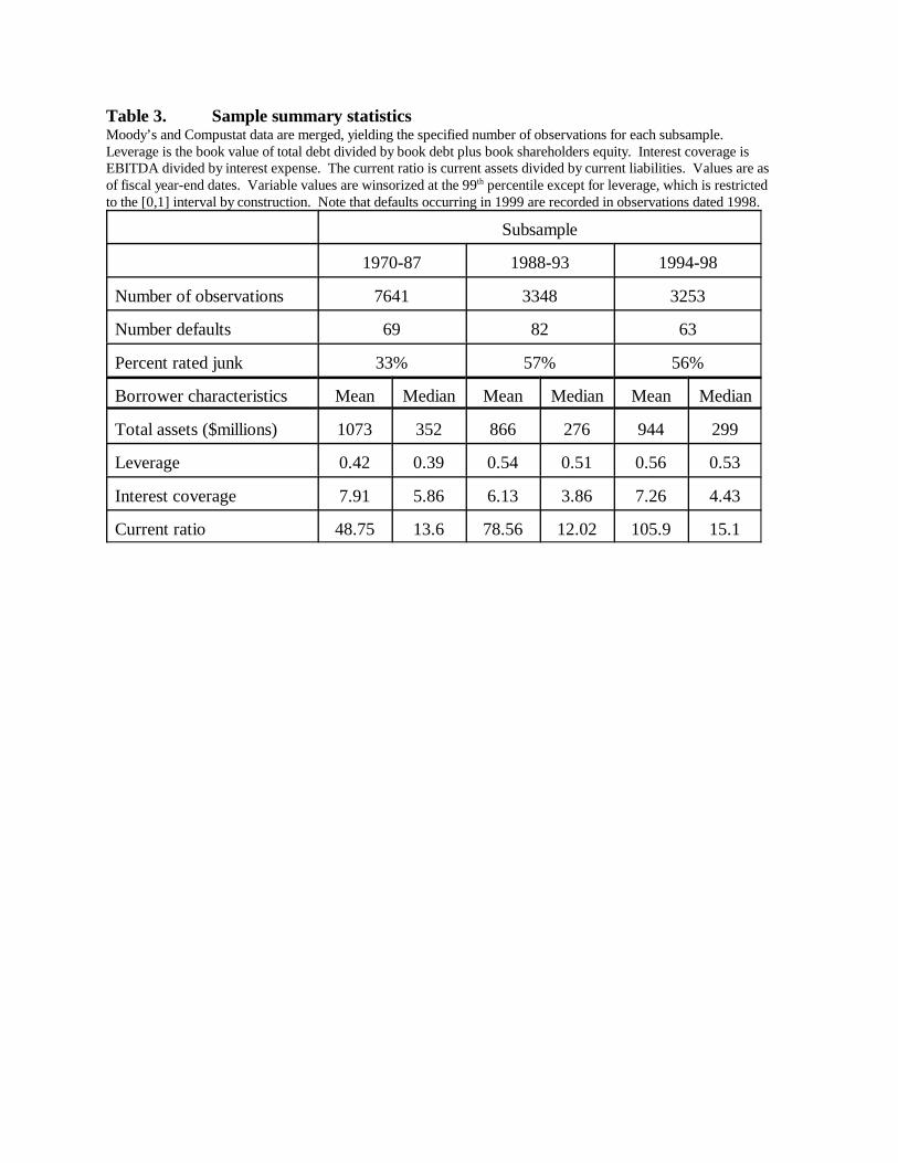
Table 3. Sample summary statisticsMoody’s and Compustat data are merged, yielding the specified number of observations for each subsample. Leverage is the book value of total debt divided by book debt plus book shareholders equity. Interest coverage isEBITDA divided by interest expense. The current ratio is current assets divided by current liabilities. Values are asof fiscal year-end dates. Variable values are winsorized at the 99th percentile except for leverage, which is restrictedto the [0,1] interval by construction. Note that defaults occurring in 1999 are recorded in observations dated 1998.
Subsample
1970-87 1988-93 1994-98
Number of observations 7641 3348 3253
Number defaults 69 82 63
Percent rated junk 33% 57% 56%
Borrower characteristics Mean Median Mean Median Mean Median
Total assets ($millions) 1073 352 866 276 944 299
Leverage 0.42 0.39 0.54 0.51 0.56 0.53
Interest coverage 7.91 5.86 6.13 3.86 7.26 4.43
Current ratio 48.75 13.6 78.56 12.02 105.9 15.1
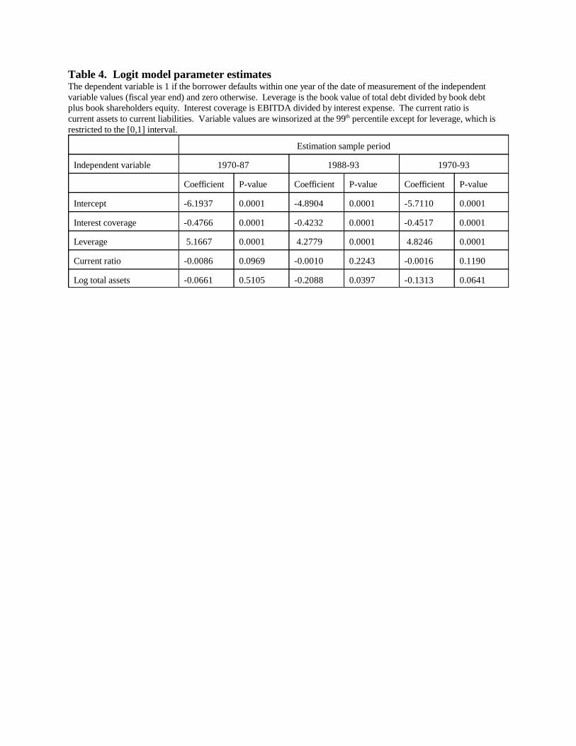
Table 4. Logit model parameter estimatesThe dependent variable is 1 if the borrower defaults within one year of the date of measurement of the independentvariable values (fiscal year end) and zero otherwise. Leverage is the book value of total debt divided by book debtplus book shareholders equity. Interest coverage is EBITDA divided by interest expense. The current ratio iscurrent assets to current liabilities. Variable values are winsorized at the 99th percentile except for leverage, which isrestricted to the [0,1] interval.
Estimation sample period
Independent variable 1970-87 1988-93 1970-93
Coefficient P-value Coefficient P-value Coefficient P-value
Intercept -6.1937 0.0001 -4.8904 0.0001 -5.7110 0.0001
Interest coverage -0.4766 0.0001 -0.4232 0.0001 -0.4517 0.0001
Leverage 5.1667 0.0001 4.2779 0.0001 4.8246 0.0001
Current ratio -0.0086 0.0969 -0.0010 0.2243 -0.0016 0.1190
Log total assets -0.0661 0.5105 -0.2088 0.0397 -0.1313 0.0641
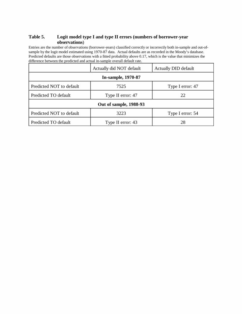
Table 5. Logit model type I and type II errors (numbers of borrower-yearobservations)
Entries are the number of observations (borrower-years) classified correctly or incorrectly both in-sample and out-of-sample by the logit model estimated using 1970-87 data. Actual defaults are as recorded in the Moody’s database. Predicted defaults are those observations with a fitted probability above 0.17, which is the value that minimizes thedifference between the predicted and actual in-sample overall default rate.
Actually did NOT default Actually DID default
In-sample, 1970-87
Predicted NOT to default 7525 Type I error: 47
Predicted TO default Type II error: 47 22
Out of sample, 1988-93
Predicted NOT to default 3223 Type I error: 54
Predicted TO default Type II error: 43 28

Table 6. Default probability ranges for two simulated rating scales.Observations (borrower-years) are assigned to the simulated grade on each scale for which the specified rangebrackets the observation’s logit model fitted default probability value.
Borrowers with fitted probability values inthis range...
Are assigned this simulated grade
Scale5
< 0.001 1
0.001 to 0.0025 2
0.0025 to 0.01 3
0.01 to 0.05 4
>= 0.05 5
Scale10
< 0.001 a
0.001 to 0.002 b
0.002 to 0.004 c
0.004 to 0.008 d
0.008 to 0.0125 e
0.0125 to 0.02 f
0.02 to 0.03 g
0.03 to 0.05 h
0.05 to 0.10 i
>= 0.10 j
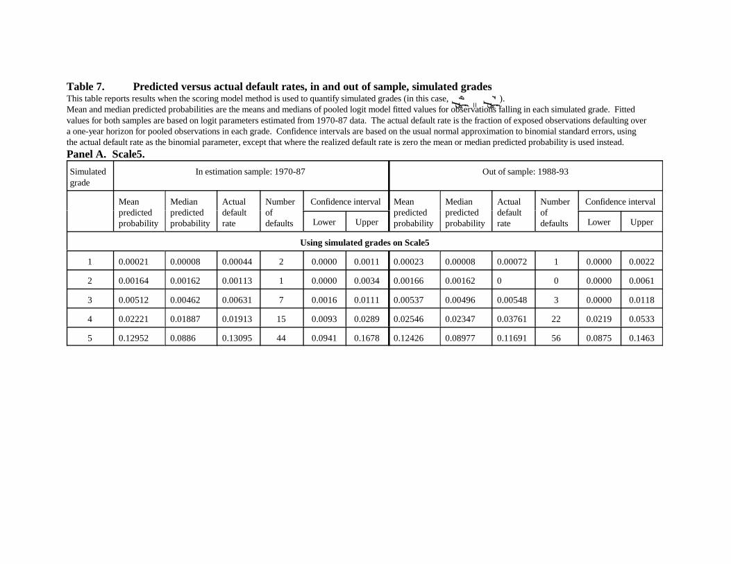
Table 7. Predicted versus actual default rates, in and out of sample, simulated gradesThis table reports results when the scoring model method is used to quantify simulated grades (in this case, ). Mean and median predicted probabilities are the means and medians of pooled logit model fitted values for observations falling in each simulated grade. Fittedvalues for both samples are based on logit parameters estimated from 1970-87 data. The actual default rate is the fraction of exposed observations defaulting overa one-year horizon for pooled observations in each grade. Confidence intervals are based on the usual normal approximation to binomial standard errors, usingthe actual default rate as the binomial parameter, except that where the realized default rate is zero the mean or median predicted probability is used instead.Panel A. Scale5.
Simulatedgrade
In estimation sample: 1970-87 Out of sample: 1988-93
Meanpredictedprobability
Medianpredictedprobability
Actualdefaultrate
Numberofdefaults
Confidence interval Meanpredictedprobability
Medianpredictedprobability
Actualdefaultrate
Numberofdefaults
Confidence interval
Lower Upper Lower Upper
Using simulated grades on Scale5
1 0.00021 0.00008 0.00044 2 0.0000 0.0011 0.00023 0.00008 0.00072 1 0.0000 0.0022
2 0.00164 0.00162 0.00113 1 0.0000 0.0034 0.00166 0.00162 0 0 0.0000 0.0061
3 0.00512 0.00462 0.00631 7 0.0016 0.0111 0.00537 0.00496 0.00548 3 0.0000 0.0118
4 0.02221 0.01887 0.01913 15 0.0093 0.0289 0.02546 0.02347 0.03761 22 0.0219 0.0533
5 0.12952 0.0886 0.13095 44 0.0941 0.1678 0.12426 0.08977 0.11691 56 0.0875 0.1463
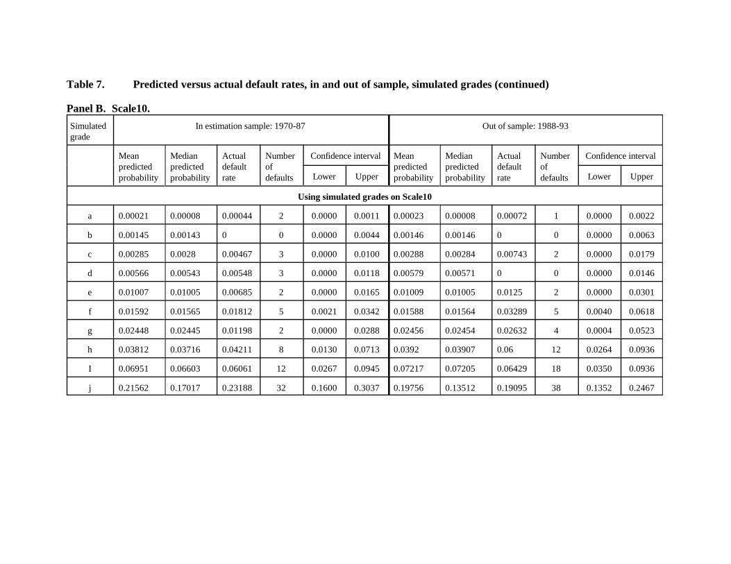
Table 7. Predicted versus actual default rates, in and out of sample, simulated grades (continued)
Panel B. Scale10.
Simulatedgrade
In estimation sample: 1970-87 Out of sample: 1988-93
Meanpredictedprobability
Medianpredictedprobability
Actualdefaultrate
Numberofdefaults
Confidence interval Meanpredictedprobability
Medianpredictedprobability
Actualdefaultrate
Numberofdefaults
Confidence interval
Lower Upper Lower Upper
Using simulated grades on Scale10
a 0.00021 0.00008 0.00044 2 0.0000 0.0011 0.00023 0.00008 0.00072 1 0.0000 0.0022
b 0.00145 0.00143 0 0 0.0000 0.0044 0.00146 0.00146 0 0 0.0000 0.0063
c 0.00285 0.0028 0.00467 3 0.0000 0.0100 0.00288 0.00284 0.00743 2 0.0000 0.0179
d 0.00566 0.00543 0.00548 3 0.0000 0.0118 0.00579 0.00571 0 0 0.0000 0.0146
e 0.01007 0.01005 0.00685 2 0.0000 0.0165 0.01009 0.01005 0.0125 2 0.0000 0.0301
f 0.01592 0.01565 0.01812 5 0.0021 0.0342 0.01588 0.01564 0.03289 5 0.0040 0.0618
g 0.02448 0.02445 0.01198 2 0.0000 0.0288 0.02456 0.02454 0.02632 4 0.0004 0.0523
h 0.03812 0.03716 0.04211 8 0.0130 0.0713 0.0392 0.03907 0.06 12 0.0264 0.0936
I 0.06951 0.06603 0.06061 12 0.0267 0.0945 0.07217 0.07205 0.06429 18 0.0350 0.0936
j 0.21562 0.17017 0.23188 32 0.1600 0.3037 0.19756 0.13512 0.19095 38 0.1352 0.2467
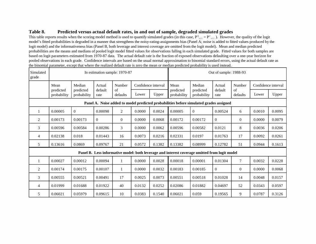
Table 8. Predicted versus actual default rates, in and out of sample, degraded simulated gradesThis table reports results when the scoring model method is used to quantify simulated grades (in this case, Pqnit = Prnit ). However, the quality of the logitmodel’s fitted probabilities is degraded in a manner that strengthens the noisy-rating-assignments bias (Panel A; noise is added to fitted values produced by thelogit model) and the informativeness bias (Panel B, both leverage and interest coverage are omitted from the logit model). Mean and median predictedprobabilities are the means and medians of pooled logit model fitted values for observations falling in each simulated grade. Fitted values for both samples arebased on logit parameters estimated from 1970-87 data. The actual default rate is the fraction of exposed observations defaulting over a one-year horizon forpooled observations in each grade. Confidence intervals are based on the usual normal approximation to binomial standard errors, using the actual default rate asthe binomial parameter, except that where the realized default rate is zero the mean or median predicted probability is used instead.
Simulatedgrade
In estimation sample: 1970-87 Out of sample: 1988-93
Meanpredictedprobability
Medianpredictedprobability
Actualdefaultrate
Numberofdefaults
Confidence interval Meanpredictedprobability
Medianpredictedprobability
Actualdefaultrate
Numberofdefaults
Confidence interval
Lower Upper Lower Upper
Panel A. Noise added to model predicted probabilities before simulated grades assigned
1 0.00005 0 0.00098 2 0.0000 0.0024 0.00005 0 0.00524 6 0.0010 0.0095
2 0.00173 0.00173 0 0 0.0000 0.0068 0.00172 0.00172 0 0 0.0000 0.0079
3 0.00596 0.00584 0.00286 3 0.0000 0.0062 0.00596 0.00582 0.0121 8 0.0036 0.0206
4 0.02138 0.018 0.01443 16 0.0073 0.0216 0.02331 0.0197 0.01763 17 0.0092 0.0261
5 0.13616 0.0869 0.09767 21 0.0572 0.1382 0.13382 0.08999 0.12782 51 0.0944 0.1613
Panel B. Less informative model: both leverage and interest coverage omitted from logit model
1 0.00027 0.00012 0.00094 1 0.0000 0.0028 0.00018 0.00001 0.01304 7 0.0032 0.0228
2 0.00174 0.00175 0.00107 1 0.0000 0.0032 0.00183 0.00185 0 0 0.0000 0.0068
3 0.00555 0.00521 0.00491 17 0.0025 0.0073 0.00551 0.00518 0.01028 14 0.0048 0.0157
4 0.01999 0.01688 0.01922 40 0.0132 0.0252 0.02086 0.01882 0.04697 52 0.0343 0.0597
5 0.06021 0.05979 0.09615 10 0.0383 0.1540 0.06021 0.059 0.19565 9 0.0787 0.3126
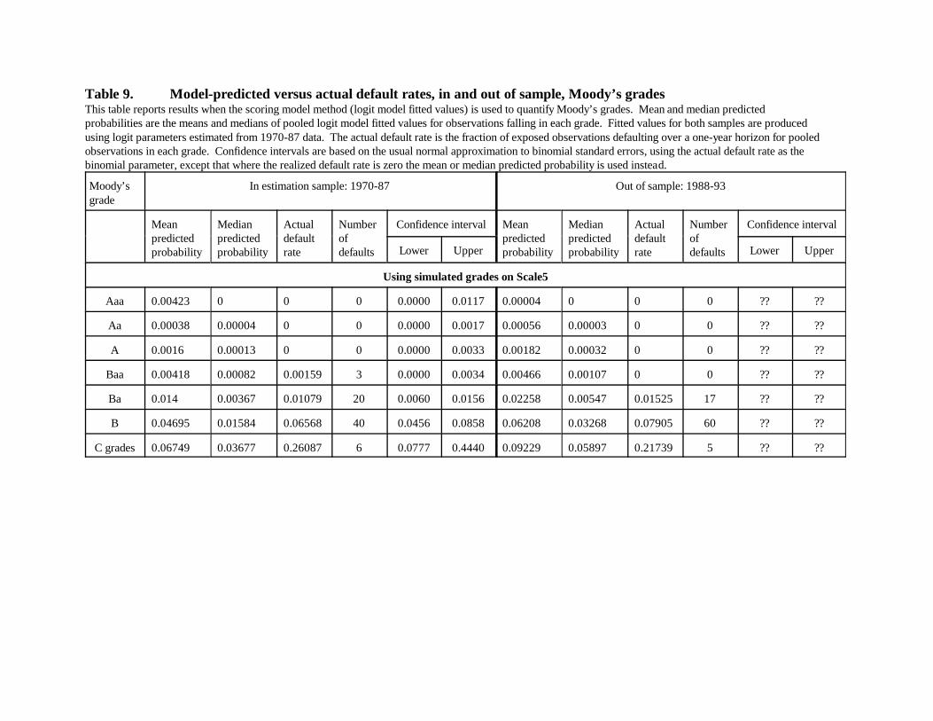
Table 9. Model-predicted versus actual default rates, in and out of sample, Moody’s gradesThis table reports results when the scoring model method (logit model fitted values) is used to quantify Moody’s grades. Mean and median predictedprobabilities are the means and medians of pooled logit model fitted values for observations falling in each grade. Fitted values for both samples are producedusing logit parameters estimated from 1970-87 data. The actual default rate is the fraction of exposed observations defaulting over a one-year horizon for pooledobservations in each grade. Confidence intervals are based on the usual normal approximation to binomial standard errors, using the actual default rate as thebinomial parameter, except that where the realized default rate is zero the mean or median predicted probability is used instead.
Moody’sgrade
In estimation sample: 1970-87 Out of sample: 1988-93
Meanpredictedprobability
Medianpredictedprobability
Actualdefaultrate
Numberofdefaults
Confidence interval Meanpredictedprobability
Medianpredictedprobability
Actualdefaultrate
Numberofdefaults
Confidence interval
Lower Upper Lower Upper
Using simulated grades on Scale5
Aaa 0.00423 0 0 0 0.0000 0.0117 0.00004 0 0 0 ?? ??
Aa 0.00038 0.00004 0 0 0.0000 0.0017 0.00056 0.00003 0 0 ?? ??
A 0.0016 0.00013 0 0 0.0000 0.0033 0.00182 0.00032 0 0 ?? ??
Baa 0.00418 0.00082 0.00159 3 0.0000 0.0034 0.00466 0.00107 0 0 ?? ??
Ba 0.014 0.00367 0.01079 20 0.0060 0.0156 0.02258 0.00547 0.01525 17 ?? ??
B 0.04695 0.01584 0.06568 40 0.0456 0.0858 0.06208 0.03268 0.07905 60 ?? ??
C grades 0.06749 0.03677 0.26087 6 0.0777 0.4440 0.09229 0.05897 0.21739 5 ?? ??
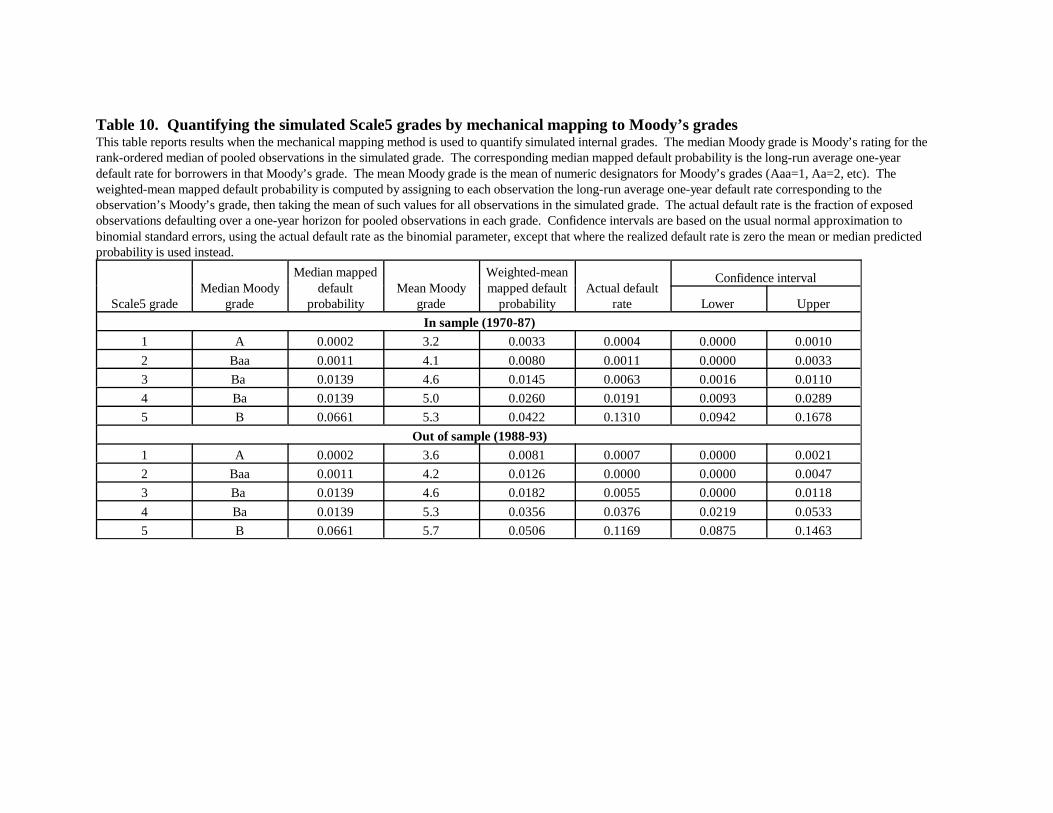
Table 10. Quantifying the simulated Scale5 grades by mechanical mapping to Moody’s gradesThis table reports results when the mechanical mapping method is used to quantify simulated internal grades. The median Moody grade is Moody’s rating for therank-ordered median of pooled observations in the simulated grade. The corresponding median mapped default probability is the long-run average one-yeardefault rate for borrowers in that Moody’s grade. The mean Moody grade is the mean of numeric designators for Moody’s grades (Aaa=1, Aa=2, etc). Theweighted-mean mapped default probability is computed by assigning to each observation the long-run average one-year default rate corresponding to theobservation’s Moody’s grade, then taking the mean of such values for all observations in the simulated grade. The actual default rate is the fraction of exposedobservations defaulting over a one-year horizon for pooled observations in each grade. Confidence intervals are based on the usual normal approximation tobinomial standard errors, using the actual default rate as the binomial parameter, except that where the realized default rate is zero the mean or median predictedprobability is used instead.
Scale5 gradeMedian Moody
grade
Median mappeddefault
probabilityMean Moody
grade
Weighted-meanmapped default
probabilityActual default
rate
Confidence interval
Lower Upper
In sample (1970-87)1 A 0.0002 3.2 0.0033 0.0004 0.0000 0.0010
2 Baa 0.0011 4.1 0.0080 0.0011 0.0000 0.0033
3 Ba 0.0139 4.6 0.0145 0.0063 0.0016 0.0110
4 Ba 0.0139 5.0 0.0260 0.0191 0.0093 0.0289
5 B 0.0661 5.3 0.0422 0.1310 0.0942 0.1678
Out of sample (1988-93)1 A 0.0002 3.6 0.0081 0.0007 0.0000 0.0021
2 Baa 0.0011 4.2 0.0126 0.0000 0.0000 0.0047
3 Ba 0.0139 4.6 0.0182 0.0055 0.0000 0.0118
4 Ba 0.0139 5.3 0.0356 0.0376 0.0219 0.0533
5 B 0.0661 5.7 0.0506 0.1169 0.0875 0.1463
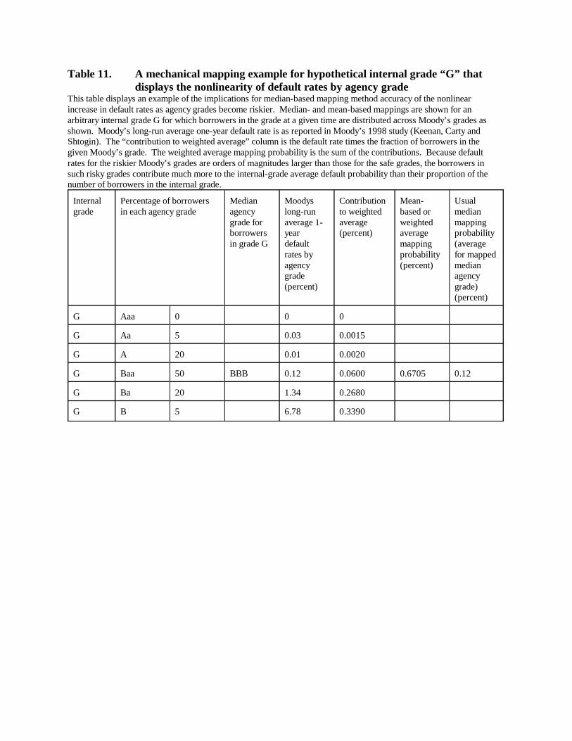
Table 11. A mechanical mapping example for hypothetical internal grade “G” thatdisplays the nonlinearity of default rates by agency grade
This table displays an example of the implications for median-based mapping method accuracy of the nonlinearincrease in default rates as agency grades become riskier. Median- and mean-based mappings are shown for anarbitrary internal grade G for which borrowers in the grade at a given time are distributed across Moody’s grades asshown. Moody’s long-run average one-year default rate is as reported in Moody’s 1998 study (Keenan, Carty andShtogin). The “contribution to weighted average” column is the default rate times the fraction of borrowers in thegiven Moody’s grade. The weighted average mapping probability is the sum of the contributions. Because defaultrates for the riskier Moody’s grades are orders of magnitudes larger than those for the safe grades, the borrowers insuch risky grades contribute much more to the internal-grade average default probability than their proportion of thenumber of borrowers in the internal grade.
Internalgrade
Percentage of borrowersin each agency grade
Medianagencygrade forborrowersin grade G
Moodyslong-runaverage 1-yeardefaultrates byagencygrade(percent)
Contributionto weightedaverage(percent)
Mean-based orweightedaveragemappingprobability(percent)
Usualmedianmappingprobability(averagefor mappedmedianagencygrade)(percent)
G Aaa 0 0 0
G Aa 5 0.03 0.0015
G A 20 0.01 0.0020
G Baa 50 BBB 0.12 0.0600 0.6705 0.12
G Ba 20 1.34 0.2680
G B 5 6.78 0.3390
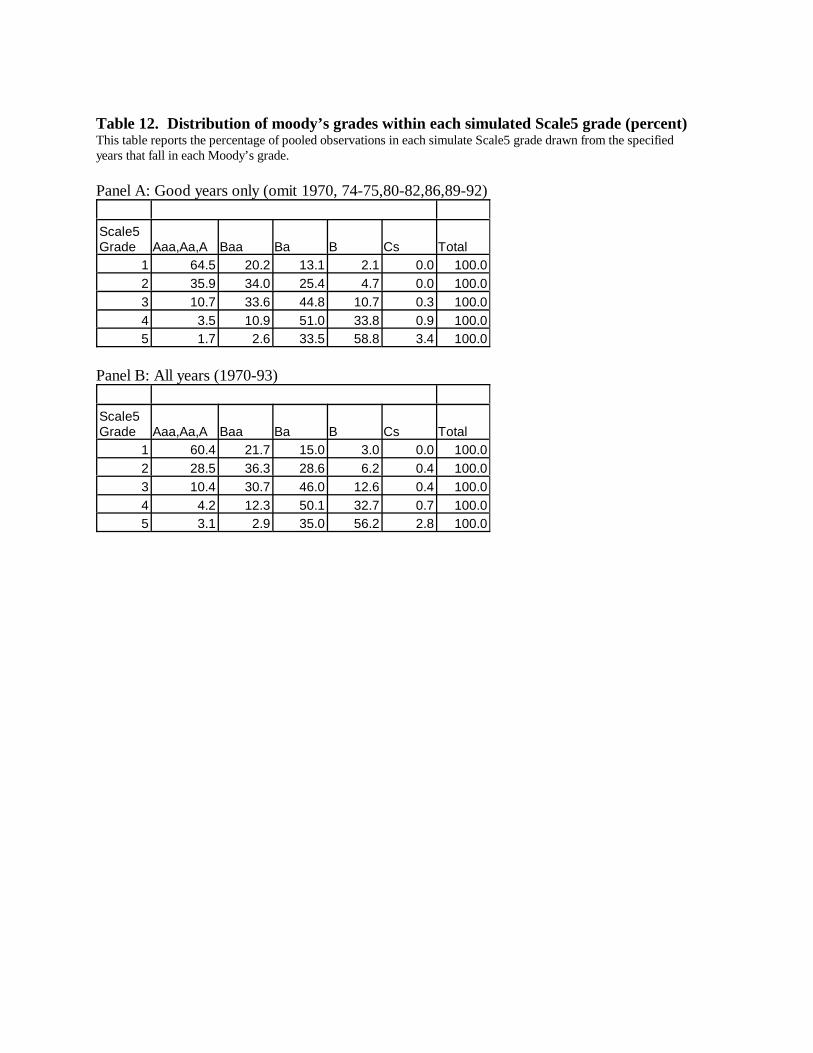
Table 12. Distribution of moody’s grades within each simulated Scale5 grade (percent)This table reports the percentage of pooled observations in each simulate Scale5 grade drawn from the specifiedyears that fall in each Moody’s grade.
Panel A: Good years only (omit 1970, 74-75,80-82,86,89-92)
Scale5Grade Aaa,Aa,A Baa Ba B Cs Total
1 64.5 20.2 13.1 2.1 0.0 100.02 35.9 34.0 25.4 4.7 0.0 100.03 10.7 33.6 44.8 10.7 0.3 100.04 3.5 10.9 51.0 33.8 0.9 100.05 1.7 2.6 33.5 58.8 3.4 100.0
Panel B: All years (1970-93)
Scale5Grade Aaa,Aa,A Baa Ba B Cs Total
1 60.4 21.7 15.0 3.0 0.0 100.02 28.5 36.3 28.6 6.2 0.4 100.03 10.4 30.7 46.0 12.6 0.4 100.04 4.2 12.3 50.1 32.7 0.7 100.05 3.1 2.9 35.0 56.2 2.8 100.0
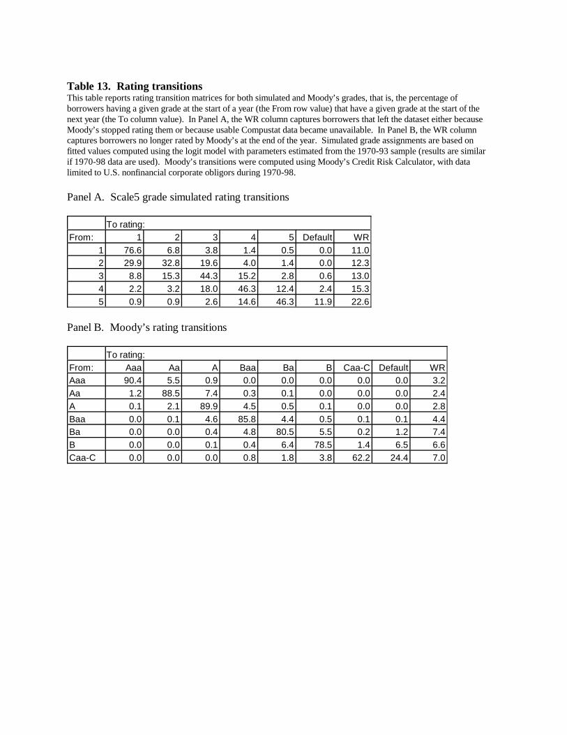
Table 13. Rating transitionsThis table reports rating transition matrices for both simulated and Moody’s grades, that is, the percentage ofborrowers having a given grade at the start of a year (the From row value) that have a given grade at the start of thenext year (the To column value). In Panel A, the WR column captures borrowers that left the dataset either becauseMoody’s stopped rating them or because usable Compustat data became unavailable. In Panel B, the WR columncaptures borrowers no longer rated by Moody’s at the end of the year. Simulated grade assignments are based onfitted values computed using the logit model with parameters estimated from the 1970-93 sample (results are similarif 1970-98 data are used). Moody’s transitions were computed using Moody’s Credit Risk Calculator, with datalimited to U.S. nonfinancial corporate obligors during 1970-98.
Panel A. Scale5 grade simulated rating transitions
To rating:From: 1 2 3 4 5 Default WR
1 76.6 6.8 3.8 1.4 0.5 0.0 11.02 29.9 32.8 19.6 4.0 1.4 0.0 12.33 8.8 15.3 44.3 15.2 2.8 0.6 13.04 2.2 3.2 18.0 46.3 12.4 2.4 15.35 0.9 0.9 2.6 14.6 46.3 11.9 22.6
Panel B. Moody’s rating transitions
To rating:From: Aaa Aa A Baa Ba B Caa-C Default WRAaa 90.4 5.5 0.9 0.0 0.0 0.0 0.0 0.0 3.2Aa 1.2 88.5 7.4 0.3 0.1 0.0 0.0 0.0 2.4A 0.1 2.1 89.9 4.5 0.5 0.1 0.0 0.0 2.8Baa 0.0 0.1 4.6 85.8 4.4 0.5 0.1 0.1 4.4Ba 0.0 0.0 0.4 4.8 80.5 5.5 0.2 1.2 7.4B 0.0 0.0 0.1 0.4 6.4 78.5 1.4 6.5 6.6Caa-C 0.0 0.0 0.0 0.8 1.8 3.8 62.2 24.4 7.0
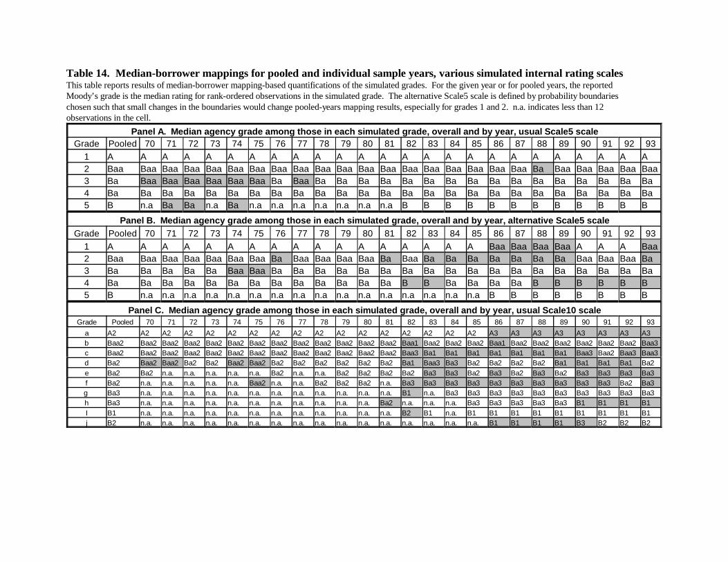
Table 14. Median-borrower mappings for pooled and individual sample years, various simulated internal rating scalesThis table reports results of median-borrower mapping-based quantifications of the simulated grades. For the given year or for pooled years, the reportedMoody’s grade is the median rating for rank-ordered observations in the simulated grade. The alternative Scale5 scale is defined by probability boundarieschosen such that small changes in the boundaries would change pooled-years mapping results, especially for grades 1 and 2. n.a. indicates less than 12observations in the cell.
Panel A. Median agency grade among those in each simulated grade, overall and by year, usual Scale5 scaleGrade Pooled 70 71 72 73 74 75 76 77 78 79 80 81 82 83 84 85 86 87 88 89 90 91 92 93
1 A A A A A A A A A A A A A A A A A A A A A A A A A2 Baa Baa Baa Baa Baa Baa Baa Baa Baa Baa Baa Baa Baa Baa Baa Baa Baa Baa Baa Ba Baa Baa Baa Baa Baa3 Ba Baa Baa Baa Baa Baa Baa Ba Baa Ba Ba Ba Ba Ba Ba Ba Ba Ba Ba Ba Ba Ba Ba Ba Ba4 Ba Ba Ba Ba Ba Ba Ba Ba Ba Ba Ba Ba Ba Ba Ba Ba Ba Ba Ba Ba Ba Ba Ba Ba Ba5 B n.a Ba Ba n.a Ba n.a n.a n.a n.a n.a n.a n.a B B B B B B B B B B B B
Panel B. Median agency grade among those in each simulated grade, overall and by year, alternative Scale5 scaleGrade Pooled 70 71 72 73 74 75 76 77 78 79 80 81 82 83 84 85 86 87 88 89 90 91 92 93
1 A A A A A A A A A A A A A A A A A Baa Baa Baa Baa A A A Baa2 Baa Baa Baa Baa Baa Baa Baa Ba Baa Baa Baa Baa Ba Baa Ba Ba Ba Ba Ba Ba Ba Baa Baa Baa Ba3 Ba Ba Ba Ba Ba Baa Baa Ba Ba Ba Ba Ba Ba Ba Ba Ba Ba Ba Ba Ba Ba Ba Ba Ba Ba4 Ba Ba Ba Ba Ba Ba Ba Ba Ba Ba Ba Ba Ba B B Ba Ba Ba Ba B B B B B B5 B n.a n.a n.a n.a n.a n.a n.a n.a n.a n.a n.a n.a n.a n.a n.a n.a B B B B B B B B
Panel C. Median agency grade among those in each simulated grade, overall and by year, usual Scale10 scaleGrade Pooled 70 71 72 73 74 75 76 77 78 79 80 81 82 83 84 85 86 87 88 89 90 91 92 93
a A2 A2 A2 A2 A2 A2 A2 A2 A2 A2 A2 A2 A2 A2 A2 A2 A2 A3 A3 A3 A3 A3 A3 A3 A3b Baa2 Baa2 Baa2 Baa2 Baa2 Baa2 Baa2 Baa2 Baa2 Baa2 Baa2 Baa2 Baa2 Baa1 Baa2 Baa2 Baa2 Baa1 Baa2 Baa2 Baa2 Baa2 Baa2 Baa2 Baa3c Baa2 Baa2 Baa2 Baa2 Baa2 Baa2 Baa2 Baa2 Baa2 Baa2 Baa2 Baa2 Baa2 Baa3 Ba1 Ba1 Ba1 Ba1 Ba1 Ba1 Ba1 Baa3 Baa2 Baa3 Baa3d Ba2 Baa2 Baa2 Ba2 Ba2 Baa2 Baa2 Ba2 Ba2 Ba2 Ba2 Ba2 Ba2 Ba1 Baa3 Ba3 Ba2 Ba2 Ba2 Ba2 Ba1 Ba1 Ba1 Ba1 Ba2e Ba2 Ba2 n.a. n.a. n.a. n.a. n.a. Ba2 n.a. n.a. Ba2 Ba2 Ba2 Ba2 Ba3 Ba3 Ba2 Ba3 Ba2 Ba3 Ba2 Ba3 Ba3 Ba3 Ba3f Ba2 n.a. n.a. n.a. n.a. n.a. Baa2 n.a. n.a. Ba2 Ba2 Ba2 n.a. Ba3 Ba3 Ba3 Ba3 Ba3 Ba3 Ba3 Ba3 Ba3 Ba3 Ba2 Ba3g Ba3 n.a. n.a. n.a. n.a. n.a. n.a. n.a. n.a. n.a. n.a. n.a. n.a. B1 n.a. Ba3 Ba3 Ba3 Ba3 Ba3 Ba3 Ba3 Ba3 Ba3 Ba3h Ba3 n.a. n.a. n.a. n.a. n.a. n.a. n.a. n.a. n.a. n.a. n.a. Ba2 n.a. n.a. n.a. Ba3 Ba3 Ba3 Ba3 Ba3 B1 B1 B1 B1I B1 n.a. n.a. n.a. n.a. n.a. n.a. n.a. n.a. n.a. n.a. n.a. n.a. B2 B1 n.a. B1 B1 B1 B1 B1 B1 B1 B1 B1j B2 n.a. n.a. n.a. n.a. n.a. n.a. n.a. n.a. n.a. n.a. n.a. n.a. n.a. n.a. n.a. n.a. B1 B1 B1 B1 B3 B2 B2 B2
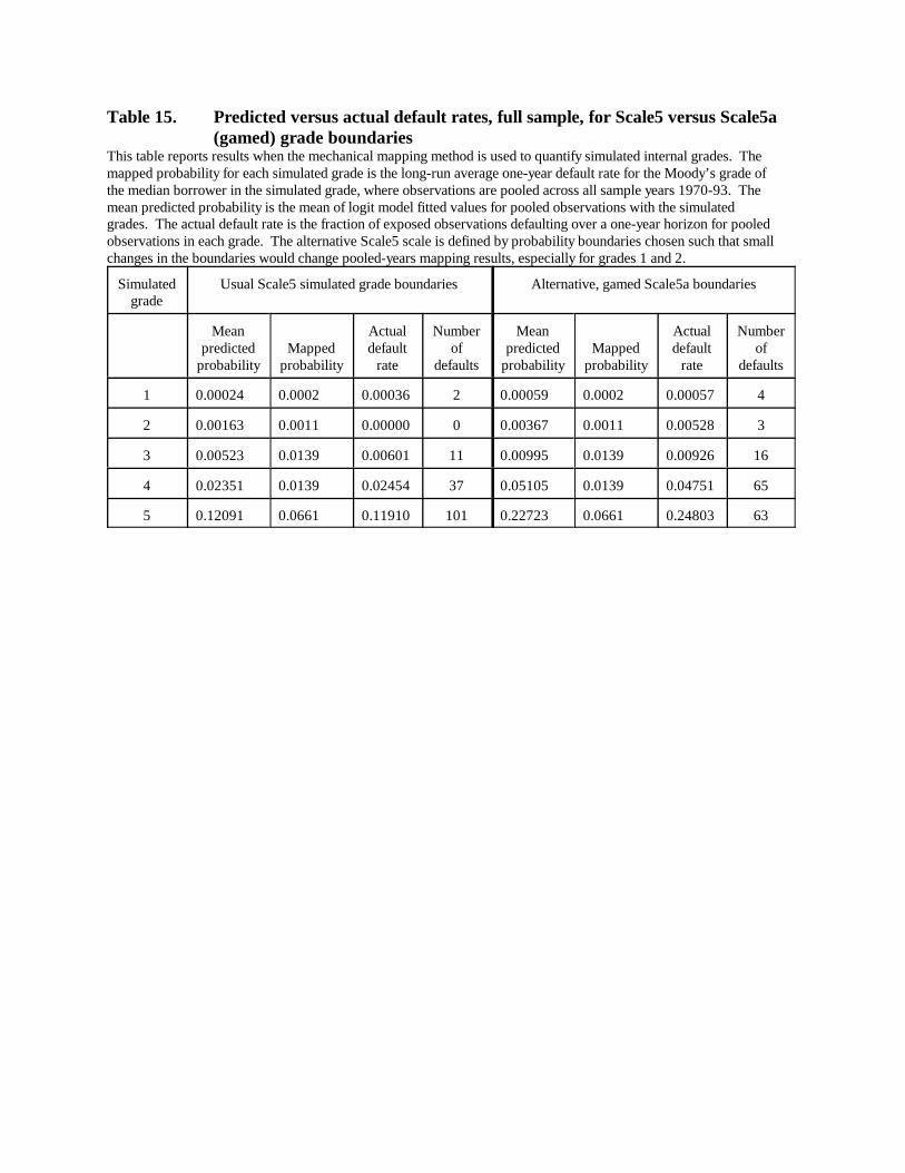
Table 15. Predicted versus actual default rates, full sample, for Scale5 versus Scale5a(gamed) grade boundaries
This table reports results when the mechanical mapping method is used to quantify simulated internal grades. Themapped probability for each simulated grade is the long-run average one-year default rate for the Moody’s grade ofthe median borrower in the simulated grade, where observations are pooled across all sample years 1970-93. Themean predicted probability is the mean of logit model fitted values for pooled observations with the simulatedgrades. The actual default rate is the fraction of exposed observations defaulting over a one-year horizon for pooledobservations in each grade. The alternative Scale5 scale is defined by probability boundaries chosen such that smallchanges in the boundaries would change pooled-years mapping results, especially for grades 1 and 2.
Simulatedgrade
Usual Scale5 simulated grade boundaries Alternative, gamed Scale5a boundaries
Meanpredicted
probabilityMapped
probability
Actualdefault
rate
Numberof
defaults
Meanpredicted
probabilityMapped
probability
Actualdefault
rate
Numberof
defaults
1 0.00024 0.0002 0.00036 2 0.00059 0.0002 0.00057 4
2 0.00163 0.0011 0.00000 0 0.00367 0.0011 0.00528 3
3 0.00523 0.0139 0.00601 11 0.00995 0.0139 0.00926 16
4 0.02351 0.0139 0.02454 37 0.05105 0.0139 0.04751 65
5 0.12091 0.0661 0.11910 101 0.22723 0.0661 0.24803 63

Table 16. Effects of gaming of scoring model by directing portfolio investment toborrowers about which the model is too optimistic
This table reports actual default rates for two pooled sets of simulated portfolios. In the base case, we construct 100simulated debt portfolios, each with 250 assets, by drawing randomly 50 observations from the pool of allobservations assigned each simulated Scale5 grade. In the gamed case, we again draw from assets assigned eachsimulated Scale5 grade, but draws are limited to observations with fitted values from an expanded logit model thatare higher than corresponding base logit model fitted values. The expanded logit model includes dummies for theborrower’s Moody’s rating. Thus, the expanded model’s fitted values carry more information and relatively largefitted values are more likely to designate relatively risky assets.
Simulated Grade
Actual Default Rate forBase, Ungamed
Portfolio
Actual Default Rate forGamed Portfolio
(Information in AgencyRatings Exploited)
1 0.0002 0.00182 0.0000 0.00003 0.0062 0.01324 0.0220 0.04405 0.1120 0.1412
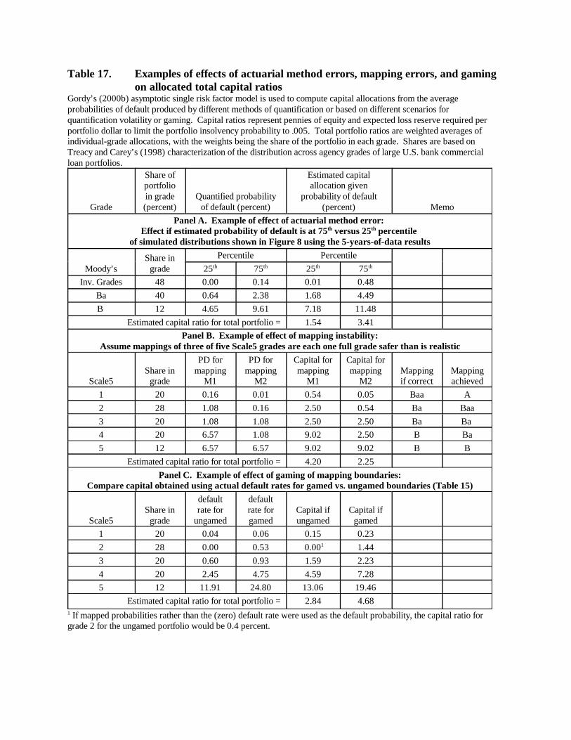
Table 17. Examples of effects of actuarial method errors, mapping errors, and gamingon allocated total capital ratios
Gordy’s (2000b) asymptotic single risk factor model is used to compute capital allocations from the averageprobabilities of default produced by different methods of quantification or based on different scenarios forquantification volatility or gaming. Capital ratios represent pennies of equity and expected loss reserve required perportfolio dollar to limit the portfolio insolvency probability to .005. Total portfolio ratios are weighted averages ofindividual-grade allocations, with the weights being the share of the portfolio in each grade. Shares are based onTreacy and Carey’s (1998) characterization of the distribution across agency grades of large U.S. bank commercialloan portfolios.
Grade
Share ofportfolioin grade(percent)
Quantified probabilityof default (percent)
Estimated capitalallocation given
probability of default(percent) Memo
Panel A. Example of effect of actuarial method error: Effect if estimated probability of default is at 75th versus 25th percentile
of simulated distributions shown in Figure 8 using the 5-years-of-data results
Moody’sShare ingrade
Percentile Percentile
25th 75th 25th 75th
Inv. Grades 48 0.00 0.14 0.01 0.48
Ba 40 0.64 2.38 1.68 4.49
B 12 4.65 9.61 7.18 11.48
Estimated capital ratio for total portfolio = 1.54 3.41
Panel B. Example of effect of mapping instability:Assume mappings of three of five Scale5 grades are each one full grade safer than is realistic
Scale5Share ingrade
PD formapping
M1
PD formapping
M2
Capital formapping
M1
Capital formapping
M2Mappingif correct
Mappingachieved
1 20 0.16 0.01 0.54 0.05 Baa A
2 28 1.08 0.16 2.50 0.54 Ba Baa
3 20 1.08 1.08 2.50 2.50 Ba Ba
4 20 6.57 1.08 9.02 2.50 B Ba
5 12 6.57 6.57 9.02 9.02 B B
Estimated capital ratio for total portfolio = 4.20 2.25
Panel C. Example of effect of gaming of mapping boundaries:Compare capital obtained using actual default rates for gamed vs. ungamed boundaries (Table 15)
Scale5Share ingrade
defaultrate for
ungamed
defaultrate forgamed
Capital ifungamed
Capital ifgamed
1 20 0.04 0.06 0.15 0.23
2 28 0.00 0.53 0.001 1.44
3 20 0.60 0.93 1.59 2.23
4 20 2.45 4.75 4.59 7.28
5 12 11.91 24.80 13.06 19.46
Estimated capital ratio for total portfolio = 2.84 4.681 If mapped probabilities rather than the (zero) default rate were used as the default probability, the capital ratio forgrade 2 for the ungamed portfolio would be 0.4 percent.
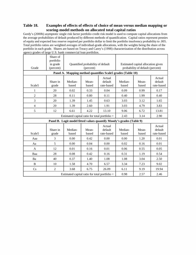
Table 18. Examples of effects of effects of choice of mean versus median mapping orscoring-model methods on allocated total capital ratios
Gordy’s (2000b) asymptotic single risk factor portfolio credit risk model is used to compute capital allocations fromthe average probabilities of default produced by different methods of quantification. Capital ratios represent penniesof equity and expected loss reserve required per portfolio dollar to limit the portfolio insolvency probability to .005. Total portfolio ratios are weighted averages of individual-grade allocations, with the weights being the share of theportfolio in each grade. Shares are based on Treacy and Carey’s (1998) characterization of the distribution acrossagency grades of large U.S. bank commercial loan portfolios.
Grade
Share ofportfolioin grade(percent)
Quantified probability of default(percent)
Estimated capital allocation givenprobability of default (percent)
Panel A. Mapping method quantifies Scale5 grades (Table 10)
Scale5Share ingrade
Median-based
Mean-based
Actualdefault
rate-basedMedian-based
Mean-based
Actualdefault
rate-based
1 20 0.02 0.33 0.04 0.09 0.99 0.17
2 28 0.11 0.80 0.11 0.40 1.99 0.40
3 20 1.39 1.45 0.63 3.03 3.12 1.65
4 20 1.39 2.60 1.91 3.03 4.79 3.83
5 12 6.61 4.22 13.10 9.06 6.72 13.81
Estimated capital ratio for total portfolio = 2.43 3.14 2.90
Panel B. Logit model fitted values quantify Moody’s grades (Table 9)
Scale5Share in
gradeMedian-
basedMean-based
Actualdefault
rate-basedMedian-
basedMean-based
Actualdefault
rate-based
Aaa 3 0.00 0.42 0.00 0.00 1.20 0.01
Aa 5 0.00 0.04 0.00 0.02 0.16 0.01
A 12 0.01 0.16 0.01 0.06 0.55 0.05
Baa 28 0.08 0.42 0.16 0.31 1.19 0.54
Ba 40 0.37 1.40 1.08 1.08 3.04 2.50
B 10 1.58 4.70 6.57 3.34 7.23 9.02
Cs 2 3.68 6.75 26.09 6.11 9.19 19.94
Estimated capital ratio for total portfolio = 0.98 2.57 2.46
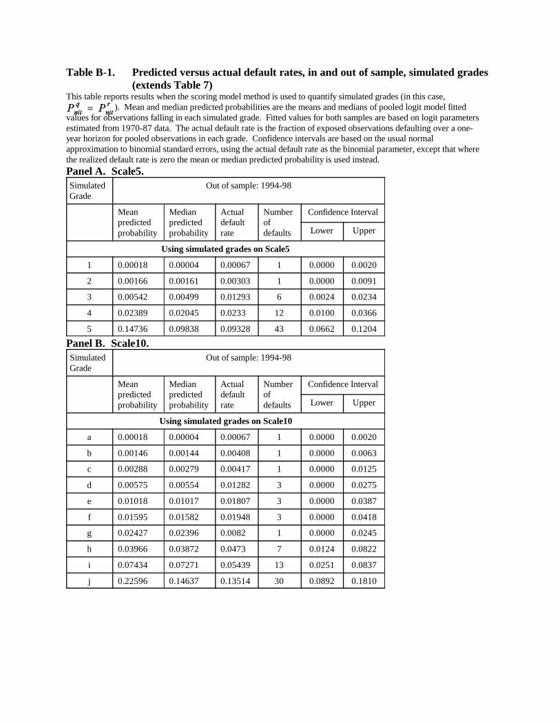
Table B-1. Predicted versus actual default rates, in and out of sample, simulated grades(extends Table 7)
This table reports results when the scoring model method is used to quantify simulated grades (in this case,). Mean and median predicted probabilities are the means and medians of pooled logit model fitted
values for observations falling in each simulated grade. Fitted values for both samples are based on logit parametersestimated from 1970-87 data. The actual default rate is the fraction of exposed observations defaulting over a one-year horizon for pooled observations in each grade. Confidence intervals are based on the usual normalapproximation to binomial standard errors, using the actual default rate as the binomial parameter, except that wherethe realized default rate is zero the mean or median predicted probability is used instead.Panel A. Scale5.SimulatedGrade
Out of sample: 1994-98
Meanpredictedprobability
Medianpredictedprobability
Actualdefaultrate
Numberofdefaults
Confidence Interval
Lower Upper
Using simulated grades on Scale5
1 0.00018 0.00004 0.00067 1 0.0000 0.0020
2 0.00166 0.00161 0.00303 1 0.0000 0.0091
3 0.00542 0.00499 0.01293 6 0.0024 0.0234
4 0.02389 0.02045 0.0233 12 0.0100 0.0366
5 0.14736 0.09838 0.09328 43 0.0662 0.1204
Panel B. Scale10.SimulatedGrade
Out of sample: 1994-98
Meanpredictedprobability
Medianpredictedprobability
Actualdefaultrate
Numberofdefaults
Confidence Interval
Lower Upper
Using simulated grades on Scale10
a 0.00018 0.00004 0.00067 1 0.0000 0.0020
b 0.00146 0.00144 0.00408 1 0.0000 0.0063
c 0.00288 0.00279 0.00417 1 0.0000 0.0125
d 0.00575 0.00554 0.01282 3 0.0000 0.0275
e 0.01018 0.01017 0.01807 3 0.0000 0.0387
f 0.01595 0.01582 0.01948 3 0.0000 0.0418
g 0.02427 0.02396 0.0082 1 0.0000 0.0245
h 0.03966 0.03872 0.0473 7 0.0124 0.0822
i 0.07434 0.07271 0.05439 13 0.0251 0.0837
j 0.22596 0.14637 0.13514 30 0.0892 0.1810

Table B-2. Model-predicted versus actual default rates, in and out of sample, Moody’sgrades (extends Table 9)
This table reports results when the scoring model method (logit model fitted values) is used to quantify Moody’sgrades. Mean and median predicted probabilities are the means and medians of pooled logit model fitted values forobservations falling in each grade. Fitted values for both samples are produced using logit parameters estimatedfrom 1970-87 data. The actual default rate is the fraction of exposed observations defaulting over a one-year horizonfor pooled observations in each grade. Confidence intervals are based on the usual normal approximation tobinomial standard errors, using the actual default rate as the binomial parameter, except that where the realizeddefault rate is zero the mean or median predicted probability is used instead.
Moody’sGrade
In estimation sample: 1970-87
Meanpredictedprobability
Medianpredictedprobability
Actualdefaultrate
Numberofdefaults
Confidence Interval
Lower Upper
Using simulated grades on Scale5
Aaa 0 0 0 0 0.0000 0.0000
Aa 0.00032 0 0 0 0.0000 0.0033
A 0.00088 0.00008 0 0 0.0000 0.0033
Baa 0.00668 0.00061 0.00155 1 0.0000 0.0046
Ba 0.01791 0.00302 0.00819 7 0.0020 0.0144
B 0.05607 0.02021 0.0394 34 0.0262 0.0526
C grades 0.13623 0.09921 0.19091 21 0.1160 0.2659
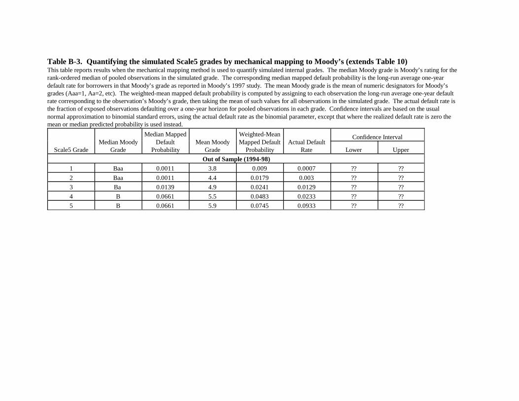
Table B-3. Quantifying the simulated Scale5 grades by mechanical mapping to Moody’s (extends Table 10)This table reports results when the mechanical mapping method is used to quantify simulated internal grades. The median Moody grade is Moody’s rating for therank-ordered median of pooled observations in the simulated grade. The corresponding median mapped default probability is the long-run average one-yeardefault rate for borrowers in that Moody’s grade as reported in Moody’s 1997 study. The mean Moody grade is the mean of numeric designators for Moody’sgrades (Aaa=1, Aa=2, etc). The weighted-mean mapped default probability is computed by assigning to each observation the long-run average one-year defaultrate corresponding to the observation’s Moody’s grade, then taking the mean of such values for all observations in the simulated grade. The actual default rate isthe fraction of exposed observations defaulting over a one-year horizon for pooled observations in each grade. Confidence intervals are based on the usualnormal approximation to binomial standard errors, using the actual default rate as the binomial parameter, except that where the realized default rate is zero themean or median predicted probability is used instead.
Scale5 GradeMedian Moody
Grade
Median MappedDefault
ProbabilityMean Moody
Grade
Weighted-MeanMapped Default
ProbabilityActual Default
Rate
Confidence Interval
Lower Upper
Out of Sample (1994-98)1 Baa 0.0011 3.8 0.009 0.0007 ?? ??
2 Baa 0.0011 4.4 0.0179 0.003 ?? ??
3 Ba 0.0139 4.9 0.0241 0.0129 ?? ??
4 B 0.0661 5.5 0.0483 0.0233 ?? ??
5 B 0.0661 5.9 0.0745 0.0933 ?? ??
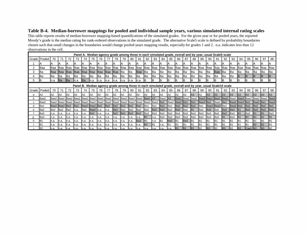
Table B-4. Median-borrower mappings for pooled and individual sample years, various simulated internal rating scalesThis table reports results of median-borrower mapping-based quantifications of the simulated grades. For the given year or for pooled years, the reportedMoody’s grade is the median rating for rank-ordered observations in the simulated grade. The alternative Scale5 scale is defined by probability boundarieschosen such that small changes in the boundaries would change pooled-years mapping results, especially for grades 1 and 2. n.a. indicates less than 12observations in the cell.
Panel A. Median agency grade among those in each simulated grade, overall and by year, usual Scale5 scaleGrade Pooled 70 71 72 73 74 75 76 77 78 79 80 81 82 83 84 85 86 87 88 89 90 91 92 93 94 95 96 97 98
1 A A A A A A A A A A A A A A A A A A A A A A A A A A A A A A2 Baa Baa Baa Baa Baa Baa Baa Baa Baa Baa Baa Baa Baa Baa Baa Baa Baa Baa Baa Baa Baa Baa Baa Baa Baa Baa Baa Baa Baa Baa3 Ba Baa Baa Baa Baa Baa Baa Baa Baa Baa Ba Ba Baa Ba Ba Ba Ba Ba Ba Ba Ba Ba Baa Ba Ba Ba Ba Ba Ba Ba4 Ba Ba Ba Ba Ba Ba Ba Ba Ba Ba Ba Ba Ba Ba Ba Ba Ba Ba Ba Ba Ba Ba Ba Ba Ba B B B B B5 B n.a Ba Ba n.a Ba n.a n.a n.a n.a n.a n.a n.a B B B B B B B B B B B B B B B B B
Panel B. Median agency grade among those in each simulated grade, overall and by year, usual Scale10 scaleGrade Pooled 70 71 72 73 74 75 76 77 78 79 80 81 82 83 84 85 86 87 88 89 90 91 92 93 94 95 96 97 98
a A2 A2 A2 A2 A2 A2 A2 A2 A2 A2 A2 A2 A2 A2 A2 A2 A2 A2 A2 A3 A2 A3 A3 A3 A3 A3 A3 A3 A3 A3b Baa2 Baa2 Baa2 Baa2 Baa2 Baa2 Baa2 Baa2 Baa2 Baa2 Baa2 Baa2 Baa2 Baa1 A3 Baa2 A3 Baa1 Baa2 Baa2 Baa3 Baa1 Baa1 Baa1 Baa2 Baa3 Baa2 Baa2 Baa2 Baa3c Baa2 Baa2 Baa2 Baa2 Baa2 Baa2 Baa2 Baa2 Baa2 Baa2 Baa2 Baa2 Baa2 Baa2 Baa2 Ba1 Baa2 Baa3 Ba1 Ba1 Baa3 Ba1 Baa2 Ba1 Baa3 Baa3 Ba1 Baa3 Ba1 Baa3d Ba1 Baa2 Baa2 Ba2 Ba2 Baa2 Baa2 Ba2 Ba2 Ba2 Ba2 Ba2 Ba2 Ba1 Ba1 Ba3 Ba1 Ba2 Ba2 Ba2 Ba1 Baa3 Baa3 Ba1 Baa3 Ba2 Ba2 Ba2 Ba2 Ba2e Ba2 Ba2 Ba2 Ba2 n.a. Ba2 Baa2 n.a. n.a. Ba1 Ba2 Ba2 Ba2 Ba2 Ba3 Ba3 Ba2 Ba3 Ba2 B1 Ba2 Ba3 Ba2 Ba3 Ba3 B1 Ba3 Ba3 Ba3 Ba3f Ba3 n.a. n.a. n.a. n.a. n.a. Ba2 n.a. n.a. Ba2 Ba2 Ba2 Ba2 Ba3 Ba3 Ba3 Ba3 Ba3 Ba3 Ba3 Ba3 Ba3 Ba3 Ba2 Ba3 B1 Ba3 B1 B1 Ba3g Ba3 n.a. n.a. n.a. n.a. n.a. n.a. n.a. n.a. n.a. n.a. n.a. n.a. B1 n.a. Ba3 Ba3 Ba3 Ba3 Ba3 Ba3 Ba3 Ba3 B1 Ba3 B1 B1 B1 B1 B1h B1 n.a. n.a. n.a. n.a. n.a. n.a. n.a. n.a. n.a. n.a. n.a. Ba2 B1 n.a. B1 Ba3 B1 Ba3 B1 B1 B1 B1 B1 B1 B1 B1 B1 B1 B1I B1 n.a. n.a. n.a. n.a. n.a. n.a. n.a. n.a. n.a. n.a. n.a. n.a. B3 B1 n.a. B1 B1 B1 B1 B1 B1 B1 B1 B1 B1 B1 B2 B2 B1j B2 n.a. n.a. n.a. n.a. n.a. n.a. n.a. n.a. n.a. n.a. n.a. n.a. n.a. n.a. n.a. n.a. B1 B1 B1 B2 B3 B2 B3 B2 B3 Caa1 B3 B3 B2
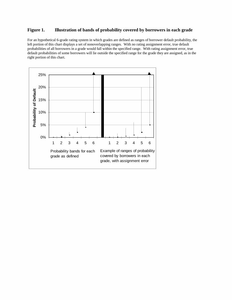
0%
5%
10%
15%
20%
25%
1 2 3 4 5 6 1 2 3 4 5 6
Pro
bab
ility
of
Def
ault
Probability bands for each grade as defined
Example of ranges of probability covered by borrowers in each grade, with assignment error
Figure 1. Illustration of bands of probability covered by borrowers in each grade
For an hypothetical 6-grade rating system in which grades are defined as ranges of borrower default probability, theleft portion of this chart displays a set of nonoverlapping ranges. With no rating assignment error, true defaultprobabilities of all borrowers in a grade would fall within the specified range. With rating assignment error, truedefault probabilities of some borrowers will lie outside the specified range for the grade they are assigned, as in theright portion of this chart.
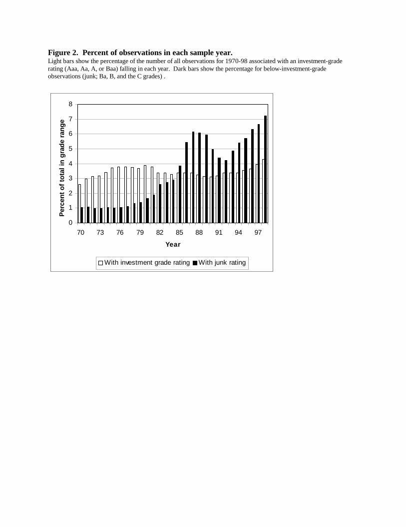
0
1
2
3
4
5
6
7
8
70 73 76 79 82 85 88 91 94 97
Year
Per
cen
t o
f to
tal i
n g
rad
e ra
ng
e
With investment grade rating With junk rating
Figure 2. Percent of observations in each sample year.Light bars show the percentage of the number of all observations for 1970-98 associated with an investment-graderating (Aaa, Aa, A, or Baa) falling in each year. Dark bars show the percentage for below-investment-gradeobservations (junk; Ba, B, and the C grades) .
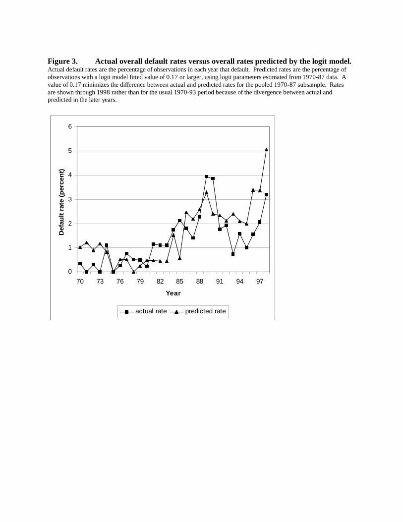
0
1
2
3
4
5
6
70 73 76 79 82 85 88 91 94 97
Year
Def
ault
rat
e (p
erce
nt)
actual rate predicted rate
Figure 3. Actual overall default rates versus overall rates predicted by the logit model.Actual default rates are the percentage of observations in each year that default. Predicted rates are the percentage ofobservations with a logit model fitted value of 0.17 or larger, using logit parameters estimated from 1970-87 data. Avalue of 0.17 minimizes the difference between actual and predicted rates for the pooled 1970-87 subsample. Ratesare shown through 1998 rather than for the usual 1970-93 period because of the divergence between actual andpredicted in the later years.
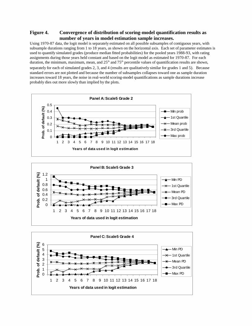
Panel A: Scale5 Grade 2
0
0.1
0.2
0.3
0.4
0.5
1 2 3 4 5 6 7 8 9 10 11 12 13 14 15 16 17 18
Years of data used in logit estimation
Pro
b. o
f d
efau
lt (
%)
Min prob
1st Quartile
Mean prob
3rd Quartile
Max prob
Panel B: Scale5 Grade 3
00.20.40.60.8
11.2
1 2 3 4 5 6 7 8 9 10 11 12 13 14 15 16 17 18
Years of data used in logit estimation
Pro
b. o
f d
efau
lt (
%)
Min PD
1st Quartile
Mean PD
3rd Quartile
Max PD
Panel C: Scale5 Grade 4
0123456
1 2 3 4 5 6 7 8 9 10 11 12 13 14 15 16 17 18
Years of data used in logit estimation
Pro
b. o
f d
efau
lt (
%)
Min PD
1st Quartile
Mean PD
3rd Quartile
Max PD
Figure 4. Convergence of distribution of scoring-model quantification results asnumber of years in model estimation sample increases.
Using 1970-87 data, the logit model is separately estimated on all possible subsamples of contiguous years, withsubsample durations ranging from 1 to 18 years, as shown on the horizontal axis. Each set of parameter estimates isused to quantify simulated grades (produce median fitted probabilities) for the pooled years 1988-93, with ratingassignments during those years held constant and based on the logit model as estimated for 1970-87. For eachduration, the minimum, maximum, mean, and 25th and 75th percentile values of quantification results are shown,separately for each of simulated grades 2, 3, and 4 (results are qualitatively similar for grades 1 and 5). Becausestandard errors are not plotted and because the number of subsamples collapses toward one as sample durationincreases toward 18 years, the noise in real-world scoring-model quantifications as sample durations increaseprobably dies out more slowly than implied by the plots.
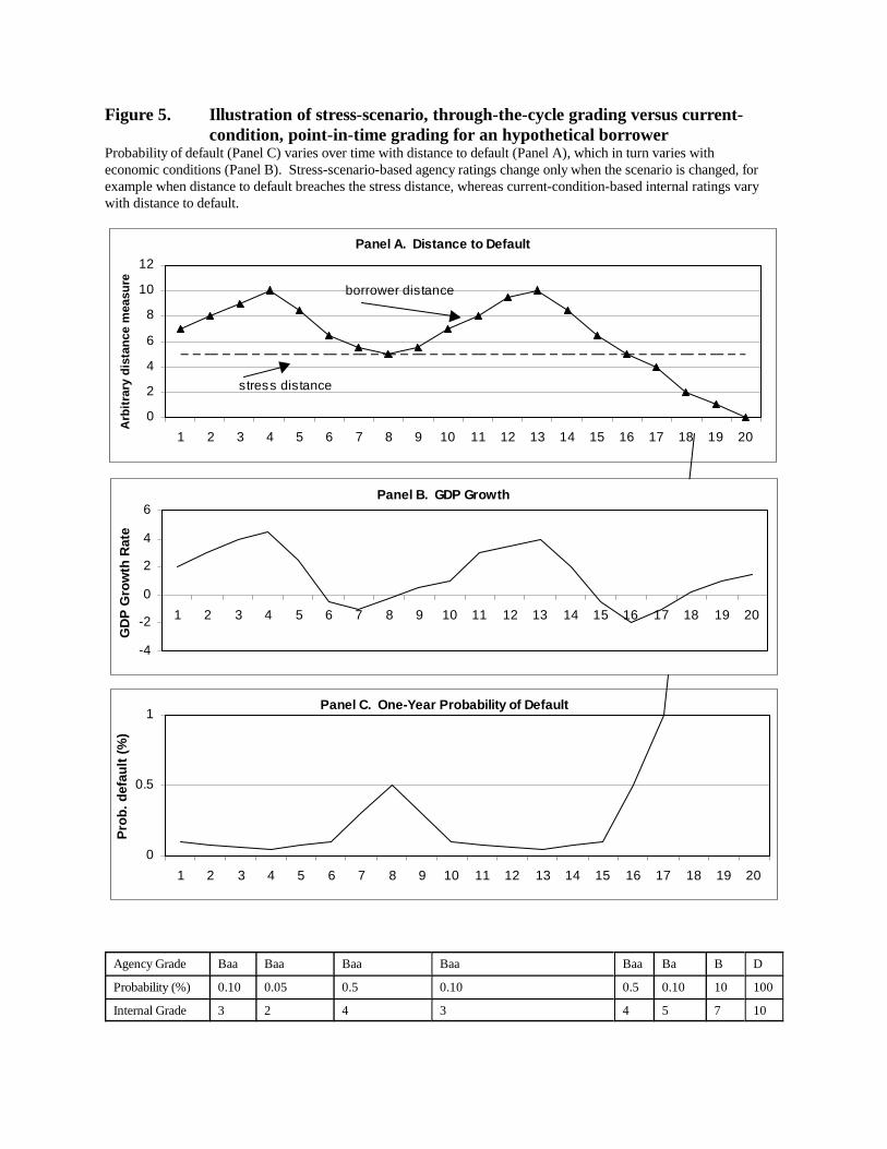
Panel A. Distance to Default
0
2
4
6
8
10
12
1 2 3 4 5 6 7 8 9 10 11 12 13 14 15 16 17 18 19 20
Arb
itra
ry d
ista
nce
mea
sure
stress distance
borrower distance
Panel C. One-Year Probability of Default
0
0.5
1
1 2 3 4 5 6 7 8 9 10 11 12 13 14 15 16 17 18 19 20
Pro
b. d
efau
lt (
%)
Panel B. GDP Growth
-4
-2
0
2
4
6
1 2 3 4 5 6 7 8 9 10 11 12 13 14 15 16 17 18 19 20
GD
P G
row
th R
ate
Figure 5. Illustration of stress-scenario, through-the-cycle grading versus current-condition, point-in-time grading for an hypothetical borrower
Probability of default (Panel C) varies over time with distance to default (Panel A), which in turn varies witheconomic conditions (Panel B). Stress-scenario-based agency ratings change only when the scenario is changed, forexample when distance to default breaches the stress distance, whereas current-condition-based internal ratings varywith distance to default.
Agency Grade Baa Baa Baa Baa Baa Ba B D
Probability (%) 0.10 0.05 0.5 0.10 0.5 0.10 10 100
Internal Grade 3 2 4 3 4 5 7 10
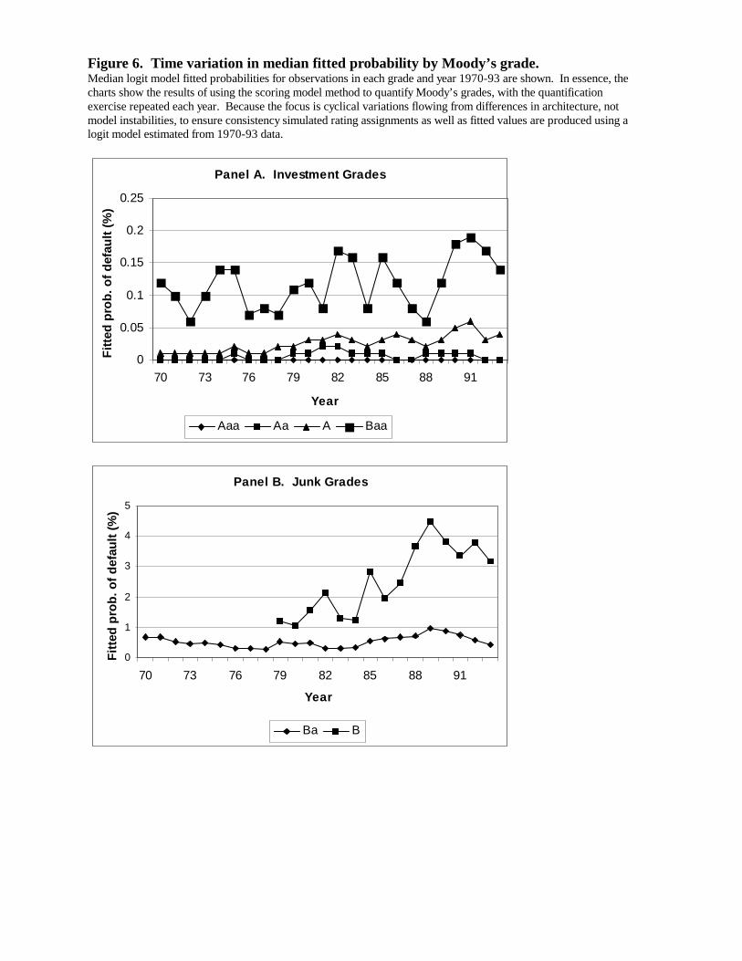
Panel A. Investment Grades
0
0.05
0.1
0.15
0.2
0.25
70 73 76 79 82 85 88 91
Year
Fit
ted
pro
b. o
f d
efau
lt (
%)
Aaa Aa A Baa
Panel B. Junk Grades
0
1
2
3
4
5
70 73 76 79 82 85 88 91
Year
Fit
ted
pro
b. o
f d
efau
lt (
%)
Ba B
Figure 6. Time variation in median fitted probability by Moody’s grade.Median logit model fitted probabilities for observations in each grade and year 1970-93 are shown. In essence, thecharts show the results of using the scoring model method to quantify Moody’s grades, with the quantificationexercise repeated each year. Because the focus is cyclical variations flowing from differences in architecture, notmodel instabilities, to ensure consistency simulated rating assignments as well as fitted values are produced using alogit model estimated from 1970-93 data.
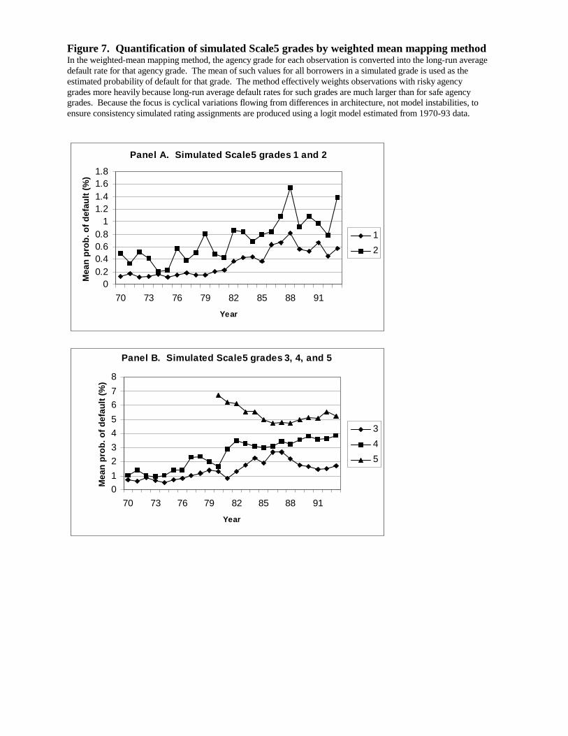
Panel A. Simulated Scale5 grades 1 and 2
00.20.40.60.8
11.21.41.61.8
70 73 76 79 82 85 88 91
Year
Mea
n p
rob
. of
def
ault
(%
)
1
2
Panel B. Simulated Scale5 grades 3, 4, and 5
0
1
2
3
4
5
6
7
8
70 73 76 79 82 85 88 91
Year
Mea
n p
rob
. of
def
ault
(%
)
3
4
5
Figure 7. Quantification of simulated Scale5 grades by weighted mean mapping methodIn the weighted-mean mapping method, the agency grade for each observation is converted into the long-run averagedefault rate for that agency grade. The mean of such values for all borrowers in a simulated grade is used as theestimated probability of default for that grade. The method effectively weights observations with risky agencygrades more heavily because long-run average default rates for such grades are much larger than for safe agencygrades. Because the focus is cyclical variations flowing from differences in architecture, not model instabilities, toensure consistency simulated rating assignments are produced using a logit model estimated from 1970-93 data.
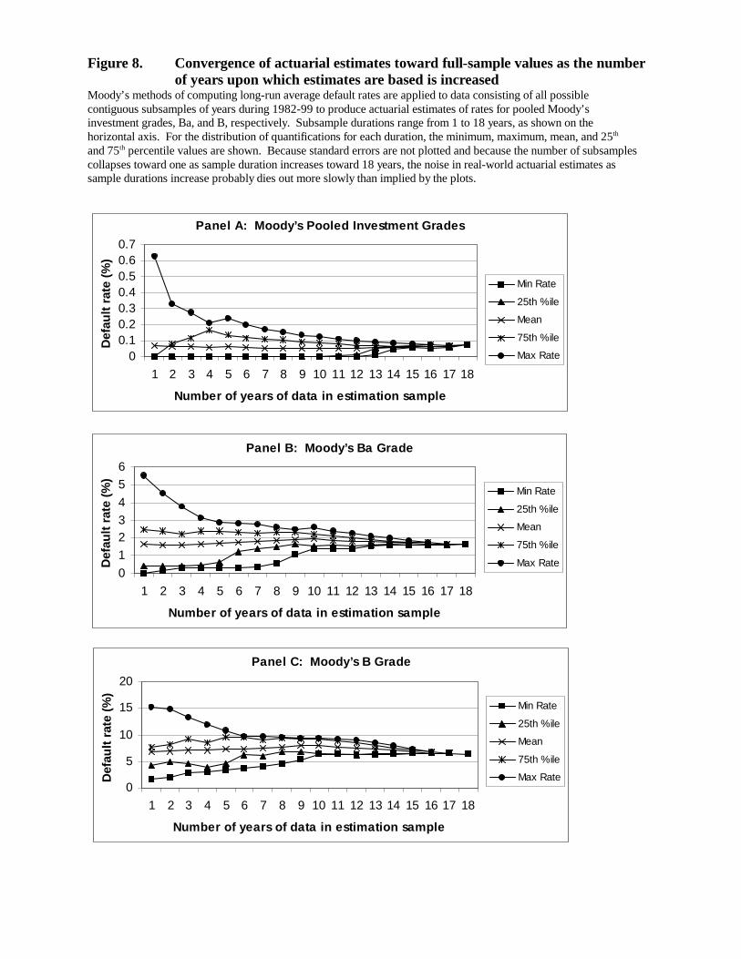
Panel B: Moody’s Ba Grade
0
1
23
4
5
6
1 2 3 4 5 6 7 8 9 10 11 12 13 14 15 16 17 18
Number of years of data in estimation sample
Def
ault
rat
e (%
)
Min Rate
25th %ile
Mean
75th %ile
Max Rate
Panel A: Moody’s Pooled Investment Grades
00.10.20.30.40.50.60.7
1 2 3 4 5 6 7 8 9 10 11 12 13 14 15 16 17 18
Number of years of data in estimation sample
Def
ault
rat
e (%
)
Min Rate
25th %ile
Mean
75th %ile
Max Rate
Panel C: Moody’s B Grade
0
5
10
15
20
1 2 3 4 5 6 7 8 9 10 11 12 13 14 15 16 17 18
Number of years of data in estimation sample
Def
ault
rat
e (%
)
Min Rate
25th %ile
Mean
75th %ile
Max Rate
Figure 8. Convergence of actuarial estimates toward full-sample values as the numberof years upon which estimates are based is increased
Moody’s methods of computing long-run average default rates are applied to data consisting of all possiblecontiguous subsamples of years during 1982-99 to produce actuarial estimates of rates for pooled Moody’sinvestment grades, Ba, and B, respectively. Subsample durations range from 1 to 18 years, as shown on thehorizontal axis. For the distribution of quantifications for each duration, the minimum, maximum, mean, and 25th
and 75th percentile values are shown. Because standard errors are not plotted and because the number of subsamplescollapses toward one as sample duration increases toward 18 years, the noise in real-world actuarial estimates assample durations increase probably dies out more slowly than implied by the plots.
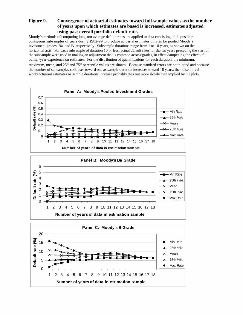
Panel A: Moody’s Pooled Investment Grades
0
0.1
0.2
0.3
0.4
0.5
0.6
0.7
1 2 3 4 5 6 7 8 9 10 11 12 13 14 15 16 17 18
Number of years of data in estimation sample
Def
ault
rat
e (%
)
Min Rate
25th %ile
Mean
75th %ile
Max Rate
Panel B: Moody’s Ba Grade
0
1
23
4
5
6
1 2 3 4 5 6 7 8 9 10 11 12 13 14 15 16 17 18
Number of years of data in estimation sample
Def
ault
rat
e (%
)
Min Rate
25th %ile
Mean
75th %ile
Max Rate
Panel C: Moody’s B Grade
0
5
10
15
20
1 2 3 4 5 6 7 8 9 10 11 12 13 14 15 16 17 18
Number of years of data in estimation sample
Def
ault
rat
e (%
)
Min Rate
25th %ile
Mean
75th %ile
Max Rate
Figure 9. Convergence of actuarial estimates toward full-sample values as the numberof years upon which estimates are based is increased, estimates adjustedusing past overall portfolio default rates
Moody’s methods of computing long-run average default rates are applied to data consisting of all possiblecontiguous subsamples of years during 1982-99 to produce actuarial estimates of rates for pooled Moody’sinvestment grades, Ba, and B, respectively. Subsample durations range from 1 to 18 years, as shown on thehorizontal axis. For each subsample of duration 10 or less, actual default rates for the ten years preceding the start ofthe subsample were used in making an adjustment that is common across grades, in effect dampening the effect ofoutlier-year experience on estimates. For the distribution of quantifications for each duration, the minimum,maximum, mean, and 25th and 75th percentile values are shown. Because standard errors are not plotted and becausethe number of subsamples collapses toward one as sample duration increases toward 18 years, the noise in real-world actuarial estimates as sample durations increase probably dies out more slowly than implied by the plots.
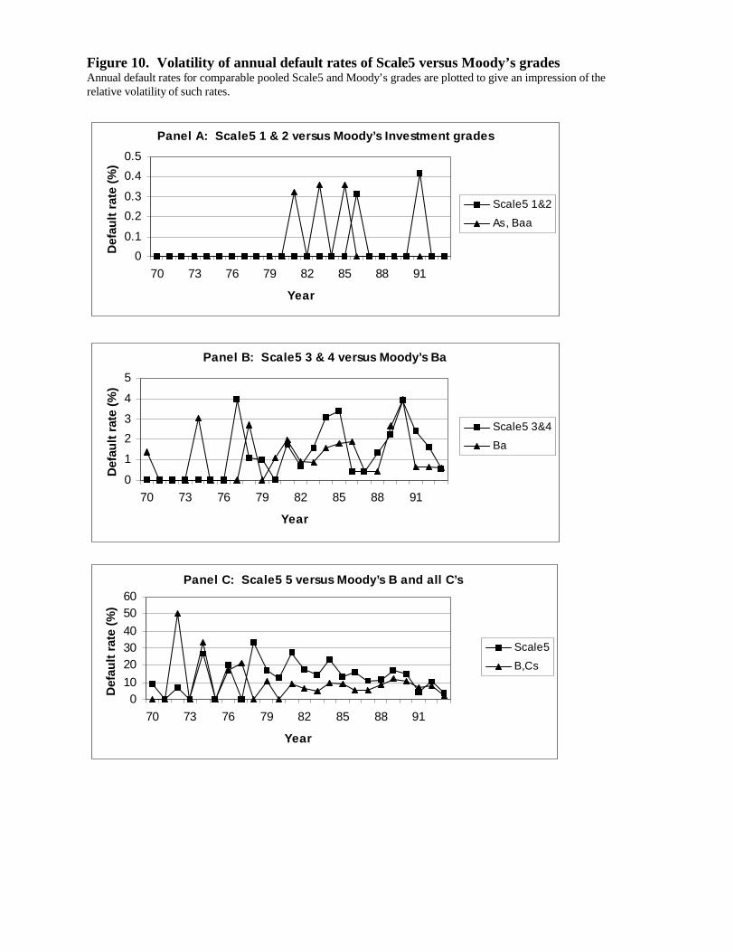
Panel A: Scale5 1 & 2 versus Moody’s Investment grades
0
0.1
0.2
0.3
0.4
0.5
70 73 76 79 82 85 88 91
Year
Def
ault
rat
e (%
)
Scale5 1&2
As, Baa
Panel B: Scale5 3 & 4 versus Moody’s Ba
0
1
2
3
4
5
70 73 76 79 82 85 88 91
Year
Def
ault
rat
e (%
)
Scale5 3&4
Ba
Panel C: Scale5 5 versus Moody’s B and all C’s
010
203040
5060
70 73 76 79 82 85 88 91
Year
Def
ault
rat
e (%
)
Scale5
B,Cs
Figure 10. Volatility of annual default rates of Scale5 versus Moody’s gradesAnnual default rates for comparable pooled Scale5 and Moody’s grades are plotted to give an impression of therelative volatility of such rates.
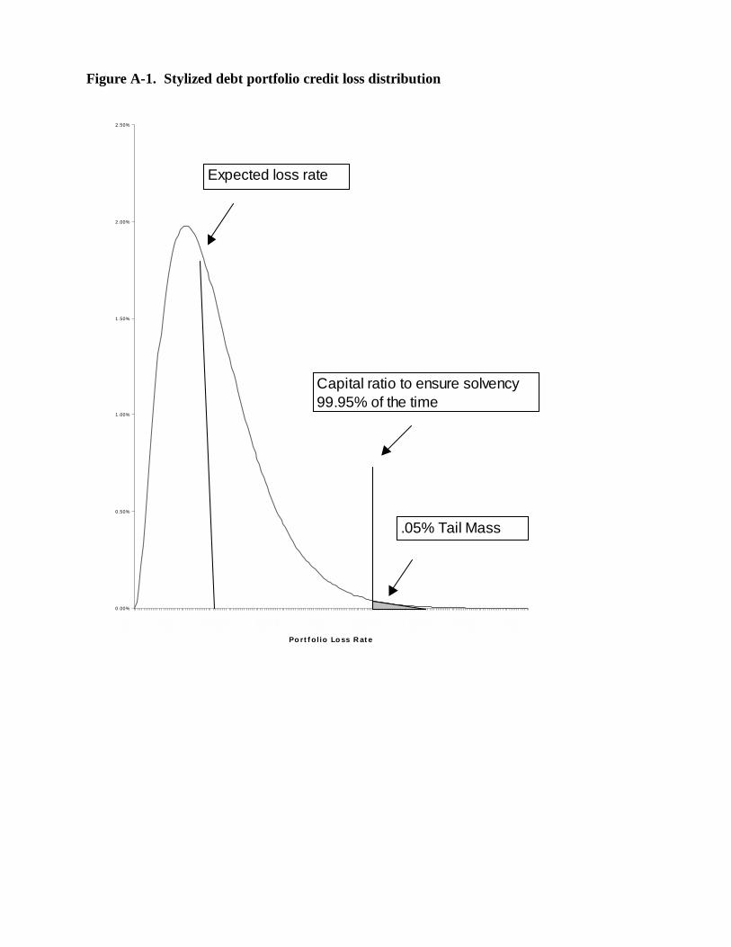
0.00%
0.50%
1.00%
1.50%
2.00%
2.50%
P or t f ol i o L os s R at e
.05% Tail Mass
Expected loss rate
Capital ratio to ensure solvency 99.95% of the time
Figure A-1. Stylized debt portfolio credit loss distribution