Embed Size (px)
Citation preview

Parameter OptimizationOf The Process
Of AA6xxx and AA7xxx seriesAluminium Extrusion
A THESIS PRESENTED IN FULFILMENT OF THE
REQUIREMENTS FOR THE DEGREE OF
DOCTOR OF PHILOSOPHY
IN
MECHANICAL ENGINEERING
AUCKLAND UNIVERSITY OF TECHNOLOGY,AUCKLAND
NEW ZEALAND.
Padmanathan Kathirgamanathan2013


Abstract
The mechanical properties and surface qualities of extruded aluminium products
depend greatly on the micro-structural changes during the extrusion process. A
clear understanding of the thermodynamics and tribology of the aluminium extru-
sion process with respect to the die design parameters and process parameters,
namely temperature and extrusion speed are necessary to decide the optimum
values of machine settings.
This research discusses the essential understanding of the process of alu-
minium extrusion, including the effects of die geometry and process parameters
on flow patterns. It presents the development of a technique to find an optimal
set of process and design parameter values for an isothermal process to extrude
a product for a given shape and material properties with minimal defects. The
inputs to this model are: the product geometry and its material data such
as flow curve and microstructure during dynamic recrystallization. This is
an inverse problem and the model is formulated as a non-linear least-squares
minimization problem coupled with a finite element model for the extrusion process.
The minimization problem where the geometry of a profile is simple is done
by constructing an iterative procedure using an optimization routine such as
MATLAB ’s lsqnonlin and at each iteration, the extrusion flow is solved using the
finite element programme ABAQUS. However, the die design parameters for a
complex geometry problem are different from a simple geometry problem. Further
ABAQUS is not very efficient to handle adaptive meshing for a complex thin
profile. The specialist finite element program DEFORM 3D for metal forming
applications, which efficiently uses adaptive meshing controls to accommodate high
iii

workpiece deformations, is used to overcome the problem. The optimal values of
the die design and process parameters are estimated by improving the techniques
available in the literature and compared with experimental results.
iv

Acknowledgements
First of all, I would like to express my sincere gratitude to my supervisor, Professor
Thomas Neitzert, for providing me an interesting industrial research problem to
work on. Thomas has been an exceptional advisor, both academically and person-
ally. His support, encouragement, suggestions, discussions and comments through-
out my research were invaluable. I was fortunate to have had the opportunity to
work with him.
I would also like to thank Professor Zhan Chen for his valuable comments on
various parts of my thesis. My thanks also extend to my colleague Florian Kern
for his continuous support and regular discussions.
My thanks also go to the Foundation for Research Science and Technology,
School of Engineering, as well as School of Computing and Mathematical Sciences
for financial supports.
v

vi
List of publications from this project
(i) Kathirgamanathan P., and Neitzert T., Optimization method of extrusion
dies with a thin and complex shape, Submitted to Australian Journal of
Mechanical Engineering.
(ii) Kathirgamanathan P., and Neitzert T., Optimization of pocket design to
produce a thin shape complex profile, Production Engineering Research &
Development, 3-3, 231–241, 2009.
(iii) Kathirgamanathan P., and Neitzert T., Inverse Modelling for Estimation of
Average Grain Size and Material Constants - An Optimization Approach,
Lecture Notes in Engineering and Computer Science, 2, 850–854, 2008.
(iv) Kathirgamanathan P., and Neitzert T., Optimal process control parameters
estimation in aluminium extrusion for given product characteristics, Lecture
Notes in Engineering and Computer Science, 2, 1436–1441, 2008.
(v) Kathirgamanathan P., and Neitzert T., Modelling of metal extrusion using
ABAQUS, The Proceedings of 3rd NZ Metals Industry Conference 2006.
vii

viii

Contents
Abstract iii
List of publications from this project vii
List of Symbols xiii
1 Introduction 1
1.1 Overview of Numerical Simulations of Aluminium Extrusion . . . . 1
1.2 The Problem Statement . . . . . . . . . . . . . . . . . . . . . . . . 3
1.2.1 Background . . . . . . . . . . . . . . . . . . . . . . . . . . . 3
1.2.2 The Main Project Goal . . . . . . . . . . . . . . . . . . . . . 3
1.2.3 Technical Target . . . . . . . . . . . . . . . . . . . . . . . . 4
1.3 The Scope of the Problem . . . . . . . . . . . . . . . . . . . . . . . 5
1.4 Overview of the Research . . . . . . . . . . . . . . . . . . . . . . . . 5
2 Metal Extrusion and Simulation 9
2.1 Introduction . . . . . . . . . . . . . . . . . . . . . . . . . . . . . . . 9
2.2 Theoritical Aspects of Extrusion . . . . . . . . . . . . . . . . . . . . 11
2.3 Microstructure Models . . . . . . . . . . . . . . . . . . . . . . . . . 14
2.4 Forward Problem of Extrusion Process . . . . . . . . . . . . . . . . 15
2.5 Finite Element Analysis . . . . . . . . . . . . . . . . . . . . . . . . 18
2.5.1 Introduction . . . . . . . . . . . . . . . . . . . . . . . . . . . 18
ix

2.5.2 Finite Element Formulation . . . . . . . . . . . . . . . . . . 20
2.6 Extrusion Defects . . . . . . . . . . . . . . . . . . . . . . . . . . . . 27
2.7 Previous Work . . . . . . . . . . . . . . . . . . . . . . . . . . . . . 31
2.8 Unresolved Issues . . . . . . . . . . . . . . . . . . . . . . . . . . . . 42
2.9 The Research Strategy and Methodology . . . . . . . . . . . . . . . 43
3 FEA Modelling of Extrusion 47
3.1 Overview . . . . . . . . . . . . . . . . . . . . . . . . . . . . . . . . . 47
3.2 DEFORM . . . . . . . . . . . . . . . . . . . . . . . . . . . . . . . . 48
3.3 Modelling Process in DEFORM . . . . . . . . . . . . . . . . . . . . 49
3.4 ABAQUS . . . . . . . . . . . . . . . . . . . . . . . . . . . . . . . . 52
3.5 Modelling Process in ABAQUS . . . . . . . . . . . . . . . . . . . . 53
3.6 Simulation of Extrusion Process . . . . . . . . . . . . . . . . . . . . 58
3.6.1 Flow Simulation . . . . . . . . . . . . . . . . . . . . . . . . . 58
3.6.2 Die Design Parameters . . . . . . . . . . . . . . . . . . . . . 60
3.6.3 Inaccuracy of Material Properties . . . . . . . . . . . . . . . 64
3.6.4 Computational Issues . . . . . . . . . . . . . . . . . . . . . . 68
3.7 Discussion . . . . . . . . . . . . . . . . . . . . . . . . . . . . . . . . 73
4 Optimal Process and Design Parameters Estimation for a Simple
Die 75
4.1 Introduction . . . . . . . . . . . . . . . . . . . . . . . . . . . . . . . 75
4.2 Forward Problem . . . . . . . . . . . . . . . . . . . . . . . . . . . . 76
4.3 Inverse Problem . . . . . . . . . . . . . . . . . . . . . . . . . . . . . 77
4.3.1 Design Variables . . . . . . . . . . . . . . . . . . . . . . . . 78
4.3.2 Process Variables . . . . . . . . . . . . . . . . . . . . . . . . 78
4.4 Important Factors in the Product Optimization . . . . . . . . . . . 79
4.4.1 Die Life . . . . . . . . . . . . . . . . . . . . . . . . . . . . . 79
x

4.4.2 Isothermal Extrusion . . . . . . . . . . . . . . . . . . . . . . 82
4.4.3 Flow Balance . . . . . . . . . . . . . . . . . . . . . . . . . . 83
4.4.4 Distortion . . . . . . . . . . . . . . . . . . . . . . . . . . . . 86
4.4.5 Grain Size . . . . . . . . . . . . . . . . . . . . . . . . . . . . 89
4.5 Objective and Constraint Function . . . . . . . . . . . . . . . . . . 91
4.6 Schema of the Design . . . . . . . . . . . . . . . . . . . . . . . . . . 93
4.7 Results and Discussion . . . . . . . . . . . . . . . . . . . . . . . . . 95
4.8 Summary . . . . . . . . . . . . . . . . . . . . . . . . . . . . . . . . 99
5 Estimation of Average Grain Size and Material Constants 103
5.1 Introduction . . . . . . . . . . . . . . . . . . . . . . . . . . . . . . . 103
5.2 Forward Problem . . . . . . . . . . . . . . . . . . . . . . . . . . . . 105
5.3 Inverse Problem . . . . . . . . . . . . . . . . . . . . . . . . . . . . . 105
5.4 Applications . . . . . . . . . . . . . . . . . . . . . . . . . . . . . . . 108
5.4.1 Estimation of Grain Size d(t) for Known Value of Activation
Energy Q . . . . . . . . . . . . . . . . . . . . . . . . . . . . 110
5.4.2 Estimation of d(t) for Unknown Value of Activation Energy 113
5.5 Summary and Conclusion . . . . . . . . . . . . . . . . . . . . . . . 114
6 Optimization of Pocket Design to Produce a Thin Shape Complex
Profile 117
6.1 Introduction . . . . . . . . . . . . . . . . . . . . . . . . . . . . . . . 117
6.2 Finite Element Model . . . . . . . . . . . . . . . . . . . . . . . . . . 118
6.3 Analysis of the Influence of Pocket Design Parameters . . . . . . . . 122
6.3.1 Influence of Distance from Die Centre rp . . . . . . . . . . . 122
6.3.2 Influence of Pocket Shape . . . . . . . . . . . . . . . . . . . 124
6.3.3 Influence of Pocket Angle . . . . . . . . . . . . . . . . . . . 125
6.3.4 Influence of Channel Length . . . . . . . . . . . . . . . . . . 126
xi

6.4 Proposed Optimization Algorithms . . . . . . . . . . . . . . . . . . 128
6.4.1 Algorithm -1 . . . . . . . . . . . . . . . . . . . . . . . . . . 128
6.4.2 Algorithm -2 . . . . . . . . . . . . . . . . . . . . . . . . . . 129
6.5 Die with Feeder (or Welding) Chamber . . . . . . . . . . . . . . . . 135
6.5.1 Algorithm -3 . . . . . . . . . . . . . . . . . . . . . . . . . . 139
6.6 Summary and Discussion . . . . . . . . . . . . . . . . . . . . . . . . 141
7 Comparison with Experimental data 145
7.1 Experimental Trial . . . . . . . . . . . . . . . . . . . . . . . . . . . 145
7.2 Investigation of Product Surface . . . . . . . . . . . . . . . . . . . . 147
7.3 Image processing tool box - Matlab . . . . . . . . . . . . . . . . . . 155
7.4 Validation of FEA calculation . . . . . . . . . . . . . . . . . . . . . 158
7.5 Summary and Discussion . . . . . . . . . . . . . . . . . . . . . . . . 158
8 Summary and Conclusions 161
8.1 Summary . . . . . . . . . . . . . . . . . . . . . . . . . . . . . . . . 161
8.2 Conclusions . . . . . . . . . . . . . . . . . . . . . . . . . . . . . . . 164
8.3 Future Experimental work . . . . . . . . . . . . . . . . . . . . . . . 166
8.4 Future Research . . . . . . . . . . . . . . . . . . . . . . . . . . . . . 167
A Appendix: Programming Codes 169
Bibliography 177
xii

List of Symbols
Q activation energy [Jmol−1K−1]
davg average recrystallized grain size [m]
b bearing length [m]
Γ boundary
k conductivity [Sm−1]
εc critical strain
A cross sectional area [m2]
ρ density of the metal [kgm−3]
d depth of pocket [m]
θ die semi-cone angle [degrees]
rp distance between pocket axis and die axis [m]
x, y, z distances measured in the X, Y and Z directions respectively [m]
Ω domain˙ε effective strain-rate [s−1]
σ effective stress [Pa]
Pe extrusion pressure
V extrusion speed [ms−1]
σ flow stress [Pa]
µ friction factor
R gas constant [Jmol−1K−1]
qn heat flux [Wm−2]
q heat generation term [Ws−1]
d0avg initial grain size [m]
m, n material constants˙εave mean strain-rate of the deformation zone [s−1]
εi normal strain-rate in the i direction [s−1]
σi normal stress in the i direction [Pa]
ε0.5 plastic strain for 50% recrystallization
R0 radius of the billet [m]
Re radius of the extrudate or the die radius [m]
Cp specific heat capacity [Jkg−1K−1]
ε strain
t time [s]
vi velocity components in the i direction [ms−1]
χ volume fraction recrystallized
w, w1, w2 width of pockets [m]
xiii

xiv

Chapter 1
Introduction
1.1 Overview of Numerical Simulations of Alu-
minium Extrusion
Aluminium extrusion is a common forming process worldwide. Extrusion produces
a long profile of fixed cross-sectional area by pressing a hot billet through a hole
with a certain shape. Both mechanical properties and surface quality of the ex-
truded product depend mainly on initial billet temperature, extrusion speed and
die geometry. If the speed is high, the temperature goes up due to faster plas-
tic deformation and increased surface friction. This leads to surface defects on the
product. Homogeneity of flow also influences the product quality. The flow velocity
of every material particle in the cross-section across the die exit should be uniform
for achieving products with minimal defects. The geometry of the die opening
makes up an important feature of die design. It determines the homogeneity of
flow and the amount of redundant work done during the deformation process. A
profile, which minimizes the redundant work, will minimize the extrusion power.
The knowledge of the temperature distribution, velocity distribution inside the
forming zone and extrusion load is also very important for the determination of the
1

right extrusion process conditions.
The aim of any manufacturing process is the production of a steady quality
product at a minimal cost. Generally effective goals include shortening the lead time
in the design cycle, reducing tooling cost and machine downtime at the production
stage, and developing a stable process with a minimal reject rate. In practice, die
designers usually meeting their objective through trial and error methods. These
methods are time consuming and expensive. Sometimes dies have to be discarded
if it is difficult to rectify mistakes. This design process does not suit a modern
industrial environment.
By using numerical simulation for an extrusion process and predicting material
flow, the information of the material deformation, stress, strain, strain rate and
temperature distribution inside the extrusion die can be obtained. This method
will allow us to determine
1. whether a part can be formed without defects,
2. equipment forces and die stresses,
3. ways to reduce costly trials of proposed die designs,
4. ways to improve die designs to reduce production and material costs,
5. ways to minimize lead-time in bringing a new product to market.
This is an ongoing trend of modern manufacturing in the current industrial environ-
ment. As a simulation tool finite element modelling is a well-established numerical
technique for manufacturing processes and has been gaining wider acceptance over
the last several years.
2

1.2 The Problem Statement
1.2.1 Background
The current theoretical understanding of the extrusion process, its impact on the
tooling technology, extruded product and overall yield are somewhat limited. This
constraint not only restricts progress of making the existing production set-ups more
reliable and running at an optimum level but also doesn’t allow major advances of
new processes as well as product developments.
The lack of the ability to reliably simulate the extrusion process leads to sub-
optimum tooling designs and longer than necessary trial periods until a new tool
runs to satisfaction. Product designs are restricted by the standard of current
tool-design. Improved machine control strategies cannot be developed because the
relationships between process and material conditions aren’t well understood.
1.2.2 The Main Project Goal
The novel concept of this research is to
1. Determine the optimal process (ram speed, initial billet and die temperature)
and design (die shape) parameter values to get a
(i) High quality product in terms of
(a) homogeneity,
(b) uniform flow,
(c) material properties(average grain size),
(ii) With minimal defects such as
(a) surface defects (eg. flow lines),
(b) internal cracks (eg. central bursts also known as chevrons in extru-
sion).
3

2. Identify the process parameters which are more sensitive to product defects.
3. Improve the theoretical understanding of the process of aluminium extru-
sion through a simulation of the forming process and the related changes in
material structure.
Tool design and process control in the metal extrusion industry are still treated to
some extent by a trial and error approach, which will be overcome by this project
with the associated gains in reduced set-up time, improved process performance
and efficiency of operation.
The numerical simulation of extrusion using the finite element method is the
most promising option to replace the traditional trial and error as well as other
analytical methods. A finite element model, which is capable of describing the
behavior of metal flow during extrusion, requires several input data such as die
geometry, material behavior laws, friction laws and operating conditions. In reality,
material behavior can be obtained, but the die geometry, process conditions and
appropriate friction values to achieve a profile with given material properties are
often unknown.
1.2.3 Technical Target
The project will improve knowledge of the extrusion process and will lead to better
tool designs, increase of die life before failure and increase of surface quality of the
extruded product. The optimized die designs are also leading to reduced die costs.
The time spent on designing new tools will be reduced significantly. The outcome
of new product shapes which could not be attempted before and quality is difficult
to quantify, but will certainly strengthen the competitive situation of commercial
entities.
4

1.3 The Scope of the Problem
This research has relevance to the following:
(i) Improvement of the physical properties of the extruded material;
(a) products with high quality in terms of homogeneity, uniform flow and
given material properties.
(b) products with minimal defects such as surface defects, internal cracks
and central bursts.
(ii) Optimization of the cost of metal extrusion;
(a) maximize die life,
(b) minimize usage of energy,
(c) minimize time of die trials.
1.4 Overview of the Research
The aim of this research is to present a numerical model capable of predicting
an optimal set of conditions to extrude a product for a given shape and material
properties with minimal defects. The presentation of this report is organized into
8 chapters including the present.
Chapter 2 consists of the main literature review. It contains background ma-
terial for the numerical simulation of metal extrusion in general. An overview of
the extrusion process, modelling of the metal extrusion process, and numerical
techniques are described in the first three sections. Common forms of defects in
extrusion processes are also explained. The last two sections of the chapter con-
sider related problems and the work to be done to improve the extrusion process
in general.
5

In Chapter 3 the simulation of the extrusion process using finite element mod-
elling is introduced. This chapter starts with a brief description of finite element
softwares Abaqus and DEFORM 3D which are used for the investigation. In the sec-
ond half of the chapter, a small scale extrusion model is simulated using ABAQUS
and it is demonstrated how temperature, stress, strains and velocity changes dur-
ing the extrusion and how these quantities are related to die angle, die land length,
friction, material properties, initial billet temperature and extrusion speed. In ad-
dition ways to increase the efficiency in terms of using different solution schemes,
adaptive meshing, element type and different contact algorithms are described. The
aim of this chapter is to understand the extrusion process in general and ways to
solve extrusion problems more efficiently.
Chapter 4 investigates a numerical technique to estimate the optimal die pro-
file and the process parameters such as extrusion speed and initial temperatures
simultaneously. This chapter provides a detailed description of an inverse model
capable of simultaneously estimating die design and process parameters. In addi-
tion, a series of examples are considered to describe how optimal values of design
and process parameters can be determined and how changes in these values will
influence optimization criteria.
The objective of Chapter 5 is to describe an inverse model capable of con-
currently estimating the average grain size, activation energy and other material
constants appearing in the model. The chapter starts with the description of the
forward problem, difficulties with the forward problem and the data requirements
for the inverse problem. Then the methodology of the inverse problem for estimat-
ing parameter values by using simulated strain and temperature values at a single
node is presented.
Chapter 6 investigates the influence of shape, depth, and widths of a pocket to
regulate the metal flow through a more complex thin die with varying thickness.
6

The chapter starts with the simulation of extrusion through a complex die which is
currently in commercial use and analyzes the reasons for insufficient surface quality
of the extruded product. Next, the methodology to improve the surface quality
of the extruded product is presented, which includes the analysis of pocket design
parameters and algorithms. Finally some numerical simulation results are presented
to compare the newly designed die with the original die.
In Chapter 7, experimental data using the newly designed die and the original
die are presented. This chapter describes the equipment, trial procedure and sample
preparation as well as evaluation.
Chapter 8 presents the summary, conclusion and possible extension of this
project.
This thesis includes information already published in [33], [34], [35] and [36].
7

8

Chapter 2
Metal Extrusion and Simulation
2.1 Introduction
Extrusion is a plastic deformation process in which a block of metal (billet) is com-
pressed through a die opening of a smaller cross sectional area than that of the
original billet as shown in Figure (2.1). During the process, heat is generated by
both the frictional work and deformation work. This heat is transported with the
extruded material while conduction, convection and radiation take place simultane-
ously. In broad terms some of the generated heat remains in the extruded material,
some is transmitted to the container and die and some increases the temperature
of the part of the billet that is not yet extruded.
It is a thermo-mechanical process and it involves interaction between the process
parameters, tooling and deformed material. The whole process is composed of two
distinctly different stages, namely the transient state at the beginning and steady
state of the rest of the cycle. Further the wear process on the die bearing is
dependent on the thermodynamics of extrusion which is very much influenced by
the effects of extrusion variables. The tribology in metal extrusion has a direct
influence on the accuracy of the shape and the surface finish of the workpiece.
9

Figure 2.1: Machinery set up at the factory [[73]]
There are five main types of extrusion[65]:
1. Direct extrusion: A press pushes the ram on one end and the extrudate is
forced through the die on the other end.
2. Indirect extrusion (or backwards extrusion): It involves a stationary billet
with a moving die.
3. Hydrostatic extrusion: It is using a fluid to hydrostatically pressurize the
material out of the container.
4. Impact extrusion: This is a high speed process for creating hollow shapes like
soda cans.
5. Extrusion with active friction: In this process the extrusion die remains sta-
tionary while the ram and container move in the direction of flow. The
benefits are improved homogeneity of metal flow, higher speeds and no metal
flow interface at the container bottom[39].
10

In the extrusion process, the large deformations are mainly plastic or viscoplastic.
The elastic component is very small and neglected. neglected. Therefore the the-
ory of plasticity is used in metal forming processes to investigate and study the
mechanics of extrusion. This will allow us
1. to analyse and predict the flow pattern, temperature, heat transfer, variation
of local material strength, stresses, forming load, pressure and energy, and
2. to study how the metal flow during extrusion depends on material proper-
ties and initial billet temperature, ram speed, friction between billet and die
surface and extrusion ratio.
2.2 Theoritical Aspects of Extrusion
To study the extrusion process in detail, the strain, strain rate, material flow stress,
and friction between the interfaces are important. These can be defined as follows
1. The strain [ε]: It is a measure of deformation. There are two types. They are
defined by
Engineering strain =Change in length
Original length(2.1)
True strain = ln
(1 +
Change in length
Original length
)(2.2)
2. The stress [σ]: It is a measure of force applied to a unit area of material,
σ =F
A.
3. The strain rate [ε]: It is a measure of the instantaneous rate of deformation
a region of material is experiencing. The general definition would be ε =dε
dt.
The mean strain rate may be computed from
˙εm = ε6vD2
0 tan θ
D30 −D3
1
, (2.3)
11

where v is ram velocity, θ is the semi-cone angle of the die entry, D0 is the
initial diameter of billet and D1 is the final diameter of extruded product.
4. Material Flow Stress: It is a true stress-strain curve and is commonly called
flow curve. It gives the stress required to cause the metal to flow plasti-
cally at any given strain. Different methods of mathematically defining the
relationship are given in the literature. Some of them are
Method 1
σ = cεn ˙εm
+ y (2.4)
where σ is the flow stress, ε is the effective plastic strain, ˙ε is the effective
strain rate, c is a material constant, n is the strain hardening exponent,
m is the strain rate exponent and y is an initial yield value.
Method 2
˙ε = γ (sinh (ασ))n1 exp
(− Q
RT
)(2.5)
where γ, α are constants, n1 is the strain rate exponent, Q is the acti-
vation energy, R is the gas constant, and T is the absolute temperature,
σ is the flow stress, and ˙ε is the effective strain rate.
Method 3
˙ε = γσn exp
(− Q
RT
)(2.6)
where γ is a constant, and n is the strain rate exponent.
5. Friction: It is the resistance to relative motion that is experienced whenever
two surfaces are in contact with one another. The friction components for
the direct extrusion process are
(i) Billet-Container interface
(ii) Dead-metal zone metal interface
12

(iii) Die-material interface
The friction models being used for the extrusion process can be divided into
three different categories. They are classic friction models, the empirical fric-
tion models and the physically based friction models. The Coulomb friction
model and Shear friction model are the two classic friction models. The fric-
tional force in the constant shear model is defined by
fs = µk (2.7)
where fs is the frictional stress, k is the shear yield stress and µ is the friction
factor. Coulomb friction is used when contact occurs between two elasti-
cally/plastically deforming objects or an elastic object and a rigid object.
The frictional force in the Coulomb law model is defined by
fs = µp (2.8)
where fs is the frictional stress, p is the interface pressure between two bodies
and µ is the friction factor.
The friction stress calculated using the Coulomb friction model may be higher
than the shear flow stress of the workpiece material due to the high contact
pressure at the workpiece-die interface. To avoid the overestimation of friction
stress, the shear friction model may be an answer. But it is not easy to
estimate the value of friction experimentally and therefore the selection of
friction values can be guesswork. The empirical friction models are mainly
based on experimental observations and the model parameters are normally
related to extrusion speed and billet temperature. In physically based friction
models, the friction force is considered as a summation of ploughing forces
13

generated from joined contact patches.
A comparative study of friction models for hot aluminium extrusion processes
has been conducted by Wang and Yang [79] and have shown that the full
sticking friction appeared to represent the interfacial contact between the
hot aluminium and the die the best. Therefore, in FE simulations of hot
aluminium extrusion, the classic friction models, with m or µ at or close to
unity could be assigned as friction boundary condition at the workpiece/die
interface. This is not only for saving computing time, but also for avoiding
convergence problems.
6. The redundant work: Due to inhomogeneity of flow through the die, extra
work is needed to deform the material to the final shape. The redundant work
is approximately proportional to the strain ε and the extrusion pressure Pe
and is approximately equal to [65]
Pe = σ (0.8 + 1.2ε) (2.9)
2.3 Microstructure Models
In extrusion as in any other manufacturing processes, product quality is an impor-
tant cost factor. The product properties are closely related to the uniformity of
the microstructure. There are various microstructure models [[9], [10], [11], [53]]
available, which are based on laboratory observations. One example is the relation-
ship between microstructural parameters (the average recrystallized grain size d,
volume fraction recrystallized (χ) and process parameters (ε, T , and ε)) developed
14
by Malas [53], which are given by
χ = 1− exp
(log(2)
(ε− εcε0.5
)2), (2.10)
εc = 4.76× 10⁻⁴ exp(8000
T), (2.11)
ε0.5 = 1.144× 10⁻³d0.280 ε0.05 exp
(6420
T
), (2.12)
d = 22600ε−0.27 exp
(−0.27
Q
RT
), (2.13)
where εc = critical strain, ε0.5 = plastic strain for 50% recrystallization, d0 =
initial grain size, activation energy Q = 310 kJ/mol and gas constant R = 8.314×
10−3 kJ/mol −K.
2.4 Forward Problem of Extrusion Process
Extrusion is a thermo-mechanical deformation process in which a block of metal
(billet) is forced through the die opening of a smaller cross sectional area than that
of the original billet. In this process, the large deformations are mainly plastic or
viscoplastic, allowing the elastic part to be neglected. Therefore a rigid-viscoplastic
formulation can be adopted. Strain is a measure of deformation and at high strain
rates metal flow is analogous to fluid flow[5]. Therefore the material behavior can
be described as that of fluid flow as in [5], [12], [38], [59], [70]
(i) Conservation of mass: The law states that the rate of change of mass in a
fixed region is zero.
ρ+ ρDij = 0 (2.14)
where ρ is the density of the material and
Dij =1
2
(∂vi∂xj
+∂vj∂xi
)in Ω (2.15)
15

is the deformation tensor. If the material is incompressible, density is un-
changed and the Equation (2.14) is simplified to
Dij = 0. (2.16)
(ii) Conservation of momentum: It says that the rate of change of momentum is
equal to the sum of external forces acting on the region.
ρvi = ρfi + σij,j in Ω (2.17)
where f is the body force per unit mass, and σ is the Cauchy stress tensor.
It has been assumed that ρvi ≈ 0. Boundary conditions are
σijnj = ti on Γt (2.18)
vi = vi on Γv (2.19)
Here, the domain Ω and its associated boundary Γ represent the current
configuration of the body. Γt and Γv represent respectively, the part of the
boundary Γ where traction and velocities are prescribed. n is the outward
normal vector at the interfacial surface. Indices i, j, k are used to denote the
components of the tensor and an apostrophe denotes the spatial derivatives
with respect to the current configuration. The constitutive equation is
σ′ij = 2γDij (2.20)
where γ =σ
3˙ε, σ′ is the deviatoric stress tensor, σ is the effective stress and
˙ε is the effective strain rate.
16

The Yield criterion is:
σ(ε, ˙ε, T ) =
√3
2σ′ijσ
′ij, (2.21)
˙ε =
√2
3˙εij ˙εij. (2.22)
(iii) Conservation of energy: It says that the rate of change of the total energy is
equal to the sum of the rate of work done by applied forces and the change
of heat content per unit time.
ρCp
(∂T
∂t+ vr
∂T
∂r+ vz
∂T
∂z
)=
1
r
∂
∂r
(rk∂T
∂r
)+
∂
∂z
(k∂T
∂z
)+ q (2.23)
and the boundary conditions are
T = T on ΓT (2.24)
(k∂T
∂r− ρCpvrT
)nr +
(k∂T
∂z− ρCpvzT
)nz = qn on Γq (2.25)
Initial Condition is
T (r, z, 0) = T0(r, z) (2.26)
where q, qn, T , k, ρ, and Cp are the heat rate generation term, heat flux
normal to the boundary surface, temperature, conductivity, density, and spe-
cific heat of the material in that order. ΓT and Γq represent respectively the
temperature prescribed surface and the surface where heat transfer occurs.
The exact mathematical analysis of the extrusion process is quite complex and has
not been fully resolved. Therefore in recent years, many numerical methods using
finite element techniques have been reported in the literature[[8], [26], [28], [38],
[50]].
17

2.5 Finite Element Analysis
2.5.1 Introduction
When a problem is impossible to solve using analytical techniques, numerical tech-
niques can be used to obtain a solution. One of the popular numerical techniques
is finite element analysis (FEA). It is a very common method for metal forming
processes including extrusion and a suitable method for any problem with arbi-
trary geometry. The finite element formulation of a problem results in a system of
simultaneous algebraic equations.
There are three different types of finite element formulations used in modeling
metal forming processes. They are Lagrangian, Eulerian and arbitrary Lagrangian
Eulerian (ALE) formulations. The selection of type is based on the problem to be
solved and to some extent the computer resources available.
In Lagrangian formulation, the mesh moves with the material and deforms with
the flow of material. In Eulerian formulation nodes and elements are fixed in space
and the material flows through the mesh. The major advantage of this formulation
is that problems related to mesh distortion are avoided. In this formulation a prob-
lem with large deformations can be modeled with very low computational cost. The
ALE methods are arbitrary combinations of the Lagrangian and Eulerian formula-
tions and were developed in an attempt to bring the advantages of both Lagrangian
and Eulerian formulation together. In an ALE formulation the displacements of
material and mesh are decoupled and the mesh can move independently of the
material.
The solution methods of finite element analysis can generally be grouped as
either implicit or explicit. The choice of solution methods depends on the model,
computational resources and nonlinearity of the system. It is typically solved in-
crementally.
18

In the implicit approach the state of a finite element model is updated from time
t to t+ ∆t. The state at t+ ∆t is determined based on information at time t+ ∆t.
There are several solution procedures used in the implicit finite element technique.
The Newton-Raphson technique is the most common in this procedure. The solu-
tion procedure is iterative and a successful solution depends on the satisfaction of
a convergence criterion at each step.
The explicit method solves for t + ∆t based on information at time t. This
method was originally developed, and is mainly used, to solve dynamic problems
involving deformable bodies. The major advantage of using this method is that
a matrix inversion is not required. Therefore this method requires less memory
and provides greater computing efficiency. However the time step for the solution
process is subject to limitations since its time step is very small.
There are several steps in every finite element technique. The major steps are
[60]:
1. Defining the system mathematically using a set of differential equations,
boundary conditions and initial conditions.
2. Convertion of differential equations into integral form of equation (i.e weak
form of equation). It can be done using (a) direct approach, (b) variational
approach or (c) the method of weighted residual approach.
3. Discretize and chose the element type: The geometry of the problem is first
broken down into smaller parts called elements. The process of breaking down
into smaller elements is called discretisation. The elements can be of many
different types including one dimensional beam elements, two-dimensional
triangles and quadrilaterals, three-dimensional brick elements etc.
4. Choosing a displacement function: The function is defined within the element
using the nodal values of the element. These are expressed in terms of nodal
19

unknowns (eg. φ(x) =∑i
Ni(x)φi where φi are the nodal values of the field
variable and Ni is the interpolation function)
5. Evaluate the integral form over each element.
[K]eφe = fe
where K is an m× n matrix, φ, f are a column vector with n entries.
6. Assembling the element equations to obtain global equations.
[K]φ = F
7. Solve the modified global equations to find primary unknowns at nodes.
φ = [K]−1F
8. Post–computation of solution and quantities of interests.
2.5.2 Finite Element Formulation
The finite element formulation is derived from the minimization of the principle
of virtual work [12]. The variational form of the principle of virtual power can be
written as
δπ =
∫Ω
σ′
ijδDijdV −∫
Γt
tiδvidS −∫
Ω
ρfiδvidV −∫
Ω
pδDijdV −∫
Ω
DijδpdV = 0,
(2.27)
where p is the hydrostatic pressure.
20

The flow formulation using the weighted residual method can be written as
∫Ω
[(σ′
ij − pδij) + ρfi]WidV = 0 (2.28)∫Ω
DiiWidV = 0 (2.29)∫Γt
[(σ′
ij − pδij)nj − ti]WidS = 0, (2.30)
where Wi’s are weighting functions. By using integral by parts and the Gauss
theorem it can be shown that the Equations (2.28-2.30) are equivalent to Equation
(2.27). Let
[D] =
Drr
Dzz
Dθθ
2Drz
=
∂vr∂r
∂vz∂z
vrr(∂vr∂z
+ ∂vz∂r
)
.
and
[σ′] =
σ′rr
σ′zz
σ′θθ
σ′rz
=
2µ 0 0 0
0 2µ 0 0
0 0 2µ 0
0 0 0 µ
Drr
Dzz
Dθθ
2Drz
= [µ] [D]
21

where
[γ] =
2γ 0 0 0
0 2γ 0 0
0 0 2γ 0
0 0 0 γ
Now considering
σ′ijδDij = σ′rrδDrr + σ′zzδDzz + σ′θθδDθθ + σ′rzδDrz + σ′zrδDzr
= [δD]T [σ′]
= [δD]T [µγ] [D]
Now considering a triangular element with three nodes and assume
[v] =
vr(r, z)
vz(r, z)
= [N] [V] ,
[D] = [N′] [V] ,
where
[N] =
N1 0 N2 0 N3 0
0 N1 0 N2 0 N3
, [V] =
vr1
vz1
vr2
vz2
vr3
vz3
22

and
[N′] =
N1,r 0 N2,r 0 N3,r 0
0 N1,z 0 N2,z 0 N3,z
N1
r0 N2
r0 N3
r0
N1,z N1,r N2,z N2,r N3,z N3,r
,
where Ni’s are interpolation functions. Let the matrix for traction on Γt be
[t] =
tr
tz
.The virtual velocity and corresponding rate of deformation are defined as
[δv] =
δvr
δvz
= [N] [δV]
[δD] = [N′] [δV]
Dii =[
1 1 1 0]Drr
Dzz
Dθθ
2εrz
= [h]T [D]
where [h] = [1 1 1 0]T . If [p] = [p1 p2 p3]T is a nodal pressure matrix and
the shape function matrix [Np] = [Np1 Np2 Np3], then
p = [Np] [p] .
23
For all elements Equation (2.27) can be written as
δπ =∑e
δπe.
Now considering
δπe =
∫Ωe
[δV ]T [N ′] [µγ] [N ′] [V ] dV −∫∂Ωe∩Γt
[δV ]T [N ]T [t] dS
−∫
Ωe
[δV ]T [N ]T[f]ρdV −
∫Ωe
[δV ]T [N ′]T
[h] [NP ] dV
−∫
Ωe
[δp]T [NP ]T [h]T [N ′] [V ] dV
= [δV ]T(
[Ke] [V ]− [ge]T [p]− [F ed ]− [F e
b ])− [δp]T [ge] [V ]
where
[Ke] =
∫Ωe
[N ′]T
[µγ] [N ′] dV
[ge] = α
∫Ωe
[N ′]T
[h] [N ′] dV
[F ed ] =
∫∂Ωe∩Γt
[N ]T [t] dS
[F eb ] =
∫Ωe
ρ [N ]T[f]dV (2.31)
The total virtual power is
δπ =∑e
δπe = 0
= [δV ]T [K] [V ]− [g]T [p]− [F ] − [δP ]T [G] [V ]
= 0
where
[F e] = [F ed ] + [F e
b ]
24

Therefore the global matrix equation is
[K] [g]T
[g] [0]
[V ]
−[p]
=
[F ]
[0]
(2.32)
Now, by using weighted residual and the Equations (2.23-2.26), the formulation
can be written as
∫Ω
[1
r
∂
∂r
(rk∂T
∂r
)+
∂
∂z
(k∂T
∂z
)+ q − ρCP
(∂T
∂t+ vr
∂T
∂r+ vz
∂T
∂z
)]WidV
−∫
Γq
[(k∂T
∂r− ρCPvrT
)nr +
(k∂T
∂z− ρCPvzT
)nz − qn
]WidS = 0
(2.33)
with Wi = 0 on Γt. By using the divergence theorem and simplification
∫Ω
[(k∂T
∂r
∂Wi
∂r+ k
∂T
∂z
∂Wi
∂z
)+ ρCp
(∂T
∂t+ vr
∂T
∂r+ vz
∂T
∂z
)Wi
]dV
=
∫Ω
qWidV +
∫Γq
[ρCP (vrnr + vznz)T + qn]WidS (2.34)
Let Wi = N ei for an element e and node number i and replace surface integrals
and volume integrals with summations of the integral over each element. Therefore
Equation(2.34) can be written as
∑e
∫Γe
[(k∂T e
∂r
∂N ei
∂r+ k
∂T e
∂z
∂N ei
∂z
)+ ρCp
(∂T e
∂t+ vr
∂T e
∂r+ vz
∂T e
∂z
)N ei
]dV
=∑e
∫Ωe
qN ei dV +
∑e
∫Γq∩Ωe
[ρCP (vrnr + vznz)Te + qn]N e
i dS
(2.35)
25

Let T e = [N e] [T e(t)] = N ej T
ej (t) and
KeCij
=
∫Ωe
[(kr∂N e
i
∂r
∂N ej
∂r+ kz
∂N ji
∂z
∂N ej
∂z
)]dV ⇒ [Kc]
e =
∫Ωe
[N ′]T
[k] [N ′] dV
KVij =
∫Ω
ρCPNei
[vr∂N e
j
∂r+ vz
∂N ej
∂z
]dV ⇒ [KV ]e =
∫Ωe
[N ]T ρCP [v] [N ′] dV
KSij =
∫Γq
[ρCP (vrnr + vznz)]NeiN
ej dS ⇒ [KS]e =
∫Γq
ρCP [v]T [n] [N ]T [N ] dS
Beij =
∫Ωe
ρCPNeiN
ej dV ⇒ [B]e =
∫Ωe
ρCP [N ]T [N ] dV
F eqi =
∫qN e
i dV ⇒ [Fq] =
∫Ωe
q [N ]T dV
F eqni =
∫Sq
qnNei dS ⇒ [FS] =
∫Γq
qn [N ] dS
[K]e = [Kc]e + [KV ]e − [KS]e
[K]e = [Fq]e + [Fs]
e
where
[k] =
kr 0
0 kz
, [v] =
vr
vz
, [n] =
nr
nz
Therefore Equation (2.35) can be written as
[B][T]
+ [K] [T ] = [F ] (2.36)
By using the Crank-Nicholson implicit method it can be written
[T ]t+ ∆t2
=1
2[T ]t + [T ]t+∆t and
[T]t+ ∆t
2
=1
∆t[T ]t+∆t − [T ]t
26

Equation (2.36) can be simplified as
[2 [B] + [K] ∆t] [T ]T+∆t = [2 [B]− [K] ∆t] [t]t + 2∆t [F ]t+ ∆t2
(2.37)
In this approach the deformation and heat transfer analysis are solved as follows.
1 Equation (2.32) is solved to find the nodal velocity
2 Plastic deformation and frictional energy terms for the step are calculated.
3 Heat generation term q of equation (2.23) is calculated using step 2.
4 The nodal temperatures are calculated from Equation (2.37).
5 Time and current billet geometry are updated.
6 Stop if the time is reached otherwise go to step 7.
7 Equation (2.37) is updated using the temperature values obtained from step
4 and go to step 1.
There are several commercial finite element software products available to solve
above process. In this project ABAQUS and DEFORM 3D have been used to
implement the finite element modelling. Figure 2.2 shows the process steps in
these software products.
2.6 Extrusion Defects
The goal of extrusion is to produce parts that not only conform to dimensions but
also have minimum defects and the correct metallurgical specifications. In general
defects are a consequence of non homogeneous deformation. These defects can be
categorized as (some are shown in Figure 2.3):
27

Figure 2.2: Steps in FEM.
(i) Bending: Velocity in one region is faster than in an other region
(ii) Chevron cracking (central burst): It is a one kind of internal defect occuring
during the extrusion process and causes serious problems to the quality of
the product. It is not possible to identify the defects by means of a simple
surface examination of the workpiece. Therefore it is important to identify the
conditions that may lead to the defects. By using suitable simulation methods
it may be possible to choose appropriate parameter values and to modify the
forming processes to minimize central burst. The die design and process
parameters are the most important factors in preventing central bursts.
The chances of chevron cracking (or central burst) to occur increase with
increasing axial stress inside the forming zone. This is mainly due to the
inadequate values of friction, speed and temperature.
28

Figure 2.3: Defects in extrusion [58], [65].
(iii) Surface defects: It is a common problem among all extruders. This can be
classified into
29

(a) Cracking: It can be seen from the literature[68] that three factors can
influence the forming of cracks in the surface of extruded materials: They
are
(a) the history of the stress and strain of the billet during the extrusion
process;
(b) the tensile stresses in the surface layers of the material near to the
die exit;
(c) stick-slip.
(b) Lines on the surface
- Flow lines: They are very irregular in size, shape and position. Ac-
cording to the available literature[55] it is a region of highest shear
stress. They are caused by poor mixing inside the forming zone.
- Die lines: They appear in the machine direction. There is generally
no pattern to the line(s). These lines are caused by
(a) a build-up of additives on or near the top of the die gap,
(b) a piece of burnt metal or a contaminate lodged in the die below
the die lips.
These defects can be eliminated by cleaning the die before and/or
during a production run. These lines will create a weakened section,
which may tear easily.
- Port lines: These lines usually range from 1 cm to 2 cm wide and
are evenly spaced across the machine direction. These lines are
formed when the temperature of the material is not consistent as
it enters the die. This visual effect can be eliminated by keeping
the material at an appropriate temperature for the particular type
being extruded, as well as a consistent temperature throughout the
30

die.
- Weld lines: It is a continuous line in the product. It appears when
the die surface contacting the material has a nick or defect. This
may result in a weak area in the product that is prone to tearing.
(c) Die pickup: It is a tear-drop shaped spot aligned in the direction of
extrusion. It can be caused by accumulated aluminum and aluminium
oxide on the die-bearing surface or by inadequate homogenization of the
billet before extrusion.
Some of these surface defects might not be seen on the final product because
of protective coatings provided that the defects are within a tolerance level.
2.7 Previous Work
It is only during the last 35 years that mathematical modelling and simulation
of aluminium extrusion have been reported in literature even though the extrusion
industry is more than 100 years old. This is because of large computational demands
that are associated with this kind of simulations. Early work was mainly concerned
with 2-D extrusion problems or simple 3-D geometries with low extrusion ratios.
With the increase of computer power more complex extrusion problems have been
modelled.
Over the years several modelling techniques have been used for the analysis of
extrusion processes. Table 2.1 shows a detailed summary of available approaches.
This research aims at finding the right process and design variables to achieve a
product with desired characteristics with minimal defects are considered. Literature
closely related to these problems are being referred.
The thermodynamic and tribological relationships during extrusion of alu-
minium were analysed by Saha [64] in 1998. He investigated the frictional be-
31

Pre
vio
us
wor
ks
inex
trusi
on
Met
alflow
Flow formulation
Isothormal2D3DSteady statetransient stateWhole statedifferent software productsremeshing
Solution methods
Upper bound
Finite element
TLULEulerianALEFEM & BEUP & FEM
extrusion parameters
PressureTemperatureFriction
Evaluation
MicrostructureProduct defects
Die
des
ign
Design optimization
Die landDie angle
Die failure
TypesReasons
Shapes
Simple
Flat dieCurved die
Complex
Flat diePocket die
Table 2.1: Summary of previous works
haviours at billet–container, dead metal zone–flowing material and die bearing–
material interfaces during aluminium extrusion processes and found that
(i) accuracy of shape and the surface finish during extrusion depend on the fric-
tion and wear in the extrusion process,
(ii) when the material is flowing through the die opening friction between die and
material interface varied in a complicated manner,
32

(iii) the wear process in the die bearing is dependent on the thermodynamics of the
extrusion process, which are very much influenced by the effects of extrusion
variables.
Wifi et al [78], used the incremental slab technique and Bezier-curve technique to
find the optimum curved die profile that minimizes the extrusion load for a hot
extrusion process.
In 1999, Ulysse [74] addressed an important topic of extrusion die design. In
this work he designed the bearing for a two-hole square die. The finite element
method combined with techniques of mathematical programming is used in this
work to determine the optimal bearing length. The optimal bearing length is found
by minimizing the exit velocity variations at the exit of the bearings. He adapted a
two dimensional die design geometry because optimisation simulations for realistic
shapes are computationally intensive.
In the same year, the zero bearing (actually having a very small bearing length)
die has been proposed by Rodriguez et al [62], [63]. With this kind of die, the
design of the pocket is the only means to regulate the flow velocity at the die
exit. The type of die is called single-bearing die, offering advantages in permissible
extrusion speed and good surface quality. However, when a wide thin-walled profile
is geometrically complex, zero bearing length variation technology may not be very
helpful to control metal flow.
Then in 2000, efforts are made by Chanda et al [8] to determine the state
of stress, strain and the temperature of a commercial aluminium alloy (AA6061)
during the extrusion process using a three dimensional finite element simulation
method. In this work they considered extrusion through square and round dies at
reduction rations of 20:1 and 60:1 and found that
(i) when the reduction ratio is 20 : 1 the round extrudate has a higher maximum
temperature than the square extrudate in the steady state of the extrusion
33

process,
(ii) when the reduction ratio is 60 : 1 the square extrudate has a higher maximum
temperature at the initial stage of the process. This shows that the hot
shortness is more likely to occur at an early stage of the process when the
reduction ratio is high.
(iii) In the square extrudate, the temperature distribution is inhomogeneous and
the corners tend to have a high temperature, especially when the reduction
ratio is low.
(iv) The square extrudate has much stronger tendency toward tearing especially
at a higher reduction ratio since the tensile component of stress at the surface
of the square extrudate is three times as high as that at the surface of the
round extrudate.
(v) The distributions of strain in front of the round die and square die are differ-
ent.
(vi) The strain at the entrance of the square die is more confined and the strain
gradient is larger.
(vii) The maximum strain in the square extrudate is smaller than that in the round
extrudate due to the flow retardation by the square die.
Lee et al [37] used the finite element method combined with a semi-empirical mathe-
matical microstructure evolution model to produce a uniform microstructure. They
used Bezier-curves to generate all possible die profiles and and found that
(i) By maintaining uniform strain rate at the forming region it is possible to
extrudate a product with uniform microstructure.
34

(ii) In the hot extrusion process, the change of die profile and process conditions
influences the uniformity of the microstructure.
In 2000, Lof [50] reported a number of developments in the numerical simulation
of extrusion. This includes the modelling of the bearing area and the development
of a practical method for the simulation of the extrusion of complex profiles. He
demonstrated that elastic effects have a dominant influence on the bearing channel.
This was done by comparing simulations with a viscoplastic model and an elasto-
viscoplastic model. He also investigated the effects of changes in bearing geometry.
Then in 2001 Chanda et al [7] tried to characterise the formation of the deforma-
tion zone and dead metal zone during the initial non-steady phase of the extrusion
process in relation to process variables and die shape. They also used the same 3D
finite element technique for the computer simulation, AA6061 aluminium alloy for
the material and two different shapes of the die such as square and round. They
carried out a number of simulations and demonstrated that
(i) The maximum strain rate is higher in front of a square die than in front of a
round die.
(ii) The maximum strain rate appears at the square die corners where severe
shear deformation occurs.
(iii) The size of the dead metal zone varies with the friction factor at the billet-
container interface.
(iv) A change of die shape, while the reduction ratio is kept the same, does not
change the size or shape of the dead metal zone.
In that same year Flitta et al [18] investigated the nature of friction in extrusion
processes and its effect on material flow. This investigation focused on simulation
of the extrusion process and in particular the effect of the initial billet temperature
35

on friction and its consequences on material flow. All the simulations are performed
with the implicit finite element codes FORGE2 and FORGE3. It was found that
(i) The friction values are not constant for all extrusion temperatures and in-
creases approximately linearly with increasing initial billet temperature.
(ii) For an accurate simulation of extrusion, the friction coefficient must be iden-
tified continuously during the process cycle.
(iii) The increase in friction results in an increase of the initial extrusion load.
In 2003, Zhou et al [86] performed 3D computer simulations on the extrusion of
AA7075 aluminium billets with non-uniform temperature distributions in order to
inhibit an excessive temperature rise that tends to occur during the conventional
extrusion of an uniformly preheated billet. From this simulation study they have
found that
(i) The continued temperature rise leading to hot shortness as occurring dur-
ing the conventional extrusion of a AA7075 aluminium billet with uniform
temperature could be lessened or even inhibited by imposing a temperature
profile along the length of a preheated billet.
(ii) With the non-linear temperature distribution imposed on the billet, the max-
imum work piece temperature could be kept within a small range, although
the temperature distribution in the billet remained non-stationary during ex-
trusion.
(iii) Imposing a billet temperature profile could lead to a stable die face pressure,
which would be of help in maintaining the consistency of the dimensions and
shape of the extrudate.
(iv) The temperature distribution at the cross section of the extrudate varied
while it flowed through the die. The extrudate temperature at the die exit
36

became more homogeneous than at the entrance. The highest temperature
was found to be near the die entrance. Upon leaving the die, the extrudate
had a higher temperature at the outer surfaces and legs than in the core.
(v) Tensile principal stress occurred near the corners of the die orifice and tearing
would occur, if its value exceeded the fracture strength of the material.
Lin et al [49] proposed a method for the optimization of the die profile for improving
die life of a hot extrusion process. This method provides an effective approach for
optimum design of the die curve. It is based on a gradient method and a rigid
viscoplastic finite element method. They expressed the die profile by a cubic spline
curve and applied an updated sequential quadratic programming method as an
optimization technique.
Zhou et al [86] presented a 3D finite element simulation model of the whole cycle
of aluminium extrusion throughout the transient state and the steady state using
the updated Lagrangian approach. In this study he said that
(i) The distribution of velocity, effective strain and temperature in the deforming
billet are not stationary, even in the steady state
(ii) Following an initial steep increase, the maximum temperature of the work-
piece increases progressively till the end, which represents the typical pattern
of temperature development in the conventional aluminium extrusion.
(iii) The extrusion die is exposed to varying pressure and has varying, inhomoge-
neous temperature distributions.
Duan et al [13] introduced various metallurgical models for aluminium alloys under
hot working conditions. They integrated physical models which are based on dis-
location density, subgrain size, and misorientation into a commercial finite element
modelling program simulating extrusion. From this study they found that
37

(i) Under constant ram speed, the temperature and subgrain size increases with
increasing ram displacement. The distribution of microstructure along the
section and the length is not uniform.
(ii) A uniform distribution of microstructure along the length can be performed
by the use of both iso-subgrain size and isothermal extrusion process.
(iii) FEM is a very effective and efficient way to design the ram speed profile.
(iv) The die configuration has a very strong influence on the static recrystallisation
behaviour. The volume fraction recrystallised can be substantially reduced
by the adoption of an appropriate choked die configuration.
(v) Compared with the deformation using a flat faced die with 90o corner, the
deformation is more uniform when using an extrusion die with a die choke.
(vi) Changing container temperature helps to control the recrystallisation. The
higher the container temperature, the lower the volume fraction of recrystalli-
sation.
(vi) The selected criterion for the control of ram speed in either isothermal or iso-
subgrain size extrusion directly determines the quality of the designed ram
speed profile.
Venugopal et al [77] presented a method based on a dynamic material model and
finite element simulation to identify the optimal processing conditions for 304L
stainless steel material. It is a two stage approach. In the first stage, microstruc-
tural models developed by Yada[53] were used to obtain an optimal deformation
path to achieve a grain size of 26 µm. Then in the second stage, a geometric map-
ping was used to identify extrusion parameters such that the strain rate profile
during the process matches the optimal trajectory calculated in the first step.
38

Li et al investigated the capabilities of using pockets to control metal flow.
They run a series of pocket design simulations using a finite element technique to
investigate the influence of pocket angle (θ1 or θ2 in Figure 2.4) on the metal flow.
It has been shown that there is an inverse linear relationship between pocket angle
and flow velocity when√d2 + w2 is constant. That is, a smaller pocket angles result
in large exit velocity and a larger pocket angle results in small exit velocity. They
also found that the pocket volume does not significantly affect the flow velocity.
Figure 2.4: Pocket shape-side view
Peng and Sheppard demonstrated the effect of using a pocket to regulate the
material flow and temperature distribution. They considered geometry similar to
Figure (2.4) and run several simulations by moving the centre axis position of the
pocket towards and away from the centre axis of the die. In this study first they
clearly demonstrated the necessity to use a pocket and the sensitivity of the pocket
39

Figure 2.5: Pocket shape-Top view
axis location relative to the channel axis. That is the sensitivity of the difference
w1−w2. They have also demonstrated from this study that the thickness w2 should
be less than w1 and would require more research to find the optimal difference
between w1 and w2.
In 2006, Golovko and Grydin proposed a new method for flat pocket die design
using a U-shaped profile. They have demonstrated the channel with significantly
larger length resulted in variation of flow speeds along the channel exit and proposed
to divide the channel into smaller elements with different bearing lengths.
Then in 2008 Fang et al presented a series of simulations using DEFORM 3D
finite element software to produce a wide thin-walled aluminium profile. They
predicted the velocity and temperature distribution and demonstrated that the
geometrical parameters of the pocket can be used to balance the metal flow instead
of changing the local die bearing length. They designed the pocket as in Figure
2.5 to balance the metal flow. In the figure an increase in parameter r leads to a
significant increase in pocket cross sectional area and volume but it has very little
impact on flow homogeneity. The changes in parameter R lead to a significant
40

impact on the metal flow. The pocket depth also considerably influences the flow
speed.
In the same year of 2008 Yuan et al. proposed a design with a guiding angle to
reduce surface defects. They demonstrated using a series of numerical simulations
that the metal flow is more homogeneous and the tendency to generate a dead metal
zone is minimized. They also demonstrated that the axial stress on the die exit is
decreased and therefore surface cracks caused by additional stress are avoided.
In 2009, Fang et al. [16] presented a case study to demonstrate the useful-
ness of 3D computer simulation to achieve optimum product quality and maximum
throughput, in the case of extruding the AA7075 alloy into a complex profile with
varied wall thicknesses. The design of the extrusion die and the choice of process
parameters were integrated by means of 3D computer simulation. In this research,
three double-pocket dies with different bearing lengths were designed and the ex-
trusion speed was varied to predict the optimal extrudate temperature, extrusion
pressure requirement and surface quality. This was later validated experimentally.
In 2010 HE You-Feng et al. [31] demonstrated using two different multi-hole
porthole dies with and without pockets. These pockets could be used to effectively
adjust the metal flow and especially the maximum temperature at the die bearing
and the peak extrusion load could be decreased. This indicates the possibility of
increasing the extrusion speed and productivity.
In 2010, Valberg [75] published a book Applied Metal Forming: including FEM
analysis. This book describes metal forming theory and explains how experimental
techniques can be used to study the forming conditions of metal forming opera-
tions with great accuracy. In addition, it is shown for each of the main classes of
metal forming operations including extrusion, how FEA can be applied precisely
to characterize forming conditions, and ways to optimize processes. Examples are
also provided to prove how theory, experiments, and FEA in combination can be
41

used to calculate and characterize the conditions of an extrusion process.
2.8 Unresolved Issues
To extrude a product with given shapes, good surface quality and homogenous
structure the metal flow through the die should be as uniform as possible. This
is not possible without knowing the right set of process and die design parameters
and further these values will vary with product shapes. Therefore optimal values
of process and design parameters for each product shape have to be determined
before a die can designed.
An extrusion model, which is capable of describing the behaviour of material
flow, requires material data, die design variables and process variables. In reality,
material data can be measured using available measuring instruments, but values
of die design variables and process variables are often unknown and have to be
calculated. The calculation procedure should also include the microstructure of the
work-piece material. Many mathematical models have been reported in the litera-
ture for predicting average grain size. The values of constants appearing in these
models are based on experimental observations and therefore the uncertainties of
constants are very high. Small changes in these values can cause large variations in
the grain size estimation and eventually these errors will magnify in the estimation
procedure of process and design parameters. Therefore discovering a new method-
ology to identify optimal values of those constants is an important part of modelling
extrusion processes to increase the reliability of the numerical simulation.
Several methods and formulations can be used based on finite element modelling
to predict the extrusion process. Some methods can capture the material flow in a
very accurate way but are computationally expensive. Some methods are computa-
tionally faster but less accurate. The problem being considered here has a complex
42

geometry and thin profiles, which necessitates a large billet area reduction. A few
sharp corners are also commonplace in the die structure and frequent remeshing
will be inevitable during the simulation of the extrusion process. These matters
pose considerable challenges to the numerical modeller. Therefore the computa-
tional efficiency in terms of (a) speed (b) optimization algorithms as well as (c) fast
and accurate re-meshing techniques are very vital to deliver an accurate solution.
2.9 The Research Strategy and Methodology
The purpose of the investigation is to improve the surface quality of extruded
products of 6XXX and 7XXX series aluminium alloys in terms of homogeneity of
grain sizes. The research strategy and methodology is divided into several stages.
Knowledge of aluminium extrusion processes and modelling techniques has been
taken from previous literature.
In the first step, the numerical simulation of the extrusion process with a simple
die is considered using finite element software and to identify in particular how
1. temperature, stress, strain and velocity changes during the extrusion process,
2. shape of the die and process parameters influence the properties of the ex-
truded part and
3. the efficiency of the simulation process can be increased.
The computational tools used are: ABAQUS, DEFORM 3D and MATLAB.
The second step is related to the numerical analysis of the surface quality in
terms of grain size and homogeneity of extruded products with various different
die shapes and process conditions. The aim of this stage is to find optimal process
and design parameters for an extrusion process to extrude a product with a simple
geometry with given material properties. This is an inverse problem and the model
43
is formulated as a non-linear least minimization problem coupled with finite ele-
ment techniques. Computational tools used to implement are MATLAB’s lsqnonlin
function for the optimization and ABAQUS for the finite element calculations. The
PYTHON software is used to build an interface between MATLAB and ABAQUS.
The third stage involves the estimation of average grain size history during the
extrusion process and other material constants by using simulated strain and tem-
perature values during the extrusion process. The problem of finding the average
grain size is based on linear and non-linear least squares coupled with microstruc-
ture control models. It is an ill posed inverse problem and therefore the solution
is not stable. Tikhonov’s regularization is used to stabilise the solution process.
Least squares methods are implemented using MATLAB’s inbuilt functions.
The fourth stage involves the simulation of 3D extrusion processes and the
identification of design parameters to control the flow in three dimensions for a
die with simple and complex geometry. The simulation process of the extrusion
of complex geometry is different from the simulation of simple geometry in many
ways. Firstly, a Bezier curve technique cannot only be used to optimize the metal
flow for the complex geometry. Secondly, simulation of flow through complex, very
thin parts is computationally very demanding because of severe element distortions.
ABAQUS and DEFORM 3D are to be used to simulate these extrusion processes
and analyse the way to simulate the extrusion process efficiently.
The last and fifth stage involves the simulation of 3D extrusion processes
through a thin and complex shaped profile and studying in particular:
1. How the flow through the die can be adjusted by using a suitable pocket in
front of the die entry,
2. Identification of design parameters to regulate the flow,
3. Investigate the influence of design parameters to regulate the exit speed,
44

4. Investigate the influence of design parameters on the homogeneity of flow in
terms of velocity, temperature and shear stress,
5. Investigate the influence of process parameters on the homogeneity of flow in
terms of velocity, temperature and shear stress.
The purpose of these investigations is the estimation of an optimal set of conditions
to extrude a profile with minimal defects. Based on these observations and using
simple optimization principles three algorithms are developed to design an optimum
shape die and identify the right set of process conditions to extrude a product with
minimal defects.
45

46

Chapter 3
FEA Modelling of Extrusion
3.1 Overview
FEA is a numerical technique for finding approximate solutions. A range of prob-
lems in the mechanical engineering discipline commonly use the finite element
method for design and developments. It gained popularity due to its ability to
model most physical problems by means of mathematical algorithms. Implement-
ing this method usually involves large amounts of computations and can be more
efficient if commercially available well developed software programs are used. The
choice of the right software is an important factor in determining the quality and
scope of simulation that can be performed.
ABAQUS is considered as a general purpose highly sophisticated finite element
software program that can be used to solve a variety of problems. It is specially
suited for nonlinear finite element analysis. Further it is widely used in industrial
and academic environments. It allows modelling at a high level of detail and al-
lows the user to set up a model to analyse complex problems. DEFORM 3D is
another finite element software specially suited for metal forming applications. It
uses adaptive meshing techniques more efficiently than ABAQUS to accommodate
47
large deformations that are very common in metal forming and especially in extru-
sion. Overall, both have their advantages and it was decided to use ABAQUS and
DEFORM 3D as suitable software packages for our investigations.
ABAQUS and DEFORM 3D are used in this chapter to create a finite element
model of an axisymmetric extrusion process. The main theme of this chapter is to
simulate forward extrusion, to analyse the thermo-mechanical process of extrusion
and to study the interaction between the process parameters, tooling and deformed
material. Through the proper use of these software products, a large amount of
information can be obtained which is not easily gained through experimental work.
At the end of this chapter the role played by FEM softwares in the simulation
process of extrusion and the results of the simulation will be demonstrated.
3.2 DEFORM
DEFORM is specially designed for metal forming problems and is based on an
implicit Lagrangian computational routine. Its graphical user interface provides
easy data preparation and analysis. It has a fully automatic, optimized re-meshing
system tailored specially for deformation problems. It consists of three major com-
ponents:
1. Pre-processor: It can be used for creating, assembling, or modifying the data
required for the simulation. It also generates the required database file for
the simulation.
2. Simulation engine: It is used for performing the numerical calculations re-
quired to conduct a simulation, and writes results to the database file. It
generates a new FEM mesh of the workpiece whenever necessary.
3. Post-processor: It can be used to display results graphically and for extracting
48

numerical data.
Figure 3.1: Modelling process in DEFORM
3.3 Modelling Process in DEFORM
This section details the sequence of steps used in DEFORM. These are shown in
Figure 3.1. The recommended sequence for designing a simulation process is
1. Define the physical problem
(a) Geometry:
49

i. Part properties: In an extrusion process, geometry contains the die,
billet and ram. These can be modelled using any CAD program and
imported to the DEFORM platform. The billet undergoes deforma-
tion and therefore it has to be modelled as elastic/plastic. Die and
ram can be modelled either as elastic/plastic or rigid. In reality die
and ram also undergo deformation but compared to the billet, the
die’s, and ram’s deformation is negligible and therefore these are
defined as rigid in this study.
ii. Mesh: DEFORM has several types of meshes which includes Eu-
lerian, Lagrangian and a combination of arbitrary Lagrangian Eu-
lerian and coupled Eulerian Lagrangian. Iterative solvers in DE-
FORM are more optimized for a Lagrangian mesh [19] and there-
fore the simulation can be done faster using Lagrangian meshes than
other meshes. The other key advantage using a Lagrangian mesh
is that it knows the entire time history of the key variables at ev-
ery point during the simulation and therefore even if the simulation
crashes a new simulation can be started where it was stopped [19].
(b) Boundary and initial conditions: There are several types of boundary
conditions which have to be assigned separately. If the geometry is sym-
metrical then by defining a symmetrical boundary condition simulation
time can be reduced. Other boundary conditions include deformation
and thermal.
(c) Inter object relationship: The function of inter object relations defines
how the die and billet in a simulation interact with each other. It is very
important to define inter object relationships properly for a simulation to
model an extrusion process correctly. The critical variables to be defined
between die and billet are friction, interface heat transfer coefficient,
50

contact relation and separation criterion.
2. Load material data: DEFORM has a material library containing models of
common materials and alloys currently in use. Required data can be obtained
from the library. This includes flow stress curve, Young’s modulus, Poisson’s
ratio, thermal expansion, thermal conductivity, emissivity, diffusion coeffi-
cient and hardness etc. It also has a capability to define a new material if the
constitutive equation of the material is known.
3. Define settings: The proper set up of settings prior to the simulation is im-
portant to achieve an accurate solution.
(a) Solution methods: For most problems, the default method should be
acceptable.
(b) Iteration methods: This is the manner in which the simulation solution
is updated. There are two methods available within DEFORM.
(i) Newton-Raphson: It is appropriate for most problems since it con-
verges in fewer iterations than the direct method, but solutions are
more likely to fail to converge than with the direct method.
(ii) Direct: It requires more iterations to do the simulation.
(c) Step controls: The steps are defined either as a specific time interval or
a specific distance travelled by the ram.
(d) Convergence criteria: It includes a 200 iteration limit for convergence, ve-
locity and force error norms to determine, when convergence is reached.
4. Submit the data for simulation.
5. Review the results.
51

3.4 ABAQUS
ABAQUS is a general-purpose finite element program. It can be used to carry out
the computational analysis of an extrusion process. ABAQUS offers two integra-
tion methods; implicit and explicit. ABAQUS Standard uses the implicit scheme
and ABAQUS Explicit uses the explicit scheme. In extrusion the billet undergoes
severe plastic deformation, which will require the adjustment of the mesh to prevent
excessive element distortion. ABAQUS Explicit has adaptive meshing capabilities
that automatically re-meshes throughout the analysis. ABAQUS Standard does
not have this ability.
Figure 3.2: Modelling process in ABAQUS
52

Figure 3.2 shows the interrelationship between input, processing and output
of ABAQUS. It works by reading and responding to a set of commands (called
KEYWORDS) in an input file. The keywords contain the information to define the
mesh, the properties of the material, the boundary conditions and to control output
from the program. The input file can be created either manually by building a script
or by using ABAQUS/CAE. Building input files by hand for large complex problems
is difficult and time consuming. ABAQUS/CAE builds models very quickly and it
has also the facility to import geometry of a model from any CAD software. It also
has advanced meshing and visualization facilities and provides a better modelling
environment for users. The results of an ABAQUS simulation can be viewed using
ABAQUS/Viewer, which can be used to plot various quantities that may be of
interest. Alternatively, the program can print results to a file, which can be looked
at with a text editor.
3.5 Modelling Process in ABAQUS
Any ABAQUS model consists of several components, which describe the problem to
be analyzed, and the results to be obtained. The modelling process can be mainly
divided into six parts as (1) Building a model, (2) Define material properties, (3)
Mesh, (4) Apply loads and boundary conditions, (5) Run analysis and (6) View
results.
The input file for these steps can be set up using a text editor. Since this is
too difficult for large or complex geometries ABAQUS/CAE can be used to set up
these steps very quickly and easily.
1. Building a model: In ABACUS/CAE parts (die and billet) of the model
are created or imported and then those parts are assembled using assembly
module. Figure 3.3 shows the geometry of workpiece and tools. The work
53

Figure 3.3: Geometry of workpiece and tools.
piece is pushed down by prescribing a velocity for the nodes along the top
of the billet. As the billet is pushed down, material flows through the die
opening to form the final shape.
2. Material properties: Material properties of die and billet can be assigned us-
ing the property module. The billet is a deformable body and the die can be
modelled either as deformable or rigid. Rigid also means any heat transfer
inside is neglected and only the temperature of the rigid body reference node
is fixed and it is assumed that no heat is transmitted between the billet and
the die. The billet is deformable and generation of heat due to plastic dissipa-
tion inside the billet and the frictional heat generation at the workpiece/die
interface are considered.
3. Mesh: Next the mesh module to define the mesh is used. The finite element
54

mesh is used to specify the geometry of the work–piece. It is a set of nodes
together with a set of elements, which is shown in figures 3.4 and 3.5.
Figure 3.4: Mesh used for the simulation.
Figure 3.5: Node and element numbers.
The nodes are a set of points within the work–piece. Nodes have a node
number, which is used to recognize the node. Elements are used to partition
the solid into discrete regions and they have an element number. Every
element is allocated an integer number, which is used to recognize the element.
55

There are many possible shapes for an element. A few of the more common
element types are 3 node triangle, 6 node triangle, 4 node quadrilateral, 8
node quadrilateral, 4 node tetrahedron, 10 node tetrahedron, 8 node brick
and 20 node brick.
Each element in the workpiece consists of solid material. The type of material
within each element must be stated, jointly with values for the all-material
properties such as density, Young’s modulus, Poisson’s ratio, stress-strain
relation etc.
4. Contact definition, boundary conditions, initial conditions: Simulation of ex-
trusion requires contact between die and billet. Modeling of the interface
interactions must be defined clearly. Important general aspects should in-
clude
(a) Contact algorithm: It determines how the bodies interact with each
other. There are two types available: Penalty and kinematic. With the
penalty algorithm contact–force time–histories are smoother and it al-
lows small contact penetration. But on the other hand the kinematic
algorithm is unconditionally stable. Both algorithms approximately re-
quire the same amount of computation time.
(b) Friction: Coulomb friction is a general friction model most appropriate
to describe the interaction of contacting sliding surfaces. The model
describes the frictional behaviour between the contact surfaces using a
coefficient of friction. However at appropriately high pressure it may fail
to describe the actual friction conditions.
(c) Over/under closure: Using the master-slave approach, slave nodes are
not allowed to penetrate the master surface. For extrusion processes,
the die is designated as the master surface and the billet as the slave
56

surface.
(d) Heat transfer: The heat transfer between contacting objects.
Whenever contact is modelled, it will be necessary to indicate pairs of surfaces
that might come into contact and then define the way the two surfaces interact
by specifying the coefficient of friction between them.
It is also necessary to specify the initial values for field variables such as
displacement and temperature distribution.
5. Running analysis: There are two basic types of analysis.
(a) ABAQUS/Standard: It uses the implicit method for integration of equa-
tions. It is possible to use all available elements in ABAQUS but com-
puting takes longer than with the explicit method.
(b) ABAQUS/Explicit: It uses the central difference method. Fewer element
types can be used with the explicit method.
Once the method of analysis is chosen, ABAQUS should be told to apply the
load in a series of steps. Many different boundary conditions can be defined
in each step. Unless it is specified otherwise, the loads (or displacements) will
vary linearly from their values at the start of the step to their values at the
end of the step. ABAQUS will try to go from the start of each step to the end
of each step in a single time-step. The analysis may or may not converge. If
it doesn’t converge, ABAQUS will automatically decrease the time step size,
and will instead apply the load in a series of smaller increments.
For models requiring considerable computing time, mass scaling is frequently
employed. The density can be increased by increasing the mass. For this
situation, the model response must be monitored to ensure the ratio of kinetic
energy to internal energy does not exceed 10 percent.
57

Adaptive meshing is a powerful tool available in ABAQUS/Explicit. It is
performed using the arbitrary Lagrangian Eulerian method. It is available
for all first order, reduced integration continuum elements. The billet will
undergo severe deformation and any initial mesh, which distorts to a certain
level, will prevent completion of a solution. The adaptive meshing technique
will allow the mesh to be modified automatically as the analysis proceeds. It
is an important tool and will also reduce the computational requirements to
achieve accuracy.
6. Viewing results: Like other finite element softwares ABAQUS first calculates
the displacements of each node in the mesh. The quantities such as velocity,
acceleration field, strain components, principal strains, and strain invariants,
elastic and plastic strains, strain rates, stress components, principal stresses,
stress invariants, forces applied to nodes or boundaries, contact pressures
yield stresses and material failure criteria can be calculated as functions of
time at selected points in the mesh from the displacement field.
3.6 Simulation of Extrusion Process
3.6.1 Flow Simulation
The idea of this section is to demonstrate how temperature, stress, strains and
velocity change during the extrusion process. This is applicable to many metal
extrusion and not particularly to any specific alloy. For illustration purposes a
billet of radius 28 mm and length 90 mm is considered. The billet is pushed down
19 mm by prescribing a constant velocity of 5 ms−1 for the nodes along the bottom
of the billet. As the billet is pushed down, material flows through the die opening
to form a solid rod with a 10 mm radius. The following data values were used in
58

the ABAQUS/Explicit simulations: Young’s modulus E = 3.8×10¹⁰ Pa, coefficient
of expansion= 8.4× 10⁻⁵ oC−1 at T = 20 oC, Poisson’s ratio= 0.33, inelastic heat
fraction = .9, specific heat = 880 Jkg−1K−1, initial temperature= 20oC, density=
2672 kgm−3, conductivity = 204 Wm−1K−1 when T = 0 oC, = 225 Wm−1K−1
when T = 300 oC and Figure 3.6 shows the plastic behaviour of the material. These
values are chosen to reflect the response of a typical commercial purity aluminium
alloy.
Figure 3.6: Material data
Here the heat transfer in the die is not modeled (i.e. isothermal rigid body) and
cold–extrusion at room-temperature is considered. The temperature of the rigid
body reference node is fixed and assumed that no heat is transmitted between the
billet and the die. The generation of heat due to plastic dissipation inside the billet
and the frictional heat generation at the workpiece/die interface are considered.
Figure 3.7 shows the deformed mesh when the simulation has been continued
sufficiently for some parts of the billet to be extruded through the die. Figure 3.8
((a), (b), (c) and (d)) depict the contour plot of temperature, circumferential plas-
tic strain, circumferential stress and velocity respectively and Figure 3.9((a), (b),
59

Figure 3.7: Deformed mesh
(c) and (d)) depict the temperature, circumferential plastic strain, circumferential
stress and velocity at node 2705 (see Figure 3.7).
3.6.2 Die Design Parameters
Die geometry optimisation is necessary in order to reduce defects and improve parts
properties and quality of the extruded product. The die optimisation problem is
a function of design parameters namely die angle, die-land length and friction.
This section demonstrates the relationship between the product quality and the die
design parameter values.
(i) Die angle: Die angle θ is in general the angle between the central axis
and surface of the die. It is also known as semi-cone angle. Here the angle
between the die surface and the horizontal (90− θ = α) is used as in Figure
3.10. There are a few factors influencing the die angle design in the direct
extrusion processes. To investigate these factors numerical experiments are
done with various die angles. Figure 3.11a, and 3.11b show respectively the
comparison of velocity and temperature along the outside edge (ABCD) of
the billet for angles α = 0o and α = 45o. It can be seen that there is not much
difference between the velocity profile, but the temperature at the corner B
increases slightly when the angle α is small. Figure 3.12 shows the variation
60

Figure 3.8: (a)Temperature (oC), (b) Circumferential plastic strain,(c) Circumfer-ential stress (Pa) and (d) Velocity at nodal points (ms−1)
of extrusion pressure with time for different die angles. From this figure
it can be seen that the maximum extrusion pressure is initially high when
the die angle is small. When the angle is large the contact surface area is
large and this leads to larger friction at the die-billet interface. When the
angle is small the surface area is small but more “turbulence” occurs and
61

Figure 3.9: (a)Temperature (oC), (b) Circumferential plastic strain, (c) Circumfer-ential stress (Pa) and (d) Velocity at node 2705 (ms−1)
this increases the extrusion pressure required. There is an optimum angle for
minimum extrusion pressure, which depends on material, temperature and
friction condition such as lubrication.
(ii) Die land length: If the die is not designed optimally the extruded material’s
velocity at the die exit may not be uniform. A non-uniform velocity at the die
exit may lead to a variation in the thickness across the width of the die[71].
The velocity of the extruded material and the difference in its maximum and
minimum values across the die opening are plotted in Figure (3.13)a and
(3.13)b for the die land lengths l1 = 11 mm, l2 = 13 mm, l3 = 15 mm,
62

Figure 3.10: Die angle and die land length L
l4 = 18 mm, l5 = 120 mm, l6 = 22 mm, and l7 = 25 mm. These figures
show that the uniformity of the velocity depends on the die land length. There
is an optimal value for the die land length but it also depends on material,
temperature and friction condition such as lubrication.
Figure 3.14 depicts the circumferential stress at die exit for three different die
land lengths. It can be seen that the circumferential stress decreases with the
increasing die land length. The review of literature [67] showed that the tensile
circumferential stresses cause end cracking of the extruded material. From
the simulation result in Figure 3.14 it can be concluded that the increasing
die land length is a good way of reducing the circumferential tensile stress in
the extruded material at the die exit. Therefore estimation of the optimal
value of die land is very important to extrude high quality products.
(iii) Friction: Since the exact friction value is not known the friction value should
be varied to study the effect. In order to investigate the effect of friction be-
tween the billet and die surface, the values of coefficient of friction were varied
from 0.05 to 0.25 with the die entrance angle of 18o. Figure 3.15 shows the
contour plot of velocity distribution in the vertical direction, temperature dis-
63

Figure 3.11: (a) Velocity of the nodes along outside edge of the billet (ABCD),(b)Temperature
tribution and circumferential stress distribution when the friction is 0.05 and
0.25. It can be seen that the velocity variation along the radius of the ex-
truded billet at the die entrance increases sharply with the increasing friction
factor. It can also be seen that the temperature and circumferential stress
closer to the die exit increase with increasing friction factor.
3.6.3 Inaccuracy of Material Properties
Certain assumptions, owing to the lack of understanding of many real phenomena
may establish unusual errors. Flow stress data should cover the whole process of ex-
64

Figure 3.12: Effect of die angle
trusion including temperature, strain, strain rate and microstructure. Further the
flow stress of metal at high temperature is strongly dependent on the microstruc-
ture, specifically the grain size [67]. If the flow curve data is provided for certain
temperatures, a simulation program will use extrapolation to calculate other val-
ues. This will create errors since flow curve data depend on other parameters such
as grain size, strain rate etc. Therefore the extrapolation of data might cause an
unexpected wrong result as well.
Figure 3.16 depicts respectively the temperature along edge, pressure at the bot-
tom, velocity at node 2705 and temperature changes at node 2705 for two different
types of flow stress models. In these figures data1 and data2 is obtained using the
flow stress at varying and fixed temperature respectively. Figure 3.17 shows the
effects (relative change) ofn temperature, extruded velocity, circumferential stress
and circumferential plastic strain histories at the node 2705 for the two types of
65

Figure 3.13: Effect of die land length:(a) Velocity across the die opening, (b) Dif-ference between max and min velocity across the die opening.
Figure 3.14: Circumferential stress at die exit:(a)Die land= 11 mm , (b) Die land=14 mm,(c)Die land= 25 mm.
66

Figure 3.15: Comparison of contour plots with different friction condi-tion:(a)velocity (in m/s) distribution in the vertical direction when friction=0.05 ,(b)circumferential stress (in Pa) distribution when friction=0.05,(c) temperature(inoC) distribution when friction=0.05,(d)velocity (in m/s) distribution in the verti-cal direction when friction=0.25,(e)circumferential stress (in Pa) distribution whenfriction=0.25., (f) temperature distribution when friction=0.25
67

Figure 3.16: Material change (a)Temperature along edge, (b)pressure at the bot-tom,(c) Velocity at node 2705,(d)Temperature changes at node 2705
flow stress models. The idea here is to demonstrate the relative influence of error
due to extrapolation of material data. One model only uses the stress-strain values
when the temperature is 150oC and the other model uses the stress-strain values
when the temperature is interpolated 150C, 100oC, 50oC and 20oC temperature
curves as in Figure 3.6. From these figures it can be seen that the simulation of
material flow is dependent on the flow stress model.
3.6.4 Computational Issues
(i) Implicit and explicit scheme: Implicit and explicit schemes are the two
numerical techniques available in ABAQUS. ABAQUS/Standard uses the im-
plicit scheme and the direct integration method. ABAQUS/Explicit uses the
central-difference explicit scheme. ABAQUS/Explicit provide fewer element
choices than ABAQUS/Standard. The analysis time in the explicit method
68

Figure 3.17: Relative changes
rises only linearly with problem size, whereas the time of solving the non-
linear problem associated with ABAQUS/Standard rises more exponentially
with problem size. Further the explicit method has the characteristic of less
memory requirement and greater computer efficiency since the need for the
consistent stiffness matrix is prevented. Therefore, ABAQUS/Explicit is more
attractive than ABAQUS/Standard for very large nonlinear problems like ex-
trusion, because it converges faster to the correct result.
(ii) Adaptive meshing: The adaptive meshing scheme is important for finite el-
ement modelling involving large deformation to reduce element distortion. To
investigate if the adaptive mesh is able to improve the simulation, problems
with the same mesh densities are used with and without adaptive meshing.
The results of the simulation using the explicit scheme are given in Figure
3.18. The CPU time for the adaptive meshing model is higher than the non-
69

Figure 3.18: Comparison of adaptive and non-adaptive meshing:(a) CPU time, (b)maximum temperature
adaptive meshing model but on the other hand the accuracy of the solution for
the adaptive mesh model increases and then converges to a certain value with
increasing element numbers, but the non-adaptive meshing solution fluctuates
with the element numbers. This might be a numerical error due to element
distortion. From these it can be clearly seen that the adaptive meshing tech-
nique is an essential tool to obtain accurate numerical solutions and to reduce
the computational effort needed to achieve accuracy ultimately.
(iii) Element type and mesh density: The billet is modelled with either
ABAQUS CAX4T or CAX4RT elements with reduced integration. In the
reduced integration scheme there is only one integration point in the center
of the element used. This may result in numerical inaccuracy from the hour-
glass mode. But, in ABAQUS a small quantity of artificial hourglass stiffness
70

is introduced in the reduced integration element to control the spread of the
hourglass mode. This stiffness is more effective at limiting the hourglass
modes when more elements are used in the model. This means that reduced-
integration elements can provide acceptable results as long as a reasonably
fine mesh is used. The reduced-integration elements are very tolerant of dis-
tortion and therefore it is recommended to use a fine mesh of these elements
for extrusion problems since the distortion levels are very high near the die
surface.
Figure 3.19 illustrates the effects of different types and mesh densities using
the implicit scheme. Figure 3.19a shows the highest temperature calculated at
one particular point on the extruded bar with various mesh densities and two
different element types. Figure 3.19b shows the time taken to complete the
simulation with various element and mesh densities. When the mesh density
is small there is a difference between the values obtained with the reduced
and full the integration method. This difference decreases with increasing
mesh density. It can also be seen that when the mesh density is small the
simulation under-predicts the temperature with both types of elements.
(iv) The contact algorithm: ABAQUS uses either a penalty or a kinematic
contact algorithm to interact between two surfaces. The penalty contact al-
gorithm can model some types of contact that the kinematic contact algorithm
cannot (e.g contact between two rigid surfaces). For extrusion problems only
one surface can be dealt with as rigid and therefore the contact between the
die and the billet can be enforced by either kinematic or penalty contact algo-
rithm. For surface-to-surface contact problems like extrusion, ABAQUS uses
a kinematic contact algorithm by default. Figure 3.20 depicts the comparison
of temperature, velocity and circumferential stress at the node 2705 obtained
using both algorithms. This figure shows the results obtained using these two
71

Figure 3.19: Comparison of temperature estimation, CPU time with different mesh
Figure 3.20: Comparison of:(a) Temperature, (b) extruded velocity, (c) circum-ferential stress at the node 2705 obtained using kinematic and penalty contactalgorithms
72

algorithms are nearly same in this example. One oscillates more than other
and it may affect convergence. The choice of right algorithm depends on user
experience. In this section kinematic algorithm is chosen since it converges
faster than other.
3.7 Discussion
The finite element simulation using Abaqus presented in this chapter forms the
start of a research project of finding optimal sets of process and design parameters
to extrude a product with minimal defects. It has been demonstrated that finite
element analysis is an efficient tool to predict the deformation behaviour and the
following has been established:
1. A small scale simulation is capable of providing limited qualitative infor-
mation of the extrusion process such as material flow pattern, temperature
variation and velocity profile.
2. Heat generation due to deformation is significant in the extrusion. The in-
crease in temperature largely occurs at the early stages of extrusion and
reaches a steady state. The largest temperature increase occurs at the die-
billet interface.
3. Ram speed can influence the flow pattern significantly.
4. The interfacial friction between the billet and the die wall also adds to non-
uniform deformation patterns during the extrusion process.
5. The accuracy of the material model is important.
6. The extruded part’s properties vary dramatically with die angle, die land
length, friction and material properties.
73

7. Ways to increase the efficiency of the simulation in terms of using different
solution schemes, adaptive meshing, element types and different contact al-
gorithms are discussed.
74

Chapter 4
Optimal Process and Design
Parameters Estimation for a
Simple Die
4.1 Introduction
The metal flow during extrusion through a die is complex and not uniform, which
causes cross-cracking, bending, distortion and twisting of the extruded product.
To improve the quality of the workpiece, the die cross-section layout and operating
conditions must be taken into account in the design of a new product.
Computer simulation of extrusion using the finite element method is a popular
option to replace the traditional trial and error method during process design.
The finite element model, which is capable of describing the behavior of metal
flow during extrusion, requires several input data such as die geometry, material
behavior laws, friction laws and operating conditions.
In reality, material data can be obtained using available experimental data, but
optimal values of die geometry and operating conditions are often not accurately
75
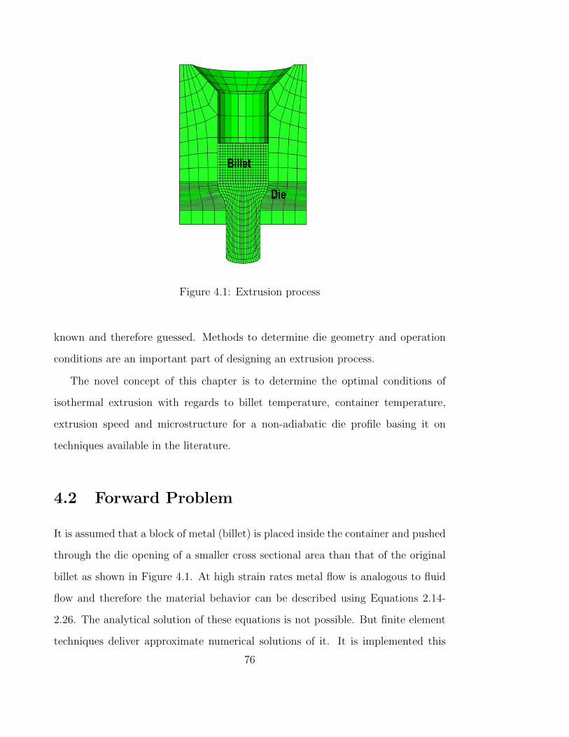
Figure 4.1: Extrusion process
known and therefore guessed. Methods to determine die geometry and operation
conditions are an important part of designing an extrusion process.
The novel concept of this chapter is to determine the optimal conditions of
isothermal extrusion with regards to billet temperature, container temperature,
extrusion speed and microstructure for a non-adiabatic die profile basing it on
techniques available in the literature.
4.2 Forward Problem
It is assumed that a block of metal (billet) is placed inside the container and pushed
through the die opening of a smaller cross sectional area than that of the original
billet as shown in Figure 4.1. At high strain rates metal flow is analogous to fluid
flow and therefore the material behavior can be described using Equations 2.14-
2.26. The analytical solution of these equations is not possible. But finite element
techniques deliver approximate numerical solutions of it. It is implemented this
76

with The ABAQUS finite element program.
4.3 Inverse Problem
The goal here is to determine the input data (parameters) of the forward problem
which leads to a given result. In this problem, the die design parameters and
process parameters are unknown, but the shape and properties of the final product
are known. It has been assumed here that the desired grain size of the material
is known, but the exact die geometry, initial billet temperature and ram speed
are unknown. Our aim is to estimate the exact die geometry and the process
parameters. This problem is known mathematically as an inverse problem and can
be seen as an optimization problem whereby the objective function to minimize is
the gap between the expected result and finite element simulation results.
First of all, a mathematical definition of the gap between the expected and
simulation results is required as an objective function. The aim of optimization is
to find the best set of parameters that minimizes an objective function by improving
the performance in the direction of optima. The aim of the approach is to find the
global minimum on a given search space by maximizing or minimizing the objective
function subjected to the given constraints. In the case of a minimization problem,
the mathematical formulation of the problem can be stated as follows
Minimize f(p)
subject to gj(p) ≥ 0 j = 1, . . . , n1
hk(p) = 0 k = 1, . . . , n2 (4.1)
where f(p) is the objective function, gj(p), hk(p) are constraints function and p is
a vector of design and process variables.
77

4.3.1 Design Variables
In order to determine the optimal die profile, it is essential to describe an arbitrary
die profile by a mathematical expression and obtain the design variables from the
expression. The design variables will then be optimized to get a desired result. In
this study Bezier curves with five control points are used to obtain the arbitrary
die profile. The Bezier curve which has the control points (xi, yi), i = 1, . . . , 5 is
given by [54]
x(t) =N∑i=0
xi+1Bi,N(t), and
y(t) =N∑i=0
yi+1Bi,N(t), (4.2)
where N = 4, t ∈ [0, 1], and
Bi,N(t) =N !
i!(N − 1)!ti(1− t)N−i
Using these control points, infinitely as many die surfaces can be created. Some
of these possible die surfaces are shown in Figure 4.2B. These are Bezier curves
obtained using its control points P1, P2, P3, P4 and P5. All these possible die
profiles are constructed by moving the control points P2, P3, P4 and P5 to all
possible positions. If point P2 coincides with P1 and P4 coincides with P5 then the
die profile becomes conical.
4.3.2 Process Variables
Theoretically, the process variables which can influence the extrusion process are
the ram speed VR, initial temperature of the billet TB0, initial die temperature TD0
and the friction conditions m at the billet/tool interface.
78
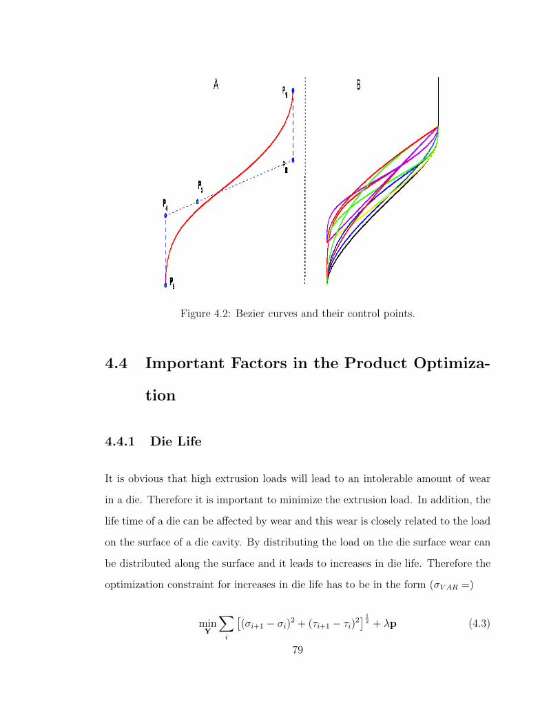
Figure 4.2: Bezier curves and their control points.
4.4 Important Factors in the Product Optimiza-
tion
4.4.1 Die Life
It is obvious that high extrusion loads will lead to an intolerable amount of wear
in a die. Therefore it is important to minimize the extrusion load. In addition, the
life time of a die can be affected by wear and this wear is closely related to the load
on the surface of a die cavity. By distributing the load on the die surface wear can
be distributed along the surface and it leads to increases in die life. Therefore the
optimization constraint for increases in die life has to be in the form (σV AR =)
minY
∑i
[(σi+1 − σi)2 + (τi+1 − τi)2
] 12 + λp (4.3)
79

where σi is the axial stress in the i−th node, τi is the friction stress in the i−th
node, p is the extrusion load, λ is a penalty parameter and Y, is a vector of
design and process parameters. Figure 4.3 and Figure 4.4 respectively give the
extrusion pressures and die pressure variations on the die surface with different die
geometries. Here the term die geometry number refers to the number of different
die shapes under consideration. The order of die geometry number depends on how
the control points of die geometry are arranged in a sequence. Figure 4.5 gives the
extrusion pressure and load distribution on the die surface. These graphs clearly
show the importance of the above optimization criteria and demonstrate how the
extrusion pressure and load on the die surface vary with the different die geometry.
These results further indicate that there is no die geometry which gives both lowest
extrusion pressures, die pressure and load variation on the die surface. Therefore a
trade off between these variables is necessary to find the optimum die geometry.
Figure 4.3: (A) Extrusion pressure variation [a: V0 = 6.3 mm/s, TD0 = 450oC,TB0 = 500oC, b: V0 = 25 mm/s, TD0 = 450oC, TB0 = 500oC, c: V0 = 25 mm/s,TD0 = 400oC, TB0 = 450oC.]
80

Figure 4.4: Die pressure variation with die geometry [a: V0 = 6.3 mm/s, TD0 =450oC, TB0 = 500oC, b: V0 = 25 mm/s, TD0 = 450oC, TB0 = 500oC, c: V0 =25 mm/s, TD0 = 400oC, TB0 = 450oC.]
Figure 4.5: Comparison of extrusion pressure and Load variation on die surfacewith die geometry [a: VR = 6.3 mm/s, TD0 = 450oC, TB0 = 500oC]
81

4.4.2 Isothermal Extrusion
Isothermal extrusion is a process of maintaining a constant temperature during
the extrusion process inside the deformation zone. Achieving this condition is
very important for the production of uniform, high-quality products. Isothermal
conditions can be achieved mechanically by adjusting the speed of the ram, initial
temperature of billets and die and by carefully designing the die for each product.
Several techniques can be used to achieve an isothermal extrusion process. These
can be divided mainly into three types: (1) Setting up a longitudinal thermal
gradient in the billet (tapered billet) before starting extrusion i.e the temperature
decreases faster in the front part of the billet than in the rear. (2) Maintaining
the extrudate exit temperature by varying the ram speed. (3) Maintaining the
extrudate exit temperature by varying the die shape. Although there are many
advantages that could be achieved, there are also some problems with regard to
isothermal extrusion. If the velocity gradient varies it could trigger a part to bend
or twist [57], thereby creating stresses and this is also applicable for variations in
temperature. Therefore it is important to adjust the material flows through the
die by changing the die shape. Based on these considerations the optimization
constraint to achieve isothermal extrusion can be written as follows.
minY
∫ tf
0
(T (x, y, t)− Td) dt, (4.4)
where T (x, y, t) is the temperature inside the deformation zone as a function of
space and time, Td is the average temperature or desired temperature inside the
deformation zone and tf is the time to complete the particular extrusion process.
The shape of the deformation zone and four points A, B, C and D inside the
zone are shown in Figure 4.6. The average temperature variation TV AR inside the
82
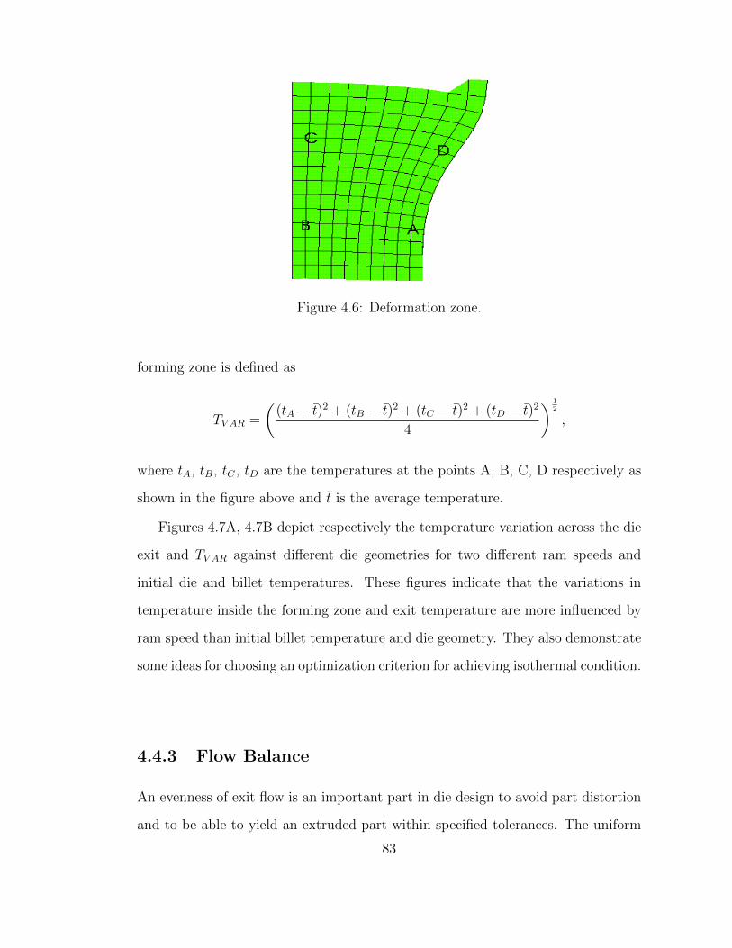
Figure 4.6: Deformation zone.
forming zone is defined as
TV AR =
((tA − t)2 + (tB − t)2 + (tC − t)2 + (tD − t)2
4
) 12
,
where tA, tB, tC , tD are the temperatures at the points A, B, C, D respectively as
shown in the figure above and t is the average temperature.
Figures 4.7A, 4.7B depict respectively the temperature variation across the die
exit and TV AR against different die geometries for two different ram speeds and
initial die and billet temperatures. These figures indicate that the variations in
temperature inside the forming zone and exit temperature are more influenced by
ram speed than initial billet temperature and die geometry. They also demonstrate
some ideas for choosing an optimization criterion for achieving isothermal condition.
4.4.3 Flow Balance
An evenness of exit flow is an important part in die design to avoid part distortion
and to be able to yield an extruded part within specified tolerances. The uniform
83

Figure 4.7: Comparison of (A) maximum temperature difference at the die exitand (B) TV AR with different die geometries, ram speeds and initial temperatures [a:v = 6.3 mm/s, TD0 = 450oC, TB0 = 500oC, b: v = 25 mm/s, TD0 = 450oC,TB0 = 500oC, c: v = 25 mm/s, TD0 = 400oC, TB0 = 450oC .]
die exit velocity can be obtained by adjusting the die land length. The optimization
constraint to increase the evenness of exit flow is therefore
minY
[N∑1
(Vi − V )2
], (4.5)
84

Figure 4.8: Flow balance: (A) Comparison with two different ram speeds, (B)Comparison with two different initial temperatures [ a:v = 6.3 mm/s, TD0 =450oC, TB0 = 500oC, b: v = 25 mm/s, TD0 = 450oC, TB0 = 500oC, c: v =25 mm/s, TD0 = 400oC, TB0 = 450oC.]
where Vi is the nodal velocity of the i−th node, N is the number of nodes along the
die exit and V is the average nodal velocity along the die exit. Figure 4.8 depicts
the exit velocity variation across the die exit against different die geometries for
different ram speeds and initial die billet temperatures. These figures indicate that
the variations in flow velocity across die exit are influenced by both ram speed,
85

initial billet temperature and die geometry. Further the velocity variations are more
sensitive to the die geometry than initial billet temperature and ram speed. These
results demonstrate that the problem of minimizing flow variation can be achieved
by altering die design parameters, ram speed and initial billet temperature.
4.4.4 Distortion
The success of an extrusion process depends mainly on reducing the distortion and
minimizing the redundant strain in the extruded product as well as controlling the
strain rate inside the deformation zone. Literature [37] in the field of metal forming
processes suggests that redundant strain and distortion are related to each other.
Based on the theory and available literature the following three criteria can be used
to minimize distortion.
(i) Distortion variation:
minY
[N∑1
(Ui − U)2)
](4.6)
where Ui is the displacement of the node i and U are the average displacements
of transverse nodes at the die exit.
(ii) Average effective strain:
minY
[N∑1
(εi − εIdeal)2)
](4.7)
where εIdeal is the ideal effective strain and is defined by
εIdeal = 2 lnR0
Rf
(4.8)
for axisymmetric extrusion.
86

Figure 4.9: Comparison of (A)Displacement variation, (B) Strain variation at thedie exit with different die geometries, ram speeds and initial temperatures[ a: v =6.3 mm/s, TD0 = 450, TB0 = 500, b: v = 25 mm/s, TD0 = 450oC, TB0 =500oC, c: v = 25 mm/s, TD0 = 400oC, TB0 = 450oC ].
(iii) Strain rate deviation:
minY
[N∑1
(εi − ¯ε)2)
](4.9)
Figure 4.9 depicts the average displacement variation and strain variation of the
transverse nodes across the die exit against different die geometries for different ram
speeds and initial die billet temperatures. Figure 4.10B and Figure 4.10C depict
the relative displacement of the nodes along the transverse lines with respect to
its original position and the strain values respectively. It can be seen clearly that
the strain increases from the centre line to the outer surface and is approximately
proportional to the displacement of the transverse nodes. If the strain values along
the transverse line are equal to the ideal effective strain (Equation 4.8) then there
would be no distortion at all.
Figure 4.11A depicts the comparison of average strain rate variation along the
transverse line at the die exit for different dies at two different ram speeds. Figure
87

Figure 4.10: (A) Nodes along transverse line, (B) Relative distortion, and (C)Effective strain distribution from the center line to the outer radius.
Figure 4.11: Strain rate variation at the die exit with die geometry: (A) Com-parison with two different ram speeds, (B) Comparison with two different initialtemperatures [ a:v = 6.3 mm/s, TD0 = 450oC, TB0 = 500oC, b: v = 25 mm/s,TD0 = 450oC, TB0 = 500oC, c: v = 25 mm/s, TD0 = 400oC, TB0 = 450oC .]
4.11B depicts the comparison of average strain rate for two different initial tem-
peratures. Figure 4.12 depicts the strain rate variation along the die neck for five
different die geometries. This shows clearly that the strain rate distribution of ge-
88
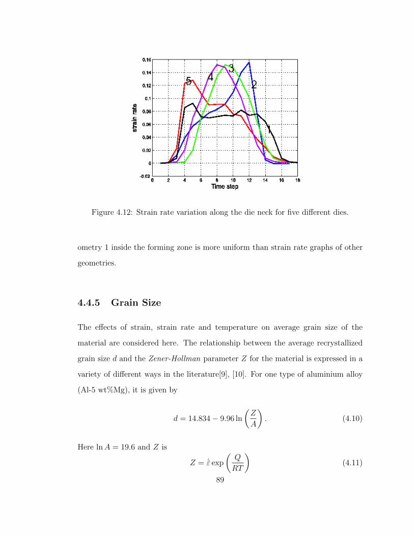
Figure 4.12: Strain rate variation along the die neck for five different dies.
ometry 1 inside the forming zone is more uniform than strain rate graphs of other
geometries.
4.4.5 Grain Size
The effects of strain, strain rate and temperature on average grain size of the
material are considered here. The relationship between the average recrystallized
grain size d and the Zener-Hollman parameter Z for the material is expressed in a
variety of different ways in the literature[9], [10]. For one type of aluminium alloy
(Al-5 wt%Mg), it is given by
d = 14.834− 9.96 ln
(Z
A
). (4.10)
Here lnA = 19.6 and Z is
Z = ˙ε exp
(Q
RT
)(4.11)
89

where A is a constant, Q is an activation energy and is about 135 kJ/mol, ˙ε is the
average strain rate, T is the temperature and R is the universal gas constant [66].
For AZ31 alloy it is given by [9]
ln d = 9.0− 0.27 lnZ. (4.12)
and for one type of steel it is given by [76]
d = 22600˙ε−0.27
exp
(−0.27
Q
RT
). (4.13)
All these equations are based on experimental observations and therefore the un-
certainty of constants are high. Further by using regression Equation (4.10) can be
written in the form of
d = 210˙ε−0.044
exp
(−0.044
Q
RT
). (4.14)
All these equations show that the grain size depends mostly on temperature and
strain rates. Therefore it is worthwhile to look at the changes of temperature
and strain rates at the die exit. Figures 4.13A and 4.13B depict respectively
the variation of temperature and strain rate and Figures 4.14A, 4.14B and 4.14C
respectively depict the variation of exp(0.044 QRT
) (say Y1), ε−0.044 (say Y2), and
ε−0.044 exp(−0.044 QRT
) (say Y3) across the die exit of die number 8 with two differ-
ent ram speeds and initial temperatures. These figures clearly demonstrate that
the variation in grain size can be minimized by minimizing the temperature and
strain rate variation across the die exit. The idea of these figures is to show how the
temperature, strain rate and grain size varies across the exit dependent on various
different extrusion speeds and initial temperatures.
90

Figure 4.13: Variation of (A) Strain rate and (B) Temperature along the die exitfor the die number 8 with different ram speeds and initial temperatures [a:v =6.3 mm/s, TD0 = 450oC, TB0 = 500oC, b: v = 25 mm/s, TD0 = 450oC,TB0 = 500oC, c: v = 25 mm/s, TD0 = 400oC, TB0 = 450oC.]
4.5 Objective and Constraint Function
The selection of the objective function is associated with the user’s specific needs.
Here the aim of this study is to extrude a product with given characteristics. There-
91

Figure 4.14: Comparison of grain size variation along the die exit for the die number8 with different ram speeds and initial temperatures:(A) Y1 = exp(−0.044 Q
RT), (B)
Y2 = ε−0.044, (C) Y3 = ε−0.044 exp(−0.044 QRT
)[ a:v = 6.3 mm/s, TD0 = 450oC,TB0 = 500oC, b: v = 25 mm/s, TD0 = 450oC, TB0 = 500oC, c: v = 25 mm/s,TD0 = 400oC, TB0 = 450oC.]
92

fore the objective function must involve the microstructure (grain size) of the final
product. The optimal strain rate, strain and temperature trajectories can be ob-
tained to get a desired value of grain size by minimizing [77]
J = W (ε(tf )− ε0) +
∫ tf
0
(d(t)− d0) (4.15)
where ε0 is a desired strain, W is a weighting factor, tf is the extrusion time, d0 is
a desired value of average grain size and the average grain size d is [77]
d = α
(˙ε exp
(Q
RT
))β. (4.16)
The objective function to determine the optimal die profile is the least square
deviation between the results obtained using Equation 4.15 and the finite element
solution of Equations 2.14-2.26. If the time interval [0, tm] is subdivided into m
partitions then the objective can be expressed by
λ1 minY
m+1∑1
(εi − εi)2 + λ2 minY
m+1∑1
(εi − ¯εi)2 + λ3 min
Y
m+1∑1
(Ti − Ti)2 (4.17)
Further if die life and flow balance are considered then the Equations 4.3 and 4.5
can be included as constraints with the objective function 4.17.
4.6 Schema of the Design
Let us now consider the technical design details of the algorithm to solve Equation
4.17. The solution will be arrived at through several steps as shown in Figure 4.15.
They consist of:
(i) The input data define the physical structure by its dimensions, material prop-
erties and boundary conditions.
93

Figure 4.15: Illustration of design process.
(ii) MATLAB’s lsqnonlin optimization algorithm is applied to obtain the optimal
values of strain-rate, strain values and temperature for given microstructure
properties of the material.
(iii) The input file module creates a model for the finite element analysis. It
consists of geometry of the model, material properties, contact definitions and
loading sequence etc. This is done with a MATLAB script which creates an
94

input file for the ABAQUS program. The reason for choosing this approach
is the possibility of easy modification of the die geometry for each iteration
process in the optimization routine.
(iv) FEM simulation part executes the created input file using ABAQUS explicit.
(v) The extraction module retrieves results from the ABAQUS ODB database.
Here the interface is set up between MATLAB ’s optimization procedure and
ABAQUS finite element simulation. This is achieved through the use of
PYTHON scripts to retrieve necessary results from the ABAQUS output
(ODB) database. It is saved in a different file with an EXCEL file format and
then processed with MATLAB to obtain the results for optimization.
(vi) The optimisation part is implemented using MATLAB ’s lsqnonlin built-in
function which uses the Levenberg-Marquardt algorithm. This approach en-
sures an easy implementation of multiple runs of ABAQUS within an opti-
mization routine.
Unlike the linear problem, the non-linear objective function given by Equation 4.17
may have more than one minimum. Therefore, the solution process should include
finding the global minimum. To deal with these problems first all or most of the
local minima of Equation 4.17 are found for a sequence of design variables at a
larger interval. Then the lowest value of the minima is picked. In the next step
the minimum obtained from the previous step is used as the starting value to solve
Equation 4.17.
4.7 Results and Discussion
In order to study the optimum results of an aluminium extrusion process, a FE-
simulation is carried out using MATLAB and ABAQUS. The process here is a
95

hot extrusion process with heat transfer between the work-piece and die being
considered. The work-piece and die have an initial temperature of T = 450oC. The
extrusion ratio is 1.33. The friction factor at the die-material interface is assumed
to be 0.1. The die is considered as a deformable body. Ram velocity is 6.25 mms−1.
The flow stress-strain relationship of the work-piece (aluminium alloy) material is
[83]
σ = 209 (ε)0.122 N/mm2 (4.18)
Other data values used in the simulation of the work-piece are: Young’s modulus of
E = 7×10¹⁰ Pa, coefficient of expansion= 8.4×10⁻⁵ oC−1 at T = 20 oC, Poisson’s
ratio= 0.35, inelastic heat fraction = 0.9, specific heat = 910 Jkg−1K−1, density=
2750 kgm−3, conductivity = 204 Wm−1K−1 when T = 0 oC, = 225 Wm−1K−1
when T = 300 oC and the values used for the die material are Young’s modulus of
E = 20×1010 Pa, coefficient of expansion= 8.4×10⁻⁵ oC−1 at T = 20 oC, Poisson’s
ratio= 0.30, inelastic heat fraction = 0.9, specific heat = 450 Jkg−1K−1, density=
7200 kgm−3, conductivity = 204 Wm−1K−1 when T = 0 oC, = 225 Wm−1K−1
when T = 300 oC.
First extrusion pressure, die pressure, temperature variation inside the defor-
mation zone, velocity variation at the die exit, distortion variation, strain variation
and strain rate variation at the die exit are minimized separately to study how
each property vary with the process and design parameters. It is interesting to find
that the optimal parameter values were not the same (eg. the parameters which
minimizes the extrusion pressure are not same as the parameters which minimizes
temperature variation inside the die) for all categories.
Secondly the circumferential, axial stress and hydrostatic pressure at the die
exit are compared. The contour plot of circumferential stress, axial stress and
hydrostatic pressure at the die entrance for three different dies (A: which needs
minimum extrusion pressure, B: which minimizes the velocity variation at the exit,
96

Figure 4.16: Circumferential stress (Pa) when :(A) Extrusion pressure, (B) Velocityvariation at exit, (C) Strain-rate variation at exit are lowest.
Figure 4.17: Axial stress (Pa) when :(A) Extrusion pressure, (B) Velocity variationat exit, (C) Strain-rate variation at exit are lowest.
C: which minimizes strain rate variation), are shown respectively in Figure 4.16,
4.17 and 4.18. It has been found, that the die, which minimizes the strain rate
variation at the exit also produces the profile with lowest circumferential stress and
the die, which minimizes the extrusion pressure, produces the profile with minimum
axial stress, which can be expected. The review of literature [67] showed, that the
97

possibility of cracking increases with increasing tensile circumferential stresses and
chevron(or central) bursts increase with increasing axial stress. Therefore it is
important and necessary to include the minimization of circumferential and axial
stress during the optimization process.
The tendency toward chevron cracking increases, if plastic zones do not meet
together inside the forming zone. The probability of chevron cracking increases
with decreasing extrusion ratio. If this happens the hydrostatic pressure at that
region is zero. It can be shown that the hydrostatic pressure is not zero inside
the forming zone for any of the above mentioned cases (which minimizes extrusion
pressure, die pressure, temperature variation, and strain rate variation etc) and in
certain non optimal cases as shown in Figure 4.19 (eg. when extrusion pressure is
maximum) the hydrostatic pressure inside the forming zone is zero.
The average grain size is proportional to
d
α=
(˙ε exp
(Q
RT
))β. (4.19)
Here d is an average grain size and α is a constant. The variation of the four most
optimized d/α values along the die exit with different process conditions are shown
in Figure 4.20. Most optimal (in terms of uniformity) d/α values of four different
cases and their respective die surface which gives the optimum are shown in Figure
4.21. These figures clearly show that the grain size is more sensitive to extrusion
speed and the initial temperature than the die geometry. Further the uniformity
of the grain size is more influenced by the shape of the die surface than initial
temperature or ram speed. Therefore, a certain grain size with uniformity could be
achieved by trading off between these parameters.
Finally the grain size variation with various desired grain sizes for a sequence
of design and process parameters are considered and it is found that values of
98

Figure 4.18: Hydrostatic pressure (Pa) when :(A) Extrusion pressure, (B) Velocityvariation at exit, (C) Strain-rate variation at exit are lowest.
parameters (design and process) exist to satisfy equations 4.6– 4.9.
Figure 4.19: Hydrostatic pressure (A) inside the forming zone, (B) along the Path1 .
4.8 Summary
The goal of the work presented here is to investigate a numerical technique which
is capable of simultaneously estimating the optimal die profile and the process
99

Figure 4.20: Grain size variation along the die exit (d/α) (A) when v = 6.3 mm/s,TD0 = 450oC, TB0 = 500oC, (B) when v = 25 mm/s, TD0 = 450oC, TB0 = 500oC,(C) when v = 25 mm/s, TD0 = 400oC, TB0 = 450oC.
parameters such as extrusion speed and initial temperatures. The approach is
based on a non-linear least squares estimation using the desired properties of the
product which is extruded.
The examples considered in the above section describe how values of the design
and process parameters influence the optimization process. The results from these
examples suggest that the proposed technique is capable of estimating the optimal
values well.
100

Figure 4.21: Grain size variation along the die exit (d/α):(A) Optimal vales withdifferent process conditions, (B) Optimal die shape with different process conditions.
101

102

Chapter 5
Estimation of Average Grain Size
and Material Constants
5.1 Introduction
Numerical modelling of extrusion may be used during a design process to assess the
extruded material properties. The extrusion simulation describes the material flow
through the die. An extrusion model, which is capable of describing the behaviour
of material flow, requires the following input data: (a) material data such as Young’s
modulus, coefficient of expansion, Poisson’s ratio, inelastic heat fraction, specific
heat, density, conductivity, flow stress-strain relationship, (b) die design variables
and (c) process variables such as ram speed, initial temperature and friction factors.
In reality, material data can be measured using available measuring instru-
ments, but the optimal values of die design variables and process variables are
often unknown. In the previous chapters, a non-linear least squares inverse model
is formulated in which the optimal values of die design variables and process vari-
ables were estimated to achieve a certain grain size. In this approach the following
103

average grain size equation [76], [77]
d = α
(dε
dtexp
(Q
RT
))β(5.1)
was used as optimizing criteria to terminate the problem. In equation 5.1, Q is an
activation energy, d is the average recrystallized grain size, T is the temperature,
dε
dtis the strain rate and R is the universal gas constant.
The values of constants α and β are based on experimental observations and
therefore the uncertainty of the constants can be very high. Small changes in these
values can cause variation in the grain size estimation. The successful application of
equation (5.1) depends on the accuracy of the parameters. Methods to identify the
optimal values of α and β are therefore an important part of modelling extrusion
processes to increase the reliability of the numerical simulation.
In this chapter an alternative method is proposed. The idea is to develop an
inverse model for estimating grain size history, using inverse modelling techniques
available in the literature. Inverse modelling avoids the use of α and β for the grain
size history estimation. To do so the problem in which the material properties of
the billet as well as process and die design parameters are known but the material
constants α, β and grain size d are not known is considered. The accuracy of the
model is examined by using simulated temperature and strain data (generated by
the forward model) to which normally-distributed relative noise has been added.
The inverse model is designed as a least squares minimisation problem associated
with an ABAQUS finite element solution of an extrusion process. This is an ill-
posed problem and it is solved using regularisation methods.
104

5.2 Forward Problem
The thermo-mechanical behaviour of the extrusion process can be described math-
ematically using equations (2.14-2.26). The solutions can be obtained with finite
element methods. The solution procedure is implemented using ABAQUS to ob-
tain temperature and strain histories during the deformation process. Once the
temperature and strain values are obtained, the average grain size at a nodal point
can be calculated with equation 5.1.
5.3 Inverse Problem
The goal of inverse modelling is the extraction of model parameter information
from data. It is a subject, which supplies tools for the proficient use of data in
the estimation of constants appearing in the models. In this inverse problem, the
structure of the equation is known; outputs, temperature (T ) and strain (ε) values
are available. Average grain size history and parameters α and β are the unknowns.
In this section a model is formulated to obtain the best estimate of grain size
history, α and β appearing in equation 5.1 from temperature and strain estimations
made at some nodes in the material inside the forming zone. The microstructural
model given by equation (5.1) can be rewritten to solve for strain rate as follows.
dε
dt=
(d
α
)1/β
exp
(−QRT
)(5.2)
Therefore the strain is
ε(t) =
∫ t
0
(d(τ)
α
)1/β
exp
(−QRT (τ)
)dτ
=
∫ t
0
K(t, τ)D(τ)dτ (5.3)
105

where the kernel K(t, τ) is:
K(t, τ) = exp
(−QRT (τ)
)(5.4)
and
D(τ) =
(d(τ)
α
) 1β
(5.5)
If n temperature and strain values are available at the node (X1, Y1, Z1) between 0
and tf and supposing that D(τ) at times τ0 = 0, . . ., tf are to be determined, then
discretising (5.3) by the trapezoidal rule gives a system of linear equations
e = A(p)q (5.6)
where e = [ε(0), . . . , ε(tf )]T, Aij = K(ti, τj)βij, q = [D(τ0), . . . , D(τf )]
T and p =
[Q], and βij is a quadrature weight. Generally, minimising an objective function
solves inverse problems. The objective function Z that provides minimum variance
estimates is the ordinary least squares function
minimize Z (p, q) = ‖A(p)q− e‖22 (5.7)
If the value of activation energy Q is known then the problem becomes a linear least
square problem and can be solved easily. But the coefficient matrix of problem 5.7
always has a very large condition number and is ill posed. Therefore well posed
situation must be restored by restricting the class of admissible solutions. This can
be achieved using regularisation methods [29]. With Tikhonov’s regularisation, the
regularised objective function
Z (q) = ‖Aq− e‖22 + λ2‖Lq‖2
2 (5.8)
106

is introduced where ‖Aq − e‖22 is the residual norm (or data misfit function), and
‖Lq‖22 is the solution norm. The minimisation of the function Z(q) for different
values of λ will be interested. Note that the objective function Z is the 2-norm of
the following system of equations
A
λL
q =
e
0
,where L is the regularisation operator and is defined by
‖Lq‖2 =
∫ t
0
(dNq
dτN
)2
dτ, (5.9)
and λ is the regularisation parameter. The regularisation parameter λ has to be
altered in such a way that the solution fits well in some optimal way.
If the value of Q is not known then the problem becomes a nonlinear least square
problem as follows.
Z (q, p) = ‖A(p)q− e‖22 + λ2‖Lq‖2
2. (5.10)
Since the equation (5.10) has a combination of linear parameters q and non-linear
parameters p, the solution process is separated into two steps. The non-linear
parameter p is found by constructing an iterative procedure, where at each iteration
a linear sub-problem is solved to estimate the linear parameter q corresponding to
that particular value of p.
Now taking natural logarithms of both sides of the equation 5.5 and rearranging
gives
ln(D) = m ln(d) + C (5.11)
where m =1
βand C =
1
βln
(1
α
). Now supposing n+ 1 D values are available the
107

corresponding d values are to be determined. This gives
Ky = f , (5.12)
where
K =
m 0 . . . 0 0
0 m . . . 0 0
......
......
...
0 0 . . . m 0
0 0 . . . 0 m
y =
ln(d1
d0
)ln(d2
d0
)...
ln(dn−1
d0
)ln(dnd0
)
, f =
ln(D1
D0
)ln(D2
D0
)...
ln(Dn−1
D0
)ln(DnD0
)
Now the minimisation problem for estimating y is formulated as
miny‖Ky − f‖2
2. (5.13)
It is a linear problem and therefore the grain size history d1, d2, . . . , dn can be
calculated with reasonable accuracy provided the initial grain size is known.
5.4 Applications
In this section, numerical simulations to demonstrate the solution process are pre-
sented and the accuracy of the model is evaluated. To do so, an input of tem-
perature and strain value data generated are considered at three elements A, B,
108

Figure 5.1: Three considered elements of a deformed mesh
C as shown in Figure 5.1 from a FE-simulation of extrusion using ABAQUS.
The data values used in the simulation of extrusion are: initial temperature of
work piece and die respectively are T = 500oC and T = 450oC, work piece’s
Young’s modulus E = 7 × 10¹⁰ Pa, coefficient of expansion 8.4 × 10⁻⁵ oC−1
at T = 20 oC, Poisson’s ratio 0.35, inelastic heat fraction 0.9, specific heat
910 Jkg−1K−1, density= 2750 kgm−3, conductivity 204 Wm−1K−1 when T = 0 oC,
225Wm−1K−1 when T = 300 oC, die material’s Young’s modulus E = 20×1010 Pa,
coefficient of expansion 8.4×10⁻⁵ oC−1 at T = 20 oC, Poisson’s ratio 0.30, inelastic
heat fraction 0.9, specific heat 450 Jkg−1K−1, density 7200 kgm−3, conductivity
204 Wm−1K−1 when T = 0 oC, 225 Wm−1K−1 when T = 300 oC.
109

Figure 5.2: (A):Total error, (B) L-curve.
5.4.1 Estimation of Grain Size d(t) for Known Value of Ac-
tivation Energy Q
If the value of Q is known, the Equation 5.8 has to be solved to estimate the
grain size. The minimization problem given by Equation 5.8 depends on the op-
timal value of the regularization parameter λ. A number of techniques have been
discussed in the literature[30] for estimating an optimal value of a regularization
parameter. Here the L-curve criterion is used to estimate the parameter values. It
is based on minimizing the total error equation 5.8 as shown in Figure 5.2. A good
regularization parameter λ should provide a fair balance between data misfit error
and regularization error. The L-curve method shown in Figure 5.2B is based on
minimizing total error as shown in Figure 5.2A.
Once the optimal value of λ is known, q = [D(τ0), . . . , D(τf )]T are easily es-
timated and then using equation 5.13 values y =[D1
D0, . . . , Dn
D0
]Tare calculated.
110
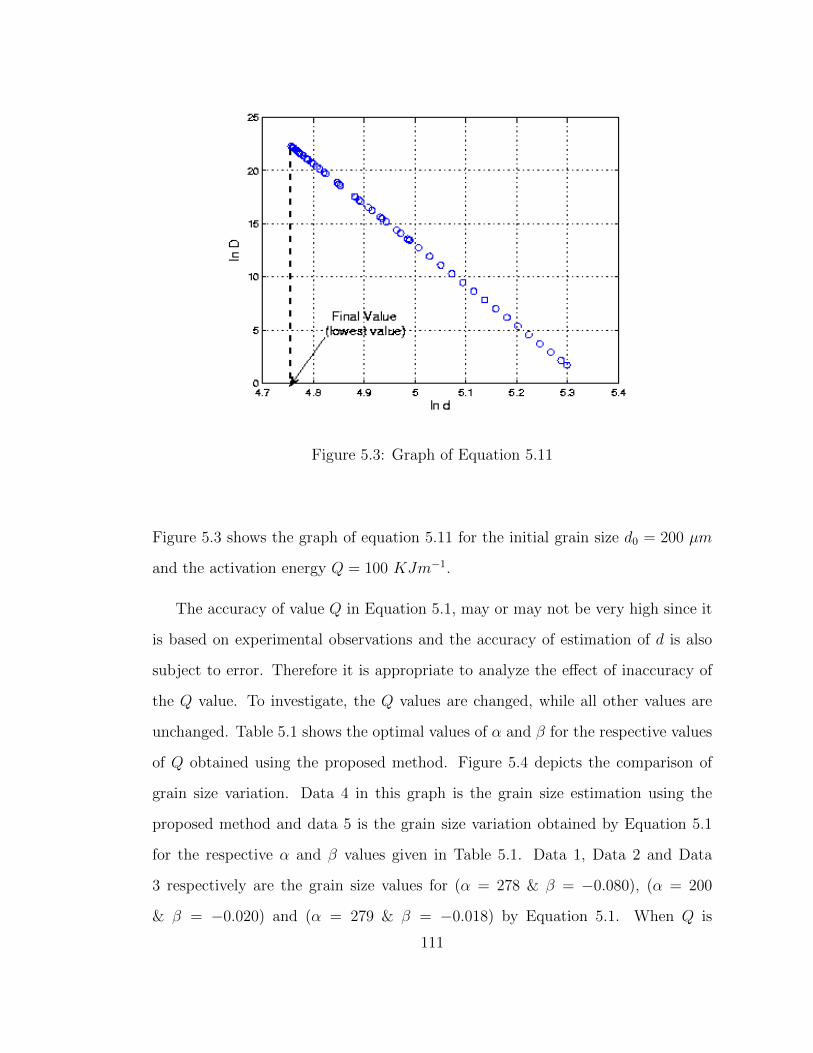
Figure 5.3: Graph of Equation 5.11
Figure 5.3 shows the graph of equation 5.11 for the initial grain size d0 = 200 µm
and the activation energy Q = 100 KJm−1.
The accuracy of value Q in Equation 5.1, may or may not be very high since it
is based on experimental observations and the accuracy of estimation of d is also
subject to error. Therefore it is appropriate to analyze the effect of inaccuracy of
the Q value. To investigate, the Q values are changed, while all other values are
unchanged. Table 5.1 shows the optimal values of α and β for the respective values
of Q obtained using the proposed method. Figure 5.4 depicts the comparison of
grain size variation. Data 4 in this graph is the grain size estimation using the
proposed method and data 5 is the grain size variation obtained by Equation 5.1
for the respective α and β values given in Table 5.1. Data 1, Data 2 and Data
3 respectively are the grain size values for (α = 278 & β = −0.080), (α = 200
& β = −0.020) and (α = 279 & β = −0.018) by Equation 5.1. When Q is
111

Q α βData1 20 140 -0.044Data2 50 278 -0.080Data3 100 209 -0.026Data4 140 200 -0.020Data5 180 240 -0.019Data6 220 279 -0.018Data7 300 412 -0.019
Table 5.1: Variation of α and β with Q values
Figure 5.4: Grain size vs activation energy for different material constants
underestimated, the average grain size estimated value using Equation 5.1 is higher
than it used to be and increases approximately quadratically with decreasing Q
value. When Q is overestimated, the average grain size estimated value is lower
than it used to be and decreases approximately quadratically with increasing Q
value. The graph of Data 4 and Data 5 are approximately the same. This shows
that even if the Q value is wrong, it is possible to estimate d accurately using
112

Equation 5.1 if appropriate α and β values are available. These results can’t be
gained by practical experiments, but can only be achieved through inverse modelling
techniques.
5.4.2 Estimation of d(t) for Unknown Value of Activation
Energy
Here the problem is concerned with the estimation of grain size d(t) values and
the activation energy (Q). This estimation process contains a combination of a
nonlinear parameter (Q) and linear parameters (d(t)). This is different from a
linear problem and therefore linear algebra cannot be used to solve this problem.
This problem can be solved by constructing an iterative procedure as mentioned
above. Alternatively the Equation 5.10 can be solved for a sequence of Q values
to get a best value for Q which minimizes Equation 5.10, since there is only one
nonlinear parameter. Figures 5.5A, 5.5B respectively show the variation of Z with
Q at the nodes A (data 1), B (data 2), C (data 3) for the ram speed 12.5 mm s−1
and 6.5 mm s−1. The graphs clearly show that the best value of Q is not the same
for all cases. In the literature it can be found that the activation energy of the
material varies with temperature. During the extrusion process the temperature
inside the deformation zone is not constant everywhere. Therefore using a constant
Q value in Equation 5.1 will not give an accurate result unless appropriate values
of α and β are used. Again the estimation of α and β which suits the Q value is
not achievable in a real practical environment.
113

Figure 5.5: Objective function Z vs Activation energy Q
5.5 Summary and Conclusion
The objective of the work demonstrated in this chapter is to develop an inverse
model capable of concurrently estimating the average grain size, activation energy
and other material constants appearing in the model. The approach is based on a
non-linear least squares estimation using simulated temperature and strain value
history inside the deformation zone. Since the problem is ill-posed, Tikhonov’s
regularisation method is applied to stabilise the solution process. Some of the pa-
rameters in the problem are linear and some are nonlinear. The linear parameters
are determined using simple linear algebra and for the computation of non-linear
parameters MATLAB ’s routine lsqnonlin is used. The optimal value of the regular-
isation parameter is obtained using the linear L-curve for the linear problem.
To summarize three points can be made: Firstly, the usefulness of an inverse
modeling technique in the grain size estimation process has been demonstrated. The
114
inverse modelling technique has been applied to Equation 5.1 with the situation in
which α, β and Q values are unknown. Secondly, it has been shown that the error
in traditional d estimation increases quadratically with the error in Q if the α and
β values are adjusted accordingly to cater for Q. The appropriate values of α
and β can only be found using the above mentioned inverse modelling technique.
Thirdly, it has been demonstrated the optimal value of the activation energy inside
the deformation region is not constant and varies with the temperature. Therefore
the traditional d estimation using Equation 5.1 with constant values of Q, α and β
will not give the accurate value, if the temperature inside the deformation zone is
not constant.
115

116

Chapter 6
Optimization of Pocket Design to
Produce a Thin Shape Complex
Profile
6.1 Introduction
The surface qualities of extruded products depend on process and die design pa-
rameters. In order to produce appropriate shapes with good surface quality and
homogenous structure the metal flow through the die should be as uniform as possi-
ble. Therefore the estimation of an optimal set of process and die design parameters
for a particular product geometry is an important part of an extrusion process.
The geometry of the product considered for the investigation is a current pro-
duction part. The profile geometry is shown in Figure 6.1. Since it is symmetry
about the axis and therefore only half of the part is considered as shown in Figure
6.1 is considered. This specific die geometry was selected because the extruded
product showed surface quality problems. After anodizing it has white lines along
the extrusion direction that make an uneven visual surface. These lines tend to
117

appear at different places on different production runs. They seem to be random in
whether they appear or not and when they do, it could be anywhere on the profile.
These lines are seen as flow–lines.
Flow–lines are distinctive surface marks and tangential to the machine direction.
They are very irregular in size, shape and position. According to the available
literature it is a region of highest shear stress. A poor temperature and velocity
uniformity inside the forming zone leads to a change in flow characteristics and
layer distribution.
Figures 6.3 and 6.4 depict the velocity, temperature and shear stress distribu-
tion of the extruded product between the entrance and exit of a die for the given
geometry. It shows that the temperature and velocity distributions are not ho-
mogenous. Further the location of the higher stress area was found moving with
different initial billet temperatures. All these results demonstrate the importance
to improve the die design. If the profile geometry is simple then the flow can be
adjusted by using a curved die. But here the profile geometry is complex and the
die is flat. There are several methods available to alter metal flow and temperature
distribution through a flat die. More reliable methods are (1) assigning a different
bearing length at different locations and (2) inclusion of a pocket (or pre-chamber)
in front of the die bearing. Even though the variation of the bearing length at
different locations is an effective method to control the metal flow the tendency
for extruded surface defects to occur will increase since more heat generates from
friction in certain regions of the interaction between billet and die bearing.
6.2 Finite Element Model
The finite element program DEFORM 3D is used in this analysis to simulate the
extrusion process as shown in Figure 6.5. It is based on the Lagrangian method and
118
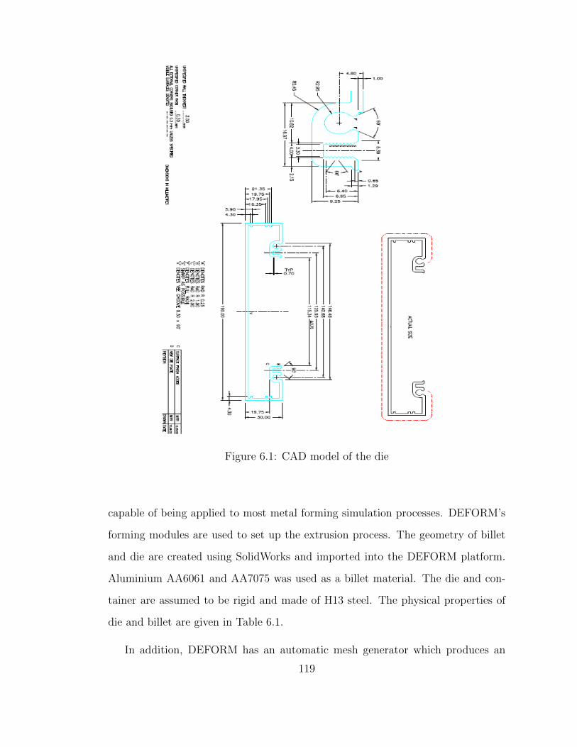
Figure 6.1: CAD model of the die
capable of being applied to most metal forming simulation processes. DEFORM’s
forming modules are used to set up the extrusion process. The geometry of billet
and die are created using SolidWorks and imported into the DEFORM platform.
Aluminium AA6061 and AA7075 was used as a billet material. The die and con-
tainer are assumed to be rigid and made of H13 steel. The physical properties of
die and billet are given in Table 6.1.
In addition, DEFORM has an automatic mesh generator which produces an
119

Figure 6.2: Geometry of the die
Material AA6061 AA7075 H 13propertiesHeat N/mm2 C 2.4 2.39 5.6capacityThermal W/m C 166 130 28.4conductivityHeat transfer N/ Csmm2 11 11 11coefficient betweendie and billetEmissivity 0.1 0.1 0.7
Table 6.1: Material properties of billet and die
optimized mesh with local element size control. More elements are used where
there are large deformations and fewer elements are used where little deformation
takes place.
In this study of simulation of extrusion, Coulomb friction is used when contact
occurs between billet and die. The frictional force in the Coulomb law model is
defined by
fs = µp
where fs is the frictional stress, p is the interface pressure between two bodies
and µ is the friction factor. A friction factor of 0.1 was used for most simulations
120
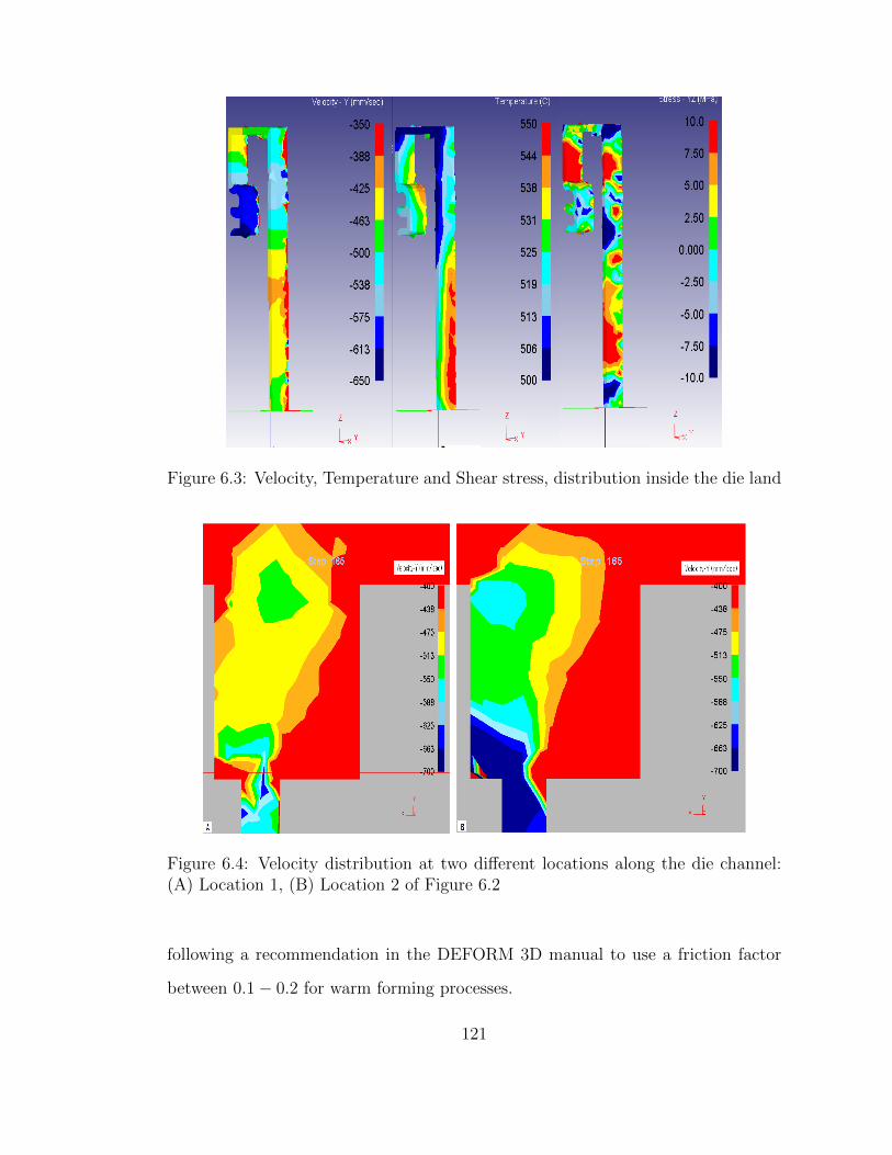
Figure 6.3: Velocity, Temperature and Shear stress, distribution inside the die land
Figure 6.4: Velocity distribution at two different locations along the die channel:(A) Location 1, (B) Location 2 of Figure 6.2
following a recommendation in the DEFORM 3D manual to use a friction factor
between 0.1− 0.2 for warm forming processes.
121

Figure 6.5: Finite element model
6.3 Analysis of the Influence of Pocket Design
Parameters
The surface finish of the extruded product is related to the flow pattern. The flow
pattern depends on pocket design parameters such as the pocket shape, the distance
between the centre axis of the die and centre axis of the pocket (rp), pocket depth
(d) and pocket width (w). In this section the influences of these parameters on the
flow pattern were investigated using a simple rectangular pocket die as in Figure
6.6.
6.3.1 Influence of Distance from Die Centre rp
Figure 6.7 shows the homogeneity of flow when the die channel is not in the middle
of the die axis (rP > 0). It can be seen from this figure that the flow through
the die channel is more homogeneous when the width of the pocket closer to the
122
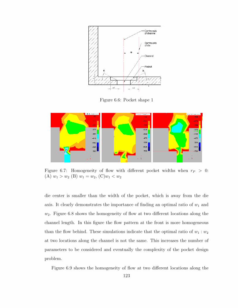
Figure 6.6: Pocket shape 1
Figure 6.7: Homogeneity of flow with different pocket widths when rP > 0:(A) w1 > w2 (B) w1 = w2, (C)w1 < w2
die center is smaller than the width of the pocket, which is away from the die
axis. It clearly demonstrates the importance of finding an optimal ratio of w1 and
w2. Figure 6.8 shows the homogeneity of flow at two different locations along the
channel length. In this figure the flow pattern at the front is more homogeneous
than the flow behind. These simulations indicate that the optimal ratio of w1 : w2
at two locations along the channel is not the same. This increases the number of
parameters to be considered and eventually the complexity of the pocket design
problem.
Figure 6.9 shows the homogeneity of flow at two different locations along the
123
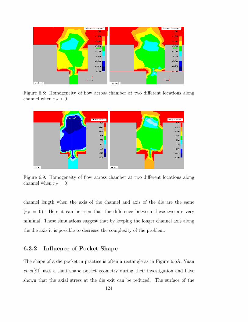
Figure 6.8: Homogeneity of flow across chamber at two different locations alongchannel when rP > 0
Figure 6.9: Homogeneity of flow across chamber at two different locations alongchannel when rP = 0
channel length when the axis of the channel and axis of the die are the same
(rP = 0). Here it can be seen that the difference between these two are very
minimal. These simulations suggest that by keeping the longer channel axis along
the die axis it is possible to decrease the complexity of the problem.
6.3.2 Influence of Pocket Shape
The shape of a die pocket in practice is often a rectangle as in Figure 6.6A. Yuan
et al [81] uses a slant shape pocket geometry during their investigation and have
shown that the axial stress at the die exit can be reduced. The surface of the
124

Figure 6.10: Homogeneity of flow with pocket shape: (A) rectangle,(B) slant,(C)curved
pocket can also be constructed using a series of Bezier curves. Figure 6.10 shows
the homogeneity of flow for the same condition but with three different types of
die. As can be seen from this figure, the homogeneity of flow with a slant pocket
die is much better than a rectangular pocket die. The homogeneity of flow is even
better in a Bezier curved die than a slant die.
6.3.3 Influence of Pocket Angle
It has been shown in the literature [44], [45] that there is an inverse linear relation-
ship between pocket angle and flow velocity when√d2 + w2 is constant. Here it
has been assumed that w1 = w2 = w. It is not possible to make a die pocket with
constant√d2 + w2 along the length of the die channel unless the bearing length of
the channel is allowed to vary along the length. Die bearing variation along the die
channel may increase the tendency of surface defects at certain regions where more
heat is generated from friction. In addition this will reduce the die life as well.
Therefore the die bearing length was not varied along the length. There is only
the option to change d and w subject to w2+d2 being not constant. In order to study
the effect of metal flow with different d and w values, two axis symmetry simple
geometry dies with extrusion ratio 10 were considered as in Figure 6.11. DEFORM
125

3D was used to simulate the extrusion process. The billet material used for the
investigation is Al 7575 and loaded from the DEFORM 3D database. The initial
temperature of die and billet respectively are 350oC and 400oC. The ram speed
is set as 50 mm/s. The friction coefficient is set as constant and values between
0.1 − 0.4 have been used for various simulations. Simulations were repeated for
various different entry angles and friction coefficients.
The velocity variation with pocket angle for a rectangular pocket and a slant
pocket respectively are plotted in Figures 6.12A and 6.12B. As can be seen from
Figure 6.12, the velocity is not linearly increasing or decreasing. In Figure 6.12B,
simulation results of velocity for a slant pocket are shown for various coefficients of
friction values. When the die angle increases flow will also increase but on the other
hand a changing surface area will influence the flow due to the friction between die
and work-piece. This surface area depends on the formation of dead metal zone
for the rectangle pocket die. There won’t be any dead metal zone for the slant
pocket die and hence the increase of frictional contact area will be proportional to
the angle. This is why it can be clearly seen that there is approximately a linear
relationship between the pocket angle and corresponding velocity when the design
of the pocket is slant.
6.3.4 Influence of Channel Length
In the literature [22] it has been mentioned that if the channel length is signifi-
cantly long, it will result in an essential difference of flow speeds along the channel
length. To investigate this effect a die as in Figure 6.13 was considered and then
the extrusion flow was simulated without any pockets. The billet material used for
the investigation is Al 7575, initial temperature of die and billet respectively are
400oC and 450oC, ram speed is set as 50 mm/s, and the friction coefficient is 0.1.
The extrusion speed at the die exit along the channel is plotted in Figure 6.16.
126

Figure 6.11: Layout of pocket geometry: (A) rectangular pocket, (B) slant pocket
Figure 6.12: (A) Rectangular pocket, (B) Slant pocket
As can be seen from this figure (line data 1–old die), the velocity along the channel
length tends to vary when the channel is reasonably long. This might be because
the metal away from the die axis tend to flow more slowly as a result of a billet-die
interface friction.
127

Figure 6.13: Sample die with extrusion ratio 1:51
6.4 Proposed Optimization Algorithms
From our investigation it has been found that (1) if the length of the channel is
large, it results in a great difference of flow speed along the length of channel; (2)
if the width ratio of the pocket at each side of a channel is not optimum, it will
result in a non homogeneous velocity distribution across the die width. Further the
width closer to the axis should be smaller than the width which is away from the
die axis. If the channel is symmetrical about the die axis, an equal pocket width at
each side will lead to a homogeneous velocity distribution across the width along
the channel.
The novel concept of this research is to determine the optimal geometry of
the pocket to achieve homogenous metal flow in terms of speed, temperature and
shear stress distribution inside the forming zone to extrude a product with the
geometry given in Figure 6.2. To deal with these problems two algorithms have
been developed to determine the best geometry of the pocket.
6.4.1 Algorithm -1
The solution is arrived at through three steps. In the first step, the channel was
divided into n elements as shown in Figure 6.13 and the flow velocity across each
128
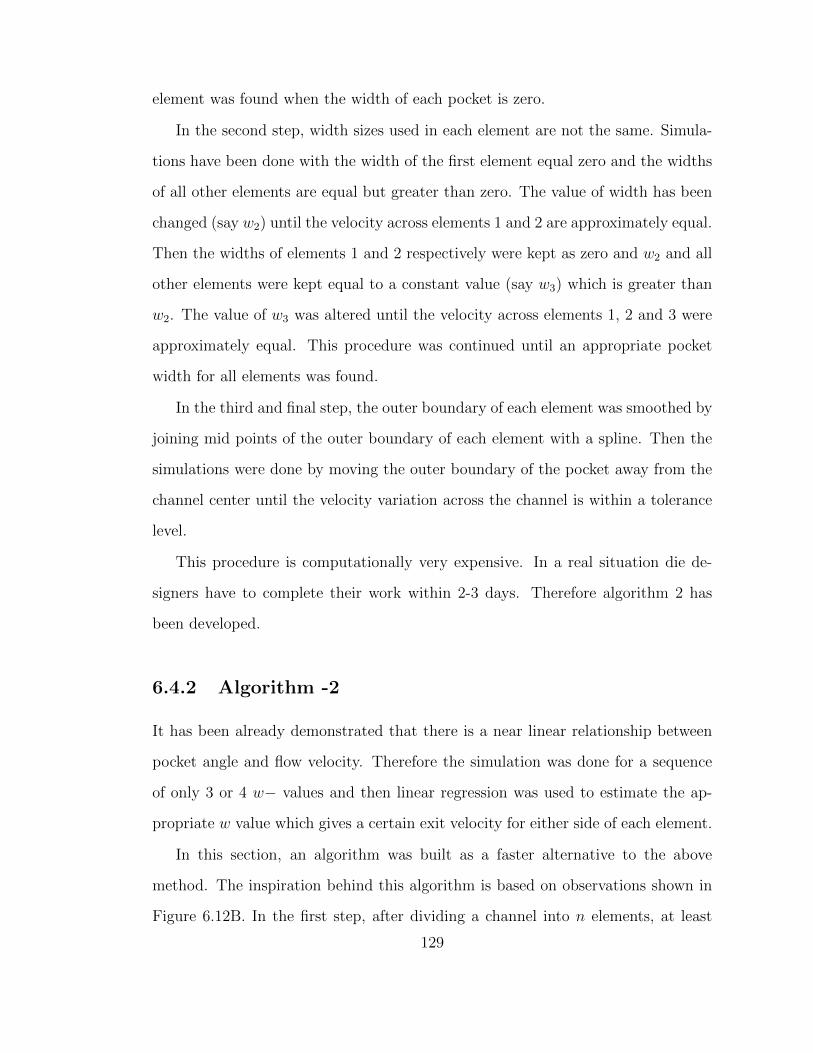
element was found when the width of each pocket is zero.
In the second step, width sizes used in each element are not the same. Simula-
tions have been done with the width of the first element equal zero and the widths
of all other elements are equal but greater than zero. The value of width has been
changed (say w2) until the velocity across elements 1 and 2 are approximately equal.
Then the widths of elements 1 and 2 respectively were kept as zero and w2 and all
other elements were kept equal to a constant value (say w3) which is greater than
w2. The value of w3 was altered until the velocity across elements 1, 2 and 3 were
approximately equal. This procedure was continued until an appropriate pocket
width for all elements was found.
In the third and final step, the outer boundary of each element was smoothed by
joining mid points of the outer boundary of each element with a spline. Then the
simulations were done by moving the outer boundary of the pocket away from the
channel center until the velocity variation across the channel is within a tolerance
level.
This procedure is computationally very expensive. In a real situation die de-
signers have to complete their work within 2-3 days. Therefore algorithm 2 has
been developed.
6.4.2 Algorithm -2
It has been already demonstrated that there is a near linear relationship between
pocket angle and flow velocity. Therefore the simulation was done for a sequence
of only 3 or 4 w− values and then linear regression was used to estimate the ap-
propriate w value which gives a certain exit velocity for either side of each element.
In this section, an algorithm was built as a faster alternative to the above
method. The inspiration behind this algorithm is based on observations shown in
Figure 6.12B. In the first step, after dividing a channel into n elements, at least
129

Figure 6.14: Velocity variation with angle θ
three simulations were done with different pocket widths but every element has
equal width value and the flow velocity across each element was noted.
In the second step, each element’s velocity is changed with w (or θ) which is
obtained from the first step to calculate m and C of equation v = mθ+C by using
linear regression as in Figure 6.14. Then for each element respective θ values have
been picked for which their velocity is equal to the velocity of the first element.
In the third step, the outer boundary of a pocket was formed by joining mid
points of the outer boundary of each element for the respective θ (or w) values with
a spline. This process was repeated (step 2 and 3) for various different velocities of
the first element until the velocity variation along the channel is minimum. Two
of many choices are shown in Figure 6.14 as first choice as well a next choice and
their pocket geometries are shown in Figure 6.15.
The shape of the orifices of both dies (selection 1 and 2) are exactly the same
130

Figure 6.15: Pocket geometries for first and next choice
Figure 6.16: Velocity distribution of the extrudate through original die, optimalpocket die and die with no pocket: data 1- old die, data 2- without pocket, data 3-optimal die
131

Figure 6.17: Relative comparison of velocity variation along the die channel withoptimal pocket geometry for different process conditions (v = 25, 50 and T =400oC, 450oC)
but the pocket area of selection 2 is larger than that of selection 1. This is especially
obvious at the half symmetry line of the dies. The pocket width of die 1 (selection
1) at the half symmetry line is zero and the width of die 2 (selection 2) at the half
symmetry line has a certain dimension. The greater value for the width is a result
of minimising the velocity variation along the channel.
Figure 6.16 shows the velocity at just outside the die exit along the channel
length for the optimal die together with the die without pocket and the original
die.
A comparison of the relative variation for the optimal die geometry with different
process conditions are shown in Figure 6.17. In the figure data 1 is obtained when
the ram speed is 25 mm/s, the initial billet is 400oC, data 2 is obtained when the
ram speed is 50 mm/s, the initial billet is 400oC, and data 3 is obtained when the
132

ram speed is 25 mm/s, and the initial billet is 450oC. Based on these observations
it can be said that the initial temperature is slightly more sensitive to the geometry
than the ram speed, although the overall variation from the optimum value is small.
Figures 6.18-6.19 depict the velocity, temperature and shear stress distribution of
the extruded product of material AA7075 between the entrance and exit of an
optimal die for different initial temperatures. Figure 6.20 depicts the velocity,
temperature and shear stress for the material AA6061. These figures show that the
velocity distributions at the die exit is approximately constant and temperature
variation along the channel is very small compared to Figure 6.3. Shear stress just
inside the die exit is also reduced. These figures also demonstrate an optimal die
is invariant to material variations. The optimal die geometry is shown in Figure
6.21A. For the comparison purposes the original die geometry also shown in Figure
6.21B. There are number of differences between the original pocket geometry and
optimal pocket geometry. It can be seen very clearly seen in the figure. Firstly the
optimal die pocket walls are not vertical. Secondly the pocket cross sectional area
increases from die centre to edge.
133
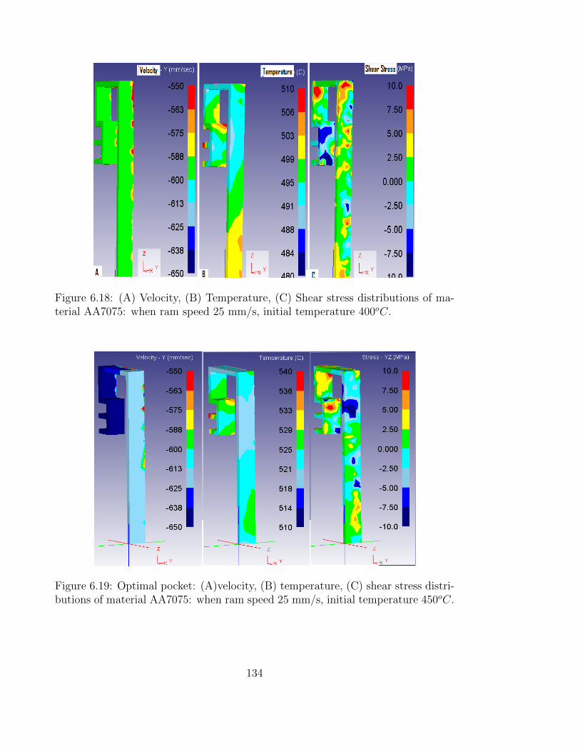
Figure 6.18: (A) Velocity, (B) Temperature, (C) Shear stress distributions of ma-terial AA7075: when ram speed 25 mm/s, initial temperature 400oC.
Figure 6.19: Optimal pocket: (A)velocity, (B) temperature, (C) shear stress distri-butions of material AA7075: when ram speed 25 mm/s, initial temperature 450oC.
134
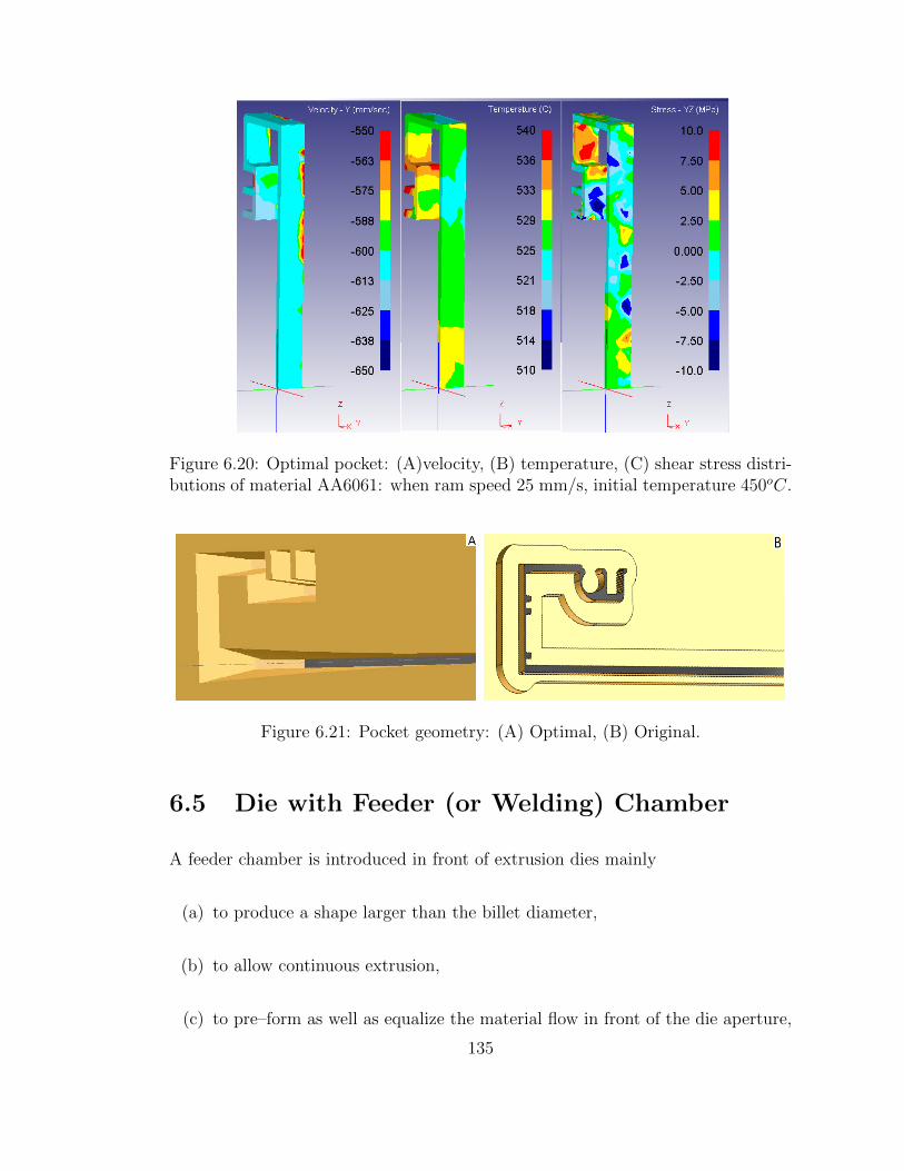
Figure 6.20: Optimal pocket: (A)velocity, (B) temperature, (C) shear stress distri-butions of material AA6061: when ram speed 25 mm/s, initial temperature 450oC.
Figure 6.21: Pocket geometry: (A) Optimal, (B) Original.
6.5 Die with Feeder (or Welding) Chamber
A feeder chamber is introduced in front of extrusion dies mainly
(a) to produce a shape larger than the billet diameter,
(b) to allow continuous extrusion,
(c) to pre–form as well as equalize the material flow in front of the die aperture,
135

and
(d) to spread the material flow [4].
Figure 6.22: Die with feeder chamber
The geometry of the die with feeder chamber considered for the investigation is
shown in Figure 6.22. The cross section of the feeder chamber is not very thin
and therefore the velocity across the surface is approximately constant everywhere.
Just before entering the die opening the aluminium inside the feeder chamber looks
like a slab of feeder chamber shape.
Figures 6.23 shows the velocity, temperature and shear stress distribution of the
extruded product between the entrance and exit of a die for the geometrical set unit
shown in Figure 6.22. It can be seen that the shear stress is very high at certain
positions and the velocity is not homogeneous. Figure 6.24 shows the homogeneity
of flow at three different locations(1, 2 and 3 as in Figure 6.22) along the longer
channel length. In this figure the flow patterns at the forming zone are not all
136

Figure 6.23: (A) Velocity, (B) Temperature, and (C) Shear stress inside the dieland
Figure 6.24: Velocity distribution at two different locations along the die channel,cut plane XY: (A) location 1, (B) location 2 , (C) location 3 of Figure 6.22
homogeneous and indicate that the ratio of w1 : w2 is not optimal to produce a
homogeneous flow. Further it has been found that the location of the higher shear
stress area is not the same for other simulation runs with different initial billet
137

Figure 6.25: Velocity distribution along the die channel without pocket
temperatures and ram speeds. Figure 6.25 shows the velocity distribution inside
the die land region for the die without pocket. Here it can be seen that even if the
channel length is significantly long, it did not result in such a big difference of flow
speeds along the channel length as in Figure 6.16 for the same die without feeder
chamber.
In the previous sections it has been already demonstrated that the homogeneity
of flow with a slant pocket die is much better than a rectangular pocket die and
therefore an investigation was conducted with a slant pocket and a procedure was
developed to determine the best possible geometry of a pocket to regulate the flow
through a die.
138

Figure 6.26: Sample die 2
6.5.1 Algorithm -3
The procedure consists of two steps. In the first step, the channel was divided
into 7 elements as shown in Figure 6.26. Since the velocity variation along the
longer channel is not very large compared to algorithm 1 and algorithm 2, only 4
elements along the longer channel were considered to save computation time. For
each element the optimal ratio w1 : w2 for well balanced flow is calculated by
running at least three simulations for various different w1 values for a fixed w2
value (or for various different w2 values for fixed w1 value). One such example
is shown in Figure 6.27. In this figure A, B, C and D respectively show the flow
velocity at either sides of elements 1, 2, 3 and 4.
In the second step, actual optimal values of w1 and w2 are calculated. It is done
by maintaining the same ratio obtained at step 1 for each element and running
simulations for various different w1 and w2 values until the velocity of flow across
each of seven elements are approximately the same. The algorithm consists of the
following steps:
1. Initialisation
(a) choose pocket depth d, bearing length b and one width w1;
139

Figure 6.27: Step 1 of Algorithm 3
(b) number of elements to be considered N .
(c) Initialize an array w2 of different w2 values with length of at least 3.
2. Calculate optimal ratio r = w1 : w2 for each element for which the velocity
across either side of the elements is equal.
(a) for i = 1 . . . 3
- w2 = w2(i)
- Run simulation and store velocity across either side of each element.
(b) Use linear regression to estimate the slope m[1 : N ] of flow velocity vs
w2 for each element.
140

(c) Estimate w2 for each element such that the velocity V[1 : N ] across
either side of element is equal.
3. (a) V ave =
∑V[1 : N ]
N; w1 = rw2
(b) for i = 1 : N
- if V[i]− V ave > tol
- w2[i] = w2[i]− δ
- else if V[i]− V ave < tol
- w2[i] = w2[i] + δ
4. Go to step 3 if ‖V − V ave‖ > 0 else Stop.
Figure 6.28 depicts the comparison of the shear stress distribution of the ex-
truded product of material AA7075 between the entrance and exit of an optimal
die and the original die. It can be seen that the shear stress distribution just out-
side the forming zone has been reduced dramatically. The optimal die is shown in
Figure 6.29.
6.6 Summary and Discussion
The goal of the work presented here is to identify the design and process parameters
which are more important for surface quality and to develop a suitable technique to
modify a die to minimize surface defects. It is an inverse problem and solved by a
finite element model and linear regression. In the process, three different algorithms
were developed, and applied to test cases.
A series of examples describes how the homogeneity of flow depends on the
geometry of the die pocket, and how the process parameters such as initial tem-
perature and ram speed influence the homogeneity of flow through a die which is
optimal for certain values of process parameters. The results from these examples
141

Figure 6.28: Shear stress distribution: (A) optimal die, (B) original die
Figure 6.29: Optimal die 2
142

suggest that the presented algorithms are capable of minimizing the velocity, tem-
perature and shear stress variation along the channel. Four factors which can be
used to alter the homogeneity of the flow are:
(i) initial temperature of billet,
(ii) channel length,
(iii) distance between die axis and channel axis, and
(iv) shape of the pocket.
From observations it can be noticed that the major factor that influences the flow is
the pocket geometry. Therefore it can be concluded that the surface quality of the
product can be optimised by designing a pocket suitable for the respective process
conditions.
143

144

Chapter 7
Comparison with Experimental
data
7.1 Experimental Trial
Experimental trials at an industrial plant were organised and conducted. This
chapter describes the equipment, trial procedure and sample preparation as well
as evaluation. For verification purposes a die optimized according to the design
algorithms mentioned in previous chapters has subsequently been manufactured
and run in a production extrusion press. The aim was to establish whether the
optimised die design delivers a high quality product free of flow lines on the flat
surface.
A billet being loaded in the extrusion press is shown in Figure 7.1. The billet is
a cylindrical shape of cast metal which is pushed through a die to extrude desired
shapes of uniform cross section. In this experimental investigation AA6061 alloy
which has a magnesium concentration of 0.40% was used. Before extrusion the billet
was preheated to 470oC by loading it into a preheating furnace for 40 minutes.
Figure 7-2 shows the extrusion profile extruding from the die exit. After extrud-
145

Figure 7.1: Cylindrical billet at the extrusion press.
Figure 7.2: Extrusion at the plant.
ing the part is clamped at either end lengthwise and a horizontal force is applied
to straighten it.
146

7.2 Investigation of Product Surface
Figure 7.3, and 7. 4 respectively show the photograph of the actual newly produced
part and the original old part. It can be seen with the naked eye that the usual die
lines appear and some slight streaks are also visible in the direction of the material
flow in the old and new part, although they are far less pronounced with the new
design. Streaks are differentiated by differences in the glossy appearance from their
surrounding surfaces. The surface gloss of materials is judged to be the amount
of incident light that is reflected at the specular reflectance angle of that surface.
The specular gloss is proportional to the reflectance of the surface. Materials with
smooth surfaces appear glossy and rough surfaces appear matte. All these are
dependent on the microstructure of the surface and any extent of flow-lines can
only be confirmed through micrographs.
Figure 7.3: Photograph of the newly produced part
Figure 7.4: Photograph of the original part.
147

Figure 7.5: Photograph of the newly produced part (which was etched for 20 min).
Figure 7.6: Photograph of the original part (which was etched for 17.5 min).
The next step of the examination is to find whether any grain size differences
exist in and out of the streak region. To examine that the surfaces of the extruded
samples had been etched for 5–20 minutes in a 10 % sodium hydroxide solution
and then their microstructure was analyzed with a scanning electron microscope
(SEM). Figure 7.5 and 7.6 respectively show the surfaces of samples given in figure
7.3 and 7.4 after etching with a sodium hydroxide solution. Samples considered of
each piece are labelled from 1 to 6 as shown in the figures 7.7-7.11 at 300X and
1000X magnification. In Figure 7.7, the areas 3 and 4 were judged as being the
most streaky ones, while areas 1 and 2 on the left hand side as well as areas 5 and
6 on the right hand side were seen as streak free surfaces.
The SEM pictures underneath reveal that the surface topography varied in
and out of the streak region in terms of surface matteness. The difference in mi-
148

Figure 7.7: New product: SEM images taken from six fields of view on the surfaceat 300X magnification. (5 minute etching in 10% Sodium Hydroxide).
149

Figure 7.8: New product: SEM images taken from six fields of view on the surfaceat 1000X magnification. (5 minute etching in 10% Sodium Hydroxide).
150

Figure 7.9: New product: SEM images taken from six fields of view on the surfaceat 300X magnification. (20 minutes etching in 10% Sodium Hydroxide).
151
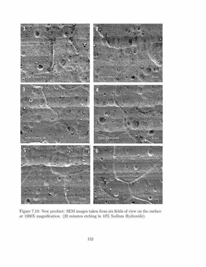
Figure 7.10: New product: SEM images taken from six fields of view on the surfaceat 1000X magnification. (20 minutes etching in 10% Sodium Hydroxide).
152

Figure 7.11: Original product: SEM images taken from six fields of view on thesurface at 300X magnification.
153

Figure 7.12: Original product: SEM images taken from six fields of view on thesurface at 1000X magnification.
154

crostructure within areas of the new piece are relatively small compared to within
the original piece. Therefore the optimised design has achieved its goal of providing
a more even material flow, which leads to a more homogeneous microstructure.
7.3 Image processing tool box - Matlab
Image processing generally involves extraction of useful information from an image.
The techniques used here are based on available literature [23]. Matlab’s image
processing tool box was used to investigate the SEM images from the previous
section. Initially Matlab’s in-built function, ‘im2bw’ was used to convert the images
to binary images; however the resulting images failed to distinguish between the
boundary and grain particles. The three colour channels (RGB) were found to give
better judgement to identify boundaries and grains. For each channel, intensity
thresholds were set above or below which pixels were defined as boundary or grains.
Boundary pixels were set to black and grain pixels to white to obtain a binary image.
Image restoration resulted in the boundaries between particles in very close
contact being lost. To repair this, holes in the images are filled by adjusting the
intensity levels of the surrounding pixels using morphological reconstruction. Once
the repair work is completed an in-built Matlab image segmentation algorithm
was used to detect particle edges and re-establish particle boundaries. The image
segmentation algorithm is a process of sorting a digital image into a number of
parts based on pixels properties. Each of the pixels in a region is similar with
respect to some characteristics, such as intensity, gradient and texture. Closest
regions are considerably different with respect to the same feature. The goal here
is to simplify the illustration of an image into objects that are more accurate and
easier to investigate.
The final binary image used for this investigation is shown in Figure 7.13. Par-
155

Figure 7.13: Binary image of Figure 7.7-3 after image reconstruction.
Figure 7.14: Final processed image of (A) Figure 7.7-3 and (B) Figure 7.11-3 usedfor investigation.
ticle centroids are marked with a cross and the particle index number in Figure
7.14. Once the grain particle cross section images were separated, the area of each
grain particle was calculated. The total number of particles identified and used in
the investigation of Figures 7.7-1, 7.7-2, 7.7-3, 7.11-1, 7.11-2 and 7.11-3 are given in
Figure 7.15A, 7.15B, 7.15C,7.15D, 7.15E and 7.15F respectively. It can be seen that
the difference in grain size area of the workpiece from the modified die is relatively
156

Figure 7.15: Particle counts from processed images of:(A) Figure 7.7-1, (B) Figure7.7-2, (C) Figure 7.7-3, (D) Figure 7.11-1, (E) Figure 7.11-2 and (F) Figure 7.11-3.
157

uniform compared to pictures of the workpiece manufactured with the old die.
7.4 Validation of FEA calculation
The following checks were done to confirm the accuracy and reliability of finite
element simulation work.
1. Initially similar problems given in the software manuals (Abaqus and Deform
3D) were compared with the simulation results in the manuals.
2. A very simple geometry model was solved using both software (Abaqus and
Deform 3D) and the simulation results were compared against each other.
3. The same model given in the literature [6], [18], [50] was modelled and the
simulation results were compared.
4. Implicit and explicit schemes were used and in different attempts yielding the
same results.
5. Inclusion of adaptive meshing improved the simulation speed maintaing ac-
curacy.
6. Element type and mesh density evaluated: Increased number of elements to
approach convergence. Same results obtained with different element types.
7. Model is solved using two different contact algorithms and yielding similar
results.
7.5 Summary and Discussion
The goal of this chapter is to examine whether the optimised die design delivers a
high quality product free of flow lines on the flat surface. To do that, the optimal
158

die shape which showed very even flow characteristics during the simulation has
been manufactured and run in a production extrusion press. The surface of the
extruded part shows the improved surface properties and a subsequent scanning
electron microscope analysis revealed very little variation in microstructure between
different surface regions of the final product.
159

160
Chapter 8
Summary and Conclusions
8.1 Summary
This thesis presents the development of procedures that can be used to find an
optimal set of conditions for an isothermal process to extrude a product for a
given shape and material properties with minimal defects. The solution process is
classified into the following:
1. Simple die geometry,
(a) Optimization of process and design parameters for given product quali-
ties.
(b) Estimation of grain size and material constants.
2. Complex die geometry.
Optimization of process and design parameters
(a) without feeder chamber
(b) with feeder chamber.
161

The developments of solution procedures for these cases are presented in chapters
4, 5 and 6. The developed procedures use the product geometry and material
data such as flow curve and microstructure during dynamic recrystallization as its
inputs.
Firstly, a small scale extrusion model was simulated using ABAQUS to study
the extrusion process in general. The following items were investigated.
1. How temperature, stress, strains and velocity changes during the extrusion
and how these quantities are related to die angle, die land length, friction,
material properties, initial billet temperature and extrusion speed.
2. How different solution schemes, adaptive meshing, different element type and
different contact algorithms influence the efficiency of the simulation.
Secondly a numerical technique to estimate the optimal die profile and the pro-
cess parameters for a simple geometry die was investigated. It is based on a non-
linear least squares coupled with finite element techniques. Nonlinear least squares
optimization is done by constructing an iterative procedure using MATLAB ’s inbuilt
function lsqnonlin and at each iteration, finite element solutions to the extrusion
flow are obtained using the ABAQUS FEA program.
Thirdly an inverse model to concurrently estimate the average grain size, ac-
tivation energy and other material constants appearing in the above optimization
function was developed. This method is not dependent on experimental observation
and it only uses simulated temperature and strain value history inside the defor-
mation zone. The method of the approach is based on a non-linear least squares
and Tikhonov’s regularisation method.
Fourthly, a complex geometry problem was considered. The finite element pro-
gram DEFORM 3D, which efficiently uses adaptive meshing controls to accommo-
date high workpiece deformations, is used to identify design and process parameters.
162

Three methods have been developed:
Method 1 Method 2 Method 3
(i) Obtained the flow (i) Obtained a linear (i) Obtained a ratio
velocity across relationship between between the pocket
each element (1:n) widths and speeds widths for each
for the die for each element. element which gives
with no pocket. well balanced flow
across the die
opening.
(ii) Obtained the (ii) Obtained widths (ii) By maintaining the
widths of the of each element ratio obtained from
elements 2 to n which gives the step 1 calculated the
which gives the same speed optimal values of
same flow as across the die pocket widths for
element 1 opening. each element to
achieve a uniform
speed across the
(iii) Pocket shape is (iii) Obtained the outer opening.
obtained for the shape of the pocket
well balanced which gives well
uniform flow across balanced uniform
the die opening. speed across the.
die opening.
All three methods perform well; one particular approach does not always predict
a better result than the other method. Therefore all three methods are equally
useful. If only the amount of computation time is considered, then method 3 is a
163

better choice than the other two methods.
Finally experimental trials at an industrial plant were conducted. These experi-
ments were done to verify the theoretical prediction described in previous chapters.
8.2 Conclusions
The main objective of the work presented here is to identify the design and process
parameters which are most important for surface quality to extrude a complex
geometry product with 6XXX and 7XXX series aluminium alloys. In the process
suitable computational techniques were developed to modify an existing die to
minimize surface defects. Then the newly designed die has been manufactured and
run in a production extrusion press. The main contributions towards resolving this
problem are:
1. The surface of the extruded part shows more homogeneous surface properties
and a subsequent scanning electron microscope analysis revealed very little
variation in microstructure between different surface regions of the newly
developed product.
2. The newly developed die is capable of extruding a product with relatively
small variation of velocity, temperature and shear stress across the channel.
3. Four factors which can be used to alter the homogeneity of the flow are (i)
initial temperature of billet, (ii) channel length, (iii) distance between die axis
and channel axis, and (iv) shape of the pocket. It can be noticed from obser-
vations that the major factor that influences the flow is the pocket geometry.
Therefore it can be concluded that the surface quality of the product can be
optimised by designing a pocket suitable for the respective process conditions.
164

4. The efficiency of the simulation results hugely depends on (a) solution meth-
ods (b) iteration method and (c) step controls since the problems considered
here have a complex geometry and thin profiles, which necessitate large billet
area reductions and sharp corners which require frequent remeshing during
the simulation of the extrusion process.
5. It has been demonstrated that finite element analysis is an efficient tool to
predict the deformation behaviour and the following has been established:
(a) The tendency toward chevron cracking is not observed (hydrostatic pres-
sure inside the forming zone is not zero) with a die shape that minimizes
one or more of the following: extrusion pressure, temperature variation,
and strain rate variation.
(b) The possibility of surface cracking can be avoided by designing a die,
which minimizes the strain rate variation, velocity variation at the exit
and the extrusion pressure.
(c) The optimal parameter values are not the same (eg the parameters which
minimizes the extrusion pressure are not same as the parameters which
minimizes temperature variation inside the die) for all categories.
(d) The grain size is more sensitive to extrusion speed and the initial tem-
perature than die geometry.
(e) The uniformity of the grain structure is more influenced by the shape of
the die surface than the initial temperature or ram speed.
(f) Surface quality of the simple geometry product can be optimised by
altering the flow through the die using Bezier curves with five control
points and optimising process conditions.
165

8.3 Future Experimental work
The main purpose of this thesis was a theoretical study of the process of aluminium
extrusion and the results have been verified towards the end of the project in a
factory trial of an improved version of a production die. The original production
die had created surface imperfections in terms of flow lines and was a difficult profile
to extrude because of a high extrusion ratio. Since the verification took place in
a factory environment, the opportunities for gathering ample process data were
limited.
To further confirm the accuracy of the simulation work it would be desirable
to conduct a similar extrusion process in a laboratory environment and record and
compare a number of process input and output parameters.
1. The speed and force of the extrusion press should be continuously recorded.
The billet temperature profile should be measured as well as the exit temper-
ature of the extruded material behind the die.
2. The process conditions of press speed and billet temperature should be varied
within feasible limits to be able to assess, whether the simulation model shows
the same sensitivity as the real process.
3. After each trial run the grain sizes should be determined on the surface of
the product as well as internally and the uniformity or lack of it should be
assessed.
166

8.4 Future Research
This research establishes a foundation for future work. In particular, the following
items are still requiring clarification:
(i) In Chapter 6 it has been learned that the homogeneity of flow with a curved
pocket die is much better than a slant or rectangular pocket die. The curved
pocket can be constructed using a series of Bezier curves along the channel
sides as in Figure 8.1 and therefore it is possible to extend the method devel-
oped for a simple geometry die. This can be incorporated into our algorithm
easily, but considering more Bezier curves along the channel will increase the
number of design parameters considerably and it is computationally currently
very expensive and it is not possible to complete the task within a resonable
time frame. This is one area where the model could be improved.
(ii) A model developed for one specific geometry cannot be directly applied for
another geometry. If a parameterised model can be developed suitable for
a wide range of geometries then by changing necessary parameter values it
will be possible to predict an optimal set of values of process and design
parameters. This would be of further benefit for industrial applications.
Figure 8.1: Bezier curved die
167

168

Appendix A
Appendix: Programming Codes
Python programming codes
from abaqus import *
from abaqusConstants import *
session.Viewport(name=’Viewport: 1’, origin=(0.0, 0.0), width=225.0,
height=186.46875)
session.viewports[’Viewport: 1’].makeCurrent()
session.viewports[’Viewport: 1’].maximize()
from driverUtils import executeOnCaeStartup
executeOnCaeStartup()
import visualization
import xyPlot
import displayGroupOdbToolset as dgo
o2 = session.openOdb(name=’Abaqus-file-name.odb’)
session.viewports[’Viewport: 1’].setValues(displayedObject=o2)
169

odb = session.odbs[’Abaqus-file-name.odb’]
session.xyDataListFromField(odb=odb, outputPosition=NODAL, variable=
((’S’, INTEGRATION_POINT, ((INVARIANT, ’Pressure’), )), ),
nodeSets=(’PART-1-1.TOP’, ),steps=(’Step-1’,’Step-2’))
###
xy1 = session.xyDataObjects[’S:Pressure PI: PART-1-1 N: 831’]
xy2 = xy1*1
session.XYData(name=’S’, objectToCopy=xy2,
sourceDescription=’"S:Pressure PI: PART-1-1 N: 831" * 1’)
xy1 = session.xyDataObjects[’S’]
session.writeXYReport(fileName=’TOPpressure.xls’, appendMode=OFF,
xyData=(xy1, ))
####
session.xyDataListFromField(odb=odb, outputPosition=NODAL, variable=
((’NT11’, NODAL,), ), nodeSets=(’PART-1-1.ALL’,
),steps=(’Step-1’,’Step-2’))
xy1 = session.xyDataObjects[’NT11: PI: PART-1-1 N: 574’]
xy2 = xy1*1
session.XYData(name=’NT11’, objectToCopy=xy2,
sourceDescription=’"NT11: PI: PART-1-1 N: 574" * 1’)
xy1 = session.xyDataObjects[’NT11’]
session.writeXYReport(fileName=’Tem574.xls’, appendMode=OFF,
xyData=(xy1, ))
####
session.xyDataListFromField(odb=odb, outputPosition=NODAL, variable=
170

((’PEEQ’, INTEGRATION_POINT, ), ), nodeSets=(’PART-1-1.ALL’,
),steps=(’Step-1’,’Step-2’))
xy1 = session.xyDataObjects[’PEEQ: PI: PART-1-1 N: 574’]
xy2 = xy1*1
session.XYData(name=’PEEQ’, objectToCopy=xy2,
sourceDescription=’"PEEQ: PI: PART-1-1 N: 574" * 1’)
xy1 = session.xyDataObjects[’PEEQ’]
session.writeXYReport(fileName=’peeq574.xls’, appendMode=OFF,
xyData=(xy1, ))
####
session.xyDataListFromField(odb=odb, outputPosition=NODAL, variable=
((’S’, INTEGRATION_POINT, ((COMPONENT, ’S22’), )), ),
nodeSets=(’PART-1-1.ALL’, ),steps=(’Step-1’,’Step-2’))
xy1 = session.xyDataObjects[’S:S22 PI: PART-1-1 N: 538’]
xy2 = xy1*1
session.XYData(name=’S’, objectToCopy=xy2,
sourceDescription=’"S:S22 PI: PART-1-1 N: 538" * 1’)
xy1 = session.xyDataObjects[’S’]
session.writeXYReport(fileName=’s22-538.xls’, appendMode=OFF,
xyData=(xy1, ))
session.xyDataListFromField(odb=odb, outputPosition=NODAL, variable=
((’CPRESS’, ELEMENT_NODAL,), ), nodeSets=(’PART-1-1.CONTACT’,
),steps=(’Step-1’,’Step-2’))
####
xy1 = session.xyDataObjects[’CPRESS: PI: PART-1-1 N: 1’]
xy2 = xy1*1
session.XYData(name=’CPRESS’, objectToCopy=xy2,
171

sourceDescription=’"CPRESS: PI: PART-1-1 N: 1" * 1’)
xy1 = session.xyDataObjects[’CPRESS’]
session.writeXYReport(fileName=’CPRESS01.xls’, appendMode=OFF,
xyData=(xy1, ))
####
session.xyDataListFromField(odb=odb, outputPosition=NODAL, variable=
((’U’, NODAL, ((COMPONENT, ’U2’), )), ),
nodeSets=(’PART-1-1.ALL’, ),steps=(’Step-1’,’Step-2’))
xy1 = session.xyDataObjects[’U:U2 PI: PART-1-1 N: 496’]
xy2 = xy1*1
session.XYData(name=’U’, objectToCopy=xy2,
sourceDescription=’"U:U2 PI: PART-1-1 N: 496" * 1’)
xy1 = session.xyDataObjects[’U’]
session.writeXYReport(fileName=’U2496.xls’, appendMode=OFF,
xyData=(xy1, ))
###
session.xyDataListFromField(odb=odb, outputPosition=NODAL, variable=
((’V’, NODAL, ((COMPONENT, ’V2’), )), ),
nodeSets=(’PART-1-1.ALL’, ),steps=(’Step-1’,’Step-2’))
xy1 = session.xyDataObjects[’V:V2 PI: PART-1-1 N: 496’]
xy2 = xy1*1
session.XYData(name=’V’, objectToCopy=xy2,
sourceDescription=’"V:V2 PI: PART-1-1 N: 496" * 1’)
xy1 = session.xyDataObjects[’V’]
session.writeXYReport(fileName=’V2496.xls’, appendMode=OFF,
xyData=(xy1, ))
####################
172
Matlab programming codes
function [x,y]=Beziergraph(n,X,Y)
%n=number of points required
%(X,Y) are 5 Control points of Beziercurve
N=length(X);
t=0:1/(n-1):1;
x=zeros(1,n);y=zeros(1,n);
for i=1:n
b=bernstein_basis(N-1,t(i));
x(i)=sum(X.*b);y(i)=sum(Y.*b);
end
R0=0.10;Rf=0.0666;m1=2;
P1X=R0;P2X=R0;P4X=Rf;P5X=Rf;
P1Y=-0.01;
P2Y=-0.07;
P3Y=-0.07;
P4Y=-0.16;
P5Y=-0.16;
n2=length(P2Y);n4=length(P4Y);
n5=length(P5Y);n3=length(P3Y);
MY=zeros(n2*n3*n4*n5,5);MX=zeros(n2*n3*n4*n5,5);
MY(:,1)=P1Y;MX(:,1)=P1X;
nn=n2*n3*n4*n5;
s=1;
for i=1:n2
173

for j=1:n3
for k=1:n4
for l=1:n5
MY(s,5)=P5Y(l);MX(s,5)=P5X;
MY(s,4)=P4Y(k);MX(s,4)=P4X;
MY(s,3)=P3Y(j);
MY(s,2)=P2Y(i);MX(s,2)=P2X;
MX(s,3)=Rf+(R0-Rf)*(MY(s,4)-MY(s,3))/(MY(s,4)-MY(s,2));
s=s+1;
end
end
end
end
n=23;
z=1:1:165;
EP=zeros(1,nn);
PEEQ=zeros(4,nn);
TEM=zeros(1,nn);
S11=zeros(1,nn);
S22=zeros(1,nn);
DP1=zeros(21,nn);
DP2=zeros(21,nn);
U2=zeros(11,nn);
V2=zeros(11,nn);
PEEQ1=zeros(11,nn);
PEEQ1dot=zeros(11,nn);
for i=1:nn
174

[x,y]=Beziergraph(n,MX(i,:),MY(i,:));
%~~~~~~~~~~~~~~~~~~~~~~~~~~~~~~~~~~~~~~~~~~~~~~~~~~~~~~~~~~~~~~~~~~~~~~~~~~
fid = fopen(’dienode1.inp’,’w’);
fprintf(fid,’%4d, %3.4f, %3.4f\n’, z(1), x(1), y(1));
fprintf(fid,’%4d, %3.4f, %3.4f\n’, z(59), x(2), y(2));
fprintf(fid,’%4d, %3.4f, %3.4f\n’, z(60), x(3), y(3));
--
--
--
fclose(fid);
%~~~~~~~~~~~~~~~~~~~~~~~~~~~~~~~~~~~~~~~~~~~~~~~~‘
!abaqus job=file-Name interactive
!abaqus cae nogui=filename.py
ncols=2;nhead=2;nlrows=10;
fin = fopen(’Excel-file-name.xls’,’r’);
for j=1:nhead, buffer = fgetl(fin); end
data = fscanf(fin,’%f’);
nd = length(data); % total number of data points
nr = nd/ncols;
data = reshape(data,ncols,nr)’; % notice the transpose operator
y = data(:,2:ncols);
nl=length(y);
175

EP(1,i)=sum(y)/nl;
176

Bibliography
[1] Arentoft M., Gronostajski Z., Niechajowicz. A., and Wanheim T., Physical and
mathematical modelling of extrusion process, Journal of Materials Processing
Technology, 106, 2–7, 2000.
[2] Antunez H. J., Thermo-mechanical modelling and sensitivity analysis for
metal-forming operations, Computer Methods in Applied Mechanics and En-
gineering 161(1-2): 113–125, 1998.
[3] Balendra R., Qin Y., and Chodnikiewicz K., Analysis of temperature and
from-error variation with the manufacturing cycle during the forward extrusion
components, Journal of Materials Processing Technology, 145, 171–179, 2004.
[4] Bauser M., Sauer G., and Siegert K., Extrusion, ASM publications, 2006.
[5] Bhattacharyya D., Richards P. J., Modelling of metal extrusion using the
phonix package, Journal of Materials Processing Technology, 35(1), 93–111,
1992.
[6] Chanda T., Zhou J., and Duszczyk. J., A comparative study on iso-speed
extrusion and isothermal extrusion of 6061 Al alloy using 3D FEM simulation,
Journal of Materials Processing Technology, 114, 145–153, 2001.
[7] Chanda T., Zhou J., and Duszczyk. J., Application of three-dimensional nu-
merical simulation to analysis of development of deformation zone at beginning
177

of aluminium extrusion process, Materials science and Technology, 17, 70–74,
2001.
[8] Chanda T., Zhou J., and Duszczyk. J., FEM analysis of aluminium extrusion
through square and round dies, Materials and Design, 21, 323–335, 2000.
[9] Chang C. I., Lee C. J., and Huang J. C., Relationship between grain size and
ZenerHolloman parameter during friction stir processing in AZ31 Mg alloys,
Scripta Materialia, 51, 509–514, 2004.
[10] Cho J. R., Bae W. B., Hwang W. J., and Hartley P., A study on the hot
deformation behaviour and dynamic recrystallization of Al-5 wt %Mg alloy,
Journal of material processing technology, 118, 356–361, 2001.
[11] De Pari Jr. L, Misiolek W. Z., Theoretical predictions and experimental verifi-
cation of surface grain structure evolution for AA6061 during hot rolling, Acta
Materialia 56, 6174-6185, 2008.
[12] Dieter G. E., Semiatin S. L., and Kuhn H, Handbook of Workability and
Process Design, ASM International, 2002.
[13] Duan X., and Sheppard T., Simulation and control of microstructure evolu-
tion during hot extrusion of hard aluminium alloys, Materials Science and
Engineering, 351, 282–292, 2003.
[14] Duan X., and Sheppard T., Modelling and Simulation in Material Science and
Engineering, 10(4), 363–380, 2002.
[15] Fang G., Zhou J., Duszczyk J., and Wu. X. K, FE simulation of extrusion
to produce a thin-walled wide profile through a spreading pocket die, Key
Engineering Materials, 367, 63–70, 2008.
178

[16] Fang G., Zhou J.,, Duszczyk J., Extrusion of 7075 aluminium alloy through
double-pocket dies to manufacture a complex profile, Journal of Materials
Processing Technology, 209, 3050–3059, 2009.
[17] Fernandes J. L. M., Rodrigues J. M. C., and Martins P. A. F., Combined
finite elementboundary element thermo-mechanical analysis of metal forming
processes Journal of Materials Processing Technology, 87, 247-257, 1999.
[18] Flitta I and Sheppard T., Nature of friction in extrusion process and its effect
on material flow, Materials Science and Technology, 19, 837–846, 2003.
[19] Gardner J. D., and Dornfeld D., Finite Element Modeling of Drilling Using
DEFORM, Laboratory for Manufacturing and Sustainability, Consortium on
Deburring and Edge Finishing, June, 2006.
[20] Gejadze I., and Jarny Y., An inverse heat transfer problem for restoring the
temperature field in a polymer melt flow through a narrow channel, Interna-
tional Journal of Thermal Sciences, 41, 528-535, 2002.
[21] Gierzynska-Dolna M., and Lacki P., Some aspects of modelling of metal form-
ing processes, Computers & Structures, 81, 605–613, 2003.
[22] Golovko O., Grydin O., Method for pocket die design on the basis of numerical
investigations of aluminium extrusion process, Metalurgija, 45(3), 155–161,
2006.
[23] Gonzalez R., Wood R., and Eddins S., Digital image processing using MAT-
LAB, 2004.
[24] Gouveia B. P. P. A., Rodrigues J. M. C., Bay. N., and Martins P. A. T., Finite-
element modelling of cold forward extrusion, Journal of Materials Processing
Technology, 94, 85–93, 1999.
179

[25] Gouveia B. P. P. A., and Rodrigues J. M. C, Physical modelling and numeri-
cal simulation of the round-to-square forward extrusion, Journal of Materials
Processing Technology, 112, 244–251, 2001.
[26] Gouveia B. P. P. A., and Rodrigues J. M. C., Finite-element modelling of
cold forward extrusion, Journal of Materials Processing Technology, 94, 85–
93, 1999.
[27] Gouveia B. P. P. A., and Rodrigues J. M. C., Steady-state finite-element anal-
ysis of cold forward extrusion, Journal of Materials Processing Technology, 73,
281–288, 1998.
[28] Gouveia B. P. P. A., and Rodrigues J. M. C., Finite element modelling of
cold forward extrusion using updated Lagrangian and combined Eulerian-
Lagrangian formulations, Journal of Materials Processing Technology, 80-81,
647-652, 1998.
[29] Hansen C. P., Rank-deficient and discrete ill-posed problems, SIAM, Philadel-
phia, PA, 1997.
[30] Hansen C. P., Regularization tools: A MATLAB package for analysis and so-
lution of discrete ill-posed problems, Danish Computing Center for Research
and Education, 1993.
[31] HE You-feng, XIE Shui-sheng, CHENG Lei, HUANG Guo-jie, FU Yao, FEM
simulation of aluminum extrusion process in porthole die with pockets, Trans
Nonferrous Met Soc China, 20, 1067–1071 2010.
[32] Kathirgamanathan P., and Neitzert T., Optimization Method of Extrusion
Dies, Submitted to Production Engineering Research & Development.
180

[33] Kathirgamanathan P., and Neitzert T., Optimization of pocket design to pro-
duce a thin shape complex profile, Production Engineering Research & Devel-
opment, 3-3, 231–241, 2009.
[34] Kathirgamanathan P., and Neitzert T., Inverse Modelling for Estimation of
Average Grain Size and Material Constants - An Optimization Approach, Lec-
ture Notes in Engineering and Computer Science, 2, 850–854, 2008.
[35] Kathirgamanathan P., and Neitzert T., Optimal process control parameters
estimation in aluminium extrusion for given product characteristics, Lecture
Notes in Engineering and Computer Science, 2, 1436–1441, 2008.
[36] Kathirgamanathan P., and Neitzert T., Modelling of metal extrusion using
ABAQUS, The Proceedings of 3rd NZ Metals Industry Conference 2006.
[37] Lee S. K., Ko D. C., and Kim B. M., Optimal die profile design for uniform
microstructure in hot extruded product, International Journal of Machine Tools
& Manufacture, 40, 1457–1478, 2000.
[38] Lee G., Kwak D. M, Kim S., Im I., Analysis and design of flat-die hot extrusion
process, International Journal of Mechanical Sciences, 44, 915-934, 2002.
[39] Li F., Yuan S. J., He Z. B., Research of metal flow behavior during extrusion
with active friction, JMEPEG, 17, 7-14, 2008.
[40] Li S., Bourke M. A. M., Finite element analysis of the plastic deformation zone
and working load in equal channel angular extrusion, Materials Science and
Engineering, 382(1-2), 217-236, 2004.
[41] Li H. J., Qi L. H., Neural network modeling and optimization of semi-solid
extrusion for aluminum matrix composites, Journal of Materials Processing
Technology, 151(1-3), 126–132, 2004.
181
[42] Li L., Zhou J., Prediction of temperature evolution during the extrusion of
7075 aluminium alloy at various ram speeds by means of 3D FEM simulation,
Journal of Materials Processing Technology, 145(3), 360–370, 2004.
[43] Li L., Zhou J., and Duszczyk J., A 3D FEM simulation study on the isother-
mal extrusion of a 7075 aluminium billet with a predetermined non-linear
temperature distribution, Modelling and Simulation in Materials Science and
Engineering, 11, 401–416, 2003.
[44] Li Q., Smith C. J., Harris C., and Jolly M. R., Finite element investigations
upon the influence of pocket die designs on metal flow in aluminium extrusion
Part 1. Effect of pocket angle and volume on metal flow, Journal of Materials
Processing Technology, 135, 189–196, 2003.
[45] Li Q., Smith C. J., Harris C., and Jolly M. R., Finite element investigations
upon the influence of pocket die designs on metal flow in aluminium extrusion
Part 2. Effect of pocket geometry configurations on metal flow, Journal of
Materials Processing Technology, 135, 197–203, 2003.
[46] Li L., Zhou J., and Duszczyk J., A 3D FEM simulation study on the isother-
mal extrusion of a 7075 aluminium billet with a predetermined non-linear
temperature distribution, Modelling and Simulation in Materials Science and
Engineering, 11, 401-416, 2003
[47] Li L. X., and Rao K. P., A study on hot extrusion of Ti-6Al-4V using simula-
tions and experiments, International Journal of Mechanical Sciences, 44(12),
2415–2425, 2002.
[48] Lia L. X., Rao K. P., Lou Y., and Peng D. S., A study on hot extrusion of
Ti6Al4V using simulations and experiments, International Journal of Mechan-
ical Sciences, 44, 2415-2425, 2002.
182

[49] Lin Z., and Juchen X., Optimization of die profile for improving die life in
the hot extrusion process, Journal of Materials Processing Technology, 142(3),
659–664, 2003.
[50] Lof J., Developments in finite element simulations of aluminium extrusion,
PhD Thesis, University of Twente, The Netherlands, 2000.
[51] Lof J., and Blokhuis Y., FEM simulations of the extrusion of complex thin-
walled aluminium sections, Journal of Materials Processing Technology, 122,
344–354, 2002.
[52] Lu J., and Saluja N., Computer modeling of the continuous forming extrusion
process of AA6061 alloy, Journal of Materials Processing Technology, 79(1-3),
200–212, 1998.
[53] Malas J. C., Frazier W. G., Venugopal S., Medina A., Medeiros S., Srinivasan
R., Irwin D., Mullins W. M., and Chaudhary A., Optimization of microstruc-
ture development during hot working using control theory, Metallurgical and
Materials Transactions A, 28, 1921–1930, 1997.
[54] Mathews j. H., and Fink K. D., Numerical Methods Using Matlab, Prentice-
Hall Inc, 4-th Edition, 309–317, 2004.
[55] Muramatsu T., Zhang S., Lim B., and Yong S., Study on Flexi-Extrusion
Forging Technique by Using Intelligent Actuating Tooling, SIMTech Technical
Report, 2005.
[56] Nes E., Marthinsen K., Modelling the evolution in microstructure and prop-
erties during processing of aluminium alloys, Journal of Materials Processing
Technology, 117(3), 333–340, 2001.
183

[57] Peng Z., and Sheppard T., A study on material flow in isothermal extrusion
by FEM simulation, Modelling and Simulation in Materials Science and En-
gineering, 12, 745–763, 2004.
[58] Peris R., Effects of extrusion conditions on ”Die Pick-Up” formed during ex-
trusion of aluminium alloy AA6060, Masters Theses, 2007.
[59] Reddy V. R., Sethuraman R., Lal G. K., Upper-bound and finite-element
analysis of axisymmetric hot extrusion, Journal of Materials Processing Tech-
nology, 57, pp.14–22, 1996.
[60] Reddy J. N., Energy principles and variational methods in applied mechanics,
NWiley, New York, 2002.
[61] Rodrigues J. M. C., and Martins P. A. F., Coupled thermo-mechanical anal-
ysis of metal-forming processes through a combined finite elementboundary
element approach, International Journal for Numerical Methods in Engineer-
ing, 42, 631–645, 1998.
[62] Rodriguez, A., Rodriguez, P., System to calculate chambers and feeds to obtain
a minimum single bearing, Proceedings of the Fifth International Aluminium
Extrusion Technology, 1, 283–290, 1992.
[63] Rodriguez, A., Rodriguez, P., Process and system of calculation for construc-
tion of dies for extrusion of solid aluminium profiles, United States Patent
5870922, 1999.
[64] Saha P. K., Thermodynamics and tribology in aluminum extrusion, Wear,
218(2), 179–190, 1998.
[65] Saha P. K., Aluminum Extrusion Technology, ASM publications, 2000.
184

[66] Sheppard T., Prediction of structure during shaped extrusion and subsequent
static recrystallization during the solution soaking operation, Journal of ma-
terial processing technology, 177, 26–36, 2006.
[67] Shivpuri R., Advances in numerical modelling of manufacturing process,
TransIndian Inst Metals, 57(4), 345–366, 2004.
[68] Sliwa R., and Zasadzii H. J., Surface cracking of bars in the metal extrusion
process: part 1, Journal of Mechanical Working Technology, 14, 325–341.
[69] Sofuoglu H., and Gedikli H., Physical and numerical analysis of three dimen-
sional extrusion process, Computational Materials Science, 31(1-2), 113-124.
[70] Storen S., The theory of extrusion–Advances and challenges, International
Journal of Mechanical Sciences, 35(12), 1007-1020.
[71] Sun Y., Gupta M., Optimization of flat die geometry, ANTEC, 50, 3307–3311,
2004.
[72] Tiernan P., and Hillery M. T., Modelling of cold extrusion with experimen-
tal verification, Journal of Materials Processing Technology, 168(2), 360–366,
2005.
[73] Ulrich Aluminium, Hamilton, New Zealand, www.ulrich-aluminium.co.nz-
August 2008.
[74] Ulysse P., Optimal extrusion die design to achieve flow balance, International
Journal of Machine Tools and Manufacture, 39(7), 1047–1064, 1999.
[75] Valberg H., Applied Metal Forming: including FEM analysis, Cambridge Uni-
versity Press, 2010.
185
[76] Venugopal S., Medina E. A., Malas I., Medeiros S., and Frazier W. G., Opti-
mization of microstructure during deformation processing using control theory
principles, Scripta materialia, 36, 347–353, 1997.
[77] Venugopal S., and Rodriguez P., Strategy for the design of thermomechanical
processes for AISI type 304L stainless steel using dynamic materials model
stability criteria and model for the evolution of microstructure, Journal of
Materials Science, 39, 5557–5560, 2004.
[78] Wifi A. S., Shatla M. N., and Abdel-Hamid., An optimum-curved die profile
for the hot forward rod extrusion process, Journal of Materials Processing
Technology, 73, 97–107, 1998.
[79] Wang L., Yang H., Frictioninal miniumextrusion-part 2: A review of friction
models for aluminium extrusion, Tribology International 56, 99–106, 2012.
[80] Williams A. J., Computational modelling of metal extrusion and forging pro-
cess, Journal of Materials Processing Technology, 125-126, 573–582, 2002.
[81] Yuan Z., Li F., and He Z., Effects of guiding angle on plastic metal flow
and defects in extrusion of aluminium alloy, Journal of Materials Science and
Technology, 24, 256–260, 2005.
[82] Zheng P. F., and Chan L. C., Numerical analysis of the sheet metal extrusion
process, Finite Elements in Analysis and Design, 42(3), 189–207, 2005.
[83] Yan H., and Xia J., An approach to the optimal design of technological pa-
rameters in the profile extrusion process, Science and Technology of Advanced
Materials, 7, 127–131, 2006.
186

[84] Zhou J., and Li L., Computer simulated and experimentally verified isothermal
extrusion of 7075 aluminium through continuous ram speed variation, Journal
of Materials Processing Technology, 146(2), 203–212, 2004.
[85] Zhou J., and Li L., 3D FEM simulation of the whole cycle of aluminium extru-
sion throughout the transient state and the steady state using the updated La-
grangian approach, Journal of Materials Processing Technology, 134(3), 383–
397, 2003.
[86] Zhou L., Li. J., and Duszczyk J., A 3D FEM simulation study on the isother-
mal extrusion of a 7075 aluminium billet with a predetermined non-linear
temperature distribution, Modelling and Simulation in Materials Science and
Engineering, 11, 401–416, 2003.
187