Parameter-Free Fast Pixelwise Non-Local Means Denoising

Published in Image Processing On Line on 2014–11–19.Submitted on 2014–07–18, accepted on 2014–08–05.ISSN 2105–1232 c© 2014 IPOL & the authors CC–BY–NC–SAThis article is available online with supplementary materials,software, datasets and online demo athttp://dx.doi.org/10.5201/ipol.2014.120

2014/07/01

v0.5

IPOL

article

class

Parameter-Free Fast Pixelwise Non-Local Means Denoising

Jacques Froment

Univ. Bretagne - Sud, UMR 6205, LMBA, F-56000 Vannes, France ([email protected])

Abstract

This article proposes a fast and open-source implementation of the well-known Non-Local Means(NLM) denoising algorithm, in its original pixelwise formulation. The fast implementation isbased on the computation of patch distances using sums of lines that are invariant under apatch shift. The optimal parameters of NLM (in the average peak signal to noise ratio - PSNR- sense) are computed from an image database, thereby leading to a parameter-free NLM imple-mentation. Comparison is performed with the parameter-free blockwise NLM implementationalready proposed in IPOL journal by Buades, Coll and Morel. As expected the blockwise imple-mentation offers better PSNR, at least when the noise standard deviation is large enough, butthere is no significant difference in quality when performing visual inspection. The highlight isthat the proposed parameter-free pixelwise NLM implementation is faster than the patchwiseone by a factor of 6 to 49.

Source Code

The reviewed source code and documentation for the parameter-free fast pixelwise NLM algo-rithm are available from the web page of this article1. Compilation and usage instructions areincluded in the README.txt file of the archive.

Keywords: image denoising; non-local means

1 Introduction

The Non-Local Means (NLM) image denoising algorithm was introduced in 2005 by Antoni Buades,Bartomeu Coll and Jean-Michel Morel [1] and the success was such that this method has inspireda great number of variants and articles, see [3] for some updated references. Three factors largelyexplain why the image denoising community has been immersed in the NLM approach: the originalalgorithm remains simple; it provides great visual quality; it introduces a basic tool to exploitthe non-local redundancy of natural images. Despite the subsequent introduction of more efficientdenoising algorithms (see [20, 16] for recent comparisons between NLM and some state of the artdenoising schemes), NLM remains a reference method for image denoising. It is therefore essential

1http://dx.doi.org/10.5201/ipol.2014.120

Jacques Froment, Parameter-Free Fast Pixelwise Non-Local Means Denoising, Image Processing On Line, 4 (2014), pp. 300–326.http://dx.doi.org/10.5201/ipol.2014.120

http://dx.doi.org/10.5201/ipol

http://dx.doi.org/10.5201/ipol

http://creativecommons.org/licenses/by-nc-sa/3.0/

http://dx.doi.org/10.5201/ipol.2014.120




that the image denoising community has freely available a documented, verified and open-sourceimplementation of NLM in its original version.

Despite the number of NLM codes that can be found in the Internet, it seems that there are onlytwo implementations that fulfill these conditions: the nlmeans module included in MegaWave2 [11]and written by Lionel Moisan and the IPOL article [4] from Buades, Coll and Morel. The first codeimplements the pixelwise NLM algorithm given in [1] (Section 5.1) for gray-level images only andusing the Euclidean norm instead of the uniform one to define neighbor patches. The parameters’default values correspond to those in [1], but they turn out to be non optimal for most images.Finally, this code does not implement any algorithmic trick or parallelization of computing, makingit a slow running program. While the IPOL article [4] describes both the pixelwise NLM (NLM-P)([1] Section 5.1) and the blockwise NLM (NLM-B) ([1] Section 5.5.2), the published demo and codeimplement the blockwise version only2.

The present article aims to propose a fast and parameter-free implementation of the pixelwiseNLM as described in [1] (pages 510-512). In order to fix the notation, let us first recall the equationsthat lead to this algorithm.

The input, noisy image v, is assumed to come from the classical additive noise model

v(x) = u(x) + ǫ(x), x ∈ Ω, (1)

where u is the original image, Ω is the set of pixels and ǫ is the noise perturbation: (ǫ(x))x∈Ωare independent and identically distributed (i.i.d.) Gaussian variables with mean 0 and standarddeviation σ > 0. In the case of gray-level images, u and v take real values (integer values in thediscrete model) whereas for color images, u and v are vector-valued.

The output, denoised image, is the estimator u computed as

u(x) =∑

y∈Ωx

w(x, y)v(y), (2)

where the weight w(x, y) estimates the similarity between the pixel x and y in the original imageand the sequence of weights satisfies

w(x, y) ≥ 0 and∑

y∈Ωx

w(x, y) = 1, ∀x ∈ Ω, y ∈ Ωx. (3)

The set of pixels Ωx is a neighborhood of x ∈ Ω, it is defined as

Ωx = y ∈ Ω : ‖x− y‖∞ ≤ D, (4)

for D > 0 a fixed size parameter. The window Ωx is called the search window at x and, for simplicityand faster computations, in [1] a choice of a square shape of fixed size is made while, according toauthors, the search window should cover the entire image plane, hence the non-local nature of thealgorithm. However, it has been reported that using for NLM a neighborhood instead of the wholeimage plane allows to increase the denoising performance [12, 13, 21, 22], see also the discussion in [9]and the specific study in [19] where it is experimentally established that the optimal window size Dis very small, when using a variant of the pixelwise NLM. As this present article will establish thebest parameters, it will give an answer for the original pixelwise NLM.

This is the following particular form of weights w(x, y) that makes the difference between NLMand classical denoising methods known as neighborhood filters:

wNLM-Pa(x, y) =1

n(x)e−

‖V (x)−V (y)‖22,a

h2 , (5)

2Blockwise NLM is called patchwise NLM in [4].

301

Jacques Froment

where n(x) is a generic normalization factor and h > 0 is a filtering parameter. We write here thedenominator of the fraction in the exponential as h2, thus following the notation in [3, 1, 4], whereasone reads 2h2 in most subsequent articles about NLM.

The estimation of the oracle |u(x) − u(y)| is performed using the Gaussian Euclidean norm‖V (x)− V (y)‖2,a, where a is the standard deviation of the Gaussian and where V (x) is the patch ofsize d× d centered at x in image v:

V (x) = v(y) : y ∈ Ω, ‖x− y‖∞ ≤ d. (6)

Another significant difference with some subsequent articles is in the fact that weights are computedwithout subtracting 2σ2 to the square of this norm. Such an alternative is written

wNLM-Pa-variant(x, y) =1

n(x)e−

max‖V (x)−V (y)‖22,a−2σ2,0

h2 (7)

and this variant is motivated by the fact that

E‖V (x)− V (y)‖22,a = ‖U(x)− U(y)‖22,a + 2σ2, (8)

where the expectation is taken over the noise distribution. The choice to consider (5) rather than (7)is related to the concern to implement the original NLM algorithm. Note that in [4] and unlike [1, 3],the authors do subtract 2σ2 to the square of the norm.

In the discrete setting, the Gaussian Euclidean norm writes

‖V (x)− V (y)‖22,a =∑

z∈Z2:‖z‖∞≤ds

KGa(z) ‖v(x+ z)− v(y + z)‖22 (9)

with

KGa(z) =

e−‖z‖222a2

∑

t∈Z2:‖t‖∞≤ds

e−‖t‖222a2

(10)

and ds = (d − 1)/2 being the patch side half-length, d being an odd number. In the right-hand ofEquation (9) the symbol ‖v(x)‖2 must be understood as the Euclidean norm of v(x), which is simplythe absolute value of v(x) in the case of a gray-level image. In the case of a color image, v(x) is avector of Nc components, Nc being the number of channels, and ‖v(x)‖22 is the sum of the squares ofeach component.

We denote by NLM-Pa this pixelwise NLM denoising scheme, given by equations (2) and (5). Theletter “a” recalls the use of the Gaussian Euclidean norm (9) of parameter a. Besides the originalarticles on NLM [3, 1], the Gaussian kernel is often dropped and the norm between patches becomesthe standard Euclidean one, being in the discrete case the mean square error between V (x) and V (y):

‖V (x)− V (y)‖22 =1

d2

∑


‖v(x+ z)− v(y + z)‖22 . (11)

In such a case, NLM-weights write

wNLM-P(x, y) =1

n(x)e−

‖V (x)−V (y)‖22h2 . (12)

We denote by NLM-P the pixelwise NLM denoising scheme with the Euclidean norm instead of theGaussian Euclidean one. When mentioned in the literature, the reason for using NLM-P rather than

302


NLM-Pa is that the increase in quality provided by the Gaussian kernel is low, while it requires theadditional parameter a to be tuned. However, it seems that there is no experimental study usingimage databases to quantify the effect of the Gaussian kernel. It is a goal of this article to examineto what extend the previous assertion is valid.

To unify the presentation of NLM-P and NLM-Pa, we may denote by K the kernel used to weightthe norm between patches (K = KGa

for NLM-Pa, K = 1/d2 for NLM-P) and the correspondingnorm will be written ‖.‖2,K . Before considering optimization, let us present the basic algorithm.

2 Basic Algorithm for the Pixelwise NLM

The pixelwise NLM method may be implemented in a straightforward manner using the aboveequations. To denoise a pixel x ∈ Ω, one has to compute the patch V (y) for all y ∈ Ωx andtherefore to scan each pixel z such that ‖y − z‖∞ ≤ d. A window of size (D + d)2 centered in x isthen to be accessed and this requires adding to the borders of the input image v a strip of widthD−12

+ d−12

= Ds+ds. As usual in image processing, the padding is performed by mirror reflection andthe resulting symmetrized image will be denoted Vsym in the following pseudo-codes (to assist thereader, Table 1 lists the main notations specifying those used in the mathematical context and thoseused for pseudo and source codes). The kernel K is precomputed as an array of size d2 using (10)for NLM-Pa (or as a constant K = 1/d2 for NLM-P).

The main loop consists in going through each pixel x ∈ Ω and as explained in the next section,parallelization may be performed at this stage by assigning a specific x to a specific thread. A firstpass of all neighboring pixels y ∈ Ωx is performed in order to compute the array of NLM-weights,using (5) and (9) or (12) and (11). A second pass of all neighboring pixels y ∈ Ωx is performed to getthe denoised pixel u(x) using the estimation in (2). Note that, in case of gray-level images, these twopasses can be merged together. A more detailed sketch of this algorithm is proposed as pseudo-codein Algorithm 1.

From this pseudo-code, one can easily deduce the complexity of the pixelwise NLM in its ba-sic implementation. Let us count the number of operations following the standard uniform costmodel [27]. Let N = |Ω| = N1N2 be the number of pixels of the input image v, Nc the number ofcolor channels, NS = (N1 + 2(Ds + ds))(N2 + 2(Ds + ds)) the number of pixels of the symmetrizedimage and c a generic constant. The symmetrization of the input image requires cNsNc operationsand the precomputation of the kernel K, cd2 operations. Inside the main loop x ∈ Ω, the first passof all neighboring pixels y ∈ Ωx used to compute NLM-weights requires cNcD

2d2 operations, whilethe second pass that computes the estimator u(x) needs cNcD

2 operations only. Therefore and usingthe big O notation to hide constant factors and smaller terms, the complexity of the plain pixelwiseNLM is given by that of the first pass of the main loop, that is O(NNcD

2d2).

3 Fast Algorithms for the Pixelwise NLM

Different strategies can be deployed to increase the speed of pixelwise NLM. First, it should benoted that the algorithm is particularly well suited to parallel computing, thanks to the independentprocessing of each pixel x ∈ Ω to be denoised. The easiest way to implement parallel computationsis therefore to assign, in the main loop level, a specific pixel x to a specific thread. This allows toroughly divide the execution time by the number of available threads (the gain is actually a bit lowerdue to input/output processes and because of the initialization pass, although this one may also beparallelized). In the code associated to this article, parallelization is implemented in the main looplevel only, both for the plain and the proposed fast implementations.

303

Jacques Froment

Mathematical notation Code notation Commentsd d Patch side length is d=2*ds+1ds ds Patch side half-lengthd2 d2 Number of pixels of the patchD D Search window side length is D=2*Ds+1Ds Ds Search window side half-lengthD2 D2 Number of pixels of the search window D2 = |Ωx|

‖V (x)− V (y)‖22 or Dist2 Euclidean or Gaussian Euclidean norm between two‖V (x)− V (y)‖22,a patches, see (11) and (9)

K K 2D-Kernel of weighted Euclidean norm, see (10)K1, K2 K 1D-Kernel of weighted Euclidean norm (fast NLM-Pa

using sum of invariant lines), see (20)L2K L2 Weighted Euclidean distance between two patches at

one line (NLM-Pa using sum of invariant lines), see (22)N N Number of pixels of the input image N= |Ω| = N1×N2

N1 N1 Number of columns of the input image (x1 axis)N2 N2 Number of rows of the input image (x2 axis)Nc Nc Number of channels (planes) in the input image (1 or 3)

NNc Image’s size N× NcNS NS Number of pixels of the symmetrized image:

NS = (N1 +Ds + ds)× (N2 +Ds + ds)σ sigma Noise standard deviationu U Input noiseless imageu Vd Output denoised image- Vd[c] Color channel #c of the denoised image (pseudo-code)v V Input noisy image- Vsym Symmetrized noisy image- Vsym[c] Color channel #c of Vsym (pseudo-code)w W NLM-weights image

Table 1: Main mathematical notations (used in this PDF article) and main code notations (forpseudo-codes in this PDF article and/or source codes) and correspondence between them.

Using parallelization should be regarded as a technical trick only, insofar as it does not reducethe algorithmic complexity. More interesting strategies seek to change the way the calculations arecarried out, so that the complexity may be effectively reduced. As seen before, the biggest termthat sets the complexity of the plain pixelwise NLM is given by the first pass of the main loopthat computes the distance between patches V (x) and V (y). Therefore, strategies are committed toreduce the cost associated with this distance computation.

The most known approaches involve estimating patches V (y) for which distance to V (x) is prob-ably significant or, more generally, which are dissimilar to V (x) in some sense. In such a case thepixel y is simply removed in the neighborhood Ωx or, equivalently, the weight w(x, y) is set to 0 andthe exact distance (9) or (11) is not computed. To be useful from the point of view of complexity,the preselection of similar patches has to be carried out with less than cNcD

2d2 operations. Suchapproaches have been proposed in [17] (preselection using mean and gradient similarities), [5] (usingfirst and second moments), [18] (using conditional probabilities and critical pixels), [23] (using amulti-resolution decomposition). It is important to emphasize that these approaches do not imple-ment the exact pixelwise NLM: the denoised image is different to the one obtained using Algorithm 1.For this reason and even if the denoised image could be of better quality, such patches preselection

304


Algorithm 1: Pseudo-code for pixelwise Non-Local Means (NLM-P and NLM-Pa): basic al-gorithm

input : V, ds, Ds, h, aoutput: Vd*** INITIALIZATION ***

(N1, N2) ← image sizeNc ← number of color channelsVsym ← symmetrized noisy image V with border Ds+dsif a > 0 then Kernel for NLM-Pa

K ← 2D-kernel of Gaussian Euclidean norm, computed using (10)else Kernel for NLM-P

K ← constant kernel 1/d2 for d = 2× ds+ 1

*** MAIN LOOP *** denoise pixel x = (x1, x2), center of the 1st patch

for x = (x1, x2) = (0, 0) to (N1− 1, N2− 1) do— FIRST PASS — compute NLM-weights

for y = (y1, y2) = (x1−Ds, x2−Ds) to (x1 +Ds, x2 +Ds) doy = (y1, y2) is the center of the 2d patch

Compute distance between the two patches following (11) (NLM-P) or (9) (NLM-Pa)

Dist2 ← 0for c = 0 to Nc− 1 do

for z = (z1, z2) = (−ds,−ds) to (+ds,+ds) do

Dist2 ← Dist2 + K(z)× (Vsym[c](x+ z)− Vsym[c](y + z))2

Compute unnormalized weight w(x, y) following (5) and (12)

W (x, y) = e−Dist2/(Nc× h2)

— SECOND PASS — compute denoised pixel u(x)

for c = 0 to Nc− 1 dor ← 0 Sum of weighted pixel’s values, without normalization

s← 0 Sum of weights, for normalization

for y = (y1, y2) = (x1−Ds, x2−Ds) to (x1 +Ds, x2 +Ds) dor ← r +W (x, y)× Vsym[c](y) The weighted average is done here

s← s+W (x, y) Compute sum of weights, for normalization

Final estimate based on the assumption that original planes take values in [0, 255]

Vd[c](x)← min(max(r/s, 0), 255)

is not considered in this article that aims to implement and study the original pixelwise NLM.

3.1 Fast NLM-P Using Integral Images

A strategy for reducing the complexity of patch distance computations while maintaining exactcalculations is described in [25] and [7]. The method is known as integral images [24] (or summedarea tables [6] in the context of texture mapping) and it allows to efficiently compute the sum ofvalues of any image in a rectangular subset of a grid. A recent review of the integral image algorithmand its application is proposed in [10].

In the context of patch distance, the image to be summed takes the form

st(z) = ‖v(z)− v(z + t)‖22 , z = (z1, z2) ∈ Ω (13)

305

Jacques Froment

where t = y − x ∈ [[−Ds,+Ds]]2 is a translation vector. The associated integral image (or summed

area table) is given by

St(x) =∑

z=(z1,z2)∈N2:0≤z1≤x1,0≤z2≤x2

st(z), x = (x1, x2) ∈ Ω, (14)

with symmetric or periodic extension at the image boundaries. Note that the integral image can becalculated in O(NNc) operations using the recursive sequence

∀x = (x1, x2) ∈ Ω, x1 ≥ 1, x2 ≥ 1, St(x) = st(x)+St(x1−1, x2)+St(x1, x2−1)−St(x1−1, x2−1). (15)

The key point is that the Euclidean norm (11) may be written

‖V (x)− V (y)‖22 =1

d2( St(x1 + ds, x2 + ds) + St(x1 − ds, x2 − ds)

−St(x1 + ds, x2 − ds)− St(x1 − ds, x2 + ds) ) .(16)

Hence the fast NLM-P algorithm using integral images may work as follows: first, all integralimages are computed using (15). As there areD2 = (2Ds+1)2 translations t = y−x, this initializationpass needs O(NNcD

2) operations. In the first pass of the main loop, the distance between two patchesis computed in constant time using (16). The remaining of the algorithm is identical to the basicversion, see Algorithm 2 for the adapted pseudo-code. A noticeable fact of this fast algorithm isthat the computation of the NLM-weights is now independent to the patch size. The total cost ofthe fast NLM-P algorithm using integral images is therefore determined by that of the initializationpass and the second pass of the main loop, that is O(NNcD

2). Note that this implementation, theclosest to that of the basic one, uses lot of memory since it requires recording all integral images St

for t ∈ [[−Ds,+Ds]]2 that is, D2 times the size of the input image.

To reduce the memory size, a solution is to change the order of loops so that the main loopbecomes the shift vector t ∈ [[−Ds,+Ds]]

2. One then no longer needs to index the integral image St

by the parameter t. However, it becomes necessary to allocate an array to compute the sum of weightsneeded for the normalization. Finally, the additional memory size required by the integral imagesimplementation is only two times the size of the input image, see Algorithm 3 for the correspondingpseudo-code. Note that, due to the partial calculation of the estimate in the main loop, this versionoptimized for memory usage would be less suitable for parallel processing (it would require threadsto be synchronized to protect access to shared data).

A drawback of this integral images approach is that it does not directly allow the computation ofa weighted norm using a kernel K, as the Gaussian one in (9). Another problem may occur even inthe simple case of NLM-P: when image size as well as patch distances are large, some values of theintegral image (14) may become so huge that the accuracy of the final result may drop, even whenusing a double precision representation (see [10] for a discussion of this phenomenon). Thereforethis fast algorithm can hardly be used to implement NLM-Pa, unlike the two ones that will be nowpresented.

3.2 Fast NLM-Pa Using FFT

In [8], C-A. Deledalle, V. Duval and J. Salmon introduce a fast algorithm to compute the pixelwiseNLM using the Fast Fourier Transform (FFT). Their algorithm has a broader scope since it considerspatches of arbitrary shapes, but it can obviously be applied in the particular case of square patches.The computational complexity decrease is achieved by two modifications. First, loops are rearrangedso that one considers all pixels x for all translation vectors t ∈ [[−Ds,+Ds]]

2, in a manner similar

306


Algorithm 2: Pseudo-code for a fast NLM-P: integral images algorithm, version 1 (withoutmemory optimization)

input : V, ds, Ds, houtput: VdFunction st(t; z) Compute st(z) following (13)


Dist2 ← Dist2 + (Vsym[c](z)− Vsym[c](z + t))2

return (Dist2)

*** INITIALIZATION ***

(N1, N2) ← image sizeNc ← number of color channelsVsym ← symmetrized noisy image V with border Ds+dsCompute integral images S[t] for all t, following (15)

for t = (t1, t2) = (−Ds,−Ds) to (+Ds,+Ds) doS[t](0,0) ← 0for x1 = 1 to N1− 1 do

S[t](x1,0)=st(t;(x1,0))+S[t](x1-1,0)

for x2 = 1 to N2− 1 doS[t](0,x2)=st(t;(0,x2))+S[t](0,x2-1)

for x = (x1, x2) = (1, 1) to (N1− 1, N2− 1) doS[t](x)=st(t;x)+S[t](x1-1,x2)+S[t](x1,x2-1)-S[t](x1-1,x2-1)




Compute distance between the two patches using integral images, see (16)

Dist2 ← S[t](x+ (ds, ds)) + S[t](x− (ds, ds))− S[t](x+ (ds,−ds))− S[t](x+ (−ds,+ds))

Dist2 ← Dist2 /d2

Compute unnormalized weight w(x, y) following (12)








Vd[c](x)← min(max(r/s, 0), 255)

to the trick used in Algorithm 3 to avoid recording all integral images. Second, given such a t the

307

Jacques Froment

Algorithm 3: Pseudo-code for a fast NLM-P: integral images algorithm, version 2 (with mem-ory optimization)

input : V, ds, Ds, houtput: VdFunction st(t; z) Compute st(z) following (13)


Dist2 ← Dist2 + (Vsym[c](z)− Vsym[c](z + t))2

return (Dist2)

*** INITIALIZATION ***

(N1, N2) ← image sizeNc ← number of color channelsVsym ← symmetrized noisy image V with border Ds+dsVd ← all planes filled with 0SW ← array filled with 0 Sum of Weights image

*** MAIN LOOP *** shift vector t = (t1, t2)

for t = (t1, t2) = (−Ds,−Ds) to (+Ds,+Ds) do— Step 1 — Compute the integral image St, t being fixed, following (15)

St(0,0) ← 0for x1 = 1 to N1− 1 do

St(x1,0)=st(t;(x1,0))+St(x1-1,0)

for x2 = 1 to N2− 1 doSt(0,x2)=st(t;(0,x2))+St(0,x2-1)

for x = (x1, x2) = (1, 1) to (N1− 1, N2− 1) doSt(x)=st(t;x)+St(x1-1,x2)+St(x1,x2-1)-St(x1-1,x2-1)

— Step 2 — Compute weight and estimate for patches V (x), V (y) with y = x+ t

for x = (x1, x2) = (0, 0) to (N1− 1, N2− 1) doy ← x+ tCompute distance between the two patches using integral images, see (16)Dist2 ← St(x+ (ds, ds)) + St(x− (ds, ds))− St(x+ (ds,−ds))− St(x+ (−ds,+ds))

Dist2 ← Dist2 /d2

Compute unnormalized weight w(x, y) following (12)


SW (x)← SW (x) +W (x, y) Compute sum of weights, for subsequent normalization

Compute estimate as weighted average

for c = 0 to Nc− 1 doVd[c](x)← Vd[c](x) +W (x, y)× Vsym[c](y)

*** FINAL LOOP *** Compute final estimate at pixel x = (x1, x2)

for x = (x1, x2) = (0, 0) to (N1− 1, N2− 1) dofor c = 0 to Nc− 1 do

Vd[c](x)← min(max(Vd[c](x)/SW (x), 0), 255)

weighted norm of patches differences is written as a discrete convolution product

‖V (x)− V (x+ t)‖22,K =∑


K(z) ‖v(x+ z)− v(x+ t+ z)‖22 = (K ∗ st)(x) (17)

308


where K(z) = K(−z), ∗ is the discrete convolution product and st is the square difference imagedefined in (13). As it is well known, the convolution product may be computed in O(NNc log(NNc))operations using the 2D discrete Fourier transform (2D-FFT) denoted by F and its inverse F−1:

‖V (x)− V (x+ t)‖22,K = F−1(F(K)F(st))(x). (18)

Apart from this patch distance computation done using 2D-FFT rather than the integral imagesconcept, the structure of this method, detailed in Algorithm 4, is similar to Algorithm 3. Thefinal complexity of NLM-Pa using FFT, given by the one of its main loop where (18) has to becomputed for any translation vectors t ∈ [[−Ds,+Ds]]

2, is O(NNcD2 log(NNc)). Thus, as with

integral images, the computation of the NLM-weights is independent from the patch size. However,the term O(log(NNc)) emerges as a cost to pay to weight the Euclidean norm using a kernel K andthis can be a major drawback for denoising images of large sizes.

3.3 Fast NLM-Pa Using Sums of Invariant Lines (SIL)

In what follows is proposed the SIL algorithm for NLM-Pa whose complexity is O(NNcD2d) instead

of O(NNcD2 log(NNc)), which is therefore faster than the FFT approach for sufficiently large images.

The only condition is for the kernel K to be a separable function, that is

∀z = (z1, z2) ∈ Z2, ‖z‖∞ ≤ ds, K(z) = K1(z1)K2(z2). (19)

This condition is satisfied with the Gaussian kernel used in NLM-Pa, for which we have

∀i ∈ Z, |i| ≤ ds, K1(i) = K2(i) =e−

i2

2a2

∑

t∈Z:|t|≤ds

e−t2

2a2

. (20)

In such case, calculating the patch distance can use the following trick: a shift of one row (or onecolumn) of the two patches does not require recalculation of all pixel differences; previous differencesmay be kept and new pixel differences have to be computed for the new incoming row (or column)only. In what follows the shift on rows has been implemented, but a similar result would be obtainedwith a shift on columns.

Using this trick goes through the decomposition of the weighted quadratic distance such as (9)to a sum of lines that are invariant under a patch shift: for t ∈ [[−Ds,+Ds]]

2 a translation vector,

‖V (x)− V (x+ t)‖22,K =∑

z2∈Z:|z2|≤ds

K2(z2)L2K(x, t, z2) (21)

where L2K(x, t, z2) is the weighted quadratic distance between patches V (x) and V (x+ t) at the line

index z2:L2K(x, t, z2) =

∑

z1∈Z:|z1|≤ds

K1(z1) ‖v(x+ z)− v(x+ t+ z)‖22 . (22)

The shift invariance property comes from the fact that, for l = (0, 1) a translation vector of one linedown (as usual in image processing, the X2-axis is assumed to point down),

∀z2 ∈ Z,−ds ≤ z2 < +ds, L2K(x, t, z2) = L2

K(x− l, t, z2 + 1). (23)

Therefore, (21) may be written

‖V (x)− V (x+ t)‖22,K = K2(ds)L2K(x, t, ds) +

ds−1∑

z2=−ds

K2(z2)L2K(x− l, t, z2 + 1). (24)

309

Jacques Froment

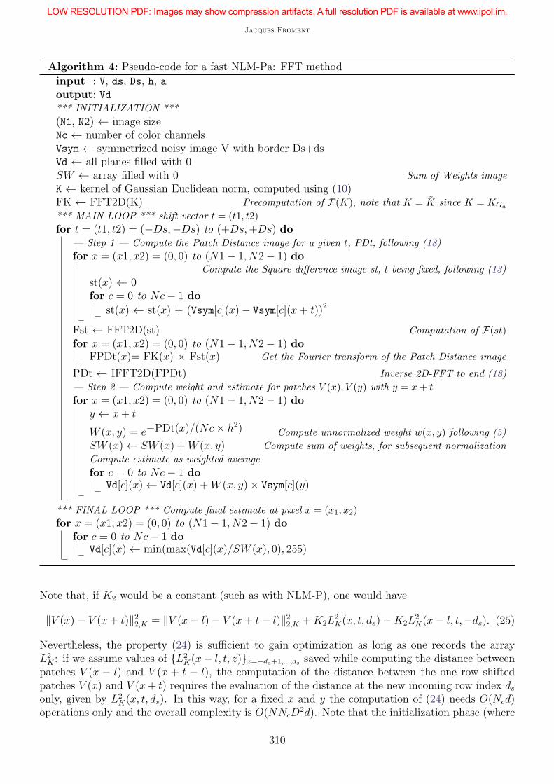
Algorithm 4: Pseudo-code for a fast NLM-Pa: FFT method


(N1, N2) ← image sizeNc ← number of color channelsVsym ← symmetrized noisy image V with border Ds+dsVd ← all planes filled with 0SW ← array filled with 0 Sum of Weights image

K ← kernel of Gaussian Euclidean norm, computed using (10)FK ← FFT2D(K) Precomputation of F(K), note that K = K since K = KGa

*** MAIN LOOP *** shift vector t = (t1, t2)

for t = (t1, t2) = (−Ds,−Ds) to (+Ds,+Ds) do— Step 1 — Compute the Patch Distance image for a given t, PDt, following (18)

for x = (x1, x2) = (0, 0) to (N1− 1, N2− 1) doCompute the Square difference image st, t being fixed, following (13)

st(x) ← 0for c = 0 to Nc− 1 do

st(x) ← st(x) + (Vsym[c](x)− Vsym[c](x+ t))2

Fst ← FFT2D(st) Computation of F(st)

for x = (x1, x2) = (0, 0) to (N1− 1, N2− 1) doFPDt(x)= FK(x) × Fst(x) Get the Fourier transform of the Patch Distance image

PDt ← IFFT2D(FPDt) Inverse 2D-FFT to end (18)

— Step 2 — Compute weight and estimate for patches V (x), V (y) with y = x+ t

for x = (x1, x2) = (0, 0) to (N1− 1, N2− 1) doy ← x+ t

W (x, y) = e−PDt(x)/(Nc× h2) Compute unnormalized weight w(x, y) following (5)

SW (x)← SW (x) +W (x, y) Compute sum of weights, for subsequent normalization

Compute estimate as weighted average

for c = 0 to Nc− 1 doVd[c](x)← Vd[c](x) +W (x, y)× Vsym[c](y)

*** FINAL LOOP *** Compute final estimate at pixel x = (x1, x2)

for x = (x1, x2) = (0, 0) to (N1− 1, N2− 1) dofor c = 0 to Nc− 1 do

Vd[c](x)← min(max(Vd[c](x)/SW (x), 0), 255)

Note that, if K2 would be a constant (such as with NLM-P), one would have

‖V (x)− V (x+ t)‖22,K = ‖V (x− l)− V (x+ t− l)‖22,K +K2L2K(x, t, ds)−K2L

2K(x− l, t,−ds). (25)

Nevertheless, the property (24) is sufficient to gain optimization as long as one records the arrayL2K : if we assume values of L2

K(x− l, t, z)z=−ds+1,...,ds saved while computing the distance betweenpatches V (x − l) and V (x + t − l), the computation of the distance between the one row shiftedpatches V (x) and V (x+ t) requires the evaluation of the distance at the new incoming row index dsonly, given by L2

K(x, t, ds). In this way, for a fixed x and y the computation of (24) needs O(Ncd)operations only and the overall complexity is O(NNcD

2d). Note that the initialization phase (where

310


one calculates the distance between the first patches) involves computing all values of the L2K array,

leading to a complexity of O(Ncd2). However this situation occurs only once, or to simplify the

implementation only once per image column, so as long as N2 > d the initialization process has acomplexity bounded by O(NNcD

2d).A pseudo-code for this fast NLM-Pa is proposed in Algorithm 5 and more detail on the imple-

mentation is given in Subsection 5.2. Note that the chosen pseudo-code and implementation resultfrom a compromise between efficiency and simplicity: by avoiding the initialization phase when xmoves to the next column by implementing a sum of shifted invariant columns, one would obtain afaster code (but without changing the overall complexity of O(NNcD

2d)); by adapting the scan ofx and y pixels so that the iteration next to x and y would be x+ l and y + l, one would reduce thememory size needed to record the L2

K array.

4 Experiments on Databases: Parameters Estimation and

Experimental Results

Having fast implementations, the NLM usability is now determined by the ability to set its 3 (NLM-P) or 4 (NLM-Pa) parameters in order to obtain an effective denoising. Methods that propose toautomatically adjust NLM parameters according to local or global characteristics of the image willnot be considered here, insofar as they lead to algorithms that differ from the original NLM. Thereader interested in such NLM extensions may consult [15, 9] and references therein. To estimateNLM parameters, the optimal values are calculated from a set of noise-free natural images on whichis added on each plane a Gaussian noise with mean 0 and given standard deviation, so that inputimages may be deemed to satisfy the noisy image model (1) with a known σ.

4.1 Parameters Estimation Using Two Image Databases

To build the image database, the choice was to take the 21 color images proposed in the on-linedemo of the IPOL article [4]. These images are assumed to be almost free of noise, as they have beenobtained by taking a good quality photograph in broad daylight and they have been post-processedwith a low-pass filter followed by a sub-sampling of factor 8. These color images contain 3 color planesin the RGB color model, each channel being coded using 8 bits. In the following, the correspondingdatabase will be called Color IPOL.

Since the patch distances (11) and (9) are computed using all color components, the estimationof the oracle |u(x) − u(y)| will be more reliable as the number of channels Nc increases. Therefore,parameter’s values (especially the patch side length d) should depend on the number of channels.To assess this effect, another database made of gray-level images (one 8-bits channel) is used. Suchimages are simply the grayed version of Color IPOL ones, using the Rec. 601 Luma weights3. Theresulting database will be called Gray-level IPOL.

From any of these two databases, the procedure used to get optimal parameters is as follows. Thestandard deviation is quantified between 1 and 100 with a step of one. Gaussian noise with mean0 and standard deviation σ ∈ [[1, 100]] is added to each image in the database, using the MersenneTwister pseudo-random number generator provided by IPOL development tools4. In order to limitthe impact of the noise realization, 10 noisy images per noise-free image are generated. This resultsin 210 different noisy images per database that are used as input of the optimization process. Thefunction fσ to be maximized is the arithmetic mean of the Peak Signal to Noise Ratio (PSNR)

3http://en.wikipedia.org/wiki/Luma_%28video%29.4https://tools.ipol.im/wiki/doc/tools.

311

http://en.wikipedia.org/wiki/Luma_%28video%29

https://tools.ipol.im/wiki/doc/tools

Jacques Froment

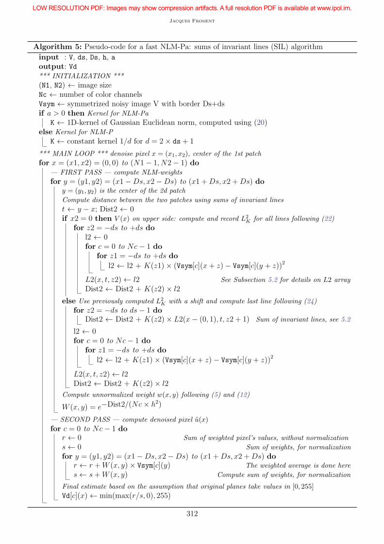
Algorithm 5: Pseudo-code for a fast NLM-Pa: sums of invariant lines (SIL) algorithm


(N1, N2) ← image sizeNc ← number of color channelsVsym ← symmetrized noisy image V with border Ds+dsif a > 0 then Kernel for NLM-Pa

K ← 1D-kernel of Gaussian Euclidean norm, computed using (20)else Kernel for NLM-P

K ← constant kernel 1/d for d = 2× ds+ 1




Compute distance between the two patches using sums of invariant lines

t ← y − x; Dist2 ← 0if x2 = 0 then V (x) on upper side: compute and record L2

K for all lines following (22)

for z2 = −ds to +ds dol2 ← 0for c = 0 to Nc− 1 do

for z1 = −ds to +ds do

l2 ← l2 + K(z1)× (Vsym[c](x+ z)− Vsym[c](y + z))2

L2(x, t, z2)← l2 See Subsection 5.2 for details on L2 array

Dist2 ← Dist2 + K(z2)× l2

else Use previously computed L2K with a shift and compute last line following (24)

for z2 = −ds to ds− 1 doDist2 ← Dist2 + K(z2)× L2(x− (0, 1), t, z2 + 1) Sum of invariant lines, see 5.2

l2 ← 0for c = 0 to Nc− 1 do

for z1 = −ds to +ds do

l2 ← l2 + K(z1)× (Vsym[c](x+ z)− Vsym[c](y + z))2

L2(x, t, z2)← l2Dist2 ← Dist2 + K(z2)× l2

Compute unnormalized weight w(x, y) following (5) and (12)








Vd[c](x)← min(max(r/s, 0), 255)

312


between each noisy image and its noise-free version and the optimization problem may be written,in the case of the NLM-Pa denoising scheme and for B the image database,

fNLM-Pa,Bσ (d⋆s, D

⋆s , h

⋆, a⋆) = maxds,Ds,h,a

1

10|B|

∑

u∈B

10∑

i=1

PSNR(u, uNLM-Pa(u, i, σ, ds, Ds, h, a))

, (26)

where uNLM-Pa(u, i, σ, ds, Ds, h, a) is the denoised image computed from the noisy input u + ǫi (ǫibetween a noise realization of standard deviation σ), using NLM-Pa algorithm with parametersds, Ds, h, a. The same writing is obtained for fNLM-P,B

σ , without the last parameter a.Since the complexity of fσ does not allow the use of conventional optimization algorithms, the only

safe method is to discretize the parameters and try as many combinations as possible. Fortunately,parameters ds and Ds are integers and they can reasonably be limited to small bounds. As mentionedin the literature (see e.g. [1, 4]), the parameter h that controls the decay of the weights should beproportional to the value of σ and in practice, a value of h slightly greater than σ seems to be thebest. The literature provides little guidance on the choice of the parameter a. In [11] (nlmeansmodule), the default value a = ds/2 is proposed. Based on these considerations, Table 2 gives thequantized values and their bounds that have been used for the parameter exploration. Exploringall of these parameters would require 329120 calls to the NLM-Pa code for a given input image andstandard deviation, so the parameters estimation for the Color or the Gray-level IPOL databasewould need more than 6.9 × 109 calls. Knowing that a call typically lasts a few seconds, it wouldnot be possible to explore all the 329120 parameters combination. To reduce the dimensionality ofthe problem, a local optimum is sought with the following coordinate ascent algorithm where onecyclically iterates through each parameter direction:

dk+1s = argmax

dsfNLM-Pa,Bσ (ds, D

ks , h

k, ak)

Dk+1s = argmax

Ds

fNLM-Pa,Bσ (dk+1

s , Ds, hk, ak)

hk+1 = argmaxh

fNLM-Pa,Bσ (dk+1

s , Dk+1s , h, ak)

ak+1 = argmaxa

fNLM-Pa,Bσ (dk+1

s , Dk+1s , hk+1, a),

(27)

where k is the current iteration. The algorithm stops when a stationary point is reached, i.e. whenthere is no improvement in the last cycle. In practice it appears that a stationary point is reachedvery rapidly, typically in 3 to 5 iterations. The results are given in Table 3 (NLMP-a) and Table 4(NLM-P), where optimal values are piecewise-constant interpolated for non-integer values of σ (whenthe expression does not show the σ term).

Parameter Meaning Quantized as integer Rangeds patch side half-length ds ds ∈ [[1, 11]]Ds search window side half-length Ds Ds ∈ [[1, 17]]h = σhQ/10 filtering parameter, see (5) and (12) hQ hQ ∈ [[5, 20]]a = aQ/10 decay of the Gaussian kernel (10) aQ aQ ∈ [[1, 110]]

Table 2: Range of the NLM-P and NLM-Pa parameter exploration for the optimization process.

4.2 Experimental Results and Comparison With Blockwise NLM (NLM-B)

This subsection presents experimental results on NLM-P and NLM-Pa with previously computedoptimal parameters, together with results obtained with the blockwise NLM (NLM-B) [1] (Section

313

Jacques Froment

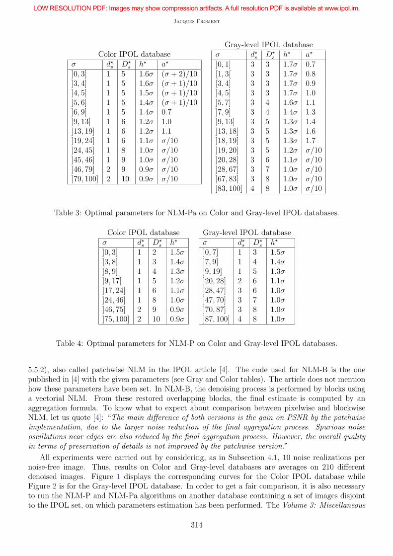
Color IPOL databaseσ d⋆s D⋆

s h⋆ a⋆

]0, 3] 1 5 1.6σ (σ + 2)/10]3, 4] 1 5 1.6σ (σ + 1)/10]4, 5] 1 5 1.5σ (σ + 1)/10]5, 6] 1 5 1.4σ (σ + 1)/10]6, 9] 1 5 1.4σ 0.7]9, 13] 1 6 1.2σ 1.0]13, 19] 1 6 1.2σ 1.1]19, 24] 1 6 1.1σ σ/10]24, 45] 1 8 1.0σ σ/10]45, 46] 1 9 1.0σ σ/10]46, 79] 2 9 0.9σ σ/10]79, 100] 2 10 0.9σ σ/10

Gray-level IPOL databaseσ d⋆s D⋆

s h⋆ a⋆

]0, 1] 3 3 1.7σ 0.7[1, 3[ 3 3 1.7σ 0.8[3, 4] 3 3 1.7σ 0.9]4, 5] 3 3 1.7σ 1.0]5, 7] 3 4 1.6σ 1.1]7, 9] 3 4 1.4σ 1.3]9, 13] 3 5 1.3σ 1.4]13, 18] 3 5 1.3σ 1.6]18, 19] 3 5 1.3σ 1.7]19, 20] 3 5 1.2σ σ/10]20, 28] 3 6 1.1σ σ/10]28, 67] 3 7 1.0σ σ/10]67, 83] 3 8 1.0σ σ/10]83, 100] 4 8 1.0σ σ/10

Table 3: Optimal parameters for NLM-Pa on Color and Gray-level IPOL databases.

Color IPOL databaseσ d⋆s D⋆

s h⋆

]0, 3] 1 2 1.5σ]3, 8] 1 3 1.4σ]8, 9] 1 4 1.3σ]9, 17] 1 5 1.2σ]17, 24] 1 6 1.1σ]24, 46] 1 8 1.0σ]46, 75] 2 9 0.9σ]75, 100] 2 10 0.9σ

Gray-level IPOL databaseσ d⋆s D⋆

s h⋆

]0, 7] 1 3 1.5σ]7, 9] 1 4 1.4σ]9, 19] 1 5 1.3σ]20, 28] 2 6 1.1σ]28, 47] 3 6 1.0σ]47, 70] 3 7 1.0σ]70, 87] 3 8 1.0σ]87, 100] 4 8 1.0σ

Table 4: Optimal parameters for NLM-P on Color and Gray-level IPOL databases.

5.5.2), also called patchwise NLM in the IPOL article [4]. The code used for NLM-B is the onepublished in [4] with the given parameters (see Gray and Color tables). The article does not mentionhow these parameters have been set. In NLM-B, the denoising process is performed by blocks usinga vectorial NLM. From these restored overlapping blocks, the final estimate is computed by anaggregation formula. To know what to expect about comparison between pixelwise and blockwiseNLM, let us quote [4]: “The main difference of both versions is the gain on PSNR by the patchwiseimplementation, due to the larger noise reduction of the final aggregation process. Spurious noiseoscillations near edges are also reduced by the final aggregation process. However, the overall qualityin terms of preservation of details is not improved by the patchwise version.”

All experiments were carried out by considering, as in Subsection 4.1, 10 noise realizations pernoise-free image. Thus, results on Color and Gray-level databases are averages on 210 differentdenoised images. Figure 1 displays the corresponding curves for the Color IPOL database whileFigure 2 is for the Gray-level IPOL database. In order to get a fair comparison, it is also necessaryto run the NLM-P and NLM-Pa algorithms on another database containing a set of images disjointto the IPOL set, on which parameters estimation has been performed. The Volume 3: Miscellaneous

314


set from the USC-SIPI Image Database [26] has been chosen because it includes some standard testimages, such as House (record ID 4.1.05), Mandrill (4.2.03) and Lena (4.2.04). In what follows, theMiscellaneous Volume of the USC-SIPI Image Database is shortened by USC-SIPI. It contains 44images (16 color and 28 monochrome) of very different nature and far away from the IPOL set, suchas old photographs and test patterns. The PSNR curves (average on 440 denoised images) for theUSC-SIPI database is given in Figure 3.

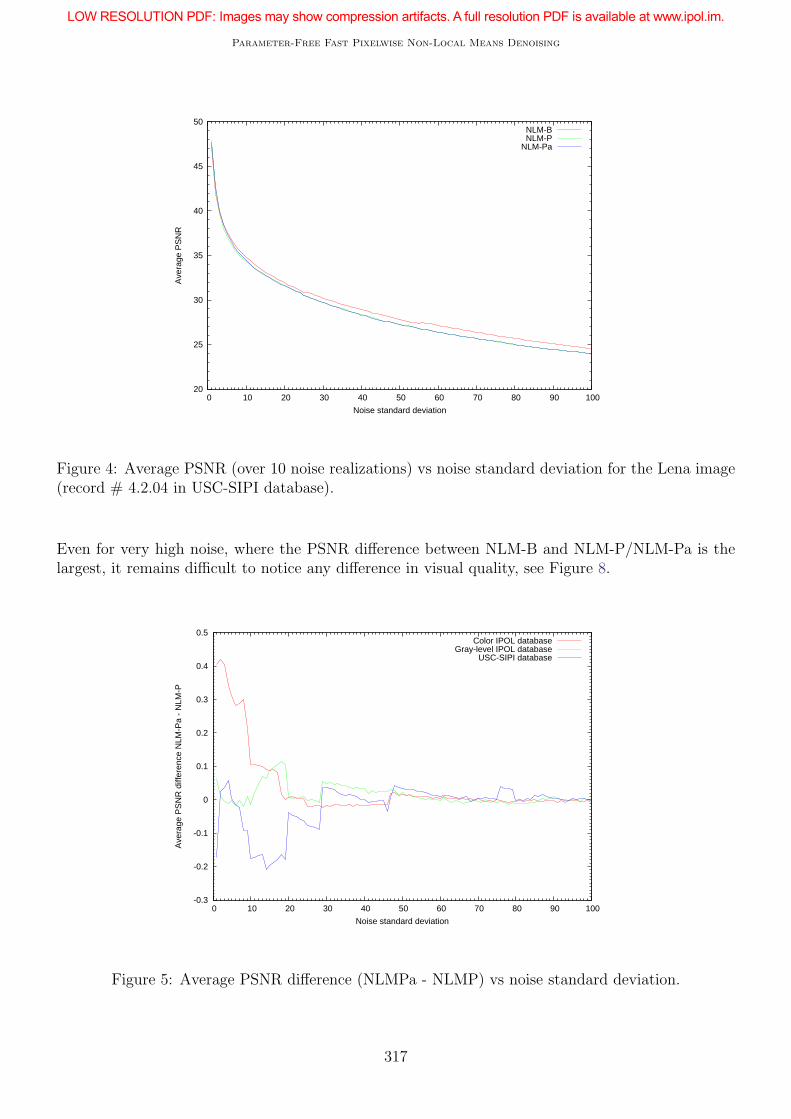
It is remarkable that PSNR curves on the USC-SIPI database are very similar to the ones withIPOL databases. This indicates that the computed optimal parameters are robust to image variation.Another indication confirming the relevance of these optimal parameters is in the convex and regularshape of the NLM-P and NLM-Pa curves. In contrast, the few irregularities that can be noted inNLM-B curves suggest that the parameters given in [4] are suboptimal in some standard deviationintervals, with respect to the PSNR criterion. One reason of the curves regularity is in the largePSNR averaging done on images of the database. However the curves regularity remains quite goodon a single image, see Figure 4 where are plotted PSNR curves for the standard Lena image (record# 4.2.04 in the USC-SIPI database; remember that this image is not in the database used to computeoptimal NLM-P and NLM-Pa parameters).

20

25

30

35

40

45

50

0 10 20 30 40 50 60 70 80 90 100

Ave

rage

PS

NR

Noise standard deviation

NLM-BNLM-P

NLM-Pa

Figure 1: Average PSNR vs noise standard deviation for Color IPOL database.

Let us now compare the performance of the three denoising methods. The experiments confirmthat the Gaussian Euclidean patch distance (9) does not bring much compared to the Euclideanone (11), see Figure 5 where average PSNR differences between NLM-Pa and NLM-P are drawn.The difference between NLM-B and NLM-Pa is plotted in Figure 6. In agreement with the textfrom [4] quoted above, NLM-B presents better PSNR than NLM-P/NLM-Pa when the noise standarddeviation is greater than 3 (USC-SIPI), 5 (Color IPOL) or 15 (Gray-level IPOL). As expected thevisual quality of the images is so similar that it is hard to notice any difference, see Figure 7 where thenoise standard deviation is 20. At most we can remark that the NLM-P/NLM-Pa restored imagesappear a little bit more blurry that the NLM-B. By cons, a bit of plum on the back of the hatdisappeared on the NLM-B denoised image while it is still discernible on NLM-P/NLM-Pa ones.

315

Jacques Froment

20

25

30

35

40

45

50

0 10 20 30 40 50 60 70 80 90 100

Ave

rage

PS

NR


NLM-BNLM-P

NLM-Pa

Figure 2: Average PSNR vs noise standard deviation for Gray-level IPOL database.

20

25

30

35

40

45

50

0 10 20 30 40 50 60 70 80 90 100

Ave

rage

PS

NR


NLM-BNLM-P

NLM-Pa

Figure 3: Average PSNR vs noise standard deviation for USC-SIPI database.

316


20

25

30

35

40

45

50

0 10 20 30 40 50 60 70 80 90 100

Ave

rage

PS

NR


NLM-BNLM-P

NLM-Pa

Figure 4: Average PSNR (over 10 noise realizations) vs noise standard deviation for the Lena image(record # 4.2.04 in USC-SIPI database).

Even for very high noise, where the PSNR difference between NLM-B and NLM-P/NLM-Pa is thelargest, it remains difficult to notice any difference in visual quality, see Figure 8.

-0.3

-0.2

-0.1

0

0.1

0.2

0.3

0.4

0.5

0 10 20 30 40 50 60 70 80 90 100

Ave

rage

PS

NR

diff

eren

ce N

LM-P

a -

NLM

-P


Color IPOL databaseGray-level IPOL database

USC-SIPI database

Figure 5: Average PSNR difference (NLMPa - NLMP) vs noise standard deviation.

317

Jacques Froment

-0.6

-0.4

-0.2

0

0.2

0.4

0.6

0.8

1

0 10 20 30 40 50 60 70 80 90 100

Ave

rage

PS

NR

diff

eren

ce N

LM-B

- N

LM-P

a



USC-SIPI database

Figure 6: Average PSNR difference (NLM-B - NLMPa) vs noise standard deviation.

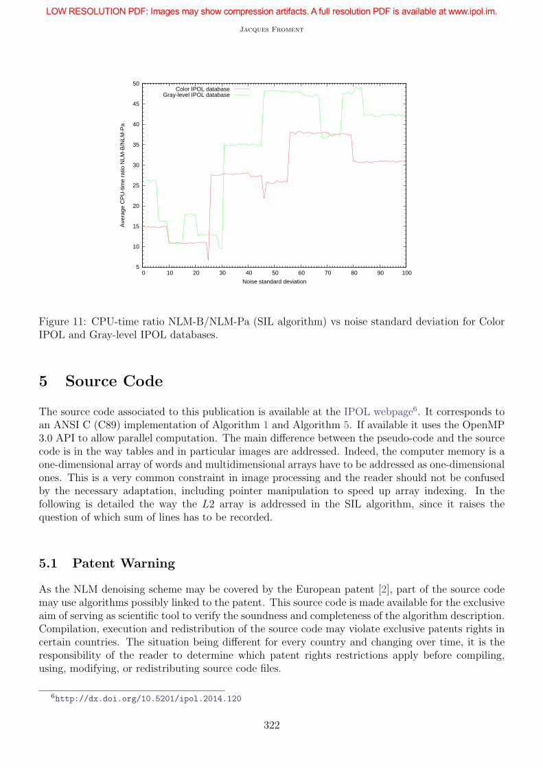
In order to compare the speed of NLM-B, NLM-P and NLM-Pa, we consider the total amountof CPU-time5 spent by the denoising process alone (therefore excluding input/output to read andwrite images on disk as well as the generation of the noisy image). Note that this CPU-time doesnot represent the elapsed real time (wall clock) taken from the start of the process until the end: asall algorithms are implemented using parallel processing, on a multi-core computer the elapsed realtime would be approximately the CPU-time divided by the number of used CPU (provided that noother program is running at the same time). Figure 9 gives the CPU-time spent on average on theColor IPOL database while Figure 10 is for the Gray-level IPOL database. Figure 11 displays theratio of the CPU-time between NLM-B and NLM-Pa with the SIL algorithm. We first remark thaton the Color IPOL database, the SIL algorithm is faster than the basic one in case of high noise only.The reason is simply in the optimum value of d⋆s = 1 for σ ≤ 46: for such a tiny patch it is uselessto develop fast patch distance computation. The situation differs for NLM-Pa with grayscale imageswhere d⋆s ≥ 3. Nevertheless, the increase in speed of the SIL algorithm compared to the basic onenever exceeds the factor 4.5. However it should be noted that the speed increase may be much moreimportant for NLM variants where the recommended patch size is greater than the maximum value ofd⋆s = 4 obtained here, see for example [14]. In the experiments the NLM-B algorithm appears muchslower than NLM-P/NLM-Pa, with a CPU-time ratio between 6 (Color IPOL database, σ = 25)and 49 (Gray-level IPOL database, σ = 83). This may seem surprising in view of [1] (Section 5.5.2)where the blockwise NLM version is presented as a way to reduce the complexity of the pixelwiseNLM. The reason is in the block overlapping that is not lowered in the NLM-B implementation [4]:using fewer blocks in the aggregation procedure would reduce the computation time, but probablyalso the denoising performance. Another element to explain the difference in speed between NLM-Band NLM-P/NLM-Pa is in the search window size, given by the parameter Ds. In the textbook case

5See http://www.gnu.org/software/libc/manual/html_node/CPU-Time.html. Processors used to perform theexperiments were Intel Xeon L5640. All programs were compiled with OpenMP multithreading and all compileroptimizations turned on.

318

http://www.gnu.org/software/libc/manual/html_node/CPU-Time.html


Figure 7: Visual comparison of parameter-free denoising algorithms applied on Lena image (σ = 20;zoom on a part but PSNRs are computed on the whole image; in this experiment the noise realizationis the same for all of the three denoising algorithms). From left to right and top to bottom: originalu; NLM-B (PSNR=31.90); NLM-P (PSNR=31.61); NLM-Pa (PSNR=31.61).

where σ = 20 and for the Gray-level IPOL database, the speed ratio reaches almost 18 while the patchsize is larger for NLM-Pa (d⋆s = 3 corresponds to a patch size of 7× 7) than for NLM-B (patch sizeof 3× 3). On the other hand, the search window size is only 11× 11 for NLM-Pa where it is 21× 21for NLM-B. In fact, whatever the database and the noise standard deviation, the optimal searchwindow size for NLM-P and NLM-Pa is always less than or equal to the one of NLM-B. Though onecan not compare them precisely (the algorithms being slightly different), this small optimal size is

319

Jacques Froment

Figure 8: Visual comparison of parameter-free denoising algorithms applied on Lena image (σ = 60;zoom on a part but PSNRs are computed on the whole image; in this experiment the noise realizationis the same for all of the three denoising algorithms). From left to right and top to bottom: originalu; NLM-B (PSNR=27.18); NLM-P (PSNR=26.43); NLM-Pa (PSNR=26.43).

consistent with that given in [19] and the study confirms the common overestimation of the searchwindow size. One may hope that the proposed fast pixelwise NLM implementation combined withoptimal parameters giving a reasonable search window size will contribute to reconsider the originalNLM scheme, usually considered as a slow denoising method.

320


0

50

100

150

200

250

300

350

400

0 10 20 30 40 50 60 70 80 90 100

Ave

rage

tota

l num

ber

of C

PU

-sec

onds

use

d by

the

proc

ess


NLM-BNLM-P (SIL algorithm)

NLM-Pa (SIL algorithm)NLM-Pa (basic algorithm)

Figure 9: Total amount of CPU-time used by the denoising processes vs noise standard deviation:average over the Color IPOL database.

0

50

100

150

200

250

300

350

0 10 20 30 40 50 60 70 80 90 100

Ave

rage

tota

l num

ber

of C

PU

-sec

onds

use

d by

the

proc

ess


NLM-BNLM-P (SIL algorithm)

NLM-Pa (SIL algorithm)NLM-Pa (basic algorithm)

Figure 10: Total amount of CPU-time used by the denoising processes vs noise standard deviation:average over the Gray-level IPOL database.

321

Jacques Froment

5

10

15

20

25

30

35

40

45

50

0 10 20 30 40 50 60 70 80 90 100

Ave

rage

CP

U-t

ime

ratio

NLM

-B/N

LM-P

a



Figure 11: CPU-time ratio NLM-B/NLM-Pa (SIL algorithm) vs noise standard deviation for ColorIPOL and Gray-level IPOL databases.

5 Source Code

The source code associated to this publication is available at the IPOL webpage6. It corresponds toan ANSI C (C89) implementation of Algorithm 1 and Algorithm 5. If available it uses the OpenMP3.0 API to allow parallel computation. The main difference between the pseudo-code and the sourcecode is in the way tables and in particular images are addressed. Indeed, the computer memory is aone-dimensional array of words and multidimensional arrays have to be addressed as one-dimensionalones. This is a very common constraint in image processing and the reader should not be confusedby the necessary adaptation, including pointer manipulation to speed up array indexing. In thefollowing is detailed the way the L2 array is addressed in the SIL algorithm, since it raises thequestion of which sum of lines has to be recorded.

5.1 Patent Warning

As the NLM denoising scheme may be covered by the European patent [2], part of the source codemay use algorithms possibly linked to the patent. This source code is made available for the exclusiveaim of serving as scientific tool to verify the soundness and completeness of the algorithm description.Compilation, execution and redistribution of the source code may violate exclusive patents rights incertain countries. The situation being different for every country and changing over time, it is theresponsibility of the reader to determine which patent rights restrictions apply before compiling,using, modifying, or redistributing source code files.

6http://dx.doi.org/10.5201/ipol.2014.120

322




5.2 Implementation of Fast NLM-Pa Using Sums of Invariant Lines

The pseudo-code of Algorithm 5 does not show how is managed the L2 array that records weightedquadratic distances between patches V (x) and V (x + t), denoted by L2

K(x, t, z2). Two points areimportant to understand the chosen implementation: which samples are recorded in L2 and how theshift is performed along the line axis.

• The main loop is on pixels x = (x1, x2) ∈ Ω to be denoised and these pixels are scanned fromtop to bottom and left to right, so that the inner loop on line x2 is done after the inner loopon column x1. Thus, except when the pixel x is on the first line of the image (x2 = 0 case), itspredecessor in the scan is x − (0, 1). Inside the main loop, values of L2

K(x, t, z2) have to berecorded for y = x + t ∈ Ωx and z2 ∈ [[−ds,+ds]] and one gets D2d samples. Computation ofthese values requires knowledge of L2

K(x − (0, 1), t, z2) for y = x − (0, 1) + t ∈ Ωx−(0,1) andz2 ∈ [[−ds,+ds]] and they were those that were calculated at the previous iteration x − (0, 1).Thus, only the parity of x2 has to be indexed and the size of the L2 array is then of 2D2dsamples. The correspondence between L2 values and L2

K function values is the following:L2K(x, t, z2) = L2[(x2%2)×D2 × d+ (y2 − x2 +Ds)×D × d+ (y1 − x1 +Ds)× d+ z2] where

% is the integer modulo operator. Note that y is not indexed by its absolute position in theplane Ω but by its relative position t+ (Ds, Ds) with respect to x.

• Looking more closely at how previously computed values of L2 at x−(0, 1) are used to computevalues at x, equations (23) and (24) tell us that a shift of one z2-line down has to be performedon the L2 array when one goes from a pixel x to the next, for the same relative position of y.This can be easily done during the sum of invariant lines by updating the L2 array followingEquation (23) that can be written in pseudo-code

L2K(x, t, z2)← L2

K(x− l, t, z2 + 1). (28)

5.3 Lookup Table for Fast Computation of Exponential Function

Calculation of NLM-weights (12) and (5) from patches distance uses the computationally intensiveexponential function x ∈ R

+ 7→ e−x. As it is not essential to get the NLM-weights with a highaccuracy, one may accelerate the code using a Look-Up-Table (LUT). This LUT is an array thatholds a set of precomputed values (e−xn)n, where the (xn)n are uniformly sampled. When a particularvalue of e−x is wanted, the two closest values e−xn and e−xn+1 (xn ≤ x ≤ xn+1) recorded in the LUTare read to estimate e−x, using a linear interpolation. Such a LUT is part of the C++ code publishedin [4] to implement NLM-B and it is also used in the present C code to implement NLM-P/NLM-Pa.The precision of the estimation is given by the sampling period (that is, by the interval between twoadjacent samples) and it has been tuned so that denoised images in the PNG output format (seebelow) would be identical, when using the original exponential function or the estimation with theLUT.

5.4 How Experiments Were Performed

The experiments reported in Section 4 were conducted using the reviewed C code as well as theC++ code published in [4], without any modification but the inclusion of functions needed to getand print the CPU-time. The optimization process and the presentation of results have requiredsome additional code, written in Bash scripts7 that are not included into this publication. As

7http://en.wikipedia.org/wiki/Bash_%28Unix_shell%29.

323

http://en.wikipedia.org/wiki/Bash_%28Unix_shell%29

Jacques Froment

the input/output images of the C and C++ codes are in PNG format8, PSNR are computed onimages with channel’s values being integers (between 0 and 255) even though the denoising algorithmproduces images with floating-point values. Therefore, results may slightly differ if simulations areredone by bypassing the PNG format. The alternative of a PSNR computation done before channel’svalues thresholding would have led to a result that does not accurately reflects the observed images.

6 Online Demo

An online demo running the source code is available at the IPOL webpage9, with an interface similarto that of the NLM-B demo [4].

Inputs are the noise-free image u (a grayscale or a 3-planes color image) and the standard deviationσ of the added noise. The user may upload its own image or may choose any of the available imageson the demo page. The algorithm may be applied on a subpart of the image, by clicking on twoopposite corners in the displayed image. In order to keep a simple interface, the demo does not allowto pass options to the program. Therefore, the applied algorithm is always NLM-Pa with the SILimplementation (Algorithm 5). Outputs are the noisy image v and the denoised one u. The PSNRas well as the RMSE (Root-Mean-Square Error) between u and u are displayed.

The user who wishes to select options, for example to run NLM-P or the basic implementation(Algorithm 1), should compile the source code (see Section 5) and run the program from its owncomputer.

Acknowledgments

I thank the IRISA-UBS research center for allowing me access to their computer cluster partiallyfunded by the CPER Invent’IST masse de donnees with the following partners: the French Ministryof Research, the Brittany Region, the General Council of Morbihan and the European RegionalDevelopment Fund.

Image Credits

Standard test image (record # 4.2.04 in USC-SIPI image database [26]). In figures 7 and 8 the cropping

(200, 200)− (299, 299) has been performed.

References

[1] A. Buades, B. Coll, and J.M. Morel, A review of image denoising algorithms, with a newone, Multiscale Modeling & Simulation, 4 (2005), pp. 490–530. http://dx.doi.org/10.1137/040616024.

[2] , Image data processing method by reducing image noise, and camera integrating means forimplementing said method. ED Patent 1,749,278, February 2007.

[3] , Image denoising methods. A new nonlocal principle, Siam Review, 52 (1) (2010), pp. 113–147. http://dx.doi.org/10.1137/090773908.

8http://en.wikipedia.org/wiki/Portable_Network_Graphics.9http://dx.doi.org/10.5201/ipol.2014.120

324


http://dx.doi.org/10.1137/040616024

http://dx.doi.org/10.1137/040616024

http://dx.doi.org/10.1137/090773908

http://en.wikipedia.org/wiki/Portable_Network_Graphics



[4] , Non-local means denoising, Image Processing On Line, (2011). http://dx.doi.org/10.5201/ipol.2011.bcm_nlm.

[5] P. Coupe, P. Yger, and C. Barillot, Fast non local means denoising for 3D MR images, inMedical Image Computing and Computer-Assisted Intervention–MICCAI 2006, Springer, 2006,pp. 33–40. http://dx.doi.org/10.1007/11866763_5.

[6] F.C. Crow, Summed-area tables for texture mapping, ACM SIGGRAPH Computer Graphics,18 (1984), pp. 207–212. http://dx.doi.org/10.1145/800031.808600.

[7] J. Darbon, A. Cunha, T.F. Chan, S. Osher, and G.J. Jensen, Fast nonlocal filtering ap-plied to electron cryomicroscopy, in 5th IEEE International Symposium on Biomedical Imaging:From Nano to Macro, 2008, pp. 1331–1334. http://dx.doi.org/10.1109/ISBI.2008.4541250.

[8] C.A. Deledalle, V. Duval, and J. Salmon, Non-local methods with shape-adaptive patches(NLM-SAP), Journal of Mathematical Imaging and Vision, 43 (2012), pp. 103–120. http:

//dx.doi.org/10.1007/s10851-011-0294-y.

[9] V. Duval, J.F. Aujol, and Y. Gousseau, A bias-variance approach for the non-local means,SIAM Journal on Imaging Sciences, 4 (2011), pp. 760–788. http://dx.doi.org/10.1137/

100790902.

[10] G. Facciolo, N. Limare, and E. Meinhardt, Integral images for block matching, ImageProcessing On Line, (2013). http://www.ipol.im/pub/pre/57/.

[11] J. Froment and L. Moisan (Eds), Megawave2 v.3.01. A free and open-source Uniximage processing software for reproducible research, available at http://megawave.cmla.

ens-cachan.fr, 2007.

[12] G. Gilboa and S. Osher, Nonlocal linear image regularization and supervised segmenta-tion, Multiscale Modeling & Simulation, 6 (2007), pp. 595–630. http://dx.doi.org/10.1137/060669358.

[13] S. Grewenig, S. Zimmer, and J. Weickert, Rotationally invariant similarity measuresfor nonlocal image denoising, Journal of Visual Communication and Image Representation, 22(2011), pp. 117–130. http://dx.doi.org/10.1016/j.jvcir.2010.11.001.

[14] Q. Jin, I. Grama, and Q. Liu, Removing gaussian noise by optimization of weights in non-local means. http://arxiv.org/abs/1109.5640, 2011.

[15] C. Kervrann and J. Boulanger, Optimal spatial adaptation for patch-based image denois-ing, IEEE Transactions On Image Processing, 15 (2006), pp. 2866–2878. http://dx.doi.org/10.1109/TIP.2006.877529.

[16] M. Lebrun, A. Buades, and J-M. Morel, Implementation of the ”Non-Local Bayes” (NL-Bayes) Image Denoising Algorithm, Image Processing On Line, 2013 (2013), pp. 1–42. http:

//dx.doi.org/10.5201/ipol.2013.16.

[17] M. Mahmoudi and G. Sapiro, Fast image and video denoising via nonlocal means of similarneighborhoods, IEEE Signal Processing Letters, 12 (2005), pp. 839–842. http://dx.doi.org/

10.1109/LSP.2005.859509.

325

http://dx.doi.org/10.5201/ipol.2011.bcm_nlm

http://dx.doi.org/10.5201/ipol.2011.bcm_nlm

http://dx.doi.org/10.1007/11866763_5

http://dx.doi.org/10.1145/800031.808600

http://dx.doi.org/10.1109/ISBI.2008.4541250

http://dx.doi.org/10.1007/s10851-011-0294-y

http://dx.doi.org/10.1007/s10851-011-0294-y

http://dx.doi.org/10.1137/100790902

http://dx.doi.org/10.1137/100790902

http://www.ipol.im/pub/pre/57/

http://megawave.cmla.ens-cachan.fr

http://megawave.cmla.ens-cachan.fr

http://dx.doi.org/10.1137/060669358

http://dx.doi.org/10.1137/060669358

http://dx.doi.org/10.1016/j.jvcir.2010.11.001

http://arxiv.org/abs/1109.5640

http://dx.doi.org/10.1109/TIP.2006.877529




http://dx.doi.org/10.1109/LSP.2005.859509


Jacques Froment

[18] C. Pang, O.C. Au, J. Dai, W. Yang, and F. Zou, A fast NL-means method in imagedenoising based on the similarity of spatially sampled pixels, in IEEE International Workshopon Multimedia Signal Processing, 2009, pp. 1–4. http://dx.doi.org/10.1109/MMSP.2009.

5293567.

[19] S. Postec, J. Froment, and B. Vedel, Non-local means est un algorithme de debruitagelocal (Non-local means is a local image denoising algorithm), in Proceedings of GRETSI, France,2013. http://arxiv.org/abs/1311.3768.

[20] B. Rajaei, An analysis and improvement of the BLS-GSM denoising method, Image ProcessingOn Line, 4 (2014), p. 4470. http://dx.doi.org/10.5201/ipol.2014.86.

[21] J. Salmon, On two parameters for denoising with non-local means, Signal Processing Letters,17 (2010), pp. 269–272. http://dx.doi.org/10.1109/LSP.2009.2038954.

[22] T. Tasdizen, Principal neighborhoods dictionaries for nonlocal means image denoising, IEEETransactions on Image Processing, 18 (2009), pp. 2649–2660. http://dx.doi.org/10.1109/

TIP.2009.2028259.

[23] R. Vignesh, B.T. Oh, and C-CJ Kuo, Fast non-local means (NLM) computation withprobabilistic early termination, IEEE Signal Processing Letters, 17 (2010), pp. 277–280. http://dx.doi.org/10.1109/LSP.2009.2038956.

[24] P. Viola and M. Jones, Rapid object detection using a boosted cascade of simple features,in Proceedings of the IEEE Computer Society Conference on Computer Vision and PatternRecognition, vol. 1, 2001, pp. I–511. http://dx.doi.org/10.1109/CVPR.2001.990517.

[25] J. Wang, Y. Guo, Y. Ying, Y. Liu, and Q. Peng, Fast non-local algorithm for imagedenoising, in IEEE International Conference on Image Processing, 2006, pp. 1429–1432. http://dx.doi.org/10.1109/ICIP.2006.312698.

[26] A.G Weber, The USC-SIPI image database version 5, tech. report, University of SouthernCalifornia, 1997. http://sipi.usc.edu/database.

[27] I. Wegener, Complexity Theory, exploring the limits of efficient algorithms, Springer, 2005.ISBN-13 978-3540210450.

326

http://dx.doi.org/10.1109/MMSP.2009.5293567

http://dx.doi.org/10.1109/MMSP.2009.5293567

http://arxiv.org/abs/1311.3768







http://dx.doi.org/10.1109/CVPR.2001.990517

http://dx.doi.org/10.1109/ICIP.2006.312698

http://dx.doi.org/10.1109/ICIP.2006.312698

http://sipi.usc.edu/database

Documents

Parameter-Free Fast Pixelwise Non-Local Means Denoising