Embed Size (px)
Citation preview
Marco F. Duarte
Parameter Estimation in Compressive Sensing
Systems of Lines: Application of Algebraic Combinatorics Worcester Polytechnic Institute, August 13 2015
x =�
n
�n�n = ��
x = ��
� = ��1
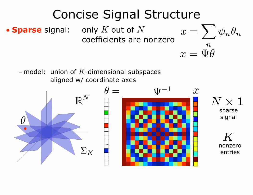
Concise Signal Structure
RN
sparsesignal
nonzero entries�K � �K
�
• Sparse signal: only K out of N coefficients are nonzero
–model: union of K-dimensional subspaces aligned w/ coordinate axes
x = ��
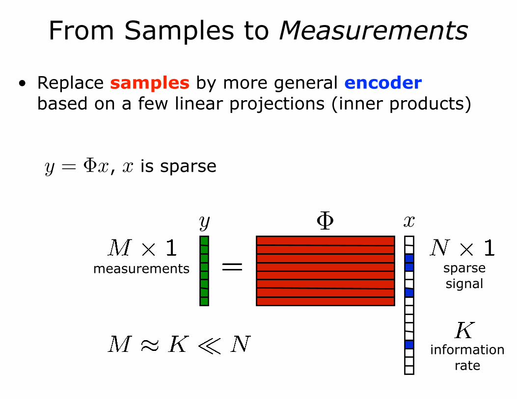
From Samples to Measurements
• Replace samples by more general encoder based on a few linear projections (inner products) , x is sparse
measurements sparsesignal
information rate
y x
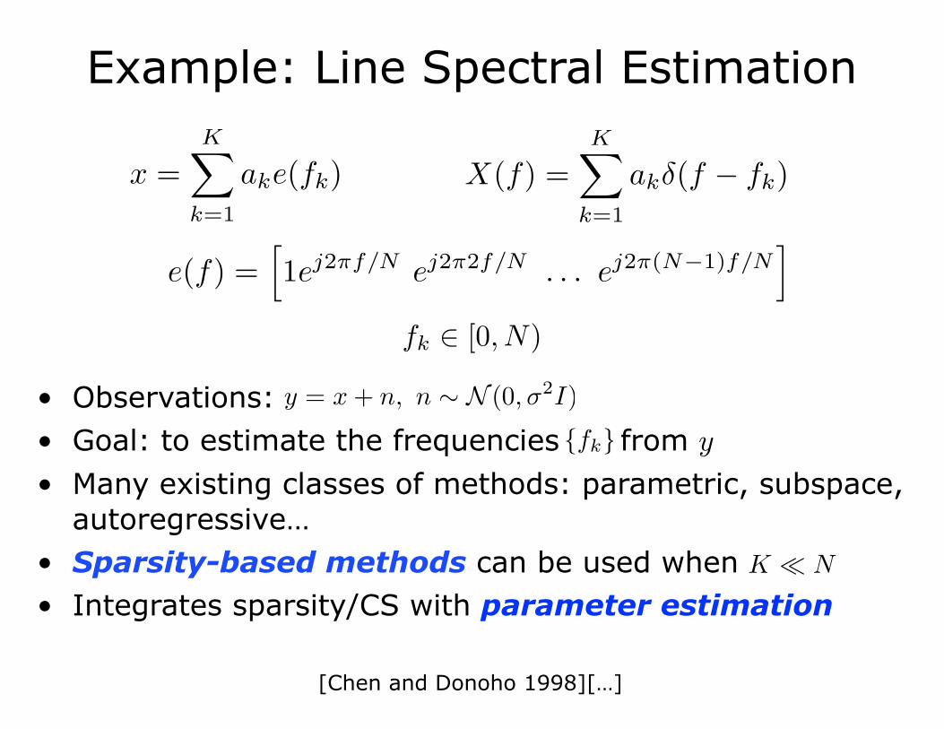
Example: Line Spectral Estimation
• Observations: • Goal: to estimate the frequencies from y • Many existing classes of methods: parametric, subspace,
autoregressive… • Sparsity-based methods can be used when • Integrates sparsity/CS with parameter estimation
[Chen and Donoho 1998][…]
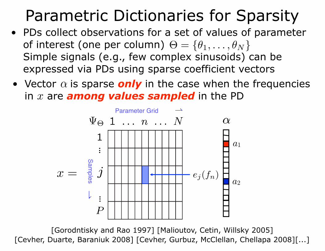
• PDs collect observations for a set of values of parameter of interest (one per column) Simple signals (e.g., few complex sinusoids) can be expressed via PDs using sparse coefficient vectors
• Vector is sparse only in the case when the frequencies in x are among values sampled in the PD
Parametric Dictionaries for Sparsity
[Gorodntisky and Rao 1997] [Malioutov, Cetin, Willsky 2005][Cevher, Duarte, Baraniuk 2008] [Cevher, Gurbuz, McClellan, Chellapa 2008][...]
Parameter Grid
Samples
a1
a2
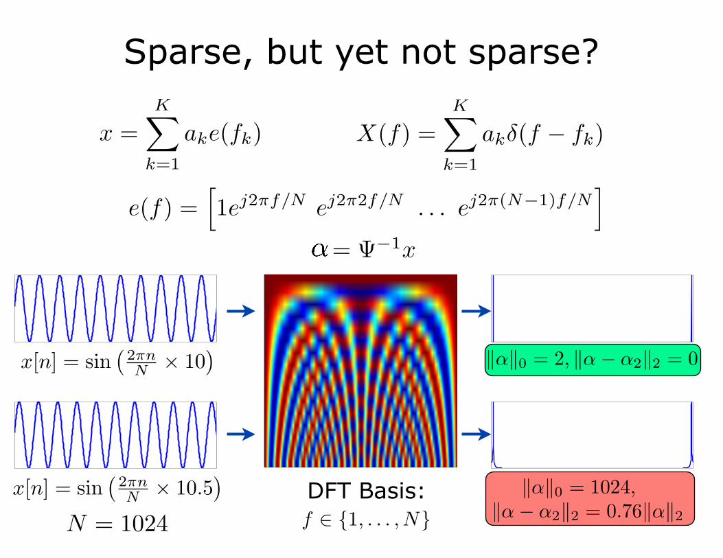
Sparse, but yet not sparse?
DFT Basis:
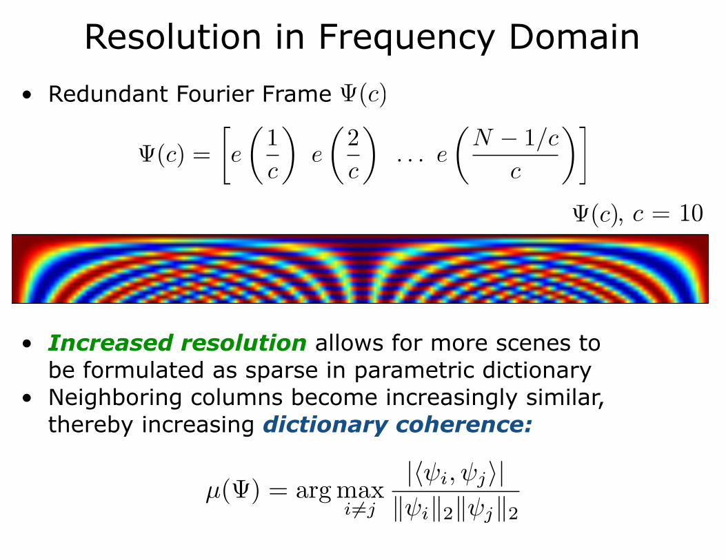
Resolution in Frequency Domain
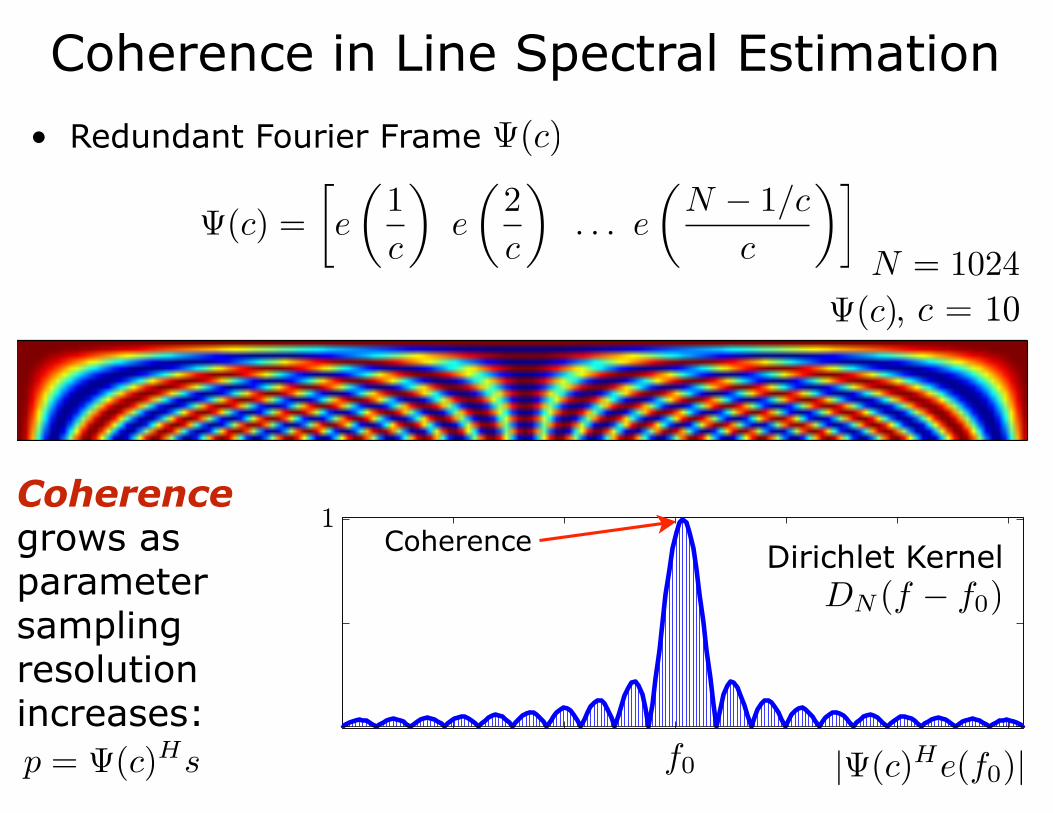
, c = 10
• Redundant Fourier Frame
• Increased resolution allows for more scenes to be formulated as sparse in parametric dictionary
• Neighboring columns become increasingly similar, thereby increasing dictionary coherence:

Resolution in Frequency Domain• Increased resolution allows for more scenes to
be formulated as sparse in parametric dictionary • Neighboring columns become increasingly similar,
thereby increasing dictionary coherence:
• Theorem: If then for each vector there exists at most one K-sparse signal such that
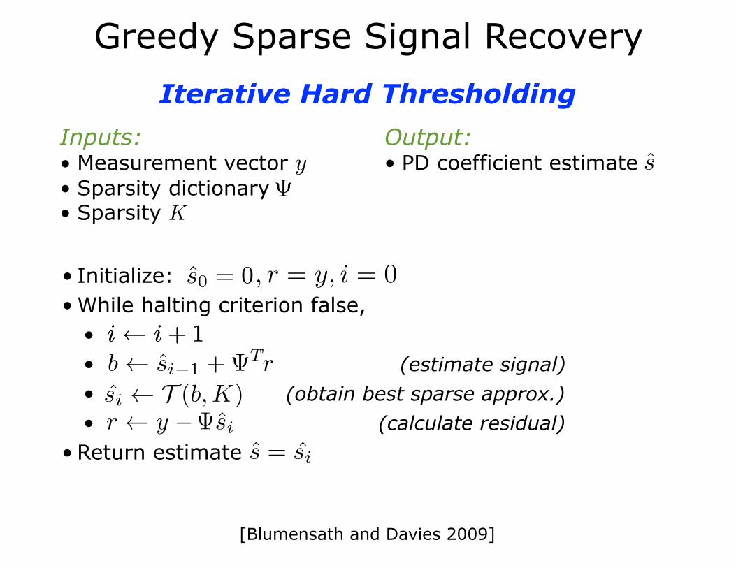
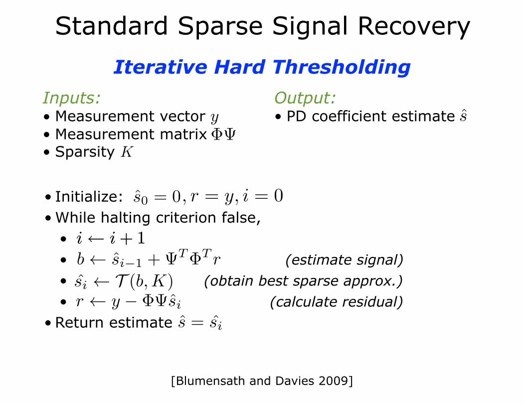
• Initialize: • While halting criterion false,
• • (estimate signal) • (obtain best sparse approx.) • (calculate residual)
• Return estimate
Inputs: • Measurement vector y • Sparsity dictionary • Sparsity K
Greedy Sparse Signal RecoveryIterative Hard Thresholding
Output: • PD coefficient estimate
[Blumensath and Davies 2009]
, c = 10
0 0.02 0.04 0.06 0.08 0.1 0.120
0.5
1
ω
µ(ω
)
0 0.02 0.04 0.06 0.08 0.1 0.120
0.5
1
ω
µ(ω
) > 0
.1
Coherence grows as parameter sampling resolution increases:
Dirichlet Kernel
• Redundant Fourier Frame
Coherence in Line Spectral Estimation
Coherence1

Part 1: Dealing with Coherence
Rich Baraniuk (Rice U.)
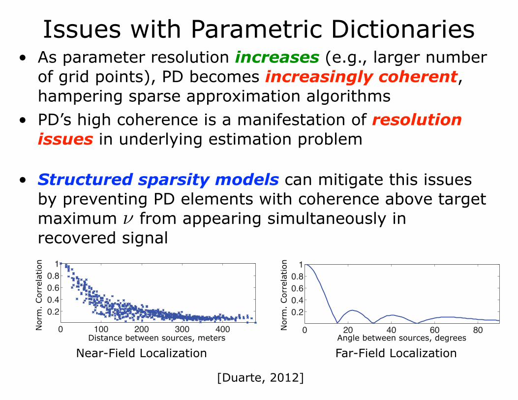
• Structured sparsity models can mitigate this issues by preventing PD elements with coherence above target maximum from appearing simultaneously in recovered signal
0 20 40 60 80
0.2
0.4
0.6
0.8
1
, degrees0 100 200 300 400
0.2
0.4
0.6
0.8
1
, meters
• As parameter resolution increases (e.g., larger number of grid points), PD becomes increasingly coherent, hampering sparse approximation algorithms
• PD’s high coherence is a manifestation of resolution issues in underlying estimation problem
Issues with Parametric Dictionaries
[Duarte, 2012]
Near-Field Localization Far-Field LocalizationDistance between sources, meters
Nor
m.
Cor
rela
tion
Angle between sources, degrees
Nor
m.
Cor
rela
tion
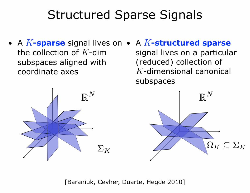
Structured Sparse Signals
• A K-sparse signal lives on the collection of K-dim subspaces aligned with coordinate axes
RN
�K � �K
• A K-structured sparse signal lives on a particular (reduced) collection of K-dimensional canonical subspaces
�K � �K
RN
[Baraniuk, Cevher, Duarte, Hegde 2010]
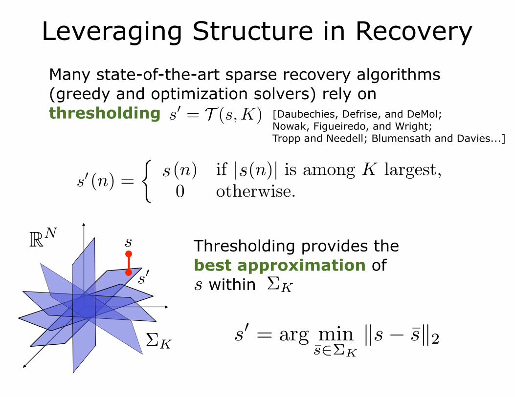
Many state-of-the-art sparse recovery algorithms (greedy and optimization solvers) rely on thresholding
RN
�K � �K
Leveraging Structure in Recovery
[Daubechies, Defrise, and DeMol; Nowak, Figueiredo, and Wright; Tropp and Needell; Blumensath and Davies...]
Thresholding provides the best approximation of s within �K � �K
s s
s
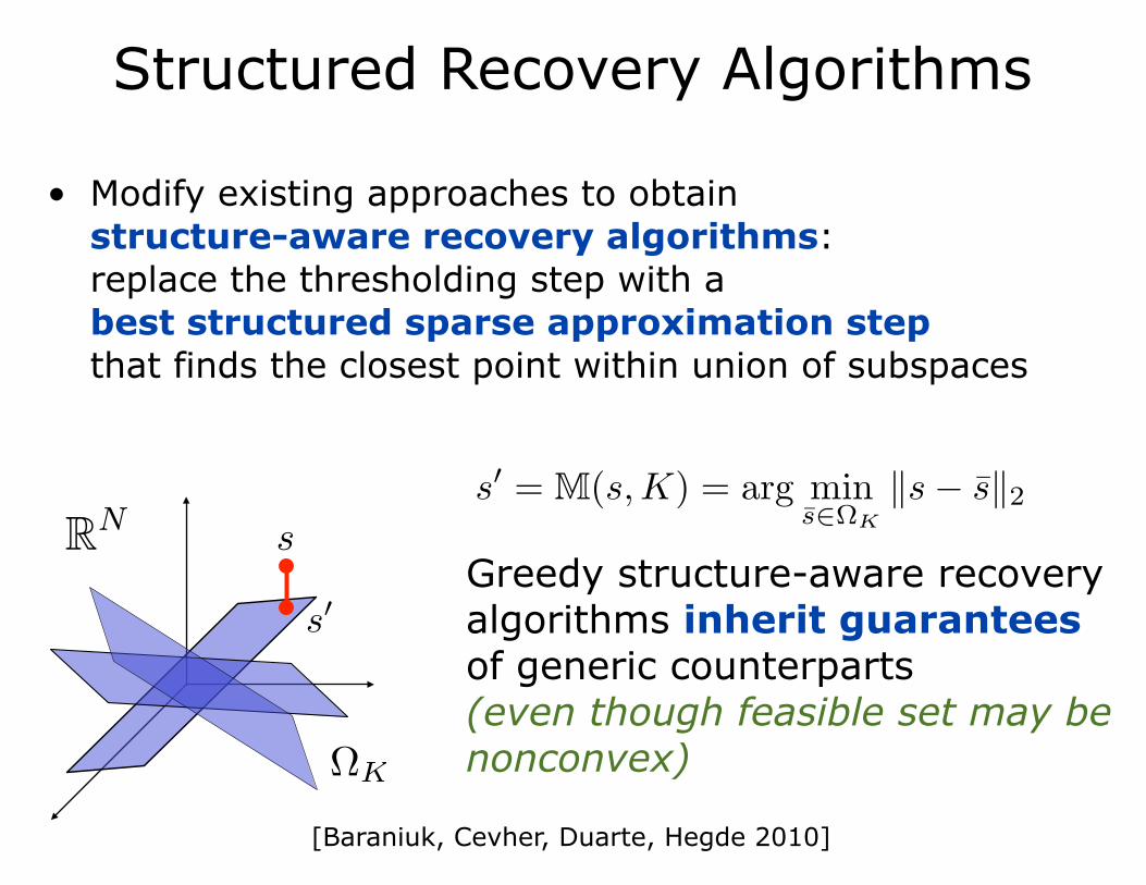
• Modify existing approaches to obtain structure-aware recovery algorithms: replace the thresholding step with a best structured sparse approximation step that finds the closest point within union of subspaces
RN
�K � �K
Greedy structure-aware recovery algorithms inherit guarantees of generic counterparts (even though feasible set may be nonconvex)
Structured Recovery Algorithms
[Baraniuk, Cevher, Duarte, Hegde 2010]
s

• If x is K-structured frequency-sparse, then there exists a K-sparse vector such that and the nonzeros in are spaced apart from each other (band exclusion).
Structured Frequency-Sparse Signals• A K-structured PD-sparse
signal f consists of K PD elements that are mutually incoherent:
RN
if
0 0.02 0.04 0.06 0.08 0.1 0.120
0.5
1
ω
µ(ω
)
0 0.02 0.04 0.06 0.08 0.1 0.120
0.5
1
ω
µ(ω
) > 0
.1
[Duarte and Baraniuk, 2012] [Fannjiang and Liao, 2012]

• Initialize: • While halting criterion false,
• • (estimate signal) • (obtain best sparse approx.) • (calculate residual)
• Return estimate
Inputs: • Measurement vector y • Measurement matrix • Sparsity K
Greedy Sparse Signal RecoveryIterative Hard Thresholding
Output: • PD coefficient estimate
[Blumensath and Davies 2009]

• Initialize: • While halting criterion false,
• • (estimate signal) • (obtain band-excluding sparse approx.) • (calculate residual)
• Return estimate
Output: • PD coefficient estimate
Structured Sparse Signal RecoveryBand-Excluding IHT
Inputs: • Measurement vector y • Measurement matrix • Structured sparse approx.
algorithm
[Duarte and Baraniuk, 2012] [Fannjiang and Liao, 2012]
Can be applied to a variety of greedy algorithms (CoSaMP, OMP, Subspace Pursuit, etc.)

100 200 300 400 50010−2
10−1
100
101
102
Number of Measurements, M
Med
ian
Freq
uenc
y Es
timat
ion
Erro
r, H
z
Standard Sparsity, DFT BasisStandard Sparsity, DFT FrameStructured Sparsity, DFT Frame
Compressive Line Spectral Estimation: Performance Evaluation
N = 1024 K = 20 c = 5
Df = 0.1 Hz for DFT frame
Recovery via IHT Algorithm (or variants)
Sufficient separation between adjacent
frequencies
Part 2: From Discrete to Continuous Models
Karsten Fyhn (Aalborg U.)
Hamid Dadkhahi
S.H. Jensen(Aalborg U.)
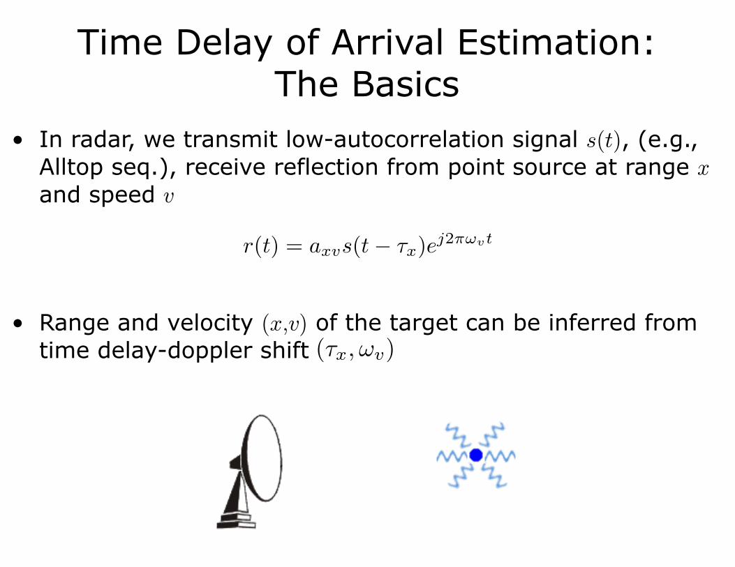
• In radar, we transmit low-autocorrelation signal s(t), (e.g., Alltop seq.), receive reflection from point source at range x and speed v
• Range and velocity (x,v) of the target can be inferred from time delay-doppler shift
Time Delay of Arrival Estimation: The Basics
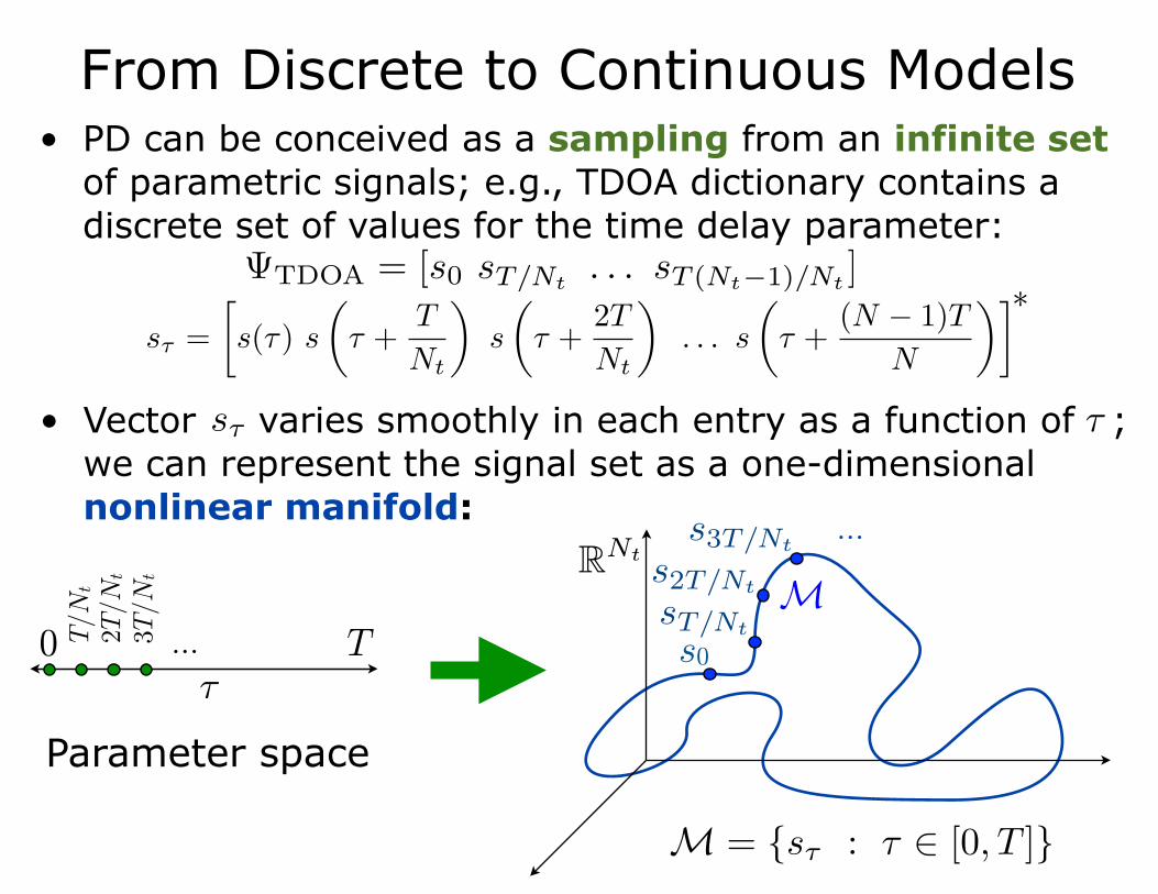
• PD can be conceived as a sampling from an infinite set of parametric signals; e.g., TDOA dictionary contains a discrete set of values for the time delay parameter:
From Discrete to Continuous Models
0 T
Parameter space
• Vector varies smoothly in each entry as a function of ; we can represent the signal set as a one-dimensional nonlinear manifold:
*
T/N
t
2T/N
t
3T/N
t
... s0
...
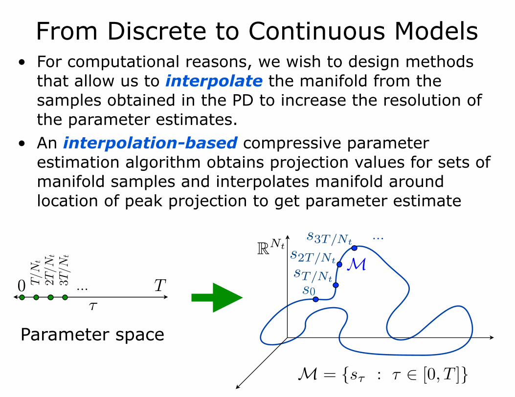
From Discrete to Continuous Models• For computational reasons, we wish to design methods
that allow us to interpolate the manifold from the samples obtained in the PD to increase the resolution of the parameter estimates.
• An interpolation-based compressive parameter estimation algorithm obtains projection values for sets of manifold samples and interpolates manifold around location of peak projection to get parameter estimate
...
0
Parameter space
T s0
T/N
t
2T/N
t
3T/N
t
...
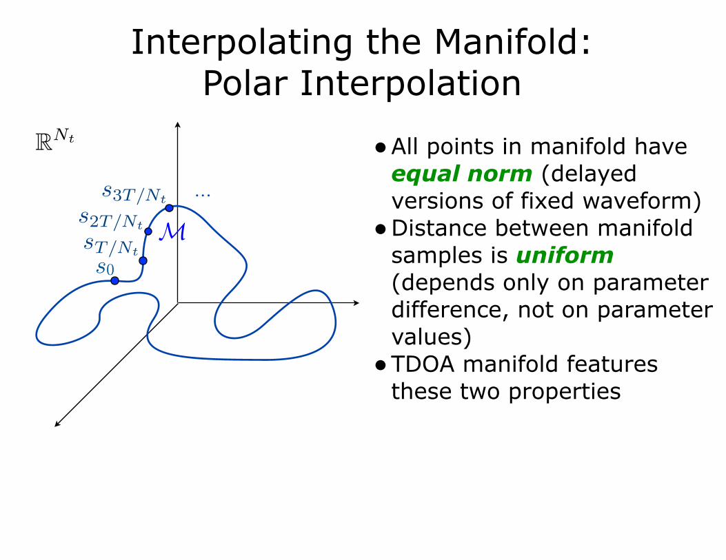
•All points in manifold have equal norm (delayed versions of fixed waveform)
•Distance between manifold samples is uniform (depends only on parameter difference, not on parameter values)
•TDOA manifold features these two properties
...
Interpolating the Manifold: Polar Interpolation
s0
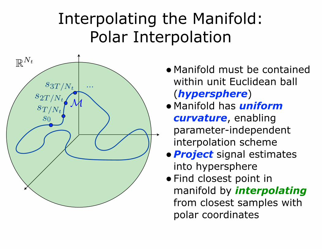
•Manifold must be contained within unit Euclidean ball (hypersphere)
•Manifold has uniform curvature, enabling parameter-independent interpolation scheme
•Project signal estimates into hypersphere
•Find closest point in manifold by interpolating from closest samples with polar coordinates
...
Interpolating the Manifold: Polar Interpolation
s0
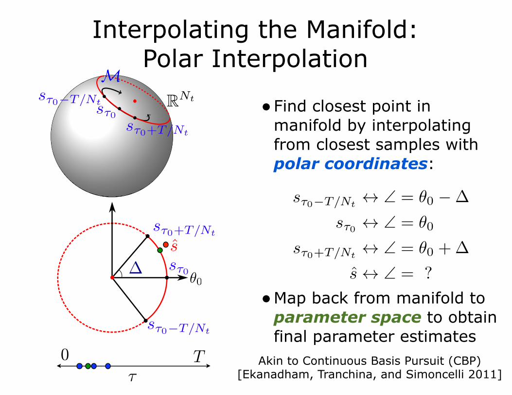
•Find closest point in manifold by interpolating from closest samples with polar coordinates:
•Map back from manifold to parameter space to obtain final parameter estimates
Interpolating the Manifold: Polar Interpolation
Akin to Continuous Basis Pursuit (CBP) [Ekanadham, Tranchina, and Simoncelli 2011]
0 T
• Initialize: • While halting criterion false,
• • (estimate signal) • (obtain best sparse approx.) • (calculate residual)
• Return estimate
Inputs: • Measurement vector y • Measurement matrix • Sparsity K
Standard Sparse Signal RecoveryIterative Hard Thresholding
Output: • PD coefficient estimate
[Blumensath and Davies 2009]
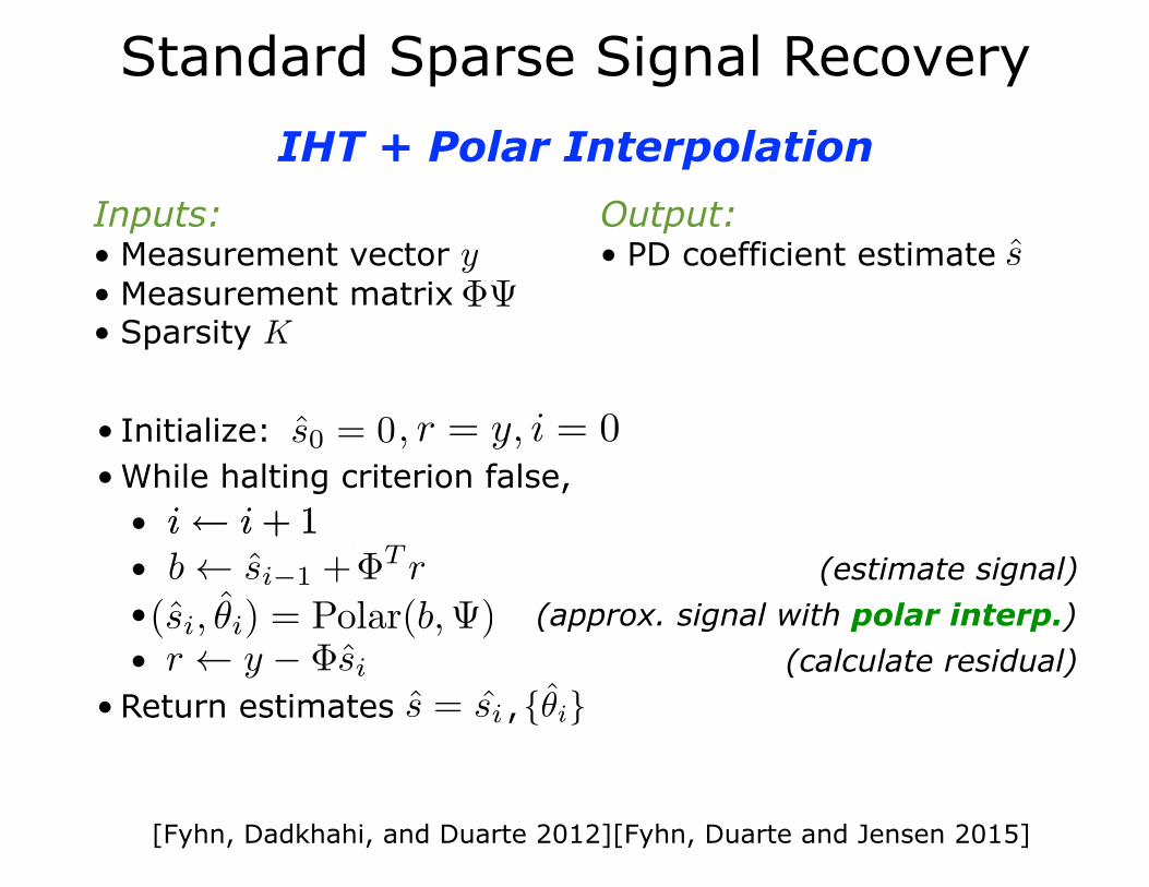
• Initialize: • While halting criterion false,
• • (estimate signal) • (approx. signal with polar interp.) • (calculate residual)
• Return estimates ,
Inputs: • Measurement vector y • Measurement matrix • Sparsity K
Standard Sparse Signal Recovery
Output: • PD coefficient estimate
[Fyhn, Dadkhahi, and Duarte 2012][Fyhn, Duarte and Jensen 2015]
IHT + Polar Interpolation

0.2 0.4 0.6 0.8 110−10
10−8
10−6
10−4
10−2
CS Subsampling Ratio, M/N
Delay
Esti
matio
n MSE
, s2
BOMPBOMP+PolyCS+TDE−MUSICBOMP+CBPBOMP+Polarμ
Compressive Time Delay Estimation: Performance Evaluation
Nt = 500, K = 3, c = 1, .
BOMP [Fannjiang and Liao 2012]
Waveform: chirp of length 1
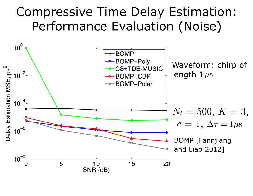
Compressive Time Delay Estimation: Performance Evaluation (Noise)
Nt = 500, K = 3, c = 1, .
BOMP [Fannjiang and Liao 2012]
Waveform: chirp of length 1
0 5 10 15 2010−8
10−6
10−4
10−2
100
SNR (dB)
Dela
y Es
timat
ion
MSE
, µs2
BOMPBOMP+PolyCS+TED−MUSICBOMP+CBPBOMP+Polar
CS+TDE-MUSIC
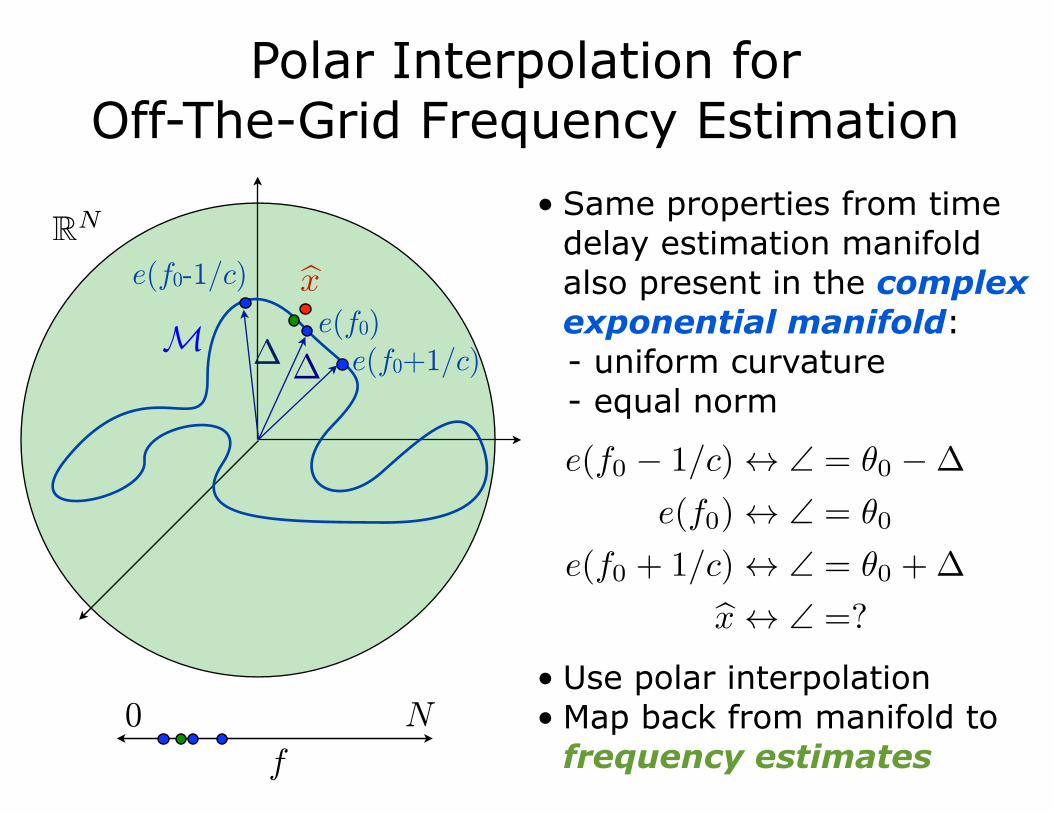
• Same properties from time delay estimation manifold also present in the complex exponential manifold: - uniform curvature - equal norm
• Use polar interpolation • Map back from manifold to
frequency estimates
Polar Interpolation for Off-The-Grid Frequency Estimation
e(f0-1/c)
e(f0+1/c)e(f0)
f
0 N
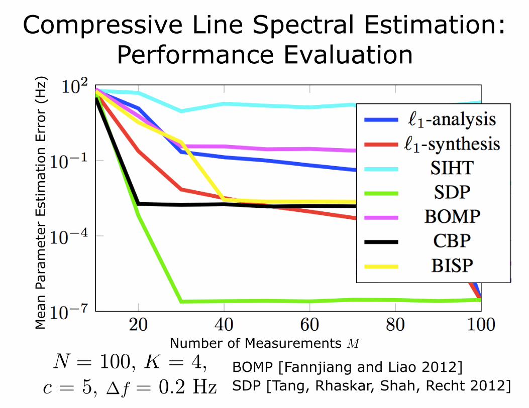
Compressive Line Spectral Estimation: Performance Evaluation
N = 100, K = 4, c = 5, = 0.2 Hz
BOMP [Fannjiang and Liao 2012] SDP [Tang, Rhaskar, Shah, Recht 2012]
Mea
n Pa
ram
eter
Est
imat
ion
Erro
r (H
z)
Number of Measurements M
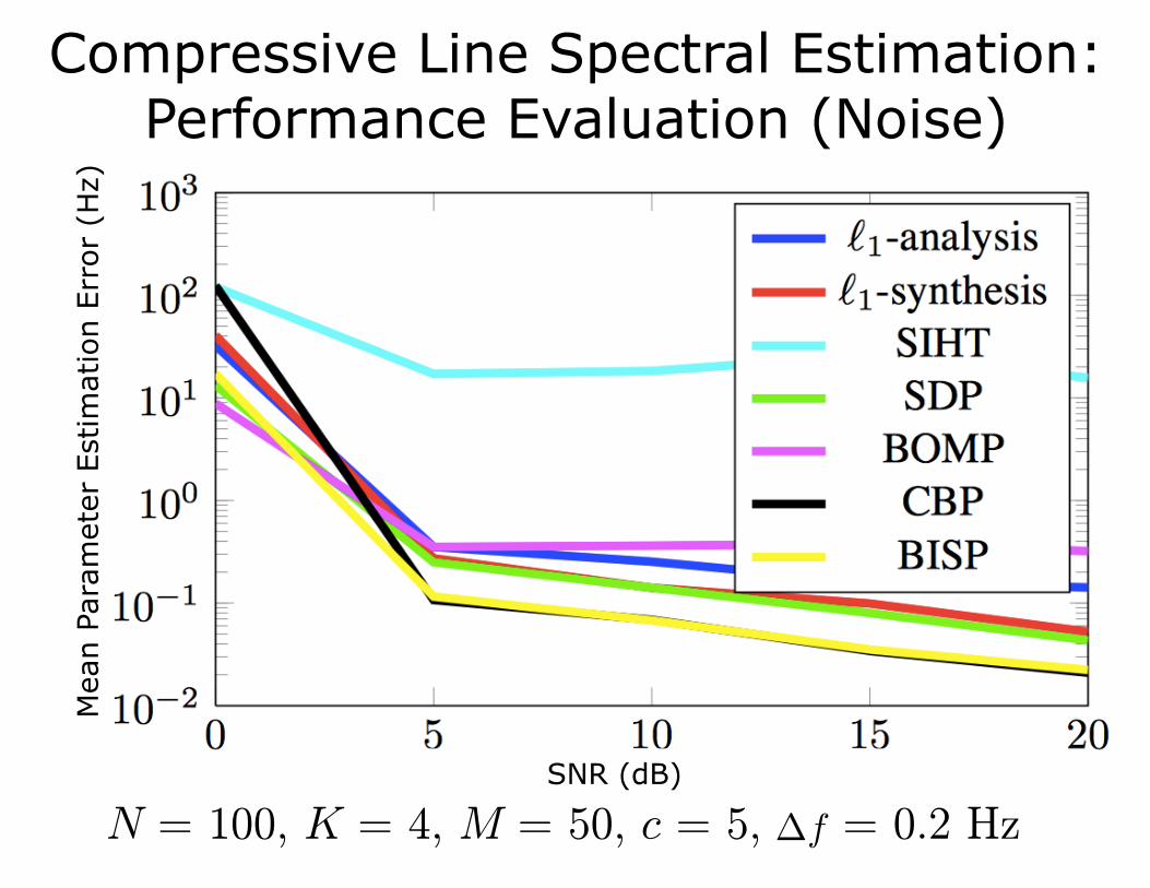
Compressive Line Spectral Estimation: Performance Evaluation (Noise)
N = 100, K = 4, M = 50, c = 5, = 0.2 HzSNR (dB)
Mea
n Pa
ram
eter
Est
imat
ion
Erro
r (H
z)
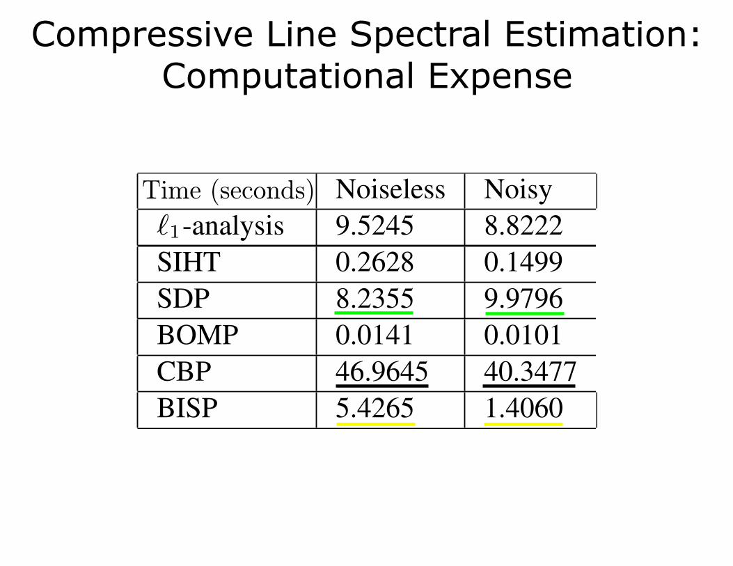
Compressive Line Spectral Estimation: Computational Expense
Algorithm 1 BISPINPUTS: Compressed signal y, sparsity K, measurementmatrix A and spacing between dictionary elements �.OUTPUTS: Reconstructed signal ˜
f and frequency esti-mates ˜!.INITIALIZE: � = AD, i = 1, S
0= ;
while i K doS
0= S
0 [ argmaxi |hy,Aii|, i 62 B0(S0), i = i+ 1
end whiley
0r = y ��S0
�
†S0y, n = 1
LOOP:repeat
i = 1, S
n= S
n�1
while i K doS
n= S
n[argmaxi |hy,Aii|, i 62 B0(Sn), i = i+1
end whilea = (�Sn
)
†y
S
n= supp(thresh(a,K))
⌦ = [{�(s� 1),�s,�(s+ 1)|s 2 S
n}From T(y,A,⌦) obtain ˜
f and ˜! using (9) and (6)y
nr = y �A
˜
f , n = n+ 1
until ||ynr ||2 < ✏ · ||yn�1
r ||2 _ n K
vector or a reconstructed signal (`1-synthesis, `1-analysis,SIHT, and SDP), we apply the MUSIC algorithm [15] on thereconstructed signal to estimate its frequencies. In the BISPand BOMP algorithms, we exclude atoms with coherence⌘ > 0.25 using (4).
For the first experiment, we explore a range of subsam-pling ratios with noiseless measurements to verify the levelof compression that allows for successful estimation. We set✏ = 10
�10 for the relevant algorithms. The result of the nu-merical experiment is shown in Figure 1. In the noiselesscase, SDP obtains the best result. The polar interpolation al-gorithms (CBP and BISP) both converge to a given estimationprecision, which corresponds to the level of approximationerror. When the number of measurements M is sufficientlysmall, CBP outperforms `1-synthesis. The performance ofBOMP and SIHT is worst among the algorithms tested. Sur-prisingly, while the DFT coefficients x found by `1-synthesisare not sparse and do not match the original frequencies, thesignal f is still reconstructed accurately, and so the MUSICalgorithm recovers the frequencies adequately.
For the second experiment, we include measurementnoise in the signal model. We fix = 0.5 and vary the signal-to-noise ratio (SNR) from 0 to 20 dB. In the noisy case, thepolar interpolation algorithms perform best. This is becausetheir interpolation step relies less on the sparsity of the signaland more on the known signal model and the fitting to a circleon the manifold. Additionally, the presence of noise rendersthe measurements non-sparse in the dictionaries used by thenon-interpolating algorithms, hindering their performance.
The computation time of the algorithms is also of impor-
20 40 60 80 100
10
�7
10
�4
10
�1
10
2
Number of measurements (M)
Ave
rage
cost
infr
eque
ncy
estim
atio
n
Fig. 1. Frequency estimation performance in noise-less case.
0 5 10 15 20
10
�2
10
�1
10
0
10
1
10
2
10
3
SNR [dB]A
vera
geco
stin
freq
uenc
yes
timat
ion
`1-analysis`1-synthesis
SIHTSDP
BOMPCBPBISP
Fig. 2. Frequency estimation performance in noisy case.
Noiseless Noisy`1-analysis 9.5245 8.8222`1-synthesis 2.9082 2.7340SIHT 0.2628 0.1499SDP 8.2355 9.9796BOMP 0.0141 0.0101CBP 46.9645 40.3477BISP 5.4265 1.4060
Table 1. Average computation times in seconds.
tance, and we have listed the average computation times inTable 1. We observed that most algorithms exhibit compu-tation time roughly independent of M , with the exception of`1-synthesis and CBP. The table shows that the excellent per-formance of SDP in Figure 1 is tempered by its high computa-tional complexity, as well as its lack of flexibility on the mea-surement scheme. Moreover, the relaxation in BISP that ac-counts for the presence of noise reduces its computation time,increasing its performance advantage over SDP and CBP.
Time (seconds)
Part 3: Meaningful Performance Metrics
Dian Mo
0.2 0.4 0.6 0.8 110−1
100
101
κ
Aver
age
Para
met
er E
stim
atio
n [ µ
s]
T =1 µsT =2 µsT =3 µsT =4 µsT =5 µs
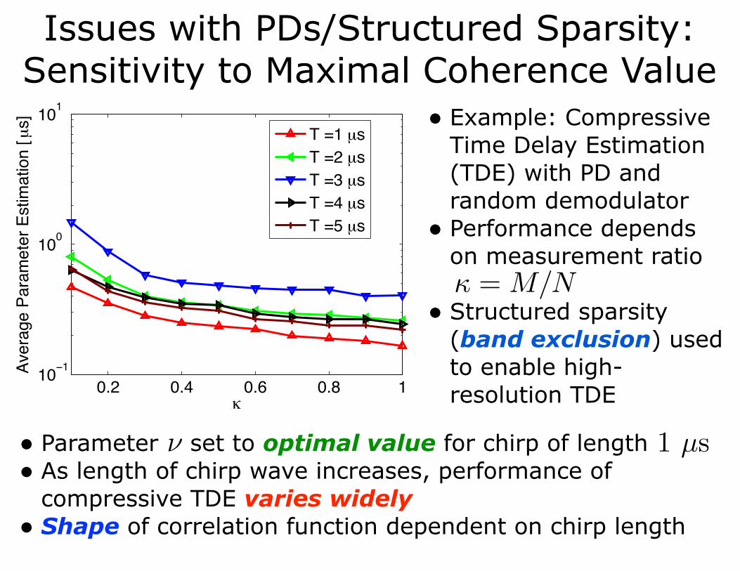
Issues with PDs/Structured Sparsity: Sensitivity to Maximal Coherence Value
• Example: Compressive Time Delay Estimation (TDE) with PD and random demodulator
• Performance depends on measurement ratio
• Structured sparsity (band exclusion) used to enable high-resolution TDE
• Parameter set to optimal value for chirp of length • As length of chirp wave increases, performance of
compressive TDE varies widely • Shape of correlation function dependent on chirp length
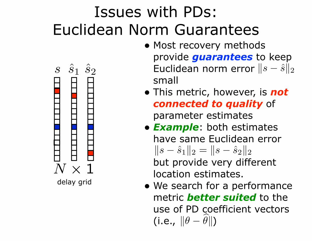
Issues with PDs: Euclidean Norm Guarantees
• Most recovery methods provide guarantees to keep Euclidean norm error small
• This metric, however, is not connected to quality of parameter estimates
• Example: both estimates have same Euclidean errorbut provide very different location estimates.
• We search for a performance metric better suited to the use of PD coefficient vectors (i.e., )
delay grid
s
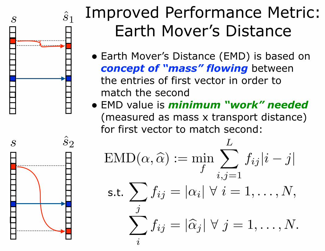
Improved Performance Metric: Earth Mover’s Distance
• Earth Mover’s Distance (EMD) is based on concept of “mass” flowing between the entries of first vector in order to match the second
• EMD value is minimum “work” needed (measured as mass x transport distance) for first vector to match second:
s.t.
s
s
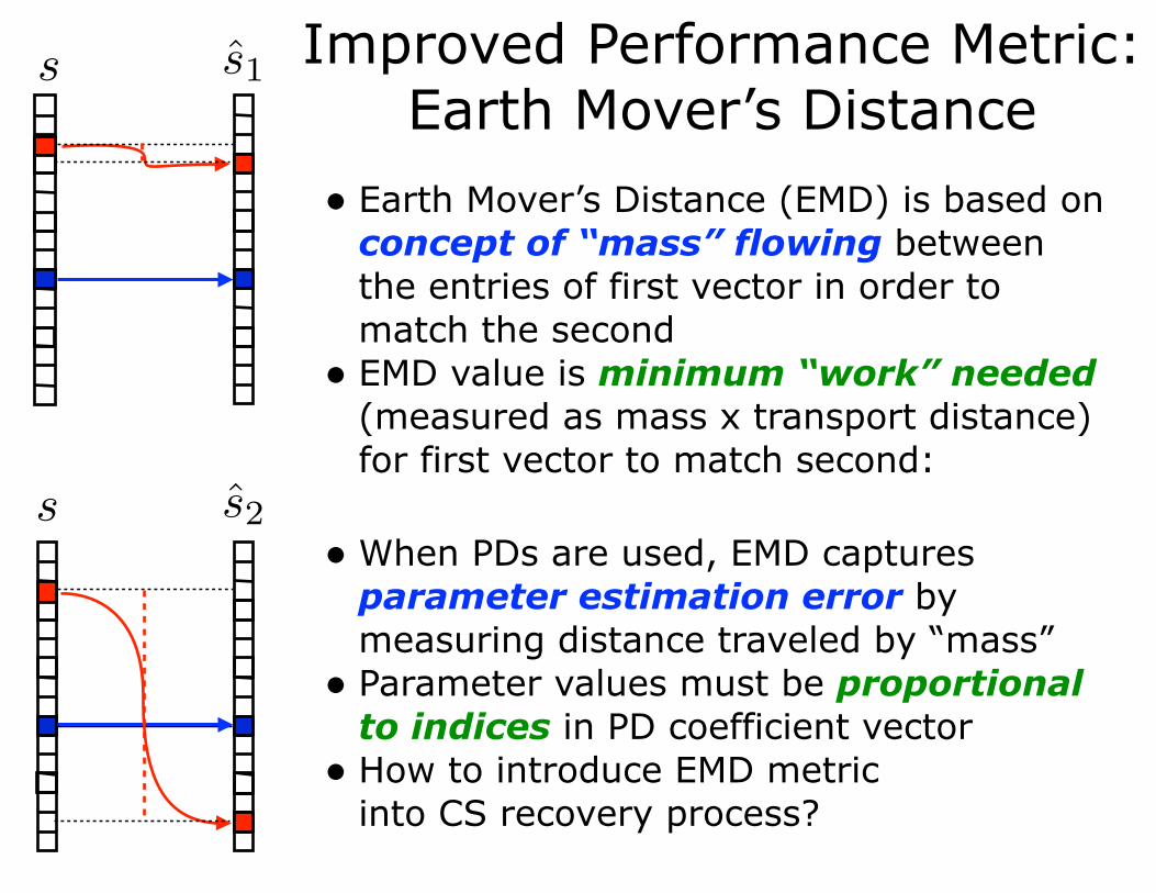
Improved Performance Metric: Earth Mover’s Distance
• When PDs are used, EMD captures parameter estimation error by measuring distance traveled by “mass”
• Parameter values must be proportional to indices in PD coefficient vector
• How to introduce EMD metric into CS recovery process?
• Earth Mover’s Distance (EMD) is based on concept of “mass” flowing between the entries of first vector in order to match the second
• EMD value is minimum “work” needed (measured as mass x transport distance) for first vector to match second:
s
s
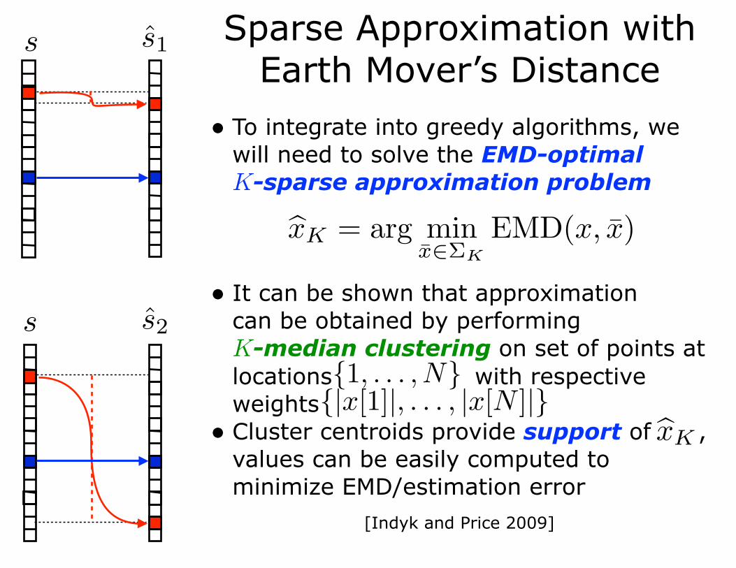
• To integrate into greedy algorithms, we will need to solve the EMD-optimal K-sparse approximation problem
• It can be shown that approximation can be obtained by performing K-median clustering on set of points at locations with respective weights
• Cluster centroids provide support of , values can be easily computed to minimize EMD/estimation error
Sparse Approximation with Earth Mover’s Distance
[Indyk and Price 2009]
s
s
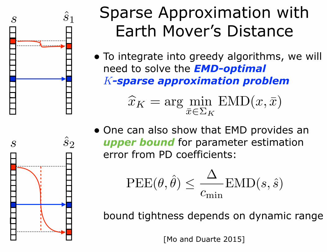
• To integrate into greedy algorithms, we will need to solve the EMD-optimal K-sparse approximation problem
• One can also show that EMD provides an upper bound for parameter estimation error from PD coefficients:bound tightness depends on dynamic range
Sparse Approximation with Earth Mover’s Distance
[Mo and Duarte 2015]
s
s
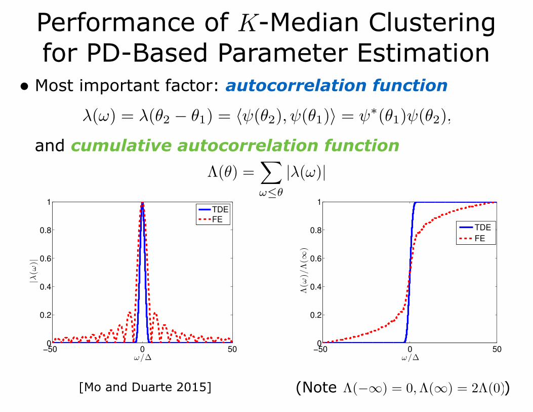
• Most important factor: autocorrelation function and cumulative autocorrelation function
Performance of K-Median Clustering for PD-Based Parameter Estimation
[Mo and Duarte 2015]
−50 0 500
0.2
0.4
0.6
0.8
1
ω/∆
Λ(ω
)/Λ(∞
)
TDE
FE
−50 0 500
0.2
0.4
0.6
0.8
1
ω/∆
|λ(ω
)|
TDE
FE
(Note )
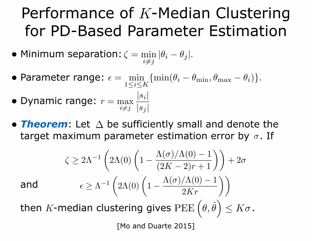
• Minimum separation:
• Parameter range:
• Dynamic range:
• Theorem: Let be sufficiently small and denote the target maximum parameter estimation error by . If
and then K-median clustering gives .
Performance of K-Median Clustering for PD-Based Parameter Estimation
[Mo and Duarte 2015]
ζ [µs]0.07 0.08 0.09 0.1
σ[µs]
0.00
0.20
0.40
0.60
0.80x 10
-2
Performance of K-Median Clustering for PD-Based Parameter Estimation
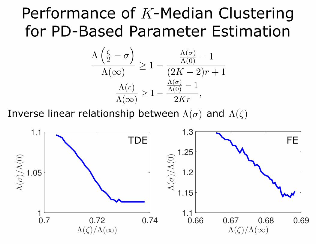
Inverse linear relationship between and
Λ(ζ)/Λ(∞)0.7 0.72 0.74
Λ(σ)/Λ(0)
1
1.05
1.1
Λ(ζ)/Λ(∞)0.66 0.67 0.68 0.69
Λ(σ)/Λ(0)
1.1
1.15
1.2
1.25
1.3
TDE FE
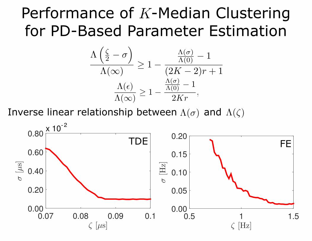
ζ [µs]0.07 0.08 0.09 0.1
σ[µs]
0.00
0.20
0.40
0.60
0.80x 10
-2
ζ [Hz]0.5 1 1.5
σ[H
z]
0.00
0.05
0.10
0.15
0.20x 10
0
Performance of K-Median Clustering for PD-Based Parameter Estimation
TDE FE
2
Inverse linear relationship between and

• Initialize: • While halting criterion false,
• • (estimate signal) • (obtain band-excluding sparse approx.) • (calculate residual)
• Return estimate
Output: • PD coefficient estimate
Structured Sparse Signal RecoveryBand-Excluding IHT
Inputs: • Measurement vector y • Measurement matrix • Structured sparse approx.
algorithm
[Duarte and Baraniuk, 2012] [Fannjiang and Liao, 2012]
Can be applied to a variety of greedy algorithms (CoSaMP, OMP, Subspace Pursuit, etc.)

• (calculate residual) • Return estimate
• Initialize: • While halting criterion false,
• • (estimate signal) • (best sparse approx. in EMD)
Output: • PD coefficient estimate
Inputs: • Measurement vector y • Measurement matrix • Sparsity K
EMD + Sparse Signal Recovery
Can be applied to a variety of greedy algorithms (CoSaMP, OMP, Subspace Pursuit, etc.)
Clustered IHT
[Mo and Duarte, 2014]
Numerical Results
0.2 0.4 0.6 0.8 110−1
100
101
κ
Aver
age
Para
met
er E
stim
atio
n [ µ
s]
T =1 µsT =2 µsT =3 µsT =4 µsT =5 µs
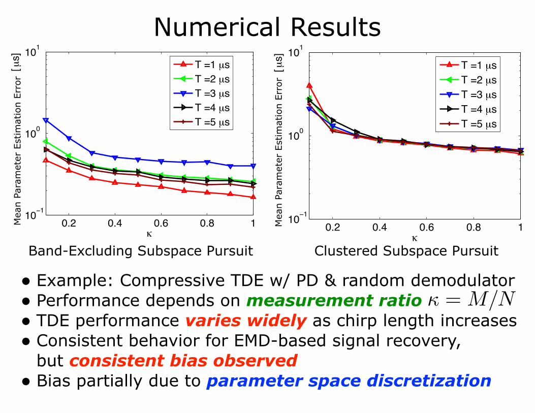
• Example: Compressive TDE w/ PD & random demodulator • Performance depends on measurement ratio • TDE performance varies widely as chirp length increases • Consistent behavior for EMD-based signal recovery,
but consistent bias observed • Bias partially due to parameter space discretization
0.2 0.4 0.6 0.8 110−1
100
101
κ
Aver
age
Para
met
er E
stim
atio
n [ µ
s]
T =1 µsT =2 µsT =3 µsT =4 µsT =5 µs
Band-Excluding Subspace Pursuit Clustered Subspace Pursuit
Mea
n Pa
ram
eter
Est
imat
ion
Erro
r
Mea
n Pa
ram
eter
Est
imat
ion
Erro
r
0.2 0.4 0.6 0.8 110−20
10−15
10−10
10−5
100
κ
Aver
age
Para
met
er E
stim
atio
n [ µ
s]
T =1 µsT =2 µsT =3 µsT =4 µsT =5 µs
Numerical Results
0.2 0.4 0.6 0.8 110−20
10−15
10−10
10−5
100
κ
Aver
age
Para
met
er E
stim
atio
n [ µ
s]
T =1 µsT =2 µsT =3 µsT =4 µsT =5 µs
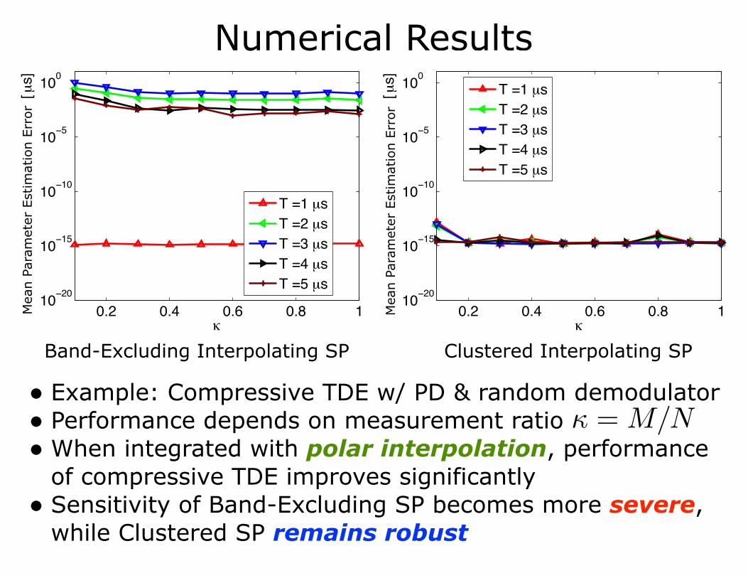
• Example: Compressive TDE w/ PD & random demodulator • Performance depends on measurement ratio • When integrated with polar interpolation, performance
of compressive TDE improves significantly • Sensitivity of Band-Excluding SP becomes more severe,
while Clustered SP remains robust
Band-Excluding Interpolating SP Clustered Interpolating SP
Mea
n Pa
ram
eter
Est
imat
ion
Erro
r
Mea
n Pa
ram
eter
Est
imat
ion
Erro
r
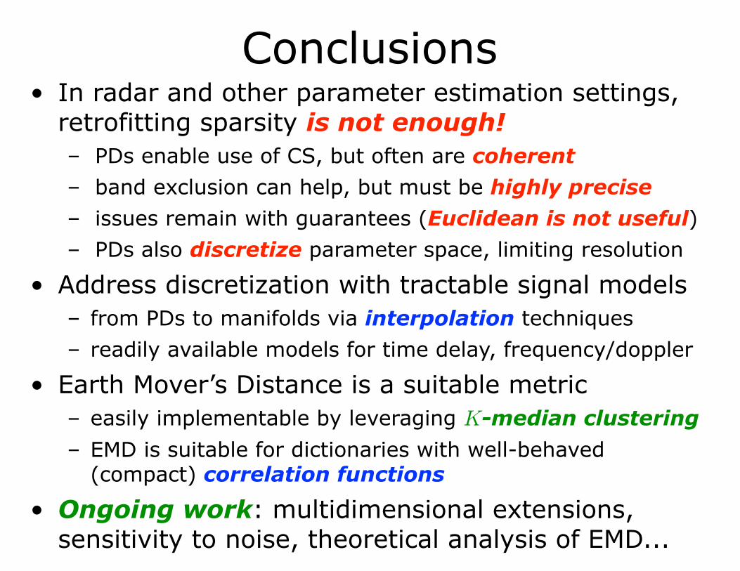
Conclusions• In radar and other parameter estimation settings,
retrofitting sparsity is not enough! – PDs enable use of CS, but often are coherent – band exclusion can help, but must be highly precise – issues remain with guarantees (Euclidean is not useful) – PDs also discretize parameter space, limiting resolution
• Address discretization with tractable signal models – from PDs to manifolds via interpolation techniques – readily available models for time delay, frequency/doppler
• Earth Mover’s Distance is a suitable metric – easily implementable by leveraging K-median clustering – EMD is suitable for dictionaries with well-behaved
(compact) correlation functions
• Ongoing work: multidimensional extensions, sensitivity to noise, theoretical analysis of EMD...
References
http://www.ecs.umass.edu/~mduarte [email protected]
• M. F. Duarte and R. G. Baraniuk, “Spectral Compressive Sensing,” Applied and Computational Harmonic Analysis, Vol. 35, No. 1, pp. 111-129, 2013.
• M. F. Duarte, “Localization and Bearing Estimation via Structured Sparsity Models,” IEEE Statistical Signal Processing Workshop (SSP), Aug. 2012, Ann Arbor, MI, pp. 333-336.
• K. Fyhn, H. Dadkhahi, and M. F. Duarte, “Spectral Compressive Sensing with Polar Interpolation,” IEEE International Conference on Acoustics, Speech, and Signal Processing (ICASSP), May 2013, Vancouver, Canada, pp. 6225-6229.
• K. Fyhn, M. F. Duarte, and S. H. Jensen, “Compressive Parameter Estimation for Sparse Translation-Invariant Signals Using Polar Interpolation,” IEEE Transactions on Signal Processing, Vol. 63, No. 4, pp. 870-881, 2015.
• D. Mo and M. F. Duarte, “Compressive Parameter Estimation with Earth Mover’s Distance via K-Median Clustering,” Wavelets and Sparsity XV, SPIE Optics and Electronics, Aug. 2013, San Diego, CA.
• D. Mo and M. F. Duarte, “Compressive Parameter Estimation via K-Median Clustering”, arXiv:1412.6724, December 2014.


![[Engelberg] Compressive Sensing](https://img.pdfslide.us/doc/110x75/55cf9985550346d0339dc8ee/engelberg-compressive-sensing.jpg)