Parameter Estimation for Stochastic Models of

Interacting Agents:

An Approximate ML Approach

Thomas LuxDepartment of Economics

University of Kiel ∗

November 29, 2006

Abstract

Simple models of interacting agents can be formulated as jump Markovprocesses via suitably specified transition probabilities. Their aggregatedynamics might then be analyzed by the Master equation for the change ofthe probability distribution over time, or the Fokker-Planck equation thatis obtained by a power series expansion and governs the probability distri-bution for fluctuations around an equilibrium. With such information onthe transient density of the process, maximum likelihood estimation of itsparameters becomes feasible. Even if the Fokker-Planck equation can notbe solved explicitly, one can resort to numerical approximations like theCrank-Nicolson method for approximate ML estimation. We explain thisalgorithm with a simple model of interacting agents and show that theapproximate ML procedure works well and has desirable accuracy even inthe case of bimodal limiting distributions. We illustrate possible applica-tions by estimating the parameters of this model for a popular businessclimate index for the German economy.

- preliminary version -

∗Financial support from the EU STREP ComplexMarkets (contract number 516446) isgratefully acknowledged.

1

1 The basic framework

Many agent-based models with simple rules of agents’ adaption to external in-fluences allow for a representation of their aggregate quantities via Markovianstochastic processes. A comprehensive formalization of the time developmentof the probability distribution over their configuration space can be attemptedvia the Master equation formalism or approximations to it such as the Fokker-Planck equation for the dynamics of the transitional density (cf. the seminalmethodological contributions by Weidlich and Haag, 1983; Aoki, 1996; and Wei-dlich, 2002). In the following we will particularly focus on the fertilization ofthe Fokker-Planck equation for estimation of the parameters of the underlyinghypothetical model. The Fokker-Planck equation associated to a stochastic pro-cess is a parabolic differential equation for the change in time of the transitorydensity of the process. Although the Fokker-Planck equation occupies a veryprominent place in statistical physics (Risken, 1989; Frank, 2005), it seems thatdue to the different research perspectives in this field, it has never been used asa tool for estimation of parameters of physical models.

Nevertheless, the use of the Fokker-Planck equation for parameter estima-tion is straight forward: if on has available discrete observations of a diffusionprocess and if the Fokker-Planck equation of the hypothesized process could besolved explicitly, the time-dependent solution to the transient density at thetimes of observations could be used to estimate the parameters via a standardmaximum likelihood approach. Unfortunately, in models of interacting agents,a closed-form solution to the Fokker-Planck equation is usually not available. Inthis case, however, we could resort to numerical approximations of the Fokker-Planck equations. Numerical integration of partial differential equations via fi-nite difference of finite element methods is also a well developed field (Thomas,1995) and has found important applications both in statistical physics (Park andPetrosian) and financial mathematics (Seydel, 2002, part III). A well-known areaof application is the pricing of American options and exotic options for whichno closed-form solutions of the modified Black-Scholes equation exist. The onlyapplication within an estimation framework can be found in a different branchof computational finance, namely diffusion processes of the term structure ofinterest rates. The first to propose approximate ML estimation on the base ofa numerical integration of transitory densities has been Poulsen (1999) whoseapproach has been compared to alternative methods by Jensen and Poulsen(2002). Hurn et al. (2006) propose refinements using finite elements ratherthan finite differences.

In order to set the stage for the presentation of this methodology, considera parabolic stochastic differential equation:

∂f(x)∂t

=∂

∂x(µ(x, θ)f(x)) +

∂2

∂x2(g(x, θ)f(x)) (1)

2

If (1) refers to a Fokker-Planck equation, the unknown function f(x, t) is thetransitory density of x, and we can write µ(x, θ) = −A(x, θ) , g(x, θ) = 1

2D(x, θ)with A(x, θ) and D(x, θ) the drift and diffusion functions of the process, and θa set of unknown parameters that one wants to estimate.

If no closed-form solution for f(x, t) is available (which will mostly be thecase), one can study the time development of the density via numerical inte-gration of eq.(1). Various methods for discretisation of the stochastic equation(1) can be used. If one uses an evenly spaced discrete grid, one speaks of finitedifference methods, if one uses a flexible grid, one speaks of refined finite elementmethods.

In principle, the first and second derivatives on both sides of eq. (1) couldbe approximated either via forward differences of backward differences (calledexplicit or implicit methods). Higher accuracy of the approximation can beachieved by combining both forward and backward differences by computingcentral differences around intermediate grid points. This approach is known asthe Crank-Nicolson method and will be adopted in what follows.

To concretize the finite difference approximation, consider a ‘space’ grid withdistance h between adjacent knots: xj = x0 + j ·h; j = 0, 1, ..., Nx and similarlyequally spaced points along the time axis between t = 0 and the final time T :ti = i · k with i = 0, ..., Nt and k = T

Nt.

In a forward discretization, (1) would have to be replaced by

f i+1j − f i

j

k=

µj+1fij+1 − µjf

ij

h+

gj+1fij+1 − 2gjf

ij + gj−1f

ij−1

h2(2)

with f ij := f(x0 + j · h, ik) and µj := µ(x0 + j · h, θ), gj := g(x0 + j · h, θ).

Replacing the forward difference on the left-hand side by the backward differ-ence f i

j−f i−1j , we obtain the implicit finite difference approximation. While the

forward and backward approximations are of local accuracy (at the mesh points)O(k)+O(h2), higher accuracy can be obtained by taking the average of both theforward and backward difference approximation. This is known as the Crank-Nicolson method and can be shown to have local accuracy O(k2)+O(h2). Notethat the Crank-Nicolson approach effectively approximates the continuous-timediffusion at intermediate points (i + 1

2 )k and (j + 12 )h rather than those on the

grid itself.

Because of the necessity of restricting the approximation to a finite interval,boundary conditions have to be imposed in order to prevent transitions to in-

3

accessible states. In the Crank-Nicolson approach this requires the assumption

f j

− 12

= f(x0− 12h, jk) = 0 and f j

N+ 12

= f(x0 +(Nx +12)h, jk) = 0 (3)

(cf. Giuliani). While such simple Dirichlet boundary conditions preservethe local second order accuracy, more complex derivative boundary conditionsin certain applications would require a careful analysis of the errors broughtabout by their discretization. It is important to note that the no-flux boundaryconditions guarantee conservation of probability mass within the underlyingx-interval if (1) governs the dynamics of a transient density (i.e. if (1) is aFokker-Planck equation).

The second order accuracy of the Crank-Nicolson scheme can be checked inapplications by trying different step sizes h or k. Denote by v1, v2 and v3 theapproximations of the continuous solution f , using step sizes k and h, h

2 andh4 , respectively. Then by expanding the error of the approximation in a Taylorseries:

v1 = f − hc− kd− h2l − k2m + ... (4)

v2 = f − 0.5hc− kd− 0.25h2l − k2m + ... (5)

v3 = f − 0.25hc− kd− 0.0625h2l − k2m + ... (6)

It follows that the quotient of the differences of these approximations yields:

v2 − v1

v3 − v2' 2

c + 1.5hl

c + 0.75hl(7)

Hence, if the method is first-order accurate, c 6= 0 should be the dominatingcomponent and evaluating (7) at the grid points, we would expect to see valuesclose to 2. On the contrary, prevalence of values around 4 all over the placewould be seen as a confirmation of the theoretical second-order accuracy of theCrank-Nicolson scheme. The same operation can be performed in the time di-rection as well using differences k, k

2 , and k4 . We will see an illustration of this

experimental determination of the order of accuracy in our application below.

On the base of the Crank-Nicolson (or any other finite difference approxi-mation), we can estimate the parameters of a diffusion process with discretelyspaced observations via approximate maximum likelihood.

4

The negative log-likelihood of a sample of observations X0, . . . , XT is

−logf0(X0 | θ)−T−1∑s=0

logf(Xs+1 | Xs, θ) (8)

where f0(X0 | θ) is the density of the initial state (which in practical appli-cations will be skipped because of its negligible influence and the possible lackof a closed-form solution for the stationary density) and f(Xs+1 | Xs, θ) is thevalue of the transitional density at s+1 conditioned on the previous observationat time s,Xs. This continuous density is approximated by our finite differencescheme. Poulsen (1999) shows that the pertinent estimator is consistent, asymp-totically normal and can be asymptotically equivalent to full ML estimates, atleast under the Crank-Nicolson approximation scheme.

2 Finite difference approximation of a canoni-cal’ interaction model

For illustration of the above framework, we use an approach that goes back atleast to Weidlich and Haag (1983) and had been used in a macroeconomic settingby Kraft, Landes and Weise (1986) among others and in behavioral financemodels by Lux (1995, 1997). The model deals with a binary choice problemand stochastic transitions of agents between both alternatives due to exogenousfactors and group pressure. Let the two groups have occupation numbers n+

and n− ,respectively, with the overall population size being 2N (multiplicationby 2 simply serves to avoid the case of an odd number of individuals).The socio-economic configuration at any time can be described via the differencebetween group occupation numbers:

n =12(n+ − n−) (9)

or an equivalent opinion index:

x =n

N=

n+ − n−2N

with x ∈ [−1, 1]. (10)

A simple stochastic process of individual moves between groups can be builtupon Poisson probabilities to jump from the “+” to the “−” group or vice versawithin the next instant. We denote this transition rates by w↑ and w↓ andassume that they are the same for all agents within our group.For the sake of our illustration, we follow the earlier literature assuming anexponential functional form of w↑ and w↓:

w↑ = v exp(U), w↓ = v exp(−U) (11)

5

The forcing function U is assumed to consist of a constant factor (bias) α0

and a second component formalizing group pressure in favor or against homo-geneous decisions, α1x:

U = α0 + α1x. (12)

The parameters of the model are, thus: v which determines the frequency(time scale) of moves between groups, α0 which generates a bias towards thechoice of “+” (“−”) if positive (negative) and α1 which formalizes the degree ofgroup pressure (if it is positive, if negative it would rather imply a tendency ofnon-conformity). Models with this basic ingredients have been thoroughly in-vestigated in the literature. The basic outcome of the model can be summarizedby the following findings:

i) For α1 ≤ 1, the group dynamics defined by (11) and (12) is characterizedby a stationary distribution with a unique maximum. If α0 = 0, thismaximum is located at x∗ = 0. It shifts to the right (left) for α0 > 0,(< 0).

ii) For α1 > 1 and α0 not too large, the stationary distribution has twomaxima. If α0 = 0, the distribution is symmetric around 0. It becomesasymmetric if α0 6= 0 with right-hand (left-hand) skewness and more con-centration of probability mass in the right (left) maximum if α0 > 0, (< 0)holds.

iii) If |α0| becomes very large, the smaller mode vanishes and the station-ary distribution becomes uni-modal again. This happens if |α0| increasesbeyond the bifurcation value α0 given by:

cosh2(α0 −√

α1(α1 − 1)) = α1 (13)

In most applications, the first step towards an analysis of the above groupdynamics consists in the derivation of a quasi-deterministic law of motion forthe first moment of x:

d

dtx = v(1− x)eα0+α1x − v(1 + x)e−α0−α1x (14)

(14) is exact in the limit of an infinite population size and provides a first-order approximation of the dynamics of x for finite populations.

One easily recovers that the features of the unconditional distribution ((i) to(iii)) are reflected in the existence and stability of steady states of (14).

A more comprehensive description of the dynamics can be obtained via theFokker-Planck equation. Its drift component can be shown to be:

6

A(x) =n−2N

w↑(x)− n+

2Nw↓(x) = v(1− x)eα0+α1x − v(1 + x)e−α0−α1x (15)

which, of course, coincides with the right-hand side of (14), while the diffu-sion term is:

D(x) =1N

(n−2N

w↑(x)+n+

2Nw↓(x)) =

1N

(v(1−x)eα0+α1x +v(1+x)e−α0−α1x)

(16)

This is certainly a case in which the conditional density can not be solved forexplicitly due to the high degree of non-linearity of both the drift and diffusioncomponents. For numerical integration, we can, however, resort to the Crank-Nicolson scheme as introduced above. Fig. 1 shows an example with a stronglypeaked initial distribution which evolves into a bi-modal distribution over time.Underlying parameters are: v = 3, α0 = 0, α1 = 1.2, N = 50 for the parametersof the agent-based model, h = 0.0025 and k = 0.01 for the discretization inspace and time, T = 2 for the time horizon of the numerical integration and aspace grid extending from −1 to 1 in accordance with the support of the variablex has been used. The initial condition, x0 = 0, has been approximated by aNormal distribution density ΦN (x0 + A(x)k, D(x)k) evaluated at grid points−1 + jh; j = 0, 1, . . . , Nx, in the x direction for the first time increment k.This avoids the problems of a Dirac δ-function as initial condition and canbe interpreted as a first-order Euler approximation using the known drift anddiffusion functions for the initialization of the approximation.

We proceed by checking the theoretical second-order accuracy of our ap-proximation. We perform the order determination separately in each directionfor the approximation exhibited in Fig. 1. Table 1 exhibits results for selectedgrid points with (7) applied to both the h and k distances. As can be seen, theexpected dominance of values close to 4 is nicely confirmed and we can convinceourselves that the algorithm has no problem in tracking the transition fromuni-modality to bi-modality with the required degree of accuracy.

x|t 0.25 0.5 0.75 1 1.25 1.5 1.75 2-0.75 4.0 4.0 3.9 4.0 4.0 4.0 4.0 3.9-0.5 4.0 4.0 4.0 4.0 4.0 4.0 4.0 4.0-0.25 4.0 4.0 4.0 4.0 4.0 4.0 4.0 4.0

0 4.0 4.0 4.0 4.0 4.0 4.0 4.0 4.00.25 4.0 4.0 4.0 4.0 4.0 4.0 4.0 4.00.5 4.0 4.0 4.0 4.0 4.0 4.0 4.0 4.00.75 4.0 4.0 3.9 4.0 4.0 4.0 4.0 3.9

h-ratio

7

x|t 0.25 0.5 0.75 1 1.25 1.5 1.75 2-0.75 4.0 3.9 4.0 4.0 4.0 4.0 4.0 4.0-0.5 3.9 4.0 4.0 4.0 4.0 4.0 4.0 4.0-0.25 3.9 4.0 4.0 4.0 4.0 4.0 4.0 4.0

0 6.1 4.0 4.0 4.0 4.0 4.0 4.0 4.00.25 3.9 4.0 4.0 4.0 4.0 4.0 4.0 4.00.5 3.9 4.0 4.0 4.0 4.0 4.0 4.0 4.00.75 4.0 4.0 4.0 4.0 4.0 4.0 4.0 4.0

k-ratio

Table 1: Order determination for the Crank-Nicolson method applied to theinteracting agent model. All parameter values and settings like in Fig. 1

x|t 0.25 0.5 0.75 1 1.25 1.5 1.75 2-0.75 6.1 4.2 4.0 4.0 4.0 4.0 4.1 4.1-0.5 5.0 4.1 4.0 4.0 4.1 4.1 4.2 4.2-0.25 4.4 4.0 4.0 4.1 4.2 4.5 4.9 4.8

0 4.1 4.0 4.1 7.2 3.4 3.5 3.3 2.10.25 4.0 4.2 3.7 3.7 3.6 3.2 5.9 4.40.5 4.1 3.6 5.7 4.2 4.1 4.1 4.0 4.00.75 4.4 4.0 4.0 4.0 4.0 4.0 4.0 4.0

h-ratio

x|t 0.25 0.5 0.75 1 1.25 1.5 1.75 2-0.75 13.3 4.1 4.0 4.0 4.0 4.0 4.0 4.0-0.5 5.8 4.0 4.0 4.0 4.0 4.0 4.0 4.0-0.25 4.3 4.0 4.0 4.0 4.0 4.0 4.0 4.0

0 4.0 4.0 4.0 4.0 4.0 4.0 4.0 4.00.25 4.0 4.1 4.0 4.0 4.0 4.0 4.0 4.00.5 4.1 4.0 4.0 4.0 4.0 4.0 4.0 4.00.75 3.9 4.0 4.0 4.0 4.0 4.0 4.0 4.0

k-ratio

Table 2: Order determination with a different initial value, x0 = 0.9. All otherparameters and settings as in Fig. 1 and Table 1.

Results become slightly worse if one considers more extreme starting points:Table 2 exhibits error ratios at selected grid points for the same model param-eters and approximation scheme like in Table 1 but with x0 = 0.9 rather than

8

x0 = 0. As can be seen, the approximation suffers somewhat at small t forvalues very far from the initial value. This deviation from second-order accu-racy is likely due to the initialization via the Euler approximation (which is notsecond order accurate) but this effect gets nicely washed out with increasingtime horizon.

3 Monte Carlo simulations of approximate MLestimation

We now turn to estimation of model parameters on the base of the numerical ap-proximation to the Fokker-Planck equation. Poulson (1999) has demonstratedthat this approximate likelihood approach is consistent and asymptotically nor-mal and that it can be asymptotically equivalent to ‘true’ ML estimation undercertain conditions. In his Theorem 3, he shows that the grid size has to be-have like h(t) = T−δ with δ > 1

4 which will be guaranteed in our applications.He also points out that - in contrast to simulated ML approaches - there isno stochastic approximation error and the accuracy of the approximation is di-rectly controlled by the user. In order to study the performance of the methodwe conduct a small simulation experiment on the base of our canonical inter-action model. Because of the time needed for approximate ML with numericalintegration of the transient density we have to restrict this Monte Carlo studyto a few selected parameter values. The following sets of parameters have beenchosen:

• set I: v = 3, α0 = 0, α1 = 0.8

• set II: v = 3, α0 = 0.2, α1 = 0.8

• set III: v = 3, α0 = 0, α1 = 1.2

• set IV: v = 3, α0 = 0.2, α1 = 1.2

In all scenarios, N = 50, i.e. the population size is equal to 100 (2N). Ourchoice of parameters is governed by our interest to compare the performance insituations with uni-modal and bi-modal distributions, as well as situations withand without a bias term α0 6= 0.

Because of the computational demands of this method, the sample size hasbeen restricted to T = 200 observations at discrete integer time intervals whichhave been extracted from a true multi-agent simulation with small time incre-ments ∆t = 0.01. The time scaling parameter v has been fixed in order to havesome chance of switching between both modes in the bi-modal case as other-wise we would not expect the estimation procedure to detect a bi-modal dis-tribution (whether this conjecture really holds, might be checked in subsequentMonte Carlo experiments). The Crank-Nicolson finite difference discretizationis applied with widths k = 1

8 and h = 0.02 in the time and space direction,

9

respectively (note that in the space direction h = 0.02 corresponds exactly tothe discreteness of the index x for our setting with N = 50).

In order to have at least a certain benchmark for comparison of accuracy ofthe parameter estimates, we compare the resulting estimates with those obtainedunder k = 1. The later can be interpreted as an Euler approximation since itapproximates the transient density by a Normal distribution (with mean andstandard deviation taken from the drift and diffusion functions of the Fokker-Planck equation) which in the Crank-Nicolson approach is used only for theinitialization of the iterations. This Euler approximation does, of course, notyield consistent estimates and so we would expect it to be inferior to the Crank-Nicolson-ML approach. In order to get some insight into the dependence of theparameter estimates on the step size used in the Crank-Nicolson approximation,we also compare results obtained with time increments k = 1

8 and k = 116 .

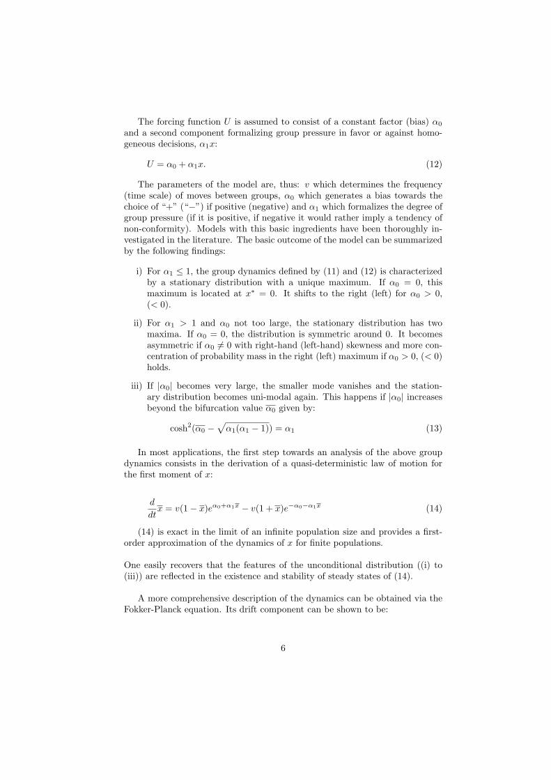
Table 3 shows our results exhibiting the mean estimates, finite sample stan-dard errors and root-mean squared errors for all underlying parameters. Themain message is that we can estimate the parameters v, α0 and α1 quite ac-curately even for our relatively small sample of 200 observations. In all cases,the Crank-Nicolson estimates are by far better than those obtained on the baseof the Euler approximation, in terms of bias and standard error. One also in-fers that estimated parameters become somewhat less reliable in the cases ofparameter sets II and IV as compared to I and III, respectively. The reason isprobably that a positive bias interferes with the effects of interaction so that thevariability of estimated parameters across samples increases. Nevertheless, theoverall bias and standard error still remain reasonable even in those cases withα0 = 0.2 (with the exception perhaps of the estimates of v for parameter setIV). In contrast, Euler estimates appear essentially useless in these cases. Asconcerns the influence of the density of the grid, we observe only minor differ-ences between the Crank-Nicolson approximations with k = 1

8 and k = 116 .

In fact, results do not uniformly improve when reducing the time increments:while one obtains slight improvements for the parameters α0 and α1, the esti-mates of v seem to deteriorate. The near equivalance of both settings togetherwith seemingly reasonable biases and standard errors suggests the conclusionthat using finer grids would probably not improve significantly the quality ofthe parameter estimates.

Another set of Monte Carlo experiments is motivated by realizing that thenumber of agents (the system size) N appears as a variable in the diffusionpart of the Fokker-Planck equation. Neglecting the issue of discreteness of N ,we can, in principle, also use our approach to arrive at an estimate of thenumber of active agents instead of imposing a predetermined value of N . Inour pertinent Monte Carlo experiments, we use again parameter sets I and IV(i.e. a symmetric setting with weak herding and an asymmetric one with strongherding), with N = 50 or N = 500 in both cases. The results are exhibited inTable 4... (to be added)

10

Euler Crank-Nicolson Crank-Nicolson(k = 1) (k = 1/8) (k = 1/16)

v α0 α1 v α0 α1 v α0 α1

mean 0.999 -0.001 0.642 2.980 -0.000 0.793 3.023 -0.000 0.794set I FSSE 0.091 0.007 0.052 0.567 0.005 0.028 0.585 0.005 0.028

RMSE 2.003 0.007 0.166 0.564 0.005 0.028 0.583 0.005 0.028mean 0.439 0.578 0.123 2.992 0.216 0.772 3.547 0.211 0.782

set II FSSE 0.048 0.097 0.171 1.046 0.057 0.105 1.422 0.038 0.069RMSE 2.561 0.390 0.698 1.041 0.059 0.108 1.517 0.039 0.071mean 1.019 0.000 1.173 2.884 0.000 1.196 2.952 0.000 1.196

set III FSSE 0.126 0.024 0.034 0.457 0.009 0.015 0.499 0.009 0.015RMSE 1.913 0.024 0.043 0.469 0.009 0.016 0.499 0.009 0.015mean 0.232 1.741 -0.698 1.369 0.262 1.123 1.748 0.245 1.144

set IV FSSE 0.026 0.350 0.426 0.245 0.127 0.159 0.439 0.127 0.159RMSE 2.768 1.580 1.945 1.326 0.141 0.175 1.326 0.135 0.168

Table 3: Approximate ML Estimates: the table displays the mean parameterestimates over 200 Monte Carlo replications together with their finite samplestandard errors (FSSE) and root mean squared errors (RSME).

4 Estimation of Interactive Opinion Formation:The Case of the ZEW Business Climate Index

ν α0 α1 α2 N logL AIC BICModel 1 0.78 0.01 1.19 -726.9 1459.8 1464.1

(baseline) (0.06) (0.01) (0.01)Model 2 0.15 0.09 0.99 21.21 -655.9 1319.7 1322.0(end. N) (0.07) (0.06) (0.14) (9.87)Model 3 0.14 0.15 0.94 -1.09 19.55 -655.7 1321.5 1321.8

(feedback from i) (0.07) (0.17) (0.21) (2.55) (10.13)Model 4 0.13 0.09 0.93 -4.55 19.23 -650.4 1310.9 1311.1

(feedback from IP) (0.06) (0.07) (0.16) (2.53) (8.78)Model 5 0.04 0.45 -11.93 5.75 -654.2 1316.4 1318.7

(no interaction) (0.01) (0.12) (3.98) (1.59)

Table 5: Parameter Estimates for Stochastic Models of Interacting Agents. De-tails on the underlying models appear in the main text. The numbers in bracketsare standard errors of parameter estimates.

Since we have focused an a very simple interaction scheme, it is not obvi-ous that its structural features should be easily applicable to economic data.Weidlich and Haag (1983, c.5) and Kraft, Landes and Weise (1986) had pro-posed simple business cycle models with, for example, investment decisions be-ing driven by an opinion process like the one outlined in Sec. 2. Such models

11

could be estimated using the above methodology. We leave this more demand-ing multi-variate application to future research and turn to a particular typeof uni-variate time series in which interaction effects could arguably play somerole. Various surveys for business climate or sentiment are regularly conductedin many countries that seem to receive much more attention by the publicthan by academic researchers. The leading examples are the Michigan Con-sumer Sentiment Index and the Conference Board Index for the U.S. economy,which have been reported monthly since the end of the 70ties (Ludvigson, 2004,Souleles, 2004). In Germany, similar surveys are conducted by the Ifo Institute(Ifo Business Climate Index) and the Center for European Research (ZEW) atthe University of Mannheim (denoted the ZEW Index of Economic Sentiment).Among these indices, the ZEW Sentiment index comes closest to the simplestructure of our ’canonical’ model in that it very literally asks for wether re-spondents are optimistic ( “+”) or pessimistic (“-”) concerning the prospectsof the German economy over the next six months. The only difference to ourmodel is that ZEW also allows for a neutral assessment. We might assume thatneutral subjects can be assigned half and half to the optimistic and pessimisticcamp which, then, would allow us to apply our model directly to their data.The index is, in fact, reported as the percentage of optimists minus pessimistsso that it can be directly used as the opinion index x introduced in Sec. 2. Incontrast, the indices for the U.S. economy are computed as weighted averagesover categorial answers to different questions while Ifo starts with sector-specificsurveys and aggregates them to an overall business climate indicator. The ZEWindex is, therefore, probably the only one that delivers us with an aggregate ofvery pure binary (resp., ternary) assessments. Fig. 2 displays the entire avail-able monthly ZEW series (starting in December 1991 and running through July,2006). Despite quite a number of differences in the data collection process, itsdevelopment is broadly parallel to that of the Ifo index. What is striking is thevery pronounced cyclical behavior of the ZEW index with very sudden move-ments upward and downward and a certain stagnation at times at a high orlow plateau. One could, in fact, argue that the dynamics of the ZEW index isreminiscent of a bi-modal stochastic dynamics switching between a high positiveand a moderately negative equilibrium. It might be worthwhile to contrast thisseries with what it is designed to predict, the cyclical component in economicactivity. This cyclical component appears in the lower panel of Fig. 2 in theform of residuals of monthly industrial production from the Hodrick-Prescottfilter, which is widely seen as the state-of-the-art approach for disentanglingtrend components and cyclical components in economic activity. Somewhatsurprising, the perception of the business cycle dynamics as reflected in the sur-vey allows a much more clear cut categorization of its phases than the muchmore random nature of filtered IP.

The ZEW surveys are based on about 350 respondents so that we mighttake this information as a parametric restriction on N (assuming N=175). We,then, have to estimate the parameters v, α0 and α1 in a baseline application ofour interacting-agents framework. Results are shown in Table 5. Interestingly,

12

the crucial parameter α1 is significantly larger than unity indicating bi-modalityof the limiting distribution. Despite the impression of a dominance of positiveassessment over the whole sample period (quite in contrast to stereotypes ofGerman “angst”) the bias term α0 turns out to be not significantly differentfrom 0. Unfortunately, simulations of the estimated model show, that it mostlikely would get stuck within one mode over a time horizon of the length of oursample (176 observations) and would on average at most switch only once fromone mode to the other (cf. Fig. 3 and 5 below). Transitions between modesare governed by chance fluctuations and become more and more unlikely thehigher the number of agents. Vice versa, frequent switches would only occur fora relatively small size of the underlying population. In order to reconcile ourobservation of a relatively large number of apparent switches of the mood of therespondents with the ‘official’ system size of 350 respondents, we could arguethat the ‘effective’ system size is smaller than the official number. This wouldhappen if some respondents would actually move broadly synchronously andwould, therefore, nor act like independent agents. While we cannot check thisassertion due to the anonymity of the data, we could let the index itself speakon the underlying effective system size by adding N to the list of parametersestimated via approximate ML. This approach is somewhat similar to that ofa recent paper by Chen (2002) who argues that the relative extent of fluctua-tions of macroeconomic data is neither in agreement with a representative-agentframework nor with the assumption of a system size identical to the number ofindividuals or companies in an economy. On the base of simple stochastic mod-els, he argues that the relative deviation (the square of the means divided bythe variance of the data) yields an estimate of the implicit number of degrees offreedom. While this rough non-parametric approach somewhat surprisingly pro-vides us with µ2

σ2 ≈ 0.9, our parametric model arrives at an estimate of N ≈ 20(i.e. 40 independent agents or groups of agents). Note that this added flexibilityleads to a relatively large increase in the log likelihood and is preferred over thebaseline model by both the AIC and BIC criteria. As concern estimated param-eters, α0 still is insignificant, while the interaction coefficient falls marginallybelow 1 indicating uni-modality albeit with possibly large excursions into ex-treme configurations. Remarkably, the estimate of the parameter v decreasesfrom 0.78 to 0.15 when proceeding from model 1 to model 2. The likely reasonis that the first estimation would have to come up with a higher mobility of thepopulation (higher propensity to change opinion) in order to compensate for thestagnatory tendency of the larger imposed population of model 1.We have remarked in sec. 2 that our framework allows to incorporate exoge-nous effects on the opinion formation process. In order to do so we simply couldexpand the influence function U by introducing additional factors that could beof importance to the assessment of the business cycle by the respondents of thesurvey:

U = α0 + α1x + α2y (17)

Most naturally, y could be macroeconomic data of the same frequency itself(i.e. monthly), although our framework could also accommodate data of higher

13

or lower frequency. Two such macro feedbacks have been investigated in ourmodels 3 and 4: the interest rate (3 month FIBOR rate) and industrial pro-duction (HP filtered, as displayed in Fig. 2). Note that the direction of thefeedback is not predetermined in our model, i.e. α2 could turn out to positiveor negative. The outcome of the exercise shows that industrial production addsmore explanatory power than the inclusion of the interest rate: for the formerwe obtain a significantly negative coefficient together with lower values of theAIC and BIC criteria. For the interest rate, in contrast, the estimated coeffi-cient α2 is not significant and overall improvements compared to model 2 aresmaller. However, even for the preferred model 4, the improvement comparedto model 2 is much smaller than the increase in logL, AIC and BIC achieved byadding N as a free parameter (the step from model 1 to model 2). Furthermoreboth the inclusion of the interest rate and of industrial production have onlyvery negligible effects on the parameters of the interacting agent model. Whatis perhaps puzzling is the negative sign of the feedback effect from industrialproduction which is in contrast to a positive contemporaneous correlation ofabout 0.28 between both series. It appears to depict some type of ‘contrarian’behaviour: if the economic data is indicating a boom phase, our respondentsseem already forestall the subsequent overheating of the economy and the sub-sequent downturn and vice versa.We tried also whether we could get rid of interaction, but the results of thepertinent exercise (model 5) are not too plausible: a very large positive predis-position (α0 = 0.48) together with a small population (N = 6) and a low degreeof flexibility (v = 0.03) is needed to compensate for the missing interaction ef-fect. AIC and BIC rank this variant inferior to model 4.

14

Tab

le6:

Unc

ondi

tion

alm

omen

tsfr

om1.

000

Mon

teC

arlo

sim

ulat

ions

data

mod

els

12

34

5m

ean:

0.35

2-0

.588

0.34

90.

335

0.32

40.

368

(95%

)(-

0.63

1,-0

.405

)(0

.045

,0.

552)

(0.1

00,0.

517)

(0.0

35,0.

528)

(0.1

49,0.

540)

std.

dev:

0.37

00.

098

0.35

50.

376

0.38

40.

334

(95%

)(0

.068

,0.

185)

(0.2

51,0.

484)

(0.2

65,0.

508)

(0.2

93,0.

506)

(0.2

44,0

.429

)sk

ewne

ss:

-0.6

200.

615

-0.9

08-0

.932

-0.9

91-0

.900

(95%

)(0

.029

,1.6

85)

(-1.

880,

0.09

7)(-

1.77

8,-0.

068)

(-1.

878,

0.05

3)(-

1.76

4,-0

.054

)ku

rtos

is:

-0.4

280.

575

0.59

10.

390

0.54

00.

859

(95%

)(-

0.65

2,3.

717)

(-1.

322,

4.34

7)(-

1.30

8,3

.775

)(-

1.28

3,3.

296)

(-0.

869,

3.39

8)re

l.de

viat

ion:

0.90

549

.705

1.36

81.

116

1.03

01.

298

(95%

)(8

.706

,82

.360

)(0

.024

,4.

022)

(0.0

55,3.

418)

(0.0

22,2.

792)

(0.2

25,3.

238)

dist

ance

:0.

952

0.33

50.

333

0.29

70.

290

(95%

)(0

.899

,0.

986)

(0.2

55,0.

493)

(0.2

59,0.

462)

(0.2

20,0.

455)

(0.2

28,0.

378)

15

Table 7: Autocorrelations from 1.000 Monte Carlo simulations

modelsACF data 1 2 3 4 5

1 0.935 0.630 0.923 0.936 0.939 0.925(95 %) (0.456 0.963) (0.845 0.967) (0.876 0.969) (0.908 0.968) (0.881 0.956)

2 0.830 0.404 0.853 0.875 0.880 0.851(0.162 0.929) (0.715 0.936) (0.764 0.940) (0.820 0.934) (0.762 0.908)

3 0.709 0.266 0.789 0.816 0.819 0.780(0.013 0.890) (0.595 0.907) (0.658 0.913) (0.732 0.900) (0.661 0.859)

4 0.584 0.175 0.729 0.761 0.758 0.710(-0.080 0.857) (0.496 0.883) (0.556 0.886) (0.652 0.866) (0.561 0.809)

5 0.465 0.116 0.673 0.707 0.696 0.643(-0.133 0.820) (0.398 0.860) (0.467 0.863) (0.566 0.833) (0.477 0.759)

6 0.363 0.075 0.620 0.655 0.633 0.578(-0.171 0.784) (0.319 0.840) (0.382 0.841) (0.478 0.797) (0.391 0.710)

7 0.272 0.048 0.571 0.605 0.571 0.515(-0.188 0.747) (0.241 0.813) (0.313 0.822) (0.392 0.759) (0.301 0.658)

8 0.186 0.032 0.525 0.558 0.512 0.455(-0.197 0.703) (0.184 0.793) (0.246 0.801) (0.317 0.722) (0.226 0.611)

9 0.094 0.022 0.482 0.513 0.454 0.399(-0.213 0.668) (0.121 0.774) (0.190 0.782) (0.239 0.678) (0.153 0.568)

10 0.017 0.014 0.442 0.470 0.398 0.345(-0.220 0.631) (0.078 0.752) (0.133 0.760) (0.167 0.640) (0.079 0.519)

d 0.553 0.194 0.826 0.875 0.923 0.792(-0.343 0.978) (0.338 1.261) (0.351 1.266) (0.455 1.346) (0.290 1.221)

5 Some specification tests

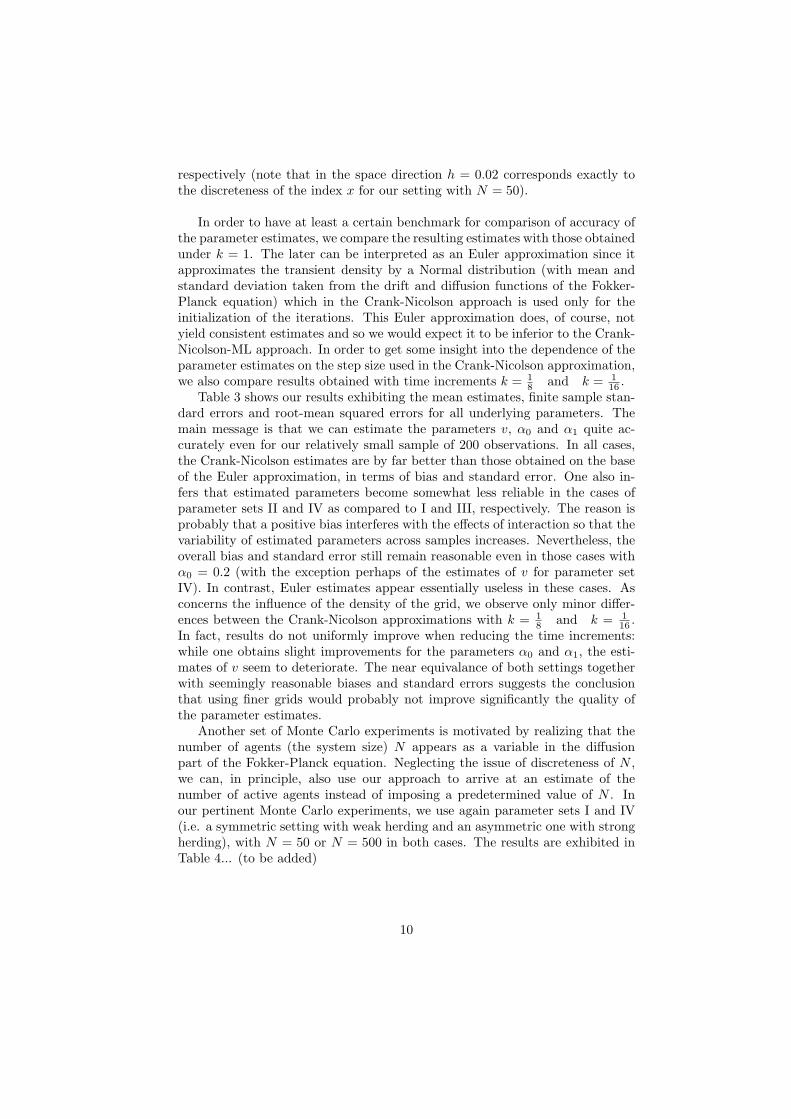
How close do time series from the estimated models get to empirical behavior ofthe ZEW index? Fig. 3 exhibits three simulations over the same time horizonof model 4 together with the empirical data. For these simulations, we haveused time increments ∆t = 0.01 for the ongoing opinion formation betweeninteger time steps and have injected the knowledge of the current exogenousfactor (HP-filtered industrial production) at integer time steps. As it can beseen, the visual appearance of the three Monte Carlo runs is pretty similar tothat of the index itself and the significant feedback from industrial productionseems to direct the simulations towards a pattern that is broadly synchronouswith the ups and downs of the empirical record. Fig. 4 shows the mean and95 percent confidence bounds from the transient density computed for model 4over the whole observation period given the first observation of the index as theinitial condition and incorporating the feedback from the news about industrialproduction. Since the empirical record stays within the 95 % bounds for practi-

16

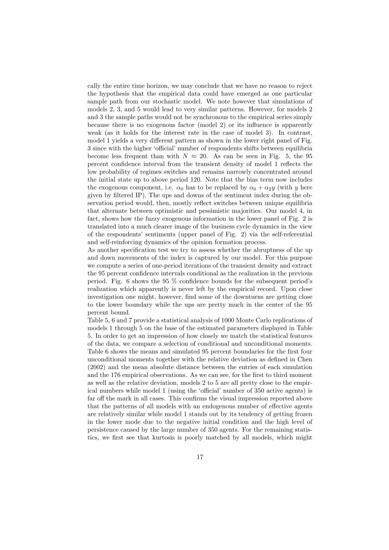
cally the entire time horizon, we may conclude that we have no reason to rejectthe hypothesis that the empirical data could have emerged as one particularsample path from our stochastic model. We note however that simulations ofmodels 2, 3, and 5 would lead to very similar patterns. However, for models 2and 3 the sample paths would not be synchronous to the empirical series simplybecause there is no exogenous factor (model 2) or its influence is apparentlyweak (as it holds for the interest rate in the case of model 3). In contrast,model 1 yields a very different pattern as shown in the lower right panel of Fig.3 since with the higher ‘official’ number of respondents shifts between equilibriabecome less frequent than with N ≈ 20. As can be seen in Fig. 5, the 95percent confidence interval from the transient density of model 1 reflects thelow probability of regimes switches and remains narrowly concentrated aroundthe initial state up to above period 120. Note that the bias term now includesthe exogenous component, i.e. α0 has to be replaced by α0 + α2y (with y heregiven by filtered IP). The ups and downs of the sentiment index during the ob-servation period would, then, mostly reflect switches between unique equilibriathat alternate between optimistic and pessimistic majorities. Our model 4, infact, shows how the fuzzy exogenous information in the lower panel of Fig. 2 istranslated into a much clearer image of the business cycle dynamics in the viewof the respondents’ sentiments (upper panel of Fig. 2) via the self-referentialand self-reinforcing dynamics of the opinion formation process.As another specification test we try to assess whether the abruptness of the upand down movements of the index is captured by our model. For this purposewe compute a series of one-period iterations of the transient density and extractthe 95 percent confidence intervals conditional as the realization in the previousperiod. Fig. 6 shows the 95 % confidence bounds for the subsequent period’srealization which apparently is never left by the empirical record. Upon closeinvestigation one might, however, find some of the downturns are getting closeto the lower boundary while the ups are pretty much in the center of the 95percent bound.Table 5, 6 and 7 provide a statistical analysis of 1000 Monte Carlo replications ofmodels 1 through 5 on the base of the estimated parameters displayed in Table5. In order to get an impression of how closely we match the statistical featuresof the data, we compare a selection of conditional and unconditional moments.Table 6 shows the means and simulated 95 percent boundaries for the first fourunconditional moments together with the relative deviation as defined in Chen(2002) and the mean absolute distance between the entries of each simulationand the 176 empirical observations. As we can see, for the first to third momentas well as the relative deviation, models 2 to 5 are all pretty close to the empir-ical numbers while model 1 (using the ‘official’ number of 350 active agents) isfar off the mark in all cases. This confirms the visual impression reported abovethat the patterns of all models with an endogenous number of effective agentsare relatively similar while model 1 stands out by its tendency of getting frozenin the lower mode due to the negative initial condition and the high level ofpersistence caused by the large number of 350 agents. For the remaining statis-tics, we first see that kurtosis is poorly matched by all models, which might

17

however be attributed to the volatility of this measure for small samples. Thedistance between the empirical observations and synthetic data again shows thegreatest discrepancy for model 1 compared to all others while the feedback fromindustrial production in models 4 and 5 seems to have contribute to a better fitcompared to models 2 and 3. Again, this provides a confirmation of our visualimpression reported above.Table 7 reports autocorrelations of the simulated series for lags 1 to 10. Aglance at smaller lags again indicates that ACFs from models 2 to 5 are all veryclose to their empirical counterpart while model 1 has a much lower degree ofdependence. Unfortunately, all models are only able to match about the firstfour lags while the autocorrelations remain much higher than the empirical onesfor the longer lags.

18

References

Aoki, M., New Approaches to Macroeconomic Modeling: Evolutionary StochasticDynamics, Multiple Equilibria, and Externalities as Field Effects, Cambridge,University Press 1996

Chen, P., Microfoundations of Macroeconomic Fluctuations and the Laws ofProbability Theory: The Principle of Large Numbers versus Rational Expec-tations Arbitrage, Journal of Economic Behavior and Organization 49, 2002,307-326

Jensen, B. and R. Poulsen, Transition Densities of Diffusion Processes: Nu-merical Comparison of Approximation Techniques, Journal of Derivatives 2002,18-34

Hurn, A., J. Jeisman and K. Lindsay, Teaching an Old Dog New Tricks Im-proved Estimation of the Parameters of Stochastic Differential Equations byNumerical Solution of the Fokker-Planck Equation, Manuscript,Queensland University of Technology, Brisbane 2006

Kraft, M.,T. Landes and P. Weise, Dynamic Aspects of a Stochastic BusinessCycle Model, Methods of Operations Research 53, 1986, 445-453

Ludwigson, S., Consumer Confidence and Consumer Spending, Journal of Eco-nomic Perspectives 18, 2004, 29-50

Lux, T., Herd Behaviour, Bubbles and Crashes, Economic Journal 105, 1995,881-896

Lux, T., Time variation of second moments from a noise trader/infection model,Journal of Economic Dynamics and Control 22,1997, 1-38

Souleles, N., Expectations, Heterogeneous Forecast Errors, and Consumption:Micro Evidence from the Michigan Consumer Sentiment Surveys, Journal ofMoney, Credit and Banking 36, 2004, 39-72

Poulsen, R., Approximate Maximum Likelihood Estimation of Discretely Ob-served Diffusion Processes, Manuscript, University of Aarhus, 1999.

Østerby, O.,The Error of the Crank-Nicolson Method for Linear Parabolic Equa-tions with a Derivative Boundary Condition, Manuscript, Universityof Aarhus, 1998

Giuliani, P., Fully Implicit and Crank-Nicolson Methods, Manuscript, Universityof St. Andrews

19

Thomas, J., Numerical Partial Differential Equations, Berlin, Springer 1995

Frank, T., Nonlinear Fokker-Planck Equations, Berlin, Springer 2005

Risken, H., The Fokker-Planck Equation: Methods of Solutions and Applica-tions, Berlin, Springer 1989

Weidlich, W. and G. Haag, Concepts and Methods of a Quantitative Sociol-ogy, Berlin, Springer 1983

Park, B. and V. Petrosian, Fokker-Planck Equations of Stochastic Accelera-tion: A Study of Numerical Methods, Astrophysical Journal Supplement 103,1996, 255

Weidlich, W., Sociodynamics: A Systematic Approach to Modeling in the SocialSciences. London, Taylor & Francis, 2002.

20

Figure 1: An illustration of the development of the transient density in thebimodal case. The initial state x0 has been approximated by a Normal distri-bution with small standard deviation and mean x0.

21

Figure 2: ZEW Sentiment Index and Industrial Production.

22

Figure 3: Simulated Trajectories from Models 4 and 1 (lower right-hand panel.)

23

Figure 4: Mean and 95 Percent Confidence Interval for Model 4 (from Fokker-Planck Equation)

24

Figure 5: Mean and 95 Percent Confidence Interval from Model 1 (from Fokker-Planck Equation)

25

Figure 6: 95 Percent Confidence Interval for One-Step Iterations of TransientDensity of Model 4.

26