Parallelism in Simulation and Modeling of Scale-Free Complex Networks

Tomas Hruza,∗, Stefan Geisselera, Marcel Schongensa

aInstitute of Theoretical Computer Science, ETH Zurich, Universitatstrasse 6, 8092 Zurich, Switzerland

Abstract

Evolution and structure of very large networks has attracted considerable attention in recent years. Inthis paper we study a possibility to simulate stochastic processes which move edges in a network leadingto a scale-free structure. Scale-free networks are characterized by a ”fat-tail” degree distribution withconsiderably higher presence of so called hubs - nodes with very high degree. To understand and predictvery large networks it is important to study the possibility of parallel simulation. We consider a class ofstochastic processes which keeps the number of edges in the network constant called equilibrium networks.This class is characterized by a preferential selection where the edge destinations are chosen according toa preferential function f(k) which depends on the node degree k. For this class of stochastic processeswe prove that it is difficult if not impossible to design an exact parallel algorithm if the function f(k) ismonotonous with an injective derivative. However, in the important case where f(k) is linear we present afully scalable algorithm with almost linear speedup. The experimental results confirm the linear scalabilityon a large processor cluster.

Keywords: scale-free networks, stochastic processes, nongrowing complex networks

1. Introduction

The study of complex networks has attracted considerable attention in recent years. The researchcommunity as well as the public has became sensitive to the fact that various sorts of networks haveprofound effect on our lives. We understand today that our brains, our communication lines, our highways,our flight connections and our social contacts (just to mention few examples) exhibit a structure of a complexnetwork with nodes representing the entities and edges representing some sort of interactions among them.Proliferation of networks has led to a deeper research showing that the behavior and the growth of suchnetworks are far from being purely random. It often follows certain topological and structural patternsdiscovered in the theory of scale-free networks and small worlds [1, 10, 18, 21, 7]. Scale-free networks arecharacterized by a ”fat-tail” degree distribution with considerably higher presence of so called hubs - nodeswith very high degree. Exactly speaking only the degree distribution P (k) = αk−γ , where P (k) denotesthe probability of finding a vertex with degree k in the network, is invariant under scaling. However, allnetworks having a log-log near linear degree distribution for higher degree k are studied under the termscale-free networks.

Stochastic processes are often used to model the evolution of complex networks. Such processes consistof simple phenomenological rules describing how the edges and nodes appear and change in the network.A master equation is a difference (or differential) equation describing the behavior of a certain networkquantity under the given stochastic process. The basic quantity characterizing the complex network is thedegree distribution. Degree distribution P (k, t) is the probability that at any given time t a vertex chosenuniformly at random would have degree equal to k.

∗Corresponding author.Email address: tomas.hruz@inf.ethz.ch (Tomas Hruz)

Published in Parallel Computing, 36(8):469-485, 2010, doi:10.1016/j.parco.2010.04.004

Figure 1: (color online) Illustration of the ”Simple Edge Selection Process” (SESP - see Process 1). The process selects an edgeuniformly at random (Picture A) and rewires it to a node which was preferentially selected (Picture B). A detailed explanationof preferential selection and the process definition is provided in Section 2. The rewiring is unconditional, this means that thereis no test of the connectivity state between vl and vj . During the rewiring operation the following three cases can occur: i)there is no edge between the node vl and the node vj , therefore the process does not create a multiple edge or a self loop, ii)there are already one or more edges between vl and vj , the process adds another edge between the nodes, and iii) if vl = vj ,the process creates a self-loop.

However, even the simplest edge and vertex change rules can lead to very complicated master equation[13]. In this situation a simulation of the network stochastic process can bring valuable insight into thebehavior and possible solutions of the master equation. Moreover, some real networks are so large andcomplicated that the only chance to setup a framework where they could be understood is to simulate themon a large scale.

For some critical networks like Internet it can be necessary in future to have an online prediction modelwhich would follow and predict the development of the network conditions. Similarly as the weather forecastservice observes, simulates and predicts the behavior of the atmosphere on earth it will be important to knowthe state and the future development of the network. In such applications fast parallel algorithms capable ofsimulating the network processes on a very large scale are needed. The network simulation systems can alsoplay a central role in understanding and preventing security problems in large networks. Fast simulationsof very large networks can show how the evolution of the underlying network structure influences the speedand other factors of a security problem spreading over the network.

To understand and predict very large networks it is important to study the possibility of parallel simula-tion. We concentrate on a basic building block of network evolution called preferential selection because itcreates a major obstacle to parallelization of scale-free models. Preferential selection denotes a step where anetwork node is selected with a probability dependent on its degree. This dependency is expressed througha preference function which we discuss in detail in the next sections. It is a part of larger step calledpreferential attachment, where after the node is preferentially selected an edge is attached to it which wasselected during the earlier stages of the stochastic process. We prove a theorem indicating that it will bevery hard (if not impossible) to find efficient and exact parallel algorithms for the general case. However, avery important special case of linear preferential attachment (for the discussion on importance of the linearcase see e.g. [11]) can be simulated in parallel and we provide an algorithm which achieves almost linearspeed-up in the number of processors.

The principal problem, under which conditions the stochastic processes generating scale-free networkscan be parallelized, was not studied in the literature. The authors in [22] consider a problem how to generatein parallel a large scale-free network which can be used for testing purposes of simulation frameworks. Theproposed method serves perfectly well for the purposes the authors in [22] consider, however the conditions onthe preference function which would allow resp. not allow efficient parallelization are not studied. Moreover,

2

in comparison to the method presented here, the PBA method from [22] can be used only for one particularpreference function f(k) = k, because selecting an edge uniformly at random and choosing its vertexin random is equivalent to the preference function f(k) = k. Our parallel algorithm allows to considerany linear preference function. The authors in [22] also develop a method called PK which provides adeterministic construction of scale-free graphs, however the stochastic process generating the graph is notprovided. We think that to identify this process a new research into equivalence between certain class ofstochastic processes and prescribed scale-free graphs would be needed. It is known that any prescribeddegree distribution in a graph can be achieved under the configuration model [18].

The class of complex networks similar to our scenario which was considered from the parallelism point ofview are small-world networks. Parallel algorithms for generation of small-world networks has been studiedin [2, 15]. Small-world networks have similar features as scale-free networks (for example small diameter)but the generating stochastic processes do not use preferential selection which is the main obstacle to theparallelization of scale-free networks as we argue below. Another field which can be related to our researchis the study of parallelism for Monte Carlo methods [23]. Intuitively, a stochastic process acting on anetwork can be transformed to a Monte Carlo setting, because the behavior of very large networks can becontinuously approximated with partial differential equation [10], where the degree plays a role of spatialcoordinate and discrete time is approximated with continuous time coordinate. However, to understand thisrelation and its consequences to parallel simulation of scale-free networks, a new branch of research wouldbe needed.

The stochastic process which we study in this paper provides a simplification of the processes occurringin real complex networks. The complex network community has proposed more complex processes to modelfiner phenomena (apart from scale-free degree distribution) occurring in real networks [5, 8]. However, forsuch stochastic processes a very limited body of theory exists which would provide a sufficient theoreticalanalysis (mean-field model) of their behavior not to say an analysis of their parallelization possibilities. Moststudies provide simulation results of proposed models which often illustrate that the model can capture thefeatures of real complex networks. Moreover, in many proposed processes, preferential attachment is used asa building block. This is also true for emergent studies of features like network conductivity [17] where thepreferential attachment plays a role of an important building block which is combined with other stochasticrules to obtain a conductivity modeling for Internet graphs. Therefore, a deeper study of the preferentialattachment provided in our paper can serve as a starting point to consider more complex scenarios.

Generic simulation systems like [9] can be succesfully build on an idea that in many situations even ifthe preferential selection is used, approximate solutions are possible. This is for example the case of sparsenetworks where our theory does not provide a good prediction. Another such case is discussed in concludingsection where we propose to use the linear approximation of weak non-linearities of preferential function.However, our analysis in Section 3 shows that in dense graphs with nonlinear preferential selection if exactsolution is needed the preferential selection is an obstacle for an efficient parallelism. In this case the focusshould be on parallely efficient and theoretically well understood approximations to the given stochasticprocess.

The present paper is organized as follows. In the next section we define the basic network generatingprocesses and the related notation. In Section 3. we study the depth of the dependency tree for generalpreferential attachment, and in Section 4 we provide a parallel algorithm for the linear preferential selection.We conclude with experimental results and possible directions of further research.

2. Stochastic Models of Complex Network Evolution

To model the nodes and the relations of a complex network we consider a multigraph G(V, E) withoutan orientation, where V is a set of nodes (vertices) and E is a set of edges. The number of nodes is denotedwith N , |V | = N and the number of edges with L, |E| = L. The basic quantity describing the networkevolution is the degree distribution defined as P (k) = N(k)/N , where N(k) denotes the number of nodeshaving degree k. The averaging of a quantity X is denoted with 〈X〉 or with X. Specifically, the averagedegree of the network is denoted with k, and it equals k = 2L/N . In the cases where we consider changesof the quantities like P (k) or N(k) over time, we add the parameter t as in N(k, t) or P (k, t).

3

Figure 2: (color online) Illustration of Process 2 - growing scale-free network. The process adds a new node to the existingnetwork (Picture A) and preferentially selects a node from the existing network, which is then connected to the new node(Picture B).

The complex network theory recognizes two principal cases with respect to the evolution of the numberof edges. First, there are non-growing or equilibrium networks where the number of edges L is constant orbounded within some interval. Second, growing or non-equilibrium networks are studied, where during thenetwork evolution the number of nodes and the number of edges grows substantially and it is not boundedby any constant.

In Process 1 we define a widely studied basic equilibrium process [10, 11, 13]. We call the processillustrated in Figure 1 ”Simple Edge Selection Process” (SESP). One repetition of the process steps calleda process loop models one discrete time unit. As an initial condition we generally suppose a multigraphG(V, E) with L edges and N vertices.

Process 1 SESPRequire: a multigraph G(V, E) with L edges and N vertices.1: Ns ⇐ StepLimit Initialize the number of process loops.2: while number of process loops smaller than Ns do

3: An edge, denoted Ei, is selected uniformly at random.4: An end vertex, denoted vi, of Ei is selected uniformly at random. The other end vertex will be denoted

as vj .5: A vertex, denoted vl, is selected with a probability proportional to f(k) i.e. with probability

f(k)/(N〈f〉) where k is the degree of vl.6: The edge Ei is rewired from vi to vl i.e. the edge Ei between vi and vj is deleted and a new edge

between vl and vj is created.7: end while

Non-growing complex networks have been observed in many situations. A typical example is representedby metabolic networks in living organisms which consist of complex chains of biochemical reactions inthe living cell [20, 14]. The number of reactions and substances flowing through the network is constant,however the network is stochastically changing its topology as a reaction to the changes of the organismstate. Another example are neural networks in brain where the activity of the connections between neuronsare stochastically reconfigured on the fly to reflect the current processing needs. An overview of furtherexamples together with modeling theory can be found in [19]. Generally, most of the growing networks(like for example Internet and WWW) will reach a saturation phase because of constraints on resources andenergy which are present in any physical system. Then the stochastic reconfiguration processes will prevail

4

over the growth processes.Step 5 in Process 1 is called preferential selection, and f(k), k ≥ 0 is a preference function. This is a basic

building block of processes generating scale-free distributions, which are the subjects of study in the theoryof complex networks. During the preferential selection a node is chosen in dependence of its degree. If thefunction f(k) is increasing, the nodes having more edges are chosen with higher probability. For example inthe case of Internet Web pages the authors are linking pages of their web sites to other pages already wellknown to them and these are exactly the web pages having already a lot of links. This sort of preferentialselection is often modeled with the linear preference function f(k) = βk+k0. On the other hand, to considernonlinearities in f(k) will be necessary if we want to have more accurate models of real networks, becausethere are natural constrains (on energy and other resources) which must lead to saturation effects. We

denote as 〈f〉 the mean value of f(k) which is generally dependent on time 〈f〉(t) =∑2L

s=0 f(s)P (s, t).The preferential selection is difficult to parallelize because it depends on global information, namely on

the development of the degree distribution. Closer inspection of the preferential selection suggests that aprocessing unit needs the whole information about the degree distribution whenever it wants to computethe selection probability s(k) = f(k)/(N〈f〉). Indeed, we can prove in Section 3 that this is the casefor a considerable range of scale-free networks with nonlinear preference function. Our idea of a parallelalgorithm for linear preference is based on the observation that we can replace the step dependent on thedegree distribution with steps where objects are chosen uniformly at random. This makes the process lessdependent on the information that can not be distributed cheaply across the processing units. On the otherhand, Steps 3 and 4 of Process 1 have a different character, independent of the degree distribution, thereforethey can be better parallelized. For example, the edges can be distributed between the processors, and arandomly chosen processor can uniformly at random choose an edge from the set of its local edges.

Master equation describes the time evolution of the degree distribution in the mean-field approximation[4]. It is a deterministic finite difference equation (or in some cases partial differential equation) whichdescribes the development of degree distribution mean value. For Process 1 the master equation [13, 10] canbe formulated as

P (k, t+1)=P (k, t)−f(k)

N〈f〉(t)P (k, t) +

f(k − 1)

N〈f〉(t)P (k−1, t) −

k

NkP (k, t) +

k + 1

NkP (k+1, t) + O(1/N2) (1)

where O(1/N2) denotes the terms dependent on 1/N2 which disappear very quickly for larger networks.As we illustrated in Figure 1 the SESP process can create multiple edges and self-loops, therefore we

need multigraphs as an underlying model. Because in the large graph limit the frequency of such artifactstends to zero [10], the multigraph setting is standardly used. On the other hand, it would be desirable tohave a model allowing only simple edges and no self-loops. In [13] we investigated the constraints preservingthe simple graph structure, and we have shown that the understanding of these constraints involves a wholehierarchy of object distributions, which makes the exact modeling very difficult.

The preferential selection constitutes an important building block for modeling of complex networks.This can illustrated on another much investigated class of complex networks that describes non-equilibriumresp. growing networks [3, 4]. The basic model of complex network growth is illustrated in Figure 2. Thestochastic process called ”Barabasi-Albert Model” (BM) can be defined with the following steps, where theinitial condition is again a multigraph G(V, E) with L edges and N vertices. Marginally, it can be notedthat this process does not create any new multiple edges and self-loops i.e. it preserves the simple graphproperty if the initial configuration is a simple graph.

5

Process 2 BMRequire: a multigraph G(V, E) with L edges and N vertices.1: Ns ⇐ StepLimit Initialize the number of process loops.2: while number of process loops smaller than Ns do

3: A vertex, denoted vi, added to the existing graph G.4: A vertex, denoted vj , is selected with a probability proportional to f(k) i.e. with probability

f(k)/(N〈f〉) where k is the degree of vj .5: A new edge Ei is created from vi to vj .6: end while

The master equation for BM can be formulated [10] as

N(k, t + 1) = N(k, t) +k − 1

tkN(k − 1, t) −

k

tkN(k, t) + δk,1 (2)

where t means discrete time starting at t = 2 and δk,1 is the Kronecker delta. In the basic setting theinitial condition is a graph having 2 vertices and one edge between them, i.e. N(k, 2) = 2δk,1.

In the rest of the paper we concentrate on the preferential selection step in the context of Process 1(SESP), however the analysis and the parallelization we propose are also applicable for other cases wherethe preferential selection is used.

3. Parallelism for General Preferential Selection

To show that parallel simulation is difficult in certain situations we proceed in three steps. In the firstpart we show that if the preference function f(k) is monotonous and has an injective derivative then theselection probability s(k) = f(k)/(N〈f〉) changes for every node in the the network if the degree distributionP (k, t) changes during a discrete time unit (process loop) of Process 1. In other words, to know the selectionprobability the information about all nodes in the network is necessary. To obtain this fact one has to followthe ⇒ direction of Lemma 3 and ⇒ direction of Lemma 4. Lemmata 1 and 2 are technical tools which arevalid for any preference function f(k). On the other hand to obtain Lemma 3 we have to suppose that thedifference (derivative) of the function f(k) is injective. For Lemma 4 to be valid a monotonous functionf(k) is necessary.

In the second part we additively suppose that the network distribution is bounded from above by ascale-free distribution. Under this condition we show in Theorem 6 that the degree distribution P (k, t)changes with high probability in every time unit of the Process 1. To prove Theorem 6 we need Lemma 5which is independent on any concrete degree distribution class. Now combining Lemmas 1 - 5 and Theorem6 we obtain a class of networks, namely the scale-free networks with monotonous nonlinear function f(k),for which the selection probability s(k) changes with high probability in every time unit for all nodes in thenetworks.

In the third part we develop a model of parallel computing which considers dependencies between compu-tation states based on changes in degree distribution. The idea (captured in the definition of the dependencytree) is to organize the computational states in a tree where the edges model the dependencies of the selec-tion probability on degree distribution. We summarize our analysis in Theorem 7 about the depth of thedependency tree during the simulation of Process 1.

Additionally we use the following notation. Let [a, b] denote the interval of integers n such that a ≤ n ≤b. We denote the degree of node i in discrete time t of Process 1 by ki(t). Observe, that in each step of theprocess the connectivity of at most two vertices vi and vl is changed. By K = ki(t), kl(t), ki(t + 1), kl(t + 1)we denote the degrees that get changed in step t and t + 1. The following Lemma reveals an importantconnection between these degrees and the development in the degree distribution.

6

Lemma 1. For every discrete time t of Process 1 the following equivalence holds:

vi = vl ∨ ki(t) = kl(t) + 1 ⇔ ∀k ∈ [0, 2L] : P (k, t + 1) = P (k, t) .

Proof. First we consider ⇒: If vi = vl, then ki(t) 6= kl(t) + 1. Since from vi = vl it follows directly that∀k ∈ [0, 2L] : P (k, t + 1) = P (k, t), we only need to consider the case when ki(t) = kl(t) + 1. We decomposethe process into two phases. Phase one is the deletion of the edge (vj , vi) and phase two is the adding ofedge (vj , vl). Moreover, N(k, t), N(k, t + 1) only differ in k ∈ K. We do not consider vertex vj since nochange is caused in any of the two phases. In the first phase vi moves from the set of vertices with degreeki(t) to the set of vertices with degree ki(t) − 1 = kl(t). We denote the state after phase one and beforephase two by t′. We obtain

N(ki(t), t′) = N(ki(t), t) − 1

N(kl(t), t′) = N(kl(t), t) + 1 .

For phase two the only thing that happens is that vertex vl moves from the set of vertices with degree kl(t)to the set of vertices with degree kl(t) + 1 = ki(t). Then,

N(ki(t), t + 1) = N(ki(t), t′) + 1

N(kl(t), t + 1) = N(kl(t), t′) − 1 .

Therewith, we get that N(ki(t), t + 1) = N(ki(t), t) and N(kl(t), t + 1) = N(kl(t), t). From the fact thatki(t + 1) = ki(t) − 1 = kl(t) and kl(t + 1) = kl(t) + 1 = ki(t) we also obtain that N(ki(t + 1), t + 1) =N(ki(t+1), t) and N(kl(t+1), t+1) = N(kl(t+1), t). Since P (k, t) = N(k, t)/N we have P (k, t+1) = P (k, t).

Now, we consider ⇐: Assume for the sake of contradiction, that vi 6= vl ∧ kl(t) + 1 6= ki(t). Considerdegree ki(t). In Phase 1 the edge (vj , vi) is removed, s.t. N(ki(t), t

′) = N(ki(t), t) − 1. In Phase 2 theedge (vj , vl) is added. If vi 6= vl we know that kl(t + 1) = kl(t) + 1. Since kl(t) + 1 6= ki(t) it followsthat kl(t + 1) 6= ki(t). That means that vl will not get a degree of ki(t) in discrete time step t + 1.Further, vl does not contribute to N(ki(t), t + 1). Hence, N(ki(t)) does not change in Phase 2 and wehave N(ki(t), t + 1) = N(ki(t), t

′) = N(ki(t), t) − 1. This is a contradiction, because we can derive thatP (ki(t), t) 6= P (ki(t), t + 1).

The next lemma studies the time development of the preference function mean during the process.

Lemma 2. Let f(k), k ≥ 0 be a preference function in Process 1. For any discrete time t it holds that

〈f〉(t + 1) − 〈f〉(t) =1

N(f(ki(t) − 1) − f(ki(t)) + f(kl(t) + 1) − f(kl(t))) .

Proof. By definition we obtain

〈f〉(t + 1) − 〈f〉(t) =

2L∑

k=0

f(k)P (k, t + 1) −

2L∑

k=0

f(k)P (k, t) .

As mentioned above, only the connectivity of vi and vl is changed and corresponding degrees are K =ki(t), kl(t), ki(t + 1), kl(t + 1). Hence,

〈f〉(t + 1) − 〈f〉(t) =1

N

(

∑

k∈K

f(k)N(k, t + 1) −∑

k∈K

f(k)N(k, t)

)

.

7

For N(k, t + 1) of the first sum, we get the following identities:

N(ki(t), t + 1) = N(ki(t), t) − 1

N(ki(t + 1), t + 1) = N(ki(t + 1), t) + 1

N(kl(t), t + 1) = N(kl(t), t) − 1

N(kl(t + 1), t + 1) = N(kl(t + 1), t) + 1 .

Therewith, the second sum can be subtracted directly, such that we obtain

〈f〉(t + 1) − 〈f〉(t) =1

N(f(ki(t + 1)) − f(ki(t)) + f(kl(t + 1)) − f(kl(t)))

=1

N(f(ki(t) − 1) − f(ki(t)) + f(kl(t) + 1) − f(kl(t))) ,

which completes our proof.

The following lemma is establishing the relation between changes in the degree distribution and thepreference function f .

Lemma 3. Let f(k), k ≥ 0 be a preference function in Process 1 for which the first difference ∆f(k) =f(k + 1) − f(k) is injective. Then the degree distribution does not change in one discrete time unit ofProcess 1 iff the mean 〈f〉 of f(k) does not change, i.e:

∀k ∈ [0, 2L] : P (k, t + 1) = P (k, t) ⇔ 〈f〉(t + 1) = 〈f〉(t). (3)

Proof. First, we show the direction ⇒ in (3). Given P (k, t + 1) = P (k, t) we have

〈f〉(t) =

2L∑

k=0

f(k)P (k, t) =

2L∑

k=0

f(k)P (k, t + 1) = 〈f〉(t + 1).

For the direction ⇐ in (3), let us suppose that 〈f〉(t + 1) = 〈f〉(t). If vi = vl we can conclude thatP (k, t + 1) = P (k, t) because the selected edge is detached from the vertex vi and immediately reattachedto the same vertex. For vi 6= vl we have 0 = 〈f〉(t + 1) − 〈f〉(t). By Lemma 2 the following equalities hold

0 =1

N(f(ki(t) − 1) − f(ki(t)) + f(kl(t) + 1) − f(kl(t))) =

1

N(∆f(kl(t)) − ∆f(ki(t) − 1)) .

Therefore, by injectivity of ∆f(k) we obtain:

0 = ∆f(kl(t)) − ∆f(ki(t) − 1) ⇒ ∆f(kl(t)) = ∆f(ki(t) − 1) ⇒ ki(t) = kl(t) + 1.

Finally, we can apply Lemma 1 to obtain the desired result.

The next step in understanding the obstacles in parallelization of the preferential selection is how changesin the mean 〈f〉 of the preference function influence the changes in the selection probability.

Lemma 4. Let f(k) ≥ 0, k ≥ 0 be a strictly monotonic (decreasing or increasing) positive preference func-tion in Process 1. If 〈f〉 changes in one discrete time unit of Process 1, then the selection probabilitys(k) = f(k)/(N〈f〉) changes for all vertices i.e.

∀vi ∈ V :f(ki(t + 1))

N〈f〉(t + 1)6=

f(ki(t))

N〈f〉(t)

Proof. Because we rewire only one edge from a vertex vi to a vertex vl in one discrete time unit of Process 1,the degree k and therefore f(k) can change for at most 2 vertices vi and vl. For all other vertices vm we

8

have km(t) = km(t + 1) and only 〈f〉 changes. Thus, the selection probability changes and we obtain

f(km(t))

N〈f〉(t)6=

f(km(t + 1))

N〈f〉(t + 1).

For the vertices vi and vl it remains to show that

f(ki(t + 1))

〈f〉(t + 1)6=

f(ki(t))

〈f〉(t)and

f(kl(t + 1))

〈f〉(t + 1)6=

f(kl(t))

〈f〉(t).

According to Lemma 3 the mean value 〈f〉(t) =∑2L

k=0 f(k)P (k, t) changes if and only if there exists a kfor which P (k, t) changes, therefore vi 6= vl (in Process 1 if vi = vl the degree distribution P (k, t) does notchange because the edge is reattached to the same vertex) and the graph contains at least 2 vertices.

For all vertices vm ∈ VN〈f〉 ≥ f(km) (4)

This can be seen as follows. Since f and P (k, t) are non-negative functions it follows that

N〈f〉 = N

2L∑

k=0

f(k)P (k, t) ≥ Nf(km)P (km, t) = f(km)N(km, t) ≥ f(km) ,

because vm ∈ N(km, t).Suppose that f(k) is increasing. From the proof of Lemma 1 we know that kl(t + 1) = kl(t) + 1. For

vertex vl using Lemma 2 we get

f(kl(t + 1))

〈f〉(t + 1)=

f(kl(t) + 1)

〈f〉(t + 1)=

f(kl(t) + 1)

〈f〉(t) + f(kl(t)+1)−f(kl(t))+f(ki(t)−1)−f(ki(t))N

.

It holds f(ki − 1) − f(ki) < 0 since f is strictly monotone increasing. Hence, we derive that

f(kl(t + 1))

〈f〉(t + 1)> N

f(kl(t)) + f(kl(t) + 1) − f(kl(t))

N〈f〉(t) + f(kl(t) + 1) − f(kl(t))= N

f(kl(t)) + c

N〈f〉(t) + c,

where c = f(kl(t) + 1) − f(kl(t)). Since inequality (4) N〈f〉 ≥ f(kl) allows to reduce the term removing c,it follows that

f(kl(t + 1))

〈f〉(t + 1)> N

f(kl(t))

N〈f〉(t)=

f(kl(t))

〈f〉(t).

Now we consider vertex vi. Analogically as above, using Lemma 2 we obtain

f(ki(t + 1))

〈f〉(t + 1)=

f(ki(t) − 1)

〈f〉(t + 1)=

f(ki(t) − 1)

〈f〉(t) + f(kl(t)+1)−f(kl(t))+f(ki(t)−1)−f(ki(t))N

.

Due to strict monotonicity of f it holds that f(kl + 1) − f(kl) > 0 and we get

f(ki(t + 1))

〈f〉(t + 1)< N

f(ki(t)) + f(ki(t) − 1) − f(ki(t))

N〈f〉(t) + f(ki(t) − 1) − f(ki(t))= N

f(ki(t)) + c

N〈f〉(t) + c

where c = f(ki(t) − 1) − f(ki(t)). As a result of inequality (4) we can finally derive

f(ki(t + 1))

〈f〉(t + 1)< N

f(ki(t))

N〈f〉(t)=

f(ki(t))

〈f〉(t).

9

Analogically for a decreasing positive function f(k) we obtain that

f(kl(t + 1))

〈f〉(t + 1)<

f(kl(t))

〈f〉(t)and

f(ki(t + 1))

〈f〉(t + 1)>

f(ki(t))

〈f〉(t).

Therefore the selection probability s(k) = f(k)N〈f〉 changes for all N vertices in G, when 〈f〉 changes.

Before we can prove Theorem 6 below, which describes how often (probabilistically) the degree distribu-tion changes for a scale-free network during the process, we need the following technical Lemma 5.

Lemma 5. Let G(t) = (V, E(t)) be a network. The probability that the degree distribution does not changein a single discrete time step of Process 1 is

Pr [∀k ∈ [0, 2L] : P (k, t) = P (k, t + 1)] =

2L∑

k=1

f(k)P (k)k

〈f〉2L+

2L∑

k=1

f(k − 1)P (k − 1)P (k)k

〈f〉〈k〉.

Proof. By Lemma 1 we get

Pr [∀k ∈ [0, 2L] : P (k, t) = P (k, t + 1)] ⇔ Pr [vi = vl ∨ ki(t) = kl(t) + 1] ,

and since Pr [vi 6= vj ∧ kl(t) + 1 6= ki(t)] = 0 (see the proof of Lemma 1) we obtain

Pr [∀k ∈ [0, 2L] : P (k, t) = P (k, t + 1)] = Pr [vi = vl] + Pr [ki(t) = kl(t) + 1] .

For the first probability we have

Pr [vi = vl] =2L∑

k=0

Pr [vi = vl | ki(t) = k] Pr [ki(t) = k] =2L∑

k=1

f(k)

N · 〈f〉

N(k)k

2L

since there are N(k) vertices each connected to k half edges, the probability of selecting a half-edge connectedto a vertex with degree k is Pr [ki(t) = k] = (N(k)k)/(2L). By Process 1 the probability of selecting vertexvl with degree k is (f(k)N(k))/(N〈f〉), but out of all N(k) vertices with degree k only one is vi, thusPr [vi = vl | ki(t) = k] = f(k)/(N〈f〉). Pr [ki(t) = 0] = 0 because vi is selected through an edge selection,therefore the summation can start from 1. By the same argument the second probability is

Pr [kl(t) + 1 = ki(t)] =

2L∑

k=0

Pr [kl(t) + 1 = ki(t) | ki(t) = k] Pr [ki(t) = k] =

2L∑

k=1

f(k − 1)N(k − 1)

N · 〈f〉

N(k)k

2L.

Therefore, the overall probability is

Pr [∀k ∈ [0, 2L] : P (k, t) = P (k, t + 1)] =

2L∑

k=1

f(k)

N · 〈f〉

N(k)k

2L+

2L∑

k=1

f(k − 1)N(k − 1)

N · 〈f〉

N(k)k

2L.

Since P (k) = (N(k))/N and the expected degree per vertex is 〈k〉 = (2L)/N , we get

Pr [∀k ∈ [0, 2L] : P (k, t) = P (k, t + 1)] =

2L∑

k=1

f(k)P (k)k

〈f〉2L+

2L∑

k=1

f(k − 1)P (k − 1)P (k)k

〈f〉〈k〉.

From Lemma 3 and 4 we know that if the distribution P (k, t) changes then the selection probability s(k)changes for all vertices. Now we want to know what is the probability that P (k, t) changes. To estimatethis probability we consider a class of networks for which the degree distribution is bounded from above by

10

a scale free function. We call a network G = (V, E) scale free for the parameters α ∈ R+ and γ > 1, if the

degree distribution is bounded by

Figure 3: (Color online) Illustration of bounding area for the pref-erence function f(k) in Theorem 6.

P (k) ≤

αk−γ for k ≥ 1

1 for k = 0.

This class of networks is in fact larger thanthe one usually understood under the term scale-scale. Moreover, we bound also the (nonlinear)preference function on the interval [0, 2L] to beinside a region illustrated in Figure 3. The regionis bounded from above by linear function β1k+β0

and from the bottom by β3k − β3. It is possibleto consider a larger class of functions f(k), butthis will make the proof more complex and wedo not believe it would bring substantially new

information. Under these assumptions we can bound from below the probability of a change in P (k, t) asfollows.

Theorem 6. Let G = (V, E) be a scale free network with parameters γ ≥ 2 and let f be a preference functionthat is bounded by a region defined as (see Figure 3)

f(k) ≤ β1k + β0, f(k) ≥

0 for k ∈ [0, 1)

β3k − β3 for k ≥ 1,

where β1, β3 > 0 and β0 ≥ 0. Then the probability that the degree distribution stays the same in one discretetime step is bounded by

Pr [∀k ∈ [0, 2L] : P (k, t) = P (k, t + 1)] ≤αβ1

β3〈k〉 − β3+

4αβ0 ln(2L)

2L [β3〈k〉 − β3]+

β0

〈k〉 [β3〈k〉 − β3]+

2α2 (β1 + β0)

〈k〉 [β3〈k〉 − β3].

Proof. Lemma 5 states that

Pr [∀k ∈ [0, 2L] : P (k, t) = P (k, t + 1)] =

2L∑

k=1

f(k)P (k)k

2L〈f〉+

2L∑

k=1

f(k − 1)P (k − 1)P (k)k

〈f〉〈k〉. (5)

Under the assumption that the network is scale free and that f(k) is bounded linearly, for the first summandwe get

∑2Lk=1 f(k)P (k)k

2L〈f〉≤

∑2Lk=1 (β1k + β0)αk−γk

2L∑2L

k=1 (β.k − β3)P (k)=

αβ1

∑2Lk=1 k2−γ + αβ0

∑2Lk=1 k1−γ

2L[

β3

∑2L

k=1 kP (k) − β3

∑2L

k=1 P (k)] .

By definition of∑2L

k=1 kP (k) = 〈k〉. We bound∑2L

k=1 P (k) from above by 1 and by the fact that γ ≥ 2, weobtain

∑2L

k=1 f(k)P (k)k

2L〈f〉≤

αβ12L + αβ0

∑2L

k=1 k−1

2L [β3〈k〉 − β3].

The harmonic series∑2L

k=1 k−1 converges against ln(2L) + γ where γ is the Euler–Mascheroni constant.

11

Thus, for all L ≥ 1 it holds that ln(2L) + γ < ln(2L) + 1. Consequently,

∑2Lk=1 f(k)P (k)k

2L〈f〉≤

αβ12L

2L [β3〈k〉 − β3]+

αβ0 (ln(2L) + 1)

2L [β3〈k〉 − β3]≤

αβ1

β3〈k〉 − β3+

4αβ0 ln(2L)

2L [β3〈k〉 − β3]. (6)

Analogously, for the second summand we get

∑2Lk=1 f(k − 1)P (k − 1)P (k)k

〈f〉〈k〉=

f(0)P (0)P (1) +∑2L

k=2 f(k − 1)P (k − 1)P (k)k

〈k〉∑2L

k=1 f(k)P (k)

≤β0 +

∑2Lk=2 (β1(k − 1) + β0)α(k − 1)−γαk−γk

〈k〉∑2L

k=1 (β3k − β3)P (k)

For γ ≥ 2 we get

∑2L

k=1 f(k − 1)P (k − 1)P (k)k

〈f〉〈k〉≤

β0 + α2∑2L

k=2 (β1(k − 1) + β0) (k − 1)−2k−1

〈k〉[

β3

∑2L

k=1 kP (k) − β3

∑2L

k=1 P (k)] .

Since k−1 is monotone decreasing, k−1 ≤ (k − 1)−1. Again, we bound∑2L

k=1 P (k) from above by 1. Byshifting the index of the sum, we obtain

∑2L

k=1 f(k − 1)P (k − 1)P (k)k

〈f〉〈k〉≤

β0 + α2∑2L−1

k=1 (β1k + β0) k−2k−1

〈k〉[

β3

∑2Lk=1 kP (k) − β3

]

=β0 + α2β1

∑2L−1k=1 k−2 + α2β0

∑2L−1k=1 k−3

〈k〉 [β3〈k〉 − β3].

It is∑∞

k=1 k−x ≤ 2 for any x ≥ 2 which yields

∑2L

k=1 f(k − 1)P (k − 1)P (k)k

〈f〉〈k〉≤

β0

〈k〉 [β3〈k〉 − β3]+

2α2 (β1 + β0)

〈k〉 [β3〈k〉 − β3]. (7)

Putting (6) and (7) into (5) yields

Pr [∀k ∈ [1, 2L] : P (k, t) = P (k, t + 1)] ≤αβ1

β3〈k〉 − β3+

4αβ0 ln(2L)

2L [β3〈k〉 − β3]

+β0

〈k〉 [β3〈k〉 − β3]+

2α2 (β1 + β0)

〈k〉 [β3〈k〉 − β3]

which completes the proof.

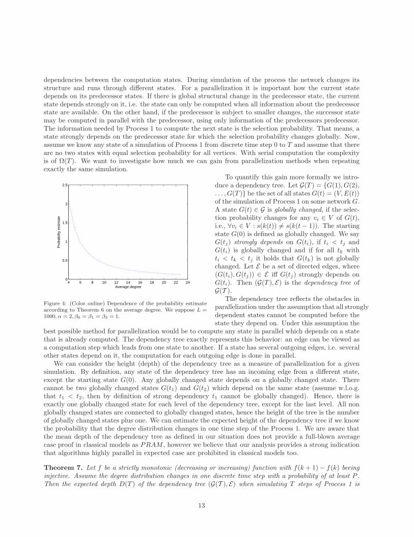
Let us consider what Theorem 6 means for networks observed in real situations. In [10] pp. 80 theauthors collected basic characteristics (average degree, γ etc.) from more than 30 real networks. In manyimportant cases like for example the Web, the average degree 〈k〉 is larger than 10 and L is much larger than1000. Already for a value of 1000 the second term in Theorem 6 is of order 10−2 therefore we can neglectthis term for most of real networks. In most of the cases γ ≥ 2. It is also reasonable to suppose a weaknonlinearity in f(k) therefore we can suppose β0 = β1 = β3 = 1. In Figure 4 we show how the probabilityin Theorem 6 depends on the average degree if we take the above assumptions. It is also clear from Figure 4that our estimate in Theorem 6 is not accurate enough for k ≤ 6 because probability can not be larger than1. We can conclude that for real networks with average degree larger than 8 the probability that degreedistribution changes is larger than 1/2.

To capture the problems in design of parallel simulation algorithms for network processes we consider

12

dependencies between the computation states. During simulation of the process the network changes itsstructure and runs through different states. For a parallelization it is important how the current statedepends on its predecessor states. If there is global structural change in the predecessor state, the currentstate depends strongly on it, i.e. the state can only be computed when all information about the predecessorstate are available. On the other hand, if the predecessor is subject to smaller changes, the successor statemay be computed in parallel with the predecessor, using only information of the predecessors predecessor.The information needed by Process 1 to compute the next state is the selection probability. That means, astate strongly depends on the predecessor state for which the selection probability changes globally. Now,assume we know any state of a simulation of Process 1 from discrete time step 0 to T and assume that thereare no two states with equal selection probability for all vertices. With serial computation the complexityis of Ω(T ). We want to investigate how much we can gain from parallelization methods when repeatingexactly the same simulation.

To quantify this gain more formally we intro-

4 6 8 10 12 14 16 18 20 22 240

0.5

1

1.5

2

2.5

Average degree

Pro

babi

lity

estim

ate

Figure 4: (Color online) Dependence of the probability estimateaccording to Theorem 6 on the average degree. We suppose L =1000, α = 2, β0 = β1 = β3 = 1.

duce a dependency tree. Let G(T ) = G(1), G(2),. . . , G(T ) be the set of all states G(t) = (V, E(t))of the simulation of Process 1 on some network G.A state G(t) ∈ G is globally changed, if the selec-tion probability changes for any vi ∈ V of G(t),i.e., ∀vi ∈ V : s(k(t)) 6= s(k(t − 1)). The startingstate G(0) is defined as globally changed. We sayG(tj) strongly depends on G(ti), if ti < tj andG(ti) is globally changed and if for all tk withti < tk < tj it holds that G(tk) is not globallychanged. Let E be a set of directed edges, where(G(ti), G(tj)) ∈ E iff G(tj) strongly depends onG(ti). Then (G(T ), E) is the dependency tree ofG(T ).

The dependency tree reflects the obstacles inparallelization under the assumption that all stronglydependent states cannot be computed before thestate they depend on. Under this assumption the

best possible method for parallelization would be to compute any state in parallel which depends on a statethat is already computed. The dependency tree exactly represents this behavior: an edge can be viewed asa computation step which leads from one state to another. If a state has several outgoing edges, i.e. severalother states depend on it, the computation for each outgoing edge is done in parallel.

We can consider the height (depth) of the dependency tree as a measure of parallelization for a givensimulation. By definition, any state of the dependency tree has an incoming edge from a different state,except the starting state G(0). Any globally changed state depends on a globally changed state. Therecannot be two globally changed states G(t1) and G(t2) which depend on the same state (assume w.l.o.g.that t1 < t2, then by definition of strong dependency t1 cannot be globally changed). Hence, there isexactly one globally changed state for each level of the dependency tree, except for the last level. All nonglobally changed states are connected to globally changed states, hence the height of the tree is the numberof globally changed states plus one. We can estimate the expected height of the dependency tree if we knowthe probability that the degree distribution changes in one time step of the Process 1. We are aware thatthe mean depth of the dependency tree as defined in our situation does not provide a full-blown averagecase proof in classical models as PRAM , however we believe that our analysis provides a strong indicationthat algorithms highly parallel in expected case are prohibited in classical models too.

Theorem 7. Let f be a strictly monotonic (decreasing or increasing) function with f(k + 1) − f(k) beeinginjective. Assume the degree distribution changes in one discrete time step with a probability of at least P .Then the expected depth D(T ) of the dependency tree (G(T ), E) when simulating T steps of Process 1 is

13

bounded from below by PT , i.e.,E [D(T )] ≥ PT .

Proof. If the degree distribution changes in one discrete time step with probability P , then by Lemma 3it holds that

Pr [∀kP (k, t) = P (k, t + 1)] = Pr [〈f〉(t) = 〈f〉(t + 1)] , (8)

if f(k + 1) − f(k) is injective. From Lemma 4 it follows for f beeing strictly monotonic (decreasing orincreasing) that

Pr [〈f〉(t) 6= 〈f〉(t + 1)] ≤ Pr [∀vi ∈ V : s(k, t) 6= s(k, t + 1)] , (9)

where s(k, t) = f(ki(t))/(N〈f〉(t)). Combining (8) and (9) with the premise that a change in the degreedistribution is bounded by P yields

P ≤ Pr [∀kP (k, t) 6= P (k, t + 1)] ≤ Pr [∀vi ∈ V : s(k, t) 6= s(k, t + 1)] .

This means, that the probability that the state at time step t + 1 is globally changed is not less than P .By definition of the dependency tree, any globally changed state sits on a new level since it is connected

to the direct predecessor state which is globally changed. That means the n-th globally changed state is atdepth n − 1, because the first state is globally changed and has depth 0.

Now we count the depth of the dependency tree by introducing a Bernoulli random variable bt with1 ≤ t ≤ T for any state G(t) of Process 1, which is 1 if G(t) is globally changed and 0 otherwise. Thus, the

depth of the dependency tree is D(T ) =∑T

t=1 bt. Then the expected depth is

E [D(T )] = E

[

T∑

t=1

bt

]

=

T∑

t=1

E [bt] ,

where E [bt] = Pr [bt = 1]. By (7) we have Pr [bt = 1] ≥ P and thus

E [D(T )] ≥

T∑

t=1

P = TP ,

which completes the proof.

The expected height of dependency tree according Theorem 7 can be very large in real networks. As wehave discussed above, one can expect probability P in Theorem 7 to be around 1/2 for many real networkswith nonlinear preference function. Therefore the expected height of dependency tree can reach T/2 whereT is the simulation time leading to considerable difficulties in parallelization of such processes. On the otherhand, if the process has linear preference function or approximate results are satisfactory, the highly parallelalgorithm presented in the next section can be used.

4. Parallel Algorithm for Linear Preference Function

In the previous section we analyzed Process 1 and we have shown that in many cases it is difficult if notimpossible to construct a parallel algorithm. However, as we discussed in the introduction many processesobserved in reality are supposed to have linear preference function. Therefore, it would be important todesign parallel algorithms to simulate the stochastic processes in these networks. Indeed, as we show in thefollowing section, this is possible for linear preference function in the form

f(k) = βk + k0. (10)

To derive a formulation of Process 1 suitable for parallel algorithms we need the concept of half-edges.Half-edge (vi, Ej) is an object consisting of a node and an adjacent edge. In the following text we denote

14

Figure 5: (color online) The overall structure of the parallel algorithm. The first (major) phase of the algorithm is parallel,where the initial network is sent to all computing nodes. After that, all processors iterate the Process 4 independently. Theiterations are occurring in a virtual manner, i.e. the processors do not know the real mapping of nodes. The second, normallymuch faster phase of the algorithm (see the complexity analysis in the text), depicted in Picture B, is sequential, because theprocessors are sequentially updating the final maping of virtual nodes to the network node labels.

half-edges as Hi and the set of all half-edges as H, where its size is H = |H|. Selecting a vertex with linearpreference f(k) = k can be done by selecting a half-edge Hi ∈ H uniformly at random and selecting itsvertex because each vertex vi in the graph has attached a fraction ki/(2L) = (f(ki)/(N〈f〉) of all half-edges.

The rewiring Step 6 in Process 1 where we rewire an edge by changing one of its end nodes can also beformulated with half-edges. To represent rewiring we choose a half-edge and move it to some other node i.e.we exchange the node in the half-edge object with some other node. Because a half-edge is a pair (vi, Ej),exchanging the node vi with vl does not change the other end of the edge i.e. before the step we have anedge represented by two half edges (vi, Ej)− (vj , Ej) and after the step we have an edge (vl, Ej)− (vj , Ej).Therefore, in the following text we use a term ”half-edge rewire” which means exchanging a vertex in ahalf-edge, this is equivalent to rewiring of an edge where one end vertex of the edge stays fixed and the otherend vertex is exchanged.

The parallel algorithm for Process 1 is based on the reformulation of the preferential probability. Theselection probability for a linear preference function (10) can be represented as

s(ki) =f(ki)

N〈f〉=

1

N·

Nk0

Nk0 + β2L+

ki

2L·

β2L

Nk0 + β2L=

1

N· c +

ki

2L· (1 − c) (11)

where 1/N is the probability of selecting a vertex uniformly at random and ki/(2L) is a probability ofselecting a vertex with linear preference f(ki) = ki. Additionally, the factors

c =Nk0

Nk0 + β2Land 1 − c =

β2L

Nk0 + β2L

are constant for a given network and their sum is 1. Therefore according to (11), selecting vi with preference(10) is equivalent to the following two steps:

1. With probability c select vi ∈ V uniformly at random.

2. With probability 1 − c select an half-edge Hi uniformly at random and take its vertex vi.

If we formulate the preferential selection probability as above, we can equivalently transform Process 1to Process 3. We replace Steps 3-4 of Process 1 with Step 3 of Process 3, and Step 5 is replaced with the”if-then-else” Steps 5-9 using equation (11). After this transformations the process does not contain any

15

step directly dependent on selection probability s(k) thus removing the obstacle which we analyzed in theprevious section.

Process 3 SESPLRequire: a multigraph G(V, E) with L edges and N vertices1: Ns ⇐ StepLimit Initialize the number of process loops.2: while number of process loops smaller than Ns do

3: An half-edge Hi is selected uniformly at random. The vertex connected to Hi is denoted vi.4: A number c ∈ [0, 1] is selected uniformly at random.5: if c < Nk0/(Nk0 + β2L) then

6: Select a vertex vl uniformly at random.7: else

8: Select a half-edge Hl uniformly at random. The corresponding vertex is denoted vl.9: end if

10: Rewire the half-edge Hi from vi to vl.11: end while

The possibility to parallelize Process 3 is based on the fact that during the process steps the degreedistribution is explicitly not used at all. As we have shown in the previous chapter, if we need to know thedegree distribution to compute the selection probability the computation must basically stop until the fulldistribution is known. However, as a consequence of preference function linearity, all probabilistic steps inProcess 3 choose an object uniformly at random i.e. the current degree distribution is not used. Becausewe do not need the degree distribution explicitly the algorithm does not need to know the identity of thegraph vertices.

To explain the idea behind the algorithm in more detail, we need to introduce two sets of new objects:A0 and H0. H0 contains all edges of the original graph represented as pairs of half-edges where the half-edgevertices are elements of a new set A0 with the size 2L (see Figure 6). In the following text we call theelements of the set A0 virtual vertices and with a ”map” we mean a function (which is not necessarilyinjective) from the set A0 to V . Now we can change Process 3 to the following form:

Process 4 PSESPLRequire: a multigraph G(V, E) with L edges and N vertices1: Ns ⇐ StepLimit Initialize the number of process loops.2: while number of process loops smaller than Ns do

3: An half-edge Hi is selected uniformly at random from H0. The vertex connected to Hi is denotedai ∈ A0.

4: A number c ∈ [0, 1] is selected uniformly at random.5: if c < Nk0/(Nk0 + β2L) then

6: Select a vertex vl uniformly at random from V .7: else

8: Select a half-edge Hl uniformly at random. The corresponding vertex is denoted al ∈ A0.9: end if

10: Rewire the half-edge Hi from vi to vl if Step 5 was executed resp. to al if Step 8 was executed.11: end while

The main idea in the algorithm design is that it is equivalent to make k steps of the original Process3 or to make k steps of Process 4 using the virtual vertices from the set A0 and then to map the virtualvertices to the graph vertices from the set V . In Figure 6 we illustrate few steps of Process 4 showing howthe edges can move between the vertices from A0 (virtual) and from V (original graph). If Al is a virtualvertex and therefore an alias for a real vertex vk, and a half-edge is rewired from Ai to Al, then as a resultat least 2 edges are connected to a single virtual vertex Al. The number of half-edges connected to a single

16

Figure 6: (color online) Illustration of Process 4. Picture A represents the initial state of the process, where all L edges in theinitial graph are leading to the virtual vertices from the set A0 and on the left the set all vertices V is represented. Hi denotesthe half edges. Picture B shows the network after the first rewiring process loop. The half-edge H2 was selected for rewiringin the process Step 3, in Step 8 the half-edge Hk leading to Ak was selected that means the edge A1 − A2 goes to A1 − Ak.Similarly in Picture C we see the graph after next process loop where in Step 5 a vertex from V was selected. The next processloop (result in Picture D) is similar moving the edge from A2L−1 to vk . In Picture E and F next two loops of the process areillustrated which create a self loop on a virtual vertex and rewire another edge between the virtual vertices.

17

virtual vertex can be any number between 0 and 2L. The number of virtual vertices acting as an alias forthe same real vertex vk can also be any number between 0 and 2L. The sum of all half-edges connected toall aliases of vk in addition to the half-edges directly connected with vk represents the degree of vk. Once avirtual vertex Ai has degree 0, no edge will ever be attached to Ai again.

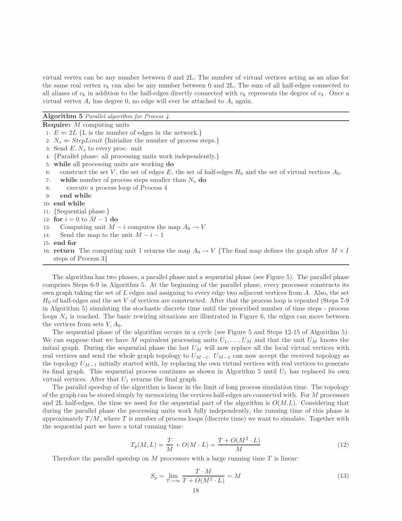
Algorithm 5 Parallel algorithm for Process 4.

Require: M computing units1: E ⇐ 2L L is the number of edges in the network.2: Ns ⇐ StepLimit Initialize the number of process steps.3: Send E, Ns to every proc. unit4: Parallel phase: all processing units work independently.5: while all processing units are working do

6: construct the set V , the set of edges E, the set of half-edges H0 and the set of virtual vertices A0.7: while number of process steps smaller than Ns do

8: execute a process loop of Process 49: end while

10: end while

11: Sequential phase.12: for i = 0 to M − 1 do

13: Computing unit M − i computes the map A0 → V14: Send the map to the unit M − i − 115: end for

16: return The computing unit 1 returns the map A0 → V The final map defines the graph after M × Isteps of Process 3

The algorithm has two phases, a parallel phase and a sequential phase (see Figure 5). The parallel phasecomprises Steps 6-9 in Algorithm 5. At the beginning of the parallel phase, every processor constructs itsown graph taking the set of L edges and assigning to every edge two adjacent vertices from A. Also, the setH0 of half-edges and the set V of vertices are constructed. After that the process loop is repeated (Steps 7-9in Algorithm 5) simulating the stochastic discrete time until the prescribed number of time steps - processloops Ns is reached. The basic rewiring situations are illustrated in Figure 6, the edges can move betweenthe vertices from sets V, A0.

The sequential phase of the algorithm occurs in a cycle (see Figure 5 and Steps 12-15 of Algorithm 5).We can suppose that we have M equivalent processing units U1, . . . , UM and that the unit UM knows theinitial graph. During the sequential phase the last UM will now replace all the local virtual vertices withreal vertices and send the whole graph topology to UM−1. UM−1 can now accept the received topology asthe topology UM−1 initially started with, by replacing the own virtual vertices with real vertices to generateits final graph. This sequential process continues as shown in Algorithm 5 until U1 has replaced its ownvirtual vertices. After that U1 returns the final graph.

The parallel speedup of the algorithm is linear in the limit of long process simulation time. The topologyof the graph can be stored simply by memorizing the vertices half-edges are connected with. For M processorsand 2L half-edges, the time we need for the sequential part of the algorithm is O(M.L). Considering thatduring the parallel phase the processing units work fully independently, the running time of this phase isapproximately T/M , where T is number of process loops (discrete time) we want to simulate. Together withthe sequential part we have a total running time:

Tp(M, L) =T

M+ O(M · L) =

T + O(M2 · L)

M(12)

Therefore the parallel speedup on M processors with a large running time T is linear:

Sp = limT→∞

T · M

T + O(M2 · L)= M (13)

18

0

20

40

60

80

100

120

140

160

180

200

1 2 3 4 5 6

#processes per 2 cores vs runtime in s

distributerewirecollect

Figure 7: (color online) The results of experiments showing the dependence between number of processes (x-axis) on onecore and the algorithm performance (y-axis). The performance is measured in seconds, and the time bars have three timecomponents: initialization time (distribute), the parallel phase time (rewire) and the collection time (collect). The process wassimulated for 5 ·108 steps on a network with 106 nodes and 4 ·106 edges. The optimal choice in our case is to allocate 1 processper core because hyperthreading does help only marginally in the case of core overloading with even number of processes.

This is also supported by the experiments where we show that in practical situations the influence of thesequential phase can be neglected. Moreover, the complexity of the sequential part of the algorithm can befurther improved by the observation that the order in which the maps are applied has no influence on theresult. Therefore, we can suppose that a tree organization of the map transition in a bottom-up fashion canintroduce a parallel logarithmic speed-up within this phase of the algorithm.

We can also think of a modified version of the parallel algorithm, where the processing units are simulatinga smaller chunk of process loops (time steps) and the sequential phases of the algorithm are interleaving theparallel phases. In this case the sequential map reconstruction process has to cycle several times throughall processors until the final discrete process time is reached. In this case, each processor has to restart theparallel phase with a new set of virtual vertices, once finished the intermediate mapping step. This versioncan be useful when each processor has to check or correct its own progress from time to time, or when weneed some intermediate results.

5. Experimental Results

To verify the parallel algorithm from the previous section we developed an experimental framework onthe HPC Cluster Brutus [6] located at ETH Zurich. Brutus is currently ranking 88 in the TOP500 [16]list of high-performance computers. The Brutus architecture consists of 10000 cores with several types ofAMD processors. The ranking was done on a homogeneous subsystem of Brutus consisting of 410 nodeswith four quad-core AMD Opteron 8380 CPUs and 32 GB of RAM (6560 cores). All nodes are connectedto the cluster’s Gigabit Ethernet backbone, 256 nodes use a high-speed Quadrics QsNetII network and 508nodes are connected to a high-speed InfiniBand QDR network. To program the parallel algorithm we usedMPI library [12].

The performance of the algorithm is measured in seconds. Every measurement consists of three timemeasures of Algorithm 5: the initialization time during which the initial graph is sent to all computing units

19

0

20

40

60

80

100

120

140

160

1 2 4 8 16 32 64 128

#cores vs runtime in s

distributerewirecollect

Figure 8: (color online) The figure illustrates a set of experiments for Algorithm 5 where the task is distributed on up to128 cores. The performance is measured in seconds, and the bars contain three time components: the initialization time(distribute), the parallel phase time (rewire) and the collection time (collect). The process was simulated for 5 · 108 steps ona network with 106 nodes and 4 · 106 edges. For fixed number of simulation steps, the sequential part of the algorithm mustprevail, if the number of cores increases over certain threshold.

(denoted with ”distribute”), time of parallel computation (”rewire”) and time of the sequential collectionphase (”collect”). To reduce the noise, we repeat the computation for every parameter set 10 times andaverage the results. The process is simulated for 5 · 108 steps on a network with 4 · 106 edges and 106 nodes.To consider the parallel speedup, we repeat the same simulation with 1,2,4,...,64 and 128 cores lying onnodes connected with InfiniBand QDR network. As we argued above, it is sufficient to store only half-edgesto represent the graph (the vertices with degree 0 does not need to be stored for our algorithm), thereforeto illustrate the scaling with respect to the graph size, we repeat the experiments with 2,4 and 8 times 106

edges. The sequential part of the algorithm (collect) is implemented using a bottom up tree data structurewhich has logarithmic time dependency on the number of processors.

The queue management system of Brutus cluster does not allow to have more processes resp. threads on1 core. However, we were principally interested whether a hyperthreading or other architectural aspects canbring a principal speedup for our particular type and implementation of the algorithm. Because the operatingsystem in our algorithm interprets the same sequence of instructions, we expected a neglectable effect. Thisfact is confirmed by our experiments, illustrated in Figure 7 which were computed on our developmentplatform where the computation was constrained to 2 cores - 1 processor. In this set of experiments wedistributed the task to the increasing number of processes (x-axis) to see how the speedup of the algorithmdepends on the number of parallel processes on one core. The results confirm that in our case it is optimalto distribute 1 Process per core. Marginally, it is interesting to observe the difference between the even andthe odd number of processes.

In Figures 8 and 9 we can observe that the parallel algorithm scales linearly over the cluster. For thegiven number of iteration (5 · 108) the peak performance is achieved with 64 processes allocating 1 processfor every core. After that the saturation phase occurs caused by the sequential part of algorithm. Thescaling with increasing size of the graph is also linear as was predicted in the algorithm analysis. This isvisible in Figure 9 where the speedup only differs in the saturation phase where the sequential part of thealgorithm prevails. During the parallel phase of Algorithm 5 the processors work independently from each

20

1

2

4

8

16

32

2 4 8 16 32 64 128

speedup, different number of edges

2mio edges4mio edges8mio edges

Figure 9: (color online) The overall speedup of Algorithm 5 is linear up to the point of saturation where the sequential partprevails. The algorithm also linearly scales with the size of the graph as is illustrated by three experiments with 2 · 106, 4 · 106

and 8 · 106 edges.

other. This can be observed in both Figures 8 and 9. The overall speedup does not change its characterduring the passage between different nodes which happens at multiples of 16 cores. This shows that if thetask is distributed across more computing nodes resp. processors there is no observable slow-down effectbecause of the network latency.

6. Conclusions

In our paper we analyzed a parallel simulation of scale-free networks. For a fundamental class of non-growing networks with linear preference function, we provide a highly parallel algorithm, which has twophases. The first phase is fully parallel and has speed-up M , where M is the number of processing units.The second phase is sequential, but independent on simulation time T , which is the main source of complexity.On the other hand, we theoretically analyzed dependencies which are prohibiting parallelism for an exactprocess. Our theoretical interest stems from the difficulties we observed when we tried to design a parallelalgorithm for simulation of general scale-free networks. The difficulties are arising from the fact that thepreferential selection step, which is used in most scale-free network models, is strongly dependent on thedegree distribution. This in turn changes with high probability during a stochastic equilibrium processwhich generates scale-free networks. This is valid for a wide range of nonlinear preference functions.

For many networks, the linear preference function can provide a sufficient approximation for the simula-tion of network evolution. However, an interesting future question, which we believe is solvable, is whetherone can approximate the nonlinear preference function with a piecewise linear function. To provide a parallelalgorithm in this case, it is necessary to consider at least two problems. First problem is how to handle thetransition from one linear function segment to another - we suppose that a method is needed how to pre-compute larger maps providing sufficient information to handle the transition to a different linear segment,and the second problem is to generalize the factorization in equation (11).

Another method to handle the preferential attachment consist in approximations of the process whichwould allow to neglect the effect of degree distribution changes. We suppose that such method is possiblefor wide class of networks but more research would be needed to know under which conditions and to which

21

extend such propagation can be neglected. Naturally, for many practical problems an empirical evidencecan be elaborated, how many process steps can be simulated before a global update of degree distributionis necessary.

Theoretically, it would be interesting to investigate larger classes of preference functions. In Theorem 6, adifferent method might be needed to estimate the probability for different classes of networks and preferencefunctions. The estimation method would also need improvement if we want to consider very sparse networkswhich have average degree near zero.

7. Acknowledgements

The authors would like to thank professor Peter Widmayer for inspiring discussions and ongoing supportof this project.

References

[1] R. Albert and A.-L. Barabasi. Statistical mechanics of complex networks. Rev. Modern Phys., 74:47–97, 2002.[2] D.A. Bader and K. Madduri. Snap, small-world network analysis and partitioning: An open-source parallel graph frame-

work for the exploration of large-scale networks. In Parallel and Distributed Processing, 2008. IPDPS 2008. IEEE

International Symposium on, pages 1–12, April 2008.[3] A.-L. Barabasi and R. Albert. Emergence of scaling in random networks. Science, 286(509), 1999.[4] A.-L. Barabasi, R. Albert, and H. Jeong. Mean-field theory for scale-free random networks. Physica A, (272), 1999.[5] S. Boccalettia, V. Latorab, Y. Morenod, M. Chavezf, and D.-U. Hwanga. Complex networks: Structure and dynamics.

Physics Reports, 424:175–308, 2006.[6] ETH Cluster Brutus. http://en.wikipedia.org/wiki/brutus cluster. Wikipedia on Brutus, the high performance cluster at

ETH Zurich, 2009.[7] A. Cami and N. Deo. Techniques for analyzing dynamic random graph models of web-like networks: An overview.

Networks, 51(4):211–255, 2008.[8] L. da Fontoura Costa, O. N. Oliveira Jr., G. Travieso, F. A. Rodrigues, P. R. V. Boas, M. P. Viana, L. Antiqueira, and

L. E. Correa da Rocha. Analyzing and modeling real-world phenomena with complex networks: A survey of applications.arXiv.org, (arXiv:0711.3199v3), 2008.

[9] G. D’Angelo and S. Ferretti. Simulation of scale-free networks. In Simutools ’09: Proceedings of the 2nd International

Conference on Simulation Tools and Techniques, pages 1–10, ICST, Brussels, Belgium, Belgium, 2009. ICST (Institutefor Computer Sciences, Social-Informatics and Telecommunications Engineering).

[10] S. N. Dorogovtsev and J. F. F. Mendes. Evolution of networks. Oxford University Press, 2003.[11] T. S. Evans and A. D. K. Plato. Exact solution for the time evolution of network rewiring models. Physical Review E,

75(056101), 2007.[12] MPI Forum. http://www.mpi-forum.org/. World Wide Web electronic publication of official MPI standards documents,

2009.[13] T. Hruz, M. Natora, and M. Agrawal. Higher-order distributions and nongrowing complex networks without multiple

connections. Physical Review E, 77(046101), 2008.[14] H. Jeong, B. Tombor, R. Albert, Z. N. Oltvai, and A.-L. Barabasi. The large-scale organization of metabolic networks.

Nature, 407:651–654, 2000.[15] K. Madduri and D. A. Bader. Compact graph representations and parallel connectivity algorithms for massive dynamic

network analysis. Parallel and Distributed Processing Symposium, International, 0:1–11, 2009.[16] H. Meuer, E. Strohmaier, J. Dongarra, and H. Simon. http://www.top500.org. World Wide Web electronic publication

of the Top 500 Supercomputer Sites, November 2009.[17] M. Mihail, C. Papadimitriou, and A. Saberi. On certain connectivity properties of the internet topology. Journal of

Computer and System Sciences, 72:239–251, 2006.[18] M. E. J. Newman. The structure and function of complex networks. Physical Review E, 45(2):167256, 2003.[19] Kwangho Park, Ying-Cheng Lai, and Nong Ye. Self-organized scale-free networks. Physical Review E, 72(026131), 2005.[20] A. Wagner and D. A. Fell. The small world inside large metabolic networks. Proc. R. Soc. Lond. B, 268:1803–1810, 2001.[21] D. J. Watts and S. H. Strogatz. Collective dynamics of small-world networks. Nature, 393:440–442, 1998.[22] A. Yoo and K. Henderson. Parallel generation of massive scale-free graphs. arxiv.org, (arXiv:1003.3684v1), 2010.[23] A. Youssef. A parallel algorithm for random walk construction with application to the monte carlo solution of partial

differential equations. IEEE Trans. Parallel Distrib. Syst., 4(3):355–360, 1993.

22