Embed Size (px)
Citation preview

PARALLEL IMPLEMENTATION OF DIJKSTRA'S ALGORITHM USING MPI
LIBRARY ON A CLUSTER.
INSTRUCUTOR: DR RUSS MILLER
ADITYA PORE

THE PROBLEM AT HAND
Given : A directed graph ,G = (V, E) . Cardinalities |V| = n, |E| = m.
S(Source ): distinguished vertex of the graph.
w : weight of each edge, typically, the distance between the two vertexes.
Single source shortest path: The single source shortest path (SSSP)
problem is that of computing, for a given source vertex s and a destination
vertex t, the weight of a path that obtains the minimum weight among all the
possible paths.

DIJKSTRA’s ALGORITHM AT A GLANCE
Dijkstra’s algorithm is a graph search algorithm that solves single-source shortest path for a graph with nonnegative weights.
Widely used in network routing protocol, e.g., Open Shortest PathFirst (OSPF) protocol
24 Node US-Mesh Network
How to reach Downtown from
Maple Road??
Dijkstra’s Algorithm
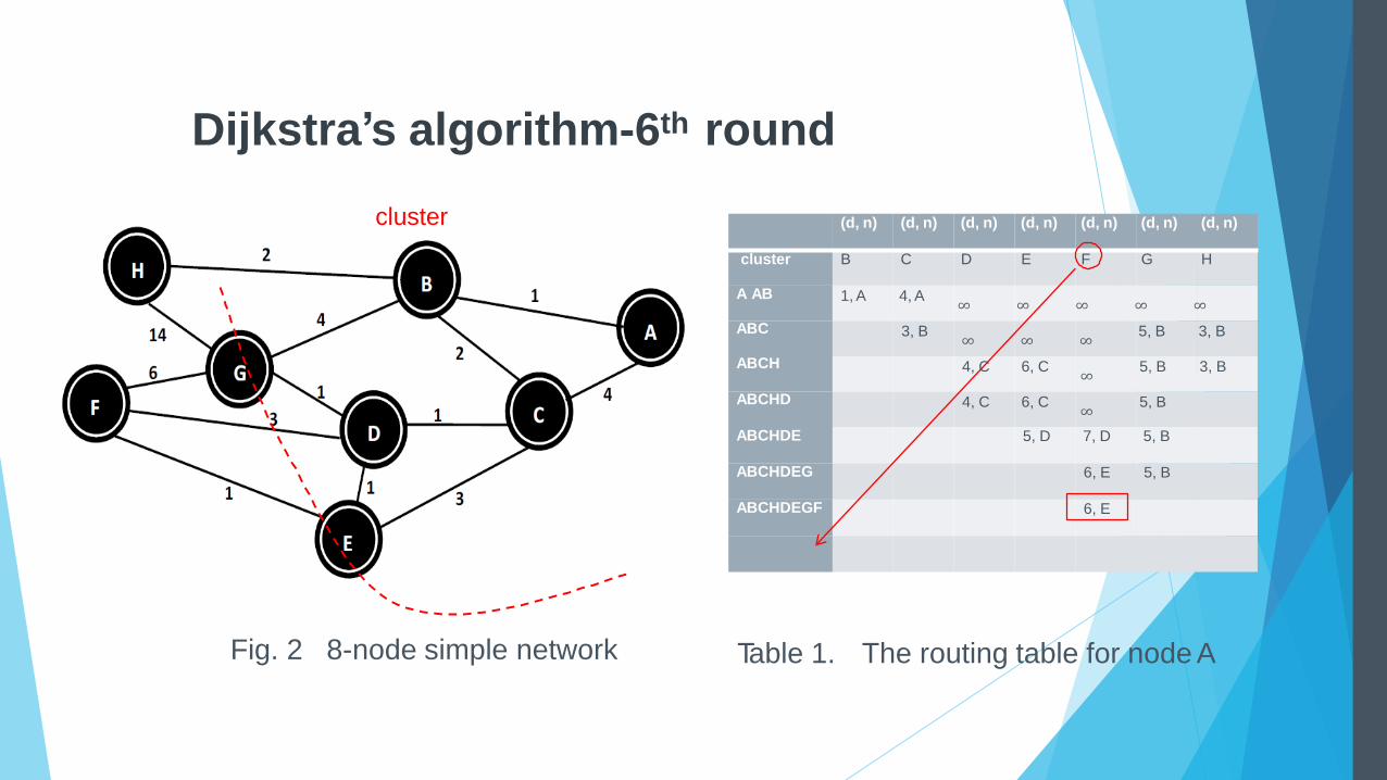
Fig. 2 8-node simple network Table 1. The routing table for node A
(d, n) (d, n) (d, n) (d, n) (d, n) (d, n) (d, n)
cluster
A AB
ABC
ABCH
ABCHD
ABCHDE
ABCHDEG
ABCHDEGF
B C D E F G H
1, A 4, A ∞ ∞ ∞ ∞ ∞
3, B ∞ ∞ ∞
5, B 3, B
4, C 6, C ∞
5, B 3, B
4, C 6, C ∞
5, B
5, D 7, D 5, B
6, E 5, B
6, E
LETS GET TO KNOW THE ALGORITHM WITH AN EXAMPLE

cluster
Dijkstra’s algorithm 1st round
Fig. 2 8-node simple network Table 1. The routing table for node A
(d, n) (d, n) (d, n) (d, n) (d, n) (d, n) (d, n)
cluster
A
AB
B C D E F G H
1, A 4, A ∞ ∞ ∞ ∞ ∞

Dijkstra’s algorithm-2nd round
cluster
Fig. 2 8-node simple network Table 1. The routing table for node A
(d, n) (d, n) (d, n) (d, n) (d, n) (d, n) (d, n)
cluster
A
AB
ABC
B C D E F G H
1, A 4, A ∞ ∞ ∞ ∞ ∞
3, B ∞ ∞ ∞ 5, B 3, B
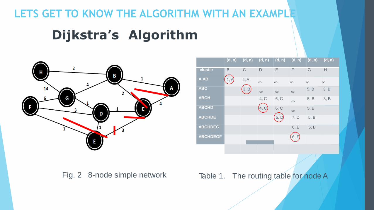
Dijkstra’s algorithm-3rd round
cluster
Fig. 2 8-node simple network Table 1. The routing table for node A
(d, n) (d, n) (d, n) (d, n) (d, n) (d, n) (d, n)
cluster
A AB
ABC
ABCH
B C D E F G H
1, A 4, A ∞ ∞ ∞ ∞ ∞
3, B ∞ ∞ ∞
5, B 3, B
4, C 6, C ∞ 5, B 3, B
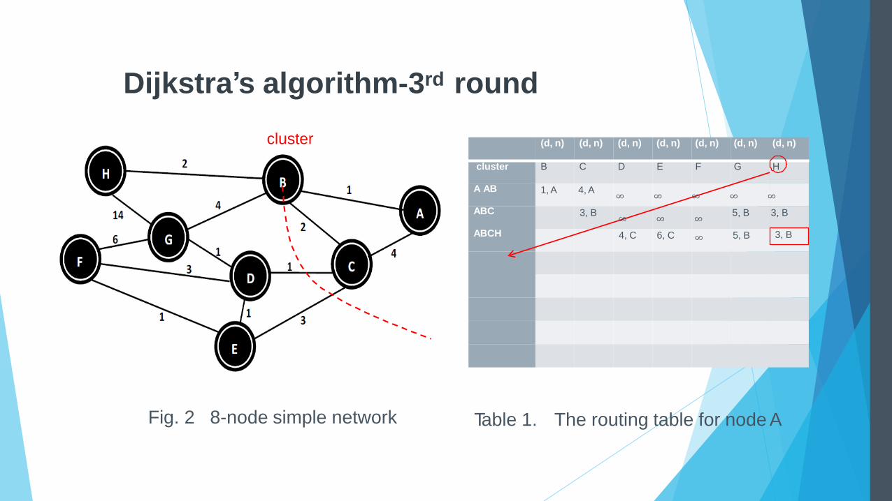
Dijkstra’s algorithm-4th round
cluster
Fig. 2 8-node simple network Table 1. The routing table for node A
(d, n) (d, n) (d, n) (d, n) (d, n) (d, n) (d, n)
cluster
A AB
ABC
ABCH
ABCHD
B C D E F G H
1, A 4, A ∞ ∞ ∞ ∞ ∞
3, B ∞ ∞ ∞
5, B 3, B
4, C 6, C ∞
5, B 3, B
4, C 6, C ∞ 5, B

Dijkstra’s algorithm-5th round
cluster
Fig. 2 8-node simple network Table 1. The routing table for node A
(d, n) (d, n) (d, n) (d, n) (d, n) (d, n) (d, n)
cluster
A AB
ABC
ABCH
ABCHD
ABCHDE
B C D E F G H
1, A 4, A ∞ ∞ ∞ ∞ ∞
3, B ∞ ∞ ∞
5, B 3, B
4, C 6, C ∞
5, B 3, B
4, C 6, C ∞
5, B
5, D 7, D 5, B

Dijkstra’s algorithm-6th round
cluster
Fig. 2 8-node simple network Table 1. The routing table for node A
(d, n) (d, n) (d, n) (d, n) (d, n) (d, n) (d, n)
cluster
A AB
ABC
ABCH
ABCHD
ABCHDE
ABCHDEG
B C D E F G H
1, A 4, A ∞ ∞ ∞ ∞ ∞
3, B ∞ ∞ ∞
5, B 3, B
4, C 6, C ∞
5, B 3, B
4, C 6, C ∞
5, B
5, D 7, D 5, B
6, E 5, B
6, E
Dijkstra’s algorithm-6th round
cluster
Fig. 2 8-node simple network Table 1. The routing table for node A
(d, n) (d, n) (d, n) (d, n) (d, n) (d, n) (d, n)
cluster
A AB
ABC
ABCH
ABCHD
ABCHDE
ABCHDEG
ABCHDEGF
B C D E F G H
1, A 4, A ∞ ∞ ∞ ∞ ∞
3, B ∞ ∞ ∞
5, B 3, B
4, C 6, C ∞
5, B 3, B
4, C 6, C ∞
5, B
5, D 7, D 5, B
6, E 5, B
6, E

SEQUENTIAL DIJKSTRA’S ALGORITHM
Create a cluster cl[V]
Given a source vertex s
While (there exist a vertex that is not in thecluster cl[V])
{
FOR (all the vertices outside the cluster)
Calculate the distance from non-
member vertex to s through the clusterEND
** O(V) **
Select the vertex with the shortest path and
add it to the cluster** O(V) **
}
ANALOGY

DIJKSTRA’S ALGORITHM
Running time O(V )
In order to obtain the routing table, we need O(V) roundsiterations (until all the vertices are included in the cluster).
In each round, we will update the value for O(V) vertices andselect the closest vertex, so the running time in each roundis O(V).
So, the total running time is O(V )
Disadvantages:
If the scale of the network is too large, then it will cost along time to obtain the result.
For some time-sensitive app or real-time services, we needto reduce the running time.
2
2
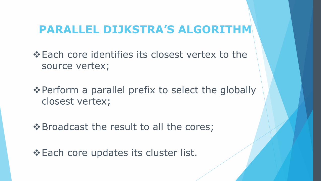
PARALLEL DIJKSTRA’S ALGORITHM
Each core identifies its closest vertex to the source vertex;
Perform a parallel prefix to select the globally closest vertex;
Broadcast the result to all the cores;
Each core updates its cluster list.

Parallel Dijkstra’s
Step 1: findthe closestnode in mysubgroup.
algorithm
Step 2: use
parallel prefix to find the global closest.
(d, n) (d, n) (d, n) (d, n) (d, n) (d, n) (d, n)
cluster
A AB
ABC
ABCH
ABCHD
ABCHDE
ABCHDEG
ABCHDEGF
B C D E F G H
1, A 4, A ∞ ∞ ∞ ∞ ∞
3, B ∞ ∞ ∞
5, B 3, B
4, C 6, C ∞
5, B 3, B
4, C 6, C ∞
5, B
5, D 7, D 5, B
6, E 5, B
6, E
THE ACTUAL ALGORITHM AT WORK
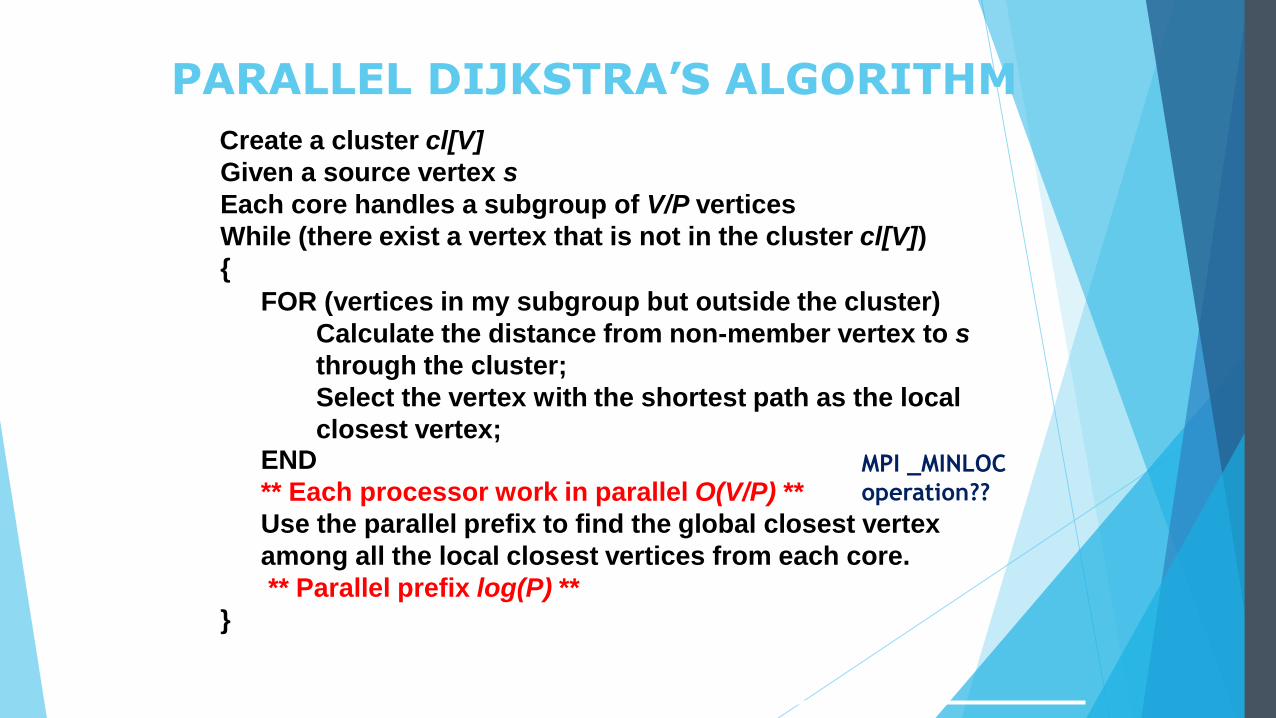
PARALLEL DIJKSTRA’S ALGORITHM
Create a cluster cl[V]
Given a source vertex s
Each core handles a subgroup of V/P vertices
While (there exist a vertex that is not in the cluster cl[V])
{
FOR (vertices in my subgroup but outside the cluster)
Calculate the distance from non-member vertex to s
through the cluster;
Select the vertex with the shortest path as the local
closest vertex;END
** Each processor work in parallel O(V/P) **
Use the parallel prefix to find the global closest vertex
among all the local closest vertices from each core.
** Parallel prefix log(P) **
}
MPI _MINLOC
operation??

PARALLEL DIJKSTRA’S ALGORITHM
2
.
RUNNING TIME : O(V /P +V log(P))
P is the number of cores used.
In order to obtain the routing table, we need O(V) rounds iteration (until all the
vertices are included in the cluster).
In each round, we will update the value for O(V) vertices using P cores running
independently, and use the parallel prefix to select the global closest vertex, so
the running time in each round is O(V/P)+O(log(P)).
So, the total running time is O(V /P +V log(P))2
2

RESULTS AND ANALYSIS
Implemented using MPI : Stats Averaged over 10 rounds of Computation.
Establish trade-off between running times as a function of number of cores
deployed.
Evaluate speed up and efficiency!!!!
EXPERIMENT A: (More Graphs and Analysis)
Compute for fixed size input:10000
Run Routines for :1 32-core node,3 12-core node,16 dual-core
EXPERIMENT B: (Achieved Desired Results)
Compute for different input size: Typically 625,2500,10000
Run Routine on 1 32-core Node.

EXPERIMENT A : RUN TIME
Number of
Cores
1 2 4 8 16 32
Configurations RUNTIMES I N SECONDS
1)16*2 Core 4.37263 2.36273 1.98442 5.48834 7.89371 12.65342
2)3*12 Core 4.67321 2.42865 1.34567 0.72341 2.88764 6.45321
3)1*32 Core 5.45321 2.68753 1.56782 0.86754 0.89654 1.23609
Tabulation of Results :
Relationship Observed : Number of Cores Versus The Running Time(seconds)
Conclusions:
(a) Run Time is Inversely proportional to number of cores :Cores belong to the
same node in cluster
(b) Significant Increase observed for two configurations out of three, namely
16*2 Core and 3*12 Core.

EXPERIMENT A : RUN TIME GRAPHICAL DESCRIPTION OF RUN TIME ANALYSIS
0
2
4
6
8
10
12
14
1 2 4 8 16 32
Run-Time(Seconds) vs Number of Cores
16*2 Core 3*12 Core 1*32 Core

EXPERIMENT A : SPEED UP
Tabulation of Results :
Relationship Observed : Number of Cores Versus The Speed-Up
Conclusions:
(a) Speed-Up is Directly proportional to number of cores :Cores belong to the
same node in cluster
(b) Significant Decrease observed for two configurations out of three, namely
16*2 Core and 3*12 Core.
Number of
Cores
1 2 4 8 16 32
Configurations SPEED UP: GIVES A MEASURE OF SCALABILITY OF THE SYSTEM
16*2 Core 1 1.85324 2.10978 0.85432 0.54332 0.32456
3*12 Core 1 1.94433 3.75567 6.74352 1.86432 0.86032
1*32 Core 1 1.98765 3.66541 6.40321 6.78432 4.89543

EXPERIMENT A : SPEED-UPGRAPHICAL DESCRIPTION OF SPEED-UP ANALYSIS
1
1.853242.10978
0.854320.54332 0.32456
1
1.94433
3.75567
6.74352
1.86432
0.860321
1.98765
3.66541
6.40321
6.78432
4.89543
0
1
2
3
4
5
6
7
8
1 2 4 8 16 32
NUMBER OF CORES VS SPEED-UP
16*2 Core 3*12 Core 1*32 Core
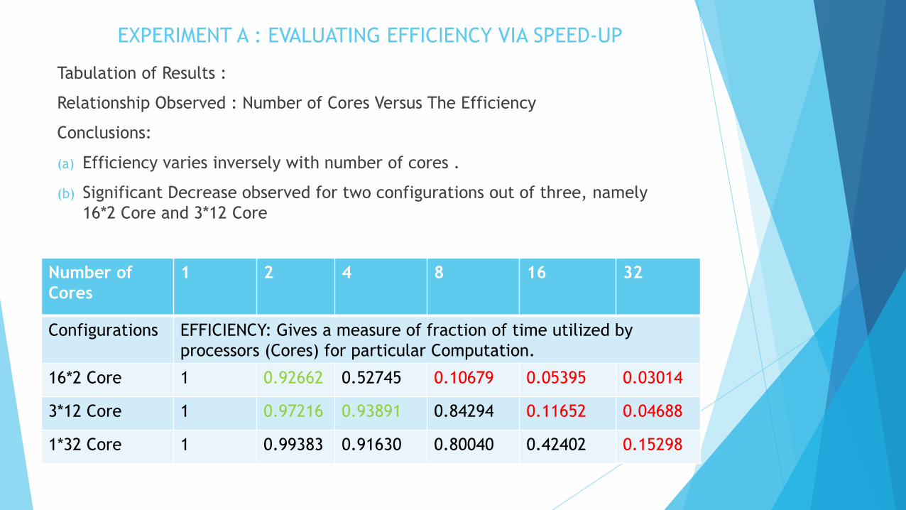
EXPERIMENT A : EVALUATING EFFICIENCY VIA SPEED-UP
Tabulation of Results :
Relationship Observed : Number of Cores Versus The Efficiency
Conclusions:
(a) Efficiency varies inversely with number of cores .
(b) Significant Decrease observed for two configurations out of three, namely
16*2 Core and 3*12 Core
Number of
Cores
1 2 4 8 16 32
Configurations EFFICIENCY: Gives a measure of fraction of time utilized by
processors (Cores) for particular Computation.
16*2 Core 1 0.92662 0.52745 0.10679 0.05395 0.03014
3*12 Core 1 0.97216 0.93891 0.84294 0.11652 0.04688
1*32 Core 1 0.99383 0.91630 0.80040 0.42402 0.15298

EXPERIMENT A : EFFICIENCYGRAPHICAL DESCRIPTION OF ANALYSIS
100
92
52
10 5 3
10097
93
84
11 4
100 99
91
80
42
15
0
20
40
60
80
100
120
1 2 4 8 16 32
NUMBER OF CORES VS EFFICIENCY(%)
16*2 Core 3*12 Core 1*32 Core

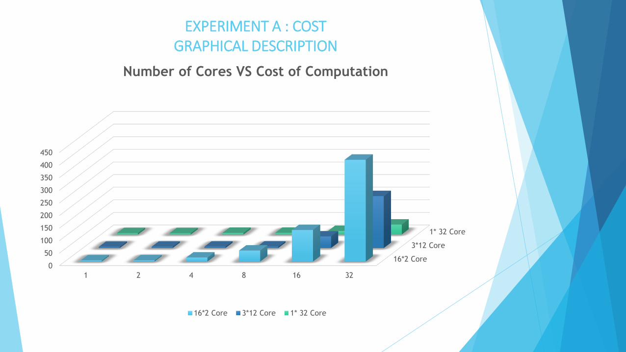
EXPERIMENT A : COST
Tabulation of Results :
Relationship Observed : Number of Cores Versus Cost of Computation
Conclusions:
(a) Run Time is Inversely proportional to number of cores
(b) Significant Increase observed for 16*2 Core configuration.
(c) Parallel computing is cost effective for modest speedups.
Number of
Cores
1 2 4 8 16 32
Configurations Cost: Product of number of cores(resources) used times execution time
16*2 Core 4.37263 4.72546 15.93768 43.90672 126.29936 404.9094
3*12 Core 4.67321 4.85730 5.38268 5.78728 46.20224 206.5027
1*32 Core 5.45321 5.37506 6.27128 6.94032 14.34464 39.55488
EXPERIMENT A : COSTGRAPHICAL DESCRIPTION
16*2 Core
3*12 Core
1* 32 Core
0
50
100
150
200
250
300
350
400
450
1 2 4 8 16 32
Number of Cores VS Cost of Computation
16*2 Core 3*12 Core 1* 32 Core

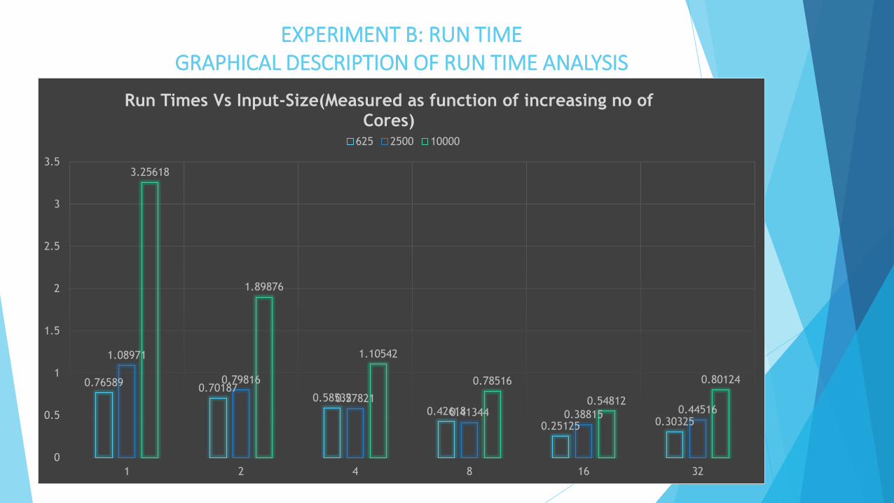
EXPERIMENT B : RUN TIME
Tabulation of Results :
Relationship Observed : Input-Size VS Running-Time
Conclusions:
(a) Run Time varies Inversely with the number of Cores.
(b) Algorithm found to be most-effective performance-wise for 16 Core configuration.
(c) 32-Cores: Run time increases Slightly as communication overhead defeats the purpose of
using more number of cores for computation.
Number of
Cores
1 2 4 8 16 32
Input-Size RUNTIME IN SECONDS
625 0.76589 0.70187 0.58532 0.42618 0.25125 0.30325
2500 1.08971 0.79816 0.57821 0.41344 0.38815 0.44516
10000 3.25618 1.89876 1.10542 0.78516 0.54812 0.80124
EXPERIMENT B: RUN TIME GRAPHICAL DESCRIPTION OF RUN TIME ANALYSIS
0.765890.70187
0.58532
0.42618
0.25125 0.30325
1.08971
0.79816
0.57821
0.41344 0.38815 0.44516
3.25618
1.89876
1.10542
0.78516
0.54812
0.80124
0
0.5
1
1.5
2
2.5
3
3.5
1 2 4 8 16 32
Run Times Vs Input-Size(Measured as function of increasing no of Cores)
625 2500 10000
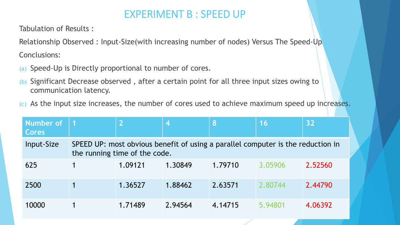
EXPERIMENT B : SPEED UPTabulation of Results :
Relationship Observed : Input-Size(with increasing number of nodes) Versus The Speed-Up
Conclusions:
(a) Speed-Up is Directly proportional to number of cores.
(b) Significant Decrease observed , after a certain point for all three input sizes owing to
communication latency.
(c) As the input size increases, the number of cores used to achieve maximum speed up increases.
Number of
Cores
1 2 4 8 16 32
Input-Size SPEED UP: most obvious benefit of using a parallel computer is the reduction in
the running time of the code.
625 1 1.09121 1.30849 1.79710 3.05906 2.52560
2500 1 1.36527 1.88462 2.63571 2.80744 2.44790
10000 1 1.71489 2.94564 4.14715 5.94801 4.06392

EXPERIMENT B : SPEED-UPGRAPHICAL DESCRIPTION OF SPEED-UP ANALYSIS
625
2500
10000
1 2 4 8 16 32
1 1.091211.30849
1.7971
3.05906
2.5256
11.36527
1.88462
2.635712.80744
2.4479
1
1.71489
2.94564
4.14715
5.94801
4.06392
INPUT-SIZE(INCREASING NUMBER OF NODES)VS SPEED-UP
625 2500 10000

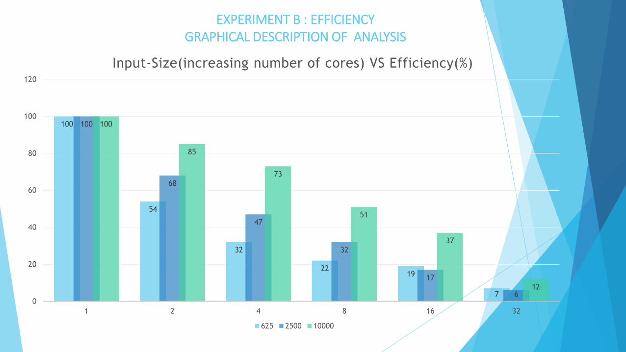
EXPERIMENT B : EVALUATING EFFICIENCY VIA SPEED-UP
Tabulation of Results :
Relationship Observed : Input-Size(Increasing number of cores )Versus The Efficiency
Conclusions:
(a) Efficiency varies inversely with number of cores .
(b) Significant Decrease observed as number of cores increases
(c) Gives an indication that benefit of reduced running time cannot outperform cost of operation.
Number of
Cores
1 2 4 8 16 32
Input-Size Efficiency: For example, if E = 50%, the processors are being used half of the
time to perform the actual computation
625 1 0.54560 0.32712 0.22463 0.19119 0.07893
2500 1 0.68263 0.47115 0.32946 0.17546 0.07649
10000 1 0.85744 0.73641 0.51834 0.37175 0.12699
EXPERIMENT B : EFFICIENCYGRAPHICAL DESCRIPTION OF ANALYSIS
100
54
32
2219
7
100
68
47
32
17
6
100
85
73
51
37
12
0
20
40
60
80
100
120
1 2 4 8 16 32
Input-Size(increasing number of cores) VS Efficiency(%)
625 2500 10000

A QUICK LOOK UP AT THE AMDAHL’S LAW
The maximum speed up that can be achieved by using N resources is :
1/(F+(1-F)/N).
As an example, if F is only 10%, the problem can be sped up by only a
maximum of a factor of 10, no matter how large the value of N used.
A great part of the craft of parallel programming consists of
attempting to reduce F to the smallest possible value.
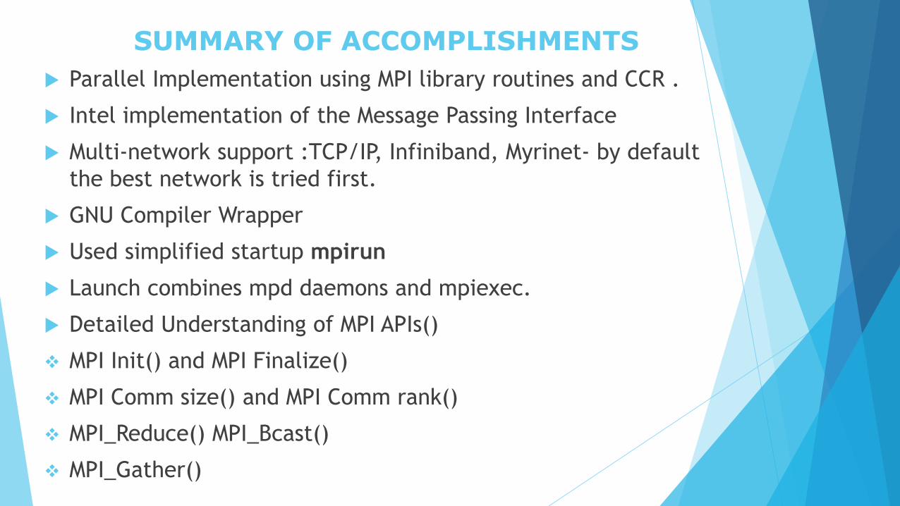
SUMMARY OF ACCOMPLISHMENTS
Parallel Implementation using MPI library routines and CCR .
Intel implementation of the Message Passing Interface
Multi-network support :TCP/IP, Infiniband, Myrinet- by default
the best network is tried first.
GNU Compiler Wrapper
Used simplified startup mpirun
Launch combines mpd daemons and mpiexec.
Detailed Understanding of MPI APIs()
MPI Init() and MPI Finalize()
MPI Comm size() and MPI Comm rank()
MPI_Reduce() MPI_Bcast()
MPI_Gather()
REFERENCES
Dijkstra, E. W. (1959). "A note on two problems in connection with graphs,". Numerische Mathematik 1: 269–271. doi:10.1007/BF01386390.
Cormen, Thomas H.; Leiserson, Charles E.; Rivest, Ronald L.; Stein, Clifford (2001). "Section 24.3: Dijkstra's algorithm". Introduction to Algorithms (Second ed.). MIT Press and McGraw-Hill. pp. 595–601. ISBN 0-262-03293-7.
A. Crauser, K. Mehlhorn, U. Meyer, P. Sanders, “A parallelization of Dijkstra’sshortest path algorithm”, in Proc. of MFCS’98, pp. 722-731, 1998.
Y. Tang, Y. Zhang, H. Chen, “A Parallel Shortest Path Algorithm Based on Graph-Partitioning and Iterative Correcting”, in Proc. of IEEE HPCC’08, pp. 155-161, 2008.
Stefano, A. Petricola, C. Zaroliagis, “On the implementation of parallel shortest path algorithms on a supercomputer”, in Proc. of ISPA’06, pp. 406-417, 2006.
http://www.cse.buffalo.edu/faculty/miller/Courses/CSE633/Ye-Fall-2012-CSE633.pdf

THANK-YOU
ANY QUESTIONS??