Parallel implementation of BLAS: general techniques for Level 3 BLAS

CONCURRENCY: PRACTICE AND EXPERIENCE, VOL. 9(9), 837–857 (SEPTEMBER 1997)

Parallel implementation of BLAS:general techniques for Level 3 BLASALMADENA CHTCHELKANOVA, JOHN GUNNELS, GREG MORROW, JAMES OVERFELT

AND ROBERT A. VAN DE GEIJN

The University of Texas at Austin, College of Natural Sciences, Department of Computer Sciences, Taylor Hall2124, Austin, Texas 78712-1188, USA

SUMMARYIn this paper, we present straightforward techniques for a highly efficient, scalable implementa-tion of common matrix–matrix operations generally known as the Level 3 Basic Linear AlgebraSubprograms (BLAS). This work builds on our recent discovery of a parallel matrix–matrixmultiplication implementation, which has yielded superior performance, and requires littlework space. We show that the techniques used for the matrix–matrix multiplication naturallyextend to all important Level 3 BLAS and thus this approach becomes an enabling technologyfor efficient parallel implementation of these routines and libraries that use BLAS. Representa-tive performance results on the Intel Paragon system are given. 1997 by John Wiley & Sons,Ltd.

1. INTRODUCTION

Over the last five years, we have learned a lot about how to parallelize dense linear algebralibraries[1–8]. Since much effort went into implementation of individual algorithms, itbecame clear that in order to parallelize entire sequential libraries, better approaches hadto be found. Perhaps the most successful sequential library, LAPACK[9,10], is built upona few compute kernels, known as the Basic Linear Algebra Subprograms (BLAS). Theseinclude the Level 1 BLAS (vector–vector operations)[11], Level 2 BLAS (matrix–vectoroperations)[12], and Level 3 BLAS (matrix–matrix operations)[13]. It is thus natural to tryto push most of the effort into parallelizing these kernels, in the hope that good parallelimplementations of codes that utilize these kernels will follow automatically. The aboveobservations lead to two related problems: first, how to specify the parallel BLAS andsecond, how to implement them. The former is left to those working to standardize parallelBLAS interfaces[14]. This paper concentrates on the latter issue.

Notice that the dense linear algebra community has always depended on fast implemen-tations of the BLAS provided by the vendors. Unless simple implementation techniques aredeveloped, construction and maintenance of the parallel BLAS becomes too cumbersome,making it much more difficult to convince the vendors to provide fast implementations.We therefore must develop fast reference implementations, so that the vendors need onlyperform minor optimizations.

In a recent paper[15], we describe a highly efficient implementation of matrix–matrixmultiplication, Scalable Universal Matrix Multiplication Algorithm (SUMMA), that hasmany benefits over alternative implementations[16–18]. These benefits include better per-formance, simpler and more flexible implementation, and a lower workspace requirement.In this paper, we show how the simple techniques developed in that paper can be extendedto all the Level 3 BLAS. The techniques are quite similar to those used to develop high

CCC 1040–3108/97/090837–21 $17.50 Received 31 October 19951997 by John Wiley & Sons, Ltd. Revised 23 May 1996

838 A. CHTCHELKANOVA ET AL.

performance sequential implementations of the Level 3 BLAS when only a fast matrix-multiplication is available[19].

2. NOTATION AND ASSUMPTIONS

2.1. Model of computation

We assume that the nodes of the parallel computer form an r × c mesh. While for theanalysis this is a physical mesh, the developed codes require only that the nodes can belogically configured as an r × c mesh. The p = rc nodes are indexed by their row andcolumn index and the (i, j) node will be denoted by Pij .

In the absence of network conflicts, communicating a message between two nodesrequires time α+ nβ, which is reasonable on machines like the Intel Paragon system[20].Parameters α and β represent the startup and cost per item transfer time, respectively.Performing a floating point computation requires time γ.

2.2. Data decomposition

We will assume the classical data decomposition, generally referred to as a two-dimensionalblock-wrapped, or block-cyclic, matrix decomposition[5].

In general, we would need to consider the case of matrices as being distributed using atemplate matrix as follows. Let template matrix X be partitioned as

X =

X00 X01 X02 · · ·X10 X11 X12 · · ·X20 X21 X22 · · ·

......

...

where Xij is an nr × nc submatrix. We will assume that the template is distributed tonodes so that Xij is assigned to node Pimod r,j mod c. In other words, the template is block-wrapped onto the (logical) two-dimensional mesh of nodes. The template matrix can bethought of as having infinite dimension. Since it does not really exist, it requires no space.For our implementations, the submatrices are square, i.e. nr = nc = nb, which we will callthe blocking factor. However, the techniques discussed in this paper encompass the moregeneral case.

Matrices A, B and C, involved in the matrix–matrix operation, are aligned to thistemplate by specifying the element of template X with which the upper-left-hand elementof the matrix is aligned, after which the elements of the matrices are distributed likecorresponding elements of the template.

2.3. Calling sequences

In this Section we show how sequential calling sequences can be easily generalized to par-allel calling sequences using the above observations. This is not because we are proposinga standard. We are merely trying to illustrate what kind of additional information must bespecified. We will illustrate this for the simplest case of the matrix–matrix multiplicationalgorithm only, under the assumption that it will be clear how this generalizes.

PARALLEL IMPLEMENTATION OF BLAS 839

The sequential calling sequence for the Level 3 BLAS Double precision GEneral Matrix-matrix Multiplication is

DGEMM ( "N", "N", M, N, K, ALPHA, A, LDA, B, LDB, BETA, C, LDC )

and C = αAB + βC.Here "N", "N" indicate that neither matrix A nor B are transposed, respectively. M and

N are the row and column dimensions of matrix C, and K is the ‘other’ dimension, in thiscase the column dimension of A and row dimension of B. Matrices A, B and C are storedin arrays A, B and C, respectively, which have leading dimensions LDA, LDB and LDC.

In distributing the matrices, it suffices to specify the following for each:

• the local array in which it is stored on this node. We will assume that we simply useA, B and C

• the local leading dimensions LLDA, LLDB and LLDC

• the blocking factor nb in parameter NB• MPI communicators indicating the row and column of the logical mesh: comm row

and comm col, and• the element of matrix template X with which the upper-right-hand element of the

matrices are aligned: the row, column pairs (IA, JA), (IB, JB) and (IC, JC),respectively.

Thus the calling sequence becomes

sB_DGEMM ( "N", "N", M, N, K, ALPHA, A, LLDA, IA, JA, B, LLDB, IB,

JB, BETA, C, LLDC, IC, JC )}

and C = αAB + βC.It will be assumed that NB is initialized through some initialization routine, as are

the parameters and assignment of the logical r × c mesh of nodes as part of the MPIcommunicators.

2.4. Simplifying assumptions

In our explanations, we assume for simplicity that

• α = 1 and β = 0• nr = nc = nb• m = n = k = Nnb, and• IA = JA = IB = JB = IC = JC = 1, i.e. the matrices are aligned with the

upper-left element of the template.

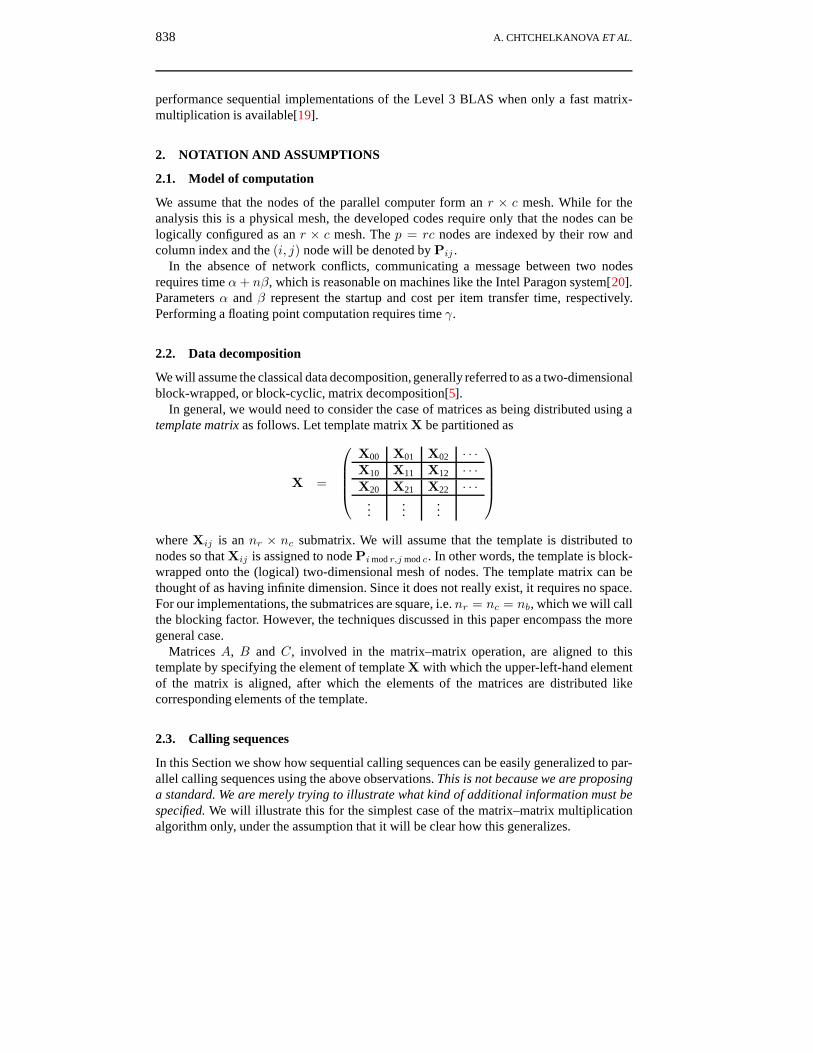
Thus, we will use the partitioning of the matrices

Y =

Y00 Y01 · · · Y0(N−1)

Y10 Y11 · · · Y1(N−1)

......

...Y(N−1)0 Y(N−1)1 · · · Y(N−1)(N−1)

(1)

with Y ∈ {A,B,C} and Yij of size nb × nb assigned to Pimod r,j mod c. (We realizethat slight confusion will result of our mixing of the Fortran convention of starting the


indexing of arrays with 1 and the indexing of the blocks starting at 0, which leads tosimpler explanations.)

3. PARALLEL ALGORITHMS FOR THE LEVEL 3 BLAS

In this Section, we give high level descriptions of the parallel implementations of all theLevel 3 BLAS.

3.1. Matrix-Matrix Multiplication (xGEMM)

3.1.1. Forming C = AB

In [15], we note the following:

C = AB =

A00

A10...

A(N−1)0

(

B00 B01 · · · B0(N−1)

)(2)

+

A01

A11...

A(N−1)1

(

B10 B11 · · · B1(N−1)

)+ · · · (3)

+

A0(N−1)

A1(N−1)

...A(N−1)(N−1)

(B(N−1)0 B(N−1)1 · · · B(N−1)(N−1)

) (4)

where A∗j (Bi∗) consists of nb columns (rows) and will be referred to as a column (row)panel.

In other words, the matrix–matrix multiplication can be implemented as a sequence ofN rank-nb updates.

The parallel implementation can now proceed as given in Figure 1.

in parallel C = 0for i = 0, N − 1

broadcast A∗i within rowsbroadcast Bi∗ within columnsin parallel

C = C +

A0i

A1i...

A(N−1)i

(Bi0 Bi1 · · · Bi(N−1)

)endfor

Figure 1. Pseudo-code for C = AB


It has been pointed out to us that this implementation has already been reported in [34].In that paper the benefits of overlapping communication and computation are also studied.

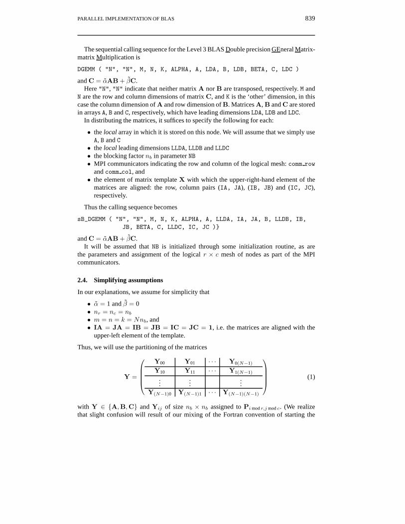
3.1.2. Forming C = ABT

One approach to implementing this case is to transpose matrix B followed by the algorithmpresented in the previous Section. In [15], we show how to avoid this initial communication:

C0i

C1i...

C(N−1)i

= A(

Bi0 Bi1 · · · Bi(N−1)

)

C can thus be computed a column panel at a time.The parallel implementation can now proceed as given in Figure 2.


broadcast BTi∗ within columnscompute C∗i = ABTi∗ by

computing local contributionsumming local contributions to column of nodesthat own C∗i

endfor

Figure 2. Pseudo-code for C = ABT

3.1.3. Forming C = ATB

This case can be implemented much like C = ABT.

3.1.4. Forming C = ATBT

On the surface, it appears that this case can be implemented much like C = AB bycommunicating row panels of A and column panels of B. However, this would computeCT, requiring a transpose operation to bring the data to the final destination. We nextdescribe a technique that transposes both matrix A and B, but only a row and column panelat a time. The benefit of this is that no work array is needed to store the transposed copy ofthe result matrix. We will limit ourselves considerably by only describing the algorithm forthe case where the mesh of nodes is square. How to generalize this approach will be brieflyindicated in the conclusion and in [22].


Note that

C = ATBT =

(A00 A01 · · · A0(N−1)

)T B00

B10...

B(N−1)0

T

(5)

+

(A10 A11 · · · A1(N−1)

)T

B01

B11...

B(N−1)1

T

+ · · · (6)

+ (A(N−1)0 A(N−1)1 · · · A(N−1)(N−1)

)T

B0(N−1)

B1(N−1)

...B(N−1)(N−1)

T

(7)

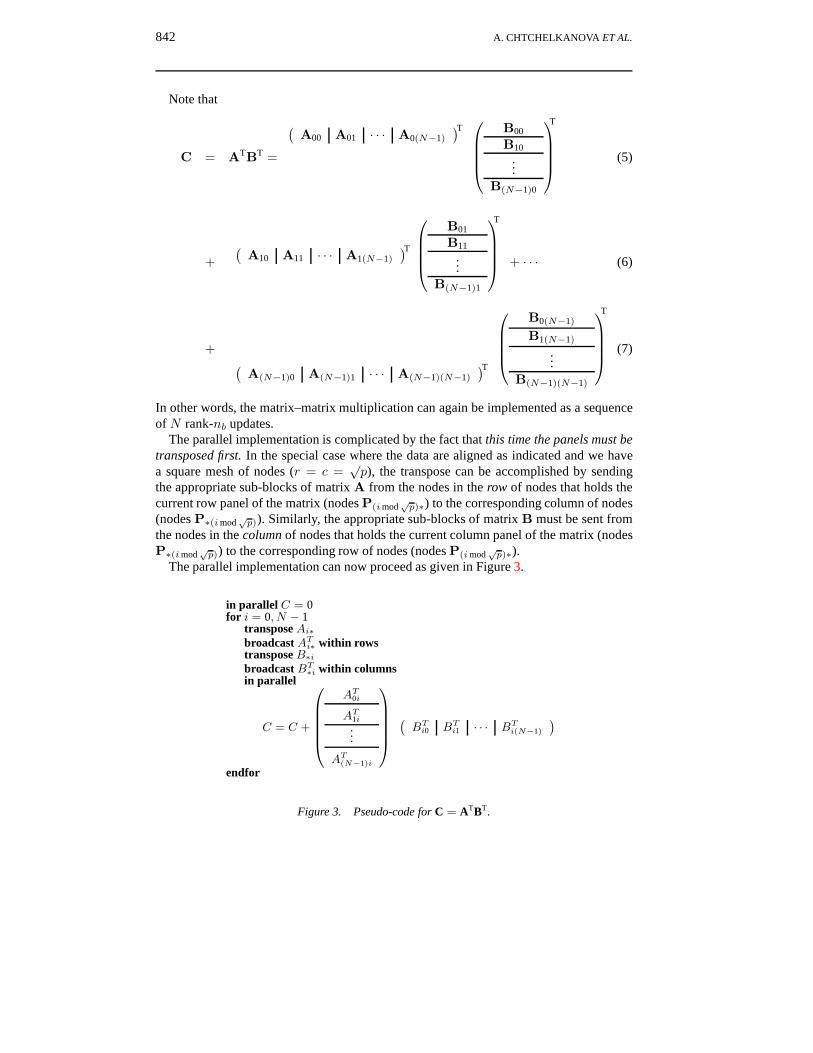
In other words, the matrix–matrix multiplication can again be implemented as a sequenceof N rank-nb updates.

The parallel implementation is complicated by the fact that this time the panels must betransposed first. In the special case where the data are aligned as indicated and we havea square mesh of nodes (r = c =

√p), the transpose can be accomplished by sending

the appropriate sub-blocks of matrix A from the nodes in the row of nodes that holds thecurrent row panel of the matrix (nodes P(imod

√p)∗) to the corresponding column of nodes

(nodes P∗(imod√p)). Similarly, the appropriate sub-blocks of matrix B must be sent from

the nodes in the column of nodes that holds the current column panel of the matrix (nodesP∗(imod

√p)) to the corresponding row of nodes (nodes P(imod

√p)∗).

The parallel implementation can now proceed as given in Figure 3.


transpose Ai∗broadcast ATi∗ within rowstranspose B∗ibroadcast BT∗i within columnsin parallel

C = C +

AT0i

AT1i...

AT(N−1)i

(BTi0 BTi1 · · · BTi(N−1)

)endfor

Figure 3. Pseudo-code for C = ATBT.


3.2. Triangular Matrix–Matrix Multiplication (xTRMM)

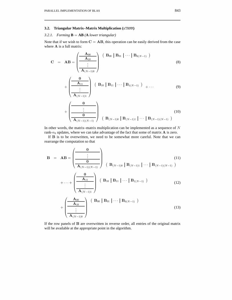
3.2.1. Forming B = AB (A lower triangular)

Note that if we wish to form C = AB, this operation can be easily derived from the casewhere A is a full matrix:

C = AB =

A00

A10...

A(N−1)0

(

B00 B01 · · · B0(N−1)

)(8)

+

0

A11...

A(N−1)1

(

B10 B11 · · · B1(N−1)

)+ · · · (9)

+

0...0

A(N−1)(N−1)

(B(N−1)0 B(N−1)1 · · · B(N−1)(N−1)

) (10)

In other words, the matrix–matrix multiplication can be implemented as a sequence of Nrank-nb updates, where we can take advantage of the fact that some of matrix A is zero.

If B is to be overwritten, we need to be somewhat more careful. Note that we canrearrange the computation so that

B = AB =

0...0

A(N−1)(N−1)

(B(N−1)0 B(N−1)1 · · · B(N−1)(N−1)

)(11)

+ · · ·+

0

A11...

A(N−1)1

(

B10 B11 · · · B1(N−1)

)(12)

+

A00

A10...

A(N−1)0

(

B00 B01 · · · B0(N−1)

)(13)

If the row panels of B are overwritten in reverse order, all entries of the original matrixwill be available at the appropriate point in the algorithm.


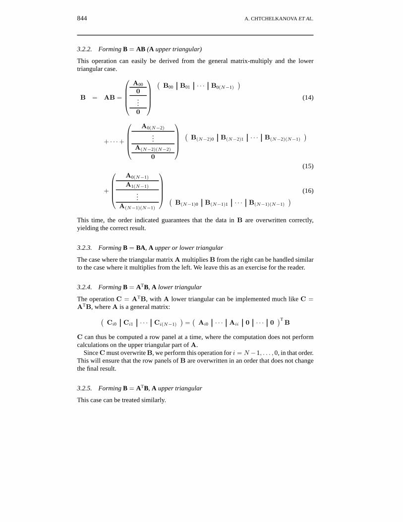
3.2.2. Forming B = AB (A upper triangular)

This operation can easily be derived from the general matrix-multiply and the lowertriangular case.

B = AB =

A00

0...0

(

B00 B01 · · · B0(N−1)

)(14)

+ · · ·+

A0(N−2)

...A(N−2)(N−2)

0

(

B(N−2)0 B(N−2)1 · · · B(N−2)(N−1)

)

(15)

+

A0(N−1)

A1(N−1)

...A(N−1)(N−1)

(B(N−1)0 B(N−1)1 · · · B(N−1)(N−1)

) (16)

This time, the order indicated guarantees that the data in B are overwritten correctly,yielding the correct result.

3.2.3. Forming B = BA, A upper or lower triangular

The case where the triangular matrix A multiplies B from the right can be handled similarto the case where it multiplies from the left. We leave this as an exercise for the reader.

3.2.4. Forming B = ATB, A lower triangular

The operation C = ATB, with A lower triangular can be implemented much like C =ATB, where A is a general matrix:(

Ci0 Ci1 · · · Ci(N−1)

)=(

Ai0 · · · Aii 0 · · · 0)T

B

C can thus be computed a row panel at a time, where the computation does not performcalculations on the upper triangular part of A.

Since C must overwrite B, we perform this operation for i = N−1, . . . , 0, in that order.This will ensure that the row panels of B are overwritten in an order that does not changethe final result.

3.2.5. Forming B = ATB, A upper triangular

This case can be treated similarly.


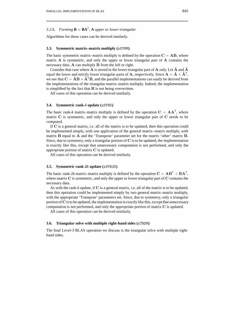
3.2.6. Forming B = BAT, A upper or lower triangular

Algorithms for these cases can be derived similarly.

3.3. Symmetric matrix–matrix multiply (xSYMM)

The basic symmetric matrix–matrix multiply is defined by the operation C = AB, wherematrix A is symmetric, and only the upper or lower triangular part of A contains thenecessary data. A can multiply B from the left or right.

Consider that case where A is stored in the lower triangular part of A only. Let A and Aequal the lower and strictly lower triangular parts of A, respectively. Since A = A + AT,we see that C = AB + ATB, and the parallel implementations can easily be derived fromthe implementations of the triangular matrix–matrix multiply. Indeed, the implementationis simplified by the fact that B is not being overwritten.

All cases of this operation can be derived similarly.

3.4. Symmetric rank-k update (xSYRK)

The basic rank-k matrix–matrix multiply is defined by the operation C = AAT, wherematrix C is symmetric, and only the upper or lower triangular part of C needs to becomputed.

If C is a general matrix, i.e. all of the matrix is to be updated, then this operation couldbe implemented simply, with one application of the general matrix–matrix multiply, withmatrix B equal to A and the ‘Transpose’ parameter set for the matrix ‘other’ matrix B.Since, due to symmetry, only a triangular portion of C is to be updated, the implementationis exactly like this, except that unnecessary computation is not performed, and only theappropriate portion of matrix C is updated.


3.5. Symmetric rank-2k update (xSYR2K)

The basic rank-2k matrix–matrix multiply is defined by the operation C = ABT + BAT,where matrix C is symmetric, and only the upper or lower triangular part of C contains thenecessary data.

As with the rank-k update, if C is a general matrix, i.e. all of the matrix is to be updated,then this operation could be implemented simply by two general matrix–matrix multiply,with the appropriate ‘Transpose’ parameters set. Since, due to symmetry, only a triangularportion of C is to be updated, the implementation is exactly like this, except that unnecessarycomputation is not performed, and only the appropriate portion of matrix C is updated.


3.6. Triangular solve with multiple right-hand sides (xTRSM)

The final Level-3 BLAS operation we discuss is the triangular solve with multiple right-hand sides.


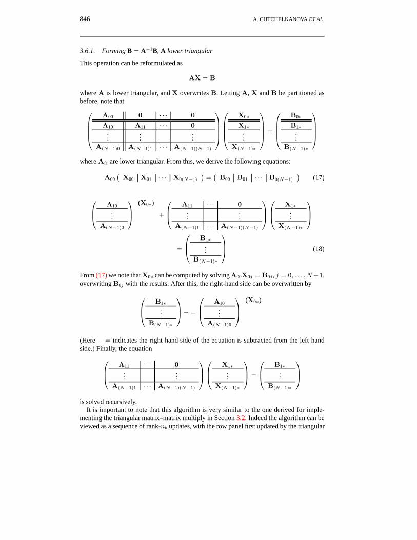
3.6.1. Forming B = A−1B, A lower triangular

This operation can be reformulated as

AX = B

where A is lower triangular, and X overwrites B. Letting A, X and B be partitioned asbefore, note that

A00 0 · · · 0

A10 A11 · · · 0...

......

A(N−1)0 A(N−1)1 · · · A(N−1)(N−1)

X0∗

X1∗...

X(N−1)∗

=

B0∗

B1∗...

B(N−1)∗

where Aii are lower triangular. From this, we derive the following equations:

A00(

X00 X01 · · · X0(N−1)

)=(

B00 B01 · · · B0(N−1)

)(17)

A10...

A(N−1)0

(X0∗)

+

A11 · · · 0...

...A(N−1)1 · · · A(N−1)(N−1)

X1∗

...X(N−1)∗

=

B1∗...

B(N−1)∗

(18)

From (17) we note that X0∗ can be computed by solving A00X0j = B0j , j = 0, . . . , N−1,overwriting B0j with the results. After this, the right-hand side can be overwritten by

B1∗...

B(N−1)∗

− =

A10...

A(N−1)0

(X0∗)

(Here − = indicates the right-hand side of the equation is subtracted from the left-handside.) Finally, the equation A11 · · · 0

......

A(N−1)1 · · · A(N−1)(N−1)

X1∗

...X(N−1)∗

=

B1∗...

B(N−1)∗

is solved recursively.

It is important to note that this algorithm is very similar to the one derived for imple-menting the triangular matrix–matrix multiply in Section 3.2. Indeed the algorithm can beviewed as a sequence of rank-nb updates, with the row panel first updated by the triangular


solve with multiple right-hand sides in equation (17). Also the order of the updates is thereverse of the corresponding updates for the lower triangular matrix multiply.

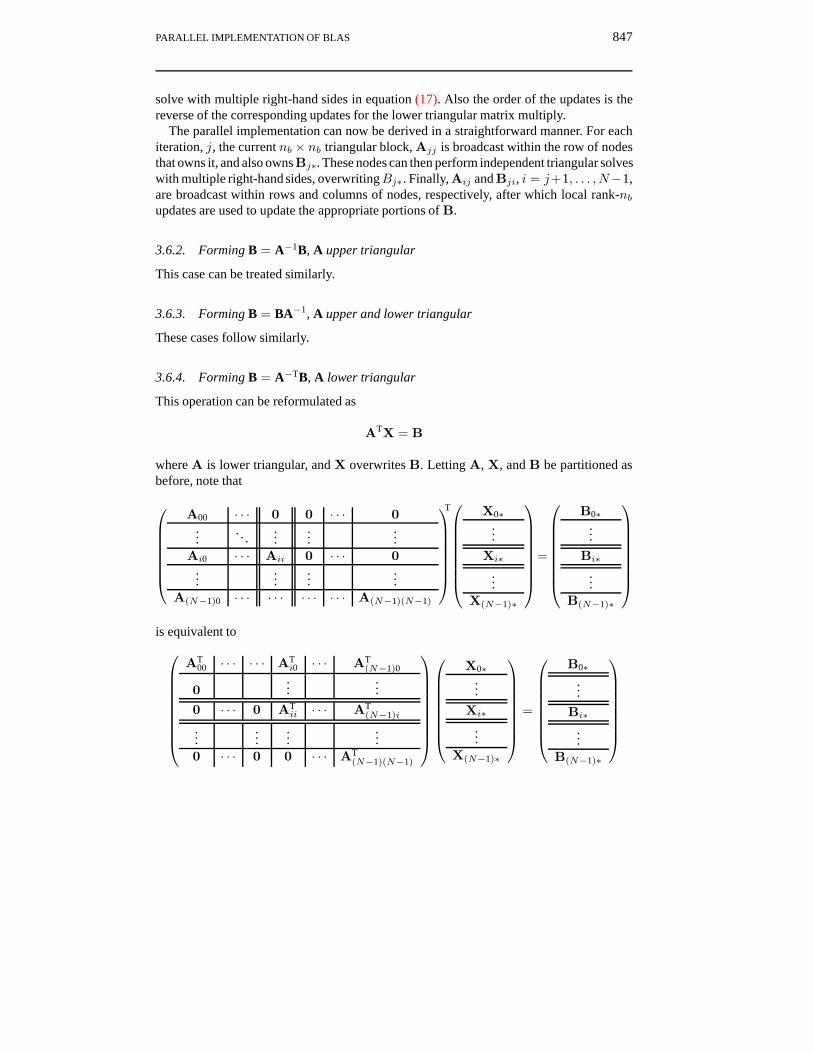
The parallel implementation can now be derived in a straightforward manner. For eachiteration, j, the current nb × nb triangular block, Ajj is broadcast within the row of nodesthat owns it, and also owns Bj∗. These nodes can then perform independent triangular solveswith multiple right-hand sides, overwritingBj∗. Finally, Aij and Bji, i = j+1, . . . , N−1,are broadcast within rows and columns of nodes, respectively, after which local rank-nbupdates are used to update the appropriate portions of B.

3.6.2. Forming B = A−1B, A upper triangular


3.6.3. Forming B = BA−1, A upper and lower triangular

These cases follow similarly.

3.6.4. Forming B = A−TB, A lower triangular

This operation can be reformulated as

ATX = B

where A is lower triangular, and X overwrites B. Letting A, X, and B be partitioned asbefore, note that

A00 · · · 0 0 · · · 0...

. . ....

......

Ai0 · · · Aii 0 · · · 0...

......

...A(N−1)0 · · · · · · · · · · · · A(N−1)(N−1)

T

X0∗...

Xi∗...

X(N−1)∗

=

B0∗...

Bi∗...

B(N−1)∗

is equivalent to

AT00 · · · · · · AT

i0 · · · AT(N−1)0

0...

...

0 · · · 0 ATii · · · AT

(N−1)i

......

......

0 · · · 0 0 · · · AT(N−1)(N−1)

X0∗...

Xi∗...

X(N−1)∗

=

B0∗...

Bi∗...

B(N−1)∗


From this, we derive the following equation:

ATiiXi∗ +

0...0

A(i+1)i

...A(N−1)i

T

X0∗...

Xi∗X(i+1)∗

...X(N−1)∗

= Bi∗

Taking advantage of zeros, the following two steps will compute Xi∗:

Bi∗ = Bi∗ −

A(i+1)i

...A(N−1)i

T X(i+1)∗

...X(N−1)∗

(19)

followed by solvingATiiXi∗ = Bi∗ (20)

Note that Xi∗ must be computed in the order i = N − 1, . . . , 0, which also allows B to beoverwritten by X as the computation proceeds.

Again, observe the similarity with the operation B = ATB, where A is lower triangular.Exploiting this similarity, we obtain the following parallel algorithm. At step i, non-zeroblocks Aji are broadcast within rows. After computing local contributions of the updatein equation (19), the results are summed within columns to the row of nodes that holdsthe ith panel of B. Finally, local triangular solves with multiple right-hand-sides to updateaccording to equation (20) are performed, and i is decreased.

3.6.5. Forming B = A−TB, A upper triangular


3.6.6. Forming B = BA−T, A upper and lower triangular

These cases follow similarly.

4. ANALYSIS

In [15], we gave an analysis of the matrix–matrix multiplication algorithm. In that paper,we assumed a slightly different matrix distribution, and hence the results were slightlydifferent from those we derive next. In addition, we show the results of similar analysis ofother representative parallel Level 3 BLAS.

For our analysis, we make the following assumptions:

1. The nodes for a physical r× c mesh, with P ij assigned to the (i, j) physical node inthat mesh, are given.


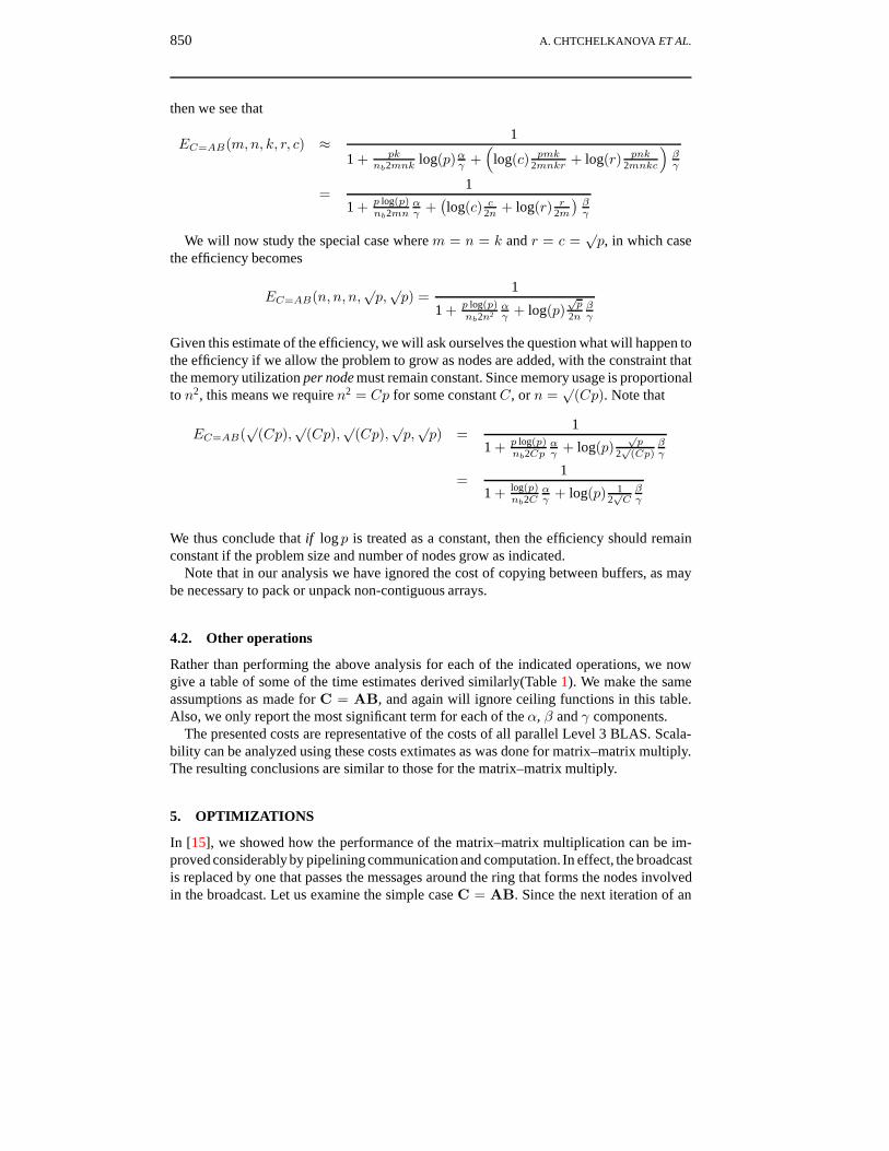
2. All alignment parameters equal one (i.e. the matrices are aligned to the upper-leftelement of the template matrix.)

3. nr = nc = nb.4. A minimum spanning tree broadcast and summation-to-one are used, so that the cost

for broadcasting a vector of length n among p nodes is given by

dlog(p)e(α + nβ)

and the cost for summing vectors of length n among p nodes is given by

dlog(p)e(α+ nβ + nγ)

There are a number of papers on how to improve upon this method of broadcastingand summation[20,23–25], but will analyze only this simple approach, since it istypically the current MPI default implementation.

5. Dimensions m, n and k are integer multiples of nb: m = Mnb, n = Nnb andk = Knb.

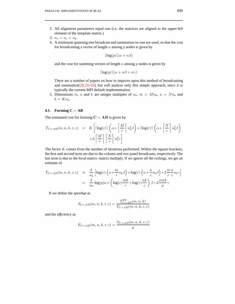
4.1. Forming C = AB

The estimated cost for forming C = AB is given by

TC=AB(m,n, k, r, c) = K

[dlog(c)e

(α+

⌈M

r

⌉n2bβ

)+dlog(r)e

(α+

⌈N

c

⌉n2bβ

)+2

⌈M

r

⌉⌈N

c

⌉n3bγ

]The factor K comes from the number of iterations performed. Within the square brackets,the first and second term are due to the column and row panel broadcasts, respectively. Thelast term is due to the local matrix–matrix multiply. If we ignore all the ceilings, we get anestimate of

TC=AB(m,n, k, r, c) ≈ k

nb

[log(c)

(α+

m

rnbβ

)+log(r)

(α+

n

cnbβ

)+2

m

r

n

cnbγ]

=k

nblog(p)α+

(log(c)

mk

r+log(r)

nk

c

)β+2

mnk

pγ

If we define the speedup as

SC=AB(m,n, k, r, c) =T

seqC=AB(m,n, k)

TC=AB(m,n, k, r, c)

and the efficiency as

EC=AB(m,n, k, r, c) =SC=AB(m,n, k, r, c)

p


then we see that

EC=AB(m,n, k, r, c) ≈ 1

1 + pknb2mnk log(p)αγ +

(log(c) pmk

2mnkr + log(r) pnk2mnkc

)βγ

=1

1 + p log(p)nb2mn

αγ +

(log(c) c

2n + log(r) r2m

)βγ

We will now study the special case where m = n = k and r = c =√p, in which case

the efficiency becomes

EC=AB(n, n, n,√p,√p) =

1

1 + p log(p)nb2n2

αγ + log(p)

√p

2nβγ

Given this estimate of the efficiency, we will ask ourselves the question what will happen tothe efficiency if we allow the problem to grow as nodes are added, with the constraint thatthe memory utilization per node must remain constant. Since memory usage is proportionalto n2, this means we require n2 = Cp for some constant C, or n =

√(Cp). Note that

EC=AB(√

(Cp),√

(Cp),√

(Cp),√p,√p) =

1

1 + p log(p)nb2Cp

αγ + log(p)

√p

2√

(Cp)βγ

=1

1 + log(p)nb2C

αγ + log(p) 1

2√Cβγ

We thus conclude that if log p is treated as a constant, then the efficiency should remainconstant if the problem size and number of nodes grow as indicated.

Note that in our analysis we have ignored the cost of copying between buffers, as maybe necessary to pack or unpack non-contiguous arrays.

4.2. Other operations

Rather than performing the above analysis for each of the indicated operations, we nowgive a table of some of the time estimates derived similarly(Table 1). We make the sameassumptions as made for C = AB, and again will ignore ceiling functions in this table.Also, we only report the most significant term for each of the α, β and γ components.

The presented costs are representative of the costs of all parallel Level 3 BLAS. Scala-bility can be analyzed using these costs extimates as was done for matrix–matrix multiply.The resulting conclusions are similar to those for the matrix–matrix multiply.

5. OPTIMIZATIONS

In [15], we showed how the performance of the matrix–matrix multiplication can be im-proved considerably by pipelining communication and computation. In effect, the broadcastis replaced by one that passes the messages around the ring that forms the nodes involvedin the broadcast. Let us examine the simple case C = AB. Since the next iteration of an


Table 1. Algorithm costs

Algorithm Cost

xGEMM (m× n matrix C, n× k matrix A)

TGEMMC=AB ≈ TC=ABT ≈ TC=ATB ≈ log(p) knbα+

(log(c)mk

r+ log(r)nk

c

)β + 2mnk

pγ

xTRMM (m× n matrix B)

TTRMMB=AB ≈ TTRMMB=ATB ≈ log(p) mnbα+

(log(c)m

2

2r + log(r)mnc

))β + m2n

pγ

xSYMM(m× n matrix C)

TSYMMC=AB ≈ TTRMMC=AB + TRTRMMC=ATB

xSYRK (m× n matrix A)

TSYRKC=AAT ≈nnb

log(p)α+(

log(c)mn2r + log(r)mnc

)β + mn2

pγ

TSYRKC=ATA ≈mnb

log(p)α+(

log(c)mn2r + log(r)mnc

)β + m2n

pγ

xSYR2K (m× n matrices A and B)

TSYR2KC=ABT+BTA ≈ TSYRKC=AAT + TSYRKC=ATA

xTRSM (m× n matrix B)

TTRSMB=A−1B ≈(

log(p) + log(c))mnbα+

(log(c)m

2

2r + log(r)mnc

)β

+nm2

pγ

algorithm can start as soon as the next nodes that need to broadcast are ready, the net costof the algorithm becomes

TC=AB(m,n, k, r, c)

= K

[2

(α+

⌈M

r

⌉n2bβ

)+ 2

(α+

⌈N

c

⌉n2bβ

)+ 2

⌈M

r

⌉⌈N

c

⌉n3bγ

]≈ k

nb2α+

(2mk

r+ 2

nk

c

)β + 2

mnk

pγ

This formula ignores the cost of filling and/or emptying the pipe. A similar improvement isseen for all the algorithms if this ‘ring’ broadcast is used. For some of the algorithms, somecare must be taken to make the operation ‘flow’ in the appropriate direction. Note that theeffect on scalability is considerable, since in the estimate for the efficiency, the ‘log’ factorsare essentially replaced by a 2, making the approach virtually perfectly scalable.

6. PERFORMANCE RESULTS

This Section reports the performance of preliminary parallel Level 3 BLAS implemen-tations, obtained on an Intel Paragon with GP nodes (one compute processor per node).Our implementations use the highly optimized BLAS library available for computation oneach node. Communication is accomplished using MPI collective communication calls.We present results from pipelined implementations.

In Figure 4, we show the performance of representative parallel Level 3 BLAS as a


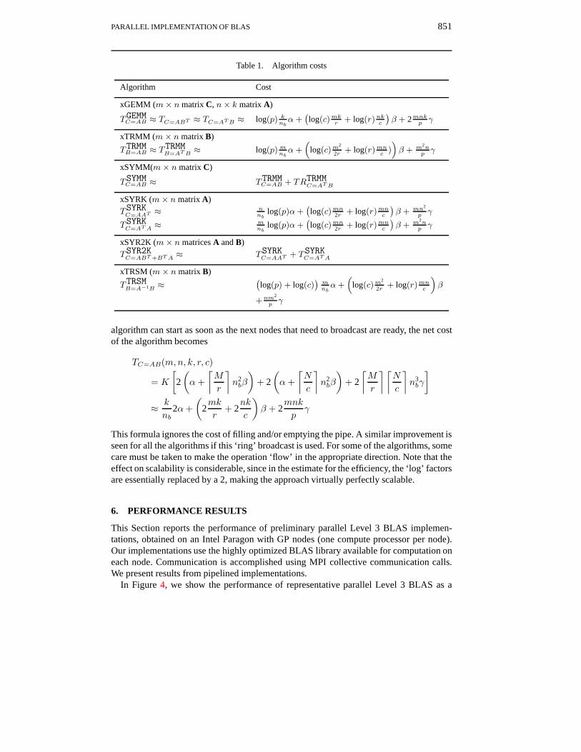
Figure 4. Performance of the various algorithms (on a single node), as a function of the globalmatrix dimension. The ‘ x x x x’ denoted the different options passed to the BLAS routine, e.g.

r u t n stands for ‘Right’, ‘Upper triangular’, ‘Transpose’, ‘No transpose’

function of the matrix dimensions, on a single node. This gives us an indication of the peakperformance for the different operations.

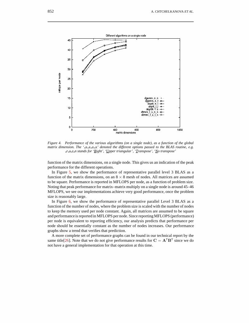
In Figure 5, we show the performance of representative parallel level 3 BLAS as afunction of the matrix dimensions, on an 8 × 8 mesh of nodes. All matrices are assumedto be square. Performance is reported in MFLOPS per node, as a function of problem size.Noting that peak performance for matrix–matrix multiply on a single node is around 45–46MFLOPS, we see our implementations achieve very good performance, once the problemsize is reasonably large.

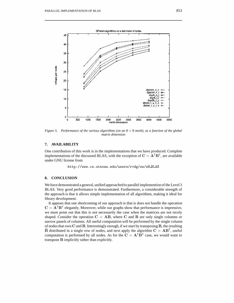
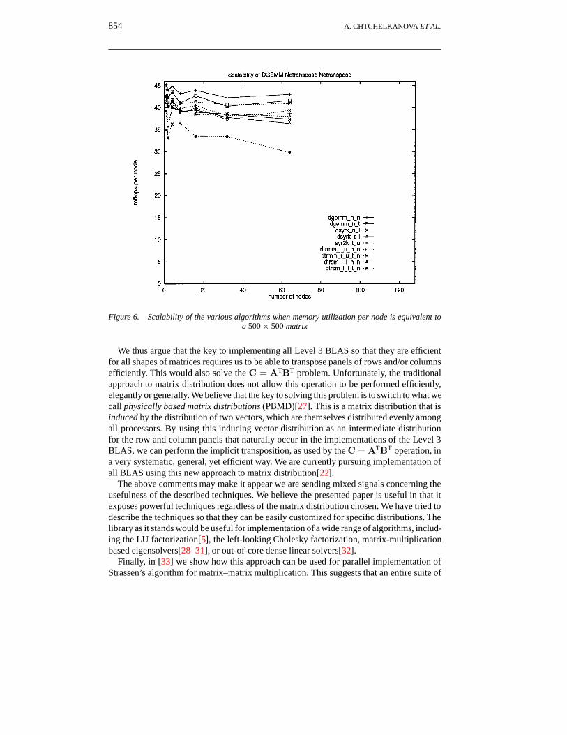
In Figure 6, we show the performance of representative parallel Level 3 BLAS as afunction of the number of nodes, where the problem size is scaled with the number of nodesto keep the memory used per node constant. Again, all matrices are assumed to be squareand performance is reported in MFLOPS per node. Since reporting MFLOPS (performance)per node is equivalent to reporting efficiency, our analysis predicts that performance pernode should be essentially constant as the number of nodes increases. Our performancegraphs show a trend that verifies that prediction.

A more complete set of performance graphs can be found in our technical report by thesame title[26]. Note that we do not give performance results for C = ATBT since we donot have a general implementation for that operation at this time.


Figure 5. Performance of the various algorithms (on an 8 × 8 mesh), as a function of the globalmatrix dimension

7. AVAILABILITY

One contribution of this work is in the implementations that we have produced. Completeimplementations of the discussed BLAS, with the exception of C = ATBT, are availableunder GNU license from

http://www.cs.utexas.edu/users/rvdg/sw/sB BLAS

8. CONCLUSION

We have demonstrated a general, unified approached to parallel implemention of the Level 3BLAS. Very good performance is demonstrated. Furthermore, a considerable strength ofthe approach is that it allows simple implementation of all algorithms, making it ideal forlibrary development.

It appears that one shortcoming of our approach is that is does not handle the operationC = ATBT elegantly. Moreover, while our graphs show that performance is impressive,we must point out that this is not necessarily the case when the matrices are not nicelyshaped. Consider the operation C = AB, where C and B are only single columns ornarrow panels of columns. All useful computation will be performed by the single columnof nodes that own C and B. Interestingly enough, if we start by transposing B, the resultingB distributed in a single row of nodes, and next apply the algorithm C = ABT, usefulcomputation is performed by all nodes. As for the C = ATBT case, we would want totranspose B implicitly rather than explicitly.


Figure 6. Scalability of the various algorithms when memory utilization per node is equivalent toa 500× 500 matrix

We thus argue that the key to implementing all Level 3 BLAS so that they are efficientfor all shapes of matrices requires us to be able to transpose panels of rows and/or columnsefficiently. This would also solve the C = ATBT problem. Unfortunately, the traditionalapproach to matrix distribution does not allow this operation to be performed efficiently,elegantly or generally. We believe that the key to solving this problem is to switch to what wecall physically based matrix distributions (PBMD)[27]. This is a matrix distribution that isinduced by the distribution of two vectors, which are themselves distributed evenly amongall processors. By using this inducing vector distribution as an intermediate distributionfor the row and column panels that naturally occur in the implementations of the Level 3BLAS, we can perform the implicit transposition, as used by the C = ATBT operation, ina very systematic, general, yet efficient way. We are currently pursuing implementation ofall BLAS using this new approach to matrix distribution[22].

The above comments may make it appear we are sending mixed signals concerning theusefulness of the described techniques. We believe the presented paper is useful in that itexposes powerful techniques regardless of the matrix distribution chosen. We have tried todescribe the techniques so that they can be easily customized for specific distributions. Thelibrary as it stands would be useful for implementation of a wide range of algorithms, includ-ing the LU factorization[5], the left-looking Cholesky factorization, matrix-multiplicationbased eigensolvers[28–31], or out-of-core dense linear solvers[32].

Finally, in [33] we show how this approach can be used for parallel implementation ofStrassen’s algorithm for matrix–matrix multiplication. This suggests that an entire suite of


variants of Strassen’s algorithm for all the Level 3 BLAS could be implemented on top ofour standard parallel Level 3 BLAS implementations.

ACKNOWLEDGEMENTS

This research was performed in part using the Intel Paragon System operated by theCalifornia Institute of Technology on behalf of the Concurrent Supercomputing Consor-tium. Access to this facility was provided by Intel Supercomputer Systems Division and theCalifornia Institute of Technology. This work is partially supported by the NASA High Per-formance Computing and Communications Program’s Earth and Space Sciences Projectunder NRA Grant NAG5-2497 and the PRISM project, which is sponsored by ARPA.Additional support came from the Intel Research Council.

REFERENCES

1. E. Anderson, A. Benzoni, J. Dongarra, S. Moulton, S. Ostrouchov, B. Tourancheau and R. van deGeijn, ‘LAPACK for distributed memory architectures: progress report’, in Proceedings of theFifth SIAM Conference on Parallel Processing for Scientific Computing, SIAM, Philadelphia,1992, pp. 625–630.

2. J. Choi, J. J. Dongarra, R. Pozo and D. W. Walker, ‘Scalapack: A scalable linear algebra libraryfor distributed memory concurrent computers’, Proceedings of the Fourth Symposium on theFrontiers of Massively Parallel Computation, IEEE Comput. Soc. Press, 1992, pp. 120-127.

3. J. Demmel, J. Dongarra, R. van de Geijn and D. Walker, ‘LAPACK for distributed memoryarchitectures: The next generation’, in Proceedings of the Sixth SIAM Conference on ParallelProcessing for Scientific Computing, Norfolk, March 1993.

4. J. Dongarra and R. van de Geijn, ‘A parallel dense linear solve library routine’, in Proceedingsof the 1992 Intel Supercomputer Users’ Group Meeting, Dallas, Oct. 1992.

5. J. Dongarra, R. van de Geijn and D.Walker, ‘Scalability issues affecting the design of a denselinear algebra library’, Special Issue on Scalability of Parallel Algorithms, J. Parallel Distrib.Comput., 22, (3), (1994).

6. G. C. Fox, M. A. Johnson, G. A. Lyzenga, S. W. Otto, J. K. Salmon and D. W. Walker, SolvingProblems on Concurrent Processors, Vol. 1, Prentice Hall, Englewood Cliffs, N.J., 1988.

7. W. Lichtenstein and S. L. Johnsson, ‘Block-cyclic dense linear algebra’, Harvard University,Center for Research in Computing Technology, TR-04-92, Jan. 1992.

8. R. van de Geijn, ‘Massively parallel LINPACK benchmark on the Intel Touchstone DELTA andiPSC/860 systems: Preliminary report’, TR-91-28, Department of Computer Sciences, Universityof Texas, Aug. 1991.

9. E. Anderson, Z. Bai, C. Bischof, J. Demmel, J. Dongarra, J. DuCroz, A. Greenbaum, S. Ham-marling, A. McKenney and D. Sorensen, ‘Lapack: A portable linear algebra library for highperformance computers’, Proceedings of Supercomputing ’90, IEEE Press, 1990, pp. 1–10.

10. E. Anderson, Z. Bai, J. Demmel, J. Dongarra, J. DuCroz, A. Greenbaum, S. Hammarling,A. McKenney, S. Ostrouchov and D. Sorensen, LAPACK Users’ Guide, SIAM, Philadelphia,1992.

11. C. L. Lawson, R. J. Hanson, D. R. Kincaid and F. T. Krogh, ‘Basic linear algebra subprogramsfor Fortran usage’, TOMS, 5, (3), 308–323 (1979).

12. J. J. Dongarra, J. Du Croz, S. Hammarling and R. J. Hanson, ‘An extended set of FORTRANbasic linear algebra subprograms’, TOMS, 14, (1), 1–17 (1988).

13. J. J. Dongarra, J. Du Croz, S. Hammarling and I. Duff, ‘A set of Level 3 basic linear algebrasubprograms’, TOMS, 16, (1), 1–16 (1990).

14. J. Choi, J. Dongarra, S. Ostrouchov, A. Petitet, D. Walker, and R. C. Whaley ‘A proposal fora set of parallel basic linear algebra subprograms’, LAPACK Working Note 100, University ofTennessee, CS-95-292, May 1995.


15. R. van de Geijn and J. Watts, ‘SUMMA: Scalable universal matrix multiplication algorithm’,TR-95-13, Department of Computer Sciences, University of Texas, April 1995. Also: LAPACKWorking Note 96, May 1, Concurrency: Pract. Exp., 9, (4), 255–274 (1997).

16. J. Choi, J. J. Dongarra and D. W. Walker, ‘PUMMA: Parallel universal matrix multiplicationalgorithms on distributed memory concurrent computers’, Concurrency: Pract. Exp., 6, (7),543–570 (1994).

17. S. Huss-Lederman, E. Jacobson and A. Tsao, ‘Comparison of scalable parallel matrix multipli-cation libraries’, in Proceedings of the Scalable Parallel Libraries Conference, Starksville, MS,Oct. 1993.

18. S. Huss-Lederman, E. Jacobson, A. Tsao and G. Zhang, ‘Matrix multiplication on the IntelTouchstone DELTA’, Concurrency: Pract. Exp., 6, (7), 571-594 (1994).

19. B. Kagstrom and C. F. Van Loan, Gemm-based level-3 blas, 1991. Theory Center TechnicalReport, January 1991.

20. P. Mitra, D. Payne, L. Shuler, R. van de Geijn and J. Watts, ‘Fast collective communicationlibraries, please’, in the Proceedings of the Intel Supercomputing Users’ Group Meeting 1995.

21. R. C. Agarwal, F. G. Gustavson, S. M. Balle, M. Joshi and P. Palkar, ‘A high performance matrixmultiplication algorithm for MPPs’, IBM T.J. Watson Research Center, 1995.

22. A. Chtchelkanova, C. Edwards, J. Gunnels, G. Morrow, J. Overfelt and R A. van de Geijn,‘Towards usable and lean parallel linear algebra libraries’, TR-96-09, Department of ComputerSciences, University of Texas, May 1996.

23. C.-T. Ho and S. L. Johnsson, ‘Distributed routing algorithms for broadcasting and personalizedcommunication in hypercubes’, in Proceedings of the 1986 International Conference on ParallelProcessing, IEEE, 1986, pp. 640–648.

24. R. van de Geijn, ‘On global combine operations’, J Parallel Distrib. Comput., 22, 324-328(1994).

25. J. Watts and R. van de Geijn, ‘A pipelined broadcast for multidimensional meshes’, ParallelProcess. Lett., 5, (2), 281–292 (1995).

26. A. Chtchelkanova, J. Gunnels, G. Morrow, J. Overfelt and R. A. van de Geijn, ‘Parallel imple-mentation of BLAS: General techniques for Level 3 BLAS’, TR-95-40, Department of ComputerSciences, University of Texas, Oct. 1995.

27. C. Edwards, P. Geng, A. Patra, and R. van de Geijn, ‘Parallel matrix distributions: have we beendoing it all wrong?’, Department of Computer Sciences, UT-Austin, Report TR95-39, Oct. 1995.

28. L. Auslander and A.Tsao, ‘On parallelizable eigensolvers’, Adv. Appl. Math., 13, 253–261,(1992).

29. Z. Bai and J. Demmel, ‘Design of a parallel nonsymmetric eigenroutine toolbox, Part I’, ParallelProcessing for Scientific Computing, R. Sincovec, D. Keyes, M. Leuze, L. Petzold and D. Reed(Eds.), SIAM Publications, Philadelphia, PA, 1993, pp. 391–398.

30. Z. Bai, J. Demmel, J. Dongarra, A. Petitet, H. Robinson and K. Stanley, The Spectral Decomposi-tion of Nonsymmetric Matrices on Distributed Memory Parallel Computers, LAPACK workingnote 91, University of Tennessee, Jan. 1995.

31. S. Lederman, A. Tsao and T. Turnbull, ‘A parallelizable eigensolver for real diagonalizablematrices with real eigenvalues’, Technical Report TR-91-042, Supercomputing Research Center,1991.

32. K. Klimkowski and R. van de Geijn, ‘Anatomy of an out-of-core dense linear solver’, Vol III,Algorithms and Applications, Proceedings of the 1995 International Conference on ParallelProcessing, pp. 29–33.

33. B. Grayson and R. van de Geijn, ‘A high performance parallel strassen implementation’, ParallelProcess. Lett., to be published.

34. R. C. Agarwal, F. G. Gustavson and M. Zubair, ‘A high performance matrix multiplicationalgorithm on a distributed-memory parallel computer, using overlapped communication’, IBMJ. Res. Dev., 673–681 (1994).

35. L. E. Cannon, A Cellular Computer to Implement the Kalman Filter Algorithm, Ph.D. thesis,1969, Montana State University.

36. J. Choi, J. J. Dongarra and D. W. Walker, ‘Level 3 BLAS for distributed memory concurrentcomputers’, CNRS-NSF Workshop on Environments and Tools for Parallel Scientific Computing,Saint Hilaire du Touvet, France, 7-8 Sept. 1992, Elsevier Science Publishers, 1992.


37. J. J. Dongarra, I. S. Duff, D. C. Sorensen and H. A. van der Vorst, Solving Linear Systems onVector and Shared Memory Computers, SIAM, Philadelphia, 1991.

38. J. J. Dongarra, R. A. van de Geijn and R. Clint Whaley, ‘Two dimensional basic linear alge-bra communication subprograms’, in Proceedings of the Sixth SIAM Conference on ParallelProcessing for Scientific Computing, Norfolk, March 1993.

39. G. Fox, S. Otto and A. Hey, ‘Matrix algorithms on a hypercube I: Matrix multiplication’, ParallelComput., 3, 17-31 (1987).

40. G. H. Golub and C. F. Van Loan, Matrix Computations, Johns Hopkins University Press, 2ndedn., 1989.

41. W. Gropp, E. Lusk and A. Skjellum, Using MPI: Portable Programming with the Message-Passing Interface, The MIT Press, 1994.

42. B. Kagstrom and P. Ling, ‘Level 2 and 3 BLAS routines for the IBM 3090 VF/400: Implemen-tation and experiences’, Technical Report UMINF-154.88, Information Processing, Universityof Umea, S-901 87 Umea, Sweden, 1988.

43. J. G. Lewis and R. A. van de Geijn, ‘Implementing matrix-vector multiplication and conjugategradient algorithms on distributed memory multicomputers’, Supercomputing ’93.

44. J. G. Lewis, D. G. Payne and R. A. van de Geijn, ‘Matrix-vector multiplication and conjugategradient algorithms on distributed memory computers’, Scalable High Performance ComputingConference, 1994.

45. C. Lin and L. Snyder, ‘A matrix product algorithm and its comparative performance on hyper-cubes’, in Proceedings of Scalable High Performance Computing Conference, Q. Stout and M.Wolfe (eds.), IEEE Press, Los Alamitos, CA, 1992, pp. 190–193.

Documents

Parallel implementation of BLAS: general techniques for Level 3 BLAS